Managing Managing DistributedDistributed Data Data Streams – IIStreams – II

Slides based on the Cormode/GarofalakisSlides based on the Cormode/GarofalakisVLDB’2006 tutorialVLDB’2006 tutorial

2

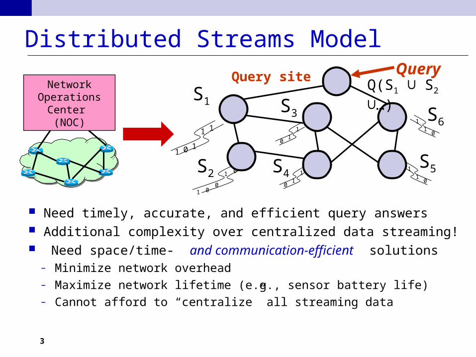
Distributed Streams Model

Large-scale querying/monitoring: Inherently distributed!– Streams physically distributed across remote sites

E.g., stream of UDP packets through subset of edge routers Challenge is “holistic” querying/monitoring

– Queries over the union of distributed streams Q(S1 ∪ S2 ∪ …)

– Streaming data is spread throughout the network

Network Operations

Center (NOC)

Query site Query

0 11

1 1

00

1

1 0

0

11

0

11

0

11

0

11

Q(S1 ∪ S2 ∪…)

S6

S5S4

S3

S1

S2

3

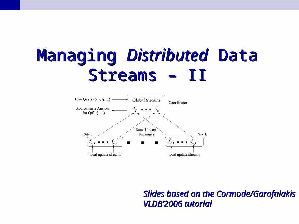
Distributed Streams Model

Need timely, accurate, and efficient query answers Additional complexity over centralized data streaming! Need space/time- and communication-efficient solutions

– Minimize network overhead– Maximize network lifetime (e.g., sensor battery life)– Cannot afford to “centralize” all streaming data

Network Operations

Center (NOC)

Query site Query

0 11

1 1

00

1

1 0

0

11

0

11

0

11

0

11

Q(S1 ∪ S2 ∪…)

S6

S5S4

S3

S1

S2

4

Outline

Introduction, Motivation, Problem Setup One-Shot Distributed-Stream Querying

– Tree Based Aggregation

– Robustness and Loss

– Decentralized Computation and Gossiping

Continuous Distributed-Stream Tracking Probabilistic Distributed Data Acquisition Conclusions

Robustness and Loss

6

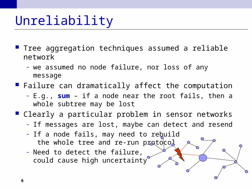
Unreliability

Tree aggregation techniques assumed a reliable network– we assumed no node failure, nor loss of any message

Failure can dramatically affect the computation– E.g., sum – if a node near the root fails, then a whole

subtree may be lost Clearly a particular problem in sensor networks

– If messages are lost, maybe can detect and resend– If a node fails, may need to rebuild

the whole tree and re-run protocol– Need to detect the failure,

could cause high uncertainty

7

Sensor Network Issues

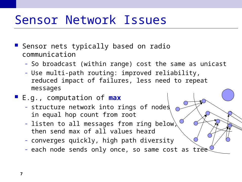
Sensor nets typically based on radio communication– So broadcast (within range) cost the same as unicast– Use multi-path routing: improved reliability, reduced impact

of failures, less need to repeat messages E.g., computation of max

– structure network into rings of nodes in equal hop count from root

– listen to all messages from ring below, then send max of all values heard

– converges quickly, high path diversity– each node sends only once, so same cost as tree

8

Order and Duplicate Insensitivity

It works because max is Order and Duplicate Insensitive (ODI) [Nath et al.’04]

Make use of the same e(), f(), g() framework as before Can prove correct if e(), f(), g() satisfy properties:

– g gives same output for duplicates: i=j ⇒ g(i) = g(j)– f is associative and commutative:

f(x,y) = f(y,x); f(x,f(y,z)) = f(f(x,y),z)– f is same-synopsis idempotent: f(x,x) = x

Easy to check min, max satisfy these requirements, sum does not

9

Applying ODI idea

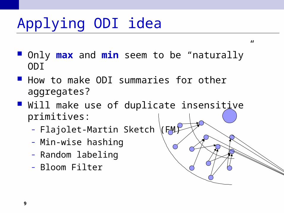
Only max and min seem to be “naturally” ODI How to make ODI summaries for other aggregates? Will make use of duplicate insensitive primitives:

– Flajolet-Martin Sketch (FM)– Min-wise hashing– Random labeling– Bloom Filter

12

FM Sketch – ODI Properties

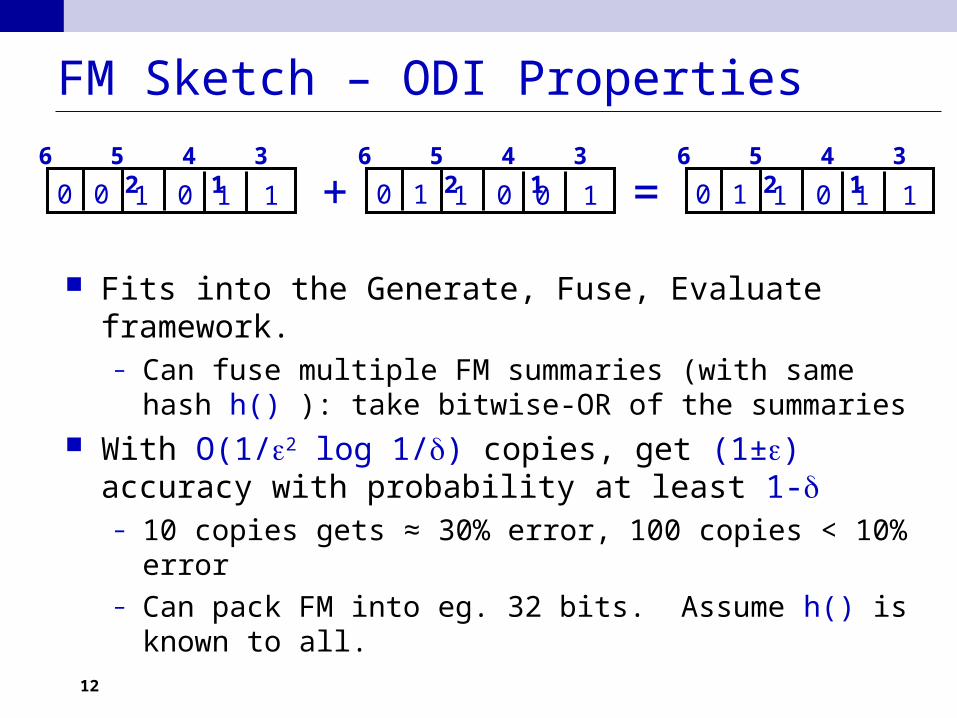
Fits into the Generate, Fuse, Evaluate framework.– Can fuse multiple FM summaries (with same hash h() ):

take bitwise-OR of the summaries With O(1/2 log 1/) copies, get (1±) accuracy with

probability at least 1-– 10 copies gets ≈ 30% error, 100 copies < 10% error– Can pack FM into eg. 32 bits. Assume h() is known to all.

00 0 1 11

6 5 4 3 2 1

00 1 1 10

6 5 4 3 2 1

00 1 1 11

6 5 4 3 2 1

+ =

13

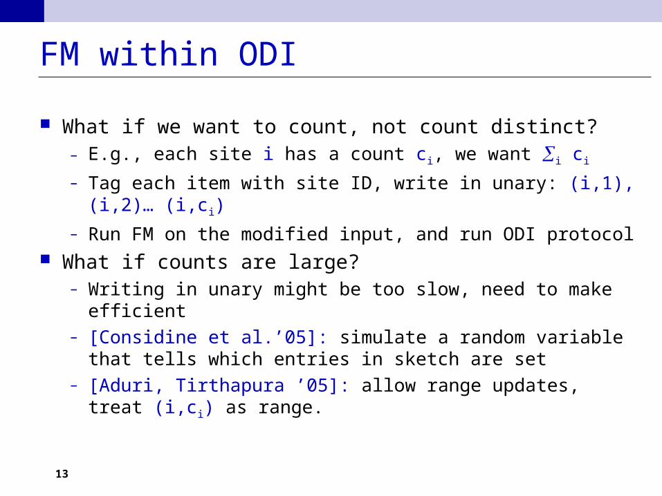
FM within ODI

What if we want to count, not count distinct? – E.g., each site i has a count ci, we want i ci

– Tag each item with site ID, write in unary: (i,1), (i,2)… (i,ci)

– Run FM on the modified input, and run ODI protocol What if counts are large?

– Writing in unary might be too slow, need to make efficient– [Considine et al.’05]: simulate a random variable that tells which

entries in sketch are set

– [Aduri, Tirthapura ’05]: allow range updates, treat (i,ci) as range.

14

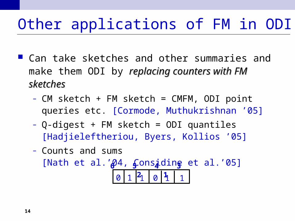
Other applications of FM in ODI

Can take sketches and other summaries and make them ODI by replacing counters with FM sketchesreplacing counters with FM sketches– CM sketch + FM sketch = CMFM, ODI point queries etc.

[Cormode, Muthukrishnan ’05]– Q-digest + FM sketch = ODI quantiles

[Hadjieleftheriou, Byers, Kollios ’05]– Counts and sums

[Nath et al.’04, Considine et al.’05]

00 1 1 11

6 5 4 3 2 1

15

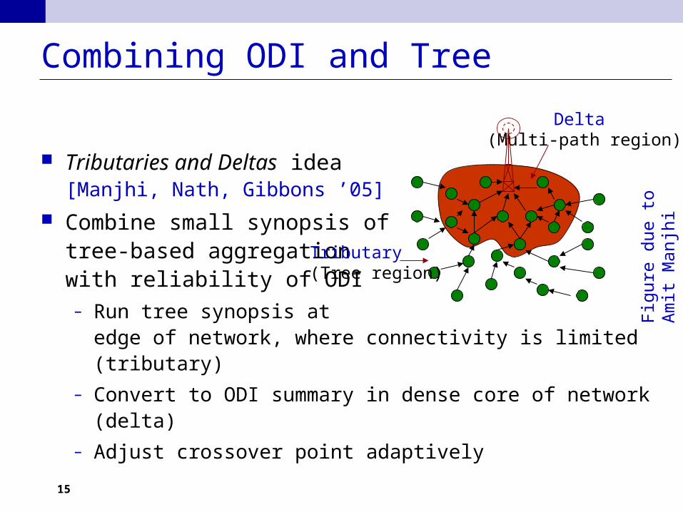
Combining ODI and Tree

Tributaries and Deltas idea[Manjhi, Nath, Gibbons ’05]

Combine small synopsis of tree-based aggregation with reliability of ODI– Run tree synopsis at

edge of network, where connectivity is limited (tributary)

– Convert to ODI summary in dense core of network (delta)

– Adjust crossover point adaptively

Delta (Multi-path region)

Tributary (Tree region)

Figu

re d

ue to

Am

it M

anjh

i

16

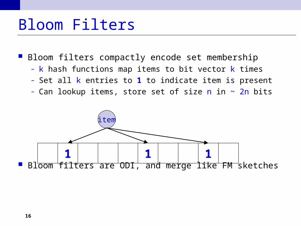
Bloom Filters

Bloom filters compactly encode set membership– k hash functions map items to bit vector k times– Set all k entries to 1 to indicate item is present– Can lookup items, store set of size n in ~ 2n bits

Bloom filters are ODI, and merge like FM sketches

item

1 1 1

17

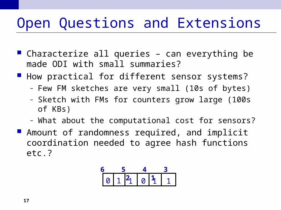
Open Questions and Extensions

Characterize all queries – can everything be made ODI with small summaries?

How practical for different sensor systems?– Few FM sketches are very small (10s of bytes)– Sketch with FMs for counters grow large (100s of KBs)– What about the computational cost for sensors?

Amount of randomness required, and implicit coordination needed to agree hash functions etc.?

00 1 1 11

6 5 4 3 2 1

18

Tutorial Outline Introduction, Motivation, Problem Setup One-Shot Distributed-Stream Querying Continuous Distributed-Stream Tracking

– Adaptive Slack Allocation

– Predictive Local-Stream Models

– Distributed Triggers

Probabilistic Distributed Data Acquisition Conclusions

19

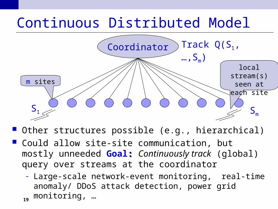
Continuous Distributed Model

Other structures possible (e.g., hierarchical) Could allow site-site communication, but mostly unneeded

Goal:: Continuously track (global) query over streams at the coordinator– Large-scale network-event monitoring, real-time anomaly/

DDoS attack detection, power grid monitoring, …

Coordinator

m sites

local stream(s) seen at each

site

S1 Sm

Track Q(S1,…,Sm)

20

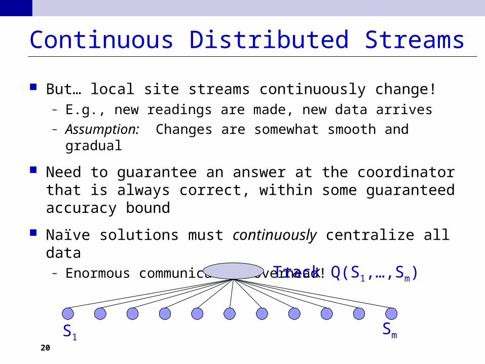
Continuous Distributed Streams

But… local site streams continuously change!– E.g., new readings are made, new data arrives– Assumption: Changes are somewhat smooth and gradual

Need to guarantee an answer at the coordinator that is always correct, within some guaranteed accuracy bound

Naïve solutions must continuously centralize all data – Enormous communication overhead!

S1Sm

Track Q(S1,…,Sm)

21

Challenges

Monitoring is Continuous…– Real-time tracking, rather than one-shot query/response

…Distributed…– Each remote site only observes part of the global stream(s)– Communication constraints: must minimize monitoring burden

…Streaming…– Each site sees a high-speed local data stream and can be

resource (CPU/memory) constrained …Holistic…

– Challenge is to monitor the complete global data distribution– Simple aggregates (e.g., aggregate traffic) are easier

22

How about Periodic Polling?

Sometimes periodic polling suffices for simple tasks– E.g., SNMP polls total traffic at coarse granularity

Still need to deal with holistic nature of aggregates Must balance polling frequency against communication

– Very frequent polling causes high communication, excess battery use in sensor networks

– Infrequent polling means delays in observing events

Need techniques to reduce communication while guaranteeing rapid response to events

23

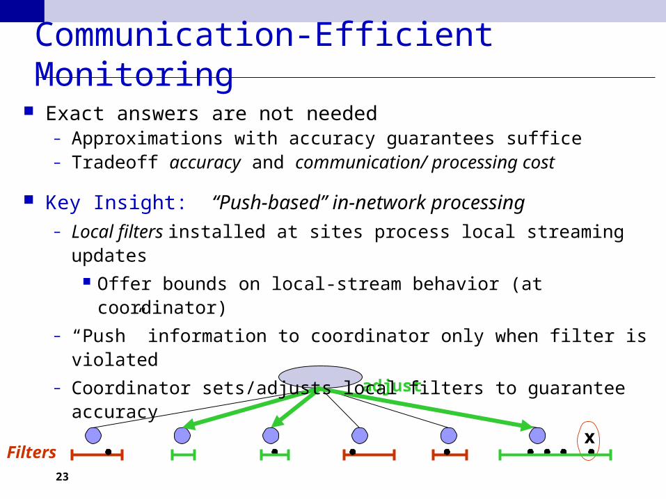
Communication-Efficient Monitoring

Filtersx

“push”

Filtersx

adjust

Exact answers are not needed– Approximations with accuracy guarantees suffice– Tradeoff accuracy and communication/ processing cost

Key Insight: “Push-based” in-network processing– Local filters installed at sites process local streaming updates

Offer bounds on local-stream behavior (at coordinator)

– “Push” information to coordinator only when filter is violated

– Coordinator sets/adjusts local filters to guarantee accuracy

Adaptive Slack Allocation

25

Slack Allocation

A key idea is Slack Allocation

Because we allow approximation, there is slack: the

tolerance for error between computed answer and truth

– May be absolute: |Y - Ŷ | slack is

– Or relative: Ŷ /Y (1±): slack is Y

For a given aggregate, show that the slack can be

divided between sites

Will see different slack division heuristics

26

Top-k Monitoring

Influential work on monitoring [Babcock, Olston’03]– Introduces some basic heuristics for dividing slack– Use local offset parameters so that all local distributions

look like the global distribution– Attempt to fix local slack violations by negotiation with

coordinator before a global readjustment– Showed that message delay does not affect correctness

Top 100

Imag

es fr

om h

ttp://

www.

billb

oard

.com

27

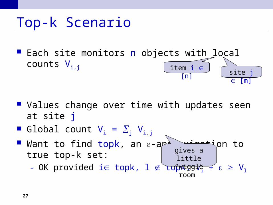
Top-k Scenario

Each site monitors n objects with local counts Vi,j

Values change over time with updates seen at site j Global count Vi = j Vi,j

Want to find topk, an -approximation to true top-k set:– OK provided i topk, l topk, Vi + Vl

item i [n]site j [m]

gives a little “wiggle room”

28

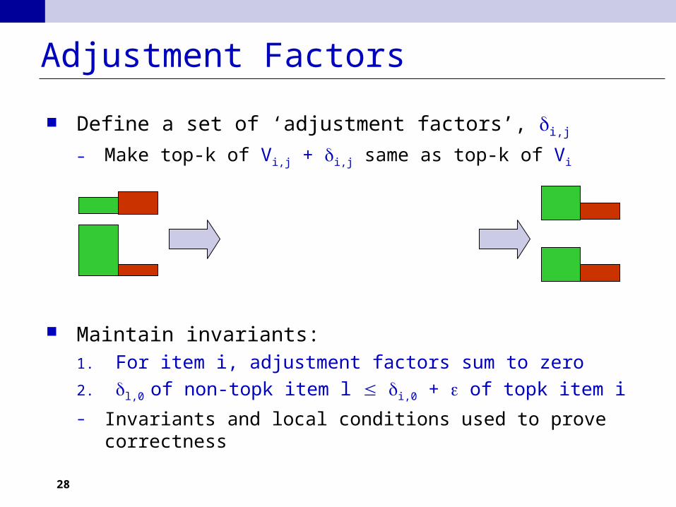
Adjustment Factors

Define a set of ‘adjustment factors’, i,j

– Make top-k of Vi,j + i,j same as top-k of Vi

Maintain invariants: 1. For item i, adjustment factors sum to zero

2. l,0 of non-topk item l i,0 + of topk item i

– Invariants and local conditions used to prove correctness

29

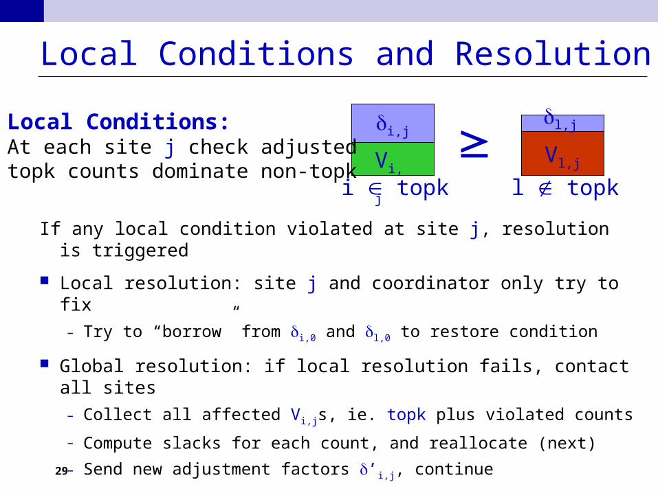
Local Conditions and Resolution

If any local condition violated at site j, resolution is triggered

Local resolution: site j and coordinator only try to fix

– Try to “borrow” from i,0 and l,0 to restore condition

Global resolution: if local resolution fails, contact all sites

– Collect all affected Vi,js, ie. topk plus violated counts

– Compute slacks for each count, and reallocate (next)

– Send new adjustment factors ’i,j, continue

i,j

Vi,j

i topk

Vl,j

l,j

l topk

Local Conditions:At each site j check adjusted topk counts dominate non-topk

30

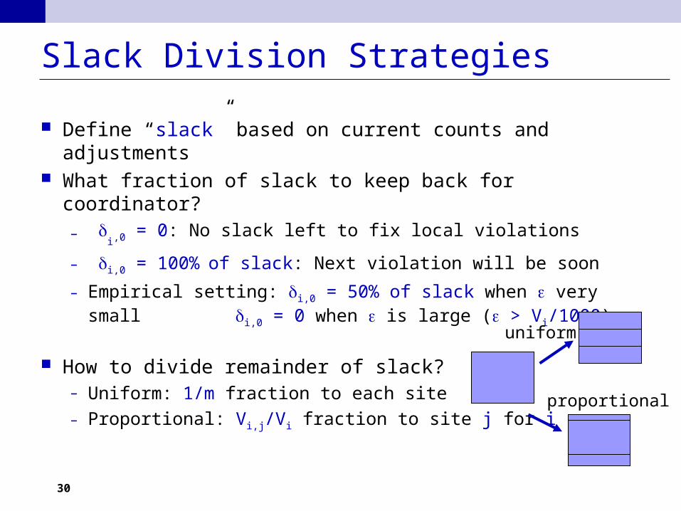
Slack Division Strategies

Define “slack” based on current counts and adjustments What fraction of slack to keep back for coordinator?

– i,0

= 0: No slack left to fix local violations

– i,0 = 100%of slack: Next violation will be soon

– Empirical setting: i,0 = 50% of slack when very small i,0 = 0 when is large ( > Vi/1000)

How to divide remainder of slack?– Uniform: 1/m fraction to each site

– Proportional: Vi,j/Vi fraction to site j for i

uniform

proportional

31

Pros and Cons

Result has many advantages:– Guaranteed correctness within approximation bounds

– Can show convergence to correct results even with delays

– Communication reduced by 1 order magnitude (compared to sending Vi,j whenever it changes by /m)

Disadvantages:– Reallocation gets complex: must check O(km) conditions

– Need O(n) space at each site, O(mn) at coordinator

– Large (≈ O(k)) messages

– Global resyncs are expensive: m messages to k sites

32

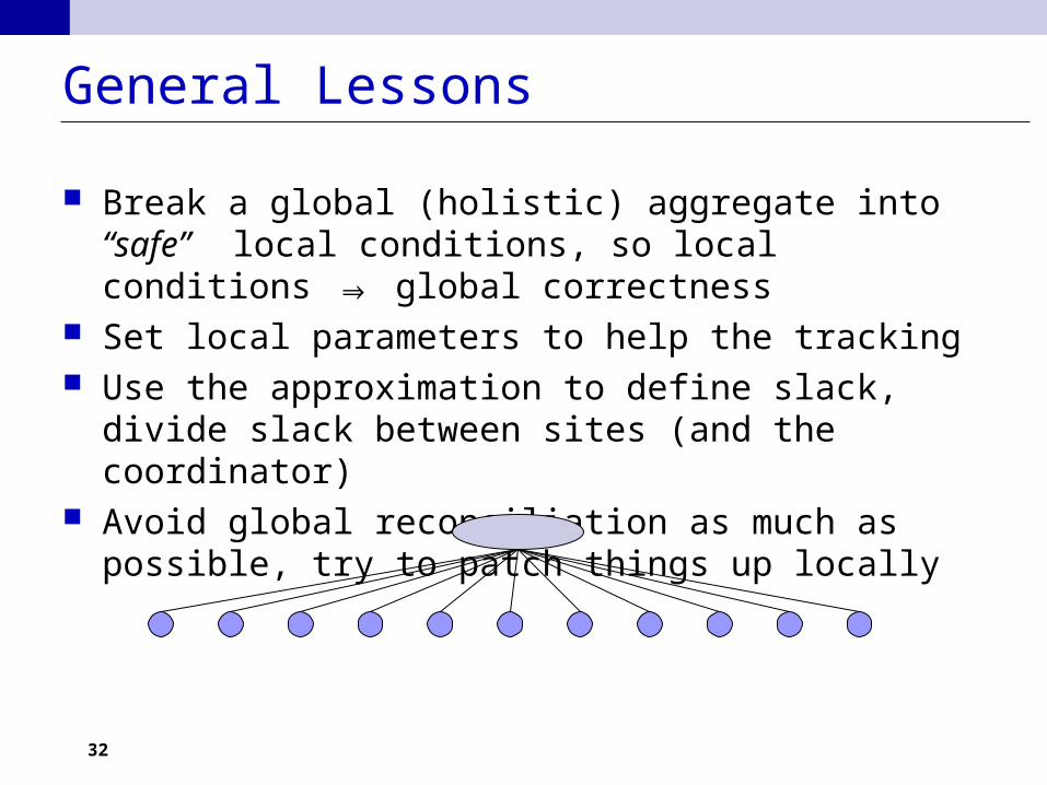
General Lessons

Break a global (holistic) aggregate into “safe” local conditions, so local conditions ⇒ global correctness

Set local parameters to help the tracking Use the approximation to define slack, divide slack

between sites (and the coordinator) Avoid global reconciliation as much as possible, try to

patch things up locally

Predictive Local-Stream Models

34

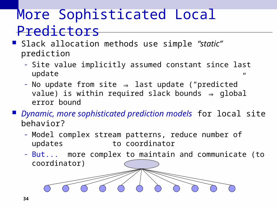
More Sophisticated Local Predictors Slack allocation methods use simple “static” prediction

– Site value implicitly assumed constant since last update – No update from site ⇒ last update (“predicted” value) is within

required slack bounds ⇒ global error bound Dynamic, more sophisticated prediction models for local

site behavior?– Model complex stream patterns, reduce number of updates

to coordinator– But... more complex to maintain and communicate (to

coordinator)

35

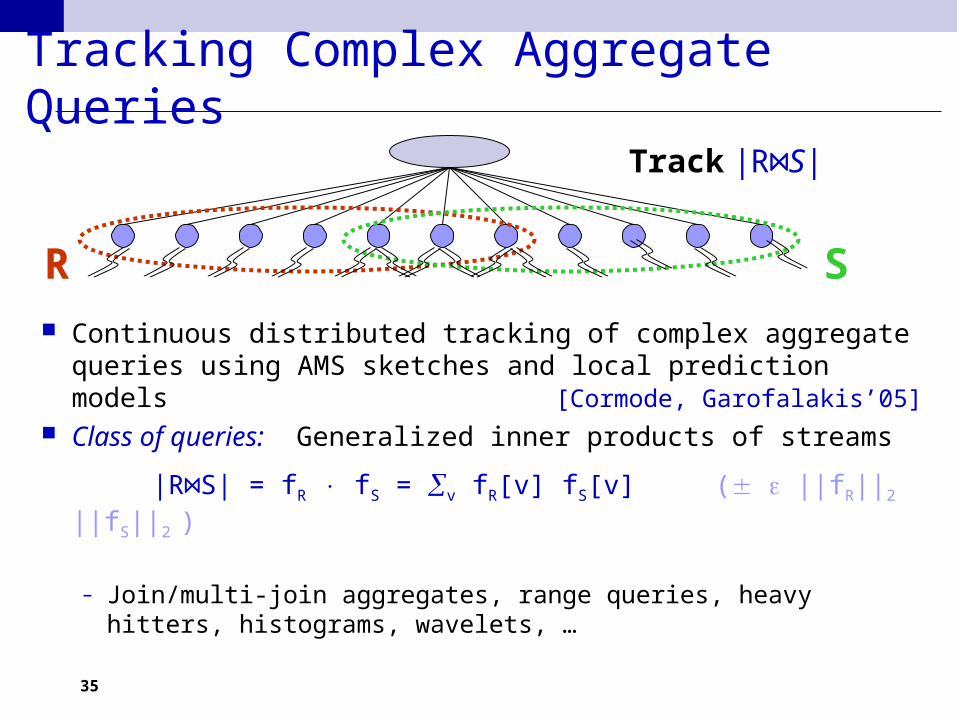
Tracking Complex Aggregate Queries

Continuous distributed tracking of complex aggregate queries using AMS sketches and local prediction models [Cormode, Garofalakis’05]

Class of queries: Generalized inner products of streams

|R S| = f⋈ R fS = v fR[v] fS[v] ( ||fR||2 ||fS||2 )

– Join/multi-join aggregates, range queries, heavy hitters, histograms, wavelets, …

R S

Track |R⋈S|

36

Local Sketches and Sketch Prediction Use (AMS) sketches to summarize local site distributions

– Synopsis=small collection of random linear projections sk(fR,i)

– Linear transform: Simply add to get global stream sketch

Minimize updates to coordinator through Sketch Prediction– Try to predict how local-stream distributions (and their

sketches) will evolve over time– Concise sketch-prediction models, built locally at remote sites

and communicated to coordinator– Shared knowledge on expected stream behavior over time:

Achieve “stability”

37

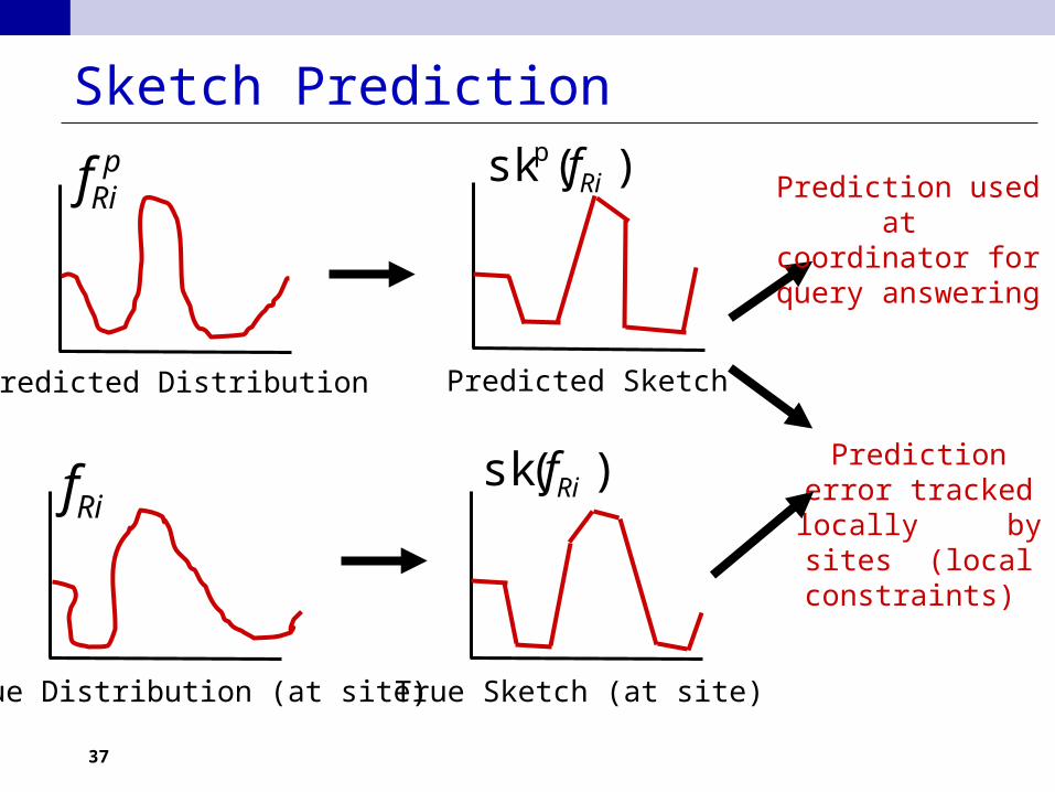
Sketch Prediction

Predicted Distribution Predicted Sketch

True Sketch (at site)

Prediction used at coordinator for query

answering

Prediction error tracked locally

by sites (local constraints)

True Distribution (at site)

Rif

pRif

)(sk Rif

)(skpRif

38

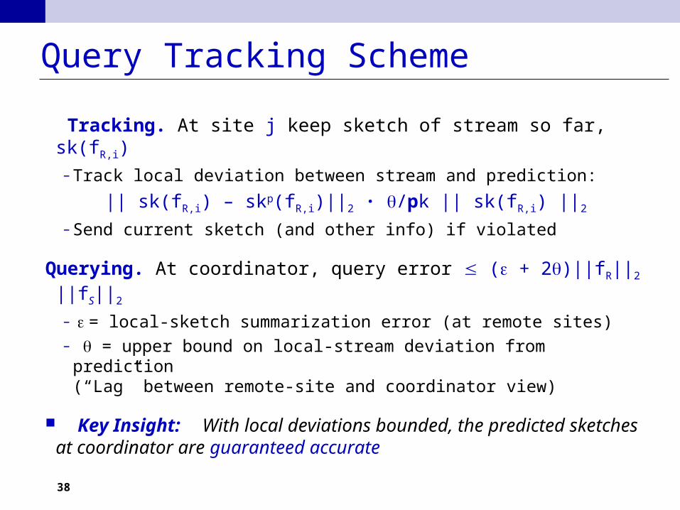
Query Tracking Scheme

Tracking. At site j keep sketch of stream so far, sk(fR,i)– Track local deviation between stream and prediction:

|| sk(fR,i) – skp(fR,i)||2 · /pk || sk(fR,i) ||2– Send current sketch (and other info) if violated

Querying. At coordinator, query error ( + 2)||fR||2 ||fS||2– = local-sketch summarization error (at remote sites) – = upper bound on local-stream deviation from prediction

(“Lag” between remote-site and coordinator view)

Key Insight: With local deviations bounded, the predicted sketches at coordinator are guaranteed accurate

39

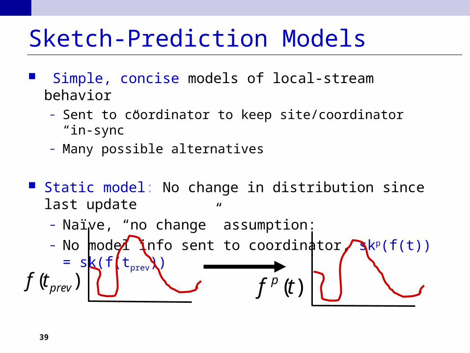
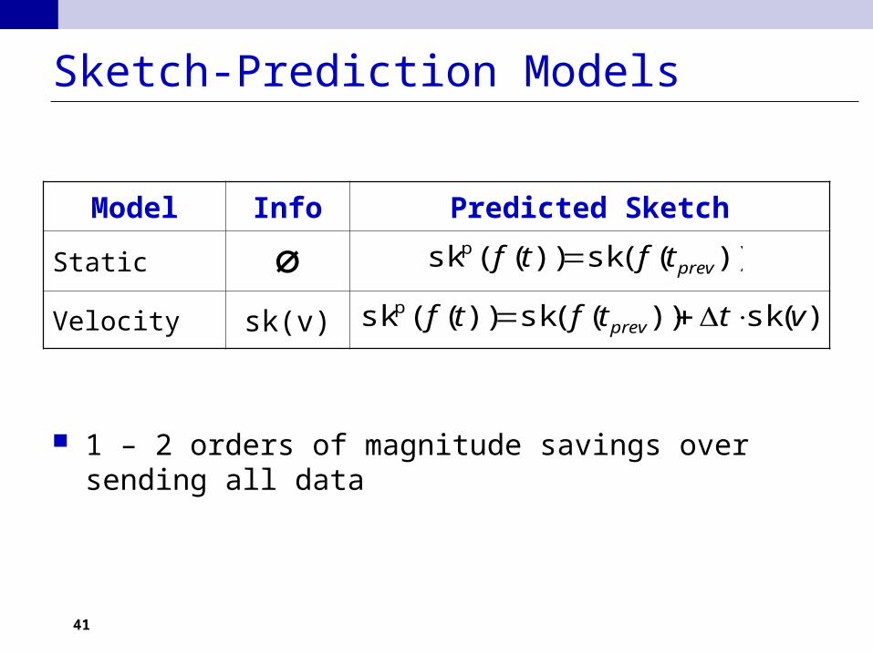
Sketch-Prediction Models

Simple, concise models of local-stream behavior– Sent to coordinator to keep site/coordinator “in-sync” – Many possible alternatives

Static model: No change in distribution since last update– Naïve, “no change” assumption:

– No model info sent to coordinator, skp(f(t)) = sk(f(tprev))

)( prevtf )(tf p

40

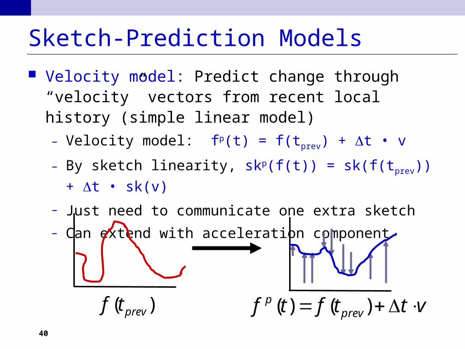
Sketch-Prediction Models Velocity model: Predict change through “velocity” vectors

from recent local history (simple linear model)

– Velocity model: fp(t) = f(tprev) + t • v

– By sketch linearity, skp(f(t)) = sk(f(tprev)) + t • sk(v)

– Just need to communicate one extra sketch – Can extend with acceleration component

)( prevtf vttftf prevp )()(

41

Model Info Predicted Sketch

Static ∅

Velocity sk(v)

Sketch-Prediction Models

1 – 2 orders of magnitude savings over sending all data

)())(())(( vttftf prev skskskp

))(())(( prevtftf skskp

42

Lessons, Thoughts, and Extensions

Dynamic prediction models are a natural choice for continuous in-network processing– Can capture complex temporal (and spatial) patterns to

reduce communication

Many model choices possible – Need to carefully balance power & conciseness– Principled way for model selection?

General-purpose solution (generality of AMS sketch)– Better solutions for special queries

E.g., continuous quantiles [Cormode et al.’05]

43

Conclusions Many new problems posed by developing technologies Common features of distributed streams allow for general

techniques/principles instead of “point” solutions– In-network query processing

Local filtering at sites, trading-off approximation with processing/network costs, …

– Models of “normal” operationStatic, dynamic (“predictive”), probabilistic, …

– Exploiting network locality and avoiding global resyncs

Many new directions unstudied, more will emerge as new technologies arise

Lots of exciting research to be done!