Markov Chains, Graph Spectra, and

Some Static/Dynamic Scaling Limits

Akihito HORA 洞　彰人 (Hokkaido Univ.)

第３回代数的組合せ論「仙台勉強会」

Graduate School of Information Sciences, Tohoku University, 5-6 March 2018

§1 Introduction — algebraic(-combinatoric) vs random structures

§2 Cut-off Phenomenon and Asymptotic Spectral Analysis

§3 Markov Chains on Young Diagrams

§1 Introduction

Interplay between randomness and algebraic(-combinatoric) structure

Algebraic structure plays twofold essential roles:

• produce specific randomness

• give nice tools for analyzing random phenomena

— frameworks of harmonic analysis

(Bose-Mesner algebra, symmetric functions, Kerov-Olshanski algebra, ...)

As probability model,

temporally homogeneous Markov chain on a finite set

(quite simple!)

asymptotic behavior as time (step) →∞recurrence, convergence to invariant distribution, ...

asymptotic behavior as time →∞ and size of state space →∞appropriate scaling in time/space

asymptotic behavior as size of state space →∞

1. Cut-off phenomenon — critical phenomenon in highly symmetric Markov

chain (on group)

2. Interface evolution — Markov chain on Young diagrams (dual object of

symmetric group)

Both probabilistic models show

macroscopic deterministic aspect (law of large numbers)

+ fluctuation (central limit theorem)

§2 Cut-off Phenomenon and Asymptotic Spectral Analysis

§2.1 Markov chain

§2.2 Cut-off phenomenon I: Hamming graph

§2.3 Random walk on association scheme

§2.4 Cut-off phenomenon II

§2.5 Asymptotic spectral analysis (static model) via

quantum decomposition

§3 Markov Chains on Young Diagrams

§3.1 Young graph §3.2 Restriction-induction chain

§3.3 Irreducible characters of Sn §3.4 Kerov-Olshanski algebra

§3.5 Limit shape (static model) §3.6 Interface evolution

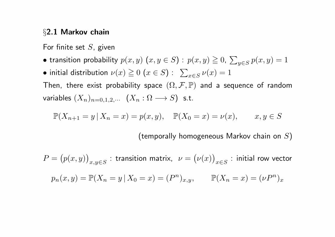
§2.1 Markov chain

For finite set S, given

• transition probability p(x, y) (x, y ∈ S) : p(x, y) ≧ 0,∑

y∈S p(x, y) = 1

• initial distribution ν(x) ≧ 0 (x ∈ S) :∑

x∈S ν(x) = 1

Then, there exist probability space (Ω,F ,P) and a sequence of random

variables (Xn)n=0,1,2,··· (Xn : Ω −→ S) s.t.

P(Xn+1 = y |Xn = x) = p(x, y), P(X0 = x) = ν(x), x, y ∈ S

(temporally homogeneous Markov chain on S)

P =(p(x, y)

)x,y∈S

: transition matrix, ν =(ν(x)

)x∈S

: initial row vector

pn(x, y) = P(Xn = y |X0 = x) = (Pn)x,y, P(Xn = x) = (νPn)x

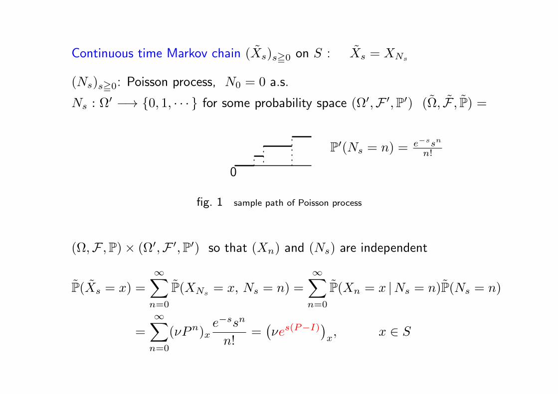
Continuous time Markov chain (Xs)s≧0 on S : Xs = XNs

(Ns)s≧0: Poisson process, N0 = 0 a.s.

Ns : Ω′ −→ 0, 1, · · · for some probability space (Ω′,F ′,P′) (Ω, F , P) =

0

P′(Ns = n) = e−ssn

n!

fig. 1 sample path of Poisson process

(Ω,F ,P)× (Ω′,F ′,P′) so that (Xn) and (Ns) are independent

P(Xs = x) =∞∑

n=0

P(XNs= x, Ns = n) =

∞∑n=0

P(Xn = x |Ns = n)P(Ns = n)

=∞∑

n=0

(νPn)xe−ssn

n!=

(νes(P−I)

)x, x ∈ S

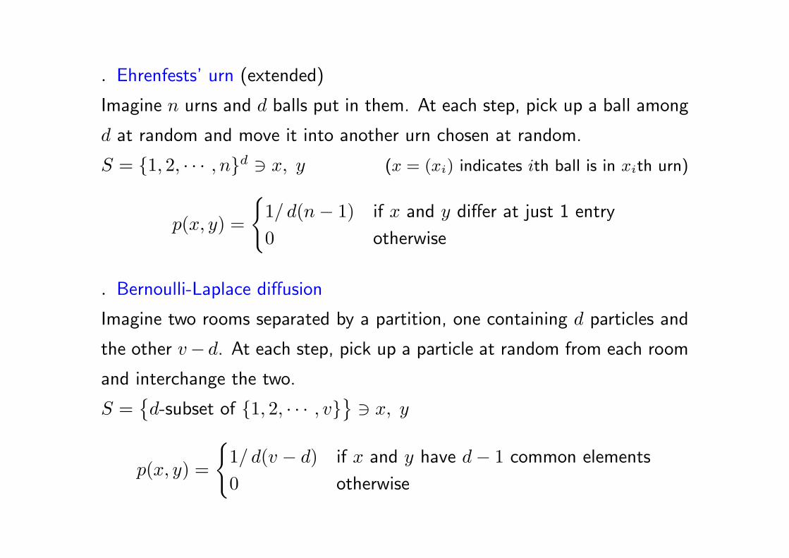
▷ Ehrenfests’ urn (extended)

Imagine n urns and d balls put in them. At each step, pick up a ball among

d at random and move it into another urn chosen at random.

S = 1, 2, · · · , nd ∋ x, y (x = (xi) indicates ith ball is in xith urn)

p(x, y) =

1/ d(n− 1) if x and y differ at just 1 entry

0 otherwise

▷ Bernoulli-Laplace diffusion

Imagine two rooms separated by a partition, one containing d particles and

the other v− d. At each step, pick up a particle at random from each room

and interchange the two.

S =d-subset of 1, 2, · · · , v

∋ x, y

p(x, y) =

1/ d(v − d) if x and y have d− 1 common elements

0 otherwise

§2.2 Cut-off phenomenon I: Hamming graph

Illustrate the cut-off phenomenon — certain critical phenomenon for Markov

chain in which the process of convergence to stationarity is remarkable.

Ehrenfests’ urn (simple random walk on Hamming graph) is a perfect model!

Hamming graph H(d, n) :

vertex sets S = 1, 2, · · · , nd

For x = (xi), y = (yi) ∈ S, ∂(x, y) = ♯ of (i’s s.t. xi = yi).

adjacency matrix Ax,y =

1, ∂(x, y) = 1

0, ∂(x, y) = 1,

valency κ = d(n− 1)

transition matrix P =1

κA

=⇒ simple random walk on S with uniform invariant distribution

For continuous time simple random walk on H(d, n),

(es(P−I))x, · : distribution at time s starting from x

total variation distance between distributions at time s and ∞

D(d,n)(s) =1

2

∥∥(es(P−I))x, · − (uniform distribution)∥∥tot

=1

2

∑y∈S

∣∣∣(es(P−I))x,y −1

nd

∣∣∣(independent of starting vertex x)

D(0) = 1− 1

nd≈ 1, D(∞) = 0

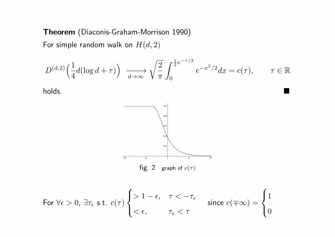
Theorem (Diaconis-Graham-Morrison 1990)

For simple random walk on H(d, 2)

D(d,2)(14d(log d+ τ)

)−−−→d→∞

√2

π

∫ 12 e

−τ/2

0

e−x2/2dx = c(τ), τ ∈ R

holds.

fig. 2 graph of c(τ)

For ∀ϵ > 0, ∃τϵ s.t. c(τ)

> 1− ϵ, τ < −τϵ

< ϵ, τϵ < τsince c(∓∞) =

1

0

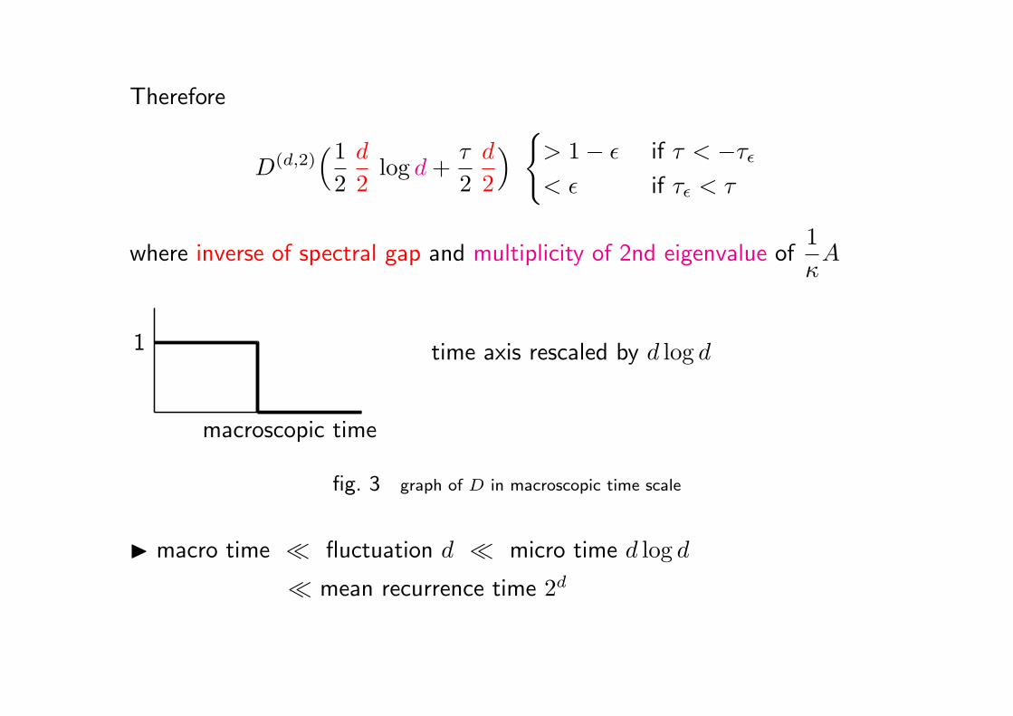
Therefore

D(d,2)(12

d

2log d+

τ

2

d

2

) > 1− ϵ if τ < −τϵ< ϵ if τϵ < τ

where inverse of spectral gap and multiplicity of 2nd eigenvalue of1

κA

1

macroscopic time

time axis rescaled by d log d

fig. 3 graph of D in macroscopic time scale

macro time ≪ fluctuation d ≪ micro time d log d

≪ mean recurrence time 2d

§2.3 Random walk on association scheme

large multiplicity (degeneration) of 2nd eigenvalue of transition matrix

⇐= high symmetry for Markov chain ⇐= “random walk”

Let group G act on S transitively, S ∼= G/K, and

p(gx, gy) = p(x, y), x, y ∈ S, g ∈ G.

Then ∃µ ∈ P(K\G/K) s.t. P = µ ∗ · (convolution operator), i.e.

the Markov chain is product of independent G-valued random variables with

K-bi-invariant distribution

“ random walk ⇐⇒ spatially symmetric Markov chain”

Natural and fruitful extension is

“ random walk ⇐⇒ transition matrix belongs to Bose-Mesner algebra of

association scheme”

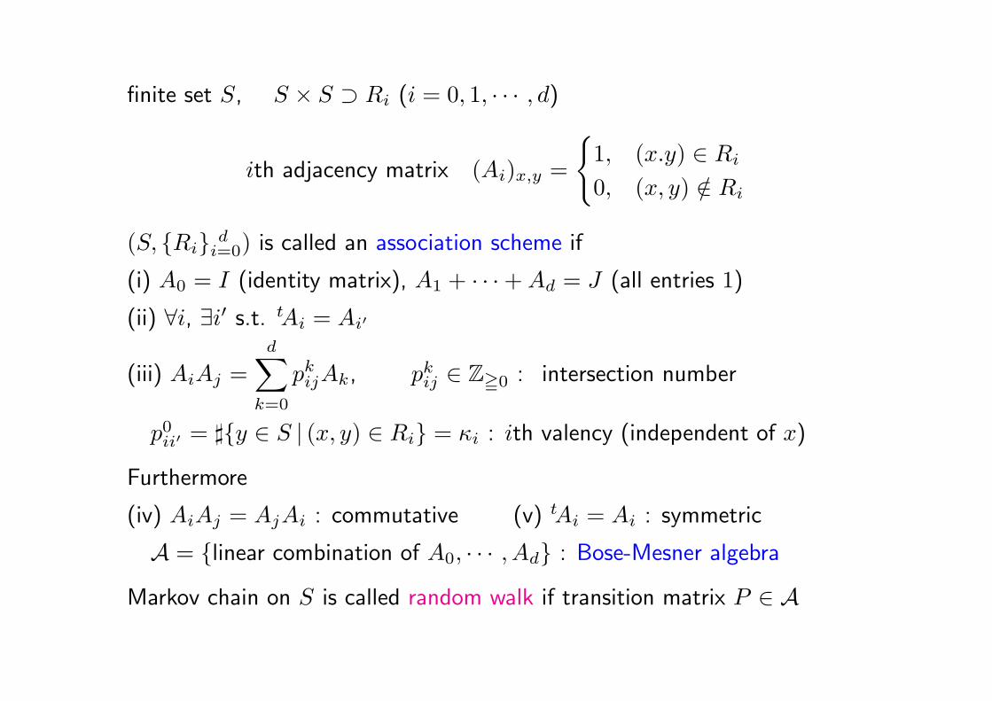
finite set S, S × S ⊃ Ri (i = 0, 1, · · · , d)

ith adjacency matrix (Ai)x,y =

1, (x.y) ∈ Ri

0, (x, y) /∈ Ri

(S, Ri di=0) is called an association scheme if

(i) A0 = I (identity matrix), A1 + · · ·+Ad = J (all entries 1)

(ii) ∀i, ∃i′ s.t. tAi = Ai′

(iii) AiAj =d∑

k=0

pkijAk, pkij ∈ Z≧0 : intersection number

p0ii′ = ♯y ∈ S | (x, y) ∈ Ri = κi : ith valency (independent of x)

Furthermore

(iv) AiAj = AjAi : commutative (v) tAi = Ai : symmetric

A = linear combination of A0, · · · , Ad : Bose-Mesner algebra

Markov chain on S is called random walk if transition matrix P ∈ A

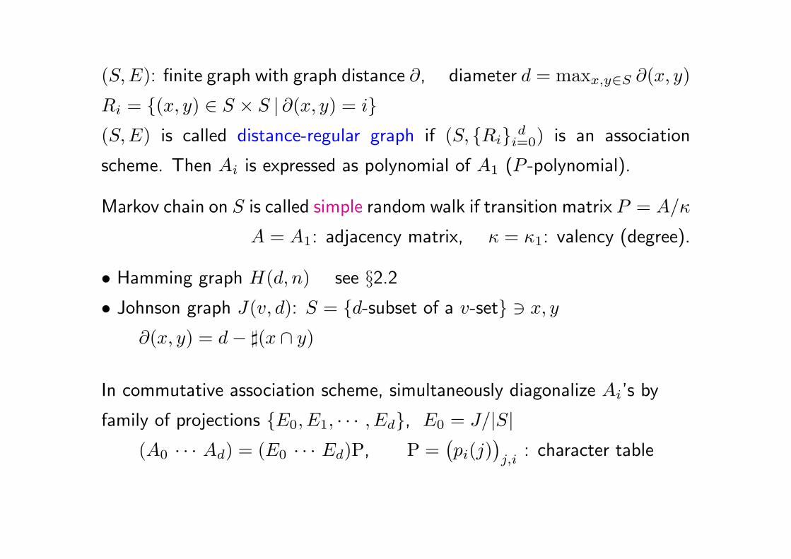
(S,E): finite graph with graph distance ∂, diameter d = maxx,y∈S ∂(x, y)

Ri = (x, y) ∈ S × S | ∂(x, y) = i(S,E) is called distance-regular graph if (S, Ri d

i=0) is an association

scheme. Then Ai is expressed as polynomial of A1 (P -polynomial).

Markov chain on S is called simple random walk if transition matrix P = A/κ

A = A1: adjacency matrix, κ = κ1: valency (degree).

• Hamming graph H(d, n) see §2.2• Johnson graph J(v, d): S = d-subset of a v-set ∋ x, y

∂(x, y) = d− ♯(x ∩ y)

In commutative association scheme, simultaneously diagonalize Ai’s by

family of projections E0, E1, · · · , Ed, E0 = J/|S|(A0 · · · Ad) = (E0 · · · Ed)P, P =

(pi(j)

)j,i

: character table

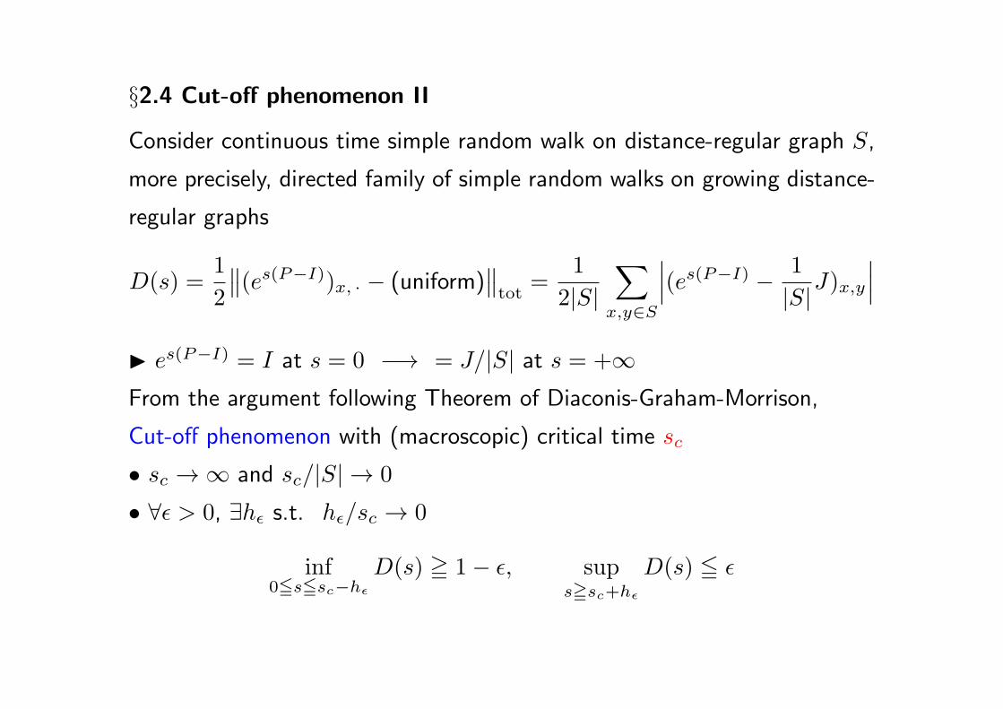
§2.4 Cut-off phenomenon II

Consider continuous time simple random walk on distance-regular graph S,

more precisely, directed family of simple random walks on growing distance-

regular graphs

D(s) =1

2

∥∥(es(P−I))x, · − (uniform)∥∥tot

=1

2|S|∑

x,y∈S

∣∣∣(es(P−I) − 1

|S|J)x,y

∣∣∣ es(P−I) = I at s = 0 −→ = J/|S| at s = +∞From the argument following Theorem of Diaconis-Graham-Morrison,

Cut-off phenomenon with (macroscopic) critical time sc

• sc →∞ and sc/|S| → 0

• ∀ϵ > 0, ∃hϵ s.t. hϵ/sc → 0

inf0≦s≦sc−hϵ

D(s) ≧ 1− ϵ, sups≧sc+hϵ

D(s) ≦ ϵ

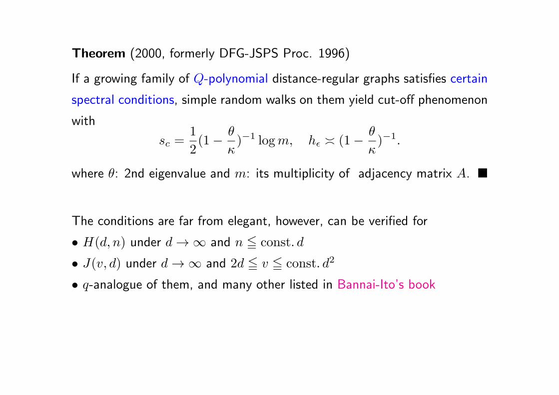
Theorem (2000, formerly DFG-JSPS Proc. 1996)

If a growing family of Q-polynomial distance-regular graphs satisfies certain

spectral conditions, simple random walks on them yield cut-off phenomenon

with

sc =1

2(1− θ

κ)−1 logm, hϵ ≍ (1− θ

κ)−1.

where θ: 2nd eigenvalue and m: its multiplicity of adjacency matrix A.

The conditions are far from elegant, however, can be verified for

• H(d, n) under d→∞ and n ≦ const. d

• J(v, d) under d→∞ and 2d ≦ v ≦ const. d2

• q-analogue of them, and many other listed in Bannai-Ito’s book

Role of symmetry

• give rise to degeneration of eigenvalues

(eigenspace invariant w.r.t. actions)

• put transition matrix into Bose-Mesner algebra =⇒ functional calculus

(characters, spherical functions, · · · help diagonalizing transition matrix)

Other models of cut-off phenomenon

⋆ card shuffling : random walk on symmetric group with various generators

(= various Cayley graphs)

⋆ framework of hypergroup (finite Gelfand pair, spherical dual) etc.

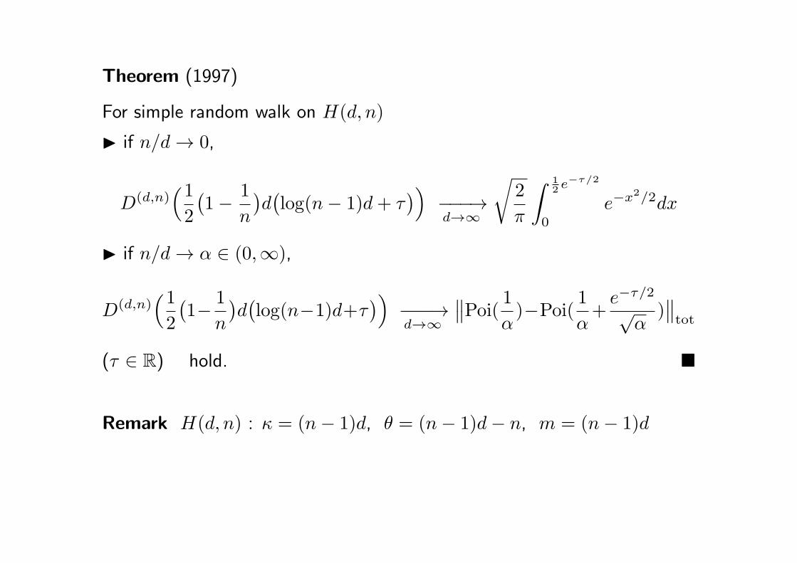
Theorem (1997)

For simple random walk on H(d, n)

if n/d→ 0,

D(d,n)(12

(1− 1

n

)d(log(n− 1)d+ τ

))−−−→d→∞

√2

π

∫ 12 e

−τ/2

0

e−x2/2dx

if n/d→ α ∈ (0,∞),

D(d,n)(12

(1− 1

n

)d(log(n−1)d+τ

))−−−→d→∞

∥∥Poi( 1α)−Poi( 1

α+e−τ/2

√α

)∥∥tot

(τ ∈ R) hold.

Remark H(d, n) : κ = (n− 1)d, θ = (n− 1)d− n, m = (n− 1)d

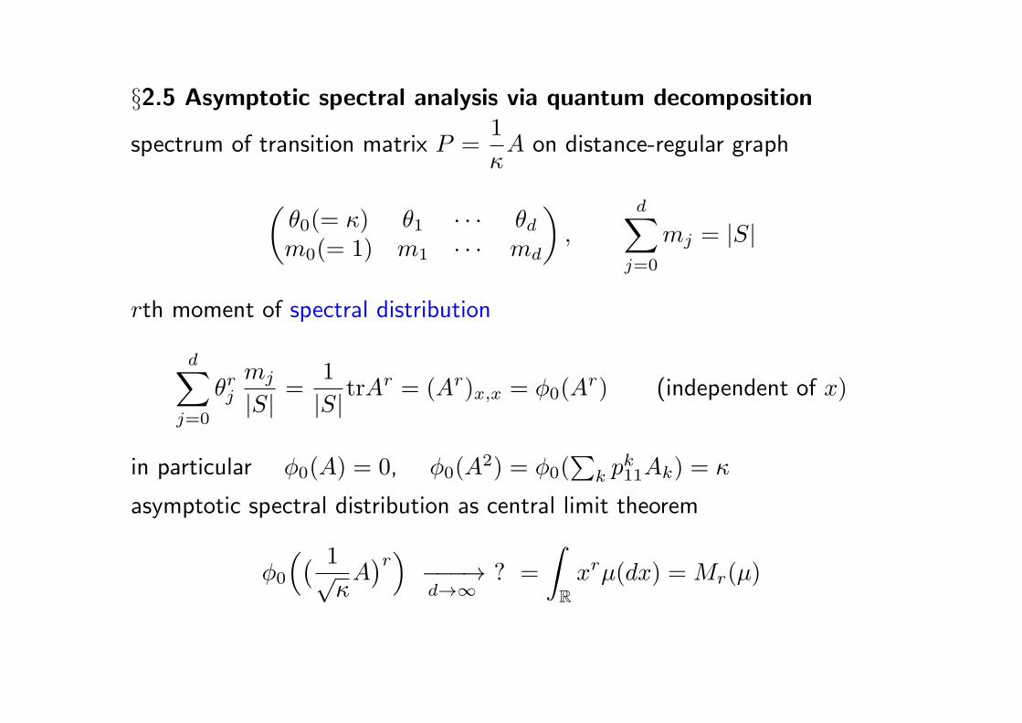
§2.5 Asymptotic spectral analysis via quantum decomposition

spectrum of transition matrix P =1

κA on distance-regular graph

(θ0(= κ) θ1 · · · θdm0(= 1) m1 · · · md

),

d∑j=0

mj = |S|

rth moment of spectral distribution

d∑j=0

θrjmj

|S|=

1

|S|trAr = (Ar)x,x = ϕ0(A

r) (independent of x)

in particular ϕ0(A) = 0, ϕ0(A2) = ϕ0(

∑k p

k11Ak) = κ

asymptotic spectral distribution as central limit theorem

ϕ0

(( 1√κA)r) −−−→

d→∞? =

∫Rxrµ(dx) = Mr(µ)

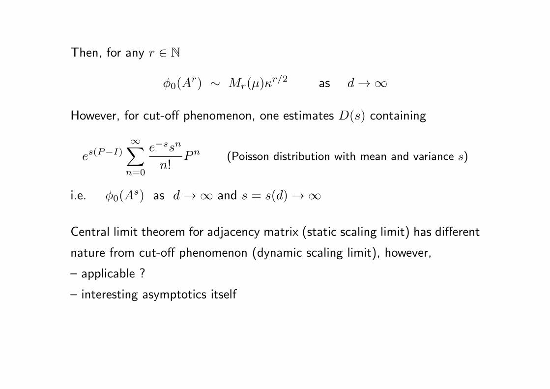
Then, for any r ∈ N

ϕ0(Ar) ∼ Mr(µ)κ

r/2 as d→∞

However, for cut-off phenomenon, one estimates D(s) containing

es(P−I)∞∑

n=0

e−ssn

n!Pn (Poisson distribution with mean and variance s)

i.e. ϕ0(As) as d→∞ and s = s(d)→∞

Central limit theorem for adjacency matrix (static scaling limit) has different

nature from cut-off phenomenon (dynamic scaling limit), however,

– applicable ?

– interesting asymptotics itself

Viewpoint of quantum probability

• quantum decomposition A = A+ +A− (+Ao)

with certain commutation relation

• limit picture drawn by creation/annihilation operators on appropriate

Fock space

• other state than (vacuum) ϕ0

Hashimoto-Obata-Tabei (2001) : for Hamming graph by using Hermite

polynomial, Gauss measure, Boson Fock space

Collaboration with Obata school · · ·

A. Hora, N. Obata: Quantum Probability and Spectral Analysis of Graphs,

Theoretical and Mathematical Physics, Springer, 2007

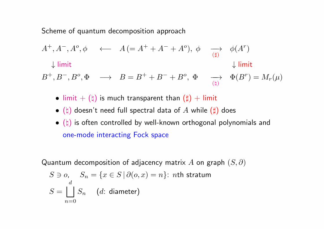
Scheme of quantum decomposition approach

A+, A−, Ao, ϕ ←− A (= A+ +A− +Ao), ϕ −−→(♯)

ϕ(Ar)

↓ limit ↓ limit

B+, B−, Bo,Φ −→ B = B+ +B− +Bo, Φ −−→()

Φ(Br) = Mr(µ)

• limit + () is much transparent than (♯) + limit

• () doesn’t need full spectral data of A while (♯) does

• () is often controlled by well-known orthogonal polynomials and

one-mode interacting Fock space

Quantum decomposition of adjacency matrix A on graph (S, ∂)

S ∋ o, Sn = x ∈ S | ∂(o, x) = n: nth stratum

S =

d⊔n=0

Sn (d: diameter)

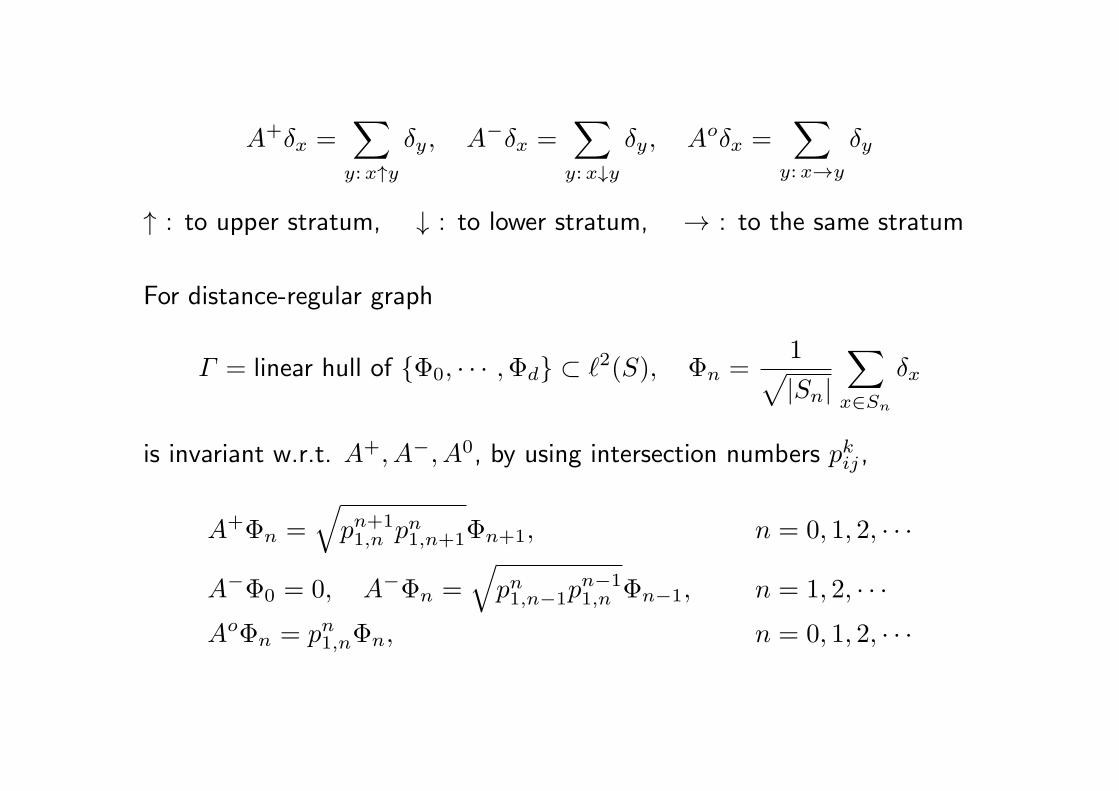
A+δx =∑y: x↑y

δy, A−δx =∑y: x↓y

δy, Aoδx =∑

y: x→y

δy

↑ : to upper stratum, ↓ : to lower stratum, → : to the same stratum

For distance-regular graph

Γ = linear hull of Φ0, · · · ,Φd ⊂ ℓ2(S), Φn =1√|Sn|

∑x∈Sn

δx

is invariant w.r.t. A+, A−, A0, by using intersection numbers pkij ,

A+Φn =√

pn+11,n pn1,n+1Φn+1, n = 0, 1, 2, · · ·

A−Φ0 = 0, A−Φn =√

pn1,n−1pn−11,n Φn−1, n = 1, 2, · · ·

AoΦn = pn1,nΦn, n = 0, 1, 2, · · ·

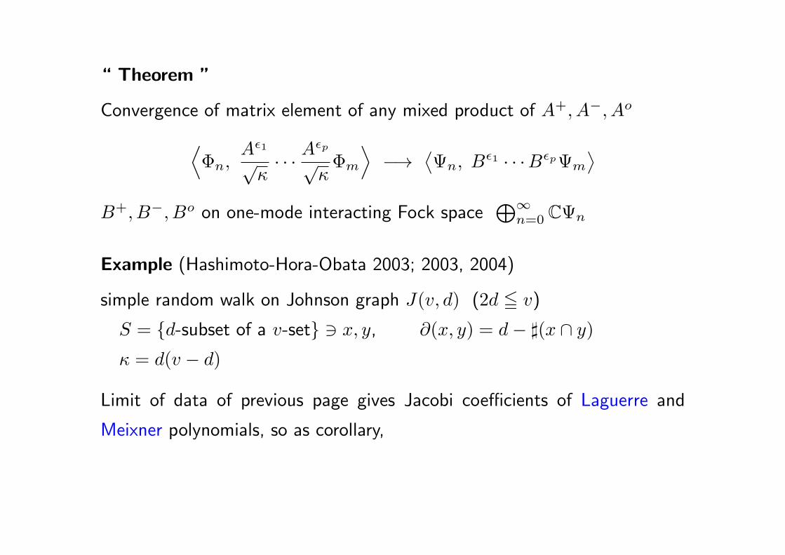
“ Theorem ”

Convergence of matrix element of any mixed product of A+, A−, Ao

⟨Φn,

Aϵ1

√κ· · · A

ϵp

√κΦm

⟩−→

⟨Ψn, B

ϵ1 · · ·BϵpΨm

⟩B+, B−, Bo on one-mode interacting Fock space

⊕∞n=0 CΨn

Example (Hashimoto-Hora-Obata 2003; 2003, 2004)

simple random walk on Johnson graph J(v, d) (2d ≦ v)

S = d-subset of a v-set ∋ x, y, ∂(x, y) = d− ♯(x ∩ y)

κ = d(v − d)

Limit of data of previous page gives Jacobi coefficients of Laguerre and

Meixner polynomials, so as corollary,

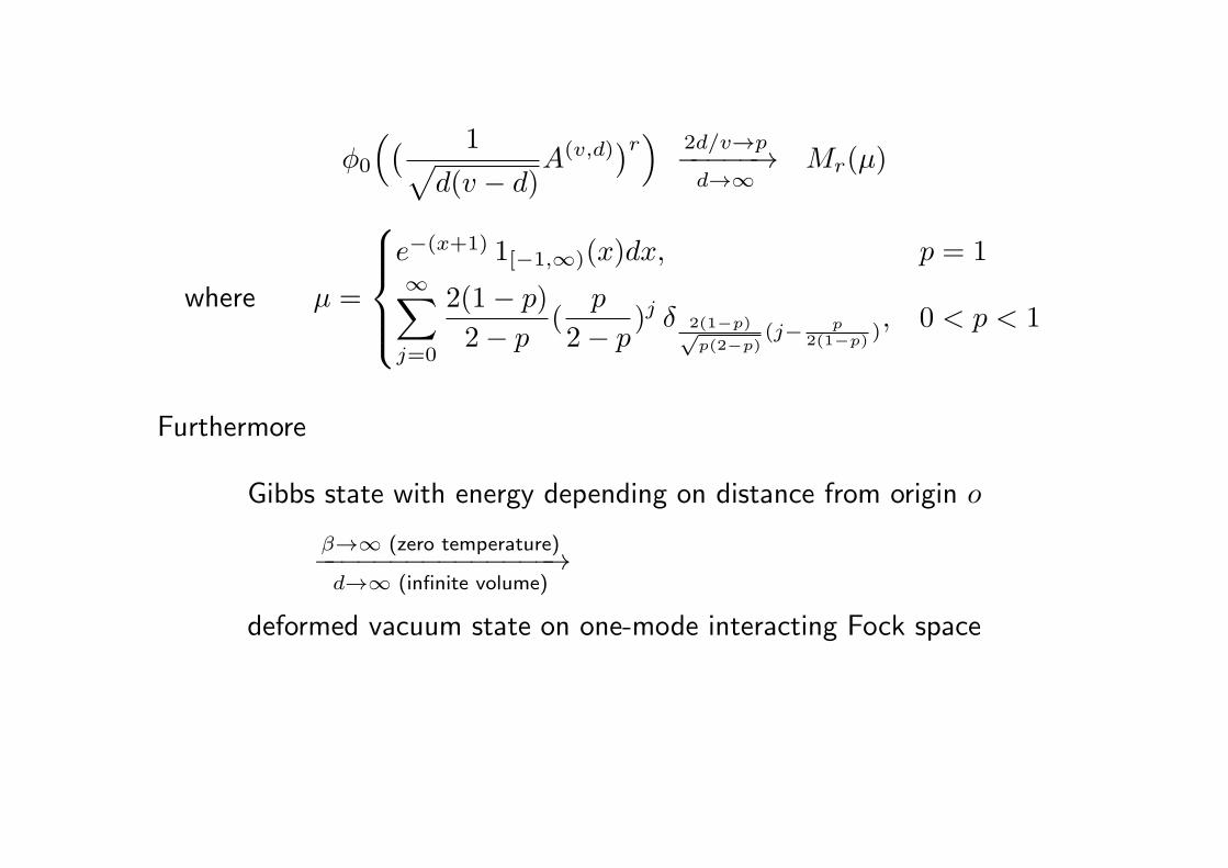
ϕ0

(( 1√d(v − d)

A(v,d))r) 2d/v→p−−−−−→

d→∞Mr(µ)

where µ =

e−(x+1) 1[−1,∞)(x)dx, p = 1∞∑j=0

2(1− p)

2− p(

p

2− p)j δ 2(1−p)√

p(2−p)(j− p

2(1−p)), 0 < p < 1

Furthermore

Gibbs state with energy depending on distance from origin o

β→∞ (zero temperature)−−−−−−−−−−−−−−−→d→∞ (infinite volume)

deformed vacuum state on one-mode interacting Fock space

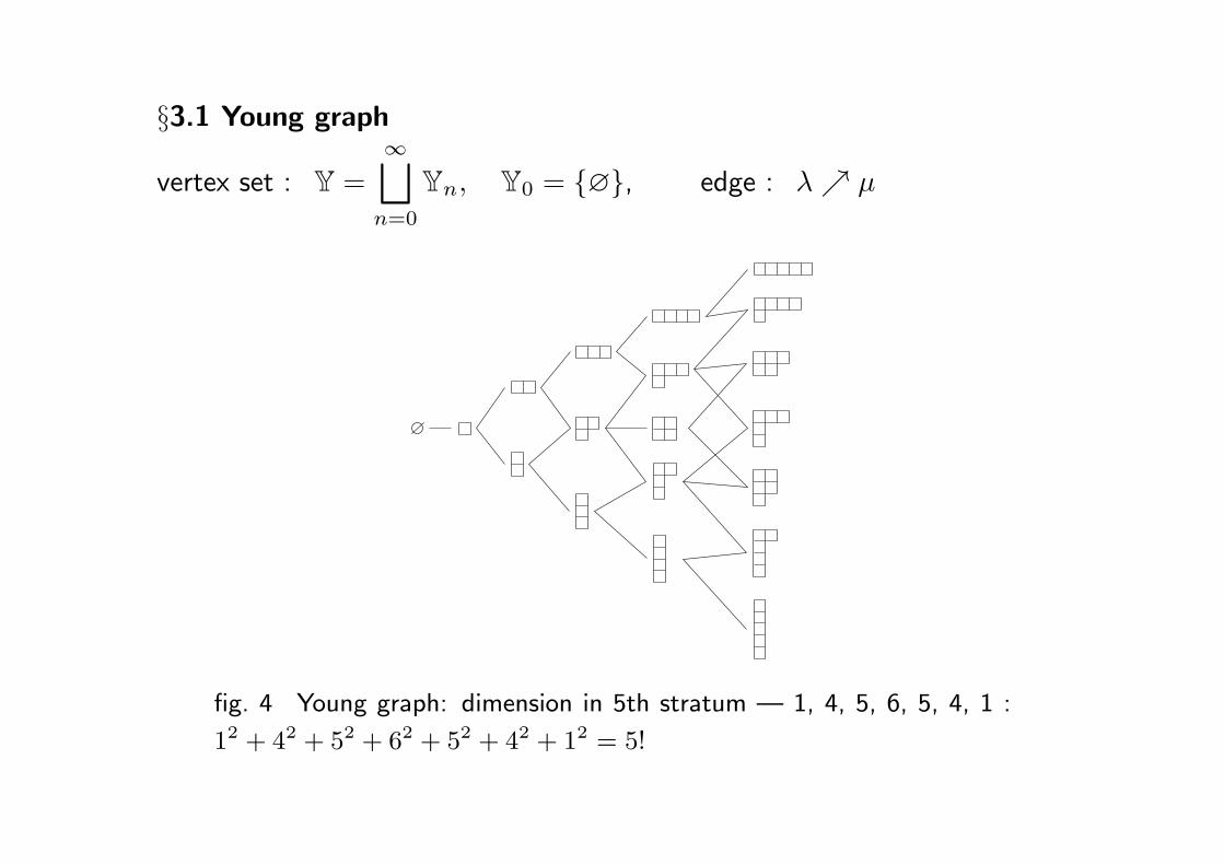
§3.1 Young graph

vertex set : Y =

∞⊔n=0

Yn, Y0 = ∅, edge : λ µ

fig. 4 Young graph: dimension in 5th stratum — 1, 4, 5, 6, 5, 4, 1 :

12 + 42 + 52 + 62 + 52 + 42 + 12 = 5!

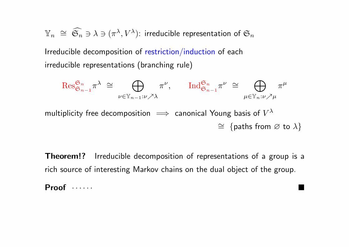
Yn∼= Sn ∋ λ ∋ (πλ, V λ): irreducible representation of Sn

Irreducible decomposition of restriction/induction of each

irreducible representations (branching rule)

ResSn

Sn−1πλ ∼=

⊕ν∈Yn−1:νλ

πν , IndSn

Sn−1πν ∼=

⊕µ∈Yn:νµ

πµ

multiplicity free decomposition =⇒ canonical Young basis of V λ

∼= paths from ∅ to λ

Theorem!? Irreducible decomposition of representations of a group is a

rich source of interesting Markov chains on the dual object of the group.

Proof · · · · · ·

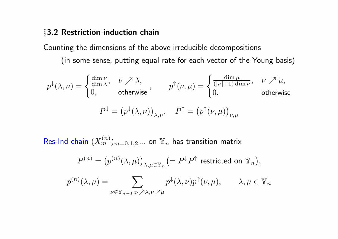
§3.2 Restriction-induction chain

Counting the dimensions of the above irreducible decompositions

(in some sense, putting equal rate for each vector of the Young basis)

p↓(λ, ν) =

dim νdimλ , ν λ,

0, otherwise, p↑(ν, µ) =

dimµ

(|ν|+1) dim ν , ν µ,

0, otherwise

P ↓ =(p↓(λ, ν)

)λ,ν

, P ↑ =(p↑(ν, µ)

)ν,µ

Res-Ind chain (X(n)m )m=0,1,2,··· on Yn has transition matrix

P (n) =(p(n)(λ, µ)

)λ,µ∈Yn

(= P ↓P ↑ restricted on Yn

),

p(n)(λ, µ) =∑

ν∈Yn−1:νλ,νµ

p↓(λ, ν)p↑(ν, µ), λ, µ ∈ Yn

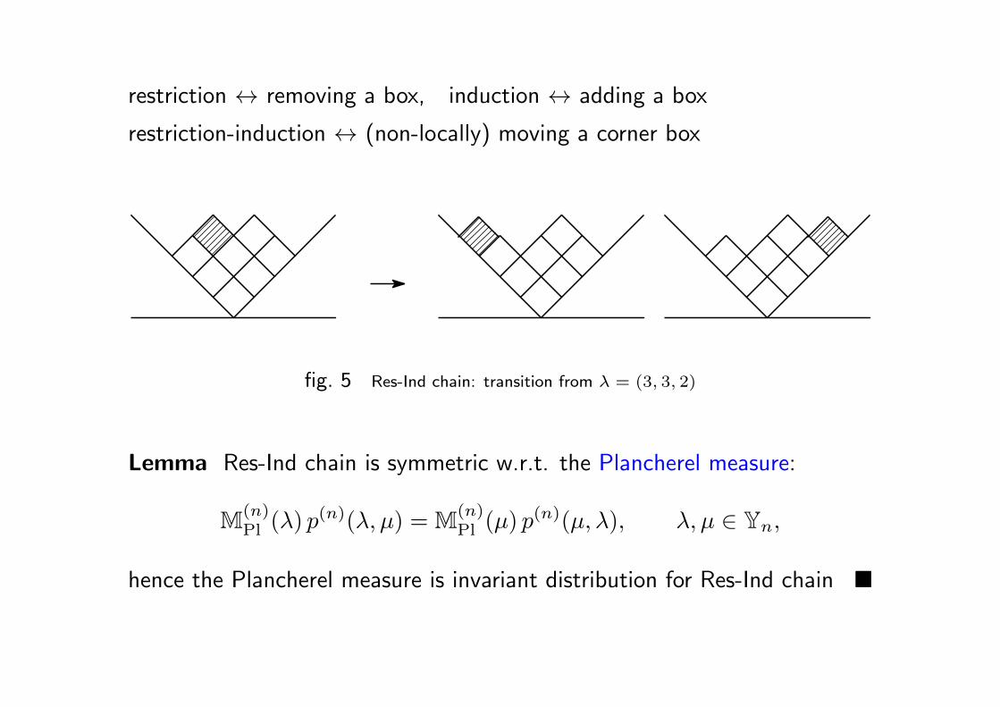
restriction ↔ removing a box, induction ↔ adding a box

restriction-induction ↔ (non-locally) moving a corner box

fig. 5 Res-Ind chain: transition from λ = (3, 3, 2)

Lemma Res-Ind chain is symmetric w.r.t. the Plancherel measure:

M(n)Pl (λ) p

(n)(λ, µ) = M(n)Pl (µ) p

(n)(µ, λ), λ, µ ∈ Yn,

hence the Plancherel measure is invariant distribution for Res-Ind chain

▷ Plancherel measure on Yn is

M(n)Pl (λ) =

(dimλ)2

n!

(← Plancherel formula for Fourier transform on Sn)

▷ Markov chain (Zn) on the Young graph with initial distribution δ∅ and

transition matrix P ↑ is called the Plancherel growth process.

The distribution after n step is P(Zn = λ) =(dimλ)2

n!= M(n)

Pl (λ)

Continuous time Res-Ind chain X(n)s = X

(n)Ns

on Yn (Ns: Poisson process)

• transition matrix es(P(n)−I)

• invariant distribution M(n)Pl

§3.3 Irreducible characters of symmetric group

P (n) = (P ↓P ↑)|Yn: transition matrix of Res-Ind chain on Yn

Diagonalize P (n) by using irreducible characters of Sn

(generally available for non-multiplicity-free branching rule also)

For representation (π, V ), χ(x) = trπ(x) χ = χ/dimV

Yn parametrizes both the equivalence classes of irreducible representations

and the conjugacy classes of Sn

Character table (χλρ)ρ,λ∈Yn

Dual approach in asymptotic theory — fix ρ, then |λ| → ∞ i.e. consider

χλ(ρ,1n−k), ρ ∈ Yk, λ ∈ Yn, k ≦ n

where (ρ, 1n−k) = ρ ⊔ (1n−k) ∈ Yn so that one can let n→∞

Lemma For |ρ| ≦ n s.t. ρ = (1m1(ρ)2m2(ρ) · · · ),

P (n)(χλ(ρ,1n−|ρ|)

)λ∈Yn

=(1− |ρ| −m1(ρ)

n

)(χλ(ρ,1n−|ρ|)

)λ∈Yn

where ( · )λ∈Ynis a column vector

For transition matrix of continuous time Res-Ind chain,

es(P(n)−I)

(χλ(ρ,1n−|ρ|)

)λ∈Yn

= e−(|ρ|−m1(ρ))s/n(χλ(ρ,1n−|ρ|)

)λ∈Yn

Letting ν be an initial distribution on Yn,

P(X(n)s = λ) = PX(n)

s (λ) =(νes(P

(n)−I))λ, λ ∈ Yn

Expectation of irreducible character w.r.t. initial distribution

=⇒ w.r.t. the distribution at time s

§3.4 Kerov-Olshanski algebra

Irreducible characters are (one of) the most important random variables to

analyze group-theoretical ensemble of Young diagrams.

For k = |ρ| ≦ |λ| = n, set a function on Y

Σρ(λ) = n(n− 1) · · · (n− k + 1)χλ(ρ,1n−k) (= 0 if k > n)

For one row diagram ρ = (k), Σk = Σ(k)

▷ A = linear combination of Σρ | ρ ∈ Y : Kerov–Olshanski algebra

Considering A as an algebra of random variables, one can compute many

things about random Young diagrams.

Coordinates for a Young diagram −→ element of A as a polynomial function

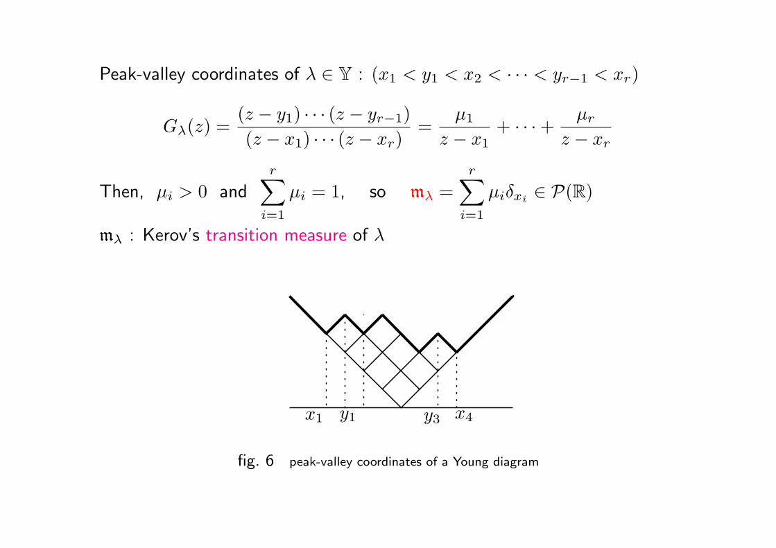
Peak-valley coordinates of λ ∈ Y : (x1 < y1 < x2 < · · · < yr−1 < xr)

Gλ(z) =(z − y1) · · · (z − yr−1)

(z − x1) · · · (z − xr)=

µ1

z − x1+ · · ·+ µr

z − xr

Then, µi > 0 andr∑

i=1

µi = 1, so mλ =

r∑i=1

µiδxi ∈ P(R)

mλ : Kerov’s transition measure of λ

x1 y1 x4y3

fig. 6 peak-valley coordinates of a Young diagram

Gλ(z) =

∫R

1

z − xmλ(dx) =

∞∑n=0

1

zn+1

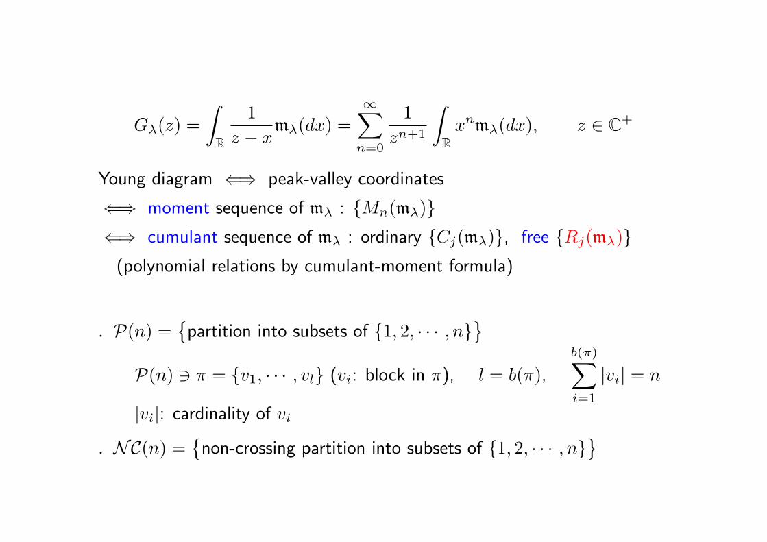
∫Rxnmλ(dx), z ∈ C+

Young diagram ⇐⇒ peak-valley coordinates

⇐⇒ moment sequence of mλ : Mn(mλ)⇐⇒ cumulant sequence of mλ : ordinary Cj(mλ), free Rj(mλ)(polynomial relations by cumulant-moment formula)

▷ P(n) =partition into subsets of 1, 2, · · · , n

P(n) ∋ π = v1, · · · , vl (vi: block in π), l = b(π),

b(π)∑i=1

|vi| = n

|vi|: cardinality of vi

▷ NC(n) =non-crossing partition into subsets of 1, 2, · · · , n

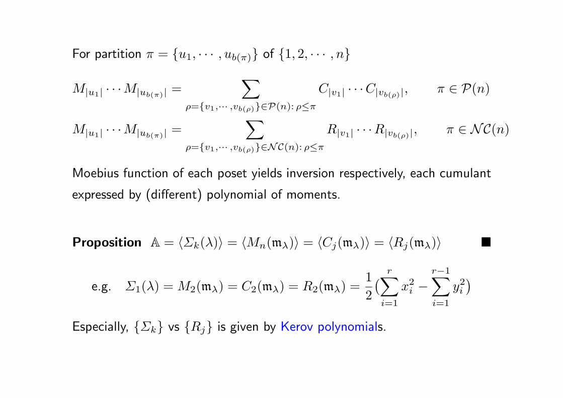
For partition π = u1, · · · , ub(π) of 1, 2, · · · , n

M|u1| · · ·M|ub(π)| =∑

ρ=v1,··· ,vb(ρ)∈P(n): ρ≤π

C|v1| · · ·C|vb(ρ)|, π ∈ P(n)

M|u1| · · ·M|ub(π)| =∑

ρ=v1,··· ,vb(ρ)∈NC(n): ρ≤π

R|v1| · · ·R|vb(ρ)|, π ∈ NC(n)

Moebius function of each poset yields inversion respectively, each cumulant

expressed by (different) polynomial of moments.

Proposition A = ⟨Σk(λ)⟩ = ⟨Mn(mλ)⟩ = ⟨Cj(mλ)⟩ = ⟨Rj(mλ)⟩

e.g. Σ1(λ) = M2(mλ) = C2(mλ) = R2(mλ) =1

2

( r∑i=1

x2i −

r−1∑i=1

y2i)

Especially, Σk vs Rj is given by Kerov polynomials.

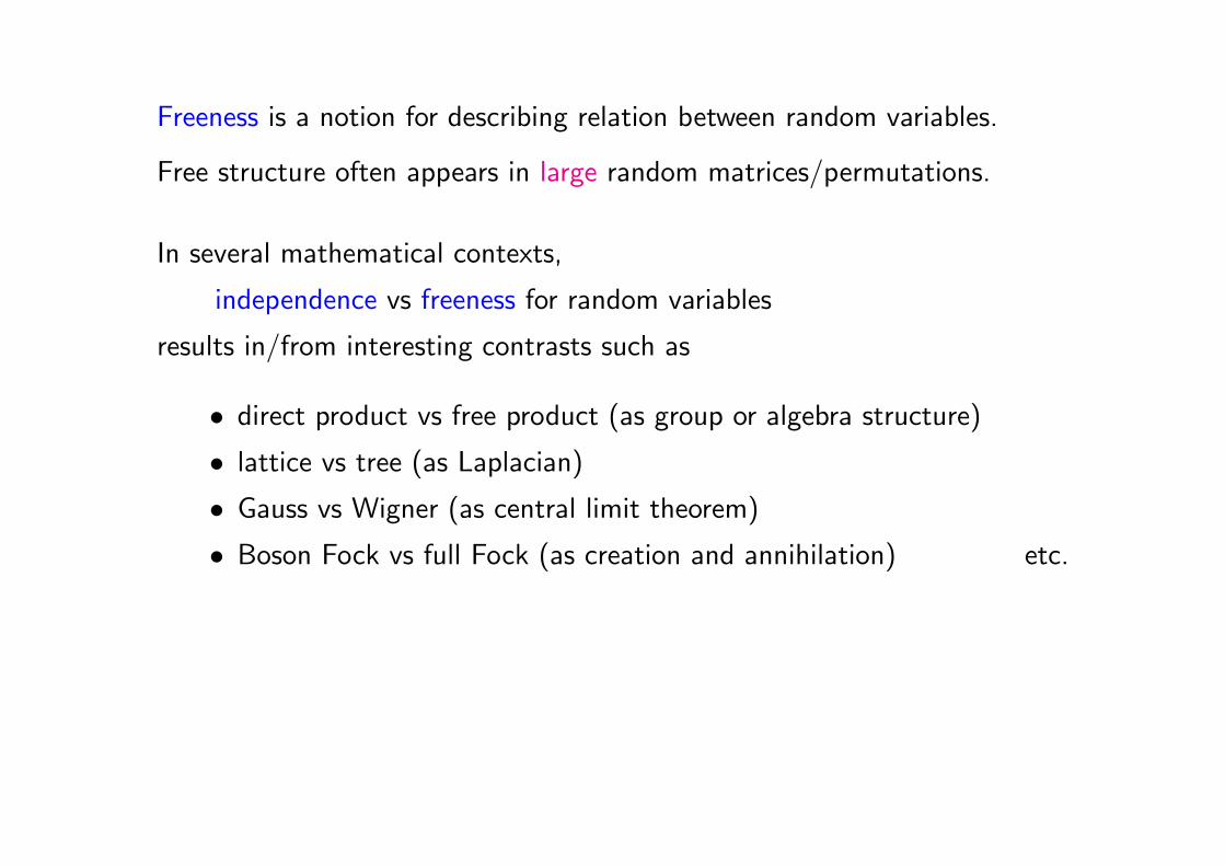
Freeness is a notion for describing relation between random variables.

Free structure often appears in large random matrices/permutations.

In several mathematical contexts,

independence vs freeness for random variables

results in/from interesting contrasts such as

• direct product vs free product (as group or algebra structure)

• lattice vs tree (as Laplacian)

• Gauss vs Wigner (as central limit theorem)

• Boson Fock vs full Fock (as creation and annihilation) etc.

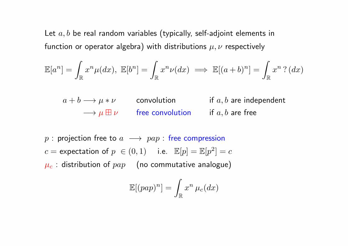
Let a, b be real random variables (typically, self-adjoint elements in

function or operator algebra) with distributions µ, ν respectively

E[an] =∫Rxnµ(dx), E[bn] =

∫Rxnν(dx) =⇒ E[(a+ b)n] =

∫Rxn ? (dx)

a+ b −→ µ ∗ ν convolution if a, b are independent

−→ µ⊞ ν free convolution if a, b are free

p : projection free to a −→ pap : free compression

c = expectation of p ∈ (0, 1) i.e. E[p] = E[p2] = c

µc : distribution of pap (no commutative analogue)

E[(pap)n] =∫Rxn µc(dx)

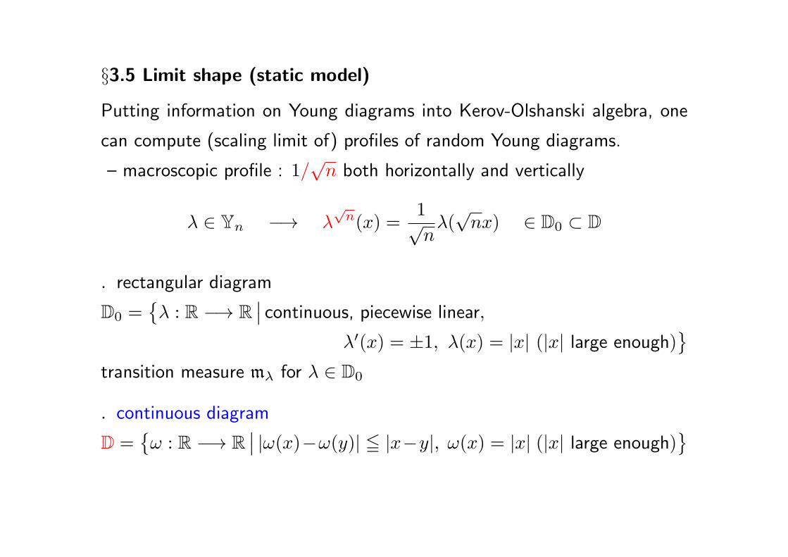
§3.5 Limit shape (static model)

Putting information on Young diagrams into Kerov-Olshanski algebra, one

can compute (scaling limit of) profiles of random Young diagrams.

– macroscopic profile : 1/√n both horizontally and vertically

λ ∈ Yn −→ λ√n(x) =

1√nλ(√nx) ∈ D0 ⊂ D

▷ rectangular diagram

D0 =λ : R −→ R

∣∣ continuous, piecewise linear,

λ′(x) = ±1, λ(x) = |x| (|x| large enough)

transition measure mλ for λ ∈ D0

▷ continuous diagram

D =ω : R −→ R

∣∣ |ω(x)−ω(y)| ≦ |x−y|, ω(x) = |x| (|x| large enough)

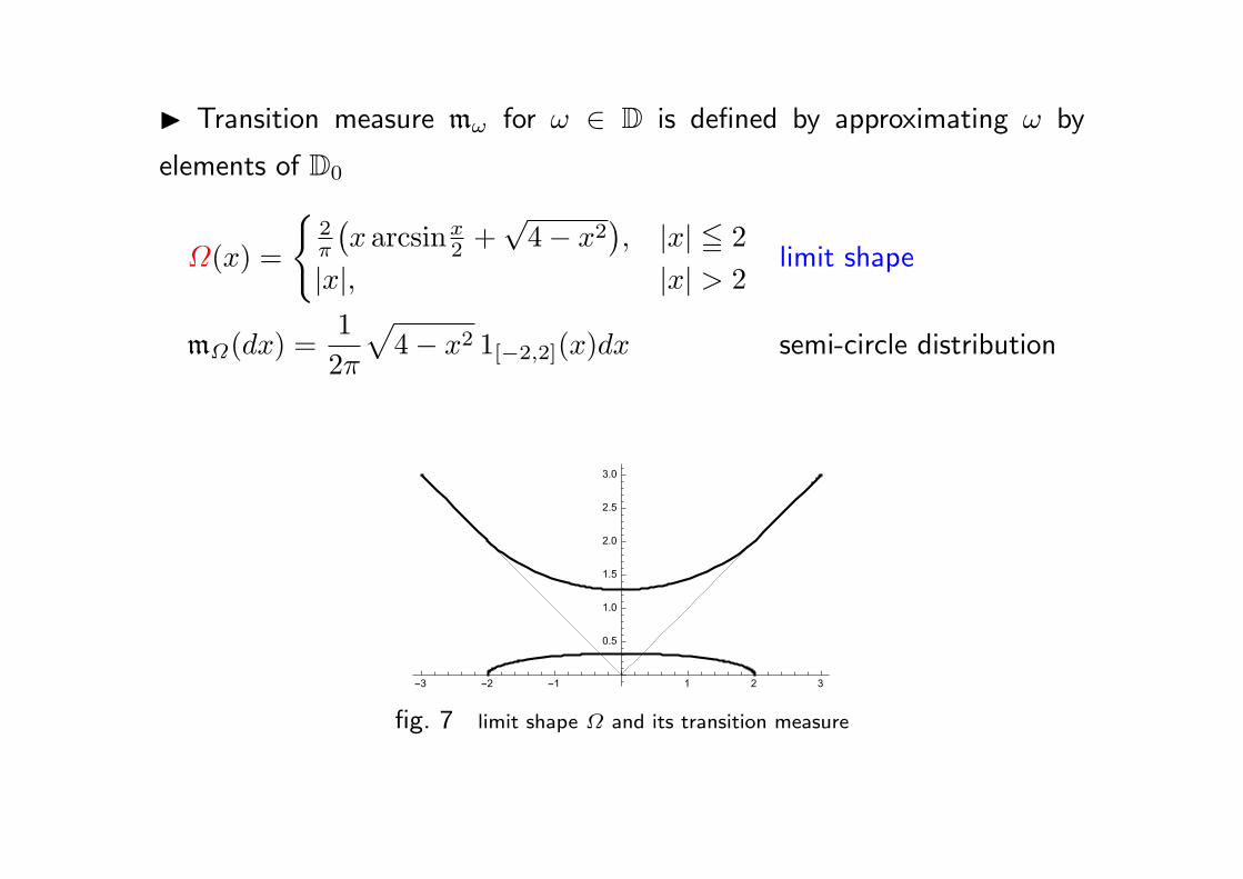
Transition measure mω for ω ∈ D is defined by approximating ω by

elements of D0

Ω(x) =

2π

(x arcsinx

2 +√4− x2

), |x| ≦ 2

|x|, |x| > 2limit shape

mΩ(dx) =1

2π

√4− x2 1[−2,2](x)dx semi-circle distribution

fig. 7 limit shape Ω and its transition measure

The following law of large numbers holds

(static scaling limit for the Plancherel measure)

Theorem (Vershik-Kerov, Logan-Shepp 1977)

M(n)Pl

(λ ∈ Yn

∣∣∣ supx∈R|λ

√n(x)−Ω(x)| ≧ ϵ

)= P

(∥Z

√n

n −Ω∥sup ≧ ϵ)

−−−−→n→∞

0 (∀ϵ > 0)

Namely, distribution of Z√n

n converges to δΩ as n→∞.

Strong law of large numbers also holds by considering the Plancherel measure

on the path space of the Young graph.

§3.6 Interface evolution

Dynamic scaling limit

s: microscopic time, t: macroscopic time s = tn

– spectral gap of transition matrix of Res-Ind chain is 2/n (§3.3 Lemma)

Given any initial macroscopic profile ω0 ∈ D s.t.

∫R(ω0(x)− |x|)dx = 2,

Take a sequence λ(n)n∈N s.t. λ(n) ∈ Yn, λ(n)√n → ω0 in D i.e.

limn→∞

∥∥λ(n)√n − ω0

∥∥sup

= 0.

Continuous time Res-Ind chain X(n)s with initial distribution on Yn:

P(X(n)0 = · ) = δλ(n)

Xtn(n)

√n −−−−→

n→∞? (deterministic macroscopic profile depending on t)

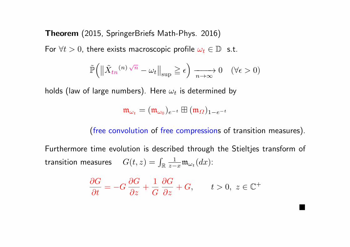
Theorem (2015, SpringerBriefs Math-Phys. 2016)

For ∀t > 0, there exists macroscopic profile ωt ∈ D s.t.

P(∥∥Xtn

(n)√n − ωt

∥∥sup

≧ ϵ)−−−−→n→∞

0 (∀ϵ > 0)

holds (law of large numbers). Here ωt is determined by

mωt= (mω0

)e−t ⊞ (mΩ)1−e−t

(free convolution of free compressions of transition measures).

Furthermore time evolution is described through the Stieltjes transform of

transition measures G(t, z) =∫R

1z−xmωt(dx):

∂G

∂t= −G ∂G

∂z+

1

G

∂G

∂z+G, t > 0, z ∈ C+

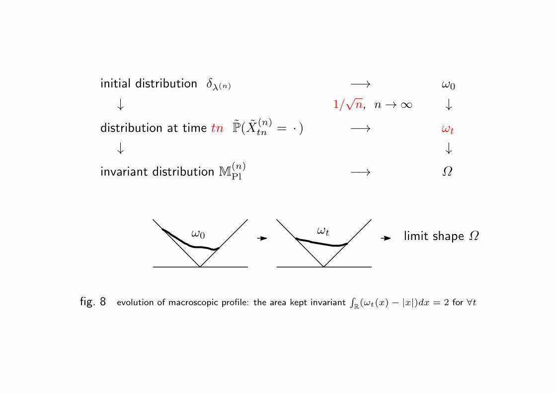
initial distribution δλ(n) −→ ω0

↓ 1/√n, n → ∞ ↓

distribution at time tn P(X(n)tn = · ) −→ ωt

↓ ↓

invariant distribution M(n)Pl −→ Ω

limit shape Ωω0ωt

fig. 8 evolution of macroscopic profile: the area kept invariant∫R(ωt(x) − |x|)dx = 2 for ∀t

Reference for §3

A. Hora: The Limit Shape Problem for Ensembles of Young Diagrams,

Springer Briefs in Mathematical Physics 17, Springer, 2016

END