Martin–Luther–Universitat

Halle–Wittenberg

Institut fur Mathematik

Festschrift zum 75. Geburtstag

von Prof. Dr. Alfred Gopfert

Andreas Lohne, Thomas Riedrich andChristiane Tammer

Report No. 07 (2009)

Editors:Professors of the Institute for Mathematics, Martin-Luther-University Halle-Wittenberg.

Electronic version: see http://www2.mathematik.uni-halle.de/institut/reports/

Festschrift zum 75. Geburtstag

von Prof. Dr. Alfred Gopfert

Andreas Lohne, Thomas Riedrich and

Christiane Tammer

Report No. 07 (2009)

Andreas LohneChristiane TammerMartin-Luther-Universitat Halle-WittenbergNaturwissenschaftliche Fakultat IIIInstitut fur MathematikTheodor-Lieser-Str. 5D-06120 Halle/Saale, GermanyEmail: andreas.loehne@mathematik.uni-halle.deEmail: christiane.tammer@mathematik.uni-halle.de

Thomas RiedrichTechnische Universitat DresdenFachrichtung MathematikD-01062 Dresden

Festschrift zum 75. Geburtstag von Prof. Dr. Alfred Göpfert

Es ist eine große Freude für uns, diese Beiträge unserem Lehrer, Mentor, Kollegen undFreund Alfred Göpfert anlässlich seines 75. Geburtstages zu widmen.

Prof. Dr. habil. Alfred Göpfert begann seine wissenschaftliche Laufbahn in den sechzigerJahren als Doktorand in der Arbeitsgruppe von Prof. Herbert Beckert an der UniversitätLeipzig. Hier beschäftigte er sich mit Problemstellungen aus dem Gebiet der partiellenDifferentialgleichungen, insbesondere mit approximativen Methoden bei der Behandlungvon Rand- und Eigenwertproblemen. Gleichzeitig entwickelte er ein großes Interesse anFragestellungen der Konvexen Analysis und der Optimierungstheorie. Im Jahr 1974 wurdeAlfred Göpfert Professor für Mathematik an der Technischen Hochschule Leuna-Merseburg.Hier baute er eine Forschungsgruppe auf, in der international viel beachtete Resultate aufden Gebieten der Optimierungstheorie in allgemeinen Räumen und der Funktionalanalysisentwickelt wurden. Professor Göpfert leitete diese Arbeitsgruppe sehr erfolgreich, betreu-te und förderte eine große Anzahl von Diplomarbeiten, Promotionen und Habilitationen.Von 1992 bis 1999 war Alfred Göpfert als Professor für Konvexe Analysis und Optimie-rung an der Martin-Luther-Universität Halle-Wittenberg tätig, bevor er 1999 emeritiertwurde, aber keineswegs in den Ruhestand ging. Von seinem breiten und umfassenden Wis-sen, seiner Ausstrahlung und seinen Anregungen profitierten Studenten und Kollegen derUniversitäten in Leipzig, Halle und der Technischen Hochschule Merseburg.

Die Resultate seiner Forschungsarbeiten stellte Alfred Göpfert auf vielen internationalenKonferenzen und in Veröffentlichungen in anerkannten Fachzeitschriften sowie in Büchernvor. Damit gab er Anstöße für neue Forschungsrichtungen, insbesondere auf den Gebietender Optimierung in allgemeinen Räumen und der funktionalanalytischen Grundlagen derOptimierung. Durch sein Buch Mathematische Optimierung in allgemeinen Vektorräumen(1973) erhielten viele Wissenschaftler Impulse für ihre Forschungsarbeit. Das Lehrbuch zurFunktionalanalysis (gemeinsam mit Thomas Riedrich) half Studenten und Wissenschaft-lern, einen Einstieg in dieses Gebiet zu finden. Ebenso stellen das gemeinsam mit ReinhardNehse veröffentlichte Buch Vektoroptimierung Theorie, Verfahren und Anwendungen (1990)und das Lexikon der Optimierung wichtige Beiträge zur Forschung auf dem Gebiet der Op-timierung dar. Im Jahr 2003 erschien die von Alfred Göpfert und Koautoren verfassteMonographie Variational Methods in Partially Ordered Spaces beim Springer-Verlag undim März 2009 das Lehrbuch Angewandte Funktionalanalysis beim Verlag Vieweg+Teubner.

Wir schätzen Alfred Göpfert als ausgezeichneten akademischen Lehrer, der wesentlich zurEntwicklung der Optimierungstheorie am Institut für Mathematik der Martin-Luther-Universität Halle-Wittenberg beigetragen hat. Mit seinen Anregungen unterstützte unsProf. Göpfert in seiner stets hilfsbereiten Art sehr bei unserer wissenschaftlichen Arbeit.Die Kollegen, die die Freude haben, mit ihm zusammenarbeiten zu können, profitieren vonseiner Fähigkeit, interessante Beziehungen zwischen unterschiedlichen Gebieten der Mathe-matik herzustellen. Für das Verfassen wichtiger Arbeiten mit einer außerordentlich großen

Anzahl von Koautoren waren die besondere Genauigkeit im Detail und die Fähigkeit vonAlfred Göpfert, wesentliche Zusammenhänge zu erkennen, prägend. Die Diskussionen mitihm wecken immer wieder Neugier auf interessante mathematische Fragestellungen.

Seine Tätigkeit als Wissenschaftler war immer verbunden mit einem Engagement in akade-mischen Gremien, Kommissionen und Verbänden. So hat er, um nur ein Beispiel zu nennen,als Vorsitzender des Landesverbandes Sachsen-Anhalt des Deutschen Hochschulverbandesgroßen Einfluss auf die Hochschulpolitik genommen.

Wir, seine Schüler und Kollegen, sind ihm für seine Anregungen, seine Unterstützung, Hilfeund Herzlichkeit sehr dankbar.

Christiane Tammer, Thomas Riedrich und Andreas Löhne

Inhaltsverzeichnis

On the Solution of Marginal-Sum Equations

Siegfried Dietze, Thomas Riedrich, Klaus D. Schmidt 1

Lagrange Duality in Vector Optimization – An Approach Based on Self-infimal Sets

Andreas Löhne, Christiane Tammer 17

Skalarisierungsfunktionale und deren Anwendungen

Christiane Tammer 35

On the Solution ofMarginal–Sum Equations

By Siegfried Dietze, Thomas Riedrich and Klaus D. Schmidt

Fachrichtung MathematikTechnische Universitat Dresden

Abstract

In motor car insurance, the risks of a portfolio usually are grouped accordingto the realizations of two (or more) risk characteristics and it is assumed that,for every group, the expected average claim amount can be represented as aproduct of parameters representing the realizations of the risk characteristics.This model leads, in a natural way, to the problem of marginal–sum estimationand hence to the problem of solving marginal–sum equations. Under theassumption that at least one observation is available in every group, we showthat a solution of the marginal–sum equations exists, that it is radially unique,and that it can be obtained by iteration with an arbitrary initial value.

1 Introduction

In motor car insurance, the risks of a portfolio usually are grouped according to therealizations of two or more risk characteristics.

In the case of two risk characteristics, it is assumed that, for every group, the claimnumber Ni,k and the aggregate claim amount Si,k are related by the model equations

E

[Si,k

Ni,k

]= µαi βk

where µ is a scale parameter and the parameters αi and βk with i ∈ 1, . . . , I andk ∈ 1, . . . , K refer to the realizations of the risk characteristics.

Since expectations of quotients are difficult to handle in general, it is convenient toreplace expectations of quotients by quotients of expectations and hence to replacethe previous model equations by the equations

µαi βk E[Ni,k] = E[Si,k]

1

Summation yields

K∑l=1

µαi βl E[Ni,l] =K∑

l=1

E[Si,l] andI∑

j=1

µαj βk E[Nj,k] =I∑

j=1

E[Sj,k]

with i ∈ 1, . . . , I and k ∈ 1, . . . , K. Replacing all parameters and expectationsin these equations by random variables, we obtain the marginal–sum equations

K∑l=1

µ αi βl Ni,l =K∑

l=1

Si,l andI∑

j=1

µ αj βk Nj,k =I∑

j=1

Sj,k

with i ∈ 1, . . . , I and k ∈ 1, . . . , K. We say that random variables µ, α1, . . . , αI ,

β1, . . . , βK are marginal–sum estimators of the parameters µ, α1, . . . , αI , β1, . . . , βK

if they solve the marginal–sum equations.

Although it seems to be unknown until now whether or not marginal–sum estimatorsexist, their existence is usually taken as granted and iteration methods are used todetermine approximations. The present paper is intended as a first but essentialstep to close this gap.

In spite of the probabilistic model justifying marginal–sum estimation, the problemof the existence of marginal–sum estimators is essentially non–probabilistic. Wethus propose a deterministic approach to the solution of the marginal equations(Section 2) and relate this problem to a fixed point problem (Section 3). Under theassumption that all claim numbers are strictly positive and that the right hand sideof each of the marginal–sum equations is strictly positive as well, we show that themarginal–sum equations have a solution (Section 4) which is radially unique (in asense to be made precise) and can be obtained by iteration (Section 5). We concludewith some remarks on impossible and possible extensions of our results (Section 6)and on marginal–sum estimation in loss reserving (Section 7).

2 The Marginal–Sum Equations

Throughout this paper, we consider two matrices N,S ∈ RI+ × RK

+ having theproperty that every row vector and every column vector of each of N and S has atleast one coordinate which is nonzero; this means that e′iN1,1′Nek, e

′iS1,1′Sek > 0

holds for all i ∈ 1, . . . , I and k ∈ 1, . . . , K (where ei ∈ RI and ek ∈ RK are unitvectors and 1 is a vector of suitable dimension with all coordinates being equal to 1).The assumption on the matrix N will be strengthened in Sections 4 and 5 below.

We are interested in solutions (µ,α,β) ∈ (0,∞)×(0,∞)I×(0,∞)K of the marginal–sum equations

K∑l=1

µαi βl Ni,l =K∑

l=1

Si,l andI∑

j=1

µαj βk Nj,k =I∑

j=1

Sj,k

with i ∈ 1, . . . , I and k ∈ 1, . . . , K.

2

The marginal–sum equations have either no solution or infinitely many solutions:Indeed, if (µ,α,β) is a solution, then (1, µα,β) and (1,α, µβ) are solutions as well;more generally, if (µ,α,β) is a solution and if c, d 6= 0, then ((cd)−1µ, cα, dβ) is asolution as well.

The parameter µ is obviously of minor interest: Indeed, if (µ,α,β) is a solution ofthe marginal equations, then

µ =

∑Ij=1

∑Kl=1 Sj,l∑I

j=1

∑Kl=1 αj Nj,l βl

This shows that the parameter µ is nothing else than a scaling parameter whichpermits any scaling of the parameters α and β by a strictly positive factor. Forexample, the parameters α and β may be scaled by the requirement that either

1′α = 1 and 1′β = 1

or

maxj∈1,...,I

αj = 1 and maxl∈1,...,K

βl = 1

Scaling the parameters α and β may be of substantial interest in actuarial practice.

Because of the preceding discussion, we now simplify the terminology by saying thatthe pair (α,β) ∈ (0,∞)I × (0,∞)K is a solution of the marginal–sum equations ifthere exists some µ ∈ (0,∞) such that the triplet (µ,α,β) is a solution of themarginal–sum equations; in that case, we have

µ =1′S1

α′Nβ

We also say that the marginal–sum equations have a radially unique solution if theyhave a solution (α∗,β∗) and if every solution (α,β) satisfies

α = cα∗ and β = dβ∗

for some c, d ∈ (0,∞).

Under the rather restrictive assumption that all coordinates of the matrix N areidentical, it is easily seen that the marginal–sum equation have a radially uniquesolution and that the solutions can be given in closed form:

2.1 Example. Assume that Ni,k = ν holds for some ν ∈ (0,∞) and for alli ∈ 1, . . . , I and all k ∈ 1, . . . , K. Then the marginal–sum equations can bewritten as

µν α =S1

1′βand µν β =

S′1

1′α

3

Thus, letting

α∗ :=S1

1′S1and β∗ :=

S′1

1′S1

we see that (α∗,β∗) is a solution of the marginal equations (with µ∗ = 1′S1/ν)which satisfies

1′α∗ = 1 and 1′β∗ = 1

Moreover, every solution (α,β) of the marginal equations satisfies

α = cα∗ and β = dβ∗

for some c, d ∈ (0,∞) such that the marginal–sum equations have a radially uniquesolution.

In the general case, however, the existence and the radial uniqueness of solution ofthe marginal–sum equations are far from being evident.

3 Equivalent Fixed Point Problems

The marginal–sum equations may be expressed in terms of nonlinear maps:

Define first G : (0,∞)I → (0,∞)K and H : (0,∞)K → (0,∞)I coordinatewise byletting

Gk(α) :=1′Sek

α′Nek

and Hi(β) :=e′iS1

e′iNβ

Then a pair (α,β) ∈ (0,∞)I × (0,∞)K is a solution of the marginal–sum equationsif and only if there exists some µ ∈ (0,∞) such that

µα = H(β) and µβ = G(α)

In that case, we have

µ =1′S1

α′Nβ

The following lemma is obvious:

3.1 Lemma. Each of the maps G and H is(i) homogeneous of degree −1,(ii) monotone decreasing , and(iii) continuous.

4

Here and in the sequel, inequalities between vectors, order intervals, and monotonic-ity of maps refer to the coordinatewise order relation on the Euclidean space.

Define now Φ : (0,∞)I → (0,∞)I and Ψ : (0,∞)K → (0,∞)K by letting

Φ := H G and Ψ := G H

The following lemma records some basic properties of Φ and Ψ which are evidentfrom the definitions and Lemma 3.1:

3.2 Lemma. Each of the maps Φ and Ψ is(i) homogeneous of degree 1,(ii) monotone increasing , and(iii) continuous.Moreover , the maps Φ and Ψ satisfy G Φ = Ψ G and Φ H = H Ψ.

The following result relates the solutions of the marginal–equations and the fixedpoints of Φ and Ψ to each other:

3.3 Theorem.(1) If (α,β) is a solution of the marginal equations , then α is a fixed point of Φ

and β is a fixed point of Ψ.(2) If α is a fixed point of Φ, then G(α) is a fixed point of Ψ and (α,G(α)) is a

solution of the marginal equations.(3) If β is a fixed point of Ψ, then H(β) is a fixed point of Φ and (H(β),β) is a

solution of the marginal equations.

Proof. Assume first that (α,β) is a solution of the marginal equations and define

µ :=1′S1

α′Nβ

Lemma 3.1 yields

µα = H(β)

= H(µ−1 G(α))

= µH(G(α))

= µΦ(α)

and hence

α = Φ(α)

By symmetry, we obtain

β = Ψ(β)

This proves (1).

5

Assume now that α is a fixed point of Φ. Then we have

Φ(α) = α

and Lemma 3.2 yields

Ψ(G(α)) = G(Φ(α))

= G(α)

which means that G(α) is a fixed point of Ψ. Furthermore, letting

β := G(α)

we obtain

α = Φ(α)

= H(G(α))

= H(β)

which means that (α,β) is a solution of the marginal–sum equations (with µ = 1).This proves (2), and (3) follows by symmetry. 2

We say that a map Γ : (0,∞)d → (0,∞)d has a radially unique fixed point if Γ hasa fixed point z∗ and if every fixed point z of Γ satisfies

z = c z∗

for some c ∈ (0,∞).

3.4 Theorem. The following are equivalent :(a) The marginal–sum equations have a radially unique solution.(b) The map Φ has a radially unique fixed point.(c) The map Ψ has a radially unique fixed point.

Proof. Assume first that the marginal–sum equations have a radially uniquesolution (α∗,β∗) and consider any fixed point α of Φ. By Theorem 3.3, (α,G(α))is a solution of the marginal–sum equations and it now follows that there existssome c ∈ (0,∞) such that

α = cα∗

Therefore, (a) implies (b), and it follows by symmetry that (a) implies (c).Assume now that Φ has a radially unique fixed point α∗ and consider any fixedpoint β of Ψ. By Theorem 3.3,

β∗ := G(α∗)

6

is a fixed point of Ψ and H(β) is a fixed point of Φ. It now follows that there existssome c ∈ (0,∞) such that

H(β) = cα∗

and we obtain

β = Ψ(β)

= G(H(β))

= G(cα∗)

= c−1 G(α∗)

= c−1 β∗

Therefore, (b) implies (c), and it follows by symmetry that (c) implies (b).Assume finally that Φ has a radially unique fixed point α∗ and consider any solution(α,β) of the marginal–sum equations. By Theorem 3.3, α is a fixed point of Φ andβ is a fixed point of Ψ. By what we have shown before, we know that also Ψ hasa radially unique fixed point β∗. It now follows that there exist some c, d ∈ (0,∞)such that

α = cα∗ and β = dβ∗

Therefore, (b) implies (a), and it follows by symmetry that (c) implies (a). 2

4 Existence of a Fixed Point of Φ

In the present section, we assume that all coordinates of N are strictly positive; thismeans that e′iNek > 0 holds for all i ∈ 1, . . . , I and k ∈ 1, . . . , K

Define G : RI+ \ 0 → (0,∞)K and H : RK

+ \ 0 → (0,∞)I coordinatewise byletting

Gk(α) :=1′Sek

α′Nek

and H i(β) :=e′iS1

e′iNβ

(where 0 is a vector of suitable dimension with all coordinates being equal to 0) anddefine Φ : RI

+ \ 0 → (0,∞)I and Ψ : RK+ \ 0 → (0,∞)K by letting

Φ := H G and Ψ := G H

Then Φ extends Φ, and Ψ extends Ψ. By symmetry, it is sufficient to study theproperties of Φ.

We can now prove the existence of a fixed point of Φ:

4.1 Theorem. The map Φ has a fixed point.

7

Proof. Let

∆I := α ∈ RI+ | 1′α = 1

and define Φ : ∆I → ∆I by letting

Φ(α) :=1

1 + 1′Φ(α)

(α + Φ(α)

)Then the set ∆I is nonempty, convex and compact, and the map Φ is continuoussince Φ is continuous. It now follows from Brouwer’s Fixed Point Theorem that Φhas a fixed point; see e. g. Granas and Dugundji [2003; Theorems 7.1 and 7.2].

Assume now that α is a fixed point of Φ. Then we have Φ(α) = α and hence

Φ(α) = λα

with λ := 1′Φ(α). For all i ∈ 1, . . . , I, we thus have Φi(α) = λαi and hence

K∑l=1

Si,l = λαi

K∑l=1

Ni,l

∑Ij=1 Sj,l∑I

j=1 αj Nj,l

Summation yields∑I

i=1

∑Kl=1 Si,l = λ

∑Kl=1

∑Ij=1 Sj,l and hence λ = 1. We thus

obtain

Φ(α) = α

which means that α is also a fixed point of Φ. Since α = Φ(α) ∈ (0,∞)I , we seethat α is even a fixed point of Φ. 2

It now follows from Theorems 4.1 and 3.3 that the marginal–sum equations have asolution whenever all entries of the matrix N are strictly positive.

5 Convergence of Iterates and

Radial Uniqueness of the Fixed Points of Φ

As in the previous section, we assume that all coordinates of N are strictly positiveand we consider only the map Φ.

5.1 Lemma. Every coordinate of Φ is partially differentiable. Moreover , for everyinterval [u, z] ⊆ (0,∞)I , there exists some γ ∈ (0,∞) such that

∂Φi

∂tj(t) ≥ γ

holds for all i, j ∈ 1, . . . , I and t ∈ [u, z].

8

Proof. For i, j ∈ 1, . . . , I, define Ui, Zi,j : (0,∞)I → (0,∞) by letting

Ui(t) :=

K∑l=1

Si,l(K∑

l=1

Ni,l

∑Ih=1 Sh,l∑I

h=1 thNh,l

)2

and

Zi,j(t) :=K∑

l=1

Ni,l Nj,l

∑Ih=1 Sh,l(∑I

h=1 thNh,l

)2

Then Ui is monotone increasing and Zi,j is monotone decreasing, and we obtain

∂Φi

∂tj(t) = Ui(t)Zi,j(t)

≥ Ui(u)Zi,j(z)

for all t ∈ [u, z]. Letting γ := mini,j∈1,...,I Ui(u)Zi,j(z) yields the assertion. 2

By Theorem 4.1, the map Φ has a fixed point. Using Lemma 5.1, we can now provethe following result on the convergence of the iterates under Φ of an arbitrary vectorin the domain of Φ:

5.2 Theorem. Let α be a fixed point of Φ. Then, for every x ∈ (0,∞)I , thereexists some ξ ∈ (0,∞) such that the sequence Φn(x)n∈N0 converges to ξα.

Proof. For all n ∈ N0, define

x(n) := Φn(x)

as well as

u(n) := λ(n)α and z(n) := µ(n)α

with

λ(n) := mini∈1,...,I

x(n)i

αi

and µ(n) := maxi∈1,...,I

x(n)i

αi

Then we have

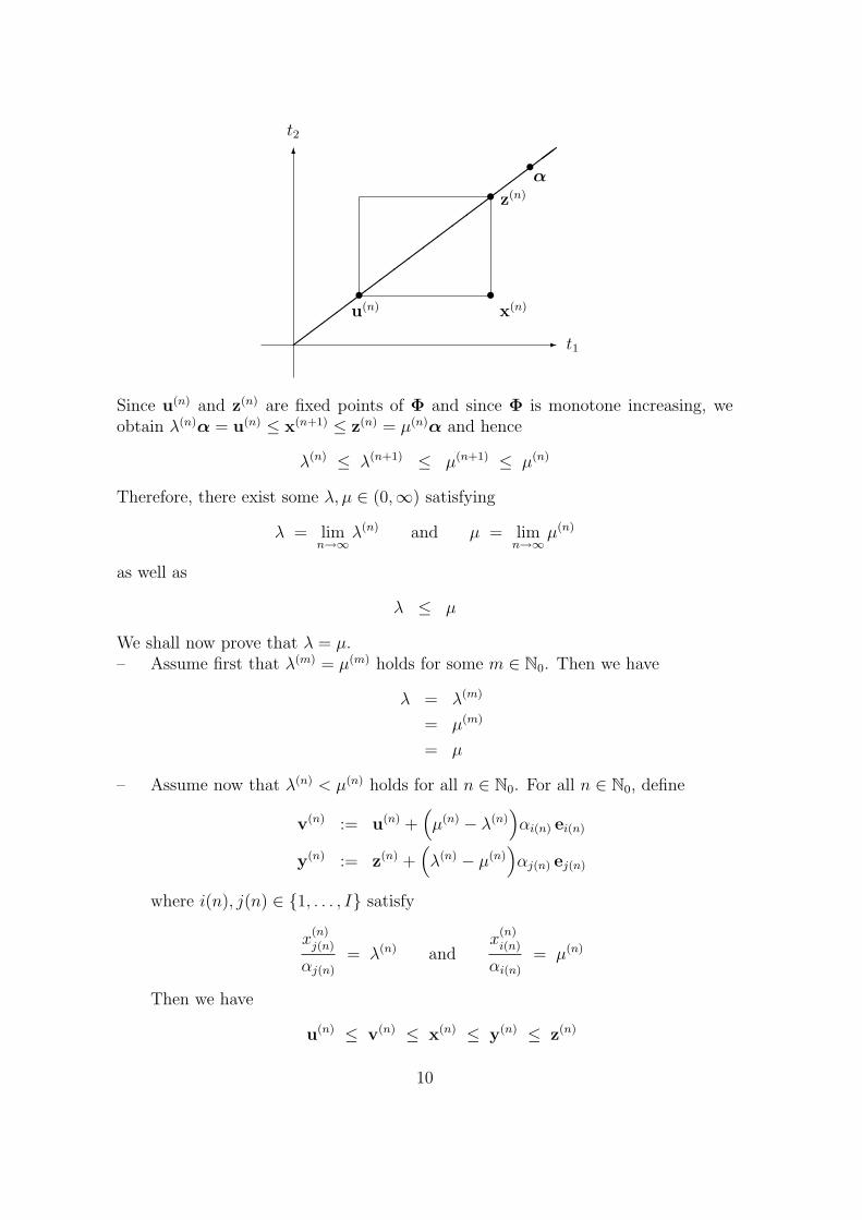
u(n) ≤ x(n) ≤ z(n)

This construction is illustrated by the following picture:

9

- t1

6

t2

•u(n)

•x(n)

• z(n)

•α

Since u(n) and z(n) are fixed points of Φ and since Φ is monotone increasing, weobtain λ(n)α = u(n) ≤ x(n+1) ≤ z(n) = µ(n)α and hence

λ(n) ≤ λ(n+1) ≤ µ(n+1) ≤ µ(n)

Therefore, there exist some λ, µ ∈ (0,∞) satisfying

λ = limn→∞

λ(n) and µ = limn→∞

µ(n)

as well as

λ ≤ µ

We shall now prove that λ = µ.– Assume first that λ(m) = µ(m) holds for some m ∈ N0. Then we have

λ = λ(m)

= µ(m)

= µ

– Assume now that λ(n) < µ(n) holds for all n ∈ N0. For all n ∈ N0, define

v(n) := u(n) +(µ(n) − λ(n)

)αi(n) ei(n)

y(n) := z(n) +(λ(n) − µ(n)

)αj(n) ej(n)

where i(n), j(n) ∈ 1, . . . , I satisfy

x(n)j(n)

αj(n)

= λ(n) andx

(n)i(n)

αi(n)

= µ(n)

Then we have

u(n) ≤ v(n) ≤ x(n) ≤ y(n) ≤ z(n)

10

Define

γ := mini,j∈1,...,I

inft∈[u(0),z(0)]

∂Φi

∂tj(t)

By Lemma 5.1, we have γ ∈ (0,∞).Since z(n) is a fixed point of Φ and since Φ is monotone increasing, we obtain

z(n) − x(n+1) = Φ(z(n))−Φ(x(n))

≥ Φ(z(n))−Φ(y(n))

Now, for every i ∈ 1, . . . , I, the mean value theorem yields the existence ofsome t(n,i) ∈ [y(n), z(n)] ⊆ [u(0), z(0)] such that

z(n)i − x

(n+1)i ≥ Φi(z

(n))− Φi(y(n))

=

(∂Φi

∂tj(n)

(t(n,i))

)(z

(n)j(n) − y

(n)j(n)

)=

(∂Φi

∂tj(n)

(t(n,i))

)(µ(n) − λ(n)

)αj(n)

≥ γ(µ(n) − λ(n)

)min

j∈1,...,Iαj

Repeating the argument yields

x(n+1)i − u(n)

i ≥ γ(µ(n) − λ(n)

)min

j∈1,...,Iαj

for all i ∈ 1, . . . , I. We thus obtain

z(n+1) = µ(n+1) α

=x

(n+1)i(n+1)

αi(n+1)

α

≤ 1

αi(n+1)

(z

(n)i(n+1) − γ

(µ(n) − λ(n)

)min

j∈1,...,Iαj

)α

≤(µ(n) − γ

(µ(n) − λ(n)

)minj∈1,...,I αj

maxj∈1,...,I αj

)α

as well as

u(n+1) ≥(λ(n) + γ

(µ(n) − λ(n)

)minj∈1,...,I αj

maxj∈1,...,I αj

)α

Combining these two inequalities, we obtain(µ(n+1) − λ(n+1)

)α = z(n+1) − u(n+1)

≤(µ(n) − λ(n)

)(1− 2 γ

minj∈1,...,I αj

maxj∈1,...,I αj

)α

11

and hence

0 ≤ µ(n+1) − λ(n+1) ≤(µ(n) − λ(n)

)(1− 2 γ

minj∈1,...,I αj

maxj∈1,...,I αj

)for all n ∈ N0. Since γ ∈ (0,∞), we have

1− 2 γminj∈1,...,I αj

maxj∈1,...,I αj

< 1

and it follows that

λ = limn→∞

λ(n)

= limn→∞

µ(n)

= µ

Therefore, we have in both cases λ = µ and this yields

limn→∞

u(n) = λα

= µα

= limn→∞

z(n)

Since u(n) ≤ x(n) ≤ z(n), it follows that the sequence x(n)n∈N0 converges to thefixed point λα = µα of Φ. 2

As an immediate consequence of the previous result, we obtain the radial uniquenessof the fixed points of Φ:

5.3 Theorem. The map Φ has a radially unique fixed point.

It now follows from Theorems 5.3 and 3.4 that the marginal–sum equations havea radially unique solution whenever all coordinates of the matrix N are strictlypositive.

The proof of Theorem 5.2 uses a method presented in Morishima [1964; Appendix,Section 2] for the solution of a nonlinear eigenvalue problem. An alternative proofcould be given by using Krasnoselskii [1964; Theorems 5.5 and 5.6]. The radialuniqueness of fixed points, which in present paper is obtained as a consequence ofTheorem 5.2, could also be obtained from results in Morishima [1964; Appendix,Section 2].

6 Possible Extensions

Since the data represented by the matrices N and S are realizations of randommatrices, it may happen that at least one class (i, k) ∈ 1, . . . , I × 1, . . . , Kcontains no observations such that the number of claims Ni,k and hence also theaggregate claim size Si,k is equal to zero.

12

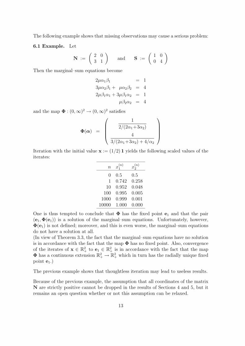
The following example shows that missing observations may cause a serious problem:

6.1 Example. Let

N :=

(2 03 1

)and S :=

(1 00 4

)Then the marginal–sum equations become

2µα1β1 = 1

3µα2β1 + µα2β2 = 4

2µβ1α1 + 3µβ1α2 = 1

µβ2α2 = 4

and the map Φ : (0,∞)2 → (0,∞)2 satisfies

Φ(α) =

1

2/(2α1+3α2)

4

3/(2α1+3α2) + 4/α2

Iteration with the initial value x := (1/2) 1 yields the following scaled values of theiterates:

n x(n)1 x

(n)2

0 0.5 0.51 0.742 0.258

10 0.952 0.048100 0.995 0.005

1000 0.999 0.00110000 1.000 0.000

One is thus tempted to conclude that Φ has the fixed point e1 and that the pair(e1,Φ(e1)) is a solution of the marginal–sum equations. Unfortunately, however,Φ(e1) is not defined; moreover, and this is even worse, the marginal–sum equationsdo not have a solution at all.(In view of Theorem 3.3, the fact that the marginal–sum equations have no solutionis in accordance with the fact that the map Φ has no fixed point. Also, convergenceof the iterates of x ∈ R2

+ to e1 ∈ R2+ is in accordance with the fact that the map

Φ has a continuous extension R2+ → R2

+ which in turn has the radially unique fixedpoint e1.)

The previous example shows that thoughtless iteration may lead to useless results.

Because of the previous example, the assumption that all coordinates of the matrixN are strictly positive cannot be dropped in the results of Sections 4 and 5, but itremains an open question whether or not this assumption can be relaxed.

13

The marginal–sum equations may also be extended to more than two risk charac-teristics. For example, in the case of three risk characteristics the marginal–sumequations become

K∑l=1

M∑n=1

µαi βl γnNi,l,n =K∑

l=1

M∑n=1

Si,l,n

I∑j=1

M∑n=1

µαj βk γnNj,k,n =I∑

j=1

M∑n=1

Sj,k,n

I∑j=1

K∑l=1

µαj βl γmNj,l,m =I∑

j=1

K∑l=1

Sj,l,m

with i ∈ 1, . . . , I, k ∈ 1, . . . , K andm ∈ 1, . . . ,M. In the case of three or morerisk characteristics, it is an open question whether the marginal–sum equations havea solution, whether the solution is radially unique, and whether it can be obtainedby iteration.

7 Remark

Marginal–sum equations also occur in loss reserving based on run–off triangles. Inthat case, the data are represented in a triangle instead of a rectangle and it iswell–known that the marginal–sum equations have a unique solution which justifiesthe chain–ladder method; see Mack [1991, 2003], Schmidt and Wunsche [1998], andRadtke and Schmidt [2004].

Acknowledgement

The authors would like to thank Mathias Zocher for a discussion of marginal–sumestimation.

References

Granas, A., and Dugundji, J. [2003]: Fixed Point Theory. Berlin – Heidelberg – NewYork: Springer.

Krasnoselskii, M. A. [1964]: Positive Solutions of Operator Equations. (Translatedfrom the Russian.) Groningen: Noordhoff.

Mack, T. [1991]: A simple parametric model for rating automobile insurance or esti-mating IBNR claims reserves. ASTIN Bull. 21, 93–109.

Mack, T. [2002]: Schadenversicherungsmathematik. 2. Auflage. Karlsruhe: VerlagVersicherungswirtschaft.

14

Morishima, M. [1964]: Equilibrium, Stability and Growth: A Multisectoral Analysis.Oxford: Clarendon Press.Radtke, M., and Schmidt, K. D. [2004]: Handbuch zur Schadenreservierung. Karls-ruhe: Verlag Versicherungswirtschaft.Schmidt, K. D., and Wunsche, A. [1998]: Chain–ladder, marginal–sum and maxi-mum–likelihood estimation. Blatter DGVM 23, 289–307.

Siegfried DietzeThomas RiedrichKlaus D. SchmidtFachrichtung MathematikTechnische Universitat DresdenD–01062 Dresden

e–mail: klaus.d.schmidt@tu-dresden.de

April 17, 2009

15

16

Lagrange duality in vector optimization - An approachbased on self-infimal sets

Andreas Lohne Christiane Tammer

Dedicated to Prof. Dr. Alfred Gopfert on the occasion of his 75th birthday

AbstractIn this article a new type of vectorial Lagrange duality is investigated. As the ob-jective space of a given vector optimization problem is embedded into a larger space,in fact, the space of self-infimal subsets of the original vector space, it is possible towork with infimum and supremum in the sense of the greatest lower and least upperbound, respectively. As a consequence, a weak and a strong vectorial Langrange du-ality theorem can be formulated very similar to the well-known scalar counterparts.

1 Introduction

It is well known that a maximization problem (φ(λ) → max with supremal value d) canbe associated to a given minimization problem (f(x) → min with infimal value p) suchthat d ≤ p and that, under additional assumptions, both problems have the same optimalvalues. Duality theory has been developed for many problem classes and for very generalsettings. One of the first contributions to duality theory in general spaces is given in thebook [10] by A. Gopfert.

There are at least three reasons to look for useful dual problems: First, the dualproblem has (under appropriate assumptions) the same optimal value as the given “primal”optimization problem, but solving the dual problem could be done with other methodsof analysis or numerical mathematics. Secondly, an approximate solution of the givenminimization problem gives an estimation of the minimal value p from above, whereasan approximate solution of the dual problem is an estimation of p from below, so thatone gets intervals that contain p. Moreover, recalling the Lagrange method, saddle points,equilibrium points of two-person games, shadow prices in economics, perturbation methodsor dual variational principles, it becomes clear that optimal dual variables often have aspecial meaning for the given problem.

Of course, the advantages just listed require a skillfully chosen dual program. Never-theless, the mentioned points are motivation enough, to look for dual problems in vectoroptimization too. However, it is not easy to derive useful dual problems in vector opti-mization. In the book by A. Gopert and R. Nehse [11, Page 64] one can find the followingremark on vectorial duality:

17

”... Die praktische Nutzung ist aber gegenuber der Nutzung der Dualitat derskalaren Optimierung noch wenig ausgepragt. Fur die Aufgabenklassen der lin-earen Vektoroptimierung, der vektoriellen Standortprobleme, der vektoriellengeometrischen Optimierung gibt es anwendungsfahige Dualprobleme, und siesind nicht komplizierter als die gegebenen Probleme. ...”

This remark can be understood as a motivation to consider new approaches to vectorialduality theory.

As in the scalar duality theory, there are different types, such as conjugate duality,Langrange duality and others, for instance, axiomatic duality. Lagrange duality theory isan important standard tool in optimization. There are many approaches to a correspondingtheory for vector optimization problems, see e.g., the book by Gopfert et al. [12, Section3.7] as well as the books by Jahn [19, 21] and Luc [27]. See also [34, 5, 38, 6, 7, 18, 33, 35,28, 9, 13, 29, 37, 4] for a choice of further papers on vectorial duality. The basic idea ofLagrange duality is to assign to a given constrained optimization problem

(p) p := infx∈S

f(x)

a Lagrange function L : X × Λ → R with supλ L(x, λ) = f(x) for x ∈ S ⊆ X and toconsider the closely related pair of mutually dual unconstrained problems

infx

supλL(x, λ) and sup

λinfxL(x, λ).

The dual problem is usually defined as

(d) d := supλφ(λ),

where λ is called the dual variable and φ : Λ→ R, φ(λ) := infx L(x, λ) is called the dualobjective function.

This shows that the concepts of infimum and supremum play an important role inLagrange duality. The vectorial approaches in the literature are based on an appropriatereplacement for these concepts. On the one hand, it is important to have a relationship ofthe supremum/infimum to the solution concepts and on the other hand the properties ofthe infimum/supremum (to be a greatest lower / least upper bound) are important for theproofs. We want to speak about a (complete) lattice structure in the latter case becausea partially ordered set is called a complete lattice if every subset has and infimum and asupremum in the sense of a greatest lower / least upper bound.

One possibility to re-obtain the lattice structure in vector optimization is to scalarizethe Lagrange function and to use the usual infimum/supremum in the complete latticeR := R ∪ +∞ ∪ −∞. In the most papers mentioned above the direct usage of infu-mum/supremum is essentially avoided. In other papers the infimum/supremum is hidden,but was not pointed out; see, e.g., [37].

18

We intend to work even in vector optimization consequently with an appropriate latticestructure. For that reason the image space of the objective function of the vector opti-mization problem is embedded into a larger space, namely into a subset of the power setof the original image space. Our approach ensures both, the lattice structure of the imagespace and the possibility to describe solutions of the vectorial problem by the correspond-ing infimum/supremum. This approach was established by Lohne and Tammer [26], wherea conjugate duality theory has been developed. Solution concepts in this framework havebeen recently defined and investigated by Heyde and Lohne [17]. Earlier works, such as[14, 24, 25, 16], are related but the relationship to vector optimization was not yet pointetout. Hamel developed in [14] and several forthcoming papers a Set-valued Convex Anal-ysis, in particualar in [15] also a Langrage duality theory in this setting. His set-valuedapproach is closely related to the present one, which is adapted to vector optimization.However, his set-valued approach has the advantage that it can be formulated in a moregeneral framework.

Let us finally mention that Kuroiwa [22] started to consider Lagrange duality by anordering relation in the power set. He did not, however, focus on the lattice structure.

2 Problem Formulation

Throughout the paper let C ( Rq be a pointed (i.e., C ∩ −C = 0) closed convex conewith nonempty interior. By C we denote its polar cone, i.e., C := y∗ ∈ Rq| ∀y ∈ C :〈y∗, y〉 ≤ 0. The set of weakly minimal points of a subset A ⊆ Rq (with respect to C) isdefined by

wMinA := y ∈ A| (y − intC) ∩ A = ∅ ,

and the set of minimal points of A is defined by

MinA := y ∈ A| (y − C \ 0) ∩ A = ∅ .

Let F : Rn → Rq and S ⊆ Rn. We consider the following vector optimization problem:

(VOP) P := MinF (S) := Min⋃x∈S

F (x) .

A feasible point x ∈ S is called an efficient solution of (VOP) if F (x) ∈ MinF (S). Thiscan be equivalently expressed as

[x ∈ S, F (x) ≤C F (x)] =⇒ F (x) = F (x).

Weakly efficient solutions are defined analoguosly, but we will only consider efficient solu-tions in this paper. Nevertheless the theory essentially works with weakly minimal points,for instance, the next section is based on this concept.

19

3 Infimal sets and infimum

We recall in this section the concept of an infimal set (resp. supremal set), which is dueto Nieuwenhuis [30], was extended by Tanino [36], and slightly modified with respect tothe elements ±∞ by Lohne and Tammer [26]. Moreover we recall properties of the spaceof self-infimal sets, which was shown in [26] to be a complete lattice. As we will show inSection 4, this complete lattice is usefull for the theory of vector optimization.

The upper closure (with respect to C) of A ⊆ Rq is defined (see e.g. [9]) to be the set

Cl +A := y ∈ Rq| y+ intC ⊆ A+ intC .

It is an easy task to show that for every (not necessarily convex) set A ⊆ Rq it holds

Cl +A = cl (A+ intC) = cl (A+ C). (1)

If A 6= ∅ we have [30, Th. I-18]

wMin Cl +A = ∅ ⇐⇒ A+ intC = Rq ⇐⇒ Cl +A = Rq.

The definition of the upper closure can be extended for subsets of the space Rq:= Rq ∪

−∞∪+∞. It is possible but not necessary for the present article to introduce calculusrules in Rq

.For a subset A ⊆ Rq

we set

Cl +A :=

Rq if −∞ ∈ Ay ∈ Rq| y+ intC ⊆ A \ +∞+ intC otherwise.

Clearly, the upper closure of a subset of Rqis always a subset in Rq.

The infimal set of A ⊆ Rq(with respect to C) is defined by

Inf A :=

wMin Cl +A if ∅ 6= Cl +A 6= Rq

−∞ if Cl +A = Rq

+∞ if Cl +A = ∅.

We see that the infimal set of A with respect to C coincides essentially with the set ofweakly minimal elements of the set cl (A+ C).

By our conventions, Inf A is always a nonempty set. Clearly, if −∞ belongs to A, wehave Inf A = −∞, in particular, Inf −∞ = −∞. Furthermore, it holds Inf ∅ =Inf +∞ = +∞ and Cl +A = Cl +(A ∪ +∞) and hence Inf A = Inf(A ∪ +∞) forall A ⊆ Rq

.The following assertions were proved by Nieuwenhuis [30] and, in an extended form, by

Tanino [36].

Proposition 3.1 For A,B ⊆ Rq with ∅ 6= Cl +A 6= Rq and ∅ 6= Cl +B 6= Rq it holds

(i) Inf A = y ∈ Rq| y 6∈ A+ intC, y+ intC ⊆ A+ intC,

20

(ii) A+ intC = B + intC ⇐⇒ Inf A = Inf B,

(iii) A+ intC = Inf A+ intC,

(iv) Cl +A = Inf A ∪ (Inf A+ intC),

(v) Inf A, (Inf A− intC) and (Inf A+ intC) are disjoint,

(vi) Inf A ∪ (Inf A− intC) ∪ (Inf A+ intC) = Rq.

(vii) Inf(Inf A+ Inf B) = Inf(A+B),

(viii) α Inf A = Inf(αA) for α > 0.

For A ⊆ Rqit holds

(ix) Inf Inf A = Inf A, Cl +Cl +A = Cl +A, Inf Cl +A = Inf A, Cl + Inf A = Cl +A,

Proposition 3.2 Let Ai ∈ Rqfor i ∈ I, where I is an arbitrary index set. Then it holds

(i) Cl +

⋃i∈I

Ai = Cl +

⋃i∈I

Cl +Ai,

(ii) Inf⋃i∈I

Ai = Inf⋃i∈I

Inf Ai.

Proof. (i) As Cl + +∞ = ∅ and Cl +A = Cl +(A \ +∞) we can assume that +∞ 6∈⋃i∈I Ai. We also assume −∞ 6∈

⋃i∈I Ai, because the statement is otherwise obvious.

So we have

Cl +

⋃i∈I

Ai = cl

(⋃i∈I

Ai + C

)= cl

(⋃i∈I

cl (Ai + C)

)+ C = Cl +

⋃i∈I

Cl +Ai.

(ii) Follows from (i) and Proposition 3.1 (ix).

One can define analogously, using the set wMaxA := −wMin(−A) of weakly maximalelements of A ⊆ Rq, the lower closure Cl −A and the set SupA of supremal elements ofA ⊆ Rq

and there are analogous statements.Let I := IC(Rq

) be the family of all self-infimal subsets of Rq, i.e., all sets A ⊆ Rq

satisfyingInf A = A.

In I we introduce an addition ⊕ : I×I → I, a multiplication by nonnegative real numbers : R+ × I → I and an order relation 4 as follows:

A⊕B := Inf(Cl +A+ Cl +B),α A := Inf(α · Cl +A),A 4 B :⇐⇒ Cl +A ⊇ Cl +B.

21

Note that the definition of ⊕ implies the so-called inf-addition in Rq, i.e., −∞⊕+∞ =

+∞. Moreover it is easy to see that ⊕ and are compatible with the ordering, thatmeans, for A,B,D ∈ I and α ∈ R+ it holds

A 4 B =⇒ [A⊕D 4 B ⊕D ∧ α A 4 αB] .

As a consequence of the natural setting 0·∅ = ∅ and 0·Rq = 0, we get 0+∞ = +∞and 0 −∞ = 0.

Given a partially ordered set (Z,≤), we say that z ∈ Z is a lower bound of A ⊆ Z ifz ≤ a for all a ∈ A. The element z ∈ Z is called the infimum of A ⊆ Z (written z = inf A)if z is a lower bound of A and for every other lower bound z of A it holds z ≤ z. As theordering ≤ is antisymmetric, the infimum, if it exists, is uniquely defined. The partiallyordered set (Z,≤) is called a complete lattice if every subset of Z has an infimum and asupremum, where the supremum is defined analogously and is denoted by supA. For moredetails about complete lattices; see, e.g., [1, 39].

One of the central preleminary results is the following.

Theorem 3.3 ([26]) The partially ordered set (I,4) provides a complete lattice. Fornonempty sets A ⊆ I it holds

infA = Inf⋃A∈A

A, supA = Sup⋃A∈A

A.

In every complete lattice the infimum (supremum) of the empty set equals the largest(smallest) element. In our case this means inf ∅ = +∞ and sup ∅ = −∞.

We see in the latter result that the infimum/supremum in I is closely related to thesolution concepts of vector optimization because the infimal/supremal set is closely relatedto the set of weakly minimal/maximal elements.

We next show some calculus rules.

Proposition 3.4 For a nonempty subset A ⊆ I and an element B ∈ I we have

(i) infA∈A

(A⊕B) = B ⊕ infA∈A

A

(ii) supA∈A

(A⊕B) 4 B ⊕ supA∈A

A.

Proof. (i) If +∞ or −∞ occurs, the statement follows directly. Otherwise it holds⋃A∈A

(A+B) = B +⋃A∈A

A.

By Proposition 3.1 (vii) we obtain

Inf⋃A∈A

(A+B) = Inf

(B +

⋃A∈A

A

)= B ⊕ Inf

⋃A∈A

A.

22

The conclusion now follows from Theorem 3.3 and Proposition 3.2.(ii) We have A 4 supA∈AA and hence A⊕ B 4 B ⊕ supA∈AA for alle A ∈ A. As I is

a complete lattice we can take the supremum on the left-hand side of the inequality. Thisyields (ii).

Proposition 3.5 For nonempty subsets A,B ⊆ I we have

(i) inf A⊕B| A ∈ A, B ∈ B = infA⊕ inf B,

(ii) sup A⊕B| A ∈ A, B ∈ B 4 supA⊕ supB.

Proof. (i) The element +∞ can be omitted without any changes. If −∞ ∈ A ∪ Bthe statement is obvious. Otherwise we have⋃

A+B|A ∈ A, B ∈ B =⋃A∈A

A+⋃B∈B

B.

The assertion now follows from the above considerations.(ii) We have A⊕ B 4 supA⊕ supB for all A ∈ A and all B ∈ B. As I is a complete

lattice, the assertion follows by taking the supremum.

The support function σA : Rq −→ R with respect to A ⊆ Rq is defined as follows:

σA(y∗) = σ(y∗|A) = supy∈A〈y∗, y〉

where R is equipped with the sup-addition, that is, −∞ +∞ = +∞−∞ = −∞. Thisensures that the expression

∀y∗ ∈ Rq : σ(y∗|A+B) = σ(y∗|A) + σ(y∗|B)

is valid for all (not necesarily nonempty) sets A,B ⊆ Rq.The main tool for the proofs of the duality assertions is the scalarization of the I-valued

problem depending on a parameter y∗ ∈ C \ 0. For A ∈ I, we set

ϕA(y∗) := ϕ(y∗|A) := −σ(y∗|Cl +A). (2)

For fixed y∗ ∈ C \ 0 we get by (2) a functional from I to R. The addition, themultiplication by positive real numbers, the infimum and the supremum for extended real-valued functions are defined pointwise. We now use the inf-addition, i.e., −∞ +∞ =+∞−∞ = +∞.

For fixed A ∈ I, we consider ϕA to be a function from C \ 0 into R, that is,

ϕA : C \ 0 → R.

This means, for instance, that we write ϕA ≡ γ for some γ ∈ R whenever ϕA(y∗) = γ forall y∗ ∈ C \ 0.

23

Theorem 3.6 For any A,B ∈ I and α > 0 it holds

(i) [Cl +A = conv Cl +A ∧ ϕA ≡ −∞] ⇐⇒ A = −∞,

(ii) ϕA ≡ +∞ ⇐⇒[∃y∗ ∈ C \ 0 : ϕA(y∗) = +∞

]⇐⇒ A = +∞,

(iii) A 4 B =⇒ ϕA ≤ ϕB,

(iv)[Cl +A = conv Cl +A ∧ ϕA ≤ ϕB

]=⇒ A 4 B,

(v) ϕA⊕B = ϕA + ϕB,

(vi) ϕαA = α · ϕA.

For a nonempty subset A ⊆ I we have

(vii) ϕinf A = infA∈A

ϕA,

(viii) ϕsupA ≥ supA∈A

ϕA.

Proof. (i) As Cl + −∞ = Rq, we get ϕ−∞ = −σ(y∗ |Rq) = −∞ for all y∗ ∈ C \ 0.On the other hand, ϕA ≡ −∞ implies that σ(y∗ |Cl +A) = +∞ for all y∗ ∈ C \ 0.Moreover it holds σ(y∗ |C) = +∞ for all y∗ ∈ Rq \ C. We get

+∞ = σ(y∗ |Cl +A) + σ(y∗ |C) = σ(y∗ |Cl +A+ C) = σ(y∗ |Cl +A)

for all y∗ ∈ Rq \ 0. It follows Cl +A = cl conv Cl +A = Y and hence A = −∞.(ii) It holds Cl + +∞ = ∅ and so A = +∞ implies ϕA(y∗) = −σ(y∗|∅) = +∞ for

all y∗ ∈ C \ 0. If σ(y∗|Cl +A) = −∞ for some y∗ ∈ C \ 0, then Cl +A = ∅. Thisimplies A = +∞.

(iii) Let A 4 B. If A = −∞ or B = +∞, from (i) and (ii) we get ϕA ≤ ϕB.Otherwise we have Cl +A ⊇ Cl +B and hence ϕA(y∗) = −σ(y∗|Cl +A) ≤ −σ(y∗|Cl +B) =ϕB(y∗) for all y∗ ∈ Rq, in particular, for all y∗ ∈ C \ 0.

(iv) Let ϕA ≤ ϕB, i.e., for all y∗ ∈ C \ 0 it holds −σ(y∗|Cl +A) ≤ −σ(y∗|Cl +B). Bysimilar arguments as in the proof of (i), the latter inequality is valid for all y∗ ∈ Rq. AsCl +A is convex and closed we get Cl +A ⊇ cl conv Cl +B ⊇ Cl +B and so A 4 B.

In order to prove the statements (v) to (vii), let y∗ ∈ C \ 0 be arbitrarily given.(v) If A or B equals +∞ then A ⊕ B = +∞ and the statement follows from

Cl + +∞ = ∅. If A and B are not +∞ but one of them or both equal −∞ thenthe result follows from the fact Cl + −∞ = Rq. So we can assume A,B ⊆ Rq and inthis case we have Cl +A = cl (A + C). It holds ϕA+B(y∗) = −σ(y∗| cl (A + B + C)) =−σ(y∗| cl (A+ C))− σ(y∗| cl (B + C)) = ϕA(y∗) + ϕB(y∗).

(vi) If A = +∞, then α A = +∞ and so α · ϕA(y∗) = ϕαA(y∗) = +∞. IfA = −∞, then α A = −∞ and so α · ϕA(y∗) = ϕαA(y∗) = −∞. If A ⊆ Rq, thenwe have α · ϕA(y∗) = −ασ(y∗| cl (A+ C)) = −σ(y∗| cl (αA+ C)) = ϕαA(y∗).

24

(vii) It remains to show the statement for the case +∞ 6∈ A, because omitting +∞does not change anything. If −∞ ∈ A the equality can be easily shown. So let A ⊆ Rq

for all A ∈ A. It holds

ϕinf A(y∗) = −σ

(y∗∣∣∣∣Cl +

⋃A∈A

A

)= −σ

(y∗∣∣∣∣ cl

⋃A∈A

(A+ C)

)= inf

A∈A−σ (y∗| cl (A+ C)) = inf

A∈AϕA(y∗).

(viii) We have supA < A and hence ϕsupA(y∗) ≥ ϕA(y∗) for all A ∈ A. Taking thesupremum the statement follows.

Statement (viii) in the last theorem does not hold with equality as the following exampleshows:

Example 3.7 ([24, Example 1.3.6]) Let C := R2+, A1 :=

(0, 1)T

+ bdC, A2 =

(1, 0)T

+ bdC, then sup A1, A2 =

(1, 1)T

+ bdC. For y∗ = (−1,−1)T we getϕA1(y

∗) = ϕA2(y∗) = 1 but ϕsupA1,A2(y

∗) = 2.

4 Vector optimization and I-valued problems

We assign in the following to a given vector optimization problem (VOP) a correspondingI-valued problem, such that the efficient solutions of both problems coincide. By thisapproach, developed in [26], the theory of vector optimization can be developed in theframework of a complete lattice, i.e., it is possible to work with infimum and supremum.

We consider an objective function f : Rn → I and a corresponding I-valued problem

(IVP) P := infx∈S

f(x).

It is natural to say that x ∈ S is an efficient solution of (IVP) if

[x ∈ S, f(x) 4 f(x)] =⇒ f(x) = f(x).

We denote by Se ⊆ S the set of efficient solutions of (IVP). Given a vector optimizationproblem (VOP), as introduced in Section 2, we speak about a corresponding I-valuedproblem (IVP) if

∀x ∈ Rn : f(x) = Inf F (x) .Problem (IVP) is also called the lattice extension of (VOP), see [17] for a more detaileddiscussion. Note further that Inf F (x) = F (x)+ bdC.

As F (x) ≤C F (v) if and only if Inf F (x) 4 Inf F (v), the following proposition isimmediate.

Proposition 4.1 The vector x ∈ S is an efficient solution of (VOP) if and only if it isan efficient solution of the corresponding I-valued problem (IVP).

25

Although both problems have the same efficient solutions, they are quite different withrespect to the ”lattice structure”. The objective space I of (IVP) is always a completelattice, even if (Rq,≤C) is not, see [17] for an example. It is natural to relate a solution for(VOP) to the attainment of the infimum of the corresponding I-valued problem (IVP). Asolution concept based on this idea is the following, compare [17, Theorem 4.3]:

Definition 4.2 A set X ⊆ X is called a solution of the vector optimization problem (VOP)if the following three conditions are satisfied:

(i) X ⊆ S,

(ii) F [X] = MinF [S],

(iii) Inf F [X] = Inf F [S].

As shown and discussed in [17], condition (iii) can be interpreted as the attainmentof the infimum of the corresponding I-valued problem. Another interesting observation isthat although the I-valued theory is based on the concept of weakly minimal vectors, thesolution concept in Definition 4.2 corresponds to efficient (and not, as one could expect,to weakly efficient) solutions of the given vector optimization problem. As both classicalconcepts are involved into the new concept, this might shed a new light to a very longdiscussion, namely, on the competition between the practically relevant efficient solutionsvs. the theoretically more convenient weakly efficient solutions. It is also shown in [17]that semi-continuity, which is an important concept in view of existence results, is mucheasier to handle in the I-valued framework.

5 Lagrange duality

This section is devoted to Lagrange duality of optimization problems with an I-valuedobjective function and set–valued constraints. Let f : Rn → I, let g : Rn ⇒ Rm be aset–valued map and let D ⊆ Rm be a nonempty closed convex cone. The primal problemis given as follows:

(P) P := infx∈S

f(x), S := x ∈ Rn| g(x) ∩ −D 6= ∅ .

Constraints of this type have been considered by many authors, such as Borwein [2]; Corley[7]; Luc [27]; Gotz and Jahn [13]; Jahn [20]; Crespi, Ginchev and Rocca [8].

We next recall the notion of cone-convexity which is used for the set-valued constraints.

Definition 5.1 (e.g. [20]) Let X, Λ be real linear spaces and let D ⊆ Λ be a convexcone. A set–valued map H : X ⇒ Λ is said to be D–convex if

∀x1, x2 ∈ X, ∀t ∈ [0, 1] : H(tx1 + (1− t)x2

)+D ⊇ tH(x1) + (1− t)H(x2).

26

We first recall a scalar Lagrange duality result with this type of set-valued constraints.The scalar result is later used in the proof of the strong duality for the general problem.We consider a scalar problem with an objective f : Rn → R:

(p) p := infx∈S

f(x), S := x ∈ Rn| g(x) ∩ −D 6= ∅ .

The Lagrangean is defined as

L : Rn × Rm → R, L(x, λ) = f(x) + infu∈g(x)+D

〈λ, u〉 . (3)

The dual objective isφ : Rm → R, φ(λ) := inf

x∈RnL(x, λ)

and the dual problem is

(d) d := supλ∈Rm

φ(λ).

Of course it holds weak duality, i.e., d ≤ p. Under certain convexity assumptions and someconstraint qualification we get the following strong duality assertion, which we prove inthe same way as in [3, Proposition 4.3.5].

Theorem 5.2 Let f : Rn → R be convex, let g : Rn ⇒ Rm be D-convex and let

g(dom f) ∩ −intD 6= ∅.

Then, we have strong duality between (p) and (d), i.e., d = p.

Proof. The value function is defined by

v : Rm → R : v(b) := inf f(x)| g(x) ∩ (b −D) 6= ∅ .

The value function v is easily shown to be convex and it holds v(0) = p. For the conjugatev∗ : Rm → R of v it holds

v∗(−λ) = sup−λT b− v(b)| b ∈ Rm

= sup

−λT b− f(x)| g(x) ∩ (b −D) 6= ∅, b ∈ Rm, x ∈ dom f

= sup

−λT b− f(x)| b ∈ g(x) +D, x ∈ dom f

= − inf

x∈RnL(x, λ) = −φ(λ)

It follows v∗∗(0) = d. The constraint qualification yields that v is lower semi-continuous at0. The biconjugation theorem (e.g. [3, Theorem 4.2.8]) yields d = p, whenever p is finite.Otherwise we get d = p = −∞ from the weak duality.

We now develop an I-valued version of the latter theorem. The definition of a convexI-valued function is very natural.

27

Definition 5.3 The function f : Rn → I is said to be convex if for all λ ∈ [0, 1] and allx1, x2 ∈ Rn it holds

f(λx1 + (1− λ)x2

)4 λ f(x1)⊕ (1− λ) f(x2).

If f is defined on a subset S ⊆ Rn, then f can be extended to Rn by setting f(x) := +∞for all x ∈ Rn \ S. Then f is said to be convex if the extension is convex. It is an easytask to show that when f is convex the sets Cl +f(x) are convex for every x ∈ dom f :=x ∈ Rn| f(x) 6= +∞.

The Lagrangean of the problem (P) (with respect to c ∈ Rq) is defined by

Lc : Rn × Rm → I, Lc(x, λ) = f(x)⊕ infu∈g(x)+D

〈λ, u〉 c+ bdC

. (4)

In the special case q = 1, C = R+, c = 1, the Lagrangean coincides with the Lagrangeanof the scalar problem (p) in (3).

The vector c ∈ Rq can be arbitrarily chosen for the moment. For the most assertions,however, we have to assume c ∈ intC. For every choice of c ∈ intC we have a differentLagrangean and a different corresponding dual problem, but the same duality results holdfor all these problems.

The scalar counterpart of the following result is well known.

Proposition 5.4 For all x ∈ S and all c ∈ intC it holds

supλ∈Rm

Lc(x, λ) = f(x).

Proof. For arbitrary c ∈ intC it holds

supλ∈Rm

Lc(x, λ)Pr. 3.4(ii)

4 f(x)⊕ supλ∈Rm

infu∈g(x)+D

〈λ, u〉 c+ bdC

Pr. 3.5(i)

= f(x)⊕ supλ∈Rm

(inf

z∈g(x)

〈λ, z〉 c+ bdC

+ inf

d∈D

〈λ, d〉 c+ bdC

).

Taking into account

infd∈D

〈λ, d〉 c+ bdC

=

bdC if λ ∈ −D−∞ otherwise

we get

supλ∈Rm

Lc(x, λ) 4 f(x)⊕ supλ∈−D

infz∈g(x)

〈λ, z〉 c+ bdC

4 f(x)⊕ sup

λ∈−Dinf

z∈g(x)∩−D

〈λ, z〉 c+ bdC

4 f(x)⊕ inf

z∈g(x)∩−Dsupλ∈−D

〈λ, z〉 c+ bdC

= f(x).

28

Since L(x, 0) = f(x), it follows that supλ∈Rm Lc(x, λ) = f(x).

We next define the dual problem. The dual objective function (w.r.t. c ∈ Rq) is definedby

φc : Rm → I, φc(λ) := infx∈Rn

Lc(x, λ).

The dual problem (w.r.t. c ∈ Rq) associated to (P) is defined by

(Dc) Dc := supλ∈Rm

φc(λ).

Theorem 5.5 (weak duality) Let c ∈ intC. Then the problems (P) and (Dc) satisfythe weak duality inequality between (P) and (Dc), i.e., Dc 4 P .

Proof. Since I is a complete lattice, we immediately have

supλ∈Rm

infx∈Rn

Lc(x, λ) 4 infx∈Rn

supλ∈Rm

Lc(x, λ), (5)

(even if Lc would be replaced by an arbitrary function from Rn×Rm into I). By Proposition5.4 we know that infx∈Rn supλ∈Rm Lc(x, λ) 4 P in case of c ∈ intC.

It follows the main result of this article, a strong duality theorem.

Theorem 5.6 (strong duality) Let f be convex and let g be D–convex, let

g(dom f) ∩ −intD 6= ∅, (6)

and let c ∈ intC. Then, we have strong duality between (P ) and (Dc), i.e., Dc = P .

Proof. Of course, we have P 6= +∞ (by (6)). If P = −∞ we obtain P = Dc fromthe weak duality. So we can assume P ⊆ Rq. As P is self-infimal, it is nonempty.

Let y∗ ∈ C such that cTy∗ = −1. It holds

ϕ

(y∗∣∣∣∣ infu∈g(x)+D

〈λ, u〉 c+ bdC)

Th. 3.6 (vii)= inf

u∈g(x)+Dϕ(y∗∣∣ 〈λ, u〉 c+ bdC

)= inf

u∈g(x)+D−σ(y∗∣∣ 〈λ, u〉 c+ C

)= inf

u∈g(x)+D〈λ, u〉 .

29

It follows that

ϕ(y∗|P ) = ϕ

(y∗∣∣∣∣ infg(x)∩−D 6=∅

f(x)

)Th. 3.6 (vii)

= infg(x)∩−D 6=∅

ϕ(y∗∣∣ f(x)

)Th. 5.2

= supλ∈Rm

infx∈Rn

ϕ(y∗∣∣ f(x)

)+ inf

u∈g(x)+D〈λ, u〉

= sup

λ∈Rm

infx∈Rn

ϕ(y∗∣∣ f(x)

)+ ϕ

(y∗∣∣∣∣ infu∈g(x)+D

〈λ, u〉 c+ bdC)

Th. 3.6 (v, vii)= sup

λ∈Rm

ϕ(y∗∣∣ φc(λ)

)Th. 3.6 (viii)

≤ ϕ(y∗∣∣ supλ∈Rm

φc(λ))

= ϕ(y∗∣∣ Dc

).

The same is true arbitrary y∗ ∈ C \ 0, i.e., we have we have ϕP ≤ ϕDc . As Cl +P isconvex, Theorem 3.6 (iv) yields P 4 Dc. From the weak duality we get equality.

Note that strong duality (i.e., P = Dc) implies that (5) is satisfied with equality.Proposition 5.4 clarifies the relation between the problem (P) and the Lagrangian only

for feasible points x ∈ S. It remains the question what happens if x is not feasible. Fromspecial cases in scalar optimization, we expect that supλ∈Rm Lc(x, λ) = +∞. This can beshown under additional assumptions to the constraints. Note that the following propositionis not used in the proof of the duality theorem. A similar result was shown in [24].

Proposition 5.7 If for some x ∈ dom f ∩ dom g the condition 0+g(x) ∩ −D = 0 issatisfied and g(x) is a closed convex set, then for all c ∈ intC it holds

supλ∈Rm

Lc(x, λ) =

f(x) if x ∈ S+∞ else.

Proof. The case x ∈ S follows from Proposition 5.4. Let x 6∈ S, i.e., g(x)∩−D = ∅. Since0+g(x) ∩ −D = 0, the separation theorem [32, Corollary 11.4.1] yields the existence ofsome λ ∈ −D \ 0 such that

infu∈g(x)+D

⟨λ, u⟩

= infu∈g(x)

⟨λ, u⟩− sup

u∈−D

⟨λ, u⟩> 0. (7)

Choose some y∗ ∈ C such that cTy∗ = −1. It holds

ϕ

(y∗∣∣∣∣ supλ∈Rm

Lc(x, λ)

)Th. 3.6 (viii)

≥ supλ∈Rm

ϕ (y∗| Lc(x, λ))

≥ supt>0

ϕ(y∗| Lc(x, tλ)

)= sup

t>0

(ϕ(y∗∣∣ f(x)

)+ t inf

u∈g(x)+D

⟨λ, u⟩)

= +∞

30

Theorem 3.6 (ii) yields that supλ∈Rm Lc(x, λ) = +∞.

The next example shows that the assumption 0+g(x) ∩ −D = 0 in the preceedingproposition cannot be omitted, not even in the scalar case. However, this assumptionis fulfilled in many important special cases, such as for vector–valued or compact–valuedfunctions g.

Example 5.8 Let f : R2 → I, f(x) ≡ Inf 0 = bdC. We set A :=y ∈ R2

+| y2 ≥ 1y1

,

g(x) := x+A and D := u ∈ R2| u1 ≥ 0. We have D\0 = λ ∈ R2| u∗1 < 0, u∗2 = 0.An easy computation shows

Lc(0, λ) :=

f(0) if λ ∈ −D−∞ else.

.

It follows that supλ∈Rm Lc(0, λ) = f(0) 6= +∞, but g(0) ∩ −D = ∅, i.e., 0 6∈ S.

References

[1] Birkhoff, G.: Lattice Theory, (3rd ed.) Am. Math. Soc. Coll. Publ. 25. Providence,1976

[2] Borwein, J.: Multivalued convexity and optimization: A unified approach to inequalityand equality constraints, Math. Program. 13, (1977), 183-199

[3] Borwein, J.; Lewis, A.: Convex Analysis and Nonlinear Optimization, Springer, NewYork, 2000

[4] Bot, R. I.; Wanka, G.: An analysis of some dual problems in multiobjective optimiza-tion. I, II, Optimization 53, No.3, (2004), 281-300, 301-324

[5] Breckner, W. W.: Dualitat bei Optimierungsaufgaben in halbgeordneten topolo-gischen Vektorraumen. I., Math., Rev. Anal. Numer. Theor. Approximation 1, (1972),5-35

[6] Corley, H. W.: Duality theory for maximizations with respect to cones, J. Math. Anal.Appl. 84, (1981), 560-568

[7] Corley, H. W.: Existence and Lagrangian duality for maximization of set–valuedfunctions, J. Optimization Theory Appl. 54, (1987), 489-501

[8] Crespi, G. P.; Ginchev, I.; Rocca, M.: First–order optimality conditions in set-valuedoptimization, Math. Methods Oper. Res. 63, No. 1, (2006), 87-106

[9] Dolecki, S.; Malivert C.: General duality in vector optimization, Optimization 27,No.1-2, (1993), 97-119

31

[10] Gopfert, A.: Mathematische Optimierung in allgemeinen Vektorraumen. Teubner Ver-lagsgesellschaft, 1973

[11] Gopfert, A.; Nehse, R.: Vektoroptimierung. Theorie, Verfahren und Anwendungen,Teubner, Leipzig, 1990

[12] Gopfert, A.; Riahi, H.; Tammer, Chr.; Zalinescu, C.: Variational Methods in PartiallyOrdered Spaces, CMS Books in Mathematics 17. Springer-Verlag, 2003

[13] Gotz, A.; Jahn, J.: The Lagrange multiplier rule in set-valued optimization, SIAM J.Optim. 10, No.2, (1999), 331–344

[14] Hamel, A.: Variational Principles on Metric and Uniform Spaces, Habilitation thesis,Martin-Luther-Universitat Halle-Wittenberg, 2005

[15] Hamel, A.; Lohne, A.: Lagrange duality and solution concepts in set optimization,manuscript, 2009

[16] Hamel, A.; Heyde, F.; Lohne, A.; Tammer, Chr.; Winkler, K.: Closing the duality gapin linear vector optimization, Journal of Convex Analysis 11, No. 1, (2004), 163-178

[17] Heyde, F.; Lohne, A.: Solution concepts in vector optimization. A fresh look at anold story. submitted to SIAM Optimization, 2008

[18] Jahn, J.: Duality in vector optimization, Math. Program. 25, (1983), 343-353

[19] Jahn, J.: Mathematical Vector Optimization in Partially Ordered Linear Spaces, Ver-lag Peter Lang, Frankfurt am Main–Bern–New York, 1986

[20] Jahn, J.: Grundlagen der Mengenoptimierung, Habenicht, W.; Scheubrein, B.;Scheubrein, R. (eds.): Multi-Criteria- und Fuzzy-Systeme in Theorie und Praxis,Deutscher Universitats-Verlag, 2003

[21] Jahn, J.: Vector Optimization. Theory, Applications, and Extensions, Springer-Verlag,Berlin, 2004

[22] Kuroiwa, D.: Lagrange duality of set-valued optimization with natural criteria, RIMSKokyuroku 1068, (1998), 164-170

[23] Lohne, A.: On conjugate duality in optimization with set relations, in: Geldermann,J.; Treitz, M. (eds.): Entscheidungstheorie und -praxis in industrieller Produktion undUmweltforschung, Shaker, Aachen, 2004

[24] Lohne, A.: Optimization with set relations, PhD thesis, MLU Halle-Wittenberg, 2005

[25] Lohne, A.: Optimization with set relations: Conjugate Duality, Optimization 54, No.3, (2005), 265-282

32

[26] Lohne, A.; Tammer, C.: A new approach to duality in vector optimization. Optimiza-tion 56, (2007), No. 1-2, 221-239.

[27] Luc, D. T.: Theory of Vector Optimization, Lecture Notes in Economics and Mathe-matical Sciences, 319, Springer-Verlag, Berlin, 1988

[28] Luc, D. T.; Jahn, J.: Axiomatic approach to duality in optimization, Numer. Funct.Anal. Optimization 13, No.3-4, (1992), 305-326

[29] Nakayama, H.: Duality in multi-objective optimization, in: Gal, T.; Stewart,T.J.; Hanne, T.: Multicriteria Decision Making, Kluwer Academic Publishers,Boston/Dordrecht/London, (1999), 3-29

[30] Nieuwenhuis, J. W.: Supremal points and generalized duality, Math. Operationsforsch.Stat., Ser. Optimization 11, (1980), 41-59

[31] Rockafellar, R. T.; Wets, R. J.-B.: Variational Analysis,Springer, Berlin, 1998

[32] Rockafellar, R. T.: Convex Analysis, Princeton University Press, Princeton N. J., 1970

[33] Sawaragi, Y.; Nakayama, H.; Tanino, T.: Theory of multiobjective optimization, Math-ematics in Science and Engineering, Vol. 176. Academic Press Inc., Orlando, 1985

[34] Schonfeld, P.: Some duality theorems for the non-linear vector maximum problem,Unternehmensforschung 14, (1970), 51-63

[35] Tammer, Chr.: Lagrange-Dualitat in der Vektoroptimierung. Wiss. Z. Tech. Hochsch.Ilmenau 37, No.3, (1991), 71-88

[36] Tanino, T.: On the supremum of a set in a multi–dimensional space, J. Math. Anal.Appl. 130, (1988), 386-397

[37] Tanino, T.: Conjugate duality in vector optimization, J. Math. Anal. Appl. 167, No.1,(1992), 84-97

[38] Tanino, T.; Sawaragi, Y.: Duality theory in multiobjective programming, J. Opti-mization Theory Appl. 27, (1979), 509-529

[39] Zaanen, A. C.: Introduction to Operator Theory in Riesz Spaces, Springer-Verlag,Berlin, 1997

33

!

!"#"$%&%'$()*&+()!,%-)"#' (). .'$') /)0').()*') !"#$%#&'( )&**(" !"#$%!& '()*+ ,(+ -.*(!$ /0*!(& 12.344.# 6 4!#2!4 78+ !9:(&4&1;!4 !"#$$%&'#""!&( !"#"$%&%'$()*&+()!,%-)"#' &.%'#') %) /'$& 1%'2')') 3'4%',') 2'$ 5",1'6",%! '%)'7% 1,%*' 8-##' 9/*#: 3;.+'$, ', "#: <=> ?4& 1)%,, @:AC: D%$ 4',$" 1,') '%)' 4'&,%66E,' F#"&&' )% 1,#%)'"$'$ G()!,%-)"#' ()2 *'4') H'%&.%'#' +I$ 2'$') ?(+,$',') %) 2'$5",1'6",%! ()2 2'$ J!-)-6%' "): K)&4'&-)2'$' 7%$2 *'L'%*,> 7%' 6") M;&()*')/-) 6'1$!$%,'$%'##') N.,%6%'$()*&.$-4#'6') I4'$ 2%' M;&()* /-) &!"#"$') O$&",LE"(+*"4') *'7%))') !")): P%' &!"#"$') O$&",L"(+*"4') '$1Q#, 6") 2($ 1 ?)7')2()*2'$ )% 1,#%)'"$') !"#"$%&%'$()*&+()!,%-)"#' "(+ 2"& 6'1$!$%,'$%'##' N.,%6%'$()*&.$-E4#'6> 7-4'% 5-)-,-)%'EO%*')& 1"+,') 2'$ !"#"$%&%'$()*&+()!,%-)"#' '%)' 7% 1,%*'8-##' &.%'#'): P%'&' ()2 ")2'$' 7% 1,%*' O%*')& 1"+,') 2'$ G()!,%-)"#'> 7%' ,',%*E!'%,> R$")&#",%/%,Q,> (4#%)'"$%,Q, ()2 F-)/'S%,Q, 7'$2') *'L'%*, 9/*#: 3;.+'$, ', "#:<T> R1'-$'6 U:@:VC: D'%,'$1%) 2%&!(,%'$') 7%$ ?)7')2()*') 2'$ !"#"$%&%'$()*&+()!E,%-)"#' %) 2'$ G%)")L6",1'6",%! ()2 %) 2'$ ,")2-$,.#")()*: !"#$#%&'&(%)*+',)*"-&.*#$( )*/ 0(&'1&($( ! "#$% '(#)#!#! *#+(#,#! )#$ -.,'#/.,(01 (!%+#%2!)#$# (! )#$ /#'$0$(,#$(#33#! 45,(/(#6$7!81 (! )#$ 9(!.!:/.,'#/.,(0 7!) (! )#$ 97!0,(2!.3.!.3;%(% %5(#3#! <0.3.$(%(#$7!8%=7!06,(2!.3# #(!# >( ',(8# ?233# @"83A *B5=#$, #, .3A CD1 E'#2$#/ FAGAH 7!) *B5=#$, #, .3A CJ1K+% '!(,, GALMA ! )#! K$+#(,#! "2! *#$%,#>(,: CN 7!) *#$%,#>(,:1 >.!2> CO >7$)#!#!,%5$# '#!)# !( ',3(!#.$# 97!0,(2!.3# #(!8#=P'$, 7!) :7$ Q#$3#(,7!8 "2! E$#!!7!8%%R,6:#! 2'!# S2!"#T(,R,%"2$.7%%#,:7!8#! .! )(# :7 ,$#!!#!)#! -#!8#! 8#!7,:, @"83A *#$,'1U#()!#$ CVMAW% %#(#! Y 3(!#.$#$ ,252328(% '#$ ?.7/1 D ⊂ Y1 k0( 6= 0) ∈ YA U($ +#,$. ',#! (! )(#6%#$ K$+#(, !( ',3(!#.$# 97!0,(2!.3# ϕD,k0 : Y → R ∪ −∞ ∪ +∞1 )#X!(#$, )7$ 'ϕD,k0(y) := inft ∈ R | y ∈ tk0 −D. @HMY7!R '%, >#$)#! #(!(8# Z#(%5(#3# .!8#8#+#!1 (! )#!#! ).% <0.3.$(%(#$7!8%=7!0,(2!.3 @HM#(!# ?233# %5(#3,A GN

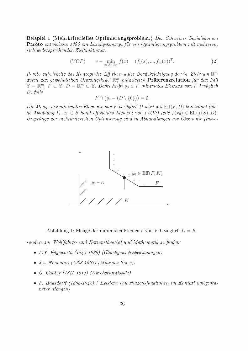
!"#$"!% & '(!)*+*",!*"!%%!# -$,"."!*/01#$*23%!.45 !" # %&!'(!" #)('*+,-).)/67*!,2 !.0&' -!+0! 1234 !'. 5,67.86-).(!90 :;" !'. <90'/'!"7.869")=+!/ /'0 /!%"!"!.>6' % &'?!"69"! %!.?!. @'!+:7.-0').!.(V OP ) v − min

x∈S⊂Rn

f(x) = (f1(x), ..., fm(x))T . !"A*"!0) !.0&' -!+0! ?*6 B).(!90 ?!" CD('!.( 7.0!" E!"; -6' %0'87.8 ?!" '/ @'!+"*7/ Rm?7" % ?!. 8!&,%.+' %!. <"?.7.86-!8!+ R

m+ '.?7('!"0!. 6*89!*!0:*!%7,"20 :;" ?!. F*++

Y = Rm> F ⊂ Y> D = R

m+ ⊂ YG *=!' %!'H0 y0 ∈ F /'.'/*+!6 C+!/!.0 I). F =!(;8+' %

D> :*++6F ∩

(

y0 − (D \ 0))

= ∅. '! J!.8! ?!" /'.'/*+!. C+!/!.0! I). F =!(;8+' % D &'"? /'0 Eff(F,D) =!(!' %.!0 K6'!L%! M=='+?7.8 1NG x0 ∈ S %!'H0 !D('!.0!6 C+!/!.0 I). KO<AN :*++6 f(x0) ∈ Eff(f(S), D)GP"69";.8! ?!" /!%"-"'0!"'!++!. <90'/'!"7.8 6'.? '. M=%*.?+7.8!. (7" Q-).)/'! K'.6=!L

-

6

K!! !! !! !! !!!!

!!

!!

bb

bb

bb

bby0 − K

y0 ∈ Eff(F,K)v

F

#$$%&'()* +, -.)*. './ 0%)%01&.) 2&.0.)3. 45) F $.67*&% 9 D = K:6).?!"! (7" R)%+:*%"06L 7.? S70(!.60%!)"'!N 7.? J*0%!/*0'- (7 T.?!.U• FGVG C?8!&)"0% K12WXL13Y4N KZ+!' %8!&' %06=!?'.87.8!.N• [GIG S!7/*.. K13\]L13X^N KJ'.'/*_L#`0(!NG• ZG a*.0)" K12WXL1312N K 7" %6 %.'0066*0(N• FG b*76?)"c K1242L13WYN K C_'60!.( I). S70(!.6:7.-0').!. '/ B).0!_0 %*+=8!)"?L.!0!" J!.8!.N ;<

• !"! #$%& '()*+,())-. '/012&34&30& 56% 120 7829:0&; <=82<=>0% 7>0<0&:0 2& ?=>@,30$%1&0:0& 0&30&A $?&0 =45 B4:;0&954&C:2$&0& ;4%6 C;43%0250&E F$<2&=&;0230&,9 ?=5:0&.!G< 0H;20&:0 7>0<0&:0 x0 ∈ S '<2: f(x0) ∈ Eff(f(S),Rm+). 109 I%$@>0<9 'JKI. ;4 L&10&AM0%N0&10: <=& $5: 9C=>=%0 7%9=:;O%$@>0<0 <2: PC=>=%2920%4&3954&C:2$&=>0& M$< QRO '(.!P$ @0:%= ?:0& I=9 $>0::2 4&1 P0%=L&2 'M3>! S(+. 5$>30&109 7%9=:;O%$@>0<

min t !"4&:0% /0= ?:4&3 10% B0@0&@012&34&30&f(x) ∈ a+ tk0 − R

m+ ,

x ∈ S,

t ∈ R'<2: I=%=<0:0%& a, k0 ∈ RmA k0 ∈ 2&: R

m+ . ;4% /09:2<<4&3 M$& UV94&30& 109 I%$@>0<9'JKI.! !"#$"!% & W& "@?=&1>4&30& ;4% XC$&$<20 M0%N0&10: U40&@0%30% S(Y 02&0 =&30>, '$10%F0L;2:,. Z4&C:2$& @0;63>2 ? 10% <V3>2 ?0& I%$14C:<0&30 Y ⊂ R

m 4&1 g ∈ Rm+ \ 0[

σ(g; y) := infξ ∈ R | y − ξg ∈ Y,/$&&2990=4A \$%&0: S] '56% 10& Z=>> g = (1, . . . , 1). 4&1 U40&@0%30% S(Y @0;02 ?&0& 12090Z4&C:2$& =4 ? =>9 ^$?>:_:23C02:9,Z4&C:2$&! !"#$"!% ' ()"*+*,-+./!-+."012 W< =%C$N2:;, $10>> '()Y]. 'M3>! "@9 ?&2:: `!]. N0%,10& 3>02 ?;02:23 7%N=%:4&39N0%: 109 a0:4%&9 4&1 120 J=%2=&; $O:2<20%:! F=<2: >203: 02&/2C%2:0%20>>09 KO:2<20%4&39O%$@>0< M$%! G< 120909 ;4 >V90&A C=&& <=& 02&0 PC=>=%2920,%4&3 <2: b2>50 109 Z4&C:2$&=>9 '(. &4:;0&! W& 10% "%@02: M$& "%:;&0% 0: =>! '())). N0%10&Z4&C:2$&=>0 M$< QRO '(. =>9 C$?_%0&:0 a292C$<=c0 'M3>! "@9 ?&2:: `!(. 02&3056?%:! !"#$"!% 3 ()4*0."5*+%+*+%6#"#12 a4@2&$M 4&1 P2&30% S(d 56?%:0& 9$30&=&&:0 :$O2 =>Z4&C:2$&=>0 02& 'M3>! b=<0> S(-.! F=@02 ?02c: 02& Z4&C:2$&=> ψ : Rn → R∪+∞∪−∞?02c: .5$" +% 30&=4 1=&&A N0&& 09 R

n+,<$&$:$& 29: 4&1 ψ(y + tk0) = ψ(y) − t <2:

k0 = (1, 1, ..., 1)T ∈ Rn 0%56>>:! F2090 Z4&C:2$&=>0 4&1 =4 ? 1=9 2&C$N9C2,Z4&C:2$&=>@0;63>2 ? 02&0% 0&30 D 9:0?0& 2& /0;20?4&3 ;4< $@0& 02&3056?%:0& Z4&C:2$&=> ϕD,k0!02:0%?2& 92&1 120 M$& F410C S- @0:%= ?:0:0& "#5.5*" /=&= ?,Z4&C:2$&=>0 M$< QRO 109Z4&C:2$&=>9 ϕD,k0!

!#

!"# $%"&'$(") +,- ./0$#0 1/- 23$4$-")",-/#0 !" #"!$!% &%'!%()%*!% "% (!+ ,"%-%./-01!/-0"2 )%( (!+ 340"/"!+)%* 5!%60"*0 /-%5!70"//0! 8"*!%7 1-:0!% (!+ ;2-$-+"7"!+)%*7:)%20"<%-$!= >"+ 5!0+- 10!% !"%!% $"%!-+!% 0<?4<$<*"7 1!% @-)/ YA B ⊂ Y )%( !"% ;2-$-+"7"!+)%*7:)%20"<%-$ ϕ : Y → R∪−∞∪+∞/"0 B!"%"*!% (!+C :<$*!%(!% 8"*!%7 1-:0!%D(Aϕ1) E-7 ,)%20"<%-$ ϕ "70 B?/<%<0<%A (=1= y, w ∈ YA y ∈ w−B "/4$"."!+0 ϕ(y) ≤ ϕ(w)=(Aϕ1′) E-7 ,)%20"<%-$ ϕ "70 70+"20 B?/<%<0<%A (=1= y, w ∈ YA y ∈ w− (B \ 0) "/4$"."!+0

ϕ(y) < ϕ(w)=(Aϕ2) E-7 ,)%20"<%-$ ϕ "70 2<%#!F=(Aϕ2′) E-7 ,)%20"<%-$ ϕ "70 7)5$"%!-+=(Aϕ2′′) E-7 ,)%20"<%-$ ϕ "70 $"%!-+=(Aϕ3) E-7 ,)%20"<%-$ ϕ 5!7"0.0 ("! G+-%7$-0"<%7?8"*!%7 1-:0

∀s ∈ R, ∀y ∈ Y : ϕ(y + sk0) = ϕ(y) + s. BHC(Aϕ4) E-7 ,)%20"<%-$ ϕ "70 )%0!+1-$570!0"*=(Aϕ4′) E-7 ,)%20"<%-$ ϕ "70 70!0"*=5 6$(+,'$(") +, !"0,#) +$7(,#>"+ 5!0+- 10!% "% (!% :<$*!%(!% ;I0.!% !"%!% +!!$$!% -%- 1?@-)/ Y= E"! &)77-*!%(!7 ;-0.!7 J '!+(!% "% KL :N+ $"%!-+! 0<4<$<*"7 1! @I)/! Y *!.!"*0 B#*$= -) 1 KJOC= 877!"!% D ⊂ Y !"%! %" 10$!!+! P!%*! )%( k0 ∈ Y \ 0A 7<(-77

D + R+k0 ⊆ D. BQCE-%% (!R%"!+!% '"+ (-7 ,)%20"<%-$ ϕD,k0 : Y → R∪−∞∪+∞ B#*$= &55"$()%* SC

ϕD,k0(y) := inft ∈ R | y ∈ tk0 −D. BTC>"+ #!+!"%5-+!% inf ∅ = +∞=U% :<$*!%(!/ ;-0. '!+(!% 8"*!%7 1-:0!% (!7 ,)%20"<%-$7 ϕ = ϕD,k0 B#*$= BJCA BTCCA ("!:N+ ("! <5!% 5!7 1+"!5!%!% &%'!%()%*!% "% (!+ ,"%-%./-01!/-0"2 )%( .)+ ;2-$-+"7"!+)%*#<% V!20<+<40"/"!+)%*74+<5$!/!% '" 10"* 7"%(A %- 1*!'"!7!%=E-7 ,)%20"<%-$ ϕ 1!"W0 !"*!%0$" 1A '!%% dom ϕ 6= ∅ )%( ϕ %" 10 (!% >!+0 −∞ -%?%"//0= 8"%! G!"$/!%*! D ⊆ Y 1!"W0 !"*!%0$" 1A :-$$7 D 6= ∅A D 6= 0 )%( D 6= Y=XL

!!!!!!!!!!!!!!!!!!!!!!!!!!!!!!!!!!!!!!!!!!!!!!!!!!!!!!!!!!!!!!!!!!!!!!!!!!!!!!!!!!!!!!!!!!!!!!!!!!!!!!!!!!!!!!!!!!!!!!!!!!!!!!!!!!!!!!!!!!!!!!!!!!!!!!!!!!!!!!!!!!!!!!!!!!!!!!!!!!!!!!!!!!!!!!!!!!!!!!!!!!!!!!!!!!!!!!!!!!!!!!!!!!!!!!!!!!!!!!!!!!!!!!!!!!!!!!!!!!!!!!!!!!!!!!!!!!!!!!!!!!!!!!!!!!!!!!!!!!!!!!!!!!!!!!!!!!!!!!!!!!!!!!!!!!!!!!!!!!!!!!!!!!!!!!!!!!!!!!!!!!!!!!!!!!!!!!!!!!!!!!!!!!!!!!!!!!!!!!!!!!!!!!!!!!!!!!!!!!!!!!!!!!!!!!!!!!!!!!!!!!!!!!!!!!!!!!!!!!!!!!!!!!!!!!!!!!!!!!!!!!!!!!!!!!!!!!!!!!!!!!!!!!!!!!!!!!!!!!!!!!!!!!!!!!!!!!!!!!!!!!!!!!!!!!!!!!!!!!!!!!!!!!!!!!!!!!!

!!!!!!!!!!!!!!!!!!!!!!!!!!!!!!!!!!!!!!!!!!!!!!!!!!!!!!!!!!!!!!!!!!!!!!!!!!!!!!!!!!!!!!!!!!!!!!!!!!!!!!!!!!!!!!!!!!!!!!!!!!!!!!!!!!!!!!!!!!!!!!!!!!!!!!!!!!!!!!!!!!!!!!!!!!!!!!!!!!!!!!!!!!!!!!!!!!!!!!!!!!!!!!!!!!!!!!!!!!!!!!!!!!!!!!!!!!!!!!!!!!!!!!!!!!!!!!!!!!!!!!!!!!!!!!!!!!!!!!!!!!!!!!!!!!!!!!!!!!!!!!!!!!!!!!!!!!!!!!!!!!!!!!!!!!!!!!!!!!!!!!!!!!!!!!!!!!!!!!!!!!!!!!!!!!!!!!!!!!!!!!!!!!!!!!!!!!!!!!!!!!!!!!!!!!!!!!!!!!!!!!!!!!!!!!!!!!!!!!!!!!!!!!!!!!!!!!!!!!!!!!!!!!!!

K

tk0 − K

tk0

k0

y

y

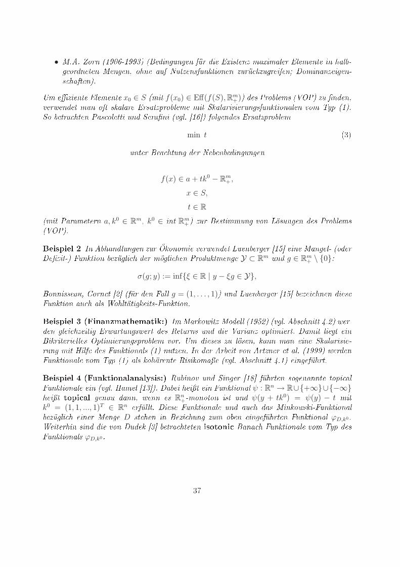
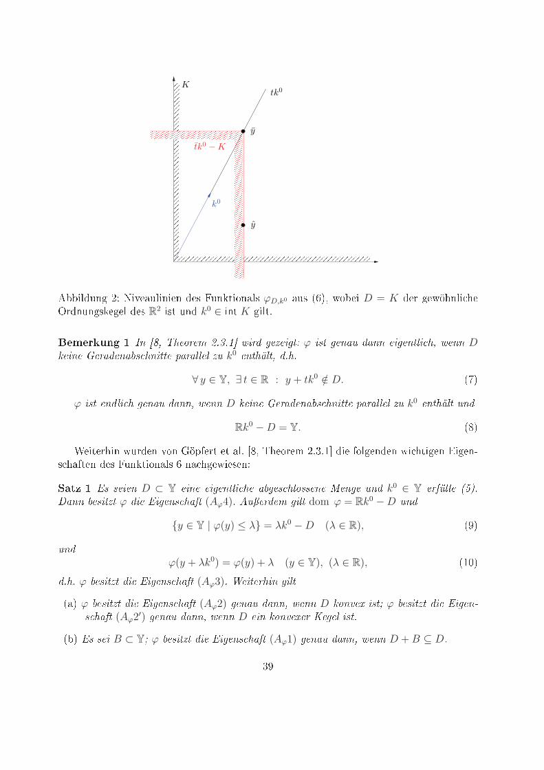
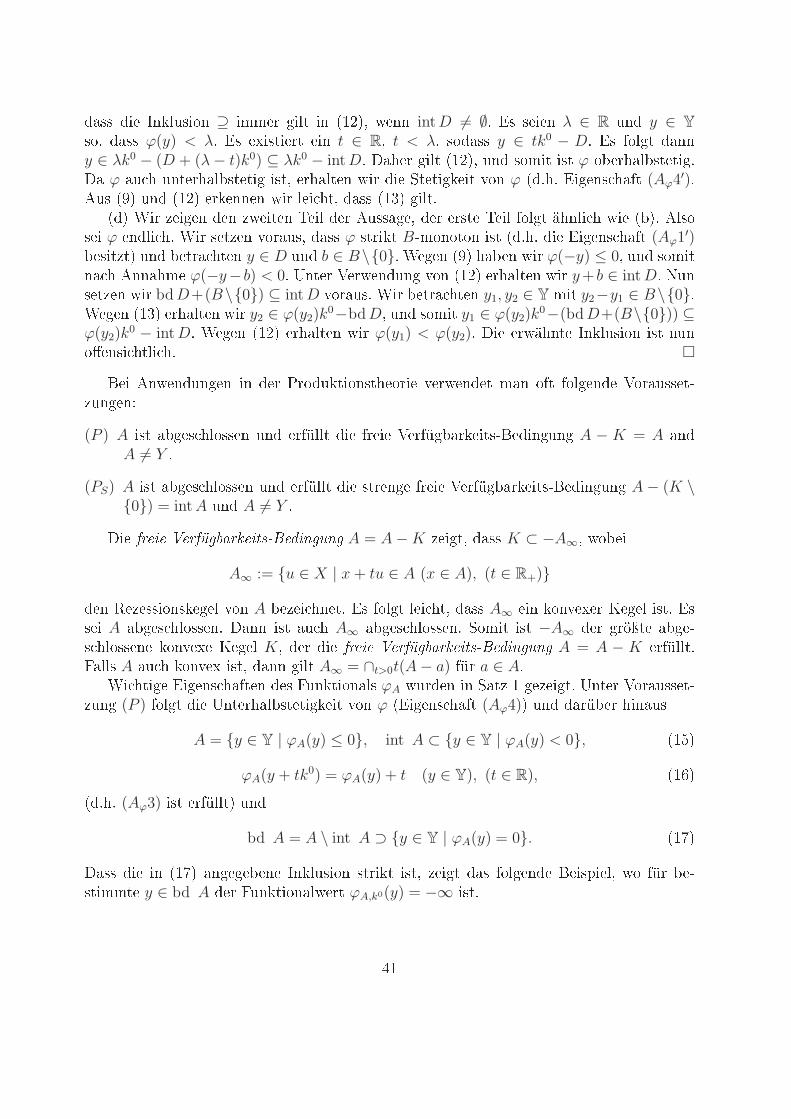
!!"#$%&' () *"+,-%#"&",& $,. /%&01"2&-#. ϕD,k0 -%. 3456 72!," D = K $,8 ',79:&#" :,<8$&%&'.0,',# $,. R2 ".1 %&$ k0 ∈ "&1 K '"#1= !"!#$%&' ( ! "#$ %&'()'* +,-,. 01)2 3'4'1356 ϕ 175 3'!89 28!! '13'!5:1 &$ 0'!! D<'1!' =')82'!8>7 &!155' ?8)8::': 49 k0 '!5&@:5$ 2,&,

∀ y ∈ Y, ∃ t ∈ R : y + tk0 /∈ D. 3>5ϕ 175 '!2:1 & 3'!89 28!!$ 0'!! D <'1!' =')82'!8>7 &!155' ?8)8::': 49 k0 '!5&@:5 9!2

Rk0 −D = Y. 3?5@,"1,8:"& 7%8$,& +2& A9BC,81 ,1 -#= D?6 E:,28,F (=G=H $", C2#',&$,& 7" :1"',& J"',&K. :-C1,& $,. /%&01"2&-#. 4 &- :',7",.,&))*+, ( A7 7'1'! D ⊂ Y '1!' '13'!5:1 &' 8>3'7 &:(77'!' B'!3' 9!2 k0 ∈ Y ')CD::' EFG,H8!! >'71545 ϕ 21' A13'!7 &8C5 (Aϕ4), I9J')2'* 31:5 dom ϕ = Rk0 −D 9!2y ∈ Y | ϕ(y) ≤ λ = λk0 −D (λ ∈ R), 3L59!2ϕ(y + λk0) = ϕ(y) + λ (y ∈ Y), (λ ∈ R), 3HM52,&, ϕ >'71545 21' A13'!7 &8C5 (Aϕ3), K'15')&1! 31:53-5 ϕ >'71545 21' A13'!7 &8C5 (Aϕ2) 3'!89 28!!$ 0'!! D <(!L'M 175N ϕ >'71545 21' A13'!O7 &8C5 (Aϕ2′) 3'!89 28!!$ 0'!! D '1! <(!L'M') P'3': 175,3!5 A7 7'1 B ⊂ YN ϕ >'71545 21' A13'!7 &8C5 (Aϕ1) 3'!89 28!!$ 0'!! D +B ⊆ D,GL

!" #$%&$' '(' &(#)%&*! ,D + (0,+∞) · k0 ⊆ intD !!"-."/(#0 1/'' !#% " ϕ #%$%!2 ('1

y ∈ Y | ϕ(y) < λ = λk0 − intD, (λ ∈ R), !$"y ∈ Y | ϕ(y) = λ = λk0 − bdD, (λ ∈ R). !%" &" 3/**# ϕ $!2$'%*! , !#%0 1/'' 4$#!%&% ϕ 1!$ 5!2$'# ,/6% (Aϕ1) 2$'/( 1/'' 7$'' D+B ⊆

D ⇔ bdD + B ⊆ D8 $!%$",!'0 6/**# ϕ $'1*! , !#%0 1/'' 4$#!%&% ϕ 1!$ 5!2$'# ,/6%(Aϕ1′) 2$'/( 1/''0 7$'' D + (B \ 0) ⊆ int D 9⇔ bdD + (B \ 0) ⊆ intD:8 !"!#$% '()*+ ,-+./00*)1/(2 3" 4*)+. 5)*( 67+ &7* 8*(2*

D′ := (y, t) ∈ Y × R | y ∈ tk0 −D.97* ,-+./00*)1/(2 .( D 1*72): &.00 D′ ;-( *<72+.<570 5*= >?< 70): &@5@ A.BB0 (y, t) ∈ D′/(& t′ ≥ t: &.(( 27B) (y, t′) ∈ D′@ >.)0C 5B7 5: A.BB0 y ∈ tk0 − D /(& t′ ≥ t: &.(( A-B2)tk0 − D = t′k0 − [D + (t′ − t)k0] ⊂ t′k0 − D /(& 67+ *+5.B)*( (y, t′) ∈ D′@ 8.( *+D*(()./ 5: &.00 D′ = T−1(D): 6-4*7 T : Y ×R → Y *7( 0)*)72*+ B7(*.+*+ E<*+.)-+ 70): &*F(7*+)&/+ 5 T (y, t) := tk0−y@ GB0-: A.BB0 D *7( .42*0 5B-00*(*+ D-(;*H*+ I*2*B 70): &.(( 70) ./ 5D′ *7( .42*0 5B-00*(*+ D-(;*H*+ I*2*B@ 9. D′ ;-( *<72+.<570 5*= >?< 70): 4*)+. 5)*( 67+=7) D /(& k0 &7* J/(D)7-( ϕ := ϕD,k0 : Y → R ∪ −∞ ∪ +∞ &*F(7*+) &/+ 5

ϕ(y) := inft ∈ R | (y, t) ∈ D′ = inft ∈ R | y ∈ tk0 −D. !K"L.)M+B7 5 70) &*+ *N*D)7;* 9*F(7)7-(04*+*7 5 ;-( ϕ &7* 8*(2* Rk0 −D /(& D′ ⊂ epiϕ ⊂clD′@ J.BB0 D .42*0 5B-00*( 70): A-B2) 57*+./0 D′ = epiϕ /(& 0-=7) 70) ϕ *7( /()*+5.B40)*O)72*0 J/(D)7-(.B &@5@ (Aϕ4) 27B)": 6*(( D .42*0 5B-00*( 70) /(& dom ϕ = Rk0 −D@L. 5 9*F(7)7-( ;-( ϕ 70) &7* P(DB/07-( ⊇ 7( Q" DB.+: 6C5+*(& &7* /=2*D*5+)* P(DB/07-(./0 &*+ G42*0 5B-00*(5*7) ;-( D A-B2)@ 97* R*17*5/(2 !S" *+5.B)*( 67+ B*7 5) ./0 Q"@ ." 9. &*+ -4*( &*F(7*+)* E<*+.)-+ T 0/+T*D)7; 70) /(& epiϕ = T−1(D) 27B): A-B2) &.00epiϕ *7( D-(;*H*+ I*2*B 70) 2*(./ &.((: 6*(( D = T (epiϕ) &7*0* U72*(0 5.A) 4*07)1)@ 9.0*+274) &7* G/00.2*@ 4" V/(C 50) 0*)1*( 67+ D+B ⊆ D ;-+./0 /(& 4*)+. 5)*( y1, y2 ∈ Y =7) y2 − y1 ∈ B@U0 0*7 t ∈ R 0-&.00 y2 ∈ tk0 − D@ 9.(( 27B) y1 ∈ y2 − B ⊆ tk0 − (D + B) ⊆ tk0 − D:/(& ϕ(y1) ≤ t@ W-=7) 27B) ϕ(y1) ≤ ϕ(y2)@ X7+ 0*)1*( (/( ;-+./0: &.00 ϕ BO=-(-)-( 70)/(& 4*)+. 5)*( y ∈ D /(& b ∈ B@ G/0 Q" A-B2) ϕ(−y) ≤ 0@ X*2*( (−y) − (−y − b) ∈ B*+5.B)*( 67+: &.00 ϕ(−y − b) ≤ ϕ(−y) ≤ 0: /(& 0-=7) /()*+ ,*+6*(&/(2 ;-( Q" A-B2)−y − b ∈ −D: &@5@ y + b ∈ D@X7+ 0*)1*( (/( ;-+./0: &.00 !!" 27B)@ " U0 0*7 λ ∈ R@ X7+ 4*)+. 5)*( y ∈ λk0 − intD@ X*2*( λk0 − y ∈ intD *H70)7*+)*7( ε > 0: 0-&.00 λk0 − y − εk0 ∈ intD ⊆ D@ 9.5*+ 27B) ϕ(y) ≤ λ − ε < λ: 6.0 1*72):KS

!"" #$ %&'()"#*& ⊇ #++$, -#(. #& /0123 4$&& intD 6= ∅5 6" "$#$& λ ∈ R )& y ∈ Y"*3 !"" ϕ(y) < λ5 6" $7#".#$,. $#& t ∈ R3 t < λ3 "* !"" y ∈ tk0 − D5 6" 8*(-. !&&y ∈ λk0 − (D + (λ− t)k0) ⊆ λk0 − intD5 9!:$, -#(. /0123 )& "*+#. #". ϕ *;$,:!(;".$.#-59! ϕ !) : )&.$,:!(;".$.#- #".3 $,:!(.$& 4#, #$ =.$.#-'$#. >*& ϕ / 5:5 6#-$&" :!8. (Aϕ4′)5?)" /@2 )& /012 $,'$&&$& 4#, ($# :.3 !"" /0A2 -#(.5/ 2 B#, C$#-$& $& C4$#.$& D$#( $, ?)""!-$3 $, $,".$ D$#( 8*(-. E:&(# : 4#$ /;25 ?("*"$# ϕ $& (# :5 B#, "$.C$& >*,!)"3 !"" ϕ ".,#'. BF+*&*.*& #". / 5:5 #$ 6#-$&" :!8. (Aϕ1′);$"#.C.2 )& ;$.,! :.$& y ∈ D )& b ∈ B\05 B$-$& /@2 :!;$& 4#, ϕ(−y) ≤ 03 )& "*+#.&! : ?&&!:+$ ϕ(−y− b) < 05 G&.$, H$,4$& )&- >*& /012 $,:!(.$& 4#, y+ b ∈ intD5 I)&"$.C$& 4#, bdD+(B\0) ⊆ intD >*,!)"5 B#, ;$.,! :.$& y1, y2 ∈ Y +#. y2−y1 ∈ B\05B$-$& /0A2 $,:!(.$& 4#, y2 ∈ ϕ(y2)k

0−bdD3 )& "*+#. y1 ∈ ϕ(y2)k0−(bdD+(B\0)) ⊆

ϕ(y2)k0 − intD5 B$-$& /012 $,:!(.$& 4#, ϕ(y1) < ϕ(y2)5 9#$ $,4E:&.$ %&'()"#*& #". &)&*J$&"# :.(# :5 K$# ?&4$& )&-$& #& $, L,* )'.#*&".:$*,#$ >$,4$& $. +!& *8. 8*(-$& $ H*,!)""$.FC)&-$&M

(P ) A #". !;-$" :(*""$& )& $,8N((. #$ 8,$#$ H$,8N-;!,'$#."FK$ #&-)&- A − K = A !& A 6= Y 5

(PS) A #". !;-$" :(*""$& )& $,8N((. #$ ".,$&-$ 8,$#$ H$,8N-;!,'$#."FK$ #&-)&- A− (K \0) = intA )& A 6= Y 59#$ !"#" $"! %&'(!)"#*+,-".#/&0/& A = A−K C$#-.3 !"" K ⊂ −A∞3 4*;$#

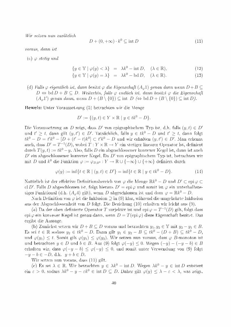
A∞ := u ∈ X | x+ tu ∈ A (x ∈ A), (t ∈ R+) $& O$C$""#*&"'$-$( >*& A ;$C$# :&$.5 6" 8*(-. ($# :.3 !"" A∞ $#& '*&>$7$, P$-$( #".5 6""$# A !;-$" :(*""$&5 9!&& #". !) : A∞ !;-$" :(*""$&5 =*+#. #". −A∞ $, -,QR.$ !;-$F" :(*""$&$ '*&>$7$ P$-$( K3 $, #$ !"#" $"! %&'(!)"#*+,-".#/&0/& A = A − K $,8N((.5S!((" A !) : '*&>$7 #".3 !&& -#(. A∞ = ∩t>0t(A− a) 8N, a ∈ A5B# :.#-$ 6#-$&" :!8.$& $" S)&'.#*&!(" ϕA 4), $& #& =!.C 0 -$C$#-.5 G&.$, H*,!)""$.FC)&- (P ) 8*(-. #$ G&.$,:!(;".$.#-'$#. >*& ϕ /6#-$&" :!8. (Aϕ4)2 )& !,N;$, :#&!)"A = y ∈ Y | ϕA(y) ≤ 0, int A ⊂ y ∈ Y | ϕA(y) < 0, /0T2

ϕA(y + tk0) = ϕA(y) + t (y ∈ Y), (t ∈ R), /0U2/ 5:5 (Aϕ3) #". $,8N((.2 )& bd A = A \ int A ⊃ y ∈ Y | ϕA(y) = 0. /0V29!"" #$ #& /0V2 !&-$-$;$&$ %&'()"#*& ".,#'. #".3 C$#-. !" 8*(-$& $ K$#"W#$(3 4* 8N, ;$F".#++.$ y ∈ bd A $, S)&'.#*&!(4$,. ϕA,k0(y) = −∞ #".5X0

!!!!!!!!!!!!!!!!!!!!!!!!!!!!!!!!!!!!!!!!!!!!!!!!!!!!!!!!!!!!!!!!!!!!!!!!!!!!!!!!!!!!!!!!!!!!!!!!!!!!!!!!!!!!!!!!!!!!!!!!!!!!!!!!!!!!!!!!!!!!!!!!!!!!!!!!!!!!!!!!!!!!!!!!!!!!!!!!!!!!!!!!!!!!!!!!!!!!!!!!!!!!

!!!!!!!!!!!!!!!!!!!!!!!!!!!!!!!!!!!!!!!!!!!!!!!!!!!!!!!!!!!!!!!!!!!!!!!!!!!!!!!!!!!!!!!!!!!!!!!!!!!!!!!!!!!!!!!!!!!!!!!!!!!!!!!!!!!!!!!!!!!!!!!!!!!!!!!!!!!!!!!!!!!!!!!!!!!!!!!!!!!!!!!!!!!!!!!!!!!!!!!!!!!!!!!!!!!!!!!!!!!!!!!!!!!!!!!!!!!!!!!!

K

k0

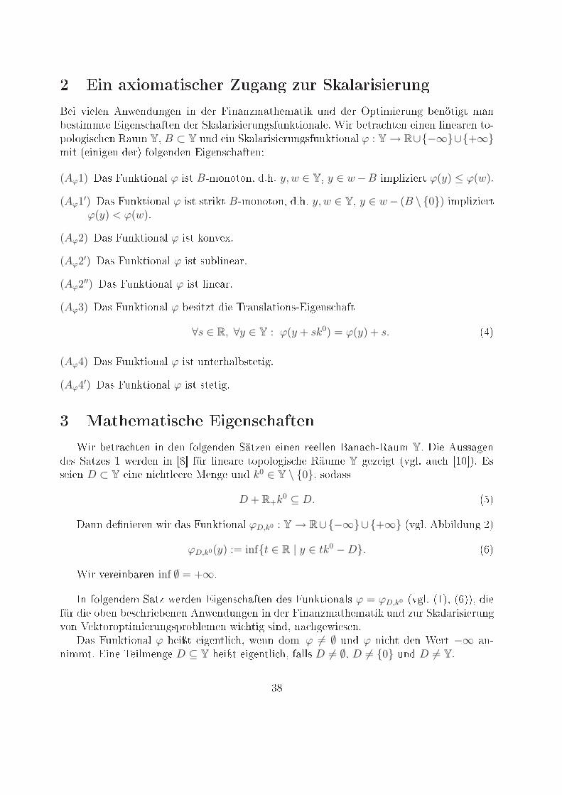
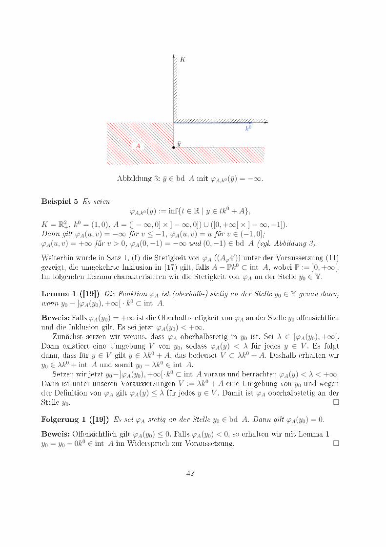
yA !!"#$%&' () y ∈ bd A *"+ ϕA,k0(y) = −∞, !"#$"!% & ! !"#"$ϕA,k0(y) := inft ∈ R | y ∈ tk0 + A,

K = R2+% k0 = (1, 0)% A = (] −∞, 0] × ] −∞, 0]) ∪ ([0,+∞[ × ] −∞,−1])&'($$ )#*+ ϕA(u, v) = −∞ ,-. v ≤ −1% ϕA(u, v) = u ,-. v ∈ (−1, 0]/

ϕA(u, v) = +∞ ,-. v > 0% ϕA(0,−1) = −∞ 0$1 (0,−1) ∈ bd A 23)*& 455#*10$) 67&-."+./0"& 1%/$. "& 23+4 56 789 $". 2+.+"':."+ ;<& ϕA 7(Aϕ4′)9 %&+./ $./ =</3%>>.+4%&' 7559'.4."'+6 $". %*'.:.0/+. ?&:#%>"<& "& 75@9 '"#+6 83##> A− Pk0 ⊂ int A6 1<!." P := ]0,+∞[,?* 8<#'.&$.& A.**3 03/3:+./">"./.& 1"/ $". 2+.+"':."+ ;<& ϕA 3& $./ 2+.##. y0 ∈ Y,'!(() * +,*-/ '#" 80$9+#:$ ϕA #!+ 2:5".;(*5<7 !+"+#) ($ 1". =+"**" y0 ∈ Y )"$(0 1($$%>"$$ y0 − ]ϕA(y0),+∞[ · k0 ⊂ int A& !0!"#1 C3##> ϕA(y0) = +∞ ">+ $". D!./03#!>+.+"':."+ ;<& ϕA 3& $./ 2+.##. y0 <E.&>" 0+#" 0%&$ $". ?&:#%>"<& '"#+, F> >." G.+4+ ϕA(y0) < +∞,H%&I 0>+ >.+4.& 1"/ ;</3%>6 $3>> ϕA <!./03#!>+.+"' "& y0 ">+, 2." λ ∈ ]ϕA(y0),+∞[,J3&& .K">+"./+ ."&. L*'.!%&' V ;<& y06 ><$3>> ϕA(y) < λ 8M/ G.$.> y ∈ V , F> 8<#'+$3&&6 $3>> 8M/ y ∈ V '"#+ y ∈ λk0 + A6 $3> !.$.%+.+ V ⊂ λk0 + A, J.>03#! ./03#+.& 1"/y0 ∈ λk0 + int A %&$ ><*"+ y0 − λk0 ∈ int A,2.+4.& 1"/ G.+4+ y0−]ϕA(y0),+∞[·k0 ⊂ int A ;</3%> %&$ !.+/3 0+.& ϕA(y) < λ < +∞,J3&& ">+ %&+./ %&>./.& =</3%>>.+4%&'.& V := λk0 + A ."&. L*'.!%&' ;<& y0 %&$ 1.'.&$./ J.N&"+"<& ;<& ϕA '"#+ ϕA(y) ≤ λ 8M/ G.$.> y ∈ V , J3*"+ ">+ ϕA <!./03#!>+.+"' 3& $./2+.##. y0, 23%4!5674 * +,*-/ ! !"# ϕA !+"+#) ($ 1". =+"**" y0 ∈ bd A& '($$ )#*+ ϕA(y0) = 0& !0!"#1 DE.&>" 0+#" 0 '"#+ ϕA(y0) ≤ 0, C3##> ϕA(y0) < 06 >< ./03#+.& 1"/ *"+ A.**3 5y0 = y0 − 0k0 ∈ int A "* -"$./>O/% 0 4%/ =</3%>>.+4%&', PQ

! "#$% &' (#) *#+,! -./ 0,%,.0$' 1#22 ϕA 34!5,6 .2$ ((Aϕ2))' 7#882 A ,.!, 34!5,6, 9,!0,.2$: ! ,.!,; 248 *,! =#88 ,/*#8$,! -./ #>2 1,/ "$,$.03,.$ 54! ϕA #! ,.!,/ "$,88, .; !!,/,!1,2 ,?,3$.5,! @,A!.$.4!2+,/,. *,2 1., 843#8, B.C2 *.$%D"$,$.03,.$ 54! ϕA .; !!,/,! .*/,2,?,3$.5,! @,A!.$.4!2+,/,. *,2 dom ϕA (7#882 1#2 =>!3$.4!#8 ,.0,!$8. * .2$): @#/E+,/ *.!#>2'7#882 A = −K >!1 k0 ∈ intK' 1#!! .2$ (-., +,3#!!$) ϕA ,.!, 2$,$.0, 2>+8.!,#/, =>!3$.4!>!1 24;.$ .2$ ϕA B.C2 *.$%D2$,$.0: ; 7480,!1,! "#$% -./1 1., B.C2 *.$%D"$,$.03,.$ 54! ϕA4*!, F4!5,6.$G$254/#>22,$%>!0,! #! A 0,%,.0$: !"# $ %&'(* !"#$%%&'($)* (P ) %&+ &",-..'/(.) 0% *+.'ϕA(y) ≤ ϕA(y′) + ϕ−K(y − y′) (y, y′ ∈ Y). (&H)(..) 1#..% k0 ∈ intK2 3#)) +%' ϕA &)3.+ 5 $)3 6+7% 5+'(8%'&'+* #$, Y/(...) 1#..% y2 ≤K y12 3#)) *+.' ϕA(y2) ≤ ϕA(y1)2 3/5/ ϕA 9&%+'(' 3+& 0+*&)% 5#,' (Aϕ1) ,-"

B = K/(.5) 1#..% A − (K \ 0) ⊂ int A :3#% 9&3&$'&'2 3#%% !"#$%%&'($)* (PS) &",-..' +%'; $)3ϕA &+*&)'.+ 5 +%'2 3#))

[y2 − y1 ∈ −(K \ 0), y1 ∈ dom ϕA] ⇒ ϕA(y2) < ϕA(y1),3/5/ ϕA 9&%+'(' 3+& 0+*&)% 5#,' (Aϕ1′) ,-" B = K/@., *.,/ 0,%,.0$, B.C2 *.$%D"$,$.03,.$ 1,2 =>!3$.4!#82 ϕA ,/;I08. *$ ,.!, J!-,!1>!054! B#0/#!0,D9>8$.C8.3#$4/,!DK,0,8! %>/ L,/8,.$>!0 54! MC$.;#8.$G$2+,1.!0>!0,! 7E/ BID2>!0,! 54! ;,*/3/.$,/.,88,! MC$.;.,/>!02C/4+8,;,! (2.,*, N&O): !"#$"%&"'$" (" %$) *("+",-+./$-+.(0 !" #$%$&'()*+@#2 !. *$8.!,#/, =>!3$.4!#8 (&) .2$ 0,0,+,! 1>/ * ϕ : Y → R ∪ −∞ ∪ +∞ ;.$$,82ϕ(y) := inft ∈ R | y ∈ tk0 −D, (&O)-4+,. Y ,.! /,,88,/ 8.!,#/,/ $4C4840.2 *,/ K#>; .2$ >!1D ⊆ Y' k0 ∈ Y\0'D+R+k

0 ⊆ D:@.,2,2 =>!3$.4!#8 -./1 .! 1,/ =.!#!%;#$*,;#$.3 %>/ Q>#!$.A%.,/>!0 54! K.2.3,! (508:J/$%!,/' @,8+,#!' R+,/ >!1 L,#$* N&' L#;,8 N&S' L,T1, N&U) >!1 .! 5.,8,! #!1,/,!V,+.,$,! 1,/ 9#$*,;#$.3 >!1 1,! W./$2 *#7$2-.22,!2 *#7$,! 0,!>$%$: R.! X,.2C.,8 7E/ ,.!Y,3$4/4C$.;.,/>!02C/4+8,;' -4+,. 1., Z.,87>!3$.4! .! ,.!,! >!,!18. *1.;,!2.4!#8,! K#>;Y 54! Z>7#8825#/.#+8,! #++.81,$' .2$ 1#2 [/4+8,; (Pinvest)' ,.!, +,%E08. * ,.!,/ [/G7,/,!%D/,8#$.4! .! Y 4C$.;#8, (,\%.,!$,) !5,2$.$.4! %> A!1,!: ",$%,! -./ 54/#>2' 1#22 Ω ,.!,9,!0, 54! R8,;,!$#/,/,.0!.22,! .2$ (9,!0, #88,/ #>2 *,>$.0,/ ". *$ ;I08. *,! %>3E!7$.0,!Z>2$G!1,)' 1#!! .2$ ,.! %>3E!7$.0,/' ;.$ ]!2. *,/*,.$ +,*#7$,$,/ Z#*8>!02^>22 #82 R/0,+!.21,/ !5,2$.$.4! ,.!, Z>7#8825#/.#+8, y : Ω → R (%>; X,.2C.,8 1., LI*, ,.!,/ F/,1.$/E 3%#*D8>!0' 1,/ W,/$ ,.!,/ J3$., %> ,.!,; +,2$.;;$,! Z,.$C>!3$): =#882 3,.!, !5,2$.$.4! 0,$G$.0$US

!"#$ #%&& !'( #!)') *+,%--'.%"!%/-) &+--$ 01'!(!.) 21+( 14)'5 '!&# 6) !&&) +&# &)7%(!.)'!&# 8)"-+'()9 :%' ;<'+&7'=1&>)0( !& #!)')4 8)=(1"10(!4!)"+&7'0"1/-)4 !"# #+" ? )!&)@"A,)")&>")-%(!1& !4 B%+4 Y #)" *+,%--'.%"!%/-)& /)' ?"!)/)&$ #!) #+" ? )!&) !"#$%&'"()#'*# D ⊆ Y !&#+>!)"( !"#9 C"(>&)"$ :)-/)%&$ D/)" %&# E)%(? FG ,I?"()& CJ!14) ,I")!&) K)&7) D ⊆ Y .1& *+,%--'.%"!%/-)&$ #!) %=>)0(%/-)& L&.)'(!(!1&)& )&('0") ?)&$ )!&MNCGO y ∈ Y | y(w) ≥ 0 (w ∈ Ω) ⊆ D$ D ∩ y ∈ Y | y(w) < 0 ∀ w ∈ Ω = ∅$NCPO D !'( )!& Q)7)-$NCRO D +D ⊆ D9K)&7)& D ⊆ Y$ #!) #!) CJ!14) NCGOSNCRO ,I" %=>)0(%/-) B!'!=)& )",I--)&$ =<&&)&>+" D!&,I?"+&7 )!&)" @"A,)")&>")-%(!1& !& Y .)" )&#)( )"#)&9 :)" D&(' ?)!#+&7'("A7)"/).1">+7( y1 7)7)&I/)" y2 N#)" T) ?')- .1& y2 >+ y1 !'( )!& %=>)0(%/-)' B!'!=1O 7)&%+#%&&$ )&& y1 − y2 )!& D-)4)&( .1& D !'($ #9?9y1 ≥D y2 ⇐⇒ y1 − y2 ∈ D. NPUO:!) =-)!&'() K)&7)$ #!) NCGOSNCRO )",I--($ !'( D = y ∈ Y | y(w) ≥ 0 ,I" %--) w ∈

Ω9 D!& L&.)'(1" 4!( #!)')" C=>)0(%&>4)&7) !'( %/'1-+( B!'!=1V%/7)&)!7( N"!'!=1V%.)"')O$)" %=>)0(!)"( &+" C&-%7)& 1?&) 8)"-+'() N1#)" 8)"-+'() 4!( T%?"' ?)!&-! ?=)!( 0O9 :!)D!7)&' ?%,()& NCGOSNCRO =<&&)& ,1-7)&#)"4%W)& !&()"0")(!)"( )"#)&M• NCGOM 8)"-+'(-1') C&-%7)& )"#)& !44)" %=>)0(!)"( +&# C&-%7)& 4!( '! ?)")& 8)"V-+'()& )"#)& &!) %=>)0(!)"(9• NCPOM D!& %=>)0(%/-)' B!'!=1 !"# /)-!)/!7 1,( )!&7)7%&7)&9• NCROM K!( > )! %=>)0(%/-)& B!'!=)& !'( %+ ? #!) X+44) %+' #!)')& /)!#)& B!'!=)&%=>)0(%/)-9K!(+&()" !"# ,)'(7)'()--($ #%'' #!) CJ!14) NCPO +&# NCRO &! ?( !44)" '!&&.1-- '!&#$)( % #%&&$ )&& )!& L&.)'(1" &! ?( 4)?" %-' )!&)& /)'(!44()& Y)("%7 %& 6)-# !&.)'(!)")&4< ?()9 L& #!)')4 Z%-- =%&& 4%& #!) CJ!14) NCPO +&# NCRO #+" ? )!& Q1&.)J!(A('VCJ!14)"')(>)& N.7-9 Z<--4)" +&# X ?!)# F[O9:%' Z+&=(!1&%- ϕ !"# !& #)" Z!&%&>4%(?)4%(!= .)" )&#)($ +4 )!& .1"?%&#)&)' B!V'!=1 >+ \+%&(!]>!)")&9 D!& '1- ?)' +,-,!.)&/ /)' ?")!/( )!&)& 6)-#/)("%7$ #)" !4 Z%--).1& 8)"-+'()& #!) X1-.)&> #)' ^&()"&)?4)&' /> 9 #)" Y%&= 4!( ?1?)" T%?"' ?)!&-! ?V=)!( '! ?)"(9 :%/)! '1-- )!&)"')!(' #!) X1-.)&> N,%'(O 7)'! ?)"( +&# %&#)")"')!(' &! ?( >+.!)-Q%0!(%- (1( 7)-)7( )"#)&9 X14!( =%&& )!& B!'!=14%W %-' 4!&!4%-)" Y)("%7 %& 6)-# NQ%0!V(%-O %+,7),%''( )"#)&$ #)" #%>+7)7)/)& )"#)& 4+''$ +4 #!) 7)'%4() L&.)'(!(!1& NB!'!=1O%=>)0(%/)- >+ 4% ?)&9^4 )!& B!'!=14%W /)>I7-! ? #)" C=>)0(%&>4)&7) D ⊆ Y >+ /)' ?")!/)&$ ,I?"()&C"(>&)"$ :)-/)%&$ D/)" +&# E)%(? FG N.)"7-)! ?) E%4)- FGR$ E)_#) FG[O !.012#'%#+,-,!.)&/# )!&$ #9?9 )!&) X=%-%"!'!)"+&7 #)' 8)=(1"10(!4!)"+&7'0"1/-)4' (Pinvest)9[[

!"#$%&'% ()*)+!,-.% *)&/ 01&+')!&-2% µ : Y → R ∪ +∞3 4!5%) Y /%$ 2)&%-$%(-1, /%$ 617-22*8-$)-52%& )*'9 :& /%& ;$5%)'%& 8!& ;$'<&%$3 =%25%-&3 >5%$3 ?%-'" @A1&/ (! +-7%22-$3 D$E-*%83 6-5-$-&+)& @AF 4%$/%& 7!2G%&/% >)G%&* "-7'%& 7H$ +!"#$%&'%()*)+!,-.% G%7!$/%$'IJKAL µ(y + tk0) = µ(y) − t JM$-&*2-')!&*N>)G%&* "-7'L3JKOL µ(0) = 0 1&/ µ(λy) = λµ(y) 7H$ -22% y ∈ Y 1&/ λ > 0 JP!*)')8% ?!,!G%&)'#'L3JKQL µ(y1 + y2) ≤ µ(y1) + µ(y2) 7H$ -22% y1, y2 ∈ Y JR15-//)')8)'#'L3JKSL µ(y1) ≤ µ(y2) 7-22* y1 ≥ y2 JT!&!'!&)%L9=)%*% >)G%&* "-7'%& +-&& ,-& 4)% 7!2G' )&'%$P$%')%$%&I• JKALI =)% M$-&*2-')!&*N>)G%&* "-7' *) "%$'3 /-** /-* ()*)+! /1$ " %)&% <1*#'<2) "%*) "%$% ;&2-G% )& %&'*P$% "%&/%$ ?U"% G%,)2/%$' 4)$/9• JKOLI =)% P!*)')8% ?!,!G%&)'#' 5%*-G'3 /-** /!PP%2'%* ()*)+! /1$ " /!PP%2'%* ()*)+!N+-P)'-2 -5G%*) "%$' 4%$/%& ,1**9• JKQLI =)% R15-//)')8)'#' 5%/%1'%'3 /-** %)&% =)8%$*)V+-')!& /%* ()*)+!* *) " 2!"&'9• JKSLI =)% T!&!'!&)% 5%*-G'3 /-** "U"%$%* ()*)+! ,%"$ ()*)+!+-P)'-2 5%&U')G'9=)% W)8%-1,%&G% Lµ(0) =: D 8!& µ <1, W)8%-1 0 )*' %)& +!&8%X%$ %G%2 1&/ %&'*P$) "'/%$ ;+<%P'-&<,%&G%9 >* +-&& G%<%)G' 4%$/%&3 /-** %)& +!"#$%&'%* ()*)+!,-. /-$G%*'%22'4%$/%& +-&& /1$ "

µ(y) = inft ∈ R | y + tk0 ∈ D. JOALT-& *)%"' 2%) "'3 /-** %)& +!"#$%&'%* ()*)+!,-. ,)' /%, 01&+')!&-2 ϕ(−y) J*)%"% JAYLL)/%&')V<)%$' 4%$/%& +-&& /1$ "ϕ(y) = µ(−y).=-,)' G%2'%& /)% >)G%&* "-7'%& (Aϕ1)3 (Aϕ2)3 (Aϕ3) 1&/ (Aϕ4) /%* 01&+')!&-2* JAYL G%,#.R-'< A %&'*P$% "%&/ 7H$ /-* ()*)+!,-. µ9 >)& ()*)+!,-. µ )&/1<)%$' %)&% ;+<%P'-&<,%&G%J-5"#&G)G 8!& µL

Dµ := y ∈ Y | µ(y) ≤ 0. JOOL=)%*% T%&G% %&'"#2' -22% K!*)')!&%&3 /)% -+<%P'-5%2 *)&/ )& /%, R)&&3 /-** *)% +%)& <1*#'<2)N "%* -P)'-2 %$7!$/%$&9D&'%$ Z%$4%&/1&G /%$ (%*12'-'% )& /%& M"%!$%,%& O9A 1&/ O9O )& [%$'"3 \%)/&%$ @F1&/ ]%,,- F )& [UP7%$'3 M-,,%$3 6^2)&%* 1 @AA +-&& G%<%)G' 4%$/%&3 /-** %)& /1$ " JOALG%G%5%&%* 1&'%$"-25*'%')G%* 01&+')!&-2 ,)'D = y ∈ Y | µ(y) ≤ 0,S_

!" $!% &'! (')!*% $+,-!* ./012./31 4!%'-5-6 &78 $ .901 &!:*'!8- !8&!* ;+** 7*-!8 <!8= !*&7*) >?* +4)!% $"?%%!*!* @;5!A-+*5B!*)!* D6 &'! &'! @C'?B! .@012.@D1 !8,E""!*FG+% 4!&!7-!-6 &+%% &'! (')!*% $+,-!* ./012./31 ,E8 !'* 7*-!8$+"4%-!-')!% H7*;-'?*+" µ)!)!4!* &78 $ .901 )!*+7 &+** !8,E""- %'*&6 !** µ &!:*'!8- '%- &78 $ .901 ,E8 !'*! +4)!=% $"?%%!*! I!*)! D = y ∈ Y | µ(y) ≤ 06 &'! &'! @C'?B! .@012.@D1 !8,E""-FJ4!8&'!%6 '! 4!8!'-% !8 K$*-6 !8&!* '* &!8 H'*+*5B+-$!B+-'; .>)"F HL""B!86 M $'!&N31 &'! @C'?B! .@91 7*& .@D1 B'-7*-!8 !8%!-5- &78 $ !'*! P?*>!C'-K-%>?8+7%%!-57*) +* &'!@;5!A-+*5B!*)!F G+** $+- B+* !*-%A8! $!*&! Q!%7"-+-! ,E8 ;?*>!C! @;5!A-+*5B!*)!*7*& ;?*>!C! Q'%';?B+R!F !" #$%&'()*+,#'-.//S+88T IF I+8;? '-5 !*- ' ;!"-! 0UV9 !'* /?8-,?"'?=WA-'B'!87*)%A8?4"!B6 !" $!% &'! (*-=% $!'&7*)!* !'*!% X*>!%-?8% 8+-'?*+" 4!)8E*&!-F HE8 %!'*! H?8% $7*)%+84!'-!* !8$'!"- I+8=;? '-5 0UUY &!* Z?4!"A8!'% ,E8 ['8-% $+,-% '%%!*% $+,-!*F XB I+8;? '-5=I?&!"" '8& &+=>?* +7%)!)+*)!*6 &+%% X*>!%-?8!* !'*! I+C'B'!87*) &!% \! '**% '$8!8 @*"+)!* +*%-8!4!*7*& )"!' $5!'-') &+% ]'!" $+4!*6 &+% Q'%';? 57 B'*'B'!8!*F G'! X*>!%-?8!* %!-5!* '$8! /?8-=,?"'?% +7% n 7*-!8% $'!&!* @;-'!* 57%+BB!*F (% '8& !'* !"#$%&!'(%"#)'(%** 57)87*&!)!"!)-6 &F$F6 &!8 X*>!%-?8 -8'^- &'! (*-% $!'&7*) 57 _!)'** !'*!8 /!8'?&! 7*& &+8, &'!%! (*-=% $!'&7*) 4'% 57B (*&! &!8 /!8'?&! *' $- >!8K*&!8*F HE8 !'*! %?" $! ,!%-)!"!)-! ]!'-A!8'?&!%?"" P+A'-+" '* &!* n @;-'!* +*)!"!)- !8&!*F ['8 % $8!'4!* xi ∈ R .i ∈ 1, 2, . . . , n1 ,E8&'! @*-!'"!6 !" $! '* &!8 @;-'! i +*)!"!)- !8&!*F G+4!' )'"- ,E8 +""! i ∈ 1, 2, . . . , n xi ≥ 07*& ∑n

i=1xi = 1F G+% P+A'-+"6 !" $!% B+* +7% &!8 @;-'! i *+ $ &!8 ,!%-)!"!)-!* ]!'-A!=8'?&! 578E ;!8$K"- .QE ;)+4! !8- ?&!8 Q!-78*16 4!5!' $*!* '8 B'- Ri6 i ∈ 1, 2, . . . , nFG+4!' $+*&!"- !% %' $ 7B ]7,+""%>+8'+4"!F (% %!'!* x = (x1, ..., xn) &!8 <!;-?8 &!8 @*-!'"!6

µi = E[Ri]6 µ = (µ1, ..., µn)T &!8 <!;-?8 &!8 (8 +8-7*)% !8-! &!8 Q!-78*%6 C = σij

ni,j=1&'! I+-8'C &!8 P?>+8'+*5!* 5 '% $!* &!* Q!-78*% 7*& R = (R1, . . . , Rn)T F G+% Q'%';? &!8)!%+B-!* X*>!%-'-'?* '8& &78 $ &+% Q'%';?B+R +,&!,"-

Var(x) =n

∑

i,j=1

xixjσij = xTCx4!% $8'!4!*6 &!8 \! '** &78 $ &!* (8 +8-7*)% !8- &!% Q!-78*% R(x) =∑n

i=1xiRi6 +"%?&78 $

E[R(x)] =

n∑

i=1

xiµi.Z+-E8"' $ %?"" &!8 \! '** %? )8?R '! BL)"' $ 7*& &+% Q'%';? %? ;"!'* '! BL)"' $ %!'*FG+% ,E$8- +7, !'* !"#!$%#!%&&%' ()$!*!%#+,-')#./&%* B'- 5 !' ]'!",7*;-'?*!*`(PM)

(

−µTxxTCx

)

→ >=B'*7*-!8 _!8E ;%' $-')7*) &!8 Z!4!*4!&'*)7*)!* x ≥ 0 7*& ∑n

i=1xi = 1F3a

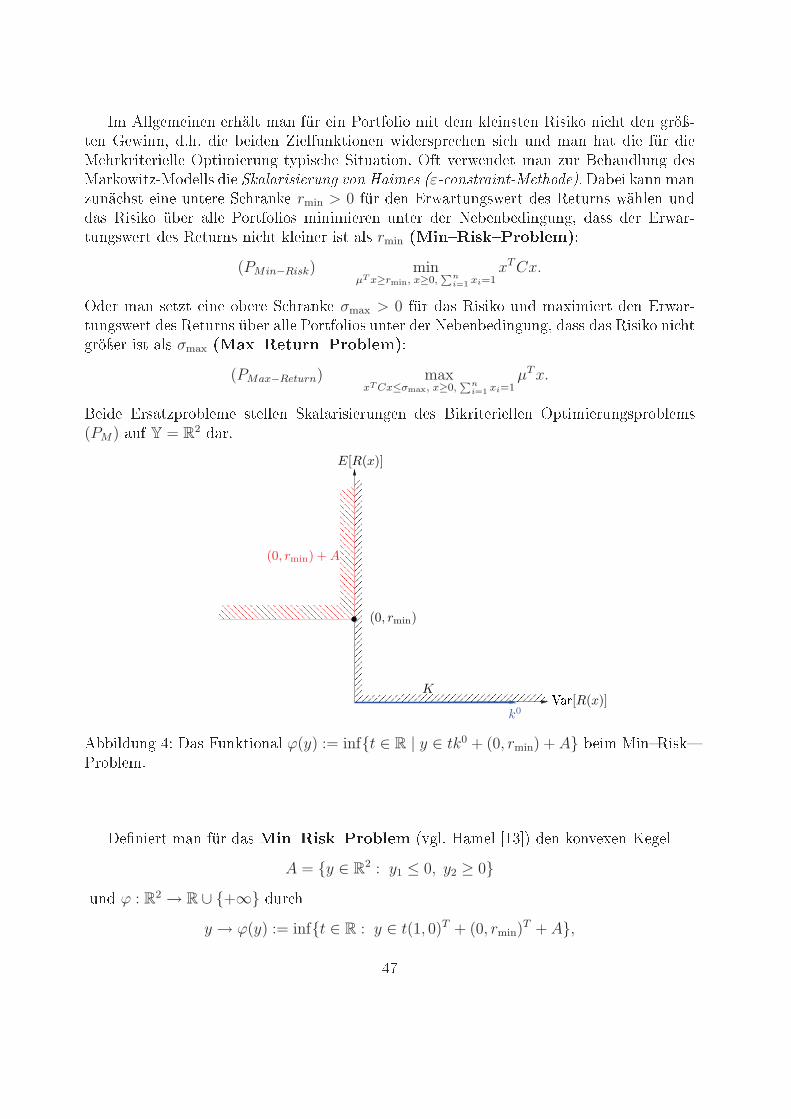
! "##$%!%&'%' %()*#+ !,' -.( %&' /0(+-0#&0 !&+ 1%! 2#%&'3+%' 4&3&20 '& )+ 1%' $(678+%' 9%:&''; 1<)< 1&% =%&1%' >&%#-?'2+&0'%' :&1%(3@(% )%' 3& ) ?'1 !,' ),+ 1&% -.( 1&%A%)(2(&+%(&%##% B@+&!&%(?'$ +C@&3 )% D&+?,+&0'< B-+ E%(:%'1%+ !,' F?( G%),'1#?'$ 1%3A,(20:&+F8A01%##3 1&% !"#"$%&%'$()* +,) -"%.'& /ε0 ,)&2$"%)203'24,5'6< H,=%& 2,'' !,'F?'* )3+ %&'% ?'+%(% D )(,'2% rmin > 0 -.( 1%' I(:,(+?'$3:%(+ 1%3 4%+?('3 :*)#%' ?'11,3 4&3&20 .=%( ,##% /0(+-0#&03 !&'&!&%(%' ?'+%( 1%( J%=%'=%1&'$?'$; 1,33 1%( I(:,(8+?'$3:%(+ 1%3 4%+?('3 '& )+ 2#%&'%( &3+ ,#3 rmin !"#$%"&'$()*+,-./K(PMin−Risk) min

µT x≥rmin, x≥0,∑

n

i=1xi=1

xTCx.B1%( !,' 3%+F+ %&'% 0=%(% D )(,'2% σmax > 0 -.( 1,3 4&3&20 ?'1 !,L&!&%(+ 1%' I(:,(8+?'$3:%(+ 1%3 4%+?('3 .=%( ,##% /0(+-0#&03 ?'+%( 1%( J%=%'=%1&'$?'$; 1,33 1,3 4&3&20 '& )+$(67%( &3+ ,#3 σmax !01$%-23)#$()*+,-./K(PMax−Return) max

xT Cx≤σmax, x≥0,∑

n

i=1xi=1

µTx.G%&1% I(3,+F@(0=#%!% 3+%##%' D2,#,(&3&%(?'$%' 1%3 G&2(&+%(&%##%' B@+&!&%(?'$3@(0=#%!3(PM) ,?- Y = R

2 1,(<

!!!!!!!!!!!!!!!!!!!!!!!!!!!!!!!!!!!!!!!!!!!!!!!!!!!!!!!!!!!!!!!!!!!!!!!!!!!!!!!!!!!!!!!!!!!!!!!!!!!!!!!!!!!!!!!!!!!!!!!!!!!!!!!!!!!!!!!!!!!!!!!!!!!!!!!!!!!!!!!!!!!!!!!!!!!!!!!!!!!!!!!!!!!!!!!!!!!!!!!!!!!!!!!!!!!!!!!!!!!!!!!!!!!!!!!!!!!!!!!!!!!!!!!!!!!!!!!!!!!!!!!!!!!!!!!!!!!!!!!!!!!!!!!!!!!!!!!!!!!!!!!!!!!!!!!!!!!!!!!!!!!!!!!!!!!!!!!!!!!!!!!!!!!!!!!!!!!!!

!!!!!!!!!!!!!!!!!!!!!!!!!!!!!!!!!!!!!!!!!!!!!!!!!!!!!!!!!!!!!!!!!!!!!!!!!!!!!!!!!!!!!!!!!!!!!!!!!!!!!!!!!!!!!!!!!!!!!!!!!!!!!!!!!!!!!!!!!!!!!!!!!!!!!!!!!!!!!!!!!!!!!!!!!

K

E[R(x)]

(0, rmin)

(0, rmin) + A

!"[R(x)]k0"==&#1?'$ MK H,3 N?'2+&0',# ϕ(y) := inft ∈ R | y ∈ tk0 + (0, rmin) + A =%&! A&'O4&32O/(0=#%!<H%P'&%(+ !,' -.( 1,3 !"#$%"&'$()*+,-. QE$#< R,!%# STUW 1%' 20'E%L%' X%$%#

A = y ∈ R2 : y1 ≤ 0, y2 ≥ 0?'1 ϕ : R

2 → R ∪ +∞ 1?( )y → ϕ(y) := inft ∈ R : y ∈ t(1, 0)T + (0, rmin)

T + A,MY

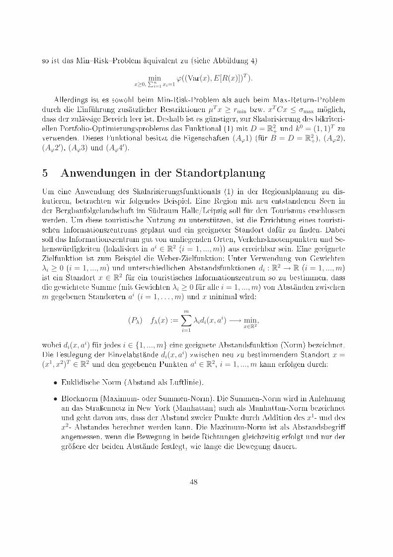
! " # $% &"'()" *(+,!-./0 123"4%./'# 53 6 "/7/ 8--".$3'9 :;min

x≥0,∑

n

i=1xi=1

ϕ((<%,(x), E[R(x)])T ).8../,$"'9 " # / !=!7. -/"0 &"'>)" *>+,!-./0 %. %3 7 -/"0 &%@>)/#3,'>+,!-./0$3, 7 $"/ A"'BC7,3'9 53 1#5." 7/, )/ #,"*#"!'/' µTx ≥ rmin -5=D xTCx ≤ σmax 0E9." 7F$% $/, 53.1 "9/ G/,/" 7 .//, " #D H/ 7%.- " # / 9C' #"9/,F 53, I*%.%," "/,3'9 $/ -"*,"#/,">/../' +!,#B!."!>JK#"0"/,3'9 K,!-./0 $% L3'*#"!'%. 6M; 0"# D = R2+ 3'$ k0 = (1, 1)T 534/,=/'$/'D H"/ / L3'*#"!'%. -/ "#5# $"/ A"9/' 7%B#/' (Aϕ1) 6BC, B = D = R

2+;F (Aϕ2)F

(Aϕ2′)F (Aϕ3) 3'$ (Aϕ4′)D !"#$"%&"'$" (" %$) *+,"%-)+./,"&"'N0 /"'/ 8'=/'$3'9 $/ I*%.%," "/,3'9 B3'*#"!'%. 6M; "' $/, )/9"!'%.K.%'3'9 53 $" >*3#"/,/'F -/#,% 7#/' =", B!.9/'$/ G/" K"/.D A"'/ )/9"!' 0"# '/3 /'# #%'$/'/' I//' "'$/, G/,9-%3B!.9/.%'$ 7%B# "0 IC$,%30 O%../PQ/"K5"9 !.. BC, $/' R!3," 03 /, 7.! /'=/,$/'D N0 $"/ / #!3," #" 7/ S3#53'9 53 3'#/, #C#5/'F " # $"/ A,," 7#3'9 /"'/ #!3," #"> 7/' T'B!,0%#"!' 5/'#,30 9/K.%'# 3'$ /"' 9//"9'/#/, I#%'$!,# $%BC, 53 U'$/'D H%-/" !.. $% T'B!,0%#"!' 5/'#,30 93# 4!' 30."/9/'$/' J,#/'F </,*/7, *'!#/'K3'*#/' 3'$ I/>7/' =C,$"9*/"#/' 6.!*%." "/,# "' ai ∈ R2 6i = 1, ..., m;; %3 /,,/" 7-%, /"'D A"'/ 9//"9'/#/V"/.B3'*#"!' " # 530 G/" K"/. $"/ W/-/,>V"/.B3'*#"!'X N'#/, </,=/'$3'9 4!' Y/=" 7#/'

λi ≥ 0 6i = 1, ..., m; 3'$ 3'#/, 7"/$." 7/' 8- #%'$ B3'*#"!'/' di : R2 → R 6i = 1, ..., m;" # /"' I#%'$!,# x ∈ R

2 BC, /"' #!3," #" 7/ T'B!,0%#"!' 5/'#,30 ! 53 -/ #"00/'F $% $"/ 9/=" 7#/#/ I300/ 60"# Y/=" 7#/' λi ≥ 0 BC, %../ i = 1, ..., m; 4!' 8- #1'$/' 5=" 7/'m 9/9/-/'/' I#%'$!,#/' ai (i = 1, . . . , m) 3'$ x 0"'"0%. =",$X

(Pλ) fλ(x) :=m

∑

i=1

λidi(x, ai) −→ min

x∈R2

,=!-/" di(x, ai) BC, Z/$/ i ∈ 1, ..., m /"'/ 9//"9'/#/ 8- #%'$ B3'*#"!' 6S!,0; -/5/" 7'/#DH"/ L/ #./93'9 $/, A"'5/.%- #1'$/ di(x, a

i) 5=" 7/' '/3 53 -/ #"00/'$/0 I#%'$!,# x =(x1, x2)T ∈ R

2 3'$ $/' 9/9/-/'/' +3'*#/' ai ∈ R2F i = 1, ..., m *%'' /,B!.9/' $3, 7X

• A3*."$" 7/ S!,0 68- #%'$ %. Q3B#."'"/;D• G.! *'!,0 6&%@"030> !$/, I300/'>S!,0;D H"/ I300/'>S!,0 =",$ "' 8'./7'3'9%' $% I#,%[/''/#5 "' S/= \!,* 6&%'7%##%'; %3 7 %. &%'7%##%'>S!,0 -/5/" 7'/#3'$ 9/7# $%4!' %3 F $% $/, 8- #%'$ 5=/"/, +3'*#/ $3, 7 8$$"#"!' $/ x1> 3'$ $/ x2> 8- #%'$/ -/,/ 7'/# =/,$/' *%''D H"/ &%@"030>S!,0 " # %. 8- #%'$ -/9,"]%'9/0/ /'F =/'' $"/ G/=/93'9 "' -/"$/ )" 7#3'9/' 9./" 75/"#"9 /,B!.9# 3'$ '3, $/,9,E[/,/ $/, -/"$/' 8- #1'$/ B/ #./9#F ="/ .%'9/ $"/ G/=/93'9 $%3/,#D:^

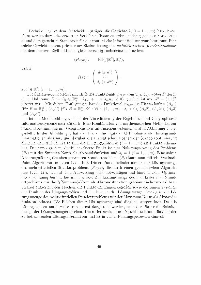
!"#$"! %$&!"'( ") *"+ ,-() /"!*0-')(#1'"#2 *!" 3"4! /(" λi 5i = 1, ..., m6 7")(80&"'"-9:!")" 4"#*"- *0# / *;) "#4;#("(" <"#="/#);07=%++"- 84!) /"- *"- '"'"$"-"- >(;-*%#("-ai 0-* *"+ '")0 /("- >(;-*%#( x 7?# *;) (%0#!)(!) /" @-7%#+;(!%-)8"-(#0+ $")(!++(9 ,!-")%& /" 3"4! /(0-' "-()A#! /( "!-"# >=;&;#!)!"#0-' *") !"#$#%&!#%!''!( )&*(+,#&-#,.'! /2$"! *"+ +"/#"#" B!"&70-=(!%-"- '&"! /$"#" /(!'( -"$"-"!-;-*"# )("/"-C

(PV OP ) : Eff(f [R2],Rm+),4%$"!

f(x) :=

d1(x, a1)

· · ·dm(x, am)

,

x, ai ∈ R22 (i = 1, . . . , m)9:!" >=;&;#!)!"#0-' "#7%&'( +!( !&7" *") D0-=(!%-;&) ϕD,k0 E%+ FGA 5H62 4%$"! D *0# /"!-"- ;&$#;0+ D := y ∈ R

m+ | λ1y1 + ... + λmym ≥ 0 '"'"$"- !)( 0-* k0 = (1, 1)T'")"(8( 4!#*9 I!( *!")"- D")(&"'0-'"- /;( *;) D0-=(!%-;& ϕD,k0 *!" ,!'"-) /;7("- (Aϕ1)57?# B = R

m+ 62 (Aϕ1′) 57?# B = R

m+ 2 7;&&) ∀i ∈ 1, ..., m : λi > 062 (Aϕ2)2 (Aϕ2′′)2 (Aϕ3)0-* (Aϕ4′)9J"! *"# I%*"&&$!&*0-' 0-* $"! *"# <!)0;&!)!"#0-' *"# ,#'"$-!))" )!-* 3"%'#;A/!) /"@-7%#+;(!%-))G)("+" )"/# -?(8&! /9 ,!-" K%+$!-;(!%- E%- +;(/"+;(!) /"- I"(/%*"- 80#>(;-*%#($")(!++0-' +!( 3"%'#;A/!) /"- @-7%#+;(!%-))G)("+"- 4!#* !- L$$!&*0-' M *;#N'")("&&(9 @- *"# L$$!&*0-' M /;( *"# O&;-"# *!" *!'!(;&"- P#(/%A/%(%) ;&) !-("#'#0-*N!-7%#+;(!%-"- ;=(!E!"#( 0-* *;#?$"# *!" (/"+;(!) /"- ,$"-"- *"# >(;-*%#(%A(!+!"#0-'"!-'"$&"-*"(9 L07 *"# K;#(" )!-* *!" ,!-';-')'#QR"- ai 5i = 1, ..., m6 ;&) O0-=(" "#="--N$;#9 :"# "(4;) '#QR"#"2 *0-="& +;#=!"#(" O0-=( !)( "!-" S1/"#0-')&Q)0-' *") O#%$&"+)

(Pλ) +!( *"# >0++"-NS%#+ ;&) L$)(;-*)70-=(!%- 0-* λi = 1 5i = 1, ..., m69 ,!-" )%& /"S1/"#0-')&Q)0-' *") %$"- '"-;--("- >(;-*%#(A#%$&"+) (Pλ) =;-- +;- +!(("&) O#%T!+;&NO%!-(NL&'%#!(/+0) "#/;&("- 5E'&9 UHV69 :!")"# O0-=( $"X-*"( )! / !- *"# YQ)0-')+"-'"*") +"/#=#!("#!"&&"- >(;-*%#(A#%$&"+) (PV OP )2 *!" *0# / "!-"- '"%+"(#!) /"- L&'%#!(/N+0) 5E'&9 UHZ62 *"# ;07 "!-"# L0)4"#(0-' "!-"# -%(4"-*!'"- 0-* /!-#"! /"-*"- PA(!+;N&!(1()$"*!-'0-' $"#0/(2 $")(!++( 40#*"9 B0# YQ)0-')+"-'" *") +"/#=#!("#!"&&"- >(;-*N%#(A#%$&"+) +!( *"# l15>0++"-6NS%#+ ;&) L$)(;-*)70-=(!%- '"/Q#"- *!" /%#!8%-(;& $849E"#(!=;& ;0)'"#! /("("- D&1 /"-2 *!" O0-=(" *"# ,!-';-')'#QR"- )%4!" *!" Y!-!"- 84!) /"-*"- O0-=("- *"# ,!-';-')'#QR"- 0-* *"- D&1 /"- *"# YQ)0-')+"-'"9 L-;&%' !)( *!" YQN)0-')+"-'" *") +"/#=#!("#!"&&"- >(;-*%#(A#%$&"+) +!( *"# I;T!+0+NS%#+ ;&) L$)(;-*)N70-=(!%- )! /($;#9 :!" D&1 /"- *!")"# YQ)0-')+"-'" )!-* *!;'%-;& ;0)'"#! /("(9 :; ;&&"YQ)0-')[1 /"- ;-("!&)4"!)" (#;-)A;#"-( *;#'")("&&( 4"#*"-2 =;-- *"# O&;-"# *!" > /-!((N+"-'" *"# YQ)0-')+"-'"- "#)"/"-9 :!")" J"(#; /(0-' "#+Q'&! /( *!" ,!-) /#1-=0-' *"#80 $"(#; /("-*"- YQ)0-');&("#-;(!E"- 0-* !)( !- E!"&"- O&;-0-')A#%8"))"- )!--E%&&9\]

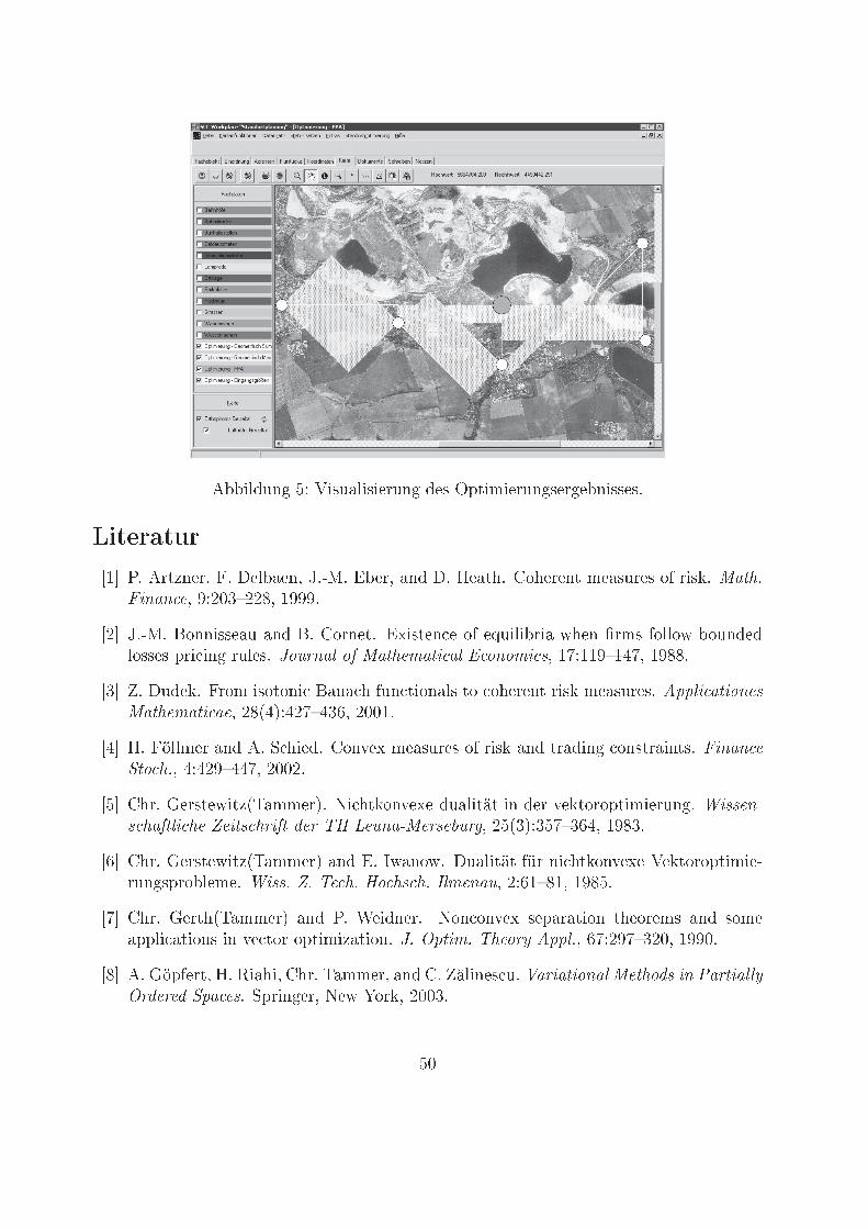
!!"#$%&' () *"+%,#"+"-.%&' $-+ /01"2"-.%&'+-.'-!&"++-+3 !"#$%"&$45 73 .18&-.9 :3 ;-#!,-&9 <3=>3 ?!-.9 ,&$ ;3 @-,1A3 BCA-.-&1 2-,+%.-+ CD ."+E3 !"#$%&'!' )9 F)GHIJGGK9 5FFF34G <3=>3 LC&&"++-,% ,&$ L3 BC.&-13 ?M"+1-& - CD -O%"#"!.", PA-& Q.2+ DC##CP !C%&$-$#C++-+ 0." "&' .%#-+3 *+,-'!. +/ !"#)0!"& !. 1 +'+0& 29 5R)55FJ5SR9 5FKK34I T3 ;%$-E3 :.C2 "+C1C&" L,&, A D%& 1"C&,#+ 1C CA-.-&1 ."+E 2-,+%.-+3 344.& !"&+')2 !"#)0!"& !)9 GKUSV)SGRJSIW9 GHH534S @3 :X##2-. ,&$ 3 Y A"-$3 BC&Z-M 2-,+%.-+ CD ."+E ,&$ 1.,$"&' C&+1.,"&1+3 %&'!' )5"+ #$9 S)SGFJSSR9 GHHG34( BA.3 [-.+1-P"18U\,22-.V3 ]" A1EC&Z-M- $%,#"1^1 "& $-. Z-E1C.C01"2"-.%&'3 6&22)'72 #!/".& #) 8)&"2 #-&/" 9)- :; <),'!7 )-2)=,->9 G(UIV)I(RJIWS9 5FKI34W BA.3 [-.+1-P"18U\,22-.V ,&$ ?3 _P,&CP3 ;%,#"1^1 D`. &" A1EC&Z-M- *-E1C.C01"2"-=.%&'+0.C!#-2-3 6&22$ 8$ :) #$ ;+ #2 #$ ?.0)'!,9 G)W5JK59 5FK(34R BA.3 [-.1AU\,22-.V ,&$ 73 a-"$&-.3 ]C& C&Z-M +-0,.,1"C& 1A-C.-2+ ,&$ +C2-,00#" ,1"C&+ "& Z- 1C. C01"2"8,1"C&3 *$ @4"&0$ :#)+-A 344.$9 WR)GFRJIGH9 5FFH34K 3 [X0D-.19 @3 b",A"9 BA.3 \,22-.9 ,&$ B3 Tc#"&-+ %3 B!-&!"&+'!. )"#+92 &' C!-"&!..A@-9)-)9 54! )23 Y0."&'-.9 ]-P dC.E9 GHHI3(H

! #$ %&'()*+, -$ ./)0*/ 2, 340 52*$ -366)*$ !"#$%!&'# ()!*'+,!%-%!%-./+/$ 7/)89):;-)<=4)*, >/)?=30)4, @AA!$ BA #$ %&'()*+, 52*$ -366)*, 340 -$ ./)0*/ 2$ !"#$%!&'# ()!*'+,!%-%!%-./+/$ -)<=4)*,C+<++:3*+, @AA!$ BB #$ %&'()*+, 52*$ -366)*, 340 5$ DEF/4)? <$ # 4)8 6/4/63F 'G/4+ +2)G*)6 /4 '*G0< +?'3 )?$ 01 !%-1 !$#!&)!"#!, BHIJKJLJJA, B!!!$ B@ M$>$ M363 2)*, N$ NF36*G+2, 340 52*$ -366)*$ C+340G*+G'+/6/)*<4:$ O4 P$ Q<0)9*)*, )0/+G*, 2+# 3)!/' &#/ 4,&#--+#5#!/$ 7/)8):;-)<=4)*, >/)?=30)4, BR!LBSK, @AAH$ BR #$ M36)F$ -*34?F3+/T) ?)+? 340 (<4 +/G4? 340 /+? 3''F/ 3+/G4? +G */?U 6)3?<*) +2)G*V340 4G4F/4)3* ?)'3*3+/G4$ 65#75+!'8 4%5'+!9:)';#59<!+=1 >%--#9?+''#!@#5", @AAJ$ BW X$ M)V0)$ 5G2)*)4+ */?U 6)3?<*)? 340 T) +G* G'+/6/Y3+/G4$ O4 N$9M$ NZ()*, M$ .G696)F(34:)*, 52*$ -366)*, 340 N$ >/4UF)*, )0/+G*?, 4)-'+ 5+'#5+% 2# +/+,! 4%*+!" %!&()BB. C./'#D/$ CM#N[., #3 2)4, RLB@, @AAK$ BS \$ %$ Q<)4=)*:)*$ ])8 G'+/63F/+V '*/4 /'F)? (G* ) G4G6/ )^ /)4 V 340 )_</F/=*/<6$E,)5!%- ,F G7'+D+B%'+,! H;#,5. %!& 77-+ %'+,!/, JSI@@BL@KW, B!!@$ BK #$ `3? GF)++/ 340 $ C)*3a4/$ C 3F3*/Y/4: T) +G* G'+/6/Y3+/G4 '*G=F)6?$ E1 G7'1 H;#,5. 77-1, W@IW!!LS@W, B!HW$ BJ .$-$ .G U3()FF3*, C$ b*V3?)T, 340 c$ D3=3*34U/4$ \)T/3+/G4 6)3?<*)? /4 */?U 343FV?/?340 G'+/6/Y3+/G4$ (+!%! # C', ;%/'+ /, BAISBLJW, @AAK$ BH #$c$ .<=/4GT 340 O$ C/4:)*$ -G'/ 3F 340 ?<=9+G'/ 3F (<4 +/G4?$ 0G8483*0 ?)+? 3403=?+*3 + G4T)d/+V$ G7'+D+B%'+,!, SAIRAJLRSB, @AAB$ B! 52*$ -366)* 340 5$ DEF/4)? <$ Q/'? 2/+Y '*G')*+/)? G( +2) ? 3F3*/Y3+/G4 (<4 +/G4 3403''F/ 3+/G4?$ G7'+D+B%'+,!8 ', %77#%5, @AAH$

SB

Reports of the Institutes 2009

01-09. Jan Pruss, Vicente Vergara, Rico Zacher, Well-Posedness and Long-Time Behaviour

for the Non-Isothermal Cahn-Hilliard Equation with Memory

02-09. Siegfried Carl, Patrick Winkert, General comparison principle for variational-hemivariational

inequalities

03-09. Patrick Winkert, L∞−Estimates for Nonlinear Elliptic Neumann Boundary Value

Problems

04-09. Wilma Di Palma, John Neper’s rods: Calculations are boring and tiring! Leon Bat-

tista Alberti’s Cipher Wheel

05-09. Stefan Sperlich, An integration calculus for stochastic processes with stationary in-

crements and spectral density with applications to parabolic Volterra equations

06-09. Stefan Sperlich, A Regularity Theory for Stochastic Processes with Stationary Incre-

ments and Spectral Density with Applications to Anomalous Diffusion

Reports are available via WWW: http://www2.mathematik.uni-halle.de/institut/reports/