Master Thesis

Discrete-time quantum walk on complex networks

for community detection

（量子ウォークによる複雑ネットワークの

コミュニティ検出）

Kanae Mukai

Department of Physics, University of Tokyo

January 29, 2019

Abstract

Many systems such as social networks and biological networks take the form of

complex networks, which have the community structure. Therefore, the commu-

nity detection is of great interest for many researchers. There have been a lot of

studies on community detection that use the classical random walk. The present

study uses the quantum walk instead. The quantum walk has been studied by

many researchers recently. It plays an important role in various fields, especially

in the theory of quantum computers. The discrete-time quantum walk has two

properties: it linearly spreads on a flat space, which is quadratically faster than the

classical random walk; it localizes in some cases because of quantum coherence. We

demonstrate that these properties are useful for community detection on complex

networks. We define the discrete-time quantum walk on complex networks and uti-

lize it for community detection. We numerically show that the quantum walk is

localized in a community to which the initial node belongs. The infinite-time av-

erage of the normalized transition probability between two nodes, calculated from

the eigenvectors, reveals the community structure, indicating that the eigenvec-

tors contain information about localization to communities. We also find that the

infinite-time average reveals the community structure better if the eigenvalues of

the time-evolution unitary matrix are non-degenerate, and hence the Fourier walk

is more suitable for community detection than the Grover walk. Meanwhile, the

probability of the classical random walk on the same network quickly converges to

a stationary distribution. We thus claim that the time average of the probability

of the quantum walk on complex networks reveals the community structure more

explicitly than that of the classical random walk. We also apply our method to two

real-world networks; namely Zachary’s karate-club network and the neural network

of C. elegans. For Zachary’s karate-club network, we show that our method reveals

its community structure correctly. For the neural network of C. elegans, we show

that our result is roughly consistent with that by the modularity-based method.

1

Acknowledgements

Foremost, I would like to show my great appreciation to my supervisor Naomichi Hatano.

He let me choose the research theme freely, and kindly taught the theory of complex

networks and quantum walks from elementary levels. In particular, he taught me about

complex networks in detail. He gave me a lot of opportunities for valuable discussions and

many comments. I could not advance my research without his support. He also taught

me how to make a presentation for my research, and gave many opportunities to talk

about it. I think it is very useful for me when I work at a job.

I also would like to show my great appreciation to Prof. Hideaki Obuse. He taught

me about quantum walks in detail, and gave me many pieces of advice for my research.

I also would like to show my great appreciation to Prof. Masaki Sano and Prof. Takeo

Kato. They read this thesis and gave me many comments. I also would like to thank

many people for many discussions in my poster presentation.

Finally, I would like to show my great appreciation to the other members of the Hatano

laboratory. They gave me many pieces of advice for my research and presentation. I

especially thank Yusuke Tanaka for valuable discussions and comments.

2

Contents

1 Introduction 4

1.1 Quantum walk . . . . . . . . . . . . . . . . . . . . . . . . . . . . . . . . . 4

1.2 Complex networks . . . . . . . . . . . . . . . . . . . . . . . . . . . . . . . 6

2 Quantum walk on complex networks 8

3 Community detection 10

3.1 Infinite-time average . . . . . . . . . . . . . . . . . . . . . . . . . . . . . . 10

3.2 Finite-time calculation . . . . . . . . . . . . . . . . . . . . . . . . . . . . . 18

3.3 Zachary’s karate-club network . . . . . . . . . . . . . . . . . . . . . . . . . 23

3.4 Neural network of C. elegans . . . . . . . . . . . . . . . . . . . . . . . . . . 25

4 Conclusion 31

Appendix A Community data of the neural network of C. elegans 32

3

1 Introduction

1.1 Quantum walk

The quantum walk has been studied in various areas of physics. The quantum walk

is divided into two types: the discrete-time quantum walk [1] and the continuous-time

quantum walk [2]. The time evolution of the latter is expressed by a Hamiltonian obeying

the Schrodinger equation. In the present paper, we focus on the former.

The discrete-time quantum walk is a quantum counterpart of the discrete-time classical

random walk. In the classical random walk e.g. in one dimension, a particle hops to the

left or right stochastically, generating a probability distribution, whereas the quantum

walk is described instead in terms of the probability amplitude of quantum superposition

of the left-mover and the right-mover [1].

Let us present the two-state quantum walk in one dimension as an example. We define

the quantum state at time t on the one-dimensional lattice as

|ψ(t)⟩ =∑x∈Z

∑s=L,R

ψx,s(t) |x⟩ ⊗ |s⟩ , (1.1)

where the internal states |L⟩ and |R⟩ are

|L⟩ =

1

0

, |R⟩ =

0

1

. (1.2)

We normalize the state |ψ(t)⟩ as in

⟨ψ(t)|ψ(t)⟩ =∑x∈Z

∑s=L,R

|ψx,s(t)|2 = 1. (1.3)

The probability of the existence on a site x at time t is

pt(x) =∑s=L,R

|ψx,s(t)|2. (1.4)

The time evolution of the state |ψ(t)⟩ is given by

|ψ(t)⟩ = U |ψ(t− 1)⟩ (1.5)

= U t |ψ(0)⟩ , (1.6)

where the unitary operator U is the product of a shift operator S and a coin operator C:

U = SC. (1.7)

4

The shift operator S is defined as

S =∑x∈Z

(|x− 1⟩ ⟨x| ⊗ |L⟩ ⟨L|+ |x+ 1⟩ ⟨x| ⊗ |R⟩ ⟨R|). (1.8)

In other words, the left-mover |L⟩ hops to the left neighboring site and the right-mover

|R⟩ hops to the right one. In the standard implementation, the left-mover stays so after

the hopping and the right-mover too; in our implementation on the complex network, we

will define an atypical shift operator (2.15) below. In the case of the definition (1.8), the

left-mover would keep moving to the left and the right-mover to the right, which the coin

operator C prevents from happening. The coin operator mixes up the left-mover |L⟩ and

the right-mover |R⟩ on each site as in

C =∑x∈Z

|x⟩ ⟨x| ⊗ Cx, (1.9)

where Cx is

Cx =

a b

c d

. (1.10)

In order to make the matrix U unitary, we set |a|2 + |b|2 = |c|2 + |d|2 = 1.

The quantum walk generally has the following two properties: it linearly spreads on

a flat space and localizes in particular spots [3]. However, quantum walks with different

inner states and different coin operators behave differently. The probability distribution

of the three-state quantum walk in one dimension, for example, has three peaks, one that

moves linearly to the left, one that moves linearly to the right, and the one that localizes

at the initial site [4]. The one of the two-state quantum walk in one dimension, on the

other hand, has only two peaks that spread linearly to the left and right, without any

peak that localizes [5]. In the present thesis, we focus on the two-state walk, using the

Fourier coin and the Grover coin [6, 7]. The walks with these coin operators are called

the Fourier walk and the Grover walk, respectively. We will demonstrate that the two

walks behave differently.

The quantum walk has been applied to quantum computers, search problems and so

on [8, 9, 10]. Many researchers consider that the quantum-mechanical computers could

solve problems more efficiently than the classical computers. The quantum walk has been

already implemented in the laboratory [11].

5

There have been several studies on the quantum walk on networks, mostly on regular

ones [9, 12]. The shift operator and the coin operator have been defined in conformity

to the structure of networks. The quantum walk on networks occupies an important role

on search problems. In general, it takes classical algorithms O(N) steps to identify the

target record from an unsorted database of N records, while it takes quantum mechanical

systems only O(√N) steps [8].

1.2 Complex networks

Many systems such as social networks and biological networks take the form of complex

networks [13]. Representative examples include acquaintance networks [14], the World

Wide Web [15], corporate transaction networks [16], neural networks [17], food webs [18]

and metabolic networks [19].

One characteristic of complex networks is the existence of communities. The com-

munity is a subset of nodes within the network such that connections among the nodes

of the community are denser than those among the other nodes [20]. Communities of

complex networks may be arranged in a hierarchy [13, 20] (see Fig. 1, for example). At

the center of each community is typically a node with many links, which we call a hub.

When we depict the community structure as a tree, which is called a dendrogram in the

social sciences [20] (see Fig. 2, for example), the leaves correspond to the nodes and the

branches to the links. A node at a high level of the dendrogram is likely to be a hub. As

the dendrogram implies, a complex network typically has many nodes with low degrees

and a small number of nodes with high degrees, namely hubs. Several researches show

that the distribution of the degrees follows a power-law or exponential form [21].

Another characteristic is a property called the small-world effect [13, 22]. This means

that the average distance between nodes in a complex network is surprisingly shorter

than that in a random network. The small-world effect is also related to the community

structure; a path that goes through hubs of communities can shorten the distance between

two nodes in different communities. It is thus of great importance to identify communities

from a large set of network data.

There are several algorithms for community detection [13, 20, 23, 24, 25]. The conven-

tional method is the hierarchical clustering [13, 20, 23, 26]. In this method, one calculates

6

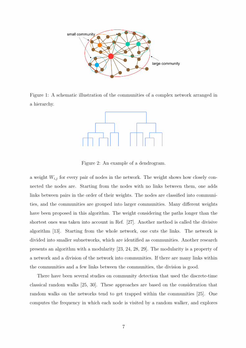
Figure 1: A schematic illustration of the communities of a complex network arranged in

a hierarchy.

Figure 2: An example of a dendrogram.

a weight Wi,j for every pair of nodes in the network. The weight shows how closely con-

nected the nodes are. Starting from the nodes with no links between them, one adds

links between pairs in the order of their weights. The nodes are classified into communi-

ties, and the communities are grouped into larger communities. Many different weights

have been proposed in this algorithm. The weight considering the paths longer than the

shortest ones was taken into account in Ref. [27]. Another method is called the divisive

algorithm [13]. Starting from the whole network, one cuts the links. The network is

divided into smaller subnetworks, which are identified as communities. Another research

presents an algorithm with a modularity [23, 24, 28, 29]. The modularity is a property of

a network and a division of the network into communities. If there are many links within

the communities and a few links between the communities, the division is good.

There have been several studies on community detection that used the discrete-time

classical random walks [25, 30]. These approaches are based on the consideration that

random walks on the networks tend to get trapped within the communities [25]. One

computes the frequency in which each node is visited by a random walker, and explores

7

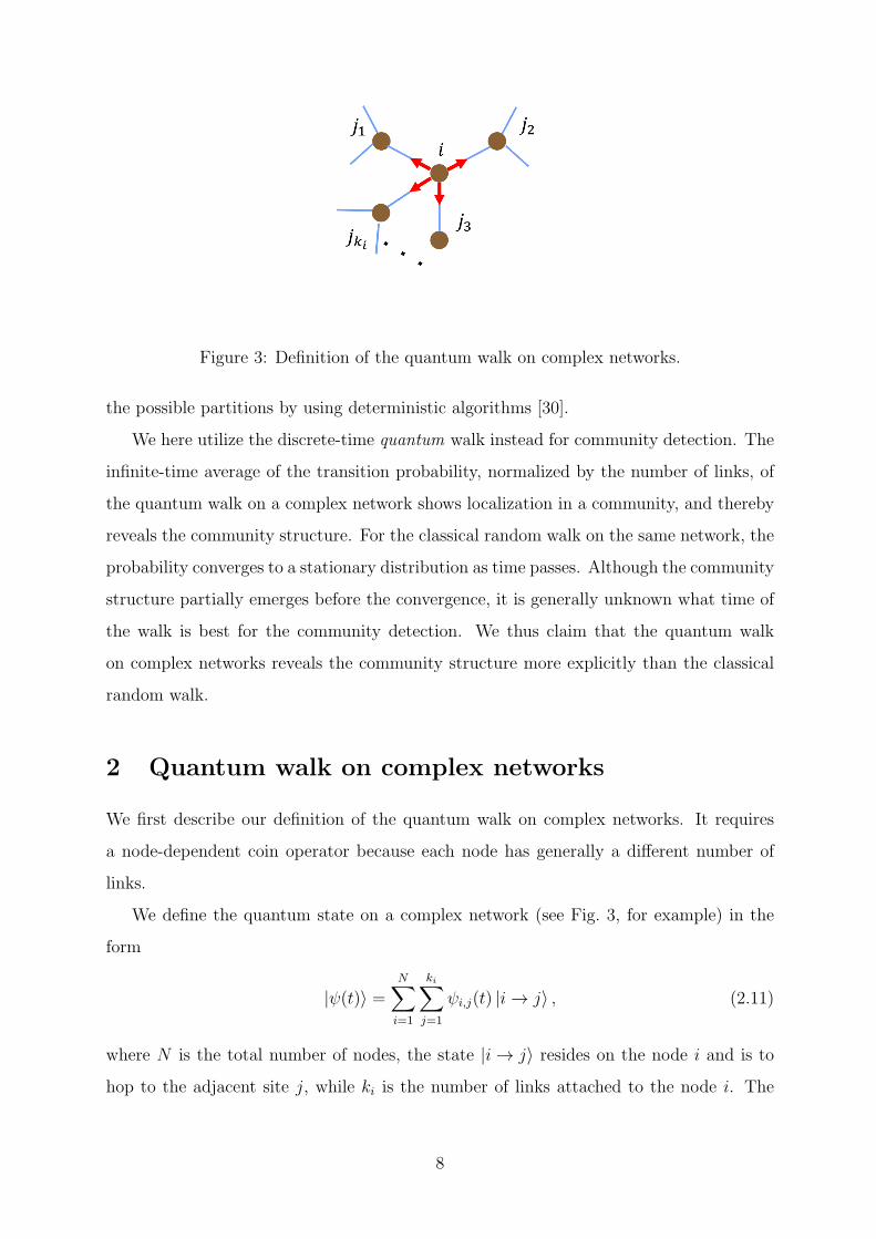
Figure 3: Definition of the quantum walk on complex networks.

the possible partitions by using deterministic algorithms [30].

We here utilize the discrete-time quantum walk instead for community detection. The

infinite-time average of the transition probability, normalized by the number of links, of

the quantum walk on a complex network shows localization in a community, and thereby

reveals the community structure. For the classical random walk on the same network, the

probability converges to a stationary distribution as time passes. Although the community

structure partially emerges before the convergence, it is generally unknown what time of

the walk is best for the community detection. We thus claim that the quantum walk

on complex networks reveals the community structure more explicitly than the classical

random walk.

2 Quantum walk on complex networks

We first describe our definition of the quantum walk on complex networks. It requires

a node-dependent coin operator because each node has generally a different number of

links.

We define the quantum state on a complex network (see Fig. 3, for example) in the

form

|ψ(t)⟩ =N∑i=1

ki∑j=1

ψi,j(t) |i→ j⟩ , (2.11)

where N is the total number of nodes, the state |i→ j⟩ resides on the node i and is to

hop to the adjacent site j, while ki is the number of links attached to the node i. The

8

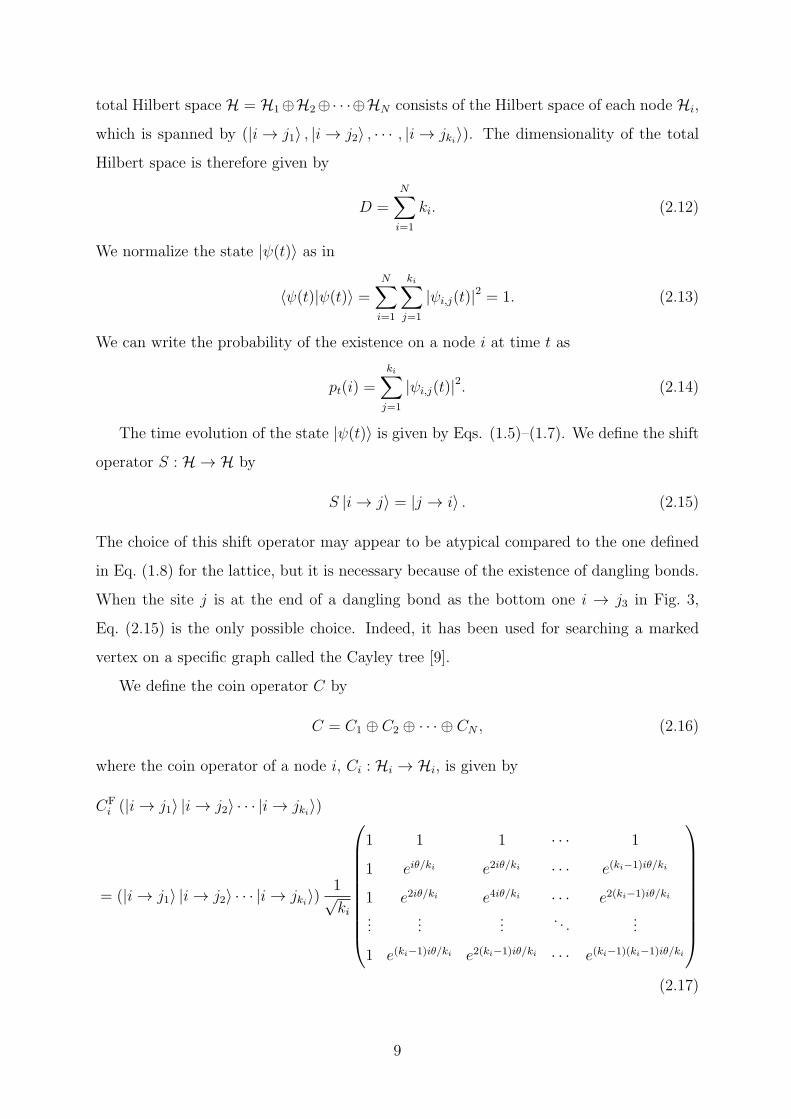
total Hilbert space H = H1⊕H2⊕· · ·⊕HN consists of the Hilbert space of each node Hi,

which is spanned by (|i→ j1⟩ , |i→ j2⟩ , · · · , |i→ jki⟩). The dimensionality of the total

Hilbert space is therefore given by

D =N∑i=1

ki. (2.12)

We normalize the state |ψ(t)⟩ as in

⟨ψ(t)|ψ(t)⟩ =N∑i=1

ki∑j=1

|ψi,j(t)|2 = 1. (2.13)

We can write the probability of the existence on a node i at time t as

pt(i) =

ki∑j=1

|ψi,j(t)|2. (2.14)

The time evolution of the state |ψ(t)⟩ is given by Eqs. (1.5)–(1.7). We define the shift

operator S : H → H by

S |i→ j⟩ = |j → i⟩ . (2.15)

The choice of this shift operator may appear to be atypical compared to the one defined

in Eq. (1.8) for the lattice, but it is necessary because of the existence of dangling bonds.

When the site j is at the end of a dangling bond as the bottom one i → j3 in Fig. 3,

Eq. (2.15) is the only possible choice. Indeed, it has been used for searching a marked

vertex on a specific graph called the Cayley tree [9].

We define the coin operator C by

C = C1 ⊕ C2 ⊕ · · · ⊕ CN , (2.16)

where the coin operator of a node i, Ci : Hi → Hi, is given by

CFi (|i→ j1⟩ |i→ j2⟩ · · · |i→ jki⟩)

= (|i→ j1⟩ |i→ j2⟩ · · · |i→ jki⟩)1√ki

1 1 1 · · · 1

1 eiθ/ki e2iθ/ki · · · e(ki−1)iθ/ki

1 e2iθ/ki e4iθ/ki · · · e2(ki−1)iθ/ki

......

.... . .

...

1 e(ki−1)iθ/ki e2(ki−1)iθ/ki · · · e(ki−1)(ki−1)iθ/ki

(2.17)

9

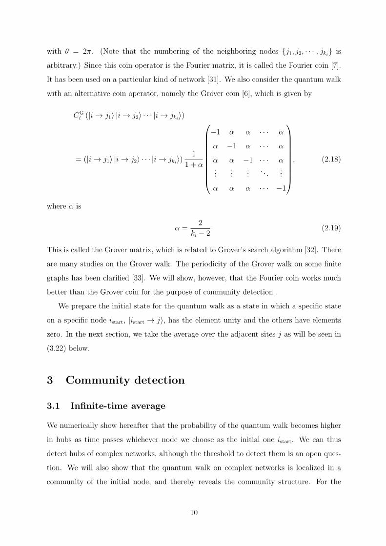
with θ = 2π. (Note that the numbering of the neighboring nodes {j1, j2, · · · , jki} is

arbitrary.) Since this coin operator is the Fourier matrix, it is called the Fourier coin [7].

It has been used on a particular kind of network [31]. We also consider the quantum walk

with an alternative coin operator, namely the Grover coin [6], which is given by

CGi (|i→ j1⟩ |i→ j2⟩ · · · |i→ jki⟩)

= (|i→ j1⟩ |i→ j2⟩ · · · |i→ jki⟩)1

1 + α

−1 α α · · · α

α −1 α · · · α

α α −1 · · · α...

......

. . ....

α α α · · · −1

, (2.18)

where α is

α =2

ki − 2. (2.19)

This is called the Grover matrix, which is related to Grover’s search algorithm [32]. There

are many studies on the Grover walk. The periodicity of the Grover walk on some finite

graphs has been clarified [33]. We will show, however, that the Fourier coin works much

better than the Grover coin for the purpose of community detection.

We prepare the initial state for the quantum walk as a state in which a specific state

on a specific node istart, |istart → j⟩, has the element unity and the others have elements

zero. In the next section, we take the average over the adjacent sites j as will be seen in

(3.22) below.

3 Community detection

3.1 Infinite-time average

We numerically show hereafter that the probability of the quantum walk becomes higher

in hubs as time passes whichever node we choose as the initial one istart. We can thus

detect hubs of complex networks, although the threshold to detect them is an open ques-

tion. We will also show that the quantum walk on complex networks is localized in a

community of the initial node, and thereby reveals the community structure. For the

10

quantum walk on the one-dimensional finite lattice, the probability distribution after a

long period of time has been proved to be stationary and uniform when the quantum walk

behaves symmetrically [34]. For the quantum walk on complex networks, on the other

hand, we here show that the infinite-time average of the normalized transition probability,

calculated from the eigenvectors, shows localization.

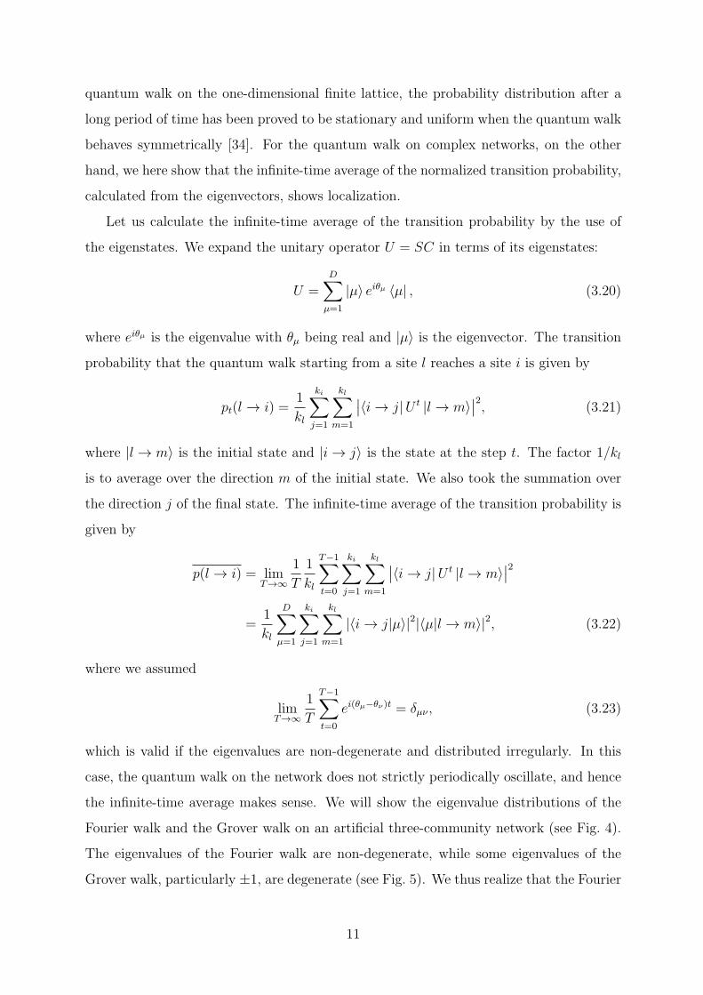
Let us calculate the infinite-time average of the transition probability by the use of

the eigenstates. We expand the unitary operator U = SC in terms of its eigenstates:

U =D∑

µ=1

|µ⟩ eiθµ ⟨µ| , (3.20)

where eiθµ is the eigenvalue with θµ being real and |µ⟩ is the eigenvector. The transition

probability that the quantum walk starting from a site l reaches a site i is given by

pt(l → i) =1

kl

ki∑j=1

kl∑m=1

∣∣⟨i→ j|U t |l → m⟩∣∣2, (3.21)

where |l → m⟩ is the initial state and |i→ j⟩ is the state at the step t. The factor 1/kl

is to average over the direction m of the initial state. We also took the summation over

the direction j of the final state. The infinite-time average of the transition probability is

given by

p(l → i) = limT→∞

1

T

1

kl

T−1∑t=0

ki∑j=1

kl∑m=1

∣∣⟨i→ j|U t |l → m⟩∣∣2

=1

kl

D∑µ=1

ki∑j=1

kl∑m=1

|⟨i→ j|µ⟩|2|⟨µ|l → m⟩|2, (3.22)

where we assumed

limT→∞

1

T

T−1∑t=0

ei(θµ−θν)t = δµν , (3.23)

which is valid if the eigenvalues are non-degenerate and distributed irregularly. In this

case, the quantum walk on the network does not strictly periodically oscillate, and hence

the infinite-time average makes sense. We will show the eigenvalue distributions of the

Fourier walk and the Grover walk on an artificial three-community network (see Fig. 4).

The eigenvalues of the Fourier walk are non-degenerate, while some eigenvalues of the

Grover walk, particularly ±1, are degenerate (see Fig. 5). We thus realize that the Fourier

11

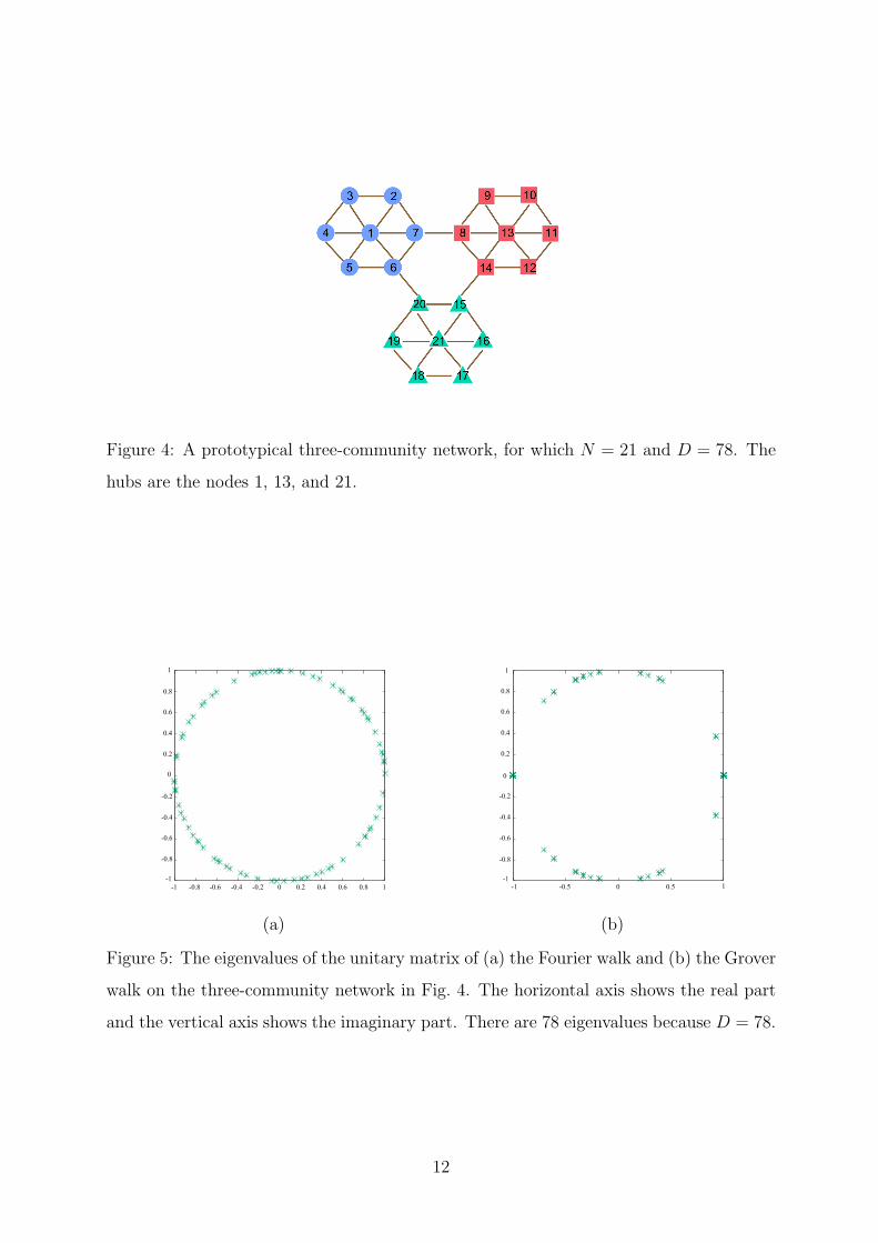
Figure 4: A prototypical three-community network, for which N = 21 and D = 78. The

hubs are the nodes 1, 13, and 21.

1

0.8

0.6

0.4

0.2

0

-0.2

-0.4

-0.6

-0.8

-1-1 -0.8 -0.6 -0.4 -0.2 0 0.2 0.4 0.6 0.8 1

(a)

1

0.6

0.4

0.2

0

-0.2

-0.4

-0.6

-1

-0.8

0.8

-1 -0.5 0 0.5 1

(b)

Figure 5: The eigenvalues of the unitary matrix of (a) the Fourier walk and (b) the Grover

walk on the three-community network in Fig. 4. The horizontal axis shows the real part

and the vertical axis shows the imaginary part. There are 78 eigenvalues because D = 78.

12

1 5 10 15 211

5

10

15

21

0

0.025

0.050

0.075

0.100

0.125

0.150

The target node i

The

initi

al n

ode

l

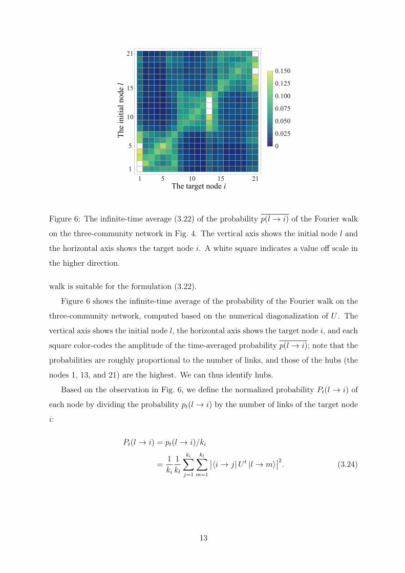
Figure 6: The infinite-time average (3.22) of the probability p(l → i) of the Fourier walk

on the three-community network in Fig. 4. The vertical axis shows the initial node l and

the horizontal axis shows the target node i. A white square indicates a value off scale in

the higher direction.

walk is suitable for the formulation (3.22).

Figure 6 shows the infinite-time average of the probability of the Fourier walk on the

three-community network, computed based on the numerical diagonalization of U . The

vertical axis shows the initial node l, the horizontal axis shows the target node i, and each

square color-codes the amplitude of the time-averaged probability p(l → i); note that the

probabilities are roughly proportional to the number of links, and those of the hubs (the

nodes 1, 13, and 21) are the highest. We can thus identify hubs.

Based on the observation in Fig. 6, we define the normalized probability Pt(l → i) of

each node by dividing the probability pt(l → i) by the number of links of the target node

i:

Pt(l → i) = pt(l → i)/ki

=1

ki

1

kl

ki∑j=1

kl∑m=1

∣∣⟨i→ j|U t |l → m⟩∣∣2. (3.24)

13

1 5 10 15 211

5

10

15

21

0

0.01

0.02

0.03

0.04

0.05

0.06

The target node i

The

initi

al n

ode

l

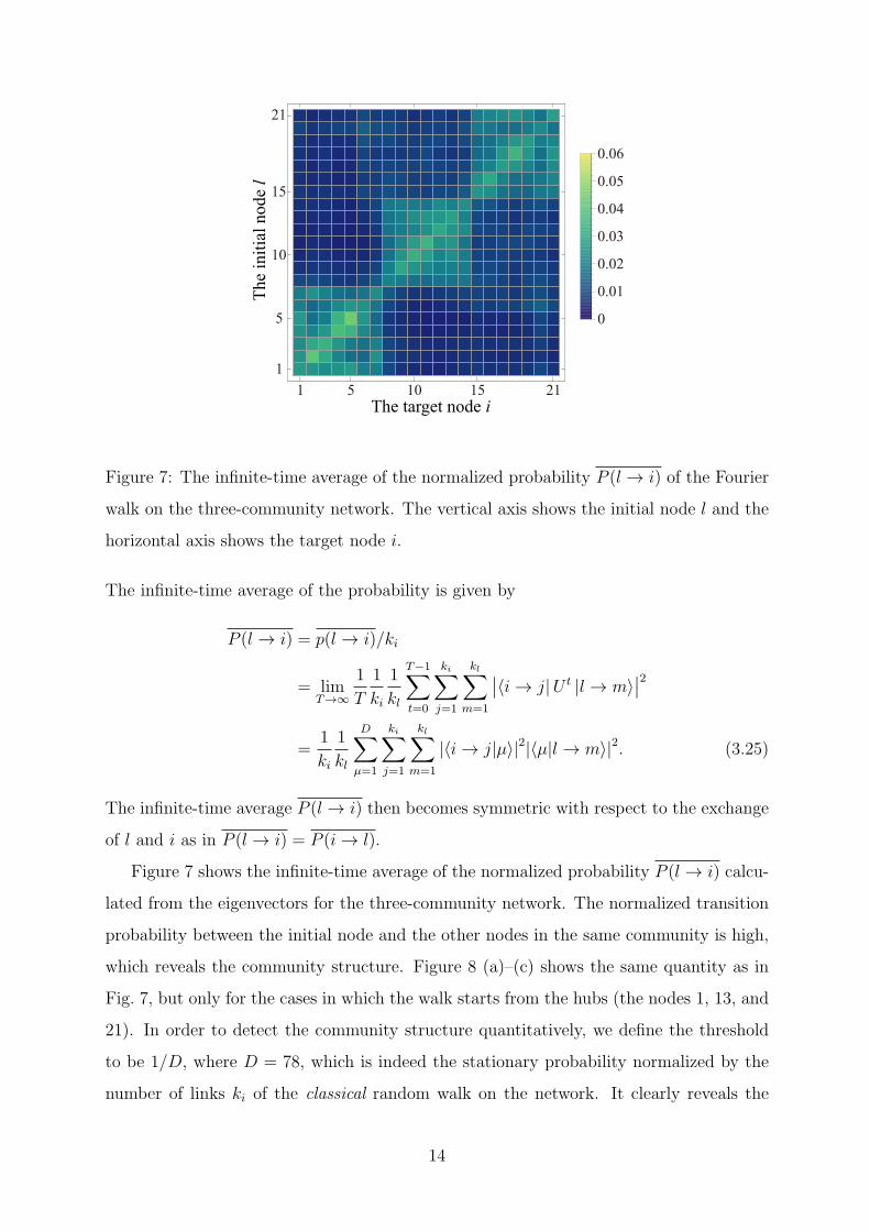
Figure 7: The infinite-time average of the normalized probability P (l → i) of the Fourier

walk on the three-community network. The vertical axis shows the initial node l and the

horizontal axis shows the target node i.

The infinite-time average of the probability is given by

P (l → i) = p(l → i)/ki

= limT→∞

1

T

1

ki

1

kl

T−1∑t=0

ki∑j=1

kl∑m=1

∣∣⟨i→ j|U t |l → m⟩∣∣2

=1

ki

1

kl

D∑µ=1

ki∑j=1

kl∑m=1

|⟨i→ j|µ⟩|2|⟨µ|l → m⟩|2. (3.25)

The infinite-time average P (l → i) then becomes symmetric with respect to the exchange

of l and i as in P (l → i) = P (i→ l).

Figure 7 shows the infinite-time average of the normalized probability P (l → i) calcu-

lated from the eigenvectors for the three-community network. The normalized transition

probability between the initial node and the other nodes in the same community is high,

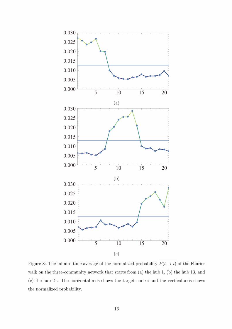
which reveals the community structure. Figure 8 (a)–(c) shows the same quantity as in

Fig. 7, but only for the cases in which the walk starts from the hubs (the nodes 1, 13, and

21). In order to detect the community structure quantitatively, we define the threshold

to be 1/D, where D = 78, which is indeed the stationary probability normalized by the

number of links ki of the classical random walk on the network. It clearly reveals the

14

three communities; the nodes whose probabilities are higher than the threshold belong

to the community whose hub is the initial node. For instance, if the Fourier walk starts

from the hub 1, the probability of the nodes 2, 3, 4, 5, 6, 7, which belong to the same

community, is higher than the threshold. We can thus identify which community each

node belongs to. This shows that the eigenvectors include information about localization

to each community and the quantum walk on the network is localized in a community to

which the initial node belongs.

Let us evaluate the localization of the eigenvectors using the inverse participation ratio

(IPR) [35, 36]. The IPR of an eigenvector

|µ⟩ =N∑i=1

ki∑j=1

ψµ(i, j) |i→ j⟩ (3.26)

is given by

IPR(µ) =

∑Ni=1 pµ(i)

2

(∑N

i=1 pµ(i))2, (3.27)

where the probability pµ(i) is

pµ(i) =

ki∑j=1

|ψµ(i, j)|2. (3.28)

If the eigenvector is sharply localized to one node, the IPR is close to unity in the limit

N → ∞. If the eigenvector is delocalized, the IPR is vanishes as 1/N . If the eigenvector

were localized uniformly in one of the communities of the network in Fig. 4 as in

pµ(i) =

1

7for i = 1, 2, · · · , 7,

0 otherwise,

(3.29)

the IPR would be exactly 1/7 ≈ 0.14.

Figure 9 shows the IPR of each eigenvector for the Fourier walk on the three-community

network. We find that several eigenvectors are localized more strongly than IPR = 1/7.

Figure 10, on the other hand, shows the normalized probability

Pµ(i) =pµ(i)

ki(3.30)

of the Fourier walk on the three-community network. The probability distribution of

each eigenvalue shows the localization. For instance, for the probability distribution of

15

5 10 15 200.000

0.005

0.010

0.015

0.020

0.025

0.030

(a)

5 10 15 200.000

0.005

0.010

0.015

0.020

0.025

0.030

(b)

5 10 15 200.000

0.005

0.010

0.015

0.020

0.025

0.030

(c)

Figure 8: The infinite-time average of the normalized probability P (l → i) of the Fourier

walk on the three-community network that starts from (a) the hub 1, (b) the hub 13, and

(c) the hub 21. The horizontal axis shows the target node i and the vertical axis shows

the normalized probability.

16

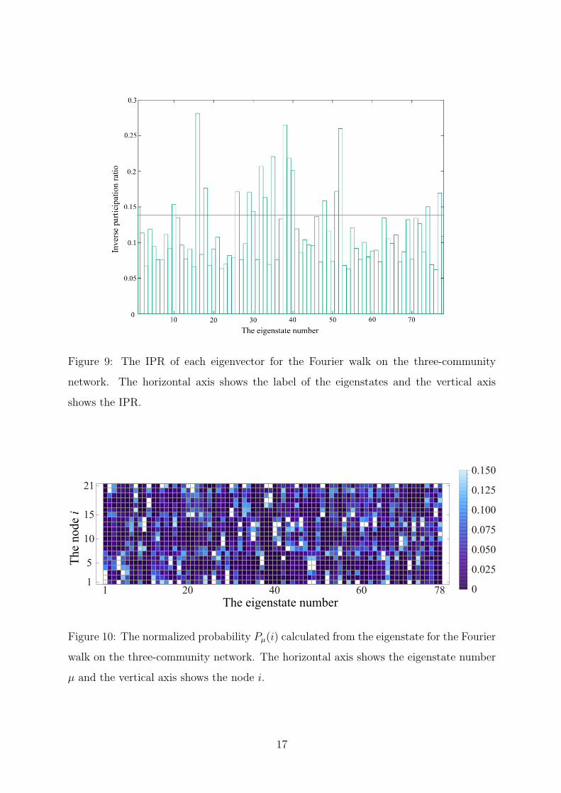
Figure 9: The IPR of each eigenvector for the Fourier walk on the three-community

network. The horizontal axis shows the label of the eigenstates and the vertical axis

shows the IPR.

1 20 40 60 781

5

10

15

21

0

0.025

0.050

0.075

0.100

0.125

0.150

The eigenstate number

The

node

i

Figure 10: The normalized probability Pµ(i) calculated from the eigenstate for the Fourier

walk on the three-community network. The horizontal axis shows the eigenstate number

µ and the vertical axis shows the node i.

17

the eigenstate number 52, the probability for the node 1 and the nodes in the same

community is higher than that of the other nodes; in other words, this eigenvector is

localized in the first community. Similarly, the probability distribution of the eigenstate

number 35 is localized in the second community, and that of the eigenstate number 38 is

localized in the third one. These eigenstates indeed have high values of the IPR in Fig. 9.

The localization of the quantum walk may be related to the Anderson localization.

In the standard sense, the Anderson localization is the property of quantum particles

in random potentials [37, 38]. There are several studies on the Anderson localization of

the discrete-time quantum walk on lattices with randomnes [39, 40]. The quantum walk

on the complex network may be similar to the quantum particle in random potentials

because of the inhomogeneity of the network, and hence may experience the Anderson

localization.

3.2 Finite-time calculation

We next present our finite-time results of the quantum walk on the same three-community

network. We operated the unitary matrix to the initial state |l → m⟩ up to 100 times and

averaged the resulting probability over m.

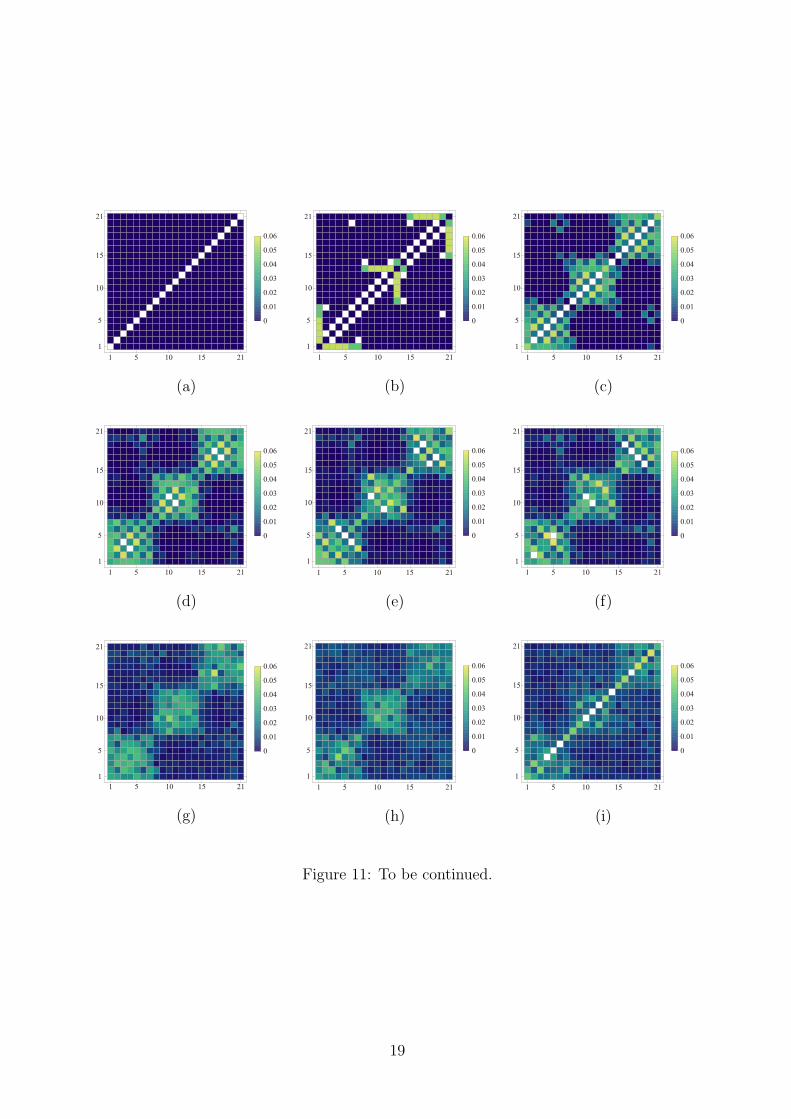
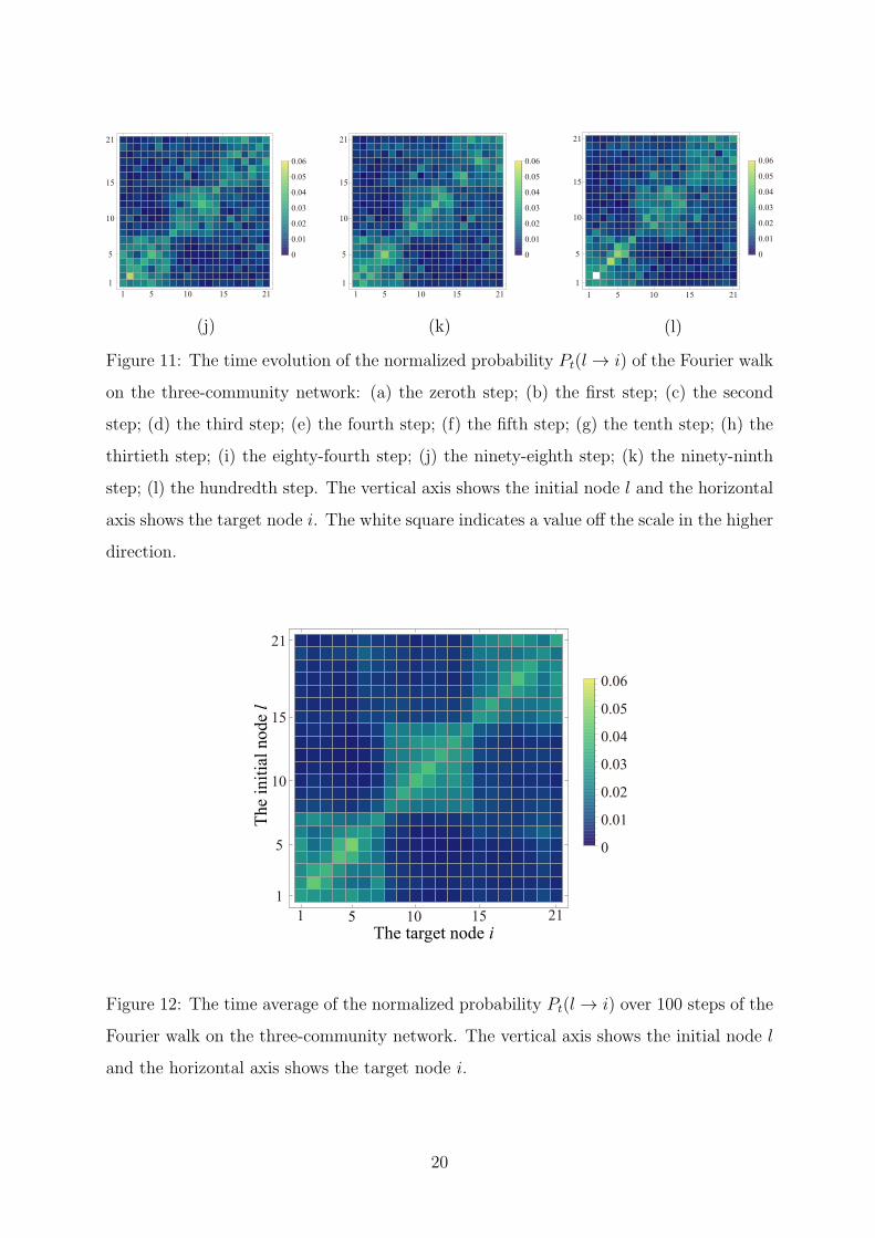
As can be seen from Fig. 11, the Fourier walk behaves roughly periodically but not

completely. Figure 12 shows the time average of the normalized probability Pt(l → i)

over 100 steps from t = 1 through t = 100. It is consistent with Fig. 7, also revealing

the community structure. We can apply this method to complex networks which are too

large to diagonalize the time-evolution unitary matrix U .

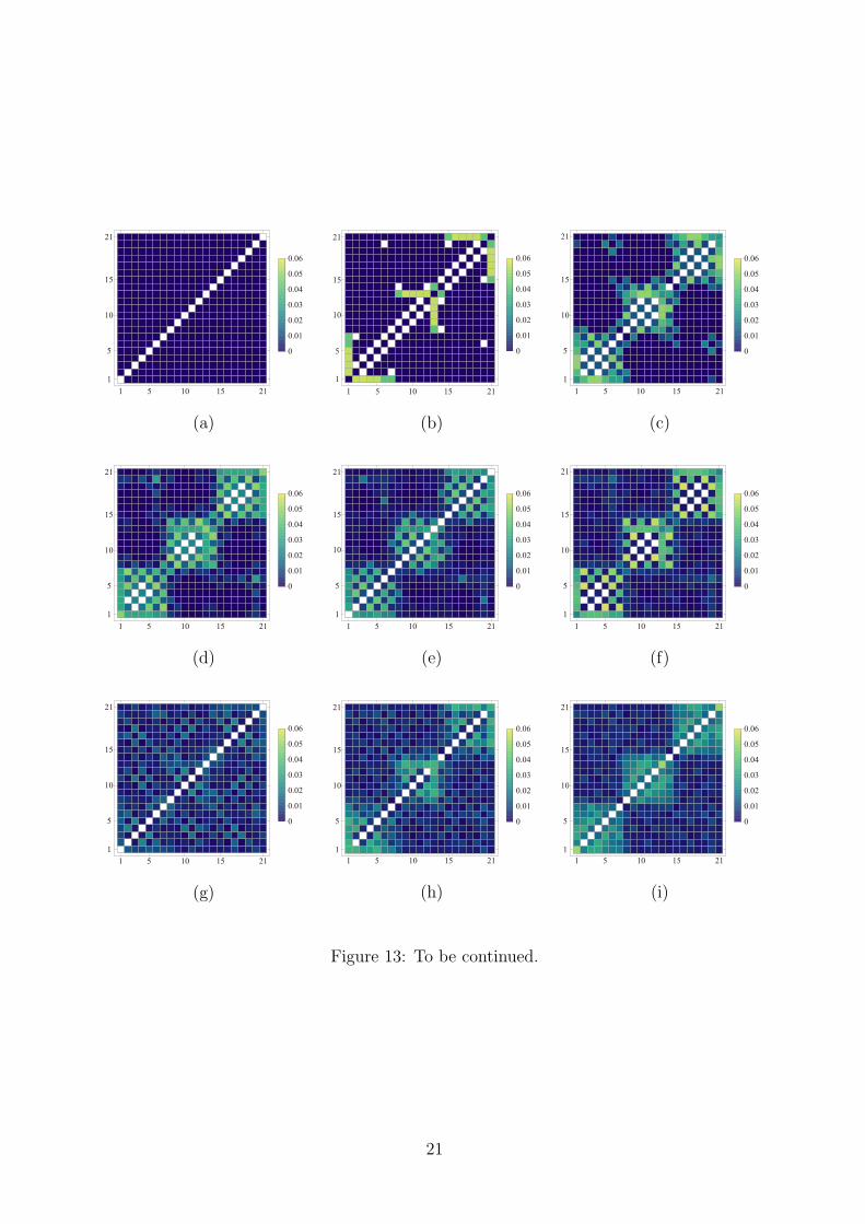
Let us now compare the numerical results of the Fourier walk and the Grover walk.

Figure 13 (a)–(l) shows the normalized probability Pt(l → i) on several steps of the Grover

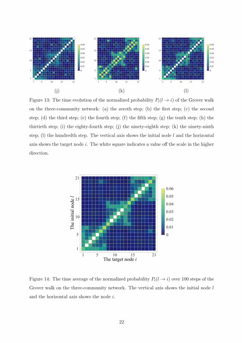
walk on the same network. Figure 14 shows the time average of the normalized probability

Pt(l → i) over 100 steps from t = 1 through t = 100. The normalized probability on the

initial node is high, but that on the other nodes of the same community is relatively low.

Therefore, the Grover walk does not reveal the community structure as clearly as the

Fourier walk does.

Finally, we show in Fig. 15 the normalized probability Pt(l → i) on several steps of

the classical random walk on the same network. The probability of the classical random

18

1 5 10 15 211

5

10

15

21

0

0.01

0.02

0.03

0.04

0.05

0.06

(a)

1 5 10 15 211

5

10

15

21

0

0.01

0.02

0.03

0.04

0.05

0.06

(b)

1 5 10 15 211

5

10

15

21

0

0.01

0.02

0.03

0.04

0.05

0.06

(c)

1 5 10 15 211

5

10

15

21

0

0.01

0.02

0.03

0.04

0.05

0.06

(d)

1 5 10 15 211

5

10

15

21

0

0.01

0.02

0.03

0.04

0.05

0.06

(e)

1 5 10 15 211

5

10

15

21

0

0.01

0.02

0.03

0.04

0.05

0.06

(f)

1 5 10 15 211

5

10

15

21

0

0.01

0.02

0.03

0.04

0.05

0.06

(g)

1 5 10 15 211

5

10

15

21

0

0.01

0.02

0.03

0.04

0.05

0.06

(h)

1 5 10 15 211

5

10

15

21

0

0.01

0.02

0.03

0.04

0.05

0.06

(i)

Figure 11: To be continued.

19

1 5 10 15 211

5

10

15

21

0

0.01

0.02

0.03

0.04

0.05

0.06

(j)

1 5 10 15 211

5

10

15

21

0

0.01

0.02

0.03

0.04

0.05

0.06

(k)

1 5 10 15 211

5

10

15

21

0

0.01

0.02

0.03

0.04

0.05

0.06

(l)

Figure 11: The time evolution of the normalized probability Pt(l → i) of the Fourier walk

on the three-community network: (a) the zeroth step; (b) the first step; (c) the second

step; (d) the third step; (e) the fourth step; (f) the fifth step; (g) the tenth step; (h) the

thirtieth step; (i) the eighty-fourth step; (j) the ninety-eighth step; (k) the ninety-ninth

step; (l) the hundredth step. The vertical axis shows the initial node l and the horizontal

axis shows the target node i. The white square indicates a value off the scale in the higher

direction.

1 10 15 211

5

10

15

21

0

0.01

0.02

0.03

0.04

0.05

0.06

5The target node i

The

initi

al n

ode

l

Figure 12: The time average of the normalized probability Pt(l → i) over 100 steps of the

Fourier walk on the three-community network. The vertical axis shows the initial node l

and the horizontal axis shows the target node i.

20

1 5 10 15 211

5

10

15

21

0

0.01

0.02

0.03

0.04

0.05

0.06

(a)

1 5 10 15 211

5

10

15

21

0

0.01

0.02

0.03

0.04

0.05

0.06

(b)

1 5 10 15 211

5

10

15

21

0

0.01

0.02

0.03

0.04

0.05

0.06

(c)

1 5 10 15 211

5

10

15

21

0

0.01

0.02

0.03

0.04

0.05

0.06

(d)

1 5 10 15 211

5

10

15

21

0

0.01

0.02

0.03

0.04

0.05

0.06

(e)

1 5 10 15 211

5

10

15

21

0

0.01

0.02

0.03

0.04

0.05

0.06

(f)

1 5 10 15 211

5

10

15

21

0

0.01

0.02

0.03

0.04

0.05

0.06

(g)

1 5 10 15 211

5

10

15

21

0

0.01

0.02

0.03

0.04

0.05

0.06

(h)

1 5 10 15 211

5

10

15

21

0

0.01

0.02

0.03

0.04

0.05

0.06

(i)

Figure 13: To be continued.

21

1 5 10 15 211

5

10

15

21

0

0.01

0.02

0.03

0.04

0.05

0.06

(j)

1 5 10 15 211

5

10

15

21

0

0.01

0.02

0.03

0.04

0.05

0.06

(k)

1 5 10 15 211

5

10

15

21

0

0.01

0.02

0.03

0.04

0.05

0.06

(l)

Figure 13: The time evolution of the normalized probability Pt(l → i) of the Grover walk

on the three-community network: (a) the zeroth step; (b) the first step; (c) the second

step; (d) the third step; (e) the fourth step; (f) the fifth step; (g) the tenth step; (h) the

thirtieth step; (i) the eighty-fourth step; (j) the ninety-eighth step; (k) the ninety-ninth

step; (l) the hundredth step. The vertical axis shows the initial node l and the horizontal

axis shows the target node i. The white square indicates a value off the scale in the higher

direction.

1 5 10 15 211

5

10

15

21

0

0.01

0.02

0.03

0.04

0.05

0.06

The target node i

The

initi

al n

ode

l

Figure 14: The time average of the normalized probability Pt(l → i) over 100 steps of the

Grover walk on the three-community network. The vertical axis shows the initial node l

and the horizontal axis shows the node i.

22

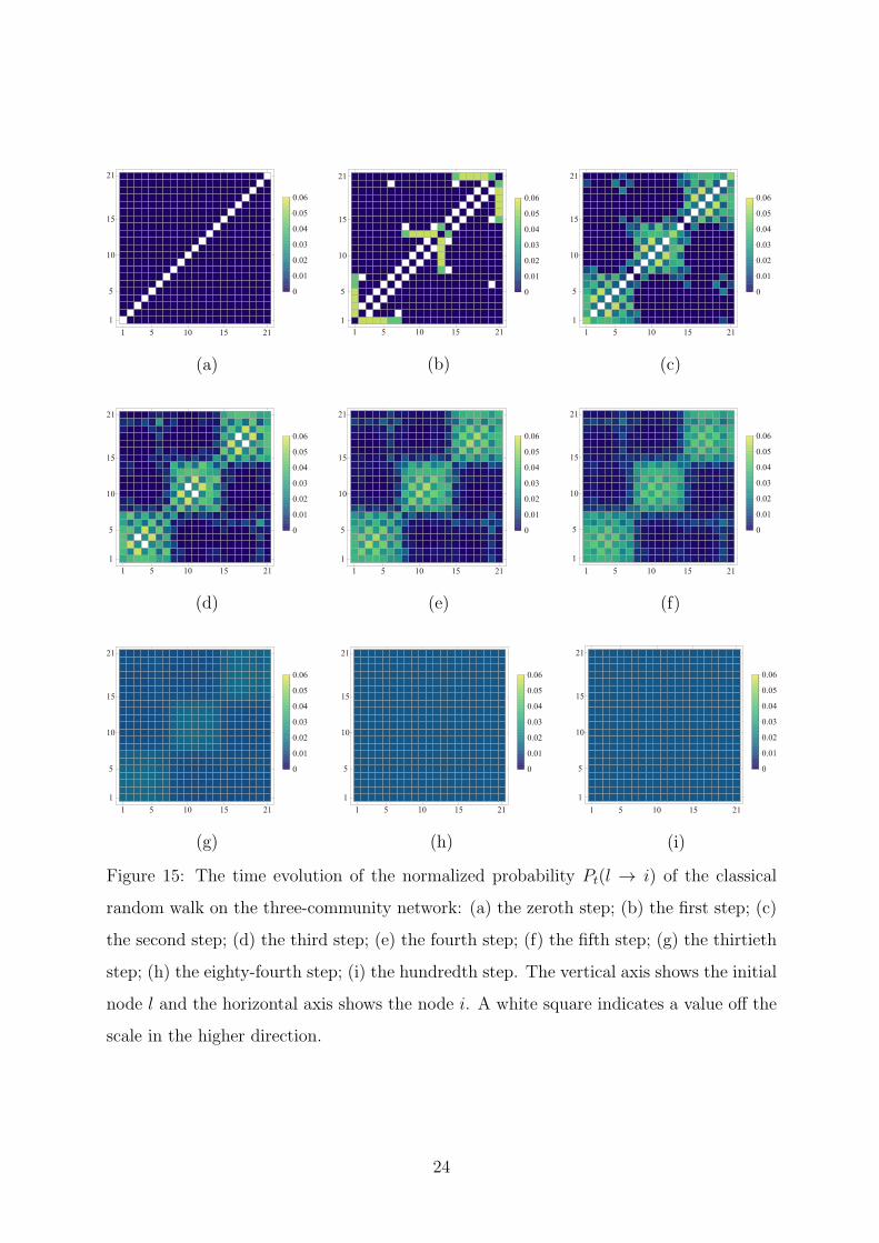
walk quickly converges to the stationary distribution, and hence the infinite-time average

of the probability does not reveal the community structure. For community detection

we have to choose a specific step, which is unknown in general. We thus claim that the

time average of the probability of the quantum walk on complex networks reveals the

community structure more explicitly than that of the classical random walk.

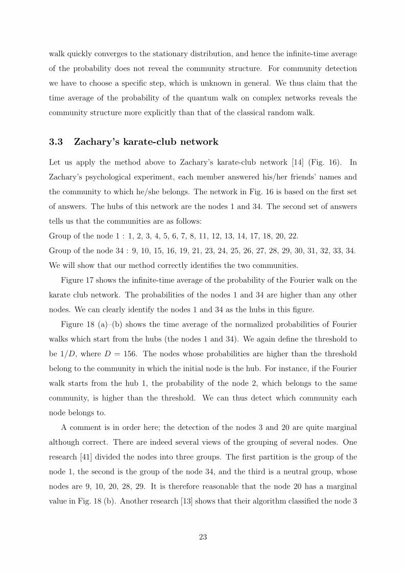
3.3 Zachary’s karate-club network

Let us apply the method above to Zachary’s karate-club network [14] (Fig. 16). In

Zachary’s psychological experiment, each member answered his/her friends’ names and

the community to which he/she belongs. The network in Fig. 16 is based on the first set

of answers. The hubs of this network are the nodes 1 and 34. The second set of answers

tells us that the communities are as follows:

Group of the node 1 : 1, 2, 3, 4, 5, 6, 7, 8, 11, 12, 13, 14, 17, 18, 20, 22.

Group of the node 34 : 9, 10, 15, 16, 19, 21, 23, 24, 25, 26, 27, 28, 29, 30, 31, 32, 33, 34.

We will show that our method correctly identifies the two communities.

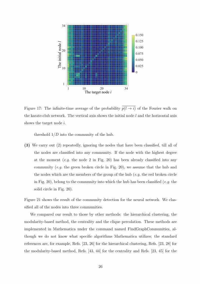
Figure 17 shows the infinite-time average of the probability of the Fourier walk on the

karate club network. The probabilities of the nodes 1 and 34 are higher than any other

nodes. We can clearly identify the nodes 1 and 34 as the hubs in this figure.

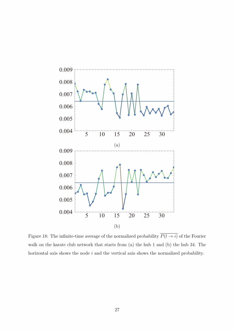
Figure 18 (a)–(b) shows the time average of the normalized probabilities of Fourier

walks which start from the hubs (the nodes 1 and 34). We again define the threshold to

be 1/D, where D = 156. The nodes whose probabilities are higher than the threshold

belong to the community in which the initial node is the hub. For instance, if the Fourier

walk starts from the hub 1, the probability of the node 2, which belongs to the same

community, is higher than the threshold. We can thus detect which community each

node belongs to.

A comment is in order here; the detection of the nodes 3 and 20 are quite marginal

although correct. There are indeed several views of the grouping of several nodes. One

research [41] divided the nodes into three groups. The first partition is the group of the

node 1, the second is the group of the node 34, and the third is a neutral group, whose

nodes are 9, 10, 20, 28, 29. It is therefore reasonable that the node 20 has a marginal

value in Fig. 18 (b). Another research [13] shows that their algorithm classified the node 3

23

1 5 10 15 211

5

10

15

21

0

0.01

0.02

0.03

0.04

0.05

0.06

(a)

1 5 10 15 211

5

10

15

21

0

0.01

0.02

0.03

0.04

0.05

0.06

(b)

1 5 10 15 211

5

10

15

21

0

0.01

0.02

0.03

0.04

0.05

0.06

(c)

1 5 10 15 211

5

10

15

21

0

0.01

0.02

0.03

0.04

0.05

0.06

(d)

1 5 10 15 211

5

10

15

21

0

0.01

0.02

0.03

0.04

0.05

0.06

(e)

1 5 10 15 211

5

10

15

21

0

0.01

0.02

0.03

0.04

0.05

0.06

(f)

1 5 10 15 211

5

10

15

21

0

0.01

0.02

0.03

0.04

0.05

0.06

(g)

1 5 10 15 211

5

10

15

21

0

0.01

0.02

0.03

0.04

0.05

0.06

(h)

1 5 10 15 211

5

10

15

21

0

0.01

0.02

0.03

0.04

0.05

0.06

(i)

Figure 15: The time evolution of the normalized probability Pt(l → i) of the classical

random walk on the three-community network: (a) the zeroth step; (b) the first step; (c)

the second step; (d) the third step; (e) the fourth step; (f) the fifth step; (g) the thirtieth

step; (h) the eighty-fourth step; (i) the hundredth step. The vertical axis shows the initial

node l and the horizontal axis shows the node i. A white square indicates a value off the

scale in the higher direction.

24

2

1 3

4

56

78

9

10

11

12 13

1417

1820

22

26

24

25

28

29 30 27

31

32

33

15

16

19

21

23

34

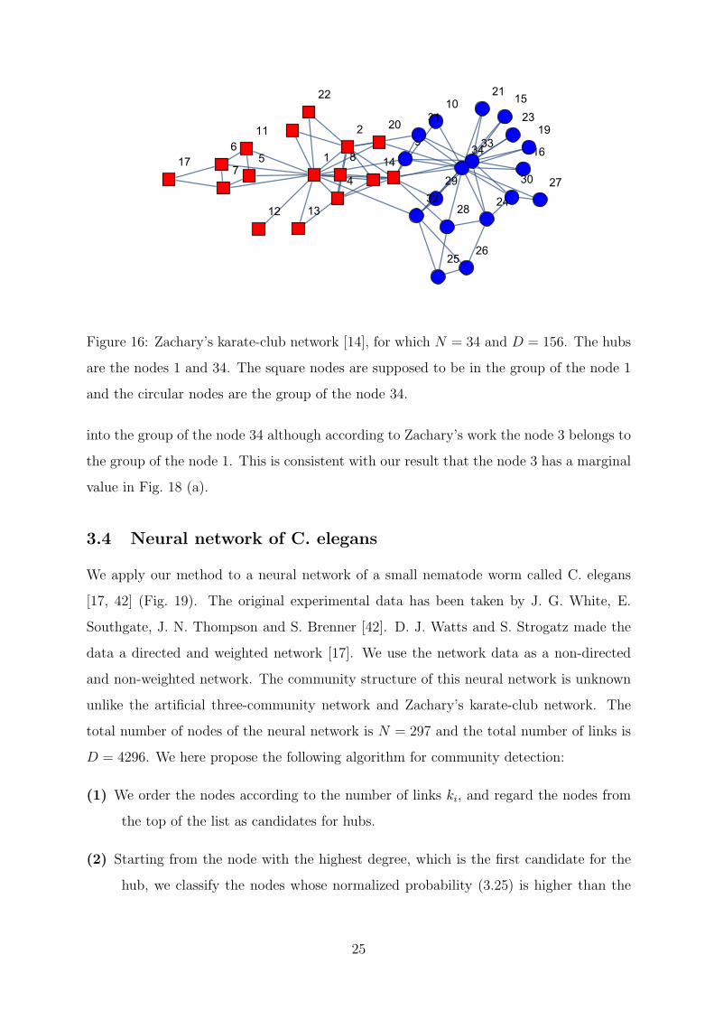
Figure 16: Zachary’s karate-club network [14], for which N = 34 and D = 156. The hubs

are the nodes 1 and 34. The square nodes are supposed to be in the group of the node 1

and the circular nodes are the group of the node 34.

into the group of the node 34 although according to Zachary’s work the node 3 belongs to

the group of the node 1. This is consistent with our result that the node 3 has a marginal

value in Fig. 18 (a).

3.4 Neural network of C. elegans

We apply our method to a neural network of a small nematode worm called C. elegans

[17, 42] (Fig. 19). The original experimental data has been taken by J. G. White, E.

Southgate, J. N. Thompson and S. Brenner [42]. D. J. Watts and S. Strogatz made the

data a directed and weighted network [17]. We use the network data as a non-directed

and non-weighted network. The community structure of this neural network is unknown

unlike the artificial three-community network and Zachary’s karate-club network. The

total number of nodes of the neural network is N = 297 and the total number of links is

D = 4296. We here propose the following algorithm for community detection:

(1) We order the nodes according to the number of links ki, and regard the nodes from

the top of the list as candidates for hubs.

(2) Starting from the node with the highest degree, which is the first candidate for the

hub, we classify the nodes whose normalized probability (3.25) is higher than the

25

1 10 20 341

10

20

34

0

0.025

0.050

0.075

0.100

0.125

0.150

The target node i

The

initi

al n

ode

l

Figure 17: The infinite-time average of the probability p(l → i) of the Fourier walk on

the karate-club network. The vertical axis shows the initial node l and the horizontal axis

shows the target node i.

threshold 1/D into the community of the hub.

(3) We carry out (2) repeatedly, ignoring the nodes that have been classified, till all of

the nodes are classified into any community. If the node with the highest degree

at the moment (e.g. the node 2 in Fig. 20) has been already classified into any

community (e.g. the green broken circle in Fig. 20), we assume that the hub and

the nodes which are the members of the group of the hub (e.g. the red broken circle

in Fig. 20), belong to the community into which the hub has been classified (e.g. the

solid circle in Fig. 20).

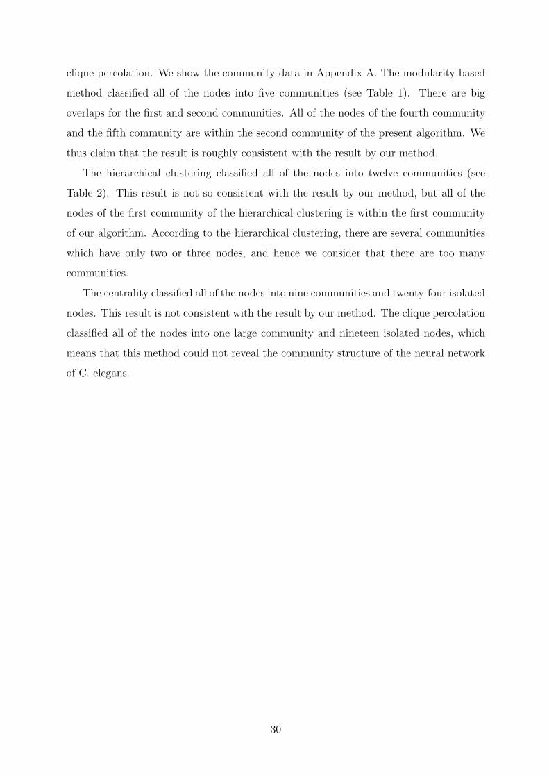
Figure 21 shows the result of the community detection for the neural network. We clas-

sified all of the nodes into three communities.

We compared our result to those by other methods: the hierarchical clustering, the

modularity-based method, the centrality and the clique percolation. These methods are

implemented in Mathematica under the command named FindGraphCommunities, al-

though we do not know what specific algorithms Mathematica utilizes; the standard

references are, for example, Refs. [23, 26] for the hierarchical clustering, Refs. [23, 28] for

the modularity-based method, Refs. [43, 44] for the centrality and Refs. [23, 45] for the

26

5 10 15 20 25 300.004

0.005

0.006

0.007

0.008

0.009

(a)

5 10 15 20 25 300.004

0.005

0.006

0.007

0.008

0.009

(b)

Figure 18: The infinite-time average of the normalized probability P (l → i) of the Fourier

walk on the karate club network that starts from (a) the hub 1 and (b) the hub 34. The

horizontal axis shows the node i and the vertical axis shows the normalized probability.

27

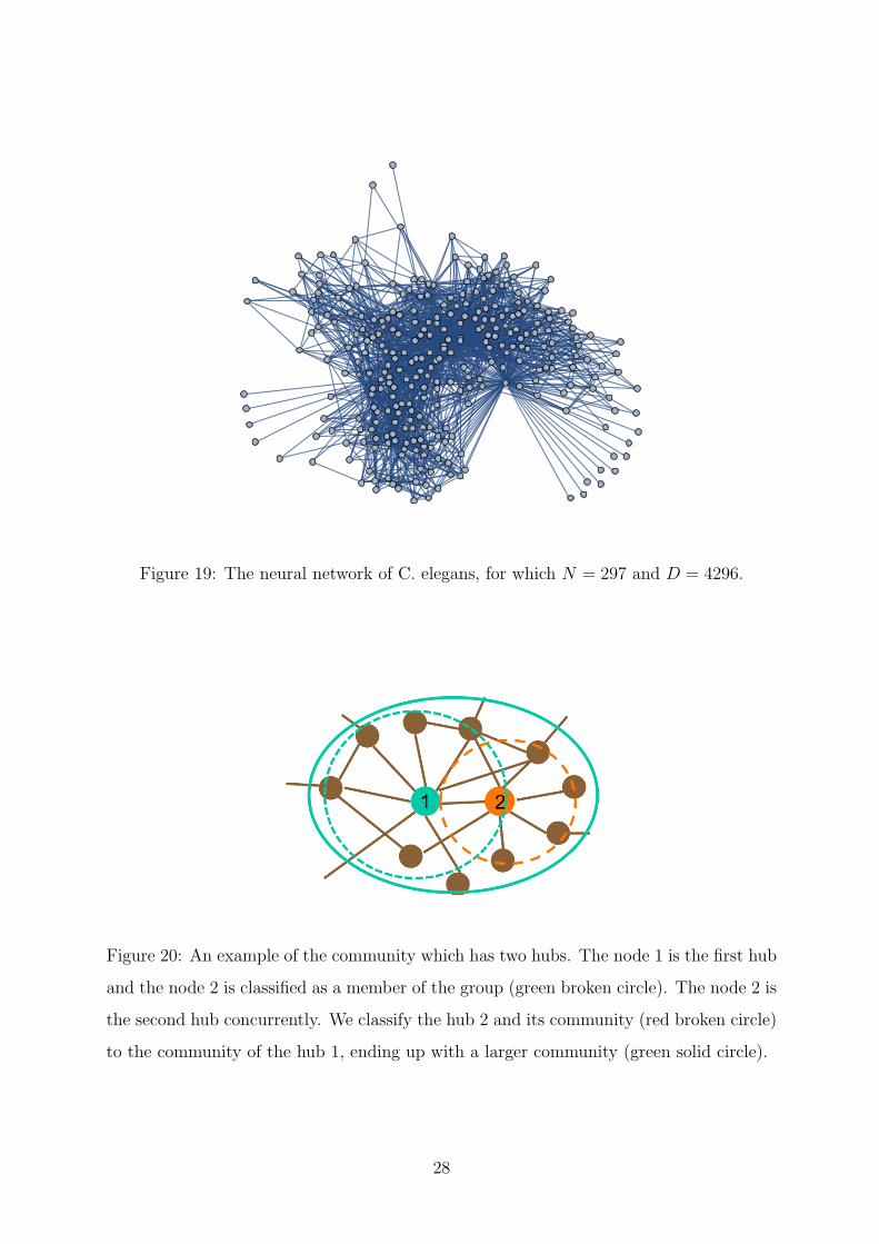
Figure 19: The neural network of C. elegans, for which N = 297 and D = 4296.

Figure 20: An example of the community which has two hubs. The node 1 is the first hub

and the node 2 is classified as a member of the group (green broken circle). The node 2 is

the second hub concurrently. We classify the hub 2 and its community (red broken circle)

to the community of the hub 1, ending up with a larger community (green solid circle).

28

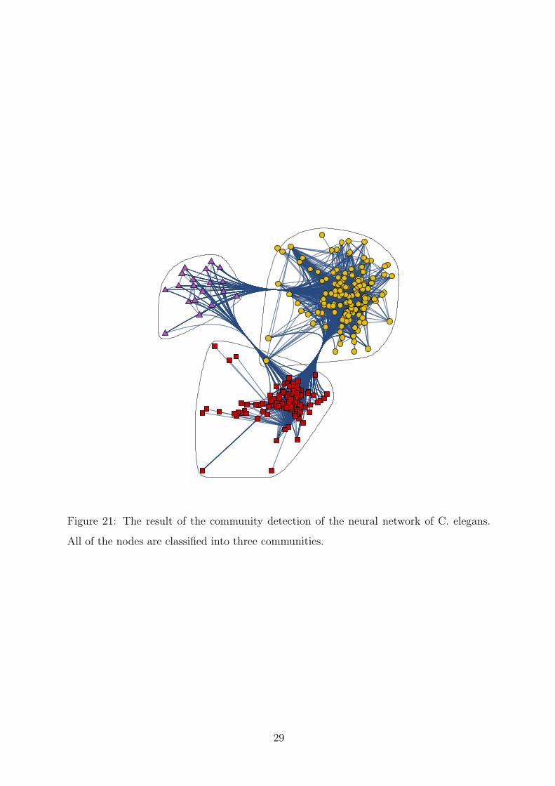
Figure 21: The result of the community detection of the neural network of C. elegans.

All of the nodes are classified into three communities.

29

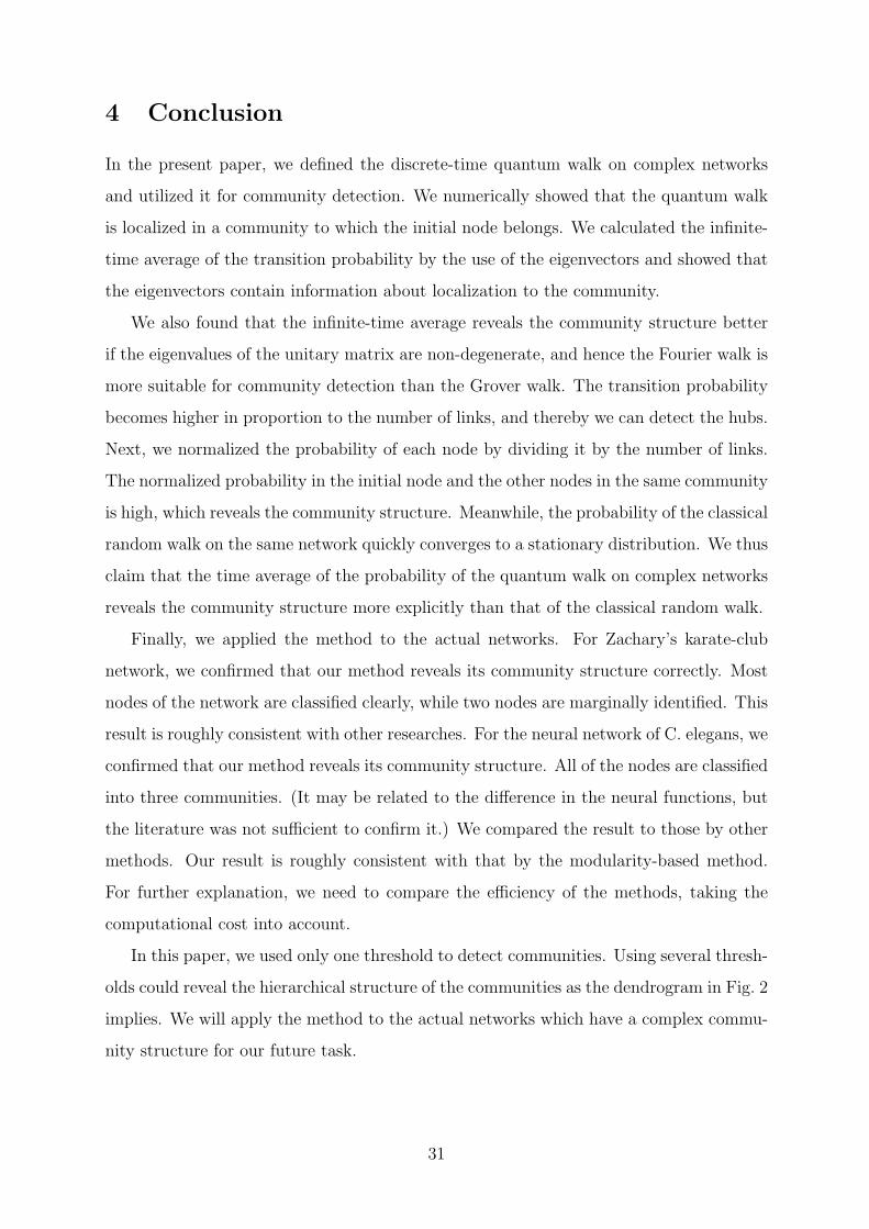
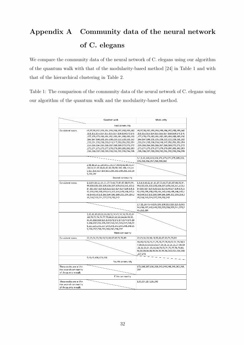
clique percolation. We show the community data in Appendix A. The modularity-based

method classified all of the nodes into five communities (see Table 1). There are big

overlaps for the first and second communities. All of the nodes of the fourth community

and the fifth community are within the second community of the present algorithm. We

thus claim that the result is roughly consistent with the result by our method.

The hierarchical clustering classified all of the nodes into twelve communities (see

Table 2). This result is not so consistent with the result by our method, but all of the

nodes of the first community of the hierarchical clustering is within the first community

of our algorithm. According to the hierarchical clustering, there are several communities

which have only two or three nodes, and hence we consider that there are too many

communities.

The centrality classified all of the nodes into nine communities and twenty-four isolated

nodes. This result is not consistent with the result by our method. The clique percolation

classified all of the nodes into one large community and nineteen isolated nodes, which

means that this method could not reveal the community structure of the neural network

of C. elegans.

30

4 Conclusion

In the present paper, we defined the discrete-time quantum walk on complex networks

and utilized it for community detection. We numerically showed that the quantum walk

is localized in a community to which the initial node belongs. We calculated the infinite-

time average of the transition probability by the use of the eigenvectors and showed that

the eigenvectors contain information about localization to the community.

We also found that the infinite-time average reveals the community structure better

if the eigenvalues of the unitary matrix are non-degenerate, and hence the Fourier walk is

more suitable for community detection than the Grover walk. The transition probability

becomes higher in proportion to the number of links, and thereby we can detect the hubs.

Next, we normalized the probability of each node by dividing it by the number of links.

The normalized probability in the initial node and the other nodes in the same community

is high, which reveals the community structure. Meanwhile, the probability of the classical

random walk on the same network quickly converges to a stationary distribution. We thus

claim that the time average of the probability of the quantum walk on complex networks

reveals the community structure more explicitly than that of the classical random walk.

Finally, we applied the method to the actual networks. For Zachary’s karate-club

network, we confirmed that our method reveals its community structure correctly. Most

nodes of the network are classified clearly, while two nodes are marginally identified. This

result is roughly consistent with other researches. For the neural network of C. elegans, we

confirmed that our method reveals its community structure. All of the nodes are classified

into three communities. (It may be related to the difference in the neural functions, but

the literature was not sufficient to confirm it.) We compared the result to those by other

methods. Our result is roughly consistent with that by the modularity-based method.

For further explanation, we need to compare the efficiency of the methods, taking the

computational cost into account.

In this paper, we used only one threshold to detect communities. Using several thresh-

olds could reveal the hierarchical structure of the communities as the dendrogram in Fig. 2

implies. We will apply the method to the actual networks which have a complex commu-

nity structure for our future task.

31

Appendix A Community data of the neural network

of C. elegans

We compare the community data of the neural network of C. elegans using our algorithm

of the quantum walk with that of the modularity-based method [24] in Table 1 and with

that of the hierarchical clustering in Table 2.

Table 1: The comparison of the community data of the neural network of C. elegans using

our algorithm of the quantum walk and the modularity-based method.

32

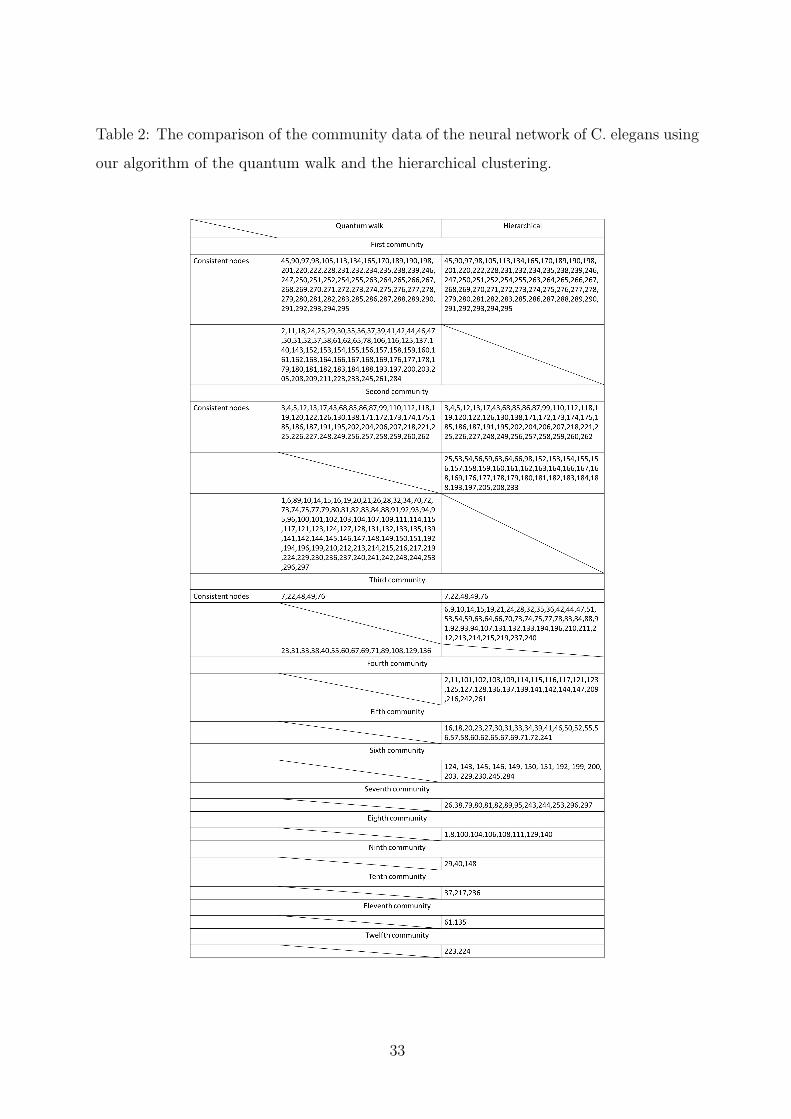
Table 2: The comparison of the community data of the neural network of C. elegans using

our algorithm of the quantum walk and the hierarchical clustering.

33

References

[1] Y. Aharonov, L. Davidovich, and N. Zagury, Quantum random walks, Phys. Rev. A

48, 1687 (1993)

[2] E. Farhi and S. Gutmann, Quantum computation and decision trees, Phy. Rev. A

58, 915 (1998)

[3] D. Aharonov, A. Ambainis, J. Kempe, and U. V. Vazirani, Quantum walks on graphs,

Proc. of the 33rd Annual ACM Symposium on Theory of Computing, 50–59, quant-

ph/0012090 (2001)

[4] N. Inui, N. Konnno, and E. Segawa, One-dimensional three-state quantum walk,

Phys. Rev. E 72, 056112 (2005)

[5] T. Machida, Limit theorems for a localization model of 2-state quantum walk, Int.

J. Quant. Inf., 9, 863–874 (2011)

[6] A. C. Oliveira, R. Portugal and R. Donangelo, Decoherence in two-dimensional quan-

tum walks, Phys. Rev. A 74, 012312 (2006)

[7] K. Sato, Periodicity for the Fourier quantum walk on regular graphs,

arXiv:1811.03235v1 (2018)

[8] L. Grover, A fast quantum mechanical algorithm for database search, Proc. of the

28th Annual ACM Symposium on Theory of Computing, 212–219 (1996)

[9] S. D. Berry, and B. J. Wang, Quantum-walk-based search and centrality, Phys. Rev.

A 82, 042333 (2010)

[10] B. C. Travaglione and G. J. Milburn, Implementing the quantum random walk, Phys.

Rev. A 65, 032310 (2002)

[11] A. Crespi, R. Osellame, R. Ramponi, M. Bentivegna, F. Flamini, N. Spagnolo, N.

Viggianiello, L. Innocenti, P. Mataloni and F. Sciarrino, Suppression law of quantum

states in a 3D photonic fast Fourier transform chip, Nat. Commun. 7, 10469 (2016)

34

[12] A. Montanaro, Quantum walks on directed graphs, Quantum Information and Com-

putation 7 (1-2), 93–102 (2007)

[13] M. Girvan and M. E. J. Newman, Community structure in social and biological

networks. Proc. Natl. Acad. Sci. USA 99, 7821–7826 (2002)

[14] W. W. Zachary, An Information Flow Model for Conflict and Fission in Small Groups,

J. Anthropol. Res. 33, 452–437 (1977)

[15] G. W. Flake, S. Lawrence, C. Lee Giles, F. M. Coetzee, Self-organization and iden-

tification of web communities, IEEE Computer 35, 66–71 (2002)

[16] M. Takayasu, S. Sameshima, T. Ohnishi, Y. Ikeda, H. Takayasu and K. Watanabe,

Massive economics data analysis by econophysics methods - the case of companies’

network structure, Annual Report of the Earth Simulator Center April 2007–March

2008, pp. 263–268 (2008)

[17] D. J. Watts and S. H. Strogatz, Collective dynamics of ’small-world’ networks, Nature

(London) 393, 440–442 (1998)

[18] R. J. Williams and N. D. Martinez, Simple rules yield complex food webs, Nature

(London) 404, 180–183 (2000)

[19] A. W. Rives, T. Galitski, Modular organization of cellular networks, Proc. Natl.

Acad. Sci. USA 100 (3), 1128–1133 (2003)

[20] F. Radicchi, C. Castellano, F. Cecconi, V. Loreto, and D. Parisi., Defining and

identifying communities in networks, Proc. Natl. Acad. Sci. U. S. A., 101 (9), 2658–

2663 (2004)

[21] S. H. Strogatz, Exploring complex networks, Nature (London) 410, 268–276 (2001)

[22] S. Milgram, The Small World Problem, Psycohology Today, 1 (1), 61–67 (1967)

[23] S. Fortunato, Community detection in graphs, Phys. Rep. 486, 75–174 (2010)

[24] M. E. J. Newman, Finding community structure in networks using the eigenvectors

of matrices, Phys. Rev. E 74 (3), 036104 (2006)

35

[25] P. Pons and M. Latapy, Computing communities in large networks using random

walks, Springer, New York, 284–293 (2005)

[26] T. Hastie, R. Tibshirani and J. H. Friedman, The Elements of Statistical Learning,

Springer Berlin Germany, ISBN 0387952845 (2001)

[27] E. Estrada and N. Hatano, Communicability in complex networks, Phys. Rev. E 77,

036111 (2008)

[28] M. E. J. Newman, Modularity and community structure in networks, Proc. Natl.

Acad. Sci. USA 103, 8577-8582 (2006)

[29] A. Clauset, M. E. J. Newman, and C. Moore, Finding community structure in very

large networks, Phys. Rev. E 70, 066111 (2004)

[30] M. Rosvall, and C. T. Bergstrom, Maps of random walks on complex networks reveal

community structure. Proc. Natl Acad. Sci. USA 105, 1118–1123 (2008)

[31] A. M. C. Souza, and R. F. S. Andrade, Discrete time quantum walk on the Apollonian

network, J. Phys. A: Math. Theor. 46, 145102 (2013)

[32] N. Shenvi, J. Kempe, and K. B. Whaley, Quantum random-walk search algorithm,

Phys. Rev. A 67, 052307 (2003)

[33] Y. Higuchi, N. Konno, I. Sato, and E. Sagawa, Periodicity of the discrete-time quan-

tum walk on a finite graph, Interdiscip. Inf. Sci., 23, 75–86 (2017)

[34] Y. Ide, N. Konno, and E. Segawa, Time averaged distribution of a discrete-time

quantum walk on the path, Quantum Inf. Process. 11, 1207–1218 (2012)

[35] P. Pradhan, A. Yadav, S. K. Dwivedi, and S. Jalan, Optimized evolution of networks

for proncipal eigenvector localization, Phys. Rev. E 96, 022312 (2017)

[36] A. V. Goltsev, S. N. Dorogovtsev, J. G. Oliveira, and J. F. F. Mendes, Localization

and Spreading of Diseases in Complex Networks, Phys. Rev. Lett. 109, 128702 (2012)

[37] P. W. Anderson, Absence of Diffusion in Certain Random Lattices, Phys. Rev. 109,

1492 (1958)

36

[38] T. Devakul and D. A. Huse, Anderson localization transitions with and without

random potentials, Phys. Rev. B 96, 214201 (2017)

[39] I. Vakulchyk, M. V. Fistul, P. Qin, and S. Flach, Anderson localization in generalized

discrete time quantum walks, Phys. Rev. B 96, 144204 (2017)

[40] S. Derevyanko, Anserson localization of a one-dimensional quantum walker, Scientific

Reports 8 (1), 1795 (2018)

[41] H. Wu, L. Gao, J. Dong, and X. Jang, Detecting overlapping protein complexes by

rough-fuzzy clustering in protein-protein networks, Pros ONE 9 (3), e91856 (2014)

[42] J. G. White, E. Southgate, J. N. Thomson and S. Brenner, The structure of the

nervous system of the nematode Caenorhabditis elegans, Phil. Trans. R. Soc. London

314, 1–340 (1986)

[43] A. Bavelas, A mathematical model for group structures, Human organization 7 (3),

16–30 (1948)

[44] R. K. Behera, D. Naik, B. Sahoo and S. Ku. Rath, Centrality approach for commu-

nity detection in large scale network, in Proceedings of the 9th Annual ACM India

Conference, pp. 115–124 (ACM, New York, 2016)

[45] I. Derenyi, G. Palla and T. Vicsek, Clique Percolation in Random Networks, Phys.

Rev. Lett, 94 160202 (2005)

37