Embed Size (px)
Citation preview

MASTER THESIS- Towards Automated Fault Management in Smart Grid
Communication Networks -
Master thesis
DOUMERC ROBIN
MSc. Networks and Distributed SystemsDepartment of Electronic Systems
Fredrik Bajers Vej 7BDK-9220 Aalborg

“Dans les champs de l’observation le hasard ne favorise que les esprits préparés”“Where observation is concerned, chance favours only the prepared mind”
Louis Pasteur

Department of Electronic SystemsFredrik Bajers Vej 7DK-9220 Aalborg Ø
http://es.aau.dk
Title:Towards Automated Fault Managementin Smart Grid Communication Networks.
Theme:Smart Grid, Fault Detection, NetworkMonitoring
Project Period:September 2013-June 2014
Project Group:1027
Participant(s):Doumerc Robin
Supervisor(s):Jose Manuel Gutierrez LopezRasmus Løvenstein Olsen
Copies: 4
Page Numbers: ??
Date of Completion:June 4, 2014
Abstract:
This master thesis deals with auto-mated fault management in communi-cation systems, with a particular inter-est on smart grid networks.Smart grid is the upcoming way to man-age the electricity grid, using moderncommunication technics and a decen-tralized architecture.Due to the criticality of the data, smartgrid systems use a two-networks solu-tion, one primary and a backup one.Such configuration has been emulatedin the simulator OMNeT++, usingADSL and LTE as a first and secondarynetwork.A fault detection algorithm based onprobe’s metrics such as end-to-end de-lay and inter-arrival time of probes,has been implemented. The results ofthe simulations show that the detectionprocess is functional. However, the bestperformances are obtained using high-frequency probes, which can reduce thescalability of such systems.some future works could focus on theuse of other principal networks such asWireless Mesh, or simulations workingon test beds.
The content of this report is freely available, but publication (with reference) may only be pursueddue to agreement with the author.


Acknowledgements
I wish to thanks my supervisors Jose Manuel Gutierrez Lopez & Rasmus LøvensteinOlsen for their precious advices and their guidance all along this year regarding thisthesis.
I would like to thanks the Aalborg University for the quality of the educationhere and to have given me the chance to stay after my Erasmus year in order tocomplete this MSc .
I would also thanks my French school of engineering, the Ecole Superieure d’Ingenieuren Electronique et Electrotechnique, that allowed me to take a sabbatical in orderto stay in Denmark one more year.
Finally, I would like to express my gratitude to my parents. Their support andaffection throughout my years of studies was invaluable. Their package of Frenchfood during the year strongly helped me support the scandinavian winter.
v


Contents
Preface xi
Reading Guide xiii
1 Introduction 11.1 Historical Overview . . . . . . . . . . . . . . . . . . . . . . . . . . . . . 21.2 Smart Grid Power components . . . . . . . . . . . . . . . . . . . . . . 31.3 Motivation . . . . . . . . . . . . . . . . . . . . . . . . . . . . . . . . . 71.4 Problem Formulation . . . . . . . . . . . . . . . . . . . . . . . . . . . . 8
2 Smart Grid Communication Systems and Applications 112.1 Network architecture . . . . . . . . . . . . . . . . . . . . . . . . . . . . 11
2.1.1 Customer premise . . . . . . . . . . . . . . . . . . . . . . . . . 122.1.2 Last Mile . . . . . . . . . . . . . . . . . . . . . . . . . . . . . . 122.1.3 Back-haul . . . . . . . . . . . . . . . . . . . . . . . . . . . . . . 122.1.4 Wide Area Network . . . . . . . . . . . . . . . . . . . . . . . . 12
2.2 Smart Grid communication technologies . . . . . . . . . . . . . . . . . 122.2.1 IEEE 802.15.4 (Zigbee & 6loWPAN) . . . . . . . . . . . . . . . 132.2.2 Wireless Mesh Networks . . . . . . . . . . . . . . . . . . . . . . 142.2.3 WiMAX . . . . . . . . . . . . . . . . . . . . . . . . . . . . . . . 142.2.4 Cellular Networks . . . . . . . . . . . . . . . . . . . . . . . . . 152.2.5 Digital Subscriber Lines . . . . . . . . . . . . . . . . . . . . . . 162.2.6 Power Line Communication . . . . . . . . . . . . . . . . . . . . 162.2.7 FTTx . . . . . . . . . . . . . . . . . . . . . . . . . . . . . . . . 162.2.8 Choice for simulation . . . . . . . . . . . . . . . . . . . . . . . 17
2.3 Applications and requirements . . . . . . . . . . . . . . . . . . . . . . 20
3 Network performance and Monitoring 233.1 Systems and Faults . . . . . . . . . . . . . . . . . . . . . . . . . . . . . 23
3.1.1 System components & Failure probability . . . . . . . . . . . . 233.1.2 Dependability of the system . . . . . . . . . . . . . . . . . . . . 243.1.3 Concept of Fault Management . . . . . . . . . . . . . . . . . . 26
3.2 Anomalies in the network traffic . . . . . . . . . . . . . . . . . . . . . 27
vii

viii Contents
3.3 Monitoring and Fault detection . . . . . . . . . . . . . . . . . . . . . . 293.3.1 Choice for the simulation . . . . . . . . . . . . . . . . . . . . . 32
4 Simulation Model 334.1 Networks description . . . . . . . . . . . . . . . . . . . . . . . . . . . . 334.2 Simulator description . . . . . . . . . . . . . . . . . . . . . . . . . . . . 35
4.2.1 OMNeT++ . . . . . . . . . . . . . . . . . . . . . . . . . . . . . 354.2.2 INET . . . . . . . . . . . . . . . . . . . . . . . . . . . . . . . . 374.2.3 SIMULTE . . . . . . . . . . . . . . . . . . . . . . . . . . . . . . 37
4.3 Network description in OMNeT++ . . . . . . . . . . . . . . . . . . . . 384.3.1 IP Adress attribution . . . . . . . . . . . . . . . . . . . . . . . 384.3.2 LTE BINDER . . . . . . . . . . . . . . . . . . . . . . . . . . . 404.3.3 Channel Controler . . . . . . . . . . . . . . . . . . . . . . . . . 404.3.4 Hosts . . . . . . . . . . . . . . . . . . . . . . . . . . . . . . . . 414.3.5 Internet Core Network . . . . . . . . . . . . . . . . . . . . . . . 424.3.6 Scenario Management . . . . . . . . . . . . . . . . . . . . . . . 43
4.4 Internet Traffic Description . . . . . . . . . . . . . . . . . . . . . . . . 444.4.1 Periodicity of the Traffic . . . . . . . . . . . . . . . . . . . . . . 444.4.2 Delay characterisation . . . . . . . . . . . . . . . . . . . . . . . 444.4.3 Queue description . . . . . . . . . . . . . . . . . . . . . . . . . 45
4.5 Faults detection Algorithms . . . . . . . . . . . . . . . . . . . . . . . . 474.5.1 Fault detection - House’s Point of view . . . . . . . . . . . . . . 484.5.2 Fault detection - Aggregator’s Point of view . . . . . . . . . . . 51
4.6 OMNeT++ Implementation . . . . . . . . . . . . . . . . . . . . . . . . 554.7 Data collection- Signal mechanism . . . . . . . . . . . . . . . . . . . . 57
5 Results 595.1 Parameters and variables . . . . . . . . . . . . . . . . . . . . . . . . . 59
5.1.1 Random Number Generation . . . . . . . . . . . . . . . . . . . 595.1.2 Simulation parameters . . . . . . . . . . . . . . . . . . . . . . . 605.1.3 Simulation variables . . . . . . . . . . . . . . . . . . . . . . . . 60
5.2 Fault Detection . . . . . . . . . . . . . . . . . . . . . . . . . . . . . . . 605.2.1 Caracterisation of the Delay and Inter-arrival rate . . . . . . . 605.2.2 Router Shutdown . . . . . . . . . . . . . . . . . . . . . . . . . . 615.2.3 Latency Increase . . . . . . . . . . . . . . . . . . . . . . . . . . 645.2.4 Restauration Process . . . . . . . . . . . . . . . . . . . . . . . . 655.2.5 Effect on the LTE network . . . . . . . . . . . . . . . . . . . . 65
5.3 Discussion . . . . . . . . . . . . . . . . . . . . . . . . . . . . . . . . . . 67
6 Conclusion 69
7 Future Work 71
Bibliography 73

Nomenclature
AMI Advance Metering Infrastructure
DIX Danish Internet Exchange Point
DSLAM Digital Subscriber Line Access Multiplexer
FTTx Fiber To The x
ISP Internet Service Provider
LTE Long Term Evolution
M2M Machine to Machine
NED Network Description
PGW Public Data Network Gateway
PLC Power Line Communication
PMU Phasor Measurement Unit
PRNG Pseudo Random Number Generation
QOS Quality of Service
SCADA Supervisory Control And Data Acquisition
SGW Service Gateway
SG Smart Grid
UE User Equipment
WAN Wide Area Network
WMN Wireless Mesh Network
xDSL Digital Suscriber Line
ix

x Contents

Preface
This thesis concludes my Master of Science education in the field of Networks andDistributed systems at Aalborg University. The thesis was performed throughoutmy 9th and 10th semester, year 2013/2014, at the Department of Electronics.the thesis deals with the study automated fault management in smart grid commu-nication systems.Citations will be shown as the number of a specific reference within brackets likethis: [1] which will link to the source list at the end of the report.Simulation data are obtained using the network simulator OMNeT++. It is assumedthat the reader may not be familiar with it and therefore, the way the simulator op-erates is detailed in chapter 4.All schematics or flowcharts are obtained using Microsoft Visio, while the plots arefrom Matlab.
Aalborg University, June 4, 2014
DOUMERC ROBIN<[email protected]>
xi

xii Contents

Reading guide
The sections described are referred as (number of section). The Chapter 1 containsan introduction regarding the current electric grid, and why the smart grid is needed.At the end of this introduction is stated the motivation of the thesis, and a problemis formulated.
The first part of Chapter 2 describes the different tiers composing the com-munication systems of smart grids (2.1). It is followed by an overview of differenttechnologies (2.2) that can be used at every level of the network. Finally, the lastsection highlights the various applications that can be used in smart grid systems,among with the quality of service requirements (2.3).
The Chapter 3 focuses on the dependability of a system. The initial part de-fines the attributes of a dependable system, and the different steps of fault manage-ment(3.1). The second part defines the anomalies a network can encounter (3.2),while the last one is narrowed down to the detection process, and how faults can bedetected in a communication network (3.3).
The Chapter 4 is about the model used during the simulation. The first sectiondescribe the network architecture used (section 4.2). It is followed by the descrip-tion of OMNeT++, from the general functioning (4.1), to the specific modules usedfor the experiments (4.3). The section 4.5 describes the algorithm designed for thethesis, while section 4.6 focuses on the implementation in the simulator.
Finally, Chapter 5 will be used to discuss the results of the experiments, whileChapter 6 and Chapter 7 will conclude and open the path to future work.
xiii

xiv Contents

Chapter 1
Introduction
NB: Part of this introduction has been written in collaboration with group 921 (Mo-hammed Seifu Kemal and Alexandru Ceocea) during the Autumn semester 2013.It istherefore normal that an important number of paragraphs in this introduction may beexactly the same as in their report : "Integration of General Fixed Tele-Infrastructurein Smart Grid Communication Systems"
We use energy, and lots of it. However there are going to be some big changes inthe way we use it. The world is running out of oil and natural gas. Denmark has thevision of becoming politically independent of fossil fuels and so, the energy systemswill be transformed in the years to come.
In the near future, energy will be produced, transported and used in a verydifferent and far more efficient manner than that the one for which the power systemwas originally designed.
Until recently, electricity was produced in large central coal plants close to thecities and industrial areas, and then transported on to the consumers. Althoughthis has already changed, when thousands of new wind turbines, photovoltaic plantsand heat pumps have appeared all around Denmark. Simply put, energy today isproduced everywhere and it is transported in all directions in the power system. Thistrend will most certainly intensify in the future.
The houses and commercial buildings in the future will be intelligent, which meansthat automated intelligent systems will control the energy consumption. A/C units,freezers, refrigeration units, heat pumps and other appliances will all be controlledin such a way as to increase efficiency and decrease costs.
In the coming years, electricity production and consumption will change consid-erably. Energy generation will be based more on renewable energy sources and lessof fossil fuels and consumers will change the way they use this energy.
In the traditional sense of a power grid, the consumers (household and commer-cial consumers) have mostly been passive components, with predictable and regularconsumption patterns. [1]
In an intelligent power system, namely a Smart Grid, new opportunities and
1

2 Chapter 1. Introduction
perspectives emerge. Such as the ability for the consumers to interact with the powersystem and generate energy which can be distributed in the grid, thus becomingresources.
1.1 Historical OverviewDifferent studies show that there is a causality between the increase of the Gross
Domestic Product, and the consumption of energy and particularly electricity [2].After World War II, and especially with the reconstruction of Europe, most of thedeveloped countries acknowledged a strong growth until the first oil chock in 1973.This period also created a lot of knew habits for people, bringing inside homes alot of brand new electrical objects to make their lives easier. These new needs inelectricity lead the different states to design and build a powerful and broad electricgrid, in order to supply the demand. Although, the needs of electricity growthover the years (the consumption of electricity in the world was doubled since 1965[3], but the grid has almost not changed since 1960’s. This is explained by the longprocedures, time and money consuming plans in order to build high voltage overheadpower line, and sometimes the opposition of the population leaving nearby. So, thecurrent grid is ancient, and the current consumption is higher than for what it hasbeen designed. Moreover, this grid has been designed by each state on a countryscale, with some interconnection between other countries in order to provide somemutual assistance. Nevertheless, from the past decade, this approach is no longervalid, and the cross country connections are used to shift growing power volumesover the whole continent.
Furthermore, the grid has been designed according to a vertical service: a powerplant produces the electricity, and it is delivered through the grid.Those power plantswere rare and placed at some strategic point(close to primary resources) and weredesigned to produce a large amount of electricity and be able to provide for thewhole grid. Yet, with the implementation of renewable energy sources, such aswindmills or solar panels, the production of energy is more distributed all over thegrid. Beside, the production of energy is also random: indeed, renewable energiesare more subject to external factors (wind, sun, etc.) than traditional power plantssuch as nuclear or charcoal are. The main consequence to that is the load on thepower lines is very variable, but the absence of proper sensors & a communicationnetwork that belongs with the electric grid, in order to control the grid, implies thatthe regulation has to be human based. And despite an already existent coordinationthroughout the different actors of the grid, the high power volumes over the gridplus the instability of the grid which is not designed for the current need, and alsothe lack of automated regulation can lead to major failure in the system. This wasthe case, for example, in November 2006, where a planned power cut in NorthernGermany introduced a blackout for more than 15 Millions people for 40 minutes,and introduced disturbances in all electric lines (e.g frequency shift) in Europe fora bit less than two hours[4]. To avoid these kinds of major failures, smart grids are

1.2. Smart Grid Power components 3
needed.
1.2 Smart Grid Power componentsA power system may be viewed as a network of Electrical Systems working to-
gether for Generating, Transmitting and usage of Electrical Energy. This system isresponsible for supplying Electric power to homes, industries, business, schools andvarious application areas. A modern power system can be viewed as a system withmultiple main components:
• Power Plant
• Transmission lines
• Substations
• Distribution lines
• Transformers
• Distribution Substations
• Distributed Energy storage

4 Chapter 1. Introduction
Figure 1.1: Electricity grid schematic and components

1.2. Smart Grid Power components 5
Power Plant - A power generating plant is an industry which generates electricalpower by means of conversion from mechanical energy to electrical energy. The maincomponent of this major subsystem is the electric generator, which converts thismechanical power to electrical power through a rotating motion between an electricconductor and magnetic field. Electrical Energy sources can be broadly categorizedas Renewable energy sources and non-renewable energy sources.
Non-Renewable Energy - Electricity that is produced at an electric powerplant by using fuel sources such as coal, oil, natural gas, or nuclear energy producesheat energy. This heat energy is used to boil water which changes its state to steam.The high pressure created by the steam spins a turbine which interacts with theelectric conductor and magnetic field to produce electricity. Another non-renewablesource is Uranium. By splitting the atoms through nuclear fission, heat energy iscreated and used for producing Electric energy.
Renewable Energy Sources - Renewable energy sources can be categorized asfollows:
• Solar Energy, which can be turned into electricity and heat;
• Wind Energy - use wind turbines to create mechanical motion;
• Geothermal Energy - use the heat inside Earth’s crust;
• Biomass - plants, firewood, ethanol obtained from corn, bio-diesel;
• Hydro-power - Hydro turbines in hydroelectric generation plants.
The Danish government has set a target which states that 50% of the electricityconsumption should be supplied by wind power by 2020. As shown on the chartbelow, the major sources for electric power now, are non-renewable energy generationplants that use coal. The aim by 2020 is for renewable wind energy to be the dominantsource of electric generation.
Transmission line - Electric power transmission is concerned with transmittingthe generated Electrical energy from distributed renewable or non-renewable plantsto areas where demand centers are located. In practice, transmission lines operateunder circumstances where each are connected to other transmission lines creating Anetwork of transmission lines (a transmission network). The term Grid is used to de-scribe transmission lines, Together with substations and electric power distributions.The voltage levels reach as high as 500kv.

6 Chapter 1. Introduction
Figure 1.2: Danish Energy generation
Substations - An electrical substation which is familiar sight on highways andcities is responsible for changing high voltage power of the electricity from powerplants and transmission lines to lower voltage. The task of supervision and electric-ity distribution is undertaken here .The other main task of substations is to makesure that the distribution network is working safely and efficiently. Some of Thecomponents found in substations are power transformers, switching devices, Circuitbreakers for cutting power in case of outages. Control devices, protection devicesand other components used for measurement are also part of substation. Power fromGeneration may pass/flow through several substations at different voltage levels.
Transformers - A transformer is basically defined as a static machine used fortransforming the power to the desired level. Electric power is generated in low voltagebecause of its cost effectiveness but to decrease the cost of transmission, we have tostep up the power. For high voltage transmissions, the current reduces significantlycausing a low I2R losses which in-turn requires a low cross-sectional area conductor.Because of this reason, the voltage is stepped up at generation and stepped downfor distribution circuits using transformers. Step up transformers and step downtransformers are used accordingly.
Distribution substations - Distribution substations are type of step downtransformers which are the closest to consumers. Usually distribution substationstransform the electricity of low voltage distribution lines to 220v or 400v which aresupply voltage for homes. They are easily recognized mounted on poles especially in

1.3. Motivation 7
rural areas.
Phasor Measurement Unit - The phasor measurement unit is one of thekeystone of smart grid unit.When old meters were only able to monitor the voltagemagnitude every few seconds, the Phasor Measurement Unit (PMU) can measurethe magnitude but also the phase with high precision at a rate between 20 and 120Hz. All the PMU on the system can be synchronized using a GPS clock system.
In conclusion, the electric grid used nowadays is not as hierachical as it wasbefore, but geographycally distributed over diver components. In order to managethis grid, it is then primordial to have measurement everywhere over the grid in orderto be able to monitor the state of the grid.
1.3 MotivationThe Smart Grid concept has been used widely in the recent years in different
contexts and with different definitions. [1]In this thesis, we treat the Smart Grid as a network between the consumers, power
generators and also the equipment necessary to establish and ensure this connection.The future of energy systems will be highly dependable on power systems that
rely on a variety of new electricity generation sources with added consumption mech-anisms. This will drive an Electrical Power System to be flexible and be able tointegrate a very high level of alternative energy sources. A Smart Grid will enablethe power system to collect, exchange and take action to ensure that the reliability,security and efficiency coefficients are maximized and to ensure sustainability of thesystem and the services it provides. [5]
Given the rising demand for energy and also its effect on the cost of electric power,energy companies are competing to take advantage of the new opportunities and tocope with the situation. It is thus, desirable to balance the supply and demand withadditional alternative energy sources and with smarter ways of using the generatedpower. In this case, Wind and Solar Energy play an important role as alternativeenergy resources and need efficient mechanisms to integrate them in the existingpower grid. Although there is a very high demand for the deployment of SmartGrids, their costs and complexity are hindering the faster growth of this technologyaround the globe, but some countries like Denmark and the United Kingdom, aremandating plans for the deployment. In 2011, the smart grid network set up bythe Danish Ministry for Climate and Energy, published a report that points to 35recommendations which contribute to establish a Smart Grid in Denmark. [6]
Smart Grid components, by nature, are spread over different geographical loca-tions, with the generation points and consumption locations being spread almosteverywhere, it is obvious that there is a need for a proper management of locationintelligence. Location intelligence provides information that is essential for smart, ef-ficient and self-healing systems. For the upper management, it provides informationwhich is used for making strategic decisions, mapping of the customers, prospects

8 Chapter 1. Introduction
and suppliers. In the operations part, it provides information regarding differentsmart grid components such as smart meters, aggregators, substations, transformersand alternative energy sources.
st In a smart grid situation, metering systems send data, under certain timeconstraints, to the control centers. Consequently, if the data are not properly sentto those management centers, it is more difficult for the power source companyto regulate the grid. On the electric grid, a small fault can have unpredictablerepercussions on the network leading into a series of other faults, and thus, it iscrucial to be able to detect it quickly in order to prevent a general failure.
In this thesis, my aim is to examine and study the Smart grid communicationinfrastructures, requirements and technologies and use this to design an agent capableof analyzing the dynamics of the network to detect faults and correct them, in orderto maintain all the time a link between each component of the grid.
1.4 Problem FormulationA smart grid network is ubiquitous, with heterogeneous means of communication,and also geographically distributed on a large scale. The organization followed bypower companies is: end-users have smart meters sending data to a control centerDue to the criticallity of metering data, a solution to prevent a breach of communi-cation in case of failure, it is desirable to provide a backup network that will be usedon those case.
To maintain connectivity between these end-users and the management center incase of a failure the link is maintained using an other backup network performing ona different mean of communication.
Figure 1.3: Main and backup network in Smart grid
It is then important for management consideration, to be able to detect anyfailures that are happening in the primary network in order to ensure an interrupted

1.4. Problem Formulation 9
service. Moreover, the handover of many users at the same time, must not impairedthe performance of the backup network and lead to an other failure.This leads to the principal axes that will be followed on this project:
• How to dectect dynamically detect faults on a network using quality of servicemetrics?
• What is the influence of the automated switch of mean of communication onthe network?

10 Chapter 1. Introduction

Chapter 2
Smart Grid CommunicationSystems and Applications
2.1 Network architectureTo understand the stakes of the Smart grid communication network it is im-
portant to detail it architecture, from the end-user to the management and controlcenter.The global communication network in a smart grid is composed of differentheterogeneous tiers of communication networks, the same way the electrical networkis divided in three levels of voltage (High,medium,low).
Figure 2.1: Architecture of Smart Grid Electric and Communication network [7]
The National Institute of Standards, and Technology defines the different tiers of
11

12 Chapter 2. Smart Grid Communication Systems and Applications
the network as follows [8]
2.1.1 Customer premise
This is the customer side of the network. According to the type of customer, threedifferent terms are used: Home Area Network (HAN) for all the network insidehouses with few sensors, Business Area Network (BAN) for buildings with moresensors and Industrial Area Network (IAN) for industries with the higher need involtage. This side of the network can also be connected to auxiliary renewable powersource or electric vehicle. Those networks use smart-meters as gateways to the lastmile network.
2.1.2 Last Mile
This is a two-way communication network that is coupled on top of the power dis-tribution system. According to its characteristics, topology, and service offered,the literature has three terms for the Last Mile access: Neighborhood Area Net-work(NAN),Field Area Networks(FAN) or Advanced metering infrastructure (AMI).This network allows the communication with different renewable-energy generationfarm, connected to the distribution system. This network is also used to make a linkbetween meters in the customer premise, and the data aggregators of the back-haul.
2.1.3 Back-haul
Data from customers’ meters are aggregated at the end of the Last mile Networkthrough aggregators. From there, aggregated data go through a back-haul network,then contains aggregates, but also substations automation parameter’s data, mobileworkforce information from the last mile network. Those data are directed to themajor point of presence of the Wide area network.
2.1.4 Wide Area Network
The Wide Area network (WAN) is composed any different technologies such as fiberoptics, Power Line communication, DSL, and various Wireless communication. Theis designed to support critical application and operation on electric utility infrastruc-ture: relay of High voltage, SCADA, physical security, etc. Typically, the networkis a private network, in order not to rely on public communication due to the criti-cality of the operation, that possess a high-bandwidth backbone/core network Thefollowing section will then present what are the technologies mostly used in order toassure the communication in those unusual tiers.
2.2 Smart Grid communication technologiesIn a Smart Grid network, the importance of real-time and reliable information

2.2. Smart Grid communication technologies 13
becomes paramount and can be considered a key factor in the delivery of power toend-users.[9]. Thus a real-time monitoring is necessary in order to detect any failure.The impact of down-times caused by equipment failures, constraints due to capacityor caused by natural accidents thus becomes much greater than before, but can becontrolled by constant and real-time monitoring.
In the smart grid paradigm, one of the key factor to assure the availability ofthe electric grid, is to have real-time information of the grid using communicationnetworks. It is then primordial to have a reliable communication system coveringthe overall system, in order for the energy companies to have a real-time monitoringof the electricity grid. Any failure on the communication networks can have seriousrepercussion on the overall system.[10]
In a Smart Grid system, data from end-user sensor will go through three differ-ent networks before going to the control center of the energy company. Therefore,multiple technologies,wired or wireless, can be used for Smart Grid networks andthe following sections will be an overview of the pros and cons for the most notabletechnologies that may be used.
2.2.1 IEEE 802.15.4 (Zigbee & 6loWPAN)
The IEEE 802.15.4 is a standard used for Low Rate Wireless Personal AreaNetwork, and specifies the physical layer and the MAC layer. This standard allowsthe uses of a low cost, power efficient and low datarate wireless networks. However,because of the lack of definition of the network layer in IEEE 802.15.4, some other’sstandards on top of it are necessary to build the network.
The Zigbee standard, defined by the Zigbee Alliance, specifies the network layerand also the application one. The standard allows the creation of mesh network,with inherent redundancy, self-configuring, and self-healing capabilities within therange of 10 to 100 meters.[11]
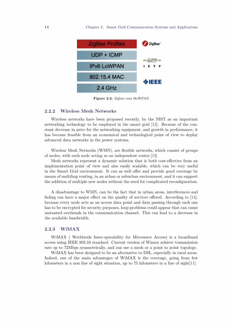
Another standard using as basis the IEEE802.15.4 is the 6loWpan from the In-ternet Engineer Task Force, which allows the use of the IPv6 protocol for low powerprotocols. Because IPv6 requires higher bandwidth than IEEE 802.15.4 can give, the6loWpan protocol reduce the overhead by fragmenting and compressions the head-ers.But, one of the key advantages of the 6loWpan is its complementarily with theZigbee protocol. Indeed, as the figure 2.2 shows, it is possible to use both protocolat the same time, allowing then Zigbee network to have gateways to other Internet-based networks.
However, Zigbee and Zigbee over 6loWPAN have also some disadvantages. Themain one is the uses of the 2.4GHz bands, and therefore, it is subject to interferencefrom other devices using, for example, the IEEE 802.11 (WiFi), or IEEE 802.15(Bluetooth) standards. Furthermore, because of the low-power aspect, the signal issensitive to the environment, especially with concrete walls, reducing considerablythe range of application.
14 Chapter 2. Smart Grid Communication Systems and Applications
Figure 2.2: Zigbee over 6loWPAN
2.2.2 Wireless Mesh Networks
Wireless networks have been proposed recently, by the NIST as an importantnetworking technology to be employed in the smart grid [12]. Because of the con-stant decrease in price for the networking equipment, and growth in performance, ithas become feasible from an economical and technological point of view to deployadvanced data networks in the power systems.
Wireless Mesh Networks (WMN), are flexible networks, which consist of groupsof nodes, with each node acting as an independent router.[13]
Mesh networks represent a dynamic solution that is both cost-effective from animplementation point of view and also easily scalable, which can be very usefulin the Smart Grid environment. It can as well offer and provide good coverage bymeans of multihop routing, in an urban or suburban environment, and it can supportthe addition of multiple new nodes without the need for complicated reconfiguration.
A disadvantage to WMN, can be the fact that in urban areas, interferences andfading can have a major effect on the quality of services offered. According to [14],because every node acts as an access data point and data passing through each onehas to be encrypted for security purposes, loop problems could appear that can causeunwanted overheads in the communication channel. This can lead to a decrease inthe available bandwidth.
2.2.3 WiMAX
WiMAX ( Worldwide Inter-operability for Microwave Access) is a broadbandaccess using IEEE 802.16 standard. Current version of Wimax achieve transmissionrate op to 72Mbps symmetrically, and can use a mesh or a point to point topology.
WiMAX has been designed to be an alternative to DSL, especially in rural areas.Indeed, one of the main advantages of WiMAX is the coverage, going from fewkilometers in a non line of sight situation, up to 75 kilometers in a line of sight[11].

2.2. Smart Grid communication technologies 15
Because Wimax has at been seen only as a wireless DSL alternative, it has beenmainly deployed in rural areas without wire access. However, because of the evolutionof IEEE 802.16, WiMAX offers data transfer speeds close to the LTE standards seenabove, and may be installed more inside cities.
2.2.4 Cellular Networks
Cellular networks are a good option due to the already existent network usedby communication companies. This means that the energy companies can rely onthe existent infrastructure and therefore, will not have to build their own, reducingde facto the time of deployment for the Smart Grid. The different generations forcellular networks will be described.
2G/2.5G
One of the main advantages of the 2G/2.5G is the existing coverage: in Europe,almost 100% of the civilised area are under a 2G/2.5G cell.[11]. It is possible to reacha speed up to 118 kbps in uplink using 2.5G network. However, GSM networks useamong other the 900Mhz band, which penetrates houses but have troubles to reachbasement, where is often located the meters. A solution is to install the antenna abovethe ground level, but this would reduce the cost efficiency of cellular networks uses.2Gtechnology are packed based, low bandwidth, and because it uses IP technology, itsuits for TCP/IP applications where latency and bandwidth are not the main issues.
3G
The 3G and its evolution are perfectly able to provide data services, based on IPand packet oriented, the same way 2G does. It is possible to reach around 14Mbpsin uplink using 3G, up to 23Mbps in 3G+. However, the 3G coverage is inferior to2G, especially in rural area, because of the frequency of 2GHz used in Europe. Nev-ertheless, this may change over the years, due to the reuse from the communicationcompanies of the 900Mhz band used by 2G. This will, de facto, increase the coverage.
LTE
LTE technology is the latest standard used in mobile communication networks. Oneof the main goals of LTE was to reach at least two to three times the 3G+ levelsin uplink (50Mbps). LTE has a high spectral efficiency, a low latency and supportvariable bandwidth. Nonetheless, because the LTE needs a new radio access network,and because it is a recent technology, the actual coverage is limited and concern,mainly big cities.
To sum up, Cellular Networks could be an interesting solution knowing that theenergy companies will use already existing infrastructure, and so reduces the cost ofdeployments. However, to use the network the fees for 3G use can be elevated in thelong term.Also, except for LTE, the latency of cellular is high, which will alter the

16 Chapter 2. Smart Grid Communication Systems and Applications
performance of the network. Moreover, cellular networks are not dedicated, meaningthat all the resources are shared with all the users, leading to a decrease of thenetwork performance. Moreover, if an equipment breakdown appears, a substantialamount of data can be lost, which is not acceptable in case of real-time monitoring.
2.2.5 Digital Subscriber Lines
Digital subscriber Line is a data communications technology allowing fast trans-mission over the telephone network lines. In cities, the use of Very high speed Digitalsubscriber Line can support data rates up to 100 Mbps.
Telephone wire networks are widespread over-all territories, so this solution wouldreduce the implementation cost. However, DSL services can be use just More... onlyover a few kilometers (less than 5km), meaning that this solution would fit purelyfor dense area. Moreover, it is impossible for the end user to split bandwidth witha second modem, meaning that the customer shares the connection with his regularinternet access, to bandwidth issues.
2.2.6 Power Line Communication
Power Line Communication(PLC) is a technique allowing the transmission ofdata using electric power lines. Since most of the devices are already connected tothe power grid, the uses of PLC seem to be a privileged technology. There are noproper open standards for communication over power lines, but most of the time twodifferent approaches are distinguished: the use of narrowband PLC, which perform ona band below 148.5kHz, or the Broadband PLC which is operating between 2-30Mhz.
The obvious advantage of use of PLC in a smart grid system, is that the wirednetwork is already there. However, PLC has also many disadvantages: In orderto make the communication possible, some expensive infrastructures are needed.Moreover, parts of the power in the lines are converted into electromagnetic radiation,leading to a high noise on the medium of transmission. And, PLC is not properlyadapted to a mesh network, including the change of the load over the transmissionline.
2.2.7 FTTx
Optical fiber is currently the fastest medium for data transmission, with a 100 Mbpsin average. Optical fiber is a serious option, due to many advantages: a low latency, ahigh bandwidth, high reliability, a better cost for maintenance than copper. Opticalfiber can be put directly inside the end user house (Fiber To the Home, FTTH), orto a building(Fiber To The Building, FTTB) where another technology (most of thetime, VDSL) ensure the connection.
, However, the fiber network is far from being entirely deployed, and it’s mainly inmajor cities, and the objective in Europe is to have 50 per cent of the population with

2.2. Smart Grid communication technologies 17
fiber access in 2020. So the direct consequences would be the cost of this deployment,around 202 billions to meet the agenda.
The principal attributes of each technologies are summarized in tables 2.1 and2.2.
2.2.8 Choice for simulation
Whatever technology is used as an infrastructure for a smart grid project, each has itsadvantages and disadvantages based on the implementation and application. Whilewired technologies offer good capacity, security and reliability, the costs associatedwith implementation and deployment might favor wireless technologies. Because ofthe geographic distribution, all those technologies may respond to local constraintand therefore be used, leading to a network heterogeneous. However, all the means ofcommunication used must fulfill some traffic requirement according to the applicationthey have been designed for, which will be the topic of the next session.
According to Erhvervsstyrelsen(Danish Business Authority) [15], in 2012, 98% ofthe Danish households are connected to an xDSL connection with at least 2MBpsdata rate, and have the biggest share of user in Denmark. Therefore, it seemsreasonable to assume that energy company may choose this existent network asprimary network, in order to reduce their costs of deployment. The purpose ofa secondary network, is to handle some of the communication from the primarynetwork that cannot be transmitted properly. The idea is also to use a wirelessmean, in case of a power outage, to be capable to maintain communication using abattery. In Denmark, the main operator TDC has announced a plan have a coverageof 4G , of almost 100% more than 200 cities. Therefore, the simulation in this thesiswill use the LTE as a backup network.

18 Chapter 2. Smart Grid Communication Systems and Applications
Tab
le2.
1:Su
mmaryof
Wire
dTe
chno
logies
inSm
ardGrid
[7]
Tec
hnol
ogie
sD
atar
ate
Cov
erag
eSt
engt
hW
eakn
ess
PLC
Narrowba
nd:1-500K
bps
Broad
band
:1-10Mbp
sNB
PLC
:150km
BB
PLC
:1.5km
–Infrastructure
alread
yestab-
lishe
d–
Phy
sical
sepa
ratio
nfrom
othe
rne
tworks
–Lo
wop
erationa
lcost
–Multip
leno
n-interope
rable
techno
logies
andstan
dards
–Highattenu
ationan
dchan
nel
distortio
n–
Highno
isefrom
othe
relectro-
magne
ticsource
–Com
plex
routing
FTTx
AON:1
00Mbp
ssymetri-
cal
BPON:1
55-622
Mbp
ssy-
metric
alEPON:1
Gbp
ssymetric
al
AON:1
-10k
mBPON:2
0-60km
EPON:1
0-20km
–Lo
ngdistan
cecommun
ica-
tion
–Highba
ndwidth
–Rob
ustnessagainstinterfer-
ence
–High
deployment
cost
and
term
inal
equipm
ent,
–Diffi
cult
toup
grad
e
xDSL
ADSL
:8Mbp
sdo
wn
1.3M
pbsup
ADSL
:2+
24Mbp
sdo
wn
3.3Mpb
sup
VDSL
2:200M
pbs
sym-
metric
al
ADSL
:4km
ADSL
2+7k
mVDSL
2300-1k
m
–Com
mun
ication
infrastruc-
ture
alread
yestablishe
d,–
Broad
band
techno
logy
used
–Ressource
shared
–Distancelim
ited
–Te
lcocompa
nies
fees

2.2. Smart Grid communication technologies 19T
able
2.2:
Summaryof
Wire
lessTe
chno
logies
inSm
ardGrid
[7]
Tec
hnol
ogie
sD
atar
ate
Cov
erag
eSt
engt
hW
eakn
ess
Wifi
IEEE
802.11e/s:
upto
54Mbp
sIE
EE
802.11n:
upto
600
Mbp
s
Indo
or:50-70m
Outdo
or:100-300m
–Lo
w-cost
–Unlicen
sedspectrum
–Flexible
–HighInterferen
ce–
Ene
rgycostful.
Wim
ax802.16:
128M
bps
down,
28Mbp
sup
802.16m:1G
bpssymetri-
cal
802.16:0-10km
802.16m:5-30k
m–
Can
hand
lethou
sand
sof
userssimultane
ously
–high
distan
cecoverage
–So
phistic
ated
QoS
mecha
-nism
s
–Com
plex
netw
ork
man
ag-
ment
–Costof
equipm
ent
–Licensed
spectrum
WPA
NIE
EE
802.15.4:256Kbp
s10-75m
–Ene
rgyeffi
cient
–Lo
wcost
–IP
v6read
y
–Lo
wda
tarate
–Sh
ortrang
e–
Don
’tsupp
ortcomplex
net-
works
Mob
ile2G
/2.5G:100-300
Kbp
ssymetric
al3G
:84Mbp
sdo
wn,
22Mbp
sup
LTE:3
26Mbp
sdo
wn,
86Mbp
sup
2G/2.5G:3
-10k
m3G
:0-5km
LTE:0
-5km
,upto
100k
m
–La
rgescaleinfrastructure
al-
read
ybu
ild–
Broad
band
techno
logy
used
for
–Ressource
shared
amon
gusers
–Not
suita
ble
for
back-
haule/ba
ckcore
–Te
lcocompa
nies
fees

20 Chapter 2. Smart Grid Communication Systems and Applications
2.3 Applications and requirements
Automatic meter reading: The Automatic meter reading (AMR) refers to themethods using the communication systems in order to collect meters’ data or tosend to the control center some event-based alarms, or send electricity pricing to thecustomer. This is the principal application for smart grid system, and is defined bymany standards such as ANSI C12.1-2008, IEC 61968-9 and the IEEE 1337. Becausethis application is responsible for sending alarm message, it has to have a short de-lay response. On the other hand, because of the wide spread of the meters at everynode of the network, the data rate of a reading report is small, around 100-200 bytes.
Synchrophasor : Synchrophasor is the direct application of the different PMUinside the network. In order to have an accurate estimation of the load on the net-work at a given time, all the PMU units needs to be perfectly synchronised. Beingsynchronised allow a better managment of the electrical grid.
Demand response: The Demand-response is one of the main applications ofthe Smart Grid paradigm: it consists for the operator to balance in an optimal waythe difference between power generation and consumption. To do so, the operatorcan involve the customer in two ways: Through a dynamic pricing, so the customerwill use less power during a peak period, and by using remote load control programs,for example, to reduce the load used by a thermostat or air-cooler during the peak.The bandwidth requirement for those kind of command is quite low (few kb)
Electric Vehicle charging: In the future, Electric vehicle will become moreand more common, especially in big cities. However, this will introduce also somechallenge for the grid management. Indeed, electric vehicles will be, for most ofthem, plugged around 6p.m, which is as well the time of the evening peak of theload, leading to an aggravation of the peak. The development of "‘smart charging"’application will be critical then. On the other hand, the other hand, when the caris plugged during the peak, if it battery is not empty, the operator could use theremaining power as an alternative power source to feed power back in the grid. Thisis called a Vehicle to grid application.
Substation Automation : The substation automation is a direct consequenceof the Demand response problem. By dynamically producing the power generatedby distributed substation power plants, the delta between energy power consumptionand production can be efficiently be reduced.
Regarding the traffic requirement, in terms of bandwith and delay, the table 2.3show the information from the paper [7] which regrouped the different requirementsthat can be found in litterature for many applications.
In conclusion, all those example’s applications may have completely distinct traf-fic patterns, and must coexist at the same on the network.

2.3. Applications and requirements 21
Information Types Delay Bandwidth
In-Home Communications 2-15s 10-100kbs
Advanced Meter Reading 2-15s 10-100kbs
Demand Response (DR) 500ms few tens of kbps
Synchrophasor 20-200ms 600-1500kbs
SCADA 2-4s 10-30kbs
Fault Location, Isolation, andRestoration for Distribution Grids— FLIR
- 10-30kbs
Distribution Automation 25-100ms 2-5Mbs
Workforce Access for DistributionGrids
150ms 250kbs
Table 2.3: Traffic requirements in terms of delay and bandwidth of different SG’s applications[7]
The communication pattern of smart grid is completely different than the usualtelecommunication systems. Smart grid communication networks have to supporta lot of traffic from distributed meters, but without any human-made interaction,only from Machine to Machine(M2M). De facto, this traffic is mainly periodic orevent based, and each application has different packet inter-arrival rate, burst size,latency. Because of the difference in priority, criticality some QOS differentiation willbe necessary, in order to ensure the coexistence of protection, control monitoring,repartition of the traffic on the grid.
The European Telecommunications Standards Institute, has defined 5 main classesof application in different classes and defines the typical max response time and therange of the data burst associated :
To conclude this chapter, Smart grid will be an ubuquitous computing sys-tem,with of specific applications, and in an heteregenous network. Because of thecriticality of certains applications, the network must be the most reliable possible,which lead us to the next part, about Performance and monitoring.

22 Chapter 2. Smart Grid Communication Systems and Applications
Application Data Typical maximum response time Data burst size
Protection 1-10ms Tens of byte
Control 100ms Tens of byte
Monitoring 1s-15min Tens to hundreds of bytes
Metering/biling Hours Hundred of bytes
Reporting/Software update Days Kbyte to Mbyte
Table 2.4: Traffic and delay requirement for Application class of Smart grid [16]
Chapter 3
Network performance andMonitoring
This chapter is relative to the evaluation of the system performance. In the firstsection will be explored how any system’s performances is evaluated. Then, a focuswill be made on communication systems, where the type of anomalies an IP networkcan encounter. Finally, the last section will focus on how to monitor a communicationnetwork.
3.1 Systems and FaultsThis first subsection is a generic description about the probability of failure of asystem.
3.1.1 System components & Failure probability
As seen in section 2.1 , end-users send their data through different tiers, until themanagment center.
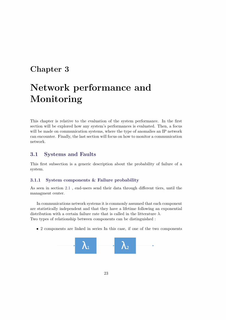
In communications network systems it is commonly assumed that each componentare statistically independent and that they have a lifetime following an exponentialdistribution with a certain failure rate that is called in the litterature λ.Two types of relationship between components can be distinguished :
• 2 components are linked in series In this case, if one of the two components
23

24 Chapter 3. Network performance and Monitoring
fails, subsequently the overall system fails. So, the failure probability of thetwo components in series can be defined as:
F (T ) = Pr[Failure of 2 components in series]= Pr[Failure in C1] ∪ Pr[Failure in C2]= Pr[Failure in C1] + Pr[Failure in C2]
• 2 components are linked in parallel
In this case, in order for the system to fail, it is necessary that both components failat the same time. Then the failure probability of the two components in parallel canbe defined as
F (T ) = Pr[Failure of 2 components in serie]= Pr[Failure in C1] ∩ Pr[Failure in C2]= Pr[Failure in C1] ∗ Pr[Failure in C2]
It is then easily proved that the probability of failure for components in parallelis lower than the ones in series. This subsection was used to prove the necessity ofhaving two different networks, using two different gateways to internet in order toreduce the probability of a failure in the system.
3.1.2 Dependability of the system
A service provided by a system can be defined using a binary relation as shown infollowing figure.
The idea behind this thesis is avoid service’s failures that are more frequentand more severe than acceptable, meaning to have the most dependable service aspossible. In this section, will be presented the necessary attributes to be a dependablesystem and distinct threats a system can encounter.

3.1. Systems and Faults 25
Figure 3.1: Relationship between correct/incorrect service
Attributes
For the attributes of a dependable system, article [17] provides the following defini-tions:
• Availability: It defines the readiness for delivering a correct service by thesystem. In other words, it verifies if at a certain instant t, the system candeliver a correct serve.
• Reliability: It defines the continuity of the services to provide a correct service
• Maintainability: It is the ability for the system to undergo repairs and modifi-cation.
• Integrity: It defines the ability of the system to avoid possible alterations ofthe system.
• Safety: It defines the absence of dramatic consequence for the user and/or theenvironment.
• Confidentiality: This defines the absence of unauthorized disclosure of infor-mation.
It is possible to define the Availability, Reliability and Maintainability in a morequantitative way.
For common smart grid applications (seen in 2.3) applications, the required avail-ability is in the 99–99.99 percent range. However, some critical applications such asSynchrophasors or substation automation, require even better reliability,approximately99.99995 percent, which equates to being out of service for 16 seconds in one year.
Threats
A system can encounter three different threats:
• Fault: It is an event that is the cause of an error. Many different types of faultcan occur, the article [17] distinguished more than 256 different combined faultclasses.
• Error: An error is a deviation for the system from a correct service state, andmay lead the system to a failure.

26 Chapter 3. Network performance and Monitoring
• Failure: A failure is an even when the delivered service is not acceptable orfails to conform a specification of the system.
In the case of multi-component or distributed system, failure in one part can thereforelead to a fault in another part of the system, and consequently, provoke a cascadingfailure off the overall system.
Figure 3.2: Propagation of failures [17]
3.1.3 Concept of Fault Management
Network management tasks must follow by the OSI/ISO network management modelFCAPS (Fault,Configuration,Accounting,Performance,Security), that defines five fieldsfor network management as stated in [18]:
• Fault management: This is the process from the recognition to its resolutionof an abnormal operation of the OSI environment.
• Accounting management: It enables the uses of statistical means in orderto identify the cost of the use of resources
• Configuration management: it identifies, collects and provides data to ini-tialize and start continuous operation of services.
• Performance management : It evaluates the behavior of resources and theeffectiveness of communication activities, to ensure performance remains at thesufficient level. The performance management can gather relevant statisticalinformation for the network.
• Security management : It supports the application of security policies, butalso reports any security events that might threaten the integrity of the system.
In this thesis, a particular care has been taken on the fault management aspectof the FCAPS framework. In real life, it is impossible to have a system that willnever encounter any errors. However, those errors must stay at a reasonable level,in order not to lead to failures. It is then important to design a system capable ofbeing resilient when a fault occurs, in order not to have a or many failures as seen insection 3.1 Instead of the two-state service as seen in figure 3.1, the fault managementconcept is divided into five different steps as follows :
• Detection: A fault is detected on the system, without knowing where on.
• Diagnosis: This is the capacity of determine which component lead to a fault

3.2. Anomalies in the network traffic 27
Figure 3.3: Fault managment steps
• Isolation: It’s the way of make sure that the diagnosed fault will not propagate,leading to a cascading failure.
• Recovery: This is the function restoring the component to its normal state
• Repair: Restoring the system to its expected state.
This thesis will focus only on the detection, diagnosis and isolation steps, andwith a specific care for the two first. The detection and diagnosis procedures will bemore detailed in the following sections. The isolation function has been designed inthe problem formulation. Indeed, when a fault is detected and can lead to a failure,then the smart meters will switch the mean of communication allowing the data tobe send through the backup network.
3.2 Anomalies in the network trafficIn the scope of this project, my goal is to try to prevent any failures in the commu-nication link between an end user and the control center. To do so, the approachwhere the network traffic is monitored to see any anomaly in it has been chosen.
The first step for this way, is to define clearly what is the normal traffic in thenetwork so when an anomaly occurs, there will be a deviation from this regularstate.Those events may be detected while or before a failure of a part of the system,and therefore, are needed to prevent them.
It is assumed the network is using only the IP protocol from the Smart metersto the control center, and consequently, a close attention is payed on two kinds ofanomalies IP systems may encounter.
The first category is all the different types of failures that can happen in an IP-system and the performance problems. This category of an anomaly could be reallybroad and, without being exhaustive. The most familiar ones can be described as :
28 Chapter 3. Network performance and Monitoring
Link corruptions: This refers to a physical damage to the connection, that couldbe a broken cable, a fiber span, etc.
Electrical noise : It refers to instability of the link because of a high electromag-netic radiation, for example, close to high-voltage devices.
Power outage: It refers to a power problem of a device in the network, that couldbe locally situated, or more global. In the case of a power outage for an antenna ora router, this can affect a large number of devices.
Interface damage: This is probably the most common hardware failure, that af-fect for example a router or a switch, leading to a disconnection of a certain area inthe network.
Software issue: When the internal software of a device encountered a bug, andno longer communicates.
Routing Misconfiguration This refers to incorrect routing table, than can lead thetraffic not to be routed in optimal paths, or even in loops.
Packet over-flooding This refers to situations were the bandwidth is occupied byunwanted traffic, for example in the case of broadcast storm
In the litterature, those failures are mainly regrouped in 4 distinct classes
• IP-Connectivity issues
• Physical issues
• Network misconfiguration
• Software issues
The second category of anomalies, is this time human based, and concerns security-related issues. Because the network will be extremely complex due to its open and dis-tributed architecture, an IP network can be attacked from inside or outside. Mainly,this concerns denial of service attacks, but also virtual shutdown of the network orflooding by unwanted traffic due to worms.
All the failures in those two categories have a clear impact on the metrics ofthe network, such as the throughput, the delay, the bandwidth, but also will inducethe fragmentation of packet, retransmission, collisions.Thus, by getting the networkperformance data, it is possible to detect any transient changes in measured networkdata that occur prior or during an abnormal event [19]
The following part will explain what are the different paradigms and strategiesin order to monitor the network, and get the performance data.

3.3. Monitoring and Fault detection 29
3.3 Monitoring and Fault detectionThe monitoring of a network concerns mainly two fields of the FCAPS frameworkdescribed previously in section 3.1.3:
• Fault Monitoring
• Performance Monitoring
The fault monitoring concerns problems in the network. As seen in 3.2, faultscan happen in various layers of the OSI layers, thus, it is important to know whichone is abnormal.The Performance monitoring can measure performance of a network. By observingthe network during non faulty situation, it is possible to establish some efficientperformance "model". Therefore, a faulty situation can be then detected when theperformance of the network tend to be too different from this faultless model.
The way of monitoring a network can be separate into two distinct kind: Passiveand Active monitoring.
Passive monitoring does not generate any additional traffic on the network,and only listen what transit on the specific point(e.g a router), and derive fromit metrics.According to thoses, the probing station may decide if there is a faultysituation or not. Some alarm may be also inherent to the protocol used, such as awrong packetsize, number of retransmission packets. More generally, the article [19]defines somes relevant metrics and what should be the alarm condition inherent andare transcribed in figure 3.1
Among others, common passive monitoring are, for example, Wireshark, Fiddler,or Tcpdump.
Active monitoring involves sending traffic in the network in order to sampleits behavior. One of the principal advantages of active monitoring is that there isa direct choice of which traffic to send, and the probes (i.e the traffic sent) canbe designed in order to measure a specific quantity like average delay, the route,available bandwidth. It is then possible, by observing the network to localize fault,and diagnose it.
Some monitoring standards have been defined and are commonly used, such asthe Simple Network Management Protocol [20], Netflow [21] or the Remote Networkmonitoring [22]. These methods are qualified as Router-Based monitoring techniques.The idea is that the probes stations are localized on certain node of the network, andmonitor the nodes around them. A unique central management center send probingrequest to the stations, that transmit the results afterward. Therefore, as explain in[23], in order to to have a real time monitoring of a highly distributed system, a highprocessing load on probing station along with a high bandwidth consumption mustbe expected. Thus, this may lead to flooding the network due to high frequencymanagement request. Thus, they may behave well in the small-scale network, their

30 Chapter 3. Network performance and Monitoring
Network Metrics Alarm Condition
Out-of-order sequence packets First Appearance
Jumbo or Runts frames First Appearance
CRC error frames First Appearance
TCP Checksum error First Appearance
Collision frames Threshold-based
Fragment packets Threshold-based
Retransmission Packets Threshold-based
Broadcast packets Threshold-based
Packet interarrival time Analysis over monitoring period
Throughput Analysis over monitoring period
Packets per second Analysis over monitoring period
Packet size Analysis over monitoring period
TCP window size Analysis over monitoring period
Table 3.1: Metrics and their Alarm condition in IP networks
performance decrease with the complexity of the network, while flooding the net-work with management requests. Some example of monitoring framework using thiscentralized, or "router-based" approached can be found in [24],[25].
The other approach of active monitoring is to use a decentralized way. There isno more one central management center which collect results from stations, but in-stead, different nodes send for themselves probes and can derive directly the networkdynamics. Therefore, the node does not have an overall vision of the network, butonly of the path the probes took.
One of the inconvenient shared by both approaches is the impact of the probeson the network. The goal is to send enough packets in order to have a relevant mon-itoring, but not too much in order not to flood the network and induce congestion.Two different probing techniques is then possible:
Pre-Planned Probing: This involves a preplanned selection of probes that aresend periodically, and the network state can be determined with probe’s results. This

3.3. Monitoring and Fault detection 31
implies that a large management traffic is generated, that can induce delay, and defacto a certain inaccuracy.Moreover, active probing suffer from a limitation: The probes set are defined inadvance and in an "offline" situation, it is mandatory for it to be able to detect allpotential problems.Two problems arise from that: The first one, is that it cannot be proven that thedesigner of the probes select a complete set of probes all problems imaginable, lead-ing to potential weaknesses. The second is the possibility that probes have beendesigned to detect faults which are unlikely to occur, flood the network for nothing.Furthermore, most of the time, once a fault is detected, the diagnosis may need moreinformation, not available with defined probes[26].
Active Probing: Active Probing is based on an interactive mode, where themost likely diagnosis is determined using the probe’s results. Once a diagnosis hasbeen established, extra probes are selected in accordance, and send to get more in-formation and de facto to refine the diagnosis, this operation is repeated until thedetermination of the problem.
By this way, active probing would be a solution for the preplanned probing lim-itations: The probes are sent to occurring problems, and are dynamically designedfor that problem. Furthermore, the probes can directly focus on the localization ofthe fault, reducing the impact of monitoring the network.
The technical report [26] give a hint about the steps to follow in order to diagnosefaults:
1. A small probe set must be pre-selected, so that when a problem occurs, it ispossible to detect something has gone wrong
2. The probe results must be integrated and analyzed, to determine the mostlikely network state
3. The "‘most-informative"’ probes to send next must be selected based on theanalysis of previous probe results
4. this process must be repeated until the problem diagnosis task is complete
In both active or pre-planned probing, the selection of the probe is then animportant step in order to localize a fault. Various different types can be found inthe literature[27]. Those probes have different ways of interaction in the network, bythe number of packets sent, or the frequency of sending. The principals methods arethe following:
• 1-packet: The pathchar tool describes by V. Jacobson used the 1-packetmethod, to estimate link bandwidth from round trip delays of different packet
32 Chapter 3. Network performance and Monitoring
size, on the assumption than the transmission delay grows linearly with thepacket size
• Packet pair The method use minimum inter-departure time of successivepackets sent back-to-back on a link to estimate the bottleneck bandwidth.Some methods estimate available bandwidth based on the observation of inter-departure time of consecutive probe packets.
• Packet train A Packet train is simply a sequence of multiple packet pairs. Asan example, the Pathload tool uses this method. train.
• Packet tailgating These methods use packet trains, using large packet andsmall packets. Because of their limited TTL, large packet will be discardedmidway, and only the small one will capture timing information. However, ifthe probing bit rate is higher than the bandwidth, this will cause a congestion.Therefore, by knowing the minimum probe rate, it is possible to know theavailablebandwidth.
As examples, the most common probing tools are ping, pathchar,iperf, Cprobe,Skitter, pathrate,PatchChirp,NetTimer.
3.3.1 Choice for the simulation
To sum up, two categories of monitoring are possible : the passive one, which consistin listening the network at certain important point, or the active, that providemetrics by the use of probes send in the network.
In the scope of this thesis, the monitoring must collect data such as end-to-enddelay or the jitter. Therefore, the passive monitoring cannot provide such metricsfor each link between houses and the management center.
For the active monitoring, as described, the probes stations can be placed fol-lowing two different approaches : the router based, or the decentralized one. Twoproblems arise with the first approach: as explained in section 3.1.1, the simulationwill use as primary and secondary network respectively an ADSL connection and aLTE one. This means that data will transit throughout internet, and therefore, themanagement center does not have the capacity of pulling probing command.Moreover, Router-based techniques implies that only the network management cen-ter will get the monitoring information.Yet, in the thesis scenario, both ends need toestimate the network dynamics, which is not the case here. In conclusion, Router-based approach seems then non compatible within the scope of this thesis. Therefore, the decentralized activeprobing seems to be the best way of to obtain end-to-end metrics. However, a par-ticular attention to its scalability and the probes’ impact on the network dynamicsmust be paid.

Chapter 4
Simulation Model
As explained in the previous sections, the general idea of monitoring a smart gridnetwork, is to have a smart meter in each house, sending data periodically, betweenone and fifteen minutes. In a concern to have a more scalable system, the smartmeters send data actually to an aggregator, which then report to the managementcenter. Due to the low frequency of updates, it is important that the messages arewell transmitted between the two end of the network. Therefore, one of this thesis’goals of is to detect if any faults happened inside the network between two messagessend, and if those faults lead to a possible failure of communication, use a secondarynetwork to transmit the data.
Each meter will probes in between the real messages, in order to be sure that thedata can be received properly. If, from the probes results, the primary network isconsidered as faulty, then the message will be send through the secondary network,that has a different aggregator, until full recovery of the first one. This means thatthe main and the secondary aggregator must have a coordination system, to ensurethat if one has a failure, the other handle the connection. If for the same house, thetwo concentrators conclude there is a failure, then the management center must benotified.
As seen in section 2.3, the size of the packets of actual data for smart gridapplication is small: the maximum is around hundred of kilobytes. As seen the report[28], such packet are more sensitive to delay than the bandwidth itself. Therefore,in the simulation, the probes will be used to derive the end-to-end delay of packets,but also the interarrival time of the probes. In the following section, the architectureof the primary and secondary network will be described, and how can the delay becharacterized based on that:
4.1 Networks descriptionAs detailed in section 2.2 the primary and secondary network used are respectivelyADSL and LTE. The ADSL network can be simplified as follow :
From 4.1, it is etasblished that one of the main weakness point of the network
33

34 Chapter 4. Simulation Model
Figure 4.1: ADSL Architecture
is at the DSLAM, which multiplex the data of many users to connect it to the ISPnetwork. Indeed, if many users use intensively the network at the same time, thismight be a typical point for a bottleneck to be formed.
Regarding the LTE network, due to the lack of mobility for the houses, all thecomponents responsible for the handover managment will not be taken in consider-ation. The architechture of the network can be schematised as :
Figure 4.2: LTE network representation
The LTE network is composed by :
• User Equipment : It is modem requirement to connect to the network
• eNodeB : It is the evolution of the UMTS base station, it has the role to connectthe users to the core network of LTE
• Service Gateway : the S-GW allows the users to communicate with other usersof the LTE network but also 2G/3G network. It is also responsible for routingthe packets to the correct eNodeB from the P-GW
• PDN Gateway : This gateway provide the connectivity between the UE andexternal packet data network, such as Internet.

4.2. Simulator description 35
A new feature of the LTE compared to 2G/3G network is the use of ALL-IPconnectivity. This means that all kind of utilisation (voice,voip,data) is treated thesame way. This feature reduce the number of steps necessary to connect the user tointernet. This lead to a important improvement of the latency, with usual latencybelow 30ms for data smaller than 1Kilobyte.LTE use as coding the Orthogonal Frequency Division Multiple Access. This mod-ulation is at the same time a frequency and temporel multiplexing. The use oforthogonal frequency reduces the interference caused
In conclusion, the final system architecture that will be used during the simulationcan be seen in figure 4.3
Figure 4.3: Simulation system architechture
From this definition of the network model used in the thesis, the following sectionwill focus on the implementation in the network simulator OMNeT++.
4.2 Simulator description
4.2.1 OMNeT++
OMNeT++ is an open source discrete event simulation package written in C++.OMNeT++ has been designed to enable large scale simulation, with hierarchichal,and customizable modules.
OMNeT++ use a modular language named NEtwork Descrption (NED), whichallows the modelisation of complex systems by assembling several elementary mod-ules together. The architechture of the network is described following a hierarchichalorganistation, with the following components:
• Simple Module: It is a single component that allows us to define the algorithmiccoportement
• channel: It is the link that ensure the liason between modules

36 Chapter 4. Simulation Model
• Compound module: a structure composed by simple modules connected t
Active modules, also named simple modules are derived from a framework base class,cSimpleModule. Those active modules, can be regrouped in a hierarchichal way inorder to form compound modules. Unlimited different hierarchichal layers of com-pound modules can be created in order to make a system module. Modules commu-nicate between each others using messages; those are send either by direct connectionbetween modules(input/output gates) or directly to the destination modules.
Figure 4.4: Model Structure in OMNeT++ [29]
Once modules different modules are built, the network model can be defined usingthe NEtwork Description (NED) language particular to OMNeT++. NED languageis used to described which module are used, to define the topology of the network, theinterconnections between the modules, and the parameters of the compounds. TheTopology of the network can also be defined using the user interface of OMNeT++,which translate automatically into code the different modules. The figure 4.5 showas example the way two host are connected together, using the graphical interface,or the ned language.
Figure 4.5: Graphical (left) and Ned-based (right) Network description
Once the simulation model described in NED or the module behavior written inC++ are completed, the simulation parameters are stored using INI files. While the"backbone" of the simulation (NED and C++ files) is assumed to stay unchanged,some parameters vary according to the experiment. Therefore, all parameters aresaved seperately in an INI file. Using this differientation allows us to have multi-ple scenarios, to observe how the simulation behave according to different inputswithouth having to change the models files.

4.2. Simulator description 37
OMNeT++ is a simulation environment, where the standard modules are genericto fit in any basic scenario. However, due to its modularity each module can beeasily reused in any other module, which has lead to the developpement of diverseframework on top of the simulation environment.
4.2.2 INET
The INET framework for OMNeT++ is the keystone of the simulator : while OM-NeT++ only implement generic modules, the INET framework add up a full libraryof standards use in an internet networking. On top of protocols issued from the OSIlayers, INET also implements several applications models, mobility support, routingprotocols and is responsible for the configuration of the IP network (IPv4/6). There-fore, this framework is essential in order to have realistic simulation. The figure 4.6show for example the difference between a regular OMNeT++ host and one usingthe INET Framework.
Figure 4.6: Comparision between OMNeT++ Host(left) and INET-extended Host(right)
4.2.3 SIMULTE
The SimuLTE is a framework developped to evaluate the performance of LTE andLTE-Advanced networks. The framework implements the core network of 4G net-works as described in section 4.1, but also the eNodeB, and the physical and Maclayer for the Users Terminals. Regarding the rest of the OSI layer for the Users ter-minals, SimuLTE is based on the INET framework, insure a full compatibility withother INET modules.

38 Chapter 4. Simulation Model
4.3 Network description in OMNeT++From the OMNeT++ point of view, the network described in 4.1 can be seen fromthe simulator interface as:
Figure 4.7: Omnet++ Representation of the network
This section will cover the different OMNeT++/INET/SIMULTE modules usedin order to reproduce this network.
4.3.1 IP Adress attribution
To function properly, each nodes of the network must have an defined IP adress. Todo so, OMNeT++ implement two modules: IPv4NetworkConfigurator and IPv6NetworkConfigurator.The role of this configurator is to assign each interface a unique adress, and to definestatic routes. The attribution can be either done automatically by the module, or canbe configure manually. In this case, the configuration file must be store in an XMLfile. This XML file must contain one <config> element, and then may contain multi-ple parameters elements from :<interface>,<wireless>,<route>,<multicast-route>.
The <interface> provides configuration attribues for one or many interface of thenetwork. These are :
• hosts: Selector that specifies the hosts that must be affected by the interfaceelement
• name: Selector attribute that specifies the name or a list of interface name. Bydefault, it is set to "*" (All names)
• towards: Selector specifing a list of host names connected towards the specifiedhost
• among: Selector specifing a list of host names to whom the specified host isconnected
• address: Parameter limiting the range of assignable addresses. Possible to leaveunspecified part such that the configurator fill it automatically eg:"10.0.x.x"

4.3. Network description in OMNeT++ 39
• mtu: Parameter to set the MTU in the interface
• netmask: Parameter limiting the range of assignable netmask. Possible to leaveunspecified part such that the configurator fill it automatically eg:"255.255.x.0"
• groups : Parameter to assigned a list of IP address to add in the multicastgroup of the interface
The <multicast-group> is used to provide multicast network addresses for theinterface of the network.
The <wireless> is used to described any wireless network, with the followingattributes:
• id: Parameter to identify the wireless network
• hosts: Selector that specifie a list of host names
• interface: Selector that specifie a list of interface name that will be affected
The <route> allows to provide manual routing table for multiple node. Thescope of those route are delemited by the following attributes :
• hosts: Selector that specifies the hosts that must be affected by the interfaceelement
• destination: Selector attribute that specifies the destination adress in the route.
• netmask: Parameter that specifies the netmask in the route.
• gateway: Paratemer specifiying the next hop adress in the route
The <multicast-route> defines the multicast routing tables, by specifying from whichinterface multicast packets are expected (parents), and to whom those packets aresend (children).
As example, considering the following test-network:The configutation file may contains the following (but not exhaustive) xml code:
<config><interface hosts="host1" towards="router1" address="172.0.0.1" netmask="255.255.255.0" mtu="1500"/><interface hosts="host4" towards="router3" address="172.0.1.1" netmask="255.255.255.0" mtu="1500"/><interface hosts="router2" towards="router1" address="172.1.0.1" netmask="255.255.255.0" mtu="512000"/><multicast-group hosts="host1 host2 host3" towards="router1" address="225.0.0.1"/><route hosts="host1" destination="*" netmask="/0" gateway="router1" metric="0"/><route hosts="router1" destination="host1" netmask="/32" metric="0" interface="ppp0"/><multicast-route hosts="router1" groups="225.0.0.1" children=">host1 >host2 >host3"/><\config>
At the network initialisation, the configurator will first take the configuration fileand apply it. If some interface or routes, are not defined, it will assign it automati-cally. Once the network is configured, each node in the network must have inside thenetwork layer a module named IPv4NodeConfigurator (or IPv6NodeConfigurator)that actually set the node’s interface table and routing table based on the informa-tion defined by the IPvxNetworkConfigurator.

40 Chapter 4. Simulation Model
Figure 4.8: Test network for IPv4NetworkConfigurator
4.3.2 LTE BINDER
The LTE BINDER is a similar module as the IPvxConfigurator seen previouslyused with SimuLTE. It has only one instance in the whole network, and is called atthe initialisation of the network. The Binder stores the mapping tables with otherOMNeT++ module (not part of SimuLTE). First, the binder assigned the IP andmac Addresses for lte modem, then bind the User equiments to an eNodeB and definewhat is the next hop for each eNodeB in case of Handover. During the simulation,the Binder is used by the eNodeB to acces the nexthop table, by any module toaccess the others OMNeT module’s ID, and to get the map of already deployed UserEquipments in order to have some Adaptive Modulation & Coding (AMC).
4.3.3 Channel Controler
The Channel Controler is a mandatory module in OMNeT++ if the simulated net-works use wireless communications. The controller is responsible to locate everymoving node in the network, and determine which nodes can interfere with others.Then, the radio interface of the node reuse this paramet during the transmission.The Channel Controler is also responsible to enable and set up the radio tranmissionchannel parameters. In the case of a LTE network, the channel parameters are :
• Shadowing
• Pathloss scenario
• Height of eNodeB
• Carrier Frequency
• Target Block error rate
• Harq reduction
• Antenna Gain: UE and eNodeB

4.3. Network description in OMNeT++ 41
• Thermal Noise
• Noise figure : UE and eNodeB
• Fading type
• InCell and Inter-cell interference
SimuLTE provide different XML scripts implement those parameters with differ-ent values, or model type.
4.3.4 Hosts
The aggregators and the managment center are defined as Standard Host, while thehouses are defined as a Standard Host with an LTE interface added. The internalstructure of an host has been shown in figure 4.6.
The host is composed in 4 layers disposed in a hierarchichal way, which correpondto the OSI layer.
• The first layer is for the interfaces such as ethernet, point to point or LTE.
• The second is the network layer, using either IPv4 or IPv6
• The third correspond to the transport layer, and implements TCP, UDP andSCTP
• The last correspond to the Applications using protocols of the transport layer.
The 3 first item cited are used in a "transparent" way for the user, meaning thatno configuration is necessary prior the simulation. However, the application layer isdefined in a generic way, assuring only the interconnection to the transport layer.Each application must inherit from this generic application. This way, many applica-tion can run at the same time. Inet provide as examples different types of applications

42 Chapter 4. Simulation Model
INET UDP Applications :
• Basic Client: An application sendingperiodically packets
• Burst: Same as the Basic client, butpackets are send in a bursty way
• Echo: Send back any incomingpacket
• Video Streaming client: Send videostream request
• Video Streaming server: Send avideo after receiving a request
INET TCP Applications :
• Basic client : A simple request-response application over TCP
• Echo: The server Echo incomingmessage
• Telnet: A telnet session
• Sink: Any incoming packet aredropped
• Session: Opens a connection, sendsa number of byte and closes
• Server: Server to handle TCP-basedapplication
Those examples are a nice introductory way to design further advanced applica-tion.
4.3.5 Internet Core Network
To emulate the internet core network, the INET framework has a specific modulenamed "Internet Cloud". This module allows to have a more accurate representationof the core network. This component takes many different parameters as input• src : It is the source of the packet
• dest : Destination of the packet
• delay: the time the packet will wait before reaching the destination
• datarate: the throupghut of the link
• drop: the probability that the packet is dropped.The internetCloud module allows to have different routes with different delays
and drop probality. In order to have a clear input, those routes can be stored in aXml file. An example of xml file is given below<traffic src="router1" dest="router2" delay="10ms+truncnormal(5ms,5ms)"datarate="uniform(10Gbps,100Gbps)" drop="uniform(0,1) < 0.01" />
From this example, it can determined that the Cloud network is located betweentwo router, the delay between the two router is following a normal distribution with amean of 15ms with a deviation of 5ms. The datarate is uniform between 10Gbps and100Gbps, and the probability that a packet is dropped is les than 0.01. Regardingthe drop probablity, the term "<" correspond to the sign "≤" (less or equal) in xmllanguage.

4.3. Network description in OMNeT++ 43
4.3.6 Scenario Management
According to the experiment, users may want a change of parameters,eg. a routesupression, an increase of the bit error rate of a connection, in order to examine thetransient behaviour of the network. To do so, the user may want to do it manuallythrough the graphical interface. However this is a long process, and in the case ofmany experiments to run in a row, it can get a fatisdious task. Therefore, OMNeT++implement a module named ScenarioManager in order to automatize the schedulingof certain events. The ScenarioManager executes a set of built-in commands thataccept parameters. Those commands are:• <set-param>: Select and modify a parameter’s value for a specific module.
• <set-channel-attr>: Modify an attribute of the channel connected to the gateof a module
• <connect>: Connect two gates of two modules with a channel defined with<param>
• <param>: Used inside the <connect>, to fix the channel attributes.
• <disconnect>: Disconnect the gate of a moduleFor each command in the script, a time "t" must be specified so that the Manager
can schedule the events. For a same time, either one or many event can be schedule.The following example show a script with 7 events at 4 different times.
<scenario><set-param t="10" module="host[1].mobility" par="speed" value="5"/><set-param t="20" module="host[1].mobility" par="speed" value="30"/>
<at t="50"><set-param module="host[2].mobility" par="speed" value="10"/><set-param module="host[3].mobility" par="speed" value="10"/><connect src-module="host[2]" src-gate="ppp[0]"
dest-module="host[1]" dest-gate="ppp[0]"channel-type="ned.DatarateChannel">
<param name="datarate" value="10Mbps" /><param name="delay" value="0.1us" />
</connect></at><at t="60">
<disconnect src-module="host[2]" src-gate="ppp[0]" /><disconnect src-module="host[1]" src-gate="ppp[0]" />
</at></scenario>
The ScenarioManager allow to schedule event in order to modify parameters.However, it is incomplete regarding any failure a node can experience. To correctthat, a module named LifeCycleController has been developped in starting INET-2.2.0. The LifeCycleController introduce three type of commandes scriptable by thescenario manager : NodeShutdownOperation, NodeCrashOperation and NodeStart-Operation.
The way those operations are scripted are slightly different from other scenarioevents: The script first indicate that this is a lifecycleController operation, thenwhich operation is used and finally in which node the event occurs.

44 Chapter 4. Simulation Model
<at t=’3s’><tell module=’lifecycleController’ operation=’NodeShutdownOperation’ target=’Router1’/></at><at t=’6s’><tell module=’lifecycleController’ operation=’NodeStartOperation’ target=’Router1’/></at><at t=’10s’><tell module=’lifecycleController’ operation=’NodeCrashdownOperation’ target=’Router1’/></at><at t=’11’><tell module=’lifecycleController’ operation=’NodeStartOperation’ target=’Router1’/></at>
4.4 Internet Traffic Description
4.4.1 Periodicity of the Traffic
It has been proven that the internet traffic follows a weekly and daily periodicity.The Danish Internet Echange Point (DIX)[30] provides the following graph for thedaily and weekly traffic graph at the beggining of may 2014:
Because the internet traffic, but also the electricity consumption, is similar foreach day of the week, the simulation will only cover 24 hours cycle. Unfortunately,simulate a 24H hours cycle would need too much ressources, and even more capacityof storage for the results that are not possible.It has been seen from the network description in section 4.1 that a possible bottleneckis at the gateway between the access network and the core network. If a congestionmay occur, it is therefore most likely that it happens at the end of the day. There-fore, the simulations will focus on that specific timeframe of the day, simulating theequivalent of four hours during the spike of consumption.
4.4.2 Delay characterisation
As stated previously, the principal metric this thesis focus about is the delay.Usingthe network architecture, it is possible to have an estimate of what will be the delayin a regular case.
As seen in the figure 4.9, the delay can be decomposed in 3 types:
• Θ(τn) : The delay for a message within a link
• Θ(CN) : The delay of packet within the internet Core Network
• Θ(qn) : The delay a message spend in a queue
• Θ(pn) : The processing time at the meter/server level.

4.4. Internet Traffic Description 45
Figure 4.9: Decomposition of the delay
The values of Θ(τn) are assumed to be following a normal distribution, with asmall variance. The processing time at the house and the aggregtors are assumed totend to zero. The article [31] estimates that the access network as a delay around20ms, the delay in the internet core network is between 10ms to 20ms. It is assumedthat the time at the corporate network is small, less than 5ms. The time each packetspend in a queue depend on the load of the queue. When it is empty, the time iszero, and, a contrario, tend to infinity when it’s congestionned.
From those metrics it can be assumed that the delay of packets using the primarynetwork from one house to the main aggregator will follow a uniform distribution.The following graphs show different example distributions the measured delay fromthe probes will likely follow, in the case of en empty queue.
0 0.01 0.02 0.03 0.04 0.05 0.06 0.07 0.08 0.09 0.10
0.2
0.4
0.6
0.8
1
time in seconds
Den
sity
pro
babi
lity
µ=40ms,σ=3msµ=45ms,σ=5msµ=50ms,σ=5ms
Figure 4.10: Cumulative density function of theoretical end-to-end delays
The same reasoning can be applied for the secondary network : the technicalreport [28] stated that theoretical delay between an user equipment and the PDNgateway is between 20 to 30ms.
4.4.3 Queue description
From the previous subsection, it can be seen that the time each packet send in the thequeue of the DSLAM or routers is the main unknown variable for delay calculation.In the simulation, two type of queue will be used, and are described in the followingparagraphs.

46 Chapter 4. Simulation Model
Tail Drop:
The tail drop is the most simplistic queue model running the following algorithm:
Algorithm 1 Tail Drop Algorithm1: for all New Packet incoming do2: if Queue size ≥ Queue Capacity then3: Drop Packet4: else5: Store Packet6: end if7: end for8: test
The idea is that the queue is serving the packets according to a First In FirstOut ( FIFO) scheduling and has a limited storage capacity. Any new packets areaccepted in the queue until being full, where any new incoming packet are dropped.
In case of congestion, all host using the TCP protocol, whom packet are in tran-siting through this queue will enter in a slow-start, reducing therefore the throughputof all host (TCP global Synchronisation) . This queing management does not differ-entiate any packet, and therefore are all traited the same way.
With this type of queue, a congestion can be detected only when the queue is fulland the packet are dropped, and therefore it is too late to prevent congestion. Thisprocess is done when the average queue is higher than a fixed threshold.
Random Early Detection
The Random Early Detection (RED) is a queuing management widely usef, designedto avoid congestion at the gateways level. The goals of RED is to control the averagequeue size in order to prevent congestion, TCP global synchronisation (as seen forthe Tail Drop), and biais again any bursty traffic.
The principle of RED is that the gateway can detect congestion using the com-putation of the average queue size. This average is kept as low as possible in orderto be able to have fluctuation in the actual queue size, and accomodate with burstytraffic. The idea is to pro-actively try to reduce the throughput of some connection,using congestion mechanisms that transport layers may have, to avoid the conges-tion. Therefore, RED algorithm works well in presence of TCP flows.
The general algorithm for the RED can be defined as :The average size of the queue is calculated using an exponential weighted mov-
ing average and the result is compared with two fixed thresold: the minimum and

4.5. Faults detection Algorithms 47
Algorithm 2 General RED algorithm1: for all New incoming packet do2: Calculate average queue size avg3: if minthresold ≤ avg ≤ maxthresold then4: Calculate marking probability pα5: According to pα, drop incoming packet6: else if maxthresold ≤ avg then7: Mark packet8: end if9: end for
maximum. If the average is below the minimum, no packet are marked. A contrario,if it is above the maximum, all packet are marked.When it is in between the two boundaries, each packet is marked with a probabilitypα, where pα depend on the average. The probability pα correspond to the probablityof being droped. By dropping packet before the queue if full, the RED algorithm tryto trigger congestion mechanism of transport layer, in order to avoid the overflow ofthe queue.
The detailed algorithm of the Random Early Detection can be found in the article[32] One of the option of the RED gateway is to measure the queue in byte insteadof packets, which influence the Using this principle, the pα calculation. This way, alarge packet has more chance to be marked than a smaller one.
The Random early Detection method is more "fair" regarding the use of theavalaible bandwidth and allowing a better treatment for bursty traffic using onlyfew ressources. This protocol effiency rely on transport layer’s congestion avoidancemechanisms. However, protocol such as UDP does not have those mechanism, whichlead to a reduction of the performance of this queuing management [33] [34].
For the simulation, both of this queue management will be implemented, to seethe influence of the queuing time on the delay.
4.5 Faults detection AlgorithmsIn section 3.3, it has been explained that the fault detection system will use activeprobing techniques. This implies that the host send probes to a target in the network,derive metrics from those probes, and can evaluate the situation of the network. Thefault detection process are separated in two : First the collection of network dataand the fault detection process itself.
In this experiment, two type of metrics are collected : The one-way delay andthe interarrival time of the probes.
As seen in section 4.4.2 the delay follows a normal distribution with a certainmean. Using a moving average process to calculate the mean delay for a link, it is

48 Chapter 4. Simulation Model
possible to observe any variation in the distribution. Furthermore, due to the smallvariance of this distribution, even two distribution with a smal difference in theirmean can be easily distinguised.Furthermore, because the smart grid application must fulfill certain delay require-ment, as seen in section 2.3, it is easily possible to dinstinguish faulty and faultlesssituation.Therefore, a thresold decision based algorithm can been chosen as faultdetection system.The following figure shows an example of this threshold process. In this case, thedelay for a faultless case has a mean of 42ms. Then, a failure leading to an in-crease in delay on a link has happened, and a shift of the distribution is noticeable.When the distribution cross the 70ms mean threshold, then the system consider thisdistribution as the result of a failure.
0 0.01 0.02 0.03 0.04 0.05 0.06 0.07 0.08 0.09 0.10
0.1
0.2
0.3
0.4
0.5
0.6
0.7
0.8
0.9
1
time in seconds
Den
sity
pro
babi
lity
End−to−End Cumulative Density Function
µ=40msµ=50msµ=60msµ=70msThreshold
Figure 4.11: Distribution shift after a failure and Threshold
Because the incoming and outcoming traffic is not the same at both end of thenetwork, two similar faults detection algorithm has been designed, one from theHouses’ point of view, the other from the aggregators point of view. The process foreach end will be descrined in the following section:
4.5.1 Fault detection - House’s Point of view
Data Acquisition
The data collection and metrics derivation from the house point of view follows thestep presented in figure 4.15.

4.5. Faults detection Algorithms 49
The calculation of the delay and the Interarrival are based according to the fol-lowing formula:
Delay = Current T ime − (Timestamp of the packet)
InterArrival = (Time of arrivalCurrent packet)−(Time of arrivalPrevious Packet)
In a communication network, some packet may exceptionnaly have a high delaywhile the connection itself is faultless. In order to prevent false positive errors,the fault detection process will use average values for the delay and the interarrivaltime rather than instantaneous value. Therefore, the sample size determinationhas a crucial importance on the outcome of the average calculation process. Theimportance of this parameter will be explored during the simulation phase.
Timeout Process
Despite the good efficiency of these algorithms to detect faults using the probes data,one problem arise when a failure leads to an absence of probes. If the average delaysand interarrival time are collected for a server are collected just after receiving a probefrom the server, then when no probes are received, the averages remain unchangedand the fault cannot be detected.
This is why a Timing process has to be implemented.After each probes, the current time is saved along the other metrics. By this way,
the system can know when the last probe from the server is received. The processwill inspect for the server the last time a probe was received. If the time differenceis higher than the threshold fixed for the interarrival time, then a timeout routine islaunch, and a new average is calculated. Doing this way, it prevent the possibilityof false positive in case of one timeout, and emulate the data acquisition with a newinterarrival time input that increase the average. Therefore, the value of the data addinto the average, and the sample sized used have an influence the delay between thefault and its detection. The following figure shows the number of Timeout routineneeded to detect a fault, according to the new value added to the moving averagecalculation, and by the fault threshold that has been fixed in order to detect a fault.
One of the direct consequence of the previous figure, is the actual time neededto detect the fault, that this time will depends on the frequency of the timeoutroutine, but also the frequency of the probes. If probes are sent periodically everyfive seconds, then even with a threshold equivalent to four times the mean valueafter the initialisation (which is the basis for the threshold decision) is equal to atime close to twenty seconds. A contratio, with probes sent every fifteen seconds,such a threshold is not possible, because equal to the period of actual smart griddata (every minutes). The time required to detect a fault can be derived as
Time = Threshold + (number of steps) ∗ frequencyupdate

50 Chapter 4. Simulation Model
Figure 4.12: Timeline of a Timeout scenario, House point of view.
Restauration Process
When a fault is detected among the primary network, the house decide to switch thenetwork and start sending the data to the secondary network. However, the use ofthe backup network must be limited in time and therefore, the house must be able todetect when the main network is back to a faultless situation. The figure 4.14 showan example timeline of events that will lead to restaure the communication with thehouse and the main server.
Therefore, the fault detection process must also detect when the network becomefaultless again. This will be described in the next subsection.
Fault detection process
Unlike the data collection that is called everytime a new probes packet is incoming onthe socket, the fault detection process run in an independant way and periodically.From this periodicity, it can be concluded that the time period used is a critical aspectin the process. This process works as described by the figure 4.15. As explainedearlier, a thresold decision has been chosen in this case. After the data from theprobes is acquired, the average delay and interarrival time for the last N packets

4.5. Faults detection Algorithms 51
1 1.5 2 2.5 3 3.5 4 4.5 50
1
2
3
4
5
6
7
8
9
10
11
Threshold according to initial mean value
Cou
nt o
f Tim
eout
cal
lsNumber of Timeout calls before detection, sample size=10
NewValue=ThresholdNewValue=1.5(Threshold)NewValue=2(Threshold)NewValue=3(Threshold)
Figure 4.13: Number of Timeout routine needed to detect a fault
(N being the sample size) is calculated. Then, these averages are compared to thethresold, and a decision is made. However, according to the destination server (MainServer or Backup), the number of steps for the process differs. If the destinationserver is the main server, the house will not verify if the Backup server is functionnal.Indeed, it is assumed that as long as there is no connection between the house and thebackup server, this server does not send any probes. This decision has been madeconsidering that the backup server use a telecomunication network that does notbelong to the energy providers and that the amount of traffic need to be minimisedin order to reduce the fees.
This conclude the description of the fault detection from the Houses’ point ofview, and the following part will be dedicated to describe the algorithms used in thesimulation from the aggregator’s one.
4.5.2 Fault detection - Aggregator’s Point of view
While the House must consider only two concentrators (primary and backup), theaggregators must handle the connection of all the houses at the same time. Thishas an influence on the processing time of the packet, but also can provide a moreaccurate view of the network. Furthermore, it allows the management center tolocate the point of weakness in the network when a failure happens. The timeoutprocess being the same as for the one used in the House’s, it wont be discussed.

52 Chapter 4. Simulation Model
Figure 4.14: Timeline of the restauration process from House point of view
Data Acquisition
The data collection and metrics derivation from the aggregator point of view is rathersimilar to the House’s one, but one step is added as show in figure the step presentedin figure 4.16 :
The collection of data is then the same except the last step which consist onhaving an average of the mean delay and interarrival time for each link. This overallaverage is used to have an idea of where the fault is located, and will be discussedafterwards.
Coordination Process
When an aggregator detect a fault for a link, it does not know what kind of faultit is, and if at the other side, the house send data to the backup aggregator. Twoscenarii arise :
• The house has detected the fault, and send message to the backup network
• The house has not detected the fault, and still tries to send the data throughthe primary network

4.5. Faults detection Algorithms 53
Fig
ure
4.15
:Datacolle
ction(up)
andFa
ultde
tection(lo
w)algorit
hm
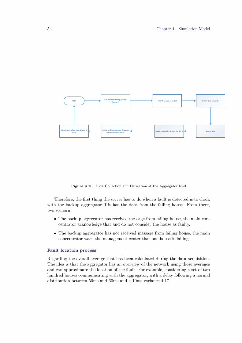
54 Chapter 4. Simulation Model
IDLEFor each incoming probes
(packet)Derive One-way delay
Derive JitterSave instant delay & Jitter for this IP
Find IP-source of packet
Update and save average delay and average Jitter for the IP
Update overall average delay and jitter
Figure 4.16: Data Collection and Derivation at the Aggregator level
Therefore, the first thing the server has to do when a fault is detected is to checkwith the backup aggregator if it has the data from the failing house. From there,two scenarii:
• The backup aggregator has received message from failing house, the main con-centrator acknowledge that and do not consider the house as faulty.
• The backup aggregator has not received message from failing house, the mainconcentrator warn the management center that one house is failing.
Fault location process
Regarding the overall average that has been calculated during the data acquisition.The idea is that the aggregator has an overview of the network using those averagesand can approximate the location of the fault. For example, considering a set of twohundred houses communicating with the aggregator, with a delay following a normaldistribution between 50ms and 60ms and a 10ms variance 4.17

4.6. OMNeT++ Implementation 55
0 0.01 0.02 0.03 0.04 0.05 0.06 0.07 0.08 0.09 0.10
0.1
0.2
0.3
0.4
0.5
0.6
0.7
0.8
0.9
1
Delay distribution for each HouseAverage distribution for the houses
Figure 4.17: Distributions of houses and mean distribution, Faultless situation
This set of house are in a faultless situation , and the aggregator has an overviewof the all set. If one or a few house are failing and the others are normal thisshould have a little influence on the global average.If the aggregator detects a failurefor a house, but the overall average looks normal, then the failure is considered asinherent to the house only. On the opposite, in case of a major failure is happening,but only a few houses are considered as failing during the fault detection process,the overall average will be irregular and the aggregator can conclude that this is aglobal phenomenon and inform the control center.
By using this process, if the aggregator detect that a large failure is happening,the management center can remotely inform the houses to switch the network, eventhough the houses themselves hae not detected any fault.
4.6 OMNeT++ ImplementationIn this section, the main part and key component to design the fault detectionsystem will be discussed. To implement this process in OMNeT++, it was necessaryto design an module at the applicative level. Considering that the probes are sentover the UDP protocol, but the actual smart grid data are sent over TCP protocol,an application implementing both protocol was needed. However, a multi transportprotocol application does not exist in OMNeT++, and therefore it was necessary todesign it entirely.
The mandatory step to implement a new type of application, was to produce ageneric interface, through a module implementing one input/output gate with the

56 Chapter 4. Simulation Model
UDP implementation, one input/output gate with the TCP implementation.
Figure 4.18: UDP-TCP generic interface
Then, during the definition of the application using the NED language, the in-heritance from this generic interface must be stated, along with all the parametersrequired to have an UDP application, and a TCP application.
Figure 4.19: NED implementation of the meters application
One the ned file is described, then the way the application behave must be writtenin C++. After the initialisation of the application, the paramaters are handed fromthe configuration ini file and saved in memory.
The next step to build an application is to create and parameter UDP and TCPsockets from the application. The following figure show the configuration configu-ration for the UDP socket, the initialisation of the TCP sockets follows a similarprocess.
Once those two steps are completed, then the application itself can be designed.

4.7. Data collection- Signal mechanism 57
4.7 Data collection- Signal mechanismOMNeT++ has two way to do gather data from the simulation modules:
• The Collectors
• The Signals
The collectors are a classic approach of gathering data. The collector need to behardcoded in the C++ code, and a collector can only describe one type of statis-tics(vector, scalar or histogram).
The Signal is a softer way to collect statistics. This mechanism allows us tocollect a temporal serie of information S =xt where xt is the information at time tof the signal S.
This information is collected using fuction named emit(S,value),where value cor-respond to xt. One of the advantages of the signal is the that any modules cansuscribe to a signal, and be notified when the signal is emited. For example, whenthe aggregator’s fault detection module emit a fault signal, the module responsiblefor the coordination with the backup network is notified and start sending messageto the second aggregator.
@signal[delayPk](type="double");
Moreover, diverses types of statistics(mean,variance, histogram) can be collected todo post-mortem analysis of the simulation.
@statistic[endToEndDelay](title="end-to-end delay"; source=delayPk; unit=ms; ...record=histogram,vector; interpolationmode=none);
The signals are stored after the simulation in two files, one that contains thescalar results, and the other the vectors results. Those files can be handled directlyusing the statistical software R, or by exporting by hand the vector desired into aCSV file.

58 Chapter 4. Simulation Model

Chapter 5
Results
In this chapter, the experiments conducted will be presented, and discussed.
5.1 Parameters and variablesIn this first section, the different scenarii’s parameters and variables used for theexperiments will be detailed.
5.1.1 Random Number Generation
The generation of random numbers is a important step in any simulation : the qualityof the random variables influence directly the quality of the results. In OMNeT++,the pseudo random generator by default is the Mersenne Twister. This PRNG isused in many tools and language and has the following propriety:
• The periodicity is 219937 − 1
• It can produce 623 indepent sequence of 32bits numbers, uniformly repartited
It is also possible to use others PRNG such as the L’Ecuyer generator or theLinear Congruantial Generator.
The seed is responsible for the suite of generated number. It is then primordialparameter to select. In OMNet++, the seed of each simulation can be specified inthe ini file. Therefore, in this thesis, for each simulation a different seed is selected.This make possible to have a different simulation every time instead of a repetitionof a previous simulation. Moreover, in order to discard the data produced duringthe transient phase of the PRNG, OMNe++ include a parameter named Warmupperiod, which correspond to the time no results will be stored. Finally, in order tohave more statistically accurate results, each experiment is repeated 10 times, andthe results stated are average of all the replications.
59

60 Chapter 5. Results
5.1.2 Simulation parameters
The parameters used in the experiment defined the different scenarii and help tomake the distinction between experiments.
The first parameter is the number of houses. The primary network is an emulationof an ADSL network, and DSLAM is composed by several aggregation cards. Thoseusually contains 24,48 or 72 ports. The simulations will therefore use 72 houses.
The Smart Grid application emulated in the experiment is a metering application.This means that the size of the data send are in the order of X and the frequency ofdata send is between 1 and 15 minutes. In the simulation, the actual data are sendevery minutes.
5.1.3 Simulation variables
In the previous chapter, five parameters used in the fault detection algorithm andhaving a direct influence on the simulations’ results have been defined:
• Frequency of the probes
• Frequency of the fault detection routine
• Samples size for the average calculations
• Threshold definition
• Timeout process
Therefore, the first experiments realized are how does the variation of thoseparameters affect the fault detection process.
In order to first verify that the fault detection process is fuctionning correctly,experiments are made with a network under a light load (no dropped packet at thegateways), but with scenarized faults. This way, the performance of the algorithmcan be evaluated. The scenarized faults are
• Gateway shutdown for one minute
• Increase of latency for one link (House to Gateway)
• Increase of latency for several links
• Increase of latency for all links
5.2 Fault Detection
5.2.1 Caracterisation of the Delay and Inter-arrival rate
The fault detection algorithm used in the thesis stands on the assumption that thedistribution of the probes would be normally distributed, and the decomposition

5.2. Fault Detection 61
of the delay in section 4.4.2 was indicated the delay would be between 40ms and45ms. The first step of the experiment was therefore to analyse the delay in thesimulation, to verify this assumption. To do so, the data of 3 hours simulations havebeen collected , where the network is in a light load.
The empirical cumulative distribution is shown in figure 5.1, along with theoret-ical distributions.
0 0.01 0.02 0.03 0.04 0.05 0.06 0.07 0.08 0.09 0.10
0.2
0.4
0.6
0.8
1
Time in seconds
Pro
babi
lity
Den
sity
Comparison of theoretical and OMNET−based end−to−end delay distributions and
µ=40ms,σ=5msµ=45ms,σ=5msOMNET Simulated
Figure 5.1: Comparision of theoretical and Results for end-to-end delay
It can be seen from the distribution that the end-to-end delay seems to followsimilar to what was described in section 4.4.2. This result was predictable, and isused here as a confirmation. The delay among links is a parameter in OMNeT++,so it was expected to be around 42ms. This shows also that the assumption thatthe delay will be following a normal distribution, used in the detection algorithm, iscorrect.
5.2.2 Router Shutdown
The first step in the experiment was to verify that the algorithm was functionning.To do so, the first experiment conducted was in the case of a router failure, at thegateway level. This failure was simulated using the lifeCycleManager component inOMNeT++, and the operation used was a "NodeShutDownOperation". This meansthat the router interface was at some point turned off, and all incoming packets weredropped. The failure of the router implies that the interarrival time will increase,and the timeout routine will be called until the failure detection.
The following sets of plots will shows the performance of the algorithm withdifferent values for the variables detailed previously in subsection 5.1.3.
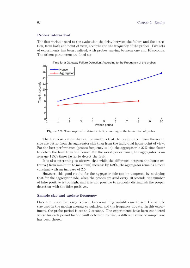
62 Chapter 5. Results
Probes interarrival
The first variable used to the evaluation the delay between the failure and the detec-tion, from both end point of view, according to the frequency of the probes. Five setsof experiments has been realized, with probes varying between one and 10 seconds.The others parameters are fixed as:
0 1 2 3 4 5 6 7 8 9 100
2
4
6
8
10
12
14
16
18
Probes period
Tim
e in
sec
onds
Time for a Gateway Failure Detection, According to the Frequency of the probes
HouseAggregator
Figure 5.2: Time required to detect a fault, according to the interarrival of probes
The first observation that can be made, is that the performance from the serverside are better from the aggregator side than from the individual house point of view.For the best performance (probes frequency = 1s), the aggregator is 22% time fasterto detect the fault than the house. For the worst performance, the aggregator is onaverage 115% times faster to detect the fault.
It is also interesting to observe that while the difference between the house ex-trema ( from minimum to maximun) increase by 159%, the aggregator remains almostconstant with an increase of 2.5
However, this good results for the aggegator side can be tempered by noticyingthat for the aggregator side, when the probes are send every 10 seconds, the numberof false positive is too high, and it is not possible to properly distinguish the properdetection with the false positives.
Sample size and update frequency
Once the probe frequency is fixed, two remaining variables are to set: the samplesize used in the moving average calculation, and the frequency update. In this exper-iment, the probe period is set to 2 seconds. The experiments have been conductedwhere for each period for the fault detection routine, a different value of sample sizehas been chosen.

5.2. Fault Detection 63
Detection routine frequency=[1 3 5 10]Sample size=[5 10 20 30 40 50]
The two next plots shows the performance of the algorithm, from each point of view.
House Point of view
0 5 10 15 20 25 30 35 40 45 500
10
20
30
40
50
60
70
80
90
Sample size
Tim
e in
sec
onds
Time for a Gateway Failure Detection, According to the Frequency of the Detection Routine
Period=1sPeriod=3sPeriod=5sPeriod=10s
Different observation can be done from this graph. The more important one, isthat the two variables have a bigger impact on the performance than the probes’period. for the best case, the time need on average is 3.5 seconds (sample size = 5,period=1s), .
It can be noticed that when the frequency of update is higher than 5 secondswith a sample size higher than 30 samples for the moving average, the fault is notdetected anymore. This can be explained because, the timeout process needs a cer-tain number of steps before signaling a failure. After 60 seconds, the gateway is backin his functionning state, and the house does not call the timeout failure. Thereforeit is the case of a false negative.

64 Chapter 5. Results
Aggregator Point of view
0 5 10 15 20 25 30 35 40 45 500
10
20
30
40
50
60
70
80
90
Sample size
Tim
e in
sec
onds
Time for a Gateway Failure Detection, According to the Frequency of the Detection Routine
Period=1sPeriod=3sPeriod=5sPeriod=10s
In this case, it can be seen that, like for the probes’ period comparison, the errorare detected faster by the aggregators rather than the houses.
It can be noticed that for certains configurations, the delay between the failureand the detection is higher than 60 seconds. Yet, the failure duration is 60 seconds,leading to a false positive.
5.2.3 Latency Increase
In this second set of experiments, the faults simulated induce an increase of latencyon different links. The first scenario is the increase of latency of only one house,while the rest remains intact. The second scenario is the latency increase on all thelinks simultaneously.
1 link 10 links All links
House 4.0 3.7143 3.5370
Aggregator 3.0 2.0 2.0
Table 5.1: Time of detection in case of latency increase failure
It can be noticed that once again, the aggregators detects the fault slightly fasterthan the house. In addition, the more houses are failing simultaneously, the faster it

5.2. Fault Detection 65
gets. The other observation, is that the time required to detect a fault caused by alatency increase is faster than a hard failure.
5.2.4 Restauration Process
As detailed in section 4.5.1, the restauration process happens when the primary net-work goes back to a faultless situation while the house is communication on thebackup network. The house must monitor this situation to reduce the time of util-isation of the backup network. In the case of a hard failure,using the parameterswhere the algorithm best performs (probe period=1s,sample size=5), the averagedelay between the restauration of the link is 4.18 seconds In the case of a latencyincrease,the average delay between the restauration of the link is 8.96 seconds. Thisdifference can be explained by the variability of the data observed. Indeed the differ-ence between the values of fault and faultless situation is higher in the hard failurethan in the soft failure case. Therefore, when the system goes back to normal, theaverage value will tend faster to his faultless state in the case where a hard failurehappened.
5.2.5 Effect on the LTE network
The second problem formulated at the beginning of the thesis was to evaluate theimpact the sudden apparition of a set of houses on the backup network.
To do so, three different experiments were conducted where the number of housesusing simultaneously the network varies:
Number of houses=[1,10,72]
The first plot is the reprensentation of the end-to-end delay for the two firstexperiments

66 Chapter 5. Results
0.01 0.02 0.03 0.04 0.05 0.06 0.070
0.2
0.4
0.6
0.8
1
Time in seconds
Pro
babi
lity
dens
ityDistributions of end−to−end delay using the LTE network
1 house10 houses
Figure 5.3: End-to-end distribution of the houses
The first remark is that the each house of the second experiments follows theidenticle distribution, and the plot represent the average. The first observation isthat the latency for one house is really low, the average time being around 25 ms.The second observation is the gap between the distributions, the second plot has anaverage around 46ms. It seems that by increasing the number of houses, the delayincrease also. This lead to the last experiment, when all the house start using thenetwork around the same time, shown in figure 5.4
0.02 0.03 0.04 0.05 0.06 0.07 0.08 0.090
0.2
0.4
0.6
0.8
1
Time in seconds
Pro
babi
lity
dens
ity
Distributions of end−to−end delay using the LTE network
Figure 5.4: End-to-end distribution of the houses

5.3. Discussion 67
In this case, the houses does not all follow the same distribution, but instead areseparated into different groups following the same distribution. It can be noticedthat the distributions are less smooth than was the two first one on figure 5.3. Thosedistribution shows that in most of the case, a large set on the data are distributedclose to the mean value, but a certain set of data, higher than the mean, deviatefrom the distribution. It can also be noted, that each distribution are separated byapproximately 10ms. This deviation may be caused by the fact that an LTE framein the time domain is 10 ms.
In this case, the inter-cell interferences have a clear impact on the delay. How-ever, it was expected that the interferences would cause some packet loss, but thesimulation has shown a packet loss count of zero. It seems that the number of houseusing simultaneously the network has only an impact on the delay.
5.3 DiscussionThe previous experiments have shown that the primary objective of the fault de-tection algorithm is fulfilled. The best performances are obtained when the probes’frequency and the frequency of the algorithm.However, in the decision process to tune the parameters of the algorithm, the overallscalability and the CPU utilization must be taken into consideration.Therefore, it may be wise, to have an algorithm that perform a bit less, but with animportant reduction of the number of probes, or calculation needed. For example,using the data shown in the figure 5.2, by sending probes every three seconds insteadof one seconds, the detection time increase by 25%, (from 6 seconds to 8). But, itallows a reduction of 300% of the amount of probes.
The previous results of the experiments have shown that the fault detection algo-rithm performs in the case of a hard failure. It has been shown that the aggregatorsare able to detect faster the faults than the house are. This feature can be consideredas optimum, so the control center can then decide how to manage the network.
However, in the way the detection and coordination algorithm has been designed,it may be problem : When the aggregator detect a fault for a house, the coordinationroutine is called. This means the main aggregator will query the backup one in orderto decide if the house is indeed failing or not. Although, because the house has notdetected the failure yet, it has not switch the network to use, and so the backupnetwork does not receive messages at this time. This will lead to the decision ofdeclaring a failure.A possible implementation can be that, when the backup aggregator is queried for afailing link, it waits a certain time before answering to the main server, and tereforegive the time for the house to detect the failure and start sending messages throughthe backup network.

68 Chapter 5. Results
One of the weaknesses of the simulations may be the amount of houses emulated.Indeed, only 72 houses are used for the simulation to fit the DSLAM characteristic.This has been chosen because of a limitation of OMNeT++ and its implementationof the TCP protocols. Indeed, the TCP applications use a function named activity()to handle messages. This function call a certain number of others coroutine, and havea limited size. When trying to simulate a higher number than 80 TCP connectionat the same time, the simulation automatically refuses to run. This limitation hasa clear impact on the amount of packet that are dropped. Actually, the simulationsdid not shown any case were packets were dropped, and it has not been possible tosee what is the impact of congestioned network on the detection process.
Regarding the LTE network, the experiments have shown that the number ofhouses using the network has a significant impact on the delay.However, those results must be put into perspective. The simulation was not takinginto consideration the spatial organization of the houses, and all the modems werelocated approximately at the same place.Yet, any wireless communication depends on the spatial organisation, that causefading and scattering of the signal. By being situated at the same location, thedevices may have caused a higher level on interference that cannot be reproduce inreal situations.Furthermore, as explained previously, the number of end nodes emulated was 72.While this number is accurate regarding the ADSL configuration, it is not for a LTEone. Indeed, the LTE network is not dedicated to the smart meters. Therefore, usersother than meters must be taken into consideration.

Chapter 6
Conclusion
The first problem stated at the beginning of the thesis was: How to dectect dy-namically detect fault on a network using quality of service metrics?
The analysis and the experiments showed that fault in communication networkssystems can be detected by sending probes in the network and analysing metricderived from them.
The experiments have been conducted under the hypothesis that actual data aresend to the management center at a period of sixty seconds, and a good detectionrate has been shown for hard failure like a gateway shutdown. All experiments hasbeen repeated several times with various parameter in order to optimise the detectionrate. However, this methods implies the use of a large number of probes, which canbe an issue when the network is under a heavy load. Moreover, the presence of acertain number of false positive, shows some weakness in the solution.Furthermore, the simulations were based on the assumptions that the application(monitoring) requires to send data every minutes.However, other applications requires a more smaller frequency, and the use of ISPnetworks and internet does not seem to be the most appropriate for a this task.
The second question of the thesis was: What is the influence of the auto-mated switch of mean of communication on the backup network?The first observation, is that the results show that the use of the backup networkwith the coordination process can be feasible for detection faults and ensuiring thecontinuity of the service.Regarding the use of LTE, it has been demonstrate that theorithically, that thismean of communication, by it low latency and high bandwidth, is suitable for smartgrid technologies.Although, the results obtained have shown that the higher the number of users on thenetwork, the more the performance were degraded. However, as discussed in the re-sults chapter, the simulation of the LTE network had many weakness and incertainty,and the results may be only the artifacts of those parameters.
69

70 Chapter 6. Conclusion

Chapter 7
Future Work
The experiments in this thesis have been made under two main assumptions:
• The application chosen was the metering system, and will send data everyminute.
• The primary network corresponds to the actual internet access of the user
The use of two networks that does not belong to the energy company itself seemsto be a non optimal solution regarding the fault detection using probing techniques.Indeed, the management center does not have all the tools and access to importantpoint of the network, reducing its ability to use different probing approaches.
Another field of study could be the use of wireless mesh networks, belonging tothe energy company, as primary network. Using a mesh network would allow theutilisation of a hierarchichal topology, where each aggregator is located at the accessnetwork level, and would send to the management center an agglomerate of data.This approach seems the more suitable for smart grid system and its scalability is-sues.Furthermore, an interesting field of study would be to consider the houses as a wire-less sensor network, and to develop an efficient cooperative fault detection process.By delegating the fault detection process to the house, the concentrator would needonly to concentrate the data, reducing the CPU utilization needed by each aggrega-tor.
Future works can also concern the use of the LTE for smart grid. Indeed thisthesis has just focused on the use of the LTE without being too narrow on theproperty of LTE, the number of meters than can be used in the cell, but also theresource scheduling.It can be interesting to have simulations using proper network planning of the LTEusers in cells, to have accurate simulations regarding the use of the network by themeters.
71

72 Chapter 7. Future Work

Bibliography
[1] Energinet and DanskEnergy, “Smart grid in denmark,” Tech. Rep., May 2010.
[2] T. Zachariadis, “Exploring the relationship between energy use and economicgrowth with bi-variate models: New evidence from g-7 countries,” Energy Eco-nomics, vol. 29, no. 1, pp. 1233–1253, May 2007.
[3] B. Petroleum, “Bp statistical review of world energy,” BP, Tech. Rep., June2013.
[4] UCTE, “Final report: System disturbance on 4 november 2006,” Tech. Rep.,Jan 2007.
[5] Energinet, “Energinet smart grid project,” http://energinet.dk/EN/FORSKNING/Energinet-dks-forskning-og-udvikling/Smart-Grid/Sider/default.aspx, Energinet, Tech. Rep., Sept 2013.
[6] Energinet and Danish Energy Association, “Smart grid in denmark 2.0,” Tech.Rep., 2012.
[7] Q.-D. Ho, Y. Gao, and T. Le-Ngoc, “Challenges and research opportunities inwireless communication networks for smart grid,” Wireless Communications,IEEE, vol. 20, no. 3, pp. 89–95, June 2013.
[8] Y.-h. Jeon, “QoS Requirements for the Smart Grid Communications System,”Journal of Computer Science, vol. 11, no. 3, pp. 86–94, 2011.
[9] V. Gungor, D. Sahin, T. Kocak, S. Ergut, C. Buccella, C. Cecati, and G. Hancke,“Smart grid technologies: Communication technologies and standards,” IEEETransactions on Industrial Informatics, vol. 7, pp. 529–539, 2011.
[10] V. Gungor, B. Lu, and G. Hancke, “Opportunities and challenges of wirelesssensor networks in smart grid,” IEEE Transactions on Industrial Electronics,vol. 57, pp. 3557–3564, 2010.
[11] M. BITTNER, H. WIDMER, A. PAJOT, G. ALBERDI, H. HOHL, andG. KMETHY, “Description of current state-of-the-art technologies and proto-cols,” Open Public Extended Network metering, Tech. Rep., June 2009.
73

74 Bibliography
[12] “Nist website,” http://www.nist.gov/, 2013.
[13] Y. Xu and W. Wang, “Wireless mesh network in smart grid: Modeling and anal-ysis for time critical communications,” IEEE Transactions on Wireless Commu-nications, vol. 12, pp. 3360–3371, 2013.
[14] R. Lewis, P. Igic, and Z. Zhongfu, “Assessment of communication methods forsmart electricity metering in uk,” IEEE Proceedings: PES/IAS Conference onSustainable Alternative Energy, pp. 1–4, 2009.
[15] ERHVERVSSTYELSEN, “Bredbåndskortlægning 2012,” Tech. Rep., Jan 2012.
[16] R. H. Khan and J. Y. Khan, “A comprehensive review of the application char-acteristics and traffic requirements of a smart grid communications network,”Computer Networks, vol. 57, no. 3, pp. 825 – 845, 2013. [Online]. Available:http://www.sciencedirect.com/science/article/pii/S1389128612003751
[17] A. Avizienis, J.-C. Laprie, B. Randell, and C. Landwehr, “Basic concepts andtaxonomy of dependable and secure computing,” Dependable and Secure Com-puting, IEEE Transactions on, vol. 1, no. 1, pp. 11–33, 2004.
[18] Information processing systems - Open Systems Interconnection - Basic Refer-ence Model - Part 4 : Managment framework, ISO/IEC Std. 7498-4.
[19] B. Park, Y. Won, H. Yu, J.-K. Hong, H.-S. Noh, and J. J. Lee, “Fault detectionin ip-based process control networks using data mining,” in Integrated NetworkManagement, 2009. IM ’09. IFIP/IEEE International Symposium on, 2009, pp.211–217.
[20] “A Simple Network Management Protocol (SNMP), IETF Std. RFC 1157.
[21] “Netflow,” Cisco. [Online]. Available: http://www.cisco.com/en/US/products/ps6601/products_ios_protocol_group_home.html
[22] Remote Network Monitoring Management Information Base, RMON Std. RFC2819.
[23] L. Li, M. Thottan, B. Yao, and S. Paul, “Distributed network monitoring withbounded link utilization in ip networks,” in INFOCOM 2003. Twenty-SecondAnnual Joint Conference of the IEEE Computer and Communications. IEEESocieties, vol. 2, March 2003, pp. 1189–1198 vol.2.
[24] A. Hussain, G. Bartlett, Y. Pryadkin, J. Heidemann, C. Papadopoulos, andJ. Bannister, “Experiences with a continuous network tracing infrastructure,”in Proceedings of the 2005 ACM SIGCOMM Workshop on Mining NetworkData, ser. MineNet ’05. New York, NY, USA: ACM, 2005, pp. 185–190.[Online]. Available: http://doi.acm.org/10.1145/1080173.1080181

Bibliography 75
[25] A. Danalis and C. Dovrolis, “Anemos: An autonomous network monitoringsystem,” in In Proc. of 4th Passive and Active Measurements Workshop, 2003.
[26] M. Brodie, I. Rish, S. Ma, and G. Genady, “Active probing,” IBM, Tech. Rep.,2003.
[27] M. Natu and A. Sethi, “Active probing approach for fault localization in com-puter networks,” in End-to-End Monitoring Techniques and Services, 2006 4thIEEE/IFIP Workshop on, 2006, pp. 25–33.
[28] N. S. Network, “The impact of latency on application performance,” NokiaSiemens Network, Tech. Rep., July 2009.
[29] A. Varga and R. Hornig, “An overview of the omnet++ simulation environ-ment,” in Simutools ’08: Proceedings of the 1st international conference onSimulation tools and techniques for communications, networks and systems &workshops. ICST, Brussels, Belgium, Belgium: ICST (Institute for ComputerSciences, Social-Informatics and Telecommunications Engineering), 2008, pp.1–10.
[30] “Danish internet exchange point website,” http://www.dix.dk/, 2013.
[31] S. Katsuno, K. Yamazaki, T. Kubo, and H. Esaki, “Measurement and analysis ofmultimedia application and ipv6 adsl internet access network,” in Applicationsand the Internet, 2003. Proceedings. 2003 Symposium on, Jan 2003, pp. 402–405.
[32] S. Floyd and V. Jacobson, “Random early detection gateways for congestionavoidance,” Networking, IEEE/ACM Transactions on, vol. 1, no. 4, pp. 397–413, Aug 1993.
[33] S. NOWAK, J. Domańska, and A. Domański, “Simulation models of fair schedul-ing for the tcp and udp streams,” Theoretical and Applied Informatics, vol. 21,pp. 193–204, 2009.
[34] R. J. La, P. Ranjan, and E. H. Abed, “Nonlinear dynamics of mixed tcp andudp traffic under red.”