Embed Size (px)
Citation preview
Mathematical Logic, an Introduction
by Peter Koepke
Bonn, Summer 2018
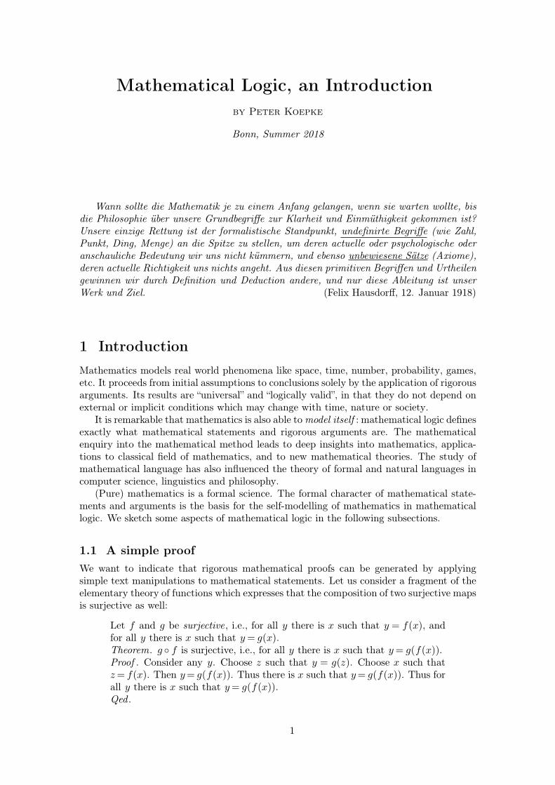
Wann sollte die Mathematik je zu einem Anfang gelangen, wenn sie warten wollte, bisdie Philosophie über unsere Grundbegriffe zur Klarheit und Einmüthigkeit gekommen ist?Unsere einzige Rettung ist der formalistische Standpunkt, undefinirte Begriffe (wie Zahl,Punkt, Ding, Menge) an die Spitze zu stellen, um deren actuelle oder psychologische oderanschauliche Bedeutung wir uns nicht kümmern, und ebenso unbewiesene Sätze (Axiome),deren actuelle Richtigkeit uns nichts angeht. Aus diesen primitiven Begriffen und Urtheilengewinnen wir durch Definition und Deduction andere, und nur diese Ableitung ist unserWerk und Ziel. (Felix Hausdorff, 12. Januar 1918)
1 Introduction
Mathematics models real world phenomena like space, time, number, probability, games,etc. It proceeds from initial assumptions to conclusions solely by the application of rigorousarguments. Its results are “universal” and “logically valid”, in that they do not depend onexternal or implicit conditions which may change with time, nature or society.
It is remarkable that mathematics is also able tomodel itself : mathematical logic definesexactly what mathematical statements and rigorous arguments are. The mathematicalenquiry into the mathematical method leads to deep insights into mathematics, applica-tions to classical field of mathematics, and to new mathematical theories. The study ofmathematical language has also influenced the theory of formal and natural languages incomputer science, linguistics and philosophy.
(Pure) mathematics is a formal science. The formal character of mathematical state-ments and arguments is the basis for the self-modelling of mathematics in mathematicallogic. We sketch some aspects of mathematical logic in the following subsections.
1.1 A simple proof
We want to indicate that rigorous mathematical proofs can be generated by applyingsimple text manipulations to mathematical statements. Let us consider a fragment of theelementary theory of functions which expresses that the composition of two surjective mapsis surjective as well:
Let f and g be surjective, i.e., for all y there is x such that y = f(x), andfor all y there is x such that y= g(x).Theorem. g ◦ f is surjective, i.e., for all y there is x such that y= g(f(x)).Proof . Consider any y. Choose z such that y = g(z). Choose x such thatz= f(x). Then y= g(f(x)). Thus there is x such that y= g(f(x)). Thus forall y there is x such that y= g(f(x)).Qed .
1
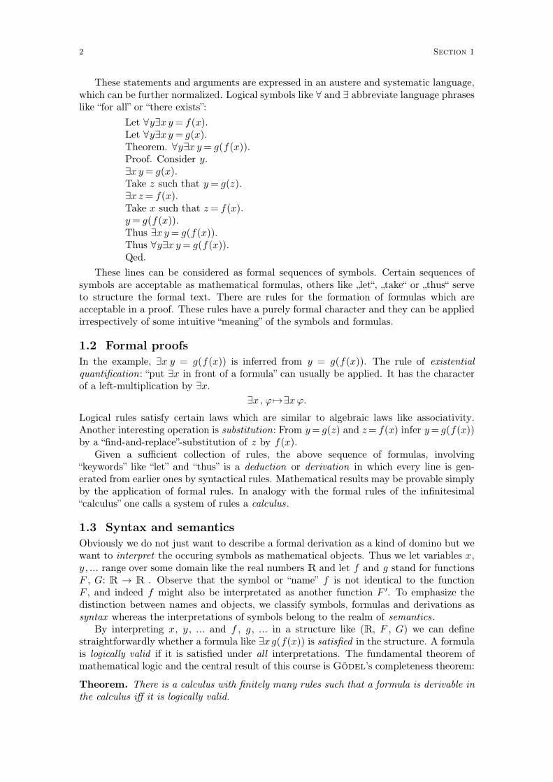
These statements and arguments are expressed in an austere and systematic language,which can be further normalized. Logical symbols like ∀ and ∃ abbreviate language phraseslike “for all” or “there exists”:
Let ∀y∃x y= f(x).Let ∀y∃x y= g(x).Theorem. ∀y∃x y= g(f(x)).Proof. Consider y.∃x y= g(x).Take z such that y= g(z).∃x z= f(x).Take x such that z= f(x).y= g(f(x)).Thus ∃x y= g(f(x)).Thus ∀y∃x y= g(f(x)).Qed.
These lines can be considered as formal sequences of symbols. Certain sequences ofsymbols are acceptable as mathematical formulas, others like „let“, „take“ or „thus“ serveto structure the formal text. There are rules for the formation of formulas which areacceptable in a proof. These rules have a purely formal character and they can be appliedirrespectively of some intuitive “meaning” of the symbols and formulas.
1.2 Formal proofs
In the example, ∃x y = g(f(x)) is inferred from y = g(f(x)). The rule of existentialquantification: “put ∃x in front of a formula” can usually be applied. It has the characterof a left-multiplication by ∃x.
∃x , ϕ 7→∃xϕ.
Logical rules satisfy certain laws which are similar to algebraic laws like associativity.Another interesting operation is substitution: From y= g(z) and z= f(x) infer y= g(f(x))by a “find-and-replace”-substitution of z by f(x).
Given a sufficient collection of rules, the above sequence of formulas, involving“keywords” like “let” and “thus” is a deduction or derivation in which every line is gen-erated from earlier ones by syntactical rules. Mathematical results may be provable simplyby the application of formal rules. In analogy with the formal rules of the infinitesimal“calculus” one calls a system of rules a calculus.
1.3 Syntax and semantics
Obviously we do not just want to describe a formal derivation as a kind of domino but wewant to interpret the occuring symbols as mathematical objects. Thus we let variables x,y, ... range over some domain like the real numbers R and let f and g stand for functionsF , G: R → R . Observe that the symbol or “name” f is not identical to the functionF , and indeed f might also be interpretated as another function F ′. To emphasize thedistinction between names and objects, we classify symbols, formulas and derivations assyntax whereas the interpretations of symbols belong to the realm of semantics .
By interpreting x, y, ... and f , g, ... in a structure like (R, F , G) we can definestraightforwardly whether a formula like ∃xg(f(x)) is satisfied in the structure. A formulais logically valid if it is satisfied under all interpretations. The fundamental theorem ofmathematical logic and the central result of this course is Gödel’s completeness theorem:
Theorem. There is a calculus with finitely many rules such that a formula is derivable inthe calculus iff it is logically valid.
2 Section 1
1.4 Object theory and meta theory
We shall use the common, informal mathematical language to express properties of aformal mathematical language. The formal language forms the object theory of our studies,the informal mathematical language is the “higher” or meta theory of mathematical logic.There will be strong parallels between object and meta theory which say that the modellingis faithful.
1.5 Set theory
In modern mathematics notions can usually be reduced to set theory: non-negative integerscorrespond to cardinalities of finite sets, integers can be obtained via pairs of non-neg-ative integers, rational numbers via pairs of integers, and real numbers via subsets ofthe rationals, etc. Geometric notions can be defined from real numbers using analyticgeometry: a point is a pair of real numbers, a line is a set of points, etc. It is remarkablethat the basic set theoretical axioms can be formulated in the logical language indicatedabove. So mathematics may be understood abstractly as
Mathematics = (first-order) logic + set theory.
Note that we only propose this as a reasonable abstract viewpoint corresponding to thelogical analysis of mathematics. This perspective leaves out many important aspects likethe applicability, intuitiveness and beauty of mathematics.
1.6 Set theory as meta theory
Our meta theory will be informal using the common notions of set, function, relation,natural, rational, real numbers, finite, infinite etc. We shall work informally but with aview towards possible formalization. Since we shall be interested in a weak theory able tocarry out logical syntax, we shall attempt to
not use the existence of infinite sets in syntactical considerations .
On the other hand the standard semantics requires infinite structures like the sets Nor R of numbers and we shall
use the existence of infinite sets in semantical considerations.
There will be exceptions to these rules where syntax and semantics merge like in theconstruction of structures out of infinite sets of terms.
In set theory, one usually distinguishes between sets and classes . A class is a collection{x| ϕ(x)} of objects x which satisfy some property ϕ . The axioms of set theory determinewhich of these classes are sets, i.e., can be taken as objects themselves.
1.7 Circularity
We shall use sets as symbols which can then be used to formulate the axioms of set theory.We shall prove theorems about proofs. This kind of circularity seems to be unavoidable incomprehensive foundational science: linguistics has to talk about language, brain researchhas to be carried out by brains. Circularity can lead to paradoxes like the liar’s paradox:“I am a liar”, or “this sentence is false”. Circularity poses many problems and seems toundermine the value of foundational theories. We suggest that the reader takes a naivestandpoint in these matters: there are sets and proofs which are just as obvious as naturalnumbers. Then theories are formed which abstractly describe the naive objects.
Introduction 3
A closer analysis of circularity in logic leads to the famous incompleteness theorems ofGödel:
Theorem. Formal theories which are strong enough to “formalize themselves” are notcomplete, i.e., there are statements such that neither it nor its negation can be proved inthat theory. Moreover such theories cannot prove their own consistency.
These results, besides their initial mathematical meaning, had a tremendous impact onthe theory of knowledge outside mathematics, e.g., in philosophy, psychology, linguistics.
2 The Syntax of first-order logic: Symbols, terms, andformulas
The art of free society consists firstin the maintenance of the symboliccode.
A. N. Whitehead
Formal mathematical statements will be finite sequences of symbols, just like ordinarysentences are sequences of alphabetic letters. These sequences can be studied mathemat-ically. We shall treat sequences as mathematical objects, similar to numbers or vectors.
The study of the formal properties of symbols, words, sentence,... is called syntax .Syntax will later be related to the “meaning” of symbolic material, its semantics. Theinterplay between syntax and semantics is at the core of logic. A strong logic is able topresent interesting semantic properties, i.e., properties of interesting mathematical struc-ture, already in its syntax.
We build the formal language with formulas like ∀y∃x y = g(f(x)) recursively fromatomic building blocks.
2.1 Symbols
Man muß jederzeit an Stellevon ’Punkte, Geraden, Ebenen’,’Tische, Stühle, Bierseidel’ sagenkönnen”.Quote ascribed to David Hilbert
A symbol has some basic information about its role within larger contexts like wordsand sentences. E.g., the symbol 6 is usually used to stand for a binary relation. So welet symbols include information on its function, like denoting a “relation”, together withfurther details, like “binary”.
Definition 1. The basic symbols of first-order logic are
a) ≡ for equality,
b) ¬,→,⊥ for the logical operations of negation, implication and the truth value false,
c) ∀ for universal quantification,
d) ( and ) for auxiliary bracketing.
e) variables vn for n∈N.
Let Var= {vn|n∈N} be the class of variables and let S0 be the class of basic symbols.
4 Section 2
There is a sufficiently rich class of relation symbols. Every relation symbol R possessesan arity which is a natural number. 1-ary relation symbols are called unary, 2-ary relationsymbols are called binary. A 0-ary relation symbol is also called a propositional constant(symbol).
Moreover there is a sufficiently rich class of function symbols. Every function symbolf possesses an arity which is a natural number. A 0-ary function symbol is also called aconstant (symbol)l.
We assume that the basic symbols, the relation symbols, and the function symbols areall pairwise distinct.
A symbol class or a language is a class of relation symbols and function symbols.
An n-ary relation symbol is intended to denote an n-ary relation; an n-ary functionsymbol is intended to denote an n-ary function in some structure. A symbol class is alsocalled a type because it describes the type of structures which will later interpret thesymbols. We shall denote variables by letters like x, y, z , ..., relation symbols by P , Q,
R, ..., functions symbols by f , g,h, ... and constant symbols by c, c0, c1, ... We shall also useother typographical symbols in line with standard mathematical practice. A symbol like<, e.g., usually denotes a binary relation, and we could assume for definiteness that thereis some fixed formalization of < like <=(1, 999, 2), where 1 indicates a relation (symbol),999 is the “name” of the symbol, and 2 is its arity. Instead of the arbitrary 999 one couldalso take the number of < in some typographical coding system like unicode; there < iscoded by the decimal number 60 and we could set <= (1, 60, 2).
Example 2. The language of group theory is the language
SGr= {◦, e},
where ◦ is a binary function symbol and e is a constant (symbol). Again one could bedefinite about the coding of symbols and set SGr = {(2, 9900, 2), (2, 101, 0)}, followingunicode, but we shall not care about such detail. As usual in algebra, one also uses anextended language of group theory
SGr′= {◦,−1, e}
to describe groups, where −1 is a unary function symbol (for forming inverses).
2.2 Words
Words:A letter and a letter on a stringWill hold forever humanity spell-boundThe Real Group
Definition 3. Let S be a language. A word over S is a finite sequence
w= s0s1...sn−1
where each si is an element of S0∪S. The number n is called the length of w: length(w)=n . The empty sequence ∅ is also called the empty word. Let S∗ be the class of all wordsover S.
Definition 4. If w= s0s1...sm−1 and w ′= s0′s1
′ ...sn−1′ are words over S then
w
˘w ′= s0s1...sm−1s0
′s1′ ...sn−1
′
is the concatenation of w and w ′. We also write ww ′ instead of w˘w ′.
The Syntax of first-order logic: Symbols, terms, and formulas 5
Exercise 1. The operation of concatenation satisfies some canonical laws:
a)˘is associative: (ww ′)w ′′=w(w ′w ′′).
b) ∅ is a neutral element for
˘: ∅w=w∅=w.
c)˘satisfies cancelation: if uw= u′w then u= u′; if wu=wu′ then u= u′.
2.3 Terms
Fix a language S.
Definition 5. The class TS of all S-terms is the smallest subclass of S∗ such that
a) x∈TS for all variables x;
b) ft0...tn−1 ∈ TS for all n ∈ N, all n-ary function symbols f ∈ S, and all t0, ...,
tn−1∈ TS.
Terms are written in Polish notation, meaning that function symbols come first and
that no brackets are needed. Indeed, terms in TS have unique readings according to thefollowing
Lemma 6. For every term t∈TS exactly one of the following holds:
a) t is a variable;
b) there is a uniquely defined function symbol f ∈ S and a uniquely defined sequencet0, ..., tn−1∈T S of terms, where f is n-ary, such that t= ft0...tn−1 .
Proof. Exercise. �
Remark 7. Unique readability is essential for working with terms. Therefore if this Lemmawould not hold one would have to alter the definition of terms.
Example 8. For the language SGr= {◦, e} of group theory, terms in TSGr look like
e, v0, v1, ..., ◦ee, ◦evm , ◦vm e , ◦ee , ◦e◦ee , ..., ◦vi ◦vj vk , ◦◦vi vj vk , ... .
In standard notation we would write ◦vi ◦vj vk as (vi ◦ (vj ◦ vk)) and ◦◦vi vj vk as=((vi◦vj)◦vk). Later, if the operation ◦ should be seen to be associative, one might “leaveout” some brackets.
Exercise 2. Show that every term t∈TSGr has odd length 2 n+1 where n is the number of ◦-symbolsin t.
2.4 Formulas
Definition 9. The class LS of all S-formulas is the smallest subclass of S∗ such that
a) ⊥∈LS (the false formula);
b) t0≡ t1∈LS for all S-terms t0, t1∈T S (equality);
c) Rt0...tn−1∈LS for all n-ary relation symbols R∈S and all S-terms t0, ..., tn−1∈TS
(relational formula);
d) ¬ϕ∈LS for all ϕ∈LS (negation);
e) (ϕ→ ψ)∈LS for all ϕ, ψ ∈LS (implication);
f ) ∀xϕ∈LS for all ϕ∈LS and all variables x (universalisation).
6 Section 2
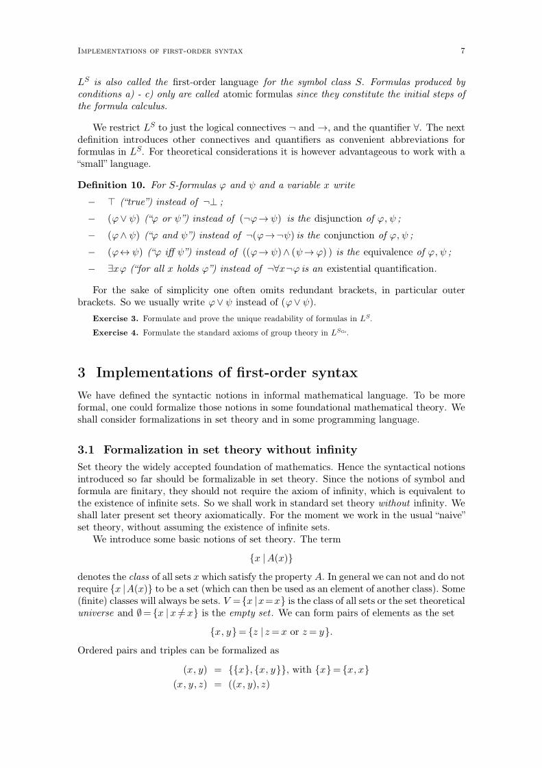
LS is also called the first-order language for the symbol class S. Formulas produced byconditions a) - c) only are called atomic formulas since they constitute the initial steps ofthe formula calculus.
We restrict LS to just the logical connectives ¬ and →, and the quantifier ∀. The nextdefinition introduces other connectives and quantifiers as convenient abbreviations forformulas in LS. For theoretical considerations it is however advantageous to work with a“small” language.
Definition 10. For S-formulas ϕ and ψ and a variable x write
− ⊤ (“true”) instead of ¬⊥ ;
− (ϕ∨ ψ) (“ϕ or ψ”) instead of (¬ϕ→ ψ) is the disjunction of ϕ, ψ ;
− (ϕ∧ ψ) (“ϕ and ψ”) instead of ¬(ϕ→¬ψ) is the conjunction of ϕ, ψ ;
− (ϕ↔ ψ) (“ϕ iff ψ”) instead of ((ϕ→ ψ)∧ (ψ→ ϕ) ) is the equivalence of ϕ, ψ ;
− ∃xϕ (“for all x holds ϕ”) instead of ¬∀x¬ϕ is an existential quantification.
For the sake of simplicity one often omits redundant brackets, in particular outerbrackets. So we usually write ϕ∨ ψ instead of (ϕ∨ ψ).
Exercise 3. Formulate and prove the unique readability of formulas in LS.
Exercise 4. Formulate the standard axioms of group theory in LSGr.
3 Implementations of first-order syntax
We have defined the syntactic notions in informal mathematical language. To be moreformal, one could formalize those notions in some foundational mathematical theory. Weshall consider formalizations in set theory and in some programming language.
3.1 Formalization in set theory without infinity
Set theory the widely accepted foundation of mathematics. Hence the syntactical notionsintroduced so far should be formalizable in set theory. Since the notions of symbol andformula are finitary, they should not require the axiom of infinity, which is equivalent tothe existence of infinite sets. So we shall work in standard set theory without infinity. Weshall later present set theory axiomatically. For the moment we work in the usual “naive”set theory, without assuming the existence of infinite sets.
We introduce some basic notions of set theory. The term
{x |A(x)}
denotes the class of all sets x which satisfy the property A. In general we can not and do notrequire {x |A(x)} to be a set (which can then be used as an element of another class). Some(finite) classes will always be sets. V ={x |x=x} is the class of all sets or the set theoreticaluniverse and ∅= {x | x=/ x} is the empty set . We can form pairs of elements as the set
{x, y}= {z | z= x or z= y}.
Ordered pairs and triples can be formalized as
(x, y) = {{x}, {x, y}}, with {x}= {x, x}
(x, y, z) = ((x, y), z)
Implementations of first-order syntax 7
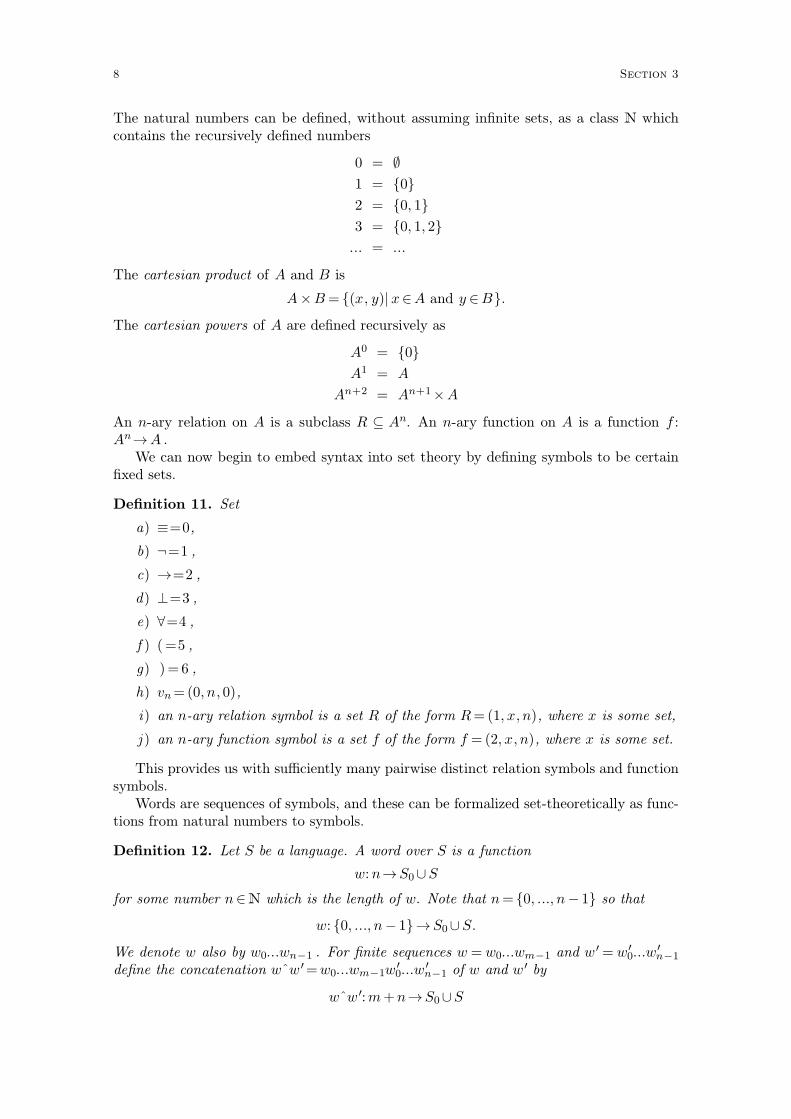
The natural numbers can be defined, without assuming infinite sets, as a class N whichcontains the recursively defined numbers
0 = ∅
1 = {0}
2 = {0, 1}
3 = {0, 1, 2}
... = ...
The cartesian product of A and B is
A×B= {(x, y)| x∈A and y ∈B}.
The cartesian powers of A are defined recursively as
A0 = {0}
A1 = A
An+2 = An+1×A
An n-ary relation on A is a subclass R ⊆ An. An n-ary function on A is a function f :An→A .
We can now begin to embed syntax into set theory by defining symbols to be certainfixed sets.
Definition 11. Set
a) ≡=0,
b) ¬=1 ,
c) →=2 ,
d) ⊥=3 ,
e) ∀=4 ,
f ) (=5 ,
g) )= 6 ,
h) vn=(0, n, 0),
i) an n-ary relation symbol is a set R of the form R= (1, x, n), where x is some set,
j ) an n-ary function symbol is a set f of the form f = (2, x, n), where x is some set.
This provides us with sufficiently many pairwise distinct relation symbols and functionsymbols.
Words are sequences of symbols, and these can be formalized set-theoretically as func-tions from natural numbers to symbols.
Definition 12. Let S be a language. A word over S is a function
w:n→S0∪S
for some number n∈N which is the length of w. Note that n= {0, ..., n− 1} so that
w: {0, ..., n− 1}→S0∪S.
We denote w also by w0...wn−1 . For finite sequences w = w0...wm−1 and w ′ = w0′ ...wn−1
′
define the concatenation wˆw ′=w0...wm−1w0′ ...wn−1
′ of w and w ′ by
wˆw ′:m+n→S0∪S
8 Section 3
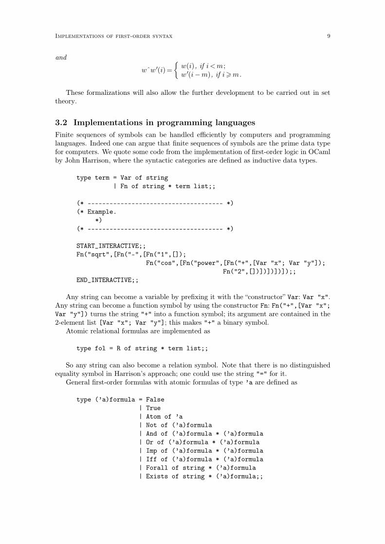
and
wˆw ′(i)=
�w(i), if i <m ;w ′(i−m), if i>m.
These formalizations will also allow the further development to be carried out in settheory.
3.2 Implementations in programming languages
Finite sequences of symbols can be handled efficiently by computers and programminglanguages. Indeed one can argue that finite sequences of symbols are the prime data typefor computers. We quote some code from the implementation of first-order logic in OCamlby John Harrison, where the syntactic categories are defined as inductive data types.
type term = Var of string
| Fn of string * term list;;
(* ––––––––––––––––––––––––––––––––––––- *)
(* Example.
*)
(* ––––––––––––––––––––––––––––––––––––- *)
START_INTERACTIVE;;
Fn("sqrt",[Fn("-",[Fn("1",[]);
Fn("cos",[Fn("power",[Fn("+",[Var "x"; Var "y"]);
Fn("2",[])])])])]);;
END_INTERACTIVE;;
Any string can become a variable by prefixing it with the “constructor” Var: Var "x".Any string can become a function symbol by using the constructor Fn: Fn("+",[Var "x";
Var "y"]) turns the string "+" into a function symbol; its argument are contained in the2-element list [Var "x"; Var "y"]; this makes "+" a binary symbol.
Atomic relational formulas are implemented as
type fol = R of string * term list;;
So any string can also become a relation symbol. Note that there is no distinguishedequality symbol in Harrison’s approach; one could use the string "=" for it.
General first-order formulas with atomic formulas of type ’a are defined as
type (’a)formula = False
| True
| Atom of ’a
| Not of (’a)formula
| And of (’a)formula * (’a)formula
| Or of (’a)formula * (’a)formula
| Imp of (’a)formula * (’a)formula
| Iff of (’a)formula * (’a)formula
| Forall of string * (’a)formula
| Exists of string * (’a)formula;;
Implementations of first-order syntax 9
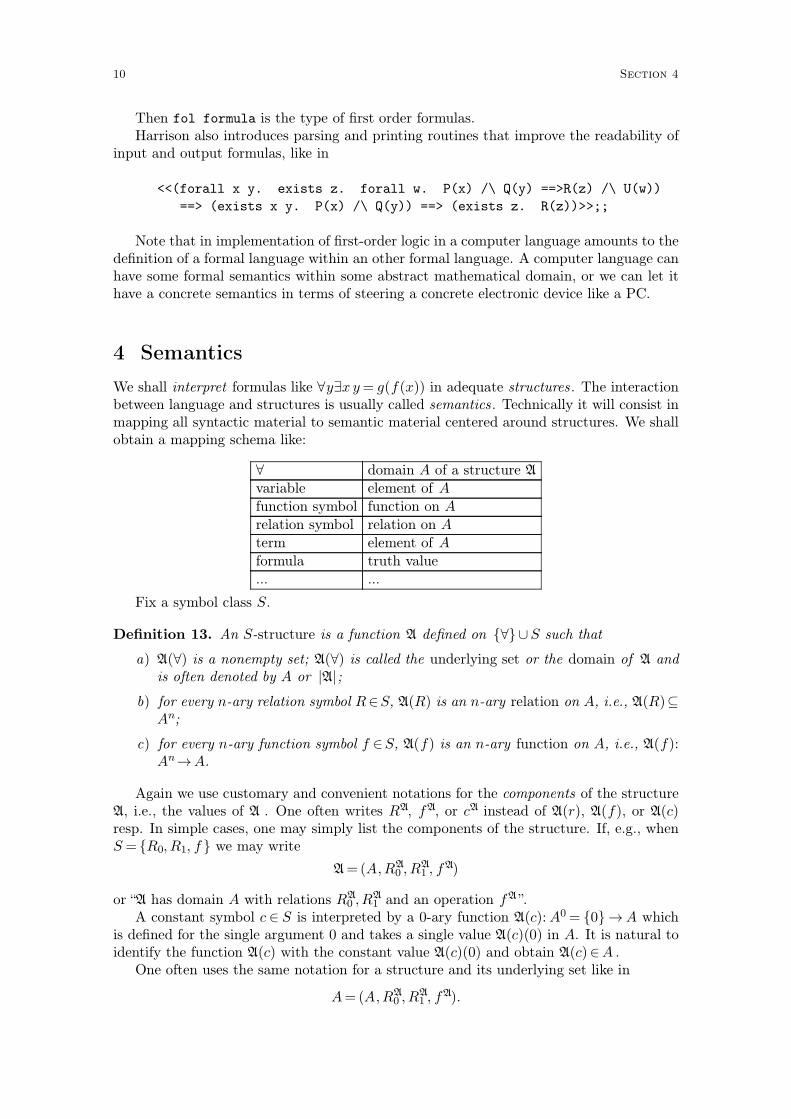
Then fol formula is the type of first order formulas.Harrison also introduces parsing and printing routines that improve the readability of
input and output formulas, like in
<<(forall x y. exists z. forall w. P(x) /\ Q(y) ==>R(z) /\ U(w))
==> (exists x y. P(x) /\ Q(y)) ==> (exists z. R(z))>>;;
Note that in implementation of first-order logic in a computer language amounts to thedefinition of a formal language within an other formal language. A computer language canhave some formal semantics within some abstract mathematical domain, or we can let ithave a concrete semantics in terms of steering a concrete electronic device like a PC.
4 Semantics
We shall interpret formulas like ∀y∃x y= g(f(x)) in adequate structures . The interactionbetween language and structures is usually called semantics . Technically it will consist inmapping all syntactic material to semantic material centered around structures. We shallobtain a mapping schema like:
∀ domain A of a structure A
variable element of A
function symbol function on A
relation symbol relation on A
term element of A
formula truth value
... ...
Fix a symbol class S.
Definition 13. An S-structure is a function A defined on {∀}∪S such that
a) A(∀) is a nonempty set; A(∀) is called the underlying set or the domain of A andis often denoted by A or |A|;
b) for every n-ary relation symbol R∈S, A(R) is an n-ary relation on A, i.e., A(R)⊆An;
c) for every n-ary function symbol f ∈S, A(f) is an n-ary function on A, i.e., A(f):An→A.
Again we use customary and convenient notations for the components of the structureA, i.e., the values of A . One often writes RA, fA, or cA instead of A(r), A(f), or A(c)resp. In simple cases, one may simply list the components of the structure. If, e.g., whenS= {R0, R1, f } we may write
A=(A,R0A, R1
A, fA)
or “A has domain A with relations R0A, R1
A and an operation fA ”.A constant symbol c ∈ S is interpreted by a 0-ary function A(c):A0= {0}→A which
is defined for the single argument 0 and takes a single value A(c)(0) in A. It is natural toidentify the function A(c) with the constant value A(c)(0) and obtain A(c)∈A .
One often uses the same notation for a structure and its underlying set like in
A= (A,R0A, R1
A, fA).
10 Section 4
This “overloading” of notation is common in mathematics (and in natural language). Usu-ally a human reader is readily able to detect and “disambiguate” ambiguities introduced bymultiple usage. There are techniques in computer science to deal with overloading, e.g., bytyping of notions. Another common overloading is given by a naive identification of syntaxand semantics, i.e., by writing
A=(A,R0, R1, f) instead of A= (A,R0A, R1
A, fA)
Since we are particularly interested in the interplay of syntax and semantics we shall tryto avoid this particular kind of overloading.
Example 14. Formalize the ordered field of reals R as follows. Define the language ofordered fields
SOF= {<,+, ·, 0, 1}.
Then define the SOF-structure R by
R(∀) = R
R(<)=<R = {(u, v)∈R2 |u<v}
R(+)=+R = {(u, v,w)∈R3 |u+ v=w}
R(·)= ·R = {(u, v,w)∈R3 |u · v=w}
R(0)= 0R = 0∈R
R(1)= 1R = 1∈R
This defines the standard structure R= (R, <R,+R, ·R, 0R, 1R).Observe that the symbols could in principle be interpreted in completely different, even
counterintuitive ways like
R′(∀) = N
R′(<) = {(u, v)∈N2 |u> v}
R′(+) = {(u, v, w)∈N3 |u · v=w}
R′(·) = {(u, v, w)∈N3 |u+ v=w}
R′(0) = 1
R′(1) = 0
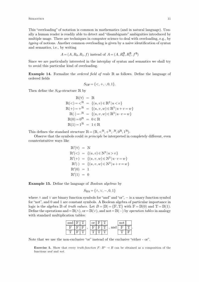
Example 15. Define the language of Boolean algebras by
SBA= {∧,∨,−, 0, 1}
where ∧ and ∨ are binary function symbols for “and” and “or”, − is a unary function symbolfor “not”, and 0 and 1 are constant symbols. A Boolean algebra of particular importance inlogic is the algebra B of truth values. Let B= |B|= {F,T} with F=B(0) and T=B(1).Define the operations and=B(∧), or=B(∨), and not=B(−) by operation tables in analogywith standard multiplication tables:
and F T
F F F
T F T
,or F T
F F T
T T T
, andnot
F T
T F
.
Note that we use the non-exclusive “or” instead of the exclusive “either - or”.
Exercise 5. Show that every truth-function F : Bn → B can be obtained as a composition of the
functions and and not .
Semantics 11

The notion of structure leads to derived definitions.
Definition 16. Let A be an S-structure and A′ be an S ′-structure. Then A is a reductof A′, or A′ is an expansion of A, if S ⊆S ′ and A′ ↾ ({∀}∪S)=A .
According to this definition, the additive group (R,+,0) of reals is a reduct of the field(R,+, ·, 0, 1).
Definition 17. Let A,B be S-structures. Then A is a substructure of B, A⊆B, if B
is a pointwise extension of A, i.e.,
a) A= |A|⊆ |B|;
b) for every n-ary relation symbol R∈S holds RA=RB∩An;
c) for every n-ary function symbol f ∈S holds fA= fB↾An.
Definition 18. Let A,B be S-structures and h: |A|→ |B|. Then h is a homomorphismfrom A into B, h:A→B, if
a) for every n-ary relation symbol R∈S and for every a0, ..., an−1∈A
RA(a0, ..., an−1) implies RB(h(a0), ..., h(an−1));
b) for every n-ary function symbol f ∈S and for every a0, ..., an−1∈A
fB(h(a0), ..., h(an−1))=h(fA(a0, ..., an−1)).
h is an embedding of A into B, h:A →֒B, if moreover
a) h is injective;
b) for every n-ary relation symbol R∈S and for every a0, ..., an−1∈A
RA(a0, ..., an−1) iff RB(h(a0), ..., h(an−1)).
If h is also bijective, it is called an isomorphism.
5 The satisfaction relation
“What is truth?” Pilate asked.John 18:38
An S-structure interprets the symbols in S. To interpret a formula in a structure, onealso has to interpret the (occuring) variables.
Definition 19. Let S be a language. An S-model is a function
M: {∀}∪S ∪Var→V
such that M ↾ {∀}∪S is an S-structure and for all n∈N holds M(vn)∈ |M|. M(vn) is theinterpretation or valuation of the variable vn in M.
It will be important to modify a model M at specific variables. For pairwise distinctvariables x0, ..., xr−1 and a0, ..., ar−1∈ |M| define
Ma0...ar−1
x0...xr−1=(M \ {(x0,A(x0)), ..., (xr−1,A(xr−1))})∪ {(x0, a0), ..., (xr−1, ar−1)}.
12 Section 5
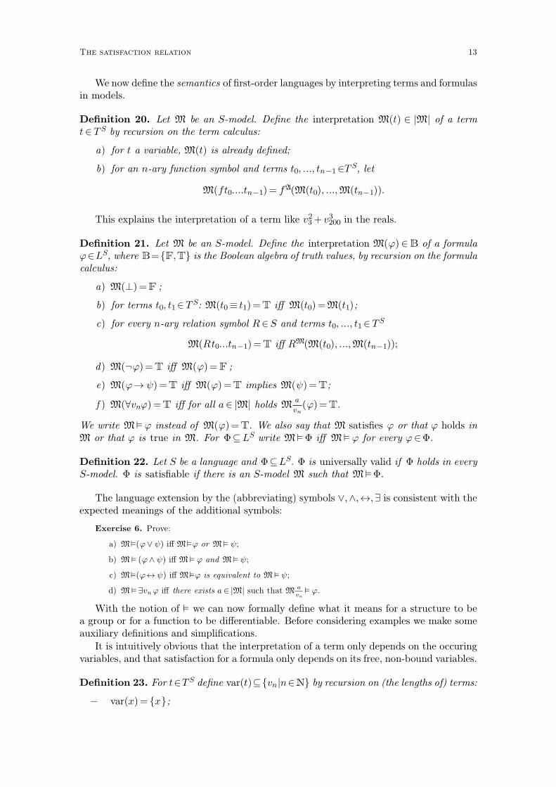
We now define the semantics of first-order languages by interpreting terms and formulasin models.
Definition 20. Let M be an S-model. Define the interpretation M(t) ∈ |M| of a termt∈ TS by recursion on the term calculus:
a) for t a variable, M(t) is already defined;
b) for an n-ary function symbol and terms t0, ..., tn−1∈T S, let
M(ft0....tn−1)= fA(M(t0), ...,M(tn−1)).
This explains the interpretation of a term like v32+ v200
3 in the reals.
Definition 21. Let M be an S-model. Define the interpretation M(ϕ)∈B of a formulaϕ∈LS, where B={F,T} is the Boolean algebra of truth values, by recursion on the formulacalculus:
a) M(⊥)=F ;
b) for terms t0, t1∈T S: M(t0≡ t1)=T iff M(t0)=M(t1);
c) for every n-ary relation symbol R∈S and terms t0, ..., t1∈ TS
M(Rt0...tn−1)=T iff RM(M(t0), ...,M(tn−1));
d) M(¬ϕ)=T iff M(ϕ)=F ;
e) M(ϕ→ ψ)=T iff M(ϕ)=T implies M(ψ)=T;
f ) M(∀vnϕ)=T iff for all a∈ |M| holds Ma
vn(ϕ)=T.
We write M� ϕ instead of M(ϕ)=T. We also say that M satisfies ϕ or that ϕ holds inM or that ϕ is true in M. For Φ⊆LS write M�Φ iff M� ϕ for every ϕ∈Φ.
Definition 22. Let S be a language and Φ⊆LS. Φ is universally valid if Φ holds in everyS-model. Φ is satisfiable if there is an S-model M such that M�Φ.
The language extension by the (abbreviating) symbols ∨,∧,↔,∃ is consistent with theexpected meanings of the additional symbols:
Exercise 6. Prove:
a) M�(ϕ∨ ψ) iff M�ϕ or M � ψ;
b) M � (ϕ∧ ψ) iff M � ϕ and M � ψ;
c) M�(ϕ↔ ψ) iff M�ϕ is equivalent to M � ψ;
d) M � ∃vnϕ iff there exists a∈ |M| such that Ma
vn
� ϕ.
With the notion of � we can now formally define what it means for a structure to bea group or for a function to be differentiable. Before considering examples we make someauxiliary definitions and simplifications.
It is intuitively obvious that the interpretation of a term only depends on the occuringvariables, and that satisfaction for a formula only depends on its free, non-bound variables.
Definition 23. For t∈TS define var(t)⊆{vn|n∈N} by recursion on (the lengths of) terms:
− var(x)= {x};
The satisfaction relation 13
− var(c)= ∅;
− var(ft0...tn−1)=S
i<nvar(ti).
Definition 24. Für ϕ∈LS define the set of free variables free(ϕ)⊆{vn|n∈N} by recursionon (the lengths of) formulas:
− free(t0≡ t1)= var(t0)∪ var(t1);
− free(Rt0...tn−1)= var( t0)∪ ...∪ var(tn−1);
− free(¬ϕ)= free(ϕ);
− free(ϕ→ ψ)= free(ϕ)∪ free(ψ).
− free(∀xϕ)= free(ϕ) \ {x}.
For Φ⊆LS define the class free(Φ) of free variables as
free(Φ)=[
ϕ∈Φ
free(ϕ) .
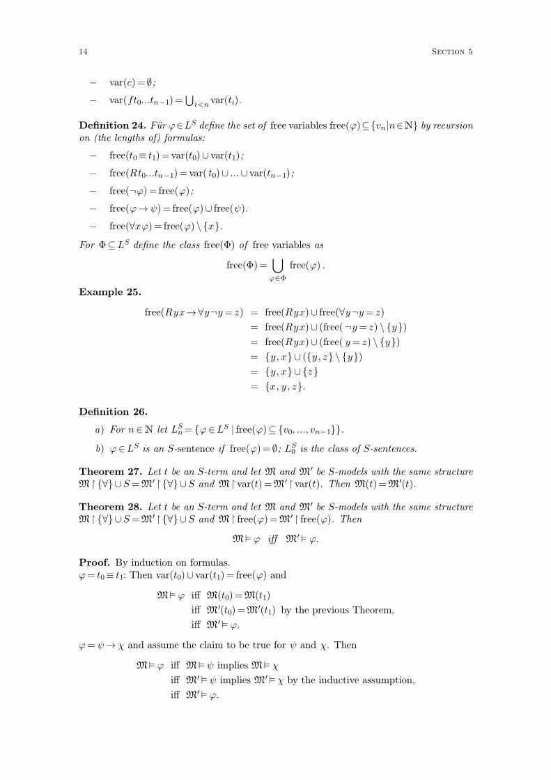
Example 25.
free(Ryx→∀y¬y= z) = free(Ryx)∪ free(∀y¬y= z)
= free(Ryx)∪ (free(¬y= z) \ {y})
= free(Ryx)∪ (free( y= z) \ {y})
= {y, x}∪ ({y, z} \ {y})
= {y, x}∪ {z}
= {x, y, z}.
Definition 26.
a) For n∈N let LnS= {ϕ∈LS | free(ϕ)⊆ {v0, ..., vn−1}}.
b) ϕ∈LS is an S-sentence if free(ϕ)= ∅; L0S is the class of S-sentences.
Theorem 27. Let t be an S-term and let M and M′ be S-models with the same structureM ↾ {∀}∪S=M′ ↾ {∀}∪S and M ↾ var(t)=M′ ↾ var(t). Then M(t)=M′(t).
Theorem 28. Let t be an S-term and let M and M′ be S-models with the same structureM ↾ {∀}∪S=M′ ↾ {∀}∪S and M ↾ free(ϕ)=M′ ↾ free(ϕ). Then
M� ϕ iff M′� ϕ.
Proof. By induction on formulas.ϕ= t0≡ t1: Then var(t0)∪ var(t1)= free(ϕ) and
M� ϕ iff M(t0)=M(t1)
iff M′(t0)=M′(t1) by the previous Theorem,
iff M′� ϕ.
ϕ= ψ→ χ and assume the claim to be true for ψ and χ. Then
M� ϕ iff M� ψ implies M� χ
iff M′� ψ implies M′� χ by the inductive assumption,
iff M′� ϕ.
14 Section 5
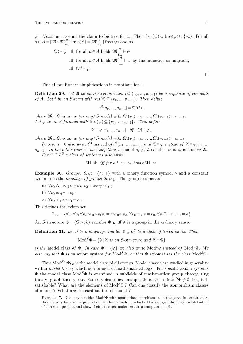
ϕ= ∀vnψ and assume the claim to be true for ψ. Then free(ψ)⊆ free(ϕ) ∪ {vn}. For alla∈A= |M|: M
a
vn↾ free(ψ)=M′ a
vn↾ free(ψ) and so
M� ϕ iff for all a∈A holds Ma
vn� ψ
iff for all a∈A holds M′ a
vn� ψ by the inductive assumption,
iff M′� ϕ.
�
This allows further simplifications in notations for �:
Definition 29. Let A be an S-structure and let (a0, ..., an−1) be a sequence of elementsof A. Let t be an S-term with var(t)⊆ {v0, ..., vn−1}. Then define
tA[a0, ..., an−1] =M(t),
where M⊇A is some (or any) S-model with M(v0)= a0 , ...,M(vn−1)= an−1.Let ϕ be an S-formula with free(ϕ)⊆ {v0, ..., vn−1}. Then define
A� ϕ[a0, ..., an−1] iff M� ϕ,
where M⊇A is some (or any) S-model with M(v0)= a0 , ...,M(vn−1)= an−1 .
In case n=0 also write tA instead of tA[a0, ..., an−1], and A� ϕ instead of A� ϕ[a0, ...,an−1]. In the latter case we also say: A is a model of ϕ, A satisfies ϕ or ϕ is true in A.
For Φ⊆L0S a class of sentences also write
A�Φ iff for all ϕ∈Φ holds :A� ϕ.
Example 30. Groups. SGr: ={◦, e} with a binary function symbol ◦ and a constantsymbol e is the language of groups theory . The group axioms are
a) ∀v0∀v1 ∀v2 ◦v0 ◦ v1v2≡◦◦v0v1v2 ;
b) ∀v0 ◦v0 e≡ v0 ;
c) ∀v0∃v1 ◦v0v1≡ e .
This defines the axiom set
ΦGr= {∀v0∀v1∀v2 ◦v0 ◦ v1v2≡◦◦v0v1v2, ∀v0 ◦v0 e≡ v0, ∀v0∃v1 ◦v0v1≡ e}.
An S-structure G= (G, ∗, k) satisfies ΦGr iff it is a group in the ordinary sense.
Definition 31. Let S be a language and let Φ⊆L0S be a class of S-sentences. Then
ModSΦ= {A |A is an S-structure and A�Φ}
is the model class of Φ. In case Φ = {ϕ} we also write ModSϕ instead of ModSΦ. We
also say that Φ is an axiom system for ModSΦ, or that Φ axiomatizes the class ModSΦ .
Thus ModSGrΦGr is the model class of all groups. Model classes are studied in generalitywithin model theory which is a branch of mathematical logic. For specific axiom systems
Φ the model class ModSΦ is examined in subfields of mathematics: group theory, ring
theory, graph theory, etc. Some typical questions questions are: is ModSΦ =/ ∅, i.e., is Φsatisfiable? What are the elements of ModSΦ ? Can one classify the isomorphism classesof models? What are the cardinalities of models?
Exercise 7. One may consider ModSΦ with appropriate morphisms as a category. In certain casesthis category has closure properties like closure under products. One can give the categorial definition
of cartesian product and show their existence under certain assumptions on Φ .
The satisfaction relation 15
6 Logical implication and propositional connectives
The design of the following treatiseis to investigate the fundamentallaws of those operations of the mindby which reasoning is performed; togive expression to them in the sym-bolical language of a Calculus, andupon this foundation to establishthe science of Logic and constructits method.George Boole, The Laws ofThought
Definition 32. For a symbol class S and Φ ⊆ LS and ϕ ∈ LS define that Φ (logically)implies ϕ (Φ� ϕ) iff every S-model I�Φ is also a model of ϕ.
Note that logical implication � is a relation between syntactical entities which is definedvia the semantic notion of interpretation. The relation Φ� ? can be viewed as the centralrelation in modern axiomatic mathematics: given the assumptions Φ what do they imply?The � -relation is usually verified by mathematical proofs. These proofs seem to refer tothe exploration of some domain of mathematical objects and, in practice, require particularmathematical skills and ingenuity.
We will however show that the logical implication � satisfies certain simple syntacticallaws. These laws correspond to ordinary proof methods but are purely formal. Amazingly afinite list of methods will (in principle) suffice for all mathematical proofs. This is Gödel’scompleteness theorem that we shall prove later.
Theorem 33. Let S be a language, t∈TS, ϕ, ψ ∈LS, and Γ,Φ⊆LS. Then
a) (Monotonicity) If Γ⊆Φ and Γ� ϕ then Φ� ϕ.
b) (Assumption property) If ϕ∈Γ then Γ� ϕ.
c) (→-Introduction) If Γ∪ ϕ� ψ then Γ� (ϕ→ ψ).
d) (→-Elimination) If Γ� ϕ and Γ� (ϕ→ ψ) then Γ� ψ.
e) (⊥-Introduction) If Γ� ϕ and Γ�¬ϕ then Γ�⊥ .
f ) (⊥-Elimination) If Γ∪ {¬ϕ}�⊥ then Γ� ϕ.
g) (≡-Introduction) Γ� t≡ t .
Proof. f) Assume Γ∪ {¬ϕ}�⊥ . Consider an S-model with M�Γ. Assume that M� ϕ.Then M � ¬ϕ . M � Γ ∪ {¬ϕ}, and by assumption, M �⊥ . But by the definition of thesatisfaction relation, this is false. Thus M� ϕ . Thus Γ� ϕ . �
Exercise 8. There are similar rules for the introduction and elimination of junctors like ∧ and ∨ that
we have introduced as abbreviations:
a) (∧-Introduction) If Γ� ϕ and Γ� ψ then Γ� ϕ∧ ψ.
b) (∧-Elimination) If Γ� ϕ∧ ψ then Γ� ϕ and Γ� ψ.
c) (∨-Introduction) If Γ� ϕ then Γ� ϕ∨ ψ and Γ� ψ ∨ ϕ.
d) (∨-Elimination) If Γ� ϕ∨ ψ and Γ⊢¬ϕ then Γ� ψ.
7 Substitution and term rules
To prove further rules for equality and quantification, we first have to consider the substi-tution of terms in formulas.
16 Section 7
Definition 34. For a term s∈TS, pairwise distinct variables x0, ..., xr−1 and terms t0, ...,tr−1∈ TS define the (simultaneous) substitution
st0....tr−1
x0...xr−1
of t0, ..., tr−1 for x0, ..., xr−1 by recursion:
a) xt0....tr−1
x0...xr−1=
�
x, if x=/ x0, ..., x=/ xr−1
ti , if x= xifor all variables x;
b) (fs0...sn−1)t0....tr−1
x0...xr−1= fs0
t0....tr−1
x0...xr−1...sn−1
t0....tr−1
x0...xr−1for all n-ary function symbols
f ∈S .
Note that the simultaneous substitution
st0....tr−1
x0...xr−1
is in general different from a successive substitution
st0x0
t1x1
...tr−1
xr−1
which depends on the order of substitution. E.g., xyx
xy= y, x
y
x
x
y= y
x
y= x and
xx
y
y
x= x
y
x= y.
Definition 35. For a formula ϕ ∈ LS, pairwise distinct variables x0, ..., xr−1 and termst0, ..., tr−1∈T S define the (simultaneous) substitution
ϕt0....tr−1
x0...xr−1
of t0, ..., tr−1 for x0, ..., xr−1 by recursion:
a) (s0≡ s1)t0....tr−1
x0...xr−1=s0
t0....tr−1
x0...xr−1≡ s1
t0....tr−1
x0...xr−1for all terms s0, s1∈TS;
b) (Rs0...sn−1)t0....tr−1
x0...xr−1=Rs0
t0....tr−1
x0...xr−1...sn−1
t0....tr−1
x0...xr−1for all n-ary relation symbols
R∈ s and terms s0, ..., sn−1∈T S;
c) (¬ϕ)t0....tr−1
x0...xr−1=¬(ϕ
t0....tr−1
x0...xr−1);
d) (ϕ→ ψ)t0....tr−1
x0...xr−1= (ϕ
t0....tr−1
x0...xr−1→ψ
t0....tr−1
x0...xr−1);
e) for (∀xϕ)t0....tr−1
x0...xr−1we proceed in two steps: let xi0, ..., xis−1
with i0 < ... < is−1 be
exactly those xi which are “relevant” for the substitution, i.e., xi ∈ free(∀xϕ) andxi=/ ti .
− if x does not occur in ti0, ...., tis−1, then set
(∀xϕ)t0....tr−1
x0...xr−1= ∀x (ϕ
ti0....tis−1
xi0...xis−1
).
− if x does occur in ti0, ...., tis−1, then let k ∈N minimal such that vk does not
occur in ϕ, ti0, ...., tis−1and set
(∀xϕ)t0....tr−1
x0...xr−1=∀vk (ϕ
ti0....tis−1vk
xi0...xis−1x).
Substitution and term rules 17
The following substitution theorem shows that syntactic substitution correspondssemantically to a (simultaneous) modification of assignments by interpreted terms. Thedefinition of substitution was intended to make the substitution theorem true. There arevariants of the syntactical substitution which could also satisfy the substitution theorem.
Theorem 36. Consider an S-model M, pairwise distinct variables x0, ..., xr−1 and termst0, ..., tr−1∈T S.
a) If s∈T S is a term,
M(st0...tr−1
x0...xr−1)=M
M(t0)...M(tr−1)x0...xr−1
(s).
b) If ϕ∈LS is a formula,
M� ϕt0...tr−1
x0...xr−1iff M
M(t0)...M(tr−1)x0...xr−1
� ϕ.
Proof. By induction on the complexities of s and ϕ.a) Case 1 : s= x.Case 1.1 : x∈/ {x0, ..., xr−1}. Then
M(xt0...tr−1
x0...xr−1)=M(x)=M
M(t0)...M(tr−1)x0...xr−1
(x).
Case 1.2 : x=xi . Then
M(xt0...tr−1
x0...xr−1)=M(ti)=M
M(t0)...M(tr−1)x0...xr−1
(xi)=MM(t0)...M(tr−1)
x0...xr−1(x).
Case 2 : s = fs0...sn−1 where f ∈ S is an n-ary function symbol and the terms s0, ...,
sn−1∈ TS satisfy the theorem. Then
M((fs0...sn−1)t0...tr−1
x0...xr−1) = M(fs0
t0...tr−1
x0...xr−1...sn−1
t0...tr−1
x0...xr−1)
= M(f)(M(s0t0...tr−1
x0...xr−1), ...,M(sn−1
t0...tr−1
x0...xr−1))
= M(f)(MM(t0)...M(tr−1)
x0...xr−1(s0),
...,MM(t0)...M(tr−1)
x0...xr−1(sn−1))
= MM(t0)....M(tr−1)
x0...xr−1(fs0...sn−1).
Assuming that the substitution theorem is proved for terms, we proveb) Case 4 : ϕ=Rs0...sn−1 . Then
M� (Rs0...sn−1)t0....tr−1
x0...xr−1iff M�Rs0
t0....tr−1
x0...xr−1...sn−1
t0....tr−1
x0...xr−1
iff RM
�
M(s0t0....tr−1
x0...xr−1), ...,M(s1
t0....tr−1
x0...xr−1)
�
iff RM
�
MM(t0)....M(tr−1)
x0...xr−1(s0),
...,MM(t0)....M(tr−1)
x0...xr−1(sn−1)
�
iff MM(t0)....M(tr−1)
x0...xr−1�Rs0...sn−1
18 Section 7
Equations s0≡ s1 can be treated as a special case of the relational Case 4 . Propositionalcombinations of formulas by ⊥ , ¬ and → behave similar to terms; indeed formulas can beviewed as terms whose values are truth values. So we are left with universal quantification.
:Case 5 : ϕ=(∀xψ)
t0....tr−1
x0...xr−1, assuming that the theorem holds for ψ.
We proceed according to our definition of syntactic substitution. Let xi0, ..., xis−1with
i0< ... < is−1 be exactly those xi such that xi∈ free(∀xψ) and xi=/ ti . Since
MM(t0)...M(tr−1)
x0...xr−1� ϕ iff M
M(ti0)...M(tis−1)
xi0...xis−1
� ϕ ,
we can assume that (x0, ..., xr−1)= (xi0, ..., xis−1), i.e., every xi is free in ∀xψ, xi=/ x, and
xi=/ ti . Now follow the two cases in the definition of the substitution:
Case 5.1 : The variable x does not occur in t0, ...., tr−1 and
(∀xψ)t0....tr−1
x0...xr−1= ∀x (ψ
t0....tr−1
x0...xr−1).
M� (∀xψ)t0...tr−1
x0...xr−1iff M�∀x (ψ
t0...tr−1
x0...xr−1)
iff for all a∈M holds Ma
x� ψ
t0...tr−1
x0...xr−1
(definition of �)
iff for all a∈M holds
(Ma
x)M
a
x(t0)...M
a
x(tr−1)
x0...xr−1� ψ
(by the inductive hypothesis for ψ)
iff for all a∈M holds
(Ma
x)M(t0)...M(tr−1)
x0...xr−1� ψ
(since x does not occur in ti)
iff for all a∈M holds
MM(t0)...M(tr−1) a
x0...xr−1 x� ψ
(since x does not occur in x0, ..., xr−1)
iff for all a∈M holds
(MM(t0)...M(tr−1)
x0...xr−1)a
x� ψ
(by simple properties of assignments)
iff MM(t0)...M(tr−1)
x0...xr−1�∀xψ
Case 5.2 : The variable x occurs in t0, ...., tr−1 . Then
(∀xψ)t0....tr−1
x0...xr−1= ∀vk (ψ
t0....tr−1vkx0...xr−1
x),
Substitution and term rules 19
where k ∈N is minimal such that vk does not occur in ϕ, ti0, ...., tis−1.
M� (∀xψ)t0...tr−1
x0...xr−1iff M�∀vk (ψ
t0....tr−1vkx0...xr−1x
)
iff for all a∈M holds Ma
vk� ψ
t0...tr−1vkx0...xr−1x
iff for all a∈M holds
(Ma
vk)M
a
vk(t0)...M
a
vk(tr−1)M
a
vk(vk)
x0...xr−1 x� ψ
(inductive hypothesis for ψ)
iff for all a∈M holds
(Ma
x)M(t0)...M(tr−1)a
x0...xr−1x� ψ
(since vk does not occur in ti)
iff for all a∈M holds
MM(t0)...M(tr−1) a
x0...xr−1x� ψ
(since x is anyway sent to a)
iff for all a∈M holds
(MM(t0)...M(tr−1)
x0...xr−1)a
x� ψ
(by simple properties of assignments)
iff MM(t0)...M(tr−1)
x0...xr−1� ∀xψ
�
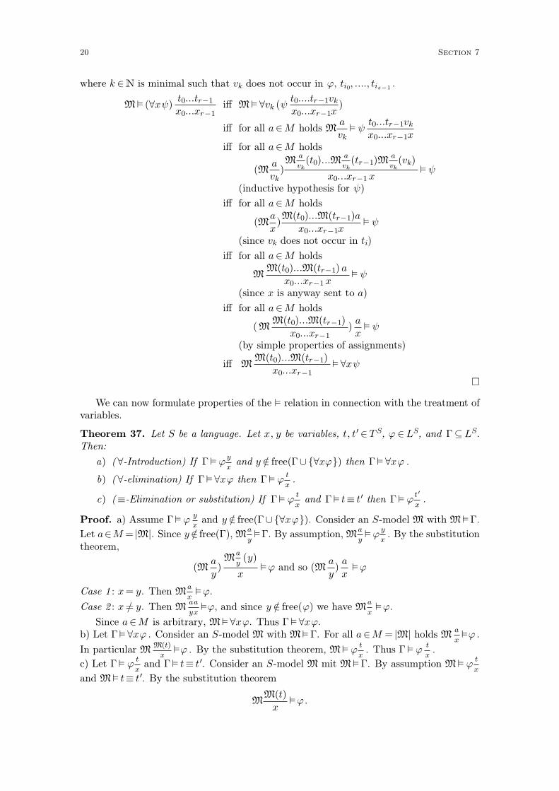
We can now formulate properties of the � relation in connection with the treatment ofvariables.
Theorem 37. Let S be a language. Let x, y be variables, t, t′∈ T S, ϕ ∈LS, and Γ⊆LS.Then:
a) (∀-Introduction) If Γ� ϕy
xand y ∈/ free(Γ∪ {∀xϕ}) then Γ� ∀xϕ .
b) (∀-elimination) If Γ� ∀xϕ then Γ� ϕt
x.
c) (≡-Elimination or substitution) If Γ� ϕt
xand Γ� t≡ t′ then Γ� ϕ
t′
x.
Proof. a) Assume Γ� ϕy
xand y ∈/ free(Γ∪ {∀xϕ}). Consider an S-model M with M�Γ.
Let a∈M = |M|. Since y∈/ free(Γ), Ma
y�Γ. By assumption, M
a
y�ϕ
y
x. By the substitution
theorem,
(Ma
y)M
a
y(y)
x�ϕ and so (M
a
y)a
x�ϕ
Case 1 : x= y. Then Ma
x�ϕ.
Case 2 : x=/ y. Then Maa
yx�ϕ, and since y ∈/ free(ϕ) we have M
a
x�ϕ.
Since a∈M is arbitrary, M�∀xϕ. Thus Γ�∀xϕ.b) Let Γ�∀xϕ . Consider an S-model M with M�Γ. For all a∈M = |M| holds M
a
x�ϕ .
In particular MM(t)
x�ϕ . By the substitution theorem, M� ϕ
t
x. Thus Γ� ϕ
t
x.
c) Let Γ� ϕt
xand Γ� t≡ t′. Consider an S-model M mit M�Γ. By assumption M� ϕ
t
x
and M� t≡ t′. By the substitution theorem
MM(t)
x�ϕ .
20 Section 7
Since M(t)=M(t′),
MM(t′)x
�ϕ
and again by the substitution theorem
M� ϕt′
x.
Thus Γ� ϕt′
x. �
Note that in proving these proof rules we have used corresponding forms of arguments inthe language of our discourse. This “circularity” was noted before and is a general feature informalizations of logic. A particularly important method of proof is the ∀-introduction: toprove a universal statement ∀xϕ it suffices to consider an “arbitrary but fixed” y and provethe claim for y . Formally this corresponds to using a “new” variable y ∈/ free(Γ∪ {∀xϕ}).
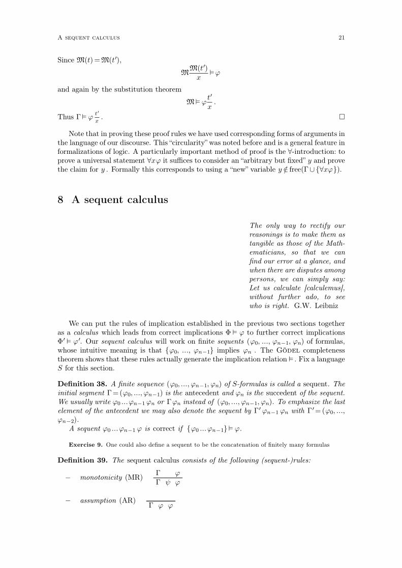
8 A sequent calculus
The only way to rectify ourreasonings is to make them astangible as those of the Math-ematicians, so that we canfind our error at a glance, andwhen there are disputes amongpersons, we can simply say:Let us calculate [calculemus],without further ado, to seewho is right. G.W. Leibniz
We can put the rules of implication established in the previous two sections togetheras a calculus which leads from correct implications Φ � ϕ to further correct implicationsΦ′ � ϕ′. Our sequent calculus will work on finite sequents (ϕ0, ..., ϕn−1, ϕn) of formulas,whose intuitive meaning is that {ϕ0, ..., ϕn−1} implies ϕn . The Gödel completenesstheorem shows that these rules actually generate the implication relation � . Fix a languageS for this section.
Definition 38. A finite sequence (ϕ0, ...,ϕn−1,ϕn) of S-formulas is called a sequent. Theinitial segment Γ=(ϕ0, ...,ϕn−1) is the antecedent and ϕn is the succedent of the sequent.We usually write ϕ0 ...ϕn−1ϕn or Γϕn instead of (ϕ0, ...,ϕn−1,ϕn). To emphasize the lastelement of the antecedent we may also denote the sequent by Γ′ ϕn−1 ϕn with Γ′=(ϕ0, ...,
ϕn−2).A sequent ϕ0 ...ϕn−1 ϕ is correct if {ϕ0 ...ϕn−1}� ϕ.
Exercise 9. One could also define a sequent to be the concatenation of finitely many formulas
Definition 39. The sequent calculus consists of the following (sequent-)rules:
− monotonicity (MR)Γ ϕ
Γ ψ ϕ
− assumption (AR)Γ ϕ ϕ
A sequent calculus 21
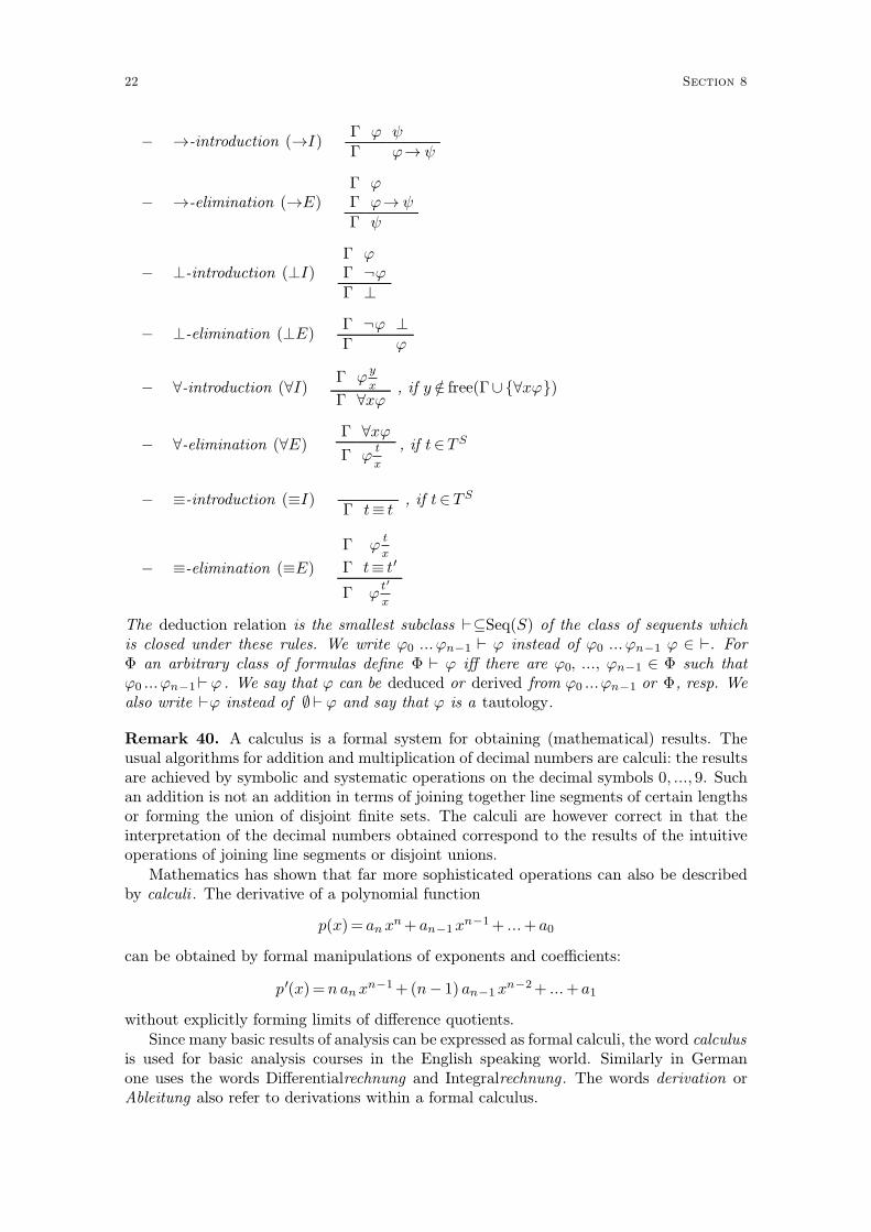
− →-introduction (→I)Γ ϕ ψ
Γ ϕ→ ψ
− →-elimination (→E)Γ ϕ
Γ ϕ→ ψ
Γ ψ
− ⊥-introduction (⊥I)Γ ϕ
Γ ¬ϕΓ ⊥
− ⊥-elimination (⊥E)Γ ¬ϕ ⊥Γ ϕ
− ∀-introduction (∀I)Γ ϕ
y
x
Γ ∀xϕ, if y ∈/ free(Γ∪ {∀xϕ})
− ∀-elimination (∀E)Γ ∀xϕ
Γ ϕt
x
, if t∈TS
− ≡-introduction (≡I)Γ t≡ t
, if t∈ TS
− ≡-elimination (≡E)
Γ ϕt
x
Γ t≡ t′
Γ ϕt′
x
The deduction relation is the smallest subclass ⊢⊆Seq(S) of the class of sequents whichis closed under these rules. We write ϕ0 ...ϕn−1 ⊢ ϕ instead of ϕ0 ...ϕn−1 ϕ ∈ ⊢. ForΦ an arbitrary class of formulas define Φ ⊢ ϕ iff there are ϕ0, ..., ϕn−1 ∈ Φ such thatϕ0 ...ϕn−1⊢ ϕ . We say that ϕ can be deduced or derived from ϕ0 ...ϕn−1 or Φ, resp. Wealso write ⊢ϕ instead of ∅ ⊢ ϕ and say that ϕ is a tautology.
Remark 40. A calculus is a formal system for obtaining (mathematical) results. Theusual algorithms for addition and multiplication of decimal numbers are calculi: the resultsare achieved by symbolic and systematic operations on the decimal symbols 0, ..., 9. Suchan addition is not an addition in terms of joining together line segments of certain lengthsor forming the union of disjoint finite sets. The calculi are however correct in that theinterpretation of the decimal numbers obtained correspond to the results of the intuitiveoperations of joining line segments or disjoint unions.
Mathematics has shown that far more sophisticated operations can also be describedby calculi . The derivative of a polynomial function
p(x)= anxn+ an−1x
n−1+ ...+ a0
can be obtained by formal manipulations of exponents and coefficients:
p′(x)=nanxn−1+(n− 1) an−1 x
n−2+ ...+ a1
without explicitly forming limits of difference quotients.Since many basic results of analysis can be expressed as formal calculi, the word calculus
is used for basic analysis courses in the English speaking world. Similarly in Germanone uses the words Differentialrechnung and Integralrechnung . The words derivation orAbleitung also refer to derivations within a formal calculus.
22 Section 8
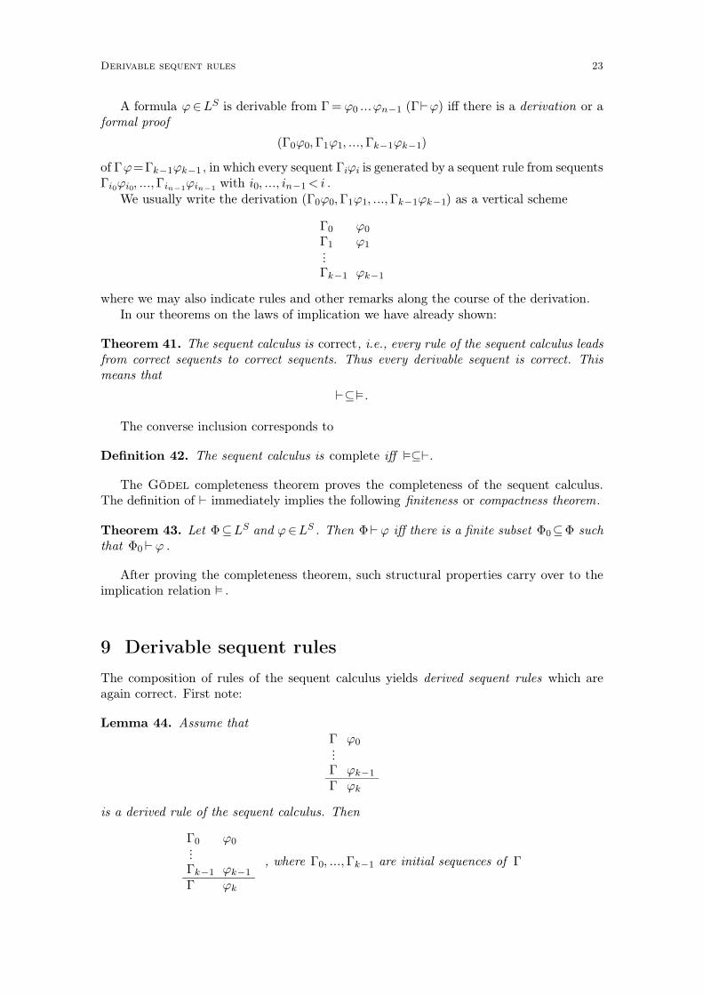
A formula ϕ∈LS is derivable from Γ= ϕ0 ...ϕn−1 (Γ⊢ϕ) iff there is a derivation or aformal proof
(Γ0ϕ0,Γ1ϕ1, ...,Γk−1ϕk−1)
of Γϕ=Γk−1ϕk−1 , in which every sequent Γiϕi is generated by a sequent rule from sequentsΓi0ϕi0, ...,Γin−1
ϕin−1with i0, ..., in−1<i .
We usually write the derivation (Γ0ϕ0,Γ1ϕ1, ...,Γk−1ϕk−1) as a vertical scheme
Γ0 ϕ0
Γ1 ϕ1···Γk−1 ϕk−1
where we may also indicate rules and other remarks along the course of the derivation.In our theorems on the laws of implication we have already shown:
Theorem 41. The sequent calculus is correct, i.e., every rule of the sequent calculus leadsfrom correct sequents to correct sequents. Thus every derivable sequent is correct. Thismeans that
⊢⊆�.
The converse inclusion corresponds to
Definition 42. The sequent calculus is complete iff �⊆⊢.
The Gödel completeness theorem proves the completeness of the sequent calculus.The definition of ⊢ immediately implies the following finiteness or compactness theorem.
Theorem 43. Let Φ⊆LS and ϕ∈LS . Then Φ⊢ ϕ iff there is a finite subset Φ0⊆Φ suchthat Φ0⊢ ϕ .
After proving the completeness theorem, such structural properties carry over to theimplication relation � .
9 Derivable sequent rules
The composition of rules of the sequent calculus yields derived sequent rules which areagain correct. First note:
Lemma 44. Assume thatΓ ϕ0···Γ ϕk−1
Γ ϕk
is a derived rule of the sequent calculus. Then
Γ0 ϕ0···Γk−1 ϕk−1
Γ ϕk
, where Γ0, ...,Γk−1 are initial sequences of Γ
Derivable sequent rules 23
is also a derived rule of the sequent calculus.
Proof. This follows immediately from iterated applications of the monotonicity rule. �
We now list several derived rules.
9.1 Auxiliary rules
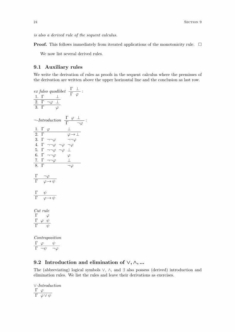
We write the derivation of rules as proofs in the sequent calculus where the premisses ofthe derivation are written above the upper horizontal line and the conclusion as last row.
ex falso quodlibetΓ ⊥Γ ϕ
:1. Γ ⊥2. Γ ¬ϕ ⊥3. Γ ϕ
¬-IntroductionΓ ϕ ⊥Γ ¬ϕ
:
1. Γ ϕ ⊥2. Γ ϕ→⊥3. Γ ¬¬ϕ ¬¬ϕ4. Γ ¬¬ϕ ¬ϕ ¬ϕ5. Γ ¬¬ϕ ¬ϕ ⊥6. Γ ¬¬ϕ ϕ
7. Γ ¬¬ϕ ⊥8. Γ ¬ϕ
Γ ¬ϕΓ ϕ→ ψ
Γ ψ
Γ ϕ→ ψ
Cut ruleΓ ϕ
Γ ϕ ψ
Γ ψ
ContrapositionΓ ϕ ψ
Γ ¬ψ ¬ϕ
9.2 Introduction and elimination of ∨,∧, ...
The (abbreviating) logical symbols ∨, ∧, and ∃ also possess (derived) introduction andelimination rules. We list the rules and leave their derivations as exercises.
∨-IntroductionΓ ϕ
Γ ϕ∨ ψ
24 Section 9
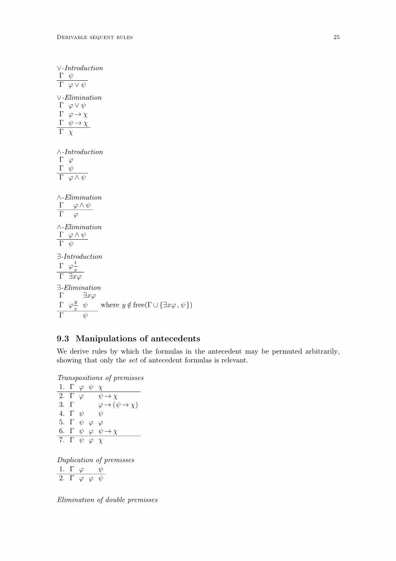
∨-IntroductionΓ ψ
Γ ϕ∨ ψ
∨-EliminationΓ ϕ∨ ψ
Γ ϕ→ χ
Γ ψ→ χ
Γ χ
∧-IntroductionΓ ϕ
Γ ψ
Γ ϕ∧ ψ
∧-EliminationΓ ϕ∧ ψ
Γ ϕ
∧-EliminationΓ ϕ∧ ψ
Γ ψ
∃-Introduction
Γ ϕt
x
Γ ∃xϕ
∃-EliminationΓ ∃xϕ
Γ ϕy
xψ where y ∈/ free(Γ∪ {∃xϕ , ψ})
Γ ψ
9.3 Manipulations of antecedents
We derive rules by which the formulas in the antecedent may be permuted arbitrarily,showing that only the set of antecedent formulas is relevant.
Transpositions of premisses1. Γ ϕ ψ χ
2. Γ ϕ ψ→ χ
3. Γ ϕ→ (ψ→ χ)4. Γ ψ ψ
5. Γ ψ ϕ ϕ
6. Γ ψ ϕ ψ→ χ
7. Γ ψ ϕ χ
Duplication of premisses1. Γ ϕ ψ
2. Γ ϕ ϕ ψ
Elimination of double premisses
Derivable sequent rules 25
1. Γ ϕ ϕ ψ
2. Γ ϕ ϕ→ ψ
3. Γ ϕ→ (ϕ→ ψ)4. Γ ϕ ϕ
5. Γ ϕ ψ
Iterated applications of these rules yield:
Lemma 45. Let ϕ0...ϕm−1 and ψ0...ψn−1 be antecedents such that
{ϕ0, ..., ϕm−1}= {ψ0, ..., ψn−1}
and χ∈LS. Thenϕ0 ... ϕm−1 χ
ψ0 ... ψn−1 χis a derived rule.
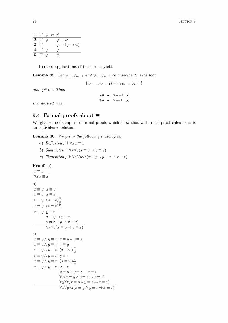
9.4 Formal proofs about ≡
We give some examples of formal proofs which show that within the proof calculus ≡ isan equivalence relation.
Lemma 46. We prove the following tautologies:
a) Reflexivity: ⊢∀xx≡x
b) Symmetry: ⊢∀x∀y(x≡ y→ y≡ x)
c) Transitivity: ⊢∀x∀y∀z(x≡ y ∧ y≡ z→x≡ z)
Proof. a)
x≡ x
∀xx≡x
b)
x≡ y x≡ y
x≡ y x≡ x
x≡ y (z≡x)x
z
x≡ y (z≡x)y
x
x≡ y y≡x
x≡ y→ y≡x
∀y(x≡ y→ y≡ x)
∀x∀y(x≡ y→ y≡x)
c)
x≡ y ∧ y≡ z x≡ y ∧ y≡ z
x≡ y ∧ y≡ z x≡ y
x≡ y ∧ y≡ z (x≡w)y
w
x≡ y ∧ y≡ z y≡ z
x≡ y ∧ y≡ z (x≡w)z
w
x≡ y ∧ y≡ z x≡ z
x≡ y ∧ y≡ z→ x≡ z
∀z(x≡ y ∧ y≡ z→x≡ z)∀y∀z(x≡ y ∧ y≡ z→ x≡ z)
∀x∀y∀z(x≡ y ∧ y≡ z→ x≡ z)
26 Section 9
�
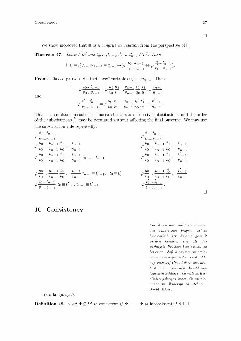
We show moreover that ≡ is a congruence relation from the perspective of ⊢.
Theorem 47. Let ϕ∈LS and t0, ..., tn−1, t0′ , ..., tn−1
′ ∈TS. Then
⊢ t0≡ t0′ ∧ ...∧ tn−1≡ tn−1
′ →(ϕt0...tn−1
v0...vn−1↔ ϕ
t0′ ...tn−1
′
v0...vn−1).
Proof. Choose pairwise distinct “new” variables u0, ..., un−1 . Then
ϕt0...tn−1
v0...vn−1=ϕ
u0v0
u1
v1...un−1
vn−1
t0u0
t1u1
...tn−1
un−1and
ϕt0′ ...tn−1
′
v0...vn−1=ϕ
u0v0
u1
v1...un−1
vn−1
t0′
u0
t1′
u1...
tn−1′
un−1.
Thus the simultaneous substitutions can be seen as successive substitutions, and the orderof the substitutions
ti
uimay be permuted without affecting the final outcome. We may use
the substitution rule repeatedly:
ϕt0...tn−1
v0...vn−1ϕ
t0...tn−1
v0...vn−1
ϕu0
v0...un−1
vn−1
t0u0
...tn−1
un−1ϕu0v0
...un−1
vn−1
t0u0
...tn−1
un−1
ϕu0
v0...un−1
vn−1
t0u0
...tn−1
un−1tn−1≡ tn−1
′ ϕu0v0
...un−1
vn−1
t0u0
...tn−1′
un−1···
ϕu0
v0...un−1
vn−1
t0u0
...tn−1
un−1tn−1≡ tn−1
′ ... t0≡ t0′ ϕ
u0v0
...un−1
vn−1
t0′
u0...
tn−1′
un−1
ϕt0...tn−1
v0...vn−1t0≡ t0
′ ... tn−1≡ tn−1′ ϕ
t0′ ...tn−1
′
v0...vn−1.
�
10 Consistency
Vor Allem aber möchte ich unter
den zahlreichen Fragen, welche
hinsichtlich der Axiome gestellt
werden können, dies als das
wichtigste Problem bezeichnen, zu
beweisen, daß dieselben unterein-
ander widerspruchslos sind, d.h.
daß man auf Grund derselben mit-
telst einer endlichen Anzahl von
logischen Schlüssen niemals zu Res-
ultaten gelangen kann, die mitein-
ander in Widerspruch stehen.
David Hilbert
Fix a language S.
Definition 48. A set Φ⊆LS is consistent if Φ�⊥ . Φ is inconsistent if Φ⊢⊥ .
Consistency 27
We prove some laws of consistency.
Lemma 49. Let Φ⊆LS and ϕ∈LS. Then
a) Φ is inconsistent iff there is ψ ∈LS such that Φ⊢ ψ and Φ⊢¬ψ.
b) Φ⊢ ϕ iff Φ∪ {¬ϕ} is inconsistent.
c) If Φ is consistent, then Φ∪ {ϕ} is consistent or Φ∪ {¬ϕ} is consistent (or both).
d) Let F be a family of consistent sets which is linearly ordered by inclusion, i.e., forall Φ,Ψ∈F holds Φ⊆Ψ or Ψ⊆Φ. Then
Φ∗=[
Φ∈F
Φ
is consistent.
Proof. a) Assume Φ⊢⊥ . Then by the ex falso rule, Φ⊢ ψ and Φ⊢¬ψ.Conversely assume that Φ ⊢ ψ and Φ ⊢ ¬ψ for some ψ ∈ LS. Then Φ ⊢ ⊥ by ⊥-
introduction.b) Assume Φ ⊢ ϕ . Take ϕ0, ..., ϕn−1 ∈ Φ such that ϕ0...ϕn−1 ⊢ ϕ . Then we can extenda derivation of ϕ0...ϕn−1⊢ ϕ as follows
ϕ0 ... ϕn−1 ϕ
ϕ0 ... ϕn−1 ¬ϕ ¬ϕϕ0 ... ϕn−1 ¬ϕ ⊥
and Φ∪ {¬ϕ} is inconsistent.Conversely assume that Φ∪ {¬ϕ}⊢⊥ and take ϕ0, ..., ϕn−1∈Φ such that ϕ0...ϕn−1¬
ϕ⊢⊥ . Then ϕ0...ϕn−1⊢ ϕ and Φ⊢ ϕ .c) Assume that Φ∪ {ϕ} and Φ∪ {¬ϕ} are inconsistent. Then there are ϕ0, ..., ϕn−1∈Φsuch that ϕ0...ϕn−1⊢ϕ and ϕ0...ϕn−1⊢¬ϕ. By the introduction rule for ⊥, ϕ0...ϕn−1⊢⊥.Thus Φ is inconsistent.d) Assume that Φ∗ is inconsistent. Take ϕ0, ..., ϕn−1 ∈ Φ∗ such that ϕ0 ...ϕn−1 ⊢ ⊥ .Take Φ0, ...Φn−1∈F such that ϕ0∈Φ0 , ..., ϕn−1∈Φn−1 . Since F is linearly ordered byinclusion there is Φ ∈ {Φ0, ...Φn−1} such that ϕ0, ..., ϕn−1 ∈ Φ. Then Φ is inconsistent,contradiction. �
The proof of the completeness theorem will be based on the relation between consist-ency and satisfiability.
Lemma 50. Assume that Φ⊆LS is satisfiable. Then Φ is consistent.
Proof. Assume that Φ ⊢ ⊥ . By the correctness of the sequent calculus, Φ �⊥ . Assumethat Φ is satisfiable and let M � Φ . Then M �⊥ . This contradicts the definition of thesatisfaction relation. Thus Φ is not satisfiable. �
We shall later show the converse of this Lemma, since:
Theorem 51. The sequent calculus is complete iff every consistent Φ⊆LS is satisfiable.
Proof. Assume that the sequent calculus is complete. Let Φ⊆LS be consistent, i.e., Φ�⊥ .By completeness, Φ�⊥ , and we can take an S-model M�Φ such that M�⊥ . Thus Φ issatisfiable.
Conversely, assume that every consistent Φ⊆LS is satisfiable. Assume Ψ�ψ . Assumefor a contradiction that Ψ � ψ . Then Ψ∪ {¬ψ} is consistent. By assumption there is anS-model M�Ψ∪ {¬ψ}. M�Ψ and M� ψ , which contradicts Ψ� ψ . Thus Ψ⊢ ψ . �
28 Section 10
11 Term models and Henkin sets
The following constructions will assume that the class of all terms of some
language is a set. In view of the previous lemma, we strive to construct interpretations forgiven sets Φ⊆LS of S-formulas. Since we are working in great generality and abstractness,the only material available for the construction of structures is the language LS itself. Weshall build a model out of S-terms.
Definition 52. Let S be a language and let Φ⊆LS be consistent. The term model TΦ ofΦ is the following S-model:
a) Define a relation ∼ on TS,
t0∼ t1 iff Φ⊢ t0≡ t1 .
∼ is an equivalence relation on TS.
b) For t∈T S let t̄ = {s∈TS |s∼ t} be the equivalence class of t.
c) The underlying set TΦ=TΦ(∀) of the term model is the set of ∼-equivalence classes
TΦ= {t̄ |t∈TS}.
d) For an n-ary relation symbol R∈S let RTΦ
on TΦ be defined by
( t̄0, ..., t̄n−1)∈RTΦ
iff Φ⊢Rt0...tn−1 .
e) For an n-ary function symbol f ∈S let fTΦ
on TΦ be defined by
fTΦ
( t̄0, ..., t̄n−1)= ft0...tn−1 .
f ) For n∈N define the variable interpretation TΦ(vn)= vn .
The term model is well-defined.
Lemma 53. In the previous construction the following holds:
a) ∼ is an equivalence relation on TS.
b) The definition of RTΦ
is independent of representatives.
c) The definition of fTΦ
is independent of representatives.
Proof. a) We derived the axioms of equivalence relations for ≡:
− ⊢∀xx≡x
− ⊢∀x∀y (x≡ y→ y≡x)
− ⊢∀x∀y∀z (x≡ y ∧ y≡ z→ x≡ z)
Consider t∈TS. Then ⊢t≡ t. Thus for all t∈TS holds t∼ t .Consider t0, t1∈ T S with t0∼ t1 . Then ⊢t0≡ t1 . Also ⊢t0≡ t1→ t1≡ t0 , ⊢t1≡ t0 , and
t1∼ t0 . Thus for all t0, t1∈TS with t0∼ t1 holds t1∼ t0 .The transitivity of ∼ follows similarly.
b) Let t̄0, ..., t̄n−1 ∈ TΦ, t̄0= s̄0, ..., t̄n−1= s̄n−1 and Φ ⊢Rt0...tn−1 . Then ⊢t0 ≡ s0 , ... ,⊢tn−1≡ sn−1 . Repeated applications of the substitution rule yield Φ⊢Rs0...sn−1 . HenceΦ ⊢Rt0...tn−1 implies Φ ⊢Rs0...sn−1 . By the symmetry of the argument, Φ ⊢Rt0...tn−1
iff Φ⊢Rs0...sn−1 .c) Let t̄0, ..., t̄n−1 ∈ TΦ and t̄0 = s̄0, ..., t̄n−1 = s̄n−1 . Then ⊢t0 ≡ s0 , ... , ⊢tn−1 ≡ sn−1 .Repeated applications of the substitution rule to ⊢ft0...tn−1≡ ft0...tn−1 yield
⊢ft0...tn−1≡ fs0...sn−1
Term models and Henkin sets 29
and ft0...tn−1= fs0...sn−1 . �
We aim to obtain TΦ � Φ. The initial cases of an induction over the complexity offormulas is given by
Theorem 54.
a) For terms t∈TS holds TΦ(t)= t̄.
b) For atomic formulas ϕ∈LS holds
TΦ� ϕ iff Φ⊢ ϕ.
Proof. a) By induction on the term calculus. The initial case t = vn is obvious by thedefinition of the term model. Now consider a term t = ft0...tn−1 with an n-ary functionsymbol f ∈S , and assume that the claim is true for t0, ..., tn−1 . Then
TΦ(ft0...tn−1) = fTΦ
(TΦ(t0), ...,TΦ(tn−1))
= fTΦ
(t0̄, ..., tn−1)
= ft0...tn−1 .
b) Let ϕ=Rt0...tn−1 with an n-ary relation symbol R∈S and t0, ..., tn−1∈ TS. Then
TΦ�Rt0...tn−1 iff RTΦ
(TΦ(t0), ...,TΦ(tn−1))
iff RTΦ
(t0̄, ..., tn−1)
iff Φ⊢Rt0...tn−1 .
Let ϕ= t0≡ t1 with t0, t1∈TS. Then
TΦ� t0≡ t1 iff TΦ(t0)=TΦ(t1)
iff t0̄= t1̄
iff t0∼ t1
iff Φ⊢ t0≡ t1 .
�
To extend the lemma to complex S-formulas, Φ has to satisfy some recursive properties.
Definition 55. A set Φ⊆ LS of S-formulas is a Henkin set if it satisfies the followingproperties:
a) Φ is consistent;
b) Φ is (derivation) complete, i.e., for all ϕ∈LS
Φ⊢ ϕ or Φ⊢¬ϕ;
c) Φ contains witnesses, i.e., for all ∀xϕ∈LS there is a term t∈TS such that
Φ⊢¬∀xϕ→¬ϕt
x.
Lemma 56. Let Φ⊆LS be a Henkin set. Then for all χ, ψ ∈LS and variables x:
a) Φ� χ iff Φ⊢¬χ .
b) Φ⊢ χ implies Φ⊢ ψ, iff Φ⊢ χ→ ψ .
30 Section 11
c) For all t∈TS holds Φ⊢ χt
uiff Φ⊢∀xχ .
Proof. a) Assume Φ�χ . By derivation completeness, Φ⊢¬χ . Conversely assume Φ⊢¬χ .Assume for a contradiction that Φ⊢ χ . Then Φ is inconsistent. Contradiction. Thus Φ�χ .b) Assume Φ⊢ χ implies Φ⊢ ψ .Case 1 . Φ⊢ χ . Then Φ⊢ ψ and by an easy derivation Φ⊢ χ→ ψ .Case 2 . Φ � χ . By the derivation completeness of Φ holds Φ ⊢ ¬χ . And by an easyderivation Φ⊢ χ→ ψ .
Conversely assume that Φ ⊢ χ→ ψ . Assume that Φ ⊢ χ . By →-elimination, Φ ⊢ ψ .Thus Φ⊢ χ implies Φ⊢ ψ .
c) Assume that for all t ∈ TS holds Φ ⊢ χt
u. Assume that Φ � ∀xχ . By a), Φ ⊢ ¬∀xχ .
Since Φ contains witnesses there is a term t ∈ T S such that Φ ⊢ ¬∀xχ→¬χt
u. By →-
elimination, Φ ⊢¬χt
u. Contradiction. Thus Φ ⊢ ∀xχ . The converse follows from the rule
of ∀-elimination. �
Theorem 57. Let Φ⊆LS be a Henkin set. Then
a) For all formulas χ∈LS, pairwise distinct variables x~ and terms t~ ∈T S
TΦ� χt~
x~iff Φ⊢ χ
t~
x~.
b) TΦ�Φ.
Proof. b) follows immediately from a). a) is proved by induction on the formula calculus.The atomic case has already been proven. Consider the non-atomic cases:
i) χ=⊥ . Then ⊥t~
x~=⊥ . TΦ�⊥
t~
x~is false by definition of the satisfaction relation �, and
Φ⊢ χt~
x~is false since Φ is consistent. Thus TΦ�⊥
t~
x~iff Φ⊢⊥
t~
x~.
ii.) χ=¬ϕt~
x~and assume that the claim holds for ϕ. Then
TΦ�¬ϕt~
x~iff not TΦ� ϕ
t~
x~
iff not Φ⊢ ϕt~
x~by the inductive assumption
iff Φ⊢¬ϕt~
x~by a) of the previous lemma.
iii.) χ= (ϕ→ ψ)t~
x~and assume that the claim holds for ϕ and ψ. Then
TΦ� (ϕ→ ψ)t~
x~iff TΦ� ϕ
t~
x~implies TΦ� ψ
t~
x~
iff Φ⊢ ϕt~
x~implies Φ⊢ ψ
t~
x~by the inductive assumption
iff Φ⊢ ϕt~
x~→ ψ
t~
x~by a) of the previous lemma
iff Φ⊢ (ϕ→ ψ)t~
x~by the definition of substitution.
iv.) χ = (∀xϕ)t0....tr−1
x0...xr−1and assume that the claim holds for ϕ. By definition of the
substitution χ is of the form
∀u (ϕt0....tr−1 u
x0...xr−1x) oder ∀u (ϕ
t1....tr−1 u
x1...xr−1 x)
Term models and Henkin sets 31
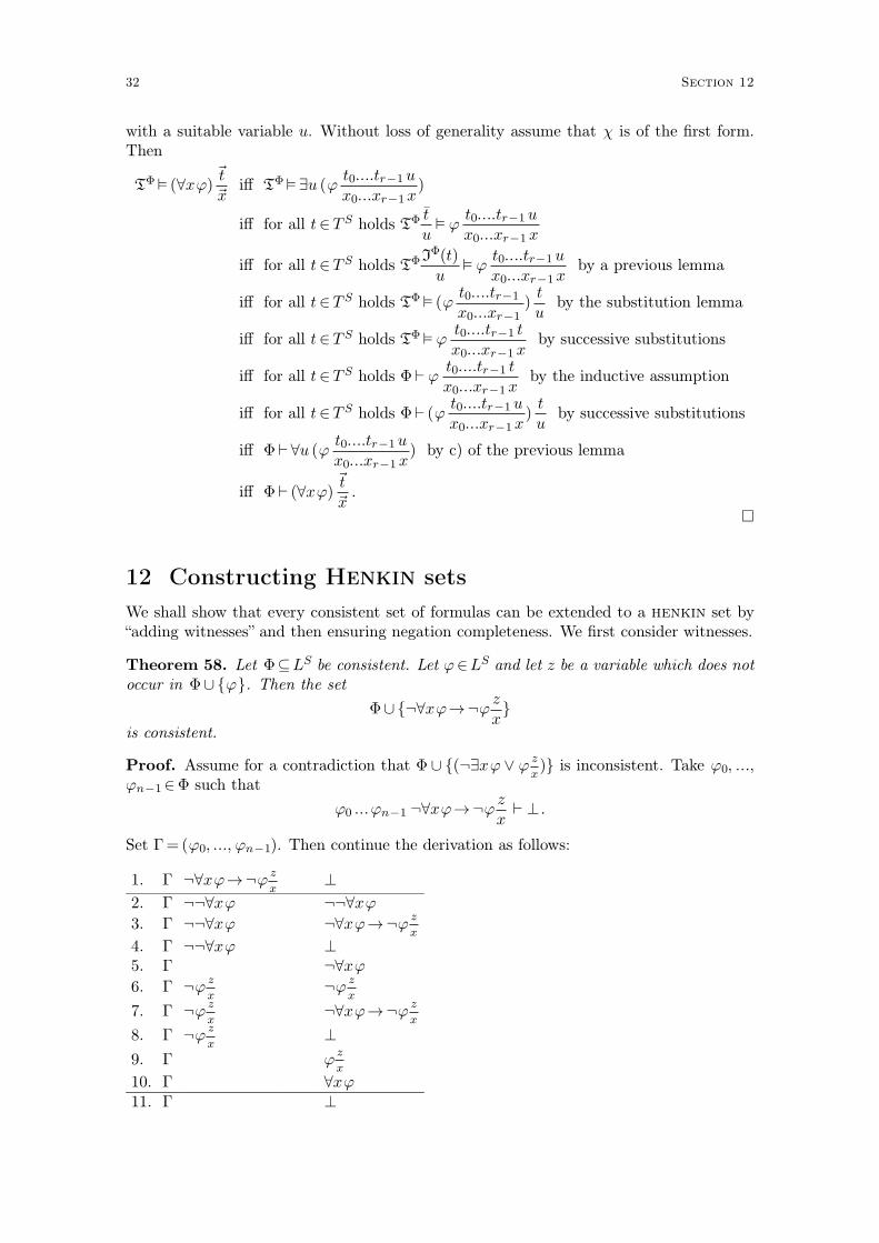
with a suitable variable u. Without loss of generality assume that χ is of the first form.Then
TΦ� (∀xϕ)t~
x~iff TΦ�∃u (ϕ
t0....tr−1 u
x0...xr−1x)
iff for all t∈T S holds TΦ t̄
u� ϕ
t0....tr−1 u
x0...xr−1 x
iff for all t∈T S holds TΦIΦ(t)u
� ϕt0....tr−1 u
x0...xr−1xby a previous lemma
iff for all t∈T S holds TΦ� (ϕt0....tr−1
x0...xr−1)t
uby the substitution lemma
iff for all t∈T S holds TΦ� ϕt0....tr−1 t
x0...xr−1 xby successive substitutions
iff for all t∈T S holds Φ⊢ ϕt0....tr−1 t
x0...xr−1 xby the inductive assumption
iff for all t∈T S holds Φ⊢ (ϕt0....tr−1 u
x0...xr−1x)t
uby successive substitutions
iff Φ⊢∀u (ϕt0....tr−1u
x0...xr−1 x) by c) of the previous lemma
iff Φ⊢ (∀xϕ)t~
x~.
�
12 Constructing Henkin sets
We shall show that every consistent set of formulas can be extended to a henkin set by“adding witnesses” and then ensuring negation completeness. We first consider witnesses.
Theorem 58. Let Φ⊆LS be consistent. Let ϕ∈LS and let z be a variable which does notoccur in Φ∪ {ϕ}. Then the set
Φ∪ {¬∀xϕ→¬ϕz
x}
is consistent.
Proof. Assume for a contradiction that Φ ∪ {(¬∃xϕ ∨ ϕz
x)} is inconsistent. Take ϕ0, ...,
ϕn−1∈Φ such that
ϕ0 ...ϕn−1 ¬∀xϕ→¬ϕz
x⊢ ⊥ .
Set Γ=(ϕ0, ..., ϕn−1). Then continue the derivation as follows:
1. Γ ¬∀xϕ→¬ϕz
x⊥
2. Γ ¬¬∀xϕ ¬¬∀xϕ
3. Γ ¬¬∀xϕ ¬∀xϕ→¬ϕz
x
4. Γ ¬¬∀xϕ ⊥5. Γ ¬∀xϕ
6. Γ ¬ϕz
x¬ϕ
z
x
7. Γ ¬ϕz
x¬∀xϕ→¬ϕ
z
x
8. Γ ¬ϕz
x⊥
9. Γ ϕz
x
10. Γ ∀xϕ11. Γ ⊥
32 Section 12
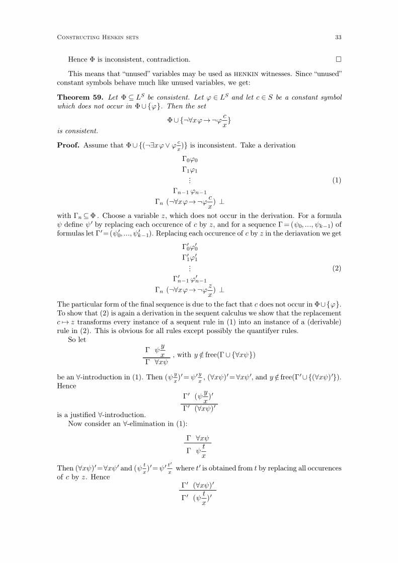
Hence Φ is inconsistent, contradiction. �
This means that “unused” variables may be used as henkin witnesses. Since “unused”constant symbols behave much like unused variables, we get:
Theorem 59. Let Φ ⊆ LS be consistent. Let ϕ ∈ LS and let c ∈ S be a constant symbolwhich does not occur in Φ∪ {ϕ}. Then the set
Φ∪ {¬∀xϕ→¬ϕc
x}
is consistent.
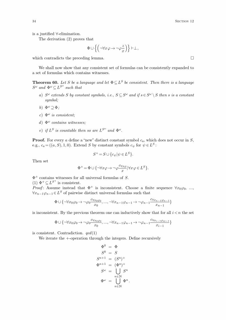
Proof. Assume that Φ∪ {(¬∃xϕ∨ ϕc
x)} is inconsistent. Take a derivation
Γ0ϕ0
Γ1ϕ1
··· (1)
Γn−1 ϕn−1
Γn (¬∀xϕ→¬ϕc
x) ⊥
with Γn ⊆Φ . Choose a variable z, which does not occur in the derivation. For a formulaψ define ψ ′ by replacing each occurence of c by z, and for a sequence Γ=(ψ0, ..., ψk−1) offormulas let Γ′=(ψ0
′ , ...,ψk−1′ ). Replacing each occurence of c by z in the deriavation we get
Γ0′ϕ0
′
Γ1′ϕ1
′
··· (2)
Γn−1′ ϕn−1
′
Γn (¬∀xϕ→¬ϕz
x) ⊥
The particular form of the final sequence is due to the fact that c does not occur in Φ∪{ϕ}.To show that (2) is again a derivation in the sequent calculus we show that the replacementc 7→ z transforms every instance of a sequent rule in (1) into an instance of a (derivable)rule in (2). This is obvious for all rules except possibly the quantifyer rules.
So let
Γ ψy
xΓ ∀xψ
, with y ∈/ free(Γ∪ {∀xψ})
be an ∀-introduction in (1). Then (ψy
x)′= ψ ′ y
x, (∀xψ)′=∀xψ ′, and y∈/ free(Γ′∪{(∀xψ)′}).
Hence
Γ′ (ψy
x)′
Γ′ (∀xψ)′is a justified ∀-introduction.
Now consider an ∀-elimination in (1):
Γ ∀xψ
Γ ψt
x
Then (∀xψ)′=∀xψ ′ and (ψt
x)′=ψ ′ t
′
xwhere t′ is obtained from t by replacing all occurences
of c by z. HenceΓ′ (∀xψ)′
Γ′ (ψt
x)′
Constructing Henkin sets 33
is a justified ∀-elimination.
The derivation (2) proves that
Φ∪n�
¬∀xϕ→¬ϕz
x
�o
⊢⊥ ,
which contradicts the preceding lemma. �
We shall now show that any consistent set of formulas can be consistently expanded toa set of formulas which contains witnesses.
Theorem 60. Let S be a language and let Φ⊆LS be consistent. Then there is a languageSω and Φω ⊆LSω
such that
a) Sω extends S by constant symbols, i.e., S ⊆Sω and if s∈Sω \S then s is a constantsymbol;
b) Φω ⊇Φ;
c) Φω is consistent;
d) Φω contains witnesses;
e) if LS is countable then so are LSωand Φω.
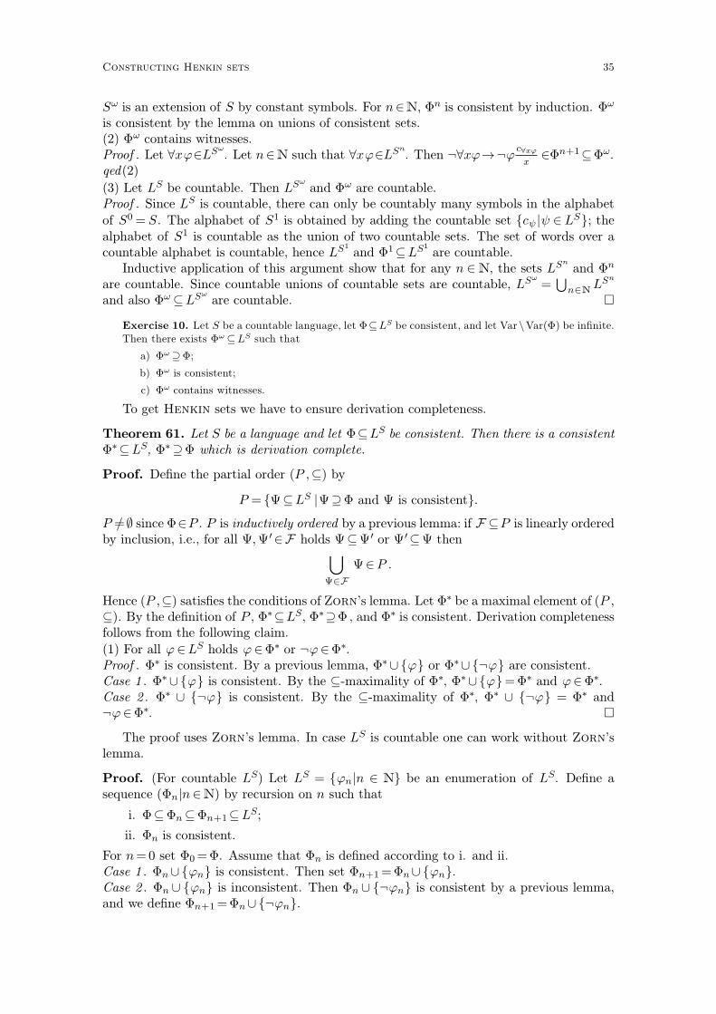
Proof. For every a define a “new” distinct constant symbol ca, which does not occur in S,e.g., ca= ((a, S), 1, 0). Extend S by constant symbols cψ for ψ ∈LS :
S+=S ∪ {cψ |ψ ∈LS}.
Then set
Φ+=Φ∪ {¬∀xϕ→¬ϕc∀xϕx
|∀xϕ∈LS}.
Φ+ contains witnesses for all universal formulas of S.(1) Φ+⊆LS+
is consistent.Proof : Assume instead that Φ+ is inconsistent. Choose a finite sequence ∀x0ϕ0, ...,
∀xn−1ϕn−1∈LS of pairwise distinct universal formulas such that
Φ∪ {¬∀x0ϕ0→¬ϕ0c∀x0ϕ0
x0, ...,¬∀xn−1ϕn−1→¬ϕn−1
c∀xn−1ϕn−1
xn−1}
is inconsistent. By the previous theorem one can inductively show that for all i<n the set
Φ∪ {¬∀x0ϕ0→¬ϕ0c∀x0ϕ0
x0, ...,¬∀xn−1ϕn−1→¬ϕn−1
c∀xi−1ϕni−1
xi−1}
is consistent. Contradiction. qed(1)
We iterate the +-operation through the integers. Define recursively
Φ0 = Φ
S0 = S
Sn+1 = (Sn)+
Φn+1 = (Φn)+
Sω =[
n∈N
Sn
Φω =[
n∈N
Φn .
34 Section 12
Sω is an extension of S by constant symbols. For n∈N, Φn is consistent by induction. Φω
is consistent by the lemma on unions of consistent sets.(2) Φω contains witnesses.Proof . Let ∀xϕ∈LSω
. Let n∈N such that ∀xϕ∈LSn. Then ¬∀xϕ→¬ϕ
c∀xϕ
x∈Φn+1⊆Φω.
qed(2)
(3) Let LS be countable. Then LSωand Φω are countable.
Proof . Since LS is countable, there can only be countably many symbols in the alphabet
of S0 = S. The alphabet of S1 is obtained by adding the countable set {cψ |ψ ∈ LS}; thealphabet of S1 is countable as the union of two countable sets. The set of words over acountable alphabet is countable, hence LS1
and Φ1⊆LS1
are countable.Inductive application of this argument show that for any n ∈N, the sets LSn
and Φn
are countable. Since countable unions of countable sets are countable, LSω=S
n∈NLSn
and also Φω ⊆LSωare countable. �
Exercise 10. Let S be a countable language, let Φ⊆LS be consistent, and let Var\Var(Φ) be infinite.Then there exists Φω ⊆LS such that
a) Φω ⊇Φ;
b) Φω is consistent;
c) Φω contains witnesses.
To get Henkin sets we have to ensure derivation completeness.
Theorem 61. Let S be a language and let Φ⊆LS be consistent. Then there is a consistentΦ∗⊆LS, Φ∗⊇Φ which is derivation complete.
Proof. Define the partial order (P ,⊆) by
P = {Ψ⊆LS |Ψ⊇Φ and Ψ is consistent}.
P =/ ∅ since Φ∈P . P is inductively ordered by a previous lemma: if F ⊆P is linearly orderedby inclusion, i.e., for all Ψ,Ψ′∈F holds Ψ⊆Ψ′ or Ψ′⊆Ψ then
[
Ψ∈F
Ψ∈P .
Hence (P ,⊆) satisfies the conditions of Zorn’s lemma. Let Φ∗ be a maximal element of (P ,
⊆). By the definition of P , Φ∗⊆LS, Φ∗⊇Φ , and Φ∗ is consistent. Derivation completenessfollows from the following claim.
(1) For all ϕ∈LS holds ϕ∈Φ∗ or ¬ϕ∈Φ∗.Proof . Φ∗ is consistent. By a previous lemma, Φ∗∪ {ϕ} or Φ∗∪ {¬ϕ} are consistent.Case 1 . Φ∗∪ {ϕ} is consistent. By the ⊆-maximality of Φ∗, Φ∗∪ {ϕ}=Φ∗ and ϕ∈Φ∗.Case 2 . Φ∗ ∪ {¬ϕ} is consistent. By the ⊆-maximality of Φ∗, Φ∗ ∪ {¬ϕ} = Φ∗ and¬ϕ∈Φ∗. �
The proof uses Zorn’s lemma. In case LS is countable one can work without Zorn’slemma.
Proof. (For countable LS) Let LS = {ϕn|n ∈ N} be an enumeration of LS. Define asequence (Φn|n∈N) by recursion on n such that
i. Φ⊆Φn⊆Φn+1⊆LS;
ii. Φn is consistent.
For n=0 set Φ0=Φ. Assume that Φn is defined according to i. and ii.Case 1 . Φn∪ {ϕn} is consistent. Then set Φn+1=Φn∪ {ϕn}.Case 2 . Φn ∪ {ϕn} is inconsistent. Then Φn ∪ {¬ϕn} is consistent by a previous lemma,and we define Φn+1=Φn∪ {¬ϕn}.
Constructing Henkin sets 35
Let
Φ∗=[
n∈N
Φn .
Then Φ∗ is a consistent superset of Φ. By construction, ϕ∈Φ∗ or ¬ϕ∈Φ∗, for all ϕ∈LS.Hence Φ∗ is derivation complete. �
According to Theorem 60 a given consistent set Φ can be extended to Φω ⊆ LSω
containing witnesses. By Theorem 61 Φω can be extended to a derivation complete Φ∗⊆LSω
. Since the latter step does not extend the language, Φ∗ contains witnesses and is thusa henkin set:
Theorem 62. Let S be a language and let Φ⊆LS be consistent. Then there is a languageS∗ and Φ∗⊆LS∗
such that
a) S∗⊇S is an extension of S by constant symbols;
b) Φ∗⊇Φ is a Henkin set;
c) if LS is countable then so are LS∗
and Φ∗.
13 The completeness theorem
The development of mathematics
towards greater precision has led,
as is well known, to the formaliz-
ation of large tracts of it, so that
one can prove any theorem using
nothing but a few mechanical rules.
Kurt Gödel, 1941
We can now combine our technical preparations to show the fundamental theoremsof first-order logic. Combining Theorems 62 and 57, we obtain a general and a countablemodel existence theorem:
Theorem 63. (Henkin model existence theorem) Let Φ⊆ LS. Then Φ is consistent iffΦ is satisfiable.
By Lemma 51, Theorem 63 the model existence theorems imply the main theorem.
Theorem 64. (Gödel completeness theorem) The sequent calculus is complete, i.e.,�=⊢.
TheGödel completeness theorem is the fundamental theorem of mathematical logic. Itconnects syntax and semantics of formal languages in an optimal way. Before we continuethe mathematical study of its consequences we make some general remarks about the widerimpact of the theorem:
− The completeness theorem gives an ultimate correctness criterion for mathematicalproofs. A proof is correct if it can (in principle) be reformulated as a formal deriv-ation. Although mathematicians prefer semi-formal or informal arguments, thiscriterion could be applied in case of doubt.
36 Section 13
− Checking the correctness of a formal proof in the above sequent calculus is asyntactic task that can be carried out by computer. We shall later consider aprototypical proof checker Naproche which uses a formal language which is a subsetof natural english.
− By systematically running through all possible formal proofs, automatic theoremproving is in principle possible. In this generality, however, algorithms immediatelyrun into very high algorithmic complexities and become practically infeasable.
− Practical automatic theorem proving has become possible in restricted situations,either by looking at particular kinds of axioms and associated intended domains, orby restricting the syntactical complexity of axioms and theorems.
− Automatic theorem proving is an important component of artificial intelligence(AI) where a system has to obtain logical consequences from conditions formulatedin first-order logic. Although there are many difficulties with artificial intelligencethis approach is still being followed with some success.
− Another special case of automatic theorem proving is given by logic programmingwhere programs consist of logical statements of some restricted complexity and arun of a program is a systematic search for a solution of the given statements. Theoriginal and most prominent logic programming language is Prolog which is stillwidely used in linguistics and AI.
− There are other areas which can be described formally and where syntax/semanticsconstellations similar to first-order logic may occur. In the theory of algorithmsthere is the syntax of programming languages versus the (mathematical) meaningof a program. Since programs crucially involve time alternative logics with timehave to be introduced. Now in all such generalizations, the Gödel completenesstheorem serves as a pattern onto which to model the syntax/semantics relation.
− The success of the formal method in mathematics makes mathematics a leadingformal science. Several other sciences also strive to present and justify results form-ally, like computer science and parts of philosophy.
− The completeness theorem must not be confused with the famous Gödel incom-pleteness theorems: they say that certain axiom systems like Peano arithmetic areincomplete in the sense that they do not imply some formulas which hold in thestandard model of the axiom system.
14 The compactness theorem
The equality of � and ⊢ and the compactness theorem 43 for ⊢ imply
Theorem 65. (Compactness theorem) Let Φ⊆LS and ϕ∈Φ . Then
a) Φ� ϕ iff there is a finite subset Φ0⊆Φ such that Φ0� ϕ .
b) Φ is satisfiable iff every finite subset Φ0⊆Φ is satisfiable.
This theorem is often to construct (unusual) models of first-order theories. It is thebasis of a field of logic called Model Theory .
We present a number theoretic application of the compactness theorem. The languageof arithmetic can be naturally interpreted in the structure N=(N,+, ·,0,1). This structureobviously satisfies the following axioms:
The compactness theorem 37
Definition 66. The axiom system PA ⊆ LSAR of peano arithmetic consists of the fol-lowing sentences
− ∀x x+1=/ 0
− ∀x∀y x+1= y+1→x= y
− ∀x x+0= x
− ∀x∀y x+(y+1)= (x+ y)+ 1
− ∀x x · 0= 0
− ∀x∀y x · (y+1)=x · y+x
− Schema of induction: for every formula ϕ(x0, ..., xn−1, xn)∈LSAR:
∀x0...∀xn−1(ϕ(x0, ..., xn−1, 0)∧∀xn(ϕ→ ϕ(x0, ..., xn−1, xn+1))→∀xnϕ)
The theory PA is allows to prove a lot of number theoretic properties, e.g., aboutdivisibility and prime numbers. On the other hand the first incompleteness theorem ofGödel shows that there are arithmetic sentences ϕ which are not decided by PA althoughthey are true in the standard model N of PA. Therefore PA is not complete.
If ϕ and ¬ϕ are both not derivable from PA then PA+¬ϕ and PA+ ϕ are consistent.By the model existence theorem, there are models M− and M+ such that M−�PA+¬ϕand M+ � PA+ ϕ. M− and M+ are not isomorphic. So there exist models of PA whichare not isomorphic to the standard model N.
We can also use the compactness theorem to obtain nonstandard models of theories.Define the SAR-terms n̄ for n∈N recursively by
0̄ = 0,
n+1 = (n̄+1).
Define divisibility by the SAR-formula δ(x, y)=∃z x · z≡ y.
Theorem 67. There is a model M�PA which contains an element ∞∈M, ∞=/ 0̄M suchthat M � δ(n̄,∞) for every n∈N \ {0} (we use M � δ(n̄,∞) as an intuitive abbreviationfor M� δ(n̄, v0)[∞]).
So “from the outside”, ∞ is divisible by every positive natural number. This impliesthat M is a nonstandard model with M=∼/ N .
Proof. Consider the theory
Φ=PA∪ {δ(n̄, v0) |n∈N \ {0}}∪ {¬v0≡ 0̄}
(1) Φ is satisfiable.Proof . We use the compactness theorem 65(b). Let Φ0 ⊆ Φ be finite. It suffices to showthat Φ0 is satisfiable. Take a finite number n0∈N such that
Φ0⊆PA∪ {δ(n̄, v0) |n∈N, 16n6n0}.
Let N =n! . Then
N�PA and N� δ(n̄, N) for 16n6n0 .
So NN
v0�Φ0 . qed(1)
By (1), let M′�Φ. Let ∞=M′(v0)∈ |M′|. Let M be the SAR-structure which extendsto the modelM′, i.e.,M=M′↾{∀}∪SAR . ThenM is a structure satisfying the theorem. �
38 Section 14
This indicates that the model class of PA is rather complicated and rich. Indeed thereis a subfield of model theory which studies models of Peano arithmetic.
We define notions which allow to examine the axiomatizability of classes of structures.
Definition 68. Let S be a language and K be a class of S-structures.
a) K ist elementary or finitely axiomatizable if there is an S-sentence ϕ with K =
ModSϕ.
b) K is Δ-elementary or axiomatizable, if there is a set Φ of S-sentences with K =
ModSΦ.
We state simple properties of the Mod-operator:
Theorem 69. Let S be a language.Then
a) For Φ⊆Ψ⊆L0S holds ModSΦ⊇ModSΨ.
b) For Φ,Ψ⊆L0S holds ModS(Φ∪Ψ)=ModSΦ∩ModSΨ.
c) For Φ⊆L0S holds ModSΦ=
T
ϕ∈ΦModSϕ .
d) For ϕ0, ..., ϕn−1∈L0S holds ModS{ϕ0, ..., ϕn−1}=ModS(ϕ0∧ ...∧ ϕn−1).
e) For ϕ∈L0S holds ModS(¬ϕ)=ModS(∅) \ModS(ϕ).
c) explains the denotation “Δ-elementary”, since ModSΦ is the intersection (“Durch-schnitt”) of all single ModSϕ .
Theorem 70. Let S be a language and K,L be classes of S-structures with
L=ModS∅\K .
Then if K and L are axiomatizable, they are finitely axiomatizable.
Proof. Take axiom systems ΦK and ΦL such that K=ModSΦK and L=ModSΦL. Assumethat K is not finitely axiomatizable.(1) Let Φ0⊆ΦK be finite. Then Φ0∪ΦL is satisfiable.Proof : ModSΦ0 ⊇ModSΦK . Since K is not finitely axiomatizable, ModSΦ0 =/ ModSΦK .
Then ModSΦ0∩L=/ ∅. Take a model A∈L, A∈ModSΦ0 . Then A�Φ0∪ΦL . qed(1)(2) ΦK ∪ΦL is satisfiable.Proof : By the compactness theorem 65 it suffices to show that every finite Ψ⊆ ΦK ∪ ΦL
is satsifiable. By (1), (Ψ∩ΦK)∪ΦL is satisfiable. Thus Ψ⊆ (Ψ∩ΦK)∪ΦL is satisfiable.qed(2)
By (2), ModSΦK ∩ModSΦL=/ ∅. But the classes K and L are complements, contradic-tion. Thus K is finitely axiomatizable. �
15 The Löwenheim-Skolem theorems
Definition 71. An S-structure A is finite, infinite, countable, or uncountable, resp., iffthe underlying set |A| is finite, infinite, countable, or uncountable, resp..
If the language S is countable, i.e., finite or countably infinite, and it Φ ⊆ LS is acountable consistent set of formulas then an inspection of the above construction of a termmodel for Φ shows the following theorem.
The Löwenheim-Skolem theorems 39
Theorem 72. (Downward Löwenheim-Skolem theorem) Let Φ ⊆ LS be a countableconsistent set of formulas. Then Φ possesses a model M= (A, β)�Φ, A= (A, ...) with acountable underlying set A.
The word “downward” emphasises the existence of models of “small” cardinality. Weshall soon consider an “upward” Löwenheim-Skolem theorem.
Theorem 73. Assume that Φ ⊆ LS has arbitrarily large finite models. Then Φ has aninfinite model.
Proof. For n∈N define the sentence
ϕ�n= ∃v0, ..., vn−1
^
i<j<n
¬vi≡ vj ,
where the big conjunction is defined by^
i<j<n
ψij=ψ0,1∧ ...∧ ψ0,n−1∧ ψ1,2∧ ...∧ ψ1,n−1∧ ...∧ ψn−1,n−1 .
For any model M
M� ϕ�n iff A has at least n elements.
Now set
Φ′=Φ∪ {ϕ�n |n∈N}.
(1) Φ′ has a model.Proof . By the compactness theorem 65b it suffices to show that every finite Φ0⊆Φ has amodel. Let Φ0⊆Φ be finite. Take n0∈N such that
Φ0⊆Φ∪ {ϕ�n |n6n0}.
By assumption Φ has a model with at least n0 elements. Thus Φ∪ {ϕ�n |n6n0} and Φ0
have a model. qed(1)Let M�Φ′. Then M is an infinite model of Φ. �
Theorem 74. (Upward Löwenheim-Skolem theorem) Let Φ⊆ LS have an infinite S-model and let X be an arbitrary set. Then Φ has a model into which X can be embeddedinjectively.
Proof. Let M be an infinite model of Φ. Choose a sequence (cx |x ∈ X) of pairwisedistinct constant symbols which do not occur in S, e.g., setting cx = ((x, S), 1, 0). LetS ′=S ∪ {cx |x∈X} be the extension of S by the new constant symbols. Set
Φ′=Φ∪ {¬cx≡ cy |x, y ∈X,x=/ y}.
(1) Φ′ has a model.Proof . It suffices to show that every finite Φ0⊆Φ′ has a model. Let Φ0⊆Φ′ be finite. Takea finite set X0⊆X such that
Φ0⊆Φ∪ {¬cx≡ cy |x, y ∈X0, x=/ y}.
Since |M| is infinite we can choose an injective sequence (ax|x ∈ X0) of elements of |M|such that x=/ y implies ax=/ ay . For x ∈X \X0 choose ax ∈ |M| arbitrarily. Then in theextended model
M′=M∪ {(cx, ax)|x∈X}�Φ∪ {¬cx≡ cy |x, y ∈X0, x=/ y}⊇Φ0 .
qed(1)
40 Section 15
By (1), choose a model M′�Φ′. Then the map
i:X→ |M′|, x 7→M′(cx)
is injective. The reduct M′′=M′ ↾ {∀}∪S is as required. �
Theorem 75. Let S be a language.
a) The class of all finite S-structures is not axiomatizable.
b) The class of all infinite S-structures is axiomatizable but not finitely axiomatizable.
Proof. a) is immediate by Theorem 73.b) The class of infinite S-structures is axiomatized by
Φ= {ϕ�n |n∈N}.
If that class were finitely axiomatizable then the complementary class of finite S-structureswould also be (finitely) axiomatizable, contradicting a). �
16 Normal forms
There are many motivations to transform formulas into equivalent normal forms . Themotivation here will be that normal forms are important for automated theorem provingand for logic programming .
We are particularly interested in transforming formulas ψ into formulas ψ ′ such that ψis consistent iff ψ ′ is consistent. This relates to provability as follows: Φ⊢ ϕ iff Φ∪{¬ϕ} isnot satisfiable/inconsistent. So a check for provability can be based on inconsistency checks.
Work in some fixed language S.
Definition 76.
a) An S-formula is a literal if it is atomic or the negation of an atomic formula.
b) Define the dual of the literal L as
L̄=
�
¬L, if L is an atomic formula;K, if L is of the form ¬K.
c) A formula ϕ is in disjunctive normal form if it is of the form
ϕ=_
i<m
(^
j<ni
Lij)
where each Lij is a literal.
d) A formula ϕ is in conjunctive normal form if it is of the form
ϕ=^
i<m
(_
j<ni
Lij)
where each Lij is a literal. Sometimes a disjunctive normal form is also written inset notion as
ϕ= {{L00, ..., L0n0−1}, ..., {Lm−1,0, ..., Lm−1,nm−1}}.
Theorem 77. Let ϕ be a formula without quantifiers. Then ϕ is equivalent to some ϕ′ indisjunctive normal form and to some ϕ′′ in conjunctive normal form.
Normal forms 41
Proof. By induction on the complexity of ϕ. Clear for ϕ atomic. The ¬ step follows fromthe de Morgan laws:
¬_
i<m
(^
j<ni
Lij) ↔^
i<m
¬(^
j<ni
Lij)
↔^
i<m
(_
j<ni
¬Lij).
The ∧-step is clear for conjunctive normal forms. For disjunctive normal forms the asso-ciativity rules yield
_
i<m
(^
j<ni
Lij)∧_
i<m′
(^
j<ni′
Lij′ ) ↔
_
i<m,i′<m′
(^
j<ni
Lij ∧^
j<ni′
Lij′ )
which is also in conjunctive normal form. �
Definition 78. A formula ϕ is in prenex normal form if it is of the form
ϕ=Q0 x0 Q1 x1...Qm−1 xm−1 ψ
where each Qi is either the quantifier ∀ or ∃ and ψ is quantifier-free. Then the quantifierstring Q0 x0 Q1 x1...Qm−1 xm−1 is called the prefix of ϕ and the formula ψ is the matrixof ϕ.
Theorem 79. Let ϕ be a formula. Then ϕ is equivalent to a formula ϕ′ in prenex normalform.
Proof. By induction on the complexity of ϕ. Clear for atomic formulas. If
ϕ↔Q0x0 Q1 x1...Qm−1xm−1 ψ
with quantifier-free ψ then by the de Morgan laws for quantifiers
¬ϕ↔ Q̄0x0 Q̄1 x1... Q̄m−1xm−1¬ψ
where the dual quantifier Q̄ is defined by ∃̄=∀ and ∀̄=∃ .For the ∧-operation consider another formula
ϕ′↔Q0′ x0
′ Q1′ x1
′ ...Qm′−1′ xm′−1
′ ψ ′
with quantifier-free ψ ′. We may assume that the bound variables of of the prenex normalforms are disjoint. Then
ϕ∧ ϕ′↔Q0x0 Q1 x1...Qm−1xm−1Q0′ x0
′ Q1′ x1
′ ...Qm′−1′ xm ′−1
′ (ψ ∧ ψ ′).
(semantic argument). �
Definition 80. A formula ϕ is universal if it is of the form
ϕ= ∀x0∀x1...∀xm−1 ψ
where ψ is quantifier-free. A formula ϕ is existential if it is of the form
ϕ= ∃x0∃x1...∃xm−1 ψ
where ψ is quantifier-free.
We show a quasi-equivalence with respect to universal (and existential) formulas whichis not a logical equivalence but concerns the consistency or satisfiability of formulas.
42 Section 16

Theorem 81. Let ϕ be an S-formula. Then there is a canonical extension S∗ of thelanguage S and a canonical universal ϕ∗∈LS∗
such that
ϕ is consistent iff ϕ∗ is consistent.
The formula ϕ∗ is called the Skolem normal form of ϕ.
Proof. By a previous theorem we may assume that ϕ is in prenex normal form. We provethe theorem by induction on the number of existential quantifiers in ϕ. If ϕ does notcontain an existential quantifier we are done. Otherwise let
ϕ=∀x1...∀xm∃yψ
where m < ω may also be 0. Introduce a new m-ary function symbol f (or a constantsymbol in case m=0) and let
ϕ′=∀x1...∀xmψfx1...xm
y.
By induction it suffices to show that ϕ is consistent iff ϕ′ is consistent.(1) ϕ′→ ϕ.Proof . Assume ϕ′. Consider x1, ..., xm . Then ψ
fx1...xm
y. Then ∃yψ. Thus ∀x1...∀xm∃yψ.
qed(1)(2) If ϕ′ is consistent then ϕ is consistent.Proof . If ϕ→⊥ then by (1) ϕ′→⊥ . qed(2)(3) If ϕ is consistent then ϕ′ is consistent.Proof . Let ϕ be consistent and let M=(M, ...)� ϕ . Then
∀a1∈M ...∀am∈M ∃b∈MMa~ b
x~ y�ψ .
Using the axiom of choice there is a function h:Mm→M such that
∀a1∈M ...∀am∈MMa~ h(a1, ..., am)
x~ y�ψ .
Expand the structure M to M′=M∪ {(f , h)} where the symbol f is interpreted by the
function h. Then h(a1, ..., am)=M′a~
x~(fx1...xm) and
∀a1∈M ...∀am∈MM′a~ M′a~
x~(fx1...xm)
x~ y=M′a~
x~
M′a~
x~(fx1...xm)
y� ψ .
By the substitution theorem this is equivalent to
∀a1∈M ...∀am∈M M′a~
x~� ψ
fx1...xm
y.
Hence
M′� ∀x1...∀xmψfx1...xm
y=ϕ′.
Thus ϕ′ is consistent. �
17 Herbrand’s theorem
By the previous chapter we can reduce the question whether a given finite set of formulasis inconsistent to the question whether some universal formula is inconsistent. By thefollowing theorem this can be answered rather concretely.
Herbrand’s theorem 43
Theorem 82. Let S be a language which contains at least one constant symbol. Let
ϕ= ∀x0∀x1...∀xm−1 ψ
be a universal S-sentence with quantifier-free matrix ψ . Then ϕ is inconsistent if there arevariable-free S-terms (“constant terms”)
t00, ..., tm−1
0 , ..., t0N−1, ..., tm−1
N−1
such that
ϕ′=^
i<N
ψt0i , ..., tm−1
i
x0, ..., xm−1=ψ
t00, ..., tm−1
0
x0, ..., xm−1∧ ...∧ ψ
t0N−1, ..., tm−1
N−1
x0, ..., xm−1
is inconsistent.
Proof. All sentences ϕ′, for various choices of constant terms, are logical consequences ofϕ. So ϕ is consistent, all ϕ′ are consistent.
Conversely assume that all ϕ′ are consistent. Then by the compactness theorem
Φ= {ψt0, ..., tm−1
x0, ..., xm−1|t0, ..., tm−1 are constant S-terms}
is consistent. Let M= (M, ...)�Φ. Let
H = {M(t) |t is a constant S-term}.
Then H =/ ∅ since S contains a constant symbol. By definition, H is closed under thefunctions of M . So we let H=(H, ...)⊆M be the substructure of M with domain H.(1) H � ϕ .Proof . Let M(t0), ..., M(tm−1) ∈ H where t0, ..., tm−1 are constant S-terms. Then
ψt0, ..., tm−1
x0, ..., xm−1∈Φ, M� ψ
t0, ..., tm−1
x0, ..., xm−1, and by the substitution theorem
MM(t0), ...,M(tm−1)
x0, ..., xm−1� ψ .
Since ψ is quantifier-free this transfers to H :
HM(t0), ...,M(tm−1)
x0, ..., xm−1� ψ .
Thus
H � ∀x0 ∀x1...∀xm−1 ψ= ϕ .
qed(1)Thus ϕ is consistent. �
In case that the formula ψ does not contain the equality sign ≡ checking for inconsist-ency of
ϕ′=^
i<N
ψt0i , ..., tm−1
i
x0, ..., xm−1=ψ
t00, ..., tm−1
0
x0, ..., xm−1∧ ...∧ ψ
t0N−1, ..., tm−1
N−1
x0, ..., xm−1
is in principle a straightforward finitary problem. ϕ′ contains finitely many constant S-terms. ϕ′ is consistent iff the relation symbols can be interpreted on appropriate tuplesof the occuring S-terms to make ϕ′ true. There are finitely many possibilities for theassignments of truth values of relations. This leads to the following (theoretical) algorithmfor automatic proving for formulas without ≡:
Let Ω⊆LS be finite and χ∈LS. To check whether Ω⊢ χ:
1. Form Φ=Ω∪{¬χ} and let ϕ=∀(V
Φ) be the universal closure ofV
Φ . Then Ω⊢ χ
iff Φ=Ω∪ {¬χ} is inconsistent iff (V
Φ)⊢⊥ iff ∀(V
Φ)⊢⊥ .
44 Section 17
2. Transform ϕ into universal form ϕ∀= ∀x0 ∀x1...∀xm−1 ψ (Skolemization).
3. (Systematically) search for constant S-terms
t00, ..., tm−1
0 , ..., t0N−1, ..., tm−1
N−1
such that
ϕ′=^
i<N
ψt0i , ..., tm−1
i
x0, ..., xm−1=ψ
t00, ..., tm−1
0
x0, ..., xm−1∧ ...∧ ψ
t0N−1, ..., tm−1
N−1
x0, ..., xm−1
is inconsistent.
4. If an inconsistent ϕ′ is found, output “yes”, otherwise carry on.
Obviously, if “yes” is output then Ω⊢ χ . This is the correctness of the algorithm. On theother hand, Herbrand’s theorem ensures that if Ω ⊢ χ then an appropriate ϕ′ will befound, and “yes” will be output, i.e., the algorithm is complete.
Example 83. We demonstrate the procedure with a small example. Let
χ=∃x∀y(D(x)→D(y))
be the well-known drinker’s paradox : there is somebody called x such that everybodydrinks provided x drinks. To prove χ we follow the above steps.
1. χ is valid iff ¬χ is inconsistent. ¬χ is equivalent to ∀x∃y(D(x)∧¬D(y)).
2. The Skolemization of that formula is ∀x(D(x)∧¬D(fy(x))).
3. Ground terms without free variables can be formed from a new constant symbol cand the unary function symbol fy : c, fy(c), fy(fy(c)), ... . We form the correspondingground instances of the kernel D(x)∧¬D(fy(x)):
D(c)∧¬D(fy(c)), D(fy(c))∧¬D(fy(fy(c))), D(fy(fy(c)))∧¬D(fy(fy(fy(c)))), ...
This leads to a sequence of conjunctions of ground instances:
− D(c) ∧ ¬D(fy(c)) is consistent since the conjunction does not contain dualliterals;
− D(c) ∧ ¬D(fy(c)) ∧ D(fy(c)) ∧ ¬D(fy(fy(c))) is inconsistent since the
conjunction contains the dual literals ¬D(fy(c)) and D(fy(c)).
This concludes the proof of the drinker’s paradox via Herbrand’s theorem.
18 Simple automatic theorem proving
The syntax of first-order logic works with finite strings of symbols and is amenableto computer implementation. The Handbook of Practical Logic and Automated Reas-oning by John Harrison, Cambridge University Press 2009, contains working programswhich define basic notions of first-order logic including the above proof method basedon Herbrand’s theorem. The programs are written in the functional programming lan-guage OCaml. OCaml programs consist of commands which are similar to mathematicaldefinitions of constants and functions. The OCaml programs of the Handbook are avail-able via the website http://www.cl.cam.ac.uk/~jrh13/atp/index.html.
Harrison defines the type (or class or set) of terms recursively as:
Simple automatic theorem proving 45
type term = Var of string
| Fn of string * term list;;
(Relational) atomic formulas are given by
type fol = R of string * term list;;
The atomic formula D(x) of the drinker’s formula is thus
R("D",[Var "x"])
Formulas are defined generally over any type (’a) of atomic formulas
type (’a)formula = False
| True
| Atom of ’a
| Not of (’a)formula
| And of (’a)formula * (’a)formula
| Or of (’a)formula * (’a)formula
| Imp of (’a)formula * (’a)formula
| Iff of (’a)formula * (’a)formula
| Forall of string * (’a)formula
| Exists of string * (’a)formula;;
First-order formulas in particular are those of type fol formula where fol has beendefined above. The drinker’s paradox is expressed in this language as
Exists("x",Forall("y",Imp(Atom(R("D",[Var "x"])),Atom(R("D",[Var "y"])))))
To improve readability, a pretty printer for the type fol formula is defined and automat-ically invoked. Entering the drinker’s formula into an interactive OCaml terminal resultsin the following dialogue:
# Exists("x",Forall("y",Imp(Atom(R("D",[Var "x"])),Atom(R("D",[Var
"y"])))));;
- : fol formula = <<exists x. forall y. D(x) ==> D(y)>>
The result of the query is output in the bottom line: the input is recognized by typeinference as a first-order formula; the value of the input is then reprinted readably by thepretty printer; the << >> quotes signal the “pretty format”. Formulas can also be input inthe pretty format. We define the drinker’s formula χ by:
# let chi = <<exists x. forall y. D(x) ==> D(y)>>;;
val chi : fol formula = <<exists x. forall y. D(x) ==> D(y)>>
The definition of χ is acknowledged by stating that the value of chi is now the drinker’sformula. In the Herbrand procedure, a formula to be proved is generalized, negated andskolemized. These operations are implemented by certain functions defined by Harrison:
46 Section 18
# generalize chi;;
- : fol formula = <<exists x. forall y. D(x) ==> D(y)>>
# Not (generalize chi);;
- : fol formula = <<exists x. forall y. D(x) ==> D(y)>>
# skolemize (Not (generalize chi));;
- : fol formula = <<D(x) /\ ~D(f_y(x))>>
The Paul Gilmore in the 1950’s was one of the first to implement the Herbrand pro-cedure. Gilmore’s algorithm is implemented in the Handbook :
let gilmore_loop =
let mfn djs0 ifn djs =
filter (non trivial) (distrib (image (image ifn) djs0) djs) in
herbloop mfn (fun djs -> djs <> []);;
let gilmore fm =
let sfm = skolemize(Not(generalize fm)) in
let fvs = fv sfm and consts,funcs = herbfuns sfm in
let cntms = image (fun (c,_) -> Fn(c,[])) consts in
length(gilmore_loop (simpdnf sfm) cntms funcs fvs 0 [[]] [] []);;
After generalizing, negating and skolemizing, constants and function symbols are extractedand used to generate ground terms and ground instances of the matrix of the skolemizedformula in some recursive loop. Then an inconsistency is searched by transforming for-mulas into disjunctive normal form and checking for inconsistent literals. Details of thesealgorithms are explained in the the Handbook . We prove the drinker’s paradox by applyingthe function gilmore to the formula chi:
# gilmore chi;;
0 ground instances tried; 1 items in list
0 ground instances tried; 1 items in list
1 ground instances tried; 1 items in list
1 ground instances tried; 1 items in list
- : int = 2
The output gives some information about the progress of the search procedure, in particularthat it finishes with “search length” 2, and thus that the claim has been proved.
The Gilmore procedure is able to prove some simple, yet interesting results. The Rus-
sell paradox says that there is no x such that x= {y |y ∈/ y}, i.e., such that ∀y(y ∈ x↔y ∈/ y). We can define and prove the Russell paradox:
# let russell = <<~(exists x. forall y. Elem(y,x) <=> ~Elem(y,y))>>;;
val russell : fol formula =
<<~(exists x. forall y. Elem(y,x) <=> ~Elem(y,y))>>
# gilmore russell;;
0 ground instances tried; 1 items in list
0 ground instances tried; 1 items in list
- : int = 1
Exercise 11. Apply the Herbrand procedure to the Russell paradox “by hand”.
Simple automatic theorem proving 47
19 Resolution
The Gilmore procedure is theoretically complete: a formula is provable iff the procedureterminates. Termination can however take very long so that a proof will not be found inpractice. Also there is an enormous amount of data to be stored which may cause theprogram to crash. E.g., the disjunctive normal forms in the gilmore program which cansimply be checked for inconsistency seem to double in length with each iteration of thealgorithm. Practical automatic theorem proving requires more efficient algorithms in orderto narrow down the search space for inconsistencies and to keep data sizes small.
We shall now present another method based on conjunctive normal forms. We assumethat the quantifier-free formula ψ is a conjunction of clauses ψ= c0∧ c1∧ ...∧ cl−1. Then∀x0 ∀x1...∀xm−1 ψ is inconsistent iff the set
{cit0, ..., tm−1
x0, ..., xm−1|t0, ..., tm−1 are constant S-terms}
is inconsistent.
The method of resolution gives an efficient method for showing the inconsistency of setsof clauses. Let us assume until further notice, that the formulas considered do not containthe symbol ≡.
Definition 84. Let c+= {K0, ...,Kk−1} and c−= {L0, ..., Ll−1} be clauses with literals Ki
and Lj . Note that {K0, ...,Kk−1} stands for the disjunction K0∨ ...∨Kk−1 . Assume thatK0 and L0 are dual, i.e., L0=K0 . Then the disjunction
{K1, ...,Kk−1}∪ {L1, ..., Ll−1}
is a resolution of c+ and c−.
Resolution is related to the application of modus ponens: ϕ→ ψ and ϕ correspond tothe clauses {¬ϕ, ψ} and {ϕ}. {ψ} is a resolution of {¬ϕ, ψ} and {ϕ}.
Theorem 85. Let C be a set of clauses and let c be a resolution of two clauses c+, c−∈C.Then if C ∪ {c} is inconsistent then C is inconsistent.
Proof. Let c+= {K0, ...,Kk−1}, c−= {¬K0, L1..., Ll−1}, and c= {K1, ...,Kk−1}∪ {L1, ...,
Ll−1}. Assume that M�C is a model of C.Case 1 . M�K0 . Then M� c−, M� {L1..., Ll−1}, and
M� {K1, ..., Kk−1}∪ {L1, ..., Ll−1}= c.
Case 2 . M�¬K0 . Then M� c+, M� {K1...,Kk−1}, and
M� {K1, ..., Kk−1}∪ {L1, ..., Ll−1}= c.
Thus M�C ∪ {c}. �
Theorem 86. Let C be a set of clauses closed under resolution. Then C is inconsistentiff ∅∈C. Note that the empty clause {} is logically equivalent to ⊥ .
Proof. If ∅∈C then C is clearly inconsistent.
Assume that the converse implication is false. Consider an set C of clauses such that
(∗) C is inconsistent and closed under resolution, but ∅∈/ C .
48 Section 19
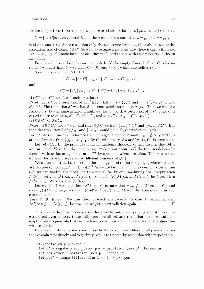
By the compactness theorem there is a finite set of atomic formulas {ϕ0, ...,ϕn−1} such that
C ′= {c∈C |for every literal L in c there exists i < n such that L= ϕi or L=¬ϕi},
is also inconsistent. Since resolution only deletes atomic formulas, C ′ is also closed underresolution, and of course ∅∈/C ′. So we may assume right away that there is only a finite set{ϕ0, ..., ϕn−1} of atomic formulas occuring in C, and that n with that property is chosenminimally.
From n= 0 atomic formulas one can only build the empty clause ∅. Since C is incon-sistent, we must have C =/ ∅ . Thus C = {∅} and ∅∈C , which contradicts (∗).
So we have n=m+1> 0. Let
C+= {c∈C |¬ϕm∈/ c}, C−= {c∈C |ϕm∈/ c}
and
C0+= {c \ {ϕm}|c∈C+}, C0
−= {c \ {¬ϕm}|c∈C−}.
(1) C0+ and C0
− are closed under resolution.Proof . Let d′′ be a resolution of d, d′ ∈C0
+. Let d= c \ {ϕm} and d′ = c′ \ {ϕm} with c,
c′∈C+. The resolution d′′ was based on some atomic formula ϕi=/ ϕm . Then we can alsoresolve c, c′ by the same atomic formula ϕi . Let c
′′ be that resolution of c, c′. Since C isclosed under resolution, c′′∈C, c′′∈C+, and d′′= c′′ \ {ϕm}∈C0
+. qed(1)(2) ∅∈/ C0
+ or ∅∈/ C0−.
Proof . If ∅ ∈C0+ and ∅ ∈C0
−, and since ∅ ∈/ C we have {ϕm}∈C+ and {¬ϕm}∈C−. Butthen the resolution ∅ of {ϕm} and {¬ϕm} would be in C, contradiction. qed(2)
Case 1 . ∅∈/ C0+. Since C0
+ is formed by removing the atomic formula ϕm , C0+ only contains
atomic formulas from {ϕ0, ...,ϕm−1}. By the minimality of n and by (1), C0+ is consistent.
Let M�C0+. By the proof of the model existence theorem we may assume that M is
a term model. Since the the equality sign ≡ does not occur in C the term model can be
formed without factoring the term in TS by some equivalence relation. This means thatdifferent terms are interpreted by different elements of |M|.
We can assume that Let the atomic formula ϕm be of the form rt0...ts−1 where r is an n-ary relation symbol and t0, ..., ts−1∈TS. Since the formula rt0...ts−1 does not occur within
C0+, we can modify the model M to a model M′ by only modifying the interpretation
M(r) exactly at (M(t0), ...,M(ts−1)). So let M′(r)(M(t0), ...,M(ts−1)) be false. ThenM′�¬ϕm . We show that M′�C.
Let c ∈ C. If ¬ϕm ∈ c then M′ � c . So assume that ¬ϕm ∈/ c . Then c ∈ C+ andc \ {ϕm}∈C0
+. Then M� c \ {ϕm}, M′� c \{ϕm}, and M′� c . But then C is consistent,contradiction.Case 2 . ∅ ∈/ C0
−. We can then proceed analogously to case 1, arranging thatM′(M(t0), ...,M(ts−1)) be true. So we get a contradiction again. �
This means that the inconsistency check in the automatic proving algorithm can becarried out even more systematically: produce all relevant resolution instances until theempty clause is generated. Again we have correctness and completeness for the algorithmwith resolution.
Here is an implementation of resolution by Harrison; given a literal p, all pairs of clausesthat contain p positively and negatively resp. are treated by resolution with respect to p.
let resolve_on p clauses =
let p’ = negate p and pos,notpos = partition (mem p) clauses in
let neg,other = partition (mem p’) notpos in
let pos’ = image (filter (fun l -> l <> p)) pos
Resolution 49
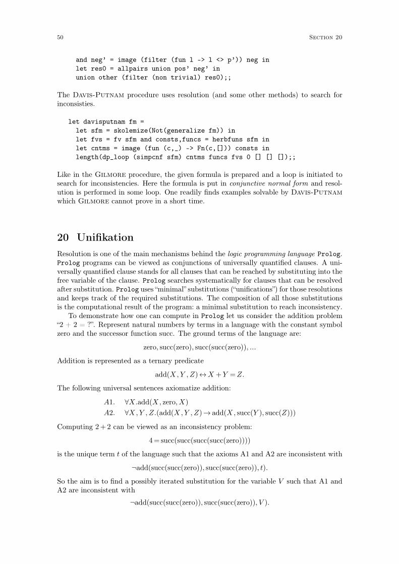
and neg’ = image (filter (fun l -> l <> p’)) neg in
let res0 = allpairs union pos’ neg’ in
union other (filter (non trivial) res0);;
The Davis-Putnam procedure uses resolution (and some other methods) to search forinconsisties.
let davisputnam fm =
let sfm = skolemize(Not(generalize fm)) in
let fvs = fv sfm and consts,funcs = herbfuns sfm in
let cntms = image (fun (c,_) -> Fn(c,[])) consts in
length(dp_loop (simpcnf sfm) cntms funcs fvs 0 [] [] []);;
Like in the Gilmore procedure, the given formula is prepared and a loop is initiated tosearch for inconsistencies. Here the formula is put in conjunctive normal form and resol-ution is performed in some loop. One readily finds examples solvable by Davis-Putnam
which Gilmore cannot prove in a short time.
20 Unifikation
Resolution is one of the main mechanisms behind the logic programming language Prolog.Prolog programs can be viewed as conjunctions of universally quantified clauses. A uni-versally quantified clause stands for all clauses that can be reached by substituting into thefree variable of the clause. Prolog searches systematically for clauses that can be resolvedafter substitution. Prolog uses “minimal” substitutions (“unifications”) for those resolutionsand keeps track of the required substitutions. The composition of all those substitutionsis the computational result of the program: a minimal substitution to reach inconsistency.
To demonstrate how one can compute in Prolog let us consider the addition problem“2 + 2 = ?”. Represent natural numbers by terms in a language with the constant symbolzero and the successor function succ. The ground terms of the language are:
zero, succ(zero), succ(succ(zero)), ...
Addition is represented as a ternary predicate
add(X, Y , Z)↔X +Y =Z.
The following universal sentences axiomatize addition:
A1. ∀X.add(X, zero, X)
A2. ∀X,Y , Z.(add(X,Y , Z)→ add(X, succ(Y ), succ(Z)))
Computing 2+2 can be viewed as an inconsistency problem:
4= succ(succ(succ(succ(zero))))
is the unique term t of the language such that the axioms A1 and A2 are inconsistent with
¬add(succ(succ(zero)), succ(succ(zero)), t).
So the aim is to find a possibly iterated substitution for the variable V such that A1 andA2 are inconsistent with
¬add(succ(succ(zero)), succ(succ(zero)), V ).
50 Section 20
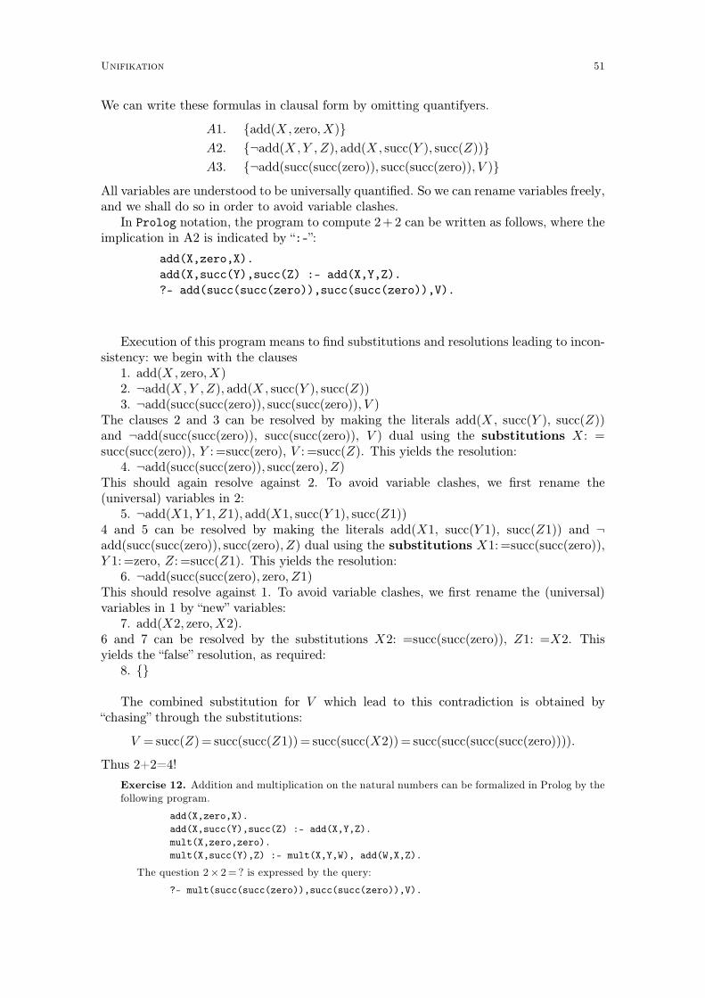
We can write these formulas in clausal form by omitting quantifyers.
A1. {add(X, zero, X)}
A2. {¬add(X,Y , Z), add(X, succ(Y ), succ(Z))}
A3. {¬add(succ(succ(zero)), succ(succ(zero)), V )}
All variables are understood to be universally quantified. So we can rename variables freely,and we shall do so in order to avoid variable clashes.
In Prolog notation, the program to compute 2+2 can be written as follows, where theimplication in A2 is indicated by “:-”:
add(X,zero,X).
add(X,succ(Y),succ(Z) :- add(X,Y,Z).
?- add(succ(succ(zero)),succ(succ(zero)),V).
Execution of this program means to find substitutions and resolutions leading to incon-sistency: we begin with the clauses
1. add(X, zero,X)2. ¬add(X, Y ,Z), add(X, succ(Y ), succ(Z))3. ¬add(succ(succ(zero)), succ(succ(zero)), V )
The clauses 2 and 3 can be resolved by making the literals add(X, succ(Y ), succ(Z))and ¬add(succ(succ(zero)), succ(succ(zero)), V ) dual using the substitutions X: =succ(succ(zero)), Y : =succ(zero), V : =succ(Z). This yields the resolution:
4. ¬add(succ(succ(zero)), succ(zero), Z)This should again resolve against 2. To avoid variable clashes, we first rename the(universal) variables in 2:
5. ¬add(X1, Y 1, Z1), add(X1, succ(Y 1), succ(Z1))4 and 5 can be resolved by making the literals add(X1, succ(Y 1), succ(Z1)) and ¬add(succ(succ(zero)), succ(zero), Z) dual using the substitutions X1:=succ(succ(zero)),Y 1:=zero, Z: =succ(Z1). This yields the resolution:
6. ¬add(succ(succ(zero), zero, Z1)This should resolve against 1. To avoid variable clashes, we first rename the (universal)variables in 1 by “new” variables:
7. add(X2, zero, X2).6 and 7 can be resolved by the substitutions X2: =succ(succ(zero)), Z1: =X2. Thisyields the “false” resolution, as required:
8. {}
The combined substitution for V which lead to this contradiction is obtained by“chasing” through the substitutions:
V = succ(Z)= succ(succ(Z1))= succ(succ(X2))= succ(succ(succ(succ(zero)))).
Thus 2+2=4!
Exercise 12. Addition and multiplication on the natural numbers can be formalized in Prolog by the
following program.
add(X,zero,X).
add(X,succ(Y),succ(Z) :- add(X,Y,Z).
mult(X,zero,zero).
mult(X,succ(Y),Z) :- mult(X,Y,W), add(W,X,Z).
The question 2× 2= ? is expressed by the query:
?- mult(succ(succ(zero)),succ(succ(zero)),V).
Unifikation 51
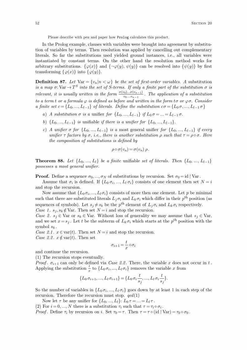
Please describe with pen and paper how Prolog calculates this product.
In the Prolog example, clauses with variables were brought into agreement by substitu-tion of variables by terms. Then resolution was applied by cancelling out complementaryliterals. So far the substitutions used yielded ground instances, i.e., all variables wereinstantiated by constant terms. On the other hand the resolution method works forarbitrary substitutions. {ϕ(x)} and {¬ϕ(y), ψ(y)} can be resolved into {ψ(y)} by firsttransforming {ϕ(x)} into {ϕ(y)}.
Definition 87. Let Var = {vn|n < ω} be the set of first-order variables. A substitutionis a map σ:Var→ T S into the set of S-terms. If only a finite part of the substitution σ is
relevant, it is usually written in the formσ(v0)...σ(vn−1)
v0....vn−1. The application of a substitution
to a term t or a formula ϕ is defined as before and written in the form tσ or ϕσ. Considera finite set c= {L0, ..., Ll−1} of literals. Define the substitution cσ= {L0σ , ..., Ll−1σ}
a) A substitution σ is a unifier for {L0, ..., Ll−1} if L0 σ= ...=Ll−1σ.
b) {L0, ..., Ll−1} is unifiable if there is a unifier for {L0, ..., Ll−1}.
c) A unifier σ for {L0, ..., Ll−1} is a most general unifier for {L0, ..., Ll−1} if everyunifier τ factors by σ, i.e., there is another substitution ρ such that τ = ρ ◦σ. Herethe composition of substitutions is defined by
ρ ◦σ(vn)=σ(vn) ρ .
Theorem 88. Let {L0, ..., Ll} be a finite unifiable set of literals. Then {L0, ..., Ll−1}possesses a most general unifier.
Proof. Define a sequence σ0, ..., σN of substitutions by recursion. Set σ0= id ↾Var .Assume that σi is defined. If {L0 σi, ..., Ll σi} consists of one element then set N = i
and stop the recursion.Now assume that {L0σi, ...,Llσi} consists of more then one element. Let p be minimal
such that there are substituted literals Ljσi and Lkσi which differ in their pth position (as
sequences of symbols). Let sj=/ sk be the pth element of Ljσi and Lkσi respectively.Case 1 . sj , sk∈/ Var. Then set N = i and stop the recursion.Case 2 . sj ∈ Var or sk ∈ Var. Without loss of generality we may assume that sj ∈ Var,and we set x= sj . Let t be the subterm of Lkσi which starts at the pth position with thesymbol sk .Case 2.1 . x∈ var(t). Then set N = i and stop the recursion.Case 2.2 . x∈/ var(t). Then set
σi+1=t
x◦σi
and continue the recursion.(1) The recursion stops eventually.Proof . σi+1 can only be defined via Case 2.2 . There, the variable x does not occur in t .Applying the substitution
t
xto {L0 σi, ..., Llσi} removes the variable x from
{L0 σi+1, ..., Llσi+1}= {L0 σit
sj, ..., Llσi
t
sj}.
So the number of variables in {L0σi, ..., Llσi} goes down by at least 1 in each step of therecursion. Therefore the recursion must stop. qed(1)
Now let τ be any unifier for {L0, ..., Ll}: L0 τ = ...=Ll τ .(2) For i=0, ..., N there is a substitution τi such that τ = τi ◦σi .Proof . Define τi by recursion on i. Set τ0= τ . Then τ = τ ◦ (id ↾Var)= τ0 ◦σ0 .
52 Section 20
Assume that τi is defined such that τ = τi ◦ σi and that i < N . Then σi+1 is definedaccording to Case 2.2 . With the notations of that case: σi+1=
t
x◦σi . Since τ = τi◦σi is a
unifier for {L0, ..., Ll} then τi is a unifier for {L0σi, ..., Llσi}. Thus the variable x and theterm t are unified by τi : xτi= τi(x)= tτi . Set
τi+1=(τi \ {(x, τi(x))})∪ {(x, x)}.
We show that τi+1 ◦t
x= τi : if y=/ x then
yt
xτi+1= yτi+1= yτi ,
if y=x then
yt
xτi+1= tτi+1= tτi (since x does not occur in t)=xτi= yτi .
Then
τi+1 ◦σi+1 = τi+1 ◦ (t
x◦σi)
= (τi+1 ◦t
x) ◦σi
= τi ◦σi
= τ .
�
We can now define first-order resolution.
Definition 89. Let c′ and c′′ be clauses. Let the substitutions σ ′: Var ↔ Var and σ ′′:Var↔Var be renamings of variables so that c′σ ′ and c′′σ ′′ do not have common variables.Let {L1, ..., Lm}⊆ c′σ ′ and {K1, ...,Kn}⊆ c′′σ ′′ be sets of literals such that
{L1, ..., Lm, K̄1, ..., K̄n}
is unifiable where m, n> 1 . Let σ be a most general unifier of {L1, ..., Lm, K̄1, ..., K̄n}.Then the clause
c= [(c′σ ′ \ {L1, ..., Lm})∪ (c′′σ ′′ \ {K1, ..., Kn})] σ
is a (first-order) resolution of c′ and c′′.
Given the clauses c′ and c′′ one just has to find parts which are unifiable and compute c .It is not necessary to “find” ground instances of the clauses. On the other hand, resolutionwith ground instances can be gotten from first-order resolution by lifting-techniques.
Theorem 90. Let c′ and c′′ be clauses and let c0′ and c0
′′ be ground instances of c′ andc′′ which are resolvable. Let c0 be a resolution of c0
′ and c0′′. Then there is a first-order
resolution c of c′ and c′′ such that c0 is a ground instance of c .
Proof. First let σ ′:Var↔ Var and σ ′′: Var↔ Var be renamings of variables so that c′σ ′
and c′′σ ′′ do not have common variables. Since c0′ and c0
′′ are ground instances of c′ andc′′ they are also ground instances of c′σ ′ and c′′σ ′′. Let
c0′ = c′σ ′τ ′ and c0
′′= c′′σ ′′τ ′′.
Since c′σ ′ and c′′σ ′′ do not have common variables we can assume that τ ′ and τ ′′ substitutedisjoint sets of variables. Letting τ = τ ′ ◦ τ ′′ we get
c0′ = c′σ ′τ and c0
′′= c′′σ ′′τ .
Unifikation 53
Let the resolution c0 of c0′ and c0
′′ be based on the literal L: L∈ c0′ and L̄∈ c0
′′ and
c0= (c0′ \ {L})∪ (c0
′′ \ {L̄}).
The literal L is a ground instance of possibly several literals L1, ...,Lm∈ c′σ ′ by the groundsubstitution τ . Similarly the literal L̄ is a ground instance of possibly several literalsK1, ...,
Kn∈ c′′σ ′′ by the ground substitution τ . Now τ unifies {L1, ..., Lm, K̄1, ..., K̄n} into L. Bythe theorem on the existence of most general unifiers let σ be a most general unifier for
{L1, ..., Lm, K̄1, ..., K̄n}.
Then
c= [(c′σ ′ \ {L1, ..., Lm})∪ (c′′σ ′′ \ {K1, ..., Kn})] σ
is a (first-order) resolution of c′ and c′′. Since σ is most general, take another substitutionρ such that τ = ρ ◦σ. Then
c0 = (c0′ \ {L})∪ (c0
′′ \ {L̄})
= (c′σ ′τ \ {L})∪ (c′′σ ′′τ \ {L̄})
= [(c′σ ′ \ {L1, ..., Lm})∪ (c′′σ ′′ \ {K1, ..., Kn})]τ
= [(c′σ ′ \ {L1, ..., Lm})∪ (c′′σ ′′ \ {K1, ..., Kn})]σρ
= cρ
is a ground instance of c . �
Theorem 91. Let C be a set of clauses and let c0= cσ0 be a ground instance of c . ThenC ⊢ c0 by resolution with ground clauses iff there is are substitutions σ and τ such thatC ⊢ cσ can be shown by first-order resolution and c0= cστ .
21 Set theory
Almost all mathematical notions can be defined set-theoretically. Georg Cantor, thefounder of set theory, gave the following definition or description:
Unter einer Menge verstehen wir jede Zusammenfassung M von bestim-mten, wohlunterschiedenen Objekten m unsrer Anschauung oder unseresDenkens (welche die “Elemente” von M genannt werden) zu einem Ganzen.
Felix Hausdorff begins the Grundzüge der Mengenlehre with a concise description,which seems less dependent on human minds:
Eine Menge ist eine Zusammenfassung von Dingen zu einem Ganzen, d.h.zu einem neuen Ding.
The notion of set is adequately formalized in first-order axiom systems introduced byZermelo, Fraenkel and others. Together with the Gödel completeness theorem forfirst-order logic this constitutes a “formalistic” answer to the question “what is mathem-atics”: mathematics consists of formal proofs from the axioms of Zermelo-Fraenkel settheory.
Definition 92. Let ∈ be a binary infix relation symbol; read x∈ y as “x is an element ofy”. The language of set theory is the language {∈}. The formulas in L{∈} are called set
theoretical formulas or ∈-formulas. We write L∈ instead of L{∈}.
54 Section 21
The naive notion of set is intuitively understood and was used extensively in previouschapters. The following axioms describe properties of naive sets. Note that the axiomsystem is an infinite set of axioms. It seems unavoidable that we have to go back to somepreviously given set notions to be able to define the collection of set theoretical axioms -another example of the frequent circularity in foundational theories.
Definition 93. The axiom system ST of set theory consists of the following axioms:
a) The axiom of extensionality (Ext):
∀x∀y(∀z(z ∈x↔ z ∈ y)→ x≡ y)
- a set is determined by its elements, sets having the same elements are identical.
b) The pairing axiom (Pair):
∀x∀y∃z∀w (w ∈ z↔w≡x∨w≡ y).
- z is the unordered pair of x and y.
c) The union axiom (Union):
∀x∃y∀z(z ∈ y↔∃w(w ∈x∧ z ∈w))
- y is the union of all elements of x.
d) The powerset axiom (Pow):
∀x∃y∀z(z ∈ y↔∀w(w ∈ z→w ∈x))
- y consists of all subsets of x.
e) The separation schema (Sep) postulates for every ∈-formula ϕ(z, x1, ..., xn):
∀x1...∀xn∀x∃y∀z (z ∈ y↔z ∈x∧ ϕ(z, x1, ..., xn))
- this is an infinite scheme of axioms, the set z consists of all elements of x whichsatisfy ϕ.
f ) The replacement schema (Rep) postulates for every ∈-formula ϕ(x, y, x1, ..., xn):
∀x1...∀xn(∀x∀y∀y ′((ϕ(x, y, x1, ..., xn)∧ ϕ(x, y ′, x1, ..., xn))→ y≡ y ′)→
∀u∃v∀y (y ∈ v↔∃x(x∈u∧ ϕ(x, y, x1, ..., xn))))
- v is the image of u under the map defined by ϕ.
g) The foundation schema (Found) postulates for every ∈-formula ϕ(x, x1, ..., xn):
∀x1...∀xn(∃xϕ(x, x1, ..., xn)→∃x(ϕ(x, x1, ..., xn)∧∀x′(x′∈x→¬ϕ(x′, x1, ..., xn))))
- if ϕ is satisfiable then there are ∈-minimal elements satisfying ϕ.
The axiom of extensionality expresses that a set is only determined by its elements.There is no further structure in a set; the order or multiplicity of elements does not matter.The axiom of extensionality can also be seen as a definition of ≡ in terms of ∈ :
∀x∀y(x≡ y↔∀z(z ∈x↔ z ∈ y)).
The axioms b)−d) describe the basic set theoretic operations of forming two-element sets,unions, and power sets. The separation schema (“Aussonderung”) is the crucial axiom ofZermelo set theory. Gottlob Frege had used the more liberal comprehension schema
∀x1...∀xn∃y∀z (z ∈ y↔ϕ(z, x1, ..., xn))
Set theory 55
without restricting the variable z to some x on the right hand side. This however lead tothe famous Russell paradox and was thus inconsistent. Zermelo’s restriction apparentlyavoids contradiction.
The replacement schema was added by Abraham Fraenkel to postulate that func-tional images of sets are sets.
The foundation schema by Mirimanoff allows to carry out induction on the binaryrelation ∈ . To prove a universal property by contradiction one can look at a minimalcounterexample and argue that the property is inherited from the elements of a set to theset. The schema is used seldomly in mathematical practice, but it is very convenient forthe development of set theory.
Note that the axioms of ST do not require the existence of infinite sets, and indeed onecan easily build a canonical model of ST consisting only of finite sets. Such a model canbe defined over the structure N= (N,+, ·, 0, 1). The theory ST has the same strength asfirst-order Peano arithmetic (PA).
The theory would become much stronger, if the axiom of infinity (Inf) was added:
∃x(∃y (y ∈x∧∀z¬z ∈ y)∧∀y(y ∈ x→∃z(z ∈x∧∀w(w ∈ z↔w ∈ y∨w≡ y)))).
Intuitively, the closure properties of x ensure that x is infinite. The strengthened theoryis Zermelo-Fraenkel set theory (without the axiom of choice), which is usually takenas the universal foundation of mathematics. We work with the weaker theory ST, sincewe want to show the Gödel incompleteness theorems for ST, which are another versionof the usual incompleteness theorems for PA.
21.1 Class terms
Most of the axioms have a form like
∀x~∃y∀z (z ∈ y↔ ϕ).
Intuitively, y is the collection of sets z which satisfy ϕ. The common notation for that set is
{z |ϕ}.
This is to be seen as a term, which assigns to the other parameters in ϕ the value {z |ϕ}.Since the result of such a term is not necessarily a set we call such terms class terms . Itis very convenient to employ class terms within ∈-formulas. We view this notation as anabbreviation for “pure” ∈-formulas.
Definition 94. A class term is of the form {x|ϕ} where x is a variable and ϕ ∈ L∈. If{x|ϕ} and {y |ψ} are class terms then
− u∈ {x|ϕ} stands for ϕu
x;
− u= {x|ϕ} stands for ∀v (v ∈ u↔ ϕv
x);
− {x|ϕ}=u stands for ∀v (ϕv
x↔ v ∈u);
− {x|ϕ}= {y |ψ} stands for ∀v (ϕv
x↔ ψ
v
y);
− {x|ϕ}∈u stands for ∃v(v ∈u∧ v= {x|ϕ};
− {x|ϕ}∈ {y |ψ} stands for ∃v(ψv
y∧ v= {x|ϕ}.
In this notation, the separation schema becomes:
∀x1...∀xn∀x∃y y= {z |z ∈x∧ ϕ(z, x1, ..., xn)}.
56 Section 21
We shall further extend this notation, first by giving specific names to important formulasand class terms.
Definition 95.
a) ∅ := {x|x=/ x} is the empty set;
b) V := {x|x=x} is the universe.
We work in the theory ZF for the following propositions.
Proposition 96.
a) ∅∈V.
b) V ∈/ V (Russell’s antinomy).
Proof. a) ∅∈V abbreviates the formula
∃v(v= v ∧ v= ∅).
This is equivalent to ∃v v= ∅ which again is an abbreviation for
∃v ∀w (w ∈ v↔w=/ w).
Consider an arbitrary set x . Then the formula is equivalent to
∃v ∀w (w ∈ v↔w ∈x∧w=/ w).
This follows from the instance
∀x∃y∀z (z ∈ y↔z ∈x∧ z=/ z)
of the separation schema for the formula z=/ z .b) Assume that V ∈V . By the schema of separation
∃y y= {z |z ∈V ∧ z ∈/ z}.
Let y= {z |z ∈ V ∧ z ∈/ z}. Then
∀z (z ∈ y↔ z ∈V ∧ z ∈/ z).
This is equivalent to
∀z (z ∈ y↔ z ∈/ z).
Instantiating the universal quantifier with y yields
y ∈ y↔ y ∈/ y
which is a contradiction. �
We introduce further abbreviations. By a term we understand a class term or a variable,i.e., those terms which may occur in an extended ∈-formula. We also introduce boundedquantifiers to simplify notation.
Definition 97. Let A be a term. Then ∀x∈Aϕ stands for ∀x(x∈A→ ϕ) and ∃x∈Aϕ
stands for ∃x (x∈A∧ ϕ).
Definition 98. Let x, y, z, ... be variables and X, Y ,Z , ... be class terms. Define
a) X ⊆Y :=∀x∈X x∈Y, X is a subclass of Y ;
b) X ∪ Y := {x|x∈X ∨ x∈Y } is the union of X and Y ;
Set theory 57
c) X ∩ Y := {x|x∈X ∧ x∈Y } is the intersection of X and Y ;
d) X \Y := {x|x∈X ∧x∈/ Y } is the difference of X and Y ;
e)S
X := {x|∃y ∈X x∈ y} is the union of X ;
f )T
X := {x|∀y ∈X x∈ y} is the intersection of X ;
g) P(X)= {x|x⊆X} is the power class of X;
h) {X}= {x|x=X} is the singleton set of X;
i) {X,Y }= {x|x=X ∨ x= Y } is the (unordered) pair of X and Y;
j ) {X0, ..., Xn−1}= {x|x=X0∨ ...∨x=Xn−1}.
One can prove the well-known boolean properties for these operations. We only give afew examples.
Proposition 99. X ⊆ Y ∧ Y ⊆X→X = Y.
Proposition 100.S
{x, y}=x∪ y.
Proof. We show the equality by two inclusions:(⊆). Let u∈
S{x, y}. ∃v(v ∈{x, y}∧u∈ v). Let v∈ {x, y}∧u∈ v. (v=x∨ v= y)∧u∈ v.
Case 1 . v= x. Then u∈x. u∈x∨ u∈ y. Hence u∈x∪ y.Case 2 . v= y. Then u∈ y. u∈x∨u∈ y. Hence u∈x∪ y.
Conversely let u∈ x∪ y. u∈x∨u∈ y.Case 1 . u∈x. Then x∈ {x, y}∧u∈x. ∃v(v ∈ {x, y}∧u∈ v) and u∈
S{x, y}.
Case 2 . u∈ y. Then x∈ {x, y}∧ u∈x. ∃v(v ∈ {x, y}∧u∈ v) and u∈S
{x, y}. �
We can now reformulate the ZF axioms using class terms; for brevity we omit initialuniversal quantifiers.
a) Extensionality: x⊆ y ∧ y⊆ x→ x= y.
b) Pairing: {x, y}∈ V .
c) Union:S
x∈V .
d) Powerset: P(x)∈V .
e) Separation schema: for all terms A with free variables x0, ..., xn−1
x∩A∈V .
f) Replacement: see later.
g) Foundation: for all terms A with free variables x0, ..., xn−1
A=/ ∅→∃x∈A x∩A= ∅.
Also the axiom of infinity can be written as
∃x (∅∈ x∧∀u∈x u∪ {u}∈x).
22 Relations and functions
Ordered pairs are the basis for the theory of relations.
58 Section 22
Definition 101. (x, y)= {{x}, {x, y}} is the ordered pair of x and y .
Remark 102. There are sometimes discussions whether (x, y) is the ordered pair of x
and y , or to what degree it agrees with the intuitive notion of an ordered pair. ...
Proposition 103. (x, y)∈V.(x, y)= (x′, y ′)→x= y ∧x′= y ′.
Definition 104. Let A,B,R be terms. Define
a) A×B= {z |∃a∈A∃b∈B z= (a, b)} is the cartesian product of A and B .
b) R is a (binary) relation if R⊆V ×V.
c) If R is a binary relation write aRb instead of (a, b)∈R.
We can now introduce the usual notions for relations:
Definition 105.
a) dom(R)= {x|∃y (x, y)∈R} is the domain of R.
b) ran(R)= {y |∃x (x, y)∈R} is the range of R.
c) R ↾A= {z |z ∈R∧∃x∃y((x, y)= z ∧x∈A)} is the restriction of R to A.
d) R[A] = {y |∃x∈A xRy} is the image of A under R.
e) R−1= {z |∃x∃y (xRy∧z=(y, x))} is the inverse of R .
f ) R−1[B] = {x|∃y ∈B xRy} is the preimage of B under R .
One can prove the usual properties for these notions in ZF. One can now formalize thetypes of relations, like equivalence relations, partial and linear orders, etc. We shall onlyconsider notions which are relevant for our short introduction to set theory.
Definition 106. Let F ,A,B be terms. Then
a) F is a function if ∀x∀y, y ′ (xFy∧xFy ′→ y= y ′).
b) F : A → B if F is a function∧dom(F ) = A ∧ ran(F ) ⊆ B. The sequence notions(F (x)|x∈A) or (F (x))x∈A are just other ways to write F :A→V.
c) F (x)= {v |∃y (xFy∧∀y ′ (xFy ′→ y= y ′)→∃y (xFy∧v ∈ y)} is the value of F at x.
Note that if F :A→B and x∈A then xFF (x). If there is no unique y such that xFythen F (x)= V which we may read as F (x) is “undefined”.
Using functional notations we may now write the replacement schema as
F is a function → F [x]∈ V .
One could now develop the usual theory of functions and formalize notions like sur-jective, injective, bijective, compositions, etc.
23 Natural numbers and complete induction
It is natural to formalize the integer n in set theory by some set with n elements. Thisintuitive plan will be implemented in the sequel. For every ordinary natural number wedefine a set-theoretical version.
Natural numbers and complete induction 59
Definition 107.0 = ∅1 = {0}2 = {0, 1}
···n+1 = {0, 1, ..., n} = {0, 1, ..., n− 1}∪ {n} =n∪ {n}
···For x∈V define x+1=x∪ {x} and x+2= (x+1)+ 1.
We would like to set N= {0, 1, 2, ...}, but such infinitary definitions are not possiblein first-order logic. Instead we look for a characteristic property to define a class which isable to serve as the collection of set-theoretic integers. Every ordinary integer n is eitherof the form n=0 or n=m+1 for some other integer.
Definition 108. A set n is a natural number if
∀i∈n+1(i=0∨∃j ∈n.i= j+1).
Let N be the class of natural numbers. We shall often use letters like i, j , k, l, m, n asvariables for natural numbers.
We show that this class is an adequate formalization of the intuitive notion of “naturalnumber”.
Lemma 109.
a) 0∈N ;
b) ∀n∈N. n+1∈N ;
c) 0, 1, 2, ...∈N .
Proof. a) is trivial. b) Assume n ∈N .To show that n+ 1 ∈N consider i ∈ (n+ 1) + 1=(n+1)∪ {n+1}. If i∈n+1 then we have by assumption that i=0∨∃j ∈n.i= j+1 andso i=0∨∃j ∈n+1.i= j +1. If i=n+1 then n∈n+1 satisfies ∃j ∈n+1.i= j+1. �
N is the ⊆-smallest class which contains 0 and is closed under +1.
Lemma 110. Let A be a term such that 0∈A and ∀x∈A.x+1∈A . Then N⊆A .
Proof. Let n ∈N . Assume for a contradiction that n ∈/ A . By foundation let i ∈ n+ 1be ∈-minimal such that i∈/ A . Then i=/ 0 . By the definition of N there is j ∈n such thati= j+1 . Then j ∈ i and by the ∈-minimality of i we have j ∈A . But then i= j+1∈A .Contradiction. �
This immediately implies the principle of (complete) induction theorem for naturalnumbers.
Theorem 111. Let ϕ(n, p~) be an ∈-formula. Assume that ϕ(0, p~) and that ∀n∈N.ϕ(n,p~)→ ϕ(n+1, p~). Then ∀n∈N.ϕ(n, p~).
Proof. Apply the previous lemma with A= {x∈N | ϕ(x, p~)}. �
Theorem 112. N is a set if the axiom of infinity holds.
60 Section 23
Proof. If the axiom of infinity holds, take a set x such that
(∃y (y ∈x∧∀z¬z ∈ y)∧∀y(y ∈x→∃z(z ∈x∧∀w(w ∈ z↔w ∈ y ∨w≡ y)))).
This means that ∅∈x∧∀y ∈x.y+1∈x . By Lemma 110, N⊆x . Then N=x∩N is a setby separation.
Conversely assume that N∈V . Then N obviously witnesses the axiom of infinity. �
So the axiom of infinity can be written briefly as
N∈V .
The natural numbers are linearly ordered by ∈ . To prove this we draw a useful consequenceof foundation, which also shows that the ∈-relation is strict on N .
Lemma 113. There is no finite sequence x0, x1, ..., xn which forms an ∈-cycle with
x0∈x1∈ ...∈ xn∈x0 .
In particular ∀xx∈/ x .
Proof. Assume that x0∈ x1∈ ...∈ xn∈ x0 . Let A= {x0, ..., xn}. A=/ ∅ since x0∈A . Byfoundation, take x∈A such that x∩A= ∅ .Case 1 . x=x0 . Then xn∈x∩A=/ ∅ , contradiction.Case 2 . x=xi for some 16 i6n . Then xi−1∈x∩A= ∅ , contradiction. �
Theorem 114. ∀m,n∈N.m∈n∨m=n∨n∈m .
Proof. By complete induction on m∈N . The property holds for m=0(1) ∀n∈N.0∈n∨ 0=n∨n∈ 0 .Proof . By complete induction on n∈N . The initial case n=0 is trivial:(1.1) 0∈ 0∨ 0= 0∨ 0∈ 0.(1.2) Assume that 0∈n∨ 0=n∨n∈ 0. Then 0∈n+1∨ 0=n+1∨n+1∈ 0.Proof . We have 0∈n∨ 0=n . Then 0∈n+1 . qed(1.2, 1)(2) Assume ∀n∈N.m∈n∨m=n∨n∈m . Then ∀n∈N.m+1∈n∨m+1=n∨n∈m+1 .Proof . We prove the conclusion by induction on n∈N .(2.1) m+1∈ 0∨m+1=0∨ 0∈m+1 .Proof . By assumptionm∈0∨m=0∨0∈m . Then 0∈m∨0=m . Thus 0∈m+1 . qed(2.1)(2.2) Assume that m+1∈n∨m+1=n∨n∈m+1 . Then m+1∈n+1∨m+1=n+1∨n+1∈m+1 .Proof . If m+1∈n∨m+1=n then m+1∈n+1 as required. So assume that n∈m+1 .If n=m then m+1=n+1 as required.
This leaves the case n∈m . By the assumption of (2) we have m∈n+1∨m=n+1∨n+1 ∈m. We obtain a contradiction from the case m ∈ n+ 1: if m ∈ n then m ∈ n ∈m ,contracting the previous lemma; if m=n then m∈m which again contradicts the lemma.So we are left with m=n+1∨n+1∈m which implies n+1∈m+1 . qed(2.2, 2) �
Definition 115. Let <= {(m,n)|m∈n} be the natural strict linear order on N .
A natural number is the set of smaller numbers.
Lemma 116. For n∈N, n⊆N . Therefore n= {m∈N |m<n}.
Proof. By induction on n ∈ N . Obviously ∅ ⊆ N . Assume that n ⊆ N . Then n + 1 =n∪ {n}⊆N . �
Natural numbers and complete induction 61
So, intuitively, we have the desired n= {0, 1, ..., n− 1}.
24 Complete recursion and arithmetic
Recursion, often called induction as well, over the natural numbers is a ubiquitous methodfor defining mathematical objects.
Theorem 117. Let a∈V and G:V →V. Then there is a canonically defined class term F
such that
F :N→V , F (0)= a and ∀n∈N F (n+1)=G(F (n)).
We then say that F is defined by recursion over N by the recursion equations F (0)=a and∀n∈N F (n+1)=G(F (n)). Moreover, the function F is uniquely determined: if F ′:N→V
satisfies the recursion equations F ′(0)= a and ∀n∈N F ′(n+1)=G(F ′(n)) then F =F ′.
Proof. To “compute” the value of F at some k∈N we would intuitively form a sequence of(F (0),F (1), ...,F (k)) according to the recursion equations. This finite sequence is uniquelydetermined by k .(1) For all k∈N there exists a unique f :k+1→V such that f(0)=a and ∀n<k.f(n+1)=G(f(n)).Proof . By induction on k . For k=0 set f = {(0, a)}: 1→V . Obviously, this f is uniquelydetermined.
Assume that k ∈ N and that f : k + 1 → V is the uniquely determined function withf(0)= a and ∀n<k.f(n+1)=G(f(n)). Define
f ′= f ∪ {(k+1, G(f(k)))}: k+2→V .
Then f ′ ∈ V is a set by pairing and union. Also f ′(0) = a and ∀n < k + 1. f ′(n + 1) =G(f ′(n)) by the assumptions on f and by the definition of f ′.
Consider some f ′′:k+2→V such that f ′′(0)=a and ∀n<k+1. f ′′(n+1)=G(f ′′(n)).By the uniqueness assumption at k we must have f ′′ ↾ k+1= f = f ′ ↾ k+1 . Also
f ′′(k+1)=G(f ′′(k))=G(f(k))=G(f ′(k))= f ′(k+1).
Thus f ′′= f ′ which proves uniqueness at k+1 . qed(1)We can now define
F = {(k, f(k))| k ∈N∧ f : k+1→V ∧ f(0)= a∧∀n<k.f(n+1)=G(f(n))}.
By (1), F :N→V , and we have to check the recursive equations. F (0)= f(0)=a for someappropriate f . For n∈N choose f :n+2→V with f(0)= a∧∀k <n.f(k+1)=G(f(k)).As before, f ↾n+1 is the unique function used to define F (n). Then
F (n+1)= f(n+1)=G(f(n))=G((f ↾n+1)(n))=G(F (n)).
Finally, to show the uniqueness of F let F ′:N→V satisfy the recursion equations F ′(0)=a
and ∀n∈N F ′(n+1)=G(F ′(n)).(2) ∀n∈N.F (n)=F ′(n).Proof . By induction. F (0)=a=F ′(0). For the induction step assume that F (n)=F ′(n).Then F (n+1)=G(F (n))=G(F ′(n))=F ′(n+1). �
We can now define arithmetical operations on natural numbers, using familiar recursiveproperties.
62 Section 24
Definition 118. Define the sum add(m, n) of m, n ∈ N by recursion on the variable n
(taking m as a parameter) such that
add(m,n)=
�m, if n=0add(m, k)+ 1, if n= k+1
Also write m+n instead of add(m,n). Then the recursive equation can be written as
m+0 = m
m+(n+1) = (m+n)+ 1 .
One can show that addition satisfies the expected properties.
Proposition 119.
a) m+n∈N .
b) m+0=0+m=m .
c) (i+ j)+ k= i+ (j+ k).
d) m+n=n+m .
Proof. By induction. �
Definition 120. Define the product m ·n of m,n∈N:
m · 0 = 0
m · (n+1) = (m ·n)+m
Multiplication satisfies natural properties.
Proposition 121.
a) m ·n∈N .
b) m · 0=0 ·m=0 .
c) (k ·m) · l= k · (m · l).
d) k · (l+m)= (k · l)+ (k ·m).
e) m ·n=n·m .
Proof. By induction. �
Definition 122. Define the power mn of m,n∈N recursively:
m0 = 1
mn+1 = (mn) ·m
Again one can prove the usual arithmetic laws for exponentiation. We shall also needthat obvious instances of these laws are provable in ST. E.g.,
a) ST⊢ 0< 1, ST⊢ 0< 2, ST⊢ 1< 2, etc.. To interpret these statements observe thatthe formulas on the right-hand side of ⊢ have to be ∈-formulas. Hence the “numbers”occuring in those formulas must be abstraction terms, i.e., they are the set-theoreticnumbers defined by 0=∅ and n+1=n∪{n}, and the <-symbol is the set-theoretic∈. To prove that, e.g., ST ⊢ 3 < 5 requires in principle to unravel the abstractionterm notation into ∈-notation. Although these proof are schematic, ST⊢ 3< 5 willbe proved by a different and much shorter proof than ST⊢ 121< 122 .
Complete recursion and arithmetic 63
b) In the metatheory, where we are constructing statements and proofs, these consid-eration can be expressed by:
if m and n are ordinary natural numbers withm<n then ST⊢m<n .
This metatheoretic statement deserves some comment: it is a universal statementin the metatheory, quantifying over all ordinary natural numbers, i.e., the intuitivemathematical numbers. In the metatheory we can form the set-theoretic statementm<n for all ordinary natural numbersm and n. The statement ST⊢m<n containsa metatheoretic existential quantification expressing that a formal proof exists.
25 Formalizing the metatheory in the object theory
We are currently “reflecting” parts of our metatheory, i.e., common mathematical argu-mentation, into our object theory ST. So far this has been done for class operations,ordered pairs, relations, functions, and natural numbers. We have given ST-definitions ofcertain notions and we have proved propositions showing that the ST-definitions satisfyST-properties corresponding to properties of the original metatheoretic notions. If the ST-definitions are chosen efficiently then the proofs of the propositions should be straightfor-ward, corresponding to the usual intuitions and arguments.
We shall continue to formalize the syntax of first-order logic within ST. To avoid confu-sion, it is helpful to distinguish between metatheoretic notions and their ST-formalizations.We introduce “Gödel brackets” to denote formalizations.
If A is a metatheoretic notion that has been formalized in ST we mayuse ⌈A⌉ to denote its formalization.
Sometimes ⌈A⌉ is called the Gödelization of A . If we would formalize into numbertheory instead of set theory, and if then ⌈A⌉ is a natural number, one often calls ⌈A⌉ theGödel number of A . Analogously we may call ⌈A⌉ the Gödel set of A . This turns propertiesof mathematical objects into properties of sets.
So in defining the natural numbers within ST we could have been more careful bydefining⌈0⌉ = ∅⌈1⌉ = {0}⌈2⌉ = {0, 1}
···⌈n+1⌉ = {0, 1, ..., n} = {0, 1, ..., n− 1}∪ {n} =n∪ {n}
···Then the “correctness” statements from the last chapter look like:
a) ST ⊢⌈ 0⌉ <⌈ 1⌉, ST ⊢⌈ 0⌉ <⌈ 2⌉, ST ⊢⌈ 1⌉ <⌈ 2⌉, etc.. That < is the set-theoretic<-relation, namely ∈, can still be infered from the context. Of course one couldalso introduce further notation to distinguish the set-theoretic relation from themetatheoretic <-relation. We shall, however, try to restrict our notation to thenecessary.
b) if m and n are ordinary natural numbers with m<n then ST⊢⌈m⌉<⌈n⌉ .
There are many more correctness statements in the context of our formalizations. If theformalization was to be carried out in some automatic system, one should introduce mech-anisms to prove most of these schematically and automatically. Here some examples:
a)
64 Section 25
if k · l=m then ST⊢⌈ k⌉ ·⌈ l⌉=⌈m⌉
if k · l=/ m then ST⊢⌈ k⌉ ·⌈ l⌉=/ ⌈m⌉
The implications of a) cannot be reversed (at the moment). We cannot argue that
warning: if ST⊢⌈ k⌉ ·⌈ l⌉=⌈m⌉ then k · l=m .
The reason is that ST, for all we know, might be an inconsistent theory so that STwould be able to prove every statement of set theory. There are difficult relations between
truth (“m<n”) and provability (“ST⊢⌈m<n⌉”) which also concern the mechanics behindthe Gödel incompleteness theorems.
26 Finite sequences
For the incompleteness results we want to formalize first-order syntax within ST. Syntaxis very much about finite sequences: words are finite sequences of symbols, sequents arefinite sequences of formulas, formal derivations are finite sequences of sequents. Carryingout syntax within ST requires a good theory of finite sequences within ST. For the nextdefinition observe that a set-theoretical natural number is equal to the set of all smallernumbers.
Definition 123. w is a finite sequence if w:n→V for some n∈N. We call n the lengthof w and write length(w)=n or |s|=n . For i< |s| write wi instead of w(i). The sequences will also be denoted by (wi)i<n , (w0, ..., wn−1) or w0...wn−1 .
Let V ∗ be the class of all finite sequences. For sequences w=w0...wm−1 and w0′ ...wn−1
′
define the concatenation w
˘w ′ to be the unique sequence with length(w
˘w ′)=m+n and
(w˘w ′)i=
(
wi , for i <m
wi−m′ , for m6 i <m+n
We also write w0...wm−1w0′ ...wn−1
′ or ww ′ instead of w˘w ′.
Lemma 124. V ∗ with˘has the properties of a monoid with cancellation:
a)˘is associative: (ww ′)w ′′=w(w ′w ′′).
b) ∅ is a neutral element for˘: ∅w=w∅=w.
c)˘satisfies cancelation: if uw=u′w then u=u′; if wu=wu′ then u=u′.
Exercise 13. Prove these laws by induction.
The associative law allows us to omit brackets in multiple concatenations and to writeww ′ w ′′ instead of (ww ′) w ′′. We can also view “single” sets s as sequences of length 1 ,writing simply s instead of (s); then ws stands for w
˘(s).
Finite sequences can be used to define “smallest” classes closed under given functions.Let us first introduce multi-argument functions.
Definition 125. For a term A and n∈N let
An= {w |w:n→A}
be the n-fold cartesian product of A. F :An→V is called an n-ary function on A.
Finite sequences 65
Note that ∅: 0→V and A0= {∅}. So a 0-ary function F :V 0→V can be identified withits constant value F (∅).
Exercise 14. Show in ST that xn∈V .
26.1 Calculi
We have defined terms and formulas of first-order logic as calculi that produced, e.g.,formulas out of other formulas and out of other syntactic material. We had used the meta-mathematical definition:
Definition 126. The class LS of all S-formulas is the smallest subclass of S∗ such that
a) ⊥∈LS (the false formula);
b) t0≡ t1∈LS for all S-terms t0, t1∈T S (equality);
c) Rt0...tn−1∈LS for all n-ary relation symbols R∈S and all S-terms t0, ..., tn−1∈TS
(relational formula);
d) ¬ϕ∈LS for all ϕ∈LS (negation);
e) (ϕ→ ψ)∈LS for all ϕ, ψ ∈LS (implication);
f ) ∀xϕ∈LS for all ϕ∈LS and all variables x (universalisation).
We want to capture these formation rules by a single function F such that
a) (0)7→F⊥ ;
b) (1, t0, t1)7→Ft0≡ t1 for t0, t1∈ TS ;
c) (2, R, t0, ..., tn−1)7→FRt0...tn−1 for R∈S an n-ary relation symbol;
d) (3, ϕ)7→F¬ϕ ;
e) (4, ϕ, ψ) 7→F(ϕ→ ψ) ;
f) (5, x, ϕ) 7→F∀xϕ for x∈Var .
The first element of the arguments signifies which formation rule is to be used; the furtherarguments consist of “previously formed” formulas and other material. We now prove thatthe smallest class closed under F can be expressed in ST.
Theorem 127. Let F :D→V be given. A term B is called F-closed if whenever (z, s)∈D
and s∈B∗ then F (z,s)∈B. Then we can canonically define a class AF which is the uniquelydetermined ⊆-minimal F-closed class: if B is another F-closed term then AF ⊆B. We callA the class generated by F, or the smallest class such that ... , where ... stands for theproperties that define F as in the example above.
An F-derivation of x∈AF is a finite sequence f :n+1→V such that
∀m6n∃(z, s)∈D.s∈ (f [m])∗∧ f(m)=F (z, s)∧ f(n)= x.
We view F as a generating function: if F (x, s) = t and s = (s0, ..., sn−1) is a finitesequence then we can view t as being built from s0, ..., sn−1 , possibly using the extramaterial x . An F -derivation is a finite sequences in which every step is generated fromearlier steps using F .
66 Section 26
Proof. Set
A= {x|∃n∈N∃f :n+1→V .f is an F -derivation of x}.
(1) A is F -closed.Proof . Let (y, t)∈D with t∈A∗. We have to show that x=F (y, t)∈A . Take k ∈N suchthat t=(t0, ..., tk−1)∈Ak. For l < k take an F -derivation fl:nl+1→V of tl .
Then
f = f0
˘f1
˘...
˘fk−1
˘(x): 1+
X
l<k
(nl+1)→V
is an F -derivation of x . qed(1)(2) Let B be F -closed. Then A⊆B.Proof . Let f :n+1→V be an F -derivation. It suffices to prove by induction on n′6n that∀m6n′. f(m)∈B . For n′=0 and m=0 there is some (z, s)∈D such that s∈ (f [0])∗={∅}and f(0)=F (z, ∅). ∅∈B0 and by the assumptions on B
f(0)=F (z, ∅)∈B.
For the induction step consider n′+16 n and assume that ∀m6n′. f(m)∈B. It sufficesto see that f(n′+1)∈B . Set m=n′+1 . Take some (z, s)∈D such that s∈ (f [m])∗ andf(m)=F (z, s). By the inductive assumption s∈B∗ and by the assumptions on B
f(m)=F (z, s)∈B.
�
The class A generated by F~ can be seen as a least fixed point with respect to a certainclosure under F . In the above construction, A is reached via derivations “from below”. Ifthere is some F -closed set z0 then the fixed point can also be reached by intersections “fromabove”:
A=\
{y |y is F -closed}.
The intersection on the right-hand side is non-trivial since z0 is a factor of the intersection.
26.2 Gödelization of finite sequences
We want to Gödelize the syntactic notions of first-order logic. In the meta-theory theseare defined using finite sequences. Therefore we have to Gödelize finite sequences.
Definition 128. Let w=w0...wn−1 be a meta-theoretic finite sequence of objects wi which
possess a Gödelization ⌈wi⌉. Then the Gödelization of w is defined as
⌈w⌉=�
⌈w0⌉, ..., ⌈wn−1
⌉ �.
One can show some correctness properties by meta-theoretic induction.
Proposition 129.
a) ⌈w0...wn−1u0...um−1⌉
=⌈w0...wn−1⌉
˘⌈u0...um−1
⌉
b) ...
26.3 Finite and infinite sets
Finite sequences can also be used to formalize the notions of finite and infinite.
Finite sequences 67
Definition 130. A set x is finite if there is a finite sequence f ∈V ∗ such that x= ran(f).For a finite set x define its cardinality by
card(x)= x̄̄=min {n|∃f :n→ x.x= ran(f)}
A set x is infinite if it is not finite.
Lemma 131.
a) ∅ is finite with card(∅)= 0.
b) {x} and {x, y} are finite with card({x})= 1, and card({x, y})= 2 iff x=/ y.
c) If x is finite and every element of x is finite thenS
x is finite.
d) If x is finite and y⊆ x then y is finite with card(y)6 card(x).
e) If x and y are finite then x ∪ y is finite with card(x ∪ y) = card(x) + card(y) −card(x∩ y).
f ) If x is finite then P(x) is finite with card(P(x))= 2card(x).
g) If F is a function and x is finite then F [x] is finite with card(F [x])6 card(x).
h) every n∈N is finite with card(n)=n.
i) If N∈ V then N is infinite.
Exercise 15. Prove the Lemma.
27 Formalizing syntax within ST
We now carry out the syntactic definitions of first-order logic within ST.
Definition 132. Set
a) ⌈≡⌉=8801 (equality),
b) ⌈¬⌉=172 (negation),
c) ⌈→⌉=8594 (implication),
d) ⌈⊥⌉=8869 (false),
e) ⌈∀⌉=8704 (universal quantifier),
f ) ⌈(⌉=40 (left bracket),
g) ⌈ )⌉=41 (right bracket),
h) vn=(0, n, 0) for n∈N (the n-th variable),
i) an n-ary relation symbol is a triple of the form R=(1, x, n) with x∈V and n∈N,
j ) an n-ary function symbol is a triple of the form f = (2, x, n) with x∈V and n∈N.
k) Let Var= {vn|n∈N} be the class of variables.
l) Let S0= { ⌈≡⌉ ,⌈¬⌉ , ⌈→⌉ ,⌈⊥⌉ , ⌈∀⌉ , ⌈(⌉ ,⌈�⌉ }∪Var be the class of basic symbols.
m) A term S is a language if every s∈S is a relation symbol or a function symbol.
68 Section 27
Note that the basic symbols, the relation symbols, and the function symbols are allpairwise distinct. We also have an unlimited supply of relation and function symbols. The(set-theoretic) numbers that we have chosen for the symbols ≡,¬, ... are their numbers inthe Unicode font. This choice is in principle rather arbitrary. It is often convenient to usethe metatheoretic symbols ≡, ¬, ... as abbreviations for their Gödelizations. So (v3 ≡ v4)is a formula in the language of set theory, and at the same time it denotes a unique classterm which is the finite sequence
(v3≡ v4) = ((, v3,≡, v4, ))
= (40, (0, 3, 0), 8801, (0, 4, 0), 41)
We have encoutered such “overloading” of notation already with other set-theoretic form-alizations: 5 can denote the meta-theoretic number “five” or the class term 5. Whether(v3≡ v4) is to be read as an ∈-formula or as a settheoretic term should be derivable fromthe context. Simple meta-theoretic properties should, however, “reflect” from the meta-theory into ST:
if vn∈Var then ST⊢ vn∈Var .
”vn∈Var” on the left-hand side is a meta-theoretical syntactical property. ”vn∈Var” on theright-hand side is an ∈-formula which can be proved in ST, due to the simple definition ofthe term Var.
Definition 133. (In ST) Let S be a language. A word over S is a finite sequence
w:n→S0∪S.
for some number n∈N which is the length of w. Let S∗ be the class of all words over S.
Consider a meta-theoretic language S and let ⌈S⌉ be a “Gödelization” of S such thatfor every symbol s in S :
⌈s⌉∈⌈S⌉.
Then for every meta-theoretic word w over S we have
ST⊢⌈w⌉ is a word over⌈S⌉.
Definition 134. The class TS of all S-terms is the smallest subclass of S∗ such that
a) x∈TS for all variables x∈Var;
b) ft0...tn−1 ∈ TS for all n ∈N, all n-ary function symbols f = (2, y, n) ∈ S, and all
t0, ..., tn−1∈T S.
Let ⌈S⌉ be a “Gödelization” of S such that for every n-ary function symbol s in S :
⌈s⌉∈⌈S⌉ is of the form ⌈s⌉=(2, x,⌈n⌉).
In the above situation of the Gödelization of a language we have for every meta-theoreticS-term t that
ST⊢⌈ t⌉ is an ⌈S⌉-term.
This can be proved by a meta-theoretic induction on the length of derivations of t. TheGödelization of a derivation is again a derivation in ST, and every member of the derivationis an ⌈S⌉-term.
In ST one can prove the unique readability of terms.
Formalizing syntax within ST 69
Lemma 135. For every term t∈T S exactly one of the following holds:
a) t∈Var;
b) there is a uniquely defined function symbol f = (2, y, n)∈ S and a uniquely defined
sequence t0, ..., tn−1∈T S of terms such that t= ft0...tn−1 .
Definition 136. The class LS of all S-formulas is the smallest class such that
a) ⊥∈LS ;
b) t0≡ t1∈LS for all S-terms t0, t1∈T S ;
c) Rt0...tn−1∈LS for all n-ary relation symbols R=(1, y, n)∈S and all S-terms t0, ...,
tn−1∈ TS ;
d) ¬ϕ∈LS for all ϕ∈LS ;
e) (ϕ→ ψ)∈LS for all ϕ, ψ ∈LS ;
f ) ∀vnϕ∈LS for all ϕ∈LS and all vn=(0, n, 0)∈Var.
Assuming a “correct” Gödelization of the language S we have for every meta-theoreticS-formula ϕ that
ST⊢⌈ ϕ⌉ is an ⌈S⌉-formula.
And in ST one prove the unique readability of formulas. Then simple syntactic recursionscan be formalized in ST.
Definition 137. For t ∈ T S define var(t) ⊆ {vn|n ∈ N} by recursion on (the lengths of)terms:
− var(x)= {x};
− var(c)= ∅;
− var(ft0...tn−1)=S
i<n var(ti).
Definition 138. Für ϕ ∈ LS define the set of free variables free(ϕ) ⊆ {vn|n ∈ N} byrecursion on (the lengths of) formulas:
− free(t0≡ t1)= var(t0)∪ var(t1);
− free(Rt0...tn−1)= var( t0)∪ ...∪ var(tn−1);
− free(¬ϕ)= free(ϕ);
− free(ϕ→ ψ)= free(ϕ)∪ free(ψ).
− free(∀xϕ)= free(ϕ) \ {x}.
For Φ⊆LS define the class free(Φ) of free variables as
free(Φ)=[
ϕ∈Φ
free(ϕ) .
Definition 139. For a term s∈T S, pairwise distinct variables x0, ..., xr−1 and terms t0, ...,tr−1∈ TS define the (simultaneous) substitution
st0....tr−1
x0...xr−1
70 Section 27
of t0, ..., tr−1 for x0, ..., xr−1 by recursion:
a) xt0....tr−1
x0...xr−1=
�
x, if x=/ x0, ..., x=/ xr−1
ti , if x= xifor all variables x;
b) (fs0...sn−1)t0....tr−1
x0...xr−1= fs0
t0....tr−1
x0...xr−1...sn−1
t0....tr−1
x0...xr−1for all n-ary function symbols
f ∈S .
One can check again, that Gödelizations commute with forming the set of free variablesand with substitution.
Definition 140. A finite sequence (ϕ0, ...,ϕn−1,ϕn) of S-formulas is called a sequent. Theinitial segment Γ=(ϕ0, ...,ϕn−1) is the antecedent and ϕn is the succedent of the sequent.We usually write ϕ0 ...ϕn−1ϕn or Γϕn instead of (ϕ0, ...,ϕn−1,ϕn). To emphasize the lastelement of the antecedent we may also denote the sequent by Γ′ ϕn−1 ϕn with Γ′=(ϕ0, ...,
ϕn−2).
Again, if Γϕ is a meta-theoretic sequence then
ST⊢⌈Γϕ⌉ is a sequence.
Definition 141. The sequent calculus consists of the following (sequent-)rules:
− monotonicity (MR)Γ ϕ
Γ ψ ϕ
− assumption (AR)Γ ϕ ϕ
− →-introduction (→I)Γ ϕ ψ
Γ ϕ→ ψ
− →-elimination (→E)Γ ϕ
Γ ϕ→ ψ
Γ ψ
− ⊥-introduction (⊥I)Γ ϕ
Γ ¬ϕΓ ⊥
− ⊥-elimination (⊥E)Γ ¬ϕ ⊥Γ ϕ
− ∀-introduction (∀I)Γ ϕ
y
x
Γ ∀xϕ, if y ∈/ free(Γ∪ {∀xϕ})
− ∀-elimination (∀E)Γ ∀xϕ
Γ ϕt
x
, if t∈TS
− ≡-introduction (≡I)Γ t≡ t
, if t∈ TS
− ≡-elimination (≡E)
Γ ϕt
x
Γ t≡ t′
Γ ϕt′
x
Formalizing syntax within ST 71
The provability relation is the smallest subclass pr ⊆Seq(S) which is closed under theserules. For A an arbitrary class of formulas and ϕ a formula define the binary relation “ϕis provable from A”
pv(A, ϕ)=∃n∈N∃(ϕi)i<n (∀i <nϕi∈A∧ (ϕ0, ..., ϕn−1, ϕ)∈ pr) .
A derivation, or a formal proof, in the sequent calculus is a finite sequence of sequentsaccording to the above derivation rules. If such a derivation D ends in a sequent (ϕ0, ...,
ϕn−1, ϕ) with ∀i < nϕi∈A then we write
pf(D,A, ϕ).
Finally, we formalize consistency of first-order theories by
Con(A)=¬pv(A, ⌈⊥⌉)
Proposition 142. Suppose that A is a meta-theoretical class of formulas with a Gödeliz-
ation ⌈A⌉ such that for any meta-theoretical formula ϕ∈A we have ST⊢ ⌈ϕ⌉∈ ⌈A⌉ . Then
a) If D is, meta-theoretically, a formal proof of ϕ within A, then ST⊢pf( ⌈D⌉,⌈A⌉,⌈ϕ⌉).
b) If A⊢ ϕ, meta-theoretically, then ST⊢ pv( ⌈A⌉,⌈ ϕ⌉).
Proof. For b) observe that if A⊢ϕ in the metatheory then there must be a meta-theoreticalformal derivation of ϕ0...ϕn−1ϕ where ϕ0, ..., ϕn−1∈A . �
Note that from the meta-theoretical consistency of A we can in general not inferthat ST ⊢ Con( ⌈A⌉); consistency is usually not expressed by some finite witness (like aderivation) but by a model which may not be transferable into ST.
28 ST in ST
Definition 143. Let ⌈∈⌉=(1, 8712, 2) be the Gödelization of the standard ∈-symbol of set
theory. Let ⌈L∈⌉= {⌈∈⌉} be the Gödelized language of set theory.
Definition 144. Gödelize the axioms of ST as follows:
a) Let ⌈Ext ⌉=⌈∀x∀y(∀z(z ∈x↔ z ∈ y)→ x≡ y)⌉
b) Let ⌈Pair ⌉=⌈∀x∀y∃z∀w (w ∈ z↔w≡ x∨w≡ y)⌉
c) Let ⌈Union ⌉=⌈∀x∃y∀z(z ∈ y↔∃w(w ∈x∧ z ∈w))⌉
d) Let ⌈Pot ⌉=⌈∀x∃y∀z(z ∈ y↔∀w(w ∈ z→w ∈x))⌉
e) Let
⌈Sep⌉= {∀x1...∀xn∀x∃y∀z (z ∈ y↔z ∈x∧ ϕ(z, x1, ..., xn)) | ϕ(z, x1, ..., xn)∈⌈L∈⌉}.
Here ⌈Sep⌉ is the image of ⌈L∈⌉ under the recursively defined syntactic function
ϕ(z, x1, ..., xn) 7→∀x1...∀xn∀x∃y∀z (z ∈ y↔z ∈ x∧ ϕ(z, x1, ..., xn));
this function identifies the variables z, x1, ..., xn in ϕ, forms the concatenation∀x∃y∀z (z∈ y↔z∈x∧ϕ(z,x1, ...,xn)) and prefixes it with the quantifiers ∀x1...∀xn .
72 Section 28
f ) Let
⌈Rep⌉ = {∀x1...∀xn(∀x∀y∀y ′((ϕ(x, y, x1, ..., xn) ∧ ϕ(x, y ′, x1, ..., xn))→ y ≡ y ′)→
∀u∃v∀y (y ∈ v↔∃x(x∈ u∧ ϕ(x, y, x1, ..., xn))))| ϕ(x, y, x1, ..., xn)∈⌈L∈⌉}.
g) Let
⌈Found⌉= {∀x1...∀xn(∃xϕ(x, x1, ..., xn)→∃x(ϕ(x, x1, ..., xn)∧ ∀x′(x′∈ x→¬ϕ(x′,
x1, ..., xn))))| ϕ(x, x1, ..., xn)∈⌈L∈⌉}.
h) Let⌈ST⌉= { ⌈Ext⌉, ⌈Pair⌉, ⌈Union⌉, ⌈Pot⌉}∪ ⌈Sep⌉∪ ⌈Rep⌉∪ ⌈Found⌉.
Since provability from (Gödelized) set theory will be our main concern, we define
Definition 145. Write pvST(ϕ) for pv( ⌈ST⌉, ϕ) and pfST(D, ϕ) for pf(D, ⌈ST⌉, ϕ).
These Gödelizations satisfy the usual correctness properties:
Proposition 146.
a) If ϕ is a meta-theoretical ∈-formula then ST⊢⌈ ϕ⌉∈⌈L∈⌉.
b) If ϕ is a meta-theoretical axiom of ST then ST⊢⌈ ϕ⌉∈⌈ST⌉.
c) If D is, meta-theoretically, a formal proof of ϕ within ST, then ST⊢pfST(⌈D⌉,⌈ϕ⌉).
d) If ST⊢ ϕ, meta-theoretically, then ST⊢pvST(⌈ϕ⌉).
We shall later deal with the question whether ST⊢Con( ⌈ST⌉), i.e., whether set theorycan prove its own consistency.
29 The undefinability of truth
The proof of the following fix point theorem is based on the trick
ϕ(v0(v0))(ϕ(v0(v0)))↔ ϕ(ϕ(v0(v0))(ϕ(v0(v0))))
which can be adapted to our domain.
Theorem 147. Let ϕ(v0) be an ∈-formula. Then there is an ∈-sentence θ without freevariables which is a fix point of ϕ , i.e.,
ST⊢ θ↔ ϕ(⌈θ⌉).
The sentence θ can be viewed as expressing “this sentence has the property ϕ” or “Ihave the property ϕ”. The sentence is “reflexive” in the sense that it talks about “itself”.Such reflexivity is the base for paradoxa and incompleteness.
Proof. For an ∈-formula χ(v0) and another ∈-formula χ′, χ( ⌈χ′⌉) is obtained by inserting
the abstraction term ⌈χ′⌉ in χ . By the recursive elimination rules for abstraction terms,χ( ⌈χ′⌉) is an ∈-formula. The operation χ, χ′ 7→ χ(⌈χ′⌉) is a straightforward but tedioussyntactic manipulation of symbol sequences which can be defined (“Gödelized”) in ST. Sothere is a canonical abstraction term Sub(v0, v1) such that
ST⊢Sub:⌈L∈⌉×⌈L∈⌉→⌈L∈⌉
The undefinability of truth 73
where for all metatheoretic ∈-formulas χ, χ′ :
ST⊢Sub�
⌈χ⌉, ⌈χ′⌉�=⌈ χ(⌈χ′⌉)⌉.
Then let
ψ(v0)= ϕ(Sub(v0, v0)).
In ST, we have the equivalences
ψ( ⌈ψ⌉)↔ϕ(Sub( ⌈ψ⌉, ⌈ψ⌉))↔ϕ( ⌈ψ(⌈ψ⌉)⌉).
Then θ= ψ( ⌈ψ⌉) is a fix point of ϕ . �
The operation v0(v0) of “selfapplication” is more common in computing, where a pro-gram is also considered as data and a program can take itself as input. Another theorywhere such constructions can be carried out is the λ-calculus.
Definition 148. An ∈-formula ψ(v0) is a definition of truth in ST if for all ∈-sentences θ :
ST⊢ (θ↔ ψ(⌈θ⌉)).
Using the fix point theorem we can easily show Tarski’s theorem on the undefinabilityof truth:
Theorem 149. If ST is consistent, there is no definition of truth.
Proof. Assume that ψ(v0) were a definition of truth. By the fix point theorem there isan ∈-sentence θ such that
ST⊢ (θ↔¬ψ(⌈θ⌉)).
Since ψ(v0) is a definition of truth we also have
ST⊢ (θ↔ ψ(⌈θ⌉)).
Together
ST⊢ (¬ψ(⌈θ⌉)↔ ψ(⌈θ⌉)),
contradiction. �
30 Gödel’s incompleteness theorems
Naively, one might identify mathematical truth with provability: a theorem is “true” if ithas a proof. Then the formula pvST(v0) looks like a good candidate for a definition of truth.The contradiction in the proof of the indefinability of truth was obtained by a fixed pointfor the negated property. This would be a sentence θ such that
ST⊢ θ↔¬pvST(⌈θ⌉),
expressing “this sentence is not provable”. One would expect that ST is not able to proveθ nor ¬θ, unless ST is inconsistent so that it would prove everything.
Suppose that ST ⊢ θ. Then ST ⊢ pvST(⌈θ⌉). Hebce ST ⊢ ¬θ, and ST would be incon-
sistent. Suppose that ST⊢¬θ. Then ST⊢pvST(⌈¬θ⌉). If this would imply ST⊢¬pvST(
⌈θ⌉),we would obtain the contradiction ST⊢ θ.
We shall make this idea exact by modifying the formula pvST(v0) a bit.
74 Section 30
Theorem 150. If ST is consistent then ST is incomplete, i.e., there is an ∈-sentence ϕ
such that ST� ϕ and ST�¬ϕ.
Proof. A formal proof from ⌈ST⌉ consists of a combination of natural numbers: symbolsare (triples of) natural numbers, formula are finite sequences of symbols, sequents are finitesequences of formulas, and formal proofs are finite sequences of sequents. We can rankproofs by the largest natural number involved in it.
Define the rank of a formula ϕ as rk(ϕ)=max {n∈N | vn occurs in ϕ}+ length(ϕ).Define the rank of a sequent ϕ0...ϕl−1 as rk(ϕ0...ϕl−1)=maxi<l rk(ϕi)+ l .Define the rank of a formal proof s0...sk−1 as rk(s0...sl−1)=maxi<l rk(si)+ l .
The rank function can be defined metatheoretically as well as in ST with usual reflectionproperties. Metatheoretically, for every natural number n there are only finitely manyformulas, sequents, and formal proofs of rank 6n . This fact reflects down to ST: there isa metatheoretical list D0, ...,Dm−1 of formal proofs of rank 6n such that
ST⊢pf(D)∧ rk(D)6 ⌈n⌉→D= ⌈D0⌉∨D= ⌈D1
⌉∨ ...∨D= ⌈Dm−1
⌉.
Let us now assume for a contradiction that ST is complete and consistent. We show thatthe formula
ψ(v0)= ∃D(pf(D, v0)∧∀D ′(rk(D ′)6 rk(D)→¬pf(D ′,¬v0))),
expressing that v0 is proved “before” ¬v0 is proved, is a definition of truth.
Let θ be an ∈-sentence.Case 1 . ST⊢ θ. Then there is a metatheoretic formal proof D for θ in ST. Let n= rk(D)and let D0, ...,Dm−1 the list of metatheoretic formal proofs of rank 6n as above. Since STis assumed to be consistent, Di with i < m is not a formal proof of ¬θ. This is a simple
syntactic property which reflects to ST: ¬pf�
⌈Di⌉,⌈¬θ⌉
�. By reflection and the properties
of the list D0, ..., Dm−1
pf( ⌈D⌉,⌈ θ⌉)∧∀D ′(rk(D ′)< rk(D)→¬pf(D ′,⌈¬θ⌉)).
Hence ST⊢ ψ( ⌈θ⌉) and so ST⊢ θ↔ ψ( ⌈θ⌉).Case 2 . ST�θ. Since ST is assumed to be complete, ST⊢¬θ. Then there is a metatheoreticformal proof D ′ for ¬θ in ST. Let n= rk(D ′) and let D0, ...,Dm−1 the list of metatheoreticformal proofs of rank 6n as above. Since ST is assumed to be consistent, Di with i < m
is not a formal proof of θ.
Work in ST. Assume for a contradiction that ψ( ⌈θ⌉). Take a derivation D such that
pf(D,⌈θ⌉). ThenD=/ ⌈Di⌉for i<m and so rk(D)> ⌈n⌉. rk
�⌈D ′⌉
�
<rk( ⌈D⌉) and pf(⌈D ′⌉,⌈θ⌉).
This implies ¬ψ( ⌈θ⌉).
Hence ST⊢¬ψ( ⌈θ⌉) and so ST⊢ θ↔ ψ( ⌈θ⌉).But this contradicts the undefinability of truth. �
Analysing the proof, we can concretely exhibit an “undecided” sentence θ.
Theorem 151. If ST is consistent then one can construct an ∈-sentence θ such thatST� θ and ST�¬θ.
Proof. As in the proof of the previous theorem let
ψ(v0)= ∃D(pf(D, v0)∧∀D ′(rk(D ′)6 rk(D)→¬pf(D ′,¬v0))),
be the formula “v0 is proved, before ¬v0”.
Gödel’s incompleteness theorems 75
By the proof of the fix point theorem one can concretely construct a sentence θ fromthe formula ψ such that
ST⊢ θ↔¬ψ( ⌈θ⌉).
This sentence expresses “I cannot be proved before my negation”. To show that θ is notdecided by ST we reuse the arguments from the proof of the incompleteness theorem.(1) ST� θ.Proof . Assume ST⊢ θ. Let D be a metatheoretic formal proof for θ in ST. Let n= rk(D)and let D0, ...,Dm−1 the list of metatheoretic formal proofs of rank 6n as above. Since STis assumed to be consistent, Di with i <m is not a formal proof of ¬θ. As above,
pf( ⌈D⌉,⌈ θ⌉)∧∀D ′(rk(D ′)< rk(D)→¬pf(D ′,⌈¬θ⌉)).
Hence ST⊢ ψ( ⌈θ⌉). By the fix point property, ST⊢¬θ and so ST is inconsistent. qed(1)(2). ST�¬θ.Proof . Assume ST ⊢ ¬θ. Let D ′ be a metatheoretic formal proof for ¬θ in ST. Letn= rk(D ′) and letD0, ...,Dm−1 the list of metatheoretic formal proofs of rank 6n as above.Since ST is assumed to be consistent, Di with i <m is not a formal proof of θ.
Work in ST. Assume for a contradiction that ψ( ⌈θ⌉). Take a derivation D such that
pf(D,⌈θ⌉). ThenD=/ ⌈Di⌉for i<m and so rk(D)> ⌈n⌉. rk
�⌈D ′⌉
�
<rk( ⌈D⌉) and pf(⌈D ′⌉,⌈θ⌉).
This implies ¬ψ( ⌈θ⌉).
Hence ST⊢¬ψ( ⌈θ⌉). By the fix point property, ST⊢ θ and so ST is inconsistent. �
Con( ⌈ST⌉) formalizes that the system ST is consistent. Gödel’s second incompletenesstheorem states that ST cannot prove its own consistency, i.e., that “by finitary means”mathematics cannot prove the consistency of ST and therefore not the consistency ofmathematics.
Theorem 152. If ST is consistent then ST�Con( ⌈ST⌉).
Proof. By the fix point theorem there is an ∈-sentence θ such that
ST⊢ (θ↔¬pvST(⌈θ⌉)).
The sentence θ formalizes “this sentence is not provable”.(1) If ST is consistent then ST� θ.Proof . Assume ST ⊢ θ. Then ST ⊢ pvST(
⌈θ⌉). By the fix point property, ST ⊢ ¬θ. HenceST is inconsistent. qed(1)
(2) ST⊢Con( ⌈ST⌉)→¬pvST(⌈θ⌉).
Proof . This is the reflection of (1) into ST. Work in ST and assume pvST(⌈θ⌉). Take a
derivation of ⌈θ⌉. This can be Gödelized within the theory ST so that
pvST�⌈pvST(
⌈θ⌉)⌉�.
Reflecting the fix point property yields
pvST�⌈(θ↔¬pvST(
⌈θ⌉))⌉�.
By the properties of the pvST-predicate we also have
pvST(⌈¬θ⌉),
so that Con( ⌈ST⌉) is false. qed(2)
Assume now that ST⊢Con(⌈ST⌉). By (2), ST⊢¬pvST(⌈θ⌉). By the fix point property,
ST⊢ θ. So by (1), ST is inconsistent. �
76 Section 30
Gödel’s incompleteness theorems have a number of mathematical consequences andextensions. They relate to other limiting results in logic and computability theory and theyalso influence general discussions about the limits of knowledge.
Corollary 153. There is an ∈-sentence θ such that if ST is consistent, then both ST∪{θ}and ST∪ {¬θ} are also consistent.
Instead of ST∪ {θ} let us also write ST+ θ
Corollary 154. If ST is consistent then ST+¬Con( ⌈ST⌉) is consistent.
If ST is consistent, then a (metatheoretic) standard model of ST satisfies alsoCon( ⌈ST⌉). A model of ST + ¬Con( ⌈ST⌉) is thus a nonstandard model in which thereis a nonstandard object which is a formal proof inconsistency proof of ⌈ST⌉. From out-side the nonstandard model this proof appears to be a fascinating infinite object thatlocally respects the rules of the sequent calculus but which ends in ⊥ . Although muchmore complex it may be pictured like a nonstandard natural number ∞ which is reachedby a process which locally is just the successor operation n 7→n+1 but ends in ∞.
31 Zermelo-Fraenkel set theory
“in der Mathematik giebt es keinIgnorabimus!”. David Hilbert(1900)
“Wir müssen wissen, wir werdenwissen”. David Hilbert (1930)
A naive reaction to the incompleteness theorems might be: if θ is not decided by ST,
maybe one can adjoin θ or Con( ⌈ST⌉) to obtain completeness. However:
Theorem 155. Let ST′ be a consistent extension of ST by a finite list θ0, ..., θn−1 ∈ L∈
of axioms. Let ⌈ST′ ⌉ be the Gödelization of ST′. Then
a) Truth is undefinable in ST′.
b) ST′ is incomplete.
c) ST′�Con
�⌈ST′ ⌉
�
.
Proof. Redo the above proofs with pf�
D,⌈ST′⌉,ϕ�
and pv�
⌈ST′⌉,ϕ�
instead of pfST(D,
ϕ) and pvST(ϕ). �
The same holds if ST′ is an extension of ST by some Gödelizable schema of axioms.
Definition 156. Let S and T be theories in the language of set theory which extend ST.We say that S has greater consistency strength than T if the consistency of S implies theconsistency of T.
The ordering of theories by their consistency strengths is a major topic in axiomaticset theory.
A particularly interesting extension of ST is Zermelo-Fraenkel set theory
ZF=ST+ Inf.
Zermelo-Fraenkel set theory 77
ZF implies that N is a set. The usual number systems Z, Q, R, C can be obtained set-theoretically from N (this will be discussed in the lecture course “Set Theory”). Togetherwith the abstract notions of relation and functions which are already available in ST thisindicates that ZF can be used as a foundation for “mathematics”. Usually one also addsthe axiom of choice to ZF in the form of Zorn’s lemma:
ZFC=ZF+Zorn’s lemma.
By the above theorems, ZFC is an incomplete theory (if it is consistent), but there are nofurther generally accepted axioms that one could add. So one can say
Mathematics =ZFC.
Theorem 157. Assume that the theory ZFC is consistent. Then
a) ZFC⊢Con( ⌈PA⌉).
b) ZFC�Con( ⌈ZFC⌉).
Proof. We have seen before that N,+, ·, 0, 1 satisfy the Peano axioms. Since N is a setin ZFC we can reflect those arguments into ZFC to show that
(N,+, ·, 0, 1)� ⌈PA⌉.
Then PA is consistent within ZFC. �
The incompleteness theorems for ZFC can be read as incompleteness theorems for allof mathematics: we assume that ZFC is consistent. Then
1. mathematics (=ZFC) is incomplete;
2. mathematics cannot prove the consistency of mathematics (ZFC�Con( ⌈ZFC⌉)).
As emphasized by 2., we can only assume (believe?) the consistency of mathematics. Andthen there are mathematical statements that cannot be decided by the axioms. Gödel’sarguments produce artificial statements, often called Gödel sentences , that are left unde-cided by the axioms. Indeed one can show in the theory of models of set theory, that thereare natural set theoretical properties which are left open by ZF(C):
if ZF is consistent then ZF+ZL and ZF+¬ZL
are consistent, where ZL denotes Zorn’s Lemma.The incompleteness theorems of ZFC, rather than the original Gödel theorems, present
a strong philosophical and epistomological barrier, which has given rise to deep philosoph-ical theories.
32 Finite set theory and Peano arithmetic
Another extension of ST is finite set theory
FST= ST+¬Inf.
A standard model for this theory is the class of all finite sets, whose elements and elementsof elements etc. are all finite. Such sets are called hereditarily finite. This class can bedefined metatheoretically as follows: define a function (Vn)n∈N recursively by:
V0 = ∅
Vn+1 = P(Vn)
78 Section 32
Then let
Vω=[
n∈N
Vn .
One can show that Vω satisfies the axioms of ST, and since every element of Vω is finite,it satisfies ¬Inf . As before we have
Theorem 158. If the theory FST is consistent then FST is incomplete and
FST�Con( ⌈FST⌉).
FST is incomplete although it appears to adequately describe the hereditarily finitesets which seem to be definite and concrete mathematical objects.
We shall see that the model Vω is in a certain way equivalent to the standard model(N,+, ·, 0, 1) of Peano arithmetic.
Let us work in the theory FST. FST proves that every set is finite, i.e., the range of afinite sequence.
Lemma 159. Assume FST. Define the Vn-hierarchy within FST by:
V0 = ∅
Vn+1 = P(Vn)
Then let
Vω=[
n∈N
Vn .
Then
a) if m6n∈N then Vm⊆ Vn⊆ Vω ;
b) every Vn is finite for n∈N ;
c) V = Vω , i.e., every set x is an element of Vn for some n∈N ;
d) every set is finite.
Proof. a) We prove the claim by complete induction on n∈N . The claim is obvious forn = 0 . Now assume the claim holds for n and let m 6 n + 1 . Obviously V0 ⊆ Vn+1 . Soconsider m= k+1> 0 . By the inductive assumption, Vk ⊆Vn and then
Vm=P(Vk)⊆P(Vn)=Vn+1 .
b) is proved by induction.c) Assume for a contradiction that x∈/ Vω . By the foundation schema we may assume thatx is ∈-minimal with this property. So ∀y ∈ x. y ∈ Vω and hence x⊆ Vω . Define a functionf :x→N by
f(y)=min {n∈N | y ∈ Vn}.
(1) There is n0∈N such that f [x]⊆n0 .Proof . Assume not. Then for every m∈N there is y ∈x such that f(y)>m . This meansthat f [x] is unbounded in N and
N=[
f [x].
By replacement and the union axiom, the right-hand-side is a set, which contradicts ¬Inf .qed(1)(2) x⊆Vn0
.Proof . If y ∈x then f(y)<n0 and so y ∈Vf(y)⊆ Vn0
. qed(2)
Finite set theory and Peano arithmetic 79
But then x∈P(Vn0)=Vn0+1⊆Vω which contradicts the assumption x∈/ Vω .
d) Consider a set x . By c), let n ∈ N such that x ∈ Vn . Then n = m + 1 is a successorand x∈P(Vm) satisfies x⊆Vm . By b), x is finite. �
We can now define a bijection between V and N .
Lemma 160. Define maps fn:Vn→N recursively:
f0 = ∅ ,
fn+1 = fn∪
x,X
y∈x
2fn(y)!
|x∈Vn−1 \Vn
.
Then the map
F =[
n∈N
fn:V =[
n∈N
Vn−→N.
is a bijection.
Proof. Observe that
∀n∈N. fn=F ↾Vn .
So
∀x.F (x)=X
y∈x
2F (y).
We prove inductively that F ↾ Vn is injective. So assume that F ↾ Vn is injective. Let x,
x′∈Vn+1 with x=/ x′. By extensionality take y such that y ∈x↔ y∈/ x′. Wlog. we assume
that y ∈x and y∈/ x′. Then 2F (y) is a summand in the binary expansion of F (x), whereasit is not a summand in the binary expansion of F (x′). Therefore F (x)=/ F (x′).
For the surjectivity we prove by induction on n∈N that every m6n is in ran(F ). Forn=0 observe that
F (∅)=X
y∈∅
2F (y)=0
since the sum is empty. Now assume the claim for n . Let
n+1=X
i<l
2mi
with m0<m1<...<ml−1 be the binary expansion of n+1. Then m0<m1<...<ml−16n
since 2n+1>n+1. By the inductive assumption take (unique) sets x0, ..., xl−1 such that
F (x0)=m0, ..., F (xl−1)=ml−1 .
Then
F ({x0, ..., xl−1})=X
i<l
2F (xi)=X
i<l
2mi=n+1.
�
Observe also that
y ∈x iff 2F (y) is a summand of the binary expansion of F (x).
If we define a binary relation ε on N by
mεn iff 2m is a summand of the binary expansion of n
80 Section 32

then F is an isomorphism F : (V ,∈)↔ (N, ε).The relation ε can be defined in Peano arithmetic.
mεn iff ∃p, q. p< 2m∧ 2m+1| q ∧n= p+2m+ q .
So this reduces to the question whether exponentiation can be defined in Peano arithmetic- which has only addition and multiplication as basic operations, but not exponentiation.To define the term ab in PA, we use the technique of the recursion theorem and represent
the iterative computation sequence a0, a1, ..., ab by a pair of natural numbers.
Gödel used the Chinese remainder theorem for this purpose. The chinese mathem-atician Sun Tzu asked around the year 400 (in modern terminology):
what is the smallest number n that when divided by 3 leaves a remainder of2, when divided by 5 leaves a remainder of 3, and when divided by 7 leavesa remainder of 2?
(the answer is 23) The following theorem can be proved in PA.
Theorem 161. Let n0, ..., nk−1 be positive integers that are pairwise relatively prime. Leta0, ..., ak−1 be an arbitrary sequence of integers. Then there is an integer x that solves thefollowing system of congruences:
x ≡ a0 (modn0)···
x ≡ ak−1 (modnk−1)
If a0, ..., ak−1<min (n0, ...,nk−1) then the sequence a0, ..., ak−1 is uniquely determined by x .
In the definition of ab we shall apply the theorem with a relatively prime sequence
y · 1+ 1, y · 2+ 1, ..., y · (b+1)+1
with an appropriately chosen y (e.g., where y is divisible by b! ).Now we can define:
a6 b = ∃n.a+n≡ b
a< b = a+16 b
mod (a, b, c) = ∃n.a= b ·n+ c∧ c< b
seq(a, b, k, x) = mod (a, b · (k+1)+1, x)
ab≡ c = ∃x∃y. seq(x, y, 0, 1)∧ seq(x, y, b, c)∧
∧∀k∀z.k < c∧ seq(x, y, k, z)→ seq(x, y, k+1, z · a)
This proves:
Lemma 162. The relation ε is definable by an arithmetic formula ε(m,n).
Let us consider the translations involved: For an ∈-formula α define an arithmeticalformula αε by replacing every subformula u ∈ v by ε(u, v). An arithmetic formula β
can be interpreted in the structure N by restricting every quantifier in β to N and thenreplacing the symbols +, ·,0, 1 by the homonymous abstraction terms. The result of these
transformations is an ∈-formula denoted by (β)N.FST proves that F : (V ,∈)↔ (N, ε). So for every ∈-formula χ(v0, ..., vn−1):
FST⊢ χ(v0, ..., vn−1)↔ (χǫ)N(F (v0), ..., f(vn−1)).
Finite set theory and Peano arithmetic 81
We have proved earlier that N defined in ST is a model of PA . So for every arithmeticformula β:
if PA⊢ β then ST⊢ βN,
i.e., ST interprets the theory PA.Conversely, PA interprets FST:
Theorem 163. For every ∈-formula α :
if FST⊢α then PA⊢αε.
This theorem can be proved by constructing the various sets required by the set exist-ence axioms of FST in PA. All the sets required are intuitively finite and can be piecedtogether from their elements. The details of this are involved but straightforward.
Since the theories FST and PA interpret one another, they have the “same strength”;for many proof theoretic purposes they can be identified.
Theorem 164. PA is consistent iff ST is consistent iff FST is consistent.
Proof. Assume that PA is inconsistent so that PA⊢⊥ . By the above, ST ⊢⊥N=⊥ , sothat ST is inconsistent. Obviously, if ST is inconsistent then the stronger theory FST isinconsistent as well. Finally assume that FST is inconsistent and FST⊢⊥ . By the previoustheorem, PA⊢⊥ε=⊥ , so that PA is inconsistent. �
We can also work semantically with models:
Theorem 165. From every model of PA one can construct a model of FST, and fromevery model of ST one can construct a model of PA.
Proof. If M=(M,+M , ·M ,0M ,1M)�PA then (M, εM)�FST where εM is defined in M
by the formula ε(x, y). Conversely, if L=(L,∈L)�ST then (NL,+L, ·L,0L,1L)�PA where
NL,+L, ·L, 0L, 1L are the interpretations of the abstraction terms N,+, ·, 0, 1 in L . �
Note that we have shown in both theorems that the addition of ¬Inf to ST does notraise the “danger” of inconsistency. Also the syntactic equiconsistency proof can also beGödelized in ST.
Lemma 166. ST⊢Con( ⌈PA⌉)→Con( ⌈FST⌉) and ST⊢Con( ⌈ST⌉)→Con( ⌈PA⌉).
The original incompleteness theorems of Gödel were based on PA instead of ST, andwe can now reprove them with the ε-interpretation.
Theorem 167. If PA is consistent, then PA is incomplete.
Proof. Assume that PA were complete. We show that FST is also complete, contradictingour first inompleteness theorem . Let α be an ∈-sentence. Then αε is an arithmetic sen-tence.Case 1 . PA⊢αε. Then
FST⊢ (αε)N∧ (α↔ (αε)N).
Therefore FST⊢α .Case 2 . PA�αε. By the assumed completeness of PA we have PA⊢¬αε. Then
FST⊢ (¬αε)N∧ (α↔ (αε)N).
82 Section 32
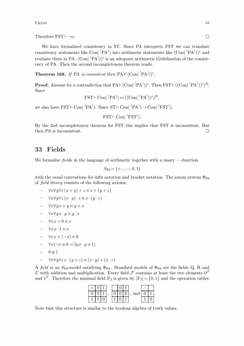
Therefore FST⊢¬α . �
We have formalized consistency in ST. Since PA interprets FST we can translate
consistency statements like Con( ⌈PA⌉) into arithmetic statements like (Con( ⌈PA⌉))ε and
evaluate them in PA. (Con( ⌈PA⌉))ε is an adequate arithmetic Gödelization of the consist-ency of PA. Then the second incompleteness theorem reads:
Theorem 168. If PA is consistent then PA� (Con( ⌈PA⌉))ε.
Proof. Assume for a contradiction that PA⊢ (Con( ⌈PA⌉))ε. Then FST⊢ ((Con( ⌈PA⌉))ε)N.Since
FST⊢Con( ⌈PA⌉)↔ ((Con( ⌈PA⌉))ε)N,
we also have FST⊢Con( ⌈PA⌉). Since ST⊢Con( ⌈PA⌉)→Con( ⌈FST⌉),
FST⊢Con( ⌈FST⌉).
By the 2nd incompleteness theorem for FST this implies that FST is inconsistent. Butthen PA is inconsistent. �
33 Fields
We formalize fields in the language of arithmetic together with a unary − -function
SFd= {+, ·,−, 0, 1}
with the usual conventions for infix notation and bracket notation. The axiom system ΦFd
of field theory consists of the following axioms:
− ∀x∀y∀z (x+ y)+ z≡ x+ (y+ z)
− ∀x∀y∀z (x · y) · z≡ x · (y · z)
− ∀x∀yx+ y≡ y+ x
− ∀x∀yx · y≡ y · x
− ∀xx+0≡x
− ∀xx · 1≡x
− ∀xx+(−x)≡ 0
− ∀x(¬x≡ 0→∃yx · y≡ 1)
− 0≡/ 1
− ∀x∀y∀z x · (y+ z)≡ (x · y)+ (x · z)
A field is an SFd-model satisfying ΦFd . Standard models of ΦFd are the fields Q, R andC with addition and multiplication. Every field F contains at least the two elements 0F
and 1F . Therefore the minimal field F2 is given by |F2|= {0, 1} and the operation tables
+ 0 1
0 0 11 1 0
,
· 0 1
0 0 01 0 1
, and
−
0 11 0
.
Note that this structure is similar to the boolean algebra of truth values.
Fields 83


![Programming - Research Institute for Mathematical Scienceskyodo/kokyuroku/contents/pdf/...logic programs, such as termination problem and total 243 correctness. [4], [5] To characterize](https://img.pdfslide.tips/doc/110x75/602f81567f59e2621578ce65/programming-research-institute-for-mathematical-kyodokokyurokucontentspdf.jpg)