Chapter 1

Mathematical Methods

In this chapter we will study basic mathematical methods for characterizing noise pro-cesses. The two important analytical methods, probability distribution functions andFourier analysis, are introduced here. These two methods will be used frequently through-out this text not only for classical systems but also for quantum systems. We try to presentthe two mathematical methods in a compact and succinct way as much as possible. Thereaders may find more detailed discussions in excellent texts [1]-[6]. In particular, mostof the discussions in this chapter follow the texts by M.J. Buckingham [1] and by A.W.Drake [2].

1.1 Time Average vs. Ensemble Average

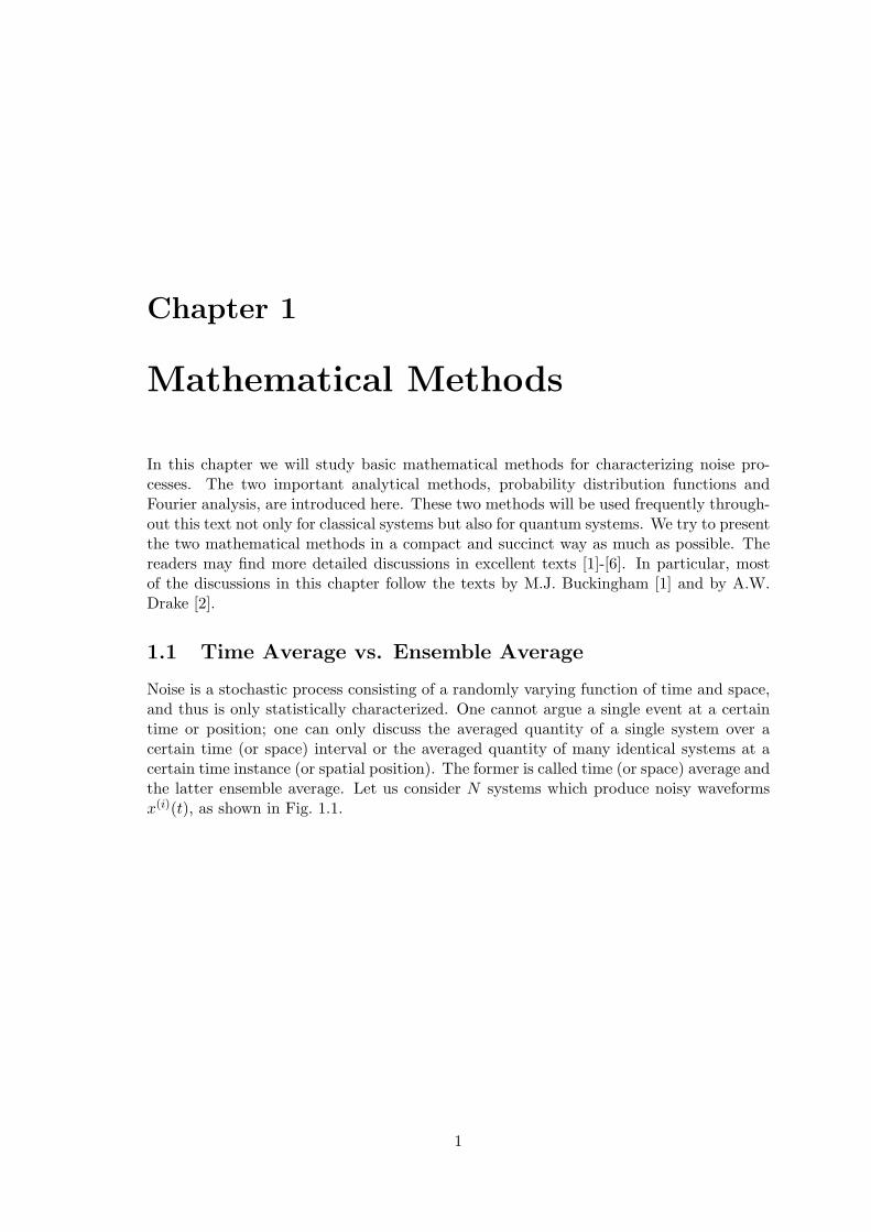
Noise is a stochastic process consisting of a randomly varying function of time and space,and thus is only statistically characterized. One cannot argue a single event at a certaintime or position; one can only discuss the averaged quantity of a single system over acertain time (or space) interval or the averaged quantity of many identical systems at acertain time instance (or spatial position). The former is called time (or space) average andthe latter ensemble average. Let us consider N systems which produce noisy waveformsx(i)(t), as shown in Fig. 1.1.

1

Figure 1.1: Ensemble average vs. time average.

One can define the following time-averaged quantities for the i-th member of the en-semble:

x(i)(t) = limT→∞

1T

∫ T2

−T2

x(i)(t)dt ,

(mean = first-order time average) (1.1)

x(i)(t)2 = limT→∞

1T

∫ T2

−T2

[x(i)(t)

]2dt ,

(mean square = second-order time average) (1.2)

φ(i)x (τ) ≡ x(i)(t)x(i)(t + τ) = lim

T→∞1T

∫ T2

−T2

x(i)(t)x(i)(t + τ)dt .

(autocorrelation function) (1.3)

One can also define the following ensemble-averaged quantities for all members of theensemble at a certain time:

〈x(t1)〉 = limN→∞

1N

N∑

i=1

x(i)(t1) =∫ ∞

−∞x1p1(x1, t1)dx1 ,

(mean = first-order ensemble average) (1.4)

〈x(t1)2〉 = limN→∞

1N

N∑

i=1

[x(i)(t1)

]2=

∫ ∞

−∞x2

1p1(x1, t1)dx1 ,

(mean square = second-order ensemble average) (1.5)

2

〈x(t1)x(t2)〉 = limN→∞

1N

N∑

i=1

x(i)(t1)x(i)(t2) (1.6)

=∫ ∞

−∞x1x2p2(x1, x2; t1, t2)dx1dx2 .

(covariance )

Here, x1 = x(t1), x2 = x(t2), p1(x1, t1) is the first-order probability density function(PDF), and p2(x1, x2; t1, t2) is the second-order joint probability density function.p1(x1, t1)dx1 is the probability that x is found in the range between x1 and x1 + dx1

at a time t1 and p2(x1, x2; t1, t2)dx1dx2 is the probability that x is found in the rangebetween x1 and x1 + dx1 at a time t1 and also in the range between x2 and x2 + dx2 at adifferent time t2.

An ensemble average is a convenient theoretical concept since it is directly relatedto the probability density functions, which can be generally obtained by the theoreticalanalysis of a given physical system. On the other hand, a time average is more directlyrelated to real experiments. One cannot prepare an infinite number of identical systemsin a real situation. Theoretical predictions based on ensemble averaging are equivalent toexperimental measurement results corresponding to time averaging when, and only when,the system is a so-called “ergodic ensemble.” It is often said that ensemble averaging andtime averaging are identical for a statistically-stationary system, but are different for astatistically-nonstationary system. We will see those concepts next and show there is asubtle difference between ergodicity and statistical stationarity.

1.2 Statistically Stationary vs. Nonstationary Processes

If 〈x(t1)〉 and 〈x(t1)2〉 are independent of the time t1 and if 〈x(t1)x(t2)〉 is independent ofabsolute times t1 and t2 but dependent only on the time difference τ = t2−t1, such a noiseprocess is called a “statistically-stationary” process. For a “statistically-nonstationary”process, the above is not true. In such a case, the concept of ensemble averaging is stillvalid, but the concept of time averaging fails.

The statistics of a stationary process do not change in time. To be more precise, wemake the following definitions. A stochastic process is stationary of order k if the k-thorder joint probability density function satisfies,

P (α1, . . . , αk; t1, . . . , tk) = P (α1, . . . , αk; t1 + ε, . . . , tk + ε) for all ε . (1.7)

Thus, if P1(x; t1) = P1(x; t1 + ε), the process is stationary of order 1. If P2(x1, x2; t1, t2) =P2(x1, x2; t1 + ε, t2 + ε), the process is stationary of order 2.

Since there are several types of stationarity, some special terminology has arisen. Aprocess is strictly stationary if it is stationary for any order, k = 1, 2, . . .. A process is calledwide-sense (or weakly) stationary if its mean value is constant and its autocorrelationfunction depends only on τ = t2 − t1. Wide-sense stationary processes can be analyzedby the Wiener-Khinchine theorem of Fourier transform, which we will discuss shortly. Ifa process is wide-sense stationary, the autocorrelation function and the power spectraldensity function form a Fourier transform pair. Therefore, if we know—or can measure—the autocorrelation function, we can find the power spectral density function, i.e. whichfrequencies contain how much power in the signal.

3

The idea of ergodicity arises if we have only one sample function of a stochastic process,instead of the entire ensemble. A single sample function will often provide little informationabout the statistics of the process. However, if the process is ergodic, that is, time averagesequal ensemble averages, then all statistical information can be derived from just onesample function.

When a process is ergodic, any one sample function represents the entire process. Alittle thought should convince you that the process must necessarily be stationary for thisto occur. Thus ergodicity implies stationarity. There are levels of ergodicity, just as thereare levels (degrees) of stationarity. We will discuss two levels of ergodicity; ergodicity inthe mean and correlation.

Level 1. A process is ergodic in the mean if

x(t) = limT→∞

1T

∫ T2

−T2

x(t)dt = 〈x(t)〉 (1.8)

We can compute the left-hand side of Eq. (1.8) by first selecting a particular memberfunction x(t) and then averaging in time. To compute the right-hand side, we must knowthe first-order PDF P1(x; t). The left-hand side of Eq. (1.8) is independent of t. Hencethe mean must be a constant value. Therefore, ergodicity of the mean implies stationarityof the mean. However, stationarity of the mean does not imply ergodicity of the mean, asour example below indicates.

4

Level 2. A process is ergodic in the autocorrelation if

φx(τ) = x(t)x(t + τ) = limT→∞

1T

∫ T2

−T2

x(t)x(t + τ)dt

= 〈x(t)x(t + τ)〉 (1.9)

We can compute the left-hand side of Eq. (1.9) by using a particular function x(t). Tocompute the right-hand side, we must know the second-order PDF P2(x1, x2; t1, t2).

EXAMPLE 1. Consider a basket full of batteries. There are some flashlight batteries,some car batteries, and several other kinds of batteries. Suppose that a battery is selectedat random and its voltage is measured. This battery voltage υ(t) is a member functionselected from a certain sub-group of constant battery voltages. This process is stationarybut not ergodic in the mean or correlation. The time average is equal to the particular bat-tery voltage selected (say, 1.5V). The statistical average is some other number, dependingon what is in the basket. Thus Eq. (1.8) does not hold.

EXAMPLE 2. Let x(t) = sin(ωt + θ) be a member function from a stochastic processspecified by a transformation of variables. Let θ be a random variable with uniformdistribution over the interval 0 < θ ≤ 2π.

P (θ) =12π

, 0 < θ ≤ 2π . (1.10)

Then each θ determines a time function x(t), which means that the stochastic process isspecified by a transformation of variables. This stochastic process is ergodic in both themean and autocorrelation. You can see that the time average of x(t) is 0. The ensembleaverage at any one time is over an infinite variety of sinusoids of all phases, and so mustalso be 0. Since the time average equals the ensemble average, the process is ergodic inthe mean. It is also true that Eq. (1.9) holds, so the process is ergodic in the correlation.For any other distribution of θ, the process is not stationary and hence not ergodic.

1.3 Basic Stochastic Processes

A noisy waveform x(t) often consists of a very large number of random and discrete pulses,and are represented by

x(t) =K∑

k=1

akf(t− tk) . (1.11)

One assumes the pulse amplitude ak and the time of pulse emission event tk are randomvariables, but the pulse-shape function f(t) is a fixed function, as shown in Fig. 1.2. Ina real physical situation, f(t) is often determined by an inherent property of a system,for example, by the relaxation time of a circuit or the transit time of a charged carrier.Therefore we assume here that f(t) is a fixed function.

Next let us consider the characteristics of several stochastic processes, which suchrandom variables ak and tk obey. It is convenient to use the probability density functionsand moment generating functions for this purpose.

5

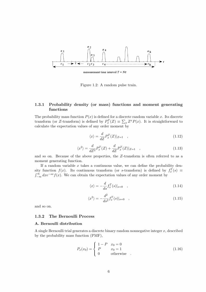
Figure 1.2: A random pulse train.

1.3.1 Probability density (or mass) functions and moment generatingfunctions

The probability mass function P (x) is defined for a discrete random variable x. Its discretetransform (or Z-transform) is defined by P T

x (Z) ≡ ∑x ZxP (x). It is straightforward to

calculate the expectation values of any order moment by

〈x〉 =d

dZP T

x (Z)|Z=1 , (1.12)

〈x2〉 =d

dZ2P T

x (Z) +d

dZP T

x (Z)|Z=1 , (1.13)

and so on. Because of the above properties, the Z-transform is often referred to as amoment generating function.

If a random variable x takes a continuous value, we can define the probability den-sity function f(x). Its continuous transform (or s-transform) is defined by fT

x (s) ≡∫∞−∞ dxe−sxf(x). We can obtain the expectation values of any order moment by

〈x〉 = − d

dsfT

x (s)|s=0 , (1.14)

〈x2〉 = − d2

ds2fT

x (s)|s=0 , (1.15)

and so on.

1.3.2 The Bernoulli Process

A. Bernoulli distribution

A single Bernoulli trial generates a discrete binary random nonnegative integer x, describedby the probability mass function (PMF),

Px(x0) =

1− P x0 = 0P x0 = 10 otherwise .

(1.16)

6

Random variable x, described above, is known as a Bernoulli random variable. We definethe z transform (or discrete transform) of the PMF as,

PxT (z) ≡

∞∑

x0=0

zx0Px(x0) = z0(1− P ) + zP = 1− P + zP . (1.17)

It is easily understood by the definition of the PMF and Z transform that the mean andmean-square are given by

〈x〉 =[

d

dzP T

x (z)]

z=1=

∑x0

x0Px(x0) , (1.18)

〈x2〉 =

[d2

dz2P T

x (z) +d

dzP T

x (z)

]

z=1

=∑x0

x20Px(x0) . (1.19)

By use of these relations and (1.17), we find the mean, mean-square and variance of theBernoulli process:

〈x〉 = p, 〈x2〉 = p, σx2 ≡ 〈x2〉 − 〈x〉2 = p(1− p) . (1.20)

We refer to the outcome of a Bernoulli trial as a pulse emission when the experimentalvalue of x is unity and as no emission when the experimental value of x is zero.

B. Binomial distribution

A Binomial distribution is obtained by a series of independent Bernoulli trials, each withthe same probability of success. Suppose that n independent Bernoulli trials are to beperformed, and define discrete random veriable k to be the number of successes in then trials. Note that random variable k is the sum of n independent Bernoulli randomvariables, i.e. k = x1 +x2 · · ·+xn, so the z transform of the PMF for the Bernoulli processis

P Tk (z)

∑x1···xn

Zx1···xnPx(x1) · · ·Px(xn) = [P Tx (z)]n = (1− p + zp)n (1.21)

= P Tx1

(Z) · · ·P Tx1

(Z)

There are several ways to determine Pk(k0), the probability of exactly k0 successes outof n independent Bernoulli trials. One way would be to apply the binomial theorem,

(a + b)n =n∑

l=0

(nl

)albn−l , (1.22)

to expand P Tk (z) in a power series,

P Tk (z) =

n∑

l=0

(nl

)(zP )l(1− P )n−l ,

and then compare the coefficients of zk0 in the expansion for the definition of the z trans-form (1.17),

P Tk (z) =

n∑

k0=0

zk0Pk(k0) = Pk(0) + zPk(1) + z2Pk(2) + · · · .

7

This leads to the result known as the binomial PMF,

Pk(k0) =

(nk0

)pk0(1− p)n−k0 , k0 = 0, 1, 2, . . . ,n , (1.23)

where (nk0

)=

n!(n− k0)!k0!

,

as commonly used.We can determine the expected value and variance of the binomial random variable k

by any of the following three techniques. To evaluate 〈k〉 and σk2 we may

1. perform the expected value summations directly,

2. use the moment-generating properties (1.18) and (1.19) of the z transform, or

3. recall that the expected value of a sum of random variables is always equal to thesum of their expected values and that the variance of a sum of linearly independentrandom variables is equal to the sum of their individual variances.

Since we know that a binomial random variable k is the sum of n independent Bernoullirandom variables, the last of the above methods is the easiest and we obtain

〈k〉 = n〈x〉 = np , σk2 = nσx

2 = np(1− p) . (1.24)

C. Geometric distribution

It is often convenient to refer to the successes in a Bernoulli process as pulse emission. Leta discrete random variable l1 be the number of Bernoulli trials after any pulse emissionand before the next pulse emission, including this pulse emission. The random variable l1is known as the first-order interarrival time of pulses, and it can take on the experimentalvalues 1, 2, . . .. We begin by determining the PMF Pl1(l).

We shall determine Pl1(l) from a sequential sample space for the experiment of per-forming independent Bernoulli trials until we obtain our first success. Using the notationof the last section, we have

Pl1(l) = p(1− p)l−1 l = 1, 2, . . . , (1.25)

and since its successive terms decrease in a geometric progression, this PMF for the first-order interarrival times is known as the geometric PMF. The z transform for the geometricPMF is

Pl1T (z) =

∞∑

l=1

Pl1(l)zl =

∞∑

l=1

p(1− p)l−1zl =zp

1− z(1− p). (1.26)

Since direct calculation of 〈l1〉 and σl12 in an l1 event space involves difficult summa-

tions, we shall use the moment-generating property of the z transform to evaluate thesequantities.

〈l1〉 =[

d

dzPl1

T (z)]

z=1=

1p

, (1.27)

σl12 =

{d2

dz2Pl1

T (z) +d

dzPl1

T (z)−[

d

dzPl1

T (z)]2

}

z=1

=1− p

p2. (1.28)

8

1.3.3 The Poisson Process

A. Poisson distribution

We defined the Bernoulli process by a particular probabilistic description of the “arrivals”of successes in a series of independent identical discrete trials. A Poisson process will bedefined by a probabilistic description of the behavior of arrivals of successes at points ona continuous line.

For convenience, we shall generally refer to this line as a time (t) axis. By definitionof the process, we shall see that a Poisson process may be considered to be in the limitof ∆t → 0 of a series of identical independent Bernoulli trials at intervals of ∆t, with theprobability of a success, p = λ∆t.

For our study of the Poisson process we shall adopt the probability that there areexactly k arrivals during any interval of duration t, ℘(k, t). This notation is compact andparticularly convenient for the types of equations to follow. We observe that ℘(k, t) is aPMF for a random variable k for any fixed value of parameter t. In any interval of lengtht, with t ≥ 0, we must have exactly zero, or exactly one, or exactly two, etc., arrivals ofsuccesses. Thus we have ∞∑

k=0

℘(k, t) = 1 . (1.29)

We also note that ℘(k, t) is not a probability density function (PDF) for t. Since ℘(k, t1)and ℘(k, t2) are not mutually exclusive events, we can state only that

0 ≤∫ ∞

0℘(k, t) dt < ∞ . (1.30)

The use of a random variable k to count arrivals is consistent with our notation for countingsuccesses in a Bernoulli process.

There are several equivalent ways to define a Poisson process. We shall define it directlyin terms of those properties which are most useful for the analysis of problems based onphysical situations.

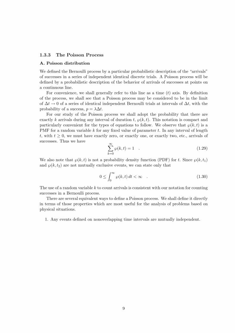
1. Any events defined on nonoverlapping time intervals are mutually independent.

9

2. The following statements are correct in the limit of ∆t → 0:

℘(k, ∆t) =

1− λ∆t k = 0λ∆t k = 10 k > 1

. (1.31)

The first of the above two defining properties establishes the no-memory attribute ofthe Poisson process. The second defining property of the Poisson process states that, forsmall intervals, the probability of having exactly one arrival within one such interval isproportional to the duration of the interval and that, to the first order, the probability ofmore than one arrival within one such interval is zero. This simply means that ℘(k, ∆t)can be expanded in a Taylor series about ∆t = 0, and when we neglect terms of order(∆t)2 or higher, we obtain the given expressions for ℘(k, ∆t).

We wish to determine the expression for ℘(k, t) for t ≥ 0 and for k=0, 1, 2, . . .. Beforedoing mathematical derivation, let us reason out how we would expect the result to behave.By definition of the Poisson process and our interpretation of it as a series of Bernoullitrials in incremental intervals, we expect that

1. ℘(0, t) as a function of t will be unity at t=0 and decrease monotonically toward zeroas t increases. (The event of exactly zero arrivals in an interval of length t requiresmore and more successive failures in incremental intervals as t increases.)

2. ℘(k, t) as a function of t, for k > 0, should start out at zero for t=0, increase for awhile, and then decrease toward zero as t gets very large. [The probability of havingexactly k arrivals (with k > 0) should be very small for intervals which are too longor too short.]

For a Poisson process, if ∆t is small enough, we need to consider only the possibilityof zero or one arrivals between t and t + ∆t. Taking advantage also of the independenceof events in nonoverlapping time intervals, we may write

℘(k, t + ∆t) = ℘(k, t)℘(0, ∆t) + ℘(k − 1, t)℘(1,∆t) . (1.32)

The two terms summed on the right-hand side are the probabilities of the only two (mu-tually exclusive) histories of the process which may lead to having exactly k arrivals in aninterval of duration t + ∆t. Our definition of (1.31) for the process specified ℘(0,∆t) and℘(1, ∆t) for a small ∆t. We substitute for these quantities to obtain,

℘(k, t + ∆t) = ℘(k, t)(1− λ∆t) + ℘(k − 1, t)λ∆t . (1.33)

Collecting terms, dividing through by ∆t, and taking the limit of ∆t → 0, we find

d

dt℘(k, t) + λ℘(k, t) = λ℘(k − 1, t) . (1.34)

This may be solved iteratively for k = 0 and then for k = 1, and so on, with the initialconditions,

℘(k, 0) =

{1 k = 00 k 6= 0

. (1.35)

10

The solution for ℘(k, t), which may be verified by direct substitution, is

℘(k, t) =(λt)ke−λt

k!t ≥ 0, k = 1, 2, . . . . (1.36)

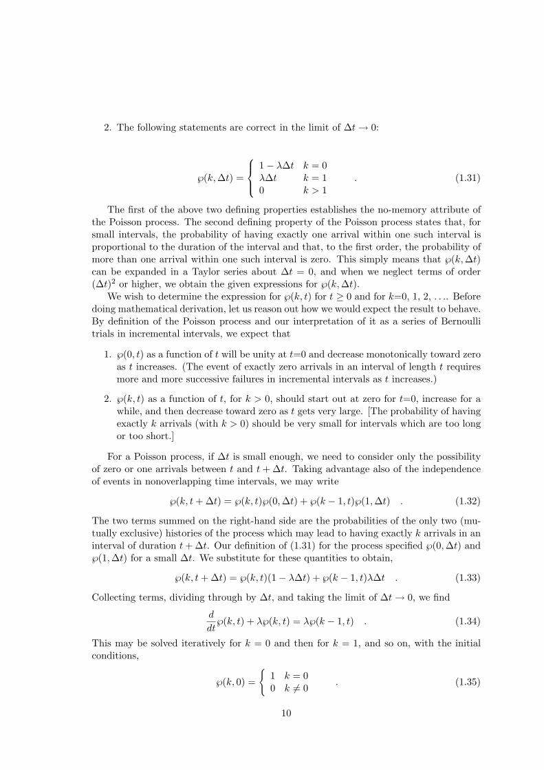
We find that ℘(k, t) does have the properties we anticipated earlier, as shown in Fig. 1.3.

Figure 1.3: P(k, t) in a Poisson process.

Letting µ = λt, we may write this result in the more proper notation for a PMF as

Pk(k0) =µk0e−µ

k0!µ = λt, k0 = 0, 1, 2, . . . . (1.37)

This is known as the Poisson PMF. Although we derived the Poisson PMF by consideringthe number of arrivals in an interval of length t for a certain process, this PMF arisesfrequently in many other situations.

To obtain the mean value and variance of the Poisson PMF, we will use the z transform,

PkT (z) =

∞∑

k0=0

Pk(k0)zk0 = e−µ∞∑

k0=0

(µz)k0

k0!= eµ(z−1) , (1.38)

〈k〉 =[

d

dzPk

T (z)]

z=1= µ , (1.39)

σk2 =

{d2

dz2Pk

T (z) +d

dzPk

T (z)−[

d

dzPk

T (z)]2

}

z=1

= µ . (1.40)

Thus the mean value and variance of Poisson random variable k are both equal to µ.We may also note that, since 〈k〉 = λt, we have an interpretation of the constant λ

used in

℘(k, ∆t) =

1− λ∆t k = 0λ∆t k = 10 k = 2, 3, . . .

. (1.41)

as part of the definition of the Poisson process. The relation 〈k〉 = λt indicates that λis the expected number of arrivals per unit time in a Poisson process. The constant λ isreferred to as the average arrival rate for the process.

11

B. Erlang distribution

Let lr be a continuous random variable defined to be an interval of time between anyarrivals in a Poisson process and the r-th arrival after that. The continuous randomvariable lr, the r-th order interarrival time, has the same interpretation here as the discreterandom variable lr had for the Bernoulli process.

We wish to determine the PDF’s

flr(l) l ≥ 0; r = 1, 2, 3, . . .

For a small ∆l we may write

Prob(l < lr ≤ l + ∆l) = flr(l)∆l , (1.42)

flr(l)∆l = ℘(r − 1, l)︸ ︷︷ ︸A

λ∆l︸︷︷︸B

=(λl)r−1e−λl

(r − 1)!λ∆l l ≥ 0; r = 1, 2, . . . , (1.43)

where

A = probability that there are exactly r − 1 arrivals in an interval of duration l

B = conditional probability that rth arrival occurs in next ∆l, given exactly r−1 arrivalsin previous interval of duration l

Thus we have obtained the PDF for the rth-order interarrival time

flr(l) =λrlr−1e−λl

(r − 1)!l ≥ 0; r = 1, 2, . . . , (1.44)

which is known as the Erlang family of PDF’s. Random variable lr is said to be an Erlangrandom variable of order r.

The first-order interarrival time, described by random variable l1, has the PDF

fl1(l) = λe−λl (1.45)

which is the exponential PDF. We may obtain its mean and variance by use of the stransform:

fl1T (s) =

∫ ∞

−∞e−slfl1(l)dl =

λ

s + λ, (1.46)

〈l1〉 = −[

d

dsfl1

T (s)]

s=0=

1λ

, (1.47)

σl12 =

{d2

ds2fl1

T (s)−[

d

dsfl1

T (s)]2

}

s=0

=1λ2

. (1.48)

The random variable lr is the sum of r independent experimental values of randomvariable l1. Therefore we have

flrT (s) =

∫dl1 · · ·

∫dlre

−s(l1+···+lr)fl1(l) · · · flr(l)

= fTl1 (s) · · · fT

lr (s)

=[fl1

T (s)]r

=(

λ

s + λ

)r

,

〈lr〉 = r〈l1〉 =r

λ, σlr

2 = rσl12 =

r

λ2.

12

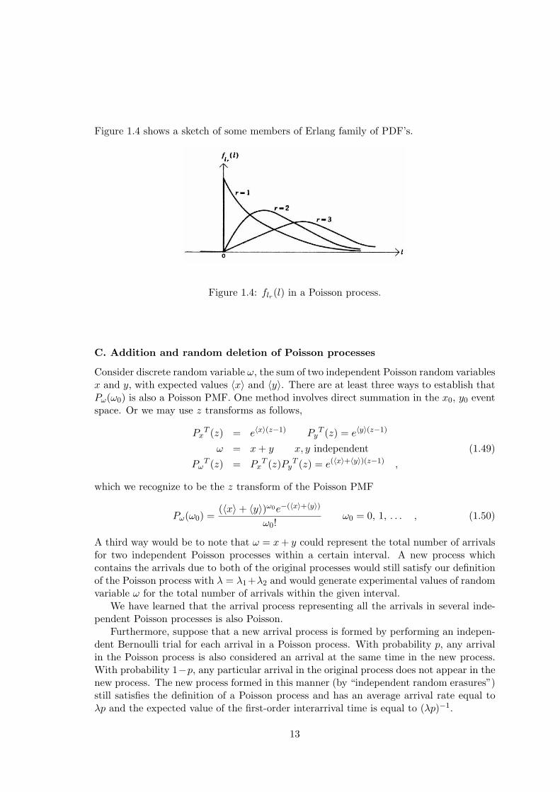
Figure 1.4 shows a sketch of some members of Erlang family of PDF’s.

Figure 1.4: flr(l) in a Poisson process.

C. Addition and random deletion of Poisson processes

Consider discrete random variable ω, the sum of two independent Poisson random variablesx and y, with expected values 〈x〉 and 〈y〉. There are at least three ways to establish thatPω(ω0) is also a Poisson PMF. One method involves direct summation in the x0, y0 eventspace. Or we may use z transforms as follows,

PxT (z) = e〈x〉(z−1) Py

T (z) = e〈y〉(z−1)

ω = x + y x, y independent (1.49)Pω

T (z) = PxT (z)Py

T (z) = e(〈x〉+〈y〉)(z−1) ,

which we recognize to be the z transform of the Poisson PMF

Pω(ω0) =(〈x〉+ 〈y〉)ω0e−(〈x〉+〈y〉)

ω0!ω0 = 0, 1, . . . , (1.50)

A third way would be to note that ω = x + y could represent the total number of arrivalsfor two independent Poisson processes within a certain interval. A new process whichcontains the arrivals due to both of the original processes would still satisfy our definitionof the Poisson process with λ = λ1+λ2 and would generate experimental values of randomvariable ω for the total number of arrivals within the given interval.

We have learned that the arrival process representing all the arrivals in several inde-pendent Poisson processes is also Poisson.

Furthermore, suppose that a new arrival process is formed by performing an indepen-dent Bernoulli trial for each arrival in a Poisson process. With probability p, any arrivalin the Poisson process is also considered an arrival at the same time in the new process.With probability 1−p, any particular arrival in the original process does not appear in thenew process. The new process formed in this manner (by “independent random erasures”)still satisfies the definition of a Poisson process and has an average arrival rate equal toλp and the expected value of the first-order interarrival time is equal to (λp)−1.

13

If the erasures are not independent, then the derived process has memory. For instance,if we erase alternate arrivals in a Poisson process, the remaining arrivals do not form aPoisson process. It is clear that the resulting process violates the definition of the Poissonprocess, since, given that an arrival in the new process just occurred, the probability ofanother arrival in the new process in the next ∆t is zero (this would require two arrivals in∆t in the underlying Poisson process). This particular derived process is called an Erlangprocess since the first-order interarrival times are independent and have (second-order)Erland PDF’s. This derived process is one example of how we can use the memorylessPoisson process to model more complicated situations with memory.

1.3.4 The Gaussian Process

A. Gaussian PDF

When the total number of trials n is very large and both the success and failure probabili-ties p and 1−p are not very close to zero, the binomial distribution (1.23) tends to exhibita pronounced maximum at some value k0 = k̃0, and to decrease rapidly as one goes awayfrom k̃0. If n is large and we consider regions near the maximum of Pk(k0) where k0 isalso large, the fractional change in Pk(k0) when k0 changes by unity is relatively small,i.e.

|Pk(k0 + 1)− Pk(k0)| ¿ Pk(k0) . (1.51)

Thus Pk(k0) can, to good approximation, be considered as a continuous function of thevariable k0, although only integral values of k0 are of physical relevance. The locationk0 = k̃0 of the maximum of Pk is then approximately determined by the condition

dPk

dk0= 0 or

d lnPk

dk0= 0 , (1.52)

where the derivatives are evaluated at k0 = k̃0. To evaluate the behavior of Pk(k0) nearits maximum, we shall put

k0 = k̃0 + η , (1.53)

and expand lnPk(k0) in a Taylor’s series about k̃0. The reason for expanding lnPk, ratherthan Pk itself, is that lnPk is a much more slowly varying function of k0 than Pk. Thusthe power series expansion for lnPk should converge much more rapidly than the one forPk.

Expanding lnPk in Taylor’s series, we obtain

ln Pk(k0) = lnPk(k̃0) + B1η +12B2η

2 +16B3η

3 + · · · , (1.54)

where

Bl =dl ln Pk

dk0l

, (1.55)

is the l-th derivative of lnPk evaluated at k̃0. Since we are expanding about a maximum,B1 = 0 by (1.52). Since Pk is a maximum, the term 1

2B2η2 must be negative. Let us write

B2 = −|B2|, and we obtain

Pk(k0) = P̃ke− 1

2|B2|η2

e16B3η3 · · · . (1.56)

14

In the region where η is sufficiently small, higher-order terms in the expansion can beneglected, i.e. B3 = · · · · · · = 0. By the binomial distribution (1.23), we obtain

lnPk(k0) = lnn!− ln k0!− ln(n− k0)! + k0 ln p + (n− k0) ln(1− p) . (1.57)

If n is any large integer so that n À 1, then ln n! can be considered an almost continuousfunction of n, since ln n! changes only by a small fraction of itself if n is changed by asmall integer. Here

d

dnln n! ' ln (n + 1)!− ln n!

(n + 1)− n= ln (n + 1)

' ln n . (1.58)

Thus Eq. (1.57) yields

d

dk0ln Pk = − ln k0 + ln (n− k0) + ln p− ln(1− p) . (1.59)

By equating this first derivative to zero, we find an expected result

k̃0 = np . (1.60)

Further differentiation of (1.59) yields

d2

dk02 lnPk = − 1

k0− 1

n− k0. (1.61)

Evaluating this for the value k0 = k̃0 given in (1.61), we get

B2 = − 1np(1− p)

. (1.62)

The value of the constant P̃k in (1.56) can be determined from the normalizationcondition

∑∞k0=1 Pk(k0) = 1. Since Pk and k0 can be considered as continuous variables,

the sum over all integral values of k0 can be approximately replaced by an integral. Thusthe normalization condition can be written

∫ ∞

−∞Pk(k0)dk0 = P̃k

∫ ∞

−∞e−

12|B2|η2

dη = P̃k

√2π

|B2| = 1 . (1.63)

The final expression for Pk(k0) is thus given by

Pk(k0) =1√

2πσ2k0

exp

[−(k0 − k̃0)2

2σ2k0

], (1.64)

whereσ2

k0= np(1− p) . (1.65)

This is the so-called Gaussian distribution. The Gaussian distribution is very general innature and occur very frequently in statistical mechanics whenever we are dealing withlarge numbers of particles.

15

B. Gaussian s-transform

The s-transform of the Gaussian PDF (1.64) is written as

fTk0

(s) =∫ ∞

−∞dk0e

−sk0pk(k0) (1.66)

= e−sk̃0+ 1

2s2σ2

k0 .

Using the moment generating properties (1.18) and (1.19), we find the mean and varianceare identical to k̃0 and σ2

k0as expected.

1.4 Burgess Variance Theorem

In the discussion of the Bernoulli process, we start with a fixed (constant) number of trialsn and introduce random deletion with the probability 1− p. The variance of the outputevent (1.24) is a rather general result for such a stochastic process and the fluctuationassociated with such random deletion is referred to as “partition noise.” In some cases,the total number of trials n itself fluctuates. In such a case, the probability of obtainingk0 successes is given by

P (k0) =∞∑

n=k0

W (n)Pk(k0) , (1.67)

where W (n) is the distribution (PMF) of the total number of trials and Pk(k0) is thebinomial distribution of obtaining k0 successes out of n trials. The mean and mean-squareof k0 can be evaluated by using (1.24) and (1.67),

〈k0〉 ≡∞∑

k0=0

k0P (k0) =∞∑

n=0

n∑

k0=0

k0Pk(k0)W (n)

=∞∑

n=0

pnW (n)

= p〈n〉 , (1.68)

〈k02〉 ≡

∞∑

k0=0

k02P (k0) =

∞∑

n=0

n∑

k0=0

k02Pk(k0)W (n)

=∞∑

n=0

[(pn)2 + p(1− p)n

]W (n)

= p2〈n2〉+ p(1− p)〈n〉 . (1.69)

The variance of the number of successful events is given by

σ2k0

= 〈k20〉 − 〈k0〉2 = σ2

np2 + 〈n〉p(1− p) , (1.70)

where σ2n = 〈n2〉 − 〈n〉2. The above relation is known as the “Burgess variance theorem”.

The first term on the right-hand side of (1.70) indicates that the fluctuation of the initialnumber of trials is suppressed by a “loss” probability p2. The second term, on the other

16

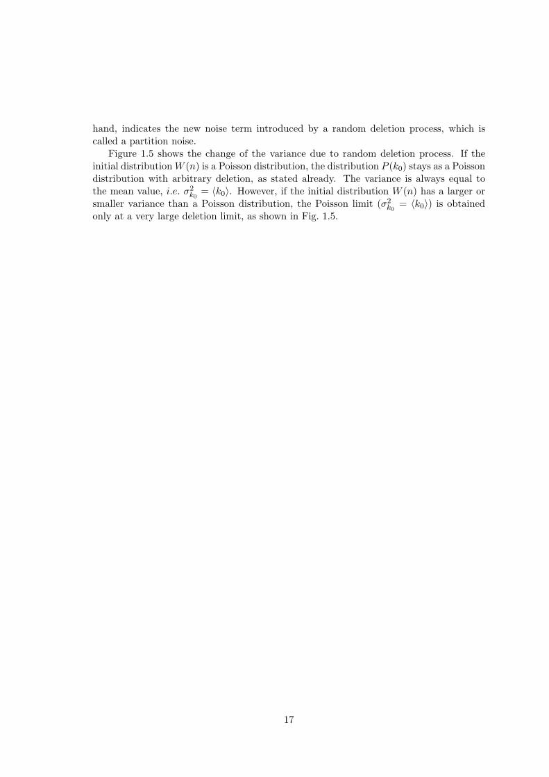
hand, indicates the new noise term introduced by a random deletion process, which iscalled a partition noise.

Figure 1.5 shows the change of the variance due to random deletion process. If theinitial distribution W (n) is a Poisson distribution, the distribution P (k0) stays as a Poissondistribution with arbitrary deletion, as stated already. The variance is always equal tothe mean value, i.e. σ2

k0= 〈k0〉. However, if the initial distribution W (n) has a larger or

smaller variance than a Poisson distribution, the Poisson limit (σ2k0

= 〈k0〉) is obtainedonly at a very large deletion limit, as shown in Fig. 1.5.

17

Figure 1.5: The change of the variance for a Poisson (σ2N = N), super-Poisson

(σ2N = 2N) and sub-Poisson (σ2

N = 12N) distributions due to a partition pro-

cess.

18

1.5 Fourier Analysis

When x(t) is absolutely integrable, i.e.,∫ ∞

−∞|x(t)|dt < ∞ , (1.71)

the Fourier transform of x(t) exists and is defined by

X(iω) =∫ ∞

−∞x(t)e−iωtdt . (1.72)

The inverse transform is given by

x(t) =12π

∫ ∞

−∞X(iω)eiωtdω . (1.73)

This inverse relation is proven by substituting for X(iω) from (1.72), and interchangingthe order of integration to obtain

12π

∫ ∞

−∞X(iω)eiωtdω =

12π

∫ ∞

−∞dωeiωt

∫ ∞

−∞x(t′)e−iωt′dt′

=∫ ∞

−∞x(t

′)δ(t

′ − t)dt′

= x(t) , (1.74)

where we use12π

∫ ∞

−∞dωeiω(t−t′) = δ(t′ − t) .

When x(t) is a real function of time, as it always is the case for an “observable” waveform,the real part of X(iω) is an even function of ω and the imaginary part is an odd functionof ω [i.e., X(iω) = X∗(−iω)].

When x(t) is a statistically-stationary process, condition (1.71) is not satisfied andthus the Fourier transform cannot be defined. The total energy of the noisy waveformx(t) is infinite, but in any practical noise measurement, a measurement time interval T isfinite and the energy of such a gated function xT (t), defined by

xT (t) =

x(t) |t| ≤ T2

0 |t| > T2

, (1.75)

is also finite. The Fourier transform of such a gated function “does” exist.

1.5.1 Parseval theorem

If x1(t) and x2(t) have Fourier transforms X1(iω) and X2(iω), one obtains∫ ∞

−∞x1(t)x∗2(t)dt =

∫ ∞

−∞dtx1(t)

12π

∫ ∞

−∞dωX2(iω)∗e−iωt

=12π

∫ ∞

−∞dωX2(iω)∗

∫ ∞

−∞dtx1(t)e−iωt

=12π

∫ ∞

−∞X1(iω)X∗

2 (iω)dω . (1.76)

19

This relation is known as the Parseval theorem. If one uses x1(t) = xT (t + τ) and x2(t) =xT (t) in (1.76), one obtains

∫ ∞

−∞xT (t + τ)xT (t)dt =

12π

∫ ∞

−∞|XT (iω)|2eiωτdω , (1.77)

where∫∞−∞ xT (t + τ)e−iωtdt = XT (iω)eiωτ is used. When τ = 0, (1.77) is reduced to

∫ ∞

−∞[xT (t)]2dt =

12π

∫ ∞

−∞|XT (iω)|2dω . (1.78)

The physical interpretation of XT (iω) and |XT (iω)|2 is now clear from the above relations.XT (iω) is the (complex) amplitude of the harmonic (eiωt) component in a gated functionxT (t) and |XT (iω)|2 is the energy density of this harmonic component with units of energyper Hz. Equation (1.78) is the total energy of xT (t) and increases linearly with T for astatistically-stationary process.

1.5.2 Power spectral density and Wiener-Khintchine theorem

The average power of xT (t), defined by

limT→∞

1T

∫ ∞

−∞[xT (t)]2dt = lim

T→∞12π

∫ ∞

0

2|XT (iω)|2T

dω , (1.79)

is independent of T and a constant universal quantity, if x(t) is a statistically stationaryprocess. However, if x(t) is a statistically nonstationary process, the average power isdependent of T and we are not allowed to take the limit of T →∞. If ensemble averagingis taken first for many identical gated functions xT (t) in (1.79), the order of limT→∞ and∫∞0 dω can be interchanged. In this way, the power spectral density is defined as

Sx(ω) = limT→∞

2〈|XT (iω)|2〉T

.

(unilateral power spectral density) (1.80)

Note that the power spectral density is an ensemble averaged quantity and has the differentform for a stationary and nonstationary process.

When τ 6= 0 in (1.77), one can also divide both sides of (1.77) by T , take an ensembleaverage, and take a limit of T →∞ to obtain,

limT→∞

1T

∫ ∞

−∞〈xT (t + τ)xT (t)〉dt = lim

T→∞12π

∫ ∞

0

2〈|X(iω)|2〉T

cos ωτ dω . (1.81)

The left-hand side of this expression is the ensemble averaged autocorrelation functionφx(τ). Using (1.80) in the right-hand side of this expression, one obtains

φx(τ) =12π

∫ ∞

0Sx(ω) cos ωτ dω . (1.82)

The inverse relation of this expression is

4∫ ∞

0φx(τ) cos ωτ dτ =

2π

∫ ∞

0dω′Sx(ω′)

∫ ∞

0dτcos(ωτ)cos(ω′τ)

=∫ ∞

0dω′Sx(ω′)[δ(ω + ω′) + δ(ω − ω′)]

= Sx(ω) . (1.83)

20

Here we use the relation,∫ ∞

0dτcos(ωτ)cos(ω′τ) =

π

2[δ(ω + ω′) + δ(ω − ω′)] . (1.84)

Equations (1.82) and (1.83) constitute the Wiener-Khintchine theorem and indicate that2φx(τ) and Sx(ω) are the Fourier transform pairs.

If a noisy waveform x(t) is a nonstationary process, we cannot take a limit as T →∞in (1.81). The Wiener-Khintchine theorem for such a case is given by

φx(τ, T ) =12π

∫ ∞

0Sx(ω, T )cos(ωτ)dω , (1.85)

Sx(ω, T ) = 4∫ T

0φx(τ, T )cos(ωτ)dτ . (1.86)

1.5.3 Examples

Let us consider a few examples for demonstrating how to use the Wiener-Khintchinetheorem.

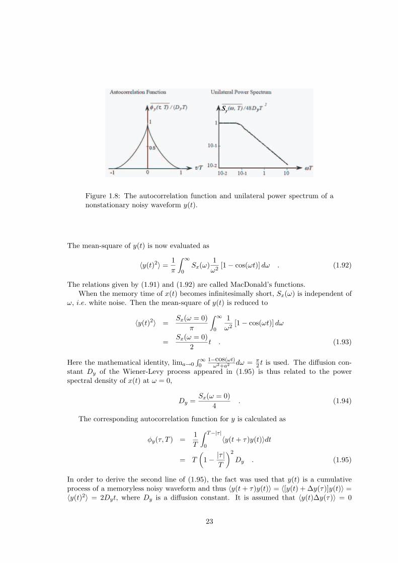
EXAMPLE 1. Suppose a noisy waveform x(t) is a statistically-stationary process, asshown in Fig. 1.6, with an exponentially decaying autocorrelation function

φx(τ) = φx(0) exp(−|τ |

τ1

), (1.87)

where φx(0) = 〈x2〉 by definition and τ1 is a relaxation time constant which is a system’smemory time. Substituting (1.87) into (1.83), one obtains the unilateral power spectraldensity

Sx(ω) =4φx(0)τ1

1 + ω2τ21

. (1.88)

The spectrum is Lorentzian with a cut-off frequency of ωc = 1/τ1 and the low-frequencyspectral density is Sx(ω = 0) = 4φx(0)τ1. The autocorrelation function and the unilateralpower spectrum are shown in Fig. 1.7.

EXAMPLE 2. A time-integrated function y(t) =∫ t0 x(t′) dt′ of a statistically-stationary

process x(t′) goes through a random walk diffusion, as shown in Fig. 1.6. If x(t) has aninfinitesimally short correlation time, τ1 → 0, its time-integrated waveform y(t) is called aWiener-Levy process and is a classic example of a statistically-nonstationary process. Letus define a gated function by

y(t) =

{ ∫ t0 x(t′) dt′ (0 ≤ t ≤ T )

0 (otherwise). (1.89)

If x(t) is a stationary noisy waveform with a finite memory time, we first have toevaluate the covariance function,

〈y(t)y(t + τ)〉 =∫ t

0

∫ t+τ

0〈x(t′)x(t′′)〉dt′dt′′ , (1.90)

21

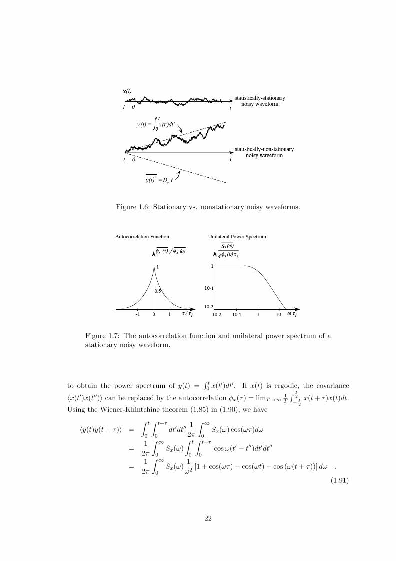
Figure 1.6: Stationary vs. nonstationary noisy waveforms.

Figure 1.7: The autocorrelation function and unilateral power spectrum of astationary noisy waveform.

to obtain the power spectrum of y(t) =∫ t0 x(t′)dt′. If x(t) is ergodic, the covariance

〈x(t′)x(t′′)〉 can be replaced by the autocorrelation φx(τ) = limT→∞ 1T

∫ T2

−T2

x(t + τ)x(t)dt.

Using the Wiener-Khintchine theorem (1.85) in (1.90), we have

〈y(t)y(t + τ)〉 =∫ t

0

∫ t+τ

0dt′dt′′

12π

∫ ∞

0Sx(ω) cos(ωτ)dω

=12π

∫ ∞

0Sx(ω)

∫ t

0

∫ t+τ

0cosω(t′ − t′′)dt′dt′′

=12π

∫ ∞

0Sx(ω)

1ω2

[1 + cos(ωτ)− cos(ωt)− cos (ω(t + τ))] dω .

(1.91)

22

Sy

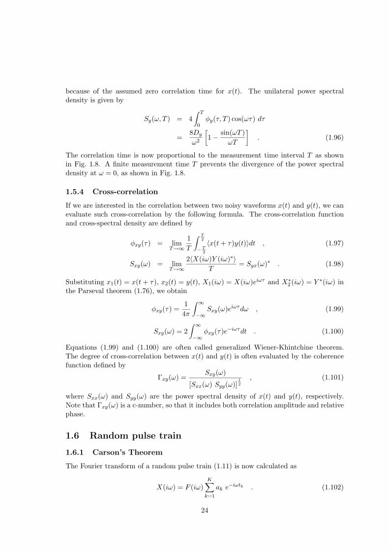
Figure 1.8: The autocorrelation function and unilateral power spectrum of anonstationary noisy waveform y(t).

The mean-square of y(t) is now evaluated as

〈y(t)2〉 =1π

∫ ∞

0Sx(ω)

1ω2

[1− cos(ωt)] dω . (1.92)

The relations given by (1.91) and (1.92) are called MacDonald’s functions.When the memory time of x(t) becomes infinitesimally short, Sx(ω) is independent of

ω, i.e. white noise. Then the mean-square of y(t) is reduced to

〈y(t)2〉 =Sx(ω = 0)

π

∫ ∞

0

1ω2

[1− cos(ωt)] dω

=Sx(ω = 0)

2t . (1.93)

Here the mathematical identity, lima→0∫∞0

1−cos(ωt)ω2+a2 dω = π

2 t is used. The diffusion con-stant Dy of the Wiener-Levy process appeared in (1.95) is thus related to the powerspectral density of x(t) at ω = 0,

Dy =Sx(ω = 0)

4. (1.94)

The corresponding autocorrelation function for y is calculated as

φy(τ, T ) =1T

∫ T−|τ |

0〈y(t + τ)y(t)〉dt

= T

(1− |τ |

T

)2

Dy . (1.95)

In order to derive the second line of (1.95), the fact was used that y(t) is a cumulativeprocess of a memoryless noisy waveform and thus 〈y(t + τ)y(t)〉 = 〈[y(t) + ∆y(τ)]y(t)〉 =〈y(t)2〉 = 2Dyt, where Dy is a diffusion constant. It is assumed that 〈y(t)∆y(τ)〉 = 0

23

because of the assumed zero correlation time for x(t). The unilateral power spectraldensity is given by

Sy(ω, T ) = 4∫ T

0φy(τ, T ) cos(ωτ) dτ

=8Dy

ω2

[1− sin(ωT )

ωT

]. (1.96)

The correlation time is now proportional to the measurement time interval T as shownin Fig. 1.8. A finite measurement time T prevents the divergence of the power spectraldensity at ω = 0, as shown in Fig. 1.8.

1.5.4 Cross-correlation

If we are interested in the correlation between two noisy waveforms x(t) and y(t), we canevaluate such cross-correlation by the following formula. The cross-correlation functionand cross-spectral density are defined by

φxy(τ) = limT→∞

1T

∫ T2

−T2

〈x(t + τ)y(t)〉dt , (1.97)

Sxy(ω) = limT→∞

2〈X(iω)Y (iω)∗〉T

= Syx(ω)∗ . (1.98)

Substituting x1(t) = x(t + τ), x2(t) = y(t), X1(iω) = X(iω)eiωτ and X∗2 (iω) = Y ∗(iω) in

the Parseval theorem (1.76), we obtain

φxy(τ) =14π

∫ ∞

−∞Sxy(ω)eiωτdω , (1.99)

Sxy(ω) = 2∫ ∞

−∞φxy(τ)e−iωτdt . (1.100)

Equations (1.99) and (1.100) are often called generalized Wiener-Khintchine theorem.The degree of cross-correlation between x(t) and y(t) is often evaluated by the coherencefunction defined by

Γxy(ω) =Sxy(ω)

[Sxx(ω) Syy(ω)]12

, (1.101)

where Sxx(ω) and Syy(ω) are the power spectral density of x(t) and y(t), respectively.Note that Γxy(ω) is a c-number, so that it includes both correlation amplitude and relativephase.

1.6 Random pulse train

1.6.1 Carson’s Theorem

The Fourier transform of a random pulse train (1.11) is now calculated as

X(iω) = F (iω)K∑

k=1

ak e−iωtk . (1.102)

24

The unilateral power spectral density for such a random pulse train is given by

Sx(ω) = limT→∞

2〈|X(iω)|2〉T

= limT→∞

2|F (iω)|2T

K∑

k,m=1

〈akam exp [−iω(tk − tm)]〉 . (1.103)

The summation in (1.103) over k and m can be split into the summation for k = m andfor k 6= m,

Sx(ω) = limT→∞

2|F (iω)|2T

K∑

k=1

⟨a2

k

⟩+

∑

k 6=m

〈akam exp [−iω(tk − tm)]〉 . (1.104)

Suppose ν = limT→∞ KT is the average rate of pulse emission and 〈a2〉 = limT→∞ 1

K

∑Kk=1〈a2

k〉is the mean-square of the pulse amplitude. Then the first term of the right-hand side of(1.104) is expressed by 2ν〈a2〉|F (iω)|2. If we assume that different pulse emission eventsare completely independent, the second term of the right-hand side of (1.104) can beevaluated

limT→∞

2|F (iω)|2T

∑

k 6=m

〈ak〉 〈am〉 〈e−iωtk〉 〈eiωtm〉 = limT→∞

2|F (iω)|2T

∑

k 6=m

〈a〉24 sin2

(ωT2

)

ω2T 2

= 4π x(t)2δ(ω) . (1.105)

Here the mean of the noisy waveform x(t) is

x(t) = ν〈a〉∫ ∞

−∞f(t)dt , (1.106)

and 〈a〉 = limT→∞ 1K

∑Kk=1 ak is the mean of the pulse amplitude. The second equality in

(1.105) is obtained by identifying F (ω = 0) with∫∞−∞ f(t)dt, and replacing limT→∞

2 sin2(ωT/2)ω2T

with πδ(ω). For a symmetric distribution of ak about zero, (1.105) is zero because 〈a〉 iszero. However, when ak are not symmetrically distributed about zero, the dc term appearsin the power spectral density. Final result is

Sx(ω) = 2ν〈a2〉|F (iω)|2 + 4πx(t)2δ(ω)

(Carson’s theorem) . (1.107)

This is the Carson theorem.

1.6.2 Campbell’s theorem

From the Wiener-Khintchine theorem, the autocorrelation function

Φx(τ) =12π

∫ ∞

0Sx(ω)cos(ωτ)dw

=ν〈a2〉

π

∫ ∞

0|F (iω)|2cosωτ dω + 2x(t)

2∫ ∞

0δ(ω)cosωτ dω

= ν〈a2〉∫ ∞

−∞f(t)f(t + τ)dt + x(t)

2, (1.108)

25

where the Parseval theorem (1.76) and∫∞0 δ(ω)cos(ωτ)dω = 1

2 are used to derive the thirdline. Since φx(τ = 0) = x(t)2, one obtains

x(t)2 − x(t)2

= ν〈a2〉∫ ∞

−∞[f(t)]2dt

=ν〈a2〉

π

∫ ∞

0|F (iω)|2dω , (1.109)

where the energy theorem (1.78) is used to derive the second line. This is the Campbell’stheorem of mean square. On the other hand, the mean value is calculated by

x(t) = ν〈a〉∫ ∞

−∞f(t)dt = ν〈a〉F (ω = 0) . (1.110)

This is the Campbell’s theorem of mean.

1.7 Shot noise in a vacuum diode

As an application of the Carson theorem, the current noise of a vacuum diode is calculatedin this section.

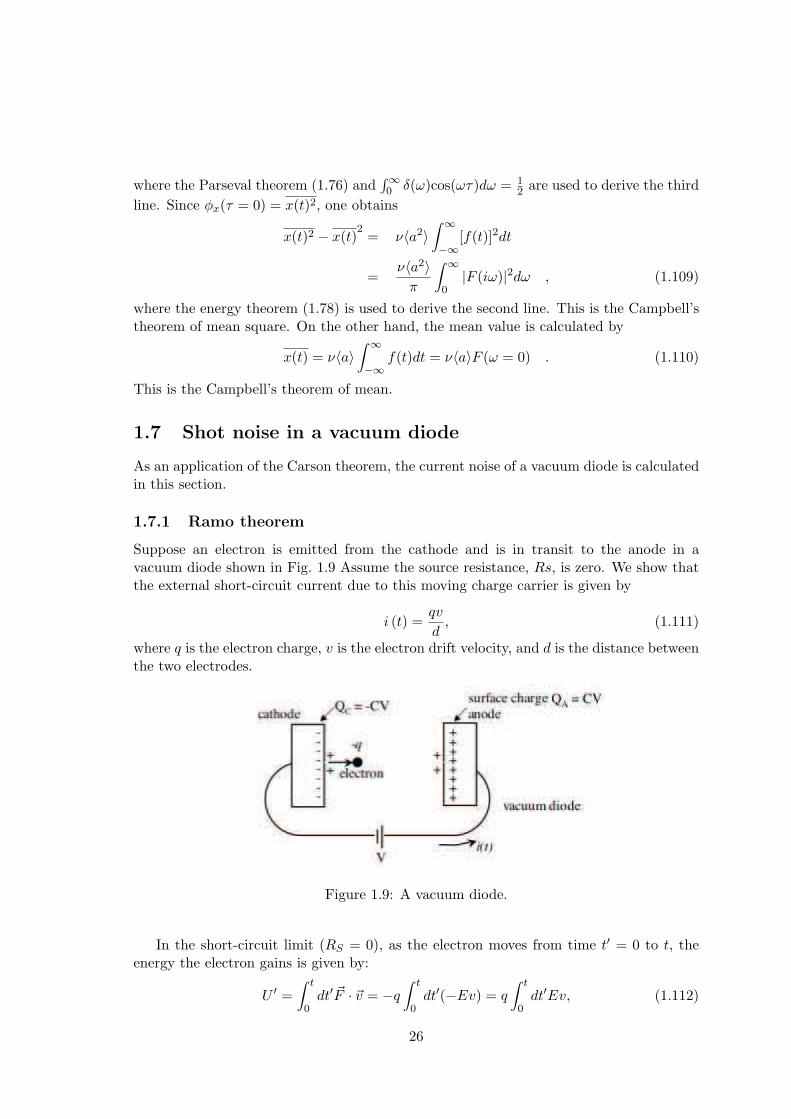
1.7.1 Ramo theorem

Suppose an electron is emitted from the cathode and is in transit to the anode in avacuum diode shown in Fig. 1.9 Assume the source resistance, Rs, is zero. We show thatthe external short-circuit current due to this moving charge carrier is given by

i (t) =qv

d, (1.111)

where q is the electron charge, v is the electron drift velocity, and d is the distance betweenthe two electrodes.

Figure 1.9: A vacuum diode.

In the short-circuit limit (RS = 0), as the electron moves from time t′ = 0 to t, theenergy the electron gains is given by:

U ′ =∫ t

0dt′ ~F · ~v = −q

∫ t

0dt′(−Ev) = q

∫ t

0dt′Ev, (1.112)

26

where F = qE is an external force acting on the electron and the electric field ~E is anti-parallel to ~v. If the current in the external circuit is i(t), the total energy supplied by theexternal voltage source is

U ′′ =∫ t

0dt′V (t′)i(t′) =

∫ t

0dt′V i(t′), (1.113)

where V (t) = V is constant. Since E = V/d in the tube, from U ′ = U” we obtain:∫ t

0dt′qEv =

∫ t

0dt′Edi(t′). (1.114)

Therefore we have Eq.(1.111). This is called the Ramo theorem.

1.7.2 External Circuit Current

We consider the case that the external circuit has a finite source resistance,Rs 6= 0, andthe circuit relaxation time, τc = RsC, is much longer than the electron transit time, τt,where C is the capacitance of the vacuum diode.

For τt = d/v ¿ τCR = RsC, the voltage developing due to the electron transit eventoccurs ”instantly,” whereas the relaxation through the external circuit is very slow. Im-mediately following the electron transit, the voltage across the vacuum diode is V − q/C,i.e., the voltage at anode is VA(t) = V − q/C at t = 0. Using Kirchoff’s law, and notingthat a current from battery to anode must be equal to a change in the surface charge, wehave

V − VA(t)Rs

=d

dt(CVA(t)). (1.115)

We rewrite (6) asd

dtVA(t) = −VA(t)

RsC+

V

RsC, (1.116)

and obtain the solution with the initial condition at t = 0 as

VA(t) = V − q

Ce−t/RsC . (1.117)

The current in the external circuit is then

i(t) =V − VA

Rs=

q

RsCe−t/RsC . (1.118)

1.7.3 Surface Charge

We now calculate the surface charges of the cathode and the anode as a function of timefor a single-electron traversal process in the following three cases:

(I) The electron drift velocity is assumed to be constant over the electron’s transit fromthe cathode to the anode, and τc ¿ τt.

(II) The electron drift velocity is initially zero at the cathode and is accelerated by theconstant applied electric field, and τc ¿ τt.

27

(III) τc À τt. In this case, we assume the electron transit to be an impulsive event.

(I)τc ¿ τt(Rs = 0) limit, constant vSince there is a voltage of V across the vacuum diode, there is a surface charge of CV

on the anode and −CV on the cathode. When an electron with charge −q is emitted fromthe cathode, it induces a net charge of +q on the cathode. Over the time, d/V , this chargeis compensated by the current supplied from the external circuit. The surface charge onthe cathode is:

Qc(t) = −CV + q −∫ t

0dt′i(t′). (1.119)

We perform the integration and obtain,

Qc(t) =

{−CV + q(1− v

d t) 0 < t < dv .

−CV otherwise(1.120)

The surface charge on the anode starts increasing by +q over the time d/v, due to theexternal current, from its t = 0 value of CV . Then, it is compensated for by the electronfrom the cathode. The surface charge on the anode is,

QA(t) = CV +∫ t

0dt′i(t′) =

{CV + q v

d t 0 < t < dv .

CV otherwise(1.121)

Since the external voltage source supplies an external current (without delay) to keep upwith the change inside the diode, the voltage across the diode is kept constant.

(II)τc ¿ τt(R = 0) limit, accelerated νNow we allow the electron to be accelerated by the electric field. The electron acquires

a velocity,

ν(t) =1m

p(t)1m

∫ t

0dt′F (t′) =

qE

mt. (1.122)

The transit time across the vacuum diode is,

dr

dt= v(t). (1.123)

This leads to,∫ d

0dr =

∫ Ttr

0dt′v(t′), Ttr =

√2md2

qV. (1.124)

The current can then be calculated from the current density.

J(t) =q

Adv(t), i(t) = J(t) ·A =

q

dv(t) =

q2V

md2t. (1.125)

The surface charge on the cathode is,

Qc(t) = −CV + q −∫ t

0dt′i(t′) (1.126)

=

{−CV + q

(1− qV

2md2 t2)

= −CV + q(1− v(t)

2d t)

0 < t < Ttr.

−CV otherwise(1.127)

28

The surface charge on the anode starts increasing by +q over the time Ttr, due to theexternal current, from its t = 0 value of CV . Then, it is compensated by the electronfrom the cathode. The surface charge on the cathode is:

QA(t) = CV +∫ t

0dt′i(t′) (1.128)

=

{CV + q2V

2md2 t2 = CV + qv(t)2d t 0 < t < Ttr.

CV otherwise(1.129)

Since the external voltage source supplies an external current (without delay) to keep upwith the change inside the diode, the voltage across the diode is still kept constant.

(III) τt ¿ τC limit, impulsive electron transitThe charge on the anode is given by

QA(t) = CVA(t) =

{CV − qe−t/RsC t > 0CV t < 0.

(1.130)

and that on the cathode is,

QC(t) = −CVA(t) = −QA(t) =

{−CV + qe−t/RsC t > 0−CV t < 0.

(1.131)

Here, the voltage across the diode has an RsC relaxation form.

1.7.4 Independent Emission of Electrons: a Poisson Point Process

For the case where the electron emission event and the transport process are mutuallyindependent, i.e. the electron emission obeys a Poisson point process. We calculate theexternal current noise spectra for the above three cases.

(I) τC ¿ τt(Rs = 0) limit, constant vThe Carson theorem states that for a random pulse train i(t) =

∑Kk=1 akf(t− tk) with

an identical pulse shape f(t), the unilateral power spectrum is given by,

S(ω) = 2ν〈a2k〉|F (iω)|2 + 4π

[νak

∫ ∞

−∞dtf(t)

]2

δ(ω), (1.132)

where ν is the average rate of arrival and F (iω) is the Fourier transform of f(t). In thiscase, each current pulse is given by

f(t) =

{q v

d 0 < t < dv ,

0 otherwise(1.133)

and the Fourier transform is

F (iω) =∫ ∞

−∞dtf(t)e−iωt =

∫ d/v

0dt

qv

de−iωt (1.134)

=qv(1− e−iωd/v)

iωd= qe−iωd/2v sin(ωd/2v)

(ωd/2v). (1.135)

29

Using (1.132), we obtain

Si(ω) = 2νq2 sin2(ωd/2ν)(ωd/2v)2

+ 4πv2q2δ(ω). (1.136)

Since the average rate is ν, the current is given by I = qν. Therefore (1.136) can bewritten as

Si(ω) = 2qI [sinc(ωd/2v)]2 + 4πI2δ(ω). (1.137)

In the low-frequency limit, 0 < ω ¿ v/d, since limx→0sin x

x = 1, we have

Si(ω ¿ 2v/d) = 2qI, (1.138)

which is a full shot noise.

(II) τC ¿ τt(Rs = 0) limit, accelerated vIn this case, each current pulse is given by

a =q2V

d2mand f(t) =

{t 0 < t < Ttr

0 otherwise.(1.139)

It follows that:

I = i(t) = a1

Ttr

∫ Ttr

0dt′f(t′) =

aνT 2tr

2= qν, (1.140)

〈a2〉 = a2, (1.141)

F (iω) =∫ ∞

−∞dtf(t)e−iωt =

∫ Ttr

0dtte−iωt = iTtr

e−iωTtr

ω− 1− e−iωTtr

ω2, (1.142)

where an integration by parts is used in the last line. The magnitude squared is,

|F (iω)|2 =2 + ω2T 2

tr − 2ωTtr sin(ωTtr)− 2 cos(ωTtr)ω4

. (1.143)

Plugging into the unilateral power spectral density as per the Carson theorem, we have

Si(ω) = 2ν

(q2V

d2m

)2 [2 + ω2T 2

tr − 2ωTtr sin(ωTtr)− 2 cos(ωTtr)ω4

]+ 4πν2q2δ(ω). (1.144)

We use

sin(ωTtr) = ωTtr − 13!

(ωTtr)3 + O(ω5), (1.145)

cos(ωTtr) = 1 +12!

(ωTtr)2 +14!

(ωTtr)4 + O(ω6), (1.146)

in the small frequency limit, to write the power spectral density as

Si(ω) = 2ν

(q2V

d2m

)2 (23!

T 4tr −

24!

T 4tr + O(ω5)

)+ 4πν2q2δ(ω). (1.147)

30

In the low-frequency limit, we ignore O(ω5), and we have

Si(ω) = 2qI + 4πI2δ(ω). (1.148)

In the low-frequency limit, 0 < ω ¿ 1/Ttr, the power spectral density is,

Si(ω ¿ 1Ttr

) = 2qI, (1.149)

which is again a full shot noise.

(III) τt ¿ τC limit, impulsive electron transitIn this case, each current pulse is given by

f(t) =

{q

CRse−t/RsC t > 0

0 t < 0,(1.150)

and the Fourier transform is

F (iω) =∫ ∞

−∞dtfiii(t)e−iωt =

q

1 + iωRsC. (1.151)

The power spectral density is then,

Si(ω) = 2νq2

1 + ω2R2sC

2+ 4πν2q2δ(ω) = 2qI

11 + ω2R2

sC2

+ 4πI2δ(ω). (1.152)

In the low-frequency limit, 0 < ω ¿ 1/RsC,

Si(ω ¿ 1/RsC) = 2qI, (1.153)

which is again a full shot noise.

1.7.5 Noise Suppression in Vacuum Diodes

For statistically independent emission of an electron to occur, the condition for electronemission has to be identical for each emission event. For the case in which τt À τC withconstant electron velocity, the relevant time scale is the electron transit time τt = d/v. Toensure statistical independence, we would require that no electron be emitted while oneis currently in transit through the vacuum. Incidentally, this is over the time scale forwhich the voltage across the vacuum diode is recovered to its initial value. Therefore, inthis case, we would require the electron emission rate to be

ν ¿ 1τt

(1.154)

for statistically independent emission of electrons. In the other limit,τC À τt, we realizethat the above condition is not satisfied. This is because the voltage across the vacuumdiode is not recovered within time τt after the electron emission event. The rate of electronemission would be a function of the voltage across the diode, and is only fully recovered

31

after a time τC has elapsed. Only then is the emission condition identical to ensurestatistically independent emission. Thus, we require the emission rate to be,

ν ¿ 1τC

(1.155)

If these conditions are not met, then there is a statistical dependence between the electronemission events. In this system, this dependence manifests itself as a negative feedbackprocess in which subsequent electron emissions are suppressed following an electron emis-sion. This is due to:

1. a space-charge effect in the τt À τC limit, in which the existence of an electron in thevacuum creates a repulsive potential such that the rate of the subsequent electronemissions is suppressed.

2. a memory effect in the external circuit in the τC À τt limit, in which the slowrecovery of the voltage across the diode suppresses the rate of the subsequent electronemissions.

In both cases, the tendency is to regulate the emission events. This regulation leads to aquieter stream of electrons, and the noise is suppressed below the full shot noise value.

32

Bibliography

[1] M. J. Buckingham, “Noise in Electronic Devices and Systems” (Ellis Horwood Pub.,1983).

[2] A. W. Drake, “Fundamentals of Applied Probability Theory” (McGraw-Hill, NewYork, 1988).

[3] A. Ambrozy, “Electronic Noise” (McGraw-Hill, New York, 1982).

[4] R. E. Burgess, Ed., “Fluctuation Phenomena in Solids” (Academic Press, New York,1965).

[5] D. F. Mix, “Random Signal Processing” (Prentice Hall, Englewood Cliffs, 1995).

[6] A. van der Ziel, “Noise in Solid State Devices and Circuits” (John Wiley & Sons,New York, 1986).

33