Mathematical modeling of semiconductor quantum …jinnliu/pub/2012NanoMMTA-qd.pdfMathematical modeling of semiconductor quantum ... density functional theory (DFT) ... B is the Bohr

Nanoscale Systems MMTA • ISSN: 2299-3290Survey Article • DOI: 10.2478/nsmmt-2012-0005 • NanoMMTA • Vol. 1 • 2012 • 58-79

Mathematical modeling of semiconductor quantumdots based on the nonparabolic effective-massapproximation

AbstractWithin the effective mass and nonparabolic band theory, ageneral framework of mathematical models and numericalmethods is developed for theoretical studies of semiconduc-tor quantum dots. It includes single-electron models andmany-electron models of Hartree-Fock, configuration interac-tion, and current-spin density functional theory approaches.These models result in nonlinear eigenvalue problems froma suitable discretization. Cubic and quintic Jacobi-Davidsonmethods of block or nonblock version are then presented forcalculating the wanted eigenvalues that are clustered in theinterior of the spectrum and may have small gaps and de-generacy. These are challenging issues arising from mod-eling a great variety of semiconductor nanostructures fabri-cated by advanced technology in semiconductor industry andscience. Generic algorithms for many-electron simulationsunder this framework are also provided. Numerical resultsobtained within this framework are summarized to three em-inent aspects, namely, accuracy of models, physical novelty,and effectivity of nonlinear eigensolvers. Concerning numer-ical accuracy, important details related to experimental dataare also addressed.

KeywordsQuantum dots • electronic structure • quantum models • non-linear eigenproblems • Jacobi-Davidson method.

PACS: 73.21.La, 73.23.Hk, 78.67.HcMSC: 65N06, 65F15© Versita sp. z o.o.

Jinn-Liang Liu∗

Department of Applied Mathematics, National Hsinchu University ofEducation, Hsinchu 300, Taiwan

Received 5 September 2012Accepted in revised form 15 October 2012

1. IntroductionSemiconductor quantum dots (QDs) are man-made nanostructures that typically consist of 103 to 109 atoms withequivalent number of electrons [52]. They are used to confine free electrons ranging from single to several hundredsin all three space dimensions and hence regarded as artificial atoms for their quantum analogies to natural atoms butwith controllable spectrum of energies for adding or removing electrons [2, 44, 52]. Rapid and far-reaching advances inunderstanding their electronic structure [70], transport phenomena [85], optical properties and quantum spin properties[32] etc. have been achieved significantly since the term ‘quantum dot’ was coined in 1988 [69]. Researchers havestudied QDs in a wide range of applications from transistors [26], lasers [8], solar cells [50], biological imaging [40],medical diagnostics [60], to quantum computing [56].On the other hand, a hierarchy of theories in solid state physics from Schrödinger, Bloch, Kronig-Penny, Wannier,Hartree-Fock, Slater, Thomas-Fermi, to Kohn-Sham have been applied to develop a great deal of mathematical models∗ E-mail: [email protected]

· NanoMMTA · Vol. 1 · 2012 · 58-79· 58Authenticated | [email protected] author's copy

Download Date | 11/17/12 11:22 AM

Mathematical modeling of semiconductor quantum dots

from tight-binding [18, 46, 47], configuration interaction [12, 13, 21, 59, 67, 72, 81, 82], density functional theory (DFT)[41, 55, 57, 75, 84], multiband [64, 68, 79], to one-band [4, 15, 22, 23, 29, 34, 51, 54, 74, 88, 89, 95] to study QD systems.No attempt is made in this article to review or compare vast results published in the literature of QD modeling. Forcomprehensive reviews in this aspect, we refer to [1, 5, 9, 10, 46, 47, 58, 62, 70, 91, 96] for more references.We survey instead a class of one-band envelope-function models that are based on the nonparabolic dispersion andeffective-mass approximation. These models are formulated in a framework setting for single-electron and many-electronQD simulations. Hartree-Fock (HF), configuration interaction (CI), and Kohn-Sham (KS) theories are used to developthe many-electron models. It is obvious that many-body QD simulations using HF, CI, or KS approach based on a fullscale of multiband structures are much more complicated in implementation and computationally expensive than thoseof one-band structures.Generic algorithms concerning numerical solution of eigenvalue problems, calculation of Coulomb integrals, andsimulation procedures are also provided. The most salient part of this framework is a particular type of nonlineareigenvalue problems for which the wanted eigenvalues are clustered in the interior of the spectrum that in turn lies inthe complex plane. Moreover, the eigenvalues may have very small gaps or even be degenerate. These issues are infact major challenges in the development of state-of-the-art eigensolvers for modeling large scale nano-systems [87].Nonlinear Jacobi-Davidson methods of both nonblock and block type are presented here in template style for tacklingthese problems and for motivating future studies. There are many other important issues such as linear scaling ofKS or HF calculations [28], multiscale and multiphysics modeling [58, 62], parallel implementation [46], and variousdiagonalization methods for many-body simulations [53] etc. that will not be addressed here.Numerical results obtained by our group within this framework are summarized into three examples in terms ofaccuracy of models [13, 34, 55], physical novelty [55, 88, 89, 95], and effectivity of nonlinear eigensolvers [36–38, 55, 92].The examples together with important details related to experimental data provide a synthetic view on how to performmany-electron QD simulations with advanced nonlinear eigensolvers.Considering fundamental impacts on nanoscale science, engineering, and technology by powerful and rapidlyadvancing simulation tools that go hand in hand with experimental developments, it is worthwhile to mention researchsoftware packages such as nextnano [9], NEMO [46, 47], and QUANTUM ESPRESSO [27] to name just a few thatare available to public access. All these packages are more general than ours in application, modeling, numerical, andcomplexity aspects. Nevertheless, our eigensolvers, an essential kernel of QD simulators, are rather effective for certainQD models and may be useful to the QD software development community. We shall integrate our solvers into a moreuser friendly package for the community in the future as a supplemental material to the present paper.The remaining part of the paper is organized as follows. We begin with single-electron models in Section 2 onwhich the general framework is built. Many-electron models using HF, CI, and DFT approaches are then formulated inSection 3. Numerical methods for nonlinear eigenproblems and simulation algorithms are presented in Section 4 wherephysical and mathematical results are also given. We then make some concluding remarks in Section 5.2. Single-Electron ModelsIn a bulk crystal of semiconductor material, the Hamiltonian for a noninteracting electron moving in a periodicpotential V (r) is

H0 = −~22m0∇2 + V , (1)where ~ is the reduced Planck constant, m0 is the free electron mass, and ∇ stands for the spatial gradient operator.For a given value of the crystal momentum p = ~k = −i~∇ where k is the Bloch wave vector, there are many discreteenergies εnk labeled by the band index n that an electron may have. For many electronic properties of semiconductor,we are only interested in a small k = |k| range around some extrema of the band structure of εnk instead of the wholeBrillouin zone. By the Bloch theory [5], the original Hamiltonian (1) can be transformed to the k · p Hamiltonian

Hkp = −~22m0∇2 + ~k · pm0 + ~2k22m0 + V (2)

that is defined in the smaller first Brillouin zone. By combing multiple bands to one band, we can further simplify theHamiltonian to an effective-mass approximationH∗ = −~22m∗∇2 + Vc(r), (3)



J.-L Liu

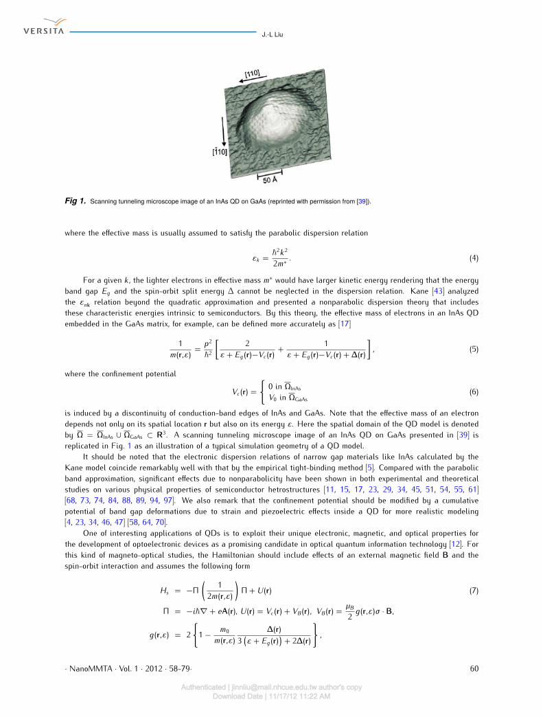
Fig 1. Scanning tunneling microscope image of an InAs QD on GaAs (reprinted with permission from [39]).

where the effective mass is usually assumed to satisfy the parabolic dispersion relationεk = ~2k22m∗ . (4)

For a given k , the lighter electrons in effective mass m∗ would have larger kinetic energy rendering that the energyband gap Eg and the spin-orbit split energy ∆ cannot be neglected in the dispersion relation. Kane [43] analyzedthe εnk relation beyond the quadratic approximation and presented a nonparabolic dispersion theory that includesthese characteristic energies intrinsic to semiconductors. By this theory, the effective mass of electrons in an InAs QDembedded in the GaAs matrix, for example, can be defined more accurately as [17]1

m(r,ε) = p2~2[ 2ε + Eg(r)−Vc(r) + 1

ε + Eg(r)−Vc(r) + ∆(r)], (5)

where the confinement potentialVc(r) = 0 in ΩInAs

V0 in ΩGaAs (6)is induced by a discontinuity of conduction-band edges of InAs and GaAs. Note that the effective mass of an electrondepends not only on its spatial location r but also on its energy ε. Here the spatial domain of the QD model is denotedby Ω = ΩInAs ∪ ΩGaAs ⊂ R3. A scanning tunneling microscope image of an InAs QD on GaAs presented in [39] isreplicated in Fig. 1 as an illustration of a typical simulation geometry of a QD model.It should be noted that the electronic dispersion relations of narrow gap materials like InAs calculated by theKane model coincide remarkably well with that by the empirical tight-binding method [5]. Compared with the parabolicband approximation, significant effects due to nonparabolicity have been shown in both experimental and theoreticalstudies on various physical properties of semiconductor hetrostructures [11, 15, 17, 23, 29, 34, 45, 51, 54, 55, 61][68, 73, 74, 84, 88, 89, 94, 97]. We also remark that the confinement potential should be modified by a cumulativepotential of band gap deformations due to strain and piezoelectric effects inside a QD for more realistic modeling[4, 23, 34, 46, 47] [58, 64, 70].One of interesting applications of QDs is to exploit their unique electronic, magnetic, and optical properties forthe development of optoelectronic devices as a promising candidate in optical quantum information technology [12]. Forthis kind of magneto-optical studies, the Hamiltonian should include effects of an external magnetic field B and thespin-orbit interaction and assumes the following form

Hs = −Π( 12m(r,ε))Π + U(r) (7)

Π = −i~∇+ eA(r), U(r) = Vc(r) + VB(r), VB(r) = µB2 g(r,ε)σ · B,g(r,ε) = 21− m0

m(r,ε) ∆(r)3 (ε + Eg(r))+ 2∆(r) ,




where Π denotes the electron momentum operator, e is the proton charge, A(r) is the vector potential induced by themagnetic field B, µB is the Bohr magneton, g(r,ε) is the Landé factor, and σ denotes the Pauli spin matrices.The single-electron QD model problem under consideration is hence to seek the wave function φ(r) and energy εsatisfying the effective-mass Schrödinger equationHsφ = εφ (8)

and the interface conditions [φ] = 0 and [ 1m(r,ε)∇φ · n

] = 0, (9)where [φ] denotes the jump of φ across the interface Γ between two materials, i.e. Γ = ΩInAs∩ΩGaAs, and n is an outwardnormal unit vector on Γ. Suitable boundary conditions of the Dirichlet type for φ should also be prescribed on theboundary ∂Ω of Ω.3. Many-Electron ModelsOur discussion on many-electron QD models is strictly within the above effective-mass approximation theory whichallows us to model conduction electrons and holes in a QD as a decoupled interacting system from their backgroundenvironment that may consist of millions of atoms in crystalline structure. To describe a system of N electrons in a QDunder the influence of the Coulomb interaction, we write the total Hamiltonian H as a sum of single-particle operatorsHi and two-body operators Vij as

H = N∑i=1 Hi + 12 ∑

i 6=j Vij , (10)Hi = Hs (ri) , Vij = 1

D(ri) ∣∣ri − rj∣∣ , D(ri) = 4πε0ε(ri)

e2 ,

where the single-electron Hamiltonian Hs (ri) is defined by (7) for the ith electron, ε0 is the vacuum permittivity, andε(ri) is the dielectric constant of two III-V compounds. For the sake of simplicity in exposition, the mutual interactionbetween the electrons in the system is taken to be purely Coulombic.3.1. Hartree-Fock ApproachThe Hartree-Fock approach postulates that the many-electron wave function Ψ of N interacting electrons in a QDsystem can be written as a single Slater determinant

Ψ = 1√N!∣∣∣∣∣∣∣∣∣∣ψ1 (r1σ1) ψ2 (r1σ1) · · · ψN (r1σ1)ψ1 (r2σ2) ψ2 (r2σ2) · · · ψN (r2σ2)... ... ... ...ψ1 (rNσN ) ψ2 (rNσN ) · · · ψN (rNσN )

∣∣∣∣∣∣∣∣∣∣(11)

of spin-orbitals ψi (rjσj) = ψi(rj)χi(σj ) so that the Pauli principle is fulfilled. Here, ψi (rj) represents the ith one-electron wave function (space orbital) occupied by the jth electron whose spin state is χi(σj ) = δ1σj or δ−1σjwhere δkl isthe Kronecker delta of the two integers k and l. The spin variable σj takes a value of either +1 for spin-up or −1 forspin-down. This antisymmetric representation of the electronic wave function enables us to include quantum mechanicaleffects of correlation and exchange in the QD system.Denoting the coordinates rjσj by the shorthand notation j , the complete expectation value of the Hamiltonian (10)in an antisymmetrized state (11) is

〈Ψ |H|Ψ〉 =∑i

∑j

∫drjψ∗i (j)( −12m(rj ,εj )

)Π2ψi(j) + U(rj ) |ψi(j)|2· NanoMMTA · Vol. 1 · 2012 · 58-79· 61

Authenticated | [email protected] author's copyDownload Date | 11/17/12 11:22 AM

J.-L Liu

+∑i

∑j>i

∫dridrj

1D(ri) ∣∣ri − rj

∣∣ [|ψi(j)|2 ∣∣ψj (i)∣∣2 − ψ∗i (j)ψ∗j (i)ψi(j)ψj (i)] , (12)where the energy level εj of the jth orbital is obtained by solving the Hartree-Fock equation

Hsψj (r) + Jψj (r) + Kψj (r) = εjψj (r) (13)in which the mass m(r,εj ) depends on the unknown energy. The Coulomb operator J and the exchange operator K aredefined as

Jψj (r) = ψj (r)∑i

∫dri

|ψi (ri)|2D(r) |r− ri|

, (14)Kψj (r) = −

∑iδχiχjψi (r)∫ dri

ψ∗i (ri)ψj (ri)D(r) |r− ri|

. (15)Note that the integration is taken over the bounded domain Ω.

3.2. Configuration Interaction ApproachThe configuration interaction is a more accurate theory than the Hartree-Fock theory in which the wave functionis expressed as a linear combination of Slater determinants so that the instantaneous Coulomb correlation of electronsis taken into account.From single-particle picture to many-particle picture for QDs, we follow the theoretical framework developed byPietiläinen and Chakraborty in [67]. The wave functions φl of (8) are chosen to form a single-particle basis setB1 = |φl〉 = |l〉 : l = 1, 2, · · · , Ns (16)

with Ns being the total number of single-particle states undertaken. The larger Ns the more accurate many-electron wavefunction can be obtained. However, it is finite since the number of energy levels in a QD is finite due to the confinementpotential (6). This is fundamental difference between the present approach and that in [67] where a parabolic confinementof QDs is used and hence their Ns is theoretically unbounded. Consequently, the number of basis functions (of theassociated Laguerre polynomial) required by their approach is of the order of million in implementation. Nevertheless,accuracy of our approach is controlled not only by Ns but also by the number of grid points used in, for instance, thefinite difference approximation of (8).From this set, a basis BN for N interacting electrons in a QD can be constructed as a direct antisymmetrizedproduct of B1 of the formBN = A N⊗

j=1 B1 = |Li〉 : i = 1, 2, · · · , Nm , (17)where A denotes the antisymmetrization operator for the Slater determinant as (11) and Nm = CNs

N the binomialcoefficient of Ns and N . More specifically, the many-electron basis functions |Li〉 are Slater determinants defined as|Li〉 = A [|li1〉 ⊗ |li2〉 · · · ⊗ |liN 〉]

= 1√N!∣∣∣∣∣∣∣∣∣∣φli1 (r1) φli2 (r1) · · · φliN (r1)φli1 (r2) φli2 (r2) · · · φliN (r2)... ... ... ...φli1 (rN ) φli2 (rN ) · · · φliN (rN )

∣∣∣∣∣∣∣∣∣∣(18)

in which the spin variable is omitted for simplicity. The states of the interacting system are then expressed by thesuperposition of the non-interacting states (17) as|Ψ〉 = Nm∑

i=1 ci |Li〉 , (19)· NanoMMTA · Vol. 1 · 2012 · 58-79· 62



where the unknown coefficients ci are sought by minimizing the energy functional〈Ψ |H|Ψ〉 (20)

with respect to ci subject to the normalization condition〈Ψ|Ψ〉 = 1. (21)

As an example, we illustrate the above formalism by considering a simple two-electron system as follows:N = 2, Ns = 3, B1 = |φl〉 : l = 1, 2, 3 , Nm = C 32 = 3!2!1! = 3, (22)

B2 = A2⊗

q=1 B1 = |Li〉 : i = 1, 2, 3 , (23)|L1〉 = |l1 ; l2〉 = 1√2

∣∣∣∣∣ φ1 (r1) φ2 (r1)φ1 (r2) φ2 (r2)

∣∣∣∣∣ ,|L2〉 = |l1 ; l3〉 = 1√2

∣∣∣∣∣ φ1 (r1) φ3 (r1)φ1 (r2) φ3 (r2)

∣∣∣∣∣ ,|L3〉 = |l2 ; l3〉 = 1√2

∣∣∣∣∣ φ2 (r1) φ3 (r1)φ2 (r2) φ3 (r2)

∣∣∣∣∣ ,

|Ψ〉 = 3∑j=1 cj

∣∣Lj⟩ , (24)〈Ψ |H|Ψ〉 = ∫∫

dr1dr2( 3∑

i=1 cj∣∣Lj⟩∗)H( 3∑

i=1 cj∣∣Lj⟩) , (25)

〈Ψ|Ψ〉 = ∫∫dr1dr2 |Ψ (r1, r2)|2 = 1. (26)

Using the method of Lagrange multipliers, the minimization of (25) subject to (26) yields∂∂ci〈Ψ |H|Ψ〉 − ε 〈Ψ|Ψ〉 = 0, i = 1, 2, 3, (27)

∂∂ci〈Ψ |H|Ψ〉 = ∫∫

dr1dr2 |Li〉∗H 3∑

j=1 cj∣∣Lj⟩

+∫∫ dr1dr2

3∑j=1 cj

∣∣Lj⟩∗H|Li〉 , (28)

∂∂ci

ε 〈Ψ|Ψ〉 = 2ε 3∑j=1 cj

∫∫dr1dr2 |Li〉∗ ∣∣Lj⟩ , (29)



J.-L Liu

Hij = ⟨Li |H| Lj⟩ = ⟨Li ∣∣∣∣H1 +H2 + 12V12∣∣∣∣ Lj⟩ , (30)

〈L2 |H1| L3〉 = ∫∫dr1dr2L∗2H1L3

= 12∫∫

dr1dr2 [φ∗1 (r1)φ∗3 (r2)− φ∗1 (r2)φ∗3 (r1)]H1[φ2 (r1)φ3 (r2)− φ2 (r2)φ3 (r1)]= 12∫∫

dr1dr2 [φ∗1 (r1)φ∗3 (r2)− φ∗1 (r2)φ∗3 (r1)][φ3 (r2)H1φ2 (r1)− φ2 (r2)H1φ3 (r1)] , (31)

〈L2 |H2| L3〉 = 12∫∫

dr1dr2 [φ∗1 (r1)φ∗3 (r2)− φ∗1 (r2)φ∗3 (r1)][φ2 (r1)H2φ3 (r2)− φ3 (r1)H2φ2 (r2)] , (32)⟨L2∣∣∣∣12V12

∣∣∣∣ L3⟩ = 14

∫∫dr1dr2 [φ∗1 (r1)φ∗3 (r2)− φ∗1 (r2)φ∗3 (r1)] e2

D(r1)1|r1 − r2| [φ2 (r1)φ3 (r2)− φ2 (r2)φ3 (r1)] , (33)

H11 H12 H13H21 H22 H23H31 H32 H33

c1c2c3

= ε

c1c2c3

. (34)Therefore, the total energy of N electrons in the QD can be obtained by diagonalizing the linear eigenvalueproblem

Nm∑j=1(Hij − εδij

)cj = 0, (35)

where the eigenvectors c = [c1 c2 · · · cNm ]T are expansion coefficients and the eigenvalues ε are corresponding energiesof the interacting system. The finite confinement potential leads to a finite number of localized states as well as toenergetically higher delocalized states. When the influence of the delocalized states on the discrete QD spectrum isneglected, the eigenvalue problem (35) has a finite dimension and can be solved without further approximations.There is another more accurate CI approach. Instead of using the single-electron wave functions φl calculated from(8), we can also use the single-electron Hartree-Fock orbitals ψl obtained from (13) to form the basis set B1 as (16). Itis very expensive in numerical implementation due to the following numerical problems:(I) We have two nonlinear problems for this approach. The first one is the nonlinear eigenvalue problem originatedfrom the nonparabolic mass m(r,εj ) in (13). This problem is the main focus in Section 4, which is also unavoidable forthe simpler CI approach. The second nonlinear problem is associated with the nonlinear dependence of the HF orbitalψj on the Coulomb and exchange integrals (14)-(15).(II) Computation of the Coulomb and exchange integrals is the bottleneck of Hartree-Fock simulations. Theseintegrals are calculated only once for the simpler approach as illustrated by (33) and (34) whereas, for the expensiveapproach, they are repeatedly evaluated in an iterative and alternating process between solving (13) and updating(14)-(15) until self-consistent wave function and potential are found.




3.3. Density Functional ApproachThe density functional theory developed by Hohenberg, Kohn, and Sham [33, 49] is perhaps the most successfulquantum mechanical method in reducing the computational complexity to investigate the electronic structure of many-body systems in physics and chemistry within tolerable computer time and accuracy. Vignale and Rasolt [86] extendedDFT to the current-spin DFT (CSDFT) by including gauge fields in the energy functional. It has been widely used formodeling QDs in magnetic fields [41, 70, 75].The crux of DFT is that the electron density of a many-electron system contains almost all essential materialproperties of the system that otherwise should be calculated from a many-electron wave function. Kohn and Shamproposed using single-electron wave functions to define the electron density. In this formalism, the kinetic energy ofelectrons can be captured more successfully not only by the density but also by its gradients. In CSDFT, the electrondensity is decomposed into the spin-up (σ = ↑) and spin-down (σ = ↓) componentsρ(r) = ρ↑(r) + ρ↓(r) (36)

that satisfy the constraint ∫ ρσ (r)dr =Nσ with N↑ = (N + 2S) /2 and N↓ = (N − 2S) /2 where S is the total spin ofthese N electrons [70]. Let ψjσ be the single-electron wave function of an electron occupying the jσ state such thatρ↑(r) =∑

j

∣∣ψj↑∣∣ , ρ↓(r) =∑j

∣∣ψj↓∣∣ . (37)The ground state energy of the system is a variational functional of the density defined as

E (ρ) = T (ρ) + EB (ρ) + ∫ ρ(r) [Vc(r) + 12VH(r)]dr + EXC (ρ) . (38)Minimization of this functional by varying ψ∗jσ = φ∗j (r)χj (σ ) under the above constraint yields the Kohn-Sham equation

HσKSψjσ = εjσψjσ , j = 1, · · · , dN/2e (39)with the KS Hamiltonian

HσKS = −Π( 12m(r,εjσ ))Π + VB(r) + Vc(r) + VH(r) + VXC(r), (40)

whereT (ρ) =∑

j,σ

⟨ψjσ∣∣∣∣Π( 12m(r,εjσ )

)Π∣∣∣∣ψjσ⟩ (41)is the kinetic energy of the electrons,

VH(r) = 1D(r)

∫ ρ(r′)|r− r′|dr′ (42)

is the Hartree potential,VXC(r) = δ [ρεXC (ρ, γ)]

δρσ − jpρ · AXC (43)

is the exchange-correlation potential, and de is the ceiling function symbol. Herejp(r) =−i~e2m ∑

j,σ

[ψ∗jσ (r)∇ψjσ (r)− ψjσ (r)∇ψ∗jσ (r)] (44)



J.-L Liu

is the paramagnetic current density andAXC = 1

ρ

(∂∂y

δ [ρεXC (ρ, ζ)]δζ , − ∂

∂xδ [ρεXC (ρ, ζ)]

δζ , 0) (45)is the exchange-correlation vector potential assuming that the external magnetic field B is directed along the z-axis.For the exchange-correlation energy functional εXC, we adopt the form developed by Perdew and Wang [65] as

εXC (ρ, ζ) = εX (rs, ζ) + εC (rs, ζ) (46)with

εX (rs, ζ) = − 34πrs[9π4

]1/3 [(1 + ζ)4/3 + (1− ζ)4/3]2 , (47)εC (rs, ζ) = εC (rs, 0) + αC(rs) f (ζ)f ′′(0) (1− ζ4)

+ [εC (rs, 1)− εC (rs, 0)] f (ζ)ζ4, (48)where ζ = (ρ↑(r)−ρ↓(r)) /ρ(r) is the relative spin polarization, rs = ( 34πρ

)1/3 is the Wigner-Seitz radius, and the functionsf (ζ), εC (rs, 0), εC (rs, 1) and −αC(rs) are given in [65].In numerical implementation, it is useful to break the KS Hamiltonian into separate components as

HσKS = TS + TB + VB + Vc + VH + VX + VC (49)with the kinetic energy of each single electron being further split into

〈TS〉 = −~22m∫

Ω ψ∗jσ∇2ψjσ dr and 〈TB〉 = e22m∫

Ω ψ∗jσA2ψjσ dr. (50)Other energy terms are similarly defined. Note that VH, VX, and VC depend self-consistently on the density ρ.The total energy of that electron is then evaluated according to the formula

Ejσ = 〈TS〉+ 〈TB〉+ 〈VB〉+ 〈Vc〉+ 12 〈VH〉+ EX + EC. (51)Accuracy of the exchange energies can be verified by the ratio of 12 〈VH〉 to the absolute value of EX, which is about 2for two-electron atoms [35]. It has been theoretically shown in [24] that this ratio is exactly equal to 2 for a two-electronmodel for which the exchange-correlation energy and potential can be determined exactly in an external harmonicpotential. The total energy of the N electrons is therefore the sum of these individual energies.4. Numerical MethodsFor semiconductor QD models with hard-wall confinement potential, real-space discretization methods such as thefinite difference or finite element method are more suitable for numerical approximation. The potential profile makesessential difference between natural and artificial atomic systems in implementation. Since conduction electrons in aQD system are not confined to any specific nucleus of natural atom, the widely used basis functions in computationalquantum chemistry such as Slater-type orbitals and Gaussian functions for the calculation of Coulomb integrals are notfeasible for QD simulations. Therefore, we shall only consider the finite difference method and numerical basis functionsin the following discussion. As mentioned above, we are only concerned with the nonlinear eigenvalue problem and thecalculation of Coulomb and exchange integrals among many important issues in realistic simulations.· NanoMMTA · Vol. 1 · 2012 · 58-79· 66



4.1. Nonlinear Eigenvalue ProblemsDue to the nonparabolic effective mass (5), a finite difference discretization of (8) and (9) with the magnetic fieldB = 0 yields a cubic eigenvalue problem of the form

A(λ)x = (A0 + λA1 + λ2A2 + λ3A3) x = 0, (52)where an unknown eigenpair (λ, x) is an approximate solution of (εl, φl) of (2.8) for some energy level l at grid pointsrj ∈ Ω, i.e., the eigenvalue λ ≈ εl and xj ≈ φl(rj ) with xj being the jth component of the eigenvector x. If (5) is rewrittenas 1

m(r,ε) = 1m(r,λ) = cλ+ d(λ+ a) (λ+ b) (53)

with the constants a, b, c, and d being simplified from the physical parameters in (5), it can be seen that the matrixA0 is a combination of two matrices corresponding to the kinetic and potential terms in (7) together with the gradientinterface condition in (9), A1 is related to all three terms in (8), A2 is from the potential term and the right-hand side of(8), and A3 is an identity matrix from the right-hand side. Note that the Landé factor g(r,ε) in (7) will make the nonlineareigenvalue problem even further to the fifth order if B 6= 0.The cubic or quintic eigenvalue problem belongs to a more general family of polynomial eigenvalue problems [3].A variety of numerical methods [36–38, 90, 92] have been developed for solving this type of problems in recent yearsdue to their interesting mathematical and physical features.The cubic eigenproblem (52) can be transformed to the generalized linear eigenvalue problem 0 I 00 0 I

A0 A1 A2

xλxλ2x

= λ

I 0 00 I I0 0 −A3

xλxλ2x

. (54)This enlarged problem can be solved by various well-known methods such as the Lanczos or Arnoldi method. However,disadvantages of such an approach still exist. First of all, the order of the matrix is tripled and its condition numbermay increase drastically since the set of admissible perturbations for (54) is larger than that of (52) [83]. Secondly, theperformance of these methods may be reduced for the enlarged problem in terms of convergence and accuracy. Thirdly,Lanczos and Arnoldi methods require the use of the shift-and-invert technique for such a large sparse eigenvalue problemsince the desired eigenpairs are located in the interior of the spectrum of the problem. Consequently, the computationalcost for solving linear system is excessive.It can also be transformed to a fixed-point problem

F (λ)x = µG(λ)x (55)with, for instance,

F (λ) = −A1 + λA2 + λ2A3, G(λ) = A0, and µ = 1λ .

There are of course other choices for F (λ) and G(λ) [37]. A general algorithm for solving (55) consists of the followingtwo steps:Step 1. Solve F (λi)x = µG(λi)x by an eigensolver for the maximum eigenpair (µmax, xmax) with λi being given.Step 2. Update i = i+ 1; λi = 1/µmax where λ0 is an initial guess value. Go to Step 1 until convergence.Again there are many methods that can be used to implement the eigensolver. If λi is close to a desired eigenvalue,Step 1 can be accelerated by Newton’s method, namely, by solving the correction equationA(λi)x = µA′(λi)x (56)

for the minimum eigenpair (µmin, xmin) with an update λi+1 = λi−µmin instead of solving (55). Here A′(λi) is the derivativeof A(λ) at λi.There is another type of subspace methods such as the nonlinear Arnoldi and Jacobi-Davidson (JD) method forsolving (52) [38, 90]. A Jacobi-Davidson algorithm generally consists of the following steps.Algorithm 1. A Cubic Jacobi-Davidson Method.



J.-L Liu

(1) Choose an n×m initial orthonormal matrix V (a subspace) where n is the matrix size of (52) and m << n.(2) Form smaller matrices Wi = AiV and Mi = V ∗Wi for i = 0, 1, 2, 3.(3) Solve the smaller cubic eigenproblem

(M0 + θM1 + θ2M2 + θ3M3) y = 0 (57)

for (θ, y) so that the Ritz pair (θ, z = Vy) ≈ (λ, x) is the wanted eigenpair.(4) Solve approximately the correction equation

(I − pz∗

z∗p

)A(θ) (I − zz∗) t = −r (58)

for t ⊥ z, where r = A(θ)z is the residual and p = A′(θ)z.(5) Expand V = [V , t]. Go to Step (2) until convergence or go to Step (1) for a restart.

Since the matrix size of the projected eigenproblem (57) is much smaller than that of (52), its transformation to alinear problem like (54) is now computationally feasible, which can then be solved by, for example, the QR method. Ofcourse, there are other alternatives for solving the subspace eigenproblem. The correction equation (58) is originatedfrom Jacobi’s idea. It is the most computationally demanding part in a JD algorithm for large matrix systems and thusshould be solved via some efficient preconditioner such as SSOR [38]. Nevertheless, it has been demonstrated in [7]that JD is highly sensitive to preconditioning and can display an irregular convergence behavior. It takes the form ofK t = r for the Arnoldi method [90] with K being a preconditioner such that K ≈ A(σ ) and σ is a pole close to a wantedeigenvalue.In addition to fundamental problems associated with these two basic principles of JD methods [77, 78], severalnumerical issues on (52) that arise from the physical properties of QDs need to be addressed. The wanted eigenvaluesare embedded in the interior of the eigenvalue spectrum in the complex plane, i.e. (λ, x) ∈ C × Cn, may be clusteredwith small gaps, and may have multiplicity larger than one [37].For seeking multiple eigenpairs, it is well known that a combination of JD and implicit deflation techniques basedon the Schur form can lead to effective algorithms for linear eigenproblems. However, the Schur form is in generalundefined for a cubic matrix pencil and hence the use of explicit deflation schemes is inevitable. In cases that twoconsecutive eigenvalues are close to each other, the explicit deflation scheme specific to linear eigenproblems may notbe stable due to ill-conditioned deflation matrices.More specifically, let (Λ, VF ) ∈ Rr×r × Rn×r be an eigenmatrix of A(λ) with V T

F VF = I , i.e. let r eigenpairs bealready found and henceA(Λ)VF = A0VF + A1VFΛ + A2VFΛ2 + A3VFΛ3 = 0. (59)

We then deflate Λ to infinity by defining a new deflated cubic eigenproblem asA(λ)x = (

A0 + λA1 + λ2A2 + λ3A3) x = 0, (60)A0 = A0,A1 = A1 − (A1VFV T

F + A2VFΛV TF + A3VFΛ2V T

F),

A2 = A2 − (A2VFV TF + A3VFΛV T

F),

A3 = A3 − A3VFV TF .

By (59) and (60), it can be shown that [38]A(θ) = A(θ)T (θ), T (θ) = I − θVFΛ−1V T

F , (61)· NanoMMTA · Vol. 1 · 2012 · 58-79· 68



where θ /∈ σ (Λ) the spectrum of Λ.The matrix T (θ) is called the deflation transformation matrix which may be ill-conditioned if θ is very close to anycomputed eigenvalue in σ (Λ). This means that a direct replacement of A(λ) by A(λ) in Algorithm 1 for calculating the nexteigenpair may incur instability or even divergence. Note that this kind of situation occurs inevitably for many-electronQD systems since the energy difference between spin-up and spin-down electrons (two eigenvalues) occupying the sameorbital state is very small and approaches zero as the magnetic field B tends to zero.Moreover, the computational cost for solving the deflated problem becomes more expensive as VF gets larger.Therefore, a key factor to develop robust and efficient JD methods for QD models is to solve the correction equation (58)not only approximately but also indirectly. For this, a more convenient formulation for (58) isA(θ)t = −r + αp (62)

from which one can have various ways for calculating the ‘stepping length’ α , for instance [38, 78],α = z∗K−1r

z∗K−1p , (63)where K is a preconditioner of A(θ). With this preconditioner, the correction equation (58) is replaced by

K t = −r + αp, p = [A′(θ)− A′(θ)T (θ)] z (64)for the next eigenpair.Block eigensolvers are commonly used in many-body simulations in computational quantum chemistry and physics[87, 93]. They are more efficient than nonblock methods for calculating multiple or clustered eigenvalues that areessentially originated from the interaction Hamiltonian of many-body systems. Moreover, they allow parallelism andefficient use of local memory [16, 25, 30, 48, 87, 98, 99]. A block method is more suitable for many-electron QD modelssince degeneracies and small gaps of eigenvalues cause slow convergence in the deflation procedure. For the DFTmodel (39) with the magnetic field B 6= 0, the block Davidson method of Crouzeix, Philippe, and Sadkane [16] can begeneralized to a block JD method as follows.

Algorithm 2. A Quintic Block Jacobi-Davidson Method.(1) Choose an n×m initial orthonormal matrix V where n is the matrix size of the quintic eigenproblem

A(λ)x = (A0 + λA1 + λ2A2 + λ3A3 + λ4A4 + λ5A5) x = 0 (65)corresponding to the N-electron KS equation (39) and m = dN/2e for both spin-up and spin-down states(m << n).

(2) Form smaller matrices Wi = AiV and Mi = V ∗Wi for i = 0, 1, · · · , 5.(3) For j = 1, 2, · · · , m,

(3a) solve the smaller quintic eigenproblem(M0 + θjM1 + θ2

jM2 + θ3jM3 + θ4

jM4 + θ5jM5) yj = 0 (66)

for (θj , yj ) so that the Ritz pair (θj , zj = Vyj ) ≈ (λj , xj ) is the wanted eigenpair,(3b) solve the preconditioned correction equationK t = −r + αp, (67)

r = A(θj )zj , α = z∗jK−1rz∗jK−1p , p = A′(θj )zj , t ⊥ zj , and



J.-L Liu

(3c) expand V = [V , t].(4) Go to Step (2) until convergence or go to Step (1) for a restart.

This is a general algorithm of a solution procedure for this kind of large and complicated nonlinear eigenproblems.There are of course many details missing in the algorithm such as restarting strategy, rank deficiency, adaptive blocksizes, numerical schemes for the subspace problem (66), effective preconditioners, and variants of the correction equationthat may affect the overall performance of the algorithm.For the CI approach, the basic step is to construct numerically the single-electron basis functions φl in (16). WithB 6= 0, one can apply either Algorithm 1 or 2 to the single-electron model (8) with a corresponding quintic eigenproblem.Again many details concerning the accuracy and efficiency of the construction and computation of the basis set remainto be investigated.4.2. Evaluation of Coulomb IntegralsWe now give a brief discussion on the calculation of Coulomb and exchange integrals in many-electron models.Since the many-electron basis functions |Li〉 in (18) lead to a Slater determinant of single-electron basis functions φlthat have been approximated via a JD algorithm which in turn renders a set of orthonormal eigenvectors, the matrixelements like (31) and (32) only involve the single-electron Hamiltonians H1 and H2 and hence their discrete forms aresimply diagonal matrix elements associated with the products of the eigenvectors. In other words, the computationallydemanding terms in the matrix elements Hij in (35) are those of Coulomb integrals like (33) for which we use the followinggeneric four-center two-electron repulsion formula

〈12|VC|34〉 = ∫∫Ω dr′drφ∗1(r)φ∗2(r′ ) 1D(r) |r− r′|φ3(r)φ4(r′ ), (68)

where VC denotes the two-body Coulomb operator and φi(r), i = 1, 2, 3, 4, represent any arbitrary four single-electronfunctions.For real space approximation, we define a potential-like functionV24(r) = 1

D(r)∫

Ωφ∗2(r′ )φ4(r′ )|r− r′| dr′ (69)

that can be obtained by solving the Poisson equation−∇ ·D(r)∇V24(r) = φ24 (r) , φ24 (r) = φ∗2(r)φ4(r). (70)

Again a finite difference approximation of (70) and (9) results in a matrix systemAx = b, (71)

where A is an n × n matrix that corresponds to the left-hand side of (70) and is different from A(λ), b corresponds toφ24 (r), and xj ≈ V24(rj ) with xj being the jth component of the unknown vector x. The literature on the development offast Poisson solvers is vast, see e.g. [14, 31, 71]. Note that, for DFT approach, the Hartree potential (42) can also becalculated by means of the Poisson equation

−∇ ·D(r)∇VH(r) = ρ (r) . (72)We summarize our discussion on numerical methods for many-electron QD simulations in the following two generalalgorithms via CI and DFT approaches.

Algorithm 3. A Configuration Interaction Approach for N-electron QD Simulation.· NanoMMTA · Vol. 1 · 2012 · 58-79· 70



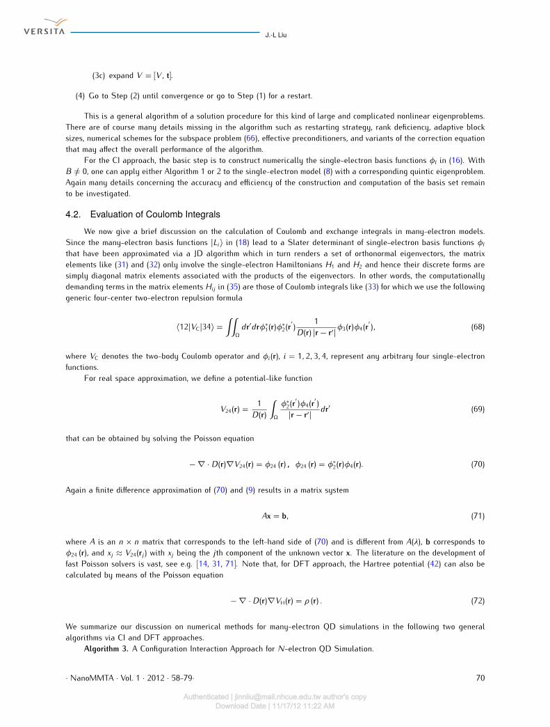
Fig 2. A cross section of an InAs/GaAs QD in nano meters.

(1) Solve the single-electron model (8) in discrete form (52) by Algorithm 1 or 2 for Ns basis functions in (16).(2) Form an Nm ×Nm interaction matrix H = [Hij

] as in (35) with Nm = CNsN by

(2a) calculating diagonal elements Hii via the inner product of eigenvectors in correspondence to (31), and(2b) calculating mixing elements Hij via solving (71) in correspondence to (33) by a suitable Poisson solver.(3) Solve the eigenproblem as (34) for the total energy ε and wave function Ψ (19) of the N electrons by a suitableeigensolver.

Algorithm 4. A Density Functional Theory Approach for N-electron QD Simulation.(1) Set VH = VXC = 0 and solve the KS equation (39) in discrete form (66) by Algorithm 2 with σ = ↑ and then σ =↓ to get ψjσ for j = 1, · · · , dN/2e.

(2) Evaluate all electron energies Ejσ by (51) and go to the next step until a self-consistent convergence is reached.(3) Update the electron densities ρ↑, ρ↓, and ρ in (36) and (37) with new ψjσ .

(3a) Solve (72) in discrete form (71) for a new VH by a suitable Poisson solver.(3b) Solve the KS equation (39) by Algorithm 2 for new ψjσ and then go to Step (2).4.3. Physical and Mathematical ResultsThe main purpose of this section is to present novel physical and mathematical results obtained in the past yearsunder this framework albeit its simplification and approximation in energy band structures [13, 34, 37, 38, 54, 55, 88,89, 92, 95]. For conciseness, we summarize our results to three noteworthy aspects.

A. Accuracy of Models. We first present results that are verified with experimental data to show the correctnessof our QD models. We consider an InAs/GaAs QD as shown in Fig. 1 where a 2D cross section is depicted in Fig. 2.The finite confinement potential is Vc = 0.77 eV and the effective potential acting upon the quantum dot volume isVs = 0.482 eV [22] to account the strain and piezoelectric effects. In order to verify the accuracy of the CSDFT model(39), numerical results are presented in an analogous way to that of [22] where the CV experimental data of [61] wereextracted for numerical studies.All numerical values of the parameters used in this paper are listed in Table 1.In Fig. 3, the capacitance-gate-voltage trace from [61] is shown. The peaks correspond to the occupation ofthe s-shell (E0) and p-shell (E1) energy levels by tunneled electrons with an increasing number of electrons, i.e.,N = 1, 2, · · · , 6. As mentioned in [61], the trace has been scaled by a multiplication factor (within about 30% accuracy)· NanoMMTA · Vol. 1 · 2012 · 58-79· 71


J.-L Liu

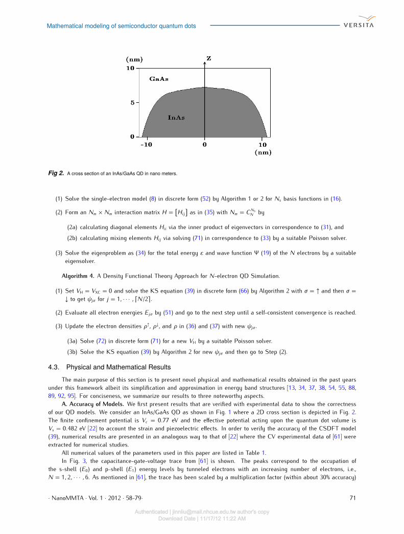
Table 1. Numerical values of the parameters.

Symbol Value Unitp (InAs) 1.20311× 10−28p (GaAs) 1.25614× 10−28m0 9.10956× 10−31 kgEg (InAs) 0.421 eVEg (GaAs) 1.52 eV∆ (InAs) 0.48 eV∆ (GaAs) 0.34 eVVc 0.77 eVε0 8.854187× 10−12 F/mεInAs 12.2εGaAs 12.7µB 9.2741× 10−24 J/T

Fig 3. The capacitance-gate-voltage trace where the capacitance is in arbitrary units. The peaks correspond to the occupation of the s and p energyshells by tunneled electrons. The arrows with E0, E1, E2 indicate the s, p, and d levels, respectively, obtained by the CV spectroscopy data[61]. Our results are denoted by E0, E1, E2.

and is offset for clarity. Note that at zero magnetic field the peak corresponding to the d-shell (E2) level is not presentin [61]. Since the precise values of these levels are not given in both [61] and [22], the experimental values E0 = 0.59,E1 = 0.642, and E2 = 0.69 eV are approximated by inspecting the data shown in the figures in [22]. Our numericalresults of the corresponding peak energies are E0 = 0.608, E1 = 0.65, and E2 = 0.701 that show good agreement withthe experimental results. Moreover, there are two small sub-peaks in the s peak and four in the p peak, which indicatesmall variations in total energy of the system as electrons are added to the QD one by one. Our capacitance profilealso shows these variations and is consistent with the experimental profile.We next compare the results obtained by parabolic and nonparabolic CSDFT methods for the 6-electron system ina magnetic field to show the importance of nonparabolic effect with respect to the magnetic field. In Fig. 4, the solid linesrepresent the results of the s, p, and d shells with various magnetic fields by the nonparabolic method while the dashedlines correspond to the parabolic method. We find that the nonparabolic effect is more pronounced in many-electron· NanoMMTA · Vol. 1 · 2012 · 58-79· 72



Fig 4. The s, p, and d levels within the confinement potential Vc = 0.77 eV in a magnetic field. All levels are obtained by CSDFT with nonparabolic(solid lines) and parabolic (dashed lines) effective-mass approximation.

system than in single-electron system. For example, for the p-shell levels at B = 20 T in Fig. 4, the Zeeman splittingof the parabolic case is ∆E = 70 meV which is much wider than ∆E = 47 meV of the nonparabolic case. By inspectingthe results of [22], the splitting for the nonparabolic single-electron model is ∆E = 42 meV. Obviously, the nonparabolicband effect is more important for the many-electron models than single ones. Note that the upper energy levels of thed-shell electron are not present in the figures of [22]. Furthermore, the energy level of the spin-down d-shell electron atB = 20 T obtained by the nonparabolic method is E2↓ = 0.758 eV which is still within the confinement potential well.It is, however, out of the confinement for the parabolic case.

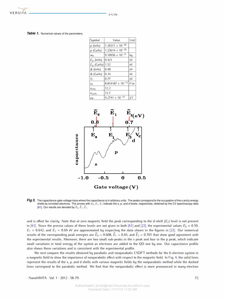
B. Quantum Entanglement. There is significant interest in quantum information processing based on Fermionicqubits using semiconducting materials [6, 19, 20, 42, 63]. One of the proposals in this approach is to exploit electronicinteractions of coupled quantum dots that form an artificial molecule (QDM) [6, 20, 63]. In QDM, one can adjust theinter-dot distance and through that to control coupling between electronic states localized in different dots. The abilityto control coherent coupling between quantum dots may open possibility for designing quantum logic gates [6, 63].The inter-dot distance control is an example of a static approach to the gate design. Another possibility to controldynamically the coupling lies in application of external fields [42].We demonstrate a theoretical model of quantum entanglement in a triple-dot artificial molecule via dynamic controlof magnetic or electric field. The QDM is a vertical stack of three InAs dots with two different sizes embedded in GaAsas depicted in Fig. 5 where the radius, thickness, and separation of each dot are indicated by coordinates in nano meters.These QD dimensions are commensurable with those of [63] where a transmission electron micrograph of a QDM sampleis illustrated. The magnetic field B is applied in the z-axis and the electric field is controlled by changing the voltage Vgof a circular Schottky gate surrounding the central dot as shown in blue in Fig. 5. The red part represents an insulator.We study the electronic configuration of N = 6 electrons confined in the QDM under these two fields by using theCSDFT approach.The entanglement is posited under two different field conditions. Case 1: Vg = 0 V and B = 0 to 15 T. The leftpanel of Fig. 6 consists of three frames in which the configuration of 6 electrons in QDM with B = 0 is illustrated. Eachframe represents a contour of the wave function of 2 electron (spin-up and spin-down). These three frames indicate thatall 6 electrons are located in the central dot. We denote this 6-electron state in the QDM by 〈0|. The right panelof the figure corresponds to B = 15 T. Each dot of the QDM contains two electrons as shown by the contour in each· NanoMMTA · Vol. 1 · 2012 · 58-79· 73


J.-L Liu

Fig 5. A radial cross-section of three vertically aligned InAs quantum dots (a QDM) embedded in GaAs.

Fig 6. Case 1. Vg = 0 V. Left panel: B = 0. Each frame represents the contour of the wave function of two electrons (spin-up and -down). All 6electrons are in the central dot. Right panel: B = 15 T. Each dot contains two electrons.

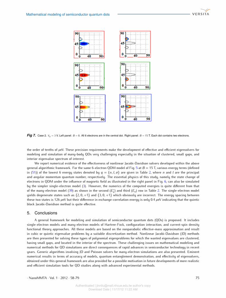
frame. This state is then denoted by 〈1|. These results show that we may be able to control electrons in a QDM byvarying the magnetic field so that an entangled state α 〈0|+ β 〈1| with α 6= 0 and β 6= 0 for quantum computing can beestablished. Similar results are found for Case 2: Vg = 3 V and B = 0 to 15 T as shown in Fig. 7.C. Effectivity of Eigensolvers. Experimental implementations of quantum information processing with semicon-ductor QDs require the measurement accuracy of energy spectrum be as small as in the order of tens of µeV. Forexample, the spectral resolution of a N2-cooled Si-CCD camera is 80 µeV for detecting the optical emission of a QDexciton by a continuous wave laser in the study of the excitonic transitions of QDs [66]. On the other end, theoreticalimplementations in, for instance, our DFT model setting, require the numerical accuracy of the correlation energy be in




Fig 7. Case 2. Vg = 3 V. Left panel: B = 0. All 6 electrons are in the central dot. Right panel: B = 15 T. Each dot contains two electrons.

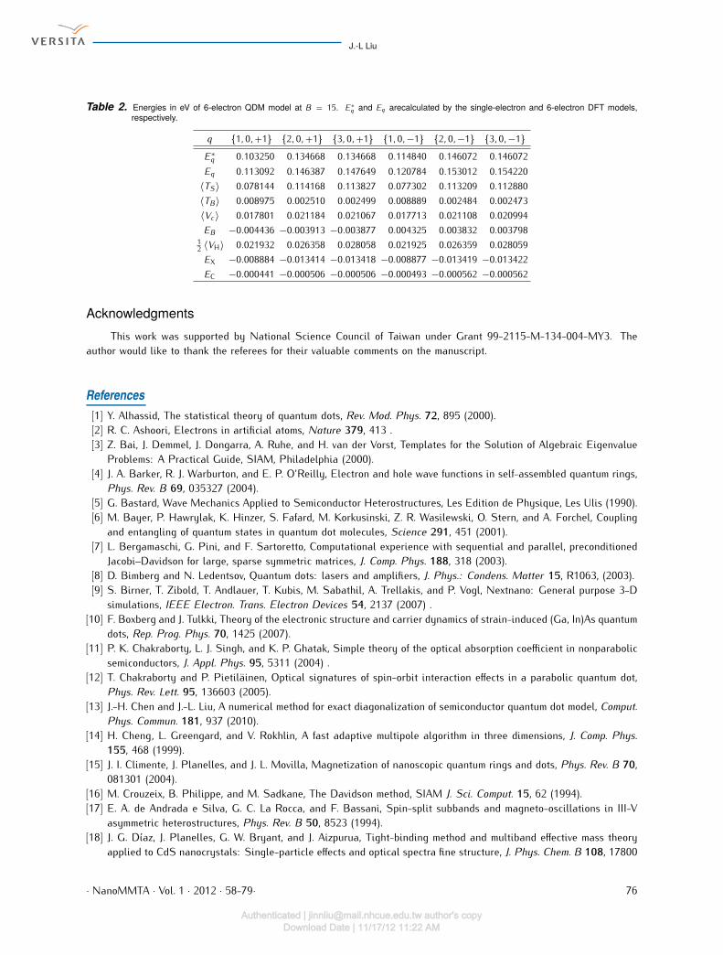
the order of tenths of µeV. These precision requirements make the development of effective and efficient eigensolvers formodeling and simulation of many-body QDs very challenging especially in the situation of clustered, small gaps, andinterior eigenvalue spectrum of interest.We report numerical evidence of the effectiveness of nonlinear Jacobi-Davidson solvers developed within the abovegeneral algorithmic framework. For the same 6-electron QDM model of Fig. 5 at B = 15 T, various energy terms (definedin (51)) of the lowest 6 energy states denoted by q = n, l, σ are given in Table 2, where n and l are the principaland angular momentum quantum number, respectively. The essential physics of this study, namely the state change ofelectrons in QDM under the influence of magnetic field as illustrated in the right panel in Fig. 6, can also be simulatedby the simpler single-electron model (3). However, the numerics of the computed energies is quite different from thatof the many-electron model (39) as shown in the second (E∗q) and third (Eq) row in Table 2. The single-electron modelyields degenerate states such as 2, 0,+1 and 3, 0,+1 which obviously are incorrect. The energy spacing betweenthese two states is 126 µeV but their difference in exchange-correlation energy is only 0.4 µeV indicating that the quinticblock Jacobi-Davidson method is quite effective.5. ConclusionsA general framework for modeling and simulation of semiconductor quantum dots (QDs) is proposed. It includessingle-electron models and many-electron models of Hartree-Fock, configuration interaction, and current-spin densityfunctional theory approaches. All these models are based on the nonparabolic effective-mass approximation and resultin cubic or quintic eigenvalue problems by a suitable discretization method. Nonlinear Jacobi-Davidson (JD) methodsare then presented for solving these types of polynomial eigenproblems for which the wanted eigenvalues are clustered,having small gaps, and located in the interior of the spectrum. These challenging issues on mathematical modeling andnumerical methods for QD simulations are direct consequences of rapid advances in semiconductor technology in recentyears. Generic algorithms involving JD and Poisson solvers for many-electron simulations are also presented. Eminentnumerical results in terms of accuracy of models, quantum entanglement demonstration, and effectivity of eigensolvers,obtained under this general framework are also provided for a possible motivation in future developments of more realisticand efficient simulation tools for QD studies along with advanced experimental methods.· NanoMMTA · Vol. 1 · 2012 · 58-79· 75


J.-L Liu

Table 2. Energies in eV of 6-electron QDM model at B = 15. E∗q and Eq arecalculated by the single-electron and 6-electron DFT models,respectively.

q 1, 0,+1 2, 0,+1 3, 0,+1 1, 0,−1 2, 0,−1 3, 0,−1E∗q 0.103250 0.134668 0.134668 0.114840 0.146072 0.146072Eq 0.113092 0.146387 0.147649 0.120784 0.153012 0.154220〈TS〉 0.078144 0.114168 0.113827 0.077302 0.113209 0.112880〈TB〉 0.008975 0.002510 0.002499 0.008889 0.002484 0.002473〈Vc〉 0.017801 0.021184 0.021067 0.017713 0.021108 0.020994EB −0.004436 −0.003913 −0.003877 0.004325 0.003832 0.00379812 〈VH〉 0.021932 0.026358 0.028058 0.021925 0.026359 0.028059EX −0.008884 −0.013414 −0.013418 −0.008877 −0.013419 −0.013422EC −0.000441 −0.000506 −0.000506 −0.000493 −0.000562 −0.000562

AcknowledgmentsThis work was supported by National Science Council of Taiwan under Grant 99-2115-M-134-004-MY3. Theauthor would like to thank the referees for their valuable comments on the manuscript.References[1] Y. Alhassid, The statistical theory of quantum dots, Rev. Mod. Phys. 72, 895 (2000).[2] R. C. Ashoori, Electrons in artificial atoms, Nature 379, 413 .[3] Z. Bai, J. Demmel, J. Dongarra, A. Ruhe, and H. van der Vorst, Templates for the Solution of Algebraic EigenvalueProblems: A Practical Guide, SIAM, Philadelphia (2000).[4] J. A. Barker, R. J. Warburton, and E. P. O’Reilly, Electron and hole wave functions in self-assembled quantum rings,

Phys. Rev. B 69, 035327 (2004).[5] G. Bastard, Wave Mechanics Applied to Semiconductor Heterostructures, Les Edition de Physique, Les Ulis (1990).[6] M. Bayer, P. Hawrylak, K. Hinzer, S. Fafard, M. Korkusinski, Z. R. Wasilewski, O. Stern, and A. Forchel, Couplingand entangling of quantum states in quantum dot molecules, Science 291, 451 (2001).[7] L. Bergamaschi, G. Pini, and F. Sartoretto, Computational experience with sequential and parallel, preconditionedJacobi–Davidson for large, sparse symmetric matrices, J. Comp. Phys. 188, 318 (2003).[8] D. Bimberg and N. Ledentsov, Quantum dots: lasers and amplifiers, J. Phys.: Condens. Matter 15, R1063, (2003).[9] S. Birner, T. Zibold, T. Andlauer, T. Kubis, M. Sabathil, A. Trellakis, and P. Vogl, Nextnano: General purpose 3-Dsimulations, IEEE Electron. Trans. Electron Devices 54, 2137 (2007) .[10] F. Boxberg and J. Tulkki, Theory of the electronic structure and carrier dynamics of strain-induced (Ga, In)As quantumdots, Rep. Prog. Phys. 70, 1425 (2007).[11] P. K. Chakraborty, L. J. Singh, and K. P. Ghatak, Simple theory of the optical absorption coefficient in nonparabolicsemiconductors, J. Appl. Phys. 95, 5311 (2004) .[12] T. Chakraborty and P. Pietiläinen, Optical signatures of spin-orbit interaction effects in a parabolic quantum dot,Phys. Rev. Lett. 95, 136603 (2005).[13] J.-H. Chen and J.-L. Liu, A numerical method for exact diagonalization of semiconductor quantum dot model, Comput.Phys. Commun. 181, 937 (2010).[14] H. Cheng, L. Greengard, and V. Rokhlin, A fast adaptive multipole algorithm in three dimensions, J. Comp. Phys.155, 468 (1999).[15] J. I. Climente, J. Planelles, and J. L. Movilla, Magnetization of nanoscopic quantum rings and dots, Phys. Rev. B 70,081301 (2004).[16] M. Crouzeix, B. Philippe, and M. Sadkane, The Davidson method, SIAM J. Sci. Comput. 15, 62 (1994).[17] E. A. de Andrada e Silva, G. C. La Rocca, and F. Bassani, Spin-split subbands and magneto-oscillations in III-Vasymmetric heterostructures, Phys. Rev. B 50, 8523 (1994).[18] J. G. Díaz, J. Planelles, G. W. Bryant, and J. Aizpurua, Tight-binding method and multiband effective mass theoryapplied to CdS nanocrystals: Single-particle effects and optical spectra fine structure, J. Phys. Chem. B 108, 17800




(2004).[19] D. P. DiVincenzo, Quantum computation, Science 270, 255 (1995).[20] H.-A. Engel and D. Loss, Fermionic Bell-state analyzer for spin qubits, Science 309, 586 (2005).[21] T. Ezaki, N. Mori, and C. Hamaguchi, Electronic structures in circular, elliptic, and triangular quantum dots, Phys.Rev. B 56, 6428 (1997).[22] I. Filikhin, E. Deyneka, and B. Vlahovic, Non-parabolic model for InAs/GaAs quantum dot capacitance spectroscopy,Solid State Comm. 140, 483 (2006).[23] I. Filikhin, V. M. Suslov, and B. Vlahovic, Modeling of InAs/GaAs quantum ring capacitance spectroscopy in thenonparabolic approximation, Phys. Rev. B 73, 205332, (2006).[24] C. Filippi, C.J. Umrigar, and M. Taut, Comparison of exact and approximate density functionals for an exactly solublemodel, J. Chem. Phys. 100, 1290 (1994).[25] R. W. Freund, Band Lanczos method, in Templates for the Solution of Algebraic Eigenvalue Problems: A PracticalGuide, Z. Bai, J. Demmel, J. Dongarra, A. Ruhe, and H. van der Vorst, eds., SIAM, Philadelphia, 80 (2000).[26] S. Giblin, One electron makes current flow, Science 316, 1130 (2007).[27] P. Giannozzi et al, QUANTUM ESPRESSO: a modular and open-source software project for quantum simulationsof materials, J. Phys.: Condens. Matter 21, 395502 (2009).[28] S. Goedecker, Linear scaling electronic structure methods, Rev. Mod. Phys. 71, 1085 (1999).[29] T. Gokmen, M. Padmanabhan, K. Vakili, E. Tutuc, and M. Shayegan, Effective mass suppression upon completespin-polarization in an isotropic two-dimensional electron system, Phys. Rev. B 79, 195311 (2009).[30] G. H. Golub, F. T. Luk, and M. L. Overton, A block Lanczos method for computing the singular values and corre-sponding singular vectors of a matrix, ACM Trans. Math. Software 7, 149 (1981).[31] L. Greengard, Fast algorithms for classical physics, Science 265, 909 (1994).[32] R. Hanson, L. P. Kouwenhoven, J. R. Petta, S. Tarucha, and L. M. K. Vandersypen, Spins in few-electron quantumdots, Rev. Mod. Phys. 79, 1217 (2007).[33] P. Hohenberg and W. Kohn, Inhomogeneous electron gas, Phys. Rev. 136, B864 (1964).[34] Y.-C. Hsieh, J.-H. Chen, S.-C. Tseng, and J.-L. Liu, The effect of band nonparabolicity on modeling few-electronground states of charge-tunable InAs/GaAs quantum dot, Physica E 41, 403 (2009).[35] C.-J. Huang and C.J. Umrigar, Local correlation energies of two-electron atoms and model systems, Phys. Rev. A 56,290 (1997).[36] F.-N. Hwang, Z.-H. Wei, T.-M. Huang, and W. Wang, A parallel additive Schwarz preconditioned Jacobi-Davidsonalgorithm for polynomial eigenvalue problems in quantum dot simulation, J. Comp. Phys. 229, 2932 (2010).[37] T.-M. Hwang, W.-W. Lin, J.-L. Liu, and W. Wang, Fixed point methods for a semiconductor quantum dot model, Math.Comp. Modelling. 40 519 (2010).[38] T.-M. Hwang, W.-W. Lin, J.-L. Liu, and W. Wang, Jacobi-Davidson methods for cubic eigenvalue problems, Num. Lin.Alg. Appl. 12, 605 (2005).[39] K. Jacobi, Atomic structure of InAs quantum dots on GaAs, Prog. Surf. Sci. 71, 185 (2003).[40] T. Jamieson, R. Bakhshi, D. Petrova, R. Pocock, M. Imani, and A. M. Seifalian, Biological applications of quantumdots, Biomaterials 28, 4717 (2007).[41] H. Jiang, D. Ullmo, W. Yang, and H. U. Baranger, Electron-electron interactions in isolated and realistic quantumdots: A density functional theory study, Phys. Rev. B 69, 235326 (2004).[42] B. E. Kane, A silicon-based nuclear spin quantum computer, Nature 393, 133 (1998).[43] E. O. Kane, Band structure of indium antimonide, J. Phys. Chem. Sol. 1, 249 (1957).[44] M. A. Kastner, Artificial atoms, Physics Today 46, 24 (1993).[45] M. V. Kisin, B. L. Gelmont, and S. Luryi, Boundary-condition problem in the Kane model, Phys. Rev. B 58, 4605(1998).[46] G. Klimeck, S. S. Ahmed, H. Bae, N. Kharche, R. Rahman, S. Clark, B. Haley, S. Lee, M. Naumov, H. Ryu, F. Saied,M. Prada, M. Korkusinski, and T. B. Boykin, Atomistic simulation of realistically sized nanodevices using NEMO3-D-Part I: Models and benchmarks, IEEE Electron. Trans. Electron Devices 54, 2079 (2007).[47] G. Klimeck, S. S. Ahmed, N. Kharche, M. Korkusinski, M. Usman, M. Prada, and T. B. Boykin, Atomistic simulationof realistically sized nanodevices using NEMO 3-D-Part II: Applications, IEEE Electron. Trans. Electron Devices54, 2090 (2007).[48] A. V. Knyazev, Toward the optimal preconditioned eigensolver: Locally optimal block preconditioned conjugate



J.-L Liu

gradient method, SIAM J. Sci. Comput. 23, 517 (2001).[49] W. Kohn and L. J. Sham, Self consistent equations including exchange and correlation effects, Phys. Rev. 140, A1133(1965).[50] A. Kongkanand, K. Tvrdy, K. Takechi, M. Kuno, and P. V. Kamat, Quantum dot solar cells. Tuning photoresponsethrough size and shape control of CdSe-TiO2 architecture, J. Am. Chem. Soc. 130, 4007 (2008).[51] N. Kotera, H. Arimoto, N. Miura, K. Shibata, Y. Ueki, K. Tanaka, H. Nakamura, T. Mishima, K. Aiki, and M. Washima,Electron effective mass and nonparabolicity in InGaAs/InAlAs quantum wells lattice-matched to InP, Physica E 11,219 (2001).[52] L. P. Kouwenhoven, D. G. Austing, and S. Tarucha, Few-electron quantum dots, Rep. Prog. Phys. 64, 701 (2001).[53] M. L. Leininger , C. D. Sherrill , W. D. Allen, and H. F. Schaefer, Systematic study of selected diagonalizationmethods for configuration interaction matrices, J. Comp. Chem. 22, 1574 (2001).[54] Y. Li, J.-L. Liu, O. Voskoboynikov, C. P. Lee, and S. M. Sze, Electron energy level calculations for cylindrical narrowgap semiconductor quantum dot, Comput. Phys. Commun. 140, 399 (2001).[55] J.-L. Liu, J.-H. Chen, and O. Voskoboynikov, A model for semiconductor quantum dot molecule based on the currentspin density functional theory, Comput. Phys. Commun. 175, 575 (2006).[56] D. Loss and D. P. DiVincenzo, Quantum computation with quantum dots, Phys. Rev. A 57, 120 (1998).[57] F. Malet, M. Barranco, E. Lipparini, R. Mayol, M. Pi, J. I. Climente, and J. Planelles, Vertically coupled doublequantum rings at zero magnetic field, Phys. Rev. B 73, 245324 (2006).[58] R. V. N. Melnik, Coupled effects in low-dimensional nanostructures and multiphysics modeling, Encyclopedia ofNanoscience and Nanotechnology, Ed. by H. S. Nawla, American Scientific Publishers 12, 517 (2011).[59] D. V. Melnikov, J.-P. Leburton, A. Taha, and N. Sobh, Coulomb localization and exchange modulation in two-electroncoupled quantum dots, Phys. Rev. B 74, 041309(R) (2006).[60] X. Michalet, F. F. Pinaud, L. A. Bentolila, J. M. Tsay, S. Doose, J. J. Li, G. Sundaresan, A. M. Wu, S. S. Gambhir,and S. Weiss, Quantum dots for live cells, in vivo imaging, and diagnostics, Science 307 538 (2005).[61] B. T. Miller, W. Hansen, S. Manus, R. J. Luyken, A. Lorke, and J. P. Kotthaus, Few-electron ground states ofcharge-tunable self-assembled quantum dots, Phys. Rev. B 56, 6764 (1997).[62] R. M. Nieminen, From atomistic simulation towards multiscale modelling of materials, J. Phys. Condens. Matter 14,2859 (2002).[63] G. Ortner, I. Yugova, G. von Högersthal, A. Larionov, H. Kurtze, D. Yakovlev, M. Bayer, S. Fafard, Z. Wasilewski, P.Hawrylak, Y. Lyanda-Geller, T. Reinecke, A. Babinski, M. Potemski, V. Timofeev, and A. Forchel, Fine structure inthe excitonic emission of InAs/GaAs quantum dot molecules, Phys. Rev. B 71, 125335 (2005).[64] S. R. Patil and R. V. N. Melnik, Thermoelectromechanical effects in quantum dots, Nanotechnology 20, 125402(2009).[65] J. P. Perdew and Y. Wang, Accurate and simple analytic representation of the electron-gas correlation energy, Phys.Rev. B 45, 13244 (1992).[66] E. Peter, P. Senellart, D. Martrou, A. Lemaître, J. Hours, J. M. Gérard, and J. Bloch, Exciton-photon strong-couplingregime for a single quantum dot embedded in a microcavity, Phys. Rev. L. 95, 067401 (2005).[67] P. Pietiläinen and T. Chakraborty, Energy levels and magneto-optical transitions in parabolic quantum dots withspin-orbit coupling, Phys. Rev. B 73, 155315 (2006).[68] E. P. Pokatilov, V. A. Fonoberov, V. M. Fomin, and J. T. Devreese, Development of an eight-band theory for quantumdot heterostructures, Phys. Rev. B 64, 245328 (2001).[69] M. A. Reed, J. N. Randall, R. J. Aggarwal, R. J. Matyi, T. M. Moore, and A. E. Wetsel, Observation of discreteelectronic states in a zero-dimensional semiconductor nanostructure, Phys. Rev. Lett. 60, 535 (1988).[70] S. M. Reimann and M. Manninen, Electronic structure of quantum dots, Rev. Mod. Phys. 74, 1283 (2002).[71] V. Rokhlin, Rapid solution of integral equations of classic potential theory, J. Comp. Phys. 60, 187 (1985).[72] M. Rontani, F. Rossi, F. Manghi, and E. Molinari, Coulomb correlation effects in semiconductor quantum dots: Therole of dimensionality, Phys. Rev. B 59, 10165 (1999).[73] B. Rössner, H. von Känel, D. Chrastina, G. Isella, and B. Batlogg, Effective mass measurement: the influence of holeband nonparabolicity in SiGe/Ge quantum wells, Semicond. Sci. Technol. 22, S191 (2007).[74] M. Roy and P. A. Maksym, Efficient method for calculating electronic states in self-assembled quantum dots, Phys.Rev. B 68, 235308 (2003).[75] H. Saarikoski, E. Räsänen, S. Siljämaki, A. Harju, M. J. Puska, and R. M. Nieminen, Testing of two-dimensional




local approximations in the current-spin and spin-density-functional theories, Phys. Rev. B 67, 205327 (2003).[76] N. Schildermans, M. Hayne, and V. V. Moshchalkov, Nonparabolic band effects in GaAs/AlxGa1-xAs quantum dotsand ultrathin quantum wells, Phys. Rev. B 72, 115312 (2005).[77] G. L. G. Sleijpen, A. G. Booten, D. R Fokkema, and H. A. van der Vorst, Jacobi-Davidson type methods for generalizedeigenproblems and polynomial eigenproblems, BIT 36, 595 (1996) .[78] G. L. G. Sleijpen and H. A. van der Vorst, A Jacobi-Davidson iteration method for linear eigenvalue problems, SIAMRev. 42, 267 (2000).[79] O. Stier, M. Grundmann, and D. Bimberg, Electronic and optical properties of strained quantum dots modeled by8-band k · p theory, Phys. Rev. B 59, 5688 (1999).[80] E. A. Stinaff, M. Scheibner, A. S. Bracker, I. V. Ponomarev, V. L. Korenev, M. E. Ware, M. F. Doty, T. L. Reinecke,and D. Gammon, Optical signatures of coupled quantum dots, Science 311, 636 (2006).[81] Y. Tanaka and H. Akera, Many-body effects in transport through a quantum dot, Phys. Rev. B 53, 3901 (1996).[82] M. B. Tavernier, E. Anisimovas, F. M. Peeters, B. Szafran, J. Adamowski, and S. Bednarek, Four-electron quantumdot in a magnetic field, Phys. Rev. B 68, 205305 (2003).[83] F. Tisseur, Backward error analysis of polynomial eigenvalue problems, Lin. Alg. Appl. 309, 339 (2000) .[84] C. A. Ullrich and M. E. Flatté, Intersubband spin-density excitations in quantum wells with Rashba spin splitting,Phys. Rev. B 66, 205305 (2002).[85] W. G. van der Wiel, S. De Franceschi, J. M. Elzerman, T. Fujisawa, S. Tarucha, and L. P. Kouwenhoven, Electrontransport through double quantum dots, Rev. Mod. Phys. 75, 1 (2003).[86] G. Vignale and M. Rasolt, Current- and spin-density-functional theory for inhomogeneous electronic systems instrong magnetic fields, Phys. Rev. B 37, 10685 (1988).[87] C. Vömel, S. Z. Tomov, O. A. Marques, A. Canning, L.-W. Wang, and J. J. Dongarra, State-of-the-art eigensolvers forelectronic structure calculations of large scale nano-systems, J. Comp. Phys. 227, 7113 (2008) .[88] O. Voskoboynikov, C. M. J. Wijers, J.-L. Liu, and C. P. Lee, The magneto-optical response of layers of semiconductorquantum dots and nano-rings, Phys. Rev. B 71, 245332 (2005) .[89] O. Voskoboynikov, C. M. J. Wijers, J.-L. Liu, and C. P. Lee, Interband magneto-optical transitions in a layer ofsemiconductor nano-rings, Europhys. Lett. 70, 656 (2005) .[90] H. Voss, Iterative projection methods for computing relevant energy states of a quantum dot, J. Comp. Phys. 217,824 (2006).[91] D. D. Vvedensky, Multiscale modelling of nanostructures, J. Phys.: Condens. Matter 16, R1537 (2004).[92] W. Wang, T.-M. Hwang, W.-W. Lin, and J.-L. Liu, Numerical methods for semiconductor heterostructures with bandnonparabolicity, J. Comp. Phys. 189, 579, (2003).[93] H.-G. Weikert, H.-D. Meyer, and L. S. Cederbaum, Block Lanczos and many-body theory: Application to the one-particle Green’s function, J. Chem. Phys. 104, 7122 (1996).[94] C. Wetzel, et al., Electron effective mass and nonparabolicity in Ga0.47In0.53As/InP quantum wells, Phys. Rev. B53, 1038 (1996) .[95] C. M. J. Wijers, O. Voskoboynikov, and J.-L. Liu, A hybrid model for the magneto-optics of embedded nano-objects,Phys. Stat. Sol. (C) 3, 3782 (2006).[96] A. D. Yoffe, Semiconductor quantum dots and related systems: electronic, optical, luminescence and related proper-ties of low dimensional systems, Advances in Physics 50, 1 (2001).[97] Y. Zhang and S. D. Sarma, Spin polarization dependence of carrier effective mass in semiconductor structures:Spintronic effective mass, Phys. Rev. Lett. 95, 256603 (2005).[98] Y. Zhou and Y. Saad, Block Krylov-Schur method for large symmetric eigenvalue problems, Numer. Alg. 47, 341(2008).[99] Y. Zhou, Y. Saad, M. L. Tiago, and J. R. Chelikowsky, Self-consistent-field calculations using Chebyshev-filteredsubspace iteration, J. Comp. Phys. 219, 172 (2006) .



Documents

Mathematical modeling of semiconductor quantum …jinnliu/pub/2012NanoMMTA-qd.pdfMathematical modeling of semiconductor quantum ... density functional theory (DFT) ... B is the Bohr