Embed Size (px)
Citation preview
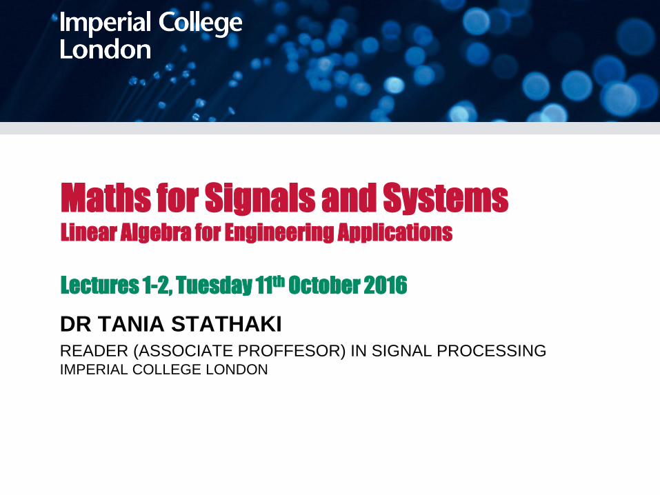
Maths for Signals and Systems Linear Algebra for Engineering Applications
Lectures 1-2, Tuesday 11th October 2016
DR TANIA STATHAKI READER (ASSOCIATE PROFFESOR) IN SIGNAL PROCESSING IMPERIAL COLLEGE LONDON
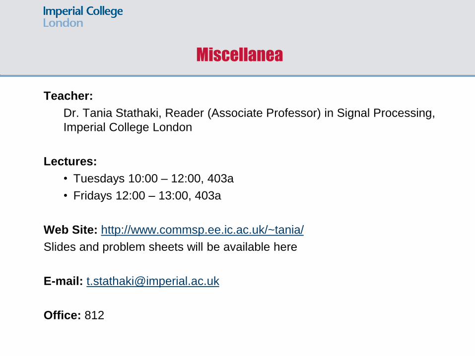
Miscellanea
Teacher:
Dr. Tania Stathaki, Reader (Associate Professor) in Signal Processing,
Imperial College London
Lectures:
• Tuesdays 10:00 – 12:00, 403a
• Fridays 12:00 – 13:00, 403a
Web Site: http://www.commsp.ee.ic.ac.uk/~tania/
Slides and problem sheets will be available here
E-mail: [email protected]
Office: 812
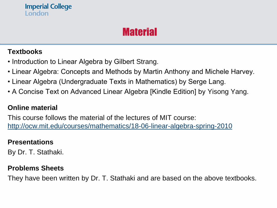
Material
Textbooks
• Introduction to Linear Algebra by Gilbert Strang.
• Linear Algebra: Concepts and Methods by Martin Anthony and Michele Harvey.
• Linear Algebra (Undergraduate Texts in Mathematics) by Serge Lang.
• A Concise Text on Advanced Linear Algebra [Kindle Edition] by Yisong Yang.
Online material
This course follows the material of the lectures of MIT course:
http://ocw.mit.edu/courses/mathematics/18-06-linear-algebra-spring-2010
Presentations
By Dr. T. Stathaki.
Problems Sheets
They have been written by Dr. T. Stathaki and are based on the above textbooks.
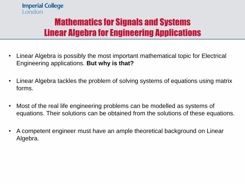
Mathematics for Signals and Systems
Linear Algebra for Engineering Applications
• Linear Algebra is possibly the most important mathematical topic for Electrical
Engineering applications. But why is that?
• Linear Algebra tackles the problem of solving systems of equations using matrix
forms.
• Most of the real life engineering problems can be modelled as systems of
equations. Their solutions can be obtained from the solutions of these equations.
• A competent engineer must have an ample theoretical background on Linear
Algebra.
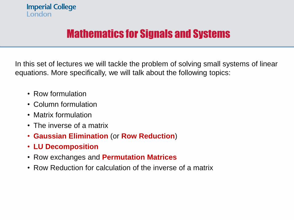
Mathematics for Signals and Systems
In this set of lectures we will tackle the problem of solving small systems of linear
equations. More specifically, we will talk about the following topics:
• Row formulation
• Column formulation
• Matrix formulation
• The inverse of a matrix
• Gaussian Elimination (or Row Reduction)
• LU Decomposition
• Row exchanges and Permutation Matrices
• Row Reduction for calculation of the inverse of a matrix
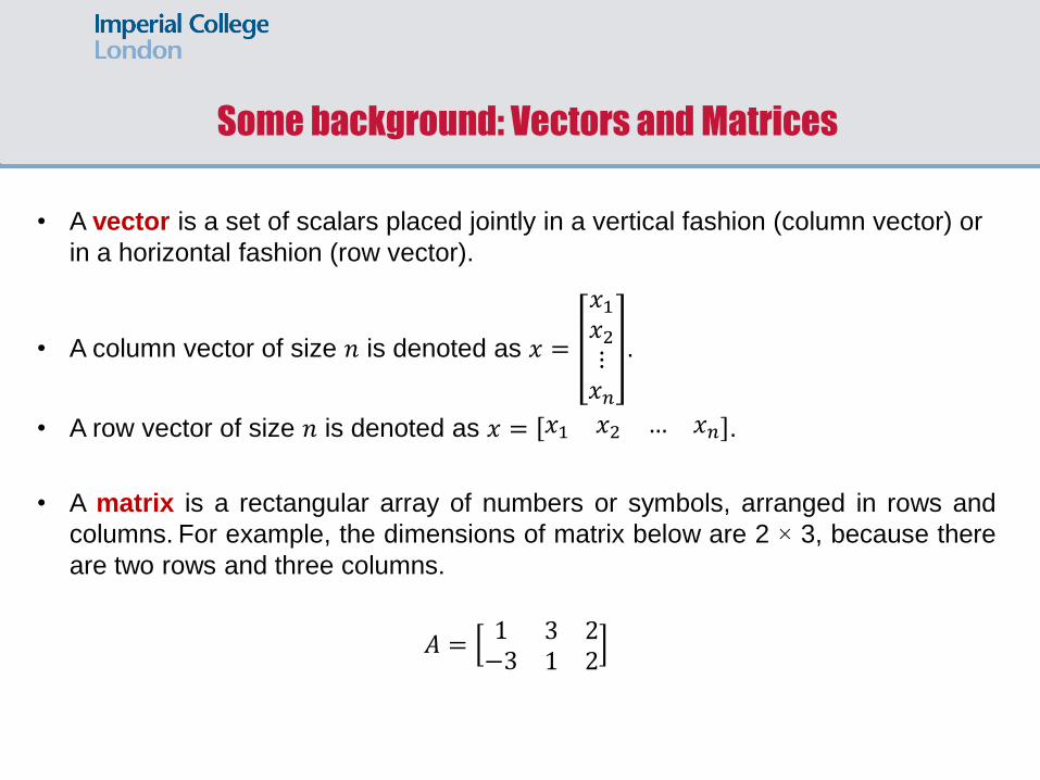
Some background: Vectors and Matrices
• A vector is a set of scalars placed jointly in a vertical fashion (column vector) or
in a horizontal fashion (row vector).
• A column vector of size 𝑛 is denoted as 𝑥 =
𝑥1
𝑥2
⋮𝑥𝑛
.
• A row vector of size 𝑛 is denoted as 𝑥 = 𝑥1 𝑥2 … 𝑥𝑛 .
• A matrix is a rectangular array of numbers or symbols, arranged in rows and
columns. For example, the dimensions of matrix below are 2 × 3, because there
are two rows and three columns.
𝐴 =1−3
31
22
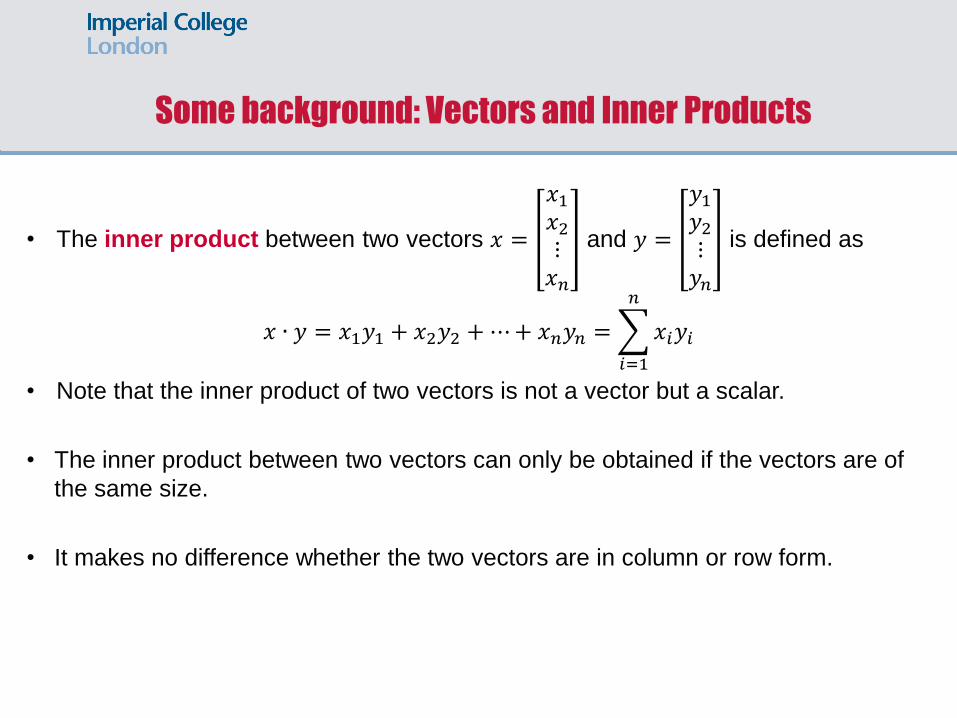
Some background: Vectors and Inner Products
• The inner product between two vectors 𝑥 =
𝑥1
𝑥2
⋮𝑥𝑛
and 𝑦 =
𝑦1
𝑦2
⋮𝑦𝑛
is defined as
𝑥 ∙ 𝑦 = 𝑥1𝑦1 + 𝑥2𝑦2 + ⋯+ 𝑥𝑛𝑦𝑛 = 𝑥𝑖𝑦𝑖
𝑛
𝑖=1
• Note that the inner product of two vectors is not a vector but a scalar.
• The inner product between two vectors can only be obtained if the vectors are of
the same size.
• It makes no difference whether the two vectors are in column or row form.
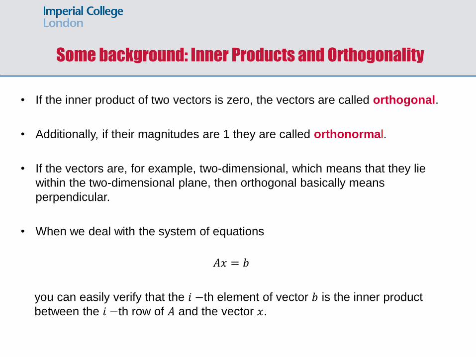
Some background: Inner Products and Orthogonality
• If the inner product of two vectors is zero, the vectors are called orthogonal.
• Additionally, if their magnitudes are 1 they are called orthonormal.
• If the vectors are, for example, two-dimensional, which means that they lie
within the two-dimensional plane, then orthogonal basically means
perpendicular.
• When we deal with the system of equations
𝐴𝑥 = 𝑏
you can easily verify that the 𝑖 −th element of vector 𝑏 is the inner product
between the 𝑖 −th row of 𝐴 and the vector 𝑥.
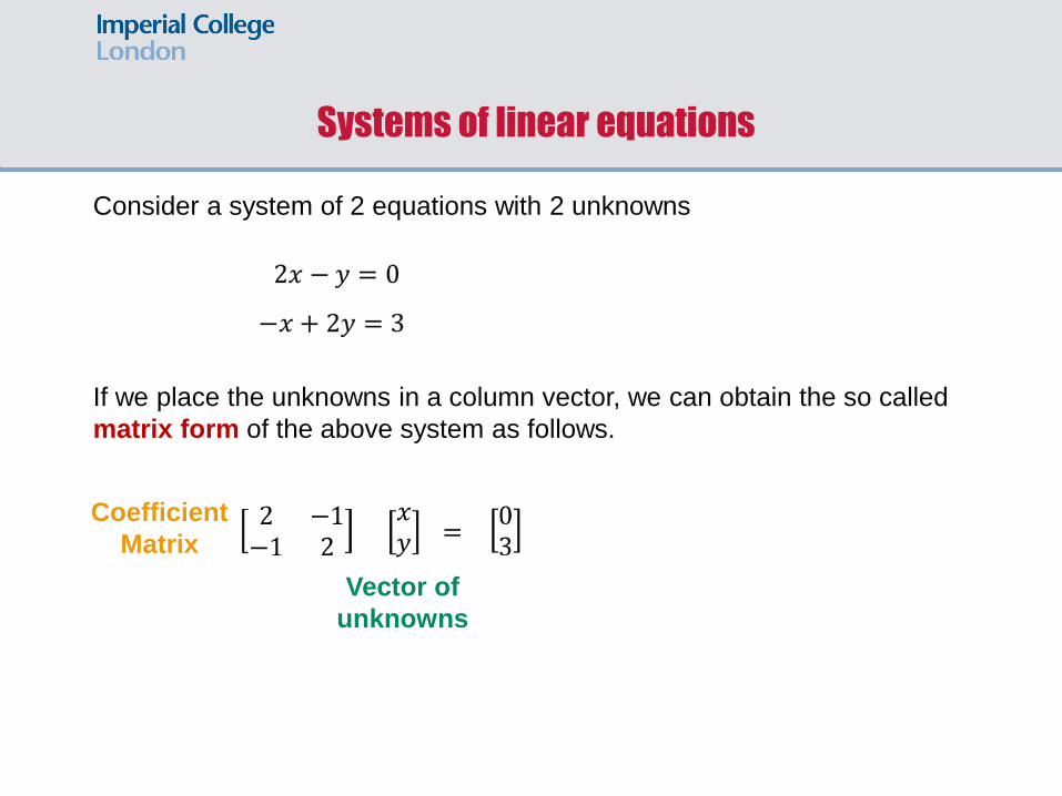
Systems of linear equations
Consider a system of 2 equations with 2 unknowns
If we place the unknowns in a column vector, we can obtain the so called
matrix form of the above system as follows.
Vector of
unknowns
Coefficient
Matrix
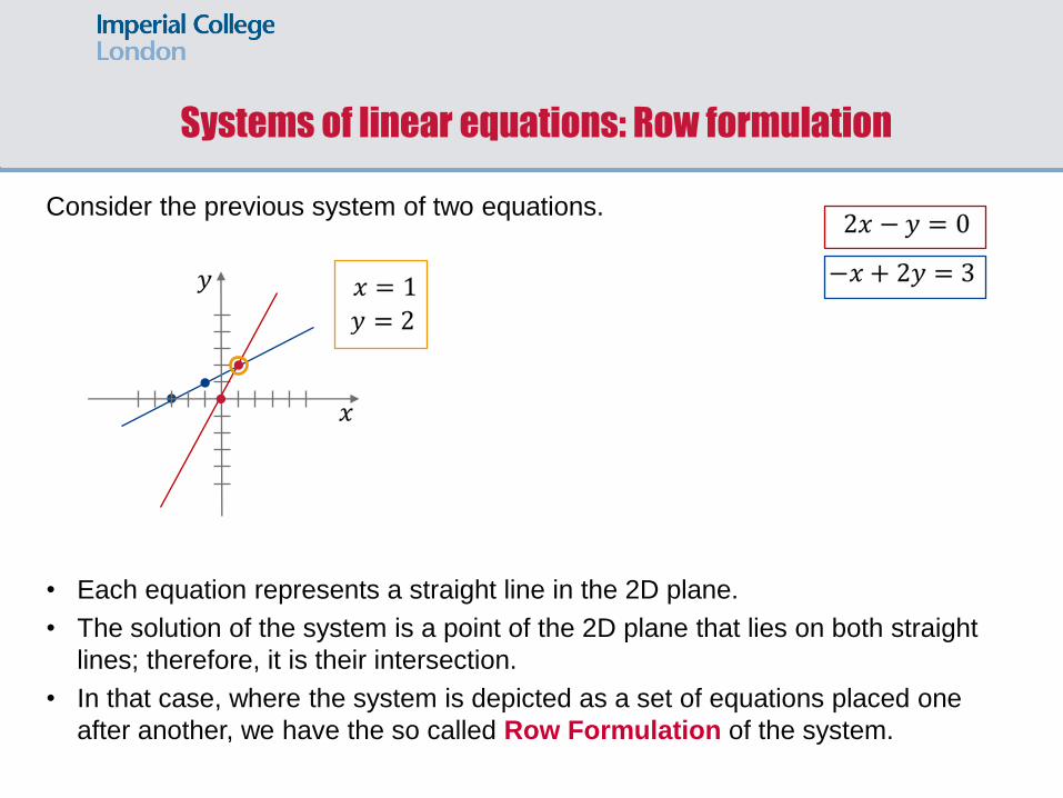
Systems of linear equations: Row formulation
Consider the previous system of two equations.
• Each equation represents a straight line in the 2D plane.
• The solution of the system is a point of the 2D plane that lies on both straight
lines; therefore, it is their intersection.
• In that case, where the system is depicted as a set of equations placed one
after another, we have the so called Row Formulation of the system.
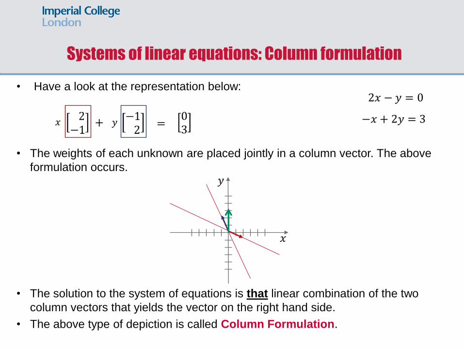
Systems of linear equations: Column formulation
• Have a look at the representation below:
• The weights of each unknown are placed jointly in a column vector. The above
formulation occurs.
• The solution to the system of equations is that linear combination of the two
column vectors that yields the vector on the right hand side.
• The above type of depiction is called Column Formulation.
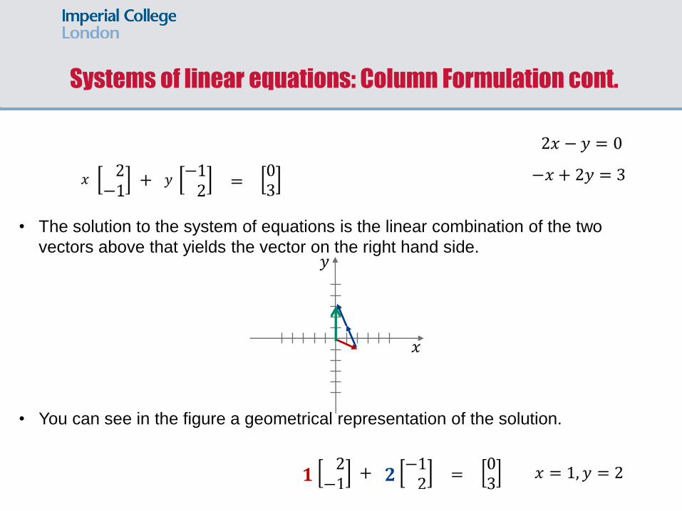
• The solution to the system of equations is the linear combination of the two
vectors above that yields the vector on the right hand side.
• You can see in the figure a geometrical representation of the solution.
Systems of linear equations: Column Formulation cont.
Systems of linear equations: Column Formulation cont.
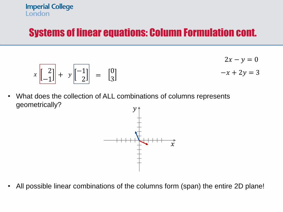
• What does the collection of ALL combinations of columns represents
geometrically?
• All possible linear combinations of the columns form (span) the entire 2D plane!
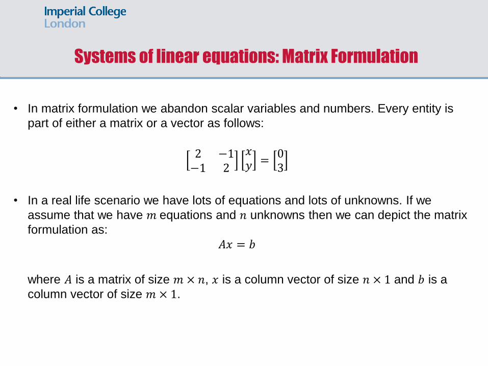
• In matrix formulation we abandon scalar variables and numbers. Every entity is
part of either a matrix or a vector as follows:
2 −1−1 2
𝑥𝑦 =
03
• In a real life scenario we have lots of equations and lots of unknowns. If we
assume that we have 𝑚 equations and 𝑛 unknowns then we can depict the matrix
formulation as:
𝐴𝑥 = 𝑏
where 𝐴 is a matrix of size 𝑚 × 𝑛, 𝑥 is a column vector of size 𝑛 × 1 and 𝑏 is a
column vector of size 𝑚 × 1.
Systems of linear equations: Matrix Formulation
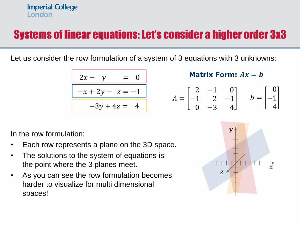
Let us consider the row formulation of a system of 3 equations with 3 unknowns:
In the row formulation:
• Each row represents a plane on the 3D space.
• The solutions to the system of equations is
the point where the 3 planes meet.
• As you can see the row formulation becomes
harder to visualize for multi dimensional
spaces!
Systems of linear equations: Let’s consider a higher order 3x3
Matrix Form: 𝑨𝒙 = 𝒃
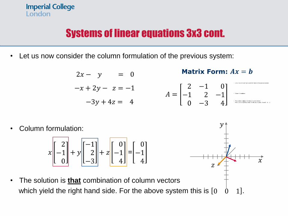
• Let us now consider the column formulation of the previous system:
• Column formulation:
• The solution is that combination of column vectors
which yield the right hand side. For the above system this is 0 0 1 .
Systems of linear equations 3x3 cont.
Matrix Form: 𝑨𝒙 = 𝒃
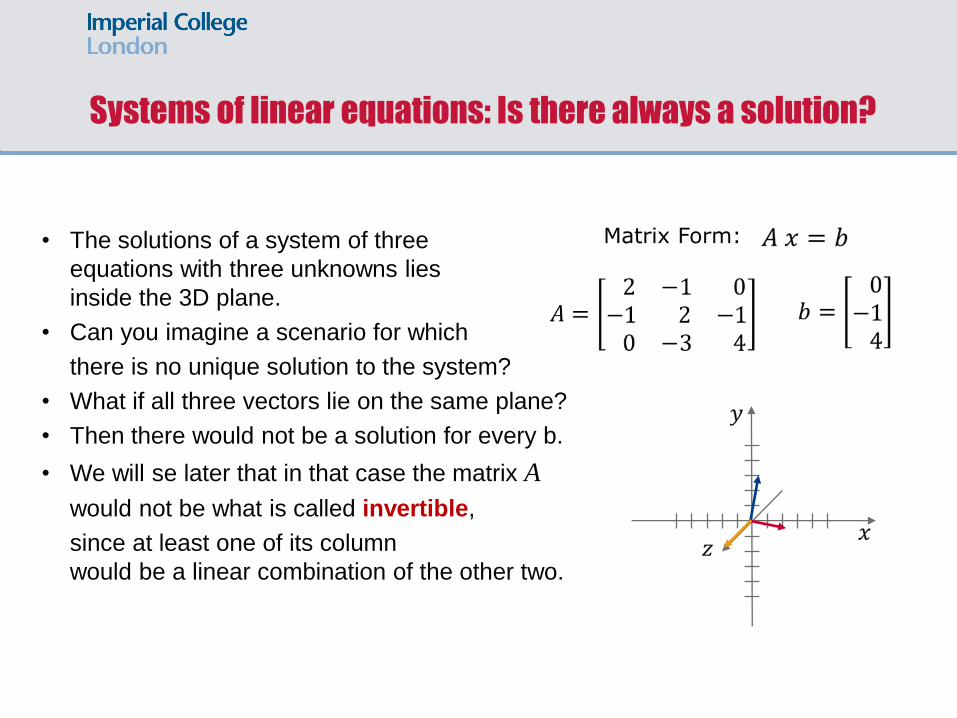
Systems of linear equations: Is there always a solution?
• The solutions of a system of three
equations with three unknowns lies
inside the 3D plane.
• Can you imagine a scenario for which
there is no unique solution to the system?
• What if all three vectors lie on the same plane?
• Then there would not be a solution for every b.
• We will se later that in that case the matrix A
would not be what is called invertible,
since at least one of its column
would be a linear combination of the other two.
Matrix Form:
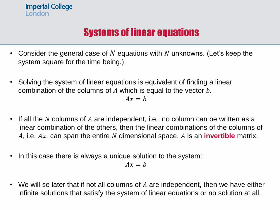
Systems of linear equations
• Consider the general case of 𝑁 equations with 𝑁 unknowns. (Let’s keep the
system square for the time being.)
• Solving the system of linear equations is equivalent of finding a linear
combination of the columns of 𝐴 which is equal to the vector 𝑏.
𝐴𝑥 = 𝑏
• If all the 𝑁 columns of 𝐴 are independent, i.e., no column can be written as a
linear combination of the others, then the linear combinations of the columns of
𝐴, i.e. 𝐴𝑥, can span the entire 𝑁 dimensional space. 𝐴 is an invertible matrix.
• In this case there is always a unique solution to the system:
𝐴𝑥 = 𝑏
• We will se later that if not all columns of 𝐴 are independent, then we have either
infinite solutions that satisfy the system of linear equations or no solution at all.
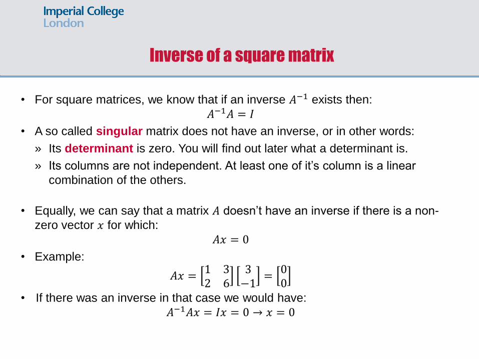
Inverse of a square matrix
• For square matrices, we know that if an inverse 𝐴−1 exists then:
𝐴−1𝐴 = 𝐼
• A so called singular matrix does not have an inverse, or in other words:
» Its determinant is zero. You will find out later what a determinant is.
» Its columns are not independent. At least one of it’s column is a linear
combination of the others.
• Equally, we can say that a matrix 𝐴 doesn’t have an inverse if there is a non-
zero vector 𝑥 for which:
𝐴𝑥 = 0
• Example:
𝐴𝑥 =1 32 6
3−1
=00
• If there was an inverse in that case we would have:
𝐴−1𝐴𝑥 = 𝐼𝑥 = 0 → 𝑥 = 0
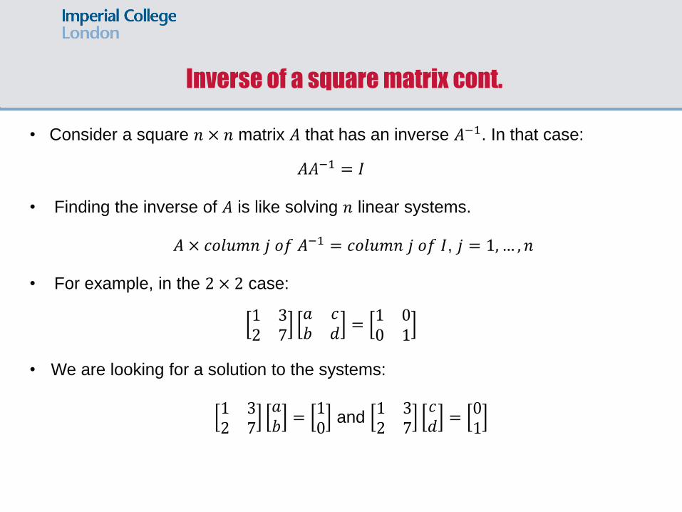
Inverse of a square matrix cont.
• Consider a square 𝑛 × 𝑛 matrix 𝐴 that has an inverse 𝐴−1. In that case:
𝐴𝐴−1 = 𝐼
• Finding the inverse of 𝐴 is like solving 𝑛 linear systems.
𝐴 × 𝑐𝑜𝑙𝑢𝑚𝑛 𝑗 𝑜𝑓 𝐴−1 = 𝑐𝑜𝑙𝑢𝑚𝑛 𝑗 𝑜𝑓 𝐼, 𝑗 = 1, … , 𝑛
• For example, in the 2 × 2 case:
1 32 7
𝑎 𝑐𝑏 𝑑
=1 00 1
• We are looking for a solution to the systems:
1 32 7
𝑎𝑏
=10
and 1 32 7
𝑐𝑑
=01
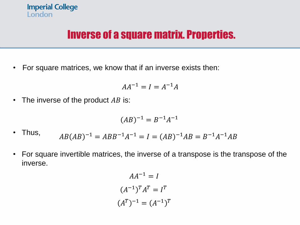
Inverse of a square matrix. Properties.
• For square matrices, we know that if an inverse exists then:
• The inverse of the product 𝐴𝐵 is:
• Thus,
• For square invertible matrices, the inverse of a transpose is the transpose of the
inverse.
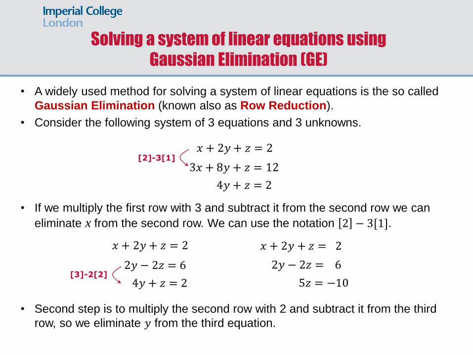
• A widely used method for solving a system of linear equations is the so called
Gaussian Elimination (known also as Row Reduction).
• Consider the following system of 3 equations and 3 unknowns.
• If we multiply the first row with 3 and subtract it from the second row we can
eliminate x from the second row. We can use the notation 2 − 3[1].
• Second step is to multiply the second row with 2 and subtract it from the third
row, so we eliminate 𝑦 from the third equation.
Solving a system of linear equations using
Gaussian Elimination (GE)
[2]-3[1]
[3]-2[2]
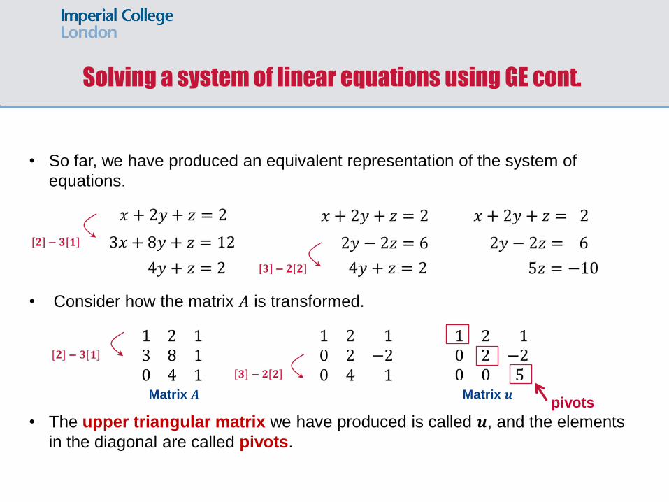
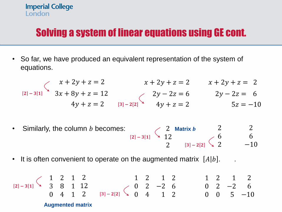
• So far, we have produced an equivalent representation of the system of
equations.
• Consider how the matrix 𝐴 is transformed.
• The upper triangular matrix we have produced is called 𝒖, and the elements
in the diagonal are called pivots.
Matrix 𝑨
Solving a system of linear equations using GE cont.
Matrix 𝒖 pivots
• So far, we have produced an equivalent representation of the system of
equations.
• Similarly, the column 𝑏 becomes:
• It is often convenient to operate on the augmented matrix 𝐴 𝑏 . .
Matrix 𝒃
Solving a system of linear equations using GE cont.
Augmented matrix
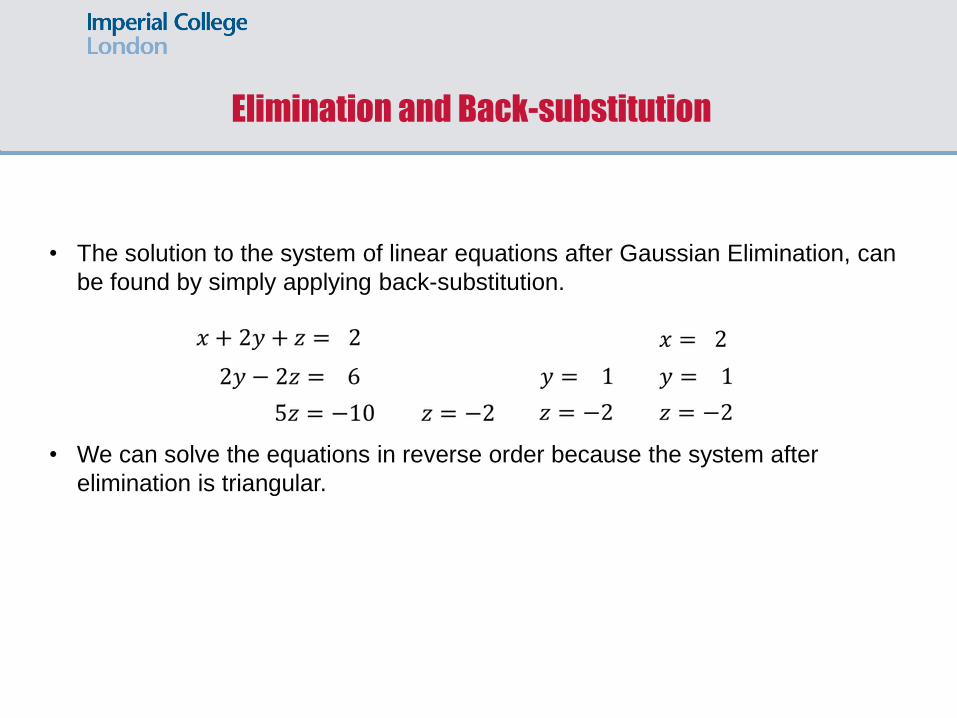
• The solution to the system of linear equations after Gaussian Elimination, can
be found by simply applying back-substitution.
• We can solve the equations in reverse order because the system after
elimination is triangular.
Elimination and Back-substitution
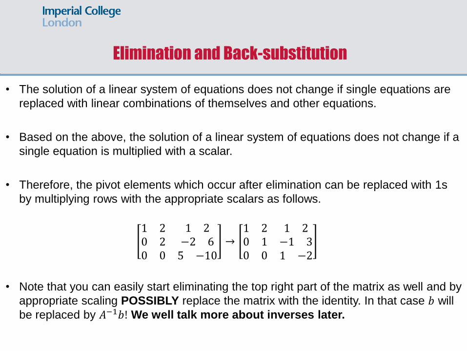
• The solution of a linear system of equations does not change if single equations are
replaced with linear combinations of themselves and other equations.
• Based on the above, the solution of a linear system of equations does not change if a
single equation is multiplied with a scalar.
• Therefore, the pivot elements which occur after elimination can be replaced with 1s
by multiplying rows with the appropriate scalars as follows.
1 20 20 0
1 2−2 65 −10
→1 20 10 0
1 2−1 31 −2
• Note that you can easily start eliminating the top right part of the matrix as well and by
appropriate scaling POSSIBLY replace the matrix with the identity. In that case 𝑏 will
be replaced by 𝐴−1𝑏! We well talk more about inverses later.
Elimination and Back-substitution
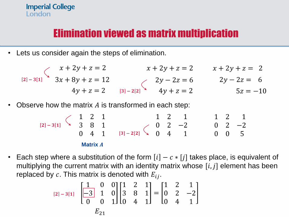
• Lets us consider again the steps of elimination.
• Observe how the matrix 𝐴 is transformed in each step:
• Each step where a substitution of the form 𝑖 − 𝑐 ∗ [𝑗] takes place, is equivalent of
multiplying the current matrix with an identity matrix whose [𝑖, 𝑗] element has been
replaced by 𝑐. This matrix is denoted with 𝐸𝑖𝑗.
Elimination viewed as matrix multiplication
Matrix 𝑨
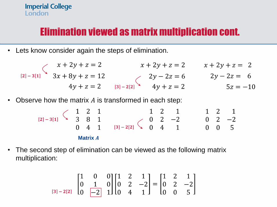
• Lets know consider again the steps of elimination.
• Observe how the matrix 𝐴 is transformed in each step:
• The second step of elimination can be viewed as the following matrix
multiplication:
Elimination viewed as matrix multiplication cont.
Matrix 𝑨
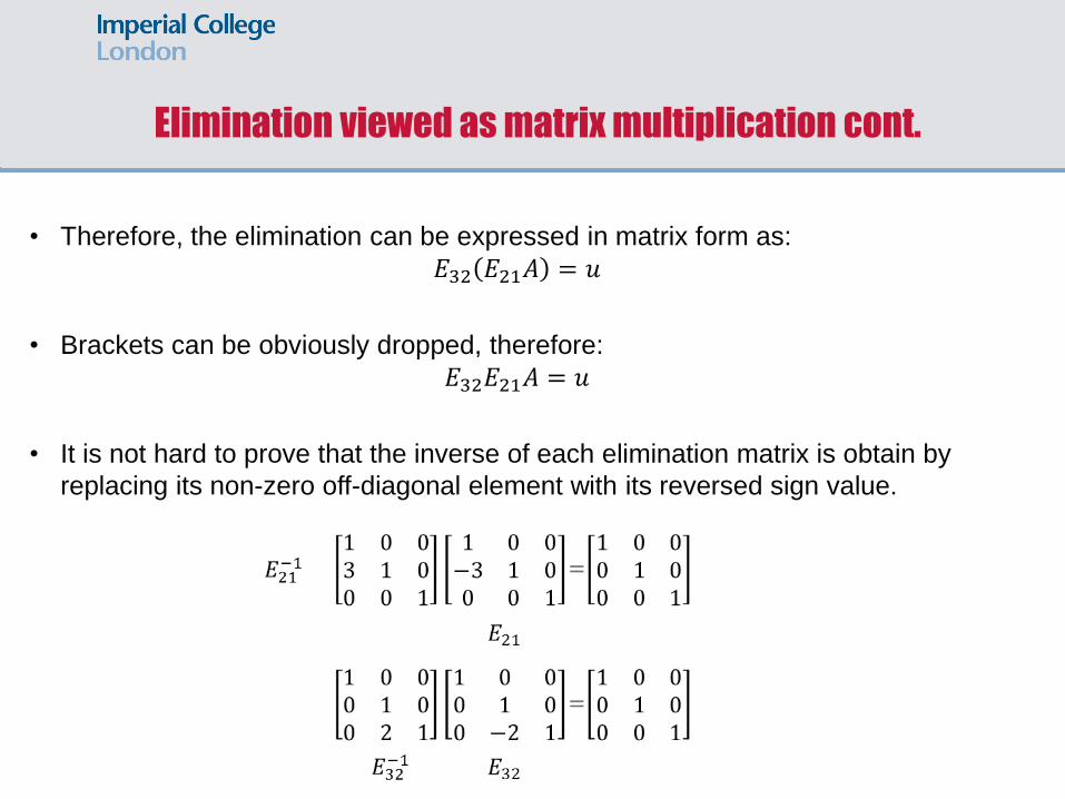
• Therefore, the elimination can be expressed in matrix form as:
𝐸32 𝐸21𝐴 = 𝑢
• Brackets can be obviously dropped, therefore:
𝐸32𝐸21𝐴 = 𝑢
• It is not hard to prove that the inverse of each elimination matrix is obtain by
replacing its non-zero off-diagonal element with its reversed sign value.
Elimination viewed as matrix multiplication cont.
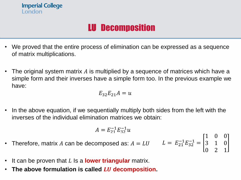
• We proved that the entire process of elimination can be expressed as a sequence
of matrix multiplications.
• The original system matrix 𝐴 is multiplied by a sequence of matrices which have a
simple form and their inverses have a simple form too. In the previous example we
have:
𝐸32𝐸21𝐴 = 𝑢
• In the above equation, if we sequentially multiply both sides from the left with the
inverses of the individual elimination matrices we obtain:
• Therefore, matrix 𝐴 can be decomposed as: 𝐴 = 𝐿𝑈
• It can be proven that 𝐿 Is a lower triangular matrix.
• The above formulation is called 𝑳𝑼 decomposition.
LU Decomposition
LU Decomposition in the general case
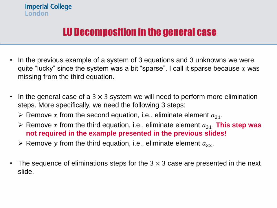
• In the previous example of a system of 3 equations and 3 unknowns we were
quite “lucky” since the system was a bit “sparse”. I call it sparse because 𝑥 was
missing from the third equation.
• In the general case of a 3 × 3 system we will need to perform more elimination
steps. More specifically, we need the following 3 steps:
Remove 𝑥 from the second equation, i.e., eliminate element 𝑎21.
Remove 𝑥 from the third equation, i.e., eliminate element 𝑎31. This step was
not required in the example presented in the previous slides!
Remove 𝑦 from the third equation, i.e., eliminate element 𝑎32.
• The sequence of eliminations steps for the 3 × 3 case are presented in the next
slide.
LU Decomposition in the general case
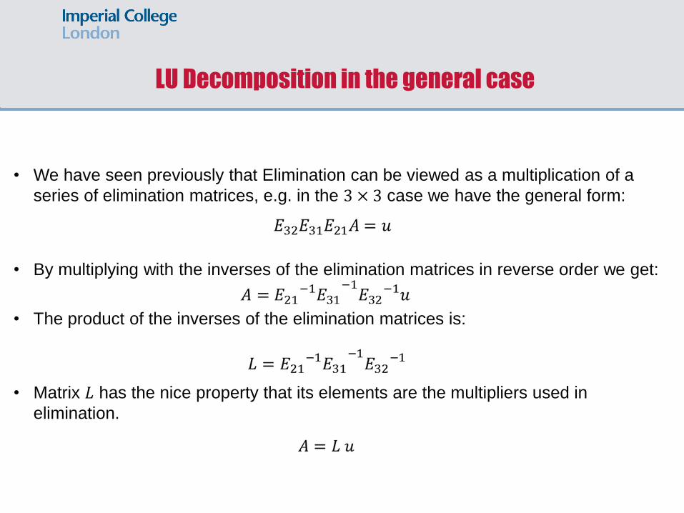
• We have seen previously that Elimination can be viewed as a multiplication of a
series of elimination matrices, e.g. in the 3 × 3 case we have the general form:
• By multiplying with the inverses of the elimination matrices in reverse order we get:
• The product of the inverses of the elimination matrices is:
• Matrix 𝐿 has the nice property that its elements are the multipliers used in
elimination.

LU Decomposition with row exchanges. Permutation. • Often in order to create the upper triangular matrix 𝑢 through elimination we
must reorder the rows of matrix 𝐴 first (why?)
• In the general case where row exchanges are required, for any invertible matrix
𝐴, we have:
𝑃𝐴 = 𝐿𝑢
• 𝑃 is a permutation matrix. This arises from the identity matrix if we reorder the
rows.
• A permutation matrix encodes row exchanges in Gaussian elimination.
• Row exchanges are required when we have a zero in a pivot position.
• For example the following permutation matrix exchanges rows 1 and 2 to get a
non zero in the first pivot position
• As with any orthogonal matrix, for permutation matrices we have 𝑷−𝟏 = 𝑷𝑻!
Calculation of the inverse of a matrix
using row reduction
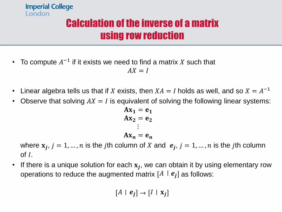
• To compute 𝐴−1 if it exists we need to find a matrix 𝑋 such that
𝐴𝑋 = 𝐼
• Linear algebra tells us that if 𝑋 exists, then 𝑋𝐴 = 𝐼 holds as well, and so 𝑋 = 𝐴−1
• Observe that solving 𝐴𝑋 = 𝐼 is equivalent of solving the following linear systems:
𝐀𝐱𝟏 = 𝐞𝟏
𝐀𝐱𝟐 = 𝐞𝟐
⋮ 𝐀𝐱𝒏 = 𝐞𝒏
where 𝐱𝒋, 𝑗 = 1,… , 𝑛 is the 𝑗th column of 𝑋 and 𝒆𝒋, 𝑗 = 1,… , 𝑛 is the 𝑗th column
of 𝐼.
• If there is a unique solution for each 𝐱𝒋, we can obtain it by using elementary row
operations to reduce the augmented matrix 𝐴 𝒆𝒋 as follows:
𝐴 𝒆𝒋 → 𝐼 𝐱𝒋
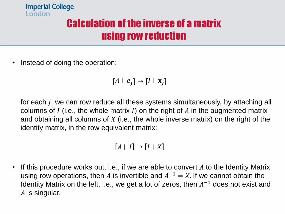
• Instead of doing the operation:
𝐴 𝒆𝒋 → 𝐼 𝐱𝒋
for each 𝑗, we can row reduce all these systems simultaneously, by attaching all
columns of 𝐼 (i.e., the whole matrix 𝐼) on the right of 𝐴 in the augmented matrix
and obtaining all columns of 𝑋 (i.e., the whole inverse matrix) on the right of the
identity matrix, in the row equivalent matrix:
𝐴 𝐼 → 𝐼 𝑋
• If this procedure works out, i.e., if we are able to convert 𝐴 to the Identity Matrix
using row operations, then 𝐴 is invertible and 𝐴−1 = 𝑋. If we cannot obtain the
Identity Matrix on the left, i.e., we get a lot of zeros, then 𝐴−1 does not exist and
𝐴 is singular.
Calculation of the inverse of a matrix
using row reduction
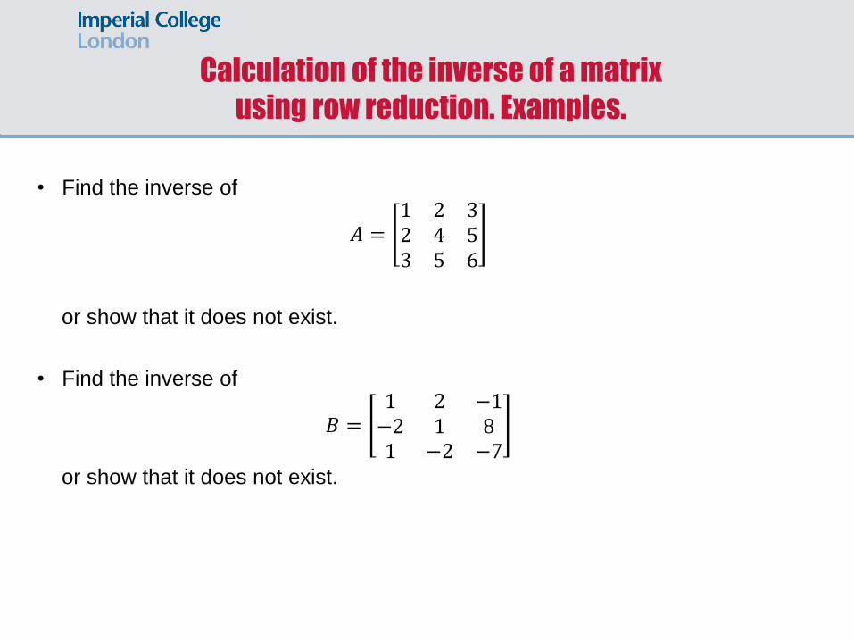
• Find the inverse of
𝐴 =1 2 32 4 53 5 6
or show that it does not exist.
• Find the inverse of
𝐵 =1 2 −1−2 1 81 −2 −7
or show that it does not exist.
Calculation of the inverse of a matrix
using row reduction. Examples.
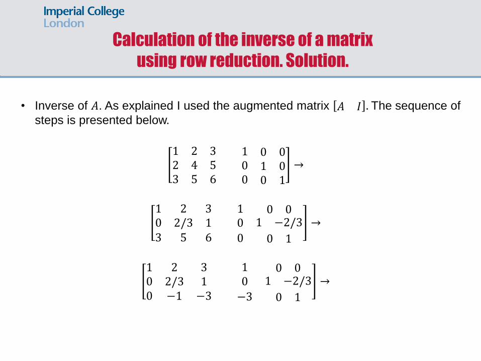
• Inverse of 𝐴. As explained I used the augmented matrix 𝐴 𝐼 . The sequence of
steps is presented below.
1 2 32 4 53 5 6
1 0 00 1 00 0 1
→
1 2 30 2/3 13 5 6
1 0 00 1 −2/3
0 0 1
→
1 2 30 2/3 10 −1 −3
1 0 00 1 −2/3
−3 0 1
→
Calculation of the inverse of a matrix
using row reduction. Solution.
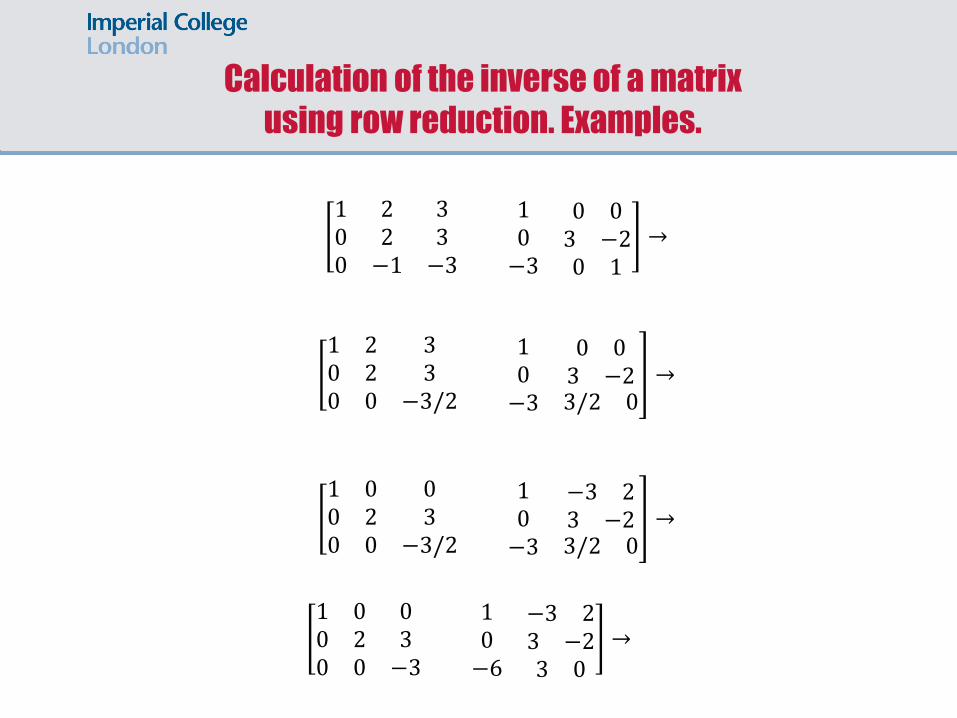
1 2 30 2 30 −1 −3
1 0 00 3 −2−3 0 1
→
1 2 30 2 30 0 −3/2
1 0 00 3 −2−3 3/2 0
→
1 0 00 2 30 0 −3/2
1 −3 20 3 −2−3 3/2 0
→
1 0 00 2 30 0 −3
1 −3 20 3 −2−6 3 0
→
Calculation of the inverse of a matrix
using row reduction. Examples.
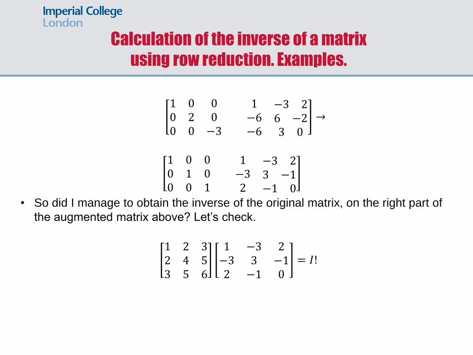
1 0 00 2 00 0 −3
1 −3 2−6 6 −2−6 3 0
→
1 0 00 1 00 0 1
1 −3 2−3 3 −12 −1 0
• So did I manage to obtain the inverse of the original matrix, on the right part of
the augmented matrix above? Let’s check.
1 2 32 4 53 5 6
1 −3 2−3 3 −12 −1 0
= 𝐼!
Calculation of the inverse of a matrix
using row reduction. Examples.
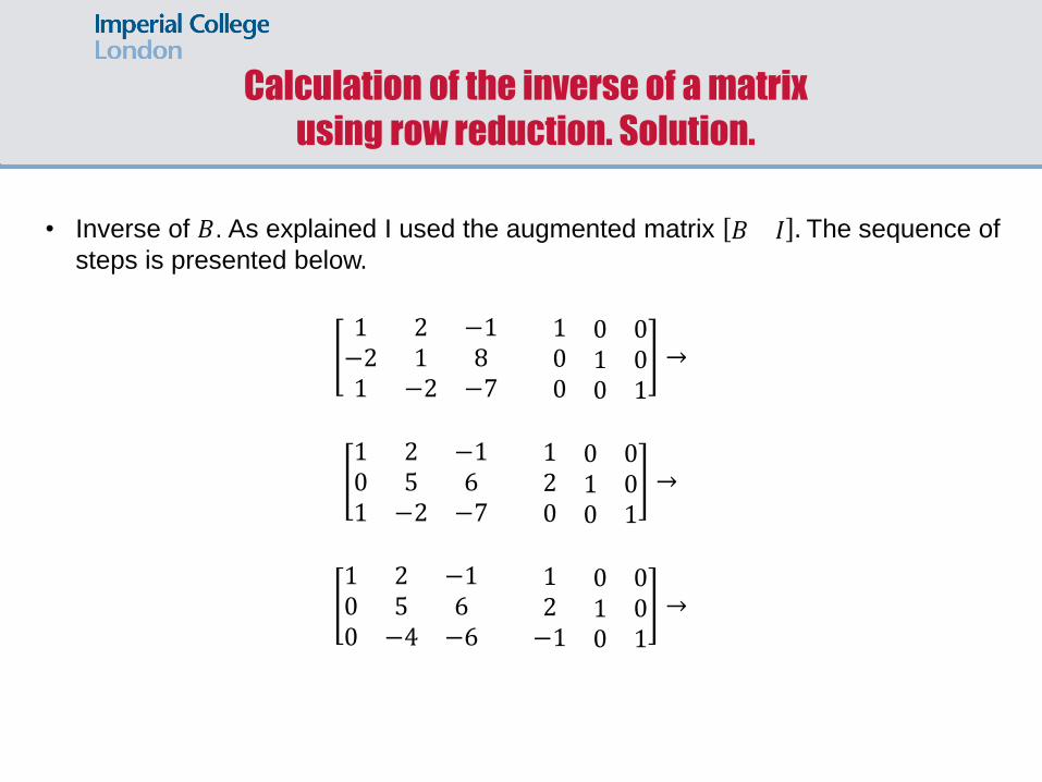
• Inverse of 𝐵. As explained I used the augmented matrix 𝐵 𝐼 . The sequence of
steps is presented below.
1 2 −1−2 1 81 −2 −7
1 0 00 1 00 0 1
→
1 2 −10 5 61 −2 −7
1 0 02 1 00 0 1
→
1 2 −10 5 60 −4 −6
1 0 02 1 0−1 0 1
→
Calculation of the inverse of a matrix
using row reduction. Solution.
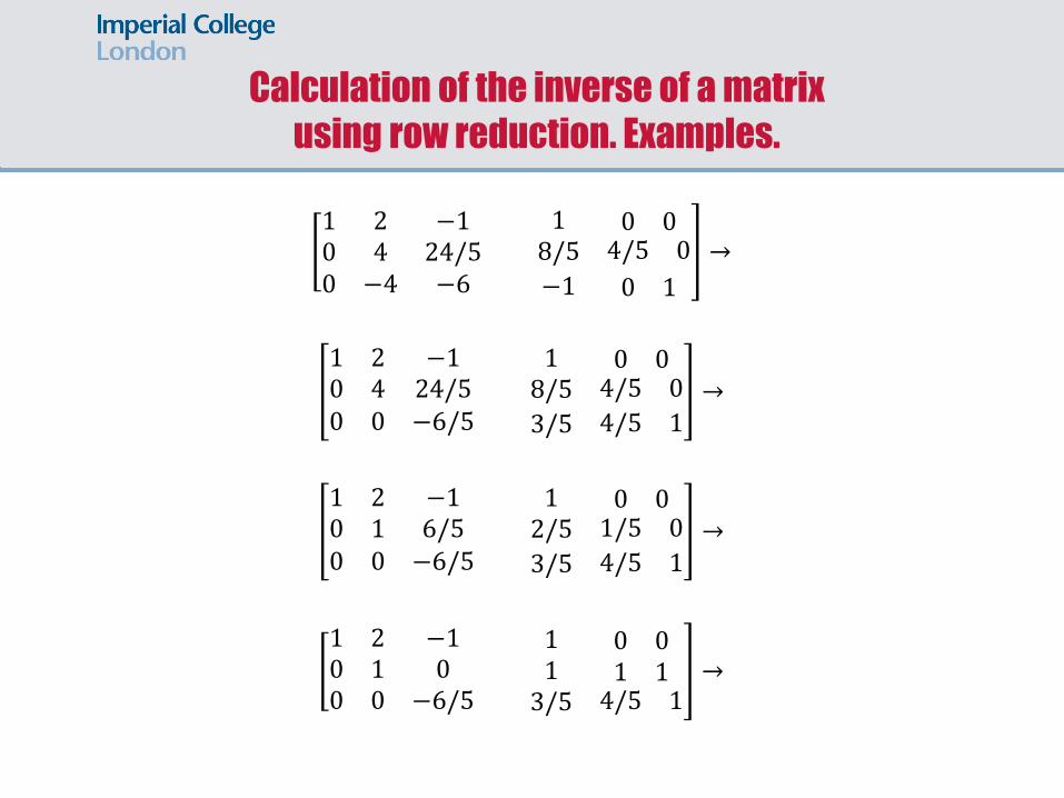
1 2 −10 4 24/50 −4 −6
1 0 08/5 4/5 0
−1 0 1
→
1 2 −10 4 24/50 0 −6/5
1 0 08/5 4/5 0
3/5 4/5 1 →
1 2 −10 1 6/50 0 −6/5
1 0 02/5 1/5 0
3/5 4/5 1 →
1 2 −10 1 00 0 −6/5
1 0 01 1 1
3/5 4/5 1 →
Calculation of the inverse of a matrix
using row reduction. Examples.
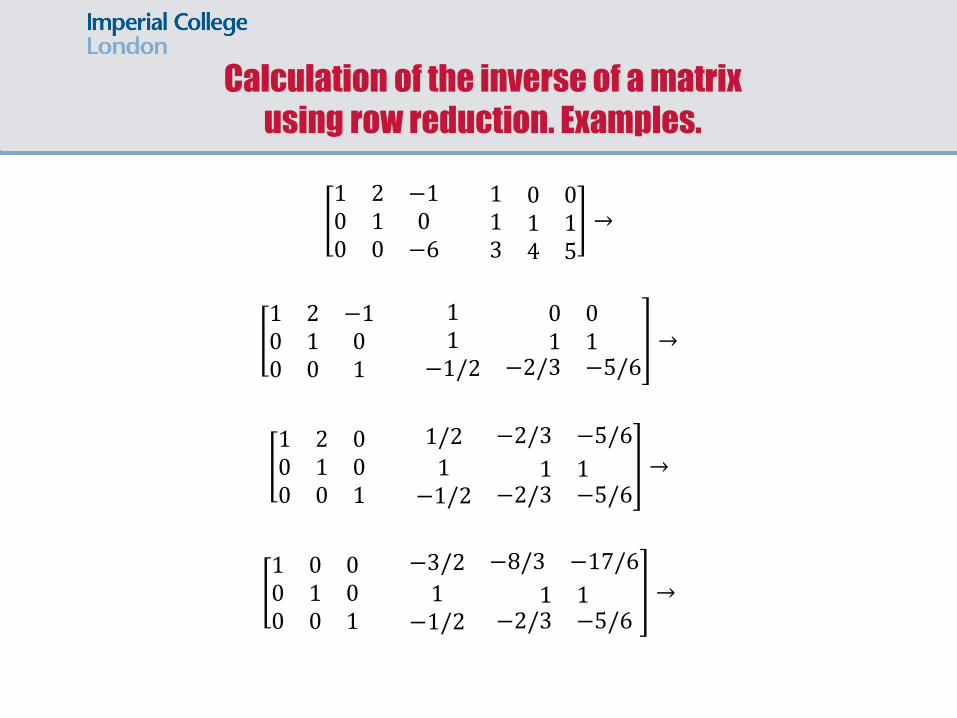
1 2 −10 1 00 0 −6
1 0 01 1 13 4 5
→
1 2 −10 1 00 0 1
1 0 01 1 1
−1/2 −2/3 −5/6 →
1 2 00 1 00 0 1
1/2 −2/3 −5/6
1 1 1−1/2 −2/3 −5/6
→
1 0 00 1 00 0 1
−3/2 −8/3 −17/6
1 1 1−1/2 −2/3 −5/6
→
Calculation of the inverse of a matrix
using row reduction. Examples.
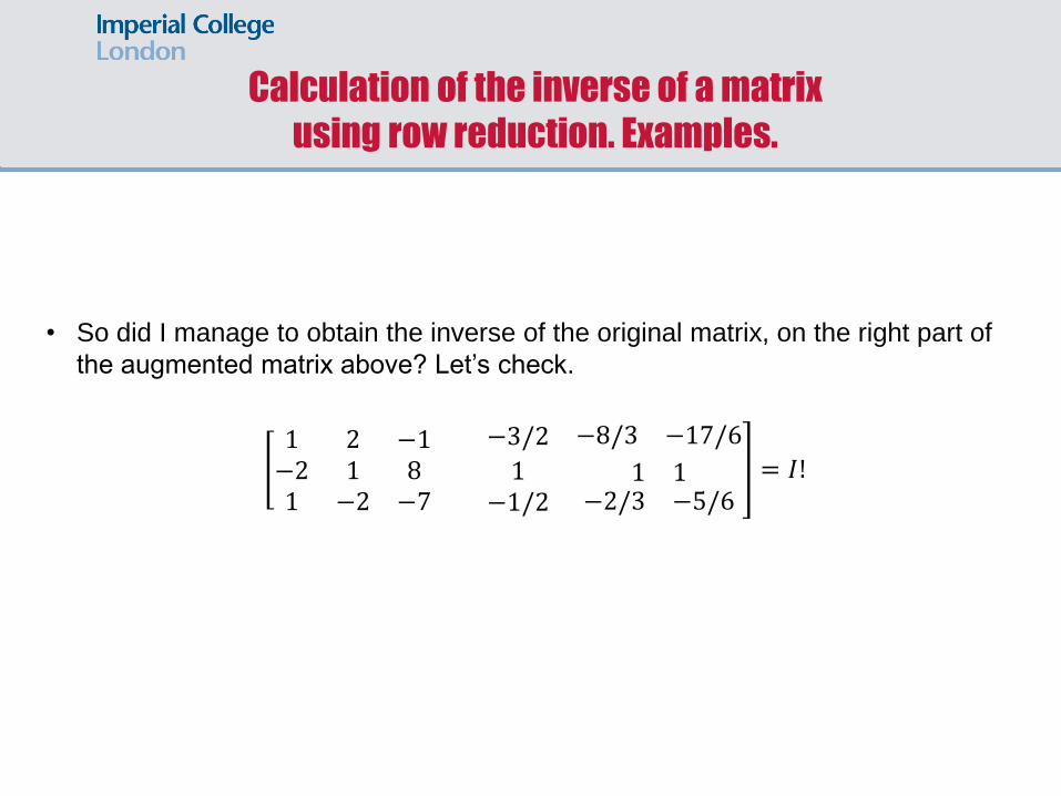
• So did I manage to obtain the inverse of the original matrix, on the right part of
the augmented matrix above? Let’s check.
1 2 −1−2 1 81 −2 −7
−3/2 −8/3 −17/6
1 1 1−1/2 −2/3 −5/6
= 𝐼!
Calculation of the inverse of a matrix
using row reduction. Examples.