Matrix Algebra for OLS Estimator

1

Big Picture

• Matrix algebra can produce compact notation.

• Some packages such as Matlab are matrix-oriented.

• Excel spreadsheet is just a matrix.

2

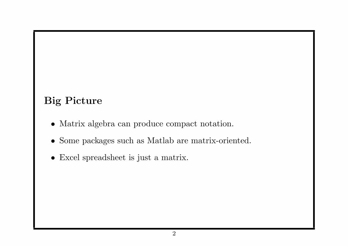
Dependent Variable

• Suppose the sample consists of n observations.

• The dependent variable is denoted as an n× 1 (column) vector

Y =

y1

y2...

yn

• The subscript indexes the observation.

• We use boldface for vector and matrix.

3

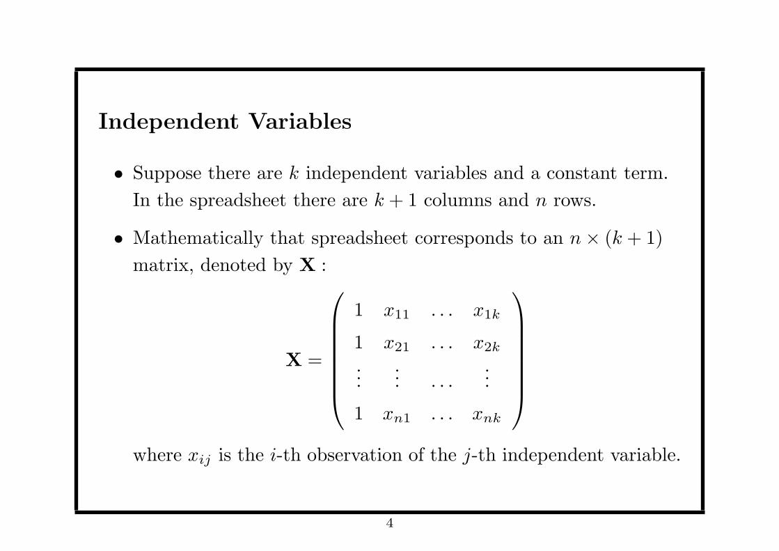
Independent Variables

• Suppose there are k independent variables and a constant term.

In the spreadsheet there are k + 1 columns and n rows.

• Mathematically that spreadsheet corresponds to an n× (k + 1)

matrix, denoted by X :

X =

1 x11 . . . x1k

1 x21 . . . x2k

...... . . .

...

1 xn1 . . . xnk

where xij is the i-th observation of the j-th independent variable.

4

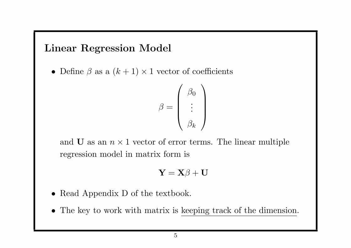
Linear Regression Model

• Define β as a (k + 1)× 1 vector of coefficients

β =

β0

...

βk

and U as an n× 1 vector of error terms. The linear multiple

regression model in matrix form is

Y = Xβ +U

• Read Appendix D of the textbook.

• The key to work with matrix is keeping track of the dimension.

5

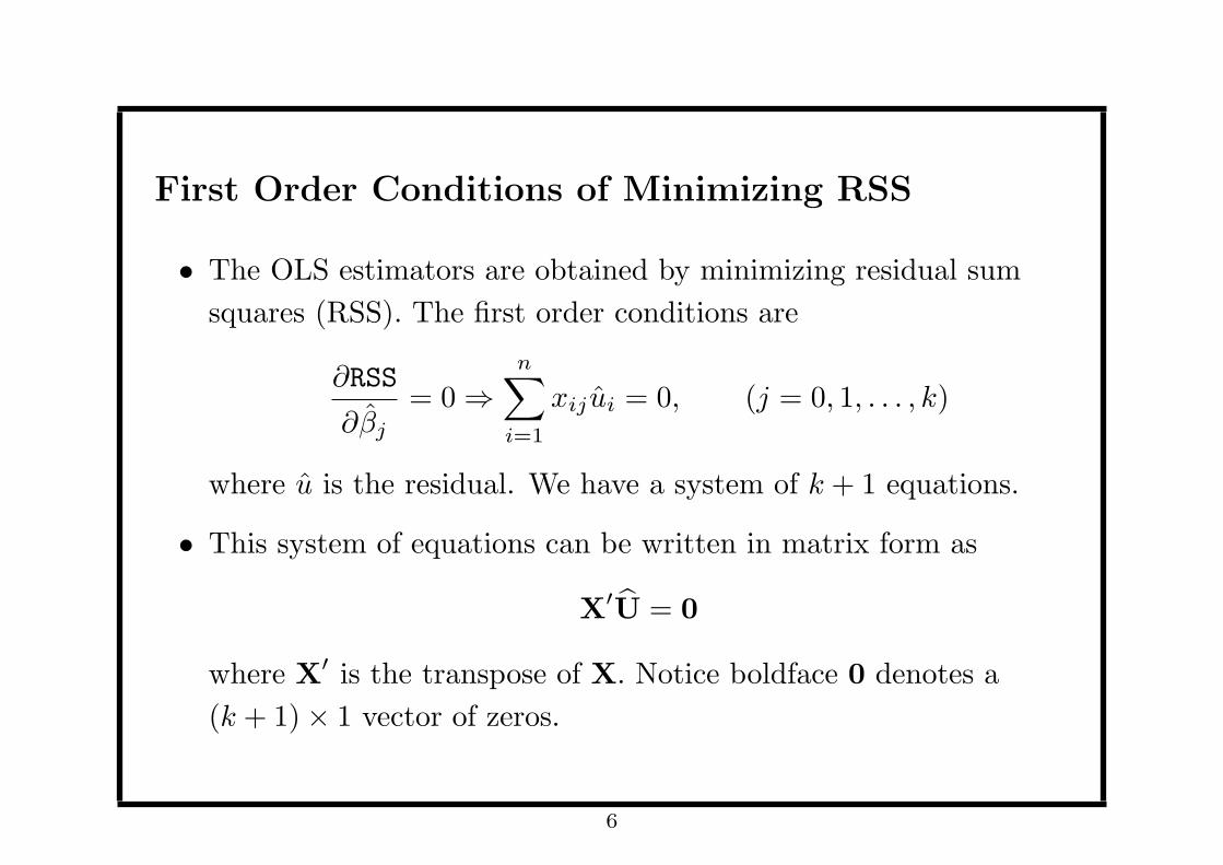
First Order Conditions of Minimizing RSS

• The OLS estimators are obtained by minimizing residual sum

squares (RSS). The first order conditions are

∂RSS

∂βj

= 0 ⇒n∑

i=1

xij ui = 0, (j = 0, 1, . . . , k)

where u is the residual. We have a system of k + 1 equations.

• This system of equations can be written in matrix form as

X′U = 0

where X′ is the transpose of X. Notice boldface 0 denotes a

(k + 1)× 1 vector of zeros.

6

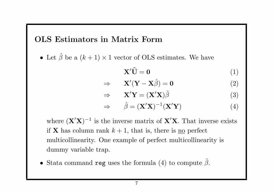
OLS Estimators in Matrix Form

• Let β be a (k + 1)× 1 vector of OLS estimates. We have

X′U = 0 (1)

⇒ X′(Y−Xβ) = 0 (2)

⇒ X′Y = (X′X)β (3)

⇒ β = (X′X)−1(X′Y) (4)

where (X′X)−1 is the inverse matrix of X′X. That inverse exists

if X has column rank k + 1, that is, there is no perfect

multicollinearity. One example of perfect multicollinearity is

dummy variable trap.

• Stata command reg uses the formula (4) to compute β.

7

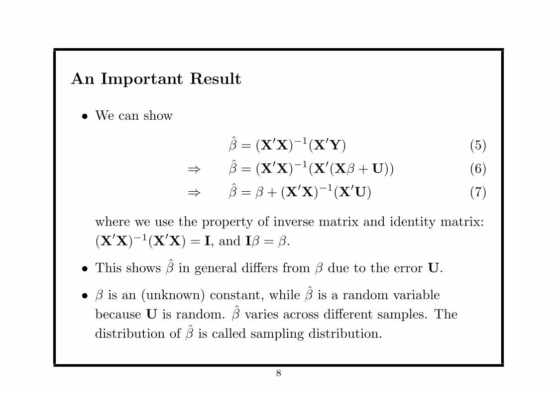
An Important Result

• We can show

β = (X′X)−1(X′Y) (5)

⇒ β = (X′X)−1(X′(Xβ +U)) (6)

⇒ β = β + (X′X)−1(X′U) (7)

where we use the property of inverse matrix and identity matrix:

(X′X)−1(X′X) = I, and Iβ = β.

• This shows β in general differs from β due to the error U.

• β is an (unknown) constant, while β is a random variable

because U is random. β varies across different samples. The

distribution of β is called sampling distribution.

8

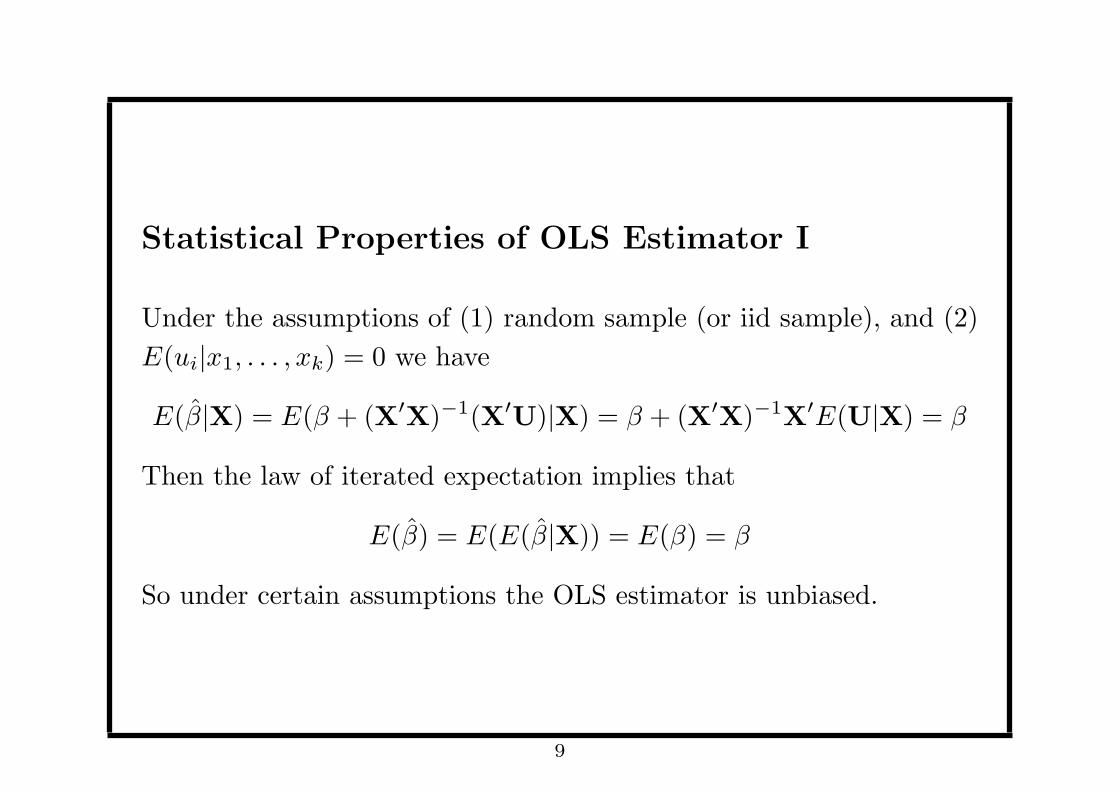
Statistical Properties of OLS Estimator I

Under the assumptions of (1) random sample (or iid sample), and (2)

E(ui|x1, . . . , xk) = 0 we have

E(β|X) = E(β + (X′X)−1(X′U)|X) = β + (X′X)−1X′E(U|X) = β

Then the law of iterated expectation implies that

E(β) = E(E(β|X)) = E(β) = β

So under certain assumptions the OLS estimator is unbiased.

9

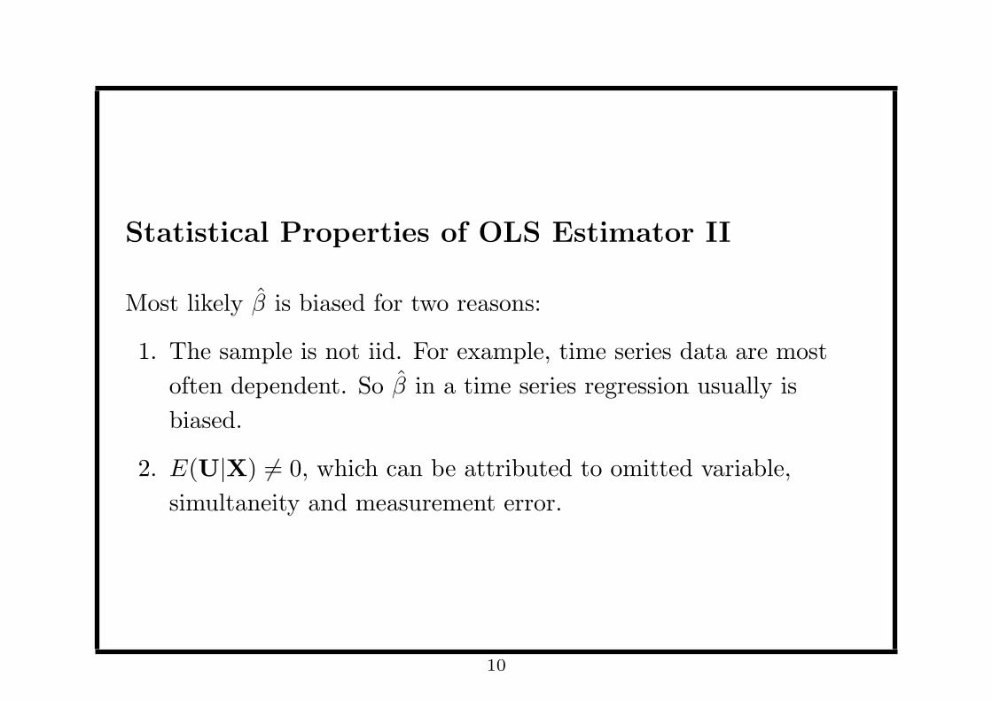
Statistical Properties of OLS Estimator II

Most likely β is biased for two reasons:

1. The sample is not iid. For example, time series data are most

often dependent. So β in a time series regression usually is

biased.

2. E(U|X) = 0, which can be attributed to omitted variable,

simultaneity and measurement error.

10

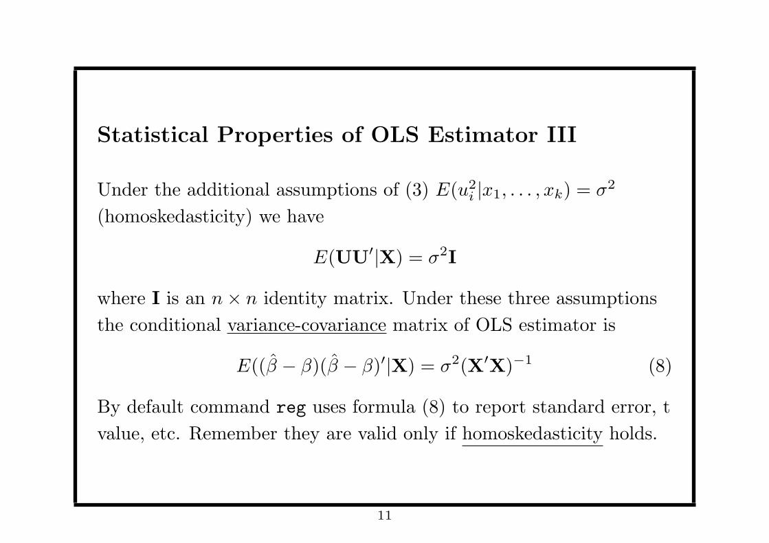
Statistical Properties of OLS Estimator III

Under the additional assumptions of (3) E(u2i |x1, . . . , xk) = σ2

(homoskedasticity) we have

E(UU′|X) = σ2I

where I is an n× n identity matrix. Under these three assumptions

the conditional variance-covariance matrix of OLS estimator is

E((β − β)(β − β)′|X) = σ2(X′X)−1 (8)

By default command reg uses formula (8) to report standard error, t

value, etc. Remember they are valid only if homoskedasticity holds.

11

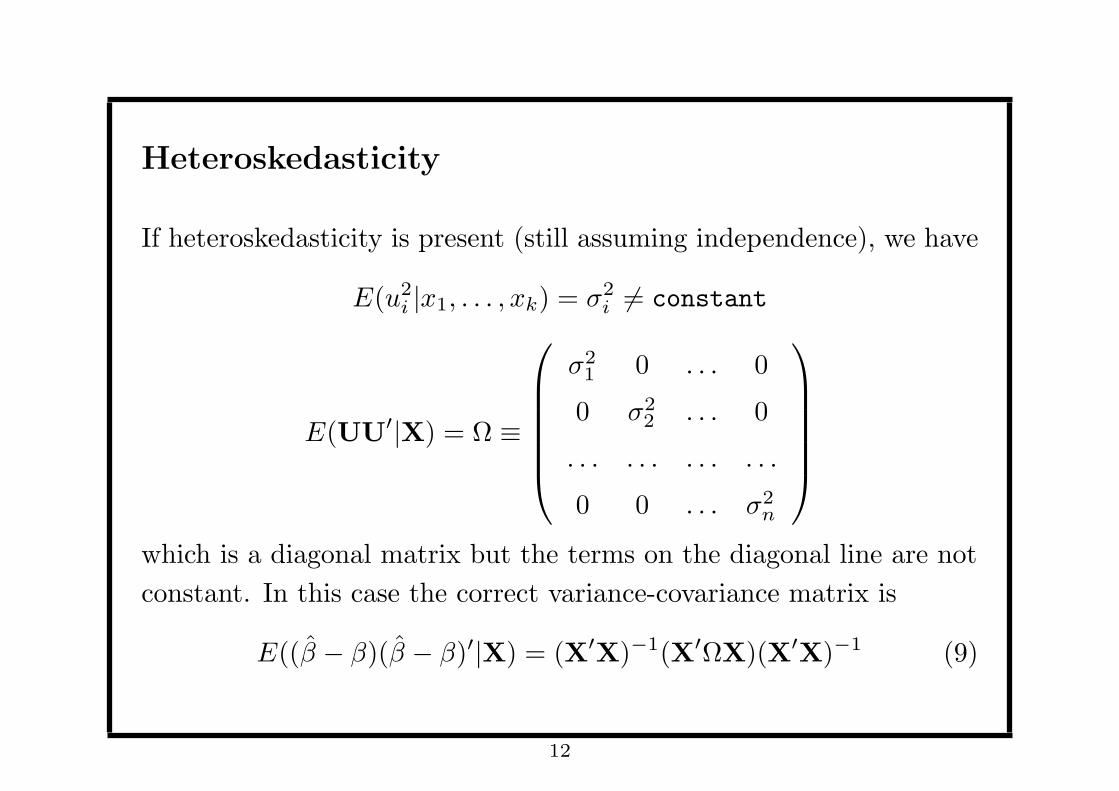
Heteroskedasticity

If heteroskedasticity is present (still assuming independence), we have

E(u2i |x1, . . . , xk) = σ2

i = constant

E(UU′|X) = Ω ≡

σ21 0 . . . 0

0 σ22 . . . 0

. . . . . . . . . . . .

0 0 . . . σ2n

which is a diagonal matrix but the terms on the diagonal line are not

constant. In this case the correct variance-covariance matrix is

E((β − β)(β − β)′|X) = (X′X)−1(X′ΩX)(X′X)−1 (9)

12

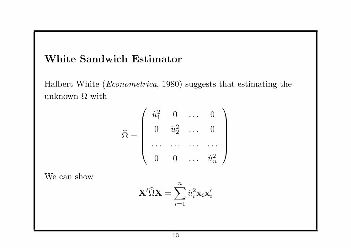
White Sandwich Estimator

Halbert White (Econometrica, 1980) suggests that estimating the

unknown Ω with

Ω =

u21 0 . . . 0

0 u22 . . . 0

. . . . . . . . . . . .

0 0 . . . u2n

We can show

X′ΩX =n∑

i=1

u2ixix

′i

13

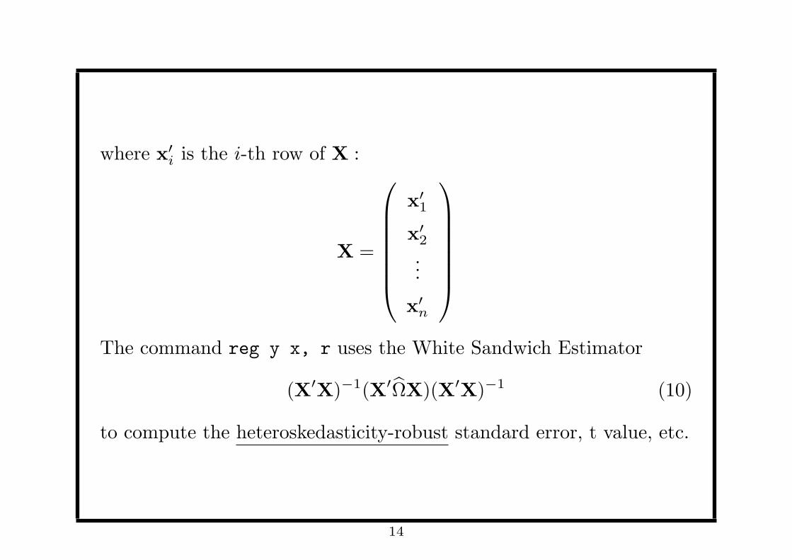
where x′i is the i-th row of X :

X =

x′1

x′2

...

x′n

The command reg y x, r uses the White Sandwich Estimator

(X′X)−1(X′ΩX)(X′X)−1 (10)

to compute the heteroskedasticity-robust standard error, t value, etc.

14

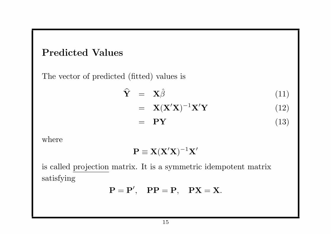
Predicted Values

The vector of predicted (fitted) values is

Y = Xβ (11)

= X(X′X)−1X′Y (12)

= PY (13)

where

P ≡ X(X′X)−1X′

is called projection matrix. It is a symmetric idempotent matrix

satisfying

P = P′, PP = P, PX = X.

15

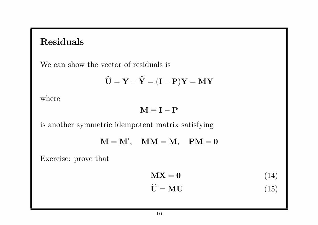
Residuals

We can show the vector of residuals is

U = Y− Y = (I−P)Y = MY

where

M ≡ I−P

is another symmetric idempotent matrix satisfying

M = M′, MM = M, PM = 0

Exercise: prove that

MX = 0 (14)

U = MU (15)

16

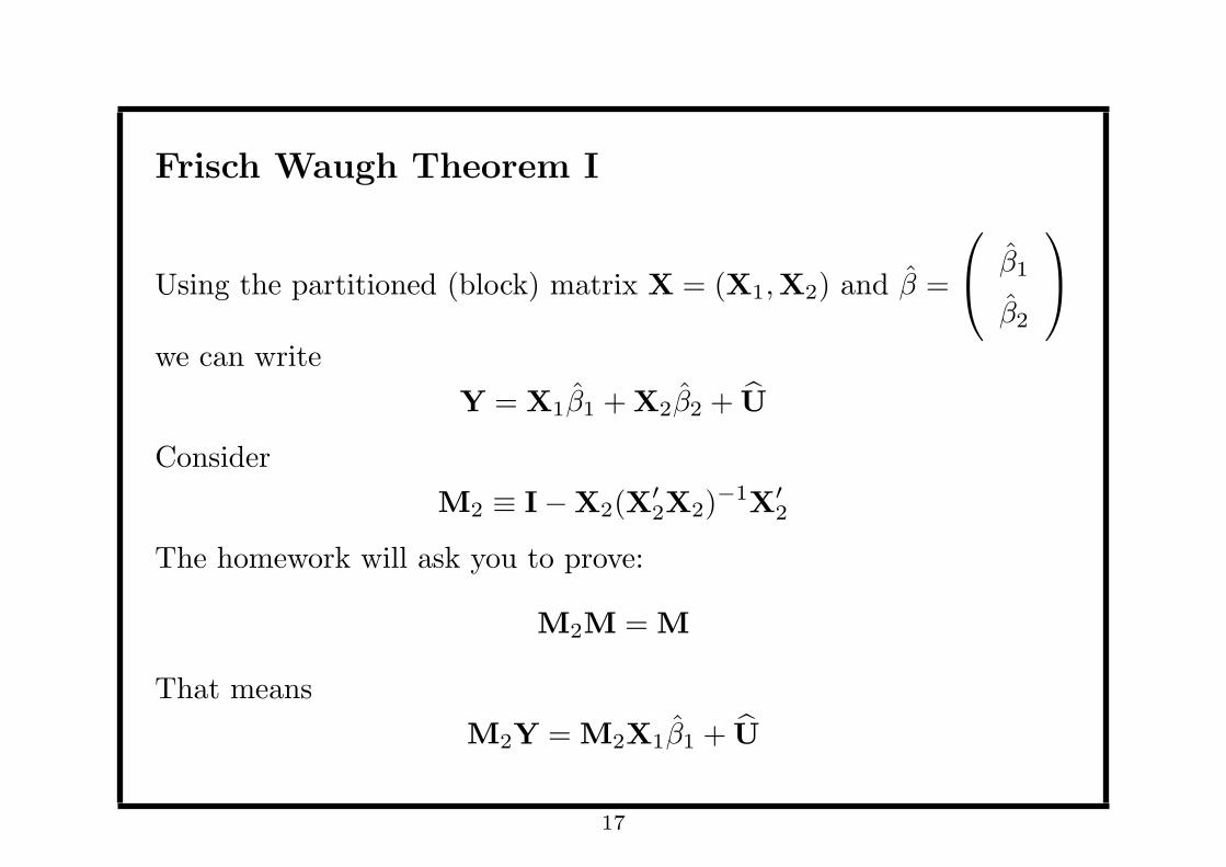
Frisch Waugh Theorem I

Using the partitioned (block) matrix X = (X1,X2) and β =

β1

β2

we can write

Y = X1β1 +X2β2 + U

Consider

M2 ≡ I−X2(X′2X2)

−1X′2

The homework will ask you to prove:

M2M = M

That means

M2Y = M2X1β1 + U

17

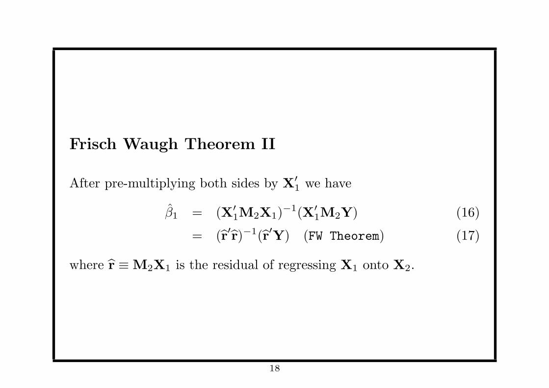
Frisch Waugh Theorem II

After pre-multiplying both sides by X′1 we have

β1 = (X′1M2X1)

−1(X′1M2Y) (16)

= (r′r)−1(r′Y) (FW Theorem) (17)

where r ≡ M2X1 is the residual of regressing X1 onto X2.

18

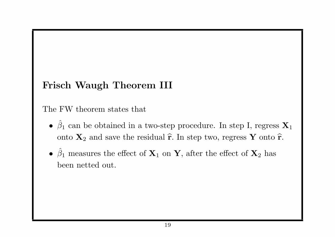
Frisch Waugh Theorem III

The FW theorem states that

• β1 can be obtained in a two-step procedure. In step I, regress X1

onto X2 and save the residual r. In step two, regress Y onto r.

• β1 measures the effect of X1 on Y, after the effect of X2 has

been netted out.

19

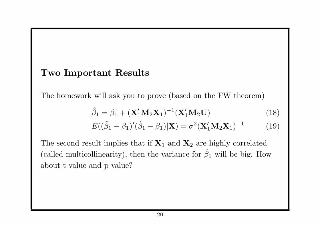
Two Important Results

The homework will ask you to prove (based on the FW theorem)

β1 = β1 + (X′1M2X1)

−1(X′1M2U) (18)

E((β1 − β1)′(β1 − β1)|X) = σ2(X′

1M2X1)−1 (19)

The second result implies that if X1 and X2 are highly correlated

(called multicollinearity), then the variance for β1 will be big. How

about t value and p value?

20

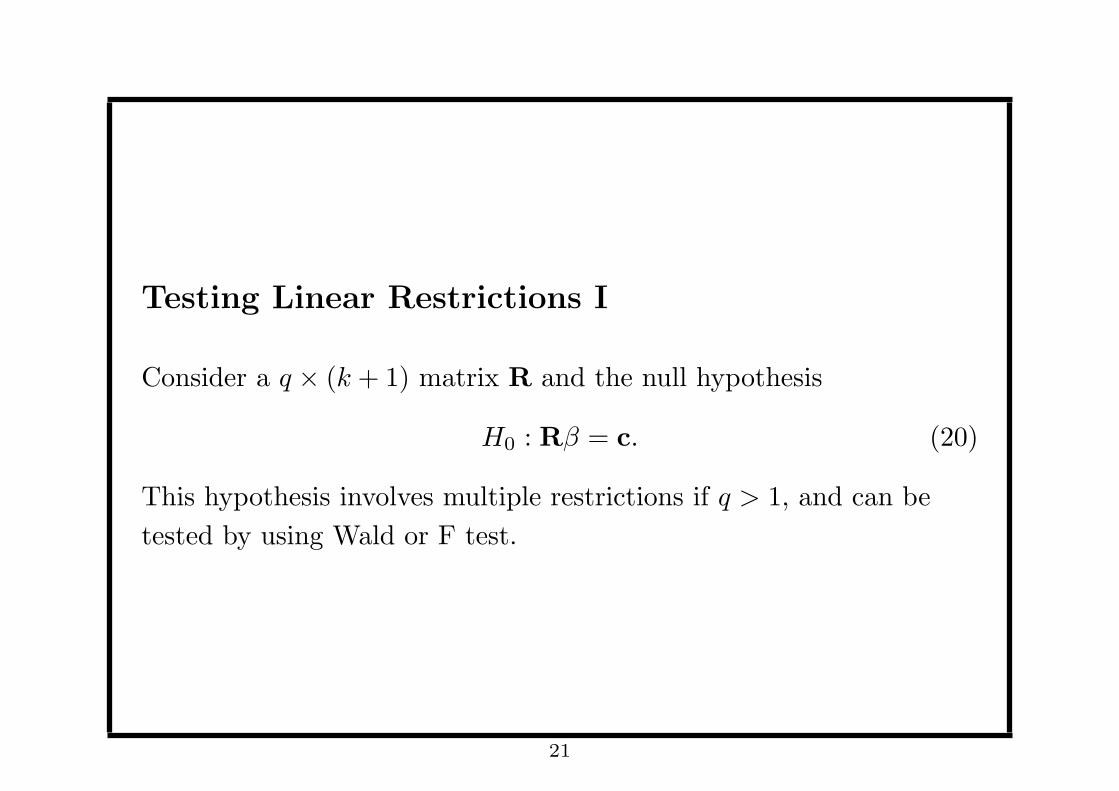
Testing Linear Restrictions I

Consider a q × (k + 1) matrix R and the null hypothesis

H0 : Rβ = c. (20)

This hypothesis involves multiple restrictions if q > 1, and can be

tested by using Wald or F test.

21

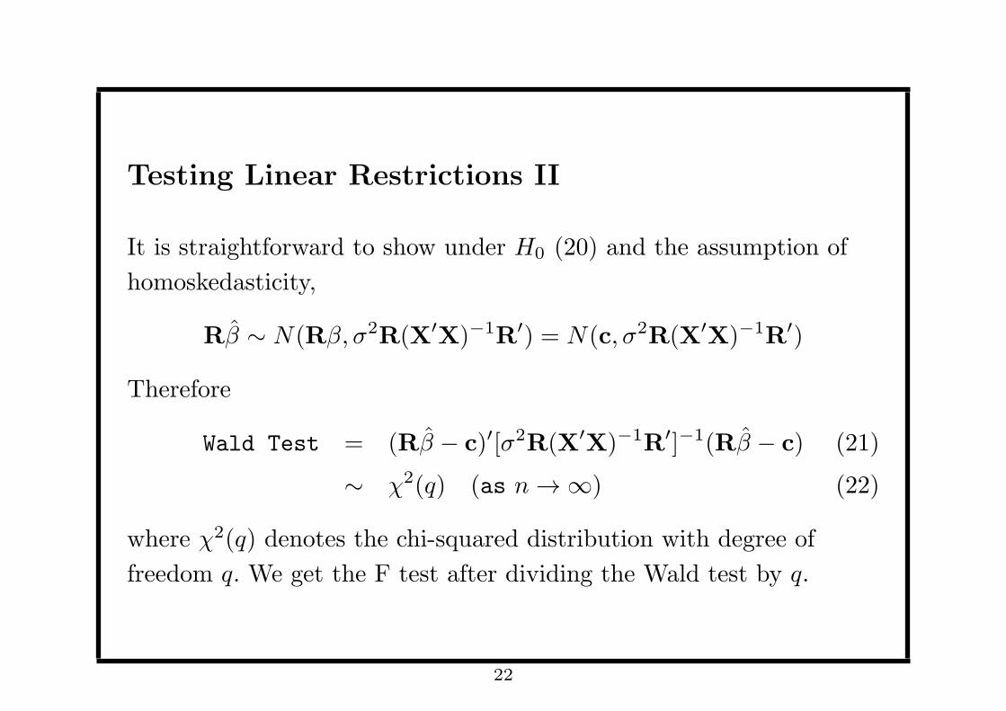
Testing Linear Restrictions II

It is straightforward to show under H0 (20) and the assumption of

homoskedasticity,

Rβ ∼ N(Rβ, σ2R(X′X)−1R′) = N(c, σ2R(X′X)−1R′)

Therefore

Wald Test = (Rβ − c)′[σ2R(X′X)−1R′]−1(Rβ − c) (21)

∼ χ2(q) (as n → ∞) (22)

where χ2(q) denotes the chi-squared distribution with degree of

freedom q. We get the F test after dividing the Wald test by q.

22

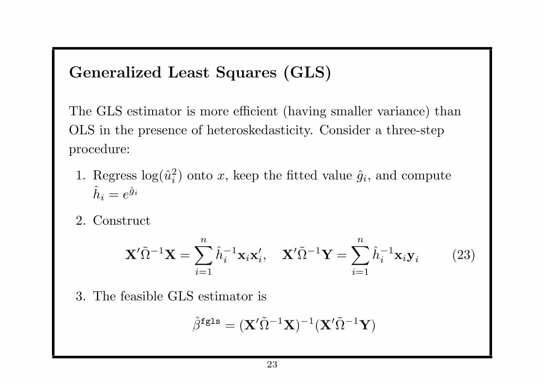
Generalized Least Squares (GLS)

The GLS estimator is more efficient (having smaller variance) than

OLS in the presence of heteroskedasticity. Consider a three-step

procedure:

1. Regress log(u2i ) onto x, keep the fitted value gi, and compute

hi = egi

2. Construct

X′Ω−1X =n∑

i=1

h−1i xix

′i, X′Ω−1Y =

n∑i=1

h−1i xiyi (23)

3. The feasible GLS estimator is

βfgls = (X′Ω−1X)−1(X′Ω−1Y)

23

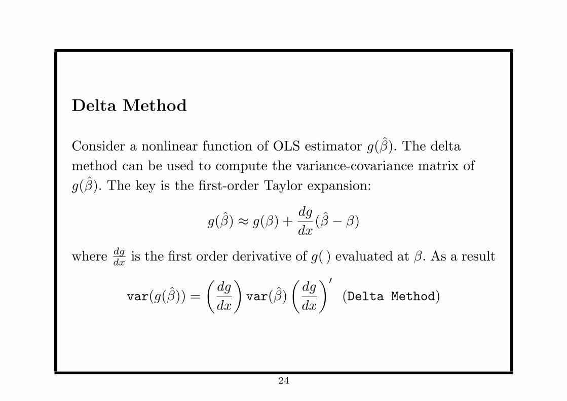
Delta Method

Consider a nonlinear function of OLS estimator g(β). The delta

method can be used to compute the variance-covariance matrix of

g(β). The key is the first-order Taylor expansion:

g(β) ≈ g(β) +dg

dx(β − β)

where dgdx is the first order derivative of g( ) evaluated at β. As a result

var(g(β)) =

(dg

dx

)var(β)

(dg

dx

)′

(Delta Method)

24