Embed Size (px)
Citation preview

UDC 621CODEN: MINSC5
In print: ISSN 1857 – 5293 On line: ISSN 1857 – 9191
MECHANICAL ENGINEERING
МАШИНСКО
ИНЖЕНЕРСТВО
SCIENTIFIC JOURNAL НАУЧНО СПИСАНИЕ
Volume 32 Number 1 Skopje, 2014

Mech. Eng. Sci. J. Vol. No. pp. Skopje 32 1 1–120 2014 Маш. инж. науч. спис. Год. Број стр. Скопје
MECHANICAL ENGINEERING – SCIENTIFIC JOURNAL МАШИНСКО ИНЖЕНЕРСТВО – НАУЧНО СПИСАНИЕ
Published by
Faculty of Mechanical Engineering, Ss. Cyril and Methodius University in Skopje, Republic of Macedonia Издава
Машински факултет, Универзитет „Св. Кирил и Методиј” во Скопје, Република Македонија
Published twice yearly – Излегува два пати годишно
INTERNATIONAL EDITORIAL BOARD – МЕЃУНАРОДЕН УРЕДУВАЧКИ ОДБОР Slave Armenski (Faculty of Mechanical Engineering, Ss. Cyril and Methodius University in Skopje, Skopje,
R. Macedonia), Aleksandar Gajić (Faculty of Mechanical Engineering, University of Belgrade, Belgrade, Serbia), Čedomir Duboka (Faculty of Mechanical Engineering, University of Belgrade, Belgrade, Serbia), Maslina Daruš
(Faculty of Science and Technology, University Kebangsaan Malaysia, Bangi, Malaysia), Robert Minovski (Faculty of Mechanical Engineering, Ss. Cyril and Methodius University in Skopje, Skopje, R. Macedonia), Wilfried Sihn (Institute
of Management Science, Vienna University of Technology, Vienna, Austria), Ivan Juraga (Faculty of Mechanical Engineering and Naval Architecture, University of Zagreb, Zagreb, Croatia), Janez Kramberger (Faculty
of Mechanical Enginneering, University of Maribor, Maribor, Slovenia), Karl Kuzman (Faculty of Mechanical Engineering, University of Ljubljana, Ljubljana, Slovenia), Clarisse Molad (University of Phoenix, Phoenix, Arizona, USA), Todor
Neshkov (Faculty of Mechanical Engineering, Technical University of Sofia, Sofia, Bulgaria), Zlatko Petreski (Faculty of Mechanical Engineering, Ss. Cyril and Methodius University in Skopje, Skopje, R.
Macedonia), Miroslav Plančak (Faculty of Technical Sciences, University of Novi Sad, Novi Sad, Serbia), Remon Pop-Iliev (Faculty of Engineering and Applied Science, University of Ontario Institute of Technology, Oshawa,
Ontario, Canada), Predrag Popovski (Faculty of Mechanical Engineering, Ss. Cyril and Methodius University in Skopje, Skopje, R. Macedonia), Dobre Runčev (Faculty of Mechanical Engineering, Ss. Cyril and Methodius University in Skopje, Skopje, R. Macedonia), Aleksandar Sedmak (Faculty of Mechanical Engineering, University of Belgrade,
Belgrade, Serbia), Ilija Ćosić (Faculty of Technical Sciences, University of Novi Sad, Novi Sad, Serbia), Rolf Steinhilper (Faculty of Engineering Science, University of Bayreuth, Bayreuth, Germany)
Editor in Chief Одговорен уредник Assoc. Prof. Igor Gjurkov, Ph.D Вон. проф. д-р. Игор Ѓурков
Co-editor in Chief Заменик одговорен уредник Assoc. Prof. Darko Danev, Ph.D Вон. проф. д-р. Дарко Данев
Ass. Prof. Dame Dimitrovski, Ph.D., secretary Доц. д-р Даме Димитровски, секретар
Technical editor managing Технички уредник Blagoja Bogatinoski Благоја Богатиноски
Lectors Лектура
Georgi Georgievski (Macedonian) Георги Георгиевски (македонски)
Proof-reader Коректор Alena Georgievska Алена Георгиевска
UDC: "St. Kliment Ohridski" Library – Skopje УДК: НУБ „Св.. Климент Охридски“ – Скопје
Copies: 300 Тираж: 300 Price: 520 denars Цена: 520 денари
Address Адреса
Faculty of Mechanical Engineering Машински факултет (Mechanical Engineering – Scientific Journal) (Машинско инженерство – научно списание)
Editor in Chief Одговорен уредник P.O.Box 464 пошт. фах 464
MK-1001 Skopje, Republic of Macedonia МК-1001 Скопје, Република Македонија Mech. Eng. Sci. J. is indexed/abstracted in INIS (International Nuclear Information System)
www.mf.ukim.edu.mk

MECHANICAL ENGINEERING – SCIENTIFIC JOURNAL FACULTY OF MECHANICAL ENGINEERING, SKOPJE, REPUBLIC OF MACEDONIA
МАШИНСКО ИНЖЕНЕРСТВО – НАУЧНО СПИСАНИЕ
МАШИНСКИ ФАКУЛТЕТ, СКОПЈЕ, РЕПУБЛИКА МАКЕДОНИЈА
Mech. Eng. Sci. J. Vol. No. pp. Skopje 32 1 1–120 2014 Маш. инж. науч. спис. Год. Број стр. Скопје
TABLE OF CONTENTS (С О Д Р Ж И Н А)
447 – Goce Tasevski, Zlatko Petreski, Dejan Šiškovski Simulation of an actuator & drive of a wire drawing machine’s mechatronic system using Matlab/Simulink (Симулација на актуатор од мехатронички систем на машина за извлекување на жица со употреба на Matlab/Simulink) ..........................................................................1–7
448 – Mite Tomov, Piotr Cichosz, Mikolaj Kuzinovski Comparison of contact skidded and skidless techniques which are used for surface roughness characterization (Споредба на контактните техники со лизгач и без лизгач кои се користат за карактеризација на рапавоста на површините)..............................................................9–15
449 – Mohammad Amin Rashidifar, Ali Amin Rashidifar Non-collocated fuzzy logic and input shaping control strategy for elastic joint manipulator: vibration suppression and time response analysis (Фазилогичен управувачки алгоритам со оформување на влезот за манипулатор со еластична врска: придушување на вибрации и анализа на временски одзив).....17–24
450 – Ali Belhocine, Abd Rahim Abu Bakar, Mostefa Bouchetara Structural and contact analysis of disc brake assembly during single stop braking event (Структурна и контактна анализа на склоп на кочници со дискови за време на единично сoпирање) ..................................................................................................25–33
451 – Dame Dimitrovski, Goran Dimeski Use of natural gas as a contribution to reducing emissions (Употреба на природен гас како придонес за намалување на емисиите)..................35–44
452 – Aleksandar Petrovski, Atanas Kočov, Valentina Žileska Pančovska Sustainable improvement of the energy efficiency of an existing building (Одржливо подобрување на енергетската ефикасност на постоен објект) ...............45–49
453 – Kristina Jakimovska, Igor Gjurkov Development of life cycle costing framework for user's costs in motor vehicles (Развој на структура на трошоци на животен циклус во поглед на трошоците на корисниците на моторните возила) ..........................................................................51–56

454 – Filip Popovski, Igor Nedelkovski Comparation of several models for interaction in virtual reality (Споредба на неколку модели за интеракција во виртуелна реалност) ....................57–63
455 – Darko Babunski, Atanasko Tuneski, Emil Zaev Comparison of simulated and measured response of load rejection on a hydro power plant model with mixed mode nonlinear controller (Споредба на симулиран и измерен одзив при одбивање на оптоварување на модел на хидроелектрична постројка со комбиниран нелинеарен управувач) .........65–69
456 – Goran Stanković, Stojan Petelin, Marko Perkovič, Peter Vidmar Advanced evacuation model managed through fuzzy logic during an accident in LNG terminal (Напреден евакуационен модел управуван преку fuzzy-логика при незгода во терминал за течен природен гас) .............................................................................71–79
457 – Goran Stanković, Stojan Petelin, Marko Perkovič, Peter Vidmar The influence of the technologically advanced evacuation models on the risk analyses during accidents in LNG terminal (Влијание на технолошки напредни евакуациони модели врз безбедносните анализи на незгоди во терминал за течен природен гас) ...........................................81–89
458 – Dame Dimitrovski, Elena Kitanovska, Mile Dimitrovski, Done Taševski Emission of carbon dioxide from diesel engines with emphasis on emissions in Republic of Macedonia (Загадување од дизел-мотори со внатрешно согорување со осврт на емисиите во Република Македонија) ......................................................................................... 91–98
459 – Bojan R. Jovanovski, Igor Nikoloski, Radmil Polenakovik, Trajče Velkovski, Emilija Nikoloska Training needs of women entrepreneurs in the Western Balkans, Turkey and Moldova (Потреба од обука на жените претприемачи во земјите од Западен Балкан, Турција и Молдавија).................................................................................................. 99–108
460 – Dejan Krstev, Radmil Polenakovik, Mirjana Golomeova Vehicle routing and scheduling – The traveling salesman problem (Рутирање и распоред на возило – проблем на трговски патник) ..........................109–117
Instructions for authors ......................................................................................................119–120

12:30:41 PM
Mechanical Engineering – Scientific Journal, Vol. 32, No. 1, pp. 1–7 (2014) CODEN: MINSC5 – 447 In print: ISSN 1857–5293 Received: September 24, 2013 On line: ISSN 1857–9191 Accepted: Feбruary 20, 2014 UDC: 004.942:621.778.1.06–523.8
Original scientific paper
SIMULATION OF AN ACTUATOR & DRIVE OF A WIRE DRAWING MACHINE’S MECHATRONIC SYSTEM USING MATLAB/SIMULINK
Goce Tasevski, Zlatko Petreski, Dejan Šiškovski
Institute for Mechanics, Faculty of Mechanical Engineering, "Ss. Cyril and Methodius" University in Skopje, P.O. box 464, 1000 Skopje, Republic of Macedonia
A b s t r a c t: Simulation of a mechatronic system actuator, implemented in a wire drawing machine, devel-oped in Matlab/Simulink environment is presented in this paper. AC induction motor with vector control drive is cho-sen as an actuator. Mathematical model of the actuator is expressed in d-q reference frame rotating at synchronous speed. Diagrams for calculation of the important parameters for the simulation of the actuator were constructed. Simulation results from the model behaviour were discussed in comparison with the specified parameters by the manufacturer of the existing actuator integrated in such mechatronic system.
Key words: actuator; induction motor; simulation; Matlab/Simulink; mechatronic system
СИМУЛАЦИЈА НА АКТУАТОР ОД МЕХАТРОНИЧКИ СИСТЕМ НА МАШИНА ЗА ИЗВЛЕКУВАЊЕ НА ЖИЦА СО УПОТРЕБА НА MATLAB/SIMULINK
А п с т р а к т: Направена е симулација и анализа на динамичкото однесување на еден актуатор од мехатроничкиот систем на машина за извлекување на жица со употреба на Matlab/Simulink. Како актуатор е избран AC индукционен мотор со векторско управување. Математичкиот модел на актуаторот е претставен во референтен систем d-q кој ротира со синхрона брзина. Направени се дијаграми за пресметка на важните параметри за симулација на актуаторот. На крајот се дискутирани резултатите од симулацијата во споредба со дадените параметри од производителот за постојниот актуатор вграден во таков мехатронички систем.
Клучни зборови: актуатор; индуктивен мотор; симулација; Matlab/Simulink; мехатронички систем
1. INTRODUCTION
Improving performance of wire drawing ma-chines, in terms of high drawing speed, has been usually achieved by the advances in the area of the die materials [1]. With the development of the mechatronic systems and functionalities nowadays, wire drawing machines could also increase the per-formances by introducing modern sensors and con-trol units in the system itself. With better monitor-ing of the motor parameters new advanced control algorithms could be developed in order to better control the system behaviour and increase drawing speeds.
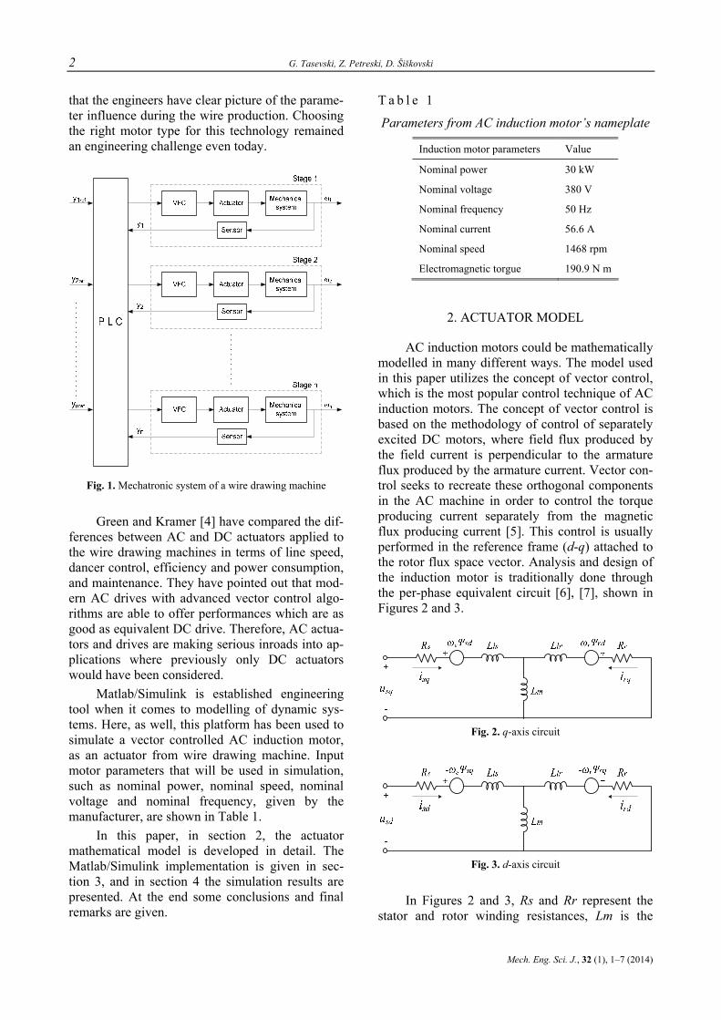
Mechatronic system of a modern wire draw-ing machine is presented in Figs.1 and 2. Dancer
arms or tuner rolls are used as sensors to indicate the current tension in the wire. These signals val-ues are compared with reference position values pre-set in the PLC controller. If any error occurs, PID controller together with variable frequency controllers gives command signals to the actuators, which are responsible for transforming the output of the control system into a controlling action on the mechanical system [2], [3], in order to maintain the wire tension.
One of the most important parts in the wire drawing machines are the motors that drive the blocks with different speeds to reduce the wire di-ameter. To increase performance of the machine, it is extremely important to develop a model of the entire system including the motors themselves, so
2 G. Tasevski, Z. Petreski, D. Šiškovski
Mech. Eng. Sci. J., 32 (1), 1–7 (2014)
that the engineers have clear picture of the parame-ter influence during the wire production. Choosing the right motor type for this technology remained an engineering challenge even today.
Fig. 1. Mechatronic system of a wire drawing machine
Green and Kramer [4] have compared the dif-ferences between AC and DC actuators applied to the wire drawing machines in terms of line speed, dancer control, efficiency and power consumption, and maintenance. They have pointed out that mod-ern AC drives with advanced vector control algo-rithms are able to offer performances which are as good as equivalent DC drive. Therefore, AC actua-tors and drives are making serious inroads into ap-plications where previously only DC actuators would have been considered.
Matlab/Simulink is established engineering tool when it comes to modelling of dynamic sys-tems. Here, as well, this platform has been used to simulate a vector controlled AC induction motor, as an actuator from wire drawing machine. Input motor parameters that will be used in simulation, such as nominal power, nominal speed, nominal voltage and nominal frequency, given by the manufacturer, are shown in Table 1.
In this paper, in section 2, the actuator mathematical model is developed in detail. The Matlab/Simulink implementation is given in sec-tion 3, and in section 4 the simulation results are presented. At the end some conclusions and final remarks are given.
T a b l e 1
Parameters from AC induction motor’s nameplate
Induction motor parameters Value
Nominal power 30 kW
Nominal voltage 380 V
Nominal frequency 50 Hz
Nominal current 56.6 A
Nominal speed 1468 rpm
Electromagnetic torgue 190.9 N m
2. ACTUATOR MODEL
AC induction motors could be mathematically modelled in many different ways. The model used in this paper utilizes the concept of vector control, which is the most popular control technique of AC induction motors. The concept of vector control is based on the methodology of control of separately excited DC motors, where field flux produced by the field current is perpendicular to the armature flux produced by the armature current. Vector con-trol seeks to recreate these orthogonal components in the AC machine in order to control the torque producing current separately from the magnetic flux producing current [5]. This control is usually performed in the reference frame (d-q) attached to the rotor flux space vector. Analysis and design of the induction motor is traditionally done through the per-phase equivalent circuit [6], [7], shown in Figures 2 and 3.
Fig. 2. q-axis circuit
Fig. 3. d-axis circuit
In Figures 2 and 3, Rs and Rr represent the stator and rotor winding resistances, Lm is the
Simulation of an actuator & drive of a wire drawing machine’s mechatronic system using Matlab/Simulink 3
Маш. инж. науч. спис., 32 (1), 1–7 (2014)
magnetizing inductance of the motor and Lls and Llr are the stator and rotor leakage inductances.
Considering the direct and quadrature axis (d-q) reference frame rotating at synchronous speed ωe, the model of the induction machine, as stated in [8] and [9], is given by the following equations:
Stator voltage equations:
sd s sd sd e sq
sq s sq sq e sd
du R idtdu R idt
ω
ω
= + Ψ − Ψ
= + Ψ + Ψ (1)
Rotor voltage equations:
( )
( )
0
0
rd r rd rd e r rq
rq r rq rq e r rd
du R idtdu R idt
ω ω
ω ω
= = + Ψ − − Ψ
= = + Ψ + − Ψ (2)
Stator and rotor flux linkage equations:
sqmrqrrq
sdmrdrrd
rqmsqssq
rdmsdssd
iLiLiLiL
iLiLiLiL
+=Ψ+=Ψ
+=Ψ+=Ψ
(3)
Electromagnetic torque:
( )sdrqsqrdr
me ii
LL
pT Ψ−Ψ= 5.1 (4)
3. MATLAB/SIMULINK IMPLEMENTATION
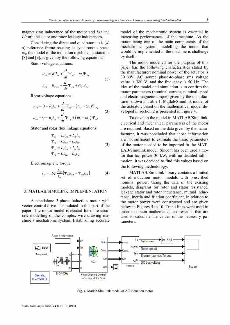
A standalone 3-phase induction motor with vector control drive is simulated in this part of the paper. The motor model is needed for more accu-rate modelling of the complex wire drawing ma-chine’s mechatronic system. Establishing accurate
model of the mechatronic system is essential in increasing performances of the machine. As the motor being one of the main components of the mechatronic system, modelling the motor that would be implemented in the machine is challenge by itself.
The motor modelled for the purpose of this paper has the following characteristics stated by the manufacturer: nominal power of the actuator is 30 kW, AC source phase-to-phase rms voltage value is 380 V, and the frequency is 50 Hz. The idea of the model and simulation is to confirm the motor parameters (nominal current, nominal speed and electromagnetic torque) given by the manufac-turer, shown in Table 1. Matlab/Simulink model of the actuator, based on the mathematical model de-veloped in section 2 is presented in Figure 4.
To develop the model in MATLAB/Simulink, electrical and mechanical parameters of the motor are required. Based on the data given by the manu-facturer, it was concluded that those information are not sufficient to estimate the basic parameters of the motor needed to be imported in the MAT-LAB/Simulink model. Since it has been used a mo-tor that has power 30 kW, with no detailed infor-mation, it was decided to find this values based on the following methodology.
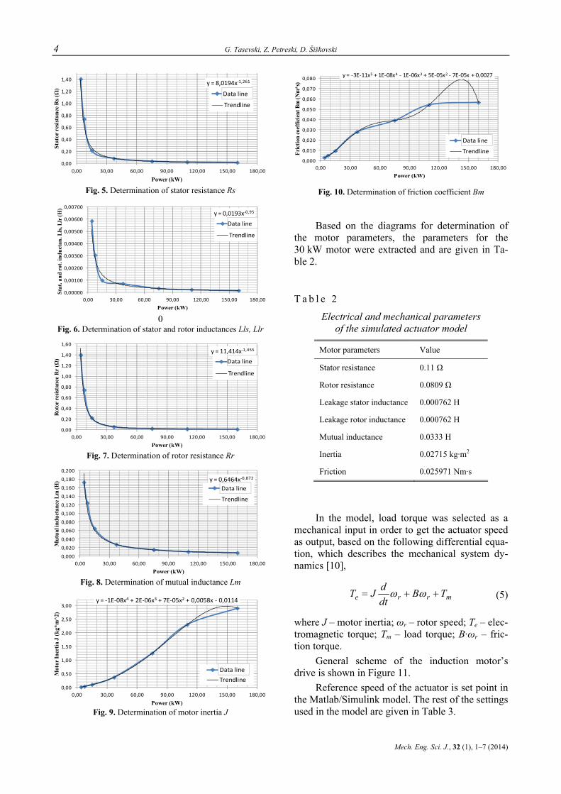
MATLAB/Simulink library contains a limited set of induction motor models with prescribed nominal power. Using the data of the existing models, diagrams for rotor and stator resistance, leakage stator and rotor inductance, mutual induc-tance, inertia and friction coefficient, in relation to the motor power were constructed and are given below in Figures 5 to 10. Trend lines were used in order to obtain mathematical expressions that are used to calculate the values of the necessary pa-rameters.
Fig. 4. Matlab/Simulink model of AC induction motor
4 G. Tasevski, Z. Petreski, D. Šiškovski
Mech. Eng. Sci. J., 32 (1), 1–7 (2014)
y = 8,0194x‐1,261
0,00
0,20
0,40
0,60
0,80
1,00
1,20
1,40
0,00 30,00 60,00 90,00 120,00 150,00 180,00
Stat
or re
sista
nce R
s (Ω
)
Power (kW)
Series1
Trendline
Data line
Fig. 5. Determination of stator resistance Rs
y = 0,0193x‐0,95
0,00000
0,00100
0,00200
0,00300
0,00400
0,00500
0,00600
0,00700
0,00 30,00 60,00 90,00 120,00 150,00 180,00
Stat
. and
rot.
indu
ctan
. Lls,
Llr
(H)
Power (kW)
Series1
Trendline
Data line
0 Fig. 6. Determination of stator and rotor inductances Lls, Llr
y = 11,414x‐1,455
0,00
0,20
0,40
0,60
0,80
1,00
1,20
1,40
1,60
0,00 30,00 60,00 90,00 120,00 150,00 180,00
Rot
or re
sista
nce
Rr
(Ω)
Power (kW)
Series1
Trendline
Data line
Fig. 7. Determination of rotor resistance Rr
y = 0,6464x‐0,872
0,000
0,020
0,040
0,060
0,080
0,100
0,120
0,140
0,160
0,180
0,200
0,00 30,00 60,00 90,00 120,00 150,00 180,00
Mut
ual i
nduc
tanc
e Lm
(H)
Power (kW)
Series1
Trendline
Data line
Fig. 8. Determination of mutual inductance Lm
y = ‐1E‐08x4 + 2E‐06x3 + 7E‐05x2 + 0,0058x ‐ 0,0114
0,00
0,50
1,00
1,50
2,00
2,50
3,00
0,00 30,00 60,00 90,00 120,00 150,00 180,00
Mot
or In
ertia
J (k
g*m
^2)
Power (kW)
Series1
Trendline
Data line
Fig. 9. Determination of motor inertia J
y = ‐3E‐11x5 + 1E‐08x4 ‐ 1E‐06x3 + 5E‐05x2 ‐ 7E‐05x + 0,0027
0,000
0,010
0,020
0,030
0,040
0,050
0,060
0,070
0,080
0,00 30,00 60,00 90,00 120,00 150,00 180,00
Fric
tion
coef
ficie
nt B
m (N
m*s
)
Power (kW)
Series1
Trendline
Data line
Fig. 10. Determination of friction coefficient Bm
Based on the diagrams for determination of the motor parameters, the parameters for the 30 kW motor were extracted and are given in Ta-ble 2.
T a b l e 2
Electrical and mechanical parameters of the simulated actuator model
Motor parameters Value
Stator resistance 0.11 Ω
Rotor resistance 0.0809 Ω
Leakage stator inductance 0.000762 H
Leakage rotor inductance 0.000762 H
Mutual inductance 0.0333 H
Inertia 0.02715 kg·m2
Friction 0.025971 Nm·s
In the model, load torque was selected as a
mechanical input in order to get the actuator speed as output, based on the following differential equa-tion, which describes the mechanical system dy-namics [10],
mrre TBdtdJT ++= ωω (5)
where J – motor inertia; ωr – rotor speed; Te – elec-tromagnetic torque; Tm – load torque; B·ωr – fric-tion torque.
General scheme of the induction motor’s drive is shown in Figure 11.
Reference speed of the actuator is set point in the Matlab/Simulink model. The rest of the settings used in the model are given in Table 3.

Simulation of an actuator & drive of a wire drawing machine’s mechatronic system using Matlab/Simulink 5
Маш. инж. науч. спис., 32 (1), 1–7 (2014)
Fig. 11. Scheme of induction motor’s drive
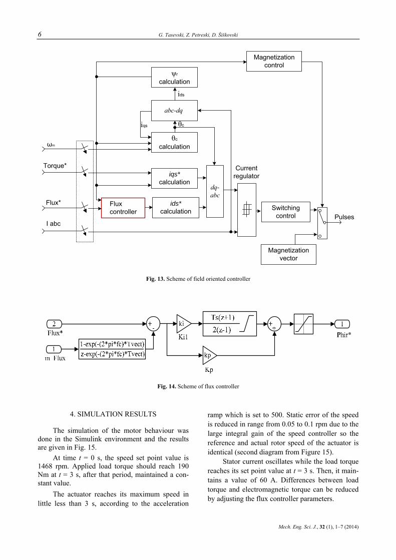
The dynamic response of the rotor speed and electromagnetic torque can be adjusted by the pro-portional and integral gains from the PI controllers in the speed and flux controllers. Speed controller and field oriented controller schemes are shown in Fig. 12 and Fig. 13, while Fig. 14 shows flux con-troller scheme. Tuning the parameters from speed and flux PI controllers is done by using trial and error method, and best fit parameters are inserted in Table 3, as well.
T a b l e 3
Parameters for speed and flux controller
Speed controller parameters Value
Acceleration ramp 500 rpm/s Deceleration ramp 500 rpm/s Proportional gain 10 Integral gain 2000
Flux controller prameters Value
Proportional gain 50 Integral gain 200
Fig. 12. Scheme of speed controller
6 G. Tasevski, Z. Petreski, D. Šiškovski
Mech. Eng. Sci. J., 32 (1), 1–7 (2014)
ψr
calculation
θc
calculation
iqs*calculation
Switching control
abc-dq
dq-abc
Fluxcontroller
Magnetization control
Current regulator
Magnetization vector
Torque*
Flux*
ωm
I abc
ids*calculation
Pulses
θciqs
ids
Fig. 13. Scheme of field oriented controller
Fig. 14. Scheme of flux controller
4. SIMULATION RESULTS
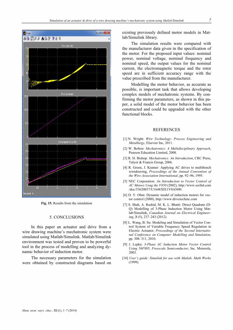
The simulation of the motor behaviour was done in the Simulink environment and the results are given in Fig. 15.
At time t = 0 s, the speed set point value is 1468 rpm. Applied load torque should reach 190 Nm at t = 3 s, after that period, maintained a con-stant value.
The actuator reaches its maximum speed in little less than 3 s, according to the acceleration
ramp which is set to 500. Static error of the speed is reduced in range from 0.05 to 0.1 rpm due to the large integral gain of the speed controller so the reference and actual rotor speed of the actuator is identical (second diagram from Figure 15).
Stator current oscillates while the load torque reaches its set point value at t = 3 s. Then, it main-tains a value of 60 A. Differences between load torque and electromagnetic torque can be reduced by adjusting the flux controller parameters.
Simulation of an actuator & drive of a wire drawing machine’s mechatronic system using Matlab/Simulink 7
Маш. инж. науч. спис., 32 (1), 1–7 (2014)
Fig. 15. Results from the simulation
5. CONCLUSIONS
In this paper an actuator and drive from a wire drawing machine’s mechatronic system were simulated using Matlab/Simulink. Matlab/Simulink environment was tested and proven to be powerful tool in the process of modelling and analyzing dy-namic behavior of induction motor.
The necessary parameters for the simulation were obtained by constructed diagrams based on
existing previously defined motor models in Mat-lab/Simulink library.
The simulation results were compared with the manufacturer data given in the specification of the motor. For the proposed input values: nominal power, nominal voltage, nominal frequency and nominal speed, the output values for the nominal current, the electromagnetic torque and the rotor speed are in sufficient accuracy range with the value prescribed from the manufacturer.
Modelling the motor behavior, as accurate as possible, is important task that allows developing complex models of mechatronic systems. By con-firming the motor parameters, as shown in this pa-per, a solid model of the motor behavior has been constructed and could be upgraded with the other functional blocks.
REFERENCES
[1] N. Wright: Wire Technology: Process Engineering and Metallurgy, Elsevier Inc, 2011.
[2] W. Bolton: Mechatronics: A Multidisciplinary Approach, Pearson Education Limited, 2008.
[3] R. H. Bishop: Mechatronics: An Introduction, CRC Press, Talyor & Francis Group, 2006.
[4] R. Green, J. Kramer: Applying AC drives to multibench wiredrawing, Proceedings of the Annual Convention of the Wire Association International, pp. 92–96, 1995.
[5] NEC Corporation: An Introduction to Vector Control of AC Motors Usng the V850 (2002), http://www.scribd.com /doc/53620037/U16483EE1V0AN00.
[6] D. Y. Ohm: Dynamic model of induction motors for vec-tor control (2000), http://www.drivetechinc.com
[7] S. Shah, A. Rashid, M. K. L. Bhatti: Direct Quadrate (D-Q) Modelling of 3-Phase Induction Motor Using Mat-lab/Simulink, Canadian Journal on Electrical Engineer-ing, 3 (5), 237–243 (2012).
[8] L. Wang, B. Su: Modeling and Simulation of Vector Con-trol System of Variable Frequency Speed Regulation in Electric Actuator, Proceedings of the Second Internatio-nal Conference on Computer Modelling and Simulation, pp. 308–311, 2010.
[9] J. Lepka: 3-Phase AC Induction Motor Vector Control Using 56F805, Freescale Semiconductor, Inc. Motorola, 2003.
[10] User’s guide: Simulink for use with Matlab, Math Works (1999).

Mechanical Engineering – Scientific Journal, Vol. 32, No. 1, pp. 9–15 (2014) CODEN: MINSC5 – 448 In print: ISSN 1857–5293 Received: October 10, 2013 On line: ISSN 1857–9191 Accepted: February 20, 2014 UDC: 621.9:620-408.8]:006.86
Original scientific paper
COMPARISON OF CONTACT SKIDDED AND SKIDLESS TECHNIQUES WHICH ARE USED FOR SURFACE ROUGHNESS CHARACTERIZATION
Mite Tomov1, Piotr Cichosz2, Mikolaj Kuzinovski1 1"Ss. Cyril and Methodius" University in Skopje, Faculty of Mechanical Engineering,
Karpoš II bb, P.O. box 464, 1001 Skopje, Republic of Macedonia 2Institute of Production Engineering and Automation of the Wrocław University of Technology,
Str. Lukasiewicza 3/5, 50-371 Wrocław, Polska [email protected]
A b s t r a c t: In this study included several dilemmas arising from the recommendations in the inter-national standards referring to surface roughness measurement with using skidded and skidless measure-ment instruments. Also, this paper explained the role and the impact of the skid as mechanical reference in the construction of the surface roughness measuring instruments. In order to determine the impact from the different constructive performances of the measurement instruments on the surface roughness value, are measured more periodic and non-periodic etalon surfaces representative of various machining process (turning, milling, grinding and lapping). Comparative analysis of the values and differences for the roughness parameters and primary profile parameters are displayed.
Key words: primary profile parameters; roughness parameters; skidded instruments; skidless instruments; periodic and non-periodic etalon surfaces
СПОРЕДБА НА КОНТАКТНИТЕ ТЕХНИКИ СО ЛИЗГАЧ И БЕЗ ЛИЗГАЧ КОИ СЕ КОРИСТАТ ЗА КАРАКТЕРИЗАЦИЈА НА РАПАВОСТА НА ПОВРШИНИТЕ
А п с т р а к т: Со оваа истражување се опфатени неколку дилеми кои произлегуваат од препораките во интернационалните стандарди, а кои се однесуваат на мерењето на рапавоста на површините со користење на мерни инструменти со лизгач и без лизгач. Во овој труд исто така се објаснетаиулогата и влијанието на лизгачот како механичка референца во конструкцијата на инс-трументите за мерење на рапавоста на површините. Мерени се повеќе периодични и непериодични еталон-површини претставници на различни обработки (стружење, глодање, брусење и зглобува-ње), а со цел да се определи влијанието врз вредностите на параметрите на рапавоста кое произле-гува од различните конструктивни изведби на мерните инструменти. Прикажана е компаративна анализа на вредностите и нивните разлики за параметрите на рапавост и параметрите на примар-ниот профил.
Клучни зборови: параметри на примарен профил; параметри на рапавост; инструменти со лизгач; инструменти без лизгач; периодични и непериодични еталон-површини
1. INTRODUCTION
The procedure (procedures) for obtaining the roughness profile, and thereby the roughness pa-rameters, has evolved together with the increase of
the capacities of measuring devices. In order to provide the conditions for comparability of the measured values of the roughness parameters, the procedures and recommendations used to measure and obtain the roughness profile are usually in-
10 M. Tomov, P. Cichosz, M. Kuzinovski
Mech. Eng. Sci. J., 32 (1), 9–15 (2014)
cluded in national standards on local level, or in-ternational standards on global level, which are usually harmonized with one another. However, these procedures and recommendations to be ap-plicable for different types of measuring instru-ments, they are general. According to ASME B46.1-2009 [1] all instruments that measure sur-face texture can be grouped into six groups of in-struments (first: profiling contact skidless instru-ments, second: profiling non-contact instruments, third: scanned probe microscopy, fourth: profiling contact skidded instruments, fifth: skidded instru-ments parameters only, and sixth: area averaging instruments). Of all the mentioned groups of meas-uring instruments for application purposes are used mostly contact skidded or skidless measuring in-struments.
The main purpose of these researches is to de-termine whether there are any differences as well as the size of those differences between the values of the roughness parameter obtained using two contact different measuring instruments (skidded and skidless), when measuring periodic and non-periodic etalon surfaces in identical measuring conditions.
2. THE FUNDAMENTAL DIFFERENCES BETWEEN SKIDDED AND SKIDLESS
INSTRUMENTS
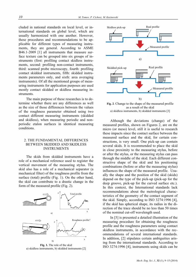
The skids from skidded instruments have a role of a mechanical reference used to register the vertical movement of the measuring stylus. The skid also has a role of a mechanical separator (a mechanical filter) of the roughness profile from the surface (total) profile (Fig. 1). On the other hand, the skid can contribute to a drastic change in the form of the measured profile (Fig. 2).
Roughness profile?
x
z
Total profile
x
z
a)
b) Fig. 1. The role of the skid
a) skidless instruments, b) skidded instruments [2]
Skidless pick-up Real profile
Measured profile
a)
Skidded pick-up Real profile
Measured profile
b)
Fig. 2. Change to the shape of the measured profile as a result of the skid
a) skidless instruments, b) skidded instruments [3]
Although the deviations (change) of the measured profiles, shown on Figures 2, are on the micro (or meso) level, still it is useful to research these impacts since the contact surface between the measured surface and the skid, for certain con-structions, is very small. One pick-up can contain several skids. It is recommended to place the skid in close proximity to the measuring stylus, before or after the stylus, or the measuring stylus can pass through the middle of the skid. Each different con-structive shape of the skid and his positioning combinations (before or after the measuring stylus) influences the shape of the measured profile. Usu-ally the shape and the position of the skid (skids) depend on the type of the pick-up (pick-up for the deep groove, pick-up for the curved surface etc.). In this context, the International standards lack recommendations about the metrological charac-teristics of the geometry of the contact segment of the skid. Simply, according to ISO 3274:1996 [4], if the skid has spherical shape, its radius in the di-rection of the trace should be no less than 50 times of the nominal cut-off wavelength used.
In [5] is presented a detailed illustration of the measuring procedure for obtaining the roughness profile and the roughness parameters using contact skidless instruments, in accordance with the rec-ommendations of several international standards. In addition, [2] stipulates certain ambiguities aris-ing from the international standards. According to ISO 3274:1996 [4], instruments using skids can be
Comparison of contact skidded and skidless techniques which are used for surface roughness characterization 11
Маш. инж. науч. спис., 32 (1), 9–15 (2014)
used for measuring roughness parameters only. On the other hand, the calculation of the values of the roughness parameters requires the determination of a mean reference line using a λc profile-filter, which means that the measured profile should un-dergo software filtration using a λc profile filter. How do we call the profile through which we draw the mean reference line using a λc profile filter? Is this the primary profile? Also, having in mind that it is not possible to isolate the noise from the signal during the measurement, again there is a need for software filtration using a λs profile filter. If we add the noise to the primary profile, do we get the total profile? Every measuring instrument has a λs profile-filter, and usually, in the case of portable instruments, this filter turns on automatically, without any activation by the metrologist. If, on top of this, we also add the software leveling of the measured profile (using the least squares method) which is the same as removing the nominal linear shape, then we get the total profile. Therefore, the question is: What kind of an initial profile is ob-tained when the using an instrument that uses a skid as a mechanical reference?
Precisely these remarks, directly related to the use of contact skidded and skidless instruments were the additional reason to implement this type of research.
3. EXPERIMENTAL INVESTIGATIONS
3.1. Measuring conditions
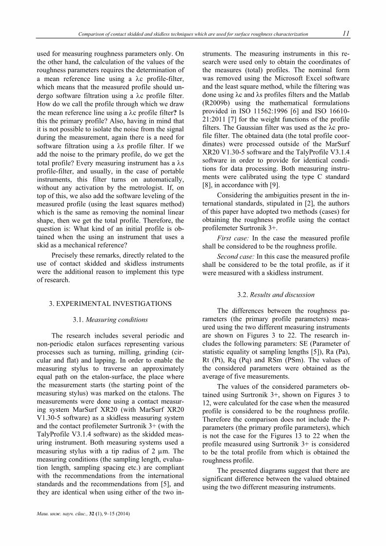
The research includes several periodic and non-periodic etalon surfaces representing various processes such as turning, milling, grinding (cir-cular and flat) and lapping. In order to enable the measuring stylus to traverse an approximately equal path on the etalon-surface, the place where the measurement starts (the starting point of the measuring stylus) was marked on the etalons. The measurements were done using a contact measur-ing system MarSurf XR20 (with MarSurf XR20 V1.30-5 software) as a skidless measuring system and the contact profilemeter Surtronik 3+ (with the TalyProfile V3.1.4 software) as the skidded meas-uring instrument. Both measuring systems used a measuring stylus with a tip radius of 2 µm. The measuring conditions (the sampling length, evalua-tion length, sampling spacing etc.) are compliant with the recommendations from the international standards and the recommendations from [5], and they are identical when using either of the two in-
struments. The measuring instruments in this re-search were used only to obtain the coordinates of the measures (total) profiles. The nominal form was removed using the Microsoft Excel software and the least square method, while the filtering was done using λc and λs profiles filters and the Matlab (R2009b) using the mathematical formulations provided in ISO 11562:1996 [6] and ISO 16610-21:2011 [7] for the weight functions of the profile filters. The Gaussian filter was used as the λc pro-file filter. The obtained data (the total profile coor-dinates) were processed outside of the MarSurf XR20 V1.30-5 software and the TalyProfile V3.1.4 software in order to provide for identical condi-tions for data processing. Both measuring instru-ments were calibrated using the type C standard [8], in accordance with [9].
Considering the ambiguities present in the in-ternational standards, stipulated in [2], the authors of this paper have adopted two methods (cases) for obtaining the roughness profile using the contact profilemeter Surtronik 3+.
First case: In the case the measured profile shall be considered to be the roughness profile.
Second case: In this case the measured profile shall be considered to be the total profile, as if it were measured with a skidless instrument.
3.2. Results and discussion
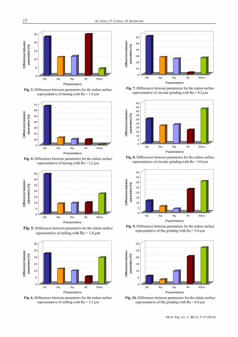
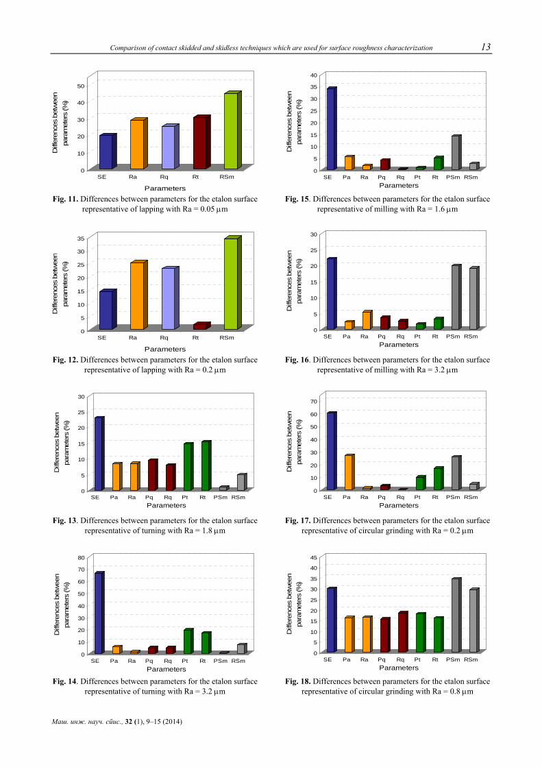
The differences between the roughness pa-rameters (the primary profile parameters) meas-ured using the two different measuring instruments are shown on Figures 3 to 22. The research in-cludes the following parameters: SE (Parameter of statistic equality ot sampling lengths [5]), Ra (Pa), Rt (Pt), Rq (Pq) and RSm (PSm). The values of the considered parameters were obtained as the average of five measurements.
The values of the considered parameters ob-tained using Surtronik 3+, shown on Figures 3 to 12, were calculated for the case when the measured profile is considered to be the roughness profile. Therefore the comparison does not include the P-parameters (the primary profile parameters), which is not the case for the Figures 13 to 22 when the profile measured using Surtronik 3+ is considered to be the total profile from which is obtained the roughness profile.
The presented diagrams suggest that there are significant difference between the valued obtained using the two different measuring instruments.
12 M. Tomov, P. Cichosz, M. Kuzinovski
Mech. Eng. Sci. J., 32 (1), 9–15 (2014)
0
5
10
15
20
25
Diff
eren
ces
betw
een
para
met
ers
(%)
SE Ra Rq Rt RSm
Parameters Fig. 3. Differences between parameters for the etalon surface
representative of turning with Ra = 1.8 µm
0
10
20
30
40
50
60
70
Diff
eren
ces
betw
een
para
met
ers
(%)
SE Ra Rq Rt RSm
Parameters Fig. 4. Differences between parameters for the etalon surface
representative of turning with Ra = 3.2 µm
0
5
10
15
20
25
30
35
Diff
eren
ces
betw
een
para
met
ers
(%)
SE Ra Rq Rt RSm
Parameters Fig. 5. Differences between parameters for the etalon surface
representative of milling with Ra = 1.6 µm
0
5
10
15
20
25
30
Diff
eren
ces
betw
een
para
met
ers
(%)
SE Ra Rq Rt RSm
Parameters Fig. 6. Differences between parameters for the etalon surface
representative of milling with Ra = 3.2 µm
0
10
20
30
40
50
60
Diff
eren
ces
betw
een
para
met
ers
(%)
SE Ra Rq Rt RSm
Parameters Fig. 7. Differences between parameters for the etalon surface
representative of circular grinding with Ra = 0.2 µm
0
5
10
15
20
25
30
35
40
45
50
Diff
eren
ces
betw
een
para
met
ers
(%)
SE Ra Rq Rt RSm
Parameters Fig. 8. Differences between parameters for the etalon surface
representative of circular grinding with Ra = 0.8 µm
0
5
10
15
20
25
30
35
40
Diff
eren
ces
betw
een
para
met
ers
(%)
SE Ra Rq Rt RSm
Parameters Fig. 9. Differences between parameters for the etalon surface
representative of flat grinding with Ra = 0.4 µm
0
5
10
15
20
25
30
Diff
eren
ces
betw
een
para
met
ers
(%)
SE Ra Rq Rt RSm
Parameters Fig. 10. Differences between parameters for the etalon surface
representative of flat grinding with Ra = 0.8 µm
Comparison of contact skidded and skidless techniques which are used for surface roughness characterization 13
Маш. инж. науч. спис., 32 (1), 9–15 (2014)
0
10
20
30
40
50
Diff
eren
ces
betw
een
para
met
ers
(%)
SE Ra Rq Rt RSm
Parameters Fig. 11. Differences between parameters for the etalon surface
representative of lapping with Ra = 0.05 µm
0
5
10
15
20
25
30
35
Diff
eren
ces
betw
een
para
met
ers
(%)
SE Ra Rq Rt RSm
Parameters Fig. 12. Differences between parameters for the etalon surface
representative of lapping with Ra = 0.2 µm
0
5
10
15
20
25
30
Diff
eren
ces
betw
een
para
met
ers
(%)
SE Pa Ra Pq Rq Pt Rt PSm RSm Parameters
Fig. 13. Differences between parameters for the etalon surface
representative of turning with Ra = 1.8 µm
0
10
20
30
40
50
60
70
80
Diff
eren
ces
betw
een
para
met
ers
(%)
SE Pa Ra Pq Rq Pt Rt PSm RSm Parameters
Fig. 14. Differences between parameters for the etalon surface representative of turning with Ra = 3.2 µm
0
5
10
15
20
25
30
35
40
Diff
eren
ces
betw
een
para
met
ers
(%)
SE Pa Ra Pq Rq Pt Rt PSm RSm Parameters
Fig. 15. Differences between parameters for the etalon surface representative of milling with Ra = 1.6 µm
0
5
10
15
20
25
30
Diff
eren
ces
betw
een
para
met
ers
(%)
SE Pa Ra Pq Rq Pt Rt PSm RSm Parameters
Fig. 16. Differences between parameters for the etalon surface
representative of milling with Ra = 3.2 µm
0
10
20
30
40
50
60
70
Diff
eren
ces
betw
een
para
met
ers
(%)
SE Pa Ra Pq Rq Pt Rt PSm RSm Parameters
Fig. 17. Differences between parameters for the etalon surface
representative of circular grinding with Ra = 0.2 µm
0
5
10
15
20
25
30
35
40
45
Diff
eren
ces
betw
een
para
met
ers
(%)
SE Pa Ra Pq Rq Pt Rt PSm RSm Parameters
Fig. 18. Differences between parameters for the etalon surface representative of circular grinding with Ra = 0.8 µm
14 M. Tomov, P. Cichosz, M. Kuzinovski
Mech. Eng. Sci. J., 32 (1), 9–15 (2014)
0
5
10
15
20
25
30
35
40
Diff
eren
ces
betw
een
para
met
ers
(%)
SE Pa Ra Pq Rq Pt Rt PSm RSm Parameters
Fig. 19. Differences between parameters for the etalon surface representative of flat grinding with Ra = 0.4 µm
0
5
10
15
20
25
30
Diff
eren
ces
betw
een
para
met
ers
(%)
SE Pa Ra Pq Rq Pt Rt PSm RSm Parameters
Fig. 20. Differences between parameters for the etalon surface representative of flat grinding with Ra = 0.8 µm
0
5
10
15
20
25
30
35
40
45
Diff
eren
ces
betw
een
para
met
ers
(%)
SE Pa Ra Pq Rq Pt Rt PSm RSm Parameters
Fig. 21. Differences between parameters for the etalon surface representative of lapping with Ra = 0.05 µm
0
2
4
6
8
10
12
14
16
18
20
Diff
eren
ces
betw
een
para
met
ers
(%)
SE Pa Ra Pq Rq Pt Rt PSm RSm Parameters
Fig. 22. Differences between parameters for the etalon surface representative of lapping with Ra = 0.2 µm
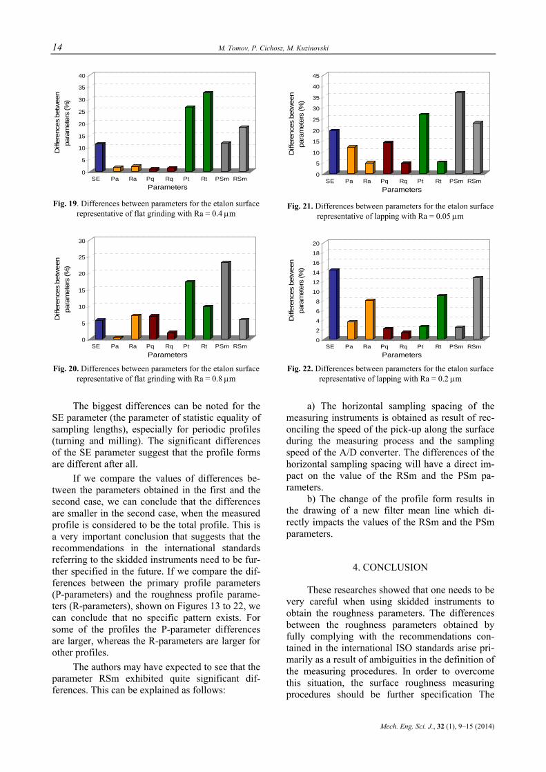
The biggest differences can be noted for the SE parameter (the parameter of statistic equality of sampling lengths), especially for periodic profiles (turning and milling). The significant differences of the SE parameter suggest that the profile forms are different after all.
If we compare the values of differences be-tween the parameters obtained in the first and the second case, we can conclude that the differences are smaller in the second case, when the measured profile is considered to be the total profile. This is a very important conclusion that suggests that the recommendations in the international standards referring to the skidded instruments need to be fur-ther specified in the future. If we compare the dif-ferences between the primary profile parameters (P-parameters) and the roughness profile parame-ters (R-parameters), shown on Figures 13 to 22, we can conclude that no specific pattern exists. For some of the profiles the P-parameter differences are larger, whereas the R-parameters are larger for other profiles.
The authors may have expected to see that the parameter RSm exhibited quite significant dif-ferences. This can be explained as follows:
a) The horizontal sampling spacing of the measuring instruments is obtained as result of rec-onciling the speed of the pick-up along the surface during the measuring process and the sampling speed of the A/D converter. The differences of the horizontal sampling spacing will have a direct im-pact on the value of the RSm and the PSm pa-rameters.
b) The change of the profile form results in the drawing of a new filter mean line which di-rectly impacts the values of the RSm and the PSm parameters.
4. CONCLUSION
These researches showed that one needs to be very careful when using skidded instruments to obtain the roughness parameters. The differences between the roughness parameters obtained by fully complying with the recommendations con-tained in the international ISO standards arise pri-marily as a result of ambiguities in the definition of the measuring procedures. In order to overcome this situation, the surface roughness measuring procedures should be further specification The

Comparison of contact skidded and skidless techniques which are used for surface roughness characterization 15
Маш. инж. науч. спис., 32 (1), 9–15 (2014)
large differences in the PSm (RSm) parameter lead us to the conclusion that maybe the calibration of the measuring instruments requires more than an overall calibration using one type of etalon, but rather calibration of the vertical readout of the in-strument should be separated from the horizontal. The values obtained for the differences between the considered parameters have shown no specific change patters.
REFERENCES
[1] ASME B46.1-2009. Surface texture (surface roughness, waviness, and lay). The American Society of Mechanical Engineers, New York, 2009.
[2] M. Kuzinovski, M. Tomov. Standardization – A mitigat-ing or a confusing circumstance in surface roughness measuring in the metal processing industry. International Journal of Industrial Engineering & Technology (IJIET). 3 (1), 37–42 (March 2013).
[3] M. Tomov. Contribution in development of the methods and measuring techniques for research of influential fac-
tors for identification of the surface topography. PhD dis-sertation, Skopje, 2013.
[4] ISO 3274:1996. Geometrical Product Specifications (GPS) – Surface texture: Profile method – Nominal char-acteristics of contact stylus instruments. International Or-ganization for Standardization, Geneva.
[5] Mite Tomov, Mikolaj Kuzinovski, Piotr Cichosz. A New Parameter of Statistic Equality of Sampling Lengths in Surface Roughness Measurement. Strojniški vestnik – Journal of Mechanical Engineering, 59 (5), 339–348 (2013).
[6] ISO 11562:1996. Geometrical Product Specifications (GPS) - Surface texture: Profile method – Metrological characteristics of phase correct filters. International Or-ganization for Standardization, Geneva.
[7] ISO 16610-21:2011. Geometrical Product Specifications (GPS) – Filtration: Linear profile filters: Gaussian fil-ters. International Organization for Standardization, Ge-neva.
[8] ISO 5436-1:2000; Geometrical Product Specifications (GPS) – Surface texture: Profile method; Measurement standards – Part 1: Material measures.
[9] ISO 12179:2000; Geometrical Product Specifications (GPS) – Surface texture: Profile method – Calibration of contact (stylus) instruments.

Mechanical Engineering – Scientific Journal, Vol. 32, No. 1, pp. 17–24 (2014) CODEN: MINSC5 – 449 In print: ISSN 1857–5293 Received: November 7, 2013 On line: ISSN 1857–9191 Accepted: February 20, 2014 UDC: 681.515.8:534.83]:621.8–27
Original scientific paper
NON-COLLOCATED FUZZY LOGIC AND INPUT SHAPING CONTROL STRATEGY FOR ELASTIC JOINT MANIPULATOR: VIBRATION SUPPRESSION
AND TIME RESPONSE ANALYSIS
Mohammad Amin Rashidifar1, Ali Amin Rashidifar2 1Faculty of Mechanical Engineering, Islamic Azad University, SHADEGAN Branch, SHADEGAN, Iran,
2Computer Science, Islamic Azad University, SHADEGAN Branch, SHADEGAN, Iran [email protected] // [email protected]
A b s t r a c t: Conventional model-based control strategies are very complex and difficult to synthesize due to high complexity of the dynamics of robots manipulator considering joint elasticity. This paper presents investigations into the development of hybrid control schemes for trajectory tracking and vibration control of a flexible joint ma-nipulator. To study the effectiveness of the controllers, initially a collocated proportional-derivative (PD)-type Fuzzy Logic Controller (FLC) is developed for tip angular position control of a flexible joint manipulator. This is then ex-tended to incorporate a non-collocated Fuzzy Logic Controller and input shaping scheme for vibration reduction of the flexible joint system. The positive zero-vibration-derivative-derivative (ZVDD) shaper is designed based on the properties of the system. Simulation results of the response of the flexible joint manipulator with the controllers are presented in time and frequency domains. The performances of the hybrid control schemes are examined in terms of input tracking capability, level of vibration reduction and time response specifications. Finally, a comparative as-sessment of the control techniques is presented and discussed.
Key words: elastic joint; vibration control; input shaping; fuzzy logic control
ФАЗИЛОГИЧЕН УПРАВУВАЧКИ АЛГОРИТАМ СО ОФОРМУВАЊЕ НА ВЛЕЗОТ ЗА МАНИПУЛАТОР СО ЕЛАСТИЧНА ВРСКА: ПРИДУШУВАЊЕ НА ВИБРАЦИИ
И АНАЛИЗА НА ВРЕМЕНСКИ ОДЗИВ
А п с т р а к т: Конвенционалните управувачки алгоритми базирани на модел се многу комплексни и тешки за креирање поради сложеноста на динамиката на манипулатори земајќи ја предвид еластичната врска. Овој труд презентира инстражувања од развој на хибридни управувачки алгоритми за следење на траекторија и контрола на вибрациите на манипулатор со еластична врска. За испитување на ефективноста на управува-чот, најпрво е развиен PD-тип на фази-управувач за управување со аголната позиција на манипулаторот со еластична врска. Потоа овој концепт е проширен со вклучување фази-управувач и управувач со оформување на влезот за намалување на вибрациите на системот. Управувачот со оформување на влезот е проектиран спо-ред карактеристиките на системот. Резултатите од симулацијата се презентирани во временски и фреквенцис-ки домен. Перформансите на хибридниот управувачки алгоритам се анализирани врз основа на способноста за следење, нивото на намалување на вибрациите и временскиот одзив. На крајот е презентирана и дискути-рана компаративна анализа на управувачките техники.
Клучни зборови: еластична врска, контрола на вибрации, управување со оформување на влез, управување со фази-логика
1. INTRODUCTION
Nowadays, elastic joint manipulators have re-ceived a thorough attention due to their light
weight, high manoeuvrability, flexibility, high power efficiency, and large number of applica-tions. However, controlling such systems still faces numerous challenges that need to be addressed.
18 M. Amin Rashidifar, A. Amin Rashidifar
Mech. Eng. Sci. J., 32 (1), 17–24 (2014)
The control issue of the flexible joint is to design the controller so that link of robot can track a pre-scribed trajectory precisely with minimum vibra-tion to the link. In order to achieve these objec-tives, various methods using different technique have been proposed. Yim [1], Oh and Lee [2] pro-posed adaptive output-feedback controller based on a backstepping design. This technique is pro-posed to deal with parametric uncertainty in flexi-ble joint. The relevant work also been done by Ghorbel et al. [3]. Lin and Yuan [4] and Spong et al. [5] introduced non linear control approach using namely feedback linearization technique and the integral manifold technique respectively. A robust control design was reported by Tomei [6] by using simple PD control and Yeon and Park [7] by ap-plying robust H∞ control. Among the proposed techniques, the conventional feedback control de-sign handled by pole placement method and LQR method also have been widely used due to its sim-plicity implementation. Particularly in LQR method, the values of Q and R matrices are pre-specified to determine optimal feedback control gain via Riccati equation [8].
On another aspect, an acceptable system per-formance with reduced vibration that accounts for system changes can be achieved by developing a hybrid control scheme that caters for rigid body motion and vibration of the system independently. This can be realized by utilizing control strategies consisting of either non-collocated with collocated feedback controllers or feed-forward with feedback controllers. In both cases, the former can be used for vibration suppression and the latter for input tracking of a flexible manipulator. A hybrid collo-cated and non-collocated controller has widely been proposed for control of a flexible structure [8, 9, 10]. The works have shown that the control structure gives a satisfactory system response with significant vibration reduction as compared to a response with a collocated controller. A feedback control with a feed-forward control to regulate the position of a flexible structure has previously been proposed [11, 12]. A control law partitioning scheme which uses end-point sensing device has also been reported [13]. The scheme uses end-point position signal in an outer loop controller to con-trol the flexible modes, whereas the inner loop controls the rigid body motion independent of the flexible dynamics of the manipulator.
This paper presents investigation into the de-velopment of control schemes for trajectory track-ing of tip angular position and vibration control of
flexible joint manipulator. Control strategies based on collocated PD-type FLC with non-collocated fuzzy and the combination of collocated PD-type FLC with input shaping are investigated. For non-collocated control, a deflection angle feedback through a fuzzy logic control configuration whereas input shaping is utilised as a feed-forward scheme for reducing a deflection effect. A simula-tion environment is developed within Simulink and Matlab for evaluation of performance of the con-trol schemes. The rest of the paper is structured as follows: Section 2 provides a brief description of the single-link flexible joint manipulator system considered in this study. Section 3 describes the modelling of the system derived using Euler-Lagrange formulation. The composite collocated PD-type FLC with fuzzy logic control and input shaping scheme are described in Section 4. Simula-tion results and comparative assessment are pre-sented in Section 5 and the paper is concluded in Section 6.
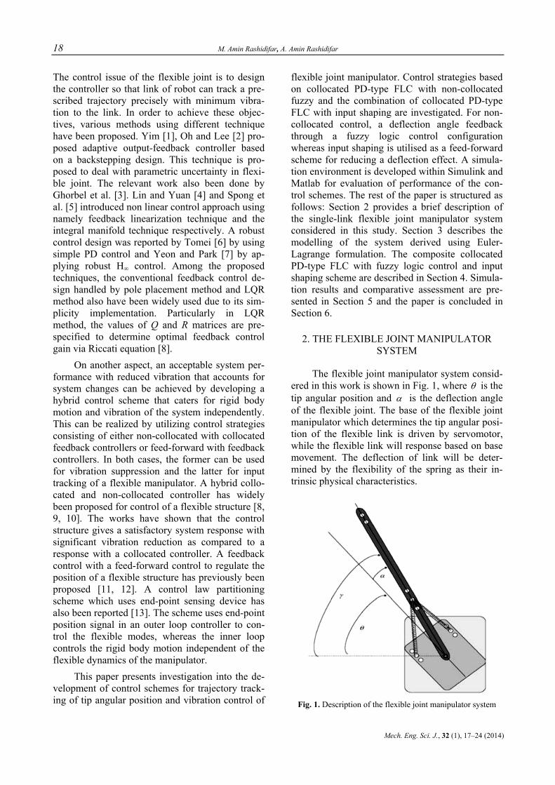
2. THE FLEXIBLE JOINT MANIPULATOR SYSTEM
The flexible joint manipulator system consid-ered in this work is shown in Fig. 1, where θ is the tip angular position and α is the deflection angle of the flexible joint. The base of the flexible joint manipulator which determines the tip angular posi-tion of the flexible link is driven by servomotor, while the flexible link will response based on base movement. The deflection of link will be deter-mined by the flexibility of the spring as their in-trinsic physical characteristics.
Fig. 1. Description of the flexible joint manipulator system
Non-collocated fuzzy logic and input shaping control strategy for elastic joint manipulator: vibration suppression and time response analysis 19
Маш. инж. науч. спис., 32 (1), 17–24 (2014)
3. MODELLING OF THE FLEXIBLE JOINT MANIPULATOR
This section provides a brief description on the modelling of the flexible joint manipulator sys-tem, as a basis of a simulation environment for de-velopment and assessment of the hybrid Fuzzy Logic control techniques. The Euler-Lagrange formulation is considered in characterizing the dy-namic behaviour of the system.
The linear model of the uncontrolled system can be represented in a state-space form [15] as shown in equation (1), that is
x Ax Buy Cx= +=
(1)
with the vector T
x θ α θ α⎡ ⎤= ⎣ ⎦ and the matri-
ces A, B and C are given by
[ ]
2
2
0 0 1 00 0 0 1
0 0
0 0
0 0 , 1 0 0 0
stiff m g t m g eq m
eq eq m
stiff eq arm m g t m g eq m
eq arm eq m
m g t g m g t g
eq m eq m
K η η K K K B RA J J R
K (J J ) η η K K K B RJ J J R
η η K K η η K KB C
J R J R
⎡ ⎤⎢ ⎥⎢ ⎥⎢ ⎥− +⎢ ⎥=⎢ ⎥⎢ ⎥
− + +⎢ ⎥⎢ ⎥⎣ ⎦
⎡ ⎤−= =⎢ ⎥⎢ ⎥⎣ ⎦
(2)
In equation (1), the input u is the input volt-age of the servomotor, mV , which determines the flexible joint manipulator base movement. In this study, the values of the parameters are defined in Table 1.
T a b l e 1 System parameters
Symbol QUANTITY Value
Rm Armature Resistance (Ohm) 2.6 Km Motor Back-EMF Constant (V·s/rad) 0.00767Kt Motor Torque Constant (N·m/A) 0.00767
Jlink Total Arm Inertia (kg·m2) 0.0035Jeq Equivalent Inertia (kg·m2) 0.0026Kg High Gear Ratio 14:5
Kstiff Joint Stiffness 1.2485Beq Equivalent Viscous Damping (N·m.s/rad) 0.004 ηg Gearbox Efficiency 0.9 ηm Motor Efficiency 0.69
4. CONTROL ALGORITHM
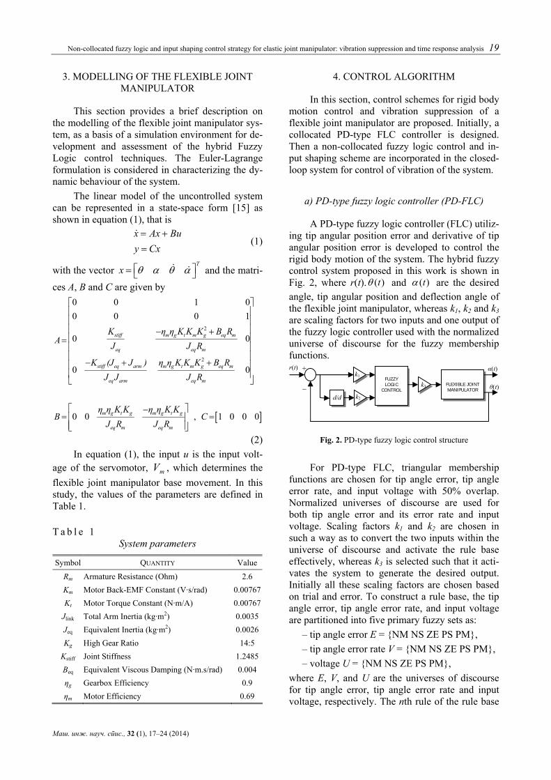
In this section, control schemes for rigid body motion control and vibration suppression of a flexible joint manipulator are proposed. Initially, a collocated PD-type FLC controller is designed. Then a non-collocated fuzzy logic control and in-put shaping scheme are incorporated in the closed-loop system for control of vibration of the system.
а) PD-type fuzzy logic controller (PD-FLC)
A PD-type fuzzy logic controller (FLC) utiliz-ing tip angular position error and derivative of tip angular position error is developed to control the rigid body motion of the system. The hybrid fuzzy control system proposed in this work is shown in Fig. 2, where r(t). )(tθ and )(tα are the desired angle, tip angular position and deflection angle of the flexible joint manipulator, whereas k1, k2 and k3 are scaling factors for two inputs and one output of the fuzzy logic controller used with the normalized universe of discourse for the fuzzy membership functions.
Fig. 2. PD-type fuzzy logic control structure
For PD-type FLC, triangular membership functions are chosen for tip angle error, tip angle error rate, and input voltage with 50% overlap. Normalized universes of discourse are used for both tip angle error and its error rate and input voltage. Scaling factors k1 and k2 are chosen in such a way as to convert the two inputs within the universe of discourse and activate the rule base effectively, whereas k3 is selected such that it acti-vates the system to generate the desired output. Initially all these scaling factors are chosen based on trial and error. To construct a rule base, the tip angle error, tip angle error rate, and input voltage are partitioned into five primary fuzzy sets as:
– tip angle error E = NM NS ZE PS PM, – tip angle error rate V = NM NS ZE PS PM, – voltage U = NM NS ZE PS PM,
where E, V, and U are the universes of discourse for tip angle error, tip angle error rate and input voltage, respectively. The nth rule of the rule base
FUZZY LOGIC
CONTROL
FLEXIBLE JOINT MANIPULATOR
k1
k2
k3
d/d
r(t) α(t)
θ(t)
+
_
20 M. Amin Rashidifar, A. Amin Rashidifar
Mech. Eng. Sci. J., 32 (1), 17–24 (2014)
for the FLC, with angle error and angle error rate as inputs, is given by
Rn: IF(e is Ei) AND (ė is Vj) THEN (u is Uk),
where Rn, n = 1, 2,…Nmax, is the nth fuzzy rule, Ei, Vj, and Uk, for i, j, k = 1, 2,…,5, are the primary fuzzy sets.
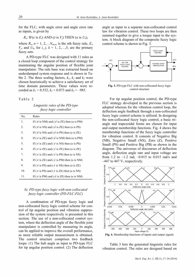
A PD-type FLC was designed with 11 rules as a closed loop component of the control strategy for maintaining the angular position of flexible joint manipulator. The rule base was extracted based on underdamped system response and is shown in Ta-ble 2. The three scaling factors, k1, k2 and k3 were chosen heuristically to achieve a satisfactory set of time domain parameters. These values were re-corded as k1 = 0.552, k2 = 0.073 and k3 = –985.
T a b l e 2
Linguistic rules of the PD-type fuzzy logic controller
No. Rules
1. If ( e is NM) and ( e is ZE) then (u is PM)
2. If ( e is NS) and ( e is ZE) then (u is PS)
3. If ( e is NS) and ( e is PS) then (u is ZE)
4. If ( e is ZE) and ( e is NM) then (u is PM)
5. If ( e is ZE) and ( e is NS) then (u is PS)
6. If ( e is ZE) and ( e is ZE) then (u is ZE)
7. If ( e is ZE) and ( e is PS) then (u is NS)
8. If ( e is ZE) and ( e is PM) then (u is NM)
9. If ( e is PS) and ( e is NS) then (u is ZE)
10. If ( e is PS) and ( e is ZE) then (u is NS)
11. If ( e is PM) and ( e is ZE) then (u is NM)
b). PD-type fuzzy logic with non-collocated fuzzy logic controller (PD-FLC-FLC)
A combination of PD-type fuzzy logic and non-collocated fuzzy logic control scheme for con-trol of tip angular position and vibration suppres-sion of the system respectively is presented in this section. The use of a non-collocated control sys-tem, where the deflection angle of the flexible joint manipulator is controlled by measuring its angle, can be applied to improve the overall performance, as more reliable output measurement is obtained. The control structure comprises two feedback loops: (1) The hub angle as input to PD-type FLC for tip angular position control. (2) The deflection
angle as input to a separate non-collocated control law for vibration control. These two loops are then summed together to give a torque input to the sys-tem. A block diagram of the composite fuzzy logic control scheme is shown in Fig. 3.
Fig. 3. PD-type FLC with non-collocated fuzzy logic control structure
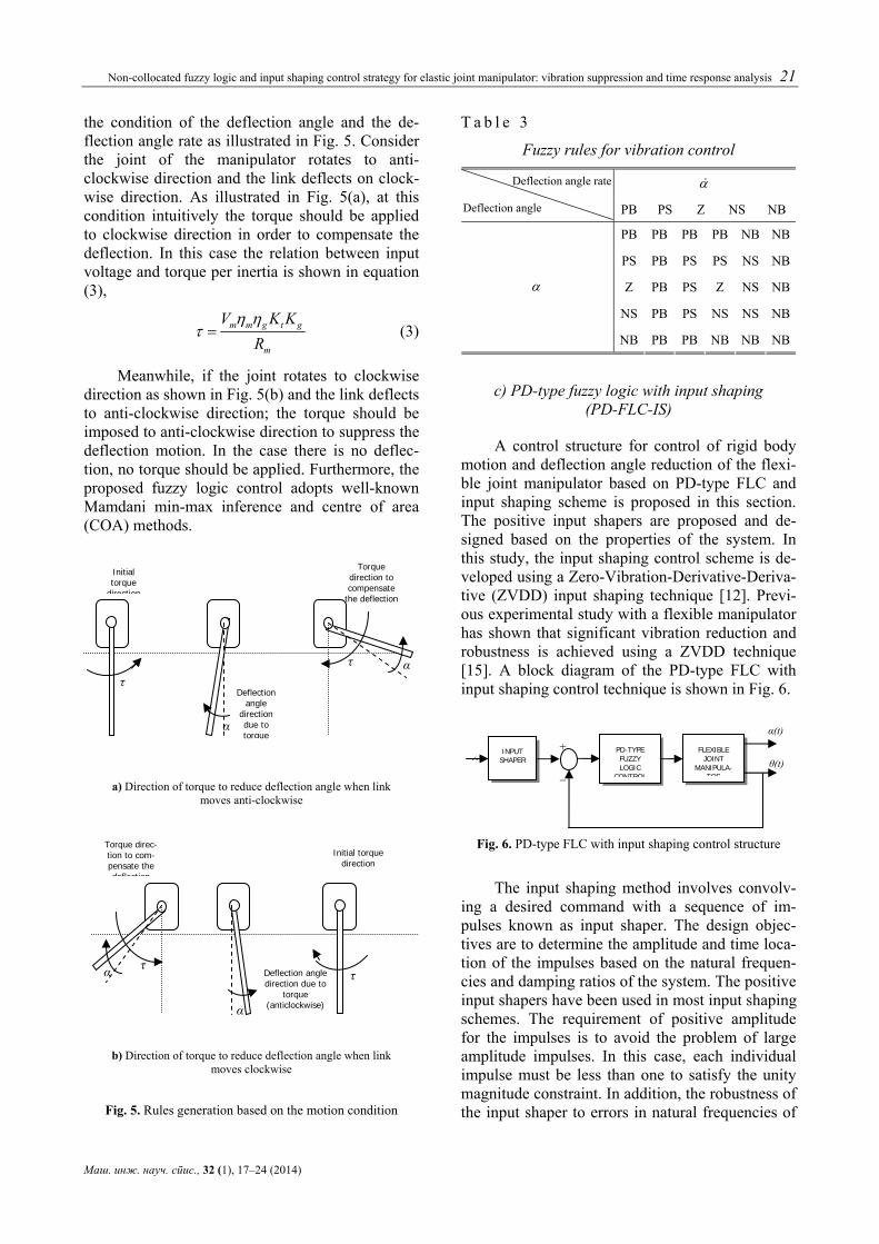
For tip angular position control, the PD-type FLC strategy developed in the previous section is adopted whereas for the vibration control loop, the deflection angle feedback through a non-collocated fuzzy logic control scheme is utilized. In designing the non-collocated fuzzy logic control, a basic tri-angle and trapezoidal forms are chosen for input and output membership functions. Fig. 4 shows the membership functions of the fuzzy logic controller for vibration control. It consists of Negative Big (NB), Negative Small (NS), Zero (Z), Positive Small (PS) and Positive Big (PB) as shown in the diagram. The universes of discourses of deflection angle, deflection angle rate and input voltage are from 1.2 to –1.2 rad, –0.015 to 0.015 rad/s and –447 to 447 V, respectively.
-400 -300 -200 -100 0 100 200 300 4000
0.5
1
Input voltage (V)
NB NS Z PS PB
Deg
ree
of m
embe
rshi
p
-0.015 -0.01 -0.005 0 0.005 0.01 0.0150
0.5
1
Deflection angle rate (rad/s)
Deg
ree
of m
embe
rshi
p
NB NS Z PS PB
1 0.8 0.6 0.4 0.2 0 -0.2 -0.4 -0.6 -0.8 -10
0.5
1
Deflection angle (rad)
NB NS Z PS PB
Deg
ree
of m
embe
rshi
p
Fig. 4. Membership functions of inputs and output signals
Table 3 lists the generated linguistic rules for vibration control. The rules are designed based on
PD-TYPE FUZZY LOGIC
CONTROL
FLEXIBLE JOINT MANIPULATOR
r(t) α(t)
θ(t)
+
_
_
+
FUZZY LOGIC CONTROL
Non-collocated fuzzy logic and input shaping control strategy for elastic joint manipulator: vibration suppression and time response analysis 21
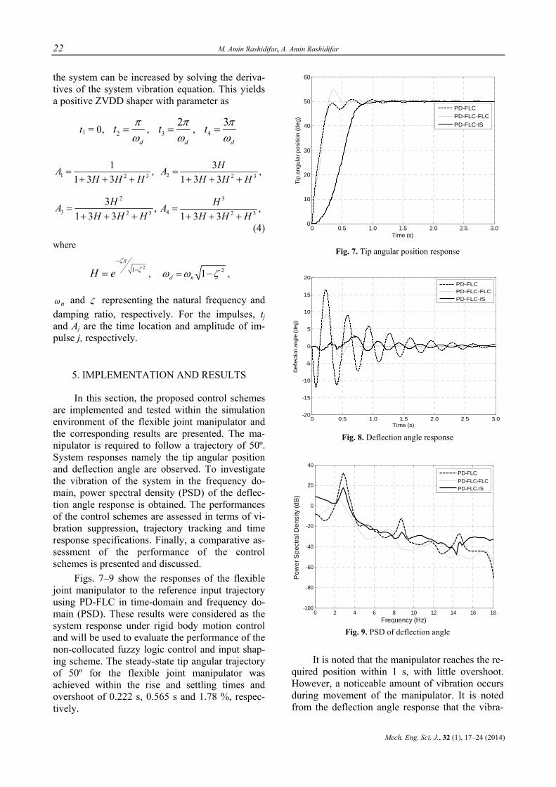
Маш. инж. науч. спис., 32 (1), 17–24 (2014)
the condition of the deflection angle and the de-flection angle rate as illustrated in Fig. 5. Consider the joint of the manipulator rotates to anti-clockwise direction and the link deflects on clock-wise direction. As illustrated in Fig. 5(a), at this condition intuitively the torque should be applied to clockwise direction in order to compensate the deflection. In this case the relation between input voltage and torque per inertia is shown in equation (3),
m m g t g
m
V K KR
η ητ = (3)
Meanwhile, if the joint rotates to clockwise direction as shown in Fig. 5(b) and the link deflects to anti-clockwise direction; the torque should be imposed to anti-clockwise direction to suppress the deflection motion. In the case there is no deflec-tion, no torque should be applied. Furthermore, the proposed fuzzy logic control adopts well-known Mamdani min-max inference and centre of area (COA) methods.
a) Direction of torque to reduce deflection angle when link
moves anti-clockwise
b) Direction of torque to reduce deflection angle when link moves clockwise
Fig. 5. Rules generation based on the motion condition
T a b l e 3
Fuzzy rules for vibration control
α Deflection angle rate
Deflection angle PB PS Z NS NB
PB PB PB PB NB NB
PS PB PS PS NS NB
Z PB PS Z NS NB
NS PB PS NS NS NB
α
NB PB PB NB NB NB
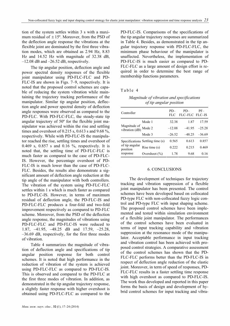
c) PD-type fuzzy logic with input shaping (PD-FLC-IS)
A control structure for control of rigid body motion and deflection angle reduction of the flexi-ble joint manipulator based on PD-type FLC and input shaping scheme is proposed in this section. The positive input shapers are proposed and de-signed based on the properties of the system. In this study, the input shaping control scheme is de-veloped using a Zero-Vibration-Derivative-Deriva-tive (ZVDD) input shaping technique [12]. Previ-ous experimental study with a flexible manipulator has shown that significant vibration reduction and robustness is achieved using a ZVDD technique [15]. A block diagram of the PD-type FLC with input shaping control technique is shown in Fig. 6.
Fig. 6. PD-type FLC with input shaping control structure
The input shaping method involves convolv-ing a desired command with a sequence of im-pulses known as input shaper. The design objec-tives are to determine the amplitude and time loca-tion of the impulses based on the natural frequen-cies and damping ratios of the system. The positive input shapers have been used in most input shaping schemes. The requirement of positive amplitude for the impulses is to avoid the problem of large amplitude impulses. In this case, each individual impulse must be less than one to satisfy the unity magnitude constraint. In addition, the robustness of the input shaper to errors in natural frequencies of
Initial torque
direction
Deflection angle
direction due to torque
Torque direction to compensate
the deflection
τ τ α
Initial torque direction
Deflection angle direction due to
torque (anticlockwise)
Torque direc-tion to com-pensate the deflection
α
τ τ α
PD-TYPE FUZZY LOGIC
CONTROL
FLEXIBLE JOINT
MANIPULA-TOR
(t)
α(t)
θ(t)
INPUT SHAPER
+
_
α
22 M. Amin Rashidifar, A. Amin Rashidifar
Mech. Eng. Sci. J., 32 (1), 17–24 (2014)
the system can be increased by solving the deriva-tives of the system vibration equation. This yields a positive ZVDD shaper with parameter as
t1 = 0, 2d
t πω
= , 32
d
t πω
= , 43
d
t πω
=
1 2 3
1 ,1 3 3
AH H H
=+ + +
2 2 3
3 ,1 3 3
HAH H H
=+ + +
2
3 2 3
3 ,1 3 3
HAH H H
=+ + +
3
4 2 3 ,1 3 3
HAH H H
=+ + +
(4) where
21H e
ζπζ
−−= , 21d nω ω ζ= − ,
nω and ζ representing the natural frequency and damping ratio, respectively. For the impulses, tj and Aj are the time location and amplitude of im-pulse j, respectively.
5. IMPLEMENTATION AND RESULTS
In this section, the proposed control schemes are implemented and tested within the simulation environment of the flexible joint manipulator and the corresponding results are presented. The ma-nipulator is required to follow a trajectory of 50º. System responses namely the tip angular position and deflection angle are observed. To investigate the vibration of the system in the frequency do-main, power spectral density (PSD) of the deflec-tion angle response is obtained. The performances of the control schemes are assessed in terms of vi-bration suppression, trajectory tracking and time response specifications. Finally, a comparative as-sessment of the performance of the control schemes is presented and discussed.
Figs. 7–9 show the responses of the flexible joint manipulator to the reference input trajectory using PD-FLC in time-domain and frequency do-main (PSD). These results were considered as the system response under rigid body motion control and will be used to evaluate the performance of the non-collocated fuzzy logic control and input shap-ing scheme. The steady-state tip angular trajectory of 50º for the flexible joint manipulator was achieved within the rise and settling times and overshoot of 0.222 s, 0.565 s and 1.78 %, respec-tively.
0 0.5 1.0 1.5 2.0 2.5 3.00
10
20
30
40
50
60
Time (s)
Tip
angu
lar p
ositi
on (d
eg)
PD-FLCPD-FLC-FLCPD-FLC-IS
Fig. 7. Tip angular position response
0 0.5 1.0 1.5 2.0 2.5 3.0-20
-15
-10
-5
0
5
10
15
20
Time (s)
Def
lect
ion
angl
e (d
eg)
PD-FLCPD-FLC-FLCPD-FLC-IS
Fig. 8. Deflection angle response
0 2 4 6 8 10 12 14 16 18-100
-80
-60
-40
-20
0
20
40
Frequency (Hz)
Pow
er S
pect
ral D
ensi
ty (d
B)
PD-FLCPD-FLC-FLCPD-FLC-IS
Fig. 9. PSD of deflection angle
It is noted that the manipulator reaches the re-quired position within 1 s, with little overshoot. However, a noticeable amount of vibration occurs during movement of the manipulator. It is noted from the deflection angle response that the vibra-
Non-collocated fuzzy logic and input shaping control strategy for elastic joint manipulator: vibration suppression and time response analysis 23
Маш. инж. науч. спис., 32 (1), 17–24 (2014)
tion of the system settles within 3 s with a maxi-mum residual of ± 15º. Moreover, from the PSD of the deflection angle response the vibrations at the flexible joint are dominated by the first three vibra-tion modes, which are obtained as 2.94 Hz, 8.83 Hz and 14.52 Hz with magnitude of 32.38 dB, –12.08 dB and –26.52 dB, respectively.
The tip angular position, deflection angle and power spectral density responses of the flexible joint manipulator using PD-FLC-FLC and PD-FLC-IS are shown in Figs. 7–9, respectively. It is noted that the proposed control schemes are capa-ble of reducing the system vibration while main-taining the trajectory tracking performance of the manipulator. Similar tip angular position, deflec-tion angle and power spectral density of deflection angle responses were observed as compared to the PD-FLC. With PD-FLC-FLC, the steady-state tip angular trajectory of 50º for the flexible joint ma-nipulator was achieved within the rise and settling times and overshoot of 0.215 s, 0.613 s and 9.68 %, respectively. While with PD-FLC-IS the manipula-tor reached the rise, settling times and overshoot of 0.469 s, 0.857 s and 0.16 %, respectively. It is noted that, the settling time of PD-FLC-FLC is much faster as compared to the case of PD-FLC-IS. However, the percentage overshoot of PD-FLC-IS is much lower than the case of PD-FLC-FLC. Besides, the results also demonstrate a sig-nificant amount of deflection angle reduction at the tip angle of the manipulator with both controllers. The vibration of the system using PD-FLC-FLC settles within 1 s which is much faster as compared to PD-FLC-IS. However, in terms of maximum residual of deflection angle, the PD-FLC-IS and PD-FLC-FLC produces a four-fold and two-fold improvement respectively as compared to PD-FLC scheme. Moreover, from the PSD of the deflection angle response, the magnitudes of vibrations using PD-FLC-FLC and PD-FLC-IS were reduced to 1.87, –41.95, –48.25 dB and 17.59, –25.28, –36.69 dB, respectively, for the first three modes of vibration.
Table 4 summarizes the magnitude of vibra-tion of deflection angle and specifications of tip angular position response for both control schemes. It is noted that high performance in the reduction of vibration of the system is achieved using PD-FLC-FLC as compared to PD-FLC-IS. This is observed and compared to the PD-FLC at the first three modes of vibration. In addition, as demonstrated in the tip angular trajectory response, a slightly faster response with higher overshoot is obtained using PD-FLC-FLC as compared to the
PD-FLC-IS. Comparisons of the specifications of the tip angular trajectory responses are summarized in Table 4. Besides, as demonstrated in the tip an-gular trajectory response with PD-FLC-FLC, the minimum phase behaviour of the manipulator is unaffected. Nevertheless, the implementation of PD-FLC-IS is much easier as compared to PD-FLC-FLC as a large amount of design effort is re-quired in order to determine the best range of membership functions parameters.
T a b l e 4
Magnitude of vibration and specifications of tip angular position
Controller PD–FLC
PD– FLC–FLC
PF–FLC–IS
Mode 1 32.38 1.87 17.59
Mode 2 –12.08 –41.95 –25.28Magnitude of vibration (dB)
Mode 3 –26.52 –48.25 –36.69
Settling time (s) 0.565 0.613 0.857
Rise time (s) 0.222 0.215 0.469
Specifications of tip angular position response Overshoot (%) 1.78 9.68 0.16
6. CONCLUSIONS
The development of techniques for trajectory tracking and vibration suppression of a flexible joint manipulator has been presented. The control schemes have been developed based on collocated PD-type FLC with non-collocated fuzzy logic con-trol and PD-type FLC with input shaping scheme. The proposed control schemes have been imple-mented and tested within simulation environment of a flexible joint manipulator. The performances of the control schemes have been evaluated in terms of input tracking capability and vibration suppression at the resonance mode of the manipu-lator. Acceptable performance in input tracking and vibration control has been achieved with pro-posed control strategies. A comparative assessment of the control schemes has shown that the PD-FLC-FLC performs better than the PD-FLC-IS in respect of deflection angle reduction of the elastic joint. Moreover, in term of speed of responses, PD-FLC-FLC results in a faster settling time response with high overshoot as compared to PD-FLC-IS. The work thus developed and reported in this paper forms the basis of design and development of hy-brid control schemes for input tracking and vibra-
24 M. Amin Rashidifar, A. Amin Rashidifar
Mech. Eng. Sci. J., 32 (1), 17–24 (2014)
tion suppression of multi-link flexible manipulator systems and can be extended to and adopted in practical applications.
REFERENCES
[1] Yim, W.: Adaptive Control of a Flexible Joint Manipula-tor. Proc. 2001 IEEE, International Robotics & Automa-tion, Seoul, Korea, pp. 3441–3446 (2001).
[2] Oh, J. H. and Lee, J. S.: Control of Flexible Joint Robot System by Backstepping Design Approach. Proc. of IEEE International Conference on Robotics & Automation, pp. 3435–3440 (1997).
[3] Ghorbel, F., Hung, J. Y. and Spong, M. W.: Adaptive Control of Flexible Joint Manipulators. Control Systems Magazine, Vol. 9, pp. 9–13 (1989).
[4] Lin, L. C. and Yuan, K.: Control of Flexible Joint Robots via External Linearization Approach. Journal of Robotic Systems, 1 (1), 1–22 (2007).
[5] Spong, M. W., Khorasani, K. and Kokotovic, P. V.: An Integral Manifold Approach to the Feedback Control of Flexible Joint Robots. IEEE Journal of Robotics and Automation, Vol. RA-3, No. 4, pp. 291–300 (1987).
[6] Tomei, P.: A Simple PD Controller for Robots with Elas-tic Joints. IEEE Trans. on Automatic Control, Vol. 36, No. 10, pp. 1208–1213 (1991).
[7] Yeon, J. S. and Park, J. H.: Practical Robust Control for Flexible Joint Robot Manipulators. Proc. 2008 IEEE In-ternational Conference on Robotic and Automation, Pasadena, CA, USA, pp. 3377–3382 (2008).
[8] Ahmad, M. A.: Vibration and Input Tracking Control of Flexible Manipulator Using LQR with Non-collocated PID Controller. Proc. of 2nd UKSIM European Sympo-sium on Computer Modelling and Simulation, Liverpool, United Kingdom, pp. 40–45 (2008).
[9] Tokhi, M. O. and Azad, A. K. M.: Control of flexible manipulator systems. Proceedings IMechE-I: Journal of Systems and Control Engineering, 210, 113–130 (1996).
[10] Ahmad, M. A., Nasir, A. N. K., Hambali, N. and Ishak, H.: Vibration and Input Tracking Control of Flexible Ma-nipulator Using Hybrid Fuzzy Logic Controller. Proceed-ings of the IEEE International Conference of Mechatron-ics and Automation, Kagawa, Jepun, pp. 593–598 (2008).
[11] Shchuka, A. and Goldenberg, A. A.: Tip control of a sin-gle-link flexible arm using feedforward technique. Me-chanical Machine Theory, 24, pp. 439–455 (1989).
[12] Mohamed, Z. and Ahmad, M. A.: Hybrid Input Shaping and Feedback Control Schemes of a Flexible Robot Ma-nipulator. Proceedings of the 17th World Congress the In-ternational Federation of Automatic Control, Seoul, Ko-rea, pp. 11714–11719 (2008).
[13] Rattan, K. S., Feliu, V. and Brown, H. B.: Tip position control of flexible arms. Proceedings of the IEEE Confer-ence on Decision and Control, Honolulu, pp. 1803–1808 (1990).
[14] Quanser Student Handout, Rotary Flexible Joint Module. http://www.quanser.com.
[15] Mohamed, Z. and Tokhi, M. O.: Vibration control of a single-link flexible manipulator using command shaping techniques. Proceedings IMechE-I: Journal of Systems and Control Engineering, 216, pp. 191–210 (2002).
Mechanical Engineering – Scientific Journal, Vol. 32, No. 1, pp. 25–33 (2014) CODEN: MINSC5 – 450 In print: ISSN 1857–5293 Received: March 19, 2014 On line: ISSN 1857–9191 Accepted: April 20, 2014 UDC: 629.33./27.484–59
Original scientific paper
STRUCTURAL AND CONTACT ANALYSIS OF DISC BRAKE ASSEMBLY DURING SINGLE STOP BRAKING EVENT
Ali Belhocine1, Abd Rahim Abu Bakar2, Mostefa Bouchetara3 1,3Institute of Mechanical Engineering, Faculty of Mechanical Engineering,
University of Sciences and the Technology of Oran, L.P 1505 El - Mnaouer, USTO 31000 Oran (Algeria)
2Department of Automotive Engineering, Universiti Teknologi Malaysia, 81310 UTM Skudai (Malaysia).
[email protected] // [email protected]
A b s t r a c t: An automobile disc brake system is used to perform three basic functions, i.e. to reduce speed of a vehicle, to maintain its speed when travelling downhill and to completely stop the vehicle. During these braking events, the disc brake may suffer of structural and wear issues. It is quite sometimes that the disc brake components fail structurally and/or having severe wear on the pad. Thus, this paper aims to examine stress concentration, struc-tural deformation and contact pressure of brake disc and pads during single braking stop event by employing com-mercial finite element software, ANSYS. The paper also highlights the effects of using a fixed calliper, different fric-tion coefficients and different speeds of the disc on the stress concentration, structural deformation and contact pres-sure of brake disc and pads, respectively.
Key words: disc brake; Von Mises stress; structural deformation; contact pressure; finite element
СТРУКТУРНА И КОНТАКТНА АНАЛИЗА НА СКЛОП НА КОЧНИЦИ СО ДИСКОВИ ЗА ВРЕМЕ НА ЕДИНИЧНО СOПИРАЊЕ
А п с т р а к т: Систем за кочење кај автомобилите има 3 основни функции: да ја намали брзината на возилото, да ја одржи брзината кога возилото се движи по удолница и целосно да го запре возилото. За време на кочење дисковите можат да трпат структурни проблеми или проблеми од замор на материјалот. Често се случува компоненти на системот за кочење да откажат поради промена на структурата или површината на материјалот. Овој труд е посветен на истражувања на концентрација на напон, деформации и притисок на до-пир на дисковите за време на единично сопирање со употреба на комерцијален софтвер за метод на конечни елементи, АНСЅС. Трудот исто така се фокусира на ефектот на користење фиксен носач на плочките, разли-чни фрикциони коефициенти и различни брзини на дискот врз концентрацијата на напони, деформацијата и притисокот на допир на дисковите и плочките, соодветно.
Клучни зборови: диск за кочење; Von Mises-ов напон; деформација; притисок на допир; конечен елемент
1. INTRODUCTION
Passenger car disc brakes are safety-critical components whose performance depends strongly on the contact conditions at the pad-to-rotor inter-face. When the driver steps on the brake pedal, hydraulic fluid is pushed against the piston, which in turn forces the brake pads into contact with the
rotor. The frictional forces at the sliding interfaces between the pads and the rotor retard the rotational movement of the rotor and the axle on which it is mounted [1]. The kinetic energy of the vehicle is transformed into heat that is mainly absorbed by the rotor and the brake pad.
The frictional heat generated on the interface of the disc and the pads can cause high tempera-

26 A. Belhocine, A. Rahim Abu Bakar, M. Bouchetara
Mech. Eng. Sci. J., 32 (1), 25–33 (2014)
ture. Particularly, the temperature may exceed the critical value for a given material, which leads to undesirable effects, such as brake fade, local scor-ing, thermo elastic instability, premature wear, brake fluid vaporization, bearing failure, thermal cracks, and thermally excited vibration [2, 3]. Gao and Lin [2] stated that there was considerable evi-dence to show that the contact temperature is an integral factor reflecting the specific power friction influence of combined effect of load, speed, fric-tion coefficient, and the thermo physical and dura-bility properties of the materials of a frictional couple. Lee and Yeo [3] reported that uneven dis-tribution of temperature at the surfaces of the disc and friction pads brings about thermal distortion, which is known as coning and found to be the main cause of judder and disc thickness variation (DTV). AbuBakar et al. [4] in their recent work found that temperature could also affect vibration level in a disc brake assembly. Valvano and Lee [5] simulated thermal analysis on a disc brake with a combination of computer-based thermal model and finite element-based techniques to provide a reliable method to calculate the temperature rise, thermal stress and distortion under a given brake schedule. Wolejsza et al. [6] performed analysis on the thermo-mechanical behavior of airplane carbon composite brakes using MSC/Marc finite element software which allows accurate simulation of the transient heat transfer phenomenon coupled to disc deformations caused by frictional sliding contact.
There are three types of mechanical stresses subjected by the disc brake. The first one is the traction force created by the centrifugal effect due to the rotational of the disc brake when the wheel is rotating and no braking force is applied to the disc. During braking operation, there are another two additional forces experienced by the disc brake. Firstly, compression force is created as the result of the force exerted by the brake pad press-ing perpendicular onto the surface of the disc to slow it down. Secondly, the braking action due to the rubbing of the brake pad against the surface of the disc brake is translated into frictional or trac-tion force on the disc surface which acts in the op-posite direction of the disc rotation.
A disc brake of floating caliper design typi-cally consists of pads, caliper, carrier, rotor (disc), piston, and guide pins. One of the major require-ments of the caliper is to press the pads against the rotor and should ideally achieve as uniform inter-face pressure as possible. A uniform pressure be-tween the pads and rotor leads to uniform pad wear
and brake temperature, and more even friction co-efficients [7]. Unevenness of the pressure distribu-tion could cause uneven wear and shorter life of pads. It has also speculated that they may promote disc brake squeal. The interface pressure distribu-tions have been investigated by a number of peo-ple. Tirovic and Day [8] studied the influence of component geometry, material properties and con-tact characteristics on the interface pressure distri-bution. Belhocine and Bouchetara [9] recently studied the interface pressure distributions of the inner pad under the influence of the thermome-chanical coupling in the braking process. They used a simple and nonvalidated, three-dimensional model of the disc brake. Tamari et al. [10] pre-sented a method of predicting disc brake pad con-tact pressure for certain operating condition by means of experimental and numerical method. They developed a quite detailed model and vali-dated the model by fitting the numerical deforma-tions of the disc brake components with experi-mental results. Hohmann et al. [11] also presented a method of contact analysis for the drum and disc brakes of simple three-dimensional models using ADINA software package. They showed a sticking and shifting contact area in their results. Like [8], validation of their model was not made. Ripin [12] developed a simple, validated three-dimensional finite element model of the pad, and applied rather simple piston and finger force onto the back plate interface in his analysis. He studied the contact pressure distribution at the disc/pad interface, where gap elements were used to represent contact effect.
In this paper, structural analysis is performed on a simple finite element (FE) model of a real disc brake assembly to obtain the contact pressure dis-tributions on the friction pads and the Von Mises Stress in disc interface by utilizing the ANSYS 11.0 FE software. Sensitivity study on rotation of the disc, load pattern and coefficient of friction is also performed.
2. INITER ELEMENT ANALYSIS
In this work, a three dimensional CAD and FE model consists of a ventilated disc and two pads with single slot in the middle as illustrated in Fig. 1 and Fig. 2, respectively. The selected mate-rial of the disc is Gray cast iron FG 15 with high Carbon content and the brake pad has an isotropic elastic behavior whose mechanical characteristics of the two parts are presented in Table 1. The ma-

Structural and contact analysis of disc brake assembly during single stop braking event 27
Маш. инж. науч. спис., 32 (1), 25–33 (2014)
terials of the disc and the pads are homogeneous and their properties are invariable with the tem-perature.
T a b l e 1 Mechanical properties of the disc and pad
Properties Disc Pad
Young modulus E (GPa) 138 1
Poisson's ratio ν 0.3 0.25
Density ρ (kg/m3) 7250 1400
Coefficient of friction µ 0.2 0.2
Fig. 1. CAD model of the disc and pads
Fig. 2. FE model of the disc and pads
A commercial FE software, namely ANSYS 11 (3D) is fully utilised to simulate structural de-formation and contact pressure distributions of the disc brake during single braking stop application. Boundary conditions are imposed on the models (disc-pad) as shown in Fig. 3a for applied pressure
on one side of the pad and Fig. 3b for applied pres-sure on both sides of the pad. The disc is rigidly constrained at the bolt holes in all directions except in its rotational direction. Meanwhile, the pad is fixed at the abutment in all degrees of freedom ex-cept in the normal direction to allow the pads move up and down and in contact with the disc surface. In this study, it is assumed that 60% of the braking forces are supported by the front brakes (two ro-tors) [13]. By using vehicle data as given in Table 2 and Eqs. (1) – (3), braking force on the disc, rota-tional speed and brake pressure on the pad can be calculated, respectively.
a) One side
(b) Two sides
Fig. 3 Boundary conditions and loading imposed on the disc-pads
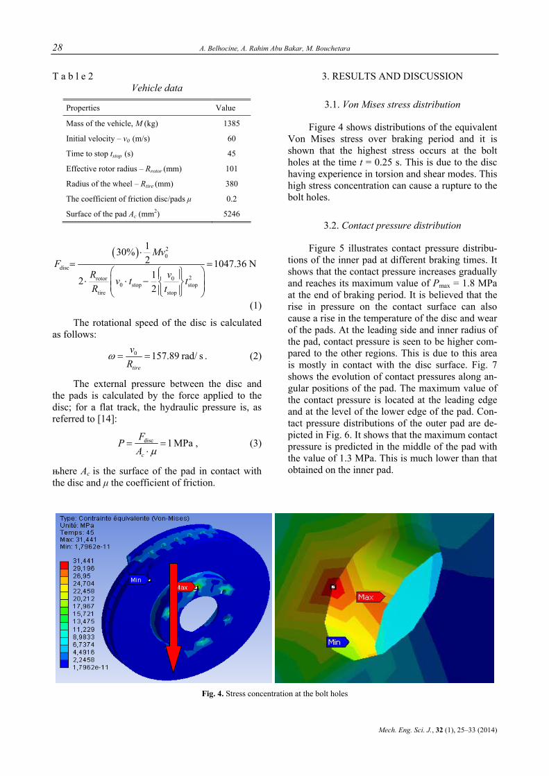
28 A. Belhocine, A. Rahim Abu Bakar, M. Bouchetara
Mech. Eng. Sci. J., 32 (1), 25–33 (2014)
T a b l e 2 Vehicle data
Properties Value
Mass of the vehicle, M (kg) 1385
Initial velocity – v0 (m/s) 60
Time to stop tstop (s) 45
Effective rotor radius – Rrotor (mm) 101
Radius of the wheel – Rtire (mm) 380
The coefficient of friction disc/pads µ 0.2
Surface of the pad Ac (mm2) 5246
( ) 20
disc
2rotor 00 stop stop
tire stop
130%2 1047.36 N
122
MvF
R vv t tR t
⋅= =
⎛ ⎞⎧ ⎫⎪ ⎪⋅ ⋅ −⎜ ⎟⎨ ⎬⎜ ⎟⎪ ⎪⎩ ⎭⎝ ⎠
(1)
The rotational speed of the disc is calculated as follows:
0 157.89 rad/ stire
vR
ω = = . (2)
The external pressure between the disc and the pads is calculated by the force applied to the disc; for a flat track, the hydraulic pressure is, as referred to [14]:
disc 1 MPac
FPA µ
= =⋅
, (3)
њhere Ac is the surface of the pad in contact with the disc and µ the coefficient of friction.
3. RESULTS AND DISCUSSION
3.1. Von Mises stress distribution
Figure 4 shows distributions of the equivalent Von Mises stress over braking period and it is shown that the highest stress occurs at the bolt holes at the time t = 0.25 s. This is due to the disc having experience in torsion and shear modes. This high stress concentration can cause a rupture to the bolt holes.
3.2. Contact pressure distribution
Figure 5 illustrates contact pressure distribu-tions of the inner pad at different braking times. It shows that the contact pressure increases gradually and reaches its maximum value of Pmax = 1.8 MPa at the end of braking period. It is believed that the rise in pressure on the contact surface can also cause a rise in the temperature of the disc and wear of the pads. At the leading side and inner radius of the pad, contact pressure is seen to be higher com-pared to the other regions. This is due to this area is mostly in contact with the disc surface. Fig. 7 shows the evolution of contact pressures along an-gular positions of the pad. The maximum value of the contact pressure is located at the leading edge and at the level of the lower edge of the pad. Con-tact pressure distributions of the outer pad are de-picted in Fig. 6. It shows that the maximum contact pressure is predicted in the middle of the pad with the value of 1.3 MPa. This is much lower than that obtained on the inner pad.
Fig. 4. Stress concentration at the bolt holes

Structural and contact analysis of disc brake assembly during single stop braking event 29
Маш. инж. науч. спис., 32 (1), 25–33 (2014)
a) at time t = 0.25 s
e) at time t = 2.5 s
b) at time t = 0.5 s
f) at time t = 3 s
c) at time t = 1 s
g) at time t = 3.5 s
d) at time t =2 s
h) at time t = 45 s
Fig. 5. Contact pressure distribution on the inner pad
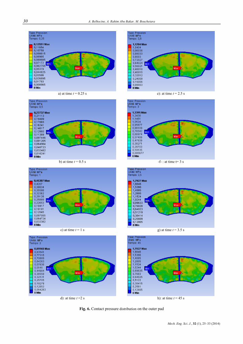
30 A. Belhocine, A. Rahim Abu Bakar, M. Bouchetara
Mech. Eng. Sci. J., 32 (1), 25–33 (2014)
a) at time t = 0.25 s
e): at time t = 2.5 s
b) at time t = 0.5 s
-f- : at time t= 3 s
c) at time t = 1 s
g) at time t = 3.5 s
d): at time t =2 s
h): at time t = 45 s
Fig. 6. Contact pressure distribution on the outer pad
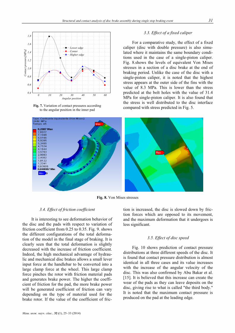
Structural and contact analysis of disc brake assembly during single stop braking event 31
Маш. инж. науч. спис., 32 (1), 25–33 (2014)
0 10 20 30 40 50 60
0,4
0,6
0,8
1,0
1,2
1,4
1,6
1,8
Con
tact
pre
ssur
e[M
Pa]
Angular position
Lower edge Center Higher edge
Fig. 7. Variation of contact pressures according
to the angular position in the inner pad
3.3. Effect of a fixed caliper
For a comparative study, the effect of a fixed caliper (disc with double pressure) is also simu-lated where it maintains the same boundary condi-tions used in the case of a single-piston caliper. Fig. 8.shows the levels of equivalent Von Mises stresses in a section of a disc brake at the end of braking period. Unlike the case of the disc with a single-piston caliper, it is noted that the highest stress appears at the outer side of the fins with the value of 8.3 MPa. This is lower than the stress predicted at the bolt holes with the value of 31.4 MPa for single-piston caliper. It is also found that the stress is well distributed to the disc interface compared with stress predicted in Fig. 5.
Fig. 8. Von Mises stresses
3.4. Effect of friction coefficient
It is interesting to see deformation behavior of the disc and the pads with respect to variation of friction coefficient from 0.25 to 0.35. Fig. 9. shows the different configurations of the total deforma-tion of the model in the final stage of braking. It is clearly seen that the total deformation is slightly decreased with the increase of friction coefficient. Indeed, the high mechanical advantage of hydrau-lic and mechanical disc brakes allows a small lever input force at the handlebar to be converted into a large clamp force at the wheel. This large clamp force pinches the rotor with friction material pads and generates brake power. The higher the coeffi-cient of friction for the pad, the more brake power will be generated coefficient of friction can vary depending on the type of material used for the brake rotor. If the value of the coefficient of fric-
tion is increased, the disc is slowed down by fric-tion forces which are opposed to its movement, and the maximum deformation that it undergoes is less significant.
3.5. Effect of disc speed
Fig. 10 shows prediction of contact pressure distributions at three different speeds of the disc. It is found that contact pressure distribution is almost identical in all three cases and its value increases with the increase of the angular velocity of the disc. This was also confirmed by Abu Bakar et al. [15]. It is believed that this increase can create the wear of the pads as they can leave deposits on the disc, giving rise to what is called "the third body." It is noted that the maximum contact pressure is produced on the pad at the leading edge.
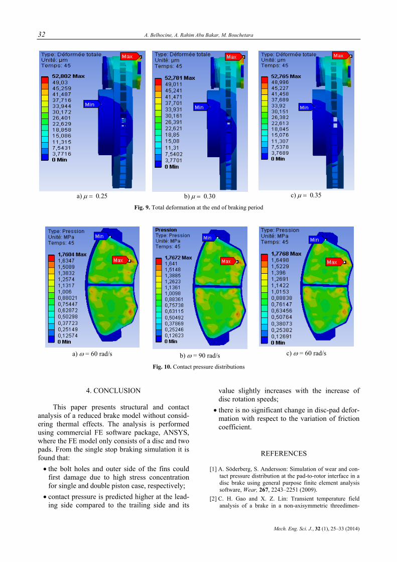
32 A. Belhocine, A. Rahim Abu Bakar, M. Bouchetara
Mech. Eng. Sci. J., 32 (1), 25–33 (2014)
a) µ = 0.25
b) µ = 0.30
c) µ = 0.35
Fig. 9. Total deformation at the end of braking period
a) ω = 60 rad/s
b) ω = 90 rad/s
c) ω = 60 rad/s
Fig. 10. Contact pressure distributions
4. CONCLUSION
This paper presents structural and contact analysis of a reduced brake model without consid-ering thermal effects. The analysis is performed using commercial FE software package, ANSYS, where the FE model only consists of a disc and two pads. From the single stop braking simulation it is found that:
• the bolt holes and outer side of the fins could first damage due to high stress concentration for single and double piston case, respectively;
• contact pressure is predicted higher at the lead-ing side compared to the trailing side and its
value slightly increases with the increase of disc rotation speeds;
• there is no significant change in disc-pad defor-mation with respect to the variation of friction coefficient.
REFERENCES
[1] A. Söderberg, S. Andersson: Simulation of wear and con-tact pressure distribution at the pad-to-rotor interface in a disc brake using general purpose finite element analysis software, Wear, 267, 2243–2251 (2009).
[2] C. H. Gao and X. Z. Lin: Transient temperature field analysis of a brake in a non-axisymmetric threedimen-
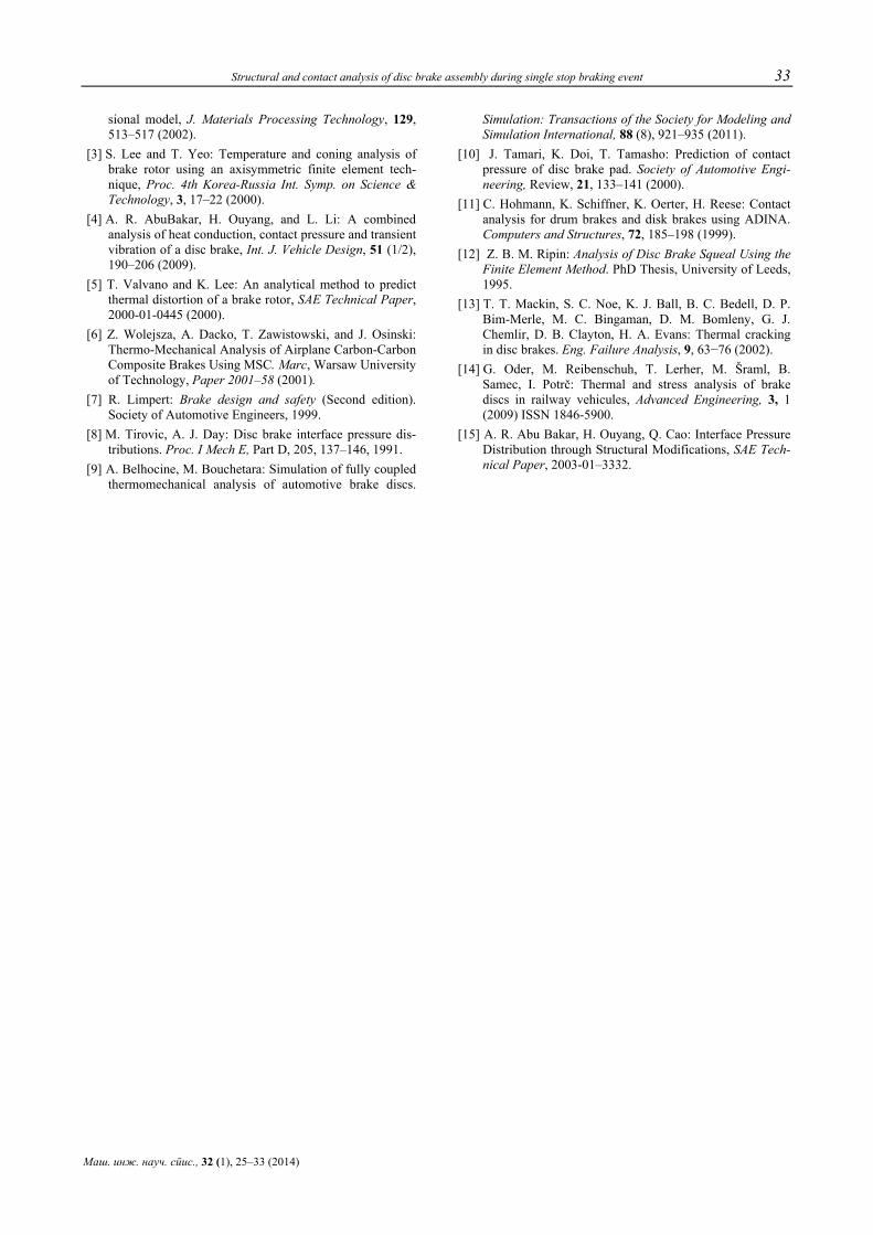
Structural and contact analysis of disc brake assembly during single stop braking event 33
Маш. инж. науч. спис., 32 (1), 25–33 (2014)
sional model, J. Materials Processing Technology, 129, 513–517 (2002).
[3] S. Lee and T. Yeo: Temperature and coning analysis of brake rotor using an axisymmetric finite element tech-nique, Proc. 4th Korea-Russia Int. Symp. on Science & Technology, 3, 17–22 (2000).
[4] A. R. AbuBakar, H. Ouyang, and L. Li: A combined analysis of heat conduction, contact pressure and transient vibration of a disc brake, Int. J. Vehicle Design, 51 (1/2), 190–206 (2009).
[5] T. Valvano and K. Lee: An analytical method to predict thermal distortion of a brake rotor, SAE Technical Paper, 2000-01-0445 (2000).
[6] Z. Wolejsza, A. Dacko, T. Zawistowski, and J. Osinski: Thermo-Mechanical Analysis of Airplane Carbon-Carbon Composite Brakes Using MSC. Marc, Warsaw University of Technology, Paper 2001–58 (2001).
[7] R. Limpert: Brake design and safety (Second edition). Society of Automotive Engineers, 1999.
[8] M. Tirovic, A. J. Day: Disc brake interface pressure dis-tributions. Proc. I Mech E, Part D, 205, 137–146, 1991.
[9] A. Belhocine, M. Bouchetara: Simulation of fully coupled thermomechanical analysis of automotive brake discs.
Simulation: Transactions of the Society for Modeling and Simulation International, 88 (8), 921–935 (2011).
[10] J. Tamari, K. Doi, T. Tamasho: Prediction of contact pressure of disc brake pad. Society of Automotive Engi-neering, Review, 21, 133–141 (2000).
[11] C. Hohmann, K. Schiffner, K. Oerter, H. Reese: Contact analysis for drum brakes and disk brakes using ADINA. Computers and Structures, 72, 185–198 (1999).
[12] Z. B. M. Ripin: Analysis of Disc Brake Squeal Using the Finite Element Method. PhD Thesis, University of Leeds, 1995.
[13] T. T. Mackin, S. C. Noe, K. J. Ball, B. C. Bedell, D. P. Bim-Merle, M. C. Bingaman, D. M. Bomleny, G. J. Chemlir, D. B. Clayton, H. A. Evans: Thermal cracking in disc brakes. Eng. Failure Analysis, 9, 63−76 (2002).
[14] G. Oder, M. Reibenschuh, T. Lerher, M. Šraml, B. Samec, I. Potrč: Thermal and stress analysis of brake discs in railway vehicules, Advanced Engineering, 3, 1 (2009) ISSN 1846-5900.
[15] A. R. Abu Bakar, H. Ouyang, Q. Cao: Interface Pressure Distribution through Structural Modifications, SAE Tech-nical Paper, 2003-01–3332.

Mechanical Engineering – Scientific Journal, Vol. 32, No. 1, pp. 35–44 (2014) CODEN: MINSC5 – 451 In print: ISSN 1857–5293 Received: March 3, 2014 On line: ISSN 1857–9191 Accepted: April 20, 2014 UDC: 662.767:504.5–044.245
Original scientific paper
USE OF NATURAL GAS AS A CONTRIBUTION TO REDUCING EMISSIONS
Dame Dimitrovski1, Goran Dimeski2 1"Ss. Cyril and Methodius" University in Skopje, Faculty of Mechanical Engineering,
Karpoš II. bb, P.O. box 464, 1001 Skopje, Republic of Macedonia 2Toplifikacija Inženering AD, 1000 Skopje, Republic of Macedonia
A b s t r a c t: Air quality is one of the conditions that affect both humans health also extend to natural ecosys-tems, stratospheric ozone, biosphere, changing weather conditions and climate. Imbalance in the atmosphere, the ap-pearance of the greenhouse effect, as well as damage the ozone layer is due to the release of large amounts of pollut-ing substances, which give the effect of acidification and ruin the biosphere, soil and affect others. Pollutants emitted into the air from various sources, mix it, and transported on greater distances and affect on air quality. The polluting substances emitted and remain part of the troposphere that is one part of the air that people breathe, with negative ef-fect on human health, especially respiratory. Given the rapid growth of the industry and the growing need for energy, it is necessary to consider the possibilities for the application of alternative fuels as a proposal to reduce emissions. This paper is considered part of the urban area and thus created a comparative analysis of the work of one plant (which is mainly supplying the area with heat energy), in terms of the type of fuel and related emissions. Also con-sider the possibility and benefits of the use of natural gas as an alternative fuel to meet the needs of households. Pre-pared analysis is presented also with the benefits of replacing the electrical and thermal energy (taken from the dis-trict heating system) with the use of natural gas as energy terms, and the financial and environmental.
Key words: pollutions; emissions; energy; natural gas
УПОТРЕБА НА ПРИРОДЕН ГАС КАКО ПРИДОНЕС ЗА НАМАЛУВАЊЕ НА ЕМИСИИТЕ
А п с т р а к т: Квалитетот на воздухот е еден од условите кои влијаат како на здравјето на луѓето така и на природните екосистеми, стратосферскиот озон, биосферата, промените на временските услови и климата. Нарушената рамнотежа во атмосферата, појавата на ефектот на стаклена градина, како и оштетувањето на озонската обвивка, се последици на испуштањето големи количини загадувачки супстанции, кои даваат ефект на закиселување и ја разрушуваат биосферата, дејствуваат врз почвата и др. Загадувачките супстанции, кои од различни извори се испуштаат во воздухот и се мешаат со него, се транспортираат на поголеми далечини и влијаат на квалитетот на воздухот. Притоа загадувачките супстанции кои се емитуваат и остануваат во делот на тропосферата, каде што спаѓа и делот на воздухот што го дишат луѓето, влијаат негативно врз здравјето на луѓето, особено врз респираторните органи. Имајќи ги предвид брзиот развој на индустријата и зголемената потреба од енергија, неопходно е да се разгледаат можностите за примена на алтернативни горива како реше-ние за намалување на емисиите. Во трудов е разгледуван дел од градското подрачје и е направена споредбена анализа на работа на една топлана (која во поголема мера го снабдува подрачјето со топлинска енергија) во однос на типот на горивата и соодветните емисии. Исто така се разгледува можноста и придобивките од при-мената на природниот гас како алтернативно гориво за задоволување на потребите на домаќинствата. Напра-вена е анализа и посочен е бенефитот од замената на електричната и топлинската енергија (преземена од си-стемот за далечинско греење) со природниот гас како од енергетски така и од финансиски и еколошки аспект.
Клучни зборови: загадувачки супстанции; емисии; енергија; природен гас
1. INTRODUCTION
Due to the increasing development of the in-dustry and the growing number of people on Earth
it causes properly increases the need for energy. In order to meet the needs of energy there is intensive depleting reserves of fossil fuels, and increasing the use of nuclear fuel and hydropower. Consider-
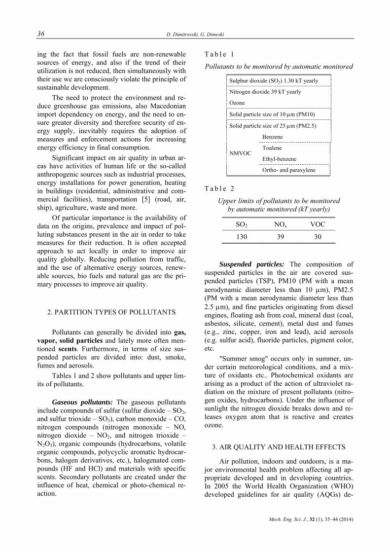
36 D. Dimitrovski, G. Dimeski
Mech. Eng. Sci. J., 32 (1), 35–44 (2014)
ing the fact that fossil fuels are non-renewable sources of energy, and also if the trend of their utilization is not reduced, then simultaneously with their use we are consciously violate the principle of sustainable development.
The need to protect the environment and re-duce greenhouse gas emissions, also Macedonian import dependency on energy, and the need to en-sure greater diversity and therefore security of en-ergy supply, inevitably requires the adoption of measures and enforcement actions for increasing energy efficiency in final consumption.
Significant impact on air quality in urban ar-eas have activities of human life or the so-called anthropogenic sources such as industrial processes, energy installations for power generation, heating in buildings (residential, administrative and com-mercial facilities), transportation [5] (road, air, ship), agriculture, waste and more.
Of particular importance is the availability of data on the origins, prevalence and impact of pol-luting substances present in the air in order to take measures for their reduction. It is often accepted approach to act locally in order to improve air quality globally. Reducing pollution from traffic, and the use of alternative energy sources, renew-able sources, bio fuels and natural gas are the pri-mary processes to improve air quality.
2. PARTITION TYPES OF POLLUTANTS
Pollutants can generally be divided into gas, vapor, solid particles and lately more often men-tioned scents. Furthermore, in terms of size sus-pended particles are divided into: dust, smoke, fumes and aerosols.
Tables 1 and 2 show pollutants and upper lim-its of pollutants.
Gaseous pollutants: The gaseous pollutants include compounds of sulfur (sulfur dioxide – SO2, and sulfur trioxide – SO3), carbon monoxide – CO, nitrogen compounds (nitrogen monoxide – NO, nitrogen dioxide – NO2, and nitrogen trioxide – N2O3), organic compounds (hydrocarbons, volatile organic compounds, polycyclic aromatic hydrocar-bons, halogen derivatives, etc.), halogenated com-pounds (HF and HCl) and materials with specific scents. Secondary pollutants are created under the influence of heat, chemical or photo-chemical re-action.
T a b l e 1
Pollutants to be monitored by automatic monitored
Sulphur dioxide (SO2) 1.30 kT yearly
Nitrogen dioxide 39 kT yearly
Ozone
Solid particle size of 10 µm (PM10)
Solid particle size of 25 µm (PM2.5)
Benzene
Toulene
Ethyl-benzene NMVOC
Ortho- and paraxylene
T a b l e 2
Upper limits of pollutants to be monitored by automatic monitored (kT yearly)
SO2 NOx VOC
130 39 30
Suspended particles: The composition of suspended particles in the air are covered sus-pended particles (TSP), PM10 (PM with a mean aerodynamic diameter less than 10 µm), PM2.5 (PM with a mean aerodynamic diameter less than 2.5 µm), and fine particles originating from diesel engines, floating ash from coal, mineral dust (coal, asbestos, silicate, cement), metal dust and fumes (e.g., zinc, copper, iron and lead), acid aerosols (e.g. sulfur acid), fluoride particles, pigment color, etc.
"Summer smog" occurs only in summer, un-der certain meteorological conditions, and a mix-ture of oxidants etc.. Photochemical oxidants are arising as a product of the action of ultraviolet ra-diation on the mixture of present pollutants (nitro-gen oxides, hydrocarbons). Under the influence of sunlight the nitrogen dioxide breaks down and re-leases oxygen atom that is reactive and creates ozone.
3. AIR QUALITY AND HEALTH EFFECTS
Air pollution, indoors and outdoors, is a ma-jor environmental health problem affecting all ap-propriate developed and in developing countries. In 2005 the World Health Organization (WHO) developed guidelines for air quality (AQGs) de-
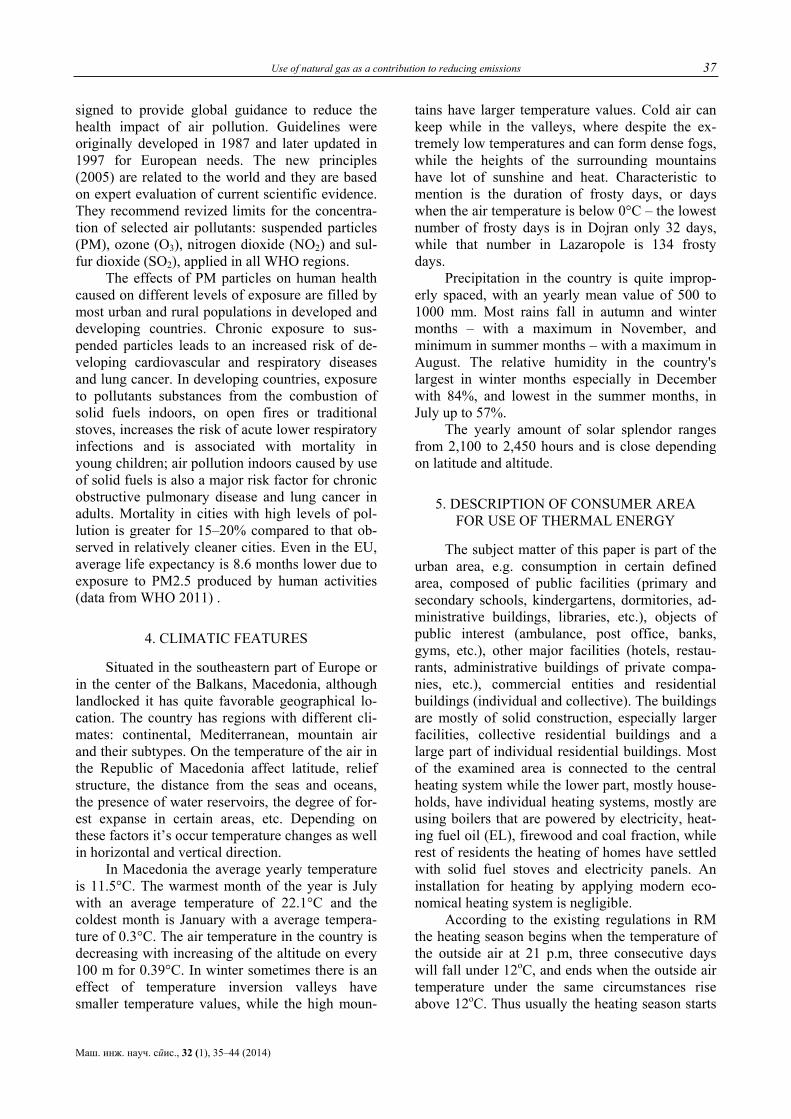
Use of natural gas as a contribution to reducing emissions 37
Маш. инж. науч. спис., 32 (1), 35–44 (2014)
signed to provide global guidance to reduce the health impact of air pollution. Guidelines were originally developed in 1987 and later updated in 1997 for European needs. The new principles (2005) are related to the world and they are based on expert evaluation of current scientific evidence. They recommend revized limits for the concentra-tion of selected air pollutants: suspended particles (PM), ozone (O3), nitrogen dioxide (NO2) and sul-fur dioxide (SO2), applied in all WHO regions.
The effects of PM particles on human health caused on different levels of exposure are filled by most urban and rural populations in developed and developing countries. Chronic exposure to sus-pended particles leads to an increased risk of de-veloping cardiovascular and respiratory diseases and lung cancer. In developing countries, exposure to pollutants substances from the combustion of solid fuels indoors, on open fires or traditional stoves, increases the risk of acute lower respiratory infections and is associated with mortality in young children; air pollution indoors caused by use of solid fuels is also a major risk factor for chronic obstructive pulmonary disease and lung cancer in adults. Mortality in cities with high levels of pol-lution is greater for 15–20% compared to that ob-served in relatively cleaner cities. Even in the EU, average life expectancy is 8.6 months lower due to exposure to PM2.5 produced by human activities (data from WHO 2011) .
4. CLIMATIC FEATURES
Situated in the southeastern part of Europe or in the center of the Balkans, Macedonia, although landlocked it has quite favorable geographical lo-cation. The country has regions with different cli-mates: continental, Mediterranean, mountain air and their subtypes. On the temperature of the air in the Republic of Macedonia affect latitude, relief structure, the distance from the seas and oceans, the presence of water reservoirs, the degree of for-est expanse in certain areas, etc. Depending on these factors it’s occur temperature changes as well in horizontal and vertical direction.
In Macedonia the average yearly temperature is 11.5°C. The warmest month of the year is July with an average temperature of 22.1°C and the coldest month is January with a average tempera-ture of 0.3°C. The air temperature in the country is decreasing with increasing of the altitude on every 100 m for 0.39°C. In winter sometimes there is an effect of temperature inversion valleys have smaller temperature values, while the high moun-
tains have larger temperature values. Cold air can keep while in the valleys, where despite the ex-tremely low temperatures and can form dense fogs, while the heights of the surrounding mountains have lot of sunshine and heat. Characteristic to mention is the duration of frosty days, or days when the air temperature is below 0°C – the lowest number of frosty days is in Dojran only 32 days, while that number in Lazaropole is 134 frosty days.
Precipitation in the country is quite improp-erly spaced, with an yearly mean value of 500 to 1000 mm. Most rains fall in autumn and winter months – with a maximum in November, and minimum in summer months – with a maximum in August. The relative humidity in the country's largest in winter months especially in December with 84%, and lowest in the summer months, in July up to 57%.
The yearly amount of solar splendor ranges from 2,100 to 2,450 hours and is close depending on latitude and altitude.
5. DESCRIPTION OF CONSUMER AREA FOR USE OF THERMAL ENERGY
The subject matter of this paper is part of the urban area, e.g. consumption in certain defined area, composed of public facilities (primary and secondary schools, kindergartens, dormitories, ad-ministrative buildings, libraries, etc.), objects of public interest (ambulance, post office, banks, gyms, etc.), other major facilities (hotels, restau-rants, administrative buildings of private compa-nies, etc.), commercial entities and residential buildings (individual and collective). The buildings are mostly of solid construction, especially larger facilities, collective residential buildings and a large part of individual residential buildings. Most of the examined area is connected to the central heating system while the lower part, mostly house-holds, have individual heating systems, mostly are using boilers that are powered by electricity, heat-ing fuel oil (EL), firewood and coal fraction, while rest of residents the heating of homes have settled with solid fuel stoves and electricity panels. An installation for heating by applying modern eco-nomical heating system is negligible.
According to the existing regulations in RM the heating season begins when the temperature of the outside air at 21 p.m, three consecutive days will fall under 12oС, and ends when the outside air temperature under the same circumstances rise above 12oС. Thus usually the heating season starts
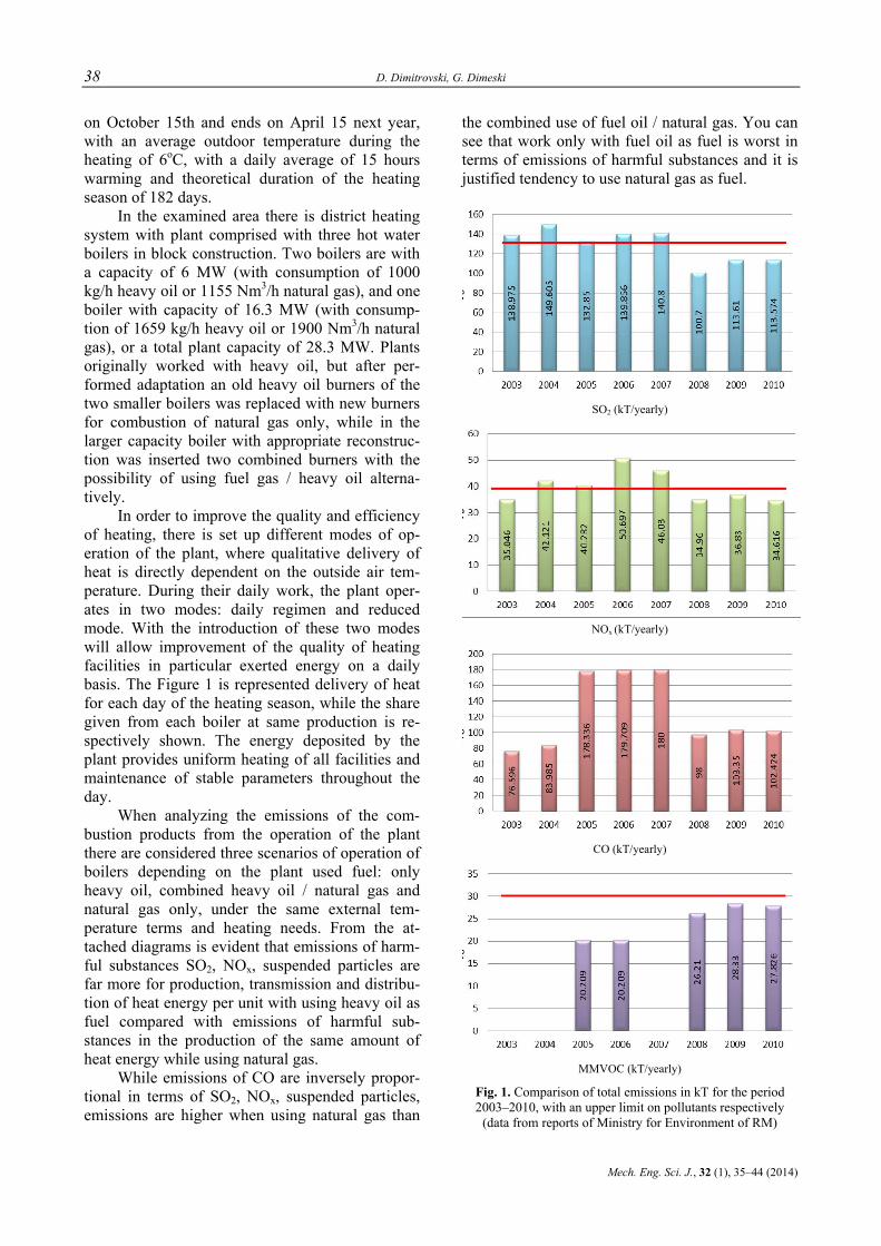
38 D. Dimitrovski, G. Dimeski
Mech. Eng. Sci. J., 32 (1), 35–44 (2014)
on October 15th and ends on April 15 next year, with an average outdoor temperature during the heating of 6oС, with a daily average of 15 hours warming and theoretical duration of the heating season of 182 days.
In the examined area there is district heating system with plant comprised with three hot water boilers in block construction. Two boilers are with a capacity of 6 MW (with consumption of 1000 kg/h heavy oil or 1155 Nm3/h natural gas), and one boiler with capacity of 16.3 MW (with consump-tion of 1659 kg/h heavy oil or 1900 Nm3/h natural gas), or a total plant capacity of 28.3 MW. Plants originally worked with heavy oil, but after per-formed adaptation an old heavy oil burners of the two smaller boilers was replaced with new burners for combustion of natural gas only, while in the larger capacity boiler with appropriate reconstruc-tion was inserted two combined burners with the possibility of using fuel gas / heavy oil alterna-tively.
In order to improve the quality and efficiency of heating, there is set up different modes of op-eration of the plant, where qualitative delivery of heat is directly dependent on the outside air tem-perature. During their daily work, the plant oper-ates in two modes: daily regimen and reduced mode. With the introduction of these two modes will allow improvement of the quality of heating facilities in particular exerted energy on a daily basis. The Figure 1 is represented delivery of heat for each day of the heating season, while the share given from each boiler at same production is re-spectively shown. The energy deposited by the plant provides uniform heating of all facilities and maintenance of stable parameters throughout the day.
When analyzing the emissions of the com-bustion products from the operation of the plant there are considered three scenarios of operation of boilers depending on the plant used fuel: only heavy oil, combined heavy oil / natural gas and natural gas only, under the same external tem-perature terms and heating needs. From the at-tached diagrams is evident that emissions of harm-ful substances SO2, NOx, suspended particles are far more for production, transmission and distribu-tion of heat energy per unit with using heavy oil as fuel compared with emissions of harmful sub-stances in the production of the same amount of heat energy while using natural gas.
While emissions of CO are inversely propor-tional in terms of SO2, NOx, suspended particles, emissions are higher when using natural gas than
the combined use of fuel oil / natural gas. You can see that work only with fuel oil as fuel is worst in terms of emissions of harmful substances and it is justified tendency to use natural gas as fuel.
SO2 (kT/yearly)
NOx (kT/yearly)
CO (kT/yearly)
MMVOC (kT/yearly)
Fig. 1. Comparison of total emissions in kT for the period 2003–2010, with an upper limit on pollutants respectively
(data from reports of Ministry for Environment of RM)
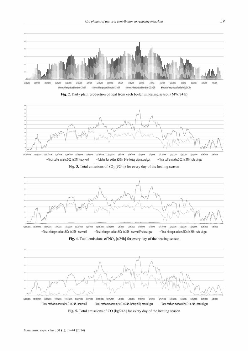
Use of natural gas as a contribution to reducing emissions 39
Маш. инж. науч. спис., 32 (1), 35–44 (2014)
0
100
200
300
400
500
600
10/10/2005 10/20/2005 10/30/2005 11/9/2005 11/19/2005 11/29/2005 12/9/2005 12/19/2005 12/29/2005 1/8/2006 1/18/2006 1/28/2006 2/7/2006 2/17/2006 2/27/2006 3/9/2006 3/19/2006 3/29/2006 4/8/2006
Amount of heat produced from boiler K1 in 24h Amount of heat produced from boiler K2 in 24h Amount of heat produced from boiler K3/1 in 24h Amount of heat produced from boiler K3/2 in 24h Fig. 2. Daily plant production of heat from each boiler in heating season (MW/24 h)
0
200
400
600
800
1000
1200
1400
1600
1800
2000
2200
2400
10/10/2005 10/20/2005 10/30/2005 11/9/2005 11/19/2005 11/29/2005 12/9/2005 12/19/2005 12/29/2005 1/8/2006 1/18/2006 1/28/2006 2/7/2006 2/17/2006 2/27/2006 3/9/2006 3/19/2006 3/29/2006 4/8/2006
Total sulfur oxides SO2 in 24h ‐heavy oil Total sulfur oxides SO2 in 24h‐ heavy oil/natural gas Total sulfur oxides SO2 in 24h‐ natural gas Fig. 3. Total emissions of SO2 (t/24h) for every day of the heating season
0
50
100
150
200
250
300
350
400
0/10/2005 10/20/2005 10/30/2005 11/9/2005 11/19/2005 11/29/2005 12/9/2005 12/19/2005 12/29/2005 1/8/2006 1/18/2006 1/28/2006 2/7/2006 2/17/2006 2/27/2006 3/9/2006 3/19/2006 3/29/2006 4/8/2006
Total nitrogen oxides NOx in 24h‐ heavy oil Total nitrogen oxides NOx in 24h‐ heavy oil/natural gas Total nitrogen oxides NOx in 24h‐ natural gas Fig. 4. Total emissions of NOx [t/24h] for every day of the heating season
0
100
200
300
400
500
600
0/10/2005 10/20/2005 10/30/2005 11/9/2005 11/19/2005 11/29/2005 12/9/2005 12/19/2005 12/29/2005 1/8/2006 1/18/2006 1/28/2006 2/7/2006 2/17/2006 2/27/2006 3/9/2006 3/19/2006 3/29/2006 4/8/2006
Total carbon monoxide CO in 24h‐ heavy oil Total carbon monoxide CO in 24h‐ heavy oil / natural gas Total carbon monoxide CO in 24h‐ natural gas Fig. 5. Total emissions of CO [kg/24h] for every day of the heating season
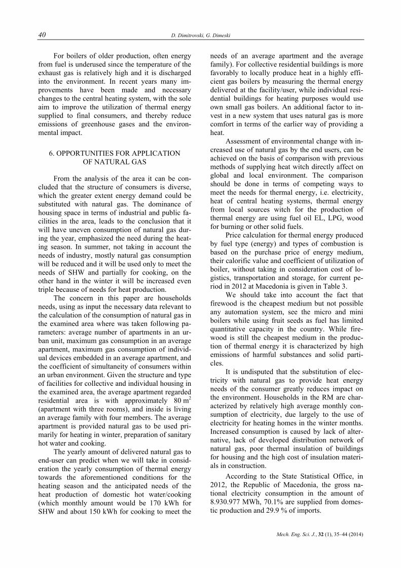
40 D. Dimitrovski, G. Dimeski
Mech. Eng. Sci. J., 32 (1), 35–44 (2014)
For boilers of older production, often energy from fuel is underused since the temperature of the exhaust gas is relatively high and it is discharged into the environment. In recent years many im-provements have been made and necessary changes to the central heating system, with the sole aim to improve the utilization of thermal energy supplied to final consumers, and thereby reduce emissions of greenhouse gases and the environ-mental impact.
6. OPPORTUNITIES FOR APPLICATION OF NATURAL GAS
From the analysis of the area it can be con-cluded that the structure of consumers is diverse, which the greater extent energy demand could be substituted with natural gas. The dominance of housing space in terms of industrial and public fa-cilities in the area, leads to the conclusion that it will have uneven consumption of natural gas dur-ing the year, emphasized the need during the heat-ing season. In summer, not taking in account the needs of industry, mostly natural gas consumption will be reduced and it will be used only to meet the needs of SHW and partially for cooking, on the other hand in the winter it will be increased even triple because of needs for heat production.
The concern in this paper are households needs, using as input the necessary data relevant to the calculation of the consumption of natural gas in the examined area where was taken following pa-rameters: average number of apartments in an ur-ban unit, maximum gas consumption in an average apartment, maximum gas consumption of individ-ual devices embedded in an average apartment, and the coefficient of simultaneity of consumers within an urban environment. Given the structure and type of facilities for collective and individual housing in the examined area, the average apartment regarded residential area is with approximately 80 m2 (apartment with three rooms), and inside is living an average family with four members. The average apartment is provided natural gas to be used pri-marily for heating in winter, preparation of sanitary hot water and cooking.
The yearly amount of delivered natural gas to end-user can predict when we will take in consid-eration the yearly consumption of thermal energy towards the aforementioned conditions for the heating season and the anticipated needs of the heat production of domestic hot water/cooking (which monthly amount would be 170 kWh for SHW and about 150 kWh for cooking to meet the
needs of an average apartment and the average family). For collective residential buildings is more favorably to locally produce heat in a highly effi-cient gas boilers by measuring the thermal energy delivered at the facility/user, while individual resi-dential buildings for heating purposes would use own small gas boilers. An additional factor to in-vest in a new system that uses natural gas is more comfort in terms of the earlier way of providing a heat.
Assessment of environmental change with in-creased use of natural gas by the end users, can be achieved on the basis of comparison with previous methods of supplying heat witch directly affect on global and local environment. The comparison should be done in terms of competing ways to meet the needs for thermal energy, i.e. electricity, heat of central heating systems, thermal energy from local sources witch for the production of thermal energy are using fuel oil EL, LPG, wood for burning or other solid fuels.
Price calculation for thermal energy produced by fuel type (energy) and types of combustion is based on the purchase price of energy medium, their calorific value and coefficient of utilization of boiler, without taking in consideration cost of lo-gistics, transportation and storage, for current pe-riod in 2012 at Macedonia is given in Table 3.
We should take into account the fact that firewood is the cheapest medium but not possible any automation system, see the micro and mini boilers while using fruit seeds as fuel has limited quantitative capacity in the country. While fire-wood is still the cheapest medium in the produc-tion of thermal energy it is characterized by high emissions of harmful substances and solid parti-cles.
It is undisputed that the substitution of elec-tricity with natural gas to provide heat energy needs of the consumer greatly reduces impact on the environment. Households in the RM are char-acterized by relatively high average monthly con-sumption of electricity, due largely to the use of electricity for heating homes in the winter months. Increased consumption is caused by lack of alter-native, lack of developed distribution network of natural gas, poor thermal insulation of buildings for housing and the high cost of insulation materi-als in construction.
According to the State Statistical Office, in 2012, the Republic of Macedonia, the gross na-tional electricity consumption in the amount of 8.930.977 MWh, 70.1% are supplied from domes-tic production and 29.9 % of imports.
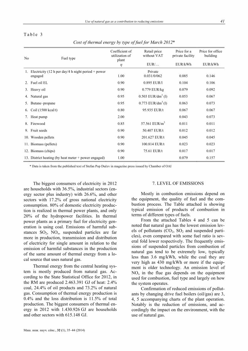
Use of natural gas as a contribution to reducing emissions 41
Маш. инж. науч. спис., 32 (1), 35–44 (2014)
T a b l e 3
Cost of thermal energy by type of fuel for March 2012*
Coefficient of utilization of
plant
Retail price without VAT
Price for a private facility
Price for office building
No Fuel type
η EUR/… EUR/kWh EUR/kWh
1. Electricity (12 h per day/4 h night period + power engaged 1.00
Private 0.031/0/062 0.085 0.146
2. Fuel oil EL 0.90 0.895 EUR/l 0.104 0.106
3. Heavy oil 0.90 0.779 EUR/kg 0.079 0.092
4. Natural gas 0.95 0.503 EUR/dm3 (l) 0.053 0.067
5. Butane–propane 0.95 0.773 EUR/dm3 (l) 0.063 0.073
6. Coil (1500 kcal/t) 0.80 95.935 EUR/t 0.067 0.067
7. Heat pump 2.00 0.043 0.073
8. Firewood 0.85 57.561 EUR/m3 0.011 0.011
9. Fruit seeds 0.90 50.407 EUR/t 0.012 0.012
10. Wooden pellets 0.90 201.627 EUR/t 0.045 0.045
11. Biomass (pellets) 0.90 100.814 EUR/t 0.023 0.023
12. Biomass (chips) 0.90 75.61 EUR/t 0.017 0.017
13. District heating (by heat meter + power engaged) 1.00 0.079 0.157
* Data is taken from the published text of Stefan Pop Dučev in magazine press issued by Chamber of OAI
The biggest consumers of electricity in 2012 are households with 36.5%, industrial sectors (en-ergy sector plus industry) with 26.6%, and other sectors with 17.2% of gross national electricity consumption. 80% of domestic electricity produc-tion is realized in thermal power plants, and only 20% of the hydropower facilities. In thermal power plants as a primary fuel for electricity gen-eration is using coal. Emissions of harmful sub-stances SO2, NOx, suspended particles are far more in production, transmission and distribution of electricity for single amount in relation to the emission of harmful substances in the production of the same amount of thermal energy from a lo-cal source that uses natural gas.
Thermal energy from the central heating sys-tem is mostly produced from natural gas. Ac-cording to the State Statistical Office for 2012, in the RM are produced 2.463.391 GJ of heat: 2.4% coal, 24.4% of oil products and 73.2% of natural gas. Consumption of thermal energy production is 0.4% and the loss distribution is 11.5% of total production. The biggest consumers of thermal en-ergy in 2012 with 1.430.926 GJ are households and other sectors with 615.148 GJ.
7. LEVEL OF EMISSIONS
Mostly in combustion emissions depend on the equipment, the quality of fuel and the com-bustion process. The Table attached is showing typical emission of products of combustion in terms of different types of fuels.
From the attached Tables 4 and 5 can be noted that natural gas has the lowest emission lev-els of pollutants (CO2, SO2 and suspended parti-cles), even compared with some fuel ratio is sev-eral fold lower respectively. The frequently emis-sions of suspended particles from combustion of natural gas tend to be extremely low, typically less than 3.6 mg/kWh, while the coal they are very high as 430 mg/kWh or more if the equip-ment is older technology. An emission level of NOx in the flue gas depends on the equipment used for combustion, fuel type and largely on how the system operates.
Confirmation of reduced emissions of pollut-ants by changing drive fuel boilers (oil/gas) are 3, 4, 5 accompanying charts of the plant operation. Notably is the reduction of emissions, and ac-cordingly the impact on the environment, with the use of natural gas.
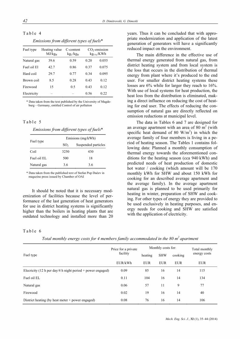
42 D. Dimitrovski, G. Dimeski
Mech. Eng. Sci. J., 32 (1), 35–44 (2014)
T a b l e 4
Emissions from different types of fuels*
Fuel type Heating value C-content CO2-emission MJ/kgB kgC/kgB kgCO2/KWh
Natural gas 39.6 0.59 0.20 0.055
Fuel oil El 42.7 0.86 0.37 0.075
Hard coil 29.7 0.77 0.34 0.095
Brown coil 8.5 0.28 0.43 0.12
Firewood 15 0.5 0.43 0.12
Electricity – – 0.56 0.22
* Data taken from the text published by the University of Magde-burg – Germany, entitled Control of air pollution
T a b l e 5
Emissions from different types of fuels*
Emisions (mg/kWh) Fuel type
SO2 Suspended particles
Coil 3250 430
Fuel oil EL 500 18
Natural gas 3.6 3.6
* Data taken from the published text of Stefan Pop Dučev in magazine press issued by Chamber of OAI
It should be noted that it is necessary mod-ernization of facilities because the level of per-formance of the last generation of heat generators for use in district heating systems is significantly higher than the boilers in heating plants that are outdated technology and installed more than 20
years. Thus it can be concluded that with appro-priate modernization and application of the latest generation of generators will have a significantly reduced impact on the environment.
The main difference in the effective use of thermal energy generated from natural gas, from district heating system and from local system is the loss that occurs in the distribution of thermal energy from plant where it’s produced to the end user. For smaller district heating systems these losses are 6% while for larger they reach to 16%. With use of local systems for heat production, the heat loss from the distribution is eliminated, mak-ing a direct influence on reducing the cost of heat-ing for end user. The effects of reducing the con-sumption of natural gas are directly reflected on emission reductions at municipal level.
The data in Tables 6 and 7 are designed for an average apartment with an area of 80 m2 (with specific heat demand of 80 W/m2) in which the average family of four members is living in a pe-riod of heating season. The Tables 1 contains fol-lowing data: Planned a monthly consumption of thermal energy towards the aforementioned con-ditions for the heating season (cca 940 kWh) and predicted needs of heat production of domestic hot water / cooking (which amount will be 170 monthly kWh for SHW and about 150 kWh for cooking for an described average apartment and the average family). In the average apartment natural gas is planned to be used primarily for heating in winter, preparation of SHW and cook-ing. For other types of energy they are provided to be used exclusively in heating purposes, and en-ergy needs for cooking and SHW are satisfied with the application of electricity.
T a b l e 6
Total monthly energy costs for 4 members family accommodated in the 80 m2 apartment
Monthly costs for: Price for a private facility heating SHW cooking
Total monthly energy costs Fuel type
EUR/kWh EUR EUR EUR EUR
Elecricity (12 h per day/4 h night period + power engaged) 0.09 85 16 14 115
Fuel oil EL 0.11 104 16 14 134
Natural gas 0.06 57 11 9 77
Firewood 0.02 19 16 14 40
District heating (by heat meter + power engaged) 0.08 76 16 14 106
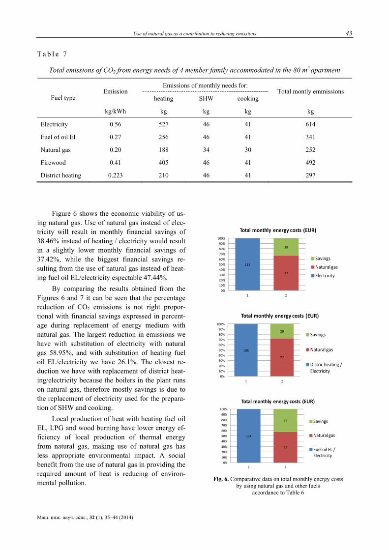
Use of natural gas as a contribution to reducing emissions 43
Маш. инж. науч. спис., 32 (1), 35–44 (2014)
T a b l e 7
Total emissions of CO2 from energy needs of 4 member family accommodated in the 80 m2 apartment
Emissions of monthly needs for: Emission
heating SHW cooking Total montly emmissions
Fuel type
kg/kWh kg kg kg kg
Electricity 0.56 527 46 41 614
Fuel of oil El 0.27 256 46 41 341
Natural gas 0.20 188 34 30 252
Firewood 0.41 405 46 41 492
District heating 0.223 210 46 41 297
Figure 6 shows the economic viability of us-
ing natural gas. Use of natural gas instead of elec-tricity will result in monthly financial savings of 38.46% instead of heating / electricity would result in a slightly lower monthly financial savings of 37.42%, while the biggest financial savings re-sulting from the use of natural gas instead of heat-ing fuel oil EL/electricity espectable 47.44%.
By comparing the results obtained from the Figures 6 and 7 it can be seen that the percentage reduction of CO2 emissions is not right propor-tional with financial savings expressed in percent-age during replacement of energy medium with natural gas. The largest reduction in emissions we have with substitution of electricity with natural gas 58.95%, and with substitution of heating fuel oil EL/electricity we have 26.1%. The closest re-duction we have with replacement of district heat-ing/electricity because the boilers in the plant runs on natural gas, therefore mostly savings is due to the replacement of electricity used for the prepara-tion of SHW and cooking.
Local production of heat with heating fuel oil EL, LPG and wood burning have lower energy ef-ficiency of local production of thermal energy from natural gas, making use of natural gas has less appropriate environmental impact. A social benefit from the use of natural gas in providing the required amount of heat is reducing of environ-mental pollution.
115
77
38
0%10%20%30%40%50%60%70%80%90%100%
1 2
Total monthly energy costs (EUR)
Savings
Natural gas
Electricity
106
77
29
0%
10%20%
30%40%50%
60%70%
80%90%
100%
1 2
Total monthly energy costs (EUR)
Savings
Natural gas
Distric heating / Electricity
134
77
57
0%
10%
20%
30%
40%
50%
60%
70%
80%
90%
100%
1 2
Total monthly energy costs (EUR)
Savings
Natural gas
Fuel oil EL / Electricity
Fig. 6. Comparative data on total monthly energy costs
by using natural gas and other fuels accordance to Table 6
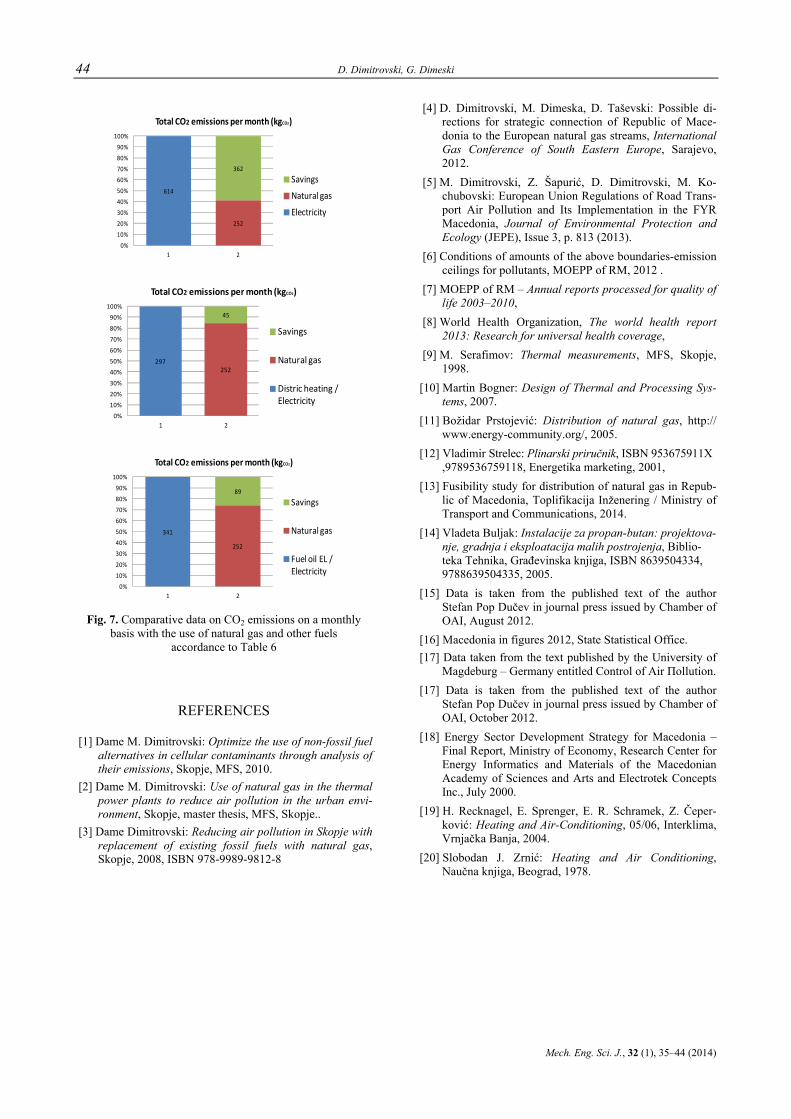
44 D. Dimitrovski, G. Dimeski
Mech. Eng. Sci. J., 32 (1), 35–44 (2014)
614
252
362
0%
10%
20%
30%
40%
50%
60%
70%
80%
90%
100%
1 2
Total CO2 emissions per month (kgCO2)
Savings
Natural gas
Electricity
297252
45
0%
10%
20%
30%
40%
50%
60%
70%
80%
90%
100%
1 2
Total CO2 emissions per month (kgCO2)
Savings
Natural gas
Distric heating / Electricity
341
252
89
0%
10%
20%
30%
40%
50%
60%
70%
80%
90%
100%
1 2
Total CO2 emissions per month (kgCO2)
Savings
Natural gas
Fuel oil EL / Electricity
Fig. 7. Comparative data on CO2 emissions on a monthly
basis with the use of natural gas and other fuels accordance to Table 6
REFERENCES
[1] Dame M. Dimitrovski: Optimize the use of non-fossil fuel alternatives in cellular contaminants through analysis of their emissions, Skopje, MFS, 2010.
[2] Dame M. Dimitrovski: Use of natural gas in the thermal power plants to reduce air pollution in the urban envi-ronment, Skopje, master thesis, MFS, Skopje..
[3] Dame Dimitrovski: Reducing air pollution in Skopje with replacement of existing fossil fuels with natural gas, Skopje, 2008, ISBN 978-9989-9812-8
[4] D. Dimitrovski, M. Dimeska, D. Taševski: Possible di-rections for strategic connection of Republic of Mace-donia to the European natural gas streams, International Gas Conference of South Eastern Europe, Sarajevo, 2012.
[5] M. Dimitrovski, Z. Šapurić, D. Dimitrovski, M. Ko-chubovski: European Union Regulations of Road Trans-port Air Pollution and Its Implementation in the FYR Macedonia, Journal of Environmental Protection and Ecology (JEPE), Issue 3, p. 813 (2013).
[6] Conditions of amounts of the above boundaries-emission ceilings for pollutants, MOEPP of RM, 2012 .
[7] MOEPP of RM – Annual reports processed for quality of life 2003–2010,
[8] World Health Organization, The world health report 2013: Research for universal health coverage,
[9] М. Serafimov: Thermal measurements, MFS, Skopje, 1998.
[10] Martin Bogner: Design of Thermal and Processing Sys-tems, 2007.
[11] Božidar Prstojević: Distribution of natural gas, http:// www.energy-community.org/, 2005.
[12] Vladimir Strelec: Plinarski priručnik, ISBN 953675911X ,9789536759118, Energetika marketing, 2001,
[13] Fusibility study for distribution of natural gas in Repub-lic of Macedonia, Toplifikacija Inženering / Ministry of Transport and Communications, 2014.
[14] Vladeta Buljak: Instalacije za propan-butan: projektova-nje, gradnja i eksploatacija malih postrojenja, Biblio-teka Tehnika, Građevinska knjiga, ISBN 8639504334, 9788639504335, 2005.
[15] Data is taken from the published text of the author Stefan Pop Dučev in journal press issued by Chamber of OAI, August 2012.
[16] Macedonia in figures 2012, State Statistical Office. [17] Data taken from the text published by the University of
Magdeburg – Germany entitled Control of Аir Пollution. [17] Data is taken from the published text of the author
Stefan Pop Dučev in journal press issued by Chamber of OAI, October 2012.
[18] Energy Sector Development Strategy for Macedonia – Final Report, Ministry of Economy, Research Center for Energy Informatics and Materials of the Macedonian Academy of Sciences and Arts and Electrotek Concepts Inc., July 2000.
[19] H. Recknagel, E. Sprenger, E. R. Schramek, Z. Čeper-ković: Heating and Air-Conditioning, 05/06, Interklima, Vrnjačka Banja, 2004.
[20] Slobodan J. Zrnić: Heating and Air Conditioning, Naučna knjiga, Beograd, 1978.

Mechanical Engineering – Scientific Journal, Vol. 32, No. 1, pp. 45–49 (2014) CODEN: MINSC5 – 452 In print: ISSN 1857–5293 Received: March 1, 2014 On line: ISSN 1857–9191 Accepted: April 20, 2014 UDC: 69.05:620.92
Original scientific paper
SUSTAINABLE IMPROVEMENT OF THE ENERGY EFFICIENCY OF AN EXISTING BUILDING
Aleksandar Petrovski1, Atanas Kočov2, Valentina Zileska Pančovska3 1"Ss Cyril and Methodius" University in Skopje, Faculty of Architecture,
Blvd. Partizanski odredi 24, Skopje, Republic of Macedonia 2"Ss. Cyril and Methodius" University in Skopje, Faculty of Mechanical Engineering,
Karpoš II bb, P.O. box 464, 1001 Skopje, Republic of Macedonia 3"Ss Cyril and Methodius" University in Skopje, Faculty of Civil Engineering,
Blvd. Partizanski odredi 24, Skopje, Republic of Macedonia [email protected]
A b s t r a c t: The existing housing buildings are consumers of large quantities of energy due to the low ther-mal characteristics of the buildings envelope. The ground-floor housing buildings represent large percentage of the housing stock in Republic of Macedonia. Тhree possibilities for achieving environmental sustainability of a building are analyzed such as: improvement of the energy efficiency of the buildings walls, the windows and both options al-together. The possibilities consider the improvement of the energy performance of the facade related with financial issues such as bank credit and investment return. Autodesk Ecotect is used for the modelling and energy performance simulation. From the results it is concluded that the investment return period is very long and certain measures need to be taken such as decreasing the loans interest rate, decreasing the building cost and materials and providing possi-bilities for subsidy.
Key words: sustainability; building envelope; bank credit; return of investment
ОДРЖЛИВО ПОДОБРУВАЊЕ НА ЕНЕРГЕТСКАТА ЕФИКАСНОСТ НА ПОСТОЕН ОБЈЕКТ
А п с т р а к т: Постојните станбени објекти се потрошувачи на големи количества енергија поради слабите термички карактеристики на фасадата и покривот. Приземните станбени објекти се застапени во голем процент во целокупниот станбен фонд во Република Македонија. За постоен приземен објект се разгледувани три можности со цел постигнување одржливост на објектот во однос на околината, и тоа преку подобрување на енергетските карактеристики на надворешните ѕидови, на прозорците и двете опции заедно. Можностите се однесуваат на подобрување на енергетските перформанси на објектот поставени во релација со финансиските аспекти како што се банкарски кредити и враќање на инвестицијата. За моделирањето на енергетските перформанси на објектот е употребен софтверот Autodesk Ecotect. Од добиените резултати е заклучено дека рокот на враќањето на инвестиција е долг, поради што е потребно да се преземат чекори во однос на намалување на каматните стапки за кредити, намалување на градежните трошоци и создавање можности за субвенционирање.
Клучни зборови: одржливост; надворешни ѕидови на објект; кредити; враќање на инвестиција
1. INTRODUCTION
Modern society is confronted with transfor-mation imposed by the climatic changes. The con-struction sector reached a consensus about the in-
fluence of the built environment in causing these climatic changes [1]. According to the studies of the yearly emission of CO2 per capita, 30% from all the emissions are from the heating of buildings, 28% from the cars, etc. [5].
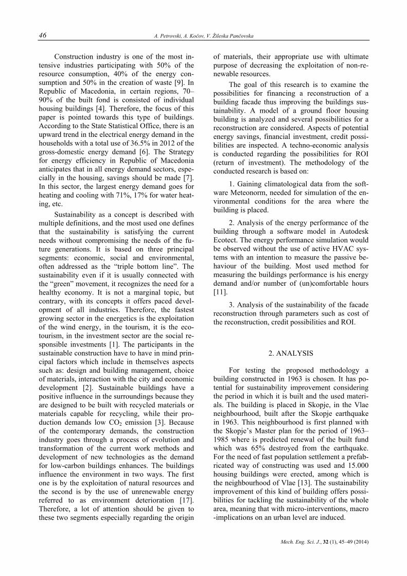
46 A. Petrovski, A. Kočov, V. Žileska Pančovska
Mech. Eng. Sci. J., 32 (1), 45–49 (2014)
Construction industry is one of the most in-tensive industries participating with 50% of the resource consumption, 40% of the energy con-sumption and 50% in the creation of waste [9]. In Republic of Macedonia, in certain regions, 70–90% of the built fond is consisted of individual housing buildings [4]. Therefore, the focus of this paper is pointed towards this type of buildings. According to the State Statistical Office, there is an upward trend in the electrical energy demand in the households with a total use of 36.5% in 2012 of the gross-domestic energy demand [6]. The Strategy for energy efficiency in Republic of Macedonia anticipates that in all energy demand sectors, espe-cially in the housing, savings should be made [7]. In this sector, the largest energy demand goes for heating and cooling with 71%, 17% for water heat-ing, etc.
Sustainability as a concept is described with multiple definitions, and the most used one defines that the sustainability is satisfying the current needs without compromising the needs of the fu-ture generations. It is based on three principal segments: economic, social and environmental, often addressed as the “triple bottom line”. The sustainability even if it is usually connected with the “green” movement, it recognizes the need for a healthy economy. It is not a marginal topic, but contrary, with its concepts it offers paced devel-opment of all industries. Therefore, the fastest growing sector in the energetics is the exploitation of the wind energy, in the tourism, it is the eco-tourism, in the investment sector are the social re-sponsible investments [1]. The participants in the sustainable construction have to have in mind prin-cipal factors which include in themselves aspects such as: design and building management, choice of materials, interaction with the city and economic development [2]. Sustainable buildings have a positive influence in the surroundings because they are designed to be built with recycled materials or materials capable for recycling, while their pro-duction demands low CO2 emission [3]. Because of the contemporary demands, the construction industry goes through a process of evolution and transformation of the current work methods and development of new technologies as the demand for low-carbon buildings enhances. The buildings influence the environment in two ways. The first one is by the exploitation of natural resources and the second is by the use of unrenewable energy referred to as environment deterioration [17]. Therefore, a lot of attention should be given to these two segments especially regarding the origin
of materials, their appropriate use with ultimate purpose of decreasing the exploitation of non-re-newable resources.
The goal of this research is to examine the possibilities for financing a reconstruction of a building facade thus improving the buildings sus-tainability. A model of a ground floor housing building is analyzed and several possibilities for a reconstruction are considered. Aspects of potential energy savings, financial investment, credit possi-bilities are inspected. A techno-economic analysis is conducted regarding the possibilities for ROI (return of investment). The methodology of the conducted research is based on:
1. Gaining climatological data from the soft-ware Meteonorm, needed for simulation of the en-vironmental conditions for the area where the building is placed.
2. Analysis of the energy performance of the building through a software model in Autodesk Ecotect. The energy performance simulation would be observed without the use of active HVAC sys-tems with an intention to measure the passive be-haviour of the building. Most used method for measuring the buildings performance is his energy demand and/or number of (un)comfortable hours [11].
3. Analysis of the sustainability of the facade reconstruction through parameters such as cost of the reconstruction, credit possibilities and ROI.
2. ANALYSIS
For testing the proposed methodology a building constructed in 1963 is chosen. It has po-tential for sustainability improvement considering the period in which it is built and the used materi-als. The building is placed in Skopje, in the Vlae neighbourhood, built after the Skopje earthquake in 1963. This neighbourhood is first planned with the Skopje’s Master plan for the period of 1963–1985 where is predicted renewal of the built fund which was 65% destroyed from the earthquake. For the need of fast population settlement a prefab-ricated way of constructing was used and 15.000 housing buildings were erected, among which is the neighbourhood of Vlae [13]. The sustainability improvement of this kind of building offers possi-bilities for tackling the sustainability of the whole area, meaning that with micro-interventions, macro -implications on an urban level are induced.
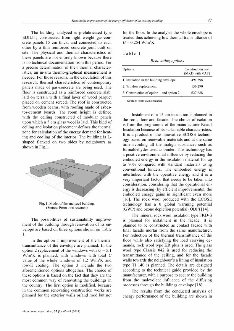
Sustainable improvement of the energy efficiency of an existing building 47
Маш. инж. науч. спис., 32 (1), 45–49 (2014)
The building analyzed is prefabricated type EDILIT, constructed from light weight gas-con-crete panels 15 cm thick, and connected to each other by a thin reinforced concrete joint built on site. The physical and thermal characteristics of these panels are not entirely known because there is no technical documentation from this period. For a precise determination of their thermal character-istics, an in-situ thermo-graphical measurement is needed. For those reasons, in the calculation of this research, thermal characteristics of contemporary panels made of gas-concrete are being used. The floor is constructed as a reinforced concrete slab, laid on terrain with a final layer of wood parquet placed on cement screed. The roof is constructed from wooden beams, with roofing made of asbes-tos-cement boards. The room height is defined with the ceiling constructed of modular panels upon which a 5 cm glass wool is laid. This kind of ceiling and isolation placement defines the thermal zone for calculation of the energy demand for heat-ing and cooling of the interior. The building is L-shaped flanked on two sides by neighbours as shown in Fig.1.
Fig. 1. Model of the analyzed building.
(Source: From own research)
The possibilities of sustainability improve-ment of the building through renovation of its en-velope are based on three options shown on Table 1.
In the option 1 improvement of the thermal transmittance of the envelope are planned. In the option 2 replacement of the windows with U = 5.1 W/m2K is planned, with windows with total U value of the whole windows of 1.2 W/m2K and low-E coating. The option 3 include the two aforementioned options altogether. The choice of these options is based on the fact that they are the most common way of renovating the buildings in the country. The first option is modified, because in the common renovating construction works are planned for the exterior walls or/and rood but not
for the floor. In the analysis the whole envelope is treated thus achieving low thermal transmittance of U = 0.254 W/m2K.
T a b l e 1
Renovating options
Options Construction cost (MKD with VAT)
1. Insulation in the building envelope 491.398
2. Window replacement 136.290
3. Construction of option 1 and option 2 627.688
Source: From own research
Instalment of a 15 cm insulation is planned in the roof, floor and facade. The choice of isolation is from the programme of the manufacturer Knauf Insulation because of its sustainable characteristics. It is a product of the innovative ECOSE technol-ogy based on renewable materials and at the same time avoiding all the malign substances such as formaldehydes used as binder. This technology has a positive environmental influence by reducing the embodied energy in the insulation material for up to 70% compared with standard materials using conventional binders. The embodied energy is interlinked with the operative energy and it is a very important factor that needs to be taken into consideration, considering that the operational en-ergy is decreasing (by efficient improvements), the embodied energy gains in significant even more [16]. The rock wool produced with the ECOSE technology has a 0 global warming potential (GWP) and ozone depletion potential (ODP) [14].
The mineral rock wool insulation type FKD-S is planned for instalment in the facade. It is planned to be constructed as contact facade with final facade mortar from the same manufacturer. For reduction of the thermal transmittance of the floor while also satisfying the load carrying de-mands, rock wool type KR plus is used. The glass wool type Classic 042 is used for reducing the transmittance of the ceiling, and for the facade walls towards the neighbour’s a lining of insulation type TI 140 is planned. The details are designed according to the technical guide provided by the manufacturer, with a purpose to secure the building from the malevolent influence of the diffusing processes through the buildings envelope [18].
The results from the conducted analysis of energy performance of the building are shown in

48 A. Petrovski, A. Kočov, V. Žileska Pančovska
Mech. Eng. Sci. J., 32 (1), 45–49 (2014)
Figure 2 from which it can be concluded that the decrease of energy losses in the reconstruction in option 1 is larger that in option 2. The existing windows have much larger coefficient of thermal transmittance, meaning that through them it occurs a large heat flow, and an expected result of the renovation would be to have largest saving with their replacement.
Fig. 2. Model of the analyzed building
(Source: From own research)
But, because of the large participation of the wall area in the total area of the envelope with 95.8%, while the windows participate with 4.2%, the largest heat losses are through the opaque sur-faces. The total yearly consumption of heating and cooling energy is shown in Table 2.
T a b l e 2
Energy and financial savings
Energy consump
Total yearly cost
Yearly savings
Monthly savings
kWh.a MKD MKD MKD
A0 – existing build. 5617 44.907 0 0
A1 – option 1 3136 25.072 19.835 1653
A2 – option 2 4043 32.323 12.584 1048
A3 – option 3 1562 12.488 32.419 2101
Source: From own research.
In Table 2 are shown the total energy con-sumption, yearly cost, yearly and monthly savings, from which it can be concluded that the largest energy savings are in the Option 3. The total en-ergy costs are calculated according to the current energy price of 0.13 €/kWh (7.9 MKD/kWh), with an expected tendency for its increase. In the next step of this research an analysis is conducted on
the possibilities of bank credits and ROI according to the monthly annuity and the monthly energy savings.
3. INVESTMENT SUSTAINABILITY
In Republic of Macedonia the banks offer dif-ferent credit options for realizing such a renova-tion. The loans can be met under the names as “green” credit or consumer credits. For fulfilling the right of taking credit, the borrower should meet certain demands such as: being employed (in the private or public sector, from which the interest rate depends), salary from which the payment pe-riod depends, possibilities for a co-signer, etc. De-pending of the bank, the monthly annuity should be covered by 40–56% of the monthly net-salary of the borrower.
T a b l e 3
Interest rate
Option 1 Option 2 Option 3
Credit value 491.398 136.290 627.688
Interest rate 6.55%
Number of payments 72
Payment value 8.272 2.294 10.566
Total payment value 595.588 165.187 760.776
Total interest value 104.190 28.897 133.088
Source: From own research
The user of the existing building has a salary of 26.000 MKD, which are 23% larger than the average net-salary in the country [15]. According to this, the minimal payment period which the banks approve is from 6 until 30 years.
The interest rate with a denar exchange clause is 6.5%, 7.9% and 8.5%. The maximum amount for a loan can be until 600 000 – 9 000 000 MKD, and therefore only the banks that finance the larg-est investment, such as Option 3, are considered.
The loan value, interest rate, payment and to-tal payment value are shown in Table 3. To cal-culate the ROI it is needed to compare the yearly energy savings of the renovation with the total payment value as shown in Table 4.
The simple ROI is calculated as a quotient of the total payment value and the yearly energy sav-ings. From the values shown in Table 4 it can be

Sustainable improvement of the energy efficiency of an existing building 49
Маш. инж. науч. спис., 32 (1), 45–49 (2014)
concluded that the ROI is shortest in Option 2, when only the windows are replaced, while the largest ROI is in Option 3.
T a b l e 4
Interest rate
Total payment value (MKD)
Yearly energy savings (MKD)
ROI (years)
Option 1 595,588 19,835 30
Option 2 165,187 12,584 13.1
Option 3 760,776 32,419 23.4
Source: From own research
4. CONCLUSIONS
This paper analyzes the possibilities of energy efficiency and therefore sustainability improve-ment of an existing buildings while considering the credit offers from the banks in the country. The investment is being approached in three options for renovation of the building. From the gained results it is concluded that the payment period is large, from 13 until 30 years. The long ROI is due to the fact that the building has small floor surface area thus having small energy demand and consump-tion. Although the energy savings on a yearly basis are decreased for 30–70% depending on the reno-vation option, the savings are small compared with the investment. Therefore certain measures should be considered stimulating users initiating such renovation. Possibilities for decreasing construc-tion cost and insulation materials should be ex-plored, as well as decreasing the interest rate and providing state subsidy for carrying out such con-struction renovation. By implementation of these type of measures the country enables conditions for transforming the buildings into energy efficient and sustainable ones with the decrease of their monthly CO2 emission. Also opportunities for pro-ject financing should be made, which is different from the classic loan system, where from the suc-cess of the project depends the success of the in-vestment. With these improvements and changes, certain conditions are provided for a transforma-tion of the current consumer, inefficient society into a sustainable society.
Acknowledgment: This work was supported by Knauf Insulation – Skopje, and many thanks to its dedi-
cated employees providing all the necessary technical data for a successful conduction of this research.
REFERENCES
[1] D. Hitchkok, M. Willard: The Buisiness Guide to Sustain-ability: Practical Strategies and Tools for Organizations, Routledge, pp. 146 (2006).
[2] U. Bogenstatter: Prediction and optimization of life-cycle costs in early desig, Building Research & Information, 28 (5) 376–386 (2000).
[3] R. Schneiderova Heralova: Sustainable Buildings: Market Value and Market Share, Organization, Technology and Management in Construction: An International Journal, Vol. 3, Issue 1, pp. 250–253 (2011).
[4] Т. Стојков: Системи за одржливо планирање и проек-тирање индивидуални семејни куќи во слободен прос-тор, Докторска дисертација, Архитектонски факул-тет, Скопје, 1995.
[5] P. F. Smith: Building for a Changing Climate: The chal-lenge of construction, Planning and Energy, Routledge. (2010).
[6] Државен завод за статистика: Соопштение бр. 6.1.13. 81, 2013.
[7] Nexant, Inc., ICEM-MANU, Timel proekten inzenering, and Organizacija na potrosuvachi na RM: Strategy for energy efficiency in Republic of Macedonia (in Macedo-nian), Ministry of Economy of Rpublic of Macedonia, Vol. 1, 2010.
[8] W. Feist, S. Pepper, and M. Görg: CEPHEUS – Cost effi cient Passive Houses as European Standards, http:// www.passiv.de/old/07_eng/news/CEPHEUS_final_long.pdf. [Accessed: 20-Apr-2014].
[9] D. Anik, C. Boodra and J. Mark: Handbook of Sustainable Development, James and James, 1996.
[10] P. de Wilde and D. Coley: The Implications of changing climate for buildings, Building and Environment, 55, pp.1 (2012).
[11] P. Rastogi, S. Horn and M. Andersen: Towards Assessing the Sensitivity of Buildings to Changes in Climate: Initial work on a novel performance methodology,. PLEA2013, No. EPFL-CONF-187507 (2013).
[12] A. A. E. Othman: Improving building performance, Or-ganization, Technology and Management in Construction, vol. 3, no. 2, pp. 333–347 (2011).
[13] Д. Пенчиќ: Влијанието на урбанистичките планови врз дисконтинуираната просторна транзиција на градот Скопје во дваесетиот век, Докторска дисер-тација, Архитектонски факултет, Скопје, 2011.
[14] Sustainability report, Knauf Insulation, 2012. [15] Државен завод за статистика: Соопштение бр. 4.1.11.
22, 2011. [16] T. Hanák, P. Dosedělová: Environmental Evaluation of
Energy-Saving Measuers – A Case study, Proceedings of the International Scientific Conference People, Buildings and Environment, Vol. 2, pp.147–153, 2012.
[17] M. Santamouris, Environmental design of urban build-ings: An integrated approach, Earthscan, pp. 64, 2006.
[18] Knauf Insulation Datasheets,, http://www.knaufinsulation.rs/en/ datasheets (Accessed January 19, 2014).

Mechanical Engineering – Scientific Journal, Vol. 32, No. 1, pp. 51–56 (2014) CODEN: MINSC5 – 453 In print: ISSN 1857–5293 Received: October 14, 2013 On line: ISSN 1857–9191 Accepted: February 20, 2014 UDC: 629.3.083:519.866
Original scientific paper
DEVELOPMENT OF LIFE CYCLE COSTING FRAMEWORK FOR USER'S COSTS IN MOTOR VEHICLES
Kristina Jakimovska, Igor Gjurkov
"Ss. Cyril and Methodius" University in Skopje, Faculty of Mechanical Engineering, Karpoš II. bb, P.O. box 464, 1001 Skopje, Republic of Macedonia
[email protected] // [email protected]
A b s t r a c t: This research is made on user's costs of three different vehicles in a vehicle fleet in Macedonia. Various methods of maintenance such as preventive and corrective maintenance are taken into consideration. A Life Cycle Cost (LCC) model is a simplified representation of the real system. Its function is to abstract the salient fea-tures and aspects of the product and to translate them into a cost figure. A Life Cycle Cost (LCC) analysis is a process of identifying and evaluating costs associated with acquisition and ownership of a product during its life cycle. This article shows a LCC model of vehicle ownership costs. According to this model a separate LCC analysis is made for each vehicle and for three different regimes of exploitation.
Key words: Life Cycle Cost – LCC; LCC model, availability; ownership cost; user’s total cost
РАЗВОЈ НА СТРУКТУРА НА ТРОШОЦИ НА ЖИВОТЕН ЦИКЛУС ВО ПОГЛЕД НА ТРОШОЦИТЕ НА КОРИСНИЦИТЕ НА МОТОРНИТЕ ВОЗИЛА
А п с т р а к т: Направено е истражување на трошоците на корисник на три различни возила во возниот парк во Р. Македонија. Земени се предвид различни методи на одржување, како превентивно така и корек-тивно одржување. Моделот на трошокот на животен циклус (LCC) е упростен приказ на реалниот систем. Неговата функција е да ги издвои важните карактеристики и аспекти на производот и да ги преточи во трошок. Анализата на трошокот на животен циклус (LCC) е процес на идентификување и оценување на тро-шоците поврзани со аквизицијата и користењето на производот во текот на неговиот животен циклус. Оваа статија презентира модел на трошоците за животниот циклус на моторно возило што ги сноси корисникот на возилото. Според овој модел е направена посебна анализа за секое возило и за три различни режими на експлоатација.
Клучни зборови: трошок на животен циклус – LCC; LCC модел; расположливост; цена за корисник: вкупен трошок на корисникот
1. INTRODUCTION
Many systems and products have been planned, designed, produced and operated with very little concern for their life-cycle cost (LCC) [7]. Today’s customers require products which are reliable, products which can perform their func-tions safely and that can be easily maintained over their operating period.
2. LIFE CYCLE COST (LCC)
Life cycle cost is the total cost of ownership of machinery and equipment, including its cost of
acquisition, operation, maintenance, conversion, and/or decommission (SAE, 1999). LCC helps change provincial perspectives for business issues with emphasis on enhancing economic competi-tiveness by working for the lowest long term cost of ownership which is not an easy answer to obtain [8]. As with most engineering tools, LCC provides best results when both engineering art and science are merged with good judgment to build a sound business case for action. LCC includes every cost that is appropriate and appropriateness changes with each specific case which is tailored to fit the situation.
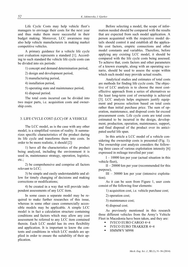
52 K. Jakimovska, I. Gjurkov
Mech. Eng. Sci. J., 32 (1), 51–56 (2014)
Life Cycle Costs may help vehicle fleet’s managers to envisage their costs for the next year and thus make them more successful in their budget making. Moreover, LCC awareness may also help vehicle manufacturers in making market competitive vehicles.
A primary guidance for a vehicle life cycle cost evaluation represents a standard [1]. Accord-ing to such standard the vehicle life cycle costs can be divided into six periods:
1) concept and demand determination period, 2) design and development period, 3) manufacturing period, 4) installation period, 5) operating state and maintenance period, 6) disposal period. The total costs incurred can be divided into
two major parts, i.e. acquisition costs and owner-ship costs.
3. LIFE CYCLE COST (LCC) ОF A VEHICLE
The LCC model, as is the case with any other model, is a simplified version of reality. It summa-rizes specific characteristics of the product during its life cycle and transforms them into costs. In order to be more realistic, it should [2]:
1) have all the characteristics of the product being analyzed, including the environment it is used in, maintenance strategy, operation, logistics, etc.;
2) be comprehensive and comprise all factors relevant to LCC;
3) be simple and easily understandable and al-low for timely changing of decisions and making corrections or modifications;
4) be created in a way that will provide inde-pendent assessments of any LCC item.
In some cases a separate model may be re-quired to make further researches of this issue, whereas in some other cases commercially acces-sible models may be applicable. A simple LCC model is in fact a calculation structure containing conditions and factors which may allow any cost assessment be referred to any LCC item contained therein. Each LCC model has its own flexibility and application. It is important to know the con-tents and conditions in which LCC models are ap-plied in order to ensure the suitability of their ap-plication.
Before selecting a model, the scope of infor-mation needed should be compared with the results that are expected from such model application. A person acquainted with the respective model de-tails should control it and establish all the applica-ble cost factors, empiric connections and other model constants and variables. Therefore, before applying any existing LCC model, it should be compared with the life cycle costs being assessed. To achieve that, costs factors and other parameters of a known example, along with an operating sce-nario, should be used to assess the scope within which such model may provide actual results.
Analytical studies and estimates of total costs are methods for finding life cycle costs. The objec-tive of LCC analysis is to choose the most cost-effective approach from a series of alternatives so the least long-term cost of ownership is achieved [3]. LCC analysis helps engineers justify equip-ment and process selection based on total costs rather than initial purchase price. The sum of op-eration, maintenance, and disposal costs far exceed procurement costs. Life cycle costs are total costs estimated to be incurred in the design, develop-ment, production, operation, maintenance, support, and final disposal of the product over its antici-pated useful life span.
In this article a LCC model of a vehicle con-sidering the ownership costs is presented (Fig. 1). The ownership cost analysis considers the follow-ing three cases of various exploitation intensity [6] expressed in mileage travelled per year:
I – 10000 km per year (actual situation in this vehicle fleet),
II – 20000 km per year (recommended for this purpose),
III – 30000 km per year (intensive exploita-tion).
As it can be seen from Figure 1, user costs consist of the following four elements:
1) acquisition cost, i.e. vehicle purchase cost; 2) operation cost; 3) maintenance cost; 4) disposal cost. As previously mentioned in this research
three different vehicles from the Army’s Vehicle Fleet in Macedonia have been taken, and they are:
IVECO EURO CARGO 4×4 IVECO EURO TRAKKER 4×4 HMMWV M998
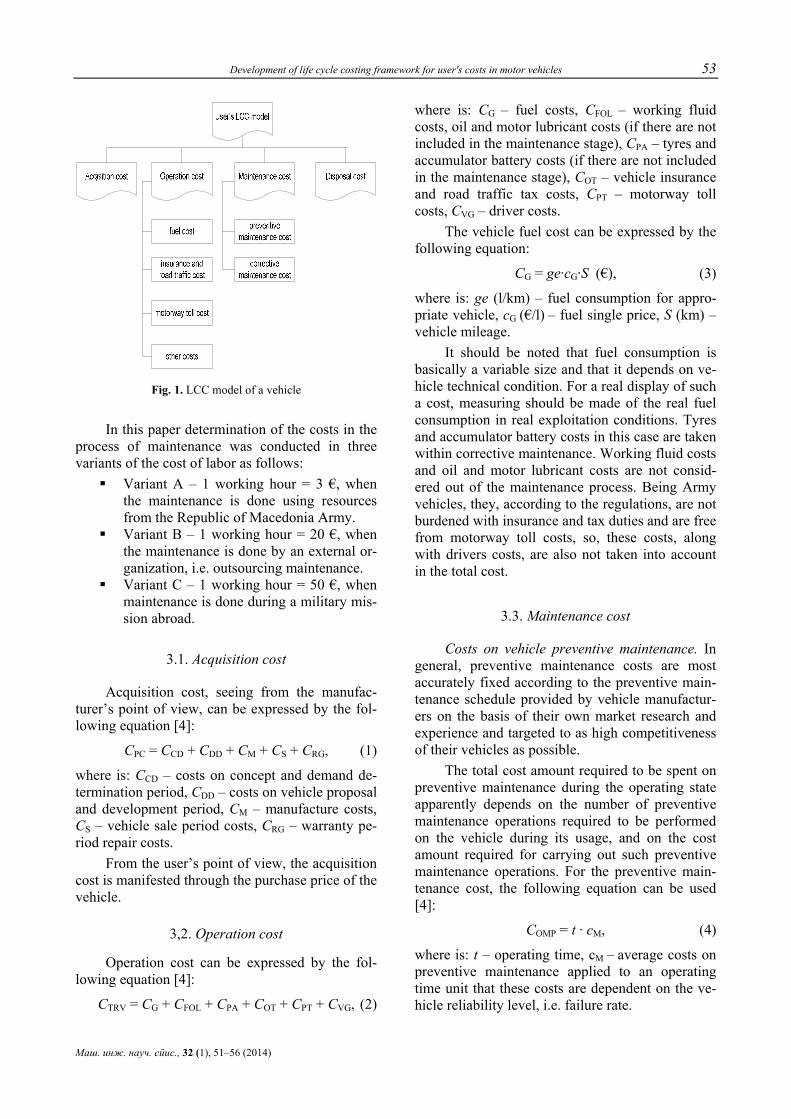
Development of life cycle costing framework for user's costs in motor vehicles 53
Маш. инж. науч. спис., 32 (1), 51–56 (2014)
Fig. 1. LCC model of a vehicle
In this paper determination of the costs in the process of maintenance was conducted in three variants of the cost of labor as follows:
Variant A – 1 working hour = 3 €, when the maintenance is done using resources from the Republic of Macedonia Army.
Variant B – 1 working hour = 20 €, when the maintenance is done by an external or-ganization, i.e. outsourcing maintenance.
Variant C – 1 working hour = 50 €, when maintenance is done during a military mis-sion abroad.
3.1. Acquisition cost
Acquisition cost, seeing from the manufac-turer’s point of view, can be expressed by the fol-lowing equation [4]:
CPC = CCD + CDD + CM + CS + CRG, (1)
where is: CCD – costs on concept and demand de-termination period, CDD – costs on vehicle proposal and development period, CM – manufacture costs, CS – vehicle sale period costs, CRG – warranty pe-riod repair costs.
From the user’s point of view, the acquisition cost is manifested through the purchase price of the vehicle.
3,2. Operation cost
Operation cost can be expressed by the fol-lowing equation [4]:
CTRV = CG + CFOL + CPA + COT + CPT + CVG, (2)
where is: CG – fuel costs, CFOL – working fluid costs, oil and motor lubricant costs (if there are not included in the maintenance stage), CPA – tyres and accumulator battery costs (if there are not included in the maintenance stage), COT – vehicle insurance and road traffic tax costs, CPT – motorway toll costs, CVG – driver costs.
The vehicle fuel cost can be expressed by the following equation:
CG = ge·cG·S (€), (3)
where is: ge (l/km) – fuel consumption for appro-priate vehicle, cG (€/l) – fuel single price, S (km) – vehicle mileage.
It should be noted that fuel consumption is basically a variable size and that it depends on ve-hicle technical condition. For a real display of such a cost, measuring should be made of the real fuel consumption in real exploitation conditions. Tyres and accumulator battery costs in this case are taken within corrective maintenance. Working fluid costs and oil and motor lubricant costs are not consid-ered out of the maintenance process. Being Army vehicles, they, according to the regulations, are not burdened with insurance and tax duties and are free from motorway toll costs, so, these costs, along with drivers costs, are also not taken into account in the total cost.
3.3. Maintenance cost
Costs on vehicle preventive maintenance. In general, preventive maintenance costs are most accurately fixed according to the preventive main-tenance schedule provided by vehicle manufactur-ers on the basis of their own market research and experience and targeted to as high competitiveness of their vehicles as possible.
The total cost amount required to be spent on preventive maintenance during the operating state apparently depends on the number of preventive maintenance operations required to be performed on the vehicle during its usage, and on the cost amount required for carrying out such preventive maintenance operations. For the preventive main-tenance cost, the following equation can be used [4]:
COMP = t · cM, (4)
where is: t – operating time, cM – average costs on preventive maintenance applied to an operating time unit that these costs are dependent on the ve-hicle reliability level, i.e. failure rate.
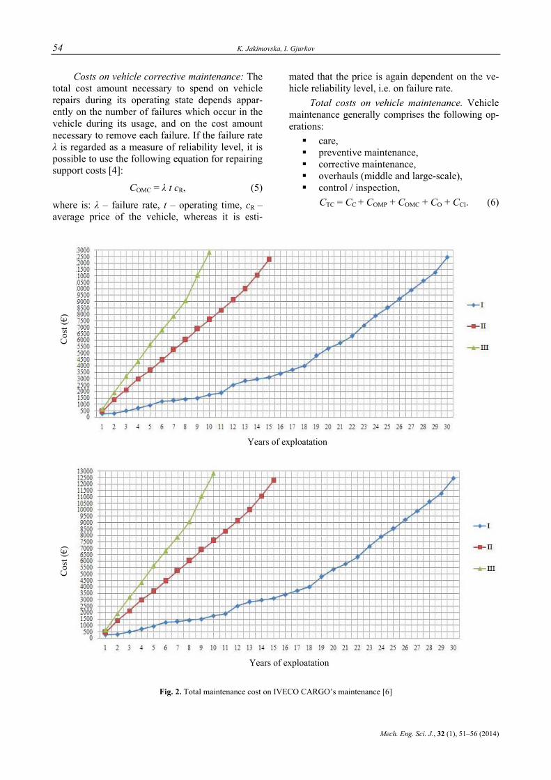
54 K. Jakimovska, I. Gjurkov
Mech. Eng. Sci. J., 32 (1), 51–56 (2014)
Costs on vehicle corrective maintenance: The total cost amount necessary to spend on vehicle repairs during its operating state depends appar-ently on the number of failures which occur in the vehicle during its usage, and on the cost amount necessary to remove each failure. If the failure rate λ is regarded as a measure of reliability level, it is possible to use the following equation for repairing support costs [4]:
COMC = λ t cR, (5)
where is: λ – failure rate, t – operating time, cR – average price of the vehicle, whereas it is esti-
mated that the price is again dependent on the ve-hicle reliability level, i.e. on failure rate.
Total costs on vehicle maintenance. Vehicle maintenance generally comprises the following op-erations:
care, preventive maintenance, corrective maintenance, overhauls (middle and large-scale), control / inspection,
CTC = CC + COMP + COMC + CO + CCI. (6)
Cos
t (€)
Years of exploatation
Cos
t (€)
Years of exploatation
Fig. 2. Total maintenance cost on IVECO CARGO’s maintenance [6]
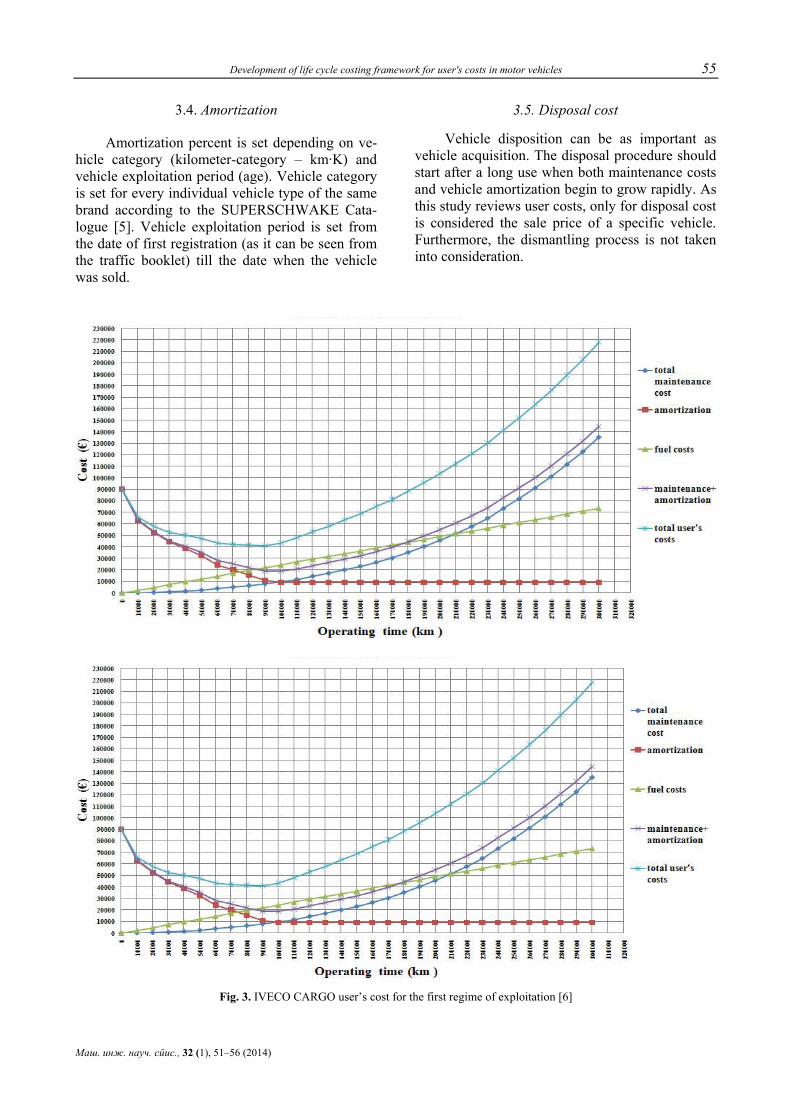
Development of life cycle costing framework for user's costs in motor vehicles 55
Маш. инж. науч. спис., 32 (1), 51–56 (2014)
3.4. Amortization
Amortization percent is set depending on ve-hicle category (kilometer-category – km·K) and vehicle exploitation period (age). Vehicle category is set for every individual vehicle type of the same brand according to the SUPERSCHWAKE Cata-logue [5]. Vehicle exploitation period is set from the date of first registration (as it can be seen from the traffic booklet) till the date when the vehicle was sold.
3.5. Disposal cost
Vehicle disposition can be as important as vehicle acquisition. The disposal procedure should start after a long use when both maintenance costs and vehicle amortization begin to grow rapidly. As this study reviews user costs, only for disposal cost is considered the sale price of a specific vehicle. Furthermore, the dismantling process is not taken into consideration.
Fig. 3. IVECO CARGO user’s cost for the first regime of exploitation [6]

56 K. Jakimovska, I. Gjurkov
Mech. Eng. Sci. J., 32 (1), 51–56 (2014)
4. CONCLUSIONS
The article describes methodology of calcu-lating user costs on any vehicle. To carry out this task successfully, it is necessary to collect and sort data on the occurrence and relevancy of failures, costs on failures removal, preventive maintenance costs and costs on operating state. The developed LCC model on the vehicle user costs includes any influential elements found in the use of vehicles.
This model is easy to understand and allows for relevant corrections and modifications. It has been verified in this research by analyses made on the relevant military vehicles of my country.
Knowledge of the vehicle user costs may help vehicle maintenance engineers to envisage such costs for the next year and thus create their budget more successfully. Moreover, knowledge of such costs may also help vehicle manufacturers be more competitive.
REFERENCES
[1] International Standard, “Dependability management – Part 3: Application guide – Section 3: Life Cycle Costing, IEC 60300-3-3, 2005.
[2] Blanchard, B., Fabricky, W.: Life-Cycle Cost and Eco-nomic Analysis, Prentice Hall, Inc., Englewood Cliffs, NJ, 122–235, 1991.
[3] Barringer, P.: Life Cycle Costs and Good Practices, NPRA Maintenance Conference, USA, 16–26, 1998.
[4] Furch, J.: Determination of vehicle durability time based on life cycle costs and failure intensity, University of De-fence – Brno, Czech Republic, 1–3, 2008.
[5] Schwake Liste, Super Schwake, Band I – 12/06, Eurotaxs-chwake, 1–17, 251–254, 2006.
[6] Jakimovska, K., Research on the user’s costs in motor vehicles life cycle. Master thesis on the Faculty of Me-chanical Engineering, “Ss. Cyril and Methodius” Univer-sity in Skopje, 106–150, 2009.
[7] Blanchard, B., Fabrycky W.: Systems engineering and analysis, Virginia Polytechnic Institute and State Univer-sity, Prentice-Hall, Inc., Englewood Cliffs, N.J., 490–539, 1981.
[8] Barringer, P.: A Life Cycle Cost Summary, International Conference on Maintenance Societies – ICOMS, 1–10, 2003.
[9] Stevanović, I., Stanojević, D., Nedić, A.: Setting the after sales process and quality control at car dealerships to the purpose of increasing clients’ satisfaction, Journal of Ap-plied Engineering Science (Istraživanja i projektovanja za privredu), Vol. 11, No. 2, pp. 81–88 (2013).

Mechanical Engineering – Scientific Journal, Vol. 32, No. 1, pp. 57–63 (2014) CODEN: MINSC5 – 454 In print: ISSN 1857–5293 Received: September 24, 2013 On line: ISSN 1857–9191 Accepted: February 20, 2014 UDC: 004.946
Original scientific paper
COMPARATION OF SEVERAL MODELS FOR INTERACTION IN VIRTUAL REALITY
Filip Popovski, Igor Nedelkovski
Faculty of Technical Sciences, “St Kliment Ohridski” University, Ivo L. Ribar, 7000 Bitola, Republic of Macedonia
A b s t r a c t: Virtual reality is the use of computer technology to create the effect of an interactive 3D world in which the objects have a sense of spatial presence. The primary difference between conventional 3D computer graphics and Virtual Reality is that in Virtual Reality we are working with things instead of pictures of things. In this paper are compared 6 models for simulation scenes in virtual reality and also is made their comparison in terms of features that they offer and the price for their implementation. The purpose of the analysis is to obtain guidance for developing own model for interactive scientific visualization adapted to circumstances in research centers in Republic of Macedonia, which means to be optimized for effective results by using cheap equipment no more than 1000 Euro.
Key words: virtual reality; virtual environments; scientific visualization; computer design; techniques of interaction
СПОРЕДБА НА НЕКОЛКУ МОДЕЛИ ЗА ИНТЕРАКЦИЈА ВО ВИРТУЕЛНА РЕАЛНОСТ
А п с т р а к т: Виртуелната реалност претставува користење на компјутерската технологија за создавање ефект на тридимензионален свет во кој предметите имаат изглед на просторна присутност. Основната разлика помеѓу конвенционалната компјутерска 3Д графика и виртуелната реалност е тоа што во виртуелната реалност работиме со предмети наместо со слики на предмети. Во овој труд се анализирани 6 модели за виртуелна реалност и направена е нивна споредба во однос на карактеристиките коишто ги нудат и цената за нивна имплементација. Целта на анализа-та е да се добијат насоки за развој на сопствен модел за интерактивна научна визуализација, усогласен со приликите во истражувачките центри во Република Македонија, што значи да е оптимиран за добивање ефективни резултати со користење на евтина опрема која би чинела околу 1000 EUR.
Клучни зборови: виртуелна реалност; виртуелна околина; научна визуализација; компјутерски дизајн; техники на интеракција
1. INTRODUCTION
The idea of inserting a man in some imagi-nary the world is very old. Needs for visualization unrealistic, but yet sufficiently realistic environ-ments occurs in the middle of the twentieth cen-tury. First registered attempt that has similarities with modern devices was constructed by Morton Heilig (1926–1997) and was named Sensorama. It was a motorcycle simulator that had a wide range
of stimuli that simulate. For visualization of im-ages it used video projection and for sound it used appropriate audio of motorcycle. It was interesting that this device simulated vibration and even the smell of overheating tyre. In 1960 was designed the first device with built-in display that bring on the head (HMD), and in 1977's was constructed first Data Glove. The early nineties of the last cen-tury marked the development of various devices and software for virtual reality. Today, the applica-
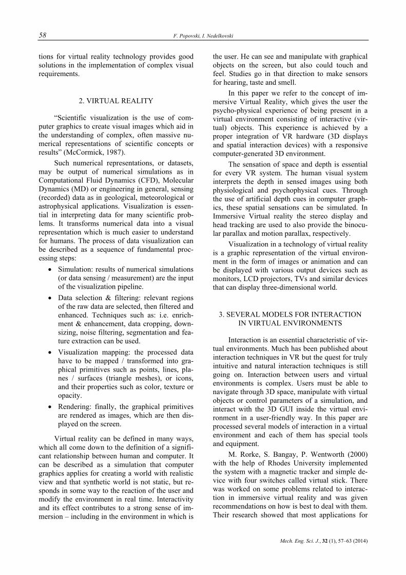
58 F. Popovski, I. Nedelkovski
Mech. Eng. Sci. J., 32 (1), 57–63 (2014)
tions for virtual reality technology provides good solutions in the implementation of complex visual requirements.
2. VIRTUAL REALITY
“Scientific visualization is the use of com-puter graphics to create visual images which aid in the understanding of complex, often massive nu-merical representations of scientific concepts or results” (McCormick, 1987).
Such numerical representations, or datasets, may be output of numerical simulations as in Computational Fluid Dynamics (CFD), Molecular Dynamics (MD) or engineering in general, sensing (recorded) data as in geological, meteorological or astrophysical applications. Visualization is essen-tial in interpreting data for many scientific prob-lems. It transforms numerical data into a visual representation which is much easier to understand for humans. The process of data visualization can be described as a sequence of fundamental proc-essing steps:
• Simulation: results of numerical simulations (or data sensing / measurement) are the input of the visualization pipeline.
• Data selection & filtering: relevant regions of the raw data are selected, then filtered and enhanced. Techniques such as: i.e. enrich-ment & enhancement, data cropping, down-sizing, noise filtering, segmentation and fea-ture extraction can be used.
• Visualization mapping: the processed data have to be mapped / transformed into gra-phical primitives such as points, lines, pla-nes / surfaces (triangle meshes), or icons, and their properties such as color, texture or opacity.
• Rendering: finally, the graphical primitives are rendered as images, which are then dis-played on the screen.
Virtual reality can be defined in many ways, which all come down to the definition of a signifi-cant relationship between human and computer. It can be described as a simulation that computer graphics applies for creating a world with realistic view and that synthetic world is not static, but re-sponds in some way to the reaction of the user and modify the environment in real time. Interactivity and its effect contributes to a strong sense of im-mersion – including in the environment in which is
the user. He can see and manipulate with graphical objects on the screen, but also could touch and feel. Studies go in that direction to make sensors for hearing, taste and smell.
In this paper we refer to the concept of im-mersive Virtual Reality, which gives the user the psycho-physical experience of being present in a virtual environment consisting of interactive (vir-tual) objects. This experience is achieved by a proper integration of VR hardware (3D displays and spatial interaction devices) with a responsive computer-generated 3D environment.
The sensation of space and depth is essential for every VR system. The human visual system interprets the depth in sensed images using both physiological and psychophysical cues. Through the use of artificial depth cues in computer graph-ics, these spatial sensations can be simulated. In Immersive Virtual reality the stereo display and head tracking are used to also provide the binocu-lar parallax and motion parallax, respectively.
Visualization in a technology of virtual reality is a graphic representation of the virtual environ-ment in the form of images or animation and can be displayed with various output devices such as monitors, LCD projectors, TVs and similar devices that can display three-dimensional world.
3. SEVERAL MODELS FOR INTERACTION IN VIRTUAL ENVIRONMENTS
Interaction is an essential characteristic of vir-tual environments. Much has been published about interaction techniques in VR but the quest for truly intuitive and natural interaction techniques is still going on. Interaction between users and virtual environments is complex. Users must be able to navigate through 3D space, manipulate with virtual objects or control parameters of a simulation, and interact with the 3D GUI inside the virtual envi-ronment in a user-friendly way. In this paper are processed several models of interaction in a virtual environment and each of them has special tools and equipment.
M. Rorke, S. Bangay, P. Wentworth (2000) with the help of Rhodes University implemented the system with a magnetic tracker and simple de-vice with four switches called virtual stick. There was worked on some problems related to interac-tion in immersive virtual reality and was given recommendations on how is best to deal with them. Their research showed that most applications for
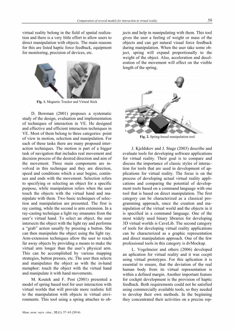
Comparation of several models for interaction in virtual reality 59
Маш. инж. науч. спис., 32 (1), 57–63 (2014)
virtual reality belong in the field of spatial realiza-tion and there is a very little effort to allow users to direct manipulation with objects. The main reasons for this are listed haptic force feedback, equipment for monitoring, precision of devices, etc.
Fig. 1. Magnetic Tracker and Virtual Stick
D. Bowman (2001) proposes a systematic study of the design, evaluation and implementation of techniques of interaction in VE. He designed and effective and efficient interaction techniques in VE. Most of them belong to three categories: point of view in motion, selection and manipulation. For each of these tasks there are many proposed inter-action techniques. The motion is part of a bigger task of navigation that includes real movement and decision process of the desired direction and aim of the movement. Three main components are in-volved in this technique and they are direction, speed and conditions which a user begins, contin-ues and ends with the movement. Selection refers to specifying or selecting an object for a specific purpose, while manipulation refers when the user touch the objects with the virtual hand and ma-nipulate with them. Two basic techniques of selec-tion and manipulation are presented. The first is ray casting, while the second is arm extension. In a ray-casting technique a light ray emanates from the user’s virtual hand. To select an object, the user intersects the object with the light ray and performs a “grab” action usually by pressing a button. She can then manipulate the object using the light ray. Arm-extension techniques allow the user to reach far away objects by providing a means to make the virtual arm longer than the user’s physical arm. This can be accomplished by various mapping strategies, button presses, etc. The user then selects and manipulates the object as with the in-hand metaphor: touch the object with the virtual hand and manipulate it with hand movements.
M. Koutek and F. Post (2001) presented a model of spring based tool for user interaction with virtual worlds that will provide more realistic fell to the manipulation with objects in virtual envi-ronments. This tool using a spring attaches to ob-
jects and help in manipulating with them. This tool gives the user a feeling of weight or mass of the objects and can get natural visual force feedback during manipulation. When the user take some ob-ject, spring will expand proportionally to the weight of the object. Also, acceleration and decel-eration of the movement will effect on the visible length of the spring.
Fig. 2. Spring-based manipulation tool
J. Kjeldskov and J. Stage (2003) describe and evaluate tools for developing software applications for virtual reality. Their goal is to compare and discuss the importance of classic styles of interac-tion for tools that are used in development of ap-plications for virtual reality. The focus is on the process of developing actual virtual reality appli-cations and comparing the potential of develop-ment tools based on a command language with one tool that is based on direct manipulation. The first category can be characterized as a classical pro-gramming approach, since the creation and ma-nipulation of the virtual world and the objects in it is specified in a command language. One of the most widely used binary libraries for developing 3D virtual worlds is CaveLib. The second category of tools for developing virtual reality applications can be characterized as a graphic representation and direct manipulation approach. One of the few professional tools in this category is dvMockup.
L. Vogelmeier and others (2006) developed an aplication for virtual reality and it was cocpit using virtual prototypes. For this aplication it is essential to ensure, that the deviation of the real human body from its virtual representation is within a defined margin. Another important feature for cockpit development is the provision of haptic feedback. Both requirements could not be satisfied using commercially available tools, so they needed to develop their own methods. In the beginning they concentrated their activities on a precise rep-
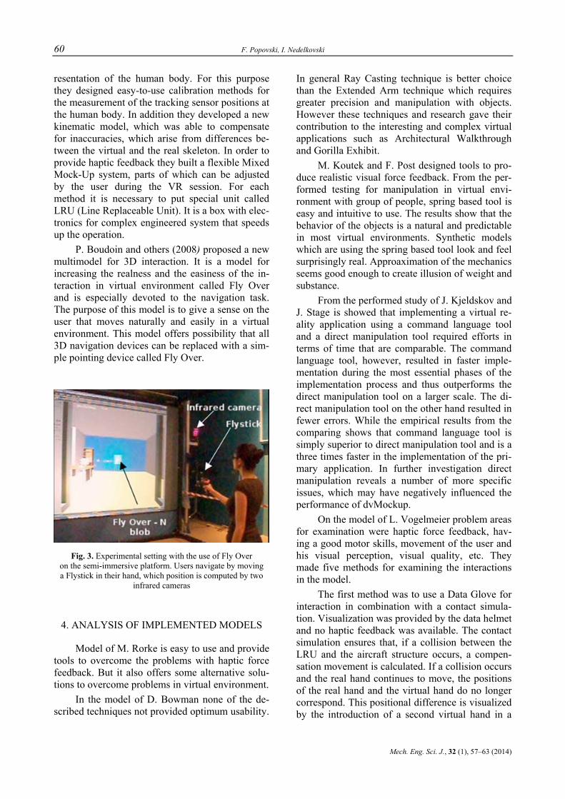
60 F. Popovski, I. Nedelkovski
Mech. Eng. Sci. J., 32 (1), 57–63 (2014)
resentation of the human body. For this purpose they designed easy-to-use calibration methods for the measurement of the tracking sensor positions at the human body. In addition they developed a new kinematic model, which was able to compensate for inaccuracies, which arise from differences be-tween the virtual and the real skeleton. In order to provide haptic feedback they built a flexible Mixed Mock-Up system, parts of which can be adjusted by the user during the VR session. For each method it is necessary to put special unit called LRU (Line Replaceable Unit). It is a box with elec-tronics for complex engineered system that speeds up the operation.
P. Boudoin and others (2008) proposed a new multimodel for 3D interaction. It is a model for increasing the realness and the easiness of the in-teraction in virtual environment called Fly Over and is especially devoted to the navigation task. The purpose of this model is to give a sense on the user that moves naturally and easily in a virtual environment. This model offers possibility that all 3D navigation devices can be replaced with a sim-ple pointing device called Fly Over.
Fig. 3. Experimental setting with the use of Fly Over on the semi-immersive platform. Users navigate by moving a Flystick in their hand, which position is computed by two
infrared cameras
4. ANALYSIS OF IMPLEMENTED MODELS
Model of M. Rorke is easy to use and provide tools to overcome the problems with haptic force feedback. But it also offers some alternative solu-tions to overcome problems in virtual environment.
In the model of D. Bowman none of the de-scribed techniques not provided optimum usability.
In general Ray Casting technique is better choice than the Extended Arm technique which requires greater precision and manipulation with objects. However these techniques and research gave their contribution to the interesting and complex virtual applications such as Architectural Walkthrough and Gorilla Exhibit.
M. Koutek and F. Post designed tools to pro-duce realistic visual force feedback. From the per-formed testing for manipulation in virtual envi-ronment with group of people, spring based tool is easy and intuitive to use. The results show that the behavior of the objects is a natural and predictable in most virtual environments. Synthetic models which are using the spring based tool look and feel surprisingly real. Approaximation of the mechanics seems good enough to create illusion of weight and substance.
From the performed study of J. Kjeldskov and Ј. Stage is showed that implementing a virtual re-ality application using a command language tool and a direct manipulation tool required efforts in terms of time that are comparable. The command language tool, however, resulted in faster imple-mentation during the most essential phases of the implementation process and thus outperforms the direct manipulation tool on a larger scale. The di-rect manipulation tool on the other hand resulted in fewer errors. While the empirical results from the comparing shows that command language tool is simply superior to direct manipulation tool and is a three times faster in the implementation of the pri-mary application. In further investigation direct manipulation reveals a number of more specific issues, which may have negatively influenced the performance of dvMockup.
On the model of L. Vogelmeier problem areas for examination were haptic force feedback, hav-ing a good motor skills, movement of the user and his visual perception, visual quality, etc. They made five methods for examining the interactions in the model.
The first method was to use a Data Glove for interaction in combination with a contact simula-tion. Visualization was provided by the data helmet and no haptic feedback was available. The contact simulation ensures that, if a collision between the LRU and the aircraft structure occurs, a compen-sation movement is calculated. If a collision occurs and the real hand continues to move, the positions of the real hand and the virtual hand do no longer correspond. This positional difference is visualized by the introduction of a second virtual hand in a
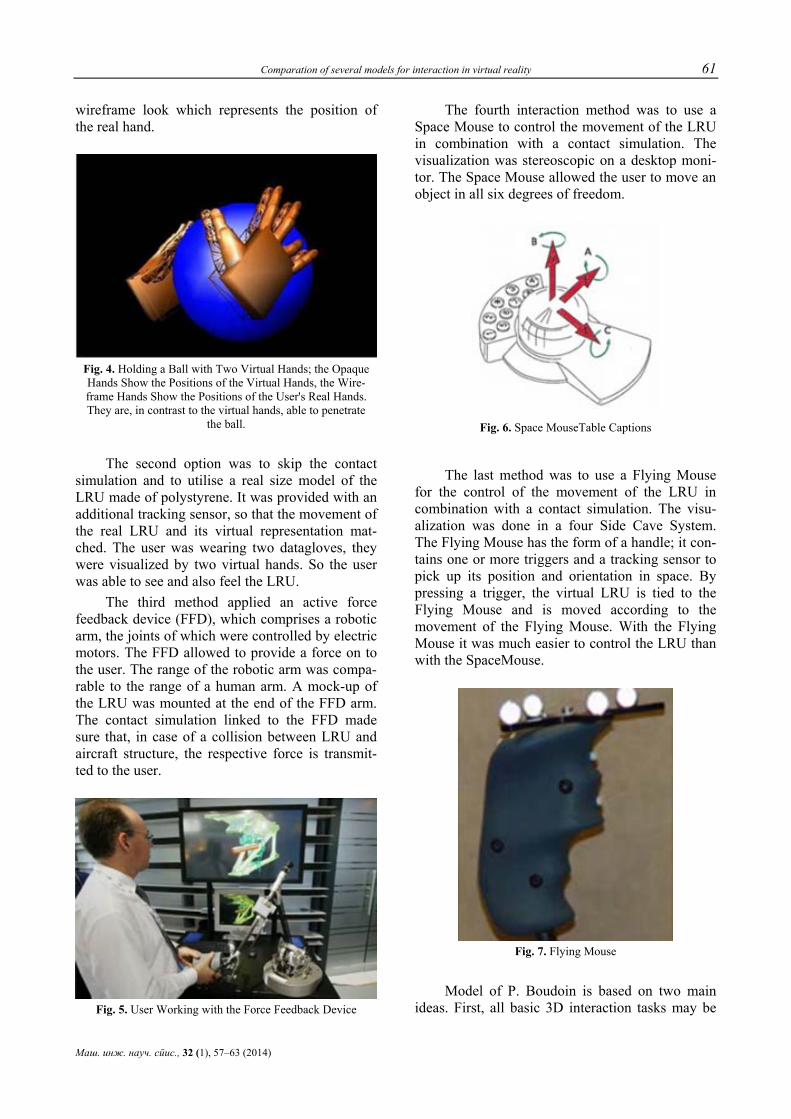
Comparation of several models for interaction in virtual reality 61
Маш. инж. науч. спис., 32 (1), 57–63 (2014)
wireframe look which represents the position of the real hand.
Fig. 4. Holding a Ball with Two Virtual Hands; the Opaque Hands Show the Positions of the Virtual Hands, the Wire-frame Hands Show the Positions of the User's Real Hands. They are, in contrast to the virtual hands, able to penetrate
the ball.
The second option was to skip the contact simulation and to utilise a real size model of the LRU made of polystyrene. It was provided with an additional tracking sensor, so that the movement of the real LRU and its virtual representation mat-ched. The user was wearing two datagloves, they were visualized by two virtual hands. So the user was able to see and also feel the LRU.
The third method applied an active force feedback device (FFD), which comprises a robotic arm, the joints of which were controlled by electric motors. The FFD allowed to provide a force on to the user. The range of the robotic arm was compa-rable to the range of a human arm. A mock-up of the LRU was mounted at the end of the FFD arm. The contact simulation linked to the FFD made sure that, in case of a collision between LRU and aircraft structure, the respective force is transmit-ted to the user.
Fig. 5. User Working with the Force Feedback Device
The fourth interaction method was to use a Space Mouse to control the movement of the LRU in combination with a contact simulation. The visualization was stereoscopic on a desktop moni-tor. The Space Mouse allowed the user to move an object in all six degrees of freedom.
Fig. 6. Space MouseTable Captions
The last method was to use a Flying Mouse for the control of the movement of the LRU in combination with a contact simulation. The visu-alization was done in a four Side Cave System. The Flying Mouse has the form of a handle; it con-tains one or more triggers and a tracking sensor to pick up its position and orientation in space. By pressing a trigger, the virtual LRU is tied to the Flying Mouse and is moved according to the movement of the Flying Mouse. With the Flying Mouse it was much easier to control the LRU than with the SpaceMouse.
Fig. 7. Flying Mouse
Model of P. Boudoin is based on two main ideas. First, all basic 3D interaction tasks may be
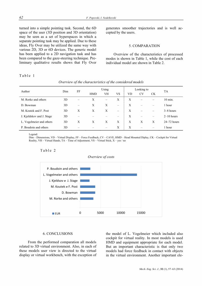
62 F. Popovski, I. Nedelkovski
Mech. Eng. Sci. J., 32 (1), 57–63 (2014)
turned into a simple pointing task. Second, the 6D space of the user (3D position and 3D orientation) may be seen as a set of hyperspaces in which a separate pointing task may be applied. Due to these ideas, Fly Over may be utilized the same way with various 2D, 3D or 6D devices. The generic model has been applied to a 2D navigation task and has been compared to the gaze-steering technique. Pre-liminary qualitative results shows that Fly Over
generates smoother trajectories and is well ac-cepted by the users.
5. COMPARATION
Overview of the characteristics of processed modes is shown in Table 1, while the cost of each individual model are shown in Table 2.
T a b l e 1
Overview of the characteristics of the considered models
Using Looking to Author Dim FF
HMD VH VS VD CV CK TA
M. Rorke and others 3D – X – Х Х – – 10 min.
D. Bowman 3D – Х Х – Х – – 1 hour
M. Koutek and F. Post 3D Х Х X – Х – – 3–8 hours
J. Kjeldskov and J. Stage 3D – – – – Х – – 2–10 hours
L. Vogelmeier and others 3D Х Х Х Х Х Х Х 24–72 hours
P. Boudoin and others 3D – – – Х Х – – 1 hour
Legend: Dim – Dimensions, VD – Virtual Display, FF – Force Feedback, CV – CAVE, HMD – Head Mounted Diplay, CK – Cockpit for Virtual Reality, VH – Virtual Hands, TA – Time of Adjustment, VS – Virtual Stick, Х – yes / no
T a b l e 2
Overview of costs
0 5000 10000 15000
M. Rorke and others
D. Bowman
M. Koutek и F. Post
J. Kjeldsov и J. Stage
L. Vogelmeier and others
P. Boudoin and others
EUR
6. CONCLUSIONS
From the performed comparation all models related to 3D virtual environment. Also, in each of these models user view is directed to the virtual display or virtual workbench, with the exception of
the model of L. Vogelmeier which included also cockpit for virtual reality. In most models is used HMD and equipment appropriate for each model. But an important characteristic is that only two models had force feedback in contact with objects in the virtual environment. Another important ele-

Comparation of several models for interaction in virtual reality 63
Маш. инж. науч. спис., 32 (1), 57–63 (2014)
ment in these models is a time of adaptation by the user. From performed analysis model of M. Rorke is the easiest for using and can be used after 10 minutes of exercise. All models have a similar price in the market which is around 3000 EUR ex-cluding model of L. Vogelmeier which is very ex-pensive due to the complexity of the system and the high performance it has.
At te Faculty of Technical Sciences in Bitola in progress is development a model for interactive scientific visualization that will be based on the following principles:
• user friendly interface; • using open soure libraries; • using computer monitor or LED TV; • unexpensive accessories needed for virtual
navigation (HMD, trackball, virtual stick). The same model compared with analyzed is
expected to have the following advantages: • to enable work on any computer that sup-
ports CAD software who can run interactive scientific visualization;
• it will be a low cost about 1,000 EUR;
• it will give a contribution to the field of in-teractive scientific visualization as a tool for a large number of users which are not spe-cialized in the field of engineering technol-ogy and virtual reality.
REFERENCES
[1] D. Bowman, L. Hodges: An Evaluation of Techniques for Grabbing and Manipulating Remote Objects in Im-mersive Virtual Environments, Proceedings of the ACM Symposium on Interactive 3D Graphics, New York, 1997.
[2] D. Bowman, D. Koller, L. Hodges: Travel in Immersive Virtual Environments: An Evaluation of Viewpoint Mo-tion Control Techniques, Proceedings of Virtual Reality Annual International Symposium , 1997.
[3] M. H. Hougaard, N. Kolbe, F. N. : Comparison of Tools for Developing Virtual Reality Application, Intermedia, Aalborg University, 2001.
[4] J. Kjeldskov, J. Stage: Interaction Styles in Development Tools for Virtual Reality Applications, Springer-Verlag, Berlin, 2003.
[5] P. Boudoin, S, Otmane, M. Mallem: Design of a 3D Navi-gation Technique Supporting VR Interaction, CISA, An-naba, Algeria, 2008.
[6] L. Vogelmeier, H. Neujahr, P. Sandl:: Interaction Meth-ods for Virtual Reality Applications, Virtual Media for Military Applications, West Point, NY, 2006.

Mechanical Engineering – Scientific Journal, Vol. 32, No. 1, pp. 65–69 (2014) CODEN: MINSC5 – 455 In print: ISSN 1857–5293 Received: October 14, 2013 On line: ISSN 1857–9191 Accepted: February 20, 2014 UDC: 621.224:681.511.4
Original scientific paper
COMPARISON OF SIMULATED AND MEASURED RESPONSE OF LOAD REJECTION ON A HYDRO POWER PLANT MODEL
WITH MIXED MODE NONLINEAR CONTROLLER
Darko Babunski, Atanasko Tuneski, Emil Zaev
"Ss. Cyril and Methodius" University in Skopje, Faculty of Mechanical Engineering, Karpoš II bb, P.O. box 464, 1001 Skopje, Republic of Macedonia,
A b s t r a c t: Revised Hydro Power Plant model of the IEEE working group recommended converted to state space model is used for simulation of transient response of hydro turbine, and verification was made using measure-ments of transients from real Hydro Power Plant (HPP). Nonlinear mixed model controller was designed and imple-mented into complete HPP simulation model and compared with PID with real parameters used in HPP, and with ad-justed PID parameters with consideration of smallest frequency error. Verification of performance of the model was made comparing model response with measured load rejection, which is worst case of HPP operation.
Key words: hydro power plant; hydro turbine; nonlinear control; controller
СПОРЕДБА НА СИМУЛИРАН И ИЗМЕРЕН ОДЗИВ ПРИ ОДБИВАЊЕ НА ОПТОВАРУВАЊЕ НА МОДЕЛ НА ХИДРОЕЛЕКТРИЧНА ПОСТРОЈКА
СО КОМБИНИРАН НЕЛИНЕАРЕН УПРАВУВАЧ
А п с т р а к т: За симулација на однесувањето на хидроелектричните постројки (ХЕП) во екстремни ситуации како што се побег, одбивање на оптоварување и слично, се користи ревидираниот модел на работ-ната група на IEEE, приведен во простор на состојба и верифициран преку експериментални мерења на преодните карактеристики на ХЕП. Проектиран е нов комбиниран нелинеарен управувач и е имплементиран во верифицираниот модел на ХЕП. Одзивите на така дефинираниот систем се споредени со реално измерени-те одзиви на ХЕП, како и со симулации на модели на ХЕП кои користат два типа на ПИД-управување
Клучни зборови: хидроенергетска постројка; хидраулична турбина; нелинеарно управување; управувач
1. INTRODUCTION
Hydro Turbine is highly nonlinear device which behavior is highly unpredictable and varying with change of network load. Because of that, use of linearized models for simulation of dynamic response characteristics of Hydro Turbine is not recommended. In this paper revised model of the IEEE working group [1] recommended is used for simulation of transient response of hydro turbine, and verification was made using measurements of transients from real Hydro Power Plant (HPP). Af-ter that, nonlinear mixed model controller was de-signed and implemented into complete HPP simu-
lation model. Verification of performance of the model was made comparing model response with measured load rejection, which is worst case of HPP operation. Simulation response was compared to simulation model with PID with real parameters used in HPP, and with adjusted PID parameters with consideration of smallest frequency error.
2. NONLINEAR HYDRO POWER PLANT MODEL WITH SURGE TANK
Recommended models for simulation of hy-dro turbine [1, 2] are mainly nonlinear models for hydro turbine with tunnel, surge tank and penstock,
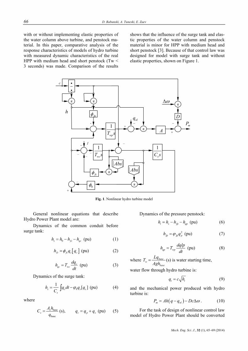
66 D. Babunski, A. Tuneski, E. Zaev
Mech. Eng. Sci. J., 32 (1), 65–69 (2014)
with or without implementing elastic properties of the water column above turbine, and penstock ma-terial. In this paper, comparative analysis of the response characteristics of models of hydro turbine with measured dynamic characteristics of the real HPP with medium head and short penstock (Tw < 3 seconds) was made. Comparison of the results
shows that the influence of the surge tank and elas-tic properties of the water column and penstock material is minor for HPP with medium head and short penstock [3]. Because of that control law was designed for model with surge tank and without elastic properties, shown on Figure 1.
Fig. 1. Nonlinear hydro turbine model
General nonlinear equations that describe Hydro Power Plant model are:
Dynamics of the common conduit before surge tank:
0s fc qch h h h= − − (pu) (1)
[ ]fc fc c ch q qφ= (pu) (2)
cqc wc
dqh Tdt
= (pu) (3)
Dynamics of the surge tank:
01 [ ]s s s s
s
h q dt q qC
ϕ= −∫ (pu) (4)
where
base
base
ss
A hCq
= (s), c p sq q q= + (pu) (5)
Dynamics of the pressure penstock:
t s fp qph h h h= − − (pu) (6)
2fp fp ph qϕ= (pu) (7)
qp wpdqlph Tdt
= (pu) (8)
where basew
base
LqTAgh
= (s) is water starting time,
water flow through hydro turbine is:
t tq c h= (9)
and the mechanical power produced with hydro turbine is: ( )m nlP Ah q q Dc ω= − − ∆ . (10)
For the task of design of nonlinear control law model of Hydro Power Plant should be converted
nlq
–
–
h
c
+
+
1
fpφ
πtA
D
mP
ω∆
1
sC s
1
wpT s
ii
1
wcT s
Abs
fcφ Abs
0φ –
– –
–
–
π
π
π
π π
- –
+
–
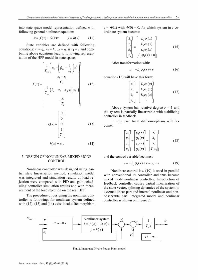
Comparison of simulated and measured response of load rejection on a hydro power plant model with mixed mode nonlinear controller 67
Маш. инж науч. спис., 32 (1), 65–69 (2014)
into state space model representation defined with following general nonlinear equation:
( ) ( )x f x G x u= + ( )y h x= (11)
State variables are defined with following equations: x1 = qt, x2 = hs, x3 = qc и x4 = c and com-bining above equations lead to following represen-tation of the HPP model in state space:
[ ]( )
22 12
4
3 1
2 3 3
4
1 1
( )1
fpwp
s
o fcws
g
x xT x
x xCf x
h x x xT
xT
φ
φ
⎡ ⎤⎛ ⎞⎛ ⎞− +⎢ ⎥⎜ ⎟⎜ ⎟⎜ ⎟⎢ ⎝ ⎠ ⎥⎝ ⎠
⎢ ⎥−⎢ ⎥⎢ ⎥= ⎢ ⎥⎢ ⎥− −⎢ ⎥⎢ ⎥⎢ ⎥−⎢ ⎥⎣ ⎦
(12)
000( )1
g
g x
T
⎡ ⎤⎢ ⎥⎢ ⎥⎢ ⎥=⎢ ⎥⎢ ⎥⎢ ⎥⎣ ⎦
(13)
4( )h x x= . (14)
3. DESIGN OF NONLINEAR MIXED MODE CONTROL
Nonlinear controller was designed using par-tial state linearization method, simulation model was integrated and simulation results of load re-jection were compared with PID and gain sched-uling controller simulation results and with meas-urement of the load rejection on the real HPP.
The procedure of designing the nonlinear con-troller is following: for nonlinear system defined with (12), (13) and (14) exist local diffeomorphism
z = Ф(x) with Ф(0) = 0, for which system in z co-ordinate system become:
11
22
33
44
( )( )( )
( ) u
f
f
f
f
L xzL xzL xz
L xz
ϕϕϕ
ϕ
⎡ ⎤⎡ ⎤⎢ ⎥⎢ ⎥⎢ ⎥⎢ ⎥ =⎢ ⎥⎢ ⎥⎢ ⎥⎢ ⎥ +⎢ ⎥⎣ ⎦ ⎣ ⎦
(15)
After transformation with:
4 ( )fu L x vϕ= − + (16)
еquation (15) will have this form:
1 1
2 2
3 3
4
( )( )( )
f
f
f
z L xz L xz L xz v
ϕϕϕ
⎡ ⎤ ⎡ ⎤⎢ ⎥ ⎢ ⎥⎢ ⎥ ⎢ ⎥=⎢ ⎥ ⎢ ⎥⎢ ⎥ ⎢ ⎥
⎣ ⎦⎣ ⎦
(17)
Above system has relative degree r = 1 and the system is partially linearizable with stabilizing controller in feedback.
In this case local diffeomorphism will be-come:
11 1
22 2
33 3
44 4
( )( )( )( ) g
xz xxz xxz x
T xz x
ϕϕϕϕ
⎡ ⎤⎡ ⎤ ⎡ ⎤⎢ ⎥⎢ ⎥ ⎢ ⎥⎢ ⎥⎢ ⎥ ⎢ ⎥= =⎢ ⎥⎢ ⎥ ⎢ ⎥⎢ ⎥⎢ ⎥ ⎢ ⎥⎢ ⎥⎣ ⎦ ⎣ ⎦ ⎣ ⎦
(18)
and the control variable becomes:
4 4( )fu L x v x vϕ= − + = + (19)
Nonlinear control law (19) is used in parallel with conventional PI controller and thus became mixed mode nonlinear controller. Introduction of feedback controller causes partial linearization of the state vector, splitting dynamics of the system to external linear part and internal nonlinear and non-observable part. Integrated model and nonlinear controller is shown on Figure 2.
Fig. 2. Integrated Hydro Power Plant model
+
-
1
mT s
D
Controller refω Nonlinear system
( ) ( )x f x G x u= +
( )y h x=
mP
2xlP
+
- ω
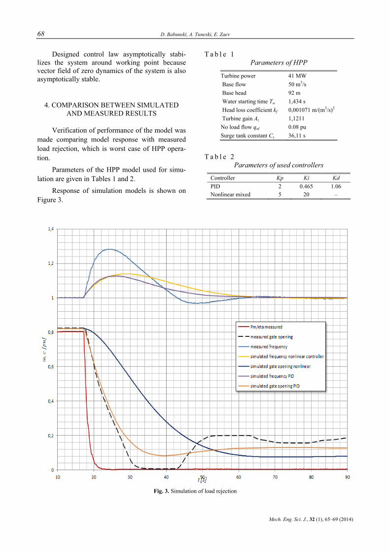
68 D. Babunski, A. Tuneski, E. Zaev
Mech. Eng. Sci. J., 32 (1), 65–69 (2014)
Designed control law asymptotically stabi-lizes the system around working point because vector field of zero dynamics of the system is also asymptotically stable.
4. COMPARISON BETWEEN SIMULATED AND MEASURED RESULTS
Verification of performance of the model was made comparing model response with measured load rejection, which is worst case of HPP opera-tion.
Parameters of the HPP model used for simu-lation are given in Tables 1 and 2.
Response of simulation models is shown on Figure 3.
T a b l e 1 Parameters of HPP
Turbine power 41 MW Base flow 50 m3/s Base head 92 m Water starting time Tw 1,434 s Head loss coefficient kf 0,001071 m/(m3/s)2
Turbine gain At 1,1211 No load flow qnl 0.08 pu Surge tank constant Cs 36,11 s
T a b l e 2 Parameters of used controllers
Controller Kp Ki Kd PID 2 0.465 1.06 Nonlinear mixed 5 20 –
Fig. 3. Simulation of load rejection

Comparison of simulated and measured response of load rejection on a hydro power plant model with mixed mode nonlinear controller 69
Маш. инж науч. спис., 32 (1), 65–69 (2014)
5. CONCLUSIONS
Comparisons of simulation and measured re-sults show that nonlinear controller have robust response, increased gain and phase margin in com-parison with linear control laws, although all con-trol laws have satisfactory response for load rejec-tion on modeled HPP. General conclusion is that for HPP with medium head and short penstock, where effects of surge tank and elastic characteris-tics are minor, careful adjustment of controller pa-rameters is of greater importance that used control law, although nonlinear control law show more robust and slower response with large load change.
REFERENCES
[1] IEEE working group report: Hydraulic turbine and turbine control models for system dynamic studies, IEEE Trans-actions on Power Systems, Vol. 7, No. 1, pp. 167–179 (1992).
[2] Е. De Jaeger, N. Janssens, B. Malfliet, F. Van De Meule-broeke: Hydro turbine model for system dynamic studies. IEEE Transactions on Power Systems, Vol. 9, No 4, pp. 1709–1715 (1994).
[3] D. Babunski, A. Tuneski: Control System Design of Hy-draulic Turbine-Governor, Proceedings of the 11th IEEE International Conference on Emerging Technologies and Factory Automation – ETFA, pp 118–124, Prague, Czech Republic, 2006.
Mechanical Engineering – Scientific Journal, Vol. 32, No. 1, pp. 71–79 (2014) CODEN: MINSC5 – 456 In print: ISSN 1857–5293 Received: March 19, 2013 On line: ISSN 1857–9191 Accepted: April 20, 2014 UDC: 621.645.036:331.454]:681.518
Original scientific paper
ADVANCED EVACUATION MODEL MANAGED THROUGH FUZZY LOGIC DURING AN ACCIDENT IN LNG TERMINAL
Goran Stanković, Stojan Petelin, Marko Perkovič, Peter Vidmar
Faculty for Maritime Studies and Transport, University of Ljubljana, Pot pomorščakov 4, 6320 Portorož, Republic of Slovenia
A b s t r a c t: Evacuation of people located inside the enclosed area of an LNG terminal is a complex problem, especially considering that accidents involving LNG are potentially very hazardous. In order to create an evacuation model managed through fuzzy logic, extensive influence must be generated from safety analyses. A very important moment in the optimal functioning of an evacuation model is the creation of a database which incorporates all input indicators. The output result is the creation of a safety evacuation route which is active at the moment of the accident.
Key words: evacuation model; risk analysis; fuzzy logic; LNG terminal
NAPREDEN EVAKUACIONEN MODEL UPRAVUVAN PREKU FUZZY-LOGIKA PRI NEЗGODA VO TERMINAL ZA TE^EN PRIRODEN GAS
А п с т р а к т: Евакуацијата на луѓето кои се наоѓаат внатре во ограден простор од терминал за течен природен гас (ТПГ) претставува комплексен проблем имајќи предвид дека незгодите со ТПГ се потенцијално многу опасни. За да се изработи евакуационен модел управуван преку Fuzzy-логика, големо влијание имаат спроведените безбедносни анализи. За оптимално функционирање на евакуациониот модел од голема важност е креирањето на база на податоци која ќе ги содржи сите влезни податоци. Краен излезен резултат е креирање на безбедна евакуациона рута која е активна во моментот на незгодата.
Клучни зборови: евакуационен модел; безбедносни анализи; fuzzy-логика; терминал за ТПГ
1. INTRODUCTION
Due to the ever increasing call for energy in the world, there is more and more need to use natu-ral gas as an energy source and hence the need to open new Liquid Natural Gas (LNG) terminals as shipment by sea is inevitable. Basic information regarding LNG terminals is the capacity and num-ber of LNG storage tanks as well as the size and the capacity of the tankers which carry out the transport to the terminal. The potential hazard as-sociated with LNG mainly comes from the possi-bility of an accident with consequences generated by LNG leakage. In such situations, a very possible occurrence is fire and thermal radiation. If the events lead to leakage of a greater quantity of LNG
– into a pool - a cloud is created due to the evapo-ration which contains natural gas, water, steam and air. Due to its weight, the cloud, being heavier than the air, remains at the surface of the earth. The evaporated natural gas may be significantly influ-enced by the atmospheric conditions and the geo-graphic-topographic features of the terrain. The cloud shifts according to the direction of the wind, while the speed of the wind additionally effects the mixing of the natural gas with the air. This mixture is flammable when the concentration of the natural gas in the air ranges between 5% and 15%. The dispersion of the cloud represents a danger to peo-ple, which is increased in the case of flammability. The rapid evacuation of people in such a situation is essential.
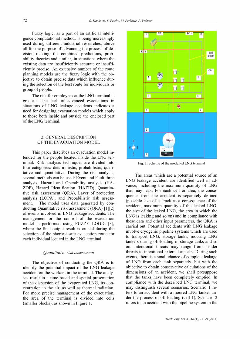
72 G. Stanković, S. Petelin, M. Perkovič, P. Vidmar
Mech. Eng. Sci. J., 32 (1), 71–79 (2014)
Fuzzy logic, as a part of an artificial intelli-gence computational method, is being increasingly used during different industrial researches, above all for the purpose of advancing the process of de-cision making, the combined predictions, prob-ability theories and similar, in situations where the existing data are insufficiently accurate or insuffi-ciently precise. An extensive number of the route planning models use the fuzzy logic with the ob-jective to obtain precise data which influence dur-ing the selection of the best route for individuals or group of people.
The risk for employees at the LNG terminal is greatest. The lack of advanced evacuations in situations of LNG leakage accidents indicates a need for designing evacuation models which apply to those both inside and outside the enclosed part of the LNG terminal.
2. GENERAL DESCRIPTION OF THE EVACUATION MODEL
This paper describes an evacuation model in-tended for the people located inside the LNG ter-minal. Risk analysis techniques are divided into four categories: deterministic, probabilistic, quali-tative and quantitative. During the risk analysis, several methods can be used: Event and Fault three analysis, Hazard and Operability analysis (HA-ZOP), Hazard Identification (HAZID), Quantita-tive risk assessment (QRA), Layer of protection analysis (LOPA), and Probabilistic risk assess-ment. The model uses data generated by con-ducting Quantitative risk assessment (QRA) [1][2] of events involved in LNG leakage accidents. The management or the control of the evacuation model is performed using FUZZY LOGIC [3], where the final output result is crucial during the selection of the shortest safe evacuation route for each individual located in the LNG terminal.
Quantitative risk assessment
The objective of conducting the QRA is to identify the potential impact of the LNG leakage accident on the workers in the terminal. The analy-ses result in a time-based and spatial presentation of the dispersion of the evaporated LNG, its con-centration in the air, as well as thermal radiation. For more precise management of the evacuation, the area of the terminal is divided into cells (smaller blocks), as shown in Figure 1.
Fig. 1. Scheme of the modelled LNG terminal
The areas which are a potential source of an LNG leakage accident are identified well in ad-vance, including the maximum quantity of LNG that may leak. For each cell or area, the conse-quence from the accident is separately defined (possible size of a crack as a consequence of the accident, maximum quantity of the leaked LNG, the size of the leaked LNG, the area in which the LNG is leaking and so on) and in compliance with these data and other input parameters, the QRA is carried out. Potential accidents with LNG leakage involve cryogenic pipeline systems which are used to transport LNG, storage tanks, mooring LNG tankers during off-loading in storage tanks and so on. Intentional threats may range from insider threats to intentional external attacks. During such events, there is a small chance of complete leakage of LNG from each tank separately, but with the objective to obtain conservative calculations of the dimensions of an accident, we shall presuppose that the tanks have been completely emptied. In compliance with the described LNG terminal, we may distinguish several scenarios. Scenario 1 re-fers to an accident with a moored LNG tanker un-der the process of off-loading (cell 1), Scenario 2 refers to an accident with the pipeline system in the
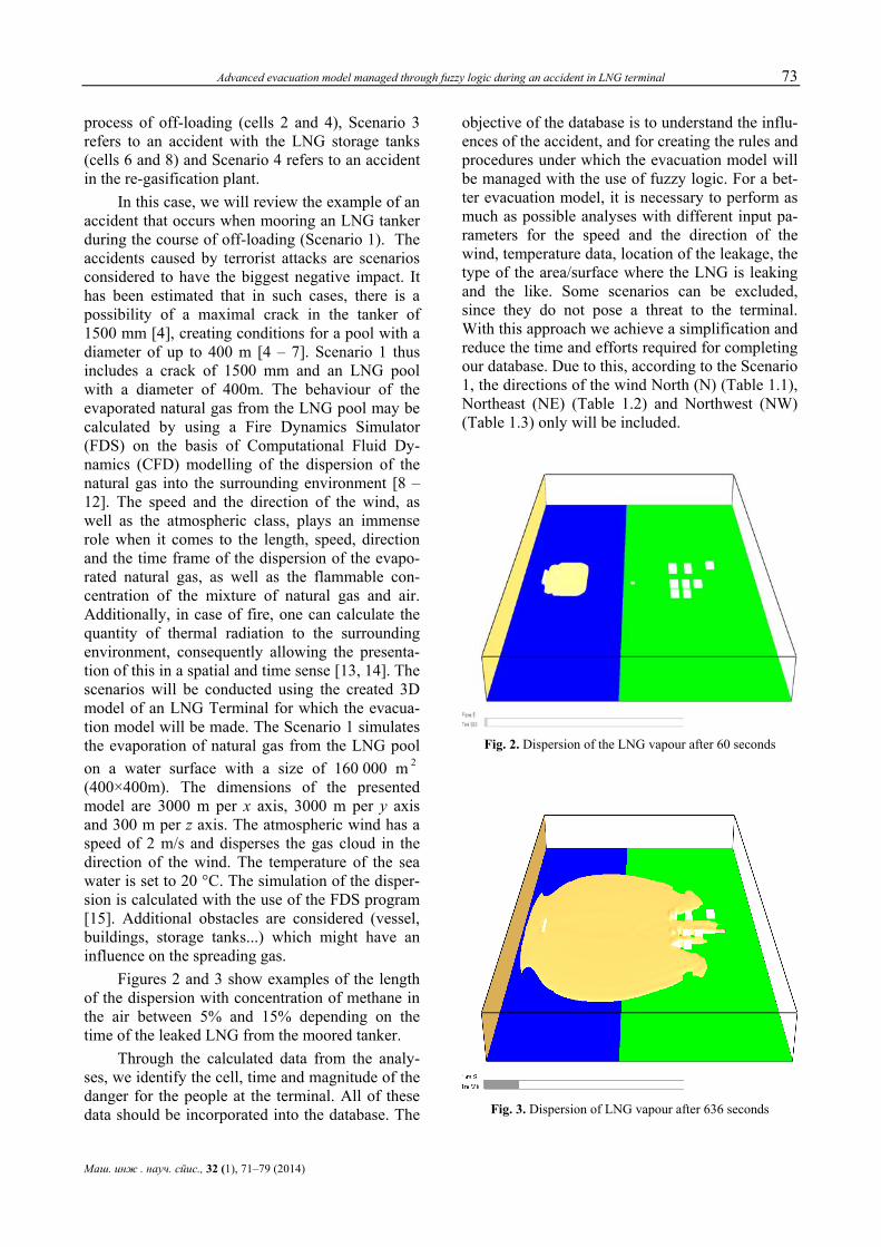
Advanced evacuation model managed through fuzzy logic during an accident in LNG terminal 73
Маш. инж . науч. спис., 32 (1), 71–79 (2014)
process of off-loading (cells 2 and 4), Scenario 3 refers to an accident with the LNG storage tanks (cells 6 and 8) and Scenario 4 refers to an accident in the re-gasification plant.
In this case, we will review the example of an accident that occurs when mooring an LNG tanker during the course of off-loading (Scenario 1). The accidents caused by terrorist attacks are scenarios considered to have the biggest negative impact. It has been estimated that in such cases, there is a possibility of a maximal crack in the tanker of 1500 mm [4], creating conditions for a pool with a diameter of up to 400 m [4 – 7]. Scenario 1 thus includes a crack of 1500 mm and an LNG pool with a diameter of 400m. The behaviour of the evaporated natural gas from the LNG pool may be calculated by using a Fire Dynamics Simulator (FDS) on the basis of Computational Fluid Dy-namics (CFD) modelling of the dispersion of the natural gas into the surrounding environment [8 – 12]. The speed and the direction of the wind, as well as the atmospheric class, plays an immense role when it comes to the length, speed, direction and the time frame of the dispersion of the evapo-rated natural gas, as well as the flammable con-centration of the mixture of natural gas and air. Additionally, in case of fire, one can calculate the quantity of thermal radiation to the surrounding environment, consequently allowing the presenta-tion of this in a spatial and time sense [13, 14]. The scenarios will be conducted using the created 3D model of an LNG Terminal for which the evacua-tion model will be made. The Scenario 1 simulates the evaporation of natural gas from the LNG pool on a water surface with a size of 160 000 m 2 (400×400m). The dimensions of the presented model are 3000 m per x axis, 3000 m per y axis and 300 m per z axis. The atmospheric wind has a speed of 2 m/s and disperses the gas cloud in the direction of the wind. The temperature of the sea water is set to 20 °C. The simulation of the disper-sion is calculated with the use of the FDS program [15]. Additional obstacles are considered (vessel, buildings, storage tanks...) which might have an influence on the spreading gas.
Figures 2 and 3 show examples of the length of the dispersion with concentration of methane in the air between 5% and 15% depending on the time of the leaked LNG from the moored tanker.
Through the calculated data from the analy-ses, we identify the cell, time and magnitude of the danger for the people at the terminal. All of these data should be incorporated into the database. The
objective of the database is to understand the influ-ences of the accident, and for creating the rules and procedures under which the evacuation model will be managed with the use of fuzzy logic. For a bet-ter evacuation model, it is necessary to perform as much as possible analyses with different input pa-rameters for the speed and the direction of the wind, temperature data, location of the leakage, the type of the area/surface where the LNG is leaking and the like. Some scenarios can be excluded, since they do not pose a threat to the terminal. With this approach we achieve a simplification and reduce the time and efforts required for completing our database. Due to this, according to the Scenario 1, the directions of the wind North (N) (Table 1.1), Northeast (NE) (Table 1.2) and Northwest (NW) (Table 1.3) only will be included.
Fig. 2. Dispersion of the LNG vapour after 60 seconds
Fig. 3. Dispersion of LNG vapour after 636 seconds
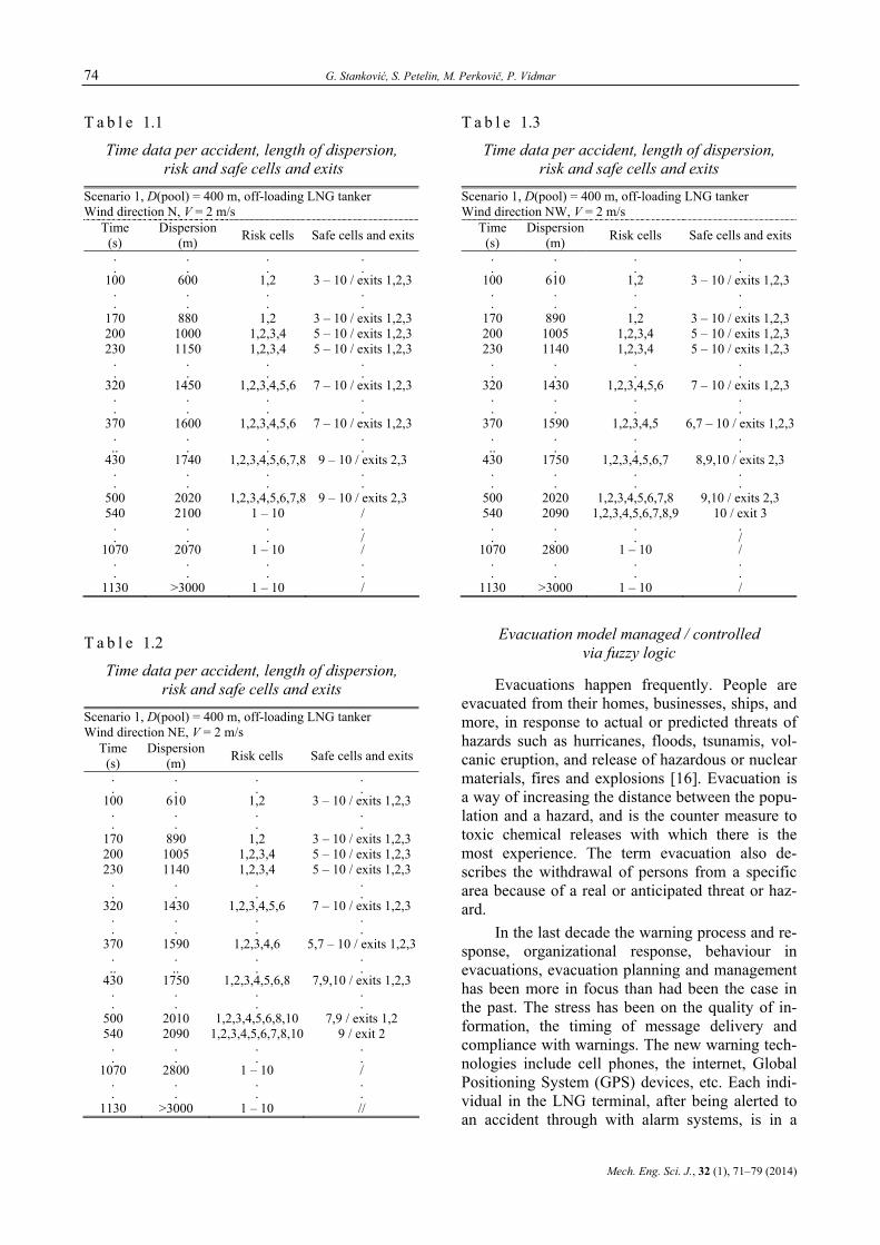
74 G. Stanković, S. Petelin, M. Perkovič, P. Vidmar
Mech. Eng. Sci. J., 32 (1), 71–79 (2014)
T a b l e 1.1
Time data per accident, length of dispersion, risk and safe cells and exits
Scenario 1, D(pool) = 400 m, off-loading LNG tanker Wind direction N, V = 2 m/s
Time (s)
Dispersion (m) Risk cells Safe cells and exits
.
. 100
.
.
.
. 600
.
.
.
. 1,2 . .
.
. 3 – 10 / exits 1,2,3
.
. 170 880 1,2 3 – 10 / exits 1,2,3 200 1000 1,2,3,4 5 – 10 / exits 1,2,3 230 1150 1,2,3,4 5 – 10 / exits 1,2,3
.
. 320
.
.
.
. 1450
.
.
.
. 1,2,3,4,5,6
.
.
.
. 7 – 10 / exits 1,2,3
.
. 370 1600 1,2,3,4,5,6 7 – 10 / exits 1,2,3
. ..
430 . .
.
. 1740
.
.
.
. 1,2,3,4,5,6,7,8
.
.
.
. 9 – 10 / exits 2,3
.
. 500 2020 1,2,3,4,5,6,7,8 9 – 10 / exits 2,3 540 2100 1 – 10 /
.
. 1070
.
.
.
. 2070
.
.
.
. 1 – 10
.
.
. / / . .
1130 >3000 1 – 10 /
T a b l e 1.2
Time data per accident, length of dispersion, risk and safe cells and exits
Scenario 1, D(pool) = 400 m, off-loading LNG tanker Wind direction NE, V = 2 m/s
Time (s)
Dispersion (m) Risk cells Safe cells and exits
.
. 100
.
.
.
. 610
.
.
.
. 1,2 . .
.
. 3 – 10 / exits 1,2,3
.
. 170 890 1,2 3 – 10 / exits 1,2,3 200 1005 1,2,3,4 5 – 10 / exits 1,2,3 230 1140 1,2,3,4 5 – 10 / exits 1,2,3
.
. 320
.
.
.
. 1430
.
.
.
. 1,2,3,4,5,6
.
.
.
. 7 – 10 / exits 1,2,3
.
. 370 1590 1,2,3,4,6 5,7 – 10 / exits 1,2,3
. ..
430 . .
. ..
1750 . .
.
. 1,2,3,4,5,6,8
.
.
.
. 7,9,10 / exits 1,2,3
.
. 500 2010 1,2,3,4,5,6,8,10 7,9 / exits 1,2 540 2090 1,2,3,4,5,6,7,8,10 9 / exit 2
.
. 1070
.
.
.
. 2800
.
.
.
. 1 – 10
.
.
.
. / . .
1130 >3000 1 – 10 //
T a b l e 1.3
Time data per accident, length of dispersion, risk and safe cells and exits
Scenario 1, D(pool) = 400 m, off-loading LNG tanker Wind direction NW, V = 2 m/s
Time (s)
Dispersion(m) Risk cells Safe cells and exits
.
. 100
.
.
.
. 610
.
.
.
. 1,2 . .
.
. 3 – 10 / exits 1,2,3
.
. 170 890 1,2 3 – 10 / exits 1,2,3 200 1005 1,2,3,4 5 – 10 / exits 1,2,3 230 1140 1,2,3,4 5 – 10 / exits 1,2,3
.
. 320
.
.
.
. 1430
.
.
.
. 1,2,3,4,5,6
.
.
.
. 7 – 10 / exits 1,2,3
.
. 370 1590 1,2,3,4,5 6,7 – 10 / exits 1,2,3
. ..
430 . .
.
. 1750
.
.
.
. 1,2,3,4,5,6,7
.
.
.
. 8,9,10 / exits 2,3
.
. 500 2020 1,2,3,4,5,6,7,8 9,10 / exits 2,3 540 2090 1,2,3,4,5,6,7,8,9 10 / exit 3
.
. 1070
.
.
.
. 2800
.
.
.
. 1 – 10
.
.
. / / . .
1130 >3000 1 – 10 /
Evacuation model managed / controlled via fuzzy logic
Evacuations happen frequently. People are evacuated from their homes, businesses, ships, and more, in response to actual or predicted threats of hazards such as hurricanes, floods, tsunamis, vol-canic eruption, and release of hazardous or nuclear materials, fires and explosions [16]. Evacuation is a way of increasing the distance between the popu-lation and a hazard, and is the counter measure to toxic chemical releases with which there is the most experience. The term evacuation also de-scribes the withdrawal of persons from a specific area because of a real or anticipated threat or haz-ard.
In the last decade the warning process and re-sponse, organizational response, behaviour in evacuations, evacuation planning and management has been more in focus than had been the case in the past. The stress has been on the quality of in-formation, the timing of message delivery and compliance with warnings. The new warning tech-nologies include cell phones, the internet, Global Positioning System (GPS) devices, etc. Each indi-vidual in the LNG terminal, after being alerted to an accident through with alarm systems, is in a
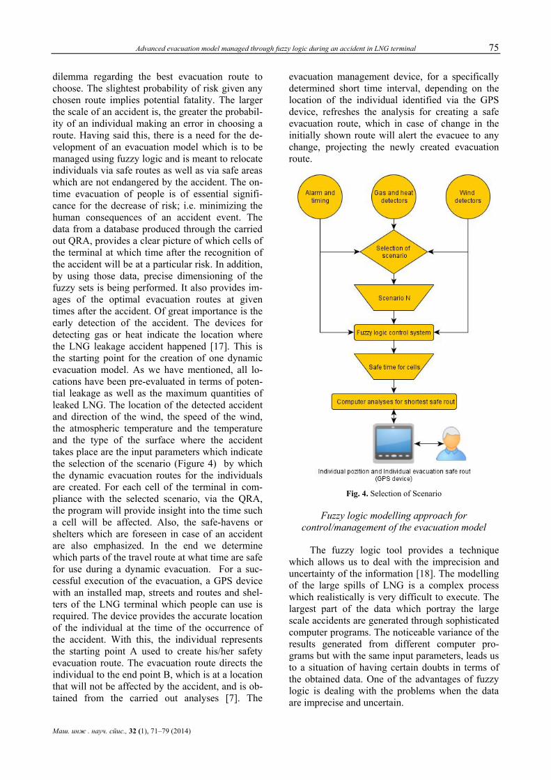
Advanced evacuation model managed through fuzzy logic during an accident in LNG terminal 75
Маш. инж . науч. спис., 32 (1), 71–79 (2014)
dilemma regarding the best evacuation route to choose. The slightest probability of risk given any chosen route implies potential fatality. The larger the scale of an accident is, the greater the probabil-ity of an individual making an error in choosing a route. Having said this, there is a need for the de-velopment of an evacuation model which is to be managed using fuzzy logic and is meant to relocate individuals via safe routes as well as via safe areas which are not endangered by the accident. The on-time evacuation of people is of essential signifi-cance for the decrease of risk; i.e. minimizing the human consequences of an accident event. The data from a database produced through the carried out QRA, provides a clear picture of which cells of the terminal at which time after the recognition of the accident will be at a particular risk. In addition, by using those data, precise dimensioning of the fuzzy sets is being performed. It also provides im-ages of the optimal evacuation routes at given times after the accident. Of great importance is the early detection of the accident. The devices for detecting gas or heat indicate the location where the LNG leakage accident happened [17]. This is the starting point for the creation of one dynamic evacuation model. As we have mentioned, all lo-cations have been pre-evaluated in terms of poten-tial leakage as well as the maximum quantities of leaked LNG. The location of the detected accident and direction of the wind, the speed of the wind, the atmospheric temperature and the temperature and the type of the surface where the accident takes place are the input parameters which indicate the selection of the scenario (Figure 4) by which the dynamic evacuation routes for the individuals are created. For each cell of the terminal in com-pliance with the selected scenario, via the QRA, the program will provide insight into the time such a cell will be affected. Also, the safe-havens or shelters which are foreseen in case of an accident are also emphasized. In the end we determine which parts of the travel route at what time are safe for use during a dynamic evacuation. For a suc-cessful execution of the evacuation, a GPS device with an installed map, streets and routes and shel-ters of the LNG terminal which people can use is required. The device provides the accurate location of the individual at the time of the occurrence of the accident. With this, the individual represents the starting point A used to create his/her safety evacuation route. The evacuation route directs the individual to the end point B, which is at a location that will not be affected by the accident, and is ob-tained from the carried out analyses [7]. The
evacuation management device, for a specifically determined short time interval, depending on the location of the individual identified via the GPS device, refreshes the analysis for creating a safe evacuation route, which in case of change in the initially shown route will alert the evacuee to any change, projecting the newly created evacuation route.
Fig. 4. Selection of Scenario
Fuzzy logic modelling approach for control/management of the evacuation model
The fuzzy logic tool provides a technique which allows us to deal with the imprecision and uncertainty of the information [18]. The modelling of the large spills of LNG is a complex process which realistically is very difficult to execute. The largest part of the data which portray the large scale accidents are generated through sophisticated computer programs. The noticeable variance of the results generated from different computer pro-grams but with the same input parameters, leads us to a situation of having certain doubts in terms of the obtained data. One of the advantages of fuzzy logic is dealing with the problems when the data are imprecise and uncertain.
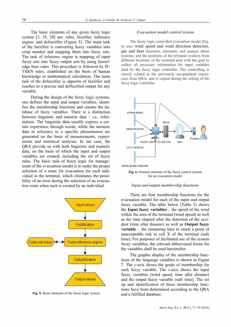
76 G. Stanković, S. Petelin, M. Perkovič, P. Vidmar
Mech. Eng. Sci. J., 32 (1), 71–79 (2014)
The basic elements of any given fuzzy logic system [3, 19, 20] are: rules, fuzzifier, inference engine, and defuzzifier (Figure 5). The main task of the fuzzifier is converting fuzzy variables into crisp number and mapping them into fuzzy sets. The task of inference engine is mapping of input fuzzy sets into fuzzy output sets by using knowl-edge base rules. This procedure is followed by IF-THEN rules, established on the basis of human knowledge or mathematical calculation. The main task of the defuzzifier is opposite of fuzzifier and reaches to a precise and deffuzified output for any variable.
During the design of the fuzzy logic systems, one defines the input and output variables, identi-fies the membership functions and creates the da-tabase of fuzzy variables. There is a distinction between linguistic and numeric data – i.e., infor-mation. The linguistic data usually express a cer-tain experience through words, while the numeric data in reference to a specific phenomenon are generated on the basis of measurements, experi-ments and statistical analyses. In our case, the QRA provide us with both linguistic and numeric data, on the basis of which the input and output variables are created, including the set of fuzzy rules. The basic task of fuzzy logic for manage-ment of the evacuation model is to make the proper selection of a route for evacuation for each indi-vidual in the terminal, which eliminates the possi-bility of an error during the selection of an evacua-tion route when such is created by an individual.
Fig. 5. Basic elements of the fuzzy logic system
Evacuation model control system
The fuzzy logic controlled evacuation model (Fig. 6) uses wind speed and wind direction detectors, gas and heat detectors, automatic and manual alarm systems, and the positions of the terminal workers from different locations of the terminal area with the goal to collect all necessary information for input variables used by the fuzzy logic controller. The controlling is closely related to the previously accumulated experi-ence from QRA, and is copied during the setting of the fuzzy logic controller.
Fig. 6. General structure of the fuzzy control system
for an evacuation model
Input and output membership functions
There are four membership functions for the evacuation model for each of the input and output fuzzy variable. The table below (Table 2) shows the Input fuzzy variables – the speed of the wind within the area of the terminal (wind speed) as well as the time elapsed after the detection of the acci-dent (time after disaster) as well as Output fuzzy variable – the remaining time to reach a point of unacceptable risk in cell X of the terminal (safe time). For purposes of facilitated use of the system fuzzy variables, the relevant abbreviated forms for the variables shall be used hereinafter.
The graphic display of the membership func-tions of the language variables is shown in Figure 7. The y-axis shows the grade of membership for each fuzzy variable. The x-axis shows the input fuzzy variables (wind speed, time after disaster) and the output fuzzy variable (safe time). The set up and identification of these membership func-tions have been determined according to the QRA and a fulfilled database.

Advanced evacuation model managed through fuzzy logic during an accident in LNG terminal 77
Маш. инж . науч. спис., 32 (1), 71–79 (2014)
T a b l e 2
Fuzzy variables and Fuzzy sets (Scenario 1: LNG pool diameter 400 m,
wind speed 2 m/s)
Linguistic variables Fuzzy set Description range
very slow (vs) 0 – 1.3
slow (s) 0.3 – 3.4
fast (f) 2.8 – 6.2
Wind speed (m/s)
very fast (vf) 5.3 – 9>
very short (vs) 0 – 55
short (s) 35 – 105
medium (m) 80 – 175
Time after disaster (s)
long (l) 140 – 250>
very short (vs) 0 – 95
short (s) 55 – 135
medium (m) 105 – 205
Safe time (s)
long (l) 265 – 280>
Fuzzy rule base and defuzzification
The rules of the FUZZY LOGIC controller are based on 'IF-THEN' conditionality. In this case wind speed and time after disaster are the factors that affect the consequence expressed as safe time. We have two variables with Fuzzy Input with four membership functions. According to this the total number of rules applied to the output fuzzy vari-able safe time is sixteen. The number of rules can also be lesser in some cases, where it is believed that some rules are not necessary or will not change anything in certain situations.
For each cell a separate matrix for fuzzy rules is being created in reference to each scenario which is part of the evacuation model. This is done with the objective that for each individual located in X cell, the fuzzy control system shall use the adequate matrix for the X cell which is intended for the scenario of the accident. As an example, Table 3 shows the matrix for fuzzy rules for evacuation Scenario l in an event when the indi-vidual is located in cell number 4.
FUZZY LOGIC controller is using the max-min composition (Mamandi). In the process of de-fuzzification, the centre of gravity of the received fuzzy set shows the output numerical value. As an example from the following chart (Fig.7) we can see the max-min composition of the 16 rules in the case where the input variables are: wind speed
2m/s, time after disaster 160 seconds. These val-ues have a grade of membership of 1. The output numerical value for safe time after the defuzzifi-cation for this case is 55 seconds.
Fig. 7. Graphical presentation of the membership functions
to the fuzzy logic controller
T a b l e 3
Matrix for fuzzy rule base for evacuation model
Safe time
Time after disaster
vs s m l
vs l m m vs
s m m s vs
f s s vs vs win
d sp
eed
vf vs vs vs vs
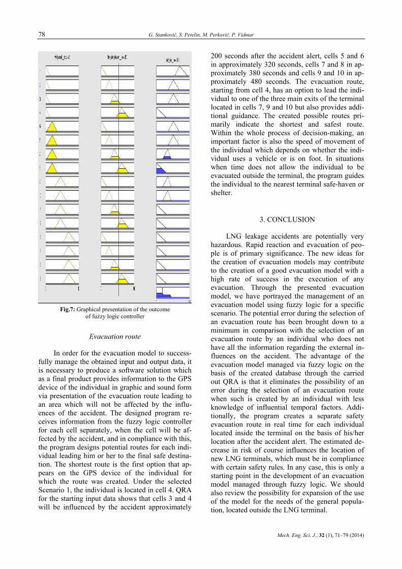
78 G. Stanković, S. Petelin, M. Perkovič, P. Vidmar
Mech. Eng. Sci. J., 32 (1), 71–79 (2014)
Fig.7: Graphical presentation of the outcome
of fuzzy logic controller
Evacuation route
In order for the evacuation model to success-fully manage the obtained input and output data, it is necessary to produce a software solution which as a final product provides information to the GPS device of the individual in graphic and sound form via presentation of the evacuation route leading to an area which will not be affected by the influ-ences of the accident. The designed program re-ceives information from the fuzzy logic controller for each cell separately, when the cell will be af-fected by the accident, and in compliance with this, the program designs potential routes for each indi-vidual leading him or her to the final safe destina-tion. The shortest route is the first option that ap-pears on the GPS device of the individual for which the route was created. Under the selected Scenario 1, the individual is located in cell 4. QRA for the starting input data shows that cells 3 and 4 will be influenced by the accident approximately
200 seconds after the accident alert, cells 5 and 6 in approximately 320 seconds, cells 7 and 8 in ap-proximately 380 seconds and cells 9 and 10 in ap-proximately 480 seconds. The evacuation route, starting from cell 4, has an option to lead the indi-vidual to one of the three main exits of the terminal located in cells 7, 9 and 10 but also provides addi-tional guidance. The created possible routes pri-marily indicate the shortest and safest route. Within the whole process of decision-making, an important factor is also the speed of movement of the individual which depends on whether the indi-vidual uses a vehicle or is on foot. In situations when time does not allow the individual to be evacuated outside the terminal, the program guides the individual to the nearest terminal safe-haven or shelter.
3. CONCLUSION
LNG leakage accidents are potentially very hazardous. Rapid reaction and evacuation of peo-ple is of primary significance. The new ideas for the creation of evacuation models may contribute to the creation of a good evacuation model with a high rate of success in the execution of any evacuation. Through the presented evacuation model, we have portrayed the management of an evacuation model using fuzzy logic for a specific scenario. The potential error during the selection of an evacuation route has been brought down to a minimum in comparison with the selection of an evacuation route by an individual who does not have all the information regarding the external in-fluences on the accident. The advantage of the evacuation model managed via fuzzy logic on the basis of the created database through the carried out QRA is that it eliminates the possibility of an error during the selection of an evacuation route when such is created by an individual with less knowledge of influential temporal factors. Addi-tionally, the program creates a separate safety evacuation route in real time for each individual located inside the terminal on the basis of his/her location after the accident alert. The estimated de-crease in risk of course influences the location of new LNG terminals, which must be in compliance with certain safety rules. In any case, this is only a starting point in the development of an evacuation model managed through fuzzy logic. We should also review the possibility for expansion of the use of the model for the needs of the general popula-tion, located outside the LNG terminal.
Advanced evacuation model managed through fuzzy logic during an accident in LNG terminal 79
Маш. инж . науч. спис., 32 (1), 71–79 (2014)
NOMENCLATURE
CFD Computational Fluid Dynamics D Pool diameter (m) FDS Fire Dynamics Simulator Fig Figure GPS Global Positioning System HAZID Hazard Identification HAZOP Hazard and Operability analysis LNG Liquid Natural Gas LOPA Layer of Protection Analysis m metre mm millimetre m2 square metre m/s metre per second N North (cardinal direction) NE Northeast (cardinal direction) NW Northwest (cardinal direction) QRA Quantitative Risk Assessment s second X number of cell x , y Cartesian coordinates 3D three-dimensional space °C degree Celsius
REFERENCES
[1] Guidance on performing risk assessment in the design of onshore LNG installations including the ship/shore inter-face, Reference number of document: OGP Draft 116901, Date: 2013-02-06.
[2] Guidelines for Chemical Process Quantitative Risk Analy-sis, Second edition, Center for Chemical Process Safety of the American Institute of Chemical Engineers, 2000.
[3] D. Teodorović, K. Vukadinović: Traffic Control and Transport Planning: A Fuzzy Sets and Neural Networks Approach, Kluwer Academic Publishers, Boston–Dord-recht–London, 1998.
[4] R M. Pitblado, J. Baik, G J. Hughes, C. Ferro, S J. Shaw: Consequences of LNG Marine Incidents. CCPS Confer-ence, Orlando, 2004.
[5] Mike Hightower, Louis Gritzo, Anay Luketa-Hanlin, John Covan, Sheldon Tieszen, Gerry Wellman, Mike Irwin, Mike Kaneshige, Brian Melof, Charles Morrow, Don Ragland: Guidance on Risk Analysis and Safety Implica-tions of a Large Liquefied Natural Gas (LNG) Spill Over Water, SANDIA REPORT, SAND2004-6258, Unlimited Release, Printed December 2004.
[6] M. Michael Hightower, Anay Luketa-Hanlin, Louis A. Gritzo, John M. Covan: Review of the Independent Risk Assessment of the Proposed Cabrillo Liquefied Natural Gas Deepwater Port Project, SANDIA REPORT, SAND2005-7339, Unlimited Release, Printed January 2006.
[7] Anay Luketa, M. Michael Hightower, Steve Attaway: Breach and Safety Analysis of Spills Over Water from Large Liquefied Natural Gas Carriers, SANDIA RE-PORT, SAND2008-3153, Unlimited Release, Printed May 2008.
[8] Yvon Mouilleau, Anousone Champassith: CFD simula-tions of the atmospheric gas dispersion using the Fire Dy-namics Simulator (FDS), Journal of Loss Prevention in the Process Industries, 22, 316–323 (2009).
[9] Filippo Gavelli, Edward Bullister, Harri Kytomaa: Appli-cation of CFD (Fluent) to LNG spills into geometrically, complex environments, Journal of Hazardous Materials, 159, 158–168 (2008).
[10] H. Oka, S. Ota: Evaluation of consequence assessment methods for pool fires on water involving large spills from liquefied natural gas carriers, J Mar Sci Technol. 13, 178–188 (2008).
[11] David W. Johnson, John B. Cornwell: Modeling the re-lease, spreading, and burning of LNG, LPG, and gasoline on water, Journal of Hazardous Materials, 140, 535–540 (2007).
[12] D. W. Hissong: Keys to modeling LNG spills on water, Journal of Hazardous Materials, 140, 465–477 (2007).
[13] Phani K. Raj: Large hydrocarbon fuel pool fires: Physical characteristics and thermal emission variations with height, Journal of Hazardous Materials, 140, 280–292 (2007).
[14] J. A. Fay: Model of spills and fires from LNG and oil tankers, Journal of Hazardous Materials, B96, 171–188 (2003).
[15] Kevin McGrattan, NIST – FDS 5 (Fire Dynamics Simu-lator).
[16] M. Liu, S. Lo, K. Yuen: A Study on Emergency Evacua-tion Planning In Case of Disasters. Proceedings of 2008 (tenth) Annual Meeting China Association for Science. Zhengzhou, China, 17–19 September 2008. CAST: China (2009).
[17] A collection of booklets describing hazards and how to manage them: Energy Fire Protection and Emergency Response, Second Edition, 2007, BP Fire Safety Series.
[18] Sanya Namee, Boonsap Witchayangkoon, Ampol Ka-roonsoontawong: Fuzzy Logic Modelling Approach for Risk Area Assessment for Hazardous Materials Trans-portation. American Transactions on Engineering & Ap-plied Sciences, 28 January 2012.
[19] Jerry M. Mendel: Fuzzy Sets for Words: A New Begin-ning, The IEEE International Conference on Fuzzy Sys-tems, 2003.
[20] S. N. Sivanandam, S. Sumathi, S. N. Deepa: Introduction to fuzzy logic using MATLAB, Springer-Verlag Berlin–Heidelberg–New York, 2007.

Mechanical Engineering – Scientific Journal, Vol. 32, No. 1, pp. 81–89 (2014) CODEN: MINSC5 – 457 In print: ISSN 1857–5293 Received: April 8, 2014 On line: ISSN 1857–9191 Accepted: May 10, 2014 UDC: 331.454:519.248]:621.645.036
Original scientific paper
THE INFLUENCE OF THE TECHNOLOGICALLY ADVANCED EVACUATION MODELS ON THE RISK ANALYSES DURING ACCIDENTS IN LNG TERMINAL
Goran Stanković, Stojan Petelin, Marko Perkovič, Peter Vidmar
Faculty for Maritime Studies and Transport, University of Ljubljana, Pot pomorščakov 4, 6320 Portorož, Republic of Slovenia
A b s t r a c t: The evacuation of people located in different safety zones of an LNG terminal is a complex prob-lem considering that the accidents involving LNG are very hazardous and post the biggest threat to the safety of the people located near the LNG leakage. The safety risk criteria define the parameters which one LNG terminal should meet in terms of safety. Those criteria also contain an evacuation as an evasive action with the objective to mitigate the influence of the LNG accident on the people at risk. Till date, not a lot of attention has been paid to tech-nologically advanced evacuations intended for LNG terminals. Creating the technologically advanced evacuation in-fluences directly on the decrease of the probability of fatalities Pf,i, thus influencing the calculation of the individual risk as well as the societal risk which results in the positioning of the F-N curve in the acceptable part of the ALARP zone. With this paper, we aim to present the difference between the safety analyses in cases when conservative data for Pf,i is being used while calculating the risk, and in cases when real data for Pf,i is been used.
Key words: evacuation model; LNG terminal; risk analysis; probability of fatality
ВЛИЈАНИЕ НА ТЕХНОЛОШКИ НАПРЕДНИ ЕВАКУАЦИОНИ МОДЕЛИ ВРЗ БЕЗБЕДНОСНИТЕ АНАЛИЗИ НА НЕЗГОДИ ВО ТЕРМИНАЛ ЗА ТЕЧЕН ПРИРОДЕН ГАС
А п с т р а к т: Евакуацијата на луѓето кои се наоѓаат во различни безбедносни зони од терминалот за течен природен гас (ТПГ) е комплексен проблем имајќи предвид дека незгодите со ТПГ се многу опасни и најголема опасност претставуваат за луѓето кои се наоѓаат блиску до истекувањето на ТПГ. Безбедносните критериуми ги дефинираат параметрите кои еден терминал за ТПГ треба да ги исполни од безбедносен аспект. Ваквите критериуми содржат и евакуација како евазивна акција со цел ублажување на влијанието од незгодата со ТПГ врз луѓето под ризик. Сè до денес недоволно внимание беше посветено на технолошки на-предни евакуации наменети за терминалите за ТПГ. Креирањето на технолошки напредна евакуација директ-но влијае врз намалување на веројатноста за смртни случаи, резултирајќи со позиционирање на кривата Ф-Н во прифатниот дел од зоната ALARP. Со овој труд сакаме да ја прикажеме разликата помеѓу безбедносните анализи во ситуација кога имаме конзервативен пристап кон определување на веројатноста за смртност при пресметувањето на ризикот, и во случај кога се користи реално определување на веројатноста од смртни случаи.
Клучни зборови: евакуационен модел; терминал за ТПГ; безбедносни анализи; веројатност од смртни случаи
1. INTRODUCTION
With the ever increasing need of energy in the world, the use of LNG is also increasing. The po-tential LNG accident with a terminal is potentially very hazardous event. The on time evacuation of people is such situations, despite the complexity of such operation, is of crucial importance and sig-
nificance. Due to this, the safety analyses include the evacuation as a factor for mitigation of the con-sequences from the accident. Vanem [1] have made analyses of accidents with LNG tankers where the risk models include evacuation and suc-cess levels of the evacuation. Tanabe and Miyake [2] have focused their research on the influences on the risk reduction concept on the basis of design
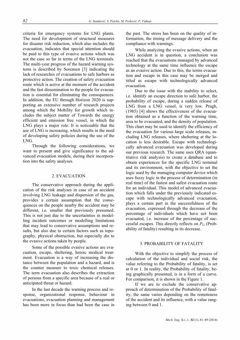
82 G. Stanković, S. Petelin, M. Perkovič, P. Vidmar
Mech. Eng. Sci. J., 32 (1), 81–89 (2014)
criteria for emergency systems for LNG plants. The need for development of structural measures for disaster risk reduction, which also includes the evacuation, indicates that special attention should be paid to this type of evasive actions which was not the case so far in terms of the LNG terminals. The multi-year progress of the hazard warning sys-tems is described by Sorensen [3] indicating the lack of researches of evacuations to safe harbors as protective action. The creation of safety evacuation route which is active at the moment of the accident and the fast dissemination to the people for evacua-tion is essential for eliminating the consequences. In addition, the EU through Horizon 2020 is sup-porting an extensive number of research projects among which the Mobility for growth which in-cludes the subject matter of Towards the energy efficient and emission free vessel, in which the LNG plays a major role. It is noticeable that the use of LNG is increasing, which results in the need of developing safety policies during the use of the LNG.
Through the following considerations, we want to present and give significance to the ad-vanced evacuation models, during their incorpora-tion into the safety analyses.
2. EVACUATION
The conservative approach during the appli-cation of the risk analyses in case of an accident involving LNG leakage and dispersion of the gas, provides a certain assumption that the conse-quences on the people nearby the accident may be different, i.e. smaller that previously presumed. This is not just due to the uncertainties in model-ling incident outcomes or modelling limitations that may lead to conservative assumptions and re-sults, but also due to certain factors such as topo-graphy, physical obstruction, but especially die to the evasive actions taken by people.
Some of the possible evasive actions are eva-cuation, escape, sheltering, heroic medical treat-ment. Evacuation is a way of increasing the dis-tance between the population and a hazard, and is the counter measure to toxic chemical releases. The term evacuation also describes the extraction of persons from a specific area because of a real or anticipated threat or hazard.
In the last decade the warning process and re-sponse, organizational response, behaviour in evacuations, evacuation planning and management has been more in focus than had been the case in
the past. The stress has been on the quality of in-formation, the timing of message delivery and the compliance with warnings.
While analyzing the evasive actions, when an LNG accident is in question, a conclusion was reached that the evacuations managed by advanced technology at the same time influence the escape as an evasive action. Due to this, the terms evacua-tion and escape in this case may be merged and titled as escape with technologically advanced evacuation.
Due to the issue with the inability to select, i.e. identify an escape direction to safe harbor, the probability of escape, during a sudden release of LNG from a LNG vessel, is very low. Prugh, (1985) [4] shows the effectiveness of the evacua-tion obtained as a function of the warning time, area to be evacuated, and the density of population. This chart may be used to identify the efficiency of the evacuation for various large scale releases, in-cluding LNG releases, where sheltering at the lo-cation is less desirable. Escape with technologi-cally advanced evacuation was developed during our previous research. The same uses QRA (quan-titative risk analysis) to create a database and to obtain experiences for the specific LNG terminal and its environment, with the objective to set the logic used by the managing computer device which uses fuzzy logic in the process of determination (in real time) of the fastest and safest evacuation route for an individual. This model of advanced evacua-tion which falls under the previously indicated es-cape with technologically advanced evacuation, plays a certain part in the successfulness of the evacuation, expressed through the decrease of the percentage of individuals which have not been evacuated, i.e. increase of the percentage of suc-cessful escapes. This directly reflects on Pf,i (Prob-ability of fatality) resulting in its decrease.
3. PROBABILITY OF FATALITY
With the objective to simplify the process of calculation of the individual and social risk, the value referring to the Probability of fatality, is set at 0 or 1. In reality, the Probability of fatality, be-ing graphically presented, is in a form of a curve. For comparison, it is shown in the Figure 1.
If we are to exclude the conservative ap-proach of determination of the Probability of fatal-ity, the same varies depending on the remoteness of the accident and its influence, with a value rang-ing between 0 and 1.
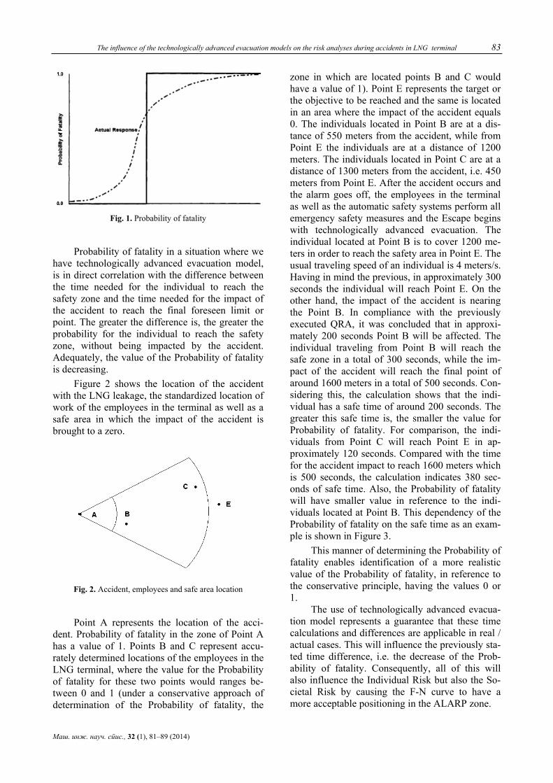
The influence of the technologically advanced evacuation models on the risk analyses during accidents in LNG terminal 83
Маш. инж. науч. спис., 32 (1), 81–89 (2014)
Fig. 1. Probability of fatality
Probability of fatality in a situation where we have technologically advanced evacuation model, is in direct correlation with the difference between the time needed for the individual to reach the safety zone and the time needed for the impact of the accident to reach the final foreseen limit or point. The greater the difference is, the greater the probability for the individual to reach the safety zone, without being impacted by the accident. Adequately, the value of the Probability of fatality is decreasing.
Figure 2 shows the location of the accident with the LNG leakage, the standardized location of work of the employees in the terminal as well as a safe area in which the impact of the accident is brought to a zero.
Fig. 2. Accident, employees and safe area location
Point A represents the location of the acci-dent. Probability of fatality in the zone of Point A has a value of 1. Points B and C represent accu-rately determined locations of the employees in the LNG terminal, where the value for the Probability of fatality for these two points would ranges be-tween 0 and 1 (under a conservative approach of determination of the Probability of fatality, the
zone in which are located points B and C would have a value of 1). Point E represents the target or the objective to be reached and the same is located in an area where the impact of the accident equals 0. The individuals located in Point B are at a dis-tance of 550 meters from the accident, while from Point E the individuals are at a distance of 1200 meters. The individuals located in Point C are at a distance of 1300 meters from the accident, i.e. 450 meters from Point E. After the accident occurs and the alarm goes off, the employees in the terminal as well as the automatic safety systems perform all emergency safety measures and the Escape begins with technologically advanced evacuation. The individual located at Point B is to cover 1200 me-ters in order to reach the safety area in Point E. The usual traveling speed of an individual is 4 meters/s. Having in mind the previous, in approximately 300 seconds the individual will reach Point E. On the other hand, the impact of the accident is nearing the Point B. In compliance with the previously executed QRA, it was concluded that in approxi-mately 200 seconds Point B will be affected. The individual traveling from Point B will reach the safe zone in a total of 300 seconds, while the im-pact of the accident will reach the final point of around 1600 meters in a total of 500 seconds. Con-sidering this, the calculation shows that the indi-vidual has a safe time of around 200 seconds. The greater this safe time is, the smaller the value for Probability of fatality. For comparison, the indi-viduals from Point C will reach Point E in ap-proximately 120 seconds. Compared with the time for the accident impact to reach 1600 meters which is 500 seconds, the calculation indicates 380 sec-onds of safe time. Also, the Probability of fatality will have smaller value in reference to the indi-viduals located at Point B. This dependency of the Probability of fatality on the safe time as an exam-ple is shown in Figure 3.
This manner of determining the Probability of fatality enables identification of a more realistic value of the Probability of fatality, in reference to the conservative principle, having the values 0 or 1.
The use of technologically advanced evacua-tion model represents a guarantee that these time calculations and differences are applicable in real / actual cases. This will influence the previously sta-ted time difference, i.e. the decrease of the Prob-ability of fatality. Consequently, all of this will also influence the Individual Risk but also the So-cietal Risk by causing the F-N curve to have a more acceptable positioning in the ALARP zone.
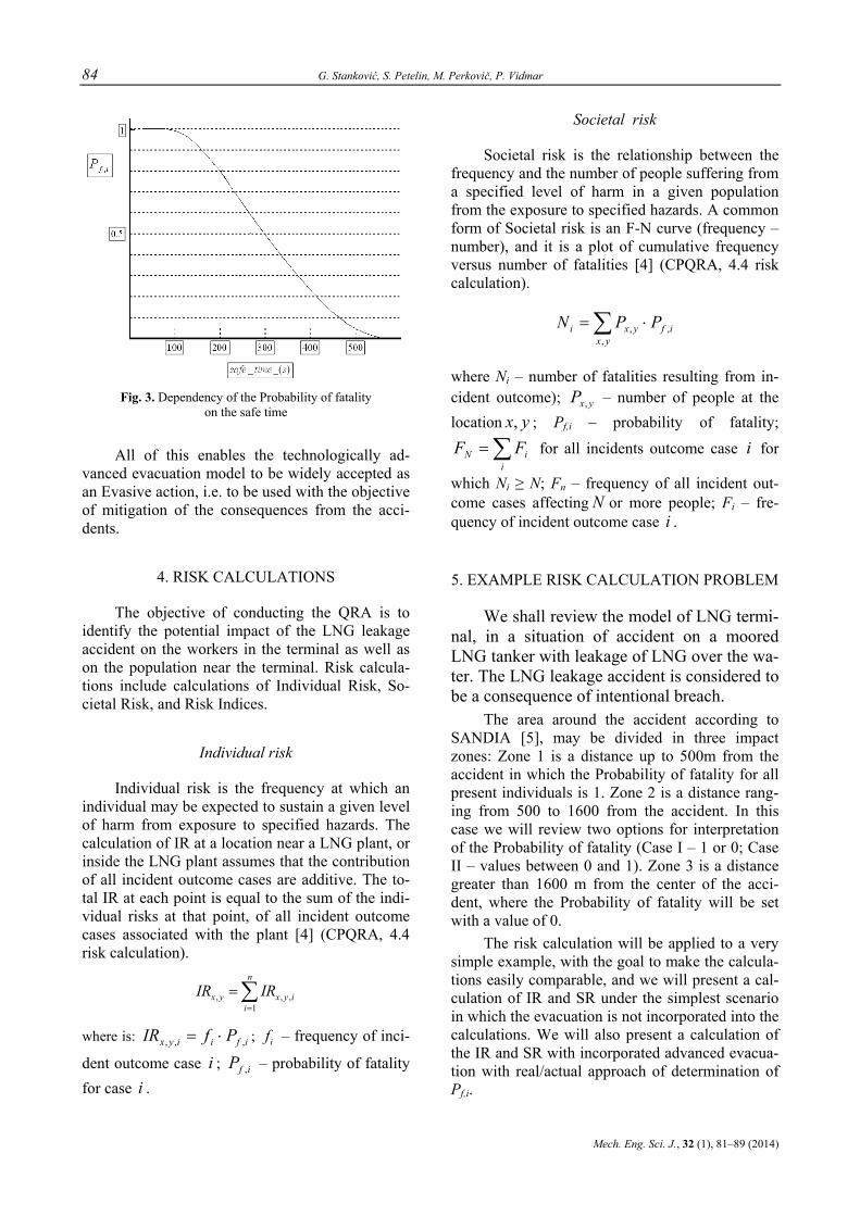
84 G. Stanković, S. Petelin, M. Perkovič, P. Vidmar
Mech. Eng. Sci. J., 32 (1), 81–89 (2014)
Fig. 3. Dependency of the Probability of fatality
on the safe time
All of this enables the technologically ad-vanced evacuation model to be widely accepted as an Evasive action, i.e. to be used with the objective of mitigation of the consequences from the acci-dents.
4. RISK CALCULATIONS
The objective of conducting the QRA is to identify the potential impact of the LNG leakage accident on the workers in the terminal as well as on the population near the terminal. Risk calcula-tions include calculations of Individual Risk, So-cietal Risk, and Risk Indices.
Individual risk
Individual risk is the frequency at which an individual may be expected to sustain a given level of harm from exposure to specified hazards. The calculation of IR at a location near a LNG plant, or inside the LNG plant assumes that the contribution of all incident outcome cases are additive. The to-tal IR at each point is equal to the sum of the indi-vidual risks at that point, of all incident outcome cases associated with the plant [4] (CPQRA, 4.4 risk calculation).
, , ,1
n
x y x y ii
IR IR=
=∑
where is: ifiiyx PfIR ,,, ⋅= ; if – frequency of inci-
dent outcome case i ; ifP , – probability of fatality for case i .
Societal risk
Societal risk is the relationship between the frequency and the number of people suffering from a specified level of harm in a given population from the exposure to specified hazards. A common form of Societal risk is an F-N curve (frequency – number), and it is a plot of cumulative frequency versus number of fatalities [4] (CPQRA, 4.4 risk calculation).
ifyx
yxi PPN ,,
, ⋅= ∑
where Ni – number of fatalities resulting from in-cident outcome); yxP , – number of people at the location yx, ; Pf,i – probability of fatality;
∑=i
iN FF for all incidents outcome case i for
which Ni ≥ N; Fn – frequency of all incident out-come cases affecting N or more people; Fi – fre-quency of incident outcome case i .
5. EXAMPLE RISK CALCULATION PROBLEM
We shall review the model of LNG termi-nal, in a situation of accident on a moored LNG tanker with leakage of LNG over the wa-ter. The LNG leakage accident is considered to be a consequence of intentional breach.
The area around the accident according to SANDIA [5], may be divided in three impact zones: Zone 1 is a distance up to 500m from the accident in which the Probability of fatality for all present individuals is 1. Zone 2 is a distance rang-ing from 500 to 1600 from the accident. In this case we will review two options for interpretation of the Probability of fatality (Case I – 1 or 0; Case II – values between 0 and 1). Zone 3 is a distance greater than 1600 m from the center of the acci-dent, where the Probability of fatality will be set with a value of 0.
The risk calculation will be applied to a very simple example, with the goal to make the calcula-tions easily comparable, and we will present a cal-culation of IR and SR under the simplest scenario in which the evacuation is not incorporated into the calculations. We will also present a calculation of the IR and SR with incorporated advanced evacua-tion with real/actual approach of determination of Pf,i.
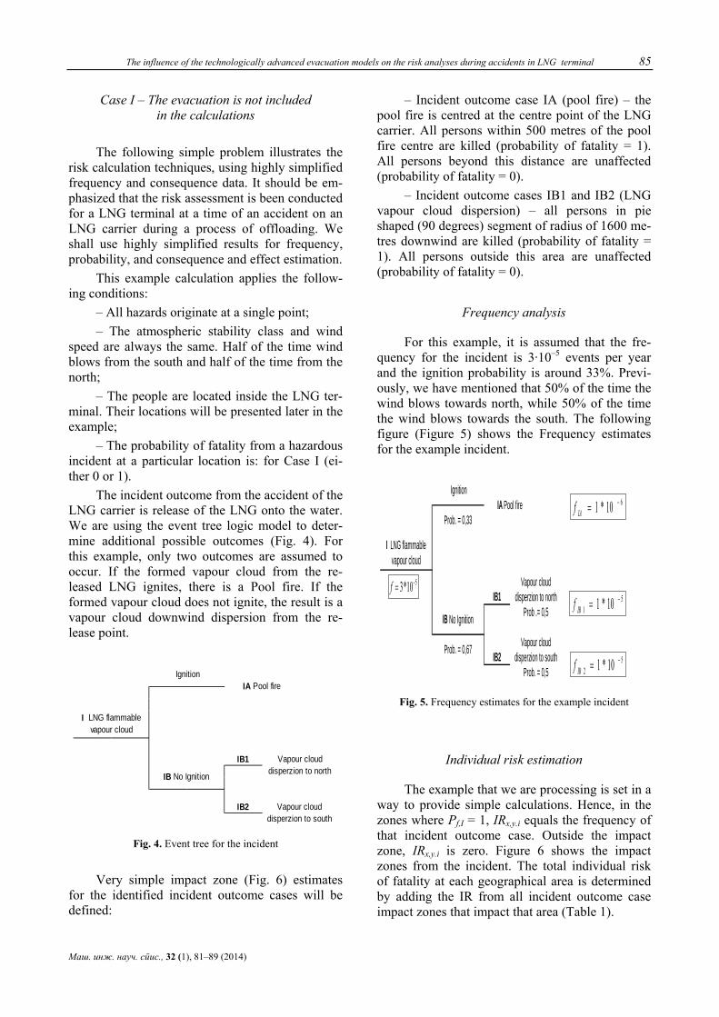
The influence of the technologically advanced evacuation models on the risk analyses during accidents in LNG terminal 85
Маш. инж. науч. спис., 32 (1), 81–89 (2014)
Case I – The evacuation is not included in the calculations
The following simple problem illustrates the risk calculation techniques, using highly simplified frequency and consequence data. It should be em-phasized that the risk assessment is been conducted for a LNG terminal at a time of an accident on an LNG carrier during a process of offloading. We shall use highly simplified results for frequency, probability, and consequence and effect estimation.
This example calculation applies the follow-ing conditions:
– All hazards originate at a single point; – The atmospheric stability class and wind
speed are always the same. Half of the time wind blows from the south and half of the time from the north;
– The people are located inside the LNG ter-minal. Their locations will be presented later in the example;
– The probability of fatality from a hazardous incident at a particular location is: for Case I (ei-ther 0 or 1).
The incident outcome from the accident of the LNG carrier is release of the LNG onto the water. We are using the event tree logic model to deter-mine additional possible outcomes (Fig. 4). For this example, only two outcomes are assumed to occur. If the formed vapour cloud from the re-leased LNG ignites, there is a Pool fire. If the formed vapour cloud does not ignite, the result is a vapour cloud downwind dispersion from the re-lease point.
IB1
I LNG flammable vapour cloud
IB No Ignition
IgnitionIA Pool fire
IB2
Vapour cloud disperzion to north
Vapour cloud disperzion to south
Fig. 4. Event tree for the incident
Very simple impact zone (Fig. 6) estimates for the identified incident outcome cases will be defined:
– Incident outcome case IA (pool fire) – the pool fire is centred at the centre point of the LNG carrier. All persons within 500 metres of the pool fire centre are killed (probability of fatality = 1). All persons beyond this distance are unaffected (probability of fatality = 0).
– Incident outcome cases IB1 and IB2 (LNG vapour cloud dispersion) – all persons in pie shaped (90 degrees) segment of radius of 1600 me-tres downwind are killed (probability of fatality = 1). All persons outside this area are unaffected (probability of fatality = 0).
Frequency analysis
For this example, it is assumed that the fre-quency for the incident is 3·10–5 events per year and the ignition probability is around 33%. Previ-ously, we have mentioned that 50% of the time the wind blows towards north, while 50% of the time the wind blows towards the south. The following figure (Figure 5) shows the Frequency estimates for the example incident.
IB1
IA Pool fire
IB2
Vapour cloud disperzion to north
Prob .= 0,5
Vapour cloud disperzion to south
Prob. = 0,5
Prob. = 0,67
I LNG flammable vapour cloud
IB No Ignition
Ignition
Prob. = 0,33
510*3 −=f
610*1 −=IAf
51 10*1 −=IBf
52 10*1 −=IBf
Fig. 5. Frequency estimates for the example incident
Individual risk estimation
The example that we are processing is set in a way to provide simple calculations. Hence, in the zones where Pf,I = 1, IRx,y.i equals the frequency of that incident outcome case. Outside the impact zone, IRx,y.i is zero. Figure 6 shows the impact zones from the incident. The total individual risk of fatality at each geographical area is determined by adding the IR from all incident outcome case impact zones that impact that area (Table 1).

86 G. Stanković, S. Petelin, M. Perkovič, P. Vidmar
Mech. Eng. Sci. J., 32 (1), 81–89 (2014)
T a b l e 1
Individual risk of fatality at each geographical area
AreaIncident
outcome case fi (per year) Pfi IRi (per year)
IA 1
IB1 1
IA 1
IB2 1
IB1 1
IB2 1
IA 1
IA 1
E
F
A
B
C
D
510*1 −
510*1 −
510*1 −
510*1 −
610*1 −
610*1 −
610*1 −
610*1 − 610*1 −
610*1 −
610*1 −
610*1 −
510*1 −
510*1 −
510*1 −
510*1 −
510*1.1 −=∑ iIR
510*1.1 −=∑ iIR
510*1 −=∑ iIR
510*1 −=∑ iIR
610*1 −=∑ iIR
610*1 −=∑ iIR
Fig. 6. Impact zones from the incident
Figure 7 shows the number and location of people in the area surrounding the LNG terminal.
The maximum IR is the highest value of IR at any geographical area.
Fig. 7. Number and location of people in the impact zones
Societal risk estimation
The first step while generating the F-H curve is to calculate the number of fatalities as a result of every incident outcome case (Tab. 2).
T a b l e 2
Estimated number of fatalities Incident outcome
caseFrequency per
yearEstimaten number
of fatalities
IA 28
IB1 50
IB2 12
610*1 −
510*1 −
510*1 −
Table 3 summarizes the cumulative frequency results. Those data are plotted to obtain the societal risk F-N curve (Fig. 8).
T a b l e 3
Cumulative frequency results Estimaten number
of fatalitiesIncident outcome
caseTotal frequency
per year
12+ IA, IB1, IB2
28+ IA, IB1
50+ IB1
>50+ none 0
510*1 −
510*1.2 −
510*1.1 −
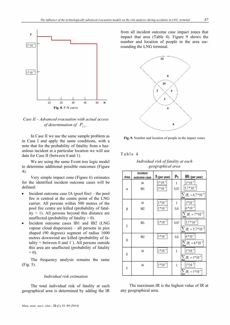
The influence of the technologically advanced evacuation models on the risk analyses during accidents in LNG terminal 87
Маш. инж. науч. спис., 32 (1), 81–89 (2014)
F
N10 20 30 40 50
510*1 −
610*1 −
Fig. 8. F-N curve
Case II – Advanced evacuation with actual access of determination of ifP , .
In Case II we use the same sample problem as in Case I and apply the same conditions, with a note that for the probability of fatality from a haz-ardous incident at a particular location we will use data for Case II (between 0 and 1).
We are using the same Event tree logic model to determine additional possible outcomes (Figure 4).
Very simple impact zone (Figure 6) estimates for the identified incident outcome cases will be defined: • Incident outcome case IA (pool fire) – the pool
fire is centred at the centre point of the LNG carrier. All persons within 500 metres of the pool fire centre are killed (probability of fatal-ity = 1). All persons beyond this distance are unaffected (probability of fatality = 0).
• Incident outcome cases IB1 and IB2 (LNG vapour cloud dispersion) – all persons in pies shaped (90 degrees) segment of radius 1600 metres downwind are killed (probability of fa-tality = between 0 and 1 ). All persons outside this area are unaffected (probability of fatality = 0).
The frequency analysis remains the same (Fig. 5).
Individual risk estimation
The total individual risk of fatality at each geographical area is determined by adding the IR
from all incident outcome case impact zones that impact that area (Table 4). Figure 9 shows the number and location of people in the area sur-rounding the LNG terminal.
Fig. 9. Number and location of people in the impact zones
T a b l e 4
Individual risk of fatality at each geographical area
AreaIncident
outcome case fi (per year) Pfi IRi (per year)
IA 1
IB1 0,57
IA 1
IB2 0,6
IB1 0,57
IB2 0,6
IA 1
IA 1
A
B
C
D
E
F
510*1 −
510*1 −
510*1 −
510*1 −
610*1 −
610*1 −
610*1 −
610*1 − 610*1 −
610*1 −
610*1 −
610*1 −
610*1 −=∑ iIR
610*1 −=∑ iIR
610*7.5 −
610*7.6 −=∑ iIR
610*6 −
610*7 −=∑ iIR610*7.5 −
610*7.5 −=∑ iIR610*6 −
610*6 −=∑ iIR
The maximum IR is the highest value of IR at
any geographical area.
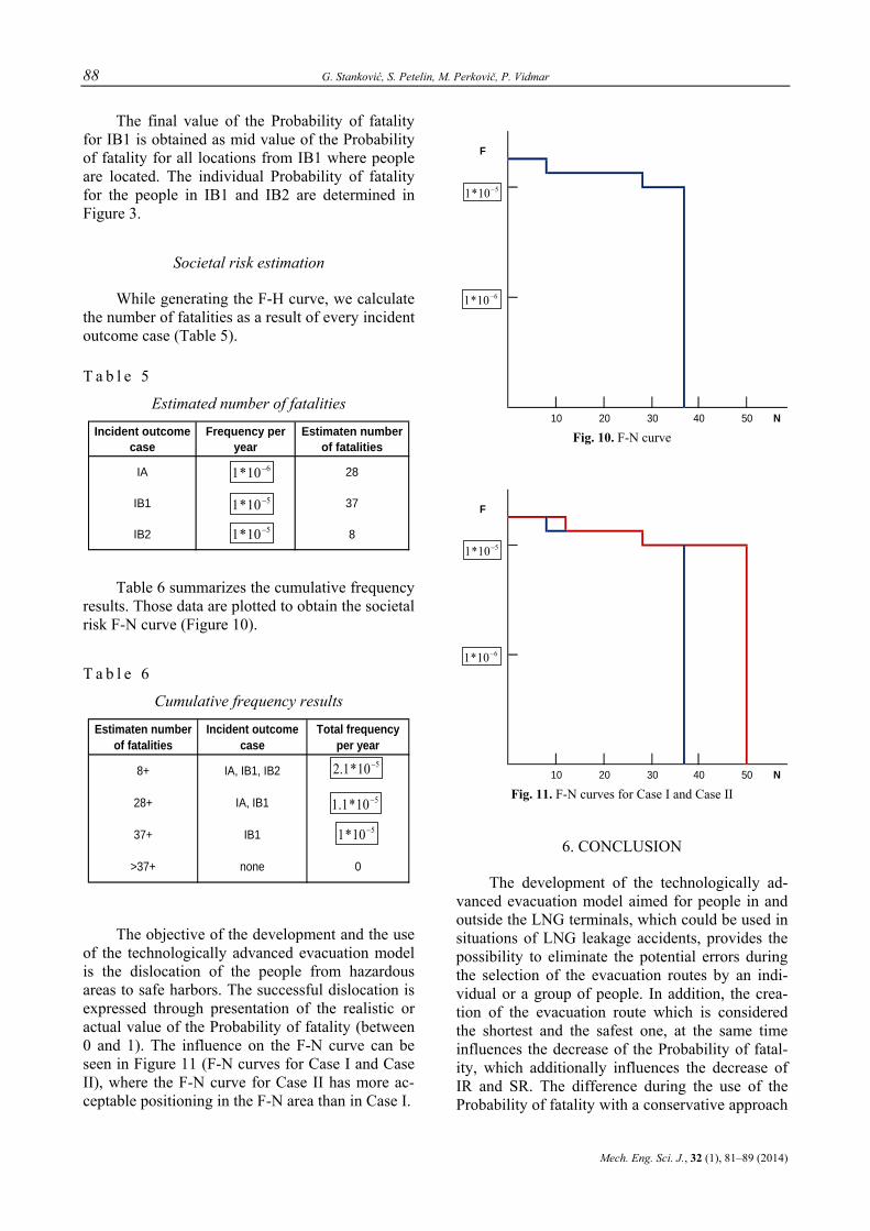
88 G. Stanković, S. Petelin, M. Perkovič, P. Vidmar
Mech. Eng. Sci. J., 32 (1), 81–89 (2014)
The final value of the Probability of fatality for IB1 is obtained as mid value of the Probability of fatality for all locations from IB1 where people are located. The individual Probability of fatality for the people in IB1 and IB2 are determined in Figure 3.
Societal risk estimation
While generating the F-H curve, we calculate the number of fatalities as a result of every incident outcome case (Table 5).
T a b l e 5
Estimated number of fatalities
Incident outcome case
Frequency per year
Estimaten number of fatalities
IA 28
IB1 37
IB2 8
610*1 −
510*1 −
510*1 −
Table 6 summarizes the cumulative frequency
results. Those data are plotted to obtain the societal risk F-N curve (Figure 10).
T a b l e 6
Cumulative frequency results
Estimaten number of fatalities
Incident outcome case
Total frequency per year
8+ IA, IB1, IB2
28+ IA, IB1
37+ IB1
>37+ none 0
510*1 −
510*1.2 −
510*1.1 −
The objective of the development and the use of the technologically advanced evacuation model is the dislocation of the people from hazardous areas to safe harbors. The successful dislocation is expressed through presentation of the realistic or actual value of the Probability of fatality (between 0 and 1). The influence on the F-N curve can be seen in Figure 11 (F-N curves for Case I and Case II), where the F-N curve for Case II has more ac-ceptable positioning in the F-N area than in Case I.
F
N10 20 30 40 50
510*1 −
610*1 −
Fig. 10. F-N curve
F
N10 20 30 40 50
510*1 −
610*1 −
Fig. 11. F-N curves for Case I and Case II
6. CONCLUSION
The development of the technologically ad-vanced evacuation model aimed for people in and outside the LNG terminals, which could be used in situations of LNG leakage accidents, provides the possibility to eliminate the potential errors during the selection of the evacuation routes by an indi-vidual or a group of people. In addition, the crea-tion of the evacuation route which is considered the shortest and the safest one, at the same time influences the decrease of the Probability of fatal-ity, which additionally influences the decrease of IR and SR. The difference during the use of the Probability of fatality with a conservative approach

The influence of the technologically advanced evacuation models on the risk analyses during accidents in LNG terminal 89
Маш. инж. науч. спис., 32 (1), 81–89 (2014)
during the determination of the value (0 or 1) and on the other hand the conservative but sufficiently realistic selection of the value for the Probability of fatality (between 0 and 1) is quite evident and we are presenting the same through a simple example. Quality developed and accurately defined techno-logically advanced evacuation model represents a guarantee for elimination of the underestimation of the value of Probability of fatality, as well as a guarantee that this approach of execution of the risk analyses will provide conservative but at the same time more realistic values.
REFERENCES
[1] Eric Vanem, A. Pedro, I. Ostvik, F. Del Castillo de Co-mas: Analysing the risk of LNG carrier operations, Reli-
ability Engineering & System Safety, 93 (9) September 2008, pp 1328–1344 (2008).
[2] Tanabe, M., Miyake, A: Risk reduction concept to provide design criteria for Emergency Systems for onshore LNG plants, Journal of Loss Prevention in the Process Indus-tries, 24, 383–390 (2011).
[3] John H. Sorensen: Hazard Warning Systems: Review of 20 Years of Progress, Natural Hazards Review, 1, 2, May, 2000.
[4] Guidelines for Chemical Process Quantitative Risk Analy-sis, Second edition, Center for chemical process safety of the American Institute of Chemical Engineers, 2000.
[5] Mike Hightower, Louis Gritzo, Anay Luketa-Hanlin, John Covan, Sheldon Tieszen, Gerry Wellman, Mike Irwin, Mike Kaneshige, Brian Melof, Charles Morrow, Don Ragland: Guidance on Risk Analysis and Safety Implica-tions of a Large Liquefied Natural Gas (LNG) Spill Over Water, SANDIA REPORT, SAND2004-6258, Unlimited Release, Printed December 2004.

Mechanical Engineering – Scientific Journal, Vol. 32, No. 1, pp. 91–98 (2014) CODEN: MINSC5 – 458 In print: ISSN 1857–5293 Received: April 26, 2014 On line: ISSN 1857–9191 Accepted: May 10, 2014 UDC: 621.436.068:[502.3:504.5)497.7)
Original scientific paper
EMISSION OF CARBON DIOXIDE FROM DIESEL ENGINES WITH EMPHASIS ON EMISSIONS IN REPUBLIC OF MACEDONIA
Dame Dimitrovski, Elena Kitanovska, Mile Dimitrovski, Done Taševski
Faculty of Mechanical Engineering, “Ss. Cyril and Methodius” University in Skopje, P.O.box 464, MK-1001 Skopje, Republic of Macedonia
A b s t r a c t: This paper presents a research work done on the arising of the air pollutants, which are a result of the combustion of fuel in diesel engines. In addition, there is a data given the increase of the consumption of diesel fuel within several consecutive years. Also there is a graphical representation of the increase of the imported used vehicles in the country, after the reduction of the customs price and excise, and then two scenarios for air pollution from these vehicles are given. In the first scenario, CO2 emissions are calculated under the current allocation of imported new and used vehicles, while in the second scenario the CO2 emissions from the imported vehicles are cal-culated, but this time 2009 was taken as the basis of the ratio of imported new and imported used vehicles, when importation of vehicles was done by the old prices of customs and excise.
Key words: diesel engine; pollution; emission; exhaust; environment; import;.transport
ЗАГАДУВАЊЕ ОД ДИЗЕЛ-МОТОРИ СО ВНАТРЕШНО СОГОРУВАЊЕ СО ОСВРТ НА ЗАГАДУВАЊЕТО ВО РЕПУБЛИКА МАКЕДОНИЈА
А п с т р а к т: Во овој труд е направено истражување на емисиите во околниот воздух кои се резултат на процесот на согорување на горивото кај дизел-моторите. Покрај тоа, дадени се податоци за зголемувањето на потрошувачката на дизел-гориво во неколку последователни години. Исто така е даден графички приказ на зголемувањето на бројот на увезени половни возила во Република Македонија по намалувањето на цари-ната и акцизата, а потоа се направени две сценарија за загадувањето на воздухот од овие возила. Во првото сценарио се пресметани емисиите на CO2 при моменталната распределба на увезени нови и увезени половни возила, додека пак во второто сценарио се пресметани емисиите на CO2 од увезените возила, но овојпат како база на односот на увезени нови и увезени половни возила е земена 2009 година, кога увозот на возила се вршеше по старите цени на царина и акциза и трендот на увезени половни возила беше значително помал.
Клучни зборови: дизел-мотор; загадување; емисии; издувни гасови; животна средина; увоз; превоз
1. INTRODUCTION
Diesel vehicles are considered as vehicles that, compared to vehicles with spark-ignition en-gine, consume less fuel to carry out the cycle, and thus less polluting. However, pollution from diesel engines is greater on local level, and this is a result from the emission of smoke and particulate matter into the atmosphere.
In Republic of Macedonia, about 30% of reg-istered passenger vehicles are with diesel engines,
and the trend continues to rise, especially in the years after the price of customs and excise on im-ported vehicles fell. After the decline of the prices on imported vehicles in 2010, a trend of buying used vehicles imported from Europe or USA in the Republic of Macedonia started with intense. How-ever, despite the dramatic increase in the number of imported used vehicles, an аnalysis of the envi-ronmental impact in the country has not been yet prepared and this situation has left room for very different expert views on this issue.
92 D. Dimitrovski, E. Kitanovska, M. Dimitrovski, D. Taševski
Mech. Eng. Sci. J., 32 (1), 91–98 (2014)
On one side, by importing used vehicles from European countries or the United States will help many people to replace their old vehicles, which are considered for great polluters of the environ-ment, with newer, thus satisfying the social aspect of residents the Republic of Macedonia. In addi-tion, this will significantly raise the average age of the vehicle fleet in the country and will influence the increase of traffic safety and the improvement of environmental quality. On the other hand, many families can now afford to purchase another vehi-cle and as a result there will be an increases the number of air pollutants in the country.
2. POLLUTION FROM DIESEL ENGINE VEHICLES
The exhaust gases from diesel engines are a mixture of gases, vapours, liquid aerosols and sub-stances composed of particles. They contain prod-ucts of combustion, which include nitrogen oxides (NO, NO2, or NOx), carbon monoxide (CO), hy-drocarbons (HC) and particulate matter (PM) re-presenting solid content in the exhaust gases, which first appears in the form of soot (combusti-ble material, usually carbon) and ash (non-combus-tible matter, mostly remnants of lubricating oil), water, sulphur oxides and polycyclic aromatic hy-drocarbons. The carbon monoxide is a compound of carbon and oxygen produced by the combustion process in the engine [1, 2].
The carbon monoxide is created when the combustion process led to partial oxidation of the carbon particles, i.e. during the process there was not enough oxygen to create carbon dioxide (СO2). It is a colourless gas, odourless and tasteless, which is poisonous to humans and animals if ex-posed to greater amounts. The amount of carbon monoxide emitted into the atmosphere from the diesel engines is very small, because they use less fuel to execute the process.
The hydrocarbons (HC) are an organic com-pound of carbon and hydrogen, that it is backward particles of fuel and lubricating oil, which are not combusted. The level of hydrocarbon particles emitted from the diesel engines is very small, es-pecially if compared with the level of hydrocarbon particles emitted from Otto engines. The amount of hydrocarbons in the exhaust gases of diesel en-gines is a result of several things: excessive or in-
sufficient mixing of fuel and air, deposits on the walls of the cylinders, fuel leaks, etc.
The nitrogen oxides (NOx) are created as a re-sult of the reaction between nitrogen and oxygen at high temperature. The formation of nitrogen oxides emissions from diesel engines occurs in poor parts of the flame, during the period of controlled com-bustion. Because of the short duration of combus-tion cycle in diesel engines, the complete combus-tion of nitrogen monoxide (NO) to nitrogen diox-ide (NO2) takes place in the atmosphere. NO2 can be found in air pollution in major urban centres, and is a highly reactive gas. High concentrations of this pollutant have sharp odour, whereas low con-centrations have a similar smell of hydrogen. NO2 is a major participant in the formation of smog [3].
The particulate matter (PM) is the biggest problem with diesel engines because of the many possible adverse effects on human health. They contain carbon particles-soot. Unlike Otto-engines, where the electric spark ignites the mixture of air and fuel, the ignition in diesel engines starts spon-taneously due to high pressure in cylinder. The mixture of air and fuel in a diesel engine is not mixed so thoroughly as in Otto engines, and there-fore "pockets" of fuel are created, and when com-busted they emit soot [4].
The diesel engines are characterized by a high presence of smoke in the exhaust, black and white. The white smoke usually occurs during cold op-eration and it is mainly composed of carbon and water vapor. On the other hand, the black smoke occurs at higher engine loads, when bigger amount of fuel is used. It allows the formation of particles of smoke, which essentially are combusted in the cylinder, but a small fraction (about 1%), are dis-charged into the atmosphere.
The amount and composition of the exhaust gases from the diesel engines depends on:
– The quality of diesel fuel used, such as chemical composition, tendency for evaporation, viscosity, ignition propensity etc. Usually when using fuels with a higher cetane number in diesel engines, there is a greater amount of smoke. This is due to the lower stability of these fuels. Therefore, it is necessary to adjust the characteristics of the fuel to the requirements of the engine;
– The type of engine, e.g. standard, turbo or injector;
– The condition of the engine or the accuracy of the system for fuel supply, condition of the cool-
Emission of carbon dioxide from diesel engines with emphasis on emissions in Republic of Macedonia 93
Маш. iнж.науч. спис., 32 (1), 91–98 (2014)
ing system etc. can significantly affect the flow of combustion and toxicity of the exhaust gases;
– The injection has a great impact on the process of combustion, and thus the effectiveness and efficiency of the engine and exhaust gas com-position. Reducing the angle of injection pump for fuel leads to a significant reduction in emissions of NOx, but also increase emissions of CH, CO and smoke, as well as increased fuel consumption;
– The composition of the mixture influence the composition and quantity of exhaust gases in diesel engines very much. If the mixture is rich than the number of zones with pronounced lack of oxygen is increased, and it results with larger amounts of CO and HC in the exhaust, and larger quantities of smoke;
– Higher air temperature gives higher tem-perature during the combustion. This affects the combustion temperature of the mixture, and the chemical reactions that contribute to faster oxida-tion of certain elements.
3. DIESEL ENGINE VEHICLES POLLUTION REDUCTION
In order to significantly reduce the amount of exhaust gases that are emitted into the atmosphere as a result of combustion in diesel engines, there are different technologies used. Because of the specificity of the cycle process development in diesel engines, or combustion in an environment with more air, emissions of CO and HC are small.
On the other hand, the challenge remains to reduce the amount of NOx, particulate matter and smoke, by making significant efforts in developing new and modern technology.
Some of the technologies used are:
Particulate filters
As the name implies, particulate filters for fil-tering solid particles from exhaust gases of diesel engines are used. They are made of ceramic ele-ments built in the shape of the hive for honey, mostly from silicon carbide.
Over time these filters are filled from the ac-cumulated particles, ash (a by-emergence from the use of oil for lubricating the engine) and exhaust gases cannot freely pass through the filter. With that comes an increase of the pressure before the filter and if pass certain limits may cause difficulty
driving the vehicle or damage to the engine. For these reasons, it is necessary that the filters are cleaned regularly and this is done by combustion or oxidation.
In the case of modern diesel engines, cutting edge technology is used, and the creation of parti-cles is reduced enough to meet the stringent re-strictions on emissions of particulate matter.
Catalysts
The catalyst is active component of the cata-lytic converter. It consists of a substrate (support-ing body) coated with precious metal catalyst. The catalytic converter substrates are usually metal or ceramic block, with thousands of tiny channels that pass through it. The channels are coated with mate-rial support, which increases their surface, thereby increasing the activity of the catalytic materials. The auxiliary material is coated with a very thin coating of finely dispersed, very small particles of precious metal, such as platinum or combinations with it.The functioning of the catalyst depends on the ratio of air - fuel mixture in the combustion. In conditions of poor mixture, i.e. poor exhaust gas, the catalyst functions as oxidizing catalyst and oxidizes the CO and the HC. However, in terms of working with a rich mixture, the catalyst primarily reduces nitrogen oxides, and then CO and HC (two-stage catalyst). Diesel engines operate with a poor mixture and because of that, the diesel cata-lyst usually operates as oxidizing catalyst. It re-duces emissions of CO and HC for more than 90% [1].
Catalyst for adsorbing the NOx
NOx adsorbing catalyst reduces the NOx from the poor flow of gas through chemical adsorption in the catalyst and subsequent disposal, in condi-tions of working with stoichiometric or rich mix-ture. The adsorption process releases CO2, which then again is re-adsorbed in the process. The ad-sorbing catalyst has a limited capacity, but it can be regenerated by transferring the flow of exhaust gas resulting from the combustion of a rich mixture into the engine.
System for selective catalytic reduction
The system for selective catalytic reduction works by chemical reduction of NO and NO2, turn-ing them into N2 and water H2O, using as reducing

94 D. Dimitrovski, E. Kitanovska, M. Dimitrovski, D. Taševski
Mech. Eng. Sci. J., 32 (1), 91–98 (2014)
agent the urea solution, which is added to the ex-haust gas. Any source of ammonia can be used, but the most common source is an aqueous solution of urea.
Recycling of exhaust gases – EGR
Recycling of exhaust gases is a technique for reducing the amount of NOx. The ERG works in a way of returning a given amount of exhaust gases back into the cylinders for combustion. In the case of diesel engines, the recycled exhaust gas replaces a certain amount of oxygen. Because NOx is pro-duced when a mixture of nitrogen and oxygen is subjected to high temperature, lower temperature in combustion chamber caused by EGR, reduces the amount of NOx in the exhaust, but at the ex-pense of some reduction of the engine perform-ance.
4. AIR POLLUTION FROM THE TRANSPORT SECTOR IN REPUBLIC OF MACEDONIA
The majority of motor fuels sold in the Re-public of Macedonia are used in the transport sec-tor, in light passenger vehicles. In the period from 2002 to 2006 in the country, more than 97% of energy consumption in the transport sector was made by passenger traffic.
The passenger traffic, that comprises passen-ger vehicles (about 88%), trucks, motorcycles, ac-counts for 92% of total generation of polluting substances emission, all of which come from the transport sector in the country, and the other mo-bile sources, that include rail, road and interna-tional air traffic, contributes with 8% of total emis-sions [5].
The problems of air pollution are more pro-nounced in urban areas. The state of traffic systems in our cities is unique because it largely does not meet fundamental principles, which are closely related to environmental modalities in modern cit-ies. In fact, such traffic systems affect the mobility of traffic connection of separate parts of the city, and with the reduction of the speed of motor vehi-cles through the city streets the motor consumes more fuel, and there are larger amounts of pollut-ing substances emitted (Fig. 1).
On the Figure 1, given below, the distribution of total emissions of pollutants from the transport sector in the Republic of Macedonia in the period
from 2001 to 2009 is shown. In the total annual emissions from all sectors nationwide, for the pe-riod 2001 to 2009 year, the largest share of the transport sector emission belongs in NOx emission (32–87%).
Fig. 1. Distribution of total emissions of pollutants
from the.transport sector
5. AIR POLLUTION FROM DIESEL ENGINES IN REPUBLIC OF MACEDONIA
According to the number of vehicles in the country, the number of spark-ignition engines is dominating, although there is a clear trend of in-creasing number of diesel engine vehicles and the number of vehicles that use a combination of gaso-line and LPG. In 2006, about 72% of the vehicles used gasoline, 24% used diesel fuel and about 4% used a combination of gasoline and LPG (Fig. 2).
Fig. 2. Distribution of passenger vehicles,
according to the fuel type
Over the years, the trend of using diesel vehi-cles in the Republic of Macedonia is increasing. On the Table 1 the distribution of passenger vehi-cles, by the fuel type in 2012, is shown.
Table 2 shows the number of registered pas-senger vehicles that use diesel fuel, depending on the type of vehicle, for the period from 2009 to 2012, and the trend of growth of the usage of die-sel vehicles.
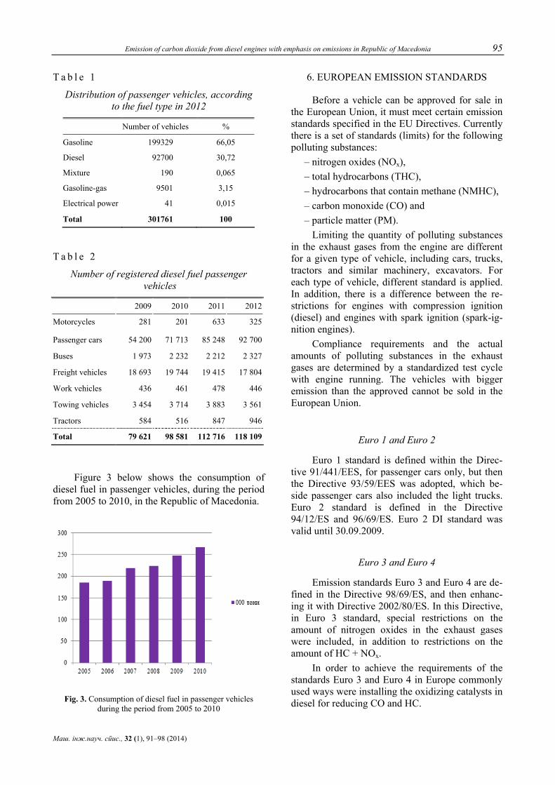
Emission of carbon dioxide from diesel engines with emphasis on emissions in Republic of Macedonia 95
Маш. iнж.науч. спис., 32 (1), 91–98 (2014)
T a b l e 1
Distribution of passenger vehicles, according to the fuel type in 2012
Number of vehicles %
Gasoline 199329 66,05
Diesel 92700 30,72
Mixture 190 0,065
Gasoline-gas 9501 3,15
Electrical power 41 0,015
Total 301761 100
T a b l e 2
Number of registered diesel fuel passenger vehicles
2009 2010 2011 2012
Motorcycles 281 201 633 325
Passenger cars 54 200 71 713 85 248 92 700
Buses 1 973 2 232 2 212 2 327
Freight vehicles 18 693 19 744 19 415 17 804
Work vehicles 436 461 478 446
Towing vehicles 3 454 3 714 3 883 3 561
Tractors 584 516 847 946
Total 79 621 98 581 112 716 118 109
Figure 3 below shows the consumption of
diesel fuel in passenger vehicles, during the period from 2005 to 2010, in the Republic of Macedonia.
Fig. 3. Consumption of diesel fuel in passenger vehicles during the period from 2005 to 2010
6. EUROPEAN EMISSION STANDARDS
Before a vehicle can be approved for sale in the European Union, it must meet certain emission standards specified in the EU Directives. Currently there is a set of standards (limits) for the following polluting substances:
– nitrogen oxides (NOx), – total hydrocarbons (THC), – hydrocarbons that contain methane (NMHC), – carbon monoxide (CO) and – particle matter (PM).
Limiting the quantity of polluting substances in the exhaust gases from the engine are different for a given type of vehicle, including cars, trucks, tractors and similar machinery, excavators. For each type of vehicle, different standard is applied. In addition, there is a difference between the re-strictions for engines with compression ignition (diesel) and engines with spark ignition (spark-ig-nition engines).
Compliance requirements and the actual amounts of polluting substances in the exhaust gases are determined by a standardized test cycle with engine running. The vehicles with bigger emission than the approved cannot be sold in the European Union.
Euro 1 and Euro 2
Euro 1 standard is defined within the Direc-tive 91/441/EES, for passenger cars only, but then the Directive 93/59/EES was adopted, which be-side passenger cars also included the light trucks. Euro 2 standard is defined in the Directive 94/12/ES and 96/69/ES. Euro 2 DI standard was valid until 30.09.2009.
Euro 3 and Euro 4
Emission standards Euro 3 and Euro 4 are de-fined in the Directive 98/69/ES, and then enhanc-ing it with Directive 2002/80/ES. In this Directive, in Euro 3 standard, special restrictions on the amount of nitrogen oxides in the exhaust gases were included, in addition to restrictions on the amount of HC + NOx.
In order to achieve the requirements of the standards Euro 3 and Euro 4 in Europe commonly used ways were installing the oxidizing catalysts in diesel for reducing CO and HC.
96 D. Dimitrovski, E. Kitanovska, M. Dimitrovski, D. Taševski
Mech. Eng. Sci. J., 32 (1), 91–98 (2014)
Euro 5 and Euro 6
For diesel engines, there are two sets of con-straints that must be implemented: Euro 5a and Euro 5b, while the Otto engines have only one - Euro 5. The implementation of Euro 5 and Euro 5a standards started in September 2009 and Euro 5b entered force in 2011.
The standard Euro 5b, for the first time, in-cludes a limit on the amount of particle number (PN). Euro 5 is improved compared to Euro 4 with more focus on the emission of particulate matter from diesel engines. Euro 5 requires installing the particle matter filters, diesel vehicles, and restricts that the emissions of particulate matter can be at most 5 mg/km.
In September 2014 the implementation of the standard Euro 6 will begin. Research of the Euro-pean Commission showed that by reducing emis-sions of nitrogen oxides, as required by Euro 6, the health conditions would improve for more than 60–90% in comparison to the Euro 5 standard. In addition, Euro 6 gives the same limit on the num-ber of particles in the exhaust as diesel and Otto engines.
In order to fulfil the Euro 5 and Euro 6 stan-dards in terms of emissions of particulate matter, all passenger cars with diesel engine must be con-structed with filter for solid particles (Tab. 3).
Republic of Macedonia, as a country not yet a member of the European Union, it is not obliged to comply with the European regulations. On the other hand, as a candidate for membership in the European Union, Republic of Macedonia has started intensive alignment and harmonization of national legislation with the legislation of the European Union. This section also included har-monization of laws, by-laws and regulations of the transport sector, and subsequently the introduction of the European emission standards for new and used vehicles.
With the purpose of meeting the limitations of the given amounts of emissions, the Directives do not require the need to use certain specific technol-ogy for reducing emissions, but the establishment and adoption of standards takes into account cur-rent technology that exists on the market.
Major technologies required to meet each stage of Euro emission limits, like improvement of the combustion air induction, riceing injection pressure and variable geometry turbocharger for air induction tailoring, showed in Table 3.
T a b l e 3
Major technologies required to meet each stage of Euro emission limits [6]
Technologies
Euro 2
• Rotary fuel pump • IDI combustion • Low pressure: 700–800 bar • ERG low pressure mechanic operation
Euro 3
• DI combustion • Injection pressure: 1300 bar • Cooled ERG • DOC for PM reduction
Euro 4
Euro 3 technology, plus: • A/F management and combustion
improvements • Electronic control of fuel injection • Injection pressure: 1600 bar • Engine tuning and mapping • 4 valves per cylinder • Electronically controlled EGR
Euro 5
Euro 4 technology, plus: • Improvement in the combustion air induction • Injection pressure: 1900 bar • Tumble and swirl • Variable geometry turbocharger • DOC+DPF • Variable valve timing • LNT may be required in some engines
Euro 6
Euro 4 technology, plus: • Injection pressure: 2100 bar • Variable geometry turbocharger for air
induction tailoring • DOC+DPF+LNT
7. IMPORT OF USED VEHICLES FROM M1 CATEGORY IN REPUBLIC OF MACEDONIA
The adoption of the Law on Amending the Law on Customs Tariff in 2010, the Republic of Macedonia lowered the excise and customs on im-ported new and used vehicles. Besides the change in the law, a new Rulebook for.single approval of a vehicle was adopted. According to the Rulebook, all imported vehicles must meet the technical re-quirements defined in it, which vary depending on the category they belong.
The Rulebook for single approval of vehicles provided a limitation of emissions depending on the category of vehicle in relation to his body shape. This paper is for vehicles in category M1, including: limo, moving vehicles, coupe, converti-ble, armorer vehicles, etc. or according to the Di-rective 95/48/ES, these are vehicles with length – 12 m, width – 2,5 m, and height – 4 m [6, 7, 8].
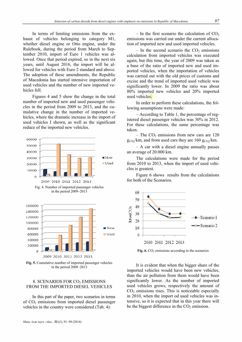
Emission of carbon dioxide from diesel engines with emphasis on emissions in Republic of Macedonia 97
Маш. iнж.науч. спис., 32 (1), 91–98 (2014)
In terms of limiting emissions from the ex-haust of vehicles belonging to category M1, whether diesel engine or Otto engine, under the Rulebook, during the period from March to Sep-tember 2010, import of Euro 1 vehicles was al-lowed. Once that period expired, so in the next six years, until August 2016, the import will be al-lowed for vehicles with Euro 2 standard and above. The adoption of these amendments, the Republic of Macedonia has started intensive importation of used vehicles and the number of new imported ve-hicles fell.
Figures 4 and 5 show the change in the total number of imported new and used passenger vehi-cles in the period from 2009 to 2013, and the cu-mulative change in the number of imported ve-hicles, where the dramatic increase in the import of used vehicles I shown, as well as the significant reduce of the imported new vehicles.
Fig. 4. Number of imported passenger vehicles
in the period 2009–2013
Fig. 5. Cumulative number of imported passenger vehicles
in the period 2009–2013
8. SCENARIOS FOR CO2 EMISSIONS FROM THE IMPORTED DIESEL VEHICLES
In this part of the paper, two scenarios in terms of CO2 emissions from imported diesel passenger vehicles in the country were considered (Tab. 4):
– In the first scenario the calculation of CO2 emissions was carried out under the current alloca-tion of imported new and used imported vehicles.
– In the second scenario the CO2 emissions calculation from imported vehicles was executed again, but this time, the year of 2009 was taken as a base of the ratio of imported new and used im-ported vehicles, when the importation of vehicles was carried out with the old prices of customs and excise and the trend of imported used vehicle was significantly lower. In 2009 the ratio was about 80% imported new vehicles and 20% imported used vehicles.
In order to perform these calculations, the fol-lowing assumptions were made:
– According to Table 1, the percentage of reg-istered diesel passenger vehicles was 30% in 2012. For these calculations, the same percentage was taken.
– The CO2 emissions from new cars are 120 gCO2/km, and from used cars they are 160 gCO2/km.
– A car with a diesel engine annually passes an average of 20.000 km.
The calculations were made for the period from 2010 to 2013, when the import of used vehi-cles is greatest.
Figure 6 shows results from the calculations for both of the Scenarios.
Fig. 6. CO2 emissions according to the scenarios
It is evident that when the bigger share of the imported vehicles would have been new vehicles, than the air pollution from them would have been significantly lower. As the number of imported used vehicles grows, respectively the amount of CO2 emissions rises. This is noticeable especially in 2010, when the import od used vehicles was in-tensive, so it is expected that in this year there will be the biggest difference in the CO2 emission.
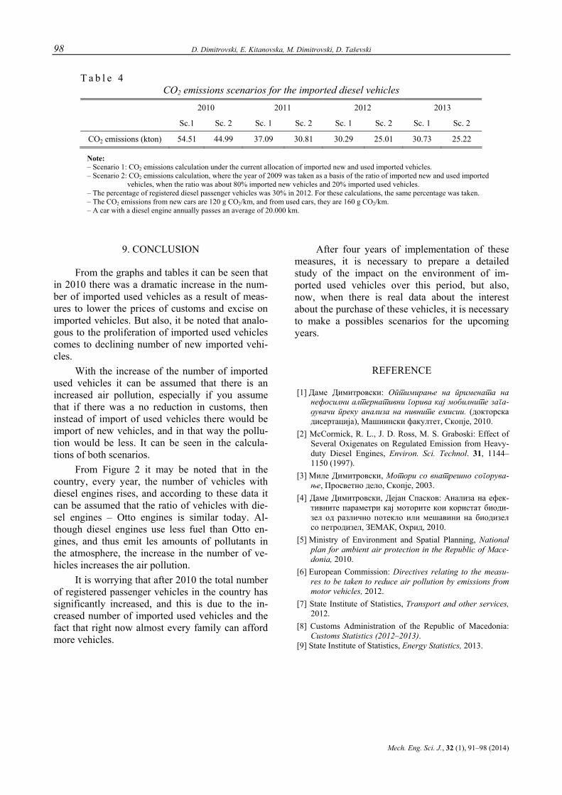
98 D. Dimitrovski, E. Kitanovska, M. Dimitrovski, D. Taševski
Mech. Eng. Sci. J., 32 (1), 91–98 (2014)
T a b l e 4 CO2 emissions scenarios for the imported diesel vehicles
2010 2011 2012 2013
Sc.1 Sc. 2 Sc. 1 Sc. 2 Sc. 1 Sc. 2 Sc. 1 Sc. 2
CO2 emissions (kton) 54.51 44.99 37.09 30.81 30.29 25.01 30.73 25.22
Note: – Scenario 1: CO2 emissions calculation under the current allocation of imported new and used imported vehicles. – Scenario 2: CO2 emissions calculation, where the year of 2009 was taken as a basis of the ratio of imported new and used imported
vehicles, when the ratio was about 80% imported new vehicles and 20% imported used vehicles. – The percentage of registered diesel passenger vehicles was 30% in 2012. For these calculations, the same percentage was taken. – The CO2 emissions from new cars are 120 g CO2/km, and from used cars, they are 160 g CO2/km. – A car with a diesel engine annually passes an average of 20.000 km.
9. CONCLUSION
From the graphs and tables it can be seen that in 2010 there was a dramatic increase in the num-ber of imported used vehicles as a result of meas-ures to lower the prices of customs and excise on imported vehicles. But also, it be noted that analo-gous to the proliferation of imported used vehicles comes to declining number of new imported vehi-cles.
With the increase of the number of imported used vehicles it can be assumed that there is an increased air pollution, especially if you assume that if there was a no reduction in customs, then instead of import of used vehicles there would be import of new vehicles, and in that way the pollu-tion would be less. It can be seen in the calcula-tions of both scenarios.
From Figure 2 it may be noted that in the country, every year, the number of vehicles with diesel engines rises, and according to these data it can be assumed that the ratio of vehicles with die-sel engines – Otto engines is similar today. Al-though diesel engines use less fuel than Otto en-gines, and thus emit les amounts of pollutants in the atmosphere, the increase in the number of ve-hicles increases the air pollution.
It is worrying that after 2010 the total number of registered passenger vehicles in the country has significantly increased, and this is due to the in-creased number of imported used vehicles and the fact that right now almost every family can afford more vehicles.
After four years of implementation of these measures, it is necessary to prepare a detailed study of the impact on the environment of im-ported used vehicles over this period, but also, now, when there is real data about the interest about the purchase of these vehicles, it is necessary to make a possibles scenarios for the upcoming years.
REFERENCE
[1] Даме Димитровски: Оптимирање на примената на нефосилни алтернативни горива кај мобилните зага-дувачи преку анализа на нивните емисии. (докторска дисертација), Машиински факултет, Скопје, 2010.
[2] McCormick, R. L., J. D. Ross, M. S. Graboski: Effect of Several Oxigenates on Regulated Emission from Heavy-duty Diesel Engines, Environ. Sci. Technol. 31, 1144–1150 (1997).
[3] Миле Димитровски, Мотори со внатрешно согорува-ње, Просветно дело, Скопје, 2003.
[4] Даме Димитровски, Дејан Спасков: Анализа на ефек-тивните параметри кај моторите кои користат биоди-зел од различно потекло или мешавини на биодизел со петродизел, ЗЕМАК, Охрид, 2010.
[5] Ministry of Environment and Spatial Planning, National plan for ambient air protection in the Republic of Mace-donia, 2010.
[6] European Commission: Directives relating to the measu-res to be taken to reduce air pollution by emissions from motor vehicles, 2012.
[7] State Institute of Statistics, Transport and other services, 2012.
[8] Customs Administration of the Republic of Macedonia: Customs Statistics (2012–2013).
[9] State Institute of Statistics, Energy Statistics, 2013.
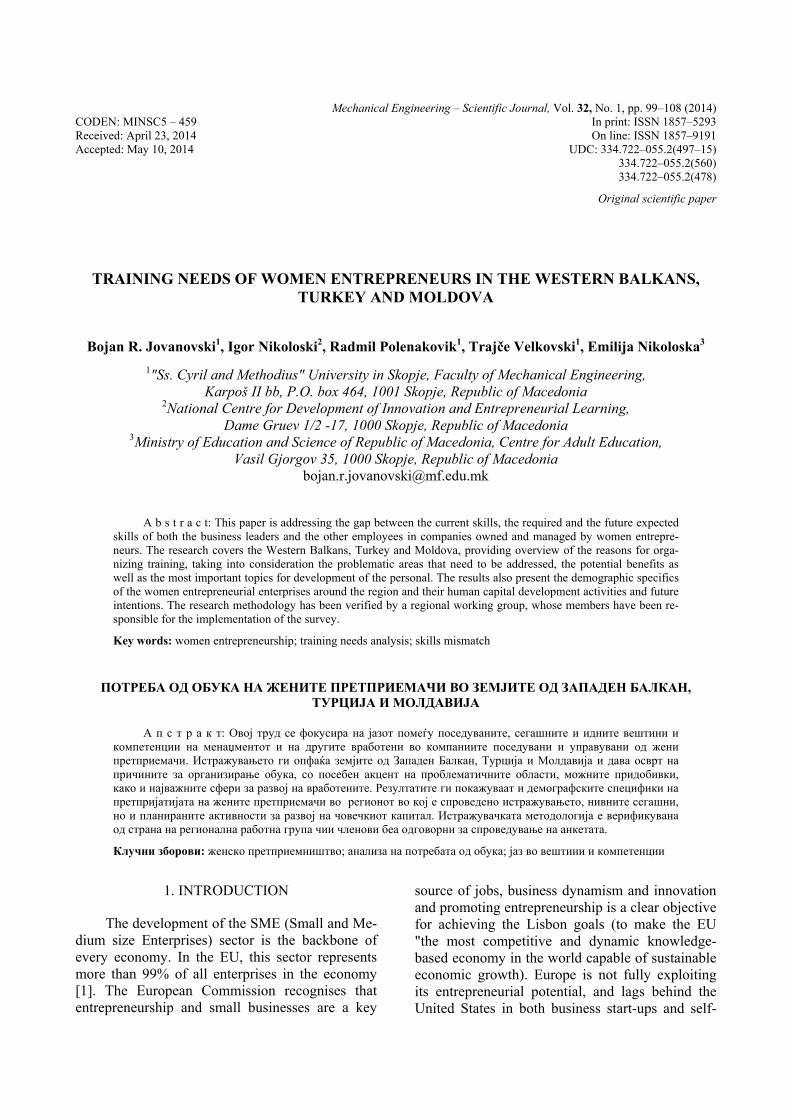
Mechanical Engineering – Scientific Journal, Vol. 32, No. 1, pp. 99–108 (2014) CODEN: MINSC5 – 459 In print: ISSN 1857–5293 Received: April 23, 2014 On line: ISSN 1857–9191 Accepted: May 10, 2014 UDC: 334.722–055.2(497–15)
334.722–055.2(560) 334.722–055.2(478)
Original scientific paper
TRAINING NEEDS OF WOMEN ENTREPRENEURS IN THE WESTERN BALKANS, TURKEY AND MOLDOVA
Bojan R. Jovanovski1, Igor Nikoloski2, Radmil Polenakovik1, Trajče Velkovski1, Emilija Nikoloska3 1"Ss. Cyril and Methodius" University in Skopje, Faculty of Mechanical Engineering,
Karpoš II bb, P.O. box 464, 1001 Skopje, Republic of Macedonia 2National Centre for Development of Innovation and Entrepreneurial Learning,
Dame Gruev 1/2 -17, 1000 Skopje, Republic of Macedonia 3Ministry of Education and Science of Republic of Macedonia, Centre for Adult Education,
Vasil Gjorgov 35, 1000 Skopje, Republic of Macedonia [email protected]
A b s t r a c t: This paper is addressing the gap between the current skills, the required and the future expected skills of both the business leaders and the other employees in companies owned and managed by women entrepre-neurs. The research covers the Western Balkans, Turkey and Moldova, providing overview of the reasons for orga-nizing training, taking into consideration the problematic areas that need to be addressed, the potential benefits as well as the most important topics for development of the personal. The results also present the demographic specifics of the women entrepreneurial enterprises around the region and their human capital development activities and future intentions. The research methodology has been verified by a regional working group, whose members have been re-sponsible for the implementation of the survey.
Key words: women entrepreneurship; training needs analysis; skills mismatch
ПОТРЕБА ОД ОБУКА НА ЖЕНИТЕ ПРЕТПРИЕМАЧИ ВО ЗЕМЈИТЕ ОД ЗАПАДЕН БАЛКАН, ТУРЦИЈА И МОЛДАВИЈА
А п с т р а к т: Овој труд се фокусира на јазот помеѓу поседуваните, сегашните и идните вештини и компетенции на менаџментот и на другите вработени во компаниите поседувани и управувани од жени претприемачи. Истражувањето ги опфаќа земјите од Западен Балкан, Турција и Молдавија и дава осврт на причините за организирање обука, со посебен акцент на проблематичните области, можните придобивки, како и најважните сфери за развој на вработените. Резултатите ги покажуваат и демографските специфики на претпријатијата на жените претприемачи во регионот во кој е спроведено истражувањето, нивните сегашни, но и планираните активности за развој на човечкиот капитал. Истражувачката методологија е верификувана од страна на регионална работна група чии членови беа одговорни за спроведување на анкетата.
Клучни зборови: женско претприемништво; анализа на потребата од обука; јаз во вештини и компетенции
1. INTRODUCTION
The development of the SME (Small and Me-dium size Enterprises) sector is the backbone of every economy. In the EU, this sector represents more than 99% of all enterprises in the economy [1]. The European Commission recognises that entrepreneurship and small businesses are a key
source of jobs, business dynamism and innovation and promoting entrepreneurship is a clear objective for achieving the Lisbon goals (to make the EU "the most competitive and dynamic knowledge-based economy in the world capable of sustainable economic growth). Europe is not fully exploiting its entrepreneurial potential, and lags behind the United States in both business start-ups and self-
100 B. R. Jovanovski, I. Nikoloski, R. Polenakovik, T. Velkovski, E. Nikoloska
Mech. Eng. Sci. J., 32 (1), 99–108 (2014)
employment. Women entrepreneurship is also im-portant to the EU for both gender equality and economic growth. ”In terms of policy recommen-dations, stakeholders underline the importance of better data on which to base policies, as well as the reinforcement of support structures for female en-trepreneurs such as the provision of information and training, business networks, business support services, and facilitating access to both human and financial capital for women” [2]. The Global En-trepreneurship Monitor has shown that an average entrepreneur is double more likely to be male than female [3], which indicates that it is necessary to address the women entrepreneurs as a specific tar-get group in order to provide custom made support for starting and growing of their businesses.
According to the study undertaken by the European Commission in 2008 on women innova-tors and entrepreneurs [4], there were identified: three types of women's obstacles to innovative en-trepreneurship:
1. Contextual obstacles: educational choices, traditional views and stereotypes about women, science and innovation;
2. Economic obstacles: innovation sector re-quiring substantial investment and women being seen less credible financially than men;
3. Soft obstacles: lack of access to technical scientific and general business networks, lack of business training, role models and entrepreneurship skills.
Based on this, the group soft obstacles play an important role in lacking the women to foster and expand businesses. Due to this, according to the EU Small Business Act for Europe 10, the skills mismatch is going to stay very high in the EU agenda, which was confirmed with the EU 2020 Strategy documents. By renewed emphasis by cur-rent European Commission policies for a more en-trepreneurial Europe and for women entrepreneur-ship as a priority pillar within the SBA (Small Business Act), ensuring policy alignment, monito-ring systems and support frameworks for women's entrepreneurship requires a concerted commitment by all pre-accession countries to bring forward and ensure improvements in women's employment and participation in the economy.
Training is a fundamental element in fostering the competitiveness of women entrepreneurs and an instrument that support companies growth and development. The system analyses of the training needs are essential in order to design the training in such manner that can be tailored specifically to
existing enterprises’ needs. This eliminates provi-sion of training which is overabundant and in-creases provision of training which is lacking - which results in greater system efficiency.
2. RESEARCH METHODOLOGY
In order to conduct effective research, the im-plementing team has designed the following re-search methodology:
Phase I: Establishment of a regional working group
Working group composed on 9 participants from relevant institutions from the researched countries was established. The working group’s main objectives were verification of the methodol-ogy, adaptation of the questionnaire and conduct-ing the survey.
Phase II: Analysis of TNA good practice methodologies
The implementation team have analyzed the good practice methodologies for national and re-gional training needs analysis methodologies. The scope of the analysis has also included women en-trepreneurship specific aspects, as well as regional aspects and good practices.
Phase III: Development of the methodology and the survey questionnaire
Based on the analysis, the implementation team have developed the TNA methodology and questionnaire. The finalization of these documents was verified with the working group including country specific aspects, as well as business sector interest into the methodology.
Phase IV: Data collection process The survey was conducted through online
data collection system, translated into all of the countries’ languages. Each working group member in cooperation with women business support or-ganizations in their respective country promoted and supervised the implementation of the survey process. After the finalization of this process, 1856 successfully filled in questionnaires from 9 coun-tries were uploaded on the on-line data base.
Phase V: Preparation of country report Each working group member has prepared
country specific report. The reports presented the background information for women entrepreneur-
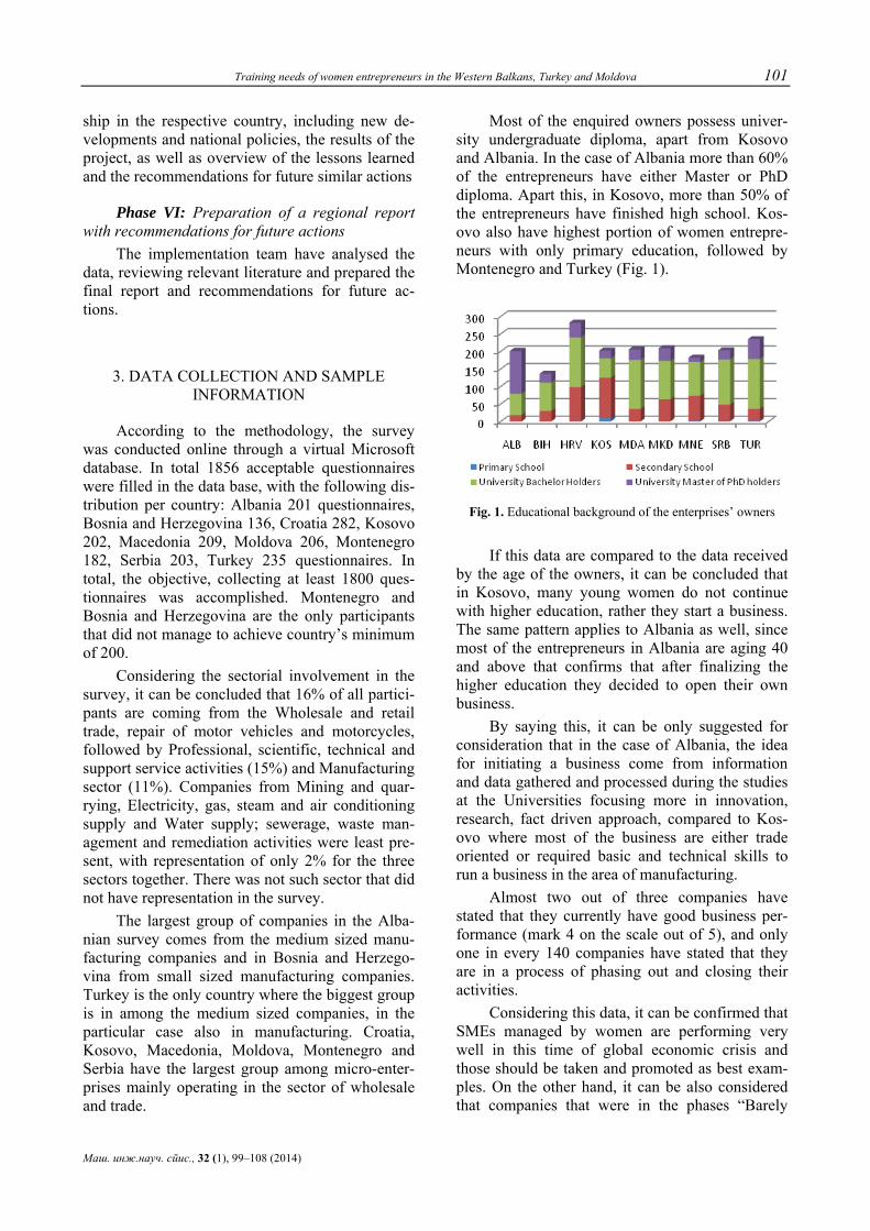
Training needs of women entrepreneurs in the Western Balkans, Turkey and Moldova 101
Маш. инж.науч. спис., 32 (1), 99–108 (2014)
ship in the respective country, including new de-velopments and national policies, the results of the project, as well as overview of the lessons learned and the recommendations for future similar actions
Phase VI: Preparation of a regional report with recommendations for future actions
The implementation team have analysed the data, reviewing relevant literature and prepared the final report and recommendations for future ac-tions.
3. DATA COLLECTION AND SAMPLE INFORMATION
According to the methodology, the survey was conducted online through a virtual Microsoft database. In total 1856 acceptable questionnaires were filled in the data base, with the following dis-tribution per country: Albania 201 questionnaires, Bosnia and Herzegovina 136, Croatia 282, Kosovo 202, Macedonia 209, Moldova 206, Montenegro 182, Serbia 203, Turkey 235 questionnaires. In total, the objective, collecting at least 1800 ques-tionnaires was accomplished. Montenegro and Bosnia and Herzegovina are the only participants that did not manage to achieve country’s minimum of 200.
Considering the sectorial involvement in the survey, it can be concluded that 16% of all partici-pants are coming from the Wholesale and retail trade, repair of motor vehicles and motorcycles, followed by Professional, scientific, technical and support service activities (15%) and Manufacturing sector (11%). Companies from Mining and quar-rying, Electricity, gas, steam and air conditioning supply and Water supply; sewerage, waste man-agement and remediation activities were least pre-sent, with representation of only 2% for the three sectors together. There was not such sector that did not have representation in the survey.
The largest group of companies in the Alba-nian survey comes from the medium sized manu-facturing companies and in Bosnia and Herzego-vina from small sized manufacturing companies. Turkey is the only country where the biggest group is in among the medium sized companies, in the particular case also in manufacturing. Croatia, Kosovo, Macedonia, Moldova, Montenegro and Serbia have the largest group among micro-enter-prises mainly operating in the sector of wholesale and trade.
Most of the enquired owners possess univer-sity undergraduate diploma, apart from Kosovo and Albania. In the case of Albania more than 60% of the entrepreneurs have either Master or PhD diploma. Apart this, in Kosovo, more than 50% of the entrepreneurs have finished high school. Kos-ovo also have highest portion of women entrepre-neurs with only primary education, followed by Montenegro and Turkey (Fig. 1).
Fig. 1. Educational background of the enterprises’ owners
If this data are compared to the data received by the age of the owners, it can be concluded that in Kosovo, many young women do not continue with higher education, rather they start a business. The same pattern applies to Albania as well, since most of the entrepreneurs in Albania are aging 40 and above that confirms that after finalizing the higher education they decided to open their own business.
By saying this, it can be only suggested for consideration that in the case of Albania, the idea for initiating a business come from information and data gathered and processed during the studies at the Universities focusing more in innovation, research, fact driven approach, compared to Kos-ovo where most of the business are either trade oriented or required basic and technical skills to run a business in the area of manufacturing.
Almost two out of three companies have stated that they currently have good business per-formance (mark 4 on the scale out of 5), and only one in every 140 companies have stated that they are in a process of phasing out and closing their activities.
Considering this data, it can be confirmed that SMEs managed by women are performing very well in this time of global economic crisis and those should be taken and promoted as best exam-ples. On the other hand, it can be also considered that companies that were in the phases “Barely
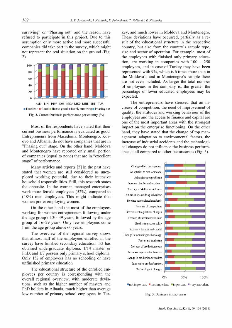
102 B. R. Jovanovski, I. Nikoloski, R. Polenakovik, T. Velkovski, E. Nikoloska
Mech. Eng. Sci. J., 32 (1), 99–108 (2014)
surviving” or “Phasing out” and the reason have refused to participate in this project. Due to this assumption only more active and more successful companies did take part in the survey, which might not represent the real situation on the ground (Fig. 2).
Fig. 2. Current business performance per country (%)
Most of the respondents have stated that their current business performance is evaluated as good. Entrepreneurs from Macedonia, Montenegro, Kos-ovo and Albania, do not have companies that are in ”Phasing out” stage. On the other hand, Moldova and Montenegro have reported only small portion of companies (equal to none) that are in “excellent stage” of performance.
Many articles and reports [5] in the past have stated that women are still considered as unex-plored working potential, due to their intensive household responsibilities. Still, this research states the opposite. In the women managed enterprises work more female employees (52%), compared to (48%) men employees. This might indicate that women prefer employing women.
On the other hand the most of the employees working for women entrepreneurs following under the age group of 30–39 years, followed by the age group of 16–29 years. Only few employees come from the age group above 60 years.
The overview of the regional survey shows that almost half of the employees enrolled in the survey have finished secondary education, 1/3 has obtained undergraduate diploma, 1/14 master or PhD, and 1/7 possess only primary school diploma. Only 1% of employees has no schooling or have unfinished primary education
The educational structure of the enrolled em-ployees per country is corresponding with the overall regional overview, with moderate devia-tions, such as the higher number of masters and PhD holders in Albania, much higher than average low number of primary school employees in Tur-
key, and much lower in Moldova and Montenegro. These deviations have occurred, partially as a re-sult of the educational structure in the respective country, but also from the country’s sample type, size and sector of operation. For example, most of the employees with finished only primary educa-tion, are working in companies with 100 – 250 employees, and in case of Turkey they have been represented with 9%, which is 6 times more than in the Moldova’s and in Montenegro’s sample there are not even included. As larger the total number of employees in the company is, the greater the percentage of lower educated employees may be expected.
The entrepreneurs have stressed that an in-crease of competition, the need of improvement of quality, the attitudes and working behaviour of the employees and the access to finance and capital are one of the most important areas with the strongest impact on the enterprise functioning. On the other hand, they have stated that the change of top man-agement, adaptation to environmental factors, the increase of industrial accidents and the technologi-cal changes do not influence the business perform-ance at all compared to other factors/areas (Fig. 3).
Fig. 3. Business impact areas
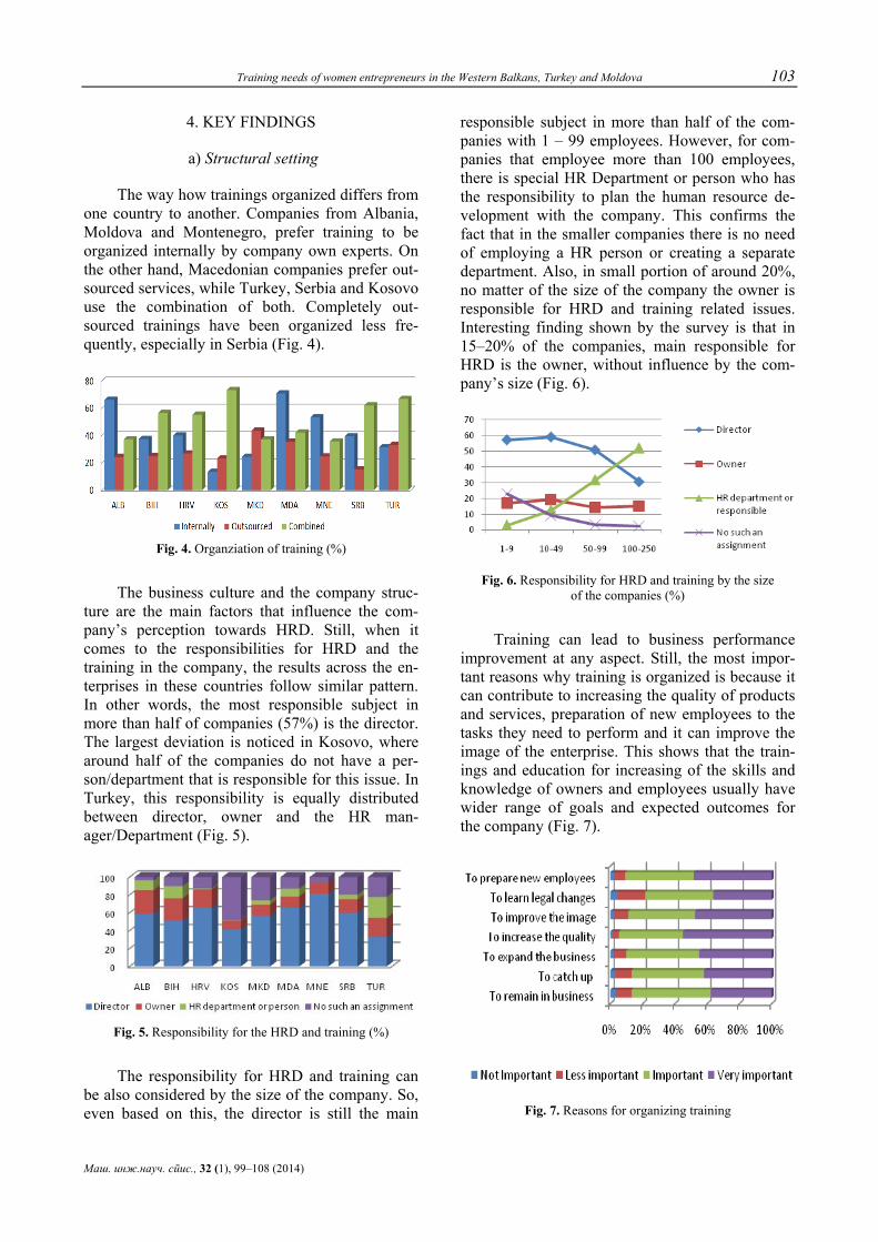
Training needs of women entrepreneurs in the Western Balkans, Turkey and Moldova 103
Маш. инж.науч. спис., 32 (1), 99–108 (2014)
4. KEY FINDINGS
а) Structural setting
The way how trainings organized differs from one country to another. Companies from Albania, Moldova and Montenegro, prefer training to be organized internally by company own experts. On the other hand, Macedonian companies prefer out-sourced services, while Turkey, Serbia and Kosovo use the combination of both. Completely out-sourced trainings have been organized less fre-quently, especially in Serbia (Fig. 4).
Fig. 4. Organziation of training (%)
The business culture and the company struc-ture are the main factors that influence the com-pany’s perception towards HRD. Still, when it comes to the responsibilities for HRD and the training in the company, the results across the en-terprises in these countries follow similar pattern. In other words, the most responsible subject in more than half of companies (57%) is the director. The largest deviation is noticed in Kosovo, where around half of the companies do not have a per-son/department that is responsible for this issue. In Turkey, this responsibility is equally distributed between director, owner and the HR man-ager/Department (Fig. 5).
Fig. 5. Responsibility for the HRD and training (%)
The responsibility for HRD and training can be also considered by the size of the company. So, even based on this, the director is still the main
responsible subject in more than half of the com-panies with 1 – 99 employees. However, for com-panies that employee more than 100 employees, there is special HR Department or person who has the responsibility to plan the human resource de-velopment with the company. This confirms the fact that in the smaller companies there is no need of employing a HR person or creating a separate department. Also, in small portion of around 20%, no matter of the size of the company the owner is responsible for HRD and training related issues. Interesting finding shown by the survey is that in 15–20% of the companies, main responsible for HRD is the owner, without influence by the com-pany’s size (Fig. 6).
Fig. 6. Responsibility for HRD and training by the size of the companies (%)
Training can lead to business performance improvement at any aspect. Still, the most impor-tant reasons why training is organized is because it can contribute to increasing the quality of products and services, preparation of new employees to the tasks they need to perform and it can improve the image of the enterprise. This shows that the train-ings and education for increasing of the skills and knowledge of owners and employees usually have wider range of goals and expected outcomes for the company (Fig. 7).
Fig. 7. Reasons for organizing training
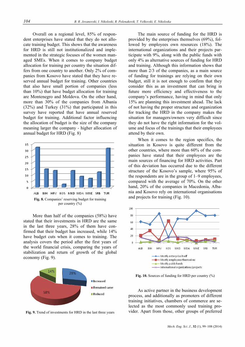
104 B. R. Jovanovski, I. Nikoloski, R. Polenakovik, T. Velkovski, E. Nikoloska
Mech. Eng. Sci. J., 32 (1), 99–108 (2014)
Overall on a regional level, 85% of respon-dent enterprises have stated that they do not allo-cate training budget. This shows that the awareness for HRD is still not institutionalized and imple-mented in the strategic focuses of the women man-aged SMEs. When it comes to company budget allocation for training per country the situation dif-fers from one country to another. Only 2% of com-panies from Kosovo have stated that they have re-served annual budget for training. Other countries that also have small portion of companies (less than 10%) that have budget allocation for training are Montenegro and Moldova. On the other hand, more than 30% of the companies from Albania (32%) and Turkey (31%) that participated in this survey have reported that have annual reserved budget for training. Additional factor influencing the allocation of budget is the size of the company meaning larger the company - higher allocation of annual budget for HRD (Fig. 8)
Fig. 8. Companies’ reserving budget for training
per country (%)
More than half of the companies (58%) have stated that their investments in HRD are the same in the last three years, 28% of them have con-firmed that their budget has increased, while 14% have budget cuts when it comes to training. The analysis covers the period after the first years of the world financial crisis, comparing the years of stabilization and return of growth of the global economy (Fig. 9).
Fig. 9. Trend of investments for HRD in the last three years
The main source of funding for the HRD is provided by the enterprises themselves (69%), fol-lowed by employees own resources (18%). The international organizations and their projects par-ticipate with 9%, along with the public funds with only 4% as alternative sources of funding for HRD and training. Although this information shows that more than 2/3 of the companies, as a main source of funding for trainings are relying on their own budget, still it is not enough to confirm that they consider this as an investment that can bring in future more efficiency and effectiveness to the company’s performance, having in mind that only 15% are planning this investment ahead. The lack of not having the proper structure and organization for tracking the HRD in the company makes the situation for managers/owners very difficult since they do not have the right information for the vol-ume and focus of the trainings that their employees attend by their own.
When it comes to the region specifics, the situation in Kosovo is quite different from the other countries, where more than 60% of the com-panies have stated that their employees are the main sources of financing for HRD activities. Part of this deviation has occurred due to the different structure of the Kosovo’s sample, where 95% of the respondents are in the group of 1–9 employees, compared with the average of 70%. On the other hand, 20% of the companies in Macedonia, Alba-nia and Kosovo rely on international organisations and projects for training (Fig. 10).
Fig. 10. Sources of funding for HRD per country (%)
As active partner in the business development process, and additionally as promoters of different training initiatives, chambers of commerce are se-lected as the most commonly used training pro-vider. Apart from those, other groups of preferred
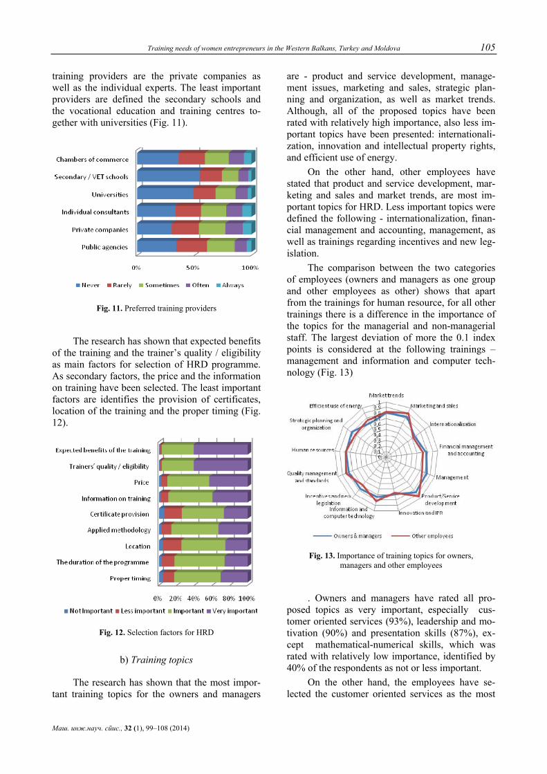
Training needs of women entrepreneurs in the Western Balkans, Turkey and Moldova 105
Маш. инж.науч. спис., 32 (1), 99–108 (2014)
training providers are the private companies as well as the individual experts. The least important providers are defined the secondary schools and the vocational education and training centres to-gether with universities (Fig. 11).
Fig. 11. Preferred training providers
The research has shown that expected benefits of the training and the trainer’s quality / eligibility as main factors for selection of HRD programme. As secondary factors, the price and the information on training have been selected. The least important factors are identifies the provision of certificates, location of the training and the proper timing (Fig. 12).
Fig. 12. Selection factors for HRD
b) Training topics
The research has shown that the most impor-tant training topics for the owners and managers
are - product and service development, manage-ment issues, marketing and sales, strategic plan-ning and organization, as well as market trends. Although, all of the proposed topics have been rated with relatively high importance, also less im-portant topics have been presented: internationali-zation, innovation and intellectual property rights, and efficient use of energy.
On the other hand, other employees have stated that product and service development, mar-keting and sales and market trends, are most im-portant topics for HRD. Less important topics were defined the following - internationalization, finan-cial management and accounting, management, as well as trainings regarding incentives and new leg-islation.
The comparison between the two categories of employees (owners and managers as one group and other employees as other) shows that apart from the trainings for human resource, for all other trainings there is a difference in the importance of the topics for the managerial and non-managerial staff. The largest deviation of more the 0.1 index points is considered at the following trainings – management and information and computer tech-nology (Fig. 13)
Fig. 13. Importance of training topics for owners, managers and other employees
. Owners and managers have rated all pro-posed topics as very important, especially cus-tomer oriented services (93%), leadership and mo-tivation (90%) and presentation skills (87%), ex-cept mathematical-numerical skills, which was rated with relatively low importance, identified by 40% of the respondents as not or less important.
On the other hand, the employees have se-lected the customer oriented services as the most

106 B. R. Jovanovski, I. Nikoloski, R. Polenakovik, T. Velkovski, E. Nikoloska
Mech. Eng. Sci. J., 32 (1), 99–108 (2014)
important for business development. But according the EU legislation and directives and mathemati-cal-numerical skills, finance, accounting and con-trolling, as well as organization and management, have been rated as the least important topics.
The surveyed companies’ representatives, owners and managers have presented much higher importance of all training topics for their own de-velopment and the development of other managers, compared to the overall significant for the HRD of the other employees. Regarding the difference of the relative importance inside the two groups, the respondents have put customers oriented services, presentation skills, conflict and problem solving, as well as communication on mother tongue, as the most important for the other employees. For the owners and managers, the customer oriented ser-vices, leading and motivating and presentation skills have been identified as most important top-ics.
Mathematical and numerical skills have been identified as not important by both groups (Fig. 14).
Fig. 14. Required training for development of owners, managers and other employees
5. CONCLUSIONS
Based on the results collected, the following conclusions can be drawn: • There is a need to further raise the awareness
regarding the benefits of using the training services.
• There is a lack of information regarding training offers.
• Women entrepreneurs are optimistic and have positive attitudes about their business performance.
• There is a need to draft a specific tailor-made policy measures with reference to women en-trepreneurs.
• Availability of financial services should be more widely disseminated.
• Companies are relatively satisfied by the training providers and quality of their ser-vices.
• Training services are still expensive and they are considered as a cost to the companies, not as an investment in HRD.
• Public training support is still very limited. • Companies are the main source of funding
for HRD. • Media are the main source of information
when it comes to training offers as well as availability of financial services.
• Companies plan to increase their dedicated budget for training in the future.
• Companies prefer to organize the training af-ter work hours or during weekends.
The main focus in the future should be given to two parallel sets of activities.
The first one, should be oriented on continues raising the awareness about the long-term benefits that training can produce for a company. The ini-tial activity in this respect is to adapt the mind-set of the entrepreneurs that cost for the training is an investment and asset for the company and its em-ployees, rather than liability the uses financial and human resources without earning corporate gains. Once this is approach is accepted, then it is easy to start think and to plan the other activities related to continuous increasing the knowledge and skills of the management and employees in order to get for efficient and more competitive company.
The second set of activities is related to as-suring the quality of the training and receiving the appropriate skills and competence development in order to bridge the gap that currently exists in the company. In this respect, the most important issue is to know to identify what you need (in terms of training), selecting the right provider to deliver the training as well as to be able to benchmark the company performance before and after the training is being delivered.

Training needs of women entrepreneurs in the Western Balkans, Turkey and Moldova 107
Маш. инж.науч. спис., 32 (1), 99–108 (2014)
6. RECOMMENDATIONS
1. Adoption of concrete measures and ac-tivities with concrete focus of specific target groups.
Adoption of general SME policy measures are important for each economy since they provide the roadmap towards which each country should be heading. Still, in all countries, apart from those general measures additional sets of activities should be developed having in mind the specifics of the different target groups, such as women or young entrepreneurs, unemployed starting up a business due to the need of existence, ex-convicts trying to adjust into the system, etc.
2. Identification of best practices from this research and their promotion in order to raise the awareness and to stimulate the implement-tation of effective SME training programmes. Implementation.
Public promotion and dissemination of the re-sults should be conducted in each country in order to raise the awareness among women and other entrepreneurs in human capital. Those examples should be used as a model lesson learnt of how the business performance can be improved, SME de-velopment as well as how the company success can be achieved while investing in the human re-sources.
3. Establishment of national WE SME Fo-rum in each country that could focus on several key issues in the area of training and HRD in the SME sector.
This Forum could be tripartite including the women entrepreneurs on one side, training provid-ers and business support organisations on the other side, and Government institutions, SME Agencies and policy makers on the remaining side. This will ease the process of bridging the gap between the training supply and demand.
4. Regular organisation of the ‘train the trainers’ sessions (by the supply side) that will secure the quality of the trainers, will help them better to understand the SME and will be able to design the specific tailor made products de-pending on the market/region/sector characte-ristics.
A number of counsellors coming from the private sector that have more many years of ex-perience in a given area, nowadays are actively engaged by the SMEs. The counsellors’ experience can be used in order to ease the implementation of the concept ‘train the trainers’ based on the chal-lenges and opportunities they had to face over their working experience. By delivering training to a number of trainers, that later on will transfer this knowledge to the SME sector, can create more competitive and cheaper training offers and can assure the quality of the training.
5. To ease the access to information re-garding public and Government programmes that provides specific WE SME support. To create a centrally managed national WESME web based portal where all this information can be easily approached.
To create a national web portal for WE SME where all relevant information will be published and regularly will be updated on a daily basis. This portal will contain information regarding the leg-islation, finances, intellectual property rights, pro-vision of grants, as well as all active WE SME pol-icy support measures and activities.
6. Implementation of different types of needs assessment to SME managed by women entrepreneurs, apart from TNA.
Based on the current TNA, to develop a methodology and questionnaire and to implement a survey where are needs of the SME managed by women entrepreneurs will be considered, such as finance or legal related needs assessment, where specific needs regarding these subjects will be con-sidered. Based on the data gathered, concrete pol-icy measures could be developed.
7. Implementation of specific TNA by NACE sectors, or targeting specific group of enterprises (i.e. export oriented).
Based on this analysis and other experiences, it can be stated that the training needs are not the same among different sectors or group of compa-nies. Using the sector specific TNA will ensure more qualitative results, meaning in-depth analysis could be prepared for concrete group of companies with similar economic activities, and based on this also specific policy measures can be adopted. This

108 B. R. Jovanovski, I. Nikoloski, R. Polenakovik, T. Velkovski, E. Nikoloska
Mech. Eng. Sci. J., 32 (1), 99–108 (2014)
will increase the quality of the training offers, since more specific and concrete needs will be identified for smaller and homogenous group of companies.
Acknowledgement: The authors are expressing sincere gratitude to the South East European Centre for Entrepreneurial Learning (SEECEL) for the support and guidance during the implementation of this research. This activity was part of the project Women Entrepre-neurship: A Job Creation Engine for South East Europe implemented by SEECEL and Gender Task Force, funded by the Swedish International Development Agency and coordinated by Regional Cooperation Council.
REFERENCES
[1] http://ec.europa.eu/enterprise/policies/sme/facts-figures-analysis/, 5.09.2013
[2] http://libraryeuroparl.wordpress.com/2013/05/15/womens-entrepreneurship-in-the-eu/, 10.09.2013
[3] T. Lazarevska, L. Nedanoski, G. Mihailovski, R. Polena-ković, A. Kurciev, B, Jovanovski, T. Velkovski, B. Jovanoski: ENTREPRENEURSHIP in Macedonia: part of the Global Entrepreneurship Monitor, Macedonian En-terprise Development Foundation, 2008.
[4] Creating an enabling environment for female entrepre-neurship in the EU pre-accession region, Istanbul indica-tors, European Training Foundation, 2010.
[5] I. Petričević: Women’s Rights in the Western Balkans - In the Context of EU Integration: Institutional Mechanisms for Gender Equality, European Parliament, 2012.
Mechanical Engineering – Scientific Journal, Vol. 32, No. 1, pp. 109–117 (2014) CODEN: MINSC5 – 460 In print: ISSN 1857–5293 Received: November 7, 2013 On line: ISSN 1857–9191 Accepted: February 20, 2014 UDC: 656.13.02
Original scientific paper
VEHICLE ROUTING AND SCHEDULING – THE TRAVELING SALESMAN PROBLEM
Dejan Krstev1, Radmil Polenakovik2, Mirjana Golomeova3 1"Ss. Cyril and Methodius" University in Skopje, Faculty of Mechanical Engineering, IE&M, Logistics,
Karpoš II bb, P.O. box 464, 1001 Skopje, Republic of Macedonia 2"Ss. Cyril and Methodius" University in Skopje, Faculty of Mechanical Engineering,
Karpoš II. bb, P.O. box 464, 1001 Skopje, Republic of Macedonia 3Faculty of Natural and Technical Sciences,
Krste Misirkov bb., 2000 Štip, Republic of Macedonia [email protected]
A b s t r a c t: The classification of routing and scheduling problems depends on certain characteristics of the service delivery system, such as size of the delivery fleet, where the fleet is housed, capacities of the vehicles, and routing and scheduling objectives. In the simplest case, we begin with a set of nodes to be visited by a single vehicle. The nodes may be visited in any order, there are no precedence relationships, the travel costs between two nodes are the same regardless of the direction traveled, and there are no delivery-time restrictions. In addition, vehicle capacity is not considered. The output for the single-vehicle problem is a route or a tour where each node is visited only once and the route begins and ends at the depot node. The tour is formed with the goal of minimizing the total tour cost. This simplest case is referred to as a traveling salesman problem (TSP). An extension of the traveling salesman problem, referred to as the multiple traveling salesman problems (MTSP), occurs when a fleet of vehicles must be routed from a single depot. The goal is to generate a set of routes, one for each vehicle in the fleet. The characteristics of this problem are that a node may be assigned to only one vehicle, but a vehicle will have more than one node as-signed to it. There are no restrictions on the size of the load or number of passengers a vehicle may carry. The solu-tion to this problem will give the order in which each vehicle is to visit its assigned nodes. As in the single-vehicle case, the objective is to develop the set of minimum-cost routes, where “cost” may be represented by a dollar amount, distance, or travel time. If we now restrict the capacity of the multiple vehicles and couple with it the possibility of having varying demands at each node, the problem is classified as a vehicle routing problem (VRP). In this paper will be presenteds the TSP procedure for delivery and routing of new product L-carnitine from Koding – Skopje which life development is in the introduction or development phase.
Key words: TSP; L-carnitine; routing; service
РУТИРАЊЕ И РАСПОРЕД НА ВОЗИЛО – ПРОБЛЕМ НА ТРГОВСКИ ПАТНИК
А п с т р а к т: Класификацијата на проблемите на рутирање и распоред со сигурност зависи од карактеристиките од сервисот на системот за испорака, брзината на испораката, местото каде се испорачува, носивоста на возилото и целите на рутирањето и распоредувањето. Во наједноставниот случај се започнува со мрежа на јазли во кои се движи поединечно возило. Јазлите можат да се посетуваат по кој било ред, не постои никаков приоритет во релацијата, врз патните трошоци помеѓу два јазла не влијае правецот на возење и не постојат рестрикции за времето на испорака. Исто така, носивоста на возилото не се зема предвид. Турата се формира со цел да се минимизира вкупниот трошок на турата. Наједноставниот случај е означен како проблем на трговски патник (TSP). Проширувањето на проблемот на трговски патник е означено како повеќекратен проблем на трговски патник (MTSP), кој се појавува кога брзината на возилото мора да биде рутирана од поединечен склад. Целта е да се генерира мрежа на рути, една за секое возило. Не постојат ограничувања во големината на товарот или бројот на патници за возилото да може да носи. Решението на овој проблем ќе го даде редот по кој секое возило ги посетува предвидените јазли. Во случајот на поединечно возило, целта е да се развие мрежа од рути со минимални трошоци, каде што трошокот може да се претстави во износ на долари, растојание или време на патување. Ако се намали носивоста на мултиплицираните возила и се обединат со можноста за варијација на потребите за секој јазол, проблемот се класифицира како проблем
110 D. Krstev, R. Polenakovik, M. Golomeova
Mech. Eng. Sci. J., 32 (1), 109–117 (2014)
на рутирање на возило (VRP). Во овој труд ќе се прикаже процедурата TSP за испорака и рутирање на нов производ – L-карнитин од Кодинг – Скопје, кој се наоѓа во фазата на развој на животниот циклус.
Клучни зборови: TSP; L-карнитин; рутирање; сервис
1. INTRODUCTION
The scheduling of customer service and the routing of service vehicles are at the heart of many service operations. For some services, such as school buses, public health nursing, and many in-stallation or repair businesses, service delivery is critical to the performance of the service. For other services, such as mass transit, taxis, trucking firms, and the Postal Service, timely delivery is the ser-vice. In either case, the routing and scheduling of service vehicles has a major impact on the quality of the service provided, C. Haksever et al. [1].
This introduction has showed some routing and scheduling terminology, classifies different types of routing and scheduling problems, and pre-sents various solution methodologies. Although every effort has been made to present the topic of vehicle routing and scheduling as simply and as straightforward as possible, it should be noted that this is a technical subject and one of the more mathematical topics in this text.
A private, nonprofit meal delivery program for the elderly called Meals-for-ME has been oper-ating in the state of Maine since the mid-1970s. The program offers home delivery of hot meals, Monday through Friday, to “home-bound” indi-viduals who are over 60 years of age. For those individuals who are eligible (and able), the pro-gram also supports a “congregate” program that provides daily transportation to group-meal sites. On a typical day within a single county, hundreds of individuals receive this service. In addition, in-dividuals may be referred for short-term service because of a temporary illness or recuperation. Thus, on any given day, the demand for the service can be highly unpredictable. Scheduling of volun-teer delivery personnel and vehicles as well as con-struction of routes is done on a weekly to monthly basis by regional site managers. It is the task of these individuals to coordinate the preparation of meals and to determine the sequence in which cus-tomers are to be visited. In addition, site managers must arrange for rides to the “group meals” for participating individuals.
Although these tasks may seem straightfor-ward, there are many practical problems in routing and scheduling meal delivery. First, the delivery vehicles (and pickup vehicles) are driven by vol-
unteers, many of whom are students who are not available during some high-demand periods. Thus, the variability in available personnel requires that delivery routes be changed frequently. Second, because the program delivers hot meals, a typical route must be less than 90 minutes. Generally, 20 to 25 meals are delivered on a route, depending on the proximity of customers. Third, all meals must be delivered within a limited time period, between 11:30 A.M. and 1:00 P.M. daily. Similar difficul-ties exist for personnel who pick up individuals served by the congregate program. Given the exis-tence of these very real problems, the solution no longer seems as simple. It is obvious that solution approaches and techniques are needed that allow the decision maker to consider a multitude of vari-ables and adapt to changes quickly and efficiently, O. C. Ferrell et al. [3] и Paul Fifield [4],
2. OBJECTIVES AND CHARACTERISTICS OF ROUTING AND SCHEDULING PROBLEMS
The objective of most routing and scheduling problems is to minimize the total cost of providing the service. This includes vehicle capital costs, mileage, and personnel costs. But other objectives also may come into play, particularly in the public sector. For example, in school bus routing and scheduling, a typical objective is to minimize the total number of student-minutes on the bus. This criterion is highly correlated with safety and with parents’ approval of the school system. For diala-ride services for the handicapped or elderly, an im-portant objective is to minimize the inconvenience for all customers. For emergency services, such as ambulance, police, and fire, minimizing response time to an incident is of primary importance. Thus, in the case of both public and private services, an appropriate objective function should consider more than the dollar cost of delivering a service. The “subjective” costs associated with failing to provide adequate service to the customer must be considered as well.
Routing and scheduling problems are often presented as graphical networks. The use of net-works to describe these problems has the advan-tage of allowing the decision maker to visualize the problem under consideration. The anyone figure

Vehicle routing and scheduling – The traveling salesman problem 111
Маш. инж. науч. спис., 32 (1), 109–117 (2014)
consists of some circles called nodes. For example, four of the five nodes (nodes 2 through 5) repre-sent pickup and/or delivery points, and a fifth (node 1) represents a depot node, from which the vehicle’s trip originates and ends. The depot node is the “home base” for the vehicle or pro-vider.Connecting these nodes are line segments referred to as arcs. Arcs describe the time, cost, or distance required to travel from one node to an-other. Given an average speed of travel or a distri-bution of travel times, distance can be easily con-verted to time. However, this conversion ignores physical barriers, such as mountains, lack of ac-cess, or traffic congestion. If minimizing time is the primary goal in a routing and scheduling prob-lem, then historical data on travel times are prefer-able to calculations based on distances. Arcs may be directed or undirected.
Undirected arcs are represented by simple line segments.
Directed arcs are indicated by arrows. These arrows represent the direction of travel in the case of routing problems (e.g., one-way streets) or precedence relationships in the case of scheduling problems (where one pickup or delivery task must precede another).
The route for the vehicle also called a tour. The tour is a solution to a simple routing
problem where the objective is to find the route that minimizes cost or any other criterion that may be appropriate (such as distance or travel time). The minimum-cost solution, however, is subject to the tour being feasible.
Feasibility depends on the type of problem, but, in general, implies that:
1) a tour must include all nodes, 2) a node must be visited only once, 3) a tour must begin and end at a depot. The output of all routing and scheduling sys-
tems is essentially the same. That is, for each vehi-cle or provider, a route and/or a schedule is pro-vided. Generally, the route specifies the sequence in which the nodes (or arcs) are to be visited, and a schedule identifies when each node is to be vis-ited.
3. THE TRAVELING SALESMAN PROBLEM
The traveling salesman problem (TSP) is one of the most studied problems in management sci-ence. Optimal approaches to solving traveling salesman problems are based on mathematical pro-gramming. But in reality, most TSP problems are
not solved optimally. When the problem is so large that an optimal solution is impossible to obtain, or when approximate solutions are good enough, heu-ristics are applied. Two commonly used heuristics for the traveling salesman problem are the nearest neighbor procedure and the Clark and Wright savings heuristic.
a) The Nearest neighbor procedure
The nearest neighbor procedure (NNP) builds a tour based only on the cost or distance of travel-ing from the last-visited node to the closest node in the network. As such, the heuristic is simple, but it has the disadvantage of being rather shortsighted, as we shall see in an example. The heuristic does, however, generate an “approximately” optimal so-lution from a distance matrix. The procedure is outlined as follows:
1. Start with a node at the beginning of the tour (the depot node).
2. Find the node closest to the last node added to the tour.
3. Go back to step 2 until all nodes have been added.
4. Connect the first and the last nodes to form a complete tour.
b) Clark and Wright savings heuristic
The Clark and Wright savings heuristic (C&W) is one of the most well-known techniques for solving traveling salesman problems. The heu-ristic begins by selecting a node as the depot node and labeling it node 1. We then assume, for the moment, that there are n → 1 vehicles available, where n is the number of nodes. In other words, if we have six nodes in the network, then there are five vehicles available. Each vehicle travels from the depot directly to a node and returns to the de-pot. But this is not a feasible solution because the objective of a traveling salesman problem is to find a tour in which all nodes are visited by one vehicle, rather than by two vehicles. To reduce the number of vehicles needed, we now need to combine the n→1 tours originally specified.
The key to the C&W heuristic is the compu-tation of savings. Savings is a measure of how much the trip length or cost can be reduced by “hooking up” a pair of nodes and creating the tour 1 → 2 → 3 → 1, which can then be assigned to a single vehicle.For a network with n nodes, we compute the savings for every possible pair of
112 D. Krstev, R. Polenakovik, M. Golomeova
Mech. Eng. Sci. J., 32 (1), 109–117 (2014)
nodes, rank the savings gains from largest to smallest, and construct a tour by linking pairs of nodes until a complete route is obtained.
A statement of the C&W savings heuristic is as follows:
1. Select any node as the depot node (node 1). 2. Compute the savings, Sij for linking nodes i
and j:
Sij = c1i c1j + cij for I and j nodes 2, 3, K, n (1)
where: cij – the cost of traveling from node i to node j.
3. Rank the savings from largest to smallest. 4. Starting at the top of the list, form larger
subtoursby linking appropriate nodes i and j. Stop when a complete tour is formed.
4. MULTIPLE TRAVELING SALESMAN PROBLEM AND VEHICLE ROUTING
PROBLEM
The MTSP is a generalization of the traveling salesman problem where there are multiple vehi-cles and a single depot. In this problem, instead of determining a route for a single vehicle, we wish to construct tours for all M vehicles. The characteris-tics of the tours are that they begin and end at the depot node. Solution procedures begin by “copy-ing” the depot node M times. The problem is thus reduced to M single-vehicle TSPs, and it can be solved using either the nearest neighbor or Clark and Wright heuristics. The classic VRP (Vehicle Routing Problem) expands the multiple traveling salesman problems to include different service re-quirements at each node and different capacities for vehicles in the fleet. The objective of these problems is to minimize total cost or ТSP Solver and Generator. By means of the applicative soft-ware it’s possible to optimize ТЅР procedure, pro-viding the appropriate procedure for optimal trans-port decision of the energetic new product L-car-nitine in the region of the eastern part of the Re-public of Macedonia. The Figure 1 has showed dis-tances between cities where product are distributed from the Koding-Skopje enterprise, distance across all routes. Examples of services that show the characteristics of vehicle routing problems include different Services deliveries, public transportation “pickups” for the handicapped, and the newspaper delivery problem etc.
5. TRANSPORT
For transport and distribution of new product L-carnitine is used method of Traveling Salesman Problem (TSP) for routing on eastern and western parts of Macedonia. With comparison and analysis of the mentioned method or technique we’ll provide conclusion for most adequate or most optimal rout-ing for distribution and transport of the products.
Travelling sales procedure (TSP).The opti-mal solutions of the travelling sales procedure are based on the mathematical programming. How-ever, in the reality, all optimal solution in the TSP the problems aren’t solved optimally. For the big or complex problems, one or more exact solutions is impossible to reach, but there are techniques and principles for adequate programming. Two techni-ques generally are used for the TSP existing prob-lems: Nearest neighbor procedure and Clark and Wright savings heuristic. (Frederick E. Webster [5], C. Haksever et al. [1]).
Nearest neighbor procedure. The procedure creates a tour according to the distance by driving from the last visited node to the nearest neighbor node in the network. In this case, the technique is very simple, but there is unpunctuality. In the Ta-ble 1 are showed distances between the cities where is done distribution of the new domestic energetic product L-carnitine and on the graphic views are shown nodes, or cities for the distribute-on of the energetic product L-carnitine, D. Krstev [2].
In the regional distribution network in the eastern part of the Republic of Macedonia are fol-lowing distributors and sub: (2) Kumanovo, (3) Kriva Palanka, (4) Veles, (5) Štip, (6) Delčevo and (7) Strumica.
Considering solutions for vehicle routing from the above figures it’s possible to create com-plete tour 1→2→4→5→7→6→3→1 with length with 535 km. As this method do not approach opti-mal tour value, we’ll repeat screening the network trying to find better tour, for example 1→4→6→ 7→5→3→2→1. The total distance from this tour will be 461 km, instead the previous distance from 535 km, or the difference from 48 km.
ТSP Solver and Generator. By means of the applicative software it’s possible to optimize ТЅР procedure, providing the appropriate procedure for optimal transport decision of the energetic new product L-carnitine in the region of the Eastern part of the Republic of Macedonia. The Figure 1 has showed distances between cities where product are distributed from the Koding-Skopje enterprise..
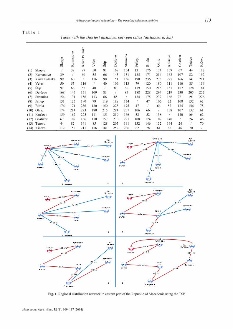
Vehicle routing and scheduling – The traveling salesman problem 113
Маш. инж. науч. спис., 32 (1), 109–117 (2014)
T a b l e 1 Table with the shortest distances between cities (distances in km)
Skop
je
Kum
anov
o
Kriv
a Pa
lank
a
Vel
es
Štip
Delče
vo
Stru
mic
a
Prile
p
Bito
la
Ohr
id
Kru
ševo
Gos
tivar
Teto
vo
Kič
evo
(1) Skopje / 39 99 50 91 168 154 131 176 174 159 67 44 112 (2) Kumanovo 39 / 60 55 66 145 131 135 171 214 162 107 82 152 (3) Kriva Palanka 99 60 / 116 90 151 156 190 236 273 225 166 141 211 (4) Veles 50 55 116 / 40 109 113 79 120 180 111 110 85 156 (5) Štip 91 66 52 40 / 83 66 119 150 215 151 157 128 181 (6) Delčevo 168 145 151 109 83 / 85 188 228 294 219 230 205 252 (7) Strumica 154 131 156 113 66 85 / 134 175 237 166 221 191 226 (8) Prilep 131 135 190 79 119 188 134 / 47 106 32 108 132 62 (9) Bitola 176 171 236 120 150 228 175 47 / 66 52 124 146 78
(10) Ohrid 174 214 273 180 215 294 237 106 66 / 138 107 132 61 (11) Kruševo 159 162 225 111 151 219 166 32 52 138 / 140 164 62 (12) Gostivar 67 107 166 110 157 230 221 108 124 107 140 / 24 46 (13) Tetovo 44 82 141 85 128 205 191 132 146 132 164 24 / 70 (14) Kičevo 112 152 211 156 181 252 266 62 78 61 62 46 70 /
Fig. 1. Regional distribution network in eastern part of the Republic of Macedonia using the TSP
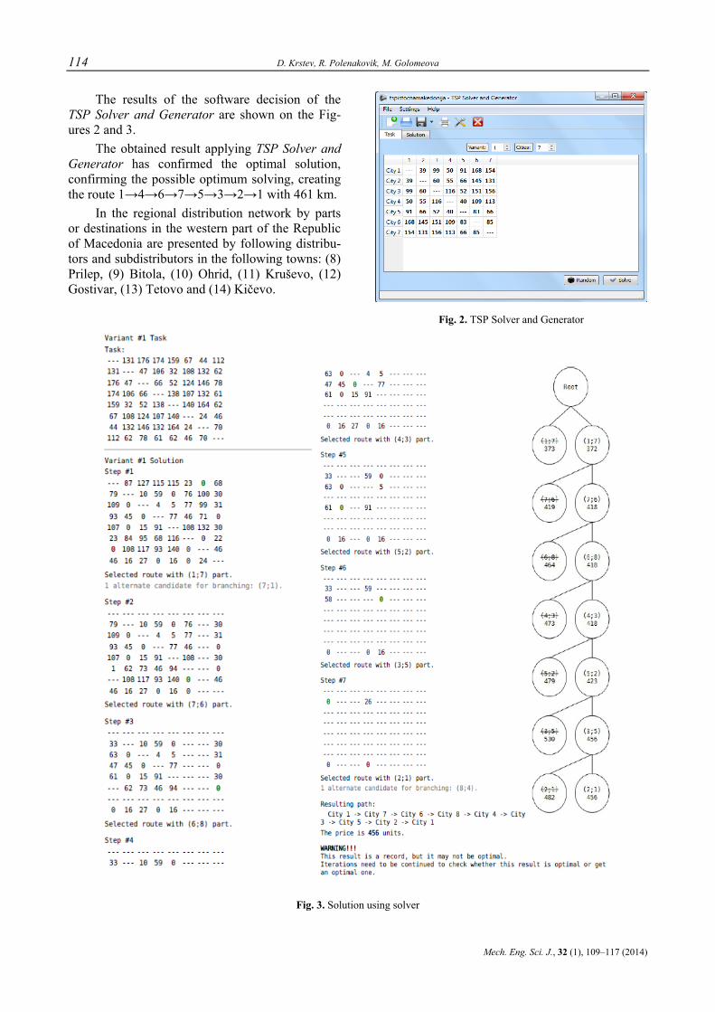
114 D. Krstev, R. Polenakovik, M. Golomeova
Mech. Eng. Sci. J., 32 (1), 109–117 (2014)
The results of the software decision of the ТSP Solver and Generator are shown on the Fig-ures 2 and 3.
The obtained result applying ТSP Solver and Generator has confirmed the optimal solution, confirming the possible optimum solving, creating the route 1→4→6→7→5→3→2→1 with 461 km.
In the regional distribution network by parts or destinations in the western part of the Republic of Macedonia are presented by following distribu-tors and subdistributors in the following towns: (8) Prilep, (9) Bitola, (10) Ohrid, (11) Kruševo, (12) Gostivar, (13) Tetovo and (14) Kičevo.
Fig. 2. ТSP Solver and Generator
Fig. 3. Solution using solver
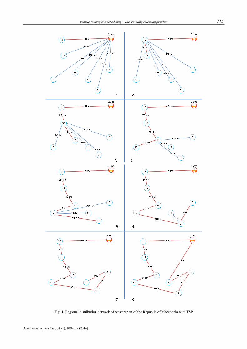
Vehicle routing and scheduling – The traveling salesman problem 115
Маш. инж. науч. спис., 32 (1), 109–117 (2014)
Fig. 4. Regional distribution network of westernpart of the Republic of Macedonia with TSP

116 D. Krstev, R. Polenakovik, M. Golomeova
Mech. Eng. Sci. J., 32 (1), 109–117 (2014)
Considering the obtained solutions for vehicle routing from the Figure 4 it’s evidently to create complete tour 1→13→12→14→10→9→8→11→ 1 which length is 479 km. But, knowing that this method don’t approach optimal value of the tour, for the second time we’ll repeat the network trying to find better tour, for example 1→13→12→14→ 10→9→11→8→1. The total distance of this tour will be 456 km, instead the previous distance of 479 km, or the difference of 23 km.
ТSP Solver and Generator. By means of the applicative software it’s possible to optimize ТЅР procedure, providing the appropriate procedure for optimal transport decision of the energetic new product L-carnitine in the region of the western part of the Republic of Macedonia. The Figure 4 has showed distances between cities where product are distrubuted from the Koding-Skopje enterprise.
The results of the software decision of the ТSP Solver and Generator are shown on the Fig-ures 5 and 6.
Fig. 5. ТSP Solver and Generator
Fig. 6. Solution using solver.

Vehicle routing and scheduling – The traveling salesman problem 117
Маш. инж. науч. спис., 32 (1), 109–117 (2014)
The obtained results by applying the ТSP Solver and Generator confirm the optimal deci-sion, obtaining the possible route 1→13→12→ 14→10→9→11→8→1 with 456 km.
6. CONCLUSIONS
For transport and distribution of new product L-carnitine, Nicholas Dege [6], is used method of Traveling Salesman Problem (TSP) for routing on eastern and western parts of Macedonia. With comparison and analysis of the mentioned method or technique it’s possible conclusion for most ade-quate or most optimal routing for distribution and transport of the product. The obtained result apply-ing ТSP Solver and Generator has confirmed the optimal solution, confirming the possible optimum solving, creating the route 1→4→6→7→5→3→2 →1 with 461 km. The obtained results by applying the ТSP Solver and Generator confirm the optimal
decision, obtaining the possible route 1→13→12 →14→10→9→1→8→1 with 456 km.
REFERENCES
[1] C. Haksever, B. Render, R. Russell, and R. Murdick: Ser-vice Management and Operations, 2nd ed. Prentice Hall: Upper Saddle River, NJ, 476–497, 2000.
[2] Dejan Krstev: Marketing mix and logistic activities for new domestic product development, Master thesis, UGD, FPTN – Štip, p. 126, 2013.
[3] O. C. Ferrell, Michael Hartline: Marketing Strategy, Cen-gage Learning, 743, 2010.
[4] Paul Fifield: Marketing Strategy: The Difference between Marketing and Markets, Elsevier/Butterworth-Heine-mann, 316, 2007.
[5] Frederick E. Webster: Industrial Marketing Strategy, John Wiley and Sons, 384 (1995).
[6] Nicholas Dege: Technology of Bottled Wather, 3nded., Wiley-Blackwall, 141–265, 2011.

Mech. Eng. Sci. J., 31 (1–2), 107–108 (2013)
Mechanical Engineering – Scientific Journal, Vol. 32, No. 1, pp. 119–120 (2014) CODEN: MINSC5 In print: ISSN 1857–5293
On line: ISSN 1875–9191
INSTRUCTIONS FOR AUTHORS
Mechanical Engineering – Scientific Journal is published twice yearly. The journal publishes original scientific papers, short communica-tions, reviews and professional papers from all fields of mechanical engineering.
The journal also publishes (continuously or occasionally) the bibliographies of the members of the Faculty, book reviews, reports on meetings, news of future meetings, important events and dates, and various rubrics, wich contribute to the development of the corresponding scientific field.
Original scientific papers should contain hitherto unpublished results of completed original scientific research. The number of pages (including tables and figures) should not exceed 15.
Short communications should also contain completed but briefly presented results of original scientific research. The number of pages should not exceed 5 (including tables and figures).
Reviews are submitted at the invitation of the Editorial Board. They should be surveys of the in-vestigations and knowledge of several authors in a given research area. The competency of the authors should be assured by their own published results.
Professional papers report on useful practi-cal results that are not original but help the results of the original scientific research to be adopted into scientific and production use. The number of pages (including tables and figures) should not exceed 10.
Acceptance for publication in the Journal obliges the authors not to publish the same re-sults elsewhere.
1. SUBMISSION
Manuscript should be submitted in triplicate, typed (1½ spaced) on A4 paper with margins of 2.5 cm on each side at the following address:
Faculty of Mechanical Engineering (Mechanical Engineering – Scientific Journal)
Editor in Chief P.O. Box 464 MK-1001 Skopje Republic of Macedonia The papers and appendices should be num-
bered. It is strongly recommended that the MS Word 2003 and/or PDF files of the manuscript be sent on the disc or by e-mail on [email protected].
A letter must accompany all submissions, clearly indicating the following: title, author(s), corresponding author’s name, address and e-mail address, suggested category of the manuscript and a suggestion of five referees (their names, e-mail and affiliation).
2. THE REVIEW PROCESS
Papers received by the Editorial Board are sent to two referees (one in the case of professional papers). The suggestions of the referees and Edito-rial Board are sent to the author(s) for further ac-tion. The corrected text should be returned to the Editorial Board as soon as possible but in not more than 30 days.
3. PREPARATION OF MANUSCRIPT
The papers should be written in the shortest possible way and without unnecessary repetition.
The original scientific papers, short commu-nications and reviews should be written in English, while the professional papers may be submitted also in Macedonian.
Only SI (Systeme Internationale d'Unites) quantities and units are to be used.
Double subscripts and superscripts should be avoided whenever possible. Thus it is better to write ν3(PO4) than
4PO3ν or exp(–E/RT) than e–E/RT.
Strokes (/) should not be used instead of parenthe-ses.

120 Instructions for authors
Mech. Eng. Sci. J., 31 (1–2) 119–120 (2013)
Figures (photographs, diagrams and sket-ches) and mathematical formulae should each be given on a separate sheet. Figures should also be inserted in the correct place in the manuscript, be-ing horizontally reduced to 8 or 16 cm. The size of the symbols for the physical quantities and units as well as the size of the numbers and letters used in the reduced figures should be comparable with the size of the letters in the main text of the paper. Dia-grams and structural formulae should be drawn in such a way (e.g. black Indian ink on white or trac-ing paper) as to permit high quality reproduction. The use of photographs should be avoided. The tables and the figures should be numbered in Ara-bic numerals (e.g. Table 1, Fig. 1). Tables and fig-ures should be self-contained, i.e. should have cap-tions making them legible without resort to the main text. The presentation of the same results in the form of tables and figures (diagrams) is not permitted.
Footnotes are also not permitted. When a large number of compounds have
been analyzed, the results should be given in tabu-lar form.
Manuscript should contain: title, author(s) full-name(s), surname(s), address and e-mail, short abstract, key words, introduction, experimental or theoretical back-ground, results and discussion, acknowledgment (if desired), references and sum-mary.
The title should correspond to the contents of the manuscript. It should be brief and informative and include the majority of the key words.
Each paper should contain an abstract that should not exceed 150 words. The abstract should include the aim of the research, the most important results and conclusions.
In the introduction only the most important previous results related to the problem in hand should be briefly reviewed and the aim and impor-tance of the research should be stated.
The experimental section should be written as a separate section and should contain a descrip-tion of the materials used and methods employed – in form which makes the results reproducible, but without detailed description of already known methods.
Manuscripts that are related to theoretical studies, instead of experimental material, should contain a sub-heading and the theoretical back-ground where the necessary details for verifying the results obtained should be stated.
The results and discussion should be given in the same section. The discussion should contain an analysis of the results and the conclusions that can be drawn.
The reference should be given in a separate section in the order in which they appear in the text. The surname of one or two authors may be given in the text, whereas in the case of more than two authors they should be quoted as, for example, Kuzinovski and collaborators [1] or Vrtanoski et al. [1].
Papers from scientific journals should be cited as follows:
[1] G. Vrtanoski, V. Dukovski, K. Yamagu-chi: Use of polymer concrete for construction ma-terials, Proc. Fac. Mech. Eng, – Skopje, 21, 1, 43–48 (2002).
Books should be cited as follows: a) Books without editor: [2] V. Georgievski: Lake metalne konstruk-
cije. Prostorni rešetkasti sistemi, Građevinska knji-ga, Beograd, 1990, pp. 134–157.
b) Books with editor: [3] M. Golay, in: Gas Chromatography, D.
Desty, ed. Butterworths, London, 1958, p. 36. Manuscripts should also contain a summary
in Macedonian at the end of the paper. The sum-mary in Macedonian for foreign authors will be prepared by the Editorial Board. The summary should contain: title, author(s) full-name(s), sur-name(s) and address, key words and abstract.
The category of the paper is proposed by the author(s) but the Editorial Board reserves for itself the right, on the basis of the referees' opinion, to make the final choice.
Proofs are sent to the author(s) to correct printers' errors. Except for this, alterations to the text are not permitted. The proofs should be re-turned to the Editorial Board in 2 days.
The author(s) will receive, free of charge, 20 reprints of every paper published in the Journal.


![Modulhandbuch Fakultat fur Maschinenwesen 5770572 ... · [MW1450] IFR-Praktikum Hubschrauber (IFR Helicopter Flight) [MW2313] Praktikum MATLAB/Simulink for Computer Aided Engineering](https://img.pdfslide.tips/doc/110x75/5d57e67088c99371268b97b1/modulhandbuch-fakultat-fur-maschinenwesen-5770572-mw1450-ifr-praktikum.jpg)