Embed Size (px)
Citation preview
MET 327 Applied Engineering II (Dynamics) Summer 2010 Handout #1 by Hejie Lin Ch 9 Moment of Inertia
1
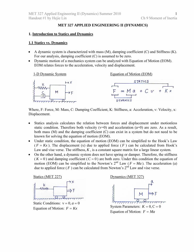
MET 327 APPLIED ENGINEERING II (DYNAMICS) 1. Introduction to Statics and Dynamics 1.1 Statics vs. Dynamics • A dynamic system is characterized with mass (M), damping coefficient (C) and Stiffness (K).
For our analysis, damping coefficient (C) is assumed to be zero. • Dynamic motion of a mechanics system can be analyzed with Equation of Motion (EOM).
EOM relates forces to the acceleration, velocity and displacement. 1-D Dynamic System
Equation of Motion (EOM)
Where, F: Force, M: Mass, C: Damping Coefficient, K: Stiffness, a: Acceleration, v: Velocity, x: Displacement. • Statics analysis calculates the relation between forces and displacement under motionless
static condition. Therefore both velocity (v=0) and acceleration (a=0) are zero. As a result, both mass (M) and the damping coefficient (C) can exist in a system but do not need to be known for solving the equation of motion (EOM).
• Under static condition, the equation of motion (EOM) can be simplified to the Hook’s Law ( KxF = ). The displacement (x) due to applied force ( F ) can be calculated from Hook’s Law and vise verse. The stiffness, K , is a constant square matrix for a large linear system.
• On the other hand, a dynamic system does not have spring or damper. Therefore, the stiffness ( 0=K ) and damping coefficient ( 0=C ) are both zero. Under this condition the equation of motion (EOM) can be simplified to the Newton’s 2nd Law ( MaF = ). The acceleration (a) due to applied force ( F ) can be calculated from Newton’s 2nd Law and vise verse.
Statics (MET 227)
Static Conditions: 0 0,v == a Equation of Motion: KxF =
Dynamics (MET 327)
System Parameters: 0C ,0 ==K Equation of Motion: MaF =
MET 327 Applied Engineering II (Dynamics) Summer 2010 Handout #1 by Hejie Lin Ch 9 Moment of Inertia
2
1.2 Statics Analysis (MET227): • Statics studies the stress and strain distribution of motionless static structures. The standard
procedures for static analysis can be described in the following two steps. Step 1: Calculate Reaction Forces and Moments • Calculate reaction forces and moments from applied forces and moments using Free Body
Diagram (FBD). All forces and moments should be balanced on any FBD. • Only force exists on a truss member because of the zero-moment points if no force acting
between the joints of the truss member. The self weight of the truss member is neglected or lumped to the end nodes (joints). Otherwise, the member should be analyzed as a beam as described as following.
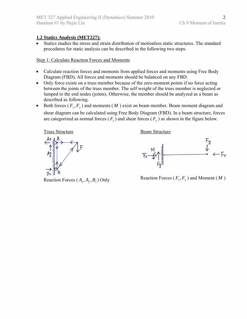
• Both forces ( yx FF , ) and moments ( M ) exist on beam member. Beam moment diagram and shear diagram can be calculated using Free Body Diagram (FBD). In a beam structure, forces are categorized as normal forces ( xF ) and shear forces ( yF ) as shown in the figure below.
Truss Structure
Reaction Forces ( xyx BAA ,, ) Only
Beam Structure
Reaction Forces ( yx FF , ) and Moment ( M )
MET 327 Applied Engineering II (Dynamics) Summer 2010 Handout #1 by Hejie Lin Ch 9 Moment of Inertia
3
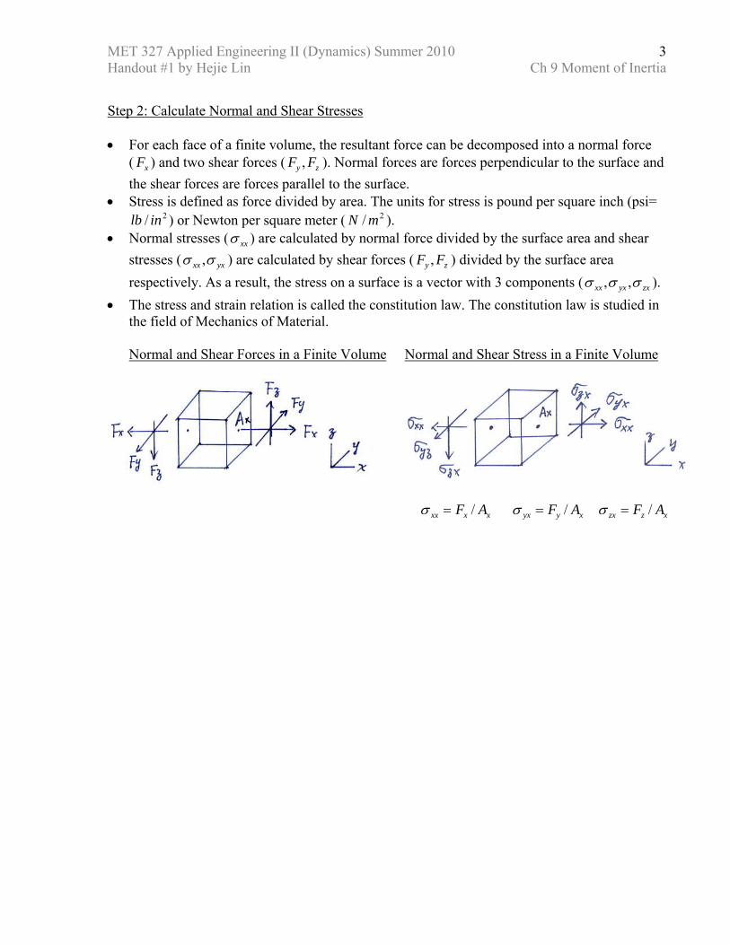
Step 2: Calculate Normal and Shear Stresses • For each face of a finite volume, the resultant force can be decomposed into a normal force
( xF ) and two shear forces ( zy FF , ). Normal forces are forces perpendicular to the surface and the shear forces are forces parallel to the surface.
• Stress is defined as force divided by area. The units for stress is pound per square inch (psi= lb / 2in ) or Newton per square meter ( N / 2m ).
• Normal stresses ( xxσ ) are calculated by normal force divided by the surface area and shear stresses ( yxxx σσ , ) are calculated by shear forces ( zy FF , ) divided by the surface area respectively. As a result, the stress on a surface is a vector with 3 components ( zxyxxx σσσ ,, ).
• The stress and strain relation is called the constitution law. The constitution law is studied in the field of Mechanics of Material.
Normal and Shear Forces in a Finite Volume
Normal and Shear Stress in a Finite Volume
xxxx AF /=σ xyyx AF /=σ xzzx AF /=σ
MET 327 Applied Engineering II (Dynamics) Summer 2010 Handout #1 by Hejie Lin Ch 9 Moment of Inertia
4
1.3 Dynamic Analysis (MET 327) • Dynamics analysis can be divided into the following two categories: Kinematics and
Kinetics. Kinematics • Kinematics studies the relationship between displacement, velocity and acceleration without
considering the mass and force of the system. (Ch. 10,11) Force and mass are not considered in Kinematics analysis.
• If we neglect the deformation of a solid body, we can consider it as a rigid body. It takes six Degree of Freedom (DOF) to fully describe a motion of a rigid body. Three translational DOF corresponds to forces and three rotational DOF corresponds to the moments.
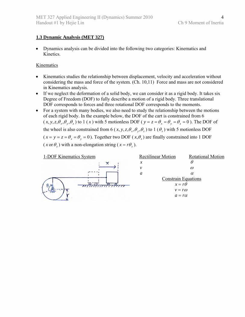
• For a system with many bodies, we also need to study the relationship between the motions of each rigid body. In the example below, the DOF of the cart is constrained from 6 ( zyxzyx θθθ ,,,,, ) to 1 ( x ) with 5 motionless DOF ( 0===== zyxzy θθθ ). The DOF of the wheel is also constrained from 6 ( zyxzyx θθθ ,,,,, ) to 1 ( zθ ) with 5 motionless DOF ( 0===== yxzyx θθ ). Together two DOF ( zx θ, ) are finally constrained into 1 DOF ( zx θor ) with a non-elongation string ( zrx θ= ).
1-DOF Kinematics System
Rectilinear Motion Rotational Motion x θ v ω a α Constrain Equations θrx = ωrv = αra =
MET 327 Applied Engineering II (Dynamics) Summer 2010 Handout #1 by Hejie Lin Ch 9 Moment of Inertia
5
Kinetics • Kinetic studies the relation between force and mass of a system. The stiffness and Damping
coefficient are zero in a dynamic analysis. • Newton’s 2nd Law is extended into rectilinear motion and rotational motion. In any Free
Body Diagram (FBD), the summation of force vectors (including applied forces, reaction forces and initial forces) will be zero.
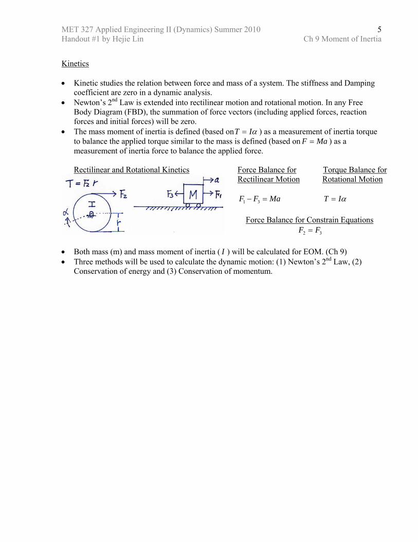
• The mass moment of inertia is defined (based on αIT = ) as a measurement of inertia torque to balance the applied torque similar to the mass is defined (based on MaF = ) as a measurement of inertia force to balance the applied force.
Rectilinear and Rotational Kinetics
Force Balance for Torque Balance for Rectilinear Motion Rotational Motion
MaFF =− 31 αIT = Force Balance for Constrain Equations 32 FF =
• Both mass (m) and mass moment of inertia ( I ) will be calculated for EOM. (Ch 9) • Three methods will be used to calculate the dynamic motion: (1) Newton’s 2nd Law, (2)
Conservation of energy and (3) Conservation of momentum.
MET 327 Applied Engineering II (Dynamics) Summer 2010 Handout #1 by Hejie Lin Ch 9 Moment of Inertia
6
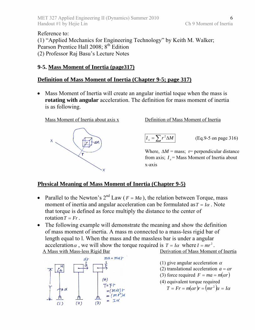
Reference to: (1) “Applied Mechanics for Engineering Technology” by Keith M. Walker; Pearson Prentice Hall 2008; 8th Edition (2) Professor Raj Basu’s Lecture Notes 9-5. Mass Moment of Inertia (page317) Definition of Mass Moment of Inertia (Chapter 9-5; page 317) • Mass Moment of Inertia will create an angular inertial toque when the mass is
rotating with angular acceleration. The definition for mass moment of inertia is as following.
Mass Moment of Inertia about axis x
Definition of Mass Moment of Inertia
∑ ∆= MrI x2 (Eq.9-5 on page 316)
Where, M∆ = mass; r= perpendicular distance from axis; xI = Mass Moment of Inertia about x-axis
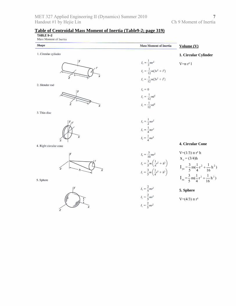
Physical Meaning of Mass Moment of Inertia (Chapter 9-5) • Parallel to the Newton’s 2nd Law ( MaF = ), the relation between Torque, mass
moment of inertia and angular acceleration can be formulated as αIT = . Note that torque is defined as force multiply the distance to the center of rotation FrT = .
• The following example will demonstrate the meaning and show the definition of mass moment of inertia. A mass m connected to a mass-less rigid bar of length equal to l. When the mass and the massless bar is under a angular accelerationα , we will show the torque required is αIT = where 2mrI = .
A Mass with Mass-less Rigid Bar
Derivation of Mass Moment of Inertia (1) give angular acceleration α (2) translational acceleration ra α= (3) force required ( )rmmaF α== (4) equivalent torque required ( ) ( ) ααα ImrrrmFrT ==== 2
MET 327 Applied Engineering II (Dynamics) Summer 2010 Handout #1 by Hejie Lin Ch 9 Moment of Inertia
7
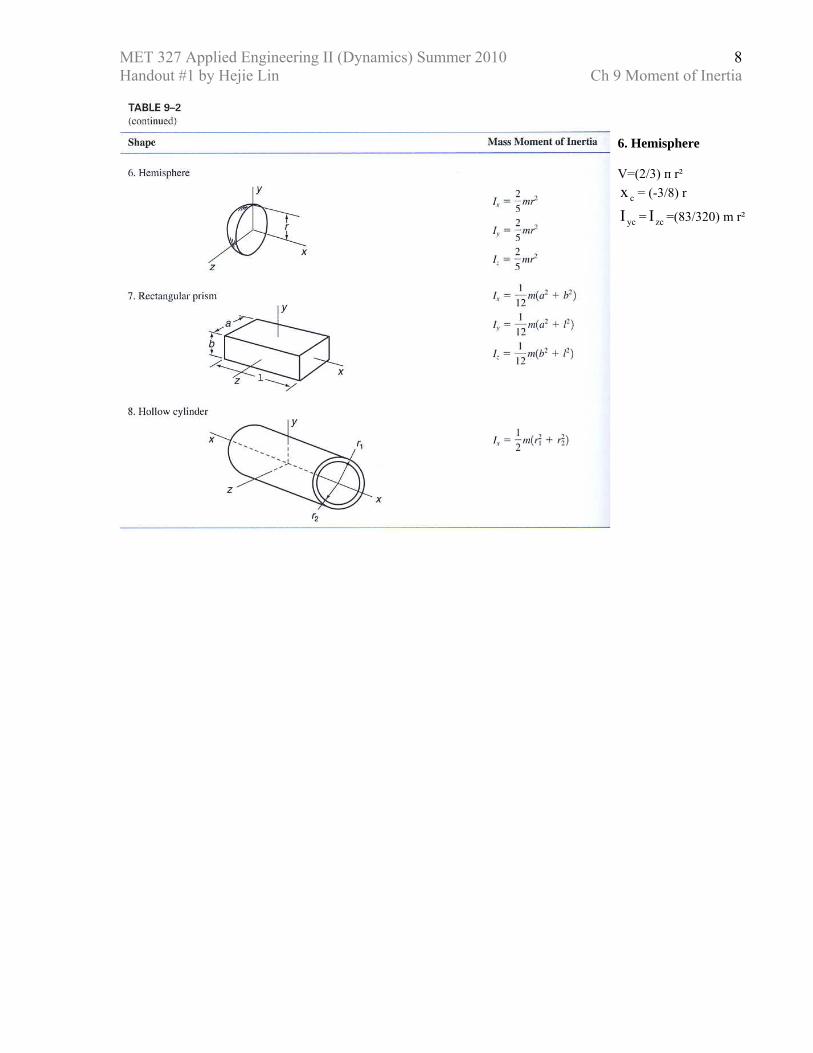
Table of Centroidal Mass Moment of Inertia (Table9-2; page 319)
Volume (V) 1. Circular Cylinder V=п r² l 4. Circular Cone V=(1/3) п r² h
cx = (3/4)h
ycI = )h161r
41m(
53 22 +
zcI = )h161r
41m(
53 22 +
5. Sphere V=(4/3) п r²
MET 327 Applied Engineering II (Dynamics) Summer 2010 Handout #1 by Hejie Lin Ch 9 Moment of Inertia
8
6. Hemisphere V=(2/3) п r²
cx = (-3/8) r
ycI = zcI =(83/320) m r²
MET 327 Applied Engineering II (Dynamics) Summer 2010 Handout #1 by Hejie Lin Ch 9 Moment of Inertia
9
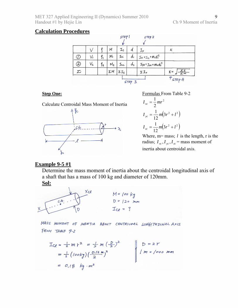
Calculation Procedures
Step One: Calculate Centroidal Mass Moment of Inertia
Formulas From Table 9-2
( )
( )22
22
2
3121
312121
lrmI
lrmI
mrI
zc
yc
xc
+=
+=
=
Where, m= mass; l is the length, r is the radius; zcycxc III ,, = mass moment of inertia about centroidal axis.
Example 9-5 #1
Determine the mass moment of inertia about the centroidal longitudinal axis of a shaft that has a mass of 100 kg and diameter of 120mm. Sol:
MET 327 Applied Engineering II (Dynamics) Summer 2010 Handout #1 by Hejie Lin Ch 9 Moment of Inertia
10
Units of Mass Moment of Inertia (Chapter 9-5) • The most confusion part of dealing with S.I. units and British units in the mass. Mass is a
very important quantity in the dynamic analysis. Both S.I. and British units are used in Canada and the U.S.
S.I. Units British Units
M=mass Kg (= N·s²/m) slug (= lb·s²/ ft) r =perpendicular distance from axis m ft
xI = mass moment of inertia Kg·m² (= N·m·s²) slug·ft² (= lb·ft·s²) T=torque N·m lb·ft
F=Force N (= Kg·m/s²) lb (= slug·ft/s²) a=acceleration m/s² ft/s² α =angular acceleration rad/s² rad/s² • In S.I. system, mass (Kg) is the basic units and force Newton (N) is a derived units. • In British system, force or more precisely weight (lb) is the basic units and the mass (slug)
is the derived units. • Note that, g = gravity acceleration = 9.81 m/s² = 32.2 ft/s². Therefore, the gravity force
acting on 1 Kg mass is 9.81 N, and the gravity force acting on 1 slug mass is 32.2 lb. W=M·g 9.81 Kg·m/s² = (1 Kg) (9.81 m/ s²) 32.2 lb= (1 lb·s²/ ft) (32.2 ft/s²) However, it is conventionally to replace Kg·m/s² with N and replace lb·s²/ ft with slug. That is Kg·m/s² = N (Force Units) lb·s²/ ft = slug (Mass Units) The same equations is therefore more commonly presented as 9.81 N = (1 Kg) (9.81 m/ s²) 32.2 lb= (1 slug) (32.2 ft/s²) For example, something weighted 10 lb will be equal to M=W/g= (10 lb)/ (32.2 ft/s²)= 0.31 lb·s²/ ft = 0.31 slug
MET 327 Applied Engineering II (Dynamics) Summer 2010 Handout #1 by Hejie Lin Ch 9 Moment of Inertia
11
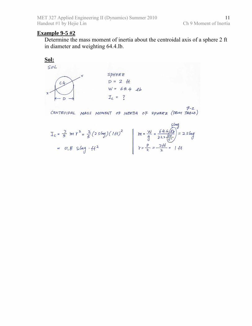
Example 9-5 #2 Determine the mass moment of inertia about the centroidal axis of a sphere 2 ft in diameter and weighting 64.4.lb. Sol:
MET 327 Applied Engineering II (Dynamics) Summer 2010 Handout #1 by Hejie Lin Ch 9 Moment of Inertia
12
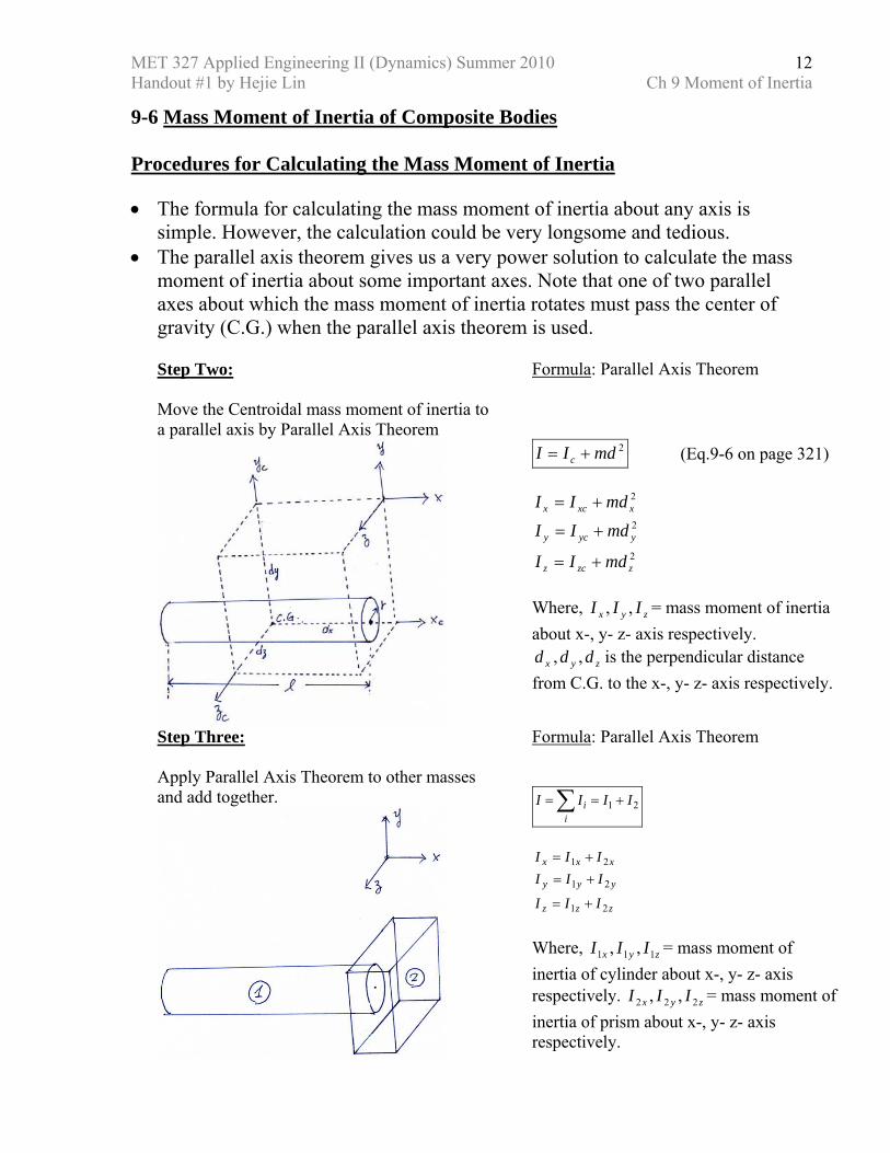
9-6 Mass Moment of Inertia of Composite Bodies Procedures for Calculating the Mass Moment of Inertia • The formula for calculating the mass moment of inertia about any axis is
simple. However, the calculation could be very longsome and tedious. • The parallel axis theorem gives us a very power solution to calculate the mass
moment of inertia about some important axes. Note that one of two parallel axes about which the mass moment of inertia rotates must pass the center of gravity (C.G.) when the parallel axis theorem is used.
Step Two: Move the Centroidal mass moment of inertia to a parallel axis by Parallel Axis Theorem
Formula: Parallel Axis Theorem
2mdII c += (Eq.9-6 on page 321)
2
2
2
zzcz
yycy
xxcx
mdII
mdII
mdII
+=
+=
+=
Where, zyx III ,, = mass moment of inertia about x-, y- z- axis respectively.
zyx ddd ,, is the perpendicular distance from C.G. to the x-, y- z- axis respectively.
Step Three: Apply Parallel Axis Theorem to other masses and add together.
Formula: Parallel Axis Theorem
21 IIIIi
i +==∑
zzz
yyy
xxx
III
IIIIII
21
21
21
+=
+=+=
Where, zyx III 111 ,, = mass moment of inertia of cylinder about x-, y- z- axis respectively. zyx III 222 ,, = mass moment of inertia of prism about x-, y- z- axis respectively.
MET 327 Applied Engineering II (Dynamics) Summer 2010 Handout #1 by Hejie Lin Ch 9 Moment of Inertia
13
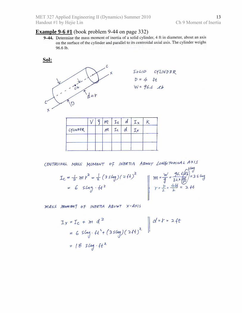
Example 9-6 #1 (book problem 9-44 on page 332)
Sol:
MET 327 Applied Engineering II (Dynamics) Summer 2010 Handout #1 by Hejie Lin Ch 9 Moment of Inertia
14
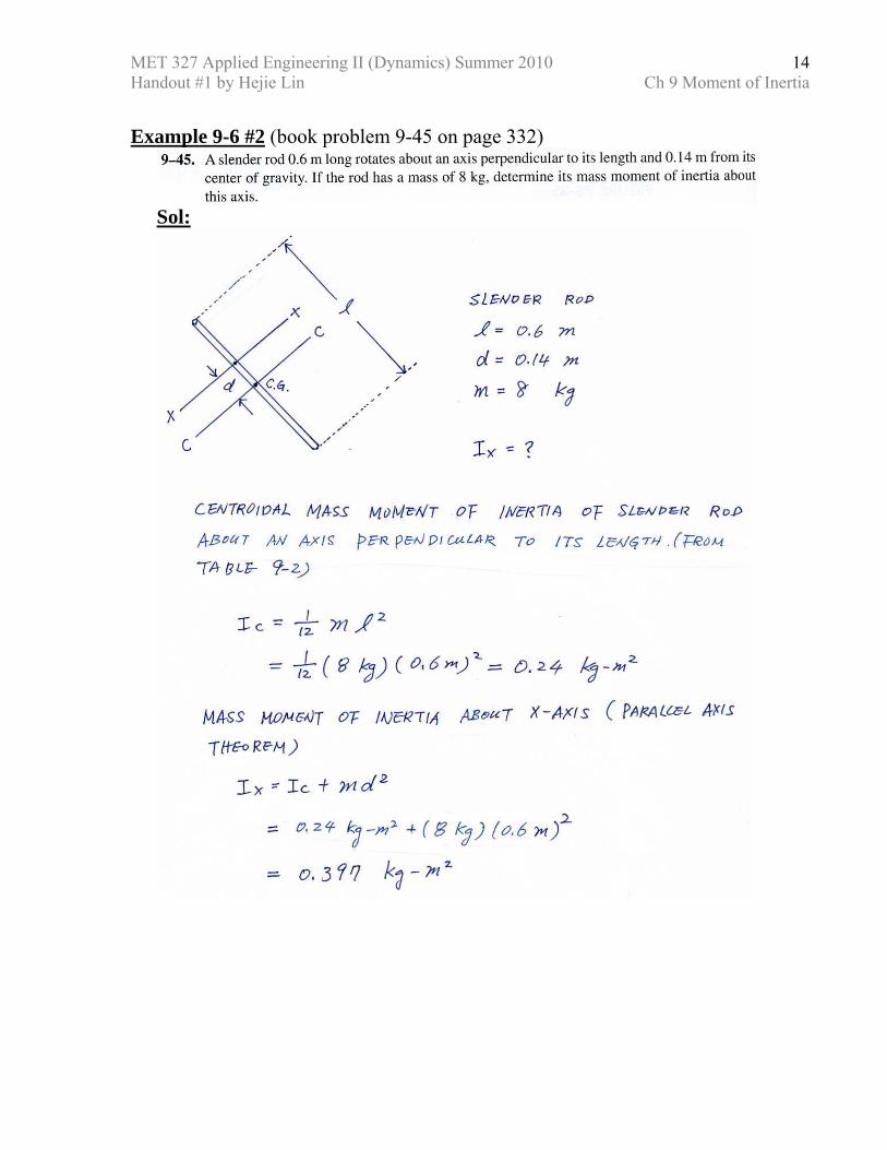
Example 9-6 #2 (book problem 9-45 on page 332)
Sol:
MET 327 Applied Engineering II (Dynamics) Summer 2010 Handout #1 by Hejie Lin Ch 9 Moment of Inertia
15
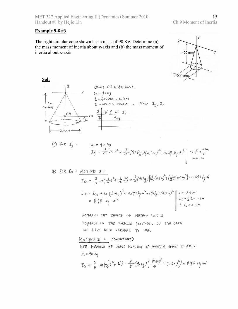
Example 9-6 #3 The right circular cone shown has a mass of 90 Kg. Determine (a) the mass moment of inertia about y-axis and (b) the mass moment of inertia about x-axis
Sol:
MET 327 Applied Engineering II (Dynamics) Summer 2010 Handout #1 by Hejie Lin Ch 9 Moment of Inertia
16
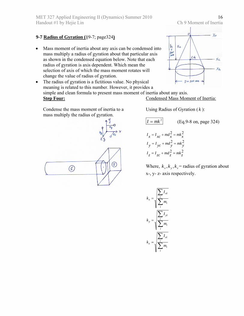
9-7 Radius of Gyration (§9-7; page324) • Mass moment of inertia about any axis can be condensed into
mass multiply a radius of gyration about that particular axis as shown in the condensed equation below. Note that each radius of gyration is axis dependent. Which mean the selection of axis of which the mass moment rotates will change the value of radius of gyration.
• The radius of gyration is a fictitious value. No physical meaning is related to this number. However, it provides a simple and clean formula to present mass moment of inertia about any axis. Step Four: Condense the mass moment of inertia to a mass multiply the radius of gyration.
Condensed Mass Moment of Inertia: Using Radius of Gyration ( k ):
2mkI = (Eq.9-8 on, page 324)
22
22
22
zmkzmdzcIzI
ymkymdycIyI
xmkxmdxcIxI
=+=
=+=
=+=
Where, zyx kkk ,, = radius of gyration about x-, y- z- axis respectively.
∑∑
∑∑
∑∑
=
=
=
ii
izi
z
ii
iyi
y
ii
ixi
x
m
Ik
m
Ik
m
Ik
MET 327 Applied Engineering II (Dynamics) Summer 2010 Handout #1 by Hejie Lin Ch 9 Moment of Inertia
17
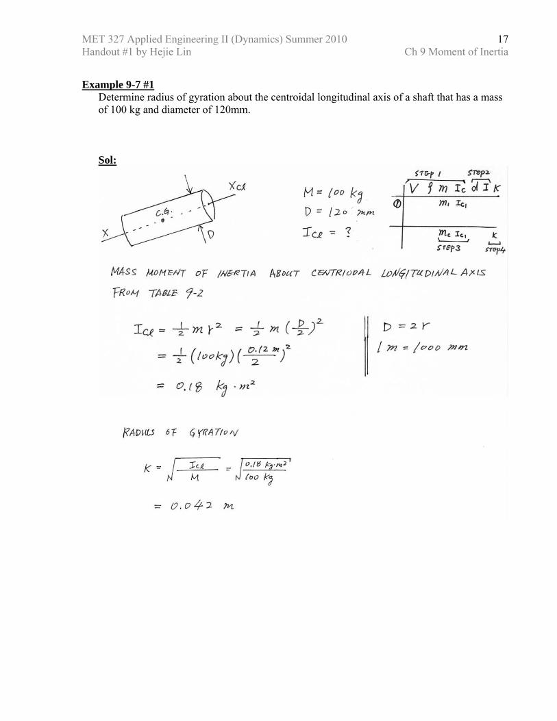
Example 9-7 #1
Determine radius of gyration about the centroidal longitudinal axis of a shaft that has a mass of 100 kg and diameter of 120mm. Sol:
MET 327 Applied Engineering II (Dynamics) Summer 2010 Handout #1 by Hejie Lin Ch 9 Moment of Inertia
18
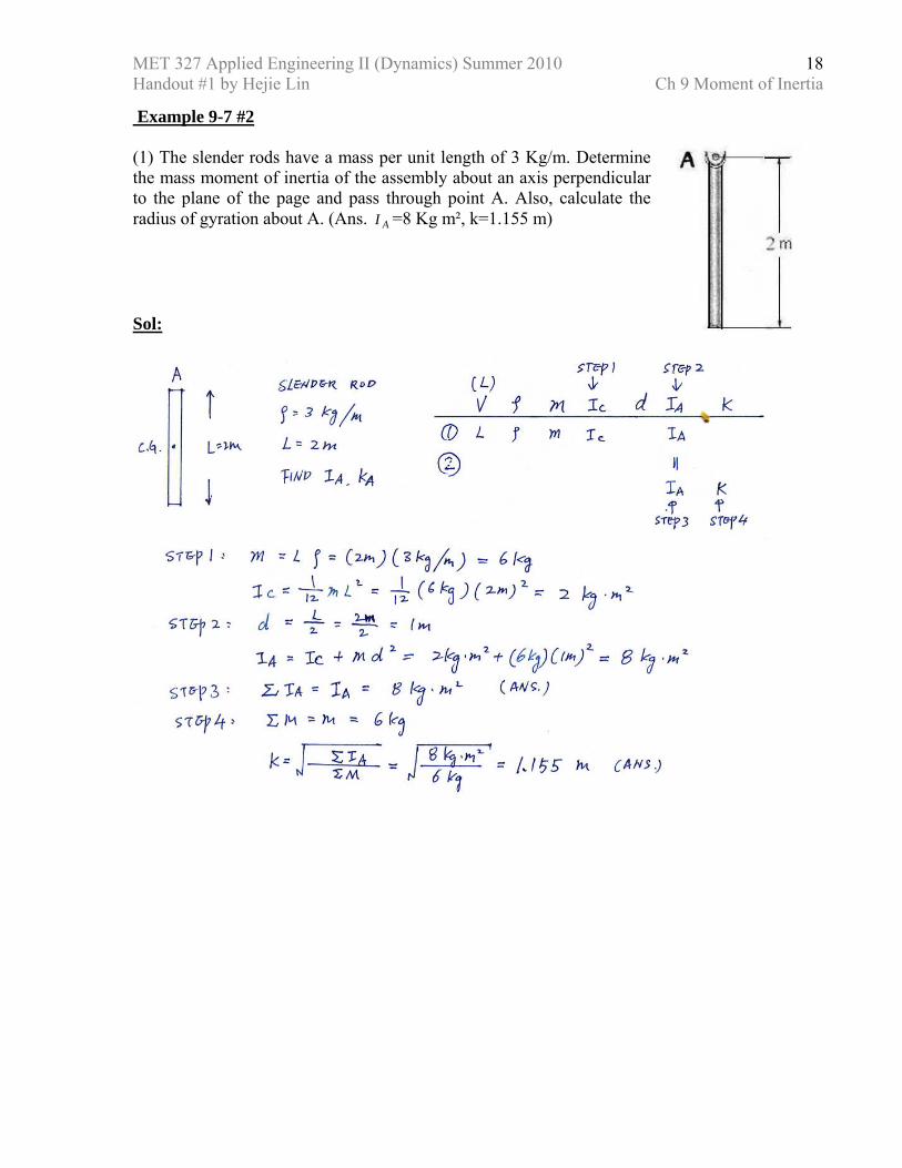
Example 9-7 #2 (1) The slender rods have a mass per unit length of 3 Kg/m. Determine the mass moment of inertia of the assembly about an axis perpendicular to the plane of the page and pass through point A. Also, calculate the radius of gyration about A. (Ans. AI =8 Kg m², k=1.155 m) Sol:
MET 327 Applied Engineering II (Dynamics) Summer 2010 Handout #1 by Hejie Lin Ch 9 Moment of Inertia
19
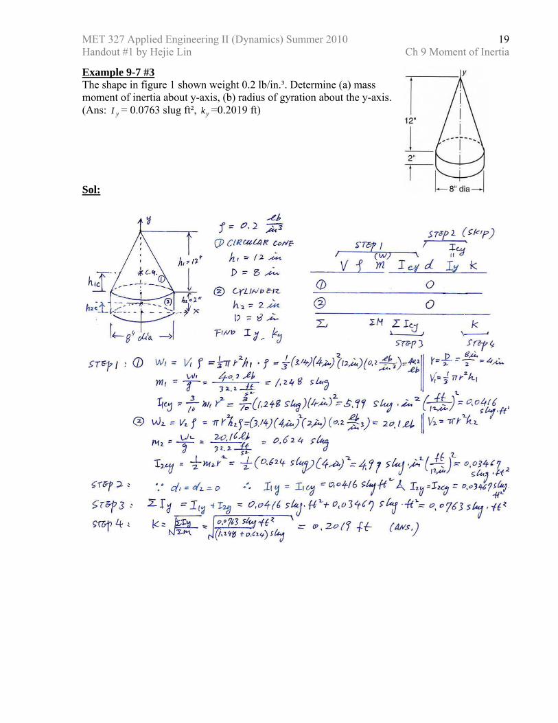
Example 9-7 #3 The shape in figure 1 shown weight 0.2 lb/in.³. Determine (a) mass moment of inertia about y-axis, (b) radius of gyration about the y-axis. (Ans: yI = 0.0763 slug ft², yk =0.2019 ft) Sol:

MET 327 Applied Engineering II (Dynamics) Summer 2010 Handout #1 by Hejie Lin Ch 9 Moment of Inertia
20
Example 9-7 #4 A fly wheel can be considered as being composed of a thin disc and a rim. The rim weights 322 lb and has diameter of 24 in. and 30 in. The disc weight 64.4 lb. Determine the mass moment of inertia about the centroidal axis about which the flywheel rotates (b) the radius of gyration about the same centroidal axis. Sol:
MET 327 Applied Engineering II (Dynamics) Summer 2010 Handout #1 by Hejie Lin Ch 9 Moment of Inertia
21
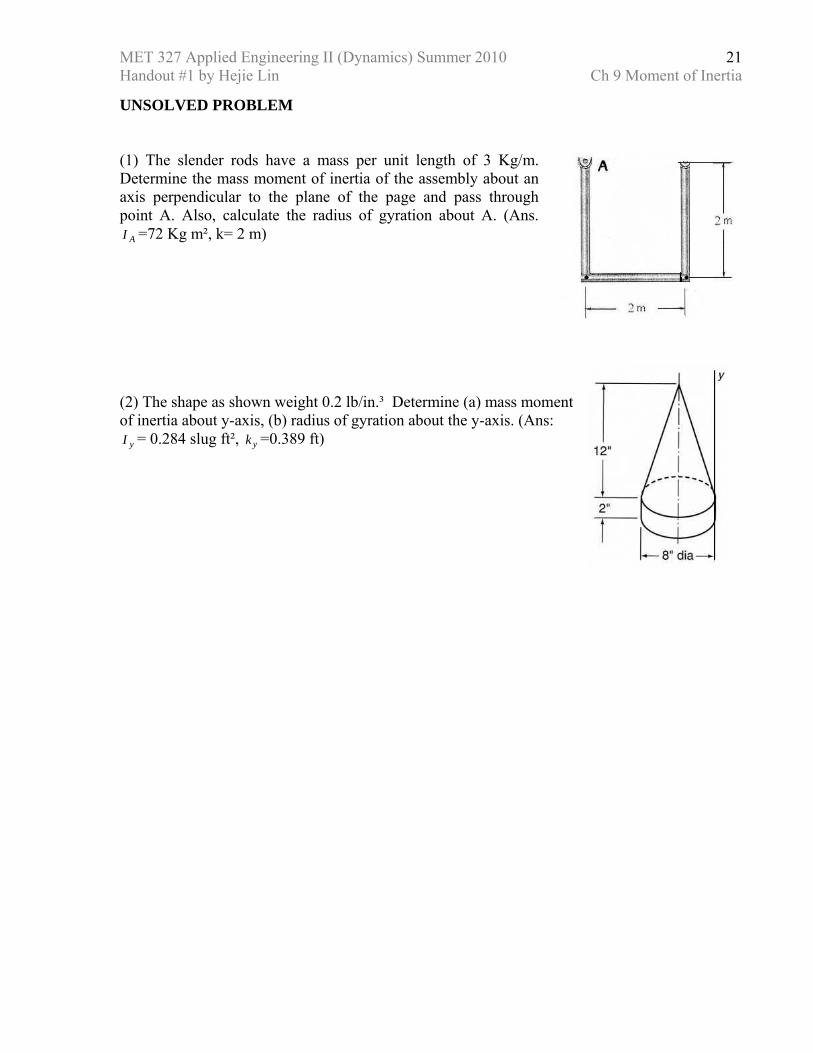
UNSOLVED PROBLEM (1) The slender rods have a mass per unit length of 3 Kg/m. Determine the mass moment of inertia of the assembly about an axis perpendicular to the plane of the page and pass through point A. Also, calculate the radius of gyration about A. (Ans.
AI =72 Kg m², k= 2 m) (2) The shape as shown weight 0.2 lb/in.³ Determine (a) mass moment of inertia about y-axis, (b) radius of gyration about the y-axis. (Ans:
yI = 0.284 slug ft², yk =0.389 ft)
MET 327 Applied Engineering II (Dynamics) Summer 2010 Handout #2 by Hejie Lin Ch10 Kinematics: Rectilinear Motion
22
Reference to: (1) “Applied Mechanics for Engineering Technology” by Keith M. Walker; Pearson Prentice Hall 2008; 8th Edition (2) Professor Raj Basu’s Lecture Notes Chapter 10. Kinematics: Rectilinear Motion (page337) Introduction • A dynamic system is characterized with mass (M), damping coefficient (C) and
Stiffness (K). For our analysis, damping coefficient (C) is assumed to be zero. • Dynamic motion of a mechanics system can be analyzed with Equation of Motion
(EOM). EOM relates forces to the acceleration, velocity and displacement. • Statics analysis calculates the relation between forces and displacement under
motionless static condition. Therefore both velocity (v=0) and acceleration (a=0) are zero. As a result, both mass (M) and the damping coefficient (C) can exist in a system but do not need to be known for solving the equation of motion (EOM).
• Under static condition, the equation of motion (EOM) can be simplified to the Hook’s Law ( KxF = ). The displacement (x) due to applied force ( F ) can be calculated from Hook’s Law and vise verse. The stiffness, K , is a constant square matrix for a large linear system.
• On the other hand, a dynamic system does not have spring or damper. Therefore, the stiffness ( 0=K ) and damping coefficient ( 0=C ) are both zero. Under this condition the equation of motion (EOM) can be simplified to the Newton’s 2nd Law ( MaF = ). The acceleration (a) due to applied force ( F ) can be calculated from Newton’s 2nd Law and vise verse.
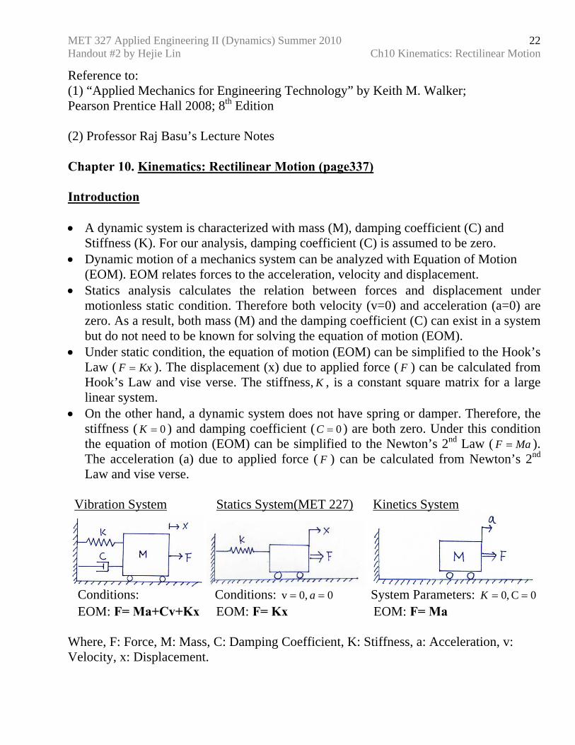
Vibration System Statics System(MET 227) Kinetics System
Conditions: Conditions: 0 0,v == a System Parameters: 0C ,0 ==K EOM: F= Ma+Cv+Kx EOM: F= Kx EOM: F= Ma Where, F: Force, M: Mass, C: Damping Coefficient, K: Stiffness, a: Acceleration, v: Velocity, x: Displacement.
MET 327 Applied Engineering II (Dynamics) Summer 2010 Handout #2 by Hejie Lin Ch10 Kinematics: Rectilinear Motion
23
• Kinematics studies the relationship between displacement, velocity and acceleration
without considering the mass and force of the system. (Ch. 10,11) Force and mass are not considered in Kinematics analysis.
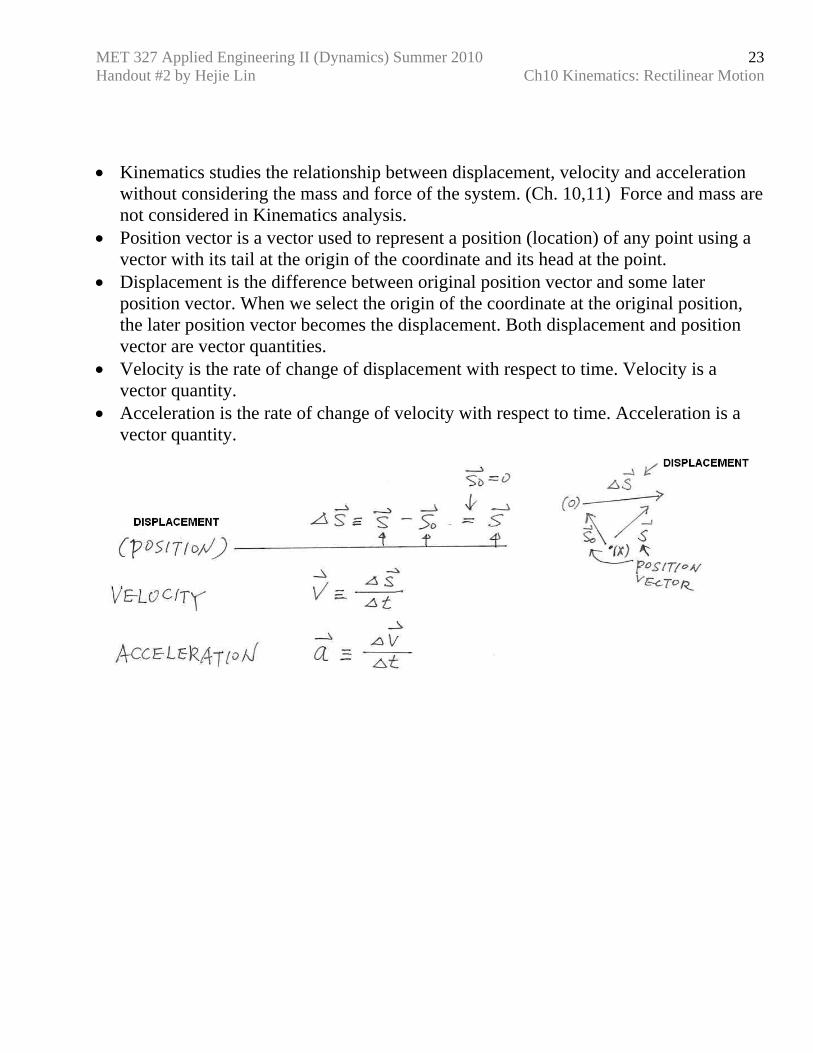
• Position vector is a vector used to represent a position (location) of any point using a vector with its tail at the origin of the coordinate and its head at the point.
• Displacement is the difference between original position vector and some later position vector. When we select the origin of the coordinate at the original position, the later position vector becomes the displacement. Both displacement and position vector are vector quantities.
• Velocity is the rate of change of displacement with respect to time. Velocity is a vector quantity.
• Acceleration is the rate of change of velocity with respect to time. Acceleration is a vector quantity.
MET 327 Applied Engineering II (Dynamics) Summer 2010 Handout #2 by Hejie Lin Ch10 Kinematics: Rectilinear Motion
24
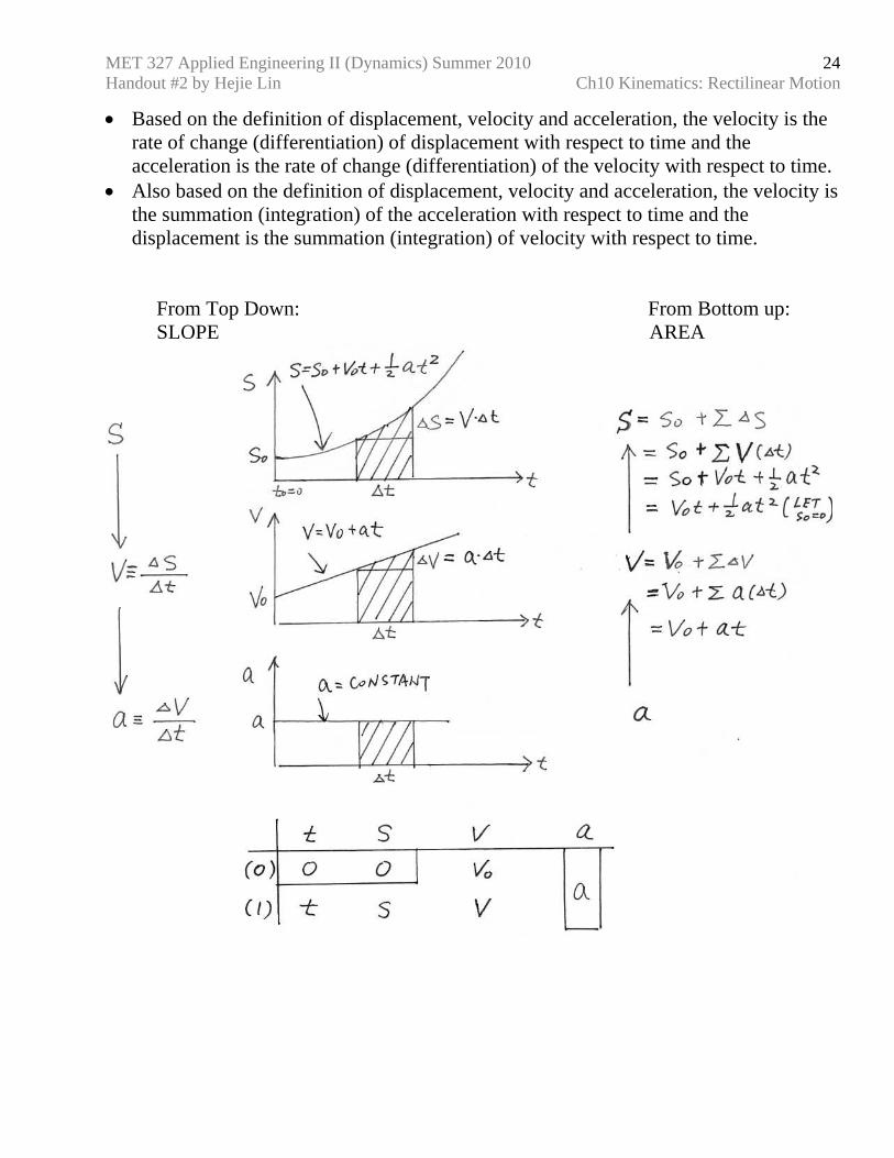
• Based on the definition of displacement, velocity and acceleration, the velocity is the rate of change (differentiation) of displacement with respect to time and the acceleration is the rate of change (differentiation) of the velocity with respect to time.
• Also based on the definition of displacement, velocity and acceleration, the velocity is the summation (integration) of the acceleration with respect to time and the displacement is the summation (integration) of velocity with respect to time.
From Top Down: From Bottom up: SLOPE AREA
MET 327 Applied Engineering II (Dynamics) Summer 2010 Handout #2 by Hejie Lin Ch10 Kinematics: Rectilinear Motion
25
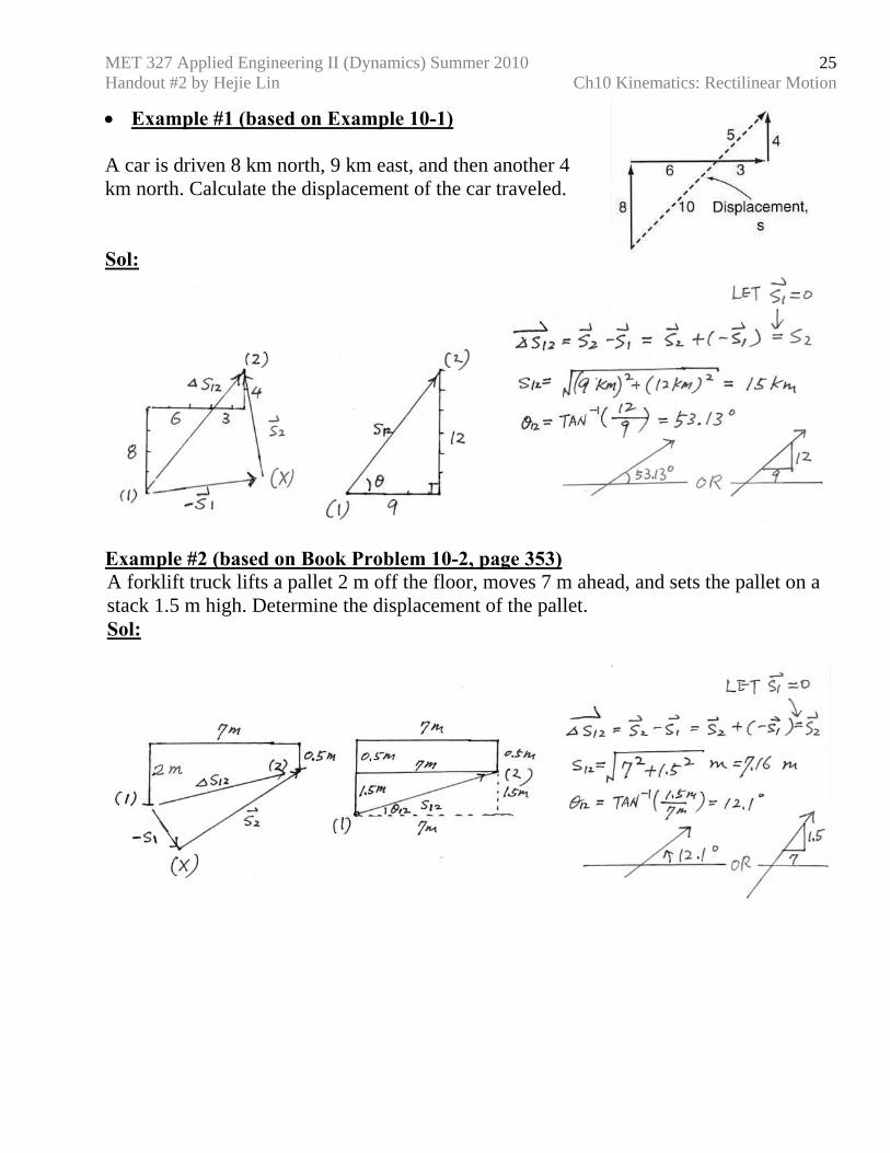
• Example #1 (based on Example 10-1) A car is driven 8 km north, 9 km east, and then another 4 km north. Calculate the displacement of the car traveled. Sol:
Example #2 (based on Book Problem 10-2, page 353) A forklift truck lifts a pallet 2 m off the floor, moves 7 m ahead, and sets the pallet on a stack 1.5 m high. Determine the displacement of the pallet. Sol:
MET 327 Applied Engineering II (Dynamics) Summer 2010 Handout #2 by Hejie Lin Ch10 Kinematics: Rectilinear Motion
26
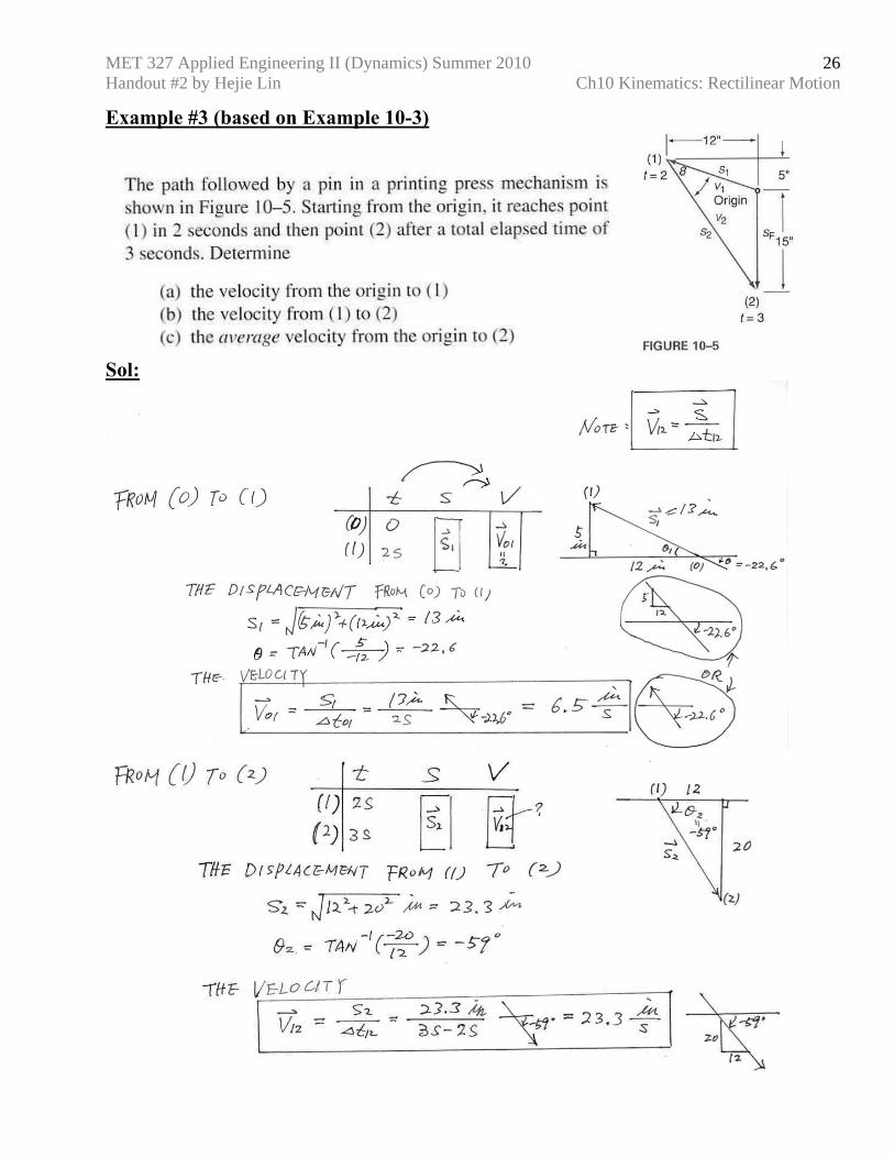
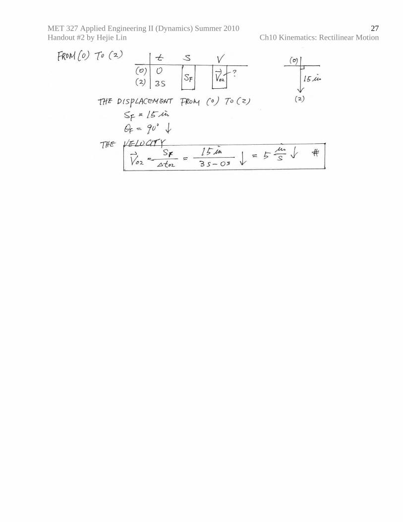
Example #3 (based on Example 10-3)
Sol:
MET 327 Applied Engineering II (Dynamics) Summer 2010 Handout #2 by Hejie Lin Ch10 Kinematics: Rectilinear Motion
27
MET 327 Applied Engineering II (Dynamics) Summer 2010 Handout #2 by Hejie Lin Ch10 Kinematics: Rectilinear Motion
28
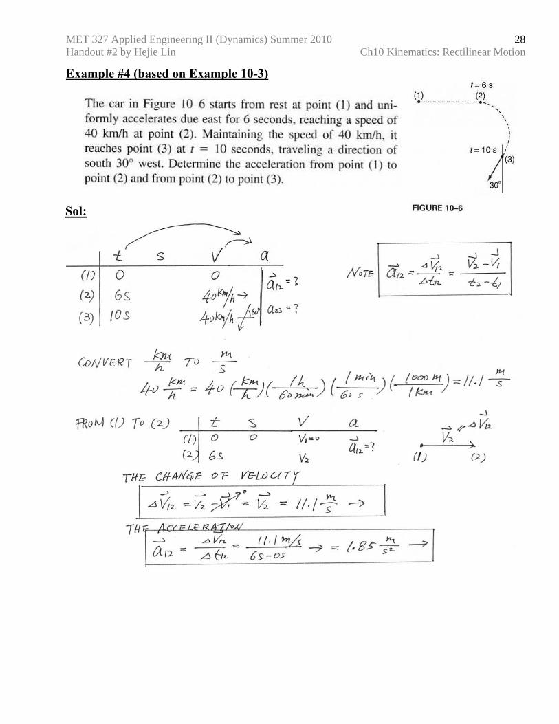
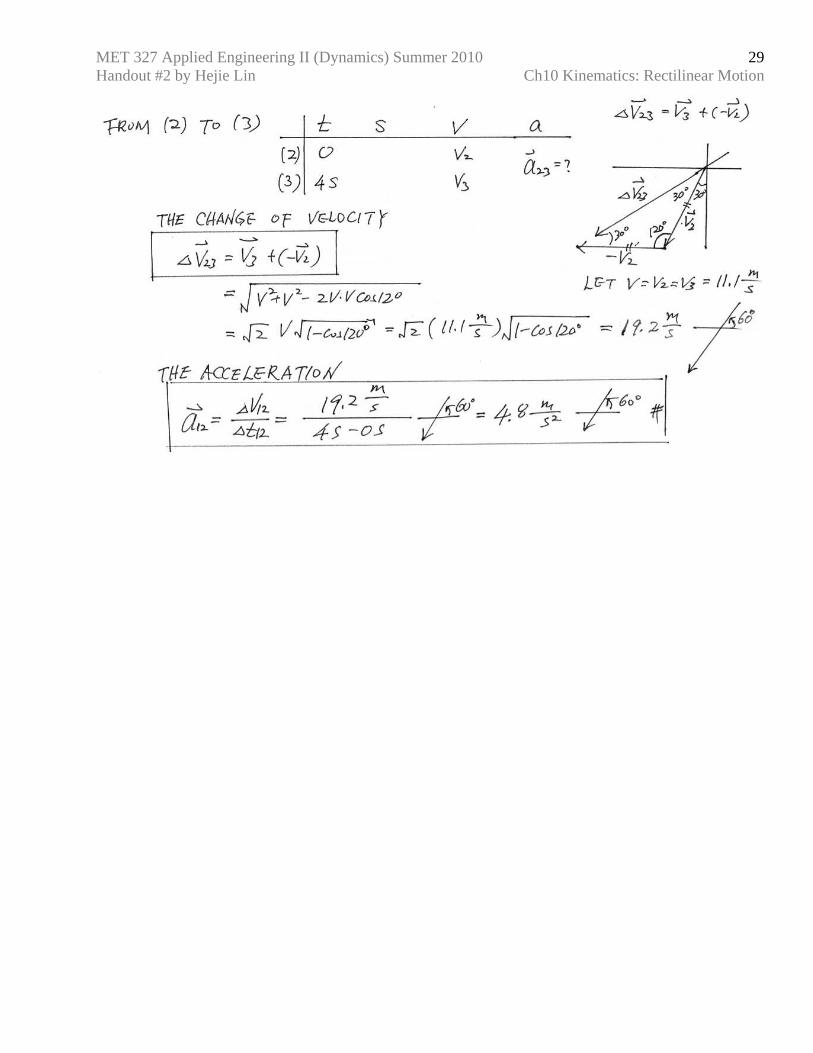
Example #4 (based on Example 10-3)
Sol:
MET 327 Applied Engineering II (Dynamics) Summer 2010 Handout #2 by Hejie Lin Ch10 Kinematics: Rectilinear Motion
29
MET 327 Applied Engineering II (Dynamics) Summer 2010 Handout #2 by Hejie Lin Ch10 Kinematics: Rectilinear Motion
30
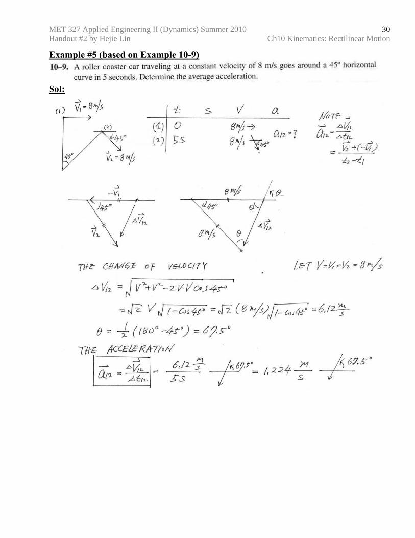
Example #5 (based on Example 10-9)
Sol:
MET 327 Applied Engineering II (Dynamics) Summer 2010 Handout #2 by Hejie Lin Ch10 Kinematics: Rectilinear Motion
31
MET 327 Applied Engineering II (Dynamics) Summer 2010 Handout #2 by Hejie Lin Ch10 Kinematics: Rectilinear Motion
32
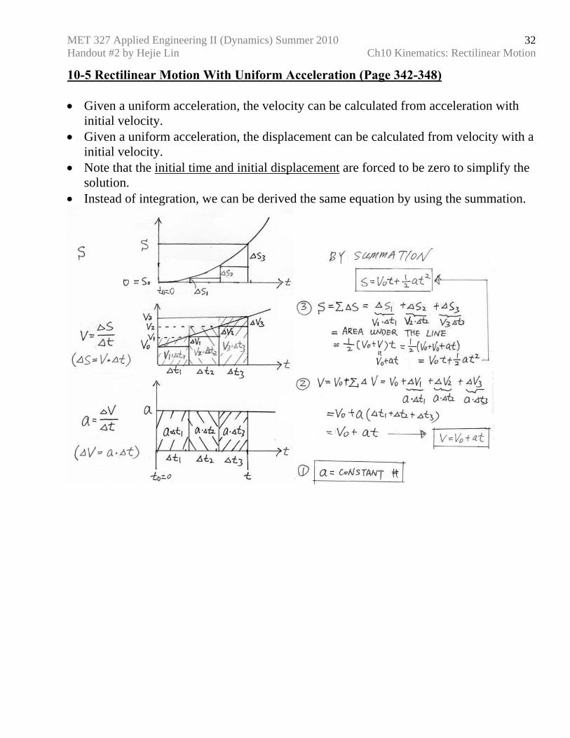
10-5 Rectilinear Motion With Uniform Acceleration (Page 342-348) • Given a uniform acceleration, the velocity can be calculated from acceleration with
initial velocity. • Given a uniform acceleration, the displacement can be calculated from velocity with a
initial velocity. • Note that the initial time and initial displacement are forced to be zero to simplify the
solution. • Instead of integration, we can be derived the same equation by using the summation.
MET 327 Applied Engineering II (Dynamics) Summer 2010 Handout #2 by Hejie Lin Ch10 Kinematics: Rectilinear Motion
33
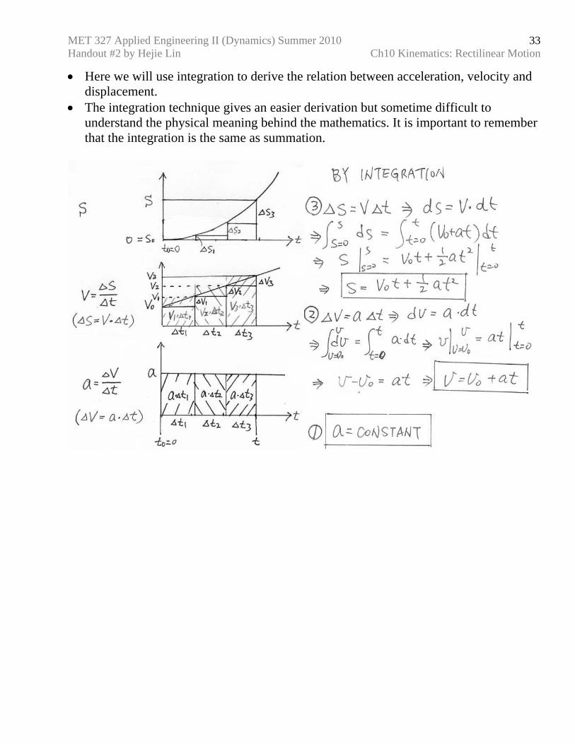
• Here we will use integration to derive the relation between acceleration, velocity and displacement.
• The integration technique gives an easier derivation but sometime difficult to understand the physical meaning behind the mathematics. It is important to remember that the integration is the same as summation.
MET 327 Applied Engineering II (Dynamics) Summer 2010 Handout #2 by Hejie Lin Ch10 Kinematics: Rectilinear Motion
34
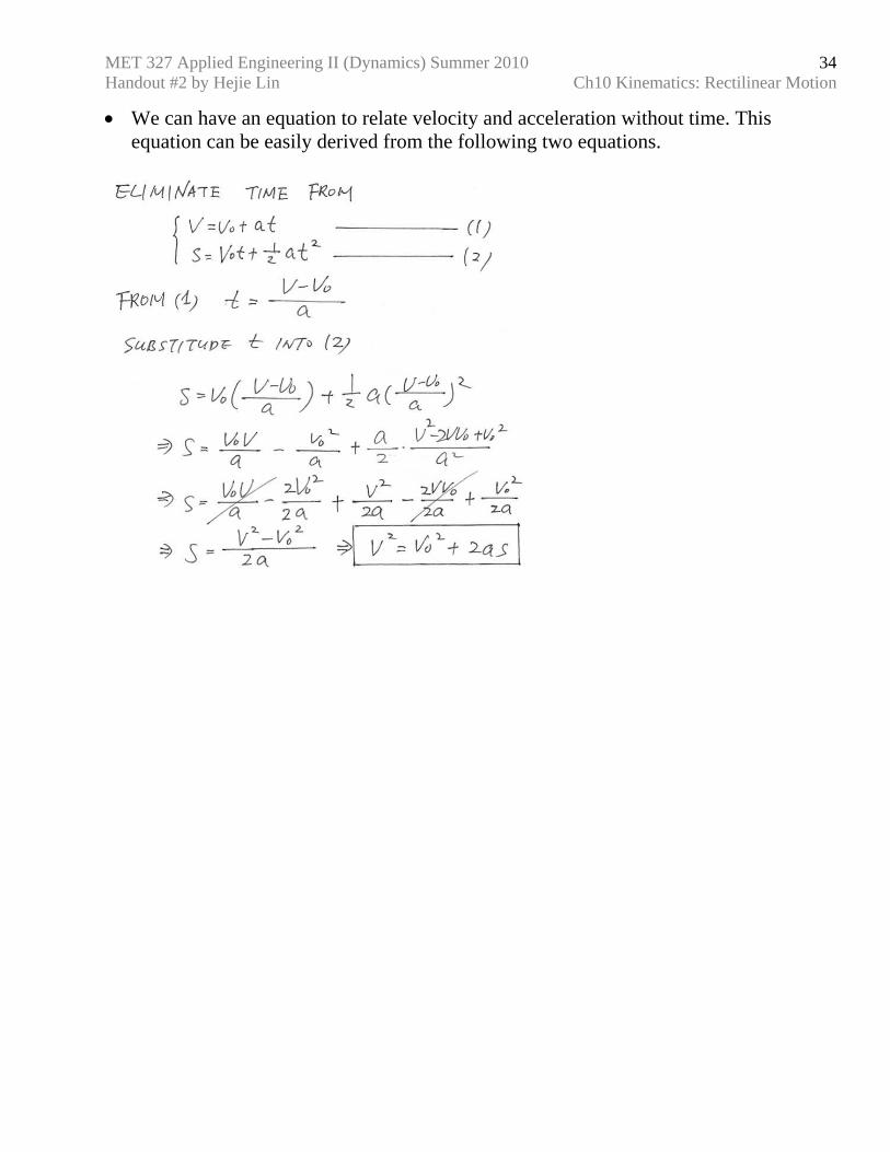
• We can have an equation to relate velocity and acceleration without time. This equation can be easily derived from the following two equations.
MET 327 Applied Engineering II (Dynamics) Summer 2010 Handout #2 by Hejie Lin Ch10 Kinematics: Rectilinear Motion
35
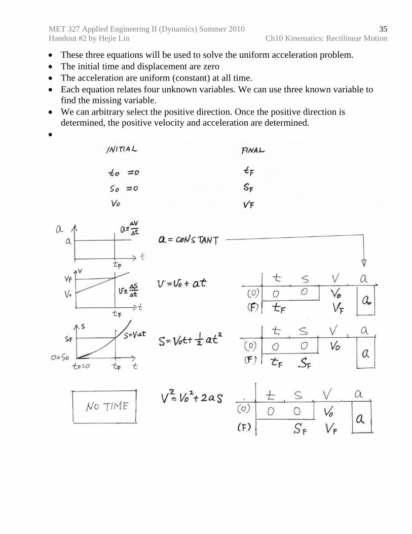
• These three equations will be used to solve the uniform acceleration problem. • The initial time and displacement are zero • The acceleration are uniform (constant) at all time. • Each equation relates four unknown variables. We can use three known variable to
find the missing variable. • We can arbitrary select the positive direction. Once the positive direction is
determined, the positive velocity and acceleration are determined. •
MET 327 Applied Engineering II (Dynamics) Summer 2010 Handout #2 by Hejie Lin Ch10 Kinematics: Rectilinear Motion
36
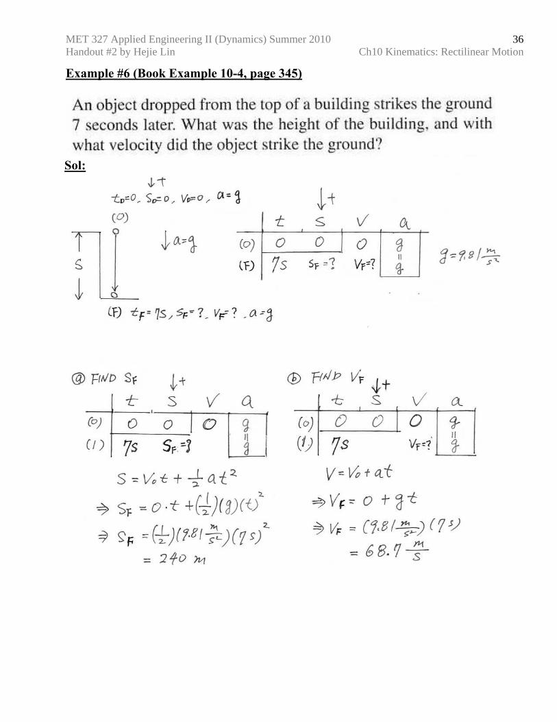
Example #6 (Book Example 10-4, page 345)
Sol:
MET 327 Applied Engineering II (Dynamics) Summer 2010 Handout #2 by Hejie Lin Ch10 Kinematics: Rectilinear Motion
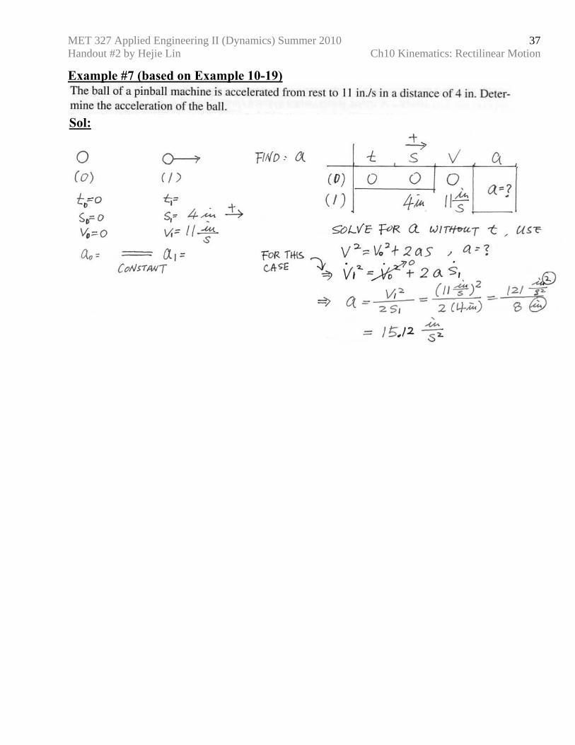
37
Example #7 (based on Example 10-19)
Sol:
MET 327 Applied Engineering II (Dynamics) Summer 2010 Handout #2 by Hejie Lin Ch10 Kinematics: Rectilinear Motion
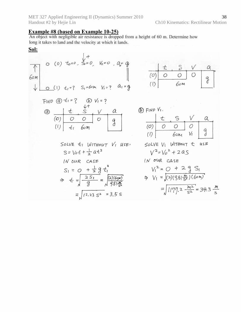
38
Example #8 (based on Example 10-25)
Sol:
MET 327 Applied Engineering II (Dynamics) Summer 2010 Handout #2 by Hejie Lin Ch10 Kinematics: Rectilinear Motion
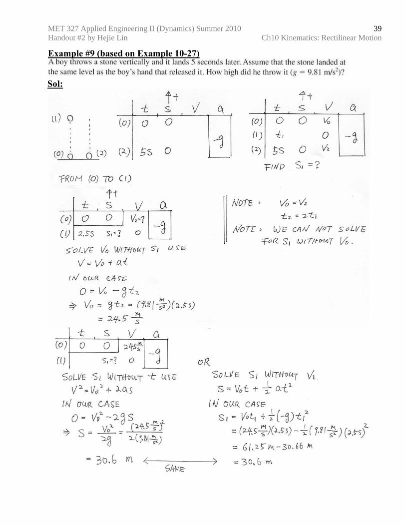
39
Example #9 (based on Example 10-27)
Sol:
MET 327 Applied Engineering II (Dynamics) Summer 2010 Handout #2 by Hejie Lin Ch10 Kinematics: Rectilinear Motion
40
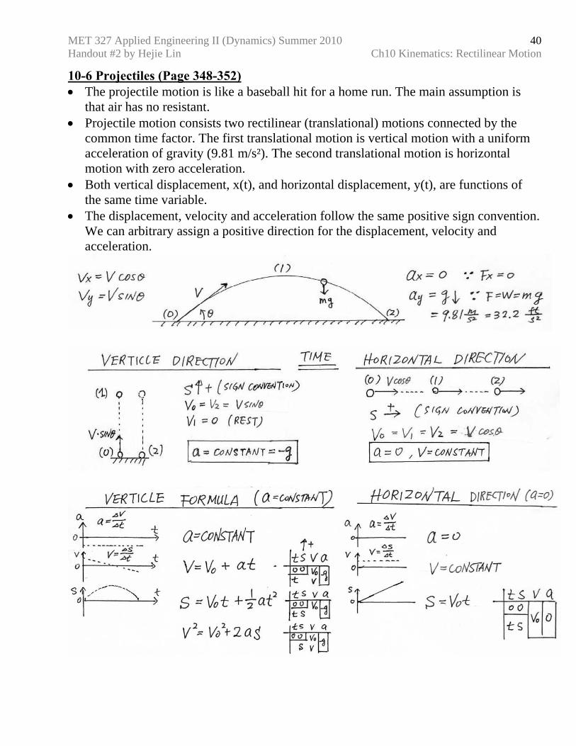
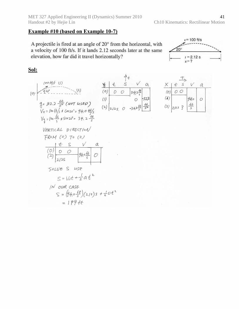
10-6 Projectiles (Page 348-352) • The projectile motion is like a baseball hit for a home run. The main assumption is
that air has no resistant. • Projectile motion consists two rectilinear (translational) motions connected by the
common time factor. The first translational motion is vertical motion with a uniform acceleration of gravity (9.81 m/s²). The second translational motion is horizontal motion with zero acceleration.
• Both vertical displacement, x(t), and horizontal displacement, y(t), are functions of the same time variable.
• The displacement, velocity and acceleration follow the same positive sign convention. We can arbitrary assign a positive direction for the displacement, velocity and acceleration.
MET 327 Applied Engineering II (Dynamics) Summer 2010 Handout #2 by Hejie Lin Ch10 Kinematics: Rectilinear Motion
41
Example #10 (based on Example 10-7)
Sol:
MET 327 Applied Engineering II (Dynamics) Summer 2010 Handout #2 by Hejie Lin Ch10 Kinematics: Rectilinear Motion
42
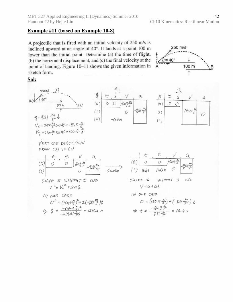
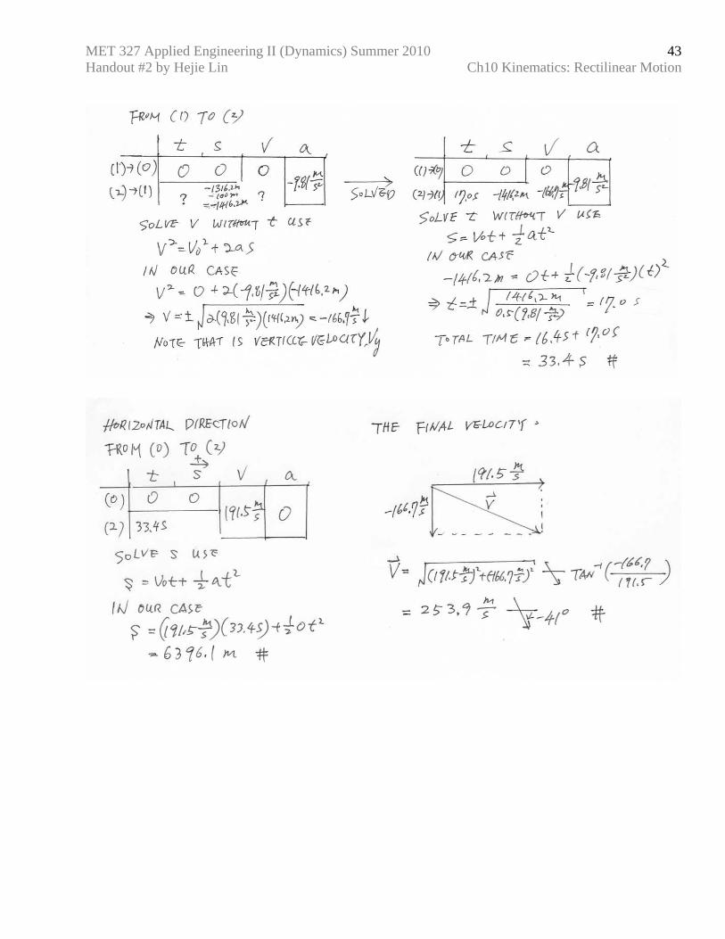
Example #11 (based on Example 10-8)
Sol:
MET 327 Applied Engineering II (Dynamics) Summer 2010 Handout #2 by Hejie Lin Ch10 Kinematics: Rectilinear Motion
43
MET 327 Applied Engineering II (Dynamics) Summer 2010 Handout #2 by Hejie Lin Ch10 Kinematics: Rectilinear Motion
44
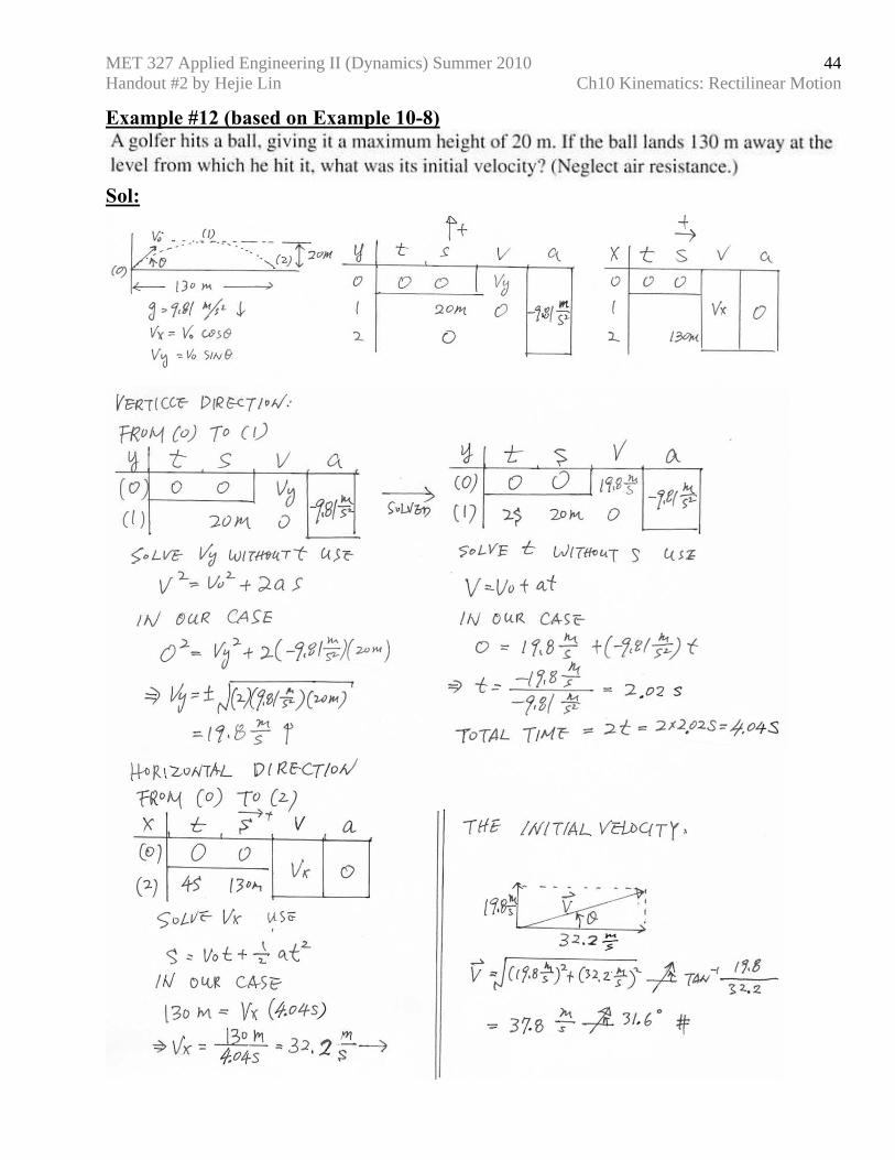
Example #12 (based on Example 10-8)
Sol:
MET 327 Applied Engineering II (Dynamics) Summer 2010 Handout #2 by Hejie Lin Ch10 Kinematics: Rectilinear Motion
45
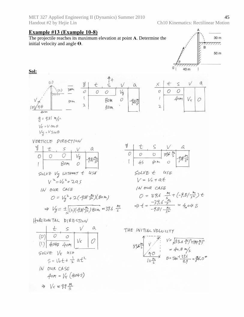
Example #13 (Example 10-8) The projectile reaches its maximum elevation at point A. Determine the initial velocity and angle Ө. Sol:
MET 327 Applied Engineering II (Dynamics) Summer 2010 Handout #2 by Hejie Lin Ch10 Kinematics: Rectilinear Motion
46
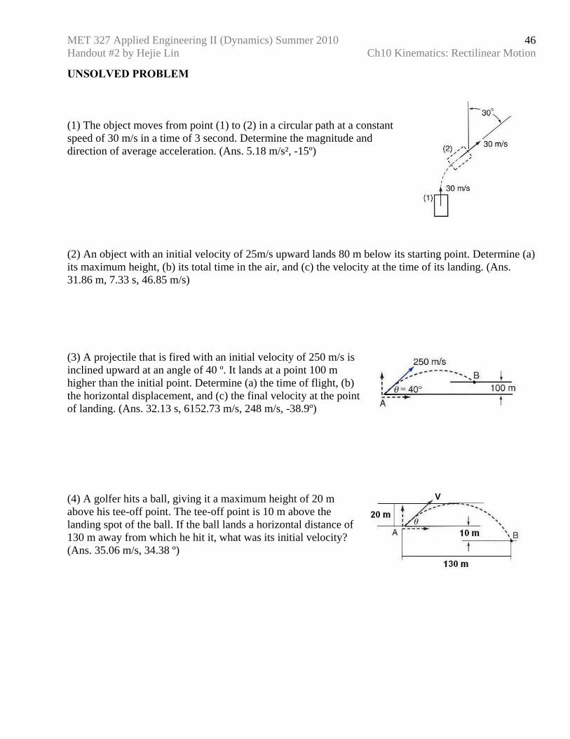
UNSOLVED PROBLEM (1) The object moves from point (1) to (2) in a circular path at a constant speed of 30 m/s in a time of 3 second. Determine the magnitude and direction of average acceleration. (Ans. 5.18 m/s², -15º) (2) An object with an initial velocity of 25m/s upward lands 80 m below its starting point. Determine (a) its maximum height, (b) its total time in the air, and (c) the velocity at the time of its landing. (Ans. 31.86 m, 7.33 s, 46.85 m/s) (3) A projectile that is fired with an initial velocity of 250 m/s is inclined upward at an angle of 40 º. It lands at a point 100 m higher than the initial point. Determine (a) the time of flight, (b) the horizontal displacement, and (c) the final velocity at the point of landing. (Ans. 32.13 s, 6152.73 m/s, 248 m/s, -38.9º) (4) A golfer hits a ball, giving it a maximum height of 20 m above his tee-off point. The tee-off point is 10 m above the landing spot of the ball. If the ball lands a horizontal distance of 130 m away from which he hit it, what was its initial velocity? (Ans. 35.06 m/s, 34.38 º)
MET 327 Applied Engineering II (Dynamics) Summer 2010 Handout #3 by Hejie Lin Ch11 Kinematics: Angular Motion
47
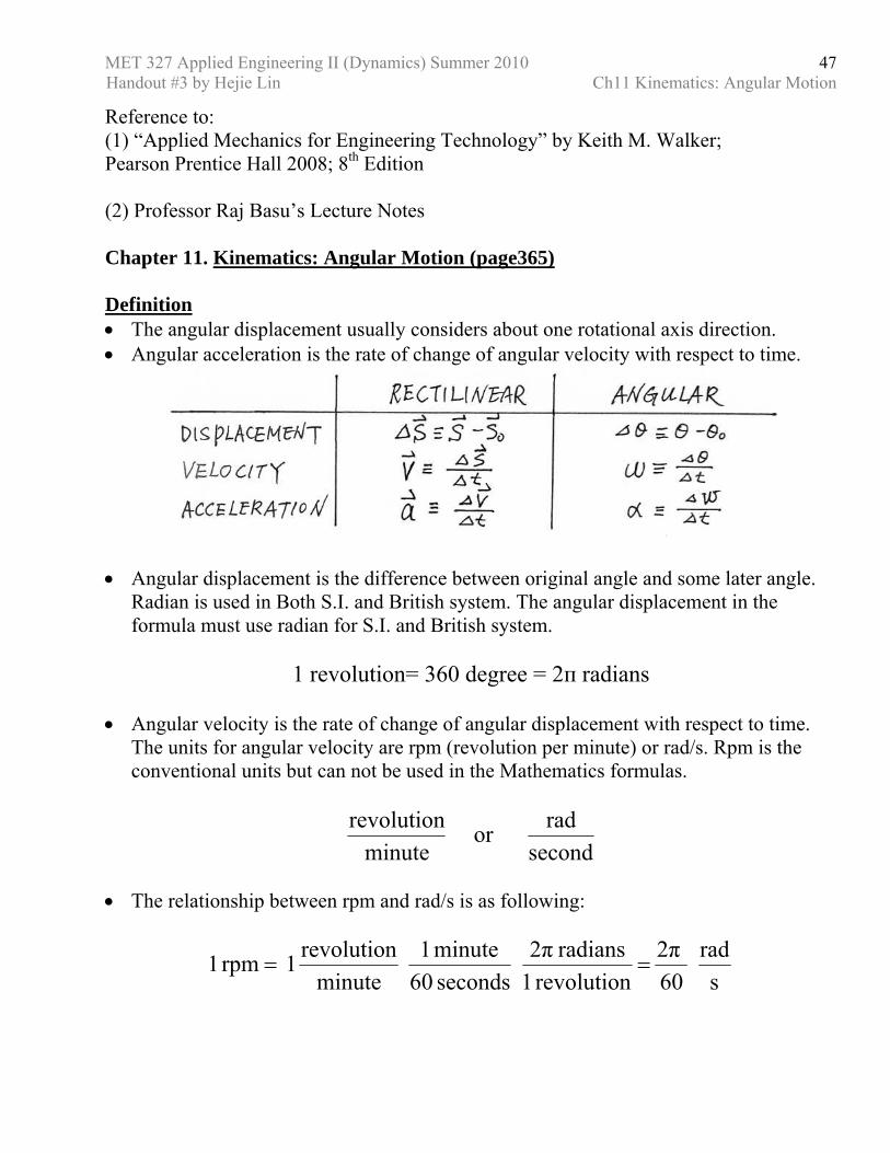
Reference to: (1) “Applied Mechanics for Engineering Technology” by Keith M. Walker; Pearson Prentice Hall 2008; 8th Edition (2) Professor Raj Basu’s Lecture Notes Chapter 11. Kinematics: Angular Motion (page365) Definition • The angular displacement usually considers about one rotational axis direction. • Angular acceleration is the rate of change of angular velocity with respect to time.
• Angular displacement is the difference between original angle and some later angle.
Radian is used in Both S.I. and British system. The angular displacement in the formula must use radian for S.I. and British system.
1 revolution= 360 degree = 2п radians
• Angular velocity is the rate of change of angular displacement with respect to time.
The units for angular velocity are rpm (revolution per minute) or rad/s. Rpm is the conventional units but can not be used in the Mathematics formulas.
secondrador
minuterevolution
• The relationship between rpm and rad/s is as following:
s
rad 60
2π revolution 1
radians 2π seconds 60minute 1
minuterevolution 1 rpm 1 ==
MET 327 Applied Engineering II (Dynamics) Summer 2010 Handout #3 by Hejie Lin Ch11 Kinematics: Angular Motion
48
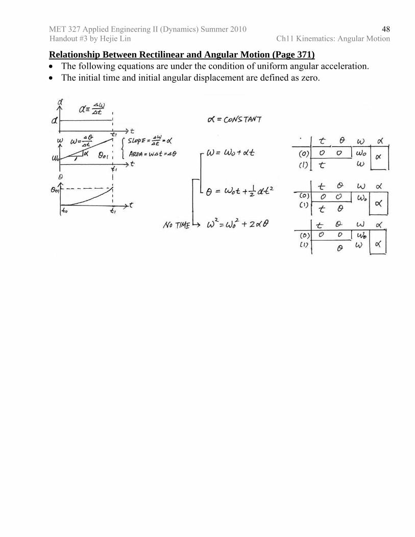
Relationship Between Rectilinear and Angular Motion (Page 371) • The following equations are under the condition of uniform angular acceleration. • The initial time and initial angular displacement are defined as zero.
MET 327 Applied Engineering II (Dynamics) Summer 2010 Handout #3 by Hejie Lin Ch11 Kinematics: Angular Motion
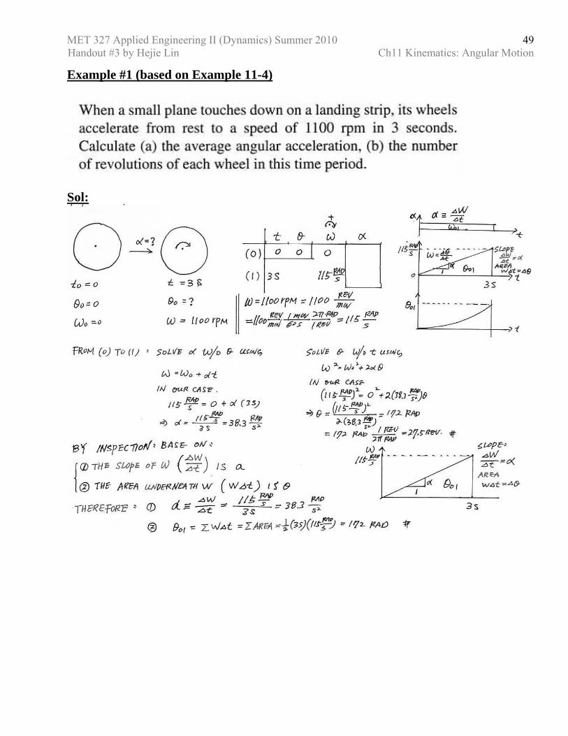
49
Example #1 (based on Example 11-4)
Sol:
MET 327 Applied Engineering II (Dynamics) Summer 2010 Handout #3 by Hejie Lin Ch11 Kinematics: Angular Motion
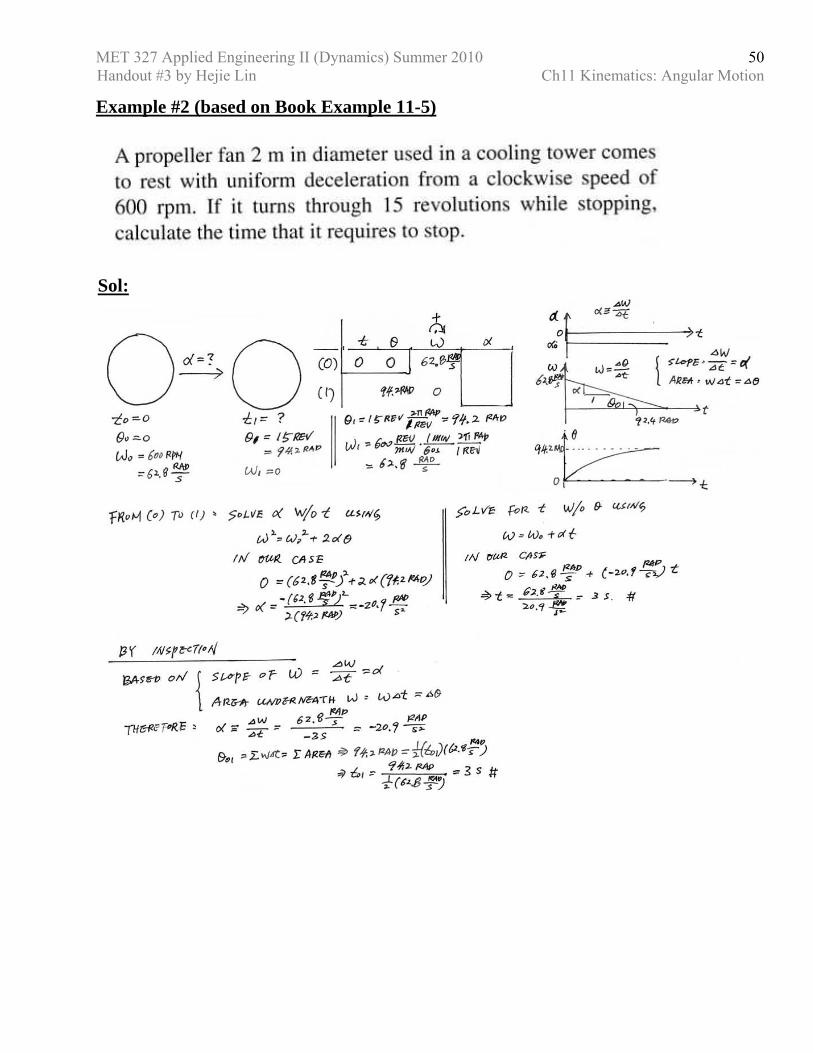
50
Example #2 (based on Book Example 11-5)
Sol:
MET 327 Applied Engineering II (Dynamics) Summer 2010 Handout #3 by Hejie Lin Ch11 Kinematics: Angular Motion
51
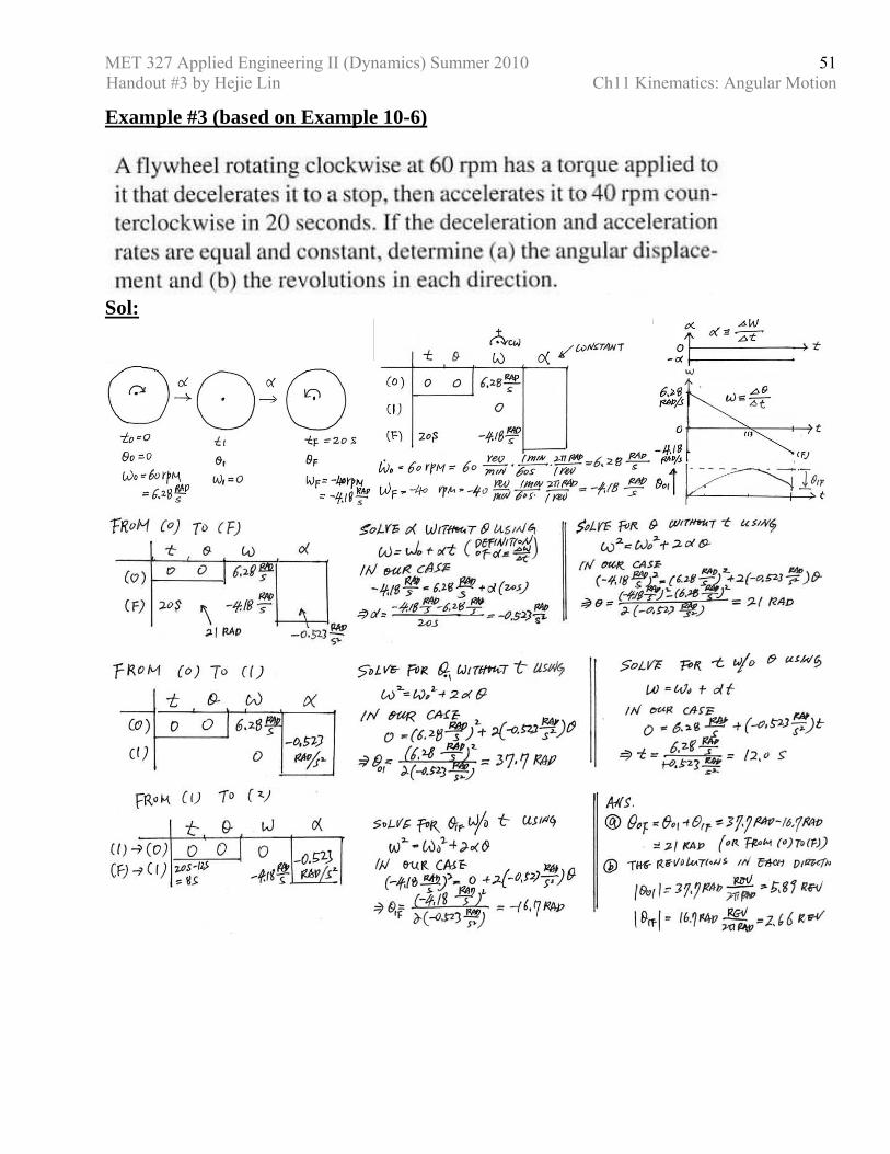
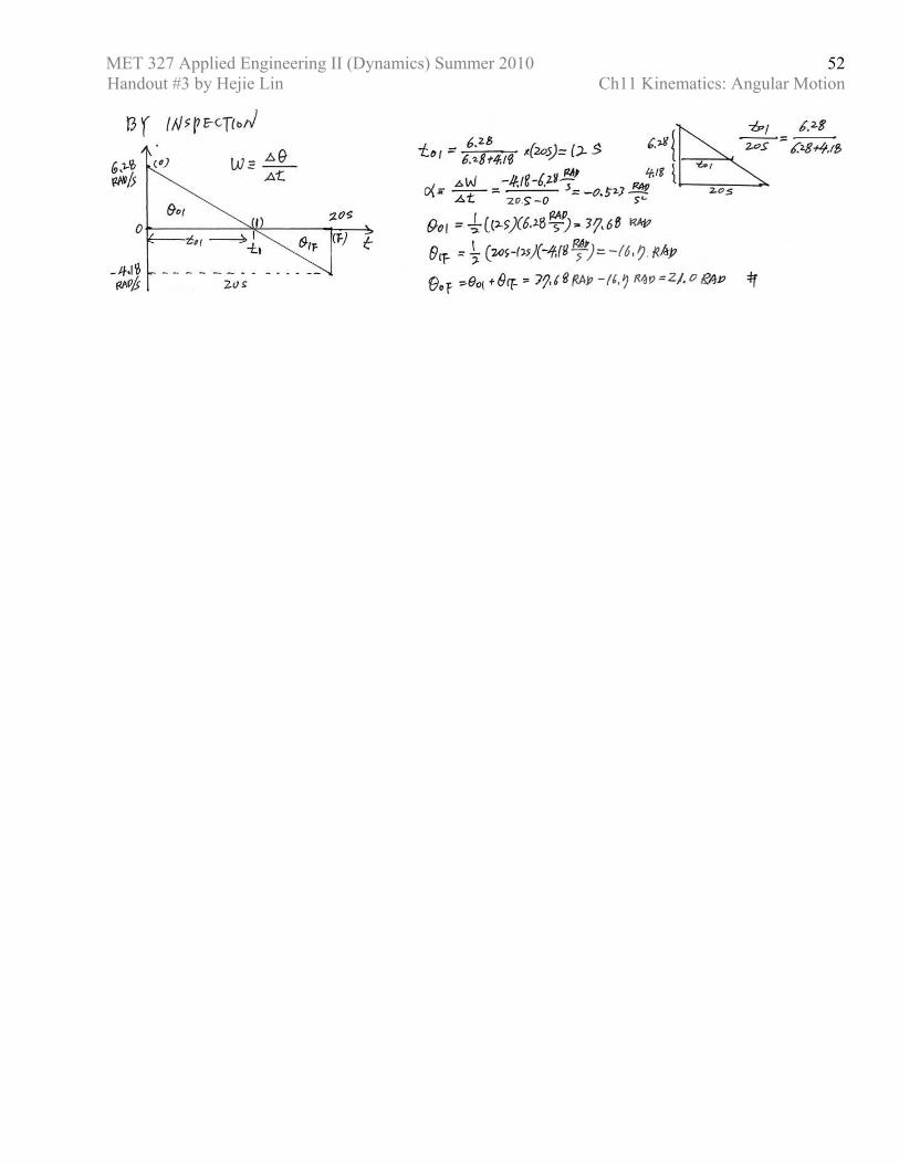
Example #3 (based on Example 10-6)
Sol:
MET 327 Applied Engineering II (Dynamics) Summer 2010 Handout #3 by Hejie Lin Ch11 Kinematics: Angular Motion
52
MET 327 Applied Engineering II (Dynamics) Summer 2010 Handout #3 by Hejie Lin Ch11 Kinematics: Angular Motion
53
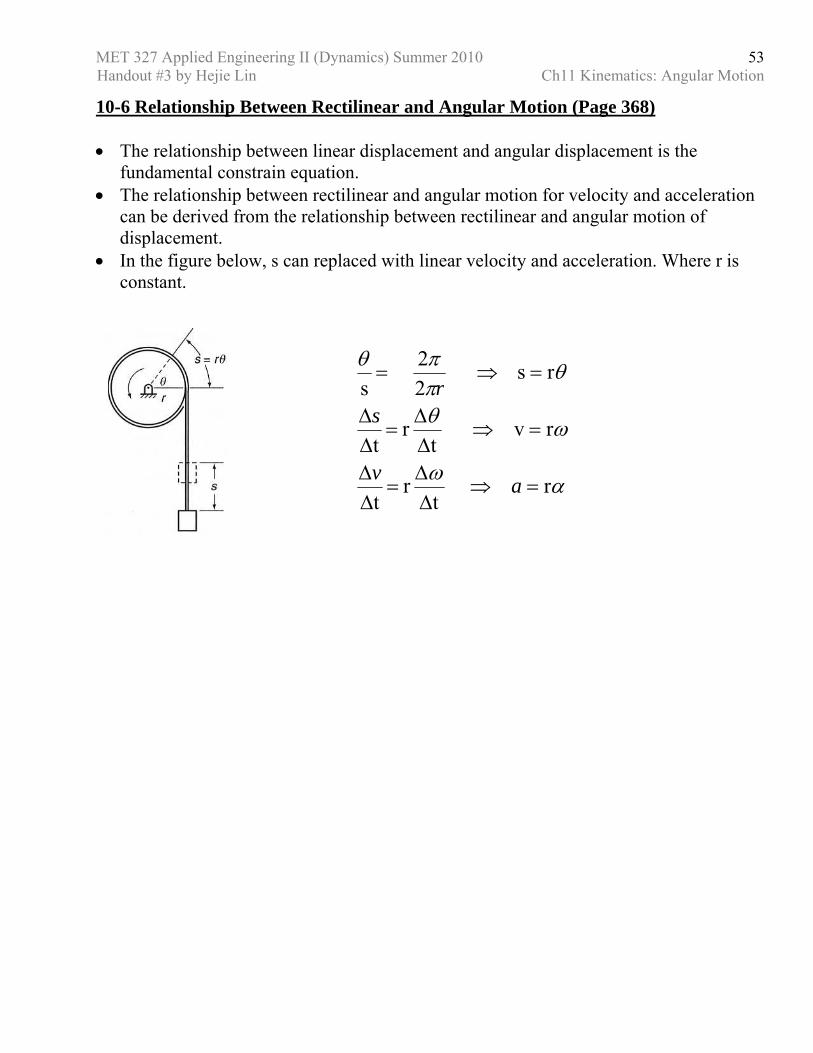
10-6 Relationship Between Rectilinear and Angular Motion (Page 368) • The relationship between linear displacement and angular displacement is the
fundamental constrain equation. • The relationship between rectilinear and angular motion for velocity and acceleration
can be derived from the relationship between rectilinear and angular motion of displacement.
• In the figure below, s can replaced with linear velocity and acceleration. Where r is constant.
αω
ωθ
θππθ
r t
r t
r v t
r t
rs 22
s
=⇒∆∆
=∆∆
=⇒∆∆
=∆∆
=⇒=
av
sr
MET 327 Applied Engineering II (Dynamics) Summer 2010 Handout #3 by Hejie Lin Ch11 Kinematics: Angular Motion
54
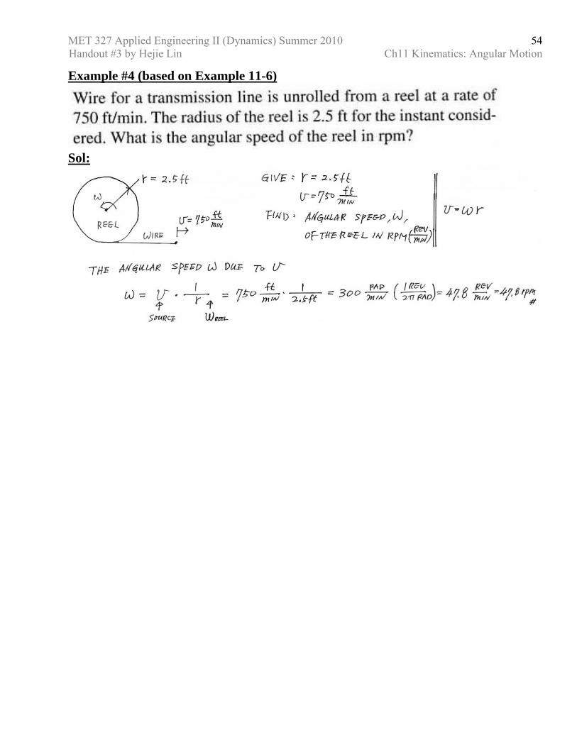
Example #4 (based on Example 11-6)
Sol:
MET 327 Applied Engineering II (Dynamics) Summer 2010 Handout #3 by Hejie Lin Ch11 Kinematics: Angular Motion
55
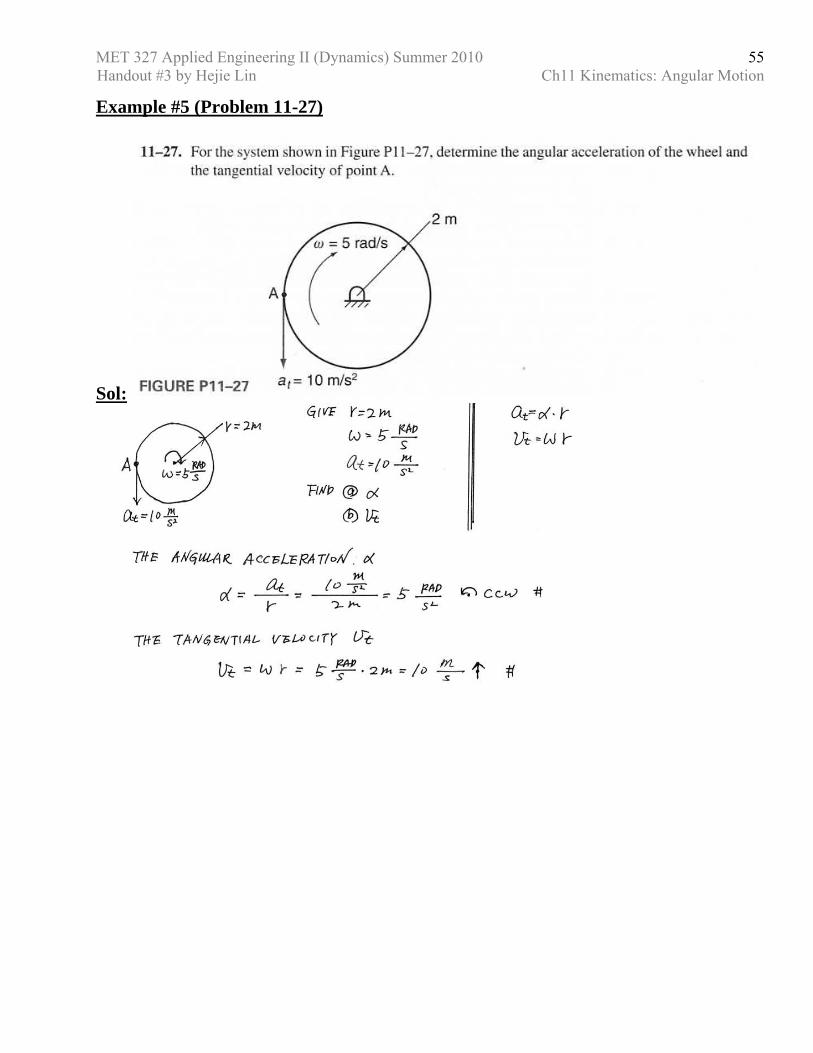
Example #5 (Problem 11-27)
Sol:
MET 327 Applied Engineering II (Dynamics) Summer 2010 Handout #3 by Hejie Lin Ch11 Kinematics: Angular Motion
56
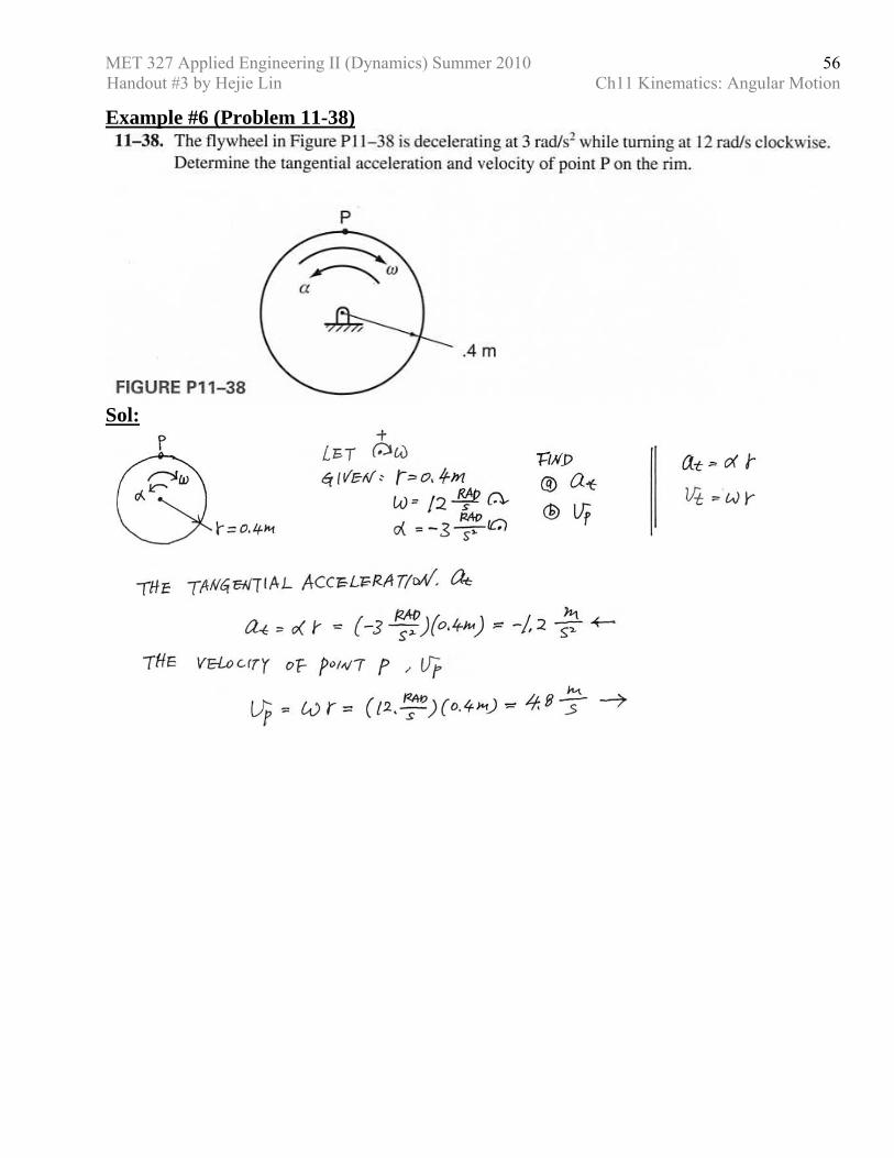
Example #6 (Problem 11-38)
Sol:
MET 327 Applied Engineering II (Dynamics) Summer 2010 Handout #3 by Hejie Lin Ch11 Kinematics: Angular Motion
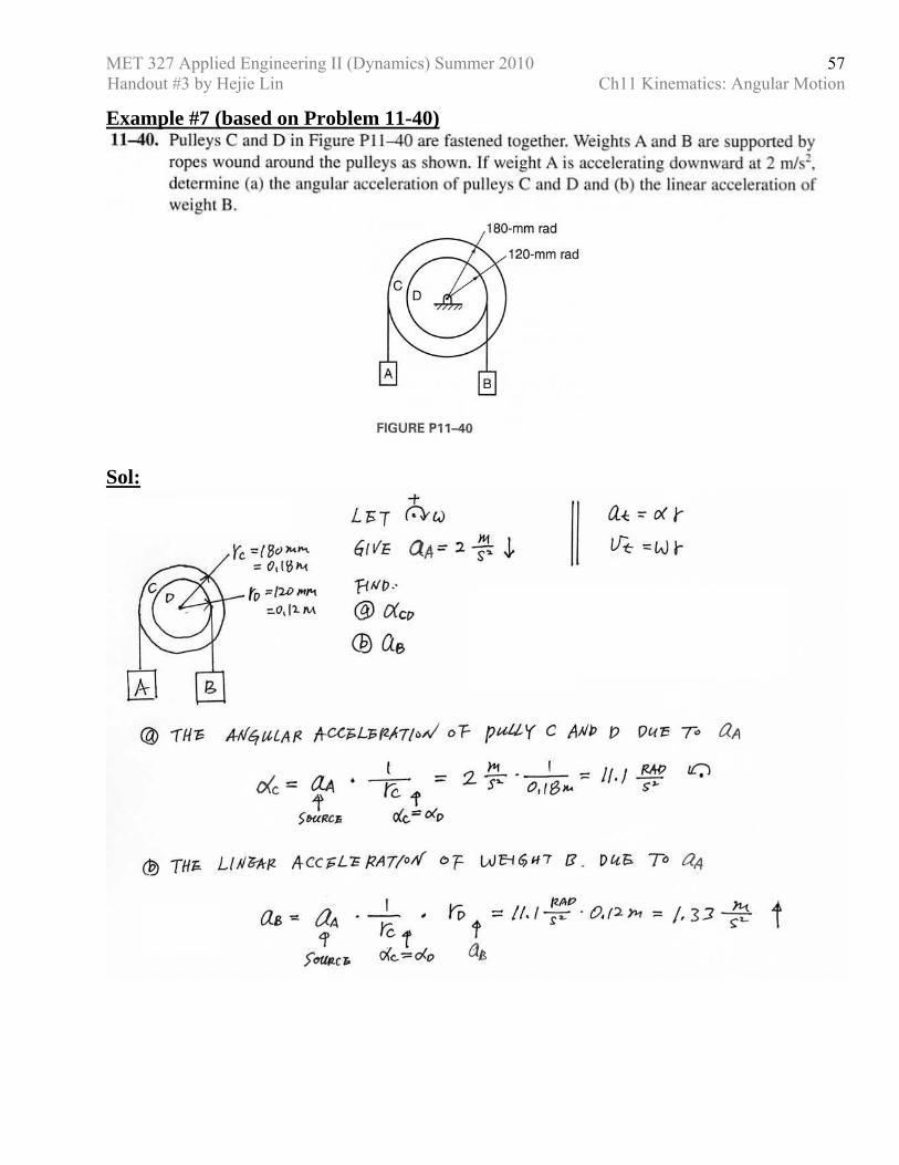
57
Example #7 (based on Problem 11-40)
Sol:
MET 327 Applied Engineering II (Dynamics) Summer 2010 Handout #3 by Hejie Lin Ch11 Kinematics: Angular Motion
58
10-7 Normal and Tangential Acceleration (Page 374) • Tangential acceleration ta is due to the change of magnitude of it linear velocity v
and angular velocity ω values. The direction of tangential acceleration is tangential to the arc of the travel and is therefore perpendicular to the radius.
• Normal acceleration na is due to the change in direction of velocityv . The direction of normal acceleration is normal to the arc of the travel and is therefore parallel to the radius.
• t
∆∆
≡van
• A wheel with radius r turns at constant speed v will have a normal acceleration na as
2
rvan ≡
MET 327 Applied Engineering II (Dynamics) Summer 2010 Handout #3 by Hejie Lin Ch11 Kinematics: Angular Motion
59
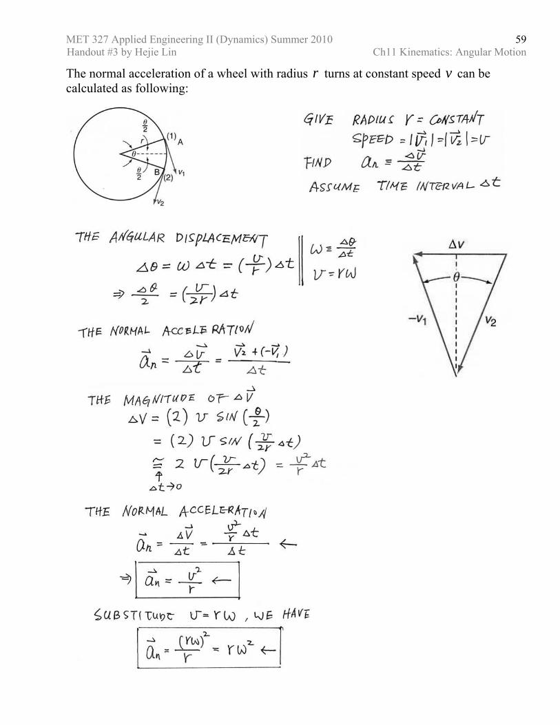
The normal acceleration of a wheel with radius r turns at constant speed v can be calculated as following:
MET 327 Applied Engineering II (Dynamics) Summer 2010 Handout #3 by Hejie Lin Ch11 Kinematics: Angular Motion
60
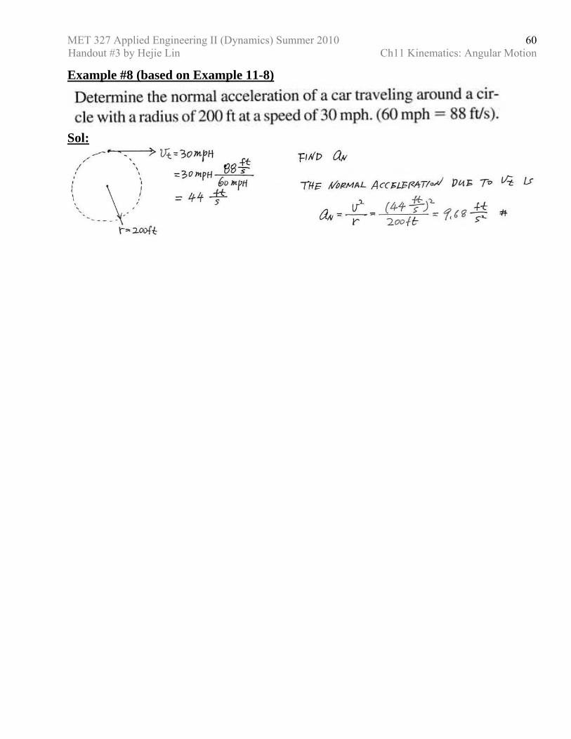
Example #8 (based on Example 11-8)
Sol:
MET 327 Applied Engineering II (Dynamics) Summer 2010 Handout #3 by Hejie Lin Ch11 Kinematics: Angular Motion
61
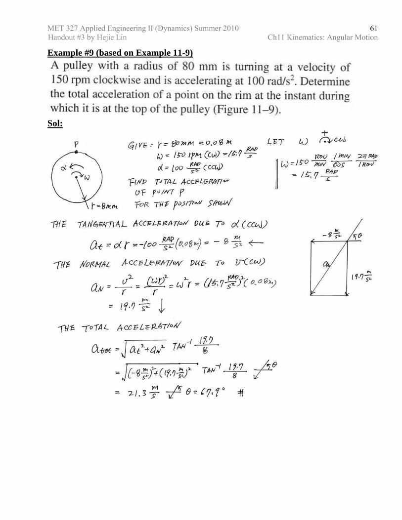
Example #9 (based on Example 11-9)
Sol:
MET 327 Applied Engineering II (Dynamics) Summer 2010 Handout #3 by Hejie Lin Ch11 Kinematics: Angular Motion
62
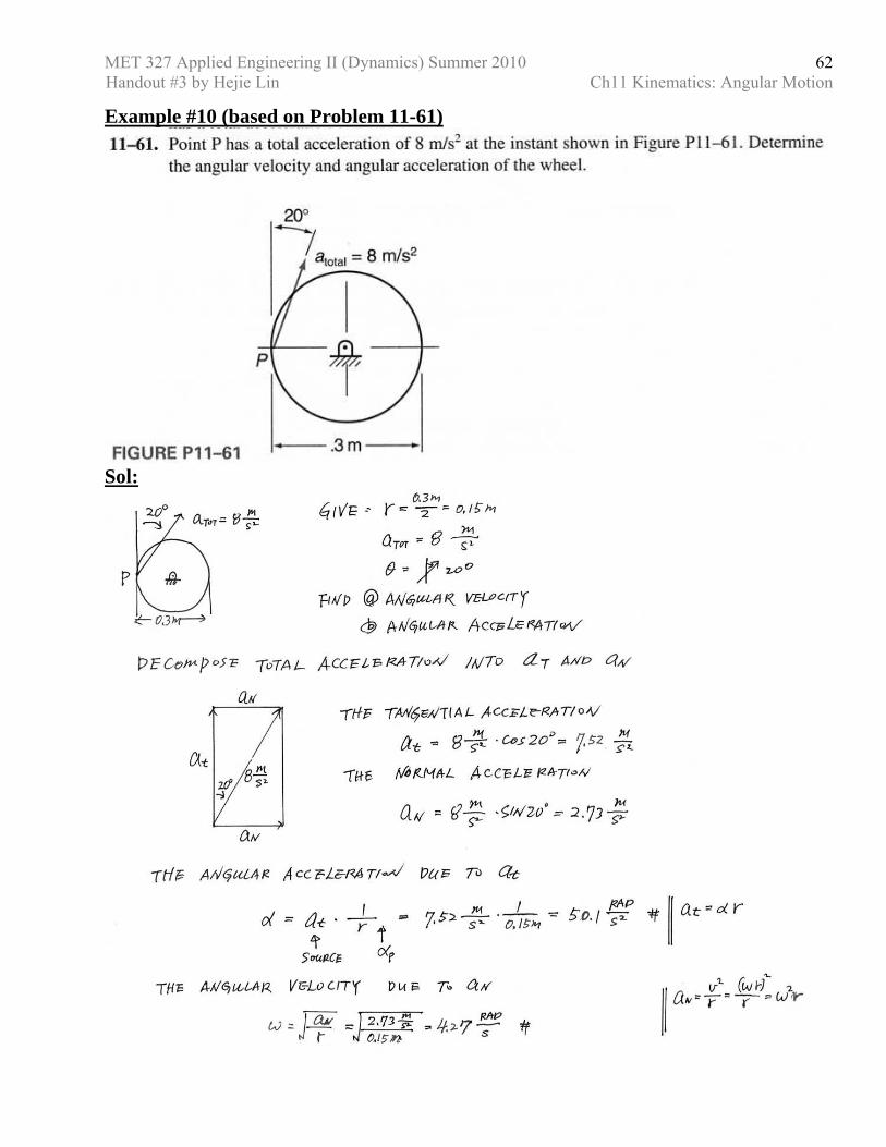
Example #10 (based on Problem 11-61)
Sol:
MET 327 Applied Engineering II (Dynamics) Summer 2010 Handout #3 by Hejie Lin Ch11 Kinematics: Angular Motion
63
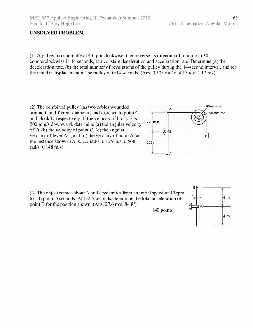
UNSOLVED PROBLEM (1) A pulley turns initially at 40 rpm clockwise, then reverse its direction of rotation to 30 counterclockwise in 14 seconds, at a constant deceleration and acceleration rate. Determine (a) the deceleration rate, (b) the total number of revolutions of the pulley during the 14-second interval, and (c) the angular displacement of the pulley at t=14 seconds. (Ans. 0.523 rad/s², 4.17 rev, 1.17 rev) (2) The combined pulley has two cables wounded around it at different diameters and fastened to point C and block E, respectively. If the velocity of block E is 200 mm/s downward, determine (a) the angular velocity of D, (b) the velocity of point C, (c) the angular velocity of lever AC, and (d) the velocity of point A, at the instance shown. (Ans. 2.5 rad/s, 0.125 m/s, 0.568 rad/s, 0.148 m/s) (3) The object rotates about A and decelerates from an initial speed of 40 rpm to 10 rpm in 5 seconds. At t=2.5 seconds, determine the total acceleration of point B for the position shown. (Ans. 27.6 m/s, 84.8º) [40 points]
MET 327 Applied Engineering II (Dynamics) Summer 2010 Handout #4 by Hejie Lin Ch13 Kinetics
64
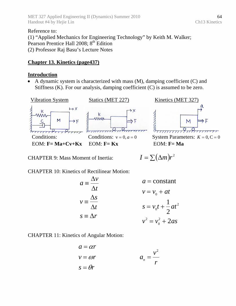
Reference to: (1) “Applied Mechanics for Engineering Technology” by Keith M. Walker; Pearson Prentice Hall 2008; 8th Edition (2) Professor Raj Basu’s Lecture Notes Chapter 13. Kinetics (page437) Introduction • A dynamic system is characterized with mass (M), damping coefficient (C) and
Stiffness (K). For our analysis, damping coefficient (C) is assumed to be zero. Vibration System Statics (MET 227) Kinetics (MET 327)
Conditions: Conditions: 0 0,v == a System Parameters: 0C ,0 ==K EOM: F= Ma+Cv+Kx EOM: F= Kx EOM: F= Ma CHAPTER 9: Mass Moment of Inertia: ( )∑ ∆= 2rmI CHAPTER 10: Kinetics of Rectilinear Motion:
rstsv
tva
∆≡∆∆
≡
∆∆
≡
asvv
attvs
atvva
221
constant
20
2
20
0
+=
+=
+==
CHAPTER 11: Kinetics of Angular Motion:
rsrvra
θωα
===
rvan
2
=
MET 327 Applied Engineering II (Dynamics) Summer 2010 Handout #4 by Hejie Lin Ch13 Kinetics
65
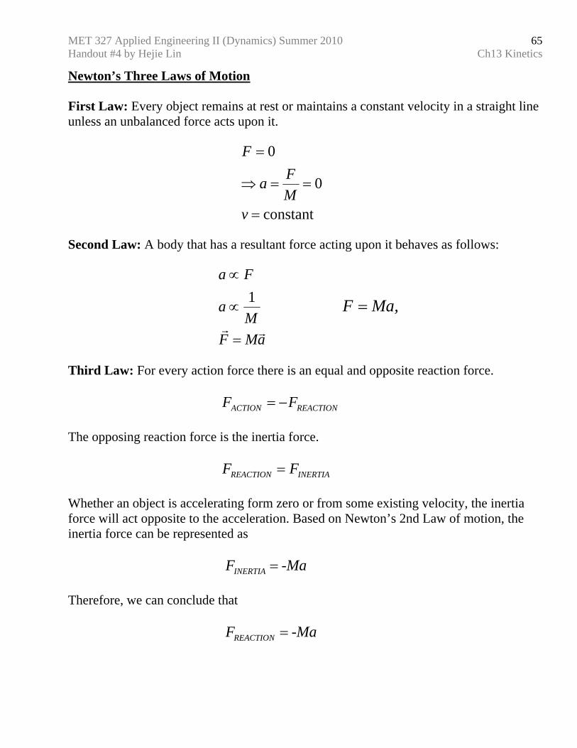
Newton’s Three Laws of Motion First Law: Every object remains at rest or maintains a constant velocity in a straight line unless an unbalanced force acts upon it.
constant
0
0
=
==⇒
=
vMFa
F
Second Law: A body that has a resultant force acting upon it behaves as follows:
aMFM
a
Fa
rr=
∝
∝1
Ma,F =
Third Law: For every action force there is an equal and opposite reaction force. REACTIONACTION FF −= The opposing reaction force is the inertia force. INERTIAREACTION FF = Whether an object is accelerating form zero or from some existing velocity, the inertia force will act opposite to the acceleration. Based on Newton’s 2nd Law of motion, the inertia force can be represented as -MaFINERTIA = Therefore, we can conclude that -MaFREACTION =
MET 327 Applied Engineering II (Dynamics) Summer 2010 Handout #4 by Hejie Lin Ch13 Kinetics
66
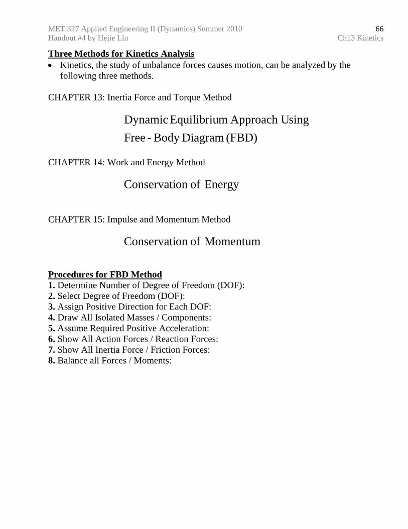
Three Methods for Kinetics Analysis • Kinetics, the study of unbalance forces causes motion, can be analyzed by the
following three methods. CHAPTER 13: Inertia Force and Torque Method
(FBD) DiagramBody -Free
singApproach UmEquilibriuDynamic
CHAPTER 14: Work and Energy Method Energyofon Conservati CHAPTER 15: Impulse and Momentum Method Momentumofon Conservati Procedures for FBD Method 1. Determine Number of Degree of Freedom (DOF): 2. Select Degree of Freedom (DOF): 3. Assign Positive Direction for Each DOF: 4. Draw All Isolated Masses / Components: 5. Assume Required Positive Acceleration: 6. Show All Action Forces / Reaction Forces: 7. Show All Inertia Force / Friction Forces: 8. Balance all Forces / Moments:
MET 327 Applied Engineering II (Dynamics) Summer 2010 Handout #4 by Hejie Lin Ch13 Kinetics
67
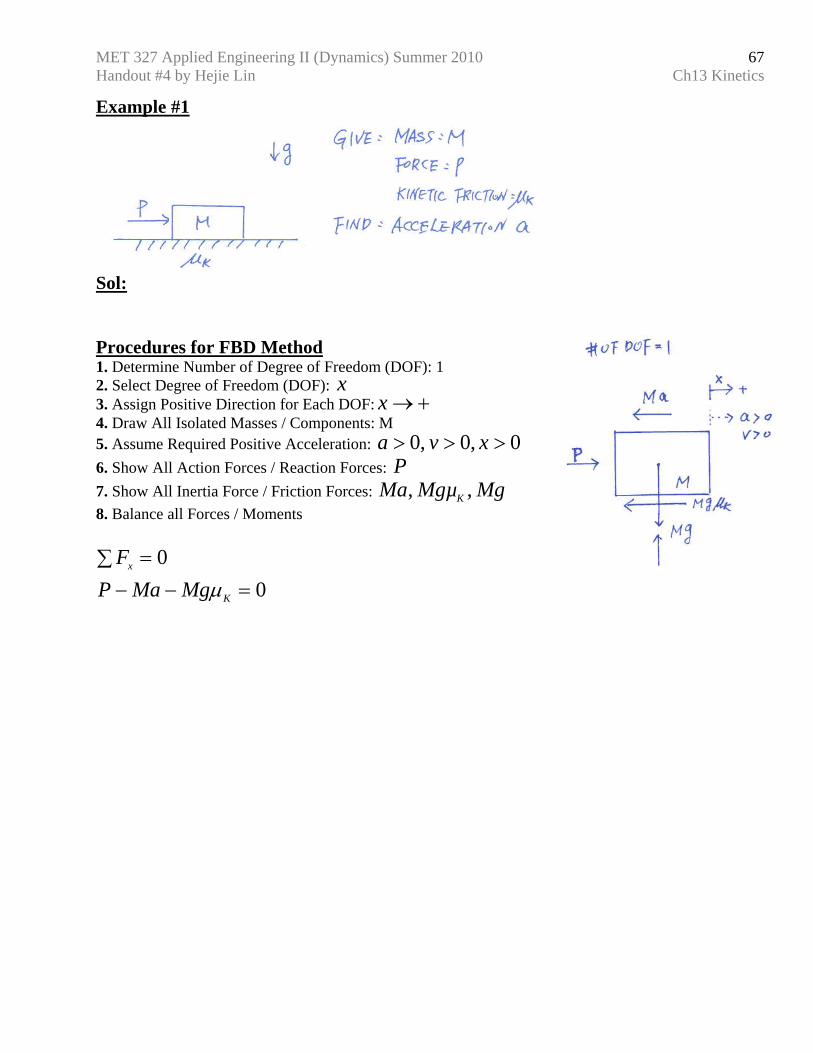
Example #1
Sol: Procedures for FBD Method 1. Determine Number of Degree of Freedom (DOF): 1 2. Select Degree of Freedom (DOF): x 3. Assign Positive Direction for Each DOF: +→x 4. Draw All Isolated Masses / Components: M 5. Assume Required Positive Acceleration: 0,0,0 >>> xva 6. Show All Action Forces / Reaction Forces: P 7. Show All Inertia Force / Friction Forces: MgMgµMa K , , 8. Balance all Forces / Moments
0 0
=−−∑ =
K
x
MgMaPF
µ
MET 327 Applied Engineering II (Dynamics) Summer 2010 Handout #4 by Hejie Lin Ch13 Kinetics
68
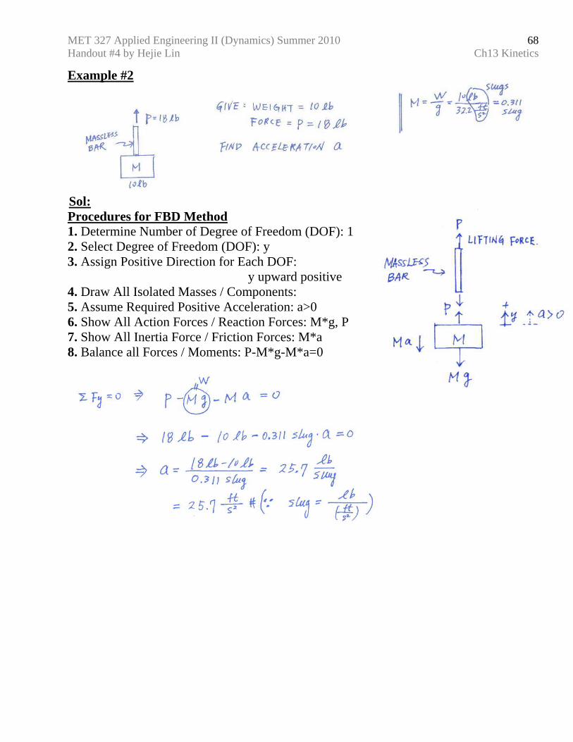
Example #2
Sol: Procedures for FBD Method 1. Determine Number of Degree of Freedom (DOF): 1 2. Select Degree of Freedom (DOF): y 3. Assign Positive Direction for Each DOF: y upward positive 4. Draw All Isolated Masses / Components: 5. Assume Required Positive Acceleration: a>0 6. Show All Action Forces / Reaction Forces: M*g, P 7. Show All Inertia Force / Friction Forces: M*a 8. Balance all Forces / Moments: P-M*g-M*a=0
MET 327 Applied Engineering II (Dynamics) Summer 2010 Handout #4 by Hejie Lin Ch13 Kinetics
69
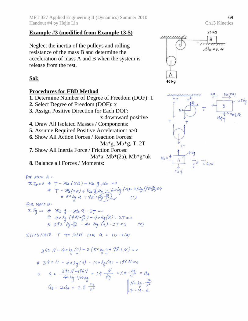
Example #3 (modified from Example 13-5) Neglect the inertia of the pulleys and rolling resistance of the mass B and determine the acceleration of mass A and B when the system is release from the rest. Sol: Procedures for FBD Method 1. Determine Number of Degree of Freedom (DOF): 1 2. Select Degree of Freedom (DOF): x 3. Assign Positive Direction for Each DOF: x downward positive 4. Draw All Isolated Masses / Components: 5. Assume Required Positive Acceleration: a>0 6. Show All Action Forces / Reaction Forces: Ma*g, Mb*g, T, 2T 7. Show All Inertia Force / Friction Forces: Ma*a, Mb*(2a), Mb*g*uk 8. Balance all Forces / Moments:
MET 327 Applied Engineering II (Dynamics) Summer 2010 Handout #4 by Hejie Lin Ch13 Kinetics
70
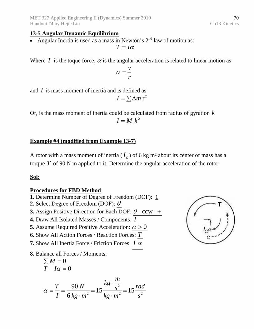
13-5 Angular Dynamic Equilibrium • Angular Inertia is used as a mass in Newton’s 2nd law of motion as: αIT = Where T is the toque force, α is the angular acceleration is related to linear motion as
rv
=α
and I is mass moment of inertia and is defined as 2r ∑∆= mI Or, is the mass moment of inertia could be calculated from radius of gyration k 2kMI = Example #4 (modified from Example 13-7) A rotor with a mass moment of inertia ( CI ) of 6 kg m² about its center of mass has a torque T of 90 N m applied to it. Determine the angular acceleration of the rotor. Sol: Procedures for FBD Method 1. Determine Number of Degree of Freedom (DOF): 1 2. Select Degree of Freedom (DOF): θ 3. Assign Positive Direction for Each DOF: + ccw θ 4. Draw All Isolated Masses / Components: I 5. Assume Required Positive Acceleration: 0>α 6. Show All Action Forces / Reaction Forces: T 7. Show All Inertia Force / Friction Forces: αI
8. Balance all Forces / Moments: ∑ = 0M
22
2
2 1515 6
90
0
srad
mkgsmkg
mkgN
IT
IT
=⋅
⋅=
⋅==
=−
α
α
MET 327 Applied Engineering II (Dynamics) Summer 2010 Handout #4 by Hejie Lin Ch13 Kinetics
71
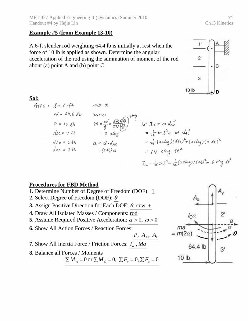
Example #5 (from Example 13-10) A 6-ft slender rod weighting 64.4 lb is initially at rest when the force of 10 lb is applied as shown. Determine the angular acceleration of the rod using the summation of moment of the rod about (a) point A and (b) point C. Sol:
Procedures for FBD Method 1. Determine Number of Degree of Freedom (DOF): 1 2. Select Degree of Freedom (DOF): θ 3. Assign Positive Direction for Each DOF: + ccw θ 4. Draw All Isolated Masses / Components: rod 5. Assume Required Positive Acceleration: 0 ,0 >> ωα 6. Show All Action Forces / Reaction Forces: YX AAP , , 7. Show All Inertia Force / Friction Forces: MaI , α 8. Balance all Forces / Moments 0 ,0 ,0or 0 =∑=∑ ∑∑ == xyCA FFMM
MET 327 Applied Engineering II (Dynamics) Summer 2010 Handout #4 by Hejie Lin Ch13 Kinetics
72
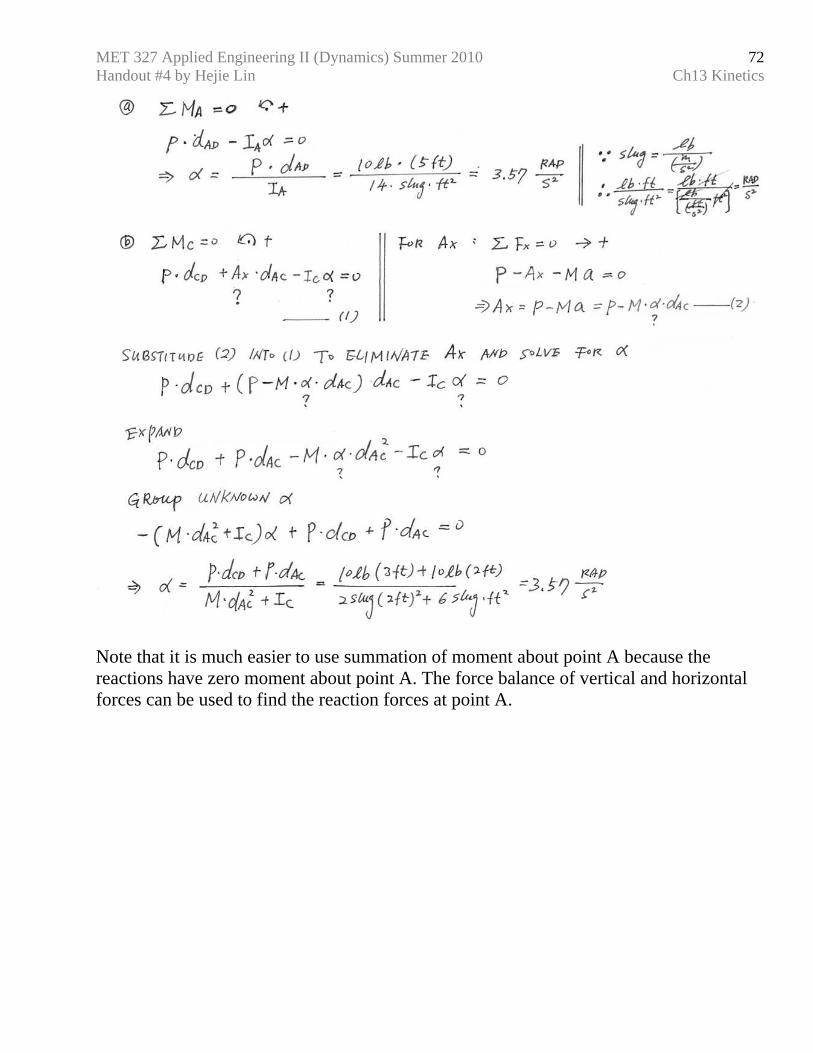
Note that it is much easier to use summation of moment about point A because the reactions have zero moment about point A. The force balance of vertical and horizontal forces can be used to find the reaction forces at point A.
MET 327 Applied Engineering II (Dynamics) Summer 2010 Handout #4 by Hejie Lin Ch13 Kinetics
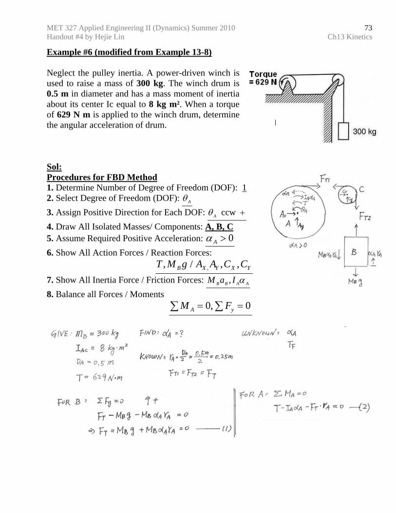
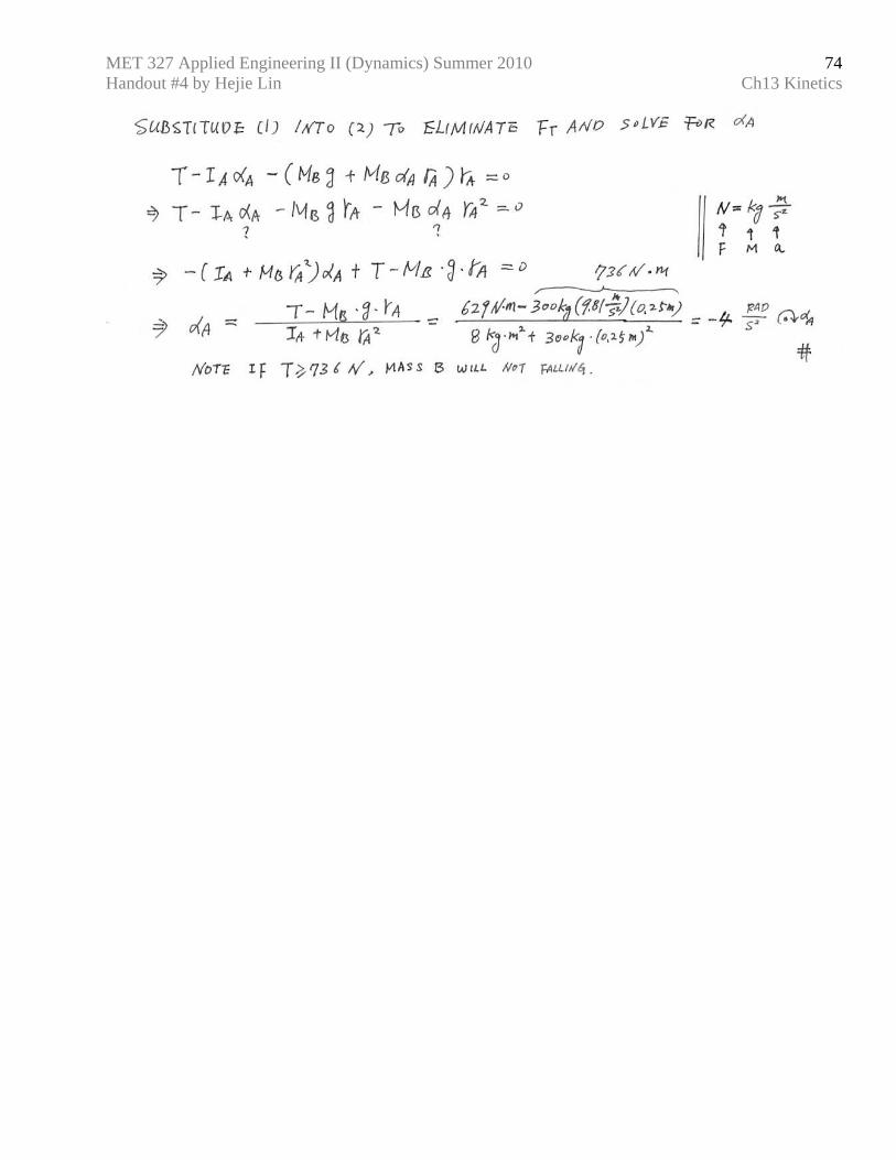
73
Example #6 (modified from Example 13-8) Neglect the pulley inertia. A power-driven winch is used to raise a mass of 300 kg. The winch drum is 0.5 m in diameter and has a mass moment of inertia about its center Ic equal to 8 kg m². When a torque of 629 N m is applied to the winch drum, determine the angular acceleration of drum. Sol: Procedures for FBD Method 1. Determine Number of Degree of Freedom (DOF): 1 2. Select Degree of Freedom (DOF): Aθ 3. Assign Positive Direction for Each DOF: + ccw Aθ 4. Draw All Isolated Masses/ Components: A, B, C 5. Assume Required Positive Acceleration: 0>Aα 6. Show All Action Forces / Reaction Forces: YXYXB CCAAgMT ,, / , ,
7. Show All Inertia Force / Friction Forces: AABB IaM α, 8. Balance all Forces / Moments 0 ,0 ==∑ ∑ yA FM
MET 327 Applied Engineering II (Dynamics) Summer 2010 Handout #4 by Hejie Lin Ch13 Kinetics
74
MET 327 Applied Engineering II (Dynamics) Summer 2010 Handout #4 by Hejie Lin Ch13 Kinetics
75
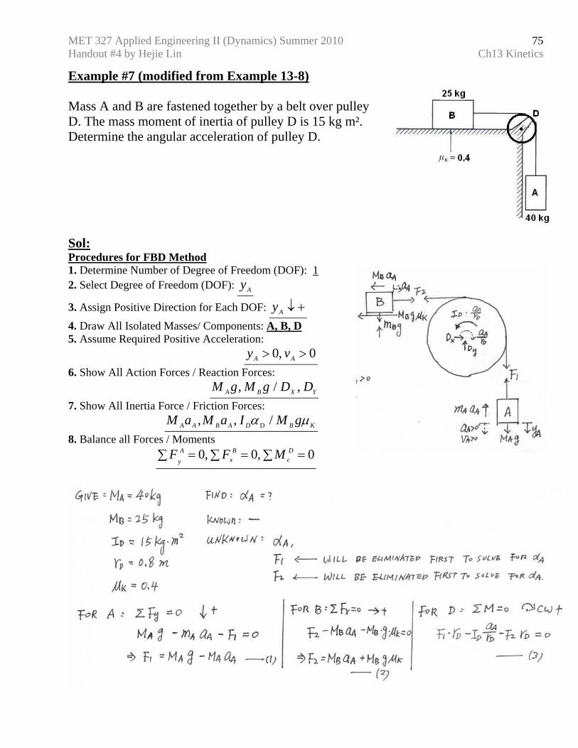
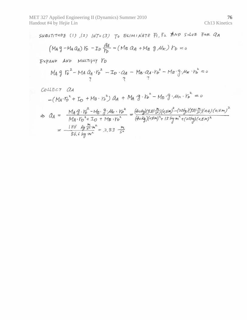
Example #7 (modified from Example 13-8) Mass A and B are fastened together by a belt over pulley D. The mass moment of inertia of pulley D is 15 kg m². Determine the angular acceleration of pulley D. Sol: Procedures for FBD Method 1. Determine Number of Degree of Freedom (DOF): 1 2. Select Degree of Freedom (DOF): Ay
3. Assign Positive Direction for Each DOF: +↓Ay
4. Draw All Isolated Masses/ Components: A, B, D 5. Assume Required Positive Acceleration: 0 ,0 >> AA vy
6. Show All Action Forces / Reaction Forces: YXBA DDgMgM , / ,
7. Show All Inertia Force / Friction Forces: KBDABAA gMIaMaM µα / ,, D
8. Balance all Forces / Moments 0 ,0 ,0 =∑=∑ ∑= D
cB
xA
yMFF
MET 327 Applied Engineering II (Dynamics) Summer 2010 Handout #4 by Hejie Lin Ch13 Kinetics
76
MET 327 Applied Engineering II (Dynamics) Summer 2010 Handout #4 by Hejie Lin Ch13 Kinetics
77
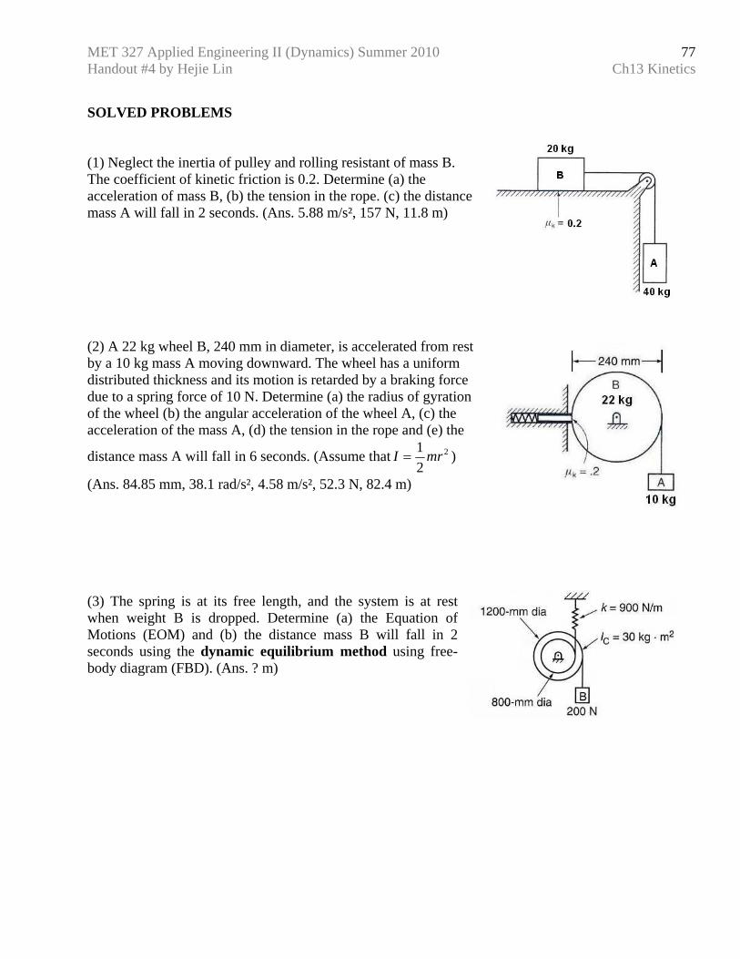
SOLVED PROBLEMS (1) Neglect the inertia of pulley and rolling resistant of mass B. The coefficient of kinetic friction is 0.2. Determine (a) the acceleration of mass B, (b) the tension in the rope. (c) the distance mass A will fall in 2 seconds. (Ans. 5.88 m/s², 157 N, 11.8 m) (2) A 22 kg wheel B, 240 mm in diameter, is accelerated from rest by a 10 kg mass A moving downward. The wheel has a uniform distributed thickness and its motion is retarded by a braking force due to a spring force of 10 N. Determine (a) the radius of gyration of the wheel (b) the angular acceleration of the wheel A, (c) the acceleration of the mass A, (d) the tension in the rope and (e) the
distance mass A will fall in 6 seconds. (Assume that 2
21 mrI = )
(Ans. 84.85 mm, 38.1 rad/s², 4.58 m/s², 52.3 N, 82.4 m) (3) The spring is at its free length, and the system is at rest when weight B is dropped. Determine (a) the Equation of Motions (EOM) and (b) the distance mass B will fall in 2 seconds using the dynamic equilibrium method using free-body diagram (FBD). (Ans. ? m)
MET 327 Applied Engineering II (Dynamics) Summer 2010 Handout #5 by Hejie Lin Chapter 14: Work, Energy, and Power
78
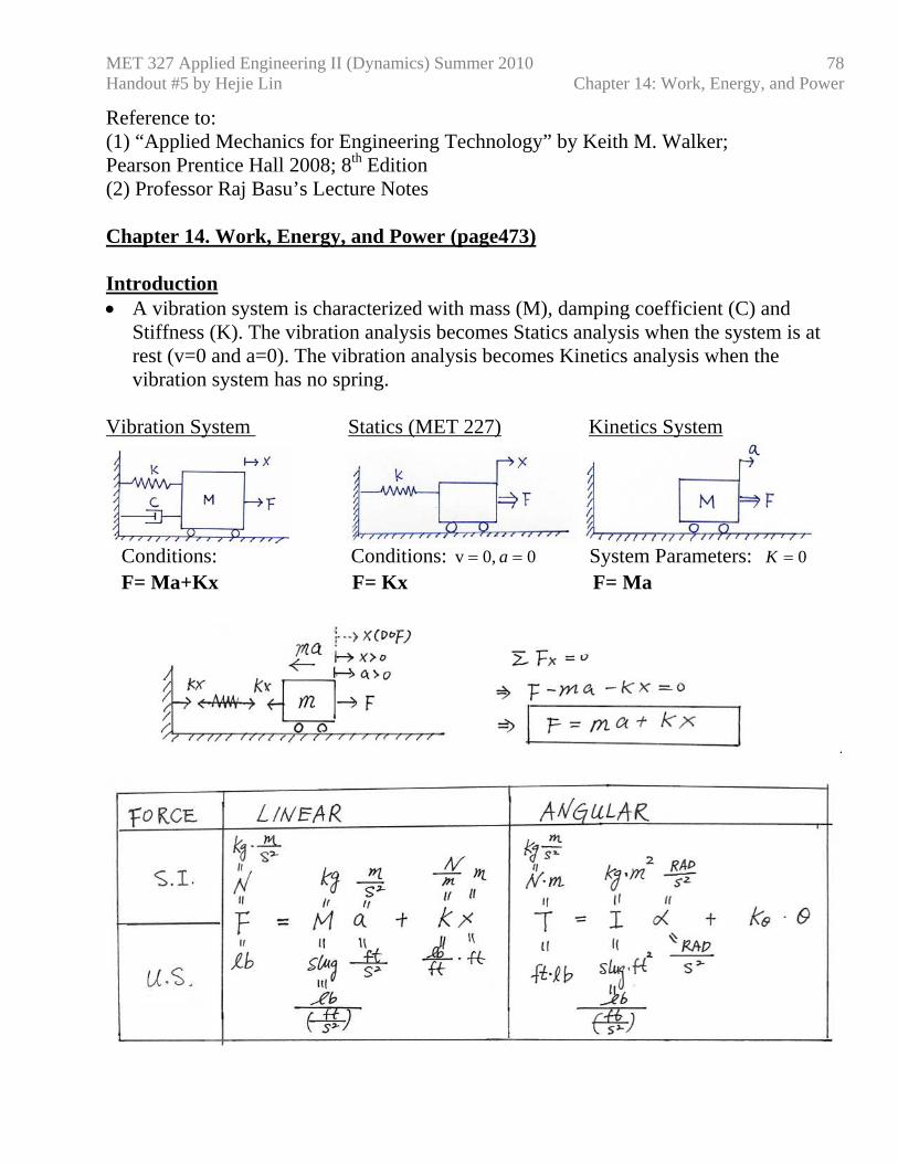
Reference to: (1) “Applied Mechanics for Engineering Technology” by Keith M. Walker; Pearson Prentice Hall 2008; 8th Edition (2) Professor Raj Basu’s Lecture Notes Chapter 14. Work, Energy, and Power (page473) Introduction • A vibration system is characterized with mass (M), damping coefficient (C) and
Stiffness (K). The vibration analysis becomes Statics analysis when the system is at rest (v=0 and a=0). The vibration analysis becomes Kinetics analysis when the vibration system has no spring.
Vibration System Statics (MET 227) Kinetics System
Conditions: Conditions: 0 0,v == a System Parameters: 0=K F= Ma+Kx F= Kx F= Ma
MET 327 Applied Engineering II (Dynamics) Summer 2010 Handout #5 by Hejie Lin Chapter 14: Work, Energy, and Power
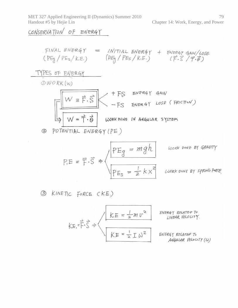
79
MET 327 Applied Engineering II (Dynamics) Summer 2010 Handout #5 by Hejie Lin Chapter 14: Work, Energy, and Power
80
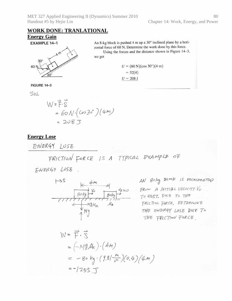
WORK DONE: TRANLATIONAL Energy Gain
Energy Lose
MET 327 Applied Engineering II (Dynamics) Summer 2010 Handout #5 by Hejie Lin Chapter 14: Work, Energy, and Power
81
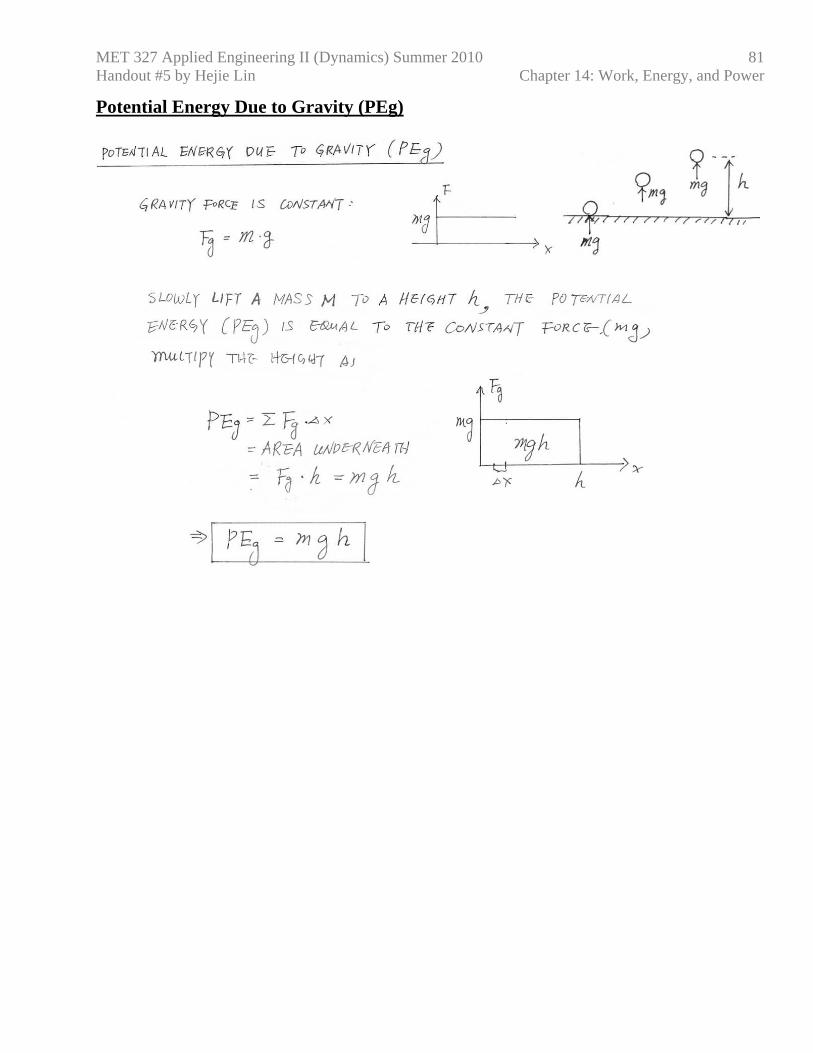
Potential Energy Due to Gravity (PEg)
MET 327 Applied Engineering II (Dynamics) Summer 2010 Handout #5 by Hejie Lin Chapter 14: Work, Energy, and Power
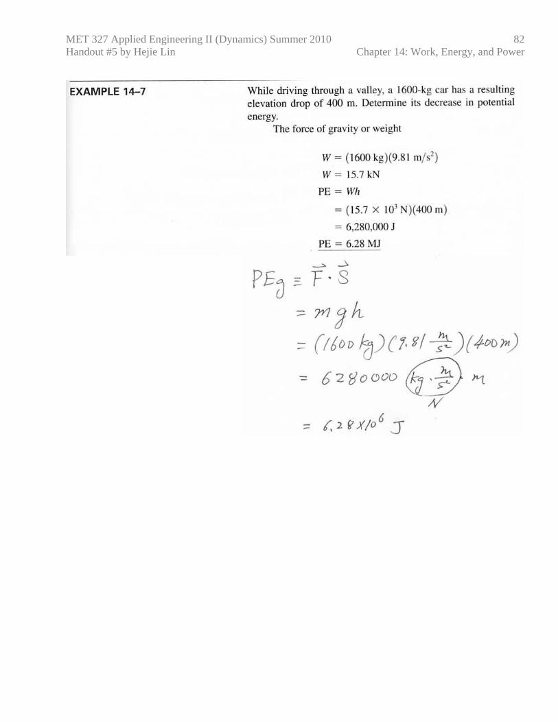
82
MET 327 Applied Engineering II (Dynamics) Summer 2010 Handout #5 by Hejie Lin Chapter 14: Work, Energy, and Power
83
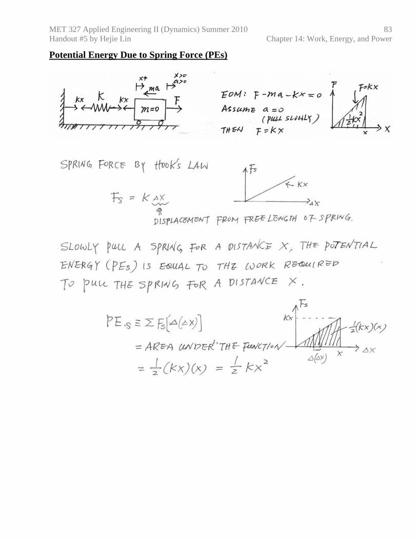
Potential Energy Due to Spring Force (PEs)
MET 327 Applied Engineering II (Dynamics) Summer 2010 Handout #5 by Hejie Lin Chapter 14: Work, Energy, and Power
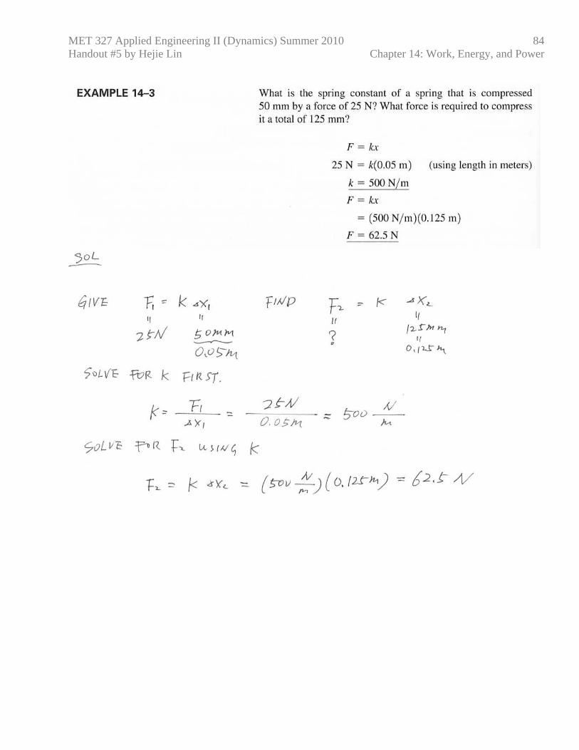
84
MET 327 Applied Engineering II (Dynamics) Summer 2010 Handout #5 by Hejie Lin Chapter 14: Work, Energy, and Power
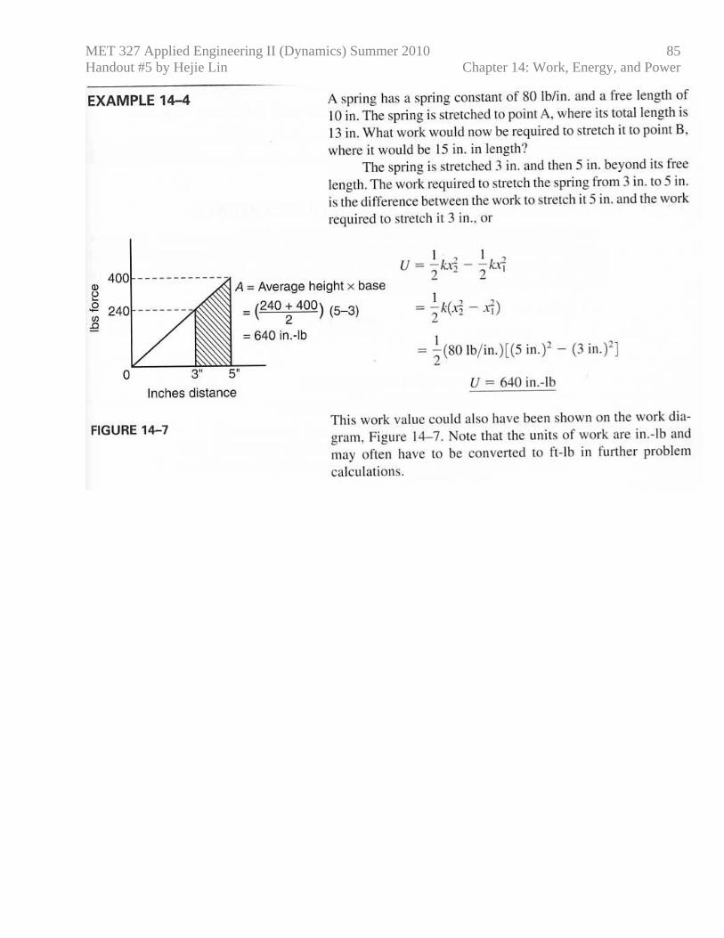
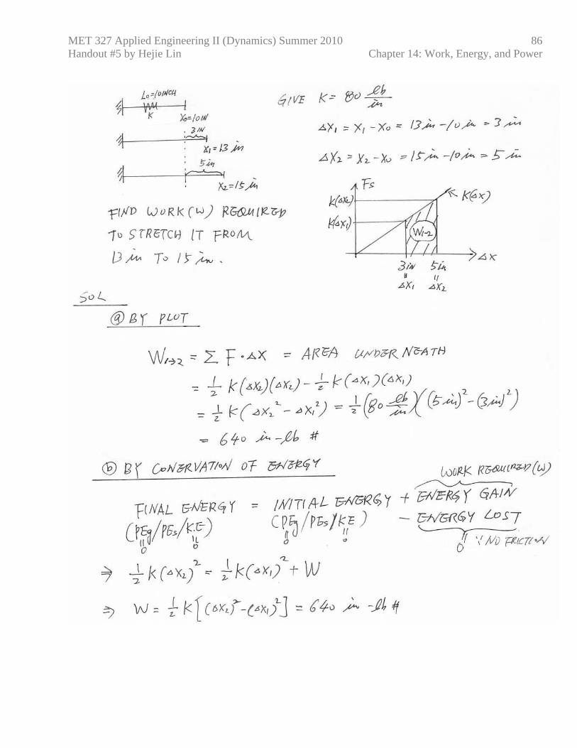
85
MET 327 Applied Engineering II (Dynamics) Summer 2010 Handout #5 by Hejie Lin Chapter 14: Work, Energy, and Power
86
MET 327 Applied Engineering II (Dynamics) Summer 2010 Handout #5 by Hejie Lin Chapter 14: Work, Energy, and Power
87
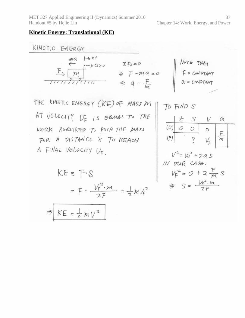
Kinetic Energy: Translational (KE)
MET 327 Applied Engineering II (Dynamics) Summer 2010 Handout #5 by Hejie Lin Chapter 14: Work, Energy, and Power
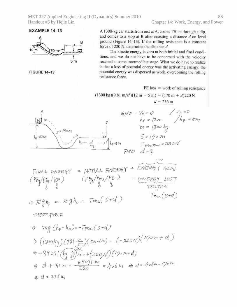
88
MET 327 Applied Engineering II (Dynamics) Summer 2010 Handout #5 by Hejie Lin Chapter 14: Work, Energy, and Power
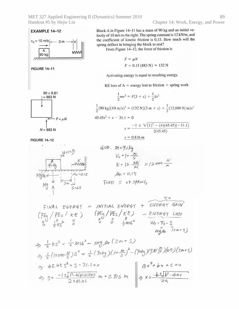
89
MET 327 Applied Engineering II (Dynamics) Summer 2010 Handout #5 by Hejie Lin Chapter 14: Work, Energy, and Power
90
WORK DONE: ANGULAR
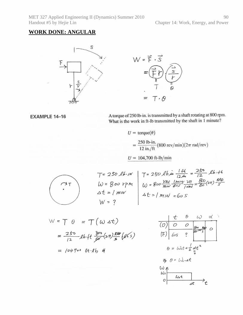
MET 327 Applied Engineering II (Dynamics) Summer 2010 Handout #5 by Hejie Lin Chapter 14: Work, Energy, and Power
91
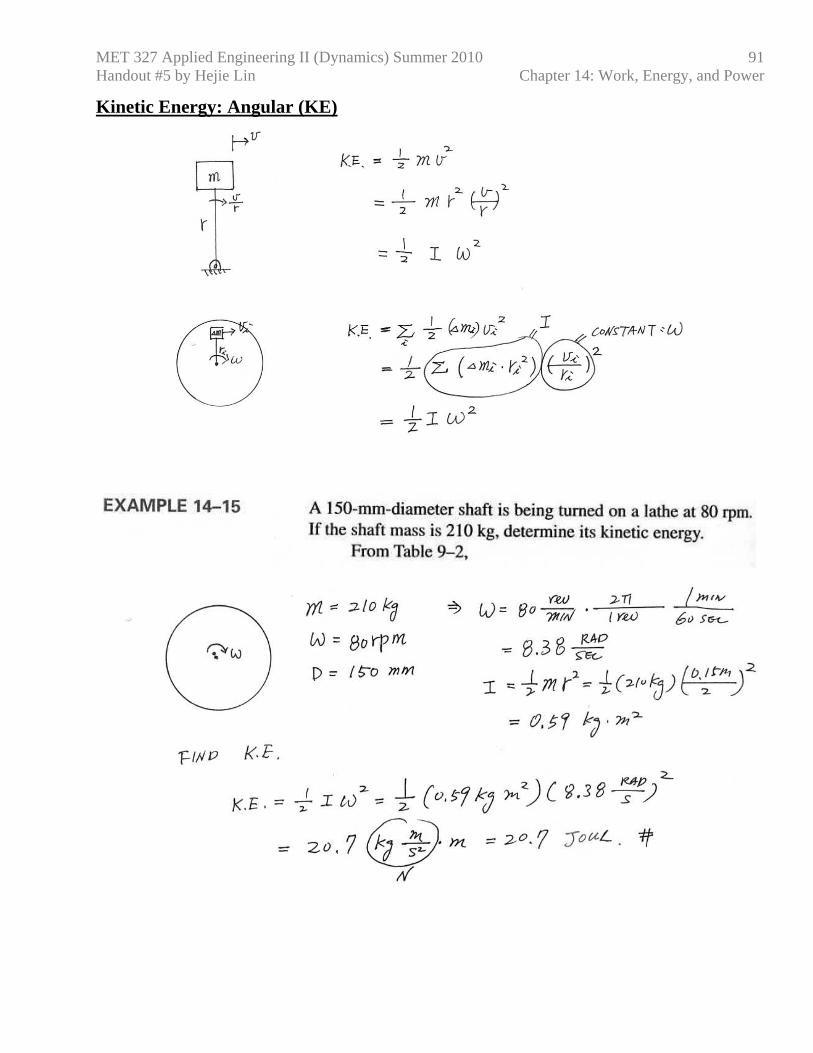
Kinetic Energy: Angular (KE)
MET 327 Applied Engineering II (Dynamics) Summer 2010 Handout #5 by Hejie Lin Chapter 14: Work, Energy, and Power
92
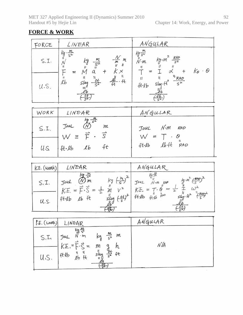
FORCE & WORK
MET 327 Applied Engineering II (Dynamics) Summer 2010 Handout #5 by Hejie Lin Chapter 14: Work, Energy, and Power
93
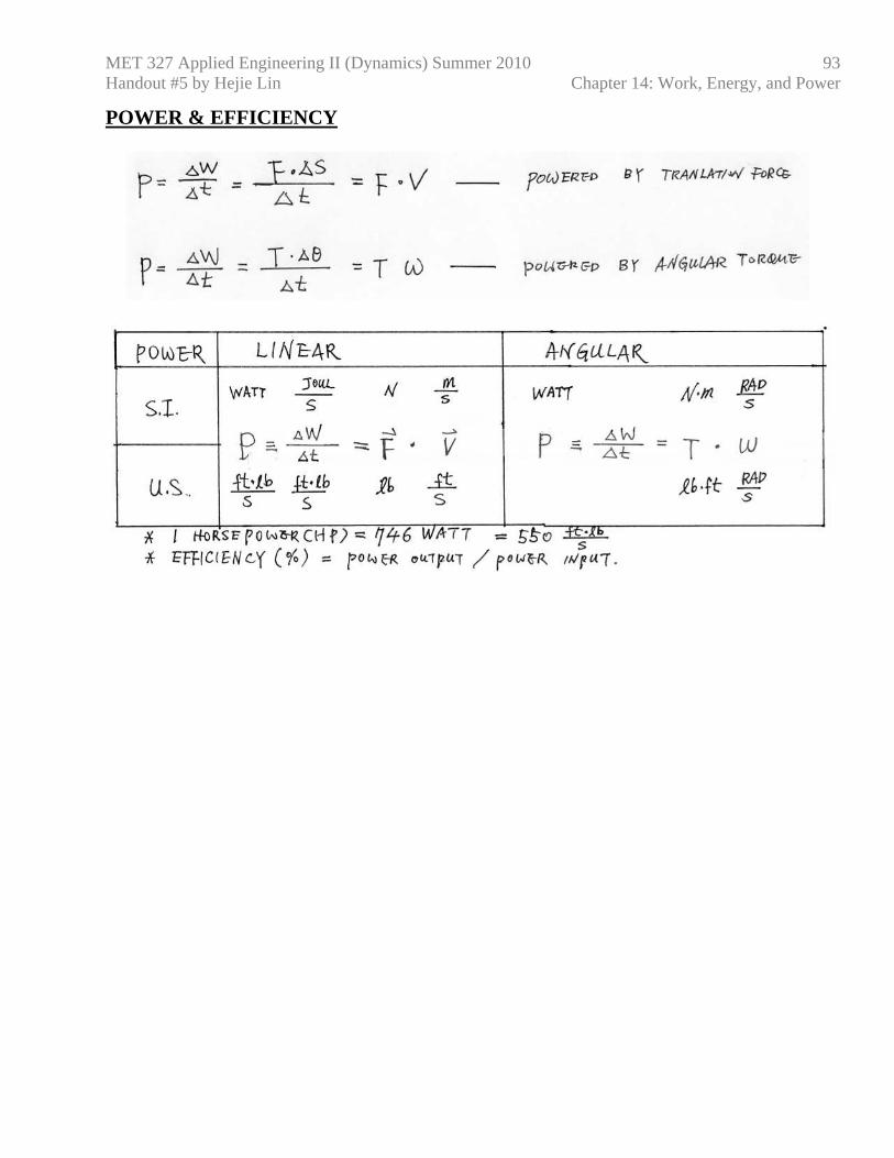
POWER & EFFICIENCY
MET 327 Applied Engineering II (Dynamics) Summer 2010 Handout #5 by Hejie Lin Chapter 14: Work, Energy, and Power
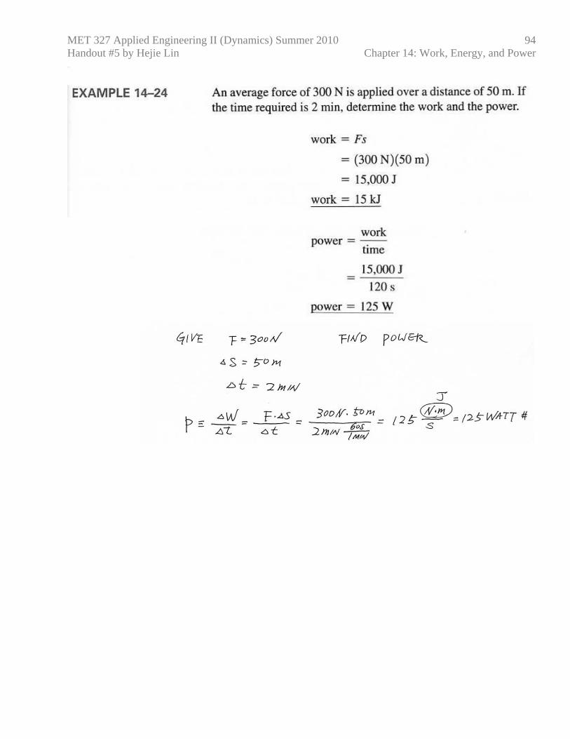
94
MET 327 Applied Engineering II (Dynamics) Summer 2010 Handout #5 by Hejie Lin Chapter 14: Work, Energy, and Power
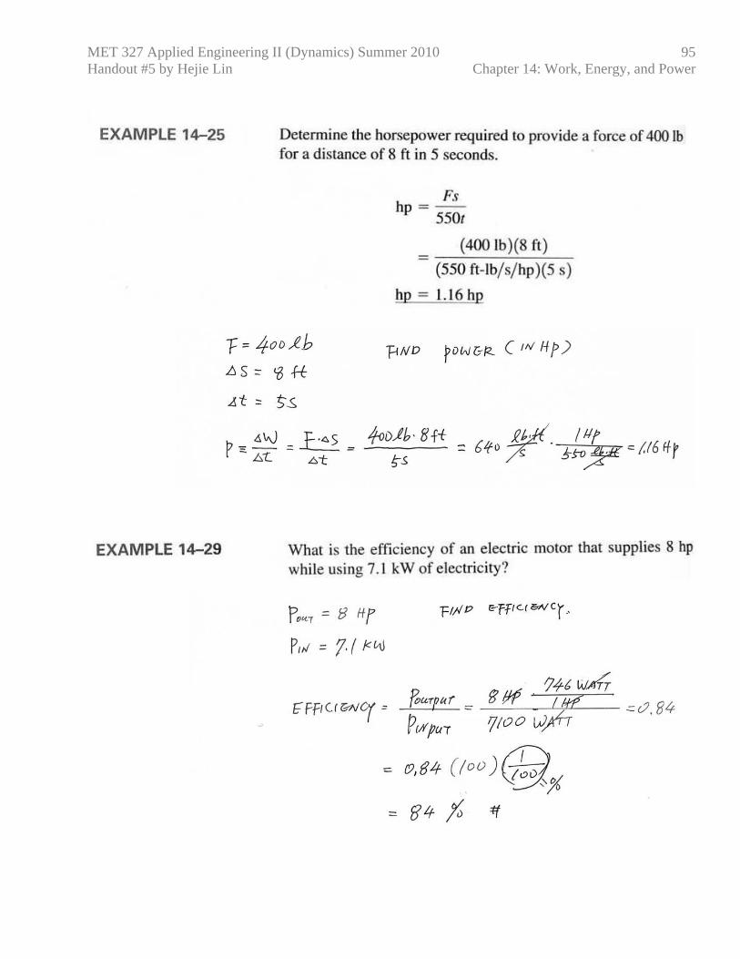
95
MET 327 Applied Engineering II (Dynamics) Summer 2010 Handout #5 by Hejie Lin Chapter 14: Work, Energy, and Power
96
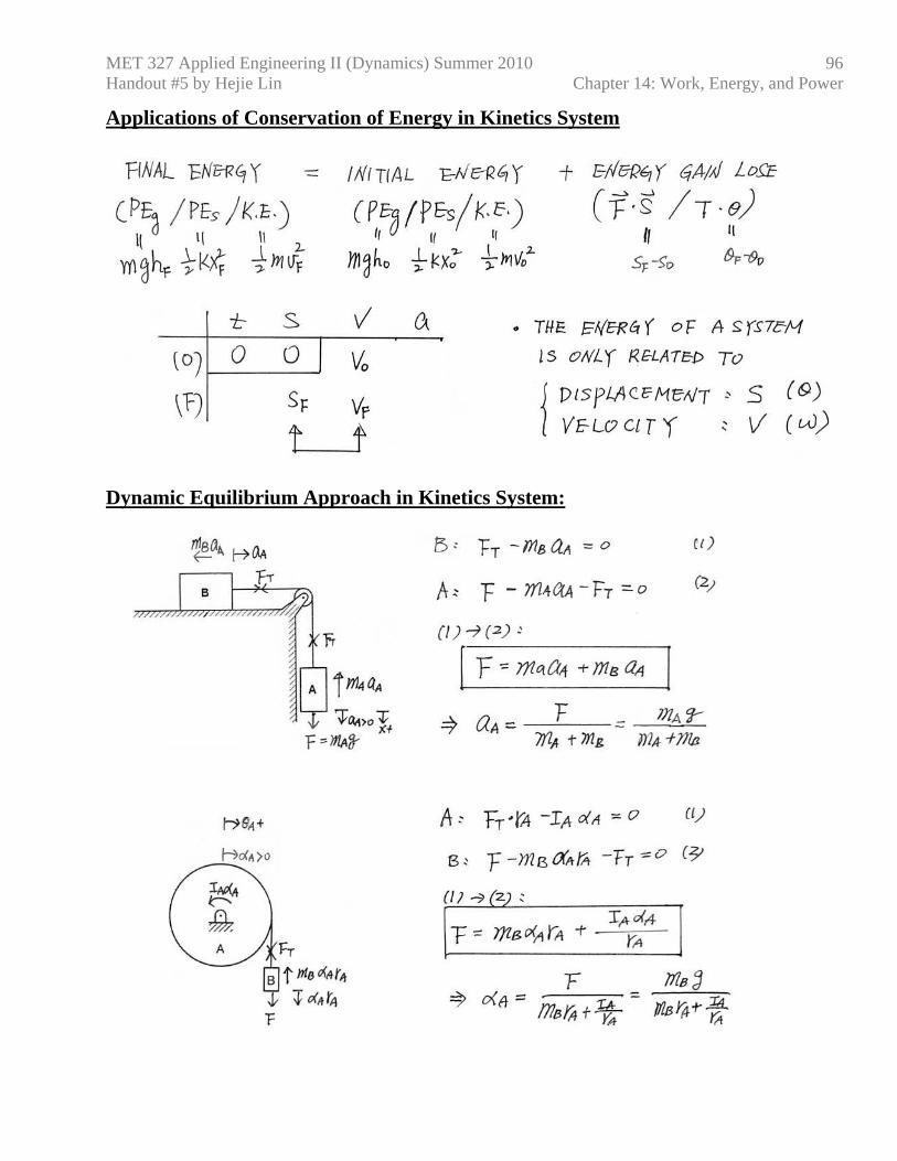
Applications of Conservation of Energy in Kinetics System
Dynamic Equilibrium Approach in Kinetics System:
MET 327 Applied Engineering II (Dynamics) Summer 2010 Handout #5 by Hejie Lin Chapter 14: Work, Energy, and Power
97
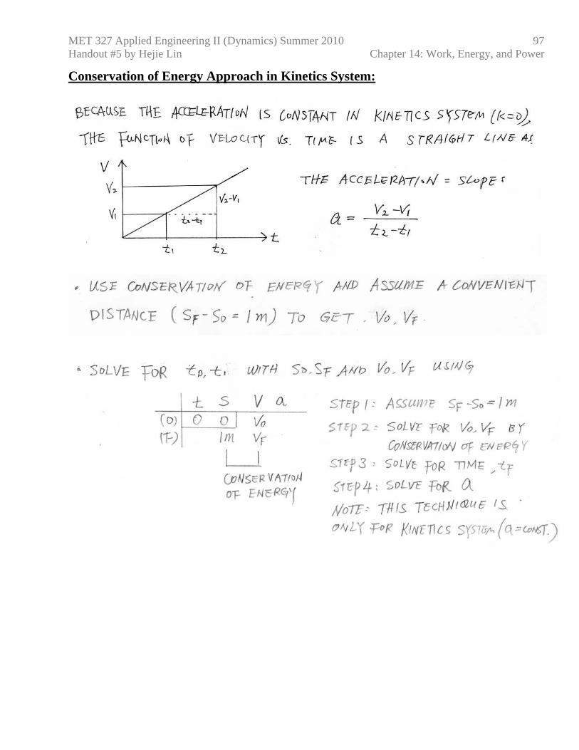
Conservation of Energy Approach in Kinetics System:
MET 327 Applied Engineering II (Dynamics) Summer 2010 Handout #5 by Hejie Lin Chapter 14: Work, Energy, and Power
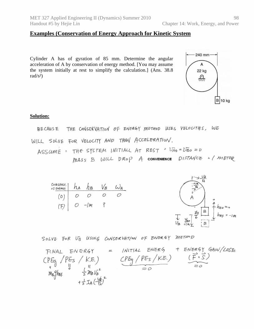
98
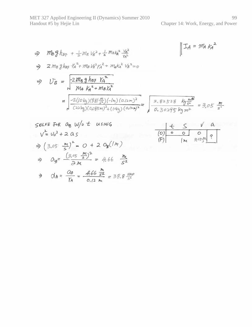
Examples (Conservation of Energy Approach for Kinetic System Cylinder A has of gyration of 85 mm. Determine the angular acceleration of A by conservation of energy method. [You may assume the system initially at rest to simplify the calculation.] (Ans. 38.8 rad/s²) Solution:
MET 327 Applied Engineering II (Dynamics) Summer 2010 Handout #5 by Hejie Lin Chapter 14: Work, Energy, and Power
99
MET 327 Applied Engineering II (Dynamics) Summer 2010 Handout #5 by Hejie Lin Chapter 14: Work, Energy, and Power
100
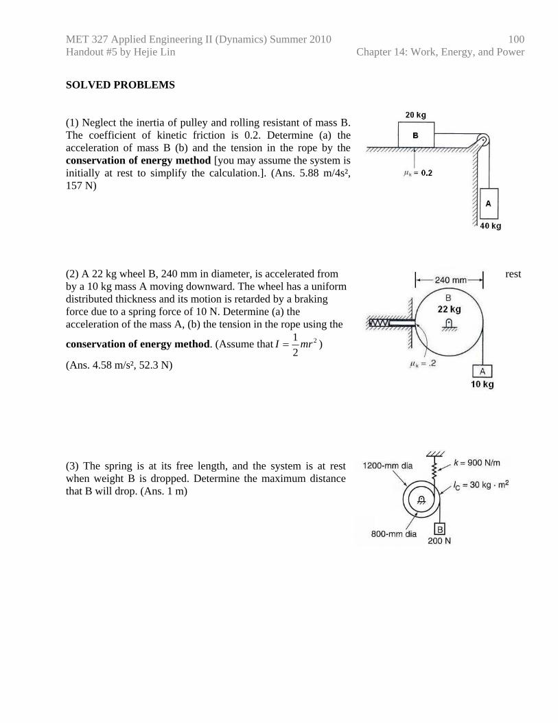
SOLVED PROBLEMS (1) Neglect the inertia of pulley and rolling resistant of mass B. The coefficient of kinetic friction is 0.2. Determine (a) the acceleration of mass B (b) and the tension in the rope by the conservation of energy method [you may assume the system is initially at rest to simplify the calculation.]. (Ans. 5.88 m/4s², 157 N) (2) A 22 kg wheel B, 240 mm in diameter, is accelerated from rest by a 10 kg mass A moving downward. The wheel has a uniform distributed thickness and its motion is retarded by a braking force due to a spring force of 10 N. Determine (a) the acceleration of the mass A, (b) the tension in the rope using the
conservation of energy method. (Assume that 2
21 mrI = )
(Ans. 4.58 m/s², 52.3 N) (3) The spring is at its free length, and the system is at rest when weight B is dropped. Determine the maximum distance that B will drop. (Ans. 1 m)
MET 327 Applied Engineering II (Dynamics) Summer 2010 Handout #6 (8/12) by Hejie Lin Chapter 15: Impulse and Momentum
101
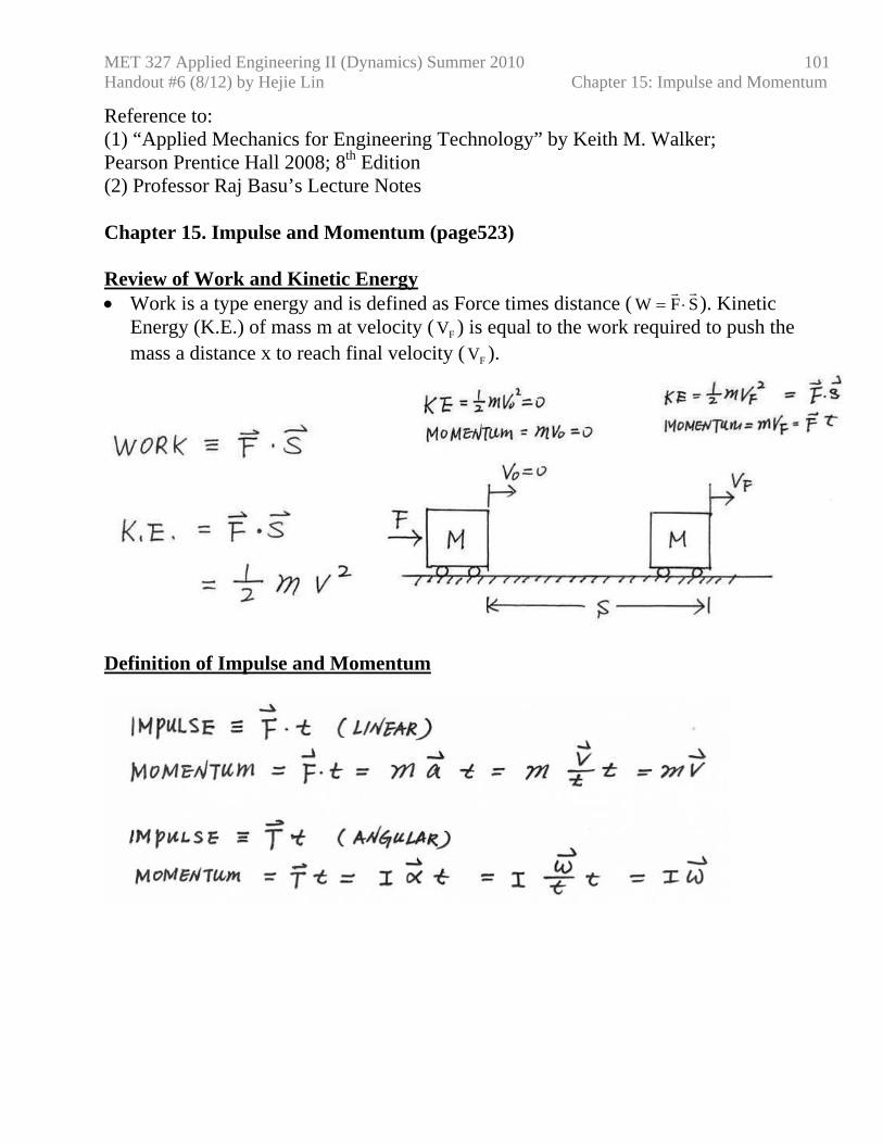
Reference to: (1) “Applied Mechanics for Engineering Technology” by Keith M. Walker; Pearson Prentice Hall 2008; 8th Edition (2) Professor Raj Basu’s Lecture Notes Chapter 15. Impulse and Momentum (page523) Review of Work and Kinetic Energy • Work is a type energy and is defined as Force times distance ( SFW
rr⋅= ). Kinetic
Energy (K.E.) of mass m at velocity ( FV ) is equal to the work required to push the mass a distance x to reach final velocity ( FV ).
Definition of Impulse and Momentum
MET 327 Applied Engineering II (Dynamics) Summer 2010 Handout #6 (8/12) by Hejie Lin Chapter 15: Impulse and Momentum
102
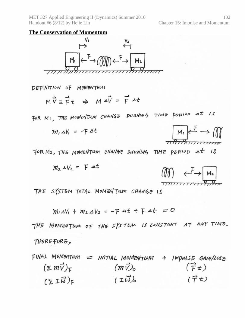
The Conservation of Momentum
MET 327 Applied Engineering II (Dynamics) Summer 2010 Handout #6 (8/12) by Hejie Lin Chapter 15: Impulse and Momentum
103
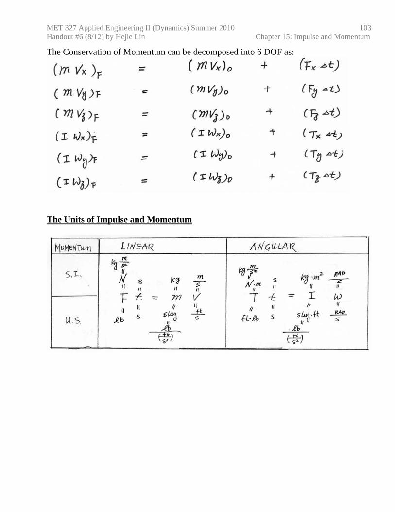
The Conservation of Momentum can be decomposed into 6 DOF as:
The Units of Impulse and Momentum
MET 327 Applied Engineering II (Dynamics) Summer 2010 Handout #6 (8/12) by Hejie Lin Chapter 15: Impulse and Momentum
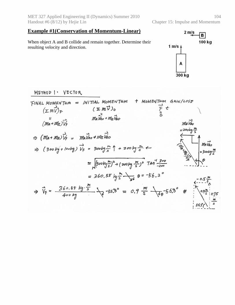
104
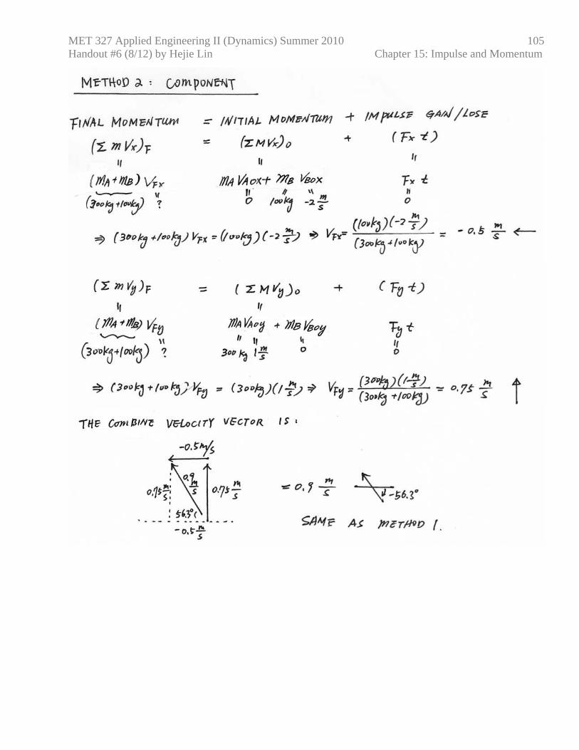
Example #1(Conservation of Momentum-Linear) When object A and B collide and remain together. Determine their resulting velocity and direction.
MET 327 Applied Engineering II (Dynamics) Summer 2010 Handout #6 (8/12) by Hejie Lin Chapter 15: Impulse and Momentum
105
MET 327 Applied Engineering II (Dynamics) Summer 2010 Handout #6 (8/12) by Hejie Lin Chapter 15: Impulse and Momentum
106
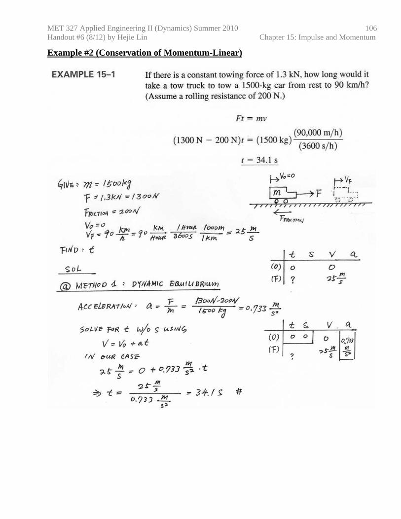
Example #2 (Conservation of Momentum-Linear)
MET 327 Applied Engineering II (Dynamics) Summer 2010 Handout #6 (8/12) by Hejie Lin Chapter 15: Impulse and Momentum
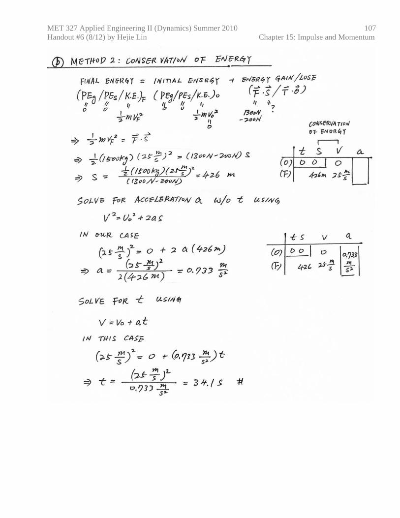
107
MET 327 Applied Engineering II (Dynamics) Summer 2010 Handout #6 (8/12) by Hejie Lin Chapter 15: Impulse and Momentum
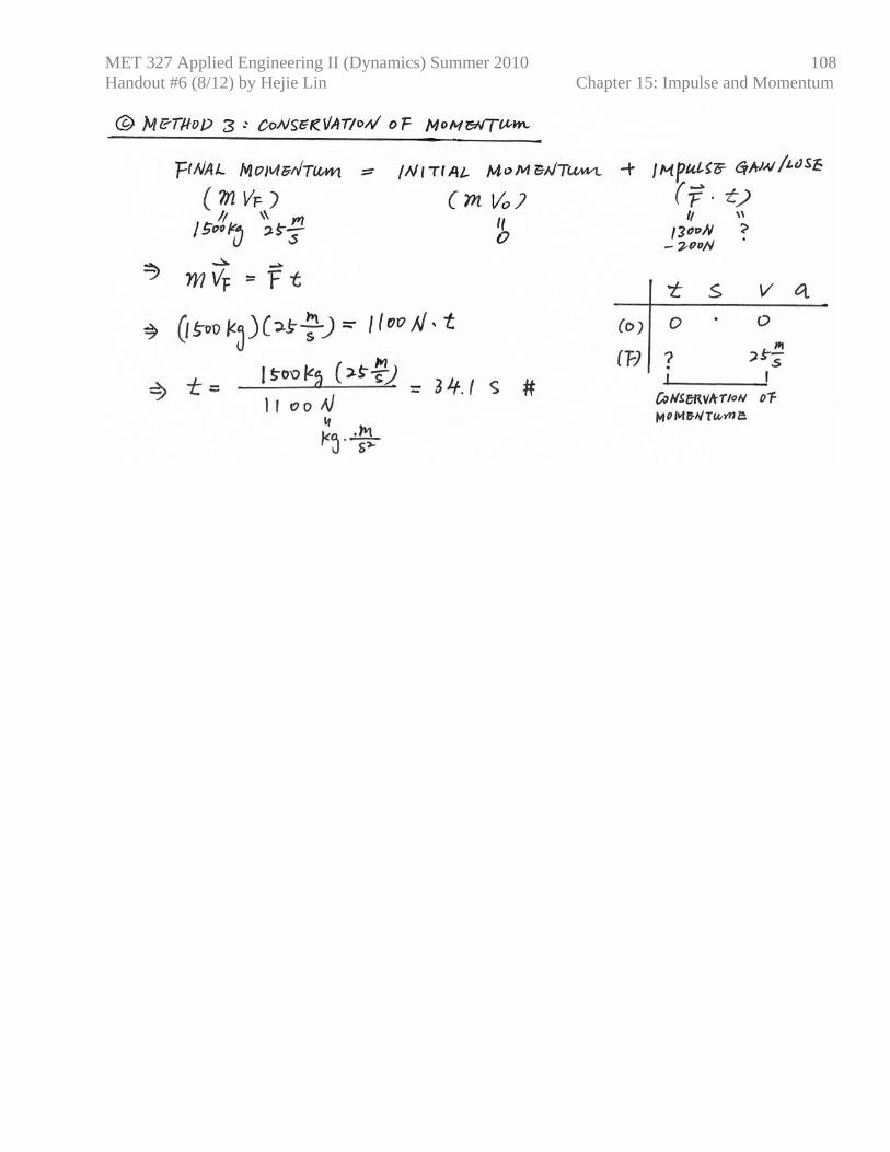
108
MET 327 Applied Engineering II (Dynamics) Summer 2010 Handout #6 (8/12) by Hejie Lin Chapter 15: Impulse and Momentum
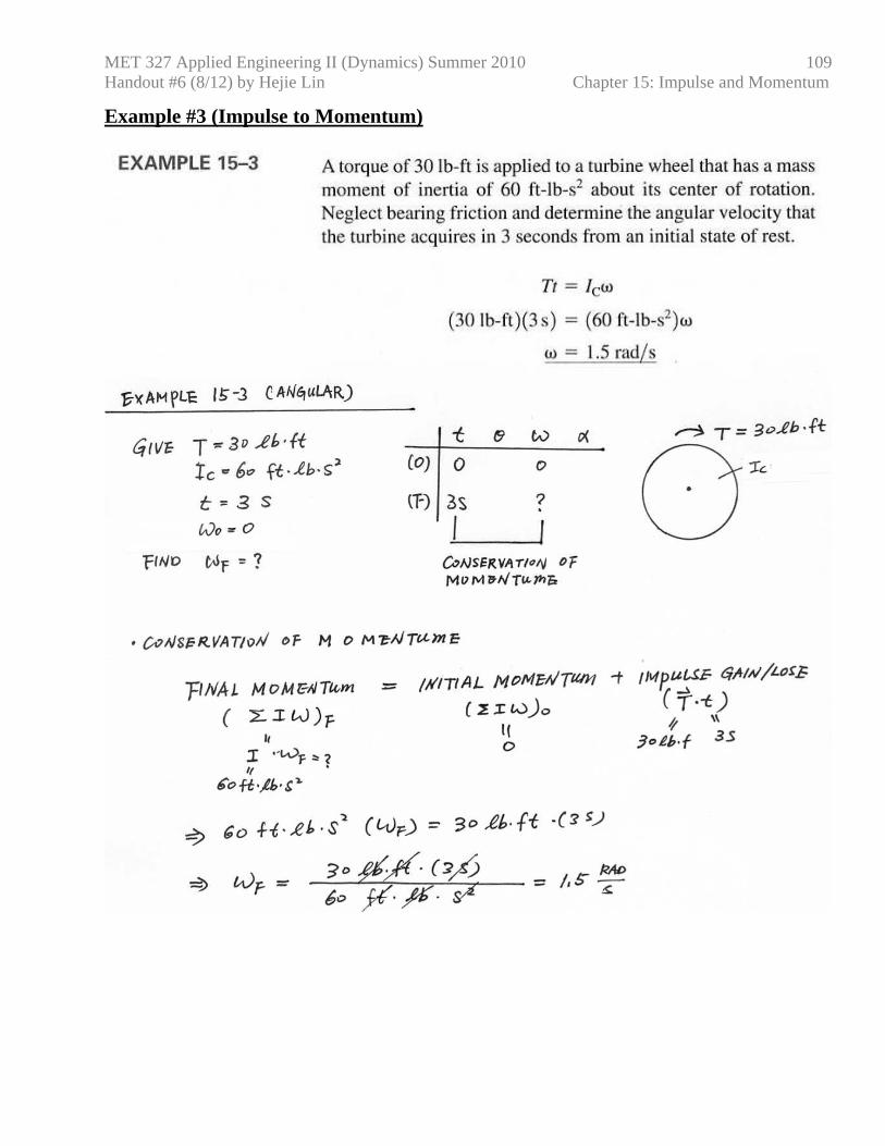
109
Example #3 (Impulse to Momentum)
MET 327 Applied Engineering II (Dynamics) Summer 2010 Handout #6 (8/12) by Hejie Lin Chapter 15: Impulse and Momentum
110
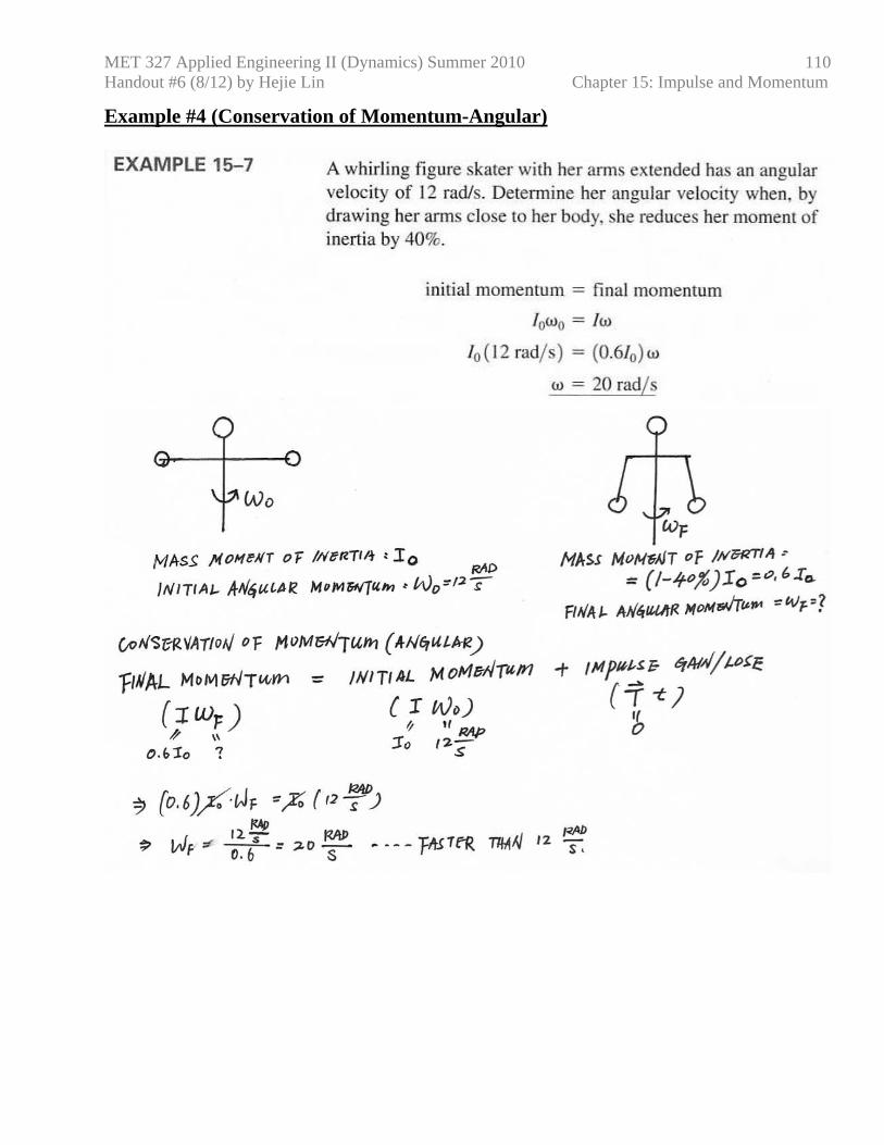
Example #4 (Conservation of Momentum-Angular)
MET 327 Applied Engineering II (Dynamics) Summer 2010 Handout #6 (8/12) by Hejie Lin Chapter 15: Impulse and Momentum
111
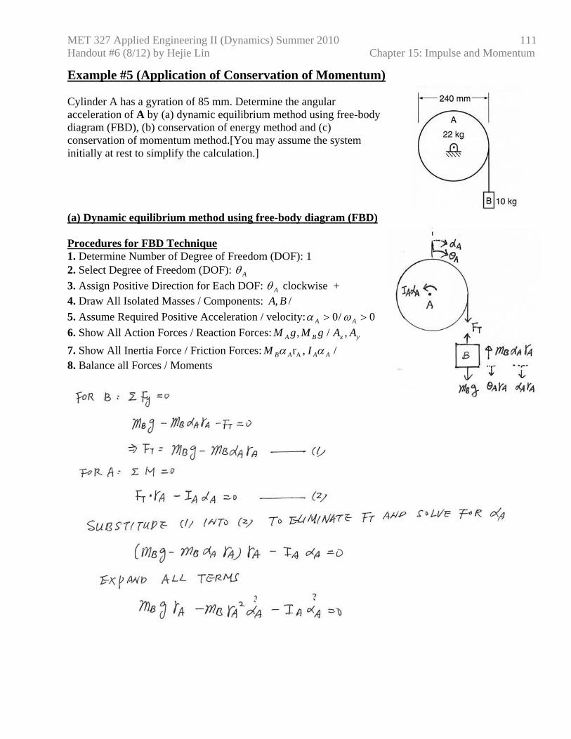
Example #5 (Application of Conservation of Momentum) Cylinder A has a gyration of 85 mm. Determine the angular acceleration of A by (a) dynamic equilibrium method using free-body diagram (FBD), (b) conservation of energy method and (c) conservation of momentum method.[You may assume the system initially at rest to simplify the calculation.] (a) Dynamic equilibrium method using free-body diagram (FBD) Procedures for FBD Technique 1. Determine Number of Degree of Freedom (DOF): 1 2. Select Degree of Freedom (DOF): Aθ 3. Assign Positive Direction for Each DOF: Aθ clockwise + 4. Draw All Isolated Masses / Components: /, BA 5. Assume Required Positive Acceleration / velocity: 0/ 0 >> AA ωα 6. Show All Action Forces / Reaction Forces: yxBA AAgMgM , / , 7. Show All Inertia Force / Friction Forces: / ,rA AAAB IM αα 8. Balance all Forces / Moments
MET 327 Applied Engineering II (Dynamics) Summer 2010 Handout #6 (8/12) by Hejie Lin Chapter 15: Impulse and Momentum
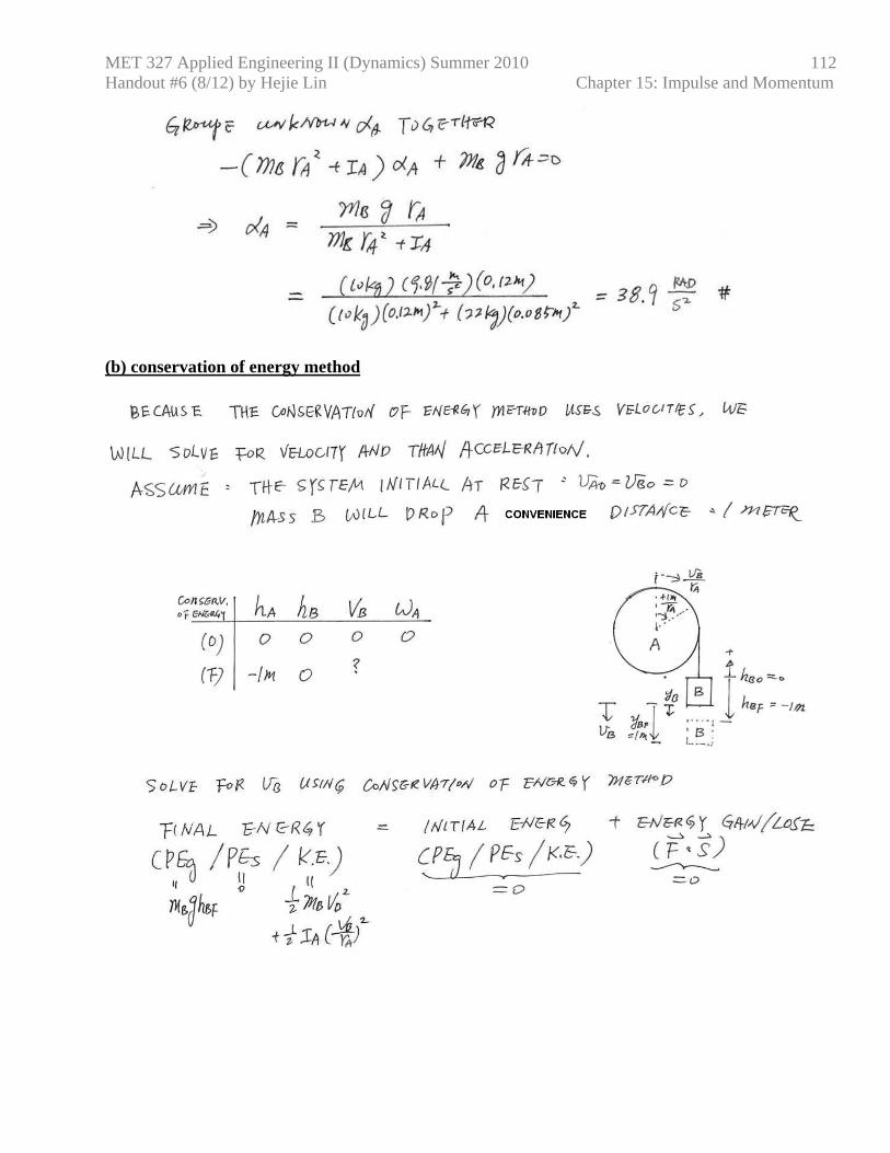
112
(b) conservation of energy method
MET 327 Applied Engineering II (Dynamics) Summer 2010 Handout #6 (8/12) by Hejie Lin Chapter 15: Impulse and Momentum
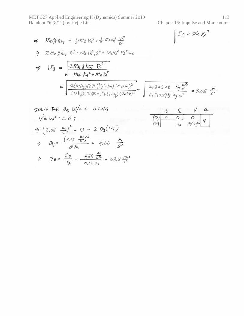
113
MET 327 Applied Engineering II (Dynamics) Summer 2010 Handout #6 (8/12) by Hejie Lin Chapter 15: Impulse and Momentum
114
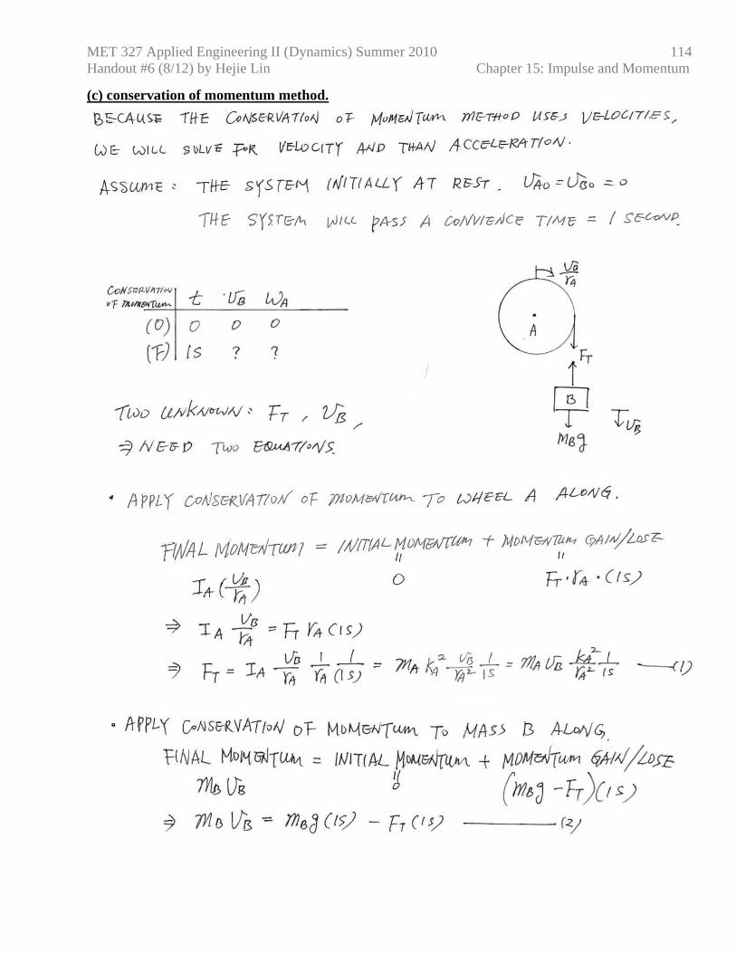
(c) conservation of momentum method.
MET 327 Applied Engineering II (Dynamics) Summer 2010 Handout #6 (8/12) by Hejie Lin Chapter 15: Impulse and Momentum
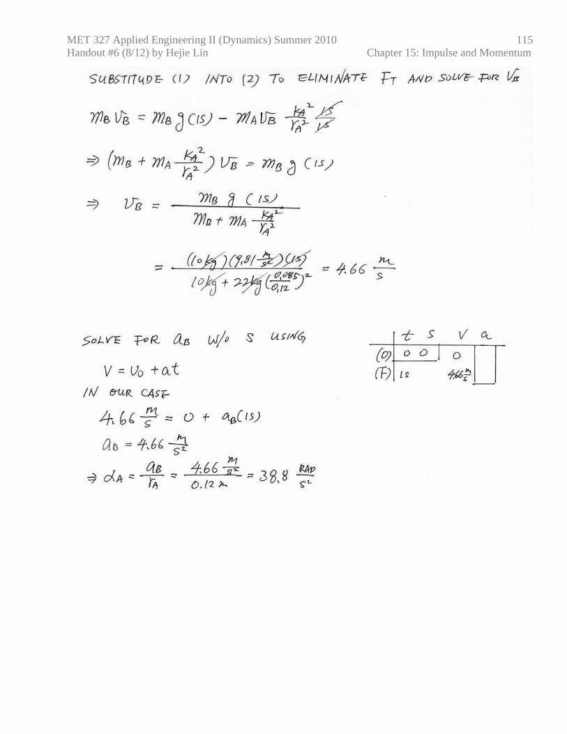
115
MET 327 Applied Engineering II (Dynamics) Summer 2010 Handout #6 (8/12) by Hejie Lin Chapter 15: Impulse and Momentum
116
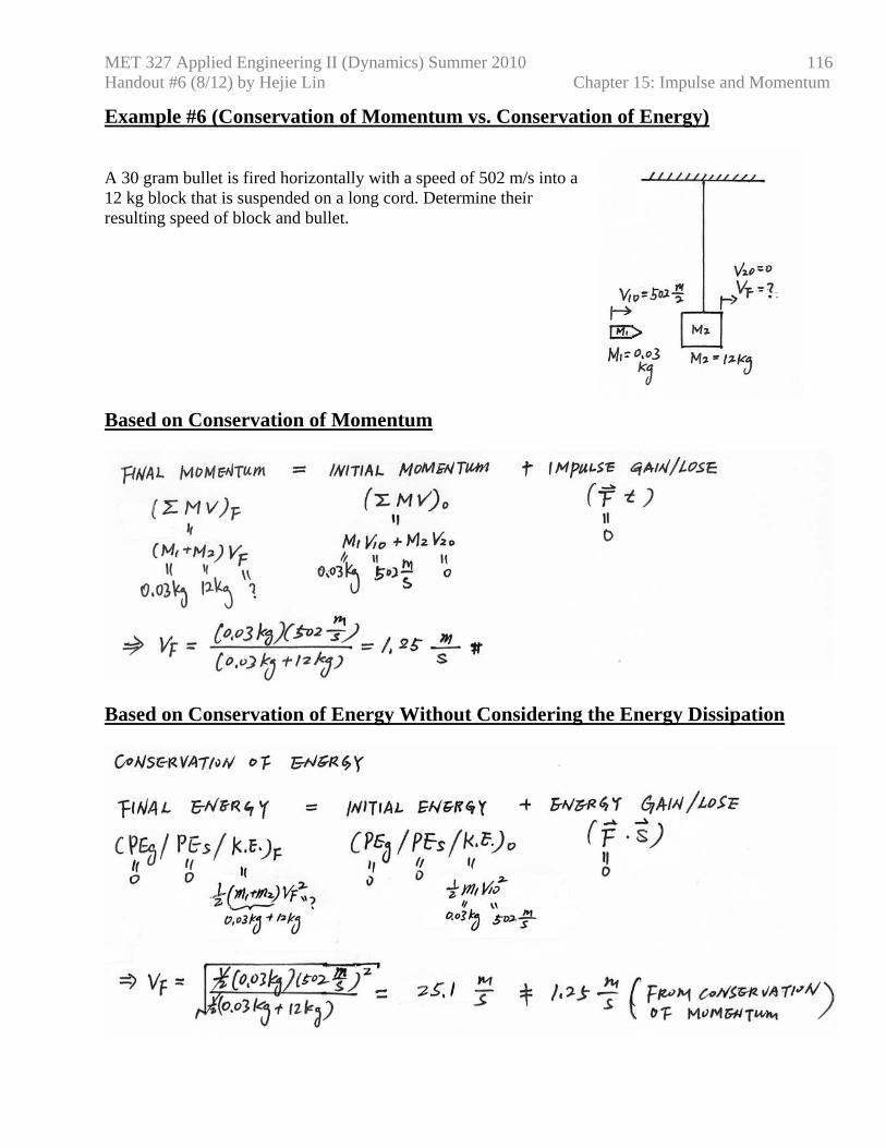
Example #6 (Conservation of Momentum vs. Conservation of Energy) A 30 gram bullet is fired horizontally with a speed of 502 m/s into a 12 kg block that is suspended on a long cord. Determine their resulting speed of block and bullet. Based on Conservation of Momentum
Based on Conservation of Energy Without Considering the Energy Dissipation
MET 327 Applied Engineering II (Dynamics) Summer 2010 Handout #6 (8/12) by Hejie Lin Chapter 15: Impulse and Momentum
117
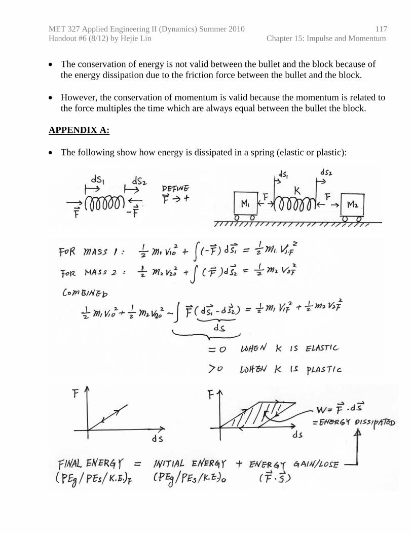
• The conservation of energy is not valid between the bullet and the block because of
the energy dissipation due to the friction force between the bullet and the block. • However, the conservation of momentum is valid because the momentum is related to
the force multiples the time which are always equal between the bullet the block. APPENDIX A: • The following show how energy is dissipated in a spring (elastic or plastic):
MET 327 Applied Engineering II (Dynamics) Summer 2010 Handout #6 (8/12) by Hejie Lin Chapter 15: Impulse and Momentum
118
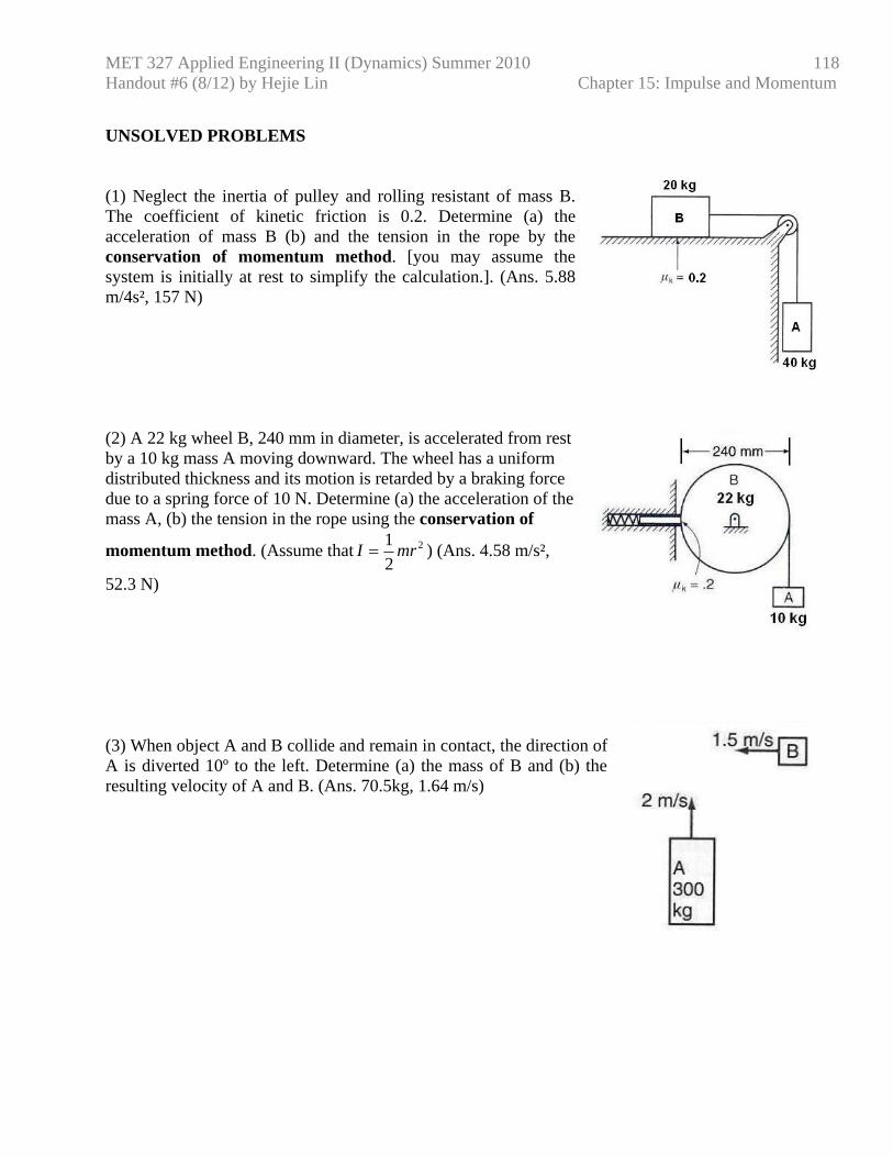
UNSOLVED PROBLEMS (1) Neglect the inertia of pulley and rolling resistant of mass B. The coefficient of kinetic friction is 0.2. Determine (a) the acceleration of mass B (b) and the tension in the rope by the conservation of momentum method. [you may assume the system is initially at rest to simplify the calculation.]. (Ans. 5.88 m/4s², 157 N) (2) A 22 kg wheel B, 240 mm in diameter, is accelerated from rest by a 10 kg mass A moving downward. The wheel has a uniform distributed thickness and its motion is retarded by a braking force due to a spring force of 10 N. Determine (a) the acceleration of the mass A, (b) the tension in the rope using the conservation of
momentum method. (Assume that 2
21 mrI = ) (Ans. 4.58 m/s²,
52.3 N) (3) When object A and B collide and remain in contact, the direction of A is diverted 10º to the left. Determine (a) the mass of B and (b) the resulting velocity of A and B. (Ans. 70.5kg, 1.64 m/s)