Embed Size (px)
Citation preview

METODOS DIRECTOS PARAGRANDES SISTEMAS DE ECUACIONES LINEALES:
FACTORIZACIONES DE CROUT Y CHOLESKYF. Navarrina, I. Colominas, M. Casteleiro, H. Gomez, J. Parıs
GMNI — GRUPO DE METODOS NUMERICOS EN INGENIERIA
Departamento de Metodos Matematicos y de RepresentacionEscuela Tecnica Superior de Ingenieros de Caminos, Canales y Puertos
Universidad de A Coruna, Espana
e-mail: [email protected] web: http://caminos.udc.es/gmni
UNIVERSIDAD DE A CORUNA — GRUPO DE METODOS NUMERICOS EN INGENIERIA

INDICE
I FACTORIZACION DE CROUT A˜ = L˜ D˜ U˜• Fundamentos teoricos. Condiciones de existencia• Algoritmos de factorizacion y de solucion de sistemas• Programacion. Almacenamiento de los resultados sobre los datos• Adaptacion para almacenamientos en banda y perfil
I FACTORIZACION DE CHOLESKY A˜ = L˜ D˜ L˜T
• Fundamentos teoricos. Condiciones de existencia• Algoritmos de factorizacion y de solucion de sistemas• Programacion. Almacenamiento de los resultados sobre los datos• Adaptacion para almacenamientos en banda y perfil
ICONDICIONES DE VINCULACION [coacciones]
I IMPLEMENTACION• Metodo de Cholesky para matrices en perfil (“Column Profile” o “Sky-Line”)
UNIVERSIDAD DE A CORUNA — GRUPO DE METODOS NUMERICOS EN INGENIERIA

FACTORIZACION DE CROUT: Fundamentos Teoricos (I)
FACTORIZACION DE CROUT [A˜ = L˜ D˜ U˜ ]
Sea el problema
A˜ x = b con A˜ =
a11 a12 · · · a1n
a21 a22 · · · a2n... ... . . . ...an1 an2 · · · ann
, x =
x1
x2...xn
, b =
b1
b2...bn
.
La FACTORIZACION DE CROUT consiste en:
A˜ = L˜ D˜ U˜ =⇒ L˜z︷ ︸︸ ︷
D˜ U˜ x︸︷︷︸y
= b =⇒
L˜ z = b,
D˜ y = z,
U˜ x = y.
UNIVERSIDAD DE A CORUNA — GRUPO DE METODOS NUMERICOS EN INGENIERIA

FACTORIZACION DE CROUT: Fundamentos Teoricos (IIa)
FUNCIONAMIENTO DEL METODO
Supongamos que ya hemos factorizado
A˜k = L˜k D˜ k U˜k, con A˜k =
[a11 · · · a1k... . . . ...ak1 · · · akk
],
siendo
L˜k =
[l11 0... . . .
lk1 · · · lkk
], D˜ k =
[d11 0
. . .0 dkk
], U˜k =
[u11 · · · u1k. . . ...0 ukk
].
UNIVERSIDAD DE A CORUNA — GRUPO DE METODOS NUMERICOS EN INGENIERIA

FACTORIZACION DE CROUT: Fundamentos Teoricos (IIb)
Pretendemos factorizar (a partir de lo anterior)
A˜k+1 = L˜k+1 D˜ k+1 U˜k+1, con A˜k+1 =
A˜k ck+1
fTk+1
ak+1,k+1
,
de forma que
Lek+1 =
266666664Lek 0
lTk+1lk+1,k+1
377777775, De k+1 =
266666664De k 0
0T dk+1,k+1
377777775, Uek+1 =
26666666664
Uek uk+1
0T uk+1,k+1
37777777775.
donde
ck+1 =
8<:a1,k+1
...ak,k+1
9=; , uk+1 =
8<:u1,k+1
...uk,k+1
9=; ,
fTk+1 = [ ak+1,1 · · · ak+1,k ] , l
Tk+1 = [ lk+1,1 · · · lk+1,k ] .
UNIVERSIDAD DE A CORUNA — GRUPO DE METODOS NUMERICOS EN INGENIERIA

FACTORIZACION DE CROUT: Fundamentos Teoricos (IIc)
Multiplicamos por cajas . . .
De k+1 Uek+1 =
266666666666664
De k Uek +
0ez|0 0
TDe k uk+1 +
0z | 0 uk+1,k+1
0T
Uek
| z 0
T
+ dk+1,k+1 0T
| z 0
T
0T
uk+1
| z 0
+ dk+1,k+1 uk+1,k+1
377777777777775.
Lek+1
`De k+1 Uek+1
´=
266666666666664
Lek De k Uek +
0ez|0 0
TLek De k uk+1 +
0z | 0 dk+1,k+1 uk+1,k+1
lTk+1De k Uek + lk+1,k+1 0T
| z 0
T
lTk+1De k uk+1 + lk+1,k+1 dk+1,k+1 uk+1,k+1
377777777777775.
UNIVERSIDAD DE A CORUNA — GRUPO DE METODOS NUMERICOS EN INGENIERIA

FACTORIZACION DE CROUT: Fundamentos Teoricos (IId)
Igualamos . . .266666664Aek ck+1
fTk+1
ak+1,k+1
377777775=
266666664Lek De k Uek Lek De k uk+1
lTk+1De k Uek lTk+1De k uk+1 + lk+1,k+1 dk+1,k+1 uk+1,k+1
377777775,
lo que por cajas equivale a
A˜k = L˜k D˜ k U˜k, [⇐ HIPOTESIS]
ck+1 = L˜k D˜ k uk+1 ,
fTk+1 = lTk+1 D˜ k U˜k,
ak+1,k+1 = lTk+1 D˜ k uk+1 + lk+1,k+1 dk+1,k+1 uk+1,k+1 .
UNIVERSIDAD DE A CORUNA — GRUPO DE METODOS NUMERICOS EN INGENIERIA

FACTORIZACION DE CROUT: Fundamentos Teoricos (IIe)
Por tanto . . .
1. El vector uk+1 es la solucıon del sistema:
[L˜k D˜ k] uk+1 = ck+1 .
2. El vector lk+1 es la solucıon del sistema:[U˜T
k D˜ k
]lk+1 = fk+1 .
3. Los coeficientes lk+1,k+1, dk+1,k+1 y uk+1,k+1 verifican:
lk+1,k+1 dk+1,k+1 uk+1,k+1 = ak+1,k+1 − lTk+1D˜ k uk+1. (*)
(*) Donde lk+1 y uk+1 se habran calculado previamente.Hay infinitas descomposiciones posibles. Por convenio, se eligen (arbitrariamente) los valores:
lk+1,k+1 = 1, uk+1,k+1 = 1 =⇒ dk+1,k+1 = ak+1,k+1 − lTk+1De k uk+1.
UNIVERSIDAD DE A CORUNA — GRUPO DE METODOS NUMERICOS EN INGENIERIA

FACTORIZACION DE CROUT: Fundamentos Teoricos (IIf)
4. Para k = 1:
A˜1 = L˜1 D˜ 1 U˜1 =⇒ l11 d11 u11 = a11 . (*)
5. Para k = n:
A˜n = A˜ =⇒ A˜ = L˜ D˜ U˜ con
L˜ = L˜n,
D˜ = D˜ n,
U˜ = U˜n.
(*) Hay infinitas descomposiciones posibles. Por convenio, se eligen (arbitrariamente) los valores:
l11 = 1, u11 = 1 =⇒ d11 = a11 .
UNIVERSIDAD DE A CORUNA — GRUPO DE METODOS NUMERICOS EN INGENIERIA

FACTORIZACION DE CROUT: Fundamentos Teoricos (IIIa)
REALIZACION DE LOS CALCULOS
1. FACTORIZACION DE LA MATRIZ:
Asignar l11 = 1, u11 = 1,
d11 = a11 .
Para k = 1, . . . , n− 1
Resolver[L˜k D˜ k
]uk+1 = ck+1 ,
[U˜k
TD˜ k
]lk+1 = fk+1 .
Asignar lk+1,k+1 = 1, uk+1,k+1 = 1,
dk+1,k+1 = ak+1,k+1 − lTk+1D˜ k uk+1.
UNIVERSIDAD DE A CORUNA — GRUPO DE METODOS NUMERICOS EN INGENIERIA

FACTORIZACION DE CROUT: Fundamentos Teoricos (IIIb)
Notas:
1. Los sistemas [L˜k D˜ k] uk+1 = ck+1 se resuelven en dos fases:
L˜k
vk+1︷ ︸︸ ︷D˜ k uk+1 = ck+1 =⇒
L˜k vk+1 = ck+1,
D˜ k uk+1 = vk+1.
2. Los sistemas[U˜T
k D˜ k
]lk+1 = fk+1 se resuelven en dos fases:
U˜Tk
mk+1︷ ︸︸ ︷D˜ k lk+1 = fk+1 =⇒
U˜T
k mk+1 = fk+1,
D˜ k lk+1 = mk+1.
UNIVERSIDAD DE A CORUNA — GRUPO DE METODOS NUMERICOS EN INGENIERIA
FACTORIZACION DE CROUT: Fundamentos Teoricos (IIIc)
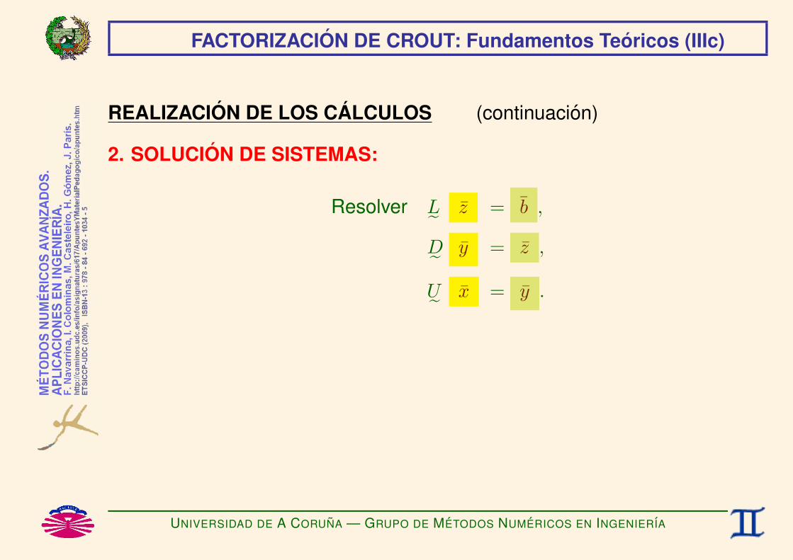
REALIZACION DE LOS CALCULOS (continuacion)
2. SOLUCION DE SISTEMAS:
Resolver L˜ z = b ,
D˜ y = z ,
U˜ x = y .
UNIVERSIDAD DE A CORUNA — GRUPO DE METODOS NUMERICOS EN INGENIERIA

FACTORIZACION DE CROUT: Fundamentos Teoricos (IVa)
CONDICIONES DE EXISTENCIAPor construccion (unos en la diagonal principal), se cumple
det(Lek) = det(Uek) = 1 para k = 1, . . . , n.
Por tanto, basta con que se cumplan las condiciones(det(De k) 6= 0, k = 1, . . . , n− 1 para que pueda realizarse la factorizacion,
det(De k) 6= 0, k = n para que pueda realizarse la solucion de sistemas.
Por otro lado,
Aek = Lek De k Uek =⇒ det(Aek) = det(Lek) det(De k) det(Uek) = det(De k) ∀k.
Luego, las condiciones de existencia pueden expresarse en la forma
(det(Aek) 6= 0, k = 1, . . . , n− 1 para que pueda realizarse la factorizacion,
det(Aek) 6= 0, k = n para que pueda realizarse la solucion de sistemas.
UNIVERSIDAD DE A CORUNA — GRUPO DE METODOS NUMERICOS EN INGENIERIA

FACTORIZACION DE CROUT: Fundamentos Teoricos (IVb)
En general, podemos afirmar que:
♥ Si la matriz es REGULARhdet(Ae) 6= 0
i. . .
♠ puede pasar que la factorizacion exista; (*)
♠ puede pasar que la factorizacion NO exista; (**)
♠ es practicamente imposible comprobar a priori la condicion de existencia anterior;
♣ es sencillo (y RECOMENDABLE en todo caso) comprobar sobre la marcha que
d11 6= 0, dk+1,k+1 6= 0 para k = 1, . . . , n.
♠ Aunque la matriz sea SINGULARhdet(Ae) = 0
i. . .
♠ puede pasar que la factorizacion exista; (*)
♠ pero no se podra utilizar para resolver el sistema. (***)
(*) Esto sucedera cuando det(Aek) 6= 0, k = 1, . . . , n− 1.
(**) Esto sucedera cuando no se cumpla la condicion anterior. Por ejemplo, cuando a11 = 0.Al igual que en el Metodo de Gauss, estos casos requieren PIVOTAMIENTO (intercambio de filas y/o columnas).El problema es que el pivotamiento casa mal con los almacenamientos en banda y en perfil.
(***) Porque el sistema no tiene solucion y el algoritmo fallara al resolver De y = z .
UNIVERSIDAD DE A CORUNA — GRUPO DE METODOS NUMERICOS EN INGENIERIA
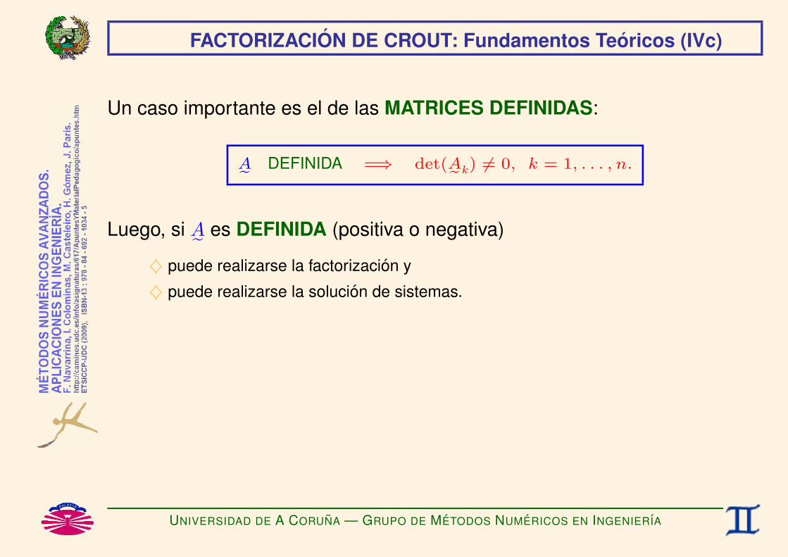
FACTORIZACION DE CROUT: Fundamentos Teoricos (IVc)
Un caso importante es el de las MATRICES DEFINIDAS:
Ae DEFINIDA =⇒ det(Aek) 6= 0, k = 1, . . . , n.
Luego, si A˜ es DEFINIDA (positiva o negativa)
♦ puede realizarse la factorizacion y
♦ puede realizarse la solucion de sistemas.
UNIVERSIDAD DE A CORUNA — GRUPO DE METODOS NUMERICOS EN INGENIERIA

FACTORIZACION DE CROUT: Algoritmos (I)
1. FACTORIZACION DE LA MATRIZ:
l11 = 1, u11 = 1
d11 = a11
DO k=1,n-1
ui,k+1 = ai,k+1 −i−1Xj=1
lij uj,k+1 ; i = 1, . . . , k
ui,k+1 = ui,k+1 / dii ; i = 1, . . . , k
lk+1,i = ak+1,i −i−1Xj=1
uji lk+1,j ; i = 1, . . . , k
lk+1,i = lk+1,i / dii ; i = 1, . . . , k
lk+1,k+1 = 1, uk+1,k+1 = 1
dk+1,k+1 = ak+1,k+1 −kX
j=1
lk+1,j djj uj,k+1
ENDDO
UNIVERSIDAD DE A CORUNA — GRUPO DE METODOS NUMERICOS EN INGENIERIA

FACTORIZACION DE CROUT: Algoritmos (II)
2. SOLUCION DE SISTEMAS: (*)
zi = bi −i−1Xj=1
lij zj ; i = 1, . . . , n
yi = zi / dii ; i = 1, . . . , n
xi = yi −nX
j=i+1
uij xj ; i = n, . . . , 1,−1
(*) Este planteamiento es adecuado para matrices en banda pero inadecuado para matrices en perfildebido a que el bucle interno de la ultima expresion (sumatorio) barre la matriz Ue por filas.
UNIVERSIDAD DE A CORUNA — GRUPO DE METODOS NUMERICOS EN INGENIERIA

FACTORIZACION DE CROUT: Algoritmos (III)
2. SOLUCION DE SISTEMAS: [Planteamiento Alternativo] (*)
zi = bi −i−1Xj=1
lij zj ; i = 1, . . . , n
yi = zi / dii ; i = 1, . . . , n
xi = yi ; i = 1, . . . , n
xj = xj − uji xi ; j = 1, . . . , i− 1 ; i = n, . . . , 2,−1
(*) Este planteamiento es adecuado para matrices en banda y tambien para matrices en perfil.Observese que el bucle interno de la ultima expresion barre ahora la matriz Ue por columnas.
UNIVERSIDAD DE A CORUNA — GRUPO DE METODOS NUMERICOS EN INGENIERIA

FACTORIZACION DE CROUT: Programacion (–)
Es facil comprobar que
• podemos almacenar L˜, D˜ y U˜ sobre A˜ ;
• podemos almacenar z, y y x sobre b;
Ası. . .a11 a12 a13 · · · a1n
a21 a22 a23 · · · a2n
a31 a32 a33 · · · a3n... ... ... . . . ...an1 an2 an3 · · · ann
se transformara en−→
d11 u12 u13 · · · u1n
l21 d22 u23 · · · u2n
l31 l32 d33 · · · u3n... ... ... . . . ...ln1 ln2 ln3 · · · dnn
.
b1
b2
b3...bn
se transformara en−→
z1
z2
z3...zn
se transformara en−→
y1
y2
y3...yn
se transformara en−→
x1
x2
x3...xn
.
UNIVERSIDAD DE A CORUNA — GRUPO DE METODOS NUMERICOS EN INGENIERIA
FACTORIZACION DE CROUT: Programacion (I)
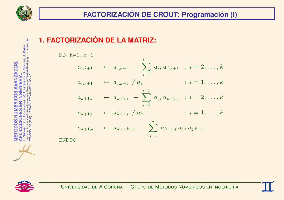
1. FACTORIZACION DE LA MATRIZ:
DO k=1,n-1
ai,k+1 ← ai,k+1 −i−1Xj=1
aij aj,k+1 ; i = 2, . . . , k
ai,k+1 ← ai,k+1 / aii ; i = 1, . . . , k
ak+1,i ← ak+1,i −i−1Xj=1
aji ak+1,j ; i = 2, . . . , k
ak+1,i ← ak+1,i / aii ; i = 1, . . . , k
ak+1,k+1 ← ak+1,k+1 −kX
j=1
ak+1,j ajj aj,k+1
ENDDO
UNIVERSIDAD DE A CORUNA — GRUPO DE METODOS NUMERICOS EN INGENIERIA

FACTORIZACION DE CROUT: Programacion (II)
2. SOLUCION DE SISTEMAS: (*)
bi ← bi −i−1Xj=1
aij bj ; i = 2, . . . , n
bi ← bi / aii ; i = 1, . . . , n
bi ← bi −nX
j=i+1
aij bj ; i = n−1, . . . , 1,−1
(*) Este planteamiento es adecuado para matrices en banda pero inadecuado para matrices en perfildebido a que el bucle interno de la ultima expresion (sumatorio) barre la parte superior de la matriz Ae por filas.
UNIVERSIDAD DE A CORUNA — GRUPO DE METODOS NUMERICOS EN INGENIERIA
FACTORIZACION DE CROUT: Programacion (III)
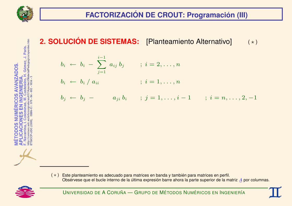
2. SOLUCION DE SISTEMAS: [Planteamiento Alternativo] (*)
bi ← bi −i−1Xj=1
aij bj ; i = 2, . . . , n
bi ← bi / aii ; i = 1, . . . , n
bj ← bj − aji bi ; j = 1, . . . , i− 1 ; i = n, . . . , 2,−1
(*) Este planteamiento es adecuado para matrices en banda y tambien para matrices en perfil.Observese que el bucle interno de la ultima expresion barre ahora la parte superior de la matriz Ae por columnas.
UNIVERSIDAD DE A CORUNA — GRUPO DE METODOS NUMERICOS EN INGENIERIA

FACTORIZACION DE CROUT: Adaptacion a Banda y Perfil (Ia)
Sea la matriz A˜ tal que
A˜ =
00
ai−u(i),i
...
...ai−1,i
0 0 ai,i−`(i) · · · · · · ai,i−1 aii −→ fila i
↓columna i
donde (
`(i) ≡ semiancho de banda inferior de la fila i,
u(i) ≡ semiancho de banda superior de la columna i.
UNIVERSIDAD DE A CORUNA — GRUPO DE METODOS NUMERICOS EN INGENIERIA

FACTORIZACION DE CROUT: Adaptacion a Banda y Perfil (Ib)
Examinamos en detalle el calculo
de la fila k + 1 de L˜, y
de la columna k + 1 de U˜ .
ui,k+1 = ai,k+1 −i−1Xj=1
lij uj,k+1 ; i = 1, . . . , k
ui,k+1 = ui,k+1 / dii ; i = 1, . . . , k −→ IRRELEVANTE
lk+1,i = ak+1,i −i−1Xj=1
uji lk+1,j ; i = 1, . . . , k
lk+1,i = lk+1,i / dii ; i = 1, . . . , k −→ IRRELEVANTE
UNIVERSIDAD DE A CORUNA — GRUPO DE METODOS NUMERICOS EN INGENIERIA

FACTORIZACION DE CROUT: Adaptacion a Banda y Perfil (Ic)
Observamos que (a falta de dividir por los elementos dii) . . .8>>>>>>>>>>>>>>>>>>>><>>>>>>>>>>>>>>>>>>>>:
i = 1 −→ ai,k+1 = 0 ⇒ ui,k+1 = ai,k+1 −i−1Xj=1
lij uj,k+1 = 0 ,
i = 2 −→ ai,k+1 = 0 ⇒ ui,k+1 = ai,k+1 −i−1Xj=1
lij uj,k+1 = 0 ,
...
i = (k + 1)− u(k + 1)− 1 −→ ai,k+1 = 0 ⇒ ui,k+1 = ai,k+1 −i−1Xj=1
lij uj,k+1 = 0 ,
i = (k + 1)− u(k + 1) −→ ai,k+1 6= 0 ⇒ ui,k+1 = ai,k+1 −i−1Xj=1
lij uj,k+1 = ai,k+1 6= 0 .
8>>>>>>>>>>>>>>>>>>>><>>>>>>>>>>>>>>>>>>>>:
i = 1 −→ ak+1,i = 0 ⇒ lk+1,i = ak+1,i −i−1Xj=1
uji lk+1,j = 0 ,
i = 2 −→ ak+1,i = 0 ⇒ lk+1,i = ak+1,i −i−1Xj=1
uji lk+1,j = 0 ,
...
i = (k + 1)− `(k + 1)− 1 −→ ak+1,i = 0 ⇒ lk+1,i = ak+1,i −i−1Xj=1
uji lk+1,j = 0 ,
i = (k + 1)− `(k + 1) −→ ak+1,i 6= 0 ⇒ lk+1,i = ak+1,i −i−1Xj=1
uji lk+1,j = ak+1,i 6= 0 .
UNIVERSIDAD DE A CORUNA — GRUPO DE METODOS NUMERICOS EN INGENIERIA

FACTORIZACION DE CROUT: Adaptacion a Banda y Perfil (II)
Por tanto, se conservan los semianchos de banda inferior y superior:
Y tambien los perfiles inferior (por filas) y superior (por columnas):
UNIVERSIDAD DE A CORUNA — GRUPO DE METODOS NUMERICOS EN INGENIERIA

FACTORIZACION DE CHOLESKY: Fundamentos Teoricos (I)
FACTORIZACION DE CHOLESKY [A˜ = L˜ D˜ L˜T , A˜ simetrica]
Sea el problema
A˜ x = b con A˜ =
a11 a12 · · · a1n
a22 · · · a2n. . . ...Sim. ann
, x =
x1
x2...xn
, b =
b1
b2...bn
.
La FACTORIZACION DE CHOLESKY consiste en:
A˜ = L˜ D˜ L˜T =⇒ L˜z︷ ︸︸ ︷
D˜ L˜T x︸ ︷︷ ︸y
= b =⇒
L˜ z = b,
D˜ y = z,
L˜T x = y.
UNIVERSIDAD DE A CORUNA — GRUPO DE METODOS NUMERICOS EN INGENIERIA

FACTORIZACION DE CHOLESKY: Fundamentos Teoricos (IIa)
FUNCIONAMIENTO DEL METODO
Observamos que es un caso particular de la Factorizacion de CROUT paramatrices simetricas en el que
U˜ = L˜T .
Debido a la simetrıa se cumplira
ck+1 = fk+1 ,
U˜k = L˜Tk ,
uk+1 = lk+1 ,
uk+1,k+1 = lk+1,k+1 .
UNIVERSIDAD DE A CORUNA — GRUPO DE METODOS NUMERICOS EN INGENIERIA

FACTORIZACION DE CHOLESKY: Fundamentos Teoricos (IIb)
Por tanto . . .
1-2. El vector lk+1 es la solucıon del sistema:
[L˜k D˜ k] lk+1 = fk+1 .
3. Los coeficientes lk+1,k+1 y dk+1,k+1 verifican:
lk+1,k+1 dk+1,k+1 lk+1,k+1 = ak+1,k+1 − lTk+1D˜ k lk+1. (*)
(*) Donde lk+1 se habra calculado previamente.Hay infinitas descomposiciones posibles. Por convenio, se eligen (arbitrariamente) los valores:
lk+1,k+1 = 1 =⇒ dk+1,k+1 = ak+1,k+1 − lTk+1De k lk+1.
UNIVERSIDAD DE A CORUNA — GRUPO DE METODOS NUMERICOS EN INGENIERIA

FACTORIZACION DE CHOLESKY: Fundamentos Teoricos (IIc)
4. Para k = 1:
A˜1 = L˜1 D˜ 1 L˜T1 =⇒ l11 d11 l11 = a11 . (*)
5. Para k = n:
A˜n = A˜ =⇒ A˜ = L˜ D˜ L˜T con
L˜ = L˜n,
D˜ = D˜ n.
(*) Hay infinitas descomposiciones posibles. Por convenio, se eligen (arbitrariamente) los valores:
l11 = 1 =⇒ d11 = a11 .
UNIVERSIDAD DE A CORUNA — GRUPO DE METODOS NUMERICOS EN INGENIERIA
FACTORIZACION DE CHOLESKY: Fundamentos Teoricos (IIIa)
REALIZACION DE LOS CALCULOS
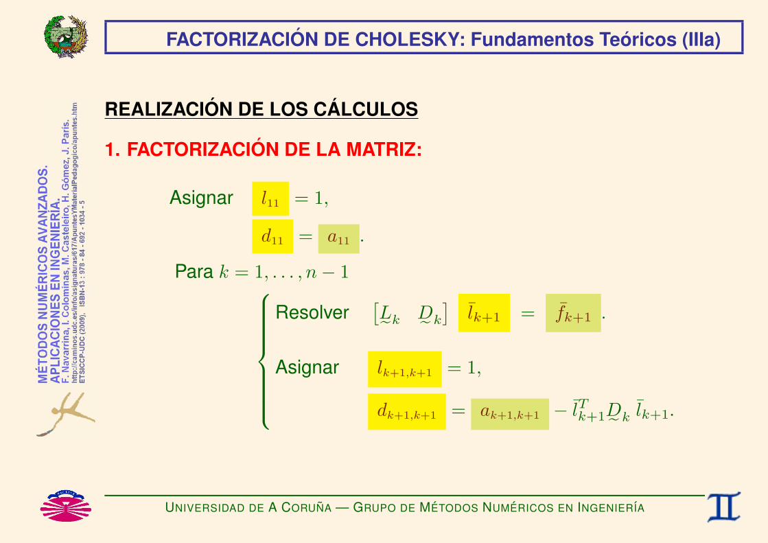
1. FACTORIZACION DE LA MATRIZ:
Asignar l11 = 1,
d11 = a11 .
Para k = 1, . . . , n− 1
Resolver[L˜k D˜ k
]lk+1 = fk+1 .
Asignar lk+1,k+1 = 1,
dk+1,k+1 = ak+1,k+1 − lTk+1D˜ k lk+1.
UNIVERSIDAD DE A CORUNA — GRUPO DE METODOS NUMERICOS EN INGENIERIA

FACTORIZACION DE CHOLESKY: Fundamentos Teoricos (IIIb)
Notas:
1. Los sistemas [L˜k D˜ k] lk+1 = fk+1 se resuelven en dos fases:
L˜k
mk+1︷ ︸︸ ︷D˜ k lk+1 = fk+1 =⇒
L˜k mk+1 = fk+1,
D˜ k lk+1 = mk+1.
UNIVERSIDAD DE A CORUNA — GRUPO DE METODOS NUMERICOS EN INGENIERIA

FACTORIZACION DE CHOLESKY: Fundamentos Teoricos (IIIc)
REALIZACION DE LOS CALCULOS (continuacion)
2. SOLUCION DE SISTEMAS:
Resolver L˜ z = b ,
D˜ y = z ,
L˜T x = y .
UNIVERSIDAD DE A CORUNA — GRUPO DE METODOS NUMERICOS EN INGENIERIA
FACTORIZACION DE CHOLESKY: Fundamentos Teoricos (IV)
CONDICIONES DE EXISTENCIA
Son las mismas que en el caso de la Factorizacion de CROUT.
UNIVERSIDAD DE A CORUNA — GRUPO DE METODOS NUMERICOS EN INGENIERIA

FACTORIZACION DE CHOLESKY: Algoritmos (I)
1. FACTORIZACION DE LA MATRIZ:
l11 = 1,
d11 = a11
DO k=1,n-1
lk+1,i = ak+1,i −i−1Xj=1
lij lk+1,j ; i = 1, . . . , k
lk+1,i = lk+1,i / dii ; i = 1, . . . , k
lk+1,k+1 = 1,
dk+1,k+1 = ak+1,k+1 −kX
j=1
lk+1,j djj lk+1,j
ENDDO
UNIVERSIDAD DE A CORUNA — GRUPO DE METODOS NUMERICOS EN INGENIERIA
FACTORIZACION DE CHOLESKY: Algoritmos (II)
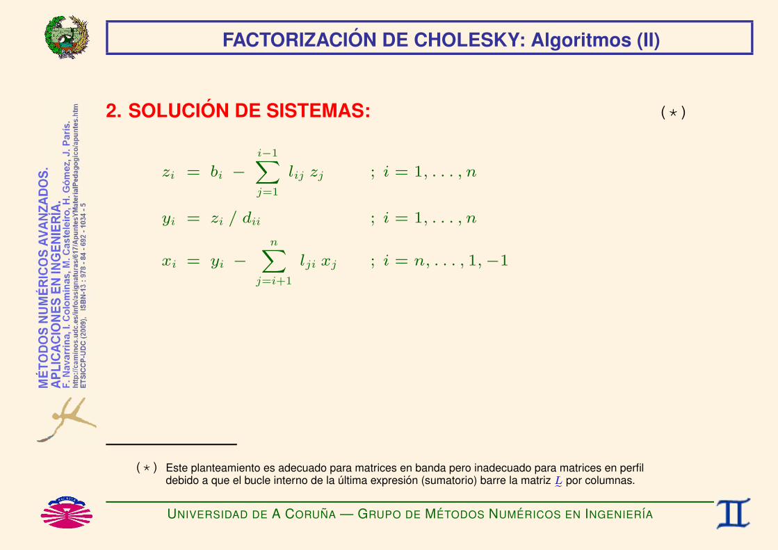
2. SOLUCION DE SISTEMAS: (*)
zi = bi −i−1Xj=1
lij zj ; i = 1, . . . , n
yi = zi / dii ; i = 1, . . . , n
xi = yi −nX
j=i+1
lji xj ; i = n, . . . , 1,−1
(*) Este planteamiento es adecuado para matrices en banda pero inadecuado para matrices en perfildebido a que el bucle interno de la ultima expresion (sumatorio) barre la matriz Le por columnas.
UNIVERSIDAD DE A CORUNA — GRUPO DE METODOS NUMERICOS EN INGENIERIA

FACTORIZACION DE CHOLESKY: Algoritmos (III)
2. SOLUCION DE SISTEMAS: [Planteamiento Alternativo] (*)
zi = bi −i−1Xj=1
lij zj ; i = 1, . . . , n
yi = zi / dii ; i = 1, . . . , n
xi = yi ; i = 1, . . . , n
xj = xj − lij xi ; j = 1, . . . , i− 1 ; i = n, . . . , 2,−1
(*) Este planteamiento es adecuado para matrices en banda y tambien para matrices en perfil.Observese que el bucle interno de la ultima expresion barre ahora la matriz Le por filas.
UNIVERSIDAD DE A CORUNA — GRUPO DE METODOS NUMERICOS EN INGENIERIA

FACTORIZACION DE CHOLESKY: Programacion (–)
Es facil comprobar que
• podemos almacenar L˜ Y D˜ sobre la parte inferior de A˜ ;
• podemos almacenar z, y y x sobre b;
Ası. . .a11
a21 a22
a31 a32 a33... ... ... . . .an1 an2 an3 · · · ann
se transformara en−→
d11
l21 d22
l31 l32 d33... ... ... . . .ln1 ln2 ln3 · · · dnn
.
b1
b2
b3...bn
se transformara en−→
z1
z2
z3...zn
se transformara en−→
y1
y2
y3...yn
se transformara en−→
x1
x2
x3...xn
.
UNIVERSIDAD DE A CORUNA — GRUPO DE METODOS NUMERICOS EN INGENIERIA

FACTORIZACION DE CHOLESKY: Programacion (I)
1. FACTORIZACION DE LA MATRIZ:
DO k=1,n-1
ak+1,i ← ak+1,i −i−1Xj=1
aij ak+1,j ; i = 2, . . . , k
ak+1,i ← ak+1,i / aii ; i = 1, . . . , k
ak+1,k+1 ← ak+1,k+1 −kX
j=1
ak+1,j ajj ak+1,j
ENDDO
UNIVERSIDAD DE A CORUNA — GRUPO DE METODOS NUMERICOS EN INGENIERIA
FACTORIZACION DE CHOLESKY: Programacion (II)
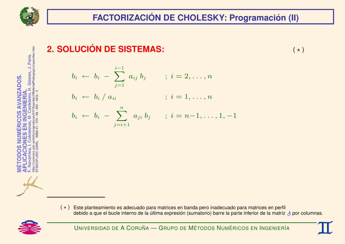
2. SOLUCION DE SISTEMAS: (*)
bi ← bi −i−1Xj=1
aij bj ; i = 2, . . . , n
bi ← bi / aii ; i = 1, . . . , n
bi ← bi −nX
j=i+1
aji bj ; i = n−1, . . . , 1,−1
(*) Este planteamiento es adecuado para matrices en banda pero inadecuado para matrices en perfildebido a que el bucle interno de la ultima expresion (sumatorio) barre la parte inferior de la matriz Ae por columnas.
UNIVERSIDAD DE A CORUNA — GRUPO DE METODOS NUMERICOS EN INGENIERIA

FACTORIZACION DE CHOLESKY: Programacion (III)
2. SOLUCION DE SISTEMAS: [Planteamiento Alternativo] (*)
bi ← bi −i−1Xj=1
aij bj ; i = 2, . . . , n
bi ← bi / aii ; i = 1, . . . , n
bj ← bj − aij bi ; j = 1, . . . , i− 1 ; i = n, . . . , 2,−1
(*) Este planteamiento es adecuado para matrices en banda y tambien para matrices en perfil.Observese que el bucle interno de la ultima expresion barre ahora la parte inferior de la matriz Ae por filas.
UNIVERSIDAD DE A CORUNA — GRUPO DE METODOS NUMERICOS EN INGENIERIA

FACTORIZACION DE CHOLESKY: Adaptacion a Banda y Perfil (Ia)
Sea la matriz A˜ tal que
A˜ =
SIM.
0 0 ai,i−`(i) · · · · · · ai,i−1 aii −→ fila i
↓columna i
donde (`(i) ≡ semiancho de banda inferior de la fila i,
≡ semiancho de banda superior de la columna i.
UNIVERSIDAD DE A CORUNA — GRUPO DE METODOS NUMERICOS EN INGENIERIA
FACTORIZACION DE CHOLESKY: Adaptacion a Banda y Perfil (Ib)
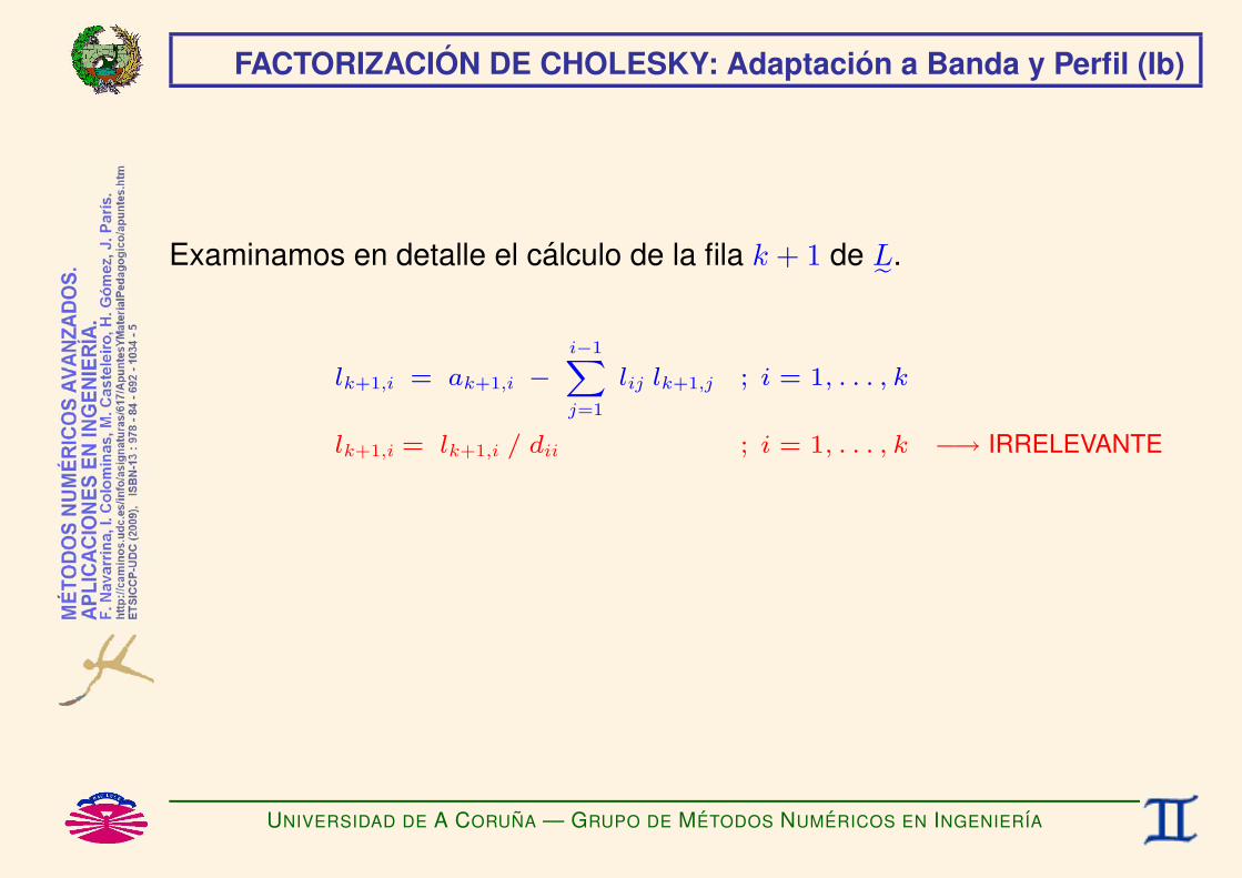
Examinamos en detalle el calculo de la fila k + 1 de L˜.
lk+1,i = ak+1,i −i−1Xj=1
lij lk+1,j ; i = 1, . . . , k
lk+1,i = lk+1,i / dii ; i = 1, . . . , k −→ IRRELEVANTE
UNIVERSIDAD DE A CORUNA — GRUPO DE METODOS NUMERICOS EN INGENIERIA

FACTORIZACION DE CHOLESKY: Adaptacion a Banda y Perfil (Ic)
Observamos que (a falta de dividir por los elementos dii) . . .
8>>>>>>>>>>>>>>>>>>>>>>>>>>>><>>>>>>>>>>>>>>>>>>>>>>>>>>>>:
i = 1 −→ ak+1,i = 0 ⇒ lk+1,i = ak+1,i −i−1Xj=1
lij lk+1,j = 0 ,
i = 2 −→ ak+1,i = 0 ⇒ lk+1,i = ak+1,i −i−1Xj=1
lij lk+1,j = 0 ,
...
i = (k + 1)− `(k + 1)− 1 −→ ak+1,i = 0 ⇒ lk+1,i = ak+1,i −i−1Xj=1
lij lk+1,j = 0 ,
i = (k + 1)− `(k + 1) −→ ak+1,i 6= 0 ⇒ lk+1,i = ak+1,i −i−1Xj=1
lij lk+1,j = ak+1,i 6= 0 .
UNIVERSIDAD DE A CORUNA — GRUPO DE METODOS NUMERICOS EN INGENIERIA

FACTORIZACION DE CHOLESKY: Adaptacion a Banda y Perfil (II)
Por tanto, se conservan los semianchos de banda inferior y superior:
Y tambien los perfiles inferior (por filas) y superior (por columnas):
UNIVERSIDAD DE A CORUNA — GRUPO DE METODOS NUMERICOS EN INGENIERIA

FACTORIZACION DE CHOLESKY: Adaptacion a Banda y Perfil (IIIa)
1. FACTORIZACION DE LA MATRIZ: (*)
DO k=1,n-1
ak+1,i ← ak+1,i −i−1Xj=maxi−`(i),(k+1)−`(k+1)
aij ak+1,j ; i = [(k+1)−`(k+1)+1], . . . , k
ak+1,i ← ak+1,i / aii ; i = [(k+1)−`(k+1)], . . . , k
ak+1,k+1 ← ak+1,k+1 −kX
j=(k+1)−`(k+1)
ak+1,j ajj ak+1,j
ENDDO
(*) `(i) es el semiancho de banda inferior de la fila i.Este valor indica que el primer elemento no nulo de la fila i es el coeficiente ai,i−`(i).
UNIVERSIDAD DE A CORUNA — GRUPO DE METODOS NUMERICOS EN INGENIERIA

FACTORIZACION DE CHOLESKY: Adaptacion a Banda y Perfil (IIIb)
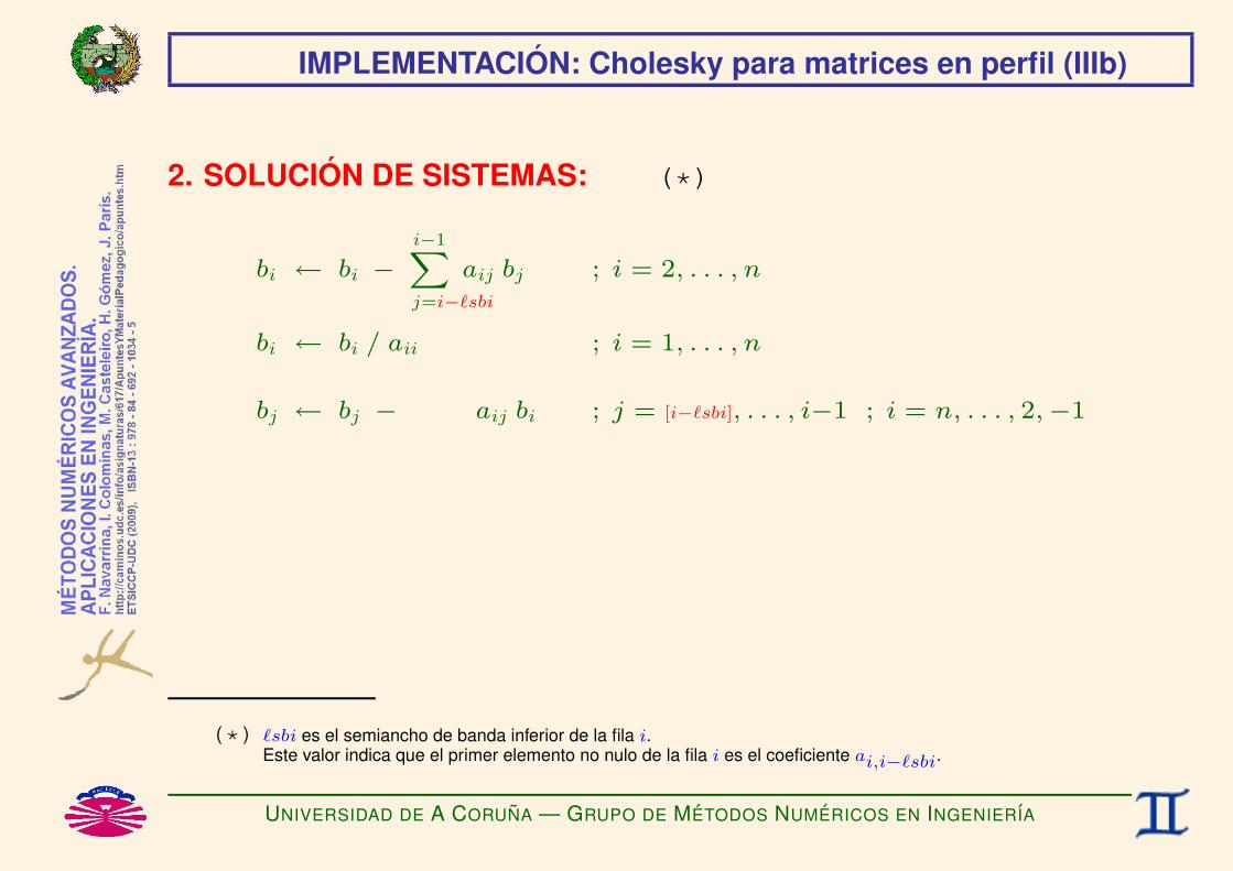
2. SOLUCION DE SISTEMAS: (*)
bi ← bi −i−1Xj=i−`(i)
aij bj ; i = 2, . . . , n
bi ← bi / aii ; i = 1, . . . , n
bj ← bj − aij bi ; j = [i−`(i)], . . . , i−1 ; i = n, . . . , 2,−1
(*) `(i) es el semiancho de banda inferior de la fila i.Este valor indica que el primer elemento no nulo de la fila i es el coeficiente ai,i−`(i).
UNIVERSIDAD DE A CORUNA — GRUPO DE METODOS NUMERICOS EN INGENIERIA

CONDICIONES DE VINCULACION [coacciones] (I)
Sea el sistema
a11 a12 a13 · · · a1v · · · a1n
a21 a22 a23 · · · a2v · · · a2n
a31 a32 a33 · · · a3v · · · a3n... ... ... . . . ... ...av1 av2 av3 · · · avv · · · avn... ... ... ... . . . ...an1 an2 an3 · · · anv · · · ann
x1
x2
x3...xv...xn
=
b1
b2
b3...bv...bn
+
000...rv...0
,
con la coaccion adicional
xv = pv , donde
v = GRADO DE LIBERTAD (GDL) COACCIONADO,
pv = VALOR PRESCRITO (conocido),
rv = REACCION (desconocida).
UNIVERSIDAD DE A CORUNA — GRUPO DE METODOS NUMERICOS EN INGENIERIA

CONDICIONES DE VINCULACION [coacciones] (II)
El planteamiento anterior puede reescribirse en la forma
a11 a12 a13 · · · 0 · · · a1n
a21 a22 a23 · · · 0 · · · a2n
a31 a32 a33 · · · 0 · · · a3n... ... ... . . . ... ...0 0 0 · · · 1 · · · 0... ... ... ... . . . ...
an1 an2 an3 · · · 0 · · · ann
x1
x2
x3...xv...xn
=
b1−a1v pv
b2−a2v pv
b3−a3v pv
...pv
...bn−anv pv
,
con la ecuacion adicional
rv = [ av1 av2 av3 · · · avv · · · avn ]
x1
x2
x3...xv...xn
− bv,
que se utiliza una vez resuelto el sistema anterior.
UNIVERSIDAD DE A CORUNA — GRUPO DE METODOS NUMERICOS EN INGENIERIA

CONDICIONES DE VINCULACION [coacciones] (III)
TRATAMIENTO DE LAS CONDICIONES DE VINCULACION [coacciones]
Dado el sistema Ae x = b + r, con algunas xv = pv, se procede de la siguiente manera:
1) Al factorizar se ignoran filas y columnas correspondientes a GDL prescritos (v).2) Las columnas correspondientes a GDL prescritos pasan restando a los terminos
independientes multiplicadas por los valores prescritos (−aiv pv ).
3) Las filas correspondientes a GDL prescritos (avj) se usan a posteriori para calcularlas reacciones ( rv ).
Luego, los datos almacenados en filas y columnas correspondientes a GDL prescritos
♣ no se alteran durante la factorizacion y♥ se pueden utilizar para resolver multiples sistemas con la misma matriz y distintos
B terminos independientes oB valores prescritos. (*)
(*) ¡OJO!: pueden cambiarse los valores prescritos (pv), pero no pueden cambiarse los GDL prescritos (v).
UNIVERSIDAD DE A CORUNA — GRUPO DE METODOS NUMERICOS EN INGENIERIA

IMPLEMENTACION: Cholesky para matrices en perfil (Ia)
CODIFICACION DEL ALMACENAMIENTO (§)
A˜ =
a11
∗ ∗0 ∗ ∗ SIM.0 ∗ · · · ∗0 0 ∗ · · · ∗0 ∗ · · · · · · · · · ∗0 0 0 ai,i−`sbi · · · ai,i−1 aii −→ fila i
0 0 ∗ · · · · · · · · · · · · ∗0 0 0 0 ∗ · · · · · · · · · ann
(§) PARTE TRIANGULAR SUPERIOR EN PERFIL POR COLUMNAS⇐⇒ PARTE TRIANGULAR INFERIOR EN PERFIL POR FILAS.
UNIVERSIDAD DE A CORUNA — GRUPO DE METODOS NUMERICOS EN INGENIERIA

IMPLEMENTACION: Cholesky para matrices en perfil (Ib)
ALMACENAMIENTO EN PERFIL (*)A˜ se almacena en v = [a11, · · · , ai,i−`sbi, · · · , · · · , ai,i−1, aii, · · · , · · · , ann]
aij vk, con k = lpij ≡ puntero del coeficiente aij.
Si lp(i) ≡ puntero del coeficiente aii, entonces:
8>>>><>>>>:lpii = |lp(i)| ≡ puntero de aii, (∗∗)
lsbi = lpii − (|lp(i − 1)| + 1) ≡ semiancho de banda inferior de la fila i, (∗∗)
lpiØ = lpii − i,
lpij = lpiØ + j ≡ puntero de aij, con i − lsbi ≤ j ≤ i,
(*) Sistema de punteros y variables utilizado en la subrutina SLE$Solver_LDLt_CP().
(**) Se utilizan valores absolutos porque esta subrutina cambia los signos de los punteros de los GDL coaccionados.
UNIVERSIDAD DE A CORUNA — GRUPO DE METODOS NUMERICOS EN INGENIERIA
IMPLEMENTACION: Cholesky para matrices en perfil (II)
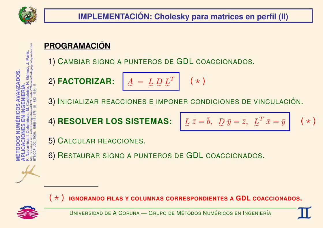
PROGRAMACION
1) CAMBIAR SIGNO A PUNTEROS DE GDL COACCIONADOS.
2) FACTORIZAR: A˜ = L˜ D˜ L˜T (*)
3) INICIALIZAR REACCIONES E IMPONER CONDICIONES DE VINCULACION.
4) RESOLVER LOS SISTEMAS: L˜ z = b, D˜ y = z, L˜T x = y (*)
5) CALCULAR REACCIONES.
6) RESTAURAR SIGNO A PUNTEROS DE GDL COACCIONADOS.
(*) IGNORANDO FILAS Y COLUMNAS CORRESPONDIENTES A GDL COACCIONADOS.
UNIVERSIDAD DE A CORUNA — GRUPO DE METODOS NUMERICOS EN INGENIERIA

IMPLEMENTACION: Cholesky para matrices en perfil (IIIa)
1. FACTORIZACION DE LA MATRIZ: (*)
DO k=2,n
aki ← aki −i−1Xj=maxi−`sbi,k−`sbk
aij akj ; i = [k−`sbk+1], . . . , k − 1
aki ← aki / aii ; i = [k−`sbk], . . . , k − 1
akk ← akk −k−1Xj=k−`sbk
akj ajj akj
ENDDO
(*) `sbi es el semiancho de banda inferior de la fila i.Este valor indica que el primer elemento no nulo de la fila i es el coeficiente ai,i−`sbi.
UNIVERSIDAD DE A CORUNA — GRUPO DE METODOS NUMERICOS EN INGENIERIA
IMPLEMENTACION: Cholesky para matrices en perfil (IIIb)
2. SOLUCION DE SISTEMAS: (*)
bi ← bi −i−1Xj=i−`sbi
aij bj ; i = 2, . . . , n
bi ← bi / aii ; i = 1, . . . , n
bj ← bj − aij bi ; j = [i−`sbi], . . . , i−1 ; i = n, . . . , 2,−1
(*) `sbi es el semiancho de banda inferior de la fila i.Este valor indica que el primer elemento no nulo de la fila i es el coeficiente ai,i−`sbi.
UNIVERSIDAD DE A CORUNA — GRUPO DE METODOS NUMERICOS EN INGENIERIA


CALCULO MATRICIALDE CIRCUITOS DE CORRIENTE CONTINUA
F. Navarrina, I. Colominas, M. Casteleiro, H. Gomez, J. Parıs
GMNI — GRUPO DE METODOS NUMERICOS EN INGENIERIA
Departamento de Metodos Matematicos y de RepresentacionEscuela Tecnica Superior de Ingenieros de Caminos, Canales y Puertos
Universidad de A Coruna, Espana
e-mail: [email protected] web: http://caminos.udc.es/gmni
UNIVERSIDAD DE A CORUNA — GRUPO DE METODOS NUMERICOS EN INGENIERIA

INDICE
I Ejemplo
I Ecuaciones Constitutivas y de Compatibilidad
I Ecuaciones de Equilibrio
I Numeracion Global: Matriz de Conectividad
I Equilibrio Elemental en Numeracion Global
I Equilibrio Global
I La Matriz de Rigidez es Semi-Definida Positiva
I La Matriz de Rigidez Coaccionada es Definida Positiva
UNIVERSIDAD DE A CORUNA — GRUPO DE METODOS NUMERICOS EN INGENIERIA

Ejemplo (I)
DATOS (*):
Materiales:
Cable Resistencia (Ω)
1, 4 484.00
2, 3 242.00
5 1210.00
GDL Coaccionados:
E = 220 V (generador)
V0 = 0 V (potencial de tierra)
Casos de Carga:
I) F2 = 0.00 AII) F2 = 2.00 A
(*) Vease la codificacion de este problema en el archivo ejemplo.dat.
UNIVERSIDAD DE A CORUNA — GRUPO DE METODOS NUMERICOS EN INGENIERIA

Ejemplo (II)
Algunas variables importantes. . .
npoin=4 (4 nodos)
nelem=5 (5 elementos→ conductores)
nnode=2 (2 nodos por elemento)
nprop=1 (1 propiedad por material→ resistencia electrica)
. . .
NOTA: El sentido de la intensidad en cada elemento se elige de forma arbitraria.
(*) Vease la codificacion de este problema en el archivo ejemplo.dat.
UNIVERSIDAD DE A CORUNA — GRUPO DE METODOS NUMERICOS EN INGENIERIA

Ecuaciones Constitutivas y de Compatibilidad (I)
Vector de desplazamientos (potenciales) elementales:
ue =
u1,e
u2,e
.
UNIVERSIDAD DE A CORUNA — GRUPO DE METODOS NUMERICOS EN INGENIERIA

Ecuaciones Constitutivas y de Compatibilidad (II)
Vector de deformaciones (gradientes de potencial) elementales:
εe = u2,e − u1,e .
ECUACION DE COMPATIBILIDAD:
εe = B˜ eue, B˜ e = [−1 +1 ] .
UNIVERSIDAD DE A CORUNA — GRUPO DE METODOS NUMERICOS EN INGENIERIA

Ecuaciones Constitutivas y de Compatibilidad (III)
Vector de tensiones (intensidades circulantes) elementales:
σe = Ie .
ECUACION CONSTITUTIVA (Ley de Ohm):
σe = D˜ eεe, D˜ e = [ 1Re
] .
UNIVERSIDAD DE A CORUNA — GRUPO DE METODOS NUMERICOS EN INGENIERIA

Ecuaciones Constitutivas y de Compatibilidad (IV)
NOTA IMPORTANTE:
Observese que en esta formulacion, el signo de la intensidad es elcontrario del habitual (*).
Lo anterior debera tenerse en cuenta tanto al introducir los datos comoal interpretar los resultados.
(*) Se ha hecho ası para que la matriz De e sea definitiva positiva, como sucede con lasrestantes formulaciones que se presentan durante este curso.
UNIVERSIDAD DE A CORUNA — GRUPO DE METODOS NUMERICOS EN INGENIERIA

Ecuaciones de Equilibrio (I)
Vector de fuerzas (intensidades salientes) elementales:
fe =
I1,e
I2,e
=−Ie
+Ie
.
ECUACION DE EQUILIBRIO:
fe = B˜Te σe, B˜T
e =[−1+1
].
UNIVERSIDAD DE A CORUNA — GRUPO DE METODOS NUMERICOS EN INGENIERIA

Ecuaciones de Equilibrio (II)
Luego,
εe = B˜ eue
σe = D˜ eεe
fe = B˜Te σe
=⇒
σe = D˜ e
(B˜ eue
)=
S˜e︷ ︸︸ ︷(D˜ eB˜ e
)ue,
fe = B˜Te
(S˜eue
)=(B˜T
e S˜e
)︸ ︷︷ ︸K˜ e
ue.
Matriz de Rigidez de Elemento:
K˜ e = B˜Te D˜ eB˜ e =
[+ 1
Re− 1
Re
− 1Re
+ 1Re
].
ECUACION ELEMENTAL (Constitutiva+Compatibilidad+Equilibrio):
K˜ eue = fe.
UNIVERSIDAD DE A CORUNA — GRUPO DE METODOS NUMERICOS EN INGENIERIA

Numeracion Global: Matriz de Conectividad (I)
Vector de Desplazamientos (Potenciales) Nodales:
u =
u1
u2
u3
u4
.
CAMBIO DE NUMERACION LOCAL A NUMERACION GLOBAL
Matriz de Conectividad: lnods(nnode,nelem)
ipoin=lnods(inode,ielem) =⇒
8>><>>:ielem = elemento
inode = numeracion local 1,2 del nodo
ipoin = numeracion global del nodo
UNIVERSIDAD DE A CORUNA — GRUPO DE METODOS NUMERICOS EN INGENIERIA

Numeracion Global: Matriz de Conectividad (II)
En el ejemplo que estamos utilizando (*) . . .
lnods(1,1)=1 lnods(2,1)=2
lnods(1,2)=2 lnods(2,2)=3
lnods(1,3)=1 lnods(2,3)=4
lnods(1,4)=3 lnods(2,4)=4
lnods(1,5)=3 lnods(2,5)=1
(*) Vease la codificacion de este problema en el archivo ejemplo.dat.
UNIVERSIDAD DE A CORUNA — GRUPO DE METODOS NUMERICOS EN INGENIERIA

Equilibrio Elemental en Numeracion Global (I)
ielem=1
K˜ 1u1 = f1 =⇒ K˜ 1u = f1.
[+ 1
R1− 1
R1
− 1R1
+ 1R1
]u1,1
u2,1
=
I1,1
I2,1
=⇒
+ 1
R1− 1
R10 0
− 1R1
+ 1R1
0 00 0 0 00 0 0 0
u1
u2
u3
u4
=
I1,1
I2,1
00
.
UNIVERSIDAD DE A CORUNA — GRUPO DE METODOS NUMERICOS EN INGENIERIA
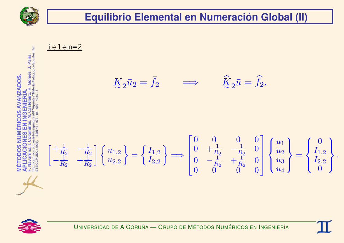
Equilibrio Elemental en Numeracion Global (II)
ielem=2
K˜ 2u2 = f2 =⇒ K˜ 2u = f2.
[+ 1
R2− 1
R2
− 1R2
+ 1R2
]u1,2
u2,2
=
I1,2
I2,2
=⇒
0 0 0 00 + 1
R2− 1
R20
0 − 1R2
+ 1R2
00 0 0 0
u1
u2
u3
u4
=
0
I1,2
I2,2
0
.
UNIVERSIDAD DE A CORUNA — GRUPO DE METODOS NUMERICOS EN INGENIERIA

Equilibrio Elemental en Numeracion Global (III)
ielem=3
K˜ 3u3 = f3 =⇒ K˜ 3u = f3.
[+ 1
R3− 1
R3
− 1R3
+ 1R3
]u1,3
u2,3
=
I1,3
I2,3
=⇒
+ 1
R30 0 − 1
R30 0 0 00 0 0 0
− 1R3
0 0 + 1R3
u1
u2
u3
u4
=
I1,3
00
I2,3
.
UNIVERSIDAD DE A CORUNA — GRUPO DE METODOS NUMERICOS EN INGENIERIA

Equilibrio Elemental en Numeracion Global (IV)
ielem=4
K˜ 4u4 = f4 =⇒ K˜ 4u = f4.
[+ 1
R4− 1
R4
− 1R4
+ 1R4
]u1,4
u2,4
=
I1,4
I2,4
=⇒
0 0 0 00 0 0 00 0 + 1
R4− 1
R4
0 0 − 1R4
+ 1R4
u1
u2
u3
u4
=
00
I1,4
I2,4
.
UNIVERSIDAD DE A CORUNA — GRUPO DE METODOS NUMERICOS EN INGENIERIA

Equilibrio Elemental en Numeracion Global (V)
ielem=5
K˜ 5u5 = f5 =⇒ K˜ 5u = f5.
[+ 1
R5− 1
R5
− 1R5
+ 1R5
]u1,5
u2,5
=
I1,5
I2,5
=⇒
+ 1
R50 − 1
R50
0 0 0 0− 1
R50 + 1
R50
0 0 0 0
u1
u2
u3
u4
=
I2,5
0I1,5
0
.
UNIVERSIDAD DE A CORUNA — GRUPO DE METODOS NUMERICOS EN INGENIERIA

Equilibrio Global (I)
El equilibrio de cada nodoesta gobernado por laLEY DE KIRCHOFF:
La Intensidad saliente decada nodo es igual a lasuma de las aportaciones(intensidades salientes)de todas las resistenciasque confluyen en el.
UNIVERSIDAD DE A CORUNA — GRUPO DE METODOS NUMERICOS EN INGENIERIA
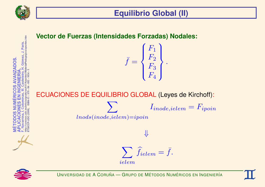
Equilibrio Global (II)
Vector de Fuerzas (Intensidades Forzadas) Nodales:
f =
F1
F2
F3
F4
.
ECUACIONES DE EQUILIBRIO GLOBAL (Leyes de Kirchoff):∑lnods(inode,ielem)=ipoin
Iinode,ielem = Fipoin
⇓∑ielem
fielem = f .
UNIVERSIDAD DE A CORUNA — GRUPO DE METODOS NUMERICOS EN INGENIERIA

Equilibrio Global (III)
Las ecuaciones de equilibrio global pueden reescribirse en la forma matricial
K˜ ielemu = fielem∑ielem
fielem = f
=⇒
(∑ielem
K˜ ielem
)︸ ︷︷ ︸
K˜u = f .
Matriz de Rigidez Global:
K˜ =
(∑ielem
K˜ ielem
)︸ ︷︷ ︸
ENSAMBLAJE DE LAS Ke ielem
.
ECUACION DE EQUILIBRIO GLOBAL:
K˜ u = f .
UNIVERSIDAD DE A CORUNA — GRUPO DE METODOS NUMERICOS EN INGENIERIA

Equilibrio Global (IV)
Luego, el sistema que hay que resolver es el siguiente:2666666664
“1
R1+ 1
R3+ 1
R5
”− 1
R1− 1
R5− 1
R3
− 1R1
“1
R1+ 1
R2
”− 1
R20
− 1R5
− 1R2
“1
R2+ 1
R4+ 1
R5
”− 1
R4
− 1R3
0 − 1R4
“1
R3+ 1
R4
”
3777777775
8>>>>>>><>>>>>>>:
u1
u2
u3
u4
9>>>>>>>=>>>>>>>;=
8>>>>>>><>>>>>>>:
0
F2
0
0
9>>>>>>>=>>>>>>>;+
8>>>>>>><>>>>>>>:
0
0
F R3
F R4
9>>>>>>>=>>>>>>>;m
K˜ u = f + R, K˜ = K˜ T ,
con las condiciones de vinculacion
u3 = Eu4 = 0
ff⇐⇒ uV = pV ,
donde V es cada uno de los grados de libertad coaccionados.
UNIVERSIDAD DE A CORUNA — GRUPO DE METODOS NUMERICOS EN INGENIERIA

La Matriz de Rigidez es Semi-DEF. POS.
uTK˜ u =∑
e
uT K˜ eu con K˜ =∑
e
K˜ e
=∑
e
uTe K˜ eue donde K˜ e = B˜T
e D˜ eB˜ e
=∑
e
uTe
(B˜T
e D˜ eB˜ e
)ue
=∑
e
(B˜ eue)T
D˜ e (B˜ eue)
=∑
e
εTe D˜ eεe con εe = B˜ eue
≥ 0, pues D˜ e = [1/Re] es SEMI-DEF +.
Luego uTK˜ u ≥ 0 ∀u =⇒ K˜ es SEMI-DEFINIDA POSITIVA.
UNIVERSIDAD DE A CORUNA — GRUPO DE METODOS NUMERICOS EN INGENIERIA

La Matriz Coaccionada es DEF. POS. (I)
Sea K˜ V la matriz que se obtiene al ignorar las filas y columnas de la matrizK˜ correspondientes a g.d.l. coaccionados.
K˜ =
kv,v
, K˜ V =
.
UNIVERSIDAD DE A CORUNA — GRUPO DE METODOS NUMERICOS EN INGENIERIA

La Matriz Coaccionada es DEF. POS. (II)
Sea u 6= 0 un vector en el que todos los componentes correspondientes ag.d.l. coaccionados son nulos.
Sea uV 6= 0 el vector que se obtiene al ignorar las filas del vector ucorrespondientes a g.d.l. coaccionados.
u =
0
, uV =
.
En estas condiciones uTV K˜ V uV = uTK˜ u, pues. . .
UNIVERSIDAD DE A CORUNA — GRUPO DE METODOS NUMERICOS EN INGENIERIA

La Matriz Coaccionada es DEF. POS. (III)
uTV K˜ V uV = [ ]
,
uTK˜ u = [ 0 ]
kv,v
0
.
UNIVERSIDAD DE A CORUNA — GRUPO DE METODOS NUMERICOS EN INGENIERIA
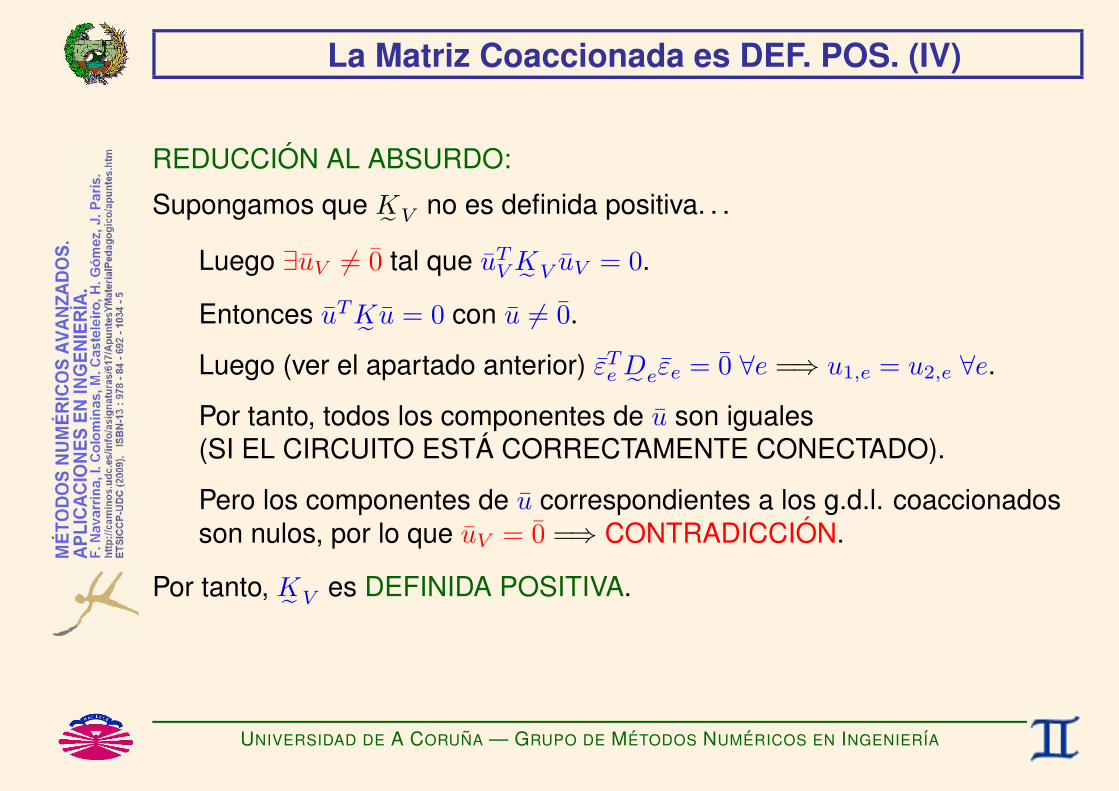
La Matriz Coaccionada es DEF. POS. (IV)
REDUCCION AL ABSURDO:
Supongamos que K˜ V no es definida positiva. . .
Luego ∃uV 6= 0 tal que uTV K˜ V uV = 0.
Entonces uTK˜ u = 0 con u 6= 0.
Luego (ver el apartado anterior) εTe D˜ eεe = 0 ∀e =⇒ u1,e = u2,e ∀e.
Por tanto, todos los componentes de u son iguales(SI EL CIRCUITO ESTA CORRECTAMENTE CONECTADO).
Pero los componentes de u correspondientes a los g.d.l. coaccionadosson nulos, por lo que uV = 0 =⇒ CONTRADICCION.
Por tanto, K˜ V es DEFINIDA POSITIVA.
UNIVERSIDAD DE A CORUNA — GRUPO DE METODOS NUMERICOS EN INGENIERIA
CALCULO MATRICIALDE ESTRUCTURAS DE BARRAS
(Articuladas 2D-3D)F. Navarrina, I. Colominas, M. Casteleiro, H. Gomez, J. Parıs
GMNI — GRUPO DE METODOS NUMERICOS EN INGENIERIA
Departamento de Metodos Matematicos y de RepresentacionEscuela Tecnica Superior de Ingenieros de Caminos, Canales y Puertos
Universidad de A Coruna, Espana
e-mail: [email protected] web: http://caminos.udc.es/gmni
UNIVERSIDAD DE A CORUNA — GRUPO DE METODOS NUMERICOS EN INGENIERIA

INDICE
I Ejemplos
I Ejes Locales y Globales
I Ecuaciones Constitutivas y de Compatibilidad
I Ecuaciones de Equilibrio
I Numeracion Global: Matriz de Conectividad
I Equilibrio Elemental en Numeracion Global
I Equilibrio Global
I La Matriz de Rigidez es Semi-Definida Positiva
I La Matriz de Rigidez Coaccionada es Definida Positiva
UNIVERSIDAD DE A CORUNA — GRUPO DE METODOS NUMERICOS EN INGENIERIA

Ejemplos (I)
Veanse los ejemplos siguientes:
Estructura Articulada 2D• Descripcion: ejemplo2.pdf
• Codificacion: ejemplo2.dat
Estructura Articulada 3D• Descripcion: ejemplo3.pdf
• Codificacion: ejemplo3.dat
UNIVERSIDAD DE A CORUNA — GRUPO DE METODOS NUMERICOS EN INGENIERIA

Ejemplo (II)
Algunas variables importantes. . .
npoin=* (numero de nodos)
ndime=* (numero de coordenadas por nodo: 2 en 2D, 3 en 3D)
nelem=* (numero de elementos → barras)
nnode=2 (2 nodos por elemento)
ndofn=* (NUMERO DE GDL POR NODO: 2 en 2D, 3 en 3D)
nprop=1 (numero de propiedades por material → EA)
. . .
(*) Veanse ejemplos de codificacion de este tipo de problemas en los archivosejemplo2.dat y ejemplo3.dat.
UNIVERSIDAD DE A CORUNA — GRUPO DE METODOS NUMERICOS EN INGENIERIA

Ejes Locales y Globales
Cambio de Base
r =
Q˜Te︷ ︸︸ ︷ cosα ∗ ∗cos β ∗ ∗cos γ ∗ ∗
r′,r′ =
cosα cos β cos γ
∗ ∗ ∗∗ ∗ ∗
︸ ︷︷ ︸
Q˜ er,
pues(Q˜ e)−1
= Q˜Te .
UNIVERSIDAD DE A CORUNA — GRUPO DE METODOS NUMERICOS EN INGENIERIA

Ecuaciones Constitutivas y de Compatibilidad (I)
Vector de desplazamientoselementales en ejes globales:
ue =
u1,e
u2,e
u1,e =
u1,e
v1,e
w1,e
, u2,e =
u2,e
v2,e
w2,e
.
UNIVERSIDAD DE A CORUNA — GRUPO DE METODOS NUMERICOS EN INGENIERIA
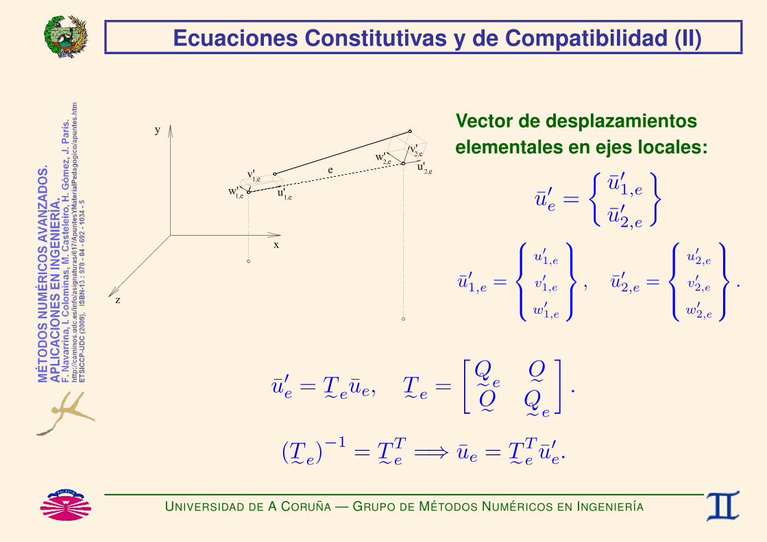
Ecuaciones Constitutivas y de Compatibilidad (II)
Vector de desplazamientoselementales en ejes locales:
u′e =
u′1,e
u′2,e
u′1,e =
u′1,e
v′1,e
w′1,e
, u′2,e =
u′2,e
v′2,e
w′2,e
.
u′e = T˜eue, T˜e =[
Q˜ eO˜O˜ Q˜ e
].
(T˜e)−1 = T˜T
e =⇒ ue = T˜Te u′e.
UNIVERSIDAD DE A CORUNA — GRUPO DE METODOS NUMERICOS EN INGENIERIA

Ecuaciones Constitutivas y de Compatibilidad (III)
Vector de deformacioneselementales:
εe = ∆Le ,
∆Le = u′2,e − u′1,e.
UNIVERSIDAD DE A CORUNA — GRUPO DE METODOS NUMERICOS EN INGENIERIA

Ecuaciones Constitutivas y de Compatibilidad (IV)
Relacion desplazamientos—deformaciones:
εe = E˜ eu′e, E˜ e = [−1 0 0 +1 0 0 ] .
Luego,
u′e = T˜eue
εe = E˜ eu′e
=⇒ εe = E˜ e
(T˜eue
)=
B˜ e︷ ︸︸ ︷(E˜ eT˜e
)ue.
ECUACION DE COMPATIBILIDAD:
εe = B˜ eue, B˜ e = [− cos α − cos β − cos γ + cos α + cos β + cos γ ].
UNIVERSIDAD DE A CORUNA — GRUPO DE METODOS NUMERICOS EN INGENIERIA

Ecuaciones Constitutivas y de Compatibilidad (V)
Vector de tensioneselementales:
σe = Ne ,
Ne =(
EAe
Le
)∆Le.
ECUACION CONSTITUTIVA:
σe = D˜ eεe, D˜ e = [ EAeLe
] .
UNIVERSIDAD DE A CORUNA — GRUPO DE METODOS NUMERICOS EN INGENIERIA

Ecuaciones de Equilibrio (I)
Vector de fuerzaselementales en ejes globales:
fe =
f1,e
f2,e
f1,e =
fx1,e
fy1,e
fz1,e
, f2,e =
fx2,e
fy2,e
fz2,e
.
UNIVERSIDAD DE A CORUNA — GRUPO DE METODOS NUMERICOS EN INGENIERIA

Ecuaciones de Equilibrio (II)
Vector de fuerzaselementales en ejes locales:
f ′e =
f ′1,e
f ′2,e
f ′1,e =
fx′1,e
fy′1,e
fz′1,e
, f ′2,e =
fx′2,e
fy′2,e
fz′2,e
.
f ′e = T˜efe, T˜e =[
Q˜ eO˜O˜ Q˜ e
].
(T˜e)−1 = T˜T
e =⇒ fe = T˜Te f ′e.
UNIVERSIDAD DE A CORUNA — GRUPO DE METODOS NUMERICOS EN INGENIERIA

Ecuaciones de Equilibrio (III)
Relacion tensiones—fuerzas elementales:
f ′e = E˜Te σe, E˜T
e =
−100
+100
.
Luego,
f ′e = E˜Te σe
fe = T˜Te f ′e
=⇒ fe = T˜T
e
(E˜T
e σe
)=(T˜T
e E˜Te
)σe =
(E˜ eT˜e
)T︸ ︷︷ ︸B˜ T
e
σe.
ECUACION DE EQUILIBRIO
fe = B˜Te σe, B˜ e = [− cos α − cos β − cos γ + cos α + cos β + cos γ ].
UNIVERSIDAD DE A CORUNA — GRUPO DE METODOS NUMERICOS EN INGENIERIA
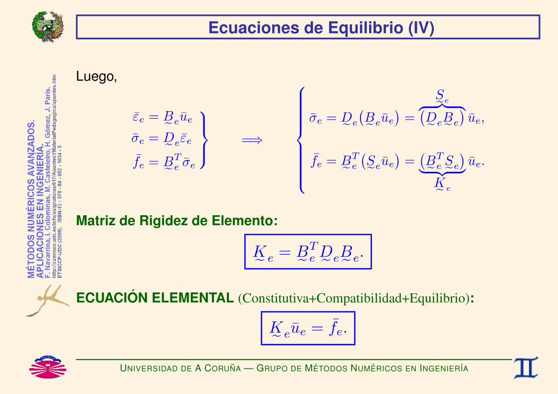
Ecuaciones de Equilibrio (IV)
Luego,
εe = B˜ eue
σe = D˜ eεe
fe = B˜Te σe
=⇒
σe = D˜ e
(B˜ eue
)=
S˜e︷ ︸︸ ︷(D˜ eB˜ e
)ue,
fe = B˜Te
(S˜eue
)=(B˜T
e S˜e
)︸ ︷︷ ︸K˜ e
ue.
Matriz de Rigidez de Elemento:
K˜ e = B˜Te D˜ eB˜ e.
ECUACION ELEMENTAL (Constitutiva+Compatibilidad+Equilibrio):
K˜ eue = fe.
UNIVERSIDAD DE A CORUNA — GRUPO DE METODOS NUMERICOS EN INGENIERIA

Numeracion Global: Matriz de Conectividad
Vector de Desplazamientos Nodales:
u =
...
uipoin
...
, uipoin =
uipoin
vipoin
wipoin
, ipoin = 1, . . . , npoin.
CAMBIO DE NUMERACION LOCAL A NUMERACION GLOBAL
Matriz de Conectividad: lnods(nnode,nelem) (*)
ipoin=lnods(inode,ielem) =⇒
8>><>>:ielem = elemento
inode = numeracion local 1,2 del nodo
ipoin = numeracion global del nodo
(*) Veanse ejemplos de codificacion de este tipo de problemas en los archivosejemplo2.dat y ejemplo3.dat.
UNIVERSIDAD DE A CORUNA — GRUPO DE METODOS NUMERICOS EN INGENIERIA
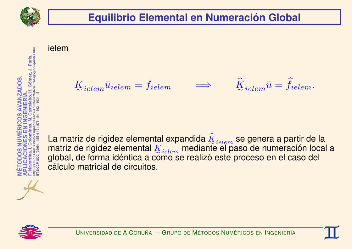
Equilibrio Elemental en Numeracion Global
ielem
K˜ ielemuielem = fielem =⇒ K˜ ielemu = fielem.
La matriz de rigidez elemental expandida K˜ ielem se genera a partir de lamatriz de rigidez elemental K˜ ielem mediante el paso de numeracion local aglobal, de forma identica a como se realizo este proceso en el caso delcalculo matricial de circuitos.
UNIVERSIDAD DE A CORUNA — GRUPO DE METODOS NUMERICOS EN INGENIERIA

Equilibrio Global (I)
El equilibrio de cada nodo estagobernado por la
LEY DE NEWTON:
La fuerza externa aplicada a cadanodo es igual a la suma de lasfuerzas elementales de todas lasbarras que confluyen en el.
UNIVERSIDAD DE A CORUNA — GRUPO DE METODOS NUMERICOS EN INGENIERIA

Equilibrio Global (II)
Vector de Fuerzas Nodales:
f =
...
Fipoin
...
, Fipoin =
F x
ipoin
Fyipoin
F zipoin
, ipoin = 1, . . . , npoin.
ECUACIONES DE EQUILIBRIO GLOBAL (Leyes de Newton):∑lnods(inode,ielem)=ipoin
finode,ielem = Fipoin
⇓∑ielem
fielem = f .
UNIVERSIDAD DE A CORUNA — GRUPO DE METODOS NUMERICOS EN INGENIERIA
Equilibrio Global (III)
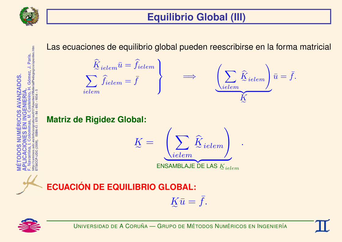
Las ecuaciones de equilibrio global pueden reescribirse en la forma matricial
K˜ ielemu = fielem∑ielem
fielem = f
=⇒
(∑ielem
K˜ ielem
)︸ ︷︷ ︸
K˜u = f .
Matriz de Rigidez Global:
K˜ =
(∑ielem
K˜ ielem
)︸ ︷︷ ︸
ENSAMBLAJE DE LAS Ke ielem
.
ECUACION DE EQUILIBRIO GLOBAL:
K˜ u = f .
UNIVERSIDAD DE A CORUNA — GRUPO DE METODOS NUMERICOS EN INGENIERIA
Equilibrio Global (IV)
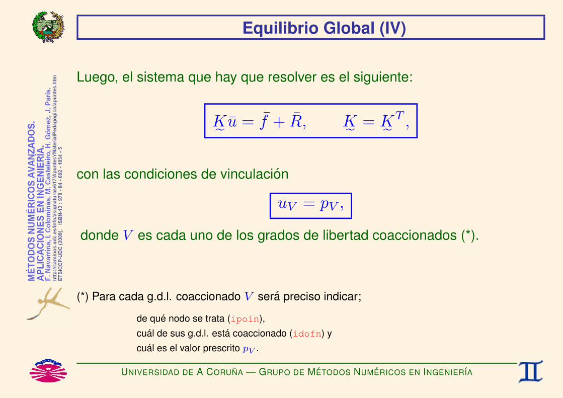
Luego, el sistema que hay que resolver es el siguiente:
K˜ u = f + R, K˜ = K˜ T ,
con las condiciones de vinculacion
uV = pV ,
donde V es cada uno de los grados de libertad coaccionados (*).
(*) Para cada g.d.l. coaccionado V sera preciso indicar;
de que nodo se trata (ipoin),cual de sus g.d.l. esta coaccionado (idofn) ycual es el valor prescrito pV .
UNIVERSIDAD DE A CORUNA — GRUPO DE METODOS NUMERICOS EN INGENIERIA
Equilibrio Global (V)
NOTA IMPORTANTE:
Observese que en estructuras articuladas 2D las componentes segun eleje z se anulan por lo que no es preciso tenerlas en cuenta, lo quepermite simplificar ligeramente la formulacion.
UNIVERSIDAD DE A CORUNA — GRUPO DE METODOS NUMERICOS EN INGENIERIA

La Matriz de Rigidez es Semi-DEF. POS.
uTK˜ u =∑
e
uT K˜ eu con K˜ =∑
e
K˜ e
=∑
e
uTe K˜ eue donde K˜ e = B˜T
e D˜ eB˜ e
=∑
e
uTe
(B˜T
e D˜ eB˜ e
)ue
=∑
e
(B˜ eue)T
D˜ e (B˜ eue)
=∑
e
εTe D˜ eεe con εe = B˜ eue
≥ 0, pues D˜ e = [EAe/Le] es SEMI-DEF +.
Luego uTK˜ u ≥ 0 ∀u =⇒ K˜ es SEMI-DEFINIDA POSITIVA.
UNIVERSIDAD DE A CORUNA — GRUPO DE METODOS NUMERICOS EN INGENIERIA

La Matriz Coaccionada es DEF. POS. (I)
Sea K˜ V la matriz que se obtiene al ignorar las filas y columnas de la matrizK˜ correspondientes a g.d.l. coaccionados.
K˜ =
kv,v
, K˜ V =
.
UNIVERSIDAD DE A CORUNA — GRUPO DE METODOS NUMERICOS EN INGENIERIA

La Matriz Coaccionada es DEF. POS. (II)
Sea u 6= 0 un vector en el que todos los componentes correspondientes ag.d.l. coaccionados son nulos.
Sea uV 6= 0 el vector que se obtiene al ignorar las filas del vector ucorrespondientes a g.d.l. coaccionados.
u =
0
, uV =
.
En estas condiciones uTV K˜ V uV = uTK˜ u, pues. . .
UNIVERSIDAD DE A CORUNA — GRUPO DE METODOS NUMERICOS EN INGENIERIA

La Matriz Coaccionada es DEF. POS. (III)
uTV K˜ V uV = [ ]
,
uTK˜ u = [ 0 ]
kv,v
0
.
UNIVERSIDAD DE A CORUNA — GRUPO DE METODOS NUMERICOS EN INGENIERIA

La Matriz Coaccionada es DEF. POS. (IV)
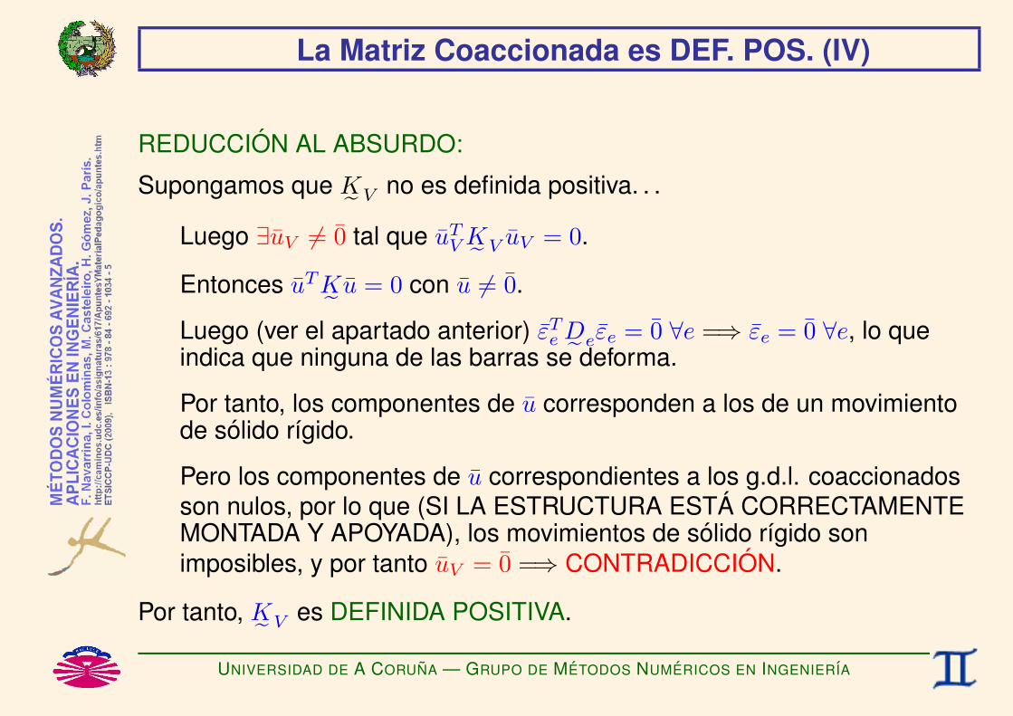
REDUCCION AL ABSURDO:
Supongamos que K˜ V no es definida positiva. . .
Luego ∃uV 6= 0 tal que uTV K˜ V uV = 0.
Entonces uTK˜ u = 0 con u 6= 0.
Luego (ver el apartado anterior) εTe D˜ eεe = 0 ∀e =⇒ εe = 0 ∀e, lo que
indica que ninguna de las barras se deforma.
Por tanto, los componentes de u corresponden a los de un movimientode solido rıgido.
Pero los componentes de u correspondientes a los g.d.l. coaccionadosson nulos, por lo que (SI LA ESTRUCTURA ESTA CORRECTAMENTEMONTADA Y APOYADA), los movimientos de solido rıgido sonimposibles, y por tanto uV = 0 =⇒ CONTRADICCION.
Por tanto, K˜ V es DEFINIDA POSITIVA.
UNIVERSIDAD DE A CORUNA — GRUPO DE METODOS NUMERICOS EN INGENIERIA

CALCULO MATRICIALDE ESTRUCTURAS DE BARRAS
(Reticuladas 2D)F. Navarrina, I. Colominas, M. Casteleiro, H. Gomez, J. Parıs
GMNI — GRUPO DE METODOS NUMERICOS EN INGENIERIA
Departamento de Metodos Matematicos y de RepresentacionEscuela Tecnica Superior de Ingenieros de Caminos, Canales y Puertos
Universidad de A Coruna, Espana
e-mail: [email protected] web: http://caminos.udc.es/gmni
UNIVERSIDAD DE A CORUNA — GRUPO DE METODOS NUMERICOS EN INGENIERIA

INDICE
I Ejemplos
I Ejes Locales y Globales
I Ecuaciones Constitutivas y de Compatibilidad
I Ecuaciones de Equilibrio
I Numeracion Global: Matriz de Conectividad
I Equilibrio Elemental en Numeracion Global
I Equilibrio Global
I La Matriz de Rigidez es Semi-Definida Positiva
I La Matriz de Rigidez Coaccionada es Definida Positiva
UNIVERSIDAD DE A CORUNA — GRUPO DE METODOS NUMERICOS EN INGENIERIA

Ejemplos (I)
Veanse los ejemplos siguientes:
Estructura Reticulada 2D• Descripcion: ejemplo4.pdf
• Codificacion: ejemplo4.dat
Gran Estructura Reticulada 2D (*)• Codificacion: ejsuper4.dat
ejsuper4renum.dat
(*) Sin renumerar (ejsuper4.dat) y con renumeracion (ejsuper4renum.dat).
UNIVERSIDAD DE A CORUNA — GRUPO DE METODOS NUMERICOS EN INGENIERIA
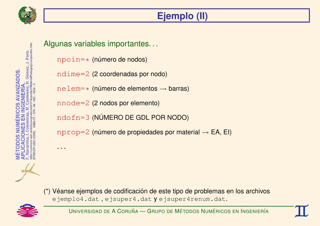
Ejemplo (II)
Algunas variables importantes. . .
npoin=* (numero de nodos)
ndime=2 (2 coordenadas por nodo)
nelem=* (numero de elementos → barras)
nnode=2 (2 nodos por elemento)
ndofn=3 (NUMERO DE GDL POR NODO)
nprop=2 (numero de propiedades por material → EA, EI)
. . .
(*) Veanse ejemplos de codificacion de este tipo de problemas en los archivosejemplo4.dat , ejsuper4.dat y ejsuper4renum.dat.
UNIVERSIDAD DE A CORUNA — GRUPO DE METODOS NUMERICOS EN INGENIERIA

Ejes Locales y Globales
Cambio de Base
r =
Q˜Te︷ ︸︸ ︷ cosα − cos β 0
cos β cosα 0
0 0 1
r′,r′ =
cosα cos β 0
− cos β cosα 0
0 0 1
︸ ︷︷ ︸
Q˜ er,
pues(Q˜ e)−1
= Q˜Te . (*)
(*) Ya que cos β = senα.
UNIVERSIDAD DE A CORUNA — GRUPO DE METODOS NUMERICOS EN INGENIERIA
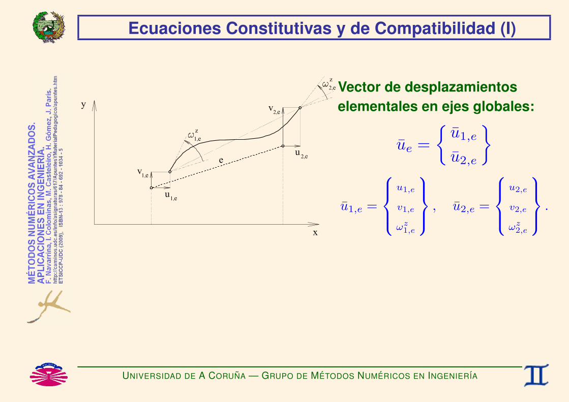
Ecuaciones Constitutivas y de Compatibilidad (I)
Vector de desplazamientoselementales en ejes globales:
ue =
u1,e
u2,e
u1,e =
u1,e
v1,e
ωz1,e
, u2,e =
u2,e
v2,e
ωz2,e
.
UNIVERSIDAD DE A CORUNA — GRUPO DE METODOS NUMERICOS EN INGENIERIA

Ecuaciones Constitutivas y de Compatibilidad (II)
Vector de desplazamientoselementales en ejes locales:
u′e =
u′1,e
u′2,e
u′1,e =
u′1,e
v′1,e
ωz′1,e
, u′2,e =
u′2,e
v′2,e
ωz′2,e
.
u′e = T˜eue, T˜e =[
Q˜ eO˜O˜ Q˜ e
].
(T˜e)−1 = T˜T
e =⇒ ue = T˜Te u′e.
UNIVERSIDAD DE A CORUNA — GRUPO DE METODOS NUMERICOS EN INGENIERIA

Ecuaciones Constitutivas y de Compatibilidad (III)
Vector de deformacioneselementales:
εe =
∆Le
∆ω1
∆ω2
,
con
∆Le = u′2,e − u
′1,e,
∆ω1 = ωz′1,e −
v′2,e − v′1,e
Le
,
∆ω2 = ωz′2,e −
v′2,e − v′1,e
Le
.
UNIVERSIDAD DE A CORUNA — GRUPO DE METODOS NUMERICOS EN INGENIERIA

Ecuaciones Constitutivas y de Compatibilidad (IV)
Relacion desplazamientos—deformaciones:
εe = E˜ eu′e, Ee e =
24−1 0 0 +1 0 00 + 1
Le+1 0 − 1
Le0
0 + 1Le
0 0 − 1Le
+1
35 .
Luego,
u′e = T˜eue
εe = E˜ eu′e
=⇒ εe = E˜ e
(T˜eue
)=
B˜ e︷ ︸︸ ︷(E˜ eT˜e
)ue.
ECUACION DE COMPATIBILIDAD:
εe = B˜ eue, B˜ e =24− cos α − cos β 0 + cos α + cos β 0−cos β
Le+cos α
Le+1 +cos β
Le−cos α
Le0
−cos βLe
+cos αLe
0 +cos βLe
−cos αLe
+1
35.
UNIVERSIDAD DE A CORUNA — GRUPO DE METODOS NUMERICOS EN INGENIERIA

Ecuaciones Constitutivas y de Compatibilidad (V)
Vector de tensioneselementales:
σe =
NM1
M2
,
con
N =EAe
Le∆Le, Q = −
M1 + M2Le
,M1M2
ff=
EIe
Le
»4 22 4
– ∆ω1∆ω2
ff
ECUACION CONSTITUTIVA:
σe = D˜ eεe, D˜ e =
EAeLe
0 00 4EIe
Le
2EIeLe
0 2EIeLe
4EIeLe
.
UNIVERSIDAD DE A CORUNA — GRUPO DE METODOS NUMERICOS EN INGENIERIA
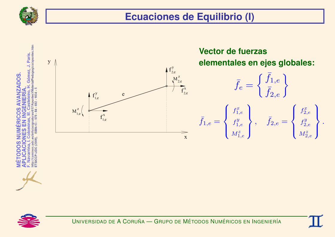
Ecuaciones de Equilibrio (I)
Vector de fuerzaselementales en ejes globales:
fe =
f1,e
f2,e
f1,e =
fx1,e
fy1,e
Mz1,e
, f2,e =
fx2,e
fy2,e
Mz2,e
.
UNIVERSIDAD DE A CORUNA — GRUPO DE METODOS NUMERICOS EN INGENIERIA

Ecuaciones de Equilibrio (II)
Vector de fuerzaselementales en ejes locales:
f ′e =
f ′1,e
f ′2,e
f ′1,e =
fx′1,e
fy′1,e
Mz′1,e
, f ′2,e =
fx′2,e
fy′2,e
Mz′2,e
.
f ′e = T˜efe, T˜e =[
Q˜ eO˜O˜ Q˜ e
].
(T˜e)−1 = T˜T
e =⇒ fe = T˜Te f ′e.
UNIVERSIDAD DE A CORUNA — GRUPO DE METODOS NUMERICOS EN INGENIERIA

Ecuaciones de Equilibrio (III)
Relacion tensiones—fuerzas elementales:
f ′e = E˜Te σe, E˜T
e =
−1 0 00 − 1
Le+ 1
Le0 +1 0
+1 0 00 − 1
Le− 1
Le0 0 1
.
Luego,
f ′e = E˜Te σe
fe = T˜Te f ′e
=⇒ fe = T˜T
e
(E˜T
e σe
)=(T˜T
e E˜Te
)σe =
(E˜ eT˜e
)T︸ ︷︷ ︸B˜ T
e
σe.
ECUACION DE EQUILIBRIO
fe = B˜Te σe, B˜ e =
24− cos α − cos β 0 + cos α + cos β 0−cos β
Le+cos α
Le+1 +cos β
Le−cos α
Le0
−cos βLe
+cos αLe
0 +cos βLe
−cos αLe
+1
35.
UNIVERSIDAD DE A CORUNA — GRUPO DE METODOS NUMERICOS EN INGENIERIA

Ecuaciones de Equilibrio (IV)
Luego,
εe = B˜ eue
σe = D˜ eεe
fe = B˜Te σe
=⇒
σe = D˜ e
(B˜ eue
)=
S˜e︷ ︸︸ ︷(D˜ eB˜ e
)ue,
fe = B˜Te
(S˜eue
)=(B˜T
e S˜e
)︸ ︷︷ ︸K˜ e
ue.
Matriz de Rigidez de Elemento:
K˜ e = B˜Te D˜ eB˜ e.
ECUACION ELEMENTAL (Constitutiva+Compatibilidad+Equilibrio):
K˜ eue = fe.
UNIVERSIDAD DE A CORUNA — GRUPO DE METODOS NUMERICOS EN INGENIERIA
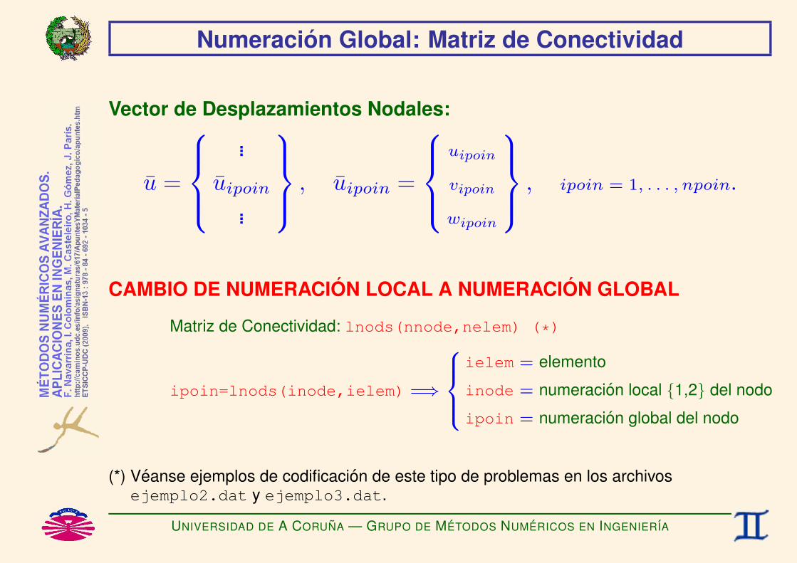
Numeracion Global: Matriz de Conectividad
Vector de Desplazamientos Nodales:
u =
...
uipoin
...
, uipoin =
uipoin
vipoin
wipoin
, ipoin = 1, . . . , npoin.
CAMBIO DE NUMERACION LOCAL A NUMERACION GLOBAL
Matriz de Conectividad: lnods(nnode,nelem) (*)
ipoin=lnods(inode,ielem) =⇒
8>><>>:ielem = elemento
inode = numeracion local 1,2 del nodo
ipoin = numeracion global del nodo
(*) Veanse ejemplos de codificacion de este tipo de problemas en los archivosejemplo2.dat y ejemplo3.dat.
UNIVERSIDAD DE A CORUNA — GRUPO DE METODOS NUMERICOS EN INGENIERIA

Equilibrio Elemental en Numeracion Global
ielem
K˜ ielemuielem = fielem =⇒ K˜ ielemu = fielem.
La matriz de rigidez elemental expandida K˜ ielem se genera a partir de lamatriz de rigidez elemental K˜ ielem mediante el paso de numeracion local aglobal, de forma identica a como se realizo este proceso en el caso delcalculo matricial de circuitos.
UNIVERSIDAD DE A CORUNA — GRUPO DE METODOS NUMERICOS EN INGENIERIA
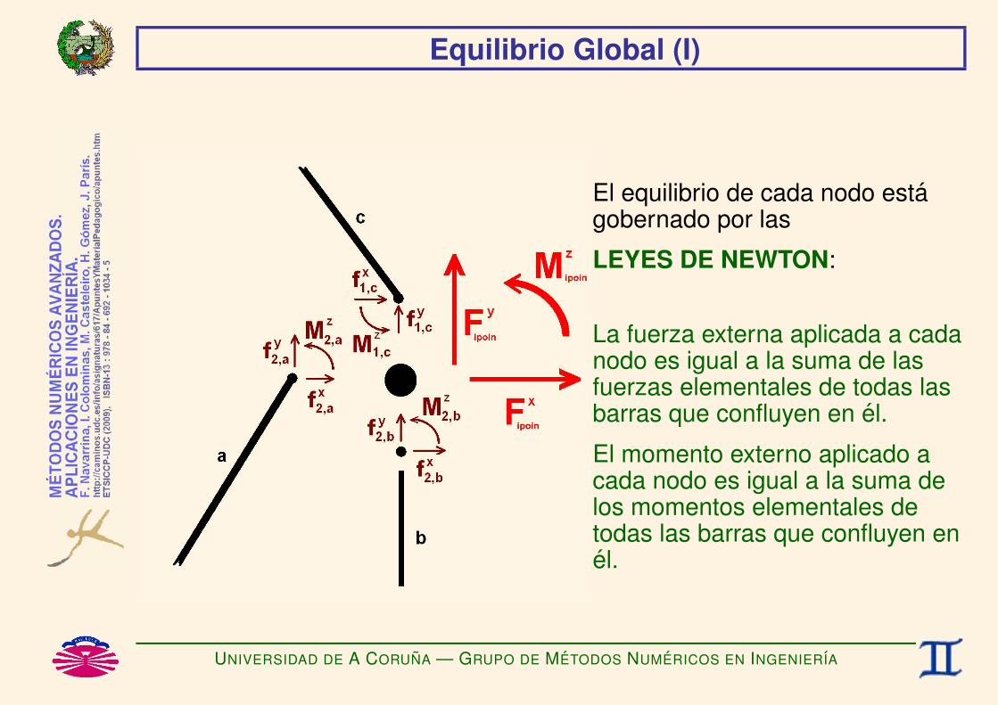
Equilibrio Global (I)
El equilibrio de cada nodo estagobernado por las
LEYES DE NEWTON:
La fuerza externa aplicada a cadanodo es igual a la suma de lasfuerzas elementales de todas lasbarras que confluyen en el.
El momento externo aplicado acada nodo es igual a la suma delos momentos elementales detodas las barras que confluyen enel.
UNIVERSIDAD DE A CORUNA — GRUPO DE METODOS NUMERICOS EN INGENIERIA

Equilibrio Global (II)
Vector de Fuerzas Nodales:
f =
...
Fipoin
...
, Fipoin =
F x
ipoin
Fyipoin
Mzipoin
, ipoin = 1, . . . , npoin.
ECUACIONES DE EQUILIBRIO GLOBAL (Leyes de Newton):∑lnods(inode,ielem)=ipoin
finode,ielem = Fipoin
⇓∑ielem
fielem = f .
UNIVERSIDAD DE A CORUNA — GRUPO DE METODOS NUMERICOS EN INGENIERIA

Equilibrio Global (III)
Las ecuaciones de equilibrio global pueden reescribirse en la forma matricial
K˜ ielemu = fielem∑ielem
fielem = f
=⇒
(∑ielem
K˜ ielem
)︸ ︷︷ ︸
K˜u = f .
Matriz de Rigidez Global:
K˜ =
(∑ielem
K˜ ielem
)︸ ︷︷ ︸
ENSAMBLAJE DE LAS Ke ielem
.
ECUACION DE EQUILIBRIO GLOBAL:
K˜ u = f .
UNIVERSIDAD DE A CORUNA — GRUPO DE METODOS NUMERICOS EN INGENIERIA

Equilibrio Global (IV)
Luego, el sistema que hay que resolver es el siguiente:
K˜ u = f + R, K˜ = K˜ T ,
con las condiciones de vinculacion
uV = pV ,
donde V es cada uno de los grados de libertad coaccionados (*).
(*) Para cada g.d.l. coaccionado V sera preciso indicar;
de que nodo se trata (ipoin),cual de sus g.d.l. esta coaccionado (idofn) ycual es el valor prescrito pV .
UNIVERSIDAD DE A CORUNA — GRUPO DE METODOS NUMERICOS EN INGENIERIA

La Matriz de Rigidez es Semi-DEF. POS.
uTK˜ u =∑
e
uT K˜ eu con K˜ =∑
e
K˜ e
=∑
e
uTe K˜ eue donde K˜ e = B˜T
e D˜ eB˜ e
=∑
e
uTe
(B˜T
e D˜ eB˜ e
)ue
=∑
e
(B˜ eue)T
D˜ e (B˜ eue)
=∑
e
εTe D˜ eεe con εe = B˜ eue
≥ 0, pues D˜ e = [. . .] es SEMI-DEF +.
Luego uTK˜ u ≥ 0 ∀u =⇒ K˜ es SEMI-DEFINIDA POSITIVA.
UNIVERSIDAD DE A CORUNA — GRUPO DE METODOS NUMERICOS EN INGENIERIA

La Matriz Coaccionada es DEF. POS. (I)
Sea K˜ V la matriz que se obtiene al ignorar las filas y columnas de la matrizK˜ correspondientes a g.d.l. coaccionados.
K˜ =
kv,v
, K˜ V =
.
UNIVERSIDAD DE A CORUNA — GRUPO DE METODOS NUMERICOS EN INGENIERIA

La Matriz Coaccionada es DEF. POS. (II)
Sea u 6= 0 un vector en el que todos los componentes correspondientes ag.d.l. coaccionados son nulos.
Sea uV 6= 0 el vector que se obtiene al ignorar las filas del vector ucorrespondientes a g.d.l. coaccionados.
u =
0
, uV =
.
En estas condiciones uTV K˜ V uV = uTK˜ u, pues. . .
UNIVERSIDAD DE A CORUNA — GRUPO DE METODOS NUMERICOS EN INGENIERIA

La Matriz Coaccionada es DEF. POS. (III)
uTV K˜ V uV = [ ]
,
uTK˜ u = [ 0 ]
kv,v
0
.
UNIVERSIDAD DE A CORUNA — GRUPO DE METODOS NUMERICOS EN INGENIERIA
La Matriz Coaccionada es DEF. POS. (IV)
REDUCCION AL ABSURDO:
Supongamos que K˜ V no es definida positiva. . .
Luego ∃uV 6= 0 tal que uTV K˜ V uV = 0.
Entonces uTK˜ u = 0 con u 6= 0.
Luego (ver el apartado anterior) εTe D˜ eεe = 0 ∀e =⇒ εe = 0 ∀e, lo que
indica que ninguna de las barras se deforma.
Por tanto, los componentes de u corresponden a los de un movimientode solido rıgido.
Pero los componentes de u correspondientes a los g.d.l. coaccionadosson nulos, por lo que (SI LA ESTRUCTURA ESTA CORRECTAMENTEMONTADA Y APOYADA), los movimientos de solido rıgido sonimposibles, y por tanto uV = 0 =⇒ CONTRADICCION.
Por tanto, K˜ V es DEFINIDA POSITIVA.
UNIVERSIDAD DE A CORUNA — GRUPO DE METODOS NUMERICOS EN INGENIERIA


METODOS SEMI-ITERATIVOS PARAGRANDES SISTEMAS DE ECUACIONES LINEALES:
DIRECCIONES CONJUGADAS. PCGF. Navarrina, I. Colominas, M. Casteleiro, H. Gomez, J. Parıs
GMNI — GRUPO DE METODOS NUMERICOS EN INGENIERIA
Departamento de Metodos Matematicos y de RepresentacionEscuela Tecnica Superior de Ingenieros de Caminos, Canales y Puertos
Universidad de A Coruna, Espana
e-mail: [email protected] web: http://caminos.udc.es/gmni
UNIVERSIDAD DE A CORUNA — GRUPO DE METODOS NUMERICOS EN INGENIERIA

INDICE
I Direcciones Conjugadas
I Metodos de Direcciones Conjugadas
I Metodo de Gradientes Conjugados [CG]
I Planteamiento de Mınima Energıa
I Precondicionamiento
I Gradiente Conjugado Precondicionado [PCG]
I Implementacion del Algoritmo PCG
UNIVERSIDAD DE A CORUNA — GRUPO DE METODOS NUMERICOS EN INGENIERIA

Direcciones Conjugadas (Ia)
Sea el sistema
A˜ x = b, con
A˜ = A˜T (A˜ SIMETRICA),
vTA˜ v > 0 ∀v 6= 0 (A˜ DEF. +).
Sean los vectores conjugados respecto a la matriz A˜ (o A˜–conjugados),
sii=1,n, tales que sTi A˜ sj
= 0 si i 6= j,
6= 0 si i = j,
=⇒ FORMAN UNA BASE.
UNIVERSIDAD DE A CORUNA — GRUPO DE METODOS NUMERICOS EN INGENIERIA

Direcciones Conjugadas (Ib)
Pues. . .
REDUCCION AL ABSURDO
Hipotesis:nX
i=1
λisi = 0 con algun λj 6= 0,
entonces sTj Ae
nXi=1
λisi
!=
nXi=1
λi
“s
Tj Ae si
”= λj s
Tj Ae sj| z >0
= 0,
luego λj = 0 ∀j (ABSURDO).
Por tanto, los vectores conjugados son linealmente independientes y(puesto que su numero n iguala al orden de la matriz) forman una basedel correspondiente espacio vectorial.
UNIVERSIDAD DE A CORUNA — GRUPO DE METODOS NUMERICOS EN INGENIERIA

Direcciones Conjugadas (IIa)
EXPRESION DE LA SOLUCIONSean
x = A˜−1b la solucion del problema, y
x0 una aproximacion a x.
El vector (x− x0) se puede escribir como combinacion lineal de loselementos de la base de vectores conjugados.Luego,
x− x0 =n∑
i=1
αisi =⇒ x = x0 +n∑
i=1
αisi.
UNIVERSIDAD DE A CORUNA — GRUPO DE METODOS NUMERICOS EN INGENIERIA

Direcciones Conjugadas (IIb)
Pero,Ae x = b =⇒ Ae
x0 +
nXi=1
αisi
!= b
=⇒nX
i=1
αiAe si =`b− Ae x0
´y premultiplicando por sT
j obtenemos
sTj
nX
i=1
αiAe si
!= s
Tj
`b− Ae x0
´=⇒
nXi=1
αi
“s
Tj Ae si
”= s
Tj
`b− Ae x0
´,
=⇒ αj
“s
Tj Ae sj
”= s
Tj
`b− Ae x0
´.
Por tanto
αj =sT
j
(b−A˜ x0
)sT
j A˜ sj, j = 1, . . . , n.
UNIVERSIDAD DE A CORUNA — GRUPO DE METODOS NUMERICOS EN INGENIERIA

Metodos de Direcciones Conjugadas (I)
FORMULACION SEMI–ITERATIVA:
Dados x0 y s1 −→ x1 = x0 + α1s1, con α1 =sT
1
`b− Ae x0
´sT
1 Ae s1
,
x1 y s2 −→ x2 = x1 + α2s2, con α2 =sT
2
`b− Ae x0
´sT
2 Ae s2
,
...
xn−1 y sn −→ xn = xn−1 + αnsn, con αn =sT
n
`b− Ae x0
´sT
nAe sn
.
Finalmente
xn =
0@„. . .“(x0 + α1s1) + α2s2
”+ . . .
«+ αnsn
1A= x0 +
nXi=1
αisi = x = Ae−1b.
UNIVERSIDAD DE A CORUNA — GRUPO DE METODOS NUMERICOS EN INGENIERIA
Metodos de Direcciones Conjugadas (IIa)
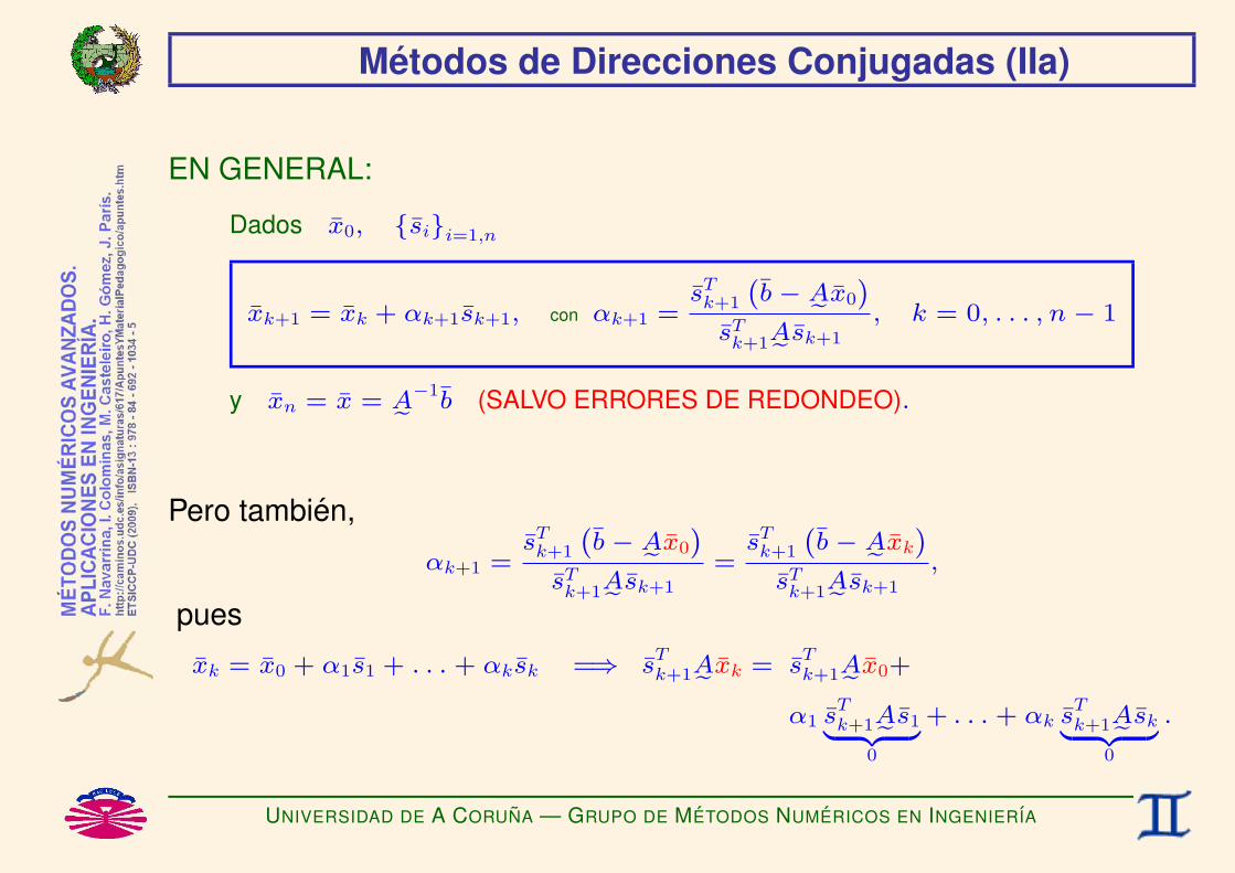
EN GENERAL:
Dados x0, sii=1,n
xk+1 = xk + αk+1sk+1, con αk+1 =sT
k+1
`b− Ae x0
´sT
k+1Ae sk+1
, k = 0, . . . , n− 1
y xn = x = Ae−1b (SALVO ERRORES DE REDONDEO).
Pero tambien,
αk+1 =sT
k+1
`b− Ae x0
´sT
k+1Ae sk+1
=sT
k+1
`b− Ae xk
´sT
k+1Ae sk+1
,
pues
xk = x0 + α1s1 + . . . + αksk =⇒ sTk+1Ae xk = s
Tk+1Ae x0+
α1 sTk+1Ae s1| z
0
+ . . . + αk sTk+1Ae sk| z
0
.
UNIVERSIDAD DE A CORUNA — GRUPO DE METODOS NUMERICOS EN INGENIERIA

Metodos de Direcciones Conjugadas (IIb)
Y FINALMENTE:
Dados x0, sii=1,n
rk = b−A˜ xk, αk+1 =sT
k+1rk
sTk+1A˜ sk+1
,
xk+1 = xk + αk+1sk+1,
k = 0, . . . , n− 1,
y xn = x = A˜−1b (SALVO ERRORES DE REDONDEO).
PROBLEMA:
¿Como se genera la base de vectores conjugados sii=1,n?
UNIVERSIDAD DE A CORUNA — GRUPO DE METODOS NUMERICOS EN INGENIERIA

Metodos de Direcciones Conjugadas (IIIa)
OBTENCION DE UNA BASE DE VECTORES CONJUGADOS sii=1,n
I METODO DE GRAM-SCHMIT
I METODO DE GRADIENTES CONJUGADOS(caso particular de Gram-Schmit)
UNIVERSIDAD DE A CORUNA — GRUPO DE METODOS NUMERICOS EN INGENIERIA
Metodos de Direcciones Conjugadas (IIIb)
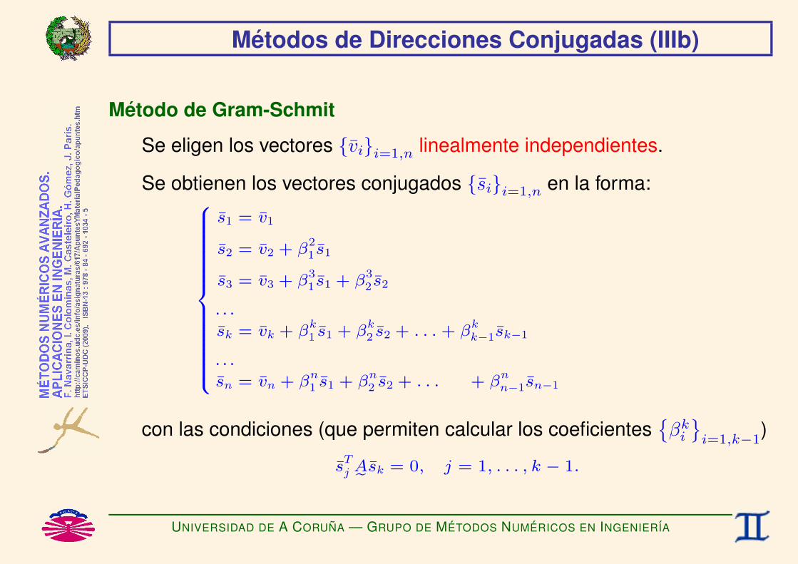
Metodo de Gram-Schmit
Se eligen los vectores vii=1,n linealmente independientes.
Se obtienen los vectores conjugados sii=1,n en la forma:
s1 = v1
s2 = v2 + β21s1
s3 = v3 + β31s1 + β
32s2
. . .sk = vk + β
k1 s1 + β
k2 s2 + . . .+ β
kk−1sk−1
. . .sn = vn + β
n1 s1 + β
n2 s2 + . . . + β
nn−1sn−1
con las condiciones (que permiten calcular los coeficientesβkii=1,k−1
)
sTj A˜ sk = 0, j = 1, . . . , k − 1.
UNIVERSIDAD DE A CORUNA — GRUPO DE METODOS NUMERICOS EN INGENIERIA

Metodos de Direcciones Conjugadas (IIIc)
Luego
sk = vk +
k−1Xi=1
βki si
sTj Ae sk = 0,
9>>>=>>>; =⇒ sTj Ae
vk +
k−1Xi=1
βki si
!= 0, j = 1, . . . , k−1,
y por consiguiente
sTj Ae vk +
βkj
“sTj Ae sj
”z | k−1Xi=1
βki
“s
Tj Ae si
”= 0 =⇒ β
kj = −
sTj Ae vk
sTj Ae sj
j = 1, . . . , k − 1.
UNIVERSIDAD DE A CORUNA — GRUPO DE METODOS NUMERICOS EN INGENIERIA

Metodos de Direcciones Conjugadas (IIId)
Y FINALMENTE:
Dados vii=1,n
s1 = v1,
βkj = −
sTj A˜ vk
sTj A˜ sj
, j = 1, . . . , k − 1,
sk = vk +k−1∑i=1
βki si,
k = 2, . . . , n.
PROBLEMA: Gran coste computacional, T (n3).
UNIVERSIDAD DE A CORUNA — GRUPO DE METODOS NUMERICOS EN INGENIERIA

Metodos de Direcciones Conjugadas (IV)
PREGUNTA:
¿Es posible elegir (habilmente) los vectores vii=1,n de forma que lamayor parte de los coeficientes
βk
i
i=1,k−1; k=2,n
sean nulos?
Respuesta:
SI: Metodo de Gradientes Conjugados
UNIVERSIDAD DE A CORUNA — GRUPO DE METODOS NUMERICOS EN INGENIERIA

Metodo de Gradientes Conjugados [CG] (Ia)
Dado el sistema
Ae x = b,
definimos la funcion cuadratica
f(x) =1
2x
TAe x− b
Tx + c,
cuyo gradiente es
∇f =
„df
dx
«T
= Ae x− b.
Luego,
∇f(xi) = −ri, siendo ri = b− Ae xi el residuo en la aproximacion xi.
UNIVERSIDAD DE A CORUNA — GRUPO DE METODOS NUMERICOS EN INGENIERIA

Metodo de Gradientes Conjugados [CG] (Ib)
Si elegimos como vectores vii=1,n los gradientes (cambiados de signo)8>>>>>>>>>>>>><>>>>>>>>>>>>>:
v1 = −∇f(x0) = r0 =`b− Ae x0
´v2 = −∇f(x1) = r1 =
`b− Ae x1
´v3 = −∇f(x2) = r2 =
`b− Ae x2
´. . .vk = −∇f(xk−1) = rk−1 =
`b− Ae xk−1
´. . .vn = −∇f(xn−1) = rn−1 =
`b− Ae xn−1
´entonces sucede que (*)
βkj = −
sTj Ae rk−1
sTj Ae sj
(= 0, j = 1, . . . , k − 2
6= 0, j = k − 1
(*) Se comprueba que esto es ası aunque no es evidente (ver equivalencias).
UNIVERSIDAD DE A CORUNA — GRUPO DE METODOS NUMERICOS EN INGENIERIA

Metodo de Gradientes Conjugados [CG] (Ic)
FINALMENTE, LA BASE DE GRADIENTES CONJUGADOS ES (*):
r0 = b−A˜ x0
s1 = r0,
rk−1 = b−A˜ xk−1
βkk−1 = −
sTk−1A˜ rk−1
sTk−1A˜ sk−1
,
sk = rk−1 + βkk−1sk−1,
k = 2, . . . , n.
(*) EN LO SUCESIVO PRESCINDIREMOS DEL SUPERINDICE k EN βkk−1
(ya que no es necesario).
UNIVERSIDAD DE A CORUNA — GRUPO DE METODOS NUMERICOS EN INGENIERIA
Metodo de Gradientes Conjugados [CG] (IIa)
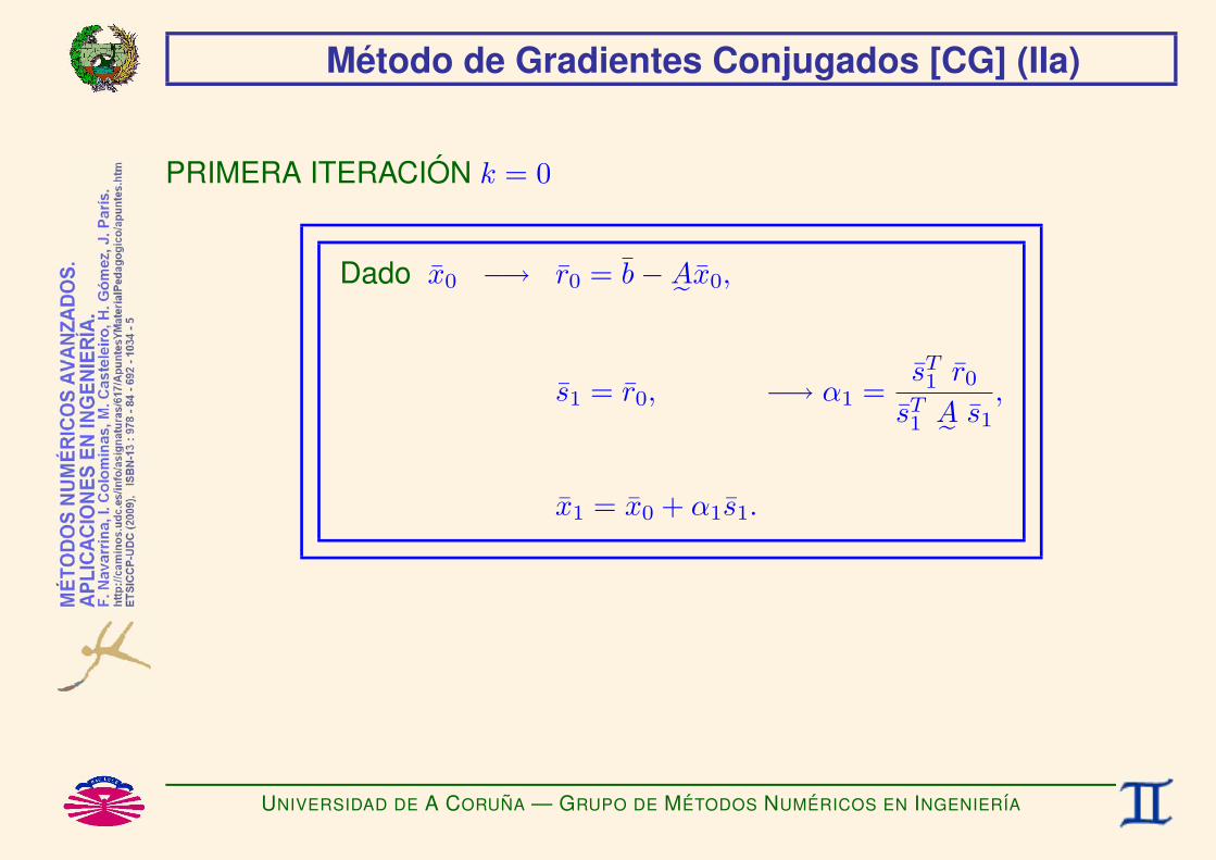
PRIMERA ITERACION k = 0
Dado x0 −→ r0 = b−A˜ x0,
s1 = r0, −→ α1 =sT1 r0
sT1 A˜ s1
,
x1 = x0 + α1s1.
UNIVERSIDAD DE A CORUNA — GRUPO DE METODOS NUMERICOS EN INGENIERIA

Metodo de Gradientes Conjugados [CG] (IIb)
ITERACIONES SIGUIENTES k = 1, . . . , n− 1
Dado xk −→ rk = b−A˜ xk, −→ βk = −sTk A˜ rk
sTk A˜ sk
,
sk+1 = rk + βksk, −→ αk+1 =sT
k+1 rk
sTk+1 A˜ sk+1
,
xk+1 = xk + αk+1sk+1,
Y xn verifica A˜ xn = b (SALVO ERRORES DE REDONDEO).
UNIVERSIDAD DE A CORUNA — GRUPO DE METODOS NUMERICOS EN INGENIERIA

Metodo de Gradientes Conjugados [CG] (IIc)
El algoritmo se detendra al finalizar el paso k. . .
I si k = n− 1, pues xk+1 = xn y por tanto verifica
rk+1 = b−A˜ xk+1 = 0 (salvo errores de redondeo *),
I o si ha convergido segun un criterio tipo‖xk+1 − xk‖ ≤maxεx, rx ‖xk‖ y
‖rk+1‖ ≤maxεr, rr
∥∥b∥∥
(*) Se suelen realizar algunas iteraciones mas para refinar la solucion.
UNIVERSIDAD DE A CORUNA — GRUPO DE METODOS NUMERICOS EN INGENIERIA

Metodo de Gradientes Conjugados [CG] (IIIa)
Equivalencias
1) sTk+1A˜ sk+1 = sTk+1A˜ rk,pues sk+1 = rk + βksk,
y sTk+1A˜ sk = 0.
2) rk+1 = rk − αk+1A˜ sk+1,pues rk+1 = b− A˜ xk+1 = b− A˜
(xk + αk+1sk+1
)=(b− A˜ xk)− αk+1A˜ sk+1 = rk − αk+1A˜ sk+1.
3) sTk+1rk+1 = 0, LUEGO EL AVANCE ES OPTIMO (*),
pues sTk+1rk+1 = s
Tk+1
(rk − αk+1A˜ sk+1
)= s
Tk+1rk − αk+1
(sTk+1A˜ sk+1
)
y αk+1 =sTk+1rk
sTk+1
A˜ sk+1
.
(*) Vease el planteamiento de mınima energıa.
UNIVERSIDAD DE A CORUNA — GRUPO DE METODOS NUMERICOS EN INGENIERIA

Metodo de Gradientes Conjugados [CG] (IIIb)
4) A˜ sk = − 1αk
(rk − rk−1),pues rk = rk−1 − αkAe sk (por la equivalencia 2).
5) (rk − rk−1)T
sk = (rk − rk−1)T
rk−1,pues s
Tk Ae sk = s
Tk Ae rk−1 (por la equivalencia 1) =⇒ s
Tk`Ae sk
´= r
Tk−1
`Ae sk
´,
luego sTk
−
1
αk
“rk − rk−1
”!= r
Tk−1
−
1
αk
“rk − rk−1
”!(por la equivalencia 4).
6) sTk+1rk = rT
k rk,
pues sk+1 = rk + βksk =⇒ sTk+1rk = r
Tk rk + βks
Tk rk,
y sTk rk = 0 (por la equivalencia 3).
UNIVERSIDAD DE A CORUNA — GRUPO DE METODOS NUMERICOS EN INGENIERIA

Metodo de Gradientes Conjugados [CG] (IIIc)
7) rTk+1rk = 0,
pues rTk+1rk =
“rk − αk+1Ae sk+1
”Trk (por la equivalencia 2)
= rTk rk − αk+1
“sTk+1Ae rk
”= r
Tk rk − αk+1
“sTk+1Ae sk+1
”(por la equivalencia 1)
y αk+1 =sTk+1rk
sTk+1
Ae sk+1
=rTk rk
sTk+1
Ae sk+1
(por la equivalencia 6).
UNIVERSIDAD DE A CORUNA — GRUPO DE METODOS NUMERICOS EN INGENIERIA
Metodo de Gradientes Conjugados [CG] (IIId)
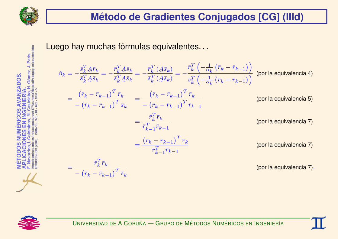
Luego hay muchas formulas equivalentes. . .
βk = −sTk Ae rk
sTk
Ae sk
= −rTk Ae sk
sTk
Ae sk
= −rTk (Ae sk)
sTk
(Ae sk)= −
rTk
“− 1
αk
`rk − rk−1
´”sTk
“− 1
αk
`rk − rk−1
´” (por la equivalencia 4)
=
`rk − rk−1
´Trk
−`rk − rk−1
´Tsk
=
`rk − rk−1
´Trk
−`rk − rk−1
´Trk−1
(por la equivalencia 5)
=rTk rk
rTk−1
rk−1
(por la equivalencia 7)
=
`rk − rk−1
´Trk
rTk−1
rk−1
(por la equivalencia 7)
=rTk rk
−`rk − rk−1
´Tsk
(por la equivalencia 7).
UNIVERSIDAD DE A CORUNA — GRUPO DE METODOS NUMERICOS EN INGENIERIA

Metodo de Gradientes Conjugados [CG] (IV)
Formulas equivalentes para el calculo del coeficiente βk
βk = −sTk A˜ rk
sTk A˜ sk
βk =[rk − rk−1]T rk
−[rk − rk−1]T skHESTENES–STIEFEL
βk =rTk rk
rTk−1 rk−1
FLETCHER–REEVES
βk =[rk − rk−1]T rk
rTk−1 rk−1
POLAK–RIBIERE
βk =rTk rk
−[rk − rk−1]T skMYERS
UNIVERSIDAD DE A CORUNA — GRUPO DE METODOS NUMERICOS EN INGENIERIA

Planteamiento de Mınima Energıa (I)
Sea el problema:
Hallar x,
que VERIFICA r = 0,
siendo r = b−A˜ x,
con
A˜ = A˜T (A˜ SIMETRICA),
vTA˜ v > 0 ∀v 6= 0 (A˜ DEF. +).
El problema anterior tambien puede escribirse en la forma siguiente...
UNIVERSIDAD DE A CORUNA — GRUPO DE METODOS NUMERICOS EN INGENIERIA

Planteamiento de Mınima Energıa (II)
MINIMA ENERGIA
Hallar x,
que MINIMIZA f(x) =12
xTA˜ x− xT b, (∗)
con
A˜ = A˜T (A˜ SIMETRICA),
vTA˜ v > 0 ∀v 6= 0 (A˜ DEF. +).
(*) Pues ∇f(x) =h
dfdx
iT
= −r, siendo r = b− Ae x.
UNIVERSIDAD DE A CORUNA — GRUPO DE METODOS NUMERICOS EN INGENIERIA

Planteamiento de Mınima Energıa (IIIa)
AVANCE OPTIMO
Si aplicamos al problema anterior un metodo numerico tipo
xk+1 = xk + αk+1sk+1
diremos que el avance αk+1 es optimo cuando se cumpla
αk+1 = minα
Φ(α), con Φ(α) = f(x)
∣∣∣∣∣x=xk+αsk+1
,
o lo que es lo mismo . . .
UNIVERSIDAD DE A CORUNA — GRUPO DE METODOS NUMERICOS EN INGENIERIA

Planteamiento de Mınima Energıa (IIIb)
dΦdα
∣∣∣α=αk+1
= 0, siendodΦdα
=df
dx
∣∣∣∣∣x=xk+αsk+1
sk+1
= −(b−A˜ (xk + αsk+1)
)Tsk+1.
Por tanto, la condicion de avance optimo es
rTk+1sk+1 = 0 ⇐⇒ sT
k+1rk+1 = 0,
que tambien puede escribirse como
αk+1 =sT
k+1rk
sTk+1A˜T sk+1
,
luego LOS METODOS DE DIRECCIONES CONJUGADAS SON DE AVANCE OPTIMO.
UNIVERSIDAD DE A CORUNA — GRUPO DE METODOS NUMERICOS EN INGENIERIA

Planteamiento de Mınima Energıa (IIIc)
AVANCE OPTIMO
UNIVERSIDAD DE A CORUNA — GRUPO DE METODOS NUMERICOS EN INGENIERIA

Precondicionamiento (I)
Sea el sistemaAe x = b.
Sea el precondicionador
Pe = EeEeT, con det(Ee) 6= 0.
Reescribimos el sistema original en la forma“Ee−1
AeEe−T”
| z bAe“
EeTx”
| z bx=“
Ee−1b”
| z bb,
y esperamos que al aplicar el Metodo de Gradientes Conjugados al sistemaprecondicionado bAebx = bbel proceso converja mas rapidamente a la solucion que en el caso delsistema original.
UNIVERSIDAD DE A CORUNA — GRUPO DE METODOS NUMERICOS EN INGENIERIA

Precondicionamiento (IIa)
PRIMERA ITERACION k = 0
Dado x0 = E˜T x0 −→ r0 = b− A˜ x0,
s1 = r0, −→ α1 =sT1 r0
sT1 A˜ s1
,
x1 = x0 + α1s1.
UNIVERSIDAD DE A CORUNA — GRUPO DE METODOS NUMERICOS EN INGENIERIA

Precondicionamiento (IIb)
ITERACIONES SIGUIENTES k > 0
Dado xk −→ rk = b− A˜ xk, −→ βk = −sTk A˜ rk
sTk A˜ sk
,
sk+1 = rk + βksk, −→ αk+1 =sT
k+1 rk
sTk+1 A˜ sk+1
,
xk+1 = xk + αk+1sk+1,
Y xn = E˜−T xn verifica A˜ xn = b (SALVO ERRORES DE REDONDEO).
UNIVERSIDAD DE A CORUNA — GRUPO DE METODOS NUMERICOS EN INGENIERIA

Precondicionamiento (IIIa)
Relacion del problema precondicionado con el problema original
1) bxk = EeTxk −→ brk = bb− bAeEeT
xk
= Ee−1b−
“Ee−1
AeEe−T”
EeTxk
= Ee−1b− Ee−1
Ae“
Ee−TEeT”
xk
= Ee−1b− Ee−1
Ae xk
= Ee−1 `b− Ae xk
´= Ee−1
rk, con rk = b− Ae xk.
UNIVERSIDAD DE A CORUNA — GRUPO DE METODOS NUMERICOS EN INGENIERIA

Precondicionamiento (IIIb)
2) bxk+1 = EeTxk+1 −→ xk+1 = Ee−T
(bxk + bαk+1bsk+1)
=“
Ee−TEeT”
xk + bαk+1Ee−Tbsk+1
= xk + bαk+1sk+1, con sk+1 = Ee−Tbsk+1.
sk+1 = Ee−T“brk + bβkbsk
”= Ee−T
“Ee−1
rk + bβkEeTsk
”=“
EeEeT”−1
rk + bβksk
= Pe−1rk + bβksk.
UNIVERSIDAD DE A CORUNA — GRUPO DE METODOS NUMERICOS EN INGENIERIA

Precondicionamiento (IIIc)
3)
bαk+1 =bsT
k+1brkbsTk+1bAebsk+1
=
`EeT sk+1
´T `Ee−1rk
´`EeT sk+1
´T `Ee−1AeEe−T
´ `EeT sk+1
´=
sTk+1
`EeEe−1
´rk
sTk+1
`EeEe−1
´Ae `E−Te EeT
´sk+1
=sT
k+1rk
sTk+1Ae sk+1
.
UNIVERSIDAD DE A CORUNA — GRUPO DE METODOS NUMERICOS EN INGENIERIA

Precondicionamiento (IIId)
4) bβk = −bsT
kbAebrkbsT
kbAebsk
= −`EeT sk
´T `Ee−1AeEe−T
´ `Ee−1rk
´`EeT sk
´T `Ee−1AeEe−T
´ `EeT sk
´= −
sTk
`EeEe−1
´Ae `E−Te Ee−1
´rk
sTk
`EeEe−1
´Ae `Ee−TEeT
´sk
= −sT
k Ae `EeEeT´−1
rk
sTk Ae sk
= −sT
k AePe−1rk
sTk Ae sk
.
UNIVERSIDAD DE A CORUNA — GRUPO DE METODOS NUMERICOS EN INGENIERIA
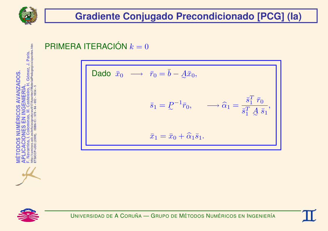
Gradiente Conjugado Precondicionado [PCG] (Ia)
PRIMERA ITERACION k = 0
Dado x0 −→ r0 = b−A˜ x0,
s1 = P˜−1r0, −→ α1 =sT1 r0
sT1 A˜ s1
,
x1 = x0 + α1s1.
UNIVERSIDAD DE A CORUNA — GRUPO DE METODOS NUMERICOS EN INGENIERIA

Gradiente Conjugado Precondicionado [PCG] (Ib)
ITERACIONES SIGUIENTES k > 0
Dado xk −→ rk = b−A˜ xk, −→ βk = −sTk A˜ P˜−1 rk
sTk A˜ sk
,
sk+1 = P˜−1rk + βksk, −→ αk+1 =sT
k+1 rk
sTk+1 A˜ sk+1
,
xk+1 = xk + αk+1sk+1,
Y xn verifica A˜ xn = b (SALVO ERRORES DE REDONDEO).
UNIVERSIDAD DE A CORUNA — GRUPO DE METODOS NUMERICOS EN INGENIERIA

Gradiente Conjugado Precondicionado [PCG] (Ic)
El algoritmo se detendra al finalizar el paso k. . .
I si k = n− 1, pues xk+1 = xn y por tanto verifica
rk+1 = b−A˜ xk+1 = 0 (salvo errores de redondeo *),
I o si ha convergido segun un criterio tipo‖xk+1 − xk‖ ≤maxεx, rx ‖xk‖ y
‖rk+1‖ ≤maxεr, rr
∥∥b∥∥
(*) Se suelen realizar algunas iteraciones mas para refinar la solucion.
UNIVERSIDAD DE A CORUNA — GRUPO DE METODOS NUMERICOS EN INGENIERIA

Gradiente Conjugado Precondicionado [PCG] (II)
Observaciones:
• Los sk son Ae–conjugados, pues
sTi Ae sj =
“Ee−Tbsi
”T “Ee bAeEeT
”“Ee−Tbsj
”= bsT
i
“Ee−1
Ee” bAe
“EeT
Ee−T” bsj
= bsTibAebsj.
• El avance es optimo, pues
sTk+1rk+1 =
“Ee−Tbsk+1
”T
(Eebrk+1) = bsTk+1
“Ee−1
Ee” brk+1
= bsTk+1brk+1.
• En generalr
Tk+1rk = (Eebrk+1)
T(Eebrk) = brT
k+1
“EeT
Ee” brk
6= 0.
UNIVERSIDAD DE A CORUNA — GRUPO DE METODOS NUMERICOS EN INGENIERIA

Gradiente Conjugado Precondicionado [PCG] (III)
CONCLUSIONES:
♥ Suele utilizarse el precondicionador diagonal P˜ = D˜ A.
♣ Para calcular xn el tiempo de computacion es T (n3).♣ NO ES MEJOR QUE LOS METODOS DIRECTOS (GAUSS, CHOLESKY), A MENOS QUE
CONVERJA ANTES.
♥ Es un metodo directo, pero funciona como los metodos iterativos ya que♥ PUEDE DETENERSE ANTICIPADAMENTE, LO QUE PROPORCIONA UN APROXIMACION A
LA SOLUCION.♦ NO MODIFICA LOS COEFICIENTES DE LA MATRIZ,♦ POR LO QUE PUEDE SER UTILIZADO CON ESQUEMAS DE ALMACENAMIENTO MINIMO
PARA MATRICES DISPERSAS.
♣ Puede ser muy ventajoso (o la unica alternativa posible) cuando lamatriz es no-estructurada y muy dispersa.
♦ EN TALES CASOS SUELE UTILIZARSE SIN ENSAMBLAR LA MATRIZ.
UNIVERSIDAD DE A CORUNA — GRUPO DE METODOS NUMERICOS EN INGENIERIA
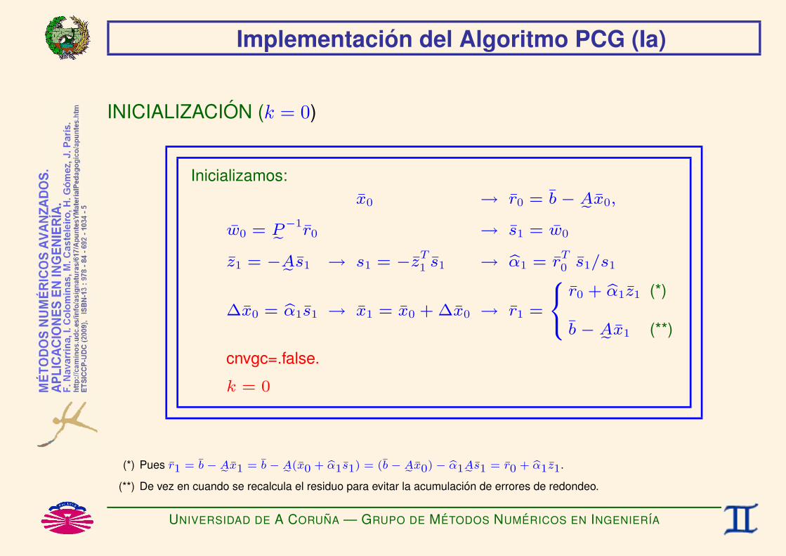
Implementacion del Algoritmo PCG (Ia)
INICIALIZACION (k = 0)
Inicializamos:x0 → r0 = b− Ae x0,
w0 = Pe−1r0 → s1 = w0
z1 = −Ae s1 → s1 = −zT1 s1 → bα1 = r
T0 s1/s1
∆x0 = bα1s1 → x1 = x0 + ∆x0 → r1 =
8<:r0 + bα1z1 (*)
b− Ae x1 (**)
cnvgc=.false.
k = 0
(*) Pues r1 = b− Ae x1 = b− Ae(x0 + bα1s1) = (b− Ae x0)− bα1Ae s1 = r0 + bα1z1.
(**) De vez en cuando se recalcula el residuo para evitar la acumulacion de errores de redondeo.
UNIVERSIDAD DE A CORUNA — GRUPO DE METODOS NUMERICOS EN INGENIERIA
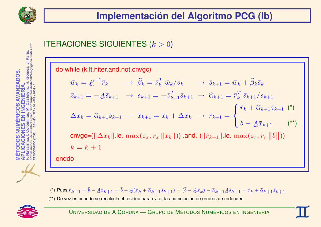
Implementacion del Algoritmo PCG (Ib)
ITERACIONES SIGUIENTES (k > 0)
do while (k.lt.niter.and.not.cnvgc)
wk = Pe−1rk → bβk = z
Tk wk/sk → sk+1 = wk + bβksk
zk+1 = −Ae sk+1 → sk+1 = −zTk+1sk+1 → bαk+1 = r
Tk sk+1/sk+1
∆xk = bαk+1sk+1 → xk+1 = xk + ∆xk → rk+1 =
8<:rk + bαk+1zk+1 (*)
b− Ae xk+1 (**)
cnvgc=(‖∆xk‖.le. max(εx, rx ‖xk‖)) .and. (‖rk+1‖.le. max(εr, rr
‚‚b‚‚))
k = k + 1
enddo
(*) Pues rk+1 = b− Ae xk+1 = b− Ae(xk + bαk+1sk+1) = (b− Ae xk)− bαk+1Ae sk+1 = rk + bαk+1zk+1.
(**) De vez en cuando se recalcula el residuo para evitar la acumulacion de errores de redondeo.
UNIVERSIDAD DE A CORUNA — GRUPO DE METODOS NUMERICOS EN INGENIERIA
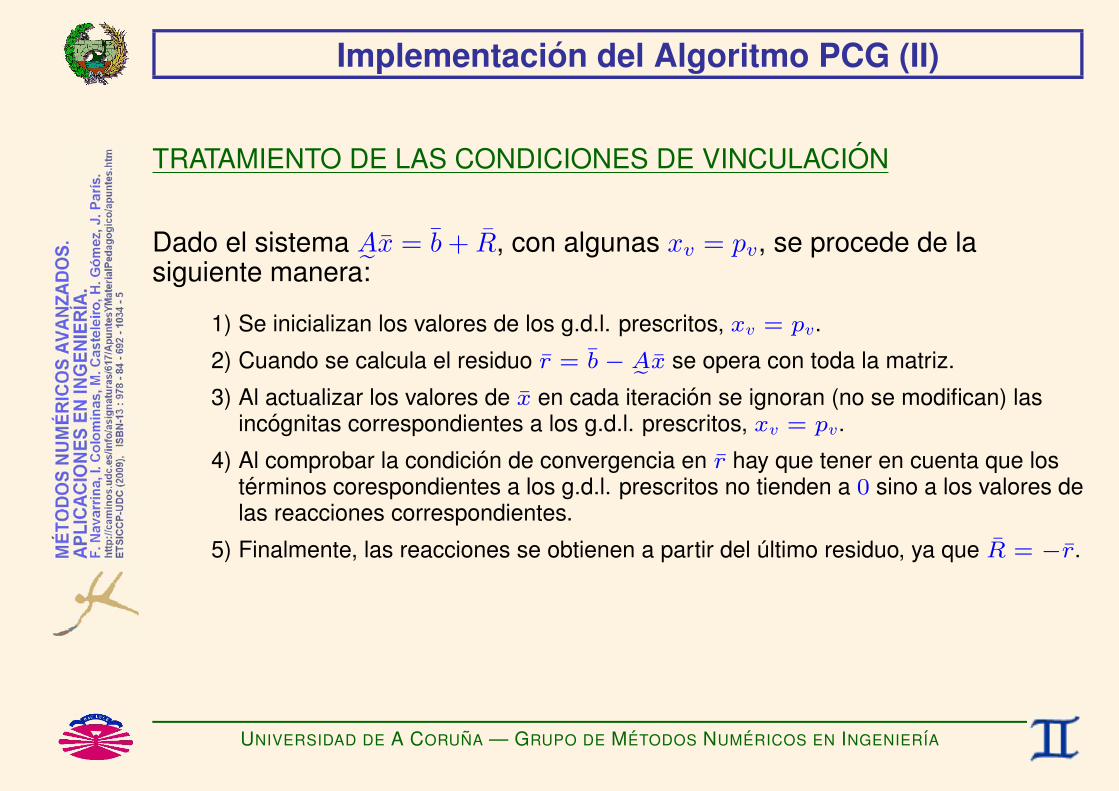
Implementacion del Algoritmo PCG (II)
TRATAMIENTO DE LAS CONDICIONES DE VINCULACION
Dado el sistema A˜ x = b + R, con algunas xv = pv, se procede de lasiguiente manera:
1) Se inicializan los valores de los g.d.l. prescritos, xv = pv.
2) Cuando se calcula el residuo r = b− Ae x se opera con toda la matriz.
3) Al actualizar los valores de x en cada iteracion se ignoran (no se modifican) lasincognitas correspondientes a los g.d.l. prescritos, xv = pv.
4) Al comprobar la condicion de convergencia en r hay que tener en cuenta que losterminos corespondientes a los g.d.l. prescritos no tienden a 0 sino a los valores delas reacciones correspondientes.
5) Finalmente, las reacciones se obtienen a partir del ultimo residuo, ya que R = −r.
UNIVERSIDAD DE A CORUNA — GRUPO DE METODOS NUMERICOS EN INGENIERIA


METODOS SEMI-ITERATIVOS PARAGRANDES SISTEMAS DE ECUACIONES LINEALES:
GENERALIZACIONF. Navarrina, I. Colominas, M. Casteleiro, H. Gomez, J. Parıs
GMNI — GRUPO DE METODOS NUMERICOS EN INGENIERIA
Departamento de Metodos Matematicos y de RepresentacionEscuela Tecnica Superior de Ingenieros de Caminos, Canales y Puertos
Universidad de A Coruna, Espana
e-mail: [email protected] web: http://caminos.udc.es/gmni
UNIVERSIDAD DE A CORUNA — GRUPO DE METODOS NUMERICOS EN INGENIERIA

INDICE
I Planteamientos Alternativos
I Residuos Ponderados
I Mınimos Cuadrados
I Principio Variacional
I Mınima Energıa
I Metodos de Krylov
I Matrices no simetricas
UNIVERSIDAD DE A CORUNA — GRUPO DE METODOS NUMERICOS EN INGENIERIA

Planteamientos Alternativos (I)
Sea el problema:
Hallar x,
que verifica A˜ x = b,
donde la matriz A˜ es no singular (pero no necesariamente simetrica nidefinida positiva).
El problema anterior puede escribirse en las formas alternativas...
UNIVERSIDAD DE A CORUNA — GRUPO DE METODOS NUMERICOS EN INGENIERIA

Planteamientos Alternativos (IIa)
a) FORMA ORIGINAL
Hallar x,
que VERIFICA r = 0,
siendo r = b−A˜ x.
UNIVERSIDAD DE A CORUNA — GRUPO DE METODOS NUMERICOS EN INGENIERIA

Planteamientos Alternativos (IIb)
b) RESIDUOS PONDERADOS
Hallar x,
que VERIFICA ωT r = 0 ∀ω,
siendo r = b−A˜ x.
UNIVERSIDAD DE A CORUNA — GRUPO DE METODOS NUMERICOS EN INGENIERIA

Planteamientos Alternativos (IIc1)
c) MINIMOS CUADRADOS (O MINIMO RESIDUO)
Hallar x,
que MINIMIZA g(x) = rTB˜ r, (*)
siendo r = b−A˜ x,
(*) Be SIMETRICA Y DEFINIDA POSITIVA.
UNIVERSIDAD DE A CORUNA — GRUPO DE METODOS NUMERICOS EN INGENIERIA

Planteamientos Alternativos (IIc2)
. . . que equivale a decir
Hallar x,
que VERIFICA ∇g(x) = 0,
siendo ∇g(x) =[dg
dx
]T
= −2A˜TB˜ r, (*)
r = b−A˜ x,
(*) Be SIMETRICA Y DEFINIDA POSITIVA.
UNIVERSIDAD DE A CORUNA — GRUPO DE METODOS NUMERICOS EN INGENIERIA
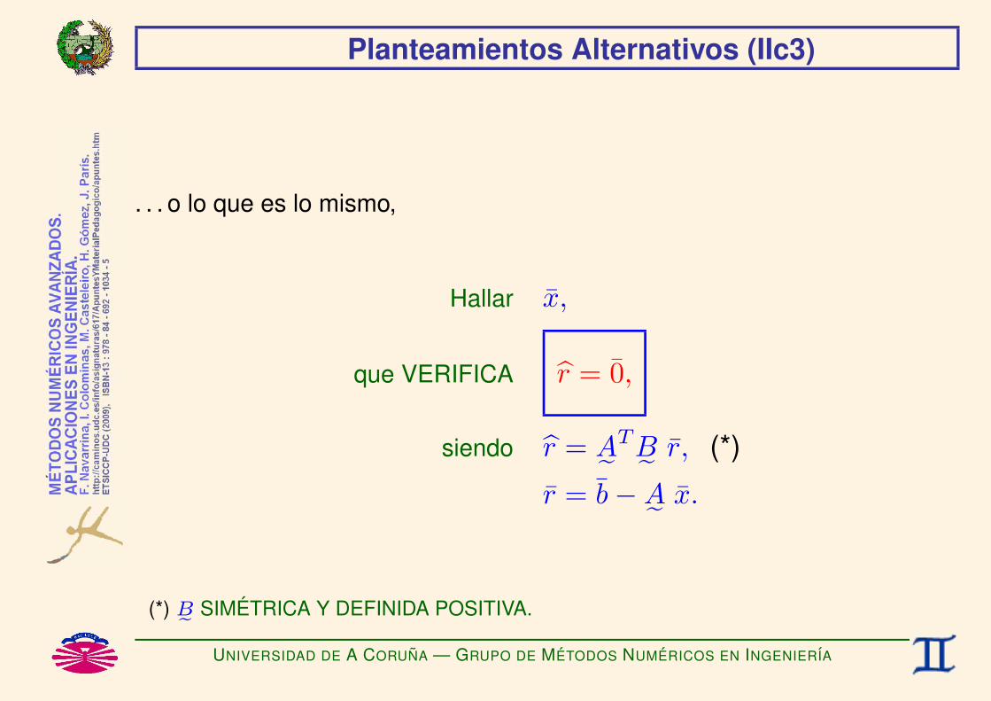
Planteamientos Alternativos (IIc3)
. . . o lo que es lo mismo,
Hallar x,
que VERIFICA r = 0,
siendo r = A˜TB˜ r, (*)
r = b−A˜ x.
(*) Be SIMETRICA Y DEFINIDA POSITIVA.
UNIVERSIDAD DE A CORUNA — GRUPO DE METODOS NUMERICOS EN INGENIERIA

Planteamientos Alternativos (IIc4)
I Luego,
♦ Transforma el sistema original Ae x = b en otro
Ax = b, siendo
bA=A˜T B˜ A˜, (SIMETRICA, DEF +)bb=A˜T B˜ b.
♥ A este sistema puede aplicarsele el metodo de gradientes conjugados.Basta con calcular el residuobr = AeT
“Be r”
, con r = b− Ae x. (*)
♣ Para aplicar el PCG hay que calcular la diagonal de la matriz bAe = AeTBe Ae . Si lamatriz A no se ha ensamblado (que es lo normal en estos casos), hay que obtenerlos coeficientesbajj = δ
TjbAe δj = δ
Tj AeT
Be Ae δj =`Ae δj
´TBe `Ae δj
´con δj = δiji=1,...,n
(*) El tiempo de calculo necesario para calcular el residuo se duplica (aproximadamente), ya que hay que ahora hay que realizardos productos matriciales importantes (uno con la matriz Ae y otro con su traspuesta). En general se elegira una matriz Bemuy vacıa para que el coste computacional de su producto matricial sea poco importante).
UNIVERSIDAD DE A CORUNA — GRUPO DE METODOS NUMERICOS EN INGENIERIA

Planteamientos Alternativos (IId1)
d) PRINCIPIO VARIACIONAL
Hallar x,
que VERIFICAdJ(λ)
dλ
∣∣∣∣λ=0
= 0 ∀δx,
siendo J(λ) =(b−A˜ (x + λδx)
)TC˜ (b−A˜ (x + λδx)
), (*)
y por tantodJ(λ)
dλ
∣∣∣∣λ=0
= −2 (A˜ δx)TC˜ r,
r = b−A˜ x,
(*) Ce SIMETRICA Y DEFINIDA POSITIVA.
UNIVERSIDAD DE A CORUNA — GRUPO DE METODOS NUMERICOS EN INGENIERIA

Planteamientos Alternativos (IId2)
. . . que equivale a decir
Hallar x,
que VERIFICA − 2δxT(A˜TC˜ r
)= 0 ∀δx, (*)
siendo r = b−A˜ x,
(*) Ce SIMETRICA Y DEFINIDA POSITIVA.
UNIVERSIDAD DE A CORUNA — GRUPO DE METODOS NUMERICOS EN INGENIERIA

Planteamientos Alternativos (IId3)
. . . o lo que es lo mismo
Hallar x,
que VERIFICA ωT r = 0 ∀ω = C˜A˜δx, (*)
siendo r = b−A˜ x,
(*) Ce SIMETRICA Y DEFINIDA POSITIVA.
UNIVERSIDAD DE A CORUNA — GRUPO DE METODOS NUMERICOS EN INGENIERIA

Planteamientos Alternativos (IId4)
. . . o lo que es lo mismo
Hallar x,
que VERIFICA r = 0,
siendo r = A˜TC˜ r, (*)
r = b−A˜ x.
(*) Ce SIMETRICA Y DEFINIDA POSITIVA.
UNIVERSIDAD DE A CORUNA — GRUPO DE METODOS NUMERICOS EN INGENIERIA
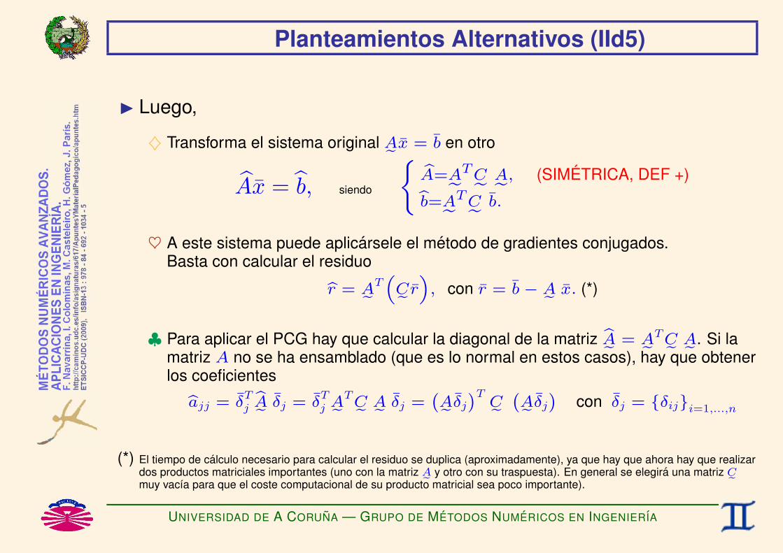
Planteamientos Alternativos (IId5)
I Luego,
♦ Transforma el sistema original Ae x = b en otro
Ax = b, siendo
bA=A˜T C˜ A˜, (SIMETRICA, DEF +)bb=A˜T C˜ b.
♥ A este sistema puede aplicarsele el metodo de gradientes conjugados.Basta con calcular el residuobr = AeT
“Ce r”
, con r = b− Ae x. (*)
♣ Para aplicar el PCG hay que calcular la diagonal de la matriz bAe = AeTCe Ae . Si lamatriz A no se ha ensamblado (que es lo normal en estos casos), hay que obtenerlos coeficientesbajj = δ
TjbAe δj = δ
Tj AeT
Ce Ae δj =`Ae δj
´TCe `Ae δj
´con δj = δiji=1,...,n
(*) El tiempo de calculo necesario para calcular el residuo se duplica (aproximadamente), ya que hay que ahora hay que realizardos productos matriciales importantes (uno con la matriz Ae y otro con su traspuesta). En general se elegira una matriz Cemuy vacıa para que el coste computacional de su producto matricial sea poco importante).
UNIVERSIDAD DE A CORUNA — GRUPO DE METODOS NUMERICOS EN INGENIERIA

Planteamientos Alternativos (IIe)
e) MINIMA ENERGIA (A˜ SIMETRICA Y DEFINIDA POSITIVA)
Hallar x,
que MINIMIZA f(x) =12
xTA˜ x− xT b, (*)
con
A˜ = A˜T (A˜ SIMETRICA),
vTA˜ v > 0 ∀v 6= 0 (A˜ DEF. +).
(*) Pues ∇f(x) =h
dfdx
iT
= −r, siendo r = b− Ae x.
UNIVERSIDAD DE A CORUNA — GRUPO DE METODOS NUMERICOS EN INGENIERIA

Residuos Ponderados (I)
PLANTEAMIENTO EN RESIDUOS PONDERADOS
r = b−A˜ x = 0 ⇐⇒ ωT r = 0 ∀ω.
UNIVERSIDAD DE A CORUNA — GRUPO DE METODOS NUMERICOS EN INGENIERIA
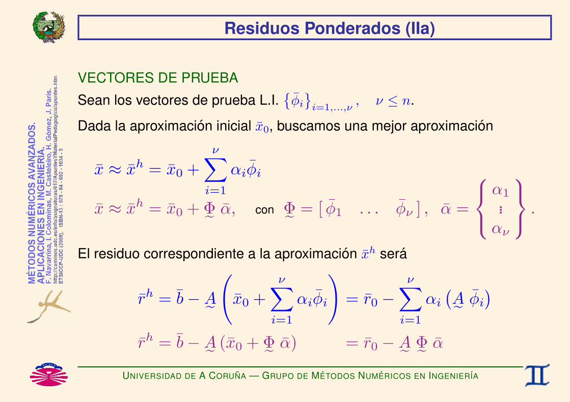
Residuos Ponderados (IIa)
VECTORES DE PRUEBA
Sean los vectores de prueba L.I.φi
i=1,...,ν
, ν ≤ n.
Dada la aproximacion inicial x0, buscamos una mejor aproximacion
x ≈ xh = x0 +ν∑
i=1
αiφi
x ≈ xh = x0 + Φ˜ α, con Φ˜ = [ φ1 . . . φν ] , α =
α1...
αν
.
El residuo correspondiente a la aproximacion xh sera
rh = b−A˜(
x0 +ν∑
i=1
αiφi
)= r0 −
ν∑i=1
αi
(A˜ φi
)rh = b−A˜ (x0 + Φ˜ α) = r0 −A˜ Φ˜ α
UNIVERSIDAD DE A CORUNA — GRUPO DE METODOS NUMERICOS EN INGENIERIA

Residuos Ponderados (IIb)
En general no sera posible que xh = x (*), por lo que
rh 6= 0 ⇐⇒ no es posible que ωT rh = 0 ∀ω.
(*) Salvo que x− x0 este contenido en el subespacio generado por los vectores de prueba.
UNIVERSIDAD DE A CORUNA — GRUPO DE METODOS NUMERICOS EN INGENIERIA

Residuos Ponderados (IIIa)
VECTORES DE TEST
Sean los vectores de test L.I. ωjj=1,...,ν , ν ≤ n.
Sea
ωh =ν∑
j=1
βjωj
ωh = Ω˜ β, con Ω˜ = [ ω1 . . . ων ] , β =
β1...
βν
.
Nos proponemos obtener la aproximacion xh que verifique
(ωh)T
rh = 0 ∀ωh.
UNIVERSIDAD DE A CORUNA — GRUPO DE METODOS NUMERICOS EN INGENIERIA
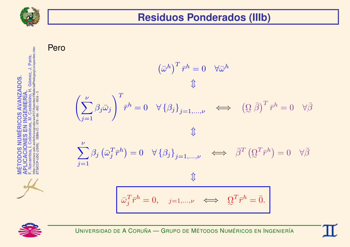
Residuos Ponderados (IIIb)
Pero (ωh)T
rh = 0 ∀ωh
m(ν∑
j=1
βjωj
)T
rh = 0 ∀ βjj=1,...,ν ⇐⇒(Ω˜ β
)Trh = 0 ∀β
mν∑
j=1
βj
(ωT
j rh)
= 0 ∀ βjj=1,...,ν ⇐⇒ βT(Ω˜T rh
)= 0 ∀β
m
ωTj rh = 0, j=1,...,ν ⇐⇒ Ω˜T rh = 0.
UNIVERSIDAD DE A CORUNA — GRUPO DE METODOS NUMERICOS EN INGENIERIA

Residuos Ponderados (IVa)
Por tanto,
ωTj
(r0 −
ν∑i=1
αi
(A˜ φi
))= 0, j=1,...,ν ⇐⇒ Ω˜T (r0 −A˜ Φ˜ α) = 0
m
ν∑i=1
kji︷ ︸︸ ︷(ωT
j A˜ φi
)αi =
fj︷ ︸︸ ︷ωT
j r0, j=1,...,ν ⇐⇒K˜︷ ︸︸ ︷(
Ω˜TA˜ Φ˜) α =
f︷ ︸︸ ︷Ω˜T r0
m
ν∑i=1
kjiαi = fj, j=1,...,ν ⇐⇒ K˜ α = f .
UNIVERSIDAD DE A CORUNA — GRUPO DE METODOS NUMERICOS EN INGENIERIA

Residuos Ponderados (IVb)
Luego el sistema original A˜ x = b (de orden n) ha sido sustituido por elsistema (de orden ν ≤ n)
K˜ α = f , con α = αii=1,...,νy
K˜ = [kji]i=1,...,νj=1,...,ν
, kji = ωTj A˜ φi ⇐⇒ K˜ = Ω˜TA˜ Φ˜
f = fjj=1,...,ν, fj = ωT
j r0 ⇐⇒ f = Ω˜T r0.
Posteriormente obtendremos la aproximacion a la solucion
xh = x0 +ν∑
i=1
αiφi ⇐⇒ xh = x0 + Φ˜ α.
UNIVERSIDAD DE A CORUNA — GRUPO DE METODOS NUMERICOS EN INGENIERIA
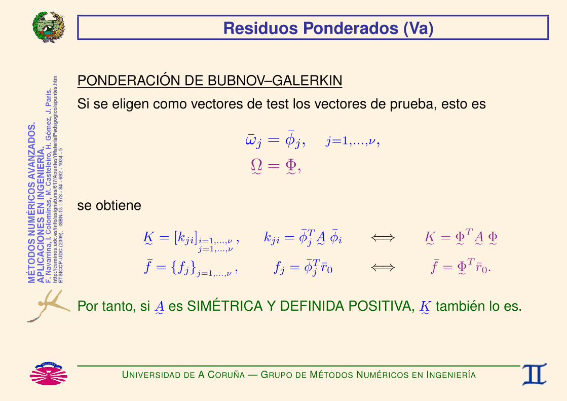
Residuos Ponderados (Va)
PONDERACION DE BUBNOV–GALERKIN
Si se eligen como vectores de test los vectores de prueba, esto es
ωj = φj, j=1,...,ν,
Ω˜ = Φ˜,
se obtiene
K˜ = [kji]i=1,...,νj=1,...,ν
, kji = φTj A˜ φi ⇐⇒ K˜ = Φ˜TA˜ Φ˜
f = fjj=1,...,ν, fj = φT
j r0 ⇐⇒ f = Φ˜T r0.
Por tanto, si A˜ es SIMETRICA Y DEFINIDA POSITIVA, K˜ tambien lo es.
UNIVERSIDAD DE A CORUNA — GRUPO DE METODOS NUMERICOS EN INGENIERIA

Residuos Ponderados (Vb)
Observamos que el metodo de GRADIENTES CONJUGADOS . . .
♣ es un metodo de RESIDUOS PONDERADOS
♣ con ponderacion del tipo BUBNOV-GALERKIN
♣ en el que los vectores de prueba (φi = si) son conjugados respecto a lamatriz A˜ ,
♥ por lo que la matriz K˜ es diagonal
♦ y los coeficientes α pueden obtenerse de forma explıcita mediante laexpresion
αj =sT
j r0
sTj A˜ sj
.
UNIVERSIDAD DE A CORUNA — GRUPO DE METODOS NUMERICOS EN INGENIERIA

Residuos Ponderados (VIa)
METODOS DE PROYECCION
Los METODOS DE RESIDUOS PONDERADOS tambien se denominan ası,
ya que siendo
x la solucion exacta, con r = b−A˜ x
xh la solucion aproximada, con rh = b−A˜ xh
se verifica(ωh)T
r = 0 ∀ωh
(ωh)T
rh = 0 ∀ωh
=⇒(ωh)T (
r − rh)
= 0 ∀ωh
=⇒−(ωh)T
A˜ (x− xh)
= 0 ∀ωh
=⇒−(A˜T ωh
)T (x− xh
)= 0 ∀ωh.
UNIVERSIDAD DE A CORUNA — GRUPO DE METODOS NUMERICOS EN INGENIERIA

Residuos Ponderados (VIb)
Luego, la solucion aproximada xh es
la PROYECCION de la solucion exacta x
sobre el subespacio formado por los vectores de prueba xh
segun la normal al subespacio formado por los vectores A˜T ωh.
UNIVERSIDAD DE A CORUNA — GRUPO DE METODOS NUMERICOS EN INGENIERIA

Mınimos Cuadrados (I)
PLANTEAMIENTO EN MINIMOS CUADRADOS
r = b−A˜ x = 0 ⇐⇒ Minimizar g(x) = rTB˜ r. (*)
(*) Be SIMETRICA Y DEFINIDA POSITIVA.
UNIVERSIDAD DE A CORUNA — GRUPO DE METODOS NUMERICOS EN INGENIERIA

Mınimos Cuadrados (II)
VECTORES DE PRUEBA
Sean los vectores de prueba L.I.φi
i=1,...,ν
, ν ≤ n.
Dada la aproximacion inicial x0, buscamos una mejor aproximacion
x ≈ xh = x0 +ν∑
i=1
αiφi
x ≈ xh = x0 + Φ˜ α, con Φ˜ = [ φ1 . . . φν ] , α =
α1...
αν
.
El residuo correspondiente a la aproximacion xh sera
rh = b−A˜(
x0 +ν∑
i=1
αiφi
)= r0 −
ν∑i=1
αi
(A˜ φi
)rh = b−A˜ (x0 + Φ˜ α) = r0 −A˜ Φ˜ α
UNIVERSIDAD DE A CORUNA — GRUPO DE METODOS NUMERICOS EN INGENIERIA

Mınimos Cuadrados (IIIa)
Sea
γ(α) = g(x)∣∣∣x=xh
=(rh)T
B˜ rh.
Nos proponemos obtener la aproximacion xh que verifique
∂γ
∂αj= 0, j=1,...,ν ⇐⇒
[dγ
dα
]T
= 0.
UNIVERSIDAD DE A CORUNA — GRUPO DE METODOS NUMERICOS EN INGENIERIA

Mınimos Cuadrados (IIIb)
Pero
∂γ
∂αj
=∂γ
∂rh
∂rh
∂αj
=
„2“
rh”T
Be« `−Ae φj
´= −2φ
Tj AeT
Be rh, j=1,...,ν
y
»∂γ
∂α
–T
=
∂γ
∂rh
∂rh
∂α
!T
=
„„2“
rh”T
Be«
(−AeΦe)
«T
= −2ΦeTAeT
Be rh,
luego,
∂γ∂αj
= 0, j=1,...,ν ⇐⇒[
dγdα
]T= 0
m
φTj A˜TB˜ rh = 0, j=1,...,ν ⇐⇒ Φ˜TA˜TB˜ rh = 0.
UNIVERSIDAD DE A CORUNA — GRUPO DE METODOS NUMERICOS EN INGENIERIA

Mınimos Cuadrados (IVa)
Por tanto,
φTj AeTBe
r0 −
νXi=1
αi
`Ae φi
´!= 0, j=1,...,ν ⇐⇒ ΦeTAeTBe (r0 − Ae Φe α) = 0
m
νXi=1
kjiz | “φ
Tj AeT
Be Ae φi
”αi =
fjz | φ
Tj AeT
Be r0, j=1,...,ν ⇐⇒
Kez | “ΦeT
AeTBe Ae Φe
”α =
fz | ΦeT
AeTBe r0
m
νXi=1
kjiαi = fj, j=1,...,ν ⇐⇒ Ke α = f .
UNIVERSIDAD DE A CORUNA — GRUPO DE METODOS NUMERICOS EN INGENIERIA
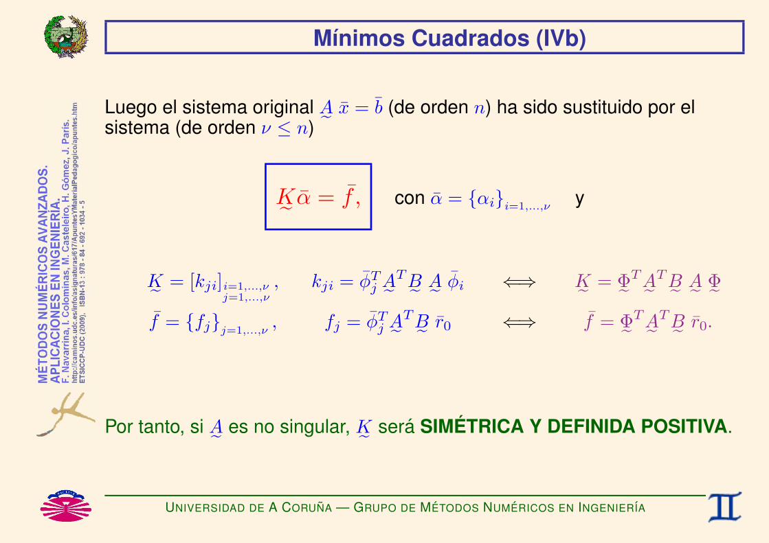
Mınimos Cuadrados (IVb)
Luego el sistema original A˜ x = b (de orden n) ha sido sustituido por elsistema (de orden ν ≤ n)
K˜ α = f , con α = αii=1,...,νy
K˜ = [kji]i=1,...,νj=1,...,ν
, kji = φTj A˜TB˜ A˜ φi ⇐⇒ K˜ = Φ˜TA˜TB˜ A˜ Φ˜
f = fjj=1,...,ν, fj = φT
j A˜TB˜ r0 ⇐⇒ f = Φ˜TA˜TB˜ r0.
Por tanto, si A˜ es no singular, K˜ sera SIMETRICA Y DEFINIDA POSITIVA.
UNIVERSIDAD DE A CORUNA — GRUPO DE METODOS NUMERICOS EN INGENIERIA
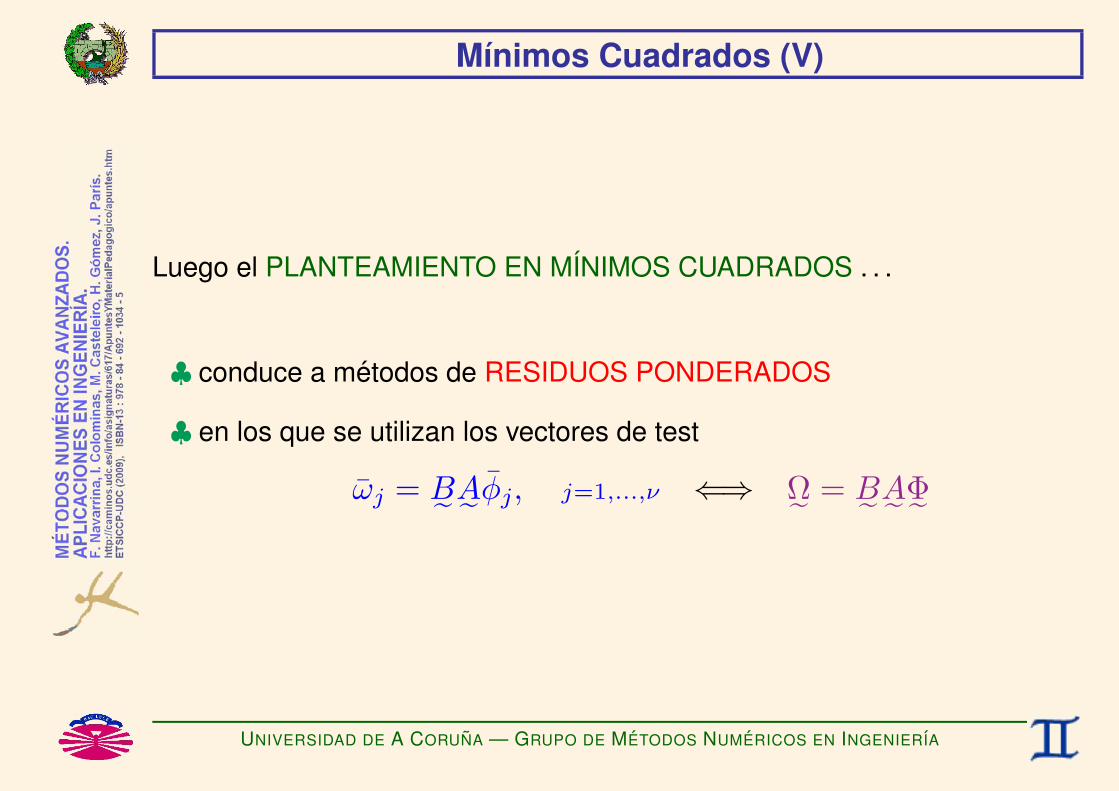
Mınimos Cuadrados (V)
Luego el PLANTEAMIENTO EN MINIMOS CUADRADOS . . .
♣ conduce a metodos de RESIDUOS PONDERADOS
♣ en los que se utilizan los vectores de test
ωj = B˜A˜ φj, j=1,...,ν ⇐⇒ Ω˜ = B˜A˜Φ˜
UNIVERSIDAD DE A CORUNA — GRUPO DE METODOS NUMERICOS EN INGENIERIA

Principio Variacional (I)
PLANTEAMIENTO VARIACIONAL
r = b−A˜ x = 0 ⇐⇒
dJ(λ)dλ
∣∣∣∣λ=0
∀δx, siendo
J(λ)=(b−A˜(x+λδx))TC˜(b−A˜(x+λδx)),
dJ(λ)dλ
∣∣∣∣λ=0
= −2 (A˜ δx)TC˜ r.
(*)
(*) Ce SIMETRICA Y DEFINIDA POSITIVA.
UNIVERSIDAD DE A CORUNA — GRUPO DE METODOS NUMERICOS EN INGENIERIA

Principio Variacional (II)
VECTORES DE PRUEBA
Sean los vectores de prueba L.I.φi
i=1,...,ν
, ν ≤ n.
Dada la aproximacion inicial x0, buscamos una mejor aproximacion
x ≈ xh = x0 +ν∑
i=1
αiφi
x ≈ xh = x0 + Φ˜ α, con Φ˜ = [ φ1 . . . φν ] , α =
α1...αν
.
El residuo correspondiente a la aproximacion xh sera
rh = b−A˜(
x0 +ν∑
i=1
αiφi
)= r0 −
ν∑i=1
αi
(A˜ φi
)rh = b−A˜ (x0 + Φ˜ α) = r0 −A˜ Φ˜ α
UNIVERSIDAD DE A CORUNA — GRUPO DE METODOS NUMERICOS EN INGENIERIA

Principio Variacional (IIIa)
PERTURBACION
Sea la perturbacion
δxh =ν∑
j=1
δαjφj
δxh = Φ˜ δα, con Φ˜ = [ φ1 . . . φν ] , δα =
δα1...
δαν
.
Nos proponemos obtener la aproximacion xh que verifique
−2(A˜ δxh
)TC˜ rh = 0 ∀δxh.
UNIVERSIDAD DE A CORUNA — GRUPO DE METODOS NUMERICOS EN INGENIERIA

Principio Variacional (IIIb)
Pero
`δxh´T
AeTCe rh = 0 ∀δxh
m0@ νXj=1
δαjφj
1AT
AeTCe r
h= 0 ∀ δαjj=1,...,ν ⇐⇒ (Φe δα)
TAeT
Ce rh
= 0 ∀δα
mνX
j=1
δαj
“φ
Tj AeT
Ce rh”
= 0 ∀ δαjj=1,...,ν ⇐⇒ δαT“ΦeT
AeTCe r
h”
= 0 ∀δα
m
φTj AeT
Ce rh
= 0, j=1,...,ν ⇐⇒ ΦeTAeT
Ce rh
= 0.
UNIVERSIDAD DE A CORUNA — GRUPO DE METODOS NUMERICOS EN INGENIERIA

Principio Variacional (IVa)
Por tanto,
φTj AeTCe
r0 −
νXi=1
αi
`Ae φi
´!= 0, j=1,...,ν ⇐⇒ ΦeTAeTCe (r0 − Ae Φe α) = 0
m
νXi=1
kjiz | “φ
Tj AeT
Ce Ae φi
”αi =
fjz | φ
Tj AeT
Ce r0, j=1,...,ν ⇐⇒
Kez | “ΦeT
AeTCe Ae Φe
”α =
fz | ΦeT
AeTCe r0
m
νXi=1
kjiαi = fj, j=1,...,ν ⇐⇒ Ke α = f .
UNIVERSIDAD DE A CORUNA — GRUPO DE METODOS NUMERICOS EN INGENIERIA

Principio Variacional (IVb)
Luego el sistema original A˜ x = b (de orden n) ha sido sustituido por elsistema (de orden ν ≤ n)
K˜ α = f , con α = αii=1,...,νy
K˜ = [kji]i=1,...,νj=1,...,ν
, kji = φTj A˜TC˜ A˜ φi ⇐⇒ K˜ = Φ˜TA˜TC˜ A˜ Φ˜
f = fjj=1,...,ν, fj = φT
j A˜TC˜ r0 ⇐⇒ f = Φ˜TA˜TC˜ r0.
Por tanto, si A˜ es no singular, K˜ sera SIMETRICA Y DEFINIDA POSITIVA.
UNIVERSIDAD DE A CORUNA — GRUPO DE METODOS NUMERICOS EN INGENIERIA

Principio Variacional (V)
Por tanto, el PLANTEAMIENTO VARIACIONAL . . .
♣ conduce a metodos de RESIDUOS PONDERADOS
♣ en los que se utilizan los vectores de test
ωj = C˜A˜ φj, j=1,...,ν ⇐⇒ Ω˜ = C˜A˜Φ˜
UNIVERSIDAD DE A CORUNA — GRUPO DE METODOS NUMERICOS EN INGENIERIA
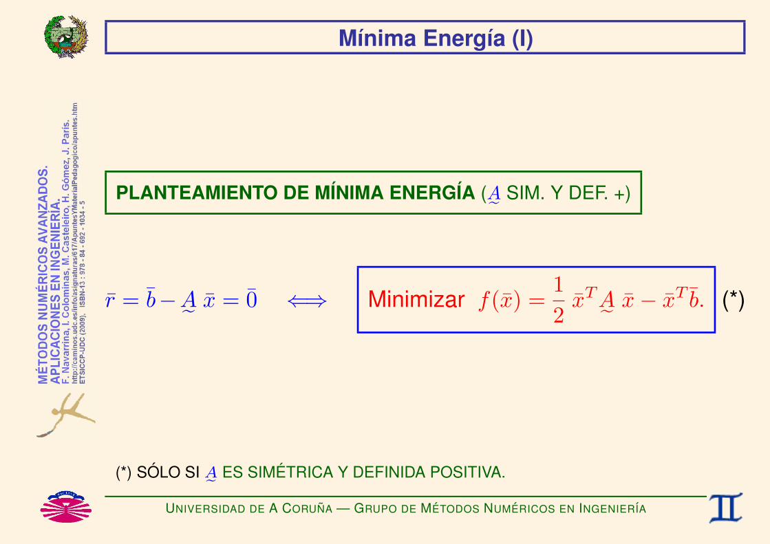
Mınima Energıa (I)
PLANTEAMIENTO DE MINIMA ENERGIA (A˜ SIM. Y DEF. +)
r = b−A˜ x = 0 ⇐⇒ Minimizar f(x) =12
xTA˜ x− xT b. (*)
(*) SOLO SI Ae ES SIMETRICA Y DEFINIDA POSITIVA.
UNIVERSIDAD DE A CORUNA — GRUPO DE METODOS NUMERICOS EN INGENIERIA

Mınima Energıa (II)
VECTORES DE PRUEBA
Sean los vectores de prueba L.I.φi
i=1,...,ν
, ν ≤ n.
Dada la aproximacion inicial x0, buscamos una mejor aproximacion
x ≈ xh = x0 +ν∑
i=1
αiφi
x ≈ xh = x0 + Φ˜ α, con Φ˜ = [ φ1 . . . φν ] , α =
α1...
αν
.
El residuo correspondiente a la aproximacion xh sera
rh = b−A˜(
x0 +ν∑
i=1
αiφi
)= r0 −
ν∑i=1
αi
(A˜ φi
)rh = b−A˜ (x0 + Φ˜ α) = r0 −A˜ Φ˜ α
UNIVERSIDAD DE A CORUNA — GRUPO DE METODOS NUMERICOS EN INGENIERIA

Mınima Energıa (IIIa)
Sea
ϕ(α) = f(x)∣∣∣x=xh
=12(xh)T
A˜ xh −(xh)T
b.
Nos proponemos obtener la aproximacion xh que verifique
∂ϕ
∂αj= 0, j=1,...,ν ⇐⇒
[dϕ
dα
]T
= 0.
UNIVERSIDAD DE A CORUNA — GRUPO DE METODOS NUMERICOS EN INGENIERIA
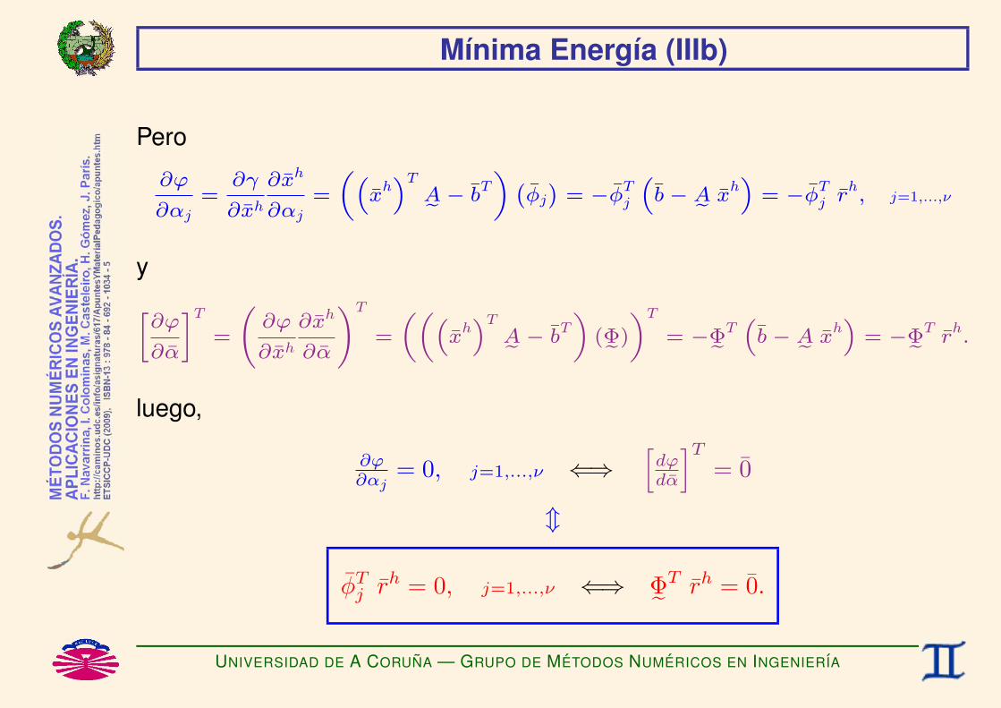
Mınima Energıa (IIIb)
Pero
∂ϕ
∂αj
=∂γ
∂xh
∂xh
∂αj
=
„“x
h”T
Ae − bT
«`φj
´= −φ
Tj
“b− Ae x
h”
= −φTj r
h, j=1,...,ν
y
»∂ϕ
∂α
–T
=
∂ϕ
∂xh
∂xh
∂α
!T
=
„„“x
h”T
Ae − bT
«(Φe)
«T
= −ΦeT“
b− Ae xh”
= −ΦeTr
h.
luego,
∂ϕ∂αj
= 0, j=1,...,ν ⇐⇒[
dϕdα
]T= 0
m
φTj rh = 0, j=1,...,ν ⇐⇒ Φ˜T rh = 0.
UNIVERSIDAD DE A CORUNA — GRUPO DE METODOS NUMERICOS EN INGENIERIA

Mınima Energıa (IVa)
Por tanto,
φTj
r0 −
νXi=1
αi
`Ae φi
´!= 0, j=1,...,ν ⇐⇒ ΦeT (r0 − Ae Φe α) = 0
m
νXi=1
kjiz | “φ
Tj Ae φi
”αi =
fjz | φ
Tj r0, j=1,...,ν ⇐⇒
Kez | “ΦeT
Ae Φe”
α =
fz | ΦeT
r0
m
νXi=1
kjiαi = fj, j=1,...,ν ⇐⇒ Ke α = f .
UNIVERSIDAD DE A CORUNA — GRUPO DE METODOS NUMERICOS EN INGENIERIA
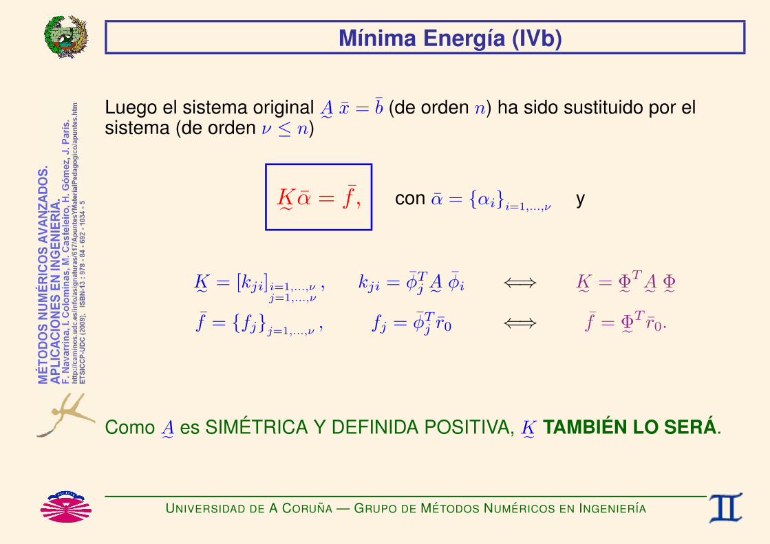
Mınima Energıa (IVb)
Luego el sistema original A˜ x = b (de orden n) ha sido sustituido por elsistema (de orden ν ≤ n)
K˜ α = f , con α = αii=1,...,νy
K˜ = [kji]i=1,...,νj=1,...,ν
, kji = φTj A˜ φi ⇐⇒ K˜ = Φ˜TA˜ Φ˜
f = fjj=1,...,ν, fj = φT
j r0 ⇐⇒ f = Φ˜T r0.
Como A˜ es SIMETRICA Y DEFINIDA POSITIVA, K˜ TAMBIEN LO SERA.
UNIVERSIDAD DE A CORUNA — GRUPO DE METODOS NUMERICOS EN INGENIERIA

Mınima Energıa (V)
Luego el PLANTEAMIENTO DE MINIMA ENERGIA . . .
♣ es un metodo de RESIDUOS PONDERADOS,
♣ en el que se utilizan los vectores de test
ωj = φj, j=1,...,ν ⇐⇒ Ω˜ = Φ˜Por tanto se utiliza una ponderacion del tipo BUBNOV–GALERKIN. (*)
(*) En este caso.
UNIVERSIDAD DE A CORUNA — GRUPO DE METODOS NUMERICOS EN INGENIERIA

Metodos de Krylov (I)
SUBESPACIO DE KRYLOV
Dados A˜ y ro, se define el subespacio de Krylov Km(A˜ , ro) como
Km(A˜ , ro) = spanro, A˜ ro, A˜2ro, . . . , A˜m−1ro
=
xm
∣∣∣ xm =n∑
i=1
αiA˜ i−1ro
.
METODOS DE KRYLOV
Dada la aproximacion inicial x0, buscamos una mejor aproximacion
x ≈ xh = x0 + xm, con xm ∈ Km(A˜ , ro).
La obtencion de la mejor aproximacion se plantea mediante el metodo deresiduos ponderados.
UNIVERSIDAD DE A CORUNA — GRUPO DE METODOS NUMERICOS EN INGENIERIA

Metodos de Krylov (II)
Luego los METODOS DE KRYLOV . . .
♣ son metodos de RESIDUOS PONDERADOS,
♣ en los que se utilizan los vectores de prueba
φi = A˜ i−1ro, i=1,...,m.
UNIVERSIDAD DE A CORUNA — GRUPO DE METODOS NUMERICOS EN INGENIERIA
Metodos de Krylov (III)
En particular, puede comprobarse facilmente (*) que elMETODO DE GRADIENTES CONJUGADOS . . .
♣ es un METODO DE KRYLOV.
(*) Basta examinar como se van generando las sucesivas aproximaciones a la solucion.
UNIVERSIDAD DE A CORUNA — GRUPO DE METODOS NUMERICOS EN INGENIERIA

Matrices no simetricas
Si A˜ es no simetrica, podemos utilizar . . .
1) El Metodo de Mınimos Cuadrados (o de Mınimo Residuo).♦ Es facil modificar el PCG (basta trabajar con lo residuos br = AeT r,
♣ pero el numero de condicion de AeTAe es el cuadrado del numero de condicion de lamatriz original Ae , por lo que♠ se esperan errores de redondeo mas importantes y♠ se espera una menor velocidad de convergencia (*).
2) El Metodo de Mınimo Residuo Generalizado (GMRES).♥ Se realizan ciertas correcciones que evitan los problemas del metodo anterior,♣ pero a cambio es preciso retener todas los iteraciones (no solo la ultima),
♠ lo que implica un volumen de almacenamiento en memoria inaceptable.
♣ Para evitarlo, el metodo se arranca de nuevo cada cierto numero de iteraciones,♠ pero entonces puede no converger.
(*) Puede demostrarse que el numero de iteraciones necesarias para obtener una buena aproximacion crece con la raızcuadrada del numero de condicion de la matriz (vease, por ejemplo, C. Johnson, 1992).
UNIVERSIDAD DE A CORUNA — GRUPO DE METODOS NUMERICOS EN INGENIERIA

METODOS SEMI-ITERATIVOS PARAGRANDES SISTEMAS DE ECUACIONES LINEALES:PLANTEAMIENTO EN RESIDUOS ELEMENTALESF. Navarrina, I. Colominas, M. Casteleiro, H. Gomez, J. Parıs
GMNI — GRUPO DE METODOS NUMERICOS EN INGENIERIA
Departamento de Metodos Matematicos y de RepresentacionEscuela Tecnica Superior de Ingenieros de Caminos, Canales y Puertos
Universidad de A Coruna, Espana
e-mail: [email protected] web: http://caminos.udc.es/gmni
UNIVERSIDAD DE A CORUNA — GRUPO DE METODOS NUMERICOS EN INGENIERIA

INDICE
I Ensamblaje de la diagonal principal
I Calculo del residuo a nivel de elemento
UNIVERSIDAD DE A CORUNA — GRUPO DE METODOS NUMERICOS EN INGENIERIA

Ensamblaje de la diagonal principal (I)
La diag (K˜ ) se obtiene ensamblando las diag (K˜ e), pues
K˜ =nelem∑e=1
K˜ e =⇒ diag (K˜ ) =nelem∑e=1
diag(K˜ e
).
UNIVERSIDAD DE A CORUNA — GRUPO DE METODOS NUMERICOS EN INGENIERIA

Ensamblaje de la diagonal principal (II)
Siendo
K˜ e =[ke
ij
], con
i = 1, . . . , nevab
j = 1, . . . , nevab
los coeficientes de diag (K˜ e) pueden calcularse en la forma
kejj = δT
e,j K˜ e δe,j, con δe,j =
0...01 −→ fila j0......0
UNIVERSIDAD DE A CORUNA — GRUPO DE METODOS NUMERICOS EN INGENIERIA

Ensamblaje de la diagonal principal (III)
Pero
K˜ e = B˜Te D˜ eB˜ e,
luego
kejj = δT
e,j K˜ e δe,j = δTe,j
(B˜T
e D˜ eB˜ e
)δe,j
=(δTe,j B˜T
e
)D˜ e
(B˜ e δe,j
)=
(B˜ e δe,j
)TD˜ e
(B˜ e δe,j
),
y por tanto
ue,j = δe,j
εe,j = B˜ e ue,j
σe,j = D˜ e εe,j
=⇒ kejj = (εe,j)
Tσe,j .
UNIVERSIDAD DE A CORUNA — GRUPO DE METODOS NUMERICOS EN INGENIERIA

Calculo del residuo a nivel de elemento (I)
El residuo r se obtiene ensamblando las contribuciones fe = K˜ eue, pues
r = b−K˜ u
K˜ =nelem∑e=1
K˜ e
=⇒ r = b−nelem∑e=1
K˜ eu︸︷︷︸bfe
,
donde la contribucion fe se obtiene expandiendo
fe = K˜ eue.
UNIVERSIDAD DE A CORUNA — GRUPO DE METODOS NUMERICOS EN INGENIERIA
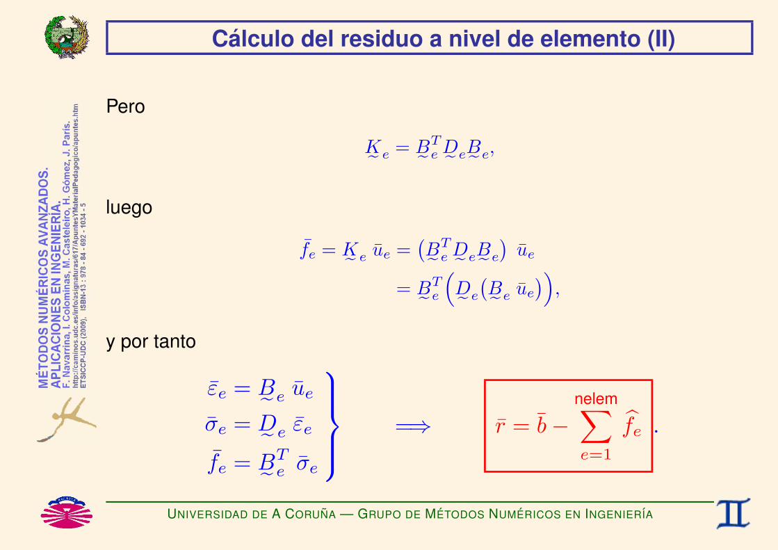
Calculo del residuo a nivel de elemento (II)
Pero
K˜ e = B˜Te D˜ eB˜ e,
luego
fe = K˜ e ue =(B˜T
e D˜ eB˜ e
)ue
= B˜Te
(D˜ e
(B˜ e ue
)),
y por tanto
εe = B˜ e ue
σe = D˜ e εe
fe = B˜Te σe
=⇒ r = b−nelem∑e=1
fe .
UNIVERSIDAD DE A CORUNA — GRUPO DE METODOS NUMERICOS EN INGENIERIA


INTRODUCCION A LOSMETODOS DE RESIDUOS PONDERADOS:
APROXIMACION DE FUNCIONESF. Navarrina, I. Colominas, M. Casteleiro, H. Gomez, J. Parıs
GMNI — GRUPO DE METODOS NUMERICOS EN INGENIERIA
Departamento de Metodos Matematicos y de RepresentacionEscuela Tecnica Superior de Ingenieros de Caminos, Canales y Puertos
Universidad de A Coruna, Espana
e-mail: [email protected] web: http://caminos.udc.es/gmni
UNIVERSIDAD DE A CORUNA — GRUPO DE METODOS NUMERICOS EN INGENIERIA

INDICE
I Planteamientos Alternativos
I Residuos Ponderados
I Eleccion de las Funciones de Test
I Metodo de Colocacion Puntual
I Metodo de Colocacion por Subdominios
I Metodo de Bubnov-Galerkin
I Eleccion de las Funciones de Prueba
I Metodo de Mınimos Cuadrados
I Notacion en Formas Bilineales
UNIVERSIDAD DE A CORUNA — GRUPO DE METODOS NUMERICOS EN INGENIERIA

Planteamientos Alternativos (I)
Sea el problema:
Hallar u(x), x ∈ [a, b]
que verifica u(x) = f(x) ∀x ∈ [a, b].
El problema anterior puede escribirse en las formas alternativas...
UNIVERSIDAD DE A CORUNA — GRUPO DE METODOS NUMERICOS EN INGENIERIA

Planteamientos Alternativos (IIa)
a) FORMA ORIGINAL
Hallar u(x), x ∈ [a, b],
que VERIFICA r(x) = 0 ∀x ∈ [a, b], (*)
siendo r(x) = f(x)− u(x).
(*) FORMA FUERTE o STRONG FORM.
UNIVERSIDAD DE A CORUNA — GRUPO DE METODOS NUMERICOS EN INGENIERIA

Planteamientos Alternativos (IIb1)
b) RESIDUOS PONDERADOS
Hallar u(x), x ∈ [a, b],
que VERIFICA
∫ b
a
ω(x)r(x) dx = 0 ∀ω(x), (*)
siendo r(x) = f(x)− u(x).
(*) FORMA DEBIL o WEAK FORM.
UNIVERSIDAD DE A CORUNA — GRUPO DE METODOS NUMERICOS EN INGENIERIA
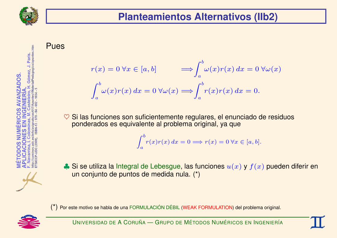
Planteamientos Alternativos (IIb2)
Pues
r(x) = 0 ∀x ∈ [a, b] =⇒Z b
a
ω(x)r(x) dx = 0 ∀ω(x)Z b
a
ω(x)r(x) dx = 0 ∀ω(x) =⇒Z b
a
r(x)r(x) dx = 0.
♥ Si las funciones son suficientemente regulares, el enunciado de residuosponderados es equivalente al problema original, ya queZ b
ar(x)r(x) dx = 0 =⇒ r(x) = 0 ∀x ∈ [a, b].
♣ Si se utiliza la Integral de Lebesgue, las funciones u(x) y f(x) pueden diferir enun conjunto de puntos de medida nula. (*)
(*) Por este motivo se habla de una FORMULACION DEBIL (WEAK FORMULATION) del problema original.
UNIVERSIDAD DE A CORUNA — GRUPO DE METODOS NUMERICOS EN INGENIERIA
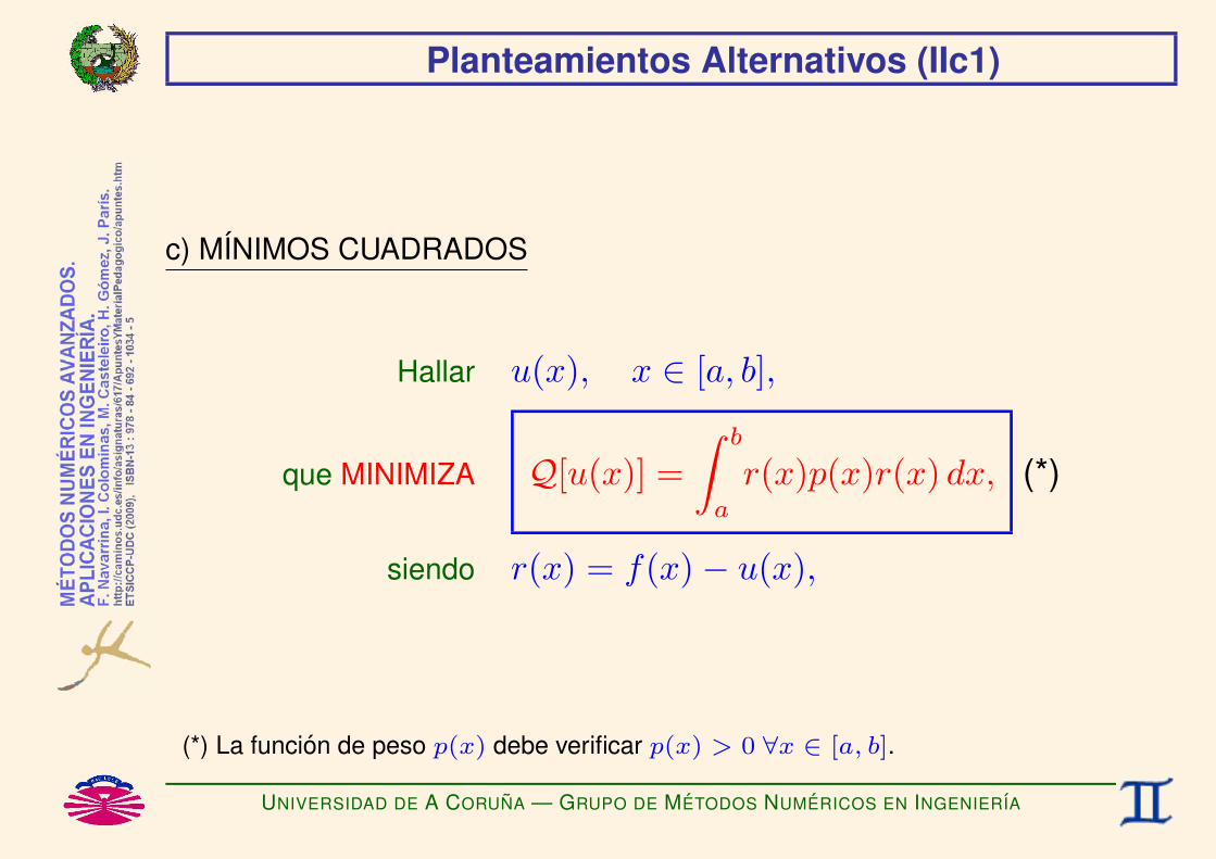
Planteamientos Alternativos (IIc1)
c) MINIMOS CUADRADOS
Hallar u(x), x ∈ [a, b],
que MINIMIZA Q[u(x)] =∫ b
a
r(x)p(x)r(x) dx, (*)
siendo r(x) = f(x)− u(x),
(*) La funcion de peso p(x) debe verificar p(x) > 0 ∀x ∈ [a, b].
UNIVERSIDAD DE A CORUNA — GRUPO DE METODOS NUMERICOS EN INGENIERIA

Planteamientos Alternativos (IIc2)
que equivale al PLANTEAMIENTO VARIACIONAL
Hallar u(x), x ∈ [a, b],
que VERIFICAdJ(λ)
dλ
∣∣∣∣λ=0
= 0 ∀δu(x),
siendo J(λ) =
Z b
a
“r(x)− λδu(x)
”p(x)
“r(x)− λδu(x)
”dx, (*)
y por tantodJ(λ)
dλ
∣∣∣∣λ=0
= −2∫ b
a
δu(x)p(x)r(x) dx,
r(x) = f(x)− u(x),
(*) La funcion de peso p(x) debe verificar p(x) > 0 ∀x ∈ [a, b].
UNIVERSIDAD DE A CORUNA — GRUPO DE METODOS NUMERICOS EN INGENIERIA
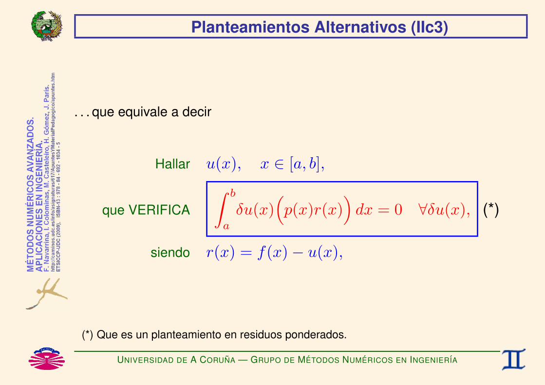
Planteamientos Alternativos (IIc3)
. . . que equivale a decir
Hallar u(x), x ∈ [a, b],
que VERIFICA
∫ b
a
δu(x)(p(x)r(x)
)dx = 0 ∀δu(x), (*)
siendo r(x) = f(x)− u(x),
(*) Que es un planteamiento en residuos ponderados.
UNIVERSIDAD DE A CORUNA — GRUPO DE METODOS NUMERICOS EN INGENIERIA

Planteamientos Alternativos (IIc4)
. . . o lo que es lo mismo
Hallar u(x), x ∈ [a, b],
que VERIFICA
∫ b
a
ω(x)r(x) dx = 0 ∀ω(x) = δu(x)p(x), (*)
siendo r(x) = f(x)− u(x).
(*) Que es un planteamiento en residuos ponderados.
UNIVERSIDAD DE A CORUNA — GRUPO DE METODOS NUMERICOS EN INGENIERIA

Planteamientos Alternativos (IId1)
e) MINIMA ENERGIA
Hallar u(x), x ∈ [a, b],
que MINIMIZA E [u(x)] =12
∫ b
a
u(x)u(x) dx−∫ b
a
u(x)f(x) dx,
UNIVERSIDAD DE A CORUNA — GRUPO DE METODOS NUMERICOS EN INGENIERIA
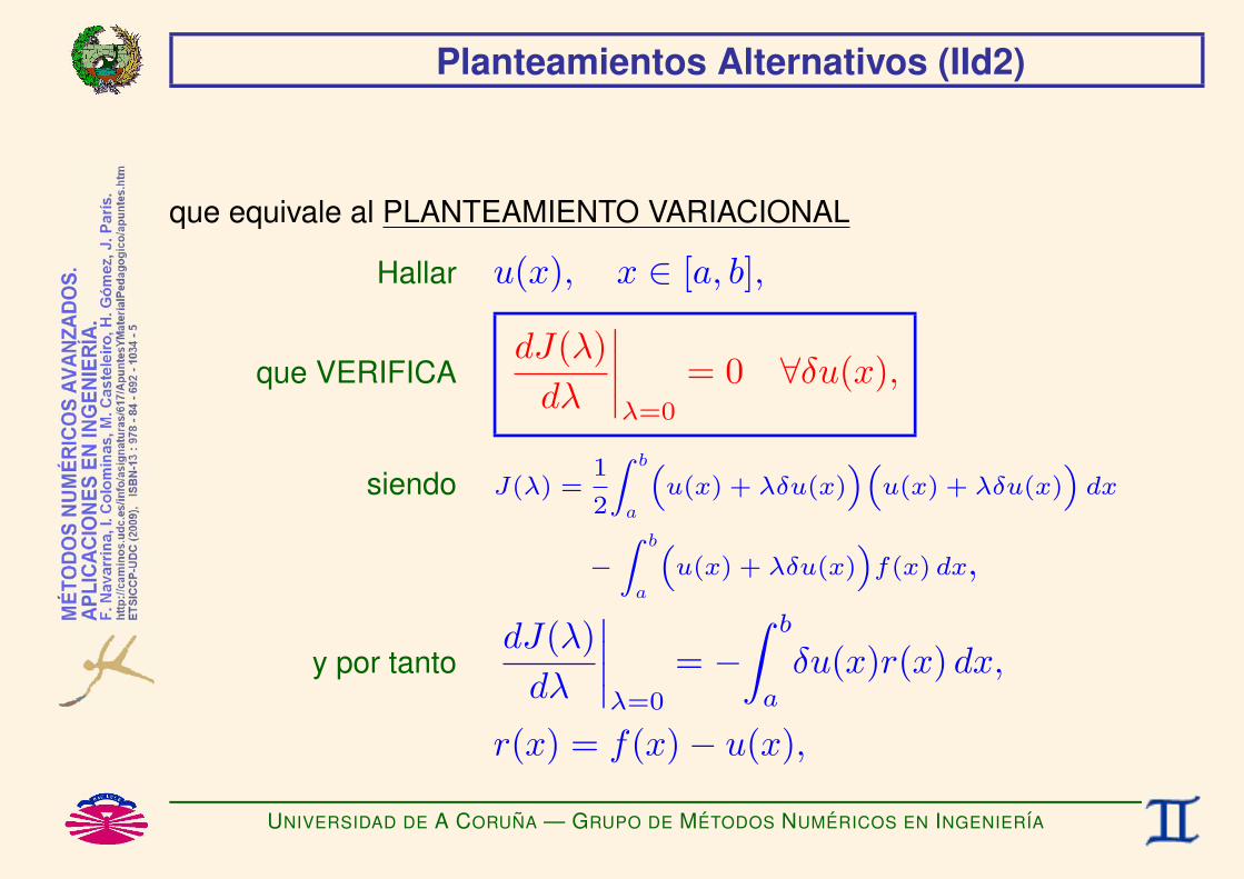
Planteamientos Alternativos (IId2)
que equivale al PLANTEAMIENTO VARIACIONAL
Hallar u(x), x ∈ [a, b],
que VERIFICAdJ(λ)
dλ
∣∣∣∣λ=0
= 0 ∀δu(x),
siendo J(λ) =1
2
Z b
a
“u(x) + λδu(x)
”“u(x) + λδu(x)
”dx
−Z b
a
“u(x) + λδu(x)
”f(x) dx,
y por tantodJ(λ)
dλ
∣∣∣∣λ=0
= −∫ b
a
δu(x)r(x) dx,
r(x) = f(x)− u(x),
UNIVERSIDAD DE A CORUNA — GRUPO DE METODOS NUMERICOS EN INGENIERIA

Planteamientos Alternativos (IId3)
. . . que equivale a decir
Hallar u(x), x ∈ [a, b],
que VERIFICA
∫ b
a
δu(x)r(x) dx = 0 ∀δu(x), (*)
siendo r(x) = f(x)− u(x),
(*) Que es un planteamiento en residuos ponderados.
UNIVERSIDAD DE A CORUNA — GRUPO DE METODOS NUMERICOS EN INGENIERIA
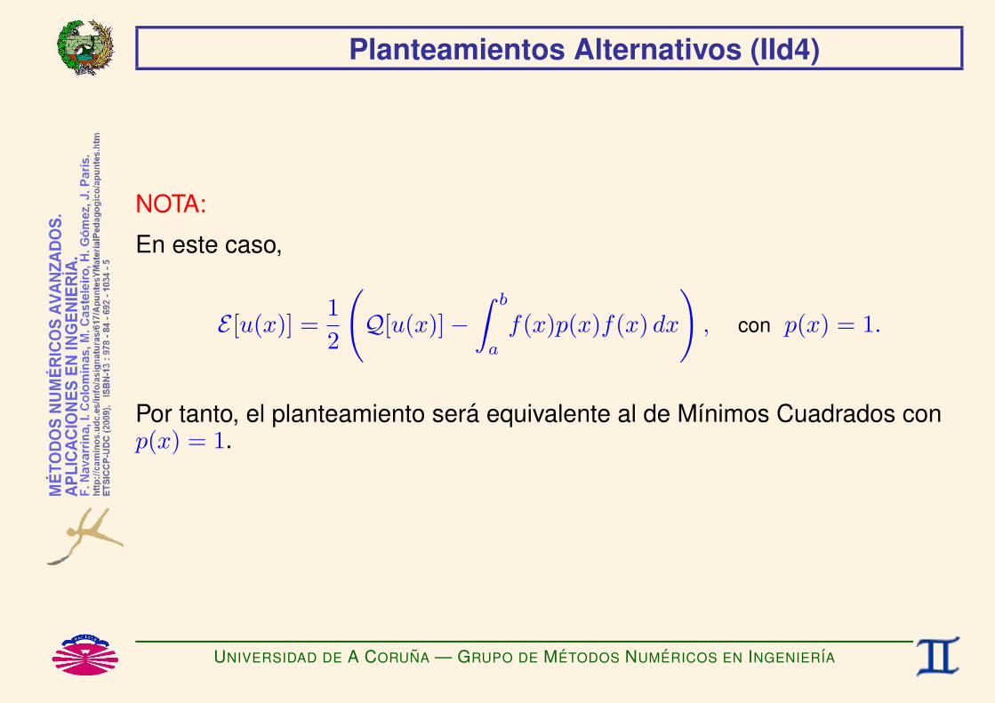
Planteamientos Alternativos (IId4)
NOTA:
En este caso,
E [u(x)] =12
(Q[u(x)]−
∫ b
a
f(x)p(x)f(x) dx
), con p(x) = 1.
Por tanto, el planteamiento sera equivalente al de Mınimos Cuadrados conp(x) = 1.
UNIVERSIDAD DE A CORUNA — GRUPO DE METODOS NUMERICOS EN INGENIERIA

Residuos Ponderados (I)
RESIDUOS PONDERADOS (Weighted Residuals)
Hallar u(x) ∈ Hu,
que VERIFICA
∫ b
a
ω(x)r(x) dx = 0 ∀ω(x) ∈ Hω,
siendo r(x) = f(x)− u(x).
UNIVERSIDAD DE A CORUNA — GRUPO DE METODOS NUMERICOS EN INGENIERIA
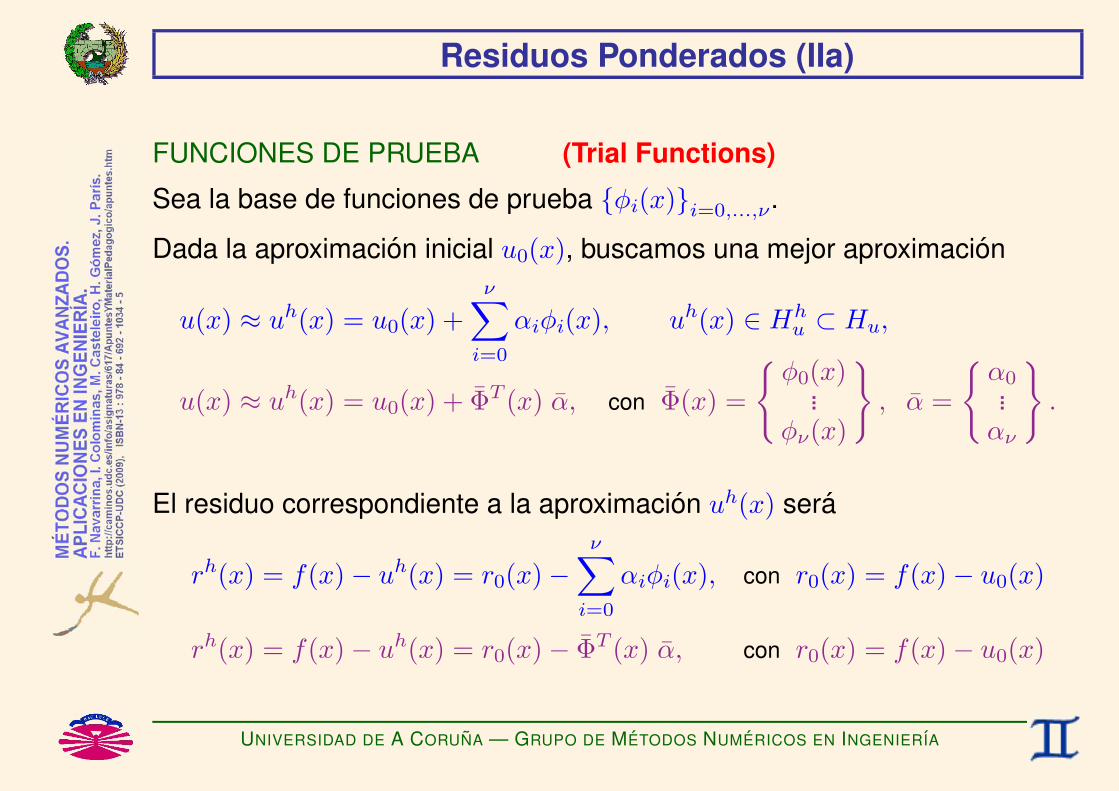
Residuos Ponderados (IIa)
FUNCIONES DE PRUEBA (Trial Functions)
Sea la base de funciones de prueba φi(x)i=0,...,ν.
Dada la aproximacion inicial u0(x), buscamos una mejor aproximacion
u(x) ≈ uh(x) = u0(x) +ν∑
i=0
αiφi(x), uh(x) ∈ Hhu ⊂ Hu,
u(x) ≈ uh(x) = u0(x) + ΦT (x) α, con Φ(x) =
φ0(x)
...φν(x)
, α =
α0...αν
.
El residuo correspondiente a la aproximacion uh(x) sera
rh(x) = f(x)− uh(x) = r0(x)−ν∑
i=0
αiφi(x), con r0(x) = f(x)− u0(x)
rh(x) = f(x)− uh(x) = r0(x)− ΦT (x) α, con r0(x) = f(x)− u0(x)
UNIVERSIDAD DE A CORUNA — GRUPO DE METODOS NUMERICOS EN INGENIERIA

Residuos Ponderados (IIb)
En general no sera posible que uh(x) = u(x) ∀x ∈ [a, b] (*), por lo que
rh(x) 6= 0 =⇒ no es posible que
∫ b
a
ω(x)rh(x) dx = 0 ∀ω(x) ∈ Hω.
(*) Salvo que u(x)− u0(x) este contenido en el subespacio generado por las funciones de prueba.
UNIVERSIDAD DE A CORUNA — GRUPO DE METODOS NUMERICOS EN INGENIERIA
Residuos Ponderados (IIIa)
FUNCIONES DE TEST (Test Functions)
Sea la base de funciones de test ωj(x)j=0,...,ν.
Sea
ωh(x) =ν∑
j=0
βjωj(x), ωh(x) ∈ Hhω ⊂ Hω,
ωh(x) = ΩT (x) β = βT Ω(x), con Ω(x) =
ω0(x)
...ων(x)
, β =
β0...βν
.
Nos proponemos obtener la aproximacion uh(x) ∈ Hhu que verifique
∫ b
a
ωh(x)rh(x) dx = 0 ∀ωh(x) ∈ Hhω.
UNIVERSIDAD DE A CORUNA — GRUPO DE METODOS NUMERICOS EN INGENIERIA

Residuos Ponderados (IIIb)
Pero Z b
a
ωh(x)r
h(x) dx = 0 ∀ω
h(x) ∈ H
hω
mZ b
a
0@ νXj=0
βjωj(x)
1Arh(x) dx = 0 ∀ βj ⇐⇒
Z b
a
“β
TΩ(x)
”r
h(x) dx = 0 ∀β
mνX
j=0
βj
Z b
a
ωj(x)rh(x) dx = 0 ∀ βj ⇐⇒ β
TZ b
a
Ω(x)rh(x) dx = 0 ∀β
m
Z b
a
ωj(x)rh(x) dx = 0, j=0,...,ν ⇐⇒
Z b
a
Ω(x)rh(x) dx = 0.
UNIVERSIDAD DE A CORUNA — GRUPO DE METODOS NUMERICOS EN INGENIERIA

Residuos Ponderados (IVa)
Por tanto,
Z b
aωj(x)
r0(x)−
νXi=0
αiφi(x)
!= 0 ∀j ⇐⇒
Z b
aΩ(x)
“r0(x)− Φ
T(x) α
”dx = 0
m
νXi=0
kjiz | Z b
aωj(x)φi(x) dx αi =
fjz | Z b
aωj(x)r0(x) dx ∀j ⇐⇒
Kez | Z b
aΩ(x) Φ
T(x) dx α =
fz | Z b
aΩ(x)r0(x) dx
m
νXi=0
kjiαi = fj j=0,...,ν ⇐⇒ Ke α = f .
UNIVERSIDAD DE A CORUNA — GRUPO DE METODOS NUMERICOS EN INGENIERIA
Residuos Ponderados (IVb)
Luego el problema original u(x) = f(x) ha sido sustituido por el sistema (deorden ν + 1)
K˜ α = f , con α = αii=0,...,νy
Ke = [kji]i=0,...,νj=0,...,ν
, kji =
Z b
a
ωj(x)φi(x) dx ⇐⇒ Ke =
Z b
a
Ω(x)ΦT (x) dx
f = fjj=0,...,ν , fj =
Z b
a
ωj(x)r0(x) dx ⇐⇒ f =
Z b
a
Ω(x)r0(x) dx.
Posteriormente obtendremos la aproximacion a la solucion
uh(x) = u0(x) +ν∑
i=0
αiφi(x) ⇐⇒ uh(x) = u0(x) + ΦT (x) α.
UNIVERSIDAD DE A CORUNA — GRUPO DE METODOS NUMERICOS EN INGENIERIA

Residuos Ponderados (Va)
METODOS DE PROYECCION
Los METODOS DE RESIDUOS PONDERADOS tambien se denominan ası,
ya que siendo
u(x) la solucion exacta, con r(x) = f(x)− u(x)
uh(x) la solucion aproximada, con rh(x) = f(x)− uh(x)
se verificaZ b
aω
h(x)r(x) dx = 0 ∀ω
h(x) ∈ H
hω
Z b
aω
h(x)r
h(x) dx = 0 ∀ω
h(x) ∈ H
hω
9>>>>>=>>>>>;=⇒
Z b
aω
h(x)“
r(x)− rh(x)”
dx = 0 ∀ωh(x) ∈ H
hω
=⇒−Z b
aω
h(x)“
u(x)− uh(x)”
dx = 0 ∀ωh(x) ∈ H
hω.
UNIVERSIDAD DE A CORUNA — GRUPO DE METODOS NUMERICOS EN INGENIERIA

Residuos Ponderados (Vb)
Luego, la solucion aproximada uh(x) verifica
⟨ωh, u− uh
⟩= 0 ∀ωh(x) ∈ Hh
ω, con 〈v, e〉 =∫ b
a
v(x)e(x) dx.
Por tanto, . . .
UNIVERSIDAD DE A CORUNA — GRUPO DE METODOS NUMERICOS EN INGENIERIA

Residuos Ponderados (Vc)
. . . la solucion aproximada uh(x) es
la PROYECCION de la solucion exacta u(x)
sobre el subespacio Hhu de las funciones de prueba uh(x)
segun la normal al subespacio Hhω de las funciones de test ωh(x).
UNIVERSIDAD DE A CORUNA — GRUPO DE METODOS NUMERICOS EN INGENIERIA

Eleccion de las Funciones de Test
Algunas posibilidades. . .
1) METODO DE COLOCACION PUNTUAL
ωj(x) = δ(x− xj), j=0,...,ν con xj∈[a,b], xi 6=xj ∀i6=j. (*)
2) METODO DE COLOCACION POR SUBDOMINIOS
ωj(x) = 1, si xj ≤ x ≤ xj+1,
0, en caso contrario, j=0,...,ν con a=x0≤x1≤...≤xν≤xν+1=b.
3) METODO DE BUBNOV-GALERKIN
ωj(x) = φj(x), j=0,...,ν ⇐⇒ Hhω = Hh
u .
(*) Si xj = a o xj = b es preciso redefinir adecuadamente la δ.
UNIVERSIDAD DE A CORUNA — GRUPO DE METODOS NUMERICOS EN INGENIERIA
Metodo de Colocacion Puntual (Ia)
COLOCACION PUNTUAL
Si se eligen como funciones de test las deltas de Dirac
ωj(x) = δ(x− xj), j=0,...,ν con xj∈[a,b], xi 6=xj ∀i6=j,
se obtiene
Ke = [kji]i=0,...,νj=0,...,ν
, kji =
Z b
a
ωj(x)φi(x) dx = φi(xj)
f = fjj=0,...,ν , fj =
Z b
a
ωj(x)r0(x) dx = r0(xj) = f(xj)− u0(xj).
UNIVERSIDAD DE A CORUNA — GRUPO DE METODOS NUMERICOS EN INGENIERIA
Metodo de Colocacion Puntual (Ib)
Esto es 2664φ0(x0) φ1(x0) . . . φν(x0)φ0(x1) φ1(x1) . . . φν(x1)... ... ...φ0(xν) φ1(xν) . . . φν(xν)
37758><>:
α0
α1...αν
9>=>; =
=
8>><>>:f(x0)− u0(x0)f(x1)− u0(x1)...f(xν)− u0(xν)
9>>=>>; .
UNIVERSIDAD DE A CORUNA — GRUPO DE METODOS NUMERICOS EN INGENIERIA

Metodo de Colocacion Puntual (II)
La solucion aproximada uh(x) verifica∫ b
a
ωj(x)rh(x) dx =∫ b
a
δ(x− xj)rh(x) dx = rh(xj) = 0
⇓
uh(xj) = f(xj), j = 0, . . . , ν.
por lo que se realiza una INTERPOLACION PURA.
UNIVERSIDAD DE A CORUNA — GRUPO DE METODOS NUMERICOS EN INGENIERIA

Metodo de Colocacion por Subdominios (Ia)
COLOCACION POR SUBDOMINIOS
Si se eligen como funciones de test las funciones en escalon
ωj(x) = 1, si xj ≤ x ≤ xj+1,
0, en caso contrario, j=0,...,ν con a=x0≤x1≤...≤xν≤xν+1=b.
se obtiene
Ke = [kji]i=0,...,νj=0,...,ν
, kji =
Z b
a
ωj(x)φi(x) dx =R xj+1
xjφi(x) dx
f = fjj=0,...,ν , fj =
Z b
a
ωj(x)r0(x) dx =R xj+1
xj[f(x)− u0(x)] dx.
UNIVERSIDAD DE A CORUNA — GRUPO DE METODOS NUMERICOS EN INGENIERIA

Metodo de Colocacion por Subdominios (Ib)
Esto es2666666664
Z x1
x0
φ0(x) dx
Z x1
x0
φ1(x) dx . . .
Z x1
x0
φν(x) dxZ x2
x1
φ0(x) dx
Z x2
x1
φ1(x) dx . . .
Z x2
x1
φν(x) dx
... ... ...Z xν+1
xν
φ0(x) dx
Z xν+1
xν
φ1(x) dx . . .
Z xν+1
xν
φν(x) dx
37777777758><>:
α0
α1...αν
9>=>; =
=
8>>>>>>>><>>>>>>>>:
Z x1
x0
[f(x)− u0(x)] dxZ x2
x1
[f(x)− u0(x)] dx
...Z xν+1
xν
[f(x)− u0(x)] dx
9>>>>>>>>=>>>>>>>>;.
UNIVERSIDAD DE A CORUNA — GRUPO DE METODOS NUMERICOS EN INGENIERIA

Metodo de Colocacion por Subdominios (II)
La solucion aproximada uh(x) verifica∫ b
a
ωj(x)rh(x) dx =∫ xj+1
xj
rh(x) dx = 0
⇓
∫ xj+1
xj
uh(x) dx =∫ xj+1
xj
f(x) dx, j = 0, . . . , ν
por lo que se realiza un AJUSTE DE LA MEDIA POR INTERVALOS.
UNIVERSIDAD DE A CORUNA — GRUPO DE METODOS NUMERICOS EN INGENIERIA
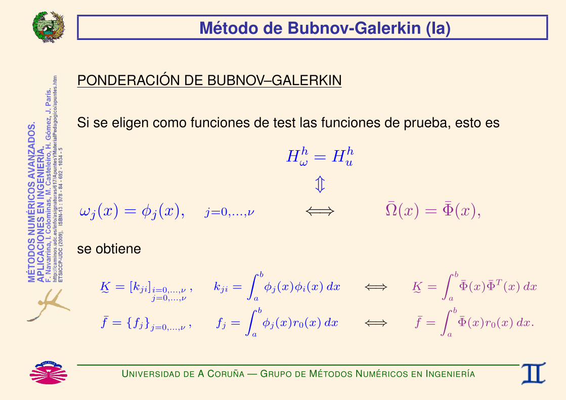
Metodo de Bubnov-Galerkin (Ia)
PONDERACION DE BUBNOV–GALERKIN
Si se eligen como funciones de test las funciones de prueba, esto es
Hhω = Hh
u
mωj(x) = φj(x), j=0,...,ν ⇐⇒ Ω(x) = Φ(x),
se obtiene
Ke = [kji]i=0,...,νj=0,...,ν
, kji =
Z b
a
φj(x)φi(x) dx ⇐⇒ Ke =
Z b
a
Φ(x)ΦT (x) dx
f = fjj=0,...,ν , fj =
Z b
a
φj(x)r0(x) dx ⇐⇒ f =
Z b
a
Φ(x)r0(x) dx.
UNIVERSIDAD DE A CORUNA — GRUPO DE METODOS NUMERICOS EN INGENIERIA

Metodo de Bubnov-Galerkin (Ib)
Esto es2666666664
Z b
a
φ0(x)φ0(x) dx
Z b
a
φ0(x)φ1(x) dx . . .
Z b
a
φ0(x)φν(x) dxZ b
a
φ1(x)φ0(x) dx
Z b
a
φ1(x)φ1(x) dx . . .
Z b
a
φ1(x)φν(x) dx
... ... ...Z b
a
φν(x)φ0(x) dx
Z b
a
φν(x)φ1(x) dx . . .
Z b
a
φν(x)φν(x) dx
37777777758><>:
α0
α1...αν
9>=>; =
=
8>>>>>>>><>>>>>>>>:
Z b
a
φ0(x) [f(x)− u0(x)] dxZ b
a
φ1(x) [f(x)− u0(x)] dx
...Z b
a
φν(x) [f(x)− u0(x)] dx
9>>>>>>>>=>>>>>>>>;. (*)
(*) Ecuaciones normales de Euler.
UNIVERSIDAD DE A CORUNA — GRUPO DE METODOS NUMERICOS EN INGENIERIA

Metodo de Bubnov-Galerkin (II)
La solucion aproximada uh(x) verifica∫ b
a
ωj(x)rh(x) dx =∫ b
a
φj(x)rh(x) dx = 0
⇓
∂Q
∂αj= 0, siendo Q(α0, α1, . . . , αν) =
∫ b
a
(rh(x)
)2
dx,
por lo que se realiza un AJUSTE POR MINIMOS CUADRADOS.
UNIVERSIDAD DE A CORUNA — GRUPO DE METODOS NUMERICOS EN INGENIERIA
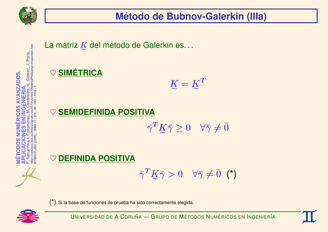
Metodo de Bubnov-Galerkin (IIIa)
La matriz K˜ del metodo de Galerkin es. . .
♥ SIMETRICAK˜ = K˜ T
♥ SEMIDEFINIDA POSITIVA
γTK˜ γ ≥ 0 ∀γ 6= 0
♥ DEFINIDA POSITIVA
γTK˜ γ > 0 ∀γ 6= 0 (*)
(*) Si la base de funciones de prueba ha sido correctamente elegida.
UNIVERSIDAD DE A CORUNA — GRUPO DE METODOS NUMERICOS EN INGENIERIA

Metodo de Bubnov-Galerkin (IIIb)
K˜ es SIMETRICA, ya que
kji =
Z b
a
φj(x)φi(x) dx =
Z b
a
φi(x)φj(x) dx = kij
m
Ke =
Z b
a
Φ(x)ΦT(x) dx =
Z b
a
“Φ(x)Φ
T(x)”T
dx =
Z b
a
Φ(x)ΦT(x) dx
!T
= Ke T.
UNIVERSIDAD DE A CORUNA — GRUPO DE METODOS NUMERICOS EN INGENIERIA

Metodo de Bubnov-Galerkin (IIIc)
K˜ es SEMIDEFINIDA POSITIVA, ya que
νXj=0
νXi=0
γjkjiγi =νX
j=0
νXi=0
γj
Z b
aφj(x)φi(x) dx
!γi =
Z b
a
0@ νXj=0
γjφj(x)
1A| z
g(x)
νX
i=0
γiφi(x)
!| z
g(x)
dx
=
Z b
a
νX
i=0
γiφi(x)
!2
dx ≥ 0 ∀γ = γii=0,...,ν 6= 0.
m
γT
Ke γ = γT
Z b
aΦ(x)Φ
T(x) dx
!γ =
Z b
a
“Φ
T(x)γ
”| z
g(x)
“Φ
T(x)γ
”| z
g(x)
dx
=
Z b
a
“Φ
T(x)γ
”2dx ≥ 0 ∀γ 6= 0.
UNIVERSIDAD DE A CORUNA — GRUPO DE METODOS NUMERICOS EN INGENIERIA

Metodo de Bubnov-Galerkin (IIId)
K˜ es DEFINIDA POSITIVA, ya que (vease el punto anterior)
νXj=0
νXi=0
γjkjiγi = 0 =⇒νX
i=0
γiφi(x) = 0 ∀x ∈ [a, b] =⇒ γi = 0, i = 0, . . . , ν
m
γT
Ke γ = 0 =⇒ ΦT(x)γ = 0 ∀x ∈ [a, b] =⇒ γ = 0.
si la base de funciones de prueba ha sido correctamente elegida.
UNIVERSIDAD DE A CORUNA — GRUPO DE METODOS NUMERICOS EN INGENIERIA

Metodo de Bubnov-Galerkin (IVa)
ESTIMACION DEL ERROR
Sabemos que la solucion aproximada uh(x) verifica
⟨ωh, u− uh
⟩= 0 ∀ωh(x) ∈ Hh
ω = Hhu , con 〈v, e〉 =
∫ b
a
v(x)e(x) dx.
El producto escalar verifica la desigualdad de Cauchy
〈v, e〉 ≤ ‖v‖ ‖e‖ , con la norma ‖e‖ = 〈e, e〉12 =
√∫ b
a
(e(x)
)2
dx.
UNIVERSIDAD DE A CORUNA — GRUPO DE METODOS NUMERICOS EN INGENIERIA

Metodo de Bubnov-Galerkin (IVb)
APROXIMACION OPTIMA
La solucion aproximada uh(x) verifica
∥∥u− uh∥∥ ≤ ∥∥u− vh
∥∥ ∀vh ∈ Hhu .
UNIVERSIDAD DE A CORUNA — GRUPO DE METODOS NUMERICOS EN INGENIERIA
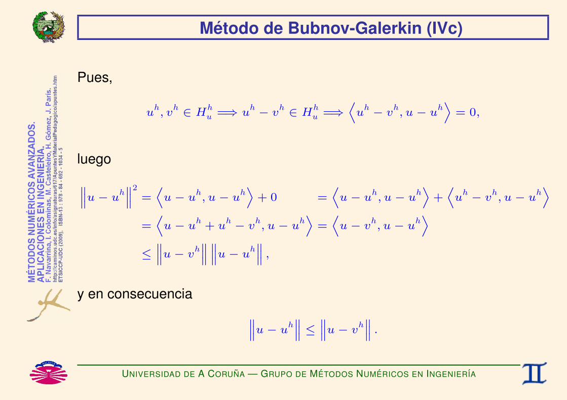
Metodo de Bubnov-Galerkin (IVc)
Pues,
uh, v
h ∈ Hhu =⇒ u
h − vh ∈ H
hu =⇒
Du
h − vh, u− u
hE
= 0,
luego
‚‚‚u− uh‚‚‚2
=D
u− uh, u− u
hE
+ 0 =D
u− uh, u− u
hE
+D
uh − v
h, u− u
hE
=D
u− uh+ u
h − vh, u− u
hE
=D
u− vh, u− u
hE
≤‚‚‚u− v
h‚‚‚ ‚‚‚u− u
h‚‚‚ ,
y en consecuencia ‚‚‚u− uh‚‚‚ ≤ ‚‚‚u− v
h‚‚‚ .
UNIVERSIDAD DE A CORUNA — GRUPO DE METODOS NUMERICOS EN INGENIERIA
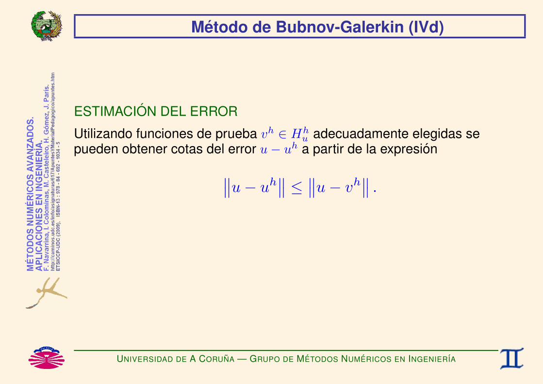
Metodo de Bubnov-Galerkin (IVd)
ESTIMACION DEL ERROR
Utilizando funciones de prueba vh ∈ Hhu adecuadamente elegidas se
pueden obtener cotas del error u− uh a partir de la expresion∥∥u− uh∥∥ ≤ ∥∥u− vh
∥∥ .
UNIVERSIDAD DE A CORUNA — GRUPO DE METODOS NUMERICOS EN INGENIERIA

Eleccion de las Funciones de Prueba (Ia)
Algunas posibilidades. . .
1) SOPORTE GLOBAL → METODO DE RITZ
♣ Ejemplos:B a) φi(x) = xi, i=1,...,ν →Hh
u = Pν(x).B b) Series de FourierB c) . . .
♠ Ke es LLENA→ tiempo de computacion T (ν3).
♠ Ke puede ser MAL-CONDICIONADA. (*)
(*) EL numero de condicion depende de la base de funciones de prueba que se hayan elegido.
UNIVERSIDAD DE A CORUNA — GRUPO DE METODOS NUMERICOS EN INGENIERIA

Eleccion de las Funciones de Prueba (Ib)
2) SOPORTE LOCAL → METODO DE ELEMENTOS FINITOS
♣ Ejemplos:B a) Funciones en escalon.B b) Poligonales a trozos.B c) Splines en general.
♥ Se pretende que Ke sea SPARSE.
♥ Se pretende que Ke sea BIEN-CONDICIONADA.
UNIVERSIDAD DE A CORUNA — GRUPO DE METODOS NUMERICOS EN INGENIERIA

Mınimos Cuadrados (I)
MINIMOS CUADRADOS (Least Squares)
Hallar u(x), x ∈ [a, b],
que MINIMIZA Q[u(x)] =∫ b
a
r(x)p(x)r(x) dx, (*)
siendo r(x) = f(x)− u(x),
(*) La funcion de peso p(x) debe verificar p(x) > 0 ∀x ∈ [a, b].
UNIVERSIDAD DE A CORUNA — GRUPO DE METODOS NUMERICOS EN INGENIERIA

Mınimos Cuadrados (IIa)
FUNCIONES DE PRUEBA (Trial Functions)
Sea la base de funciones de prueba φi(x)i=0,...,ν.
Dada la aproximacion inicial u0(x), buscamos una mejor aproximacion
u(x) ≈ uh(x) = u0(x) +ν∑
i=0
αiφi(x), uh(x) ∈ Hhu ⊂ Hu,
u(x) ≈ uh(x) = u0(x) + ΦT (x) α, con Φ(x) =
φ0(x)
...φν(x)
, α =
α0...αν
.
El residuo correspondiente a la aproximacion uh(x) sera
rh(x) = f(x)− uh(x) = r0(x)−ν∑
i=0
αiφi(x), con r0(x) = f(x)− u0(x)
rh(x) = f(x)− uh(x) = r0(x)− ΦT (x) α, con r0(x) = f(x)− u0(x).
UNIVERSIDAD DE A CORUNA — GRUPO DE METODOS NUMERICOS EN INGENIERIA
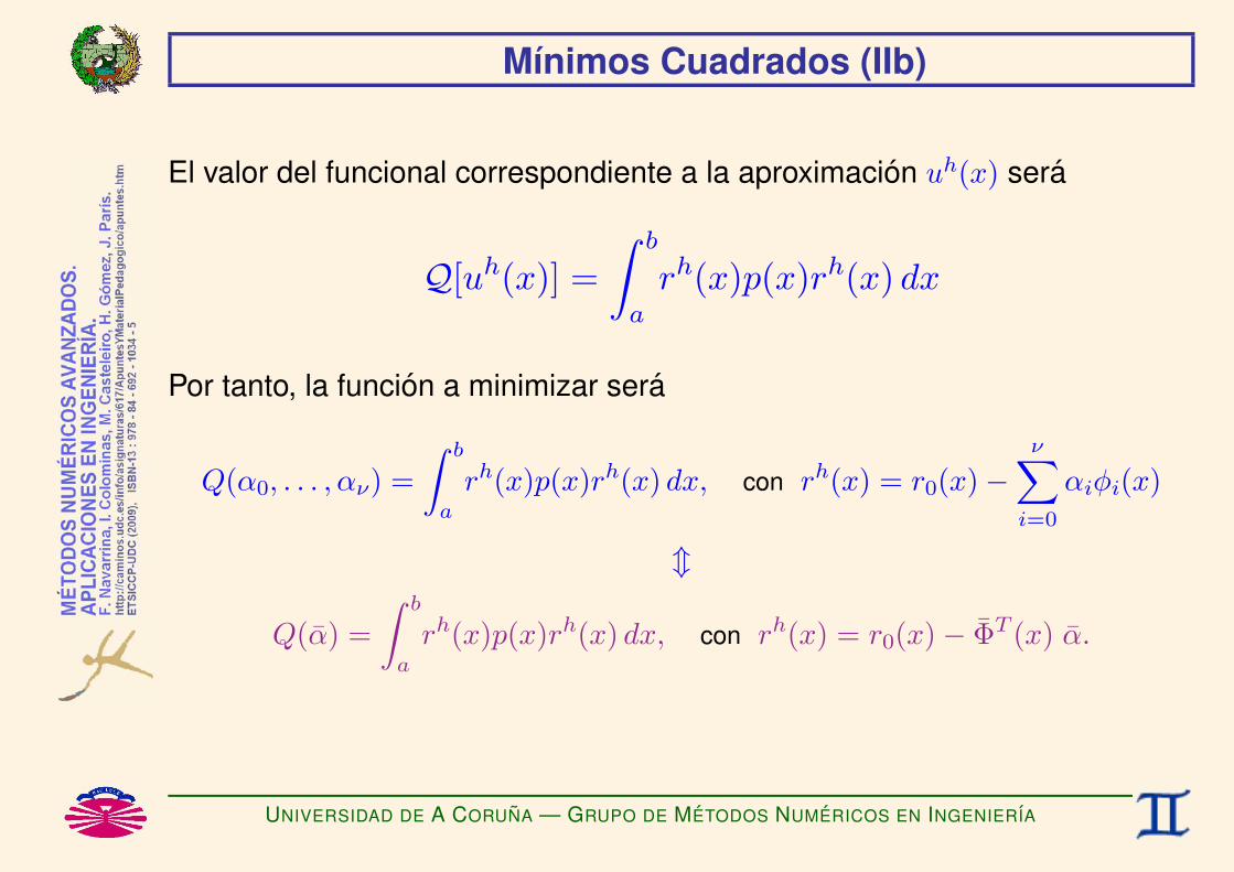
Mınimos Cuadrados (IIb)
El valor del funcional correspondiente a la aproximacion uh(x) sera
Q[uh(x)] =∫ b
a
rh(x)p(x)rh(x) dx
Por tanto, la funcion a minimizar sera
Q(α0, . . . , αν) =∫ b
a
rh(x)p(x)rh(x) dx, con rh(x) = r0(x)−ν∑
i=0
αiφi(x)
m
Q(α) =∫ b
a
rh(x)p(x)rh(x) dx, con rh(x) = r0(x)− ΦT (x) α.
UNIVERSIDAD DE A CORUNA — GRUPO DE METODOS NUMERICOS EN INGENIERIA
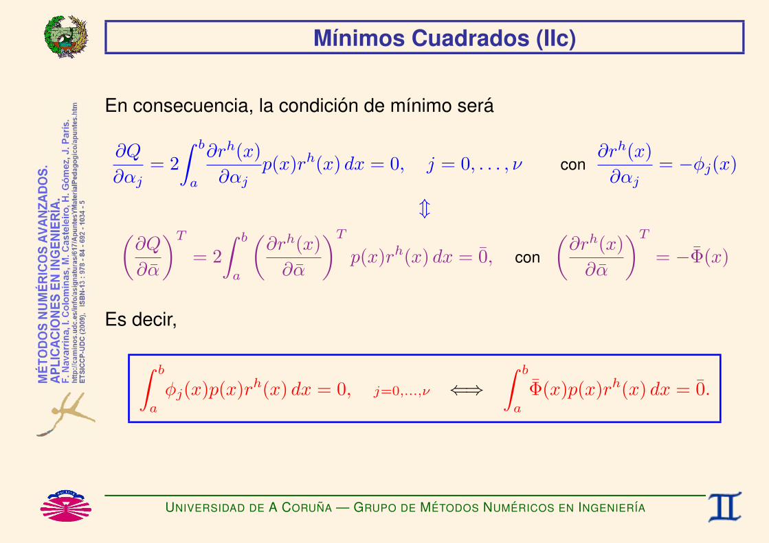
Mınimos Cuadrados (IIc)
En consecuencia, la condicion de mınimo sera
∂Q
∂αj= 2∫ b
a
∂rh(x)∂αj
p(x)rh(x) dx = 0, j = 0, . . . , ν con∂rh(x)∂αj
= −φj(x)
m(∂Q
∂α
)T
= 2∫ b
a
(∂rh(x)
∂α
)T
p(x)rh(x) dx = 0, con
(∂rh(x)
∂α
)T
= −Φ(x)
Es decir,
∫ b
a
φj(x)p(x)rh(x) dx = 0, j=0,...,ν ⇐⇒∫ b
a
Φ(x)p(x)rh(x) dx = 0.
UNIVERSIDAD DE A CORUNA — GRUPO DE METODOS NUMERICOS EN INGENIERIA

Mınimos Cuadrados (IIIa)
Luego, la formulacion de MINIMOS CUADRADOS equivale a plantear elMETODO DE RESIDUOS PONDERADOS con las funciones de test
ωj(x) = φj(x)p(x), j=0,...,ν,
Ω(x) = Φ(x)p(x).
Por tanto se obtiene
Ke =ˆkji˜i=0,...,νj=0,...,ν
, kji =
Z b
aφj(x)p(x)φi(x) dx ⇐⇒ Ke =
Z b
aΦ(x)p(x)ΦT (x) dx
f =˘
fj¯
j=0,...,ν, fj =
Z b
aφj(x)p(x)r0(x) dx ⇐⇒ f =
Z b
aΦ(x)p(x)r0(x) dx.
UNIVERSIDAD DE A CORUNA — GRUPO DE METODOS NUMERICOS EN INGENIERIA

Mınimos Cuadrados (IIIb)
Esto es2666666664
Z b
a
φ0(x)p(x)φ0(x) dx
Z b
a
φ0(x)p(x)φ1(x) dx . . .
Z b
a
φ0(x)p(x)φν(x) dxZ b
a
φ1(x)p(x)φ0(x) dx
Z b
a
φ1(x)p(x)φ1(x) dx . . .
Z b
a
φ1(x)p(x)φν(x) dx
... ... ...Z b
a
φν(x)p(x)φ0(x) dx
Z b
a
φν(x)p(x)φ1(x) dx . . .
Z b
a
φν(x)p(x)φν(x) dx
37777777758><>:
α0
α1...αν
9>=>; =
=
8>>>>>>>><>>>>>>>>:
Z b
a
φ0(x)p(x) [f(x)− u0(x)] dxZ b
a
φ1(x)p(x) [f(x)− u0(x)] dx
...Z b
a
φν(x)p(x) [f(x)− u0(x)] dx
9>>>>>>>>=>>>>>>>>;. (*)
(*) Cuando la funcion de peso p(x) es constante, MINIMOS CUADRADOS equivale al METODO DE BUBNOV-GALERKIN.
UNIVERSIDAD DE A CORUNA — GRUPO DE METODOS NUMERICOS EN INGENIERIA

Notacion en Formas Bilineales (I)
RESIDUOS PONDERADOS (Weighted Residuals)
Hallar u(x) ∈ Hu,
que VERIFICA a(ω, u) = (ω, f) ∀ω(x) ∈ Hω,
siendo a(ω, u) =∫ b
a
ω(x)u(x) dx,
(ω, f) =∫ b
a
ω(x)f(x) dx.
UNIVERSIDAD DE A CORUNA — GRUPO DE METODOS NUMERICOS EN INGENIERIA

Notacion en Formas Bilineales (IIa)
FUNCIONES DE PRUEBA (Trial Functions)
Sea la base de funciones de prueba φi(x)i=0,...,ν.
Dada la aproximacion inicial u0(x), buscamos una mejor aproximacion
u(x) ≈ uh(x) = u0(x) +ν∑
i=0
αiφi(x), uh(x) ∈ Hhu ⊂ Hu,
u(x) ≈ uh(x) = u0(x) + ΦT (x) α, con Φ(x) =
φ0(x)
...φν(x)
, α =
α0...αν
.
El residuo correspondiente a la aproximacion u0(x) sera
r0(x) = f(x)− u0(x)
UNIVERSIDAD DE A CORUNA — GRUPO DE METODOS NUMERICOS EN INGENIERIA

Notacion en Formas Bilineales (IIb)
En general no sera posible que uh(x) = u(x) ∀x ∈ [a, b] (*), por lo que
uh(x) 6= u(x) =⇒ no es posible que a(ω, uh) = (ω, f) ∀ω(x) ∈ Hω.
(*) Salvo que u(x)− u0(x) este contenido en el subespacio generado por las funciones de prueba.
UNIVERSIDAD DE A CORUNA — GRUPO DE METODOS NUMERICOS EN INGENIERIA

Notacion en Formas Bilineales (IIIa)
FUNCIONES DE TEST (Test Functions)
Sea la base de funciones de test ωj(x)j=0,...,ν.
Sea
ωh(x) =ν∑
j=0
βjωj(x), ωh(x) ∈ Hhω ⊂ Hω,
ωh(x) = ΩT (x) β = βT Ω(x), con Ω(x) =
ω0(x)
...ων(x)
, β =
β0...βν
.
Nos proponemos obtener la aproximacion uh(x) ∈ Hhu que verifique
a(ωh, uh) = (ωh, f) ∀ωh(x) ∈ Hhω.
UNIVERSIDAD DE A CORUNA — GRUPO DE METODOS NUMERICOS EN INGENIERIA

Notacion en Formas Bilineales (IIIb)
Pero
a(ωh, u
h) = (ω
h, f) ∀ω
h(x) ∈ H
hω
m
a(
νXj=0
βjωj, uh) = (
νXj=0
βjωj, f) ∀ βj ⇐⇒ a(βT
Ω, uh) = (β
TΩ, f) ∀β
mνX
j=0
βj
„a(ωj, u
h)− (ωj, f)
«= 0 ∀ βj ⇐⇒ β
T
„a(Ω, u
h)− (Ω, f)
«= 0 ∀β
m
a(ωj, uh) = (ωj, f) j=0,...,ν ⇐⇒ a(Ω, u
h) = (Ω, f).
UNIVERSIDAD DE A CORUNA — GRUPO DE METODOS NUMERICOS EN INGENIERIA

Notacion en Formas Bilineales (IVa)
Por tanto,
a(ωj, u0 +
νXi=0
αiφi) = (ωj, f) ∀j ⇐⇒ a(Ω, u0 + ΦTα) = (Ω, f)
m
νXi=0
kjiz | a(ωj, φi) αi =
fjz | (ωj, r0) ∀j ⇐⇒
Kez | a(Ω, Φ
T) α =
fz | (Ω, r0)
m
νXi=0
kjiαi = fj j=0,...,ν ⇐⇒ Ke α = f .
UNIVERSIDAD DE A CORUNA — GRUPO DE METODOS NUMERICOS EN INGENIERIA
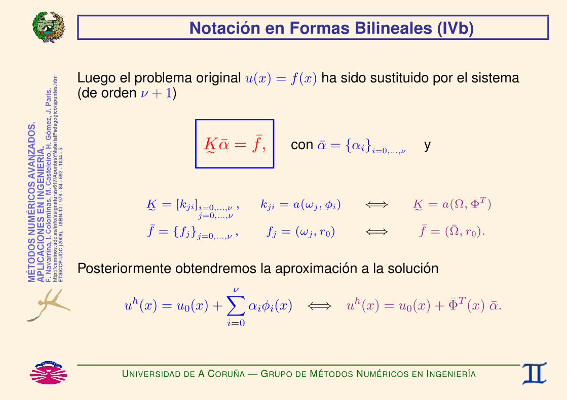
Notacion en Formas Bilineales (IVb)
Luego el problema original u(x) = f(x) ha sido sustituido por el sistema(de orden ν + 1)
K˜ α = f , con α = αii=0,...,νy
Ke = [kji]i=0,...,νj=0,...,ν
, kji = a(ωj, φi) ⇐⇒ Ke = a(Ω, ΦT )
f = fjj=0,...,ν , fj = (ωj, r0) ⇐⇒ f = (Ω, r0).
Posteriormente obtendremos la aproximacion a la solucion
uh(x) = u0(x) +ν∑
i=0
αiφi(x) ⇐⇒ uh(x) = u0(x) + ΦT (x) α.
UNIVERSIDAD DE A CORUNA — GRUPO DE METODOS NUMERICOS EN INGENIERIA


INTRODUCCION AL METODO DE ELEMENTOS FINITOS:APROXIMACION DE FUNCIONES
F. Navarrina, I. Colominas, M. Casteleiro, H. Gomez, J. Parıs
GMNI — GRUPO DE METODOS NUMERICOS EN INGENIERIA
Departamento de Metodos Matematicos y de RepresentacionEscuela Tecnica Superior de Ingenieros de Caminos, Canales y Puertos
Universidad de A Coruna, Espana
e-mail: [email protected] web: http://caminos.udc.es/gmni
UNIVERSIDAD DE A CORUNA — GRUPO DE METODOS NUMERICOS EN INGENIERIA

INDICE
I Forma Debil
I Metodo de Elementos Finitos
UNIVERSIDAD DE A CORUNA — GRUPO DE METODOS NUMERICOS EN INGENIERIA

Forma Debil (I)
FORMA DEBIL (Residuos Ponderados)
Hallar u(x) ∈ Hu,
que VERIFICA a(ω, u) = (ω, f) ∀ω(x) ∈ Hω,
siendo a(ω, u) =∫ b
a
ω(x)u(x) dx,
(ω, f) =∫ b
a
ω(x)f(x) dx.
UNIVERSIDAD DE A CORUNA — GRUPO DE METODOS NUMERICOS EN INGENIERIA
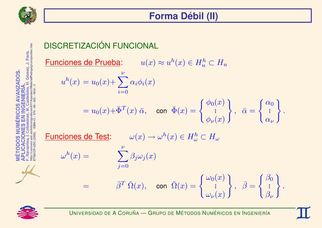
Forma Debil (II)
DISCRETIZACION FUNCIONAL
Funciones de Prueba: u(x) ≈ uh(x) ∈ Hhu ⊂ Hu
uh(x) = u0(x)+ν∑
i=0
αiφi(x)
= u0(x)+ΦT (x) α, con Φ(x) =
φ0(x)
...φν(x)
, α =
α0...αν
.
Funciones de Test: ω(x) → ωh(x) ∈ Hhω ⊂ Hω
ωh(x) =ν∑
j=0
βjωj(x)
= βT Ω(x), con Ω(x) =
ω0(x)
...ων(x)
, β =
β0...βν
.
UNIVERSIDAD DE A CORUNA — GRUPO DE METODOS NUMERICOS EN INGENIERIA
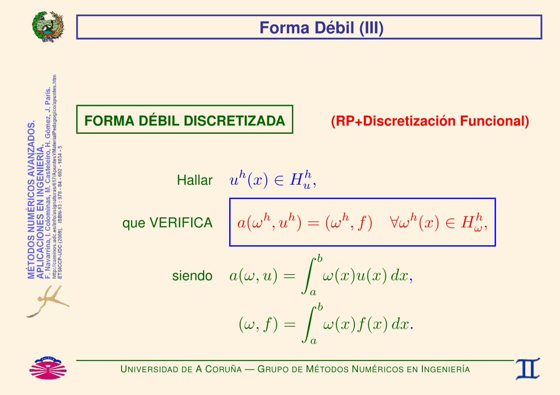
Forma Debil (III)
FORMA DEBIL DISCRETIZADA (RP+Discretizacion Funcional)
Hallar uh(x) ∈ Hhu ,
que VERIFICA a(ωh, uh) = (ωh, f) ∀ωh(x) ∈ Hhω,
siendo a(ω, u) =∫ b
a
ω(x)u(x) dx,
(ω, f) =∫ b
a
ω(x)f(x) dx.
UNIVERSIDAD DE A CORUNA — GRUPO DE METODOS NUMERICOS EN INGENIERIA

Forma Debil (IV)
REDUCCION A UN SISTEMA ALGEBRAICO
El problema u(x) = f(x) se reduce al sistema algebraico (de orden ν + 1)
K˜ α = f , con α = αii=0,...,νy
K˜ = [kji]i=0,...,νj=0,...,ν
, kji = a(ωj, φi) ⇐⇒ K˜ = a(Ω, ΦT )
f = fjj=0,...,ν, fj = (ωj, f − u0) ⇐⇒ f = (Ω, f − u0).
UNIVERSIDAD DE A CORUNA — GRUPO DE METODOS NUMERICOS EN INGENIERIA

Metodo de Elementos Finitos (I)
DISCRETIZACION DEL DOMINIO DE INTEGRACION
Diremos que el dominio [a, b] se ha discretizado en unaMALLA DE ELEMENTOS FINITOS si
[a, b] =N⋃
e=1
Ee,
Ee ∩
Ef= ∅ ∀e 6= f,
donde Ee es el ELEMENTO FINITO numero e.
Ejemplo:
Ee = [xe−1, xe], con a = x0 < x1 < . . . < xN = b.
UNIVERSIDAD DE A CORUNA — GRUPO DE METODOS NUMERICOS EN INGENIERIA

Metodo de Elementos Finitos (II)
Efecto: INTEGRACION ELEMENTO A ELEMENTO
∫ b
a
g(x) dx =N∑
e=1
∫Ee
g(x) dx.
UNIVERSIDAD DE A CORUNA — GRUPO DE METODOS NUMERICOS EN INGENIERIA
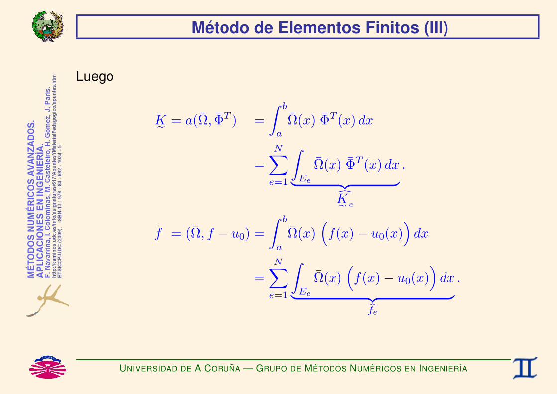
Metodo de Elementos Finitos (III)
Luego
K˜ = a(Ω, ΦT ) =∫ b
a
Ω(x) ΦT (x) dx
=N∑
e=1
∫Ee
Ω(x) ΦT (x) dx︸ ︷︷ ︸dK˜ e
.
f = (Ω, f − u0) =∫ b
a
Ω(x)(f(x)− u0(x)
)dx
=N∑
e=1
∫Ee
Ω(x)(f(x)− u0(x)
)dx︸ ︷︷ ︸bfe
.
UNIVERSIDAD DE A CORUNA — GRUPO DE METODOS NUMERICOS EN INGENIERIA


METODO DE RESIDUOS PONDERADOS:PROBLEMAS DE EQUILIBRIO 1D
F. Navarrina, I. Colominas, M. Casteleiro, H. Gomez, J. Parıs
GMNI — GRUPO DE METODOS NUMERICOS EN INGENIERIA
Departamento de Metodos Matematicos y de RepresentacionEscuela Tecnica Superior de Ingenieros de Caminos, Canales y Puertos
Universidad de A Coruna, Espana
e-mail: [email protected] web: http://caminos.udc.es/gmni
UNIVERSIDAD DE A CORUNA — GRUPO DE METODOS NUMERICOS EN INGENIERIA

INDICE
I Problema Conceptual
I Planteamientos Alternativos
I Residuos Ponderados: Forma Debil
I Residuos Ponderados: Aproximacion Numerica
I Residuos Ponderados: Error de Aproximacion
I Eleccion de las Funciones de Test
I Metodo de Bubnov-Galerkin
I Eleccion de las Funciones de Prueba
I Notacion en Formas Bilineales
UNIVERSIDAD DE A CORUNA — GRUPO DE METODOS NUMERICOS EN INGENIERIA

Problema Conceptual (I)
Sea el problema de equilibrio 1D:
UNIVERSIDAD DE A CORUNA — GRUPO DE METODOS NUMERICOS EN INGENIERIA
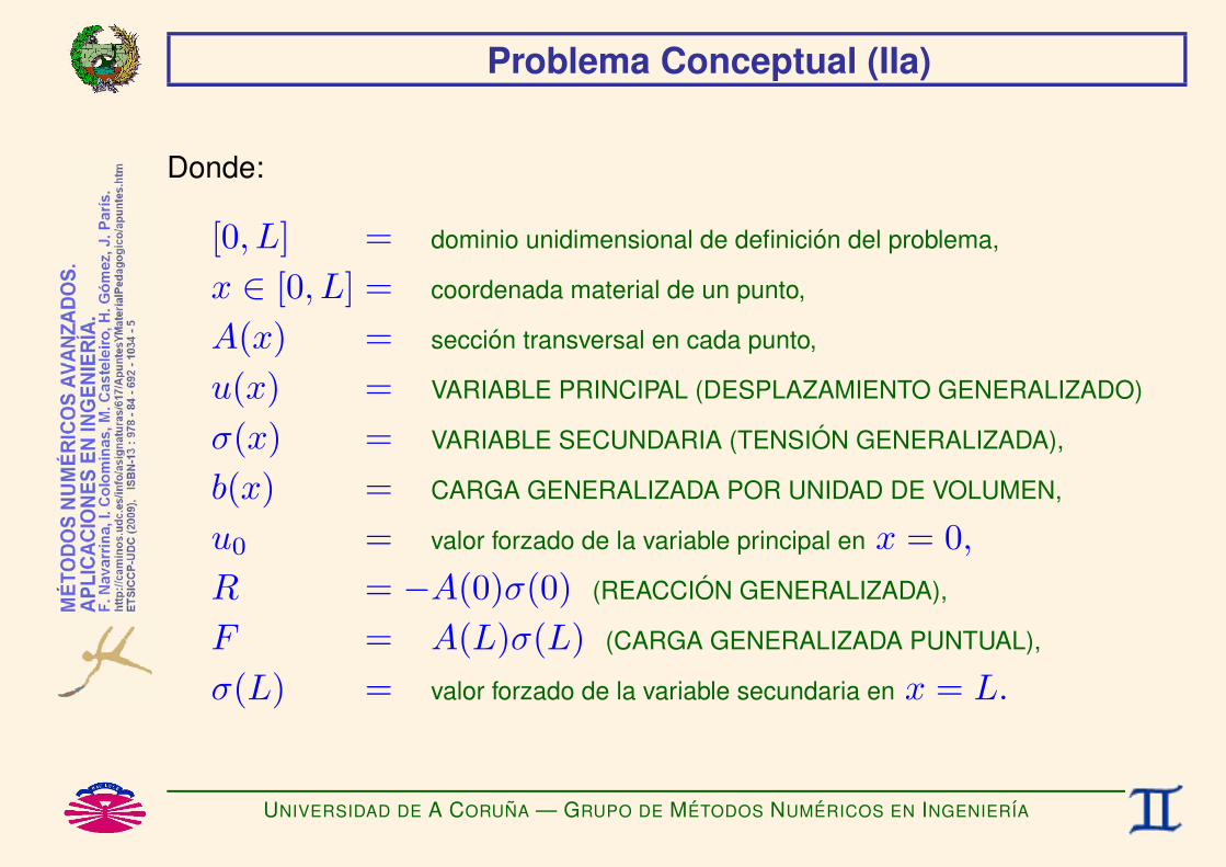
Problema Conceptual (IIa)
Donde:
[0, L] = dominio unidimensional de definicion del problema,
x ∈ [0, L] = coordenada material de un punto,
A(x) = seccion transversal en cada punto,
u(x) = VARIABLE PRINCIPAL (DESPLAZAMIENTO GENERALIZADO)
σ(x) = VARIABLE SECUNDARIA (TENSION GENERALIZADA),
b(x) = CARGA GENERALIZADA POR UNIDAD DE VOLUMEN,
u0 = valor forzado de la variable principal en x = 0,R = −A(0)σ(0) (REACCION GENERALIZADA),
F = A(L)σ(L) (CARGA GENERALIZADA PUNTUAL),
σ(L) = valor forzado de la variable secundaria en x = L.
UNIVERSIDAD DE A CORUNA — GRUPO DE METODOS NUMERICOS EN INGENIERIA

Problema Conceptual (IIb)
La relacion entre la variable principal u(x) y la variable secundaria u(x) seestablece a traves de una variable intermedia ε(x) (DEFORMACIONGENERALIZADA), de forma que tendremos dos tipos de ecuaciones:
I ECUACIONES DE COMPATIBILIDAD(o relaciones deformacion—desplazamiento):
u(x) −→ ε(x).
I ECUACIONES CONSTITUTIVAS(o relaciones tension—deformacion):
ε(x) −→ σ(x).
UNIVERSIDAD DE A CORUNA — GRUPO DE METODOS NUMERICOS EN INGENIERIA

Problema Conceptual (III)
Modelo Matematico Lineal:
Dados A(x), b(x), E(x), u0, F,
Hallar u(x), σ(x), x ∈ [0, L], que verifican
∂
∂x(Aσ) +Ab = 0 ∀x ∈ (0, L), (ECUACION DE EQUILIBRIO)
σ = Eε, (ECUACION CONSTITUTIVA)
ε =∂u
∂x, (ECUACION DE COMPATIBILIDAD)
−A(L)σ(L) + F = 0, (C.C. NATURAL)
u(0) = u0. (C.C. ESENCIAL)
El problema anterior puede representar diferentes fenomenos fısicos,como. . .
UNIVERSIDAD DE A CORUNA — GRUPO DE METODOS NUMERICOS EN INGENIERIA

Problema Conceptual (IVa)
Barra elastica a traccion–compresion
[0, L] = barra de longitud L.
x ∈ [0, L] = coordenada material de un punto.
A(x) = seccion transversal.
u(x) = DESPLAZAMIENTO.
ε(x) = DEFORMACION.
σ(x) = TENSION.
b(x) = FUERZA EXTERIOR POR UNIDAD DE VOLUMEN.
u0 = DESPLAZAMIENTO PREFIJADO EN x = 0.R = −A(0)σ(0) (REACCION),
F = A(L)σ(L) (FUERZA PUNTUAL EXTERIOR),
E = MODULO DE ELASTICIDAD.
En este caso, la ecuacion constitutiva se denomina LEY DE HOOKE.UNIVERSIDAD DE A CORUNA — GRUPO DE METODOS NUMERICOS EN INGENIERIA

Problema Conceptual (IVb)
Difusion de contaminante en un canal
[0, L] = canal de longitud L.
x ∈ [0, L] = coordenada material de un punto.
A(x) = seccion transversal.
u(x) = CONCENTRACION DE CONTAMINANTE.
ε(x) = GRADIENTE DE CONCENTRACION DE CONTAMINANTE.
σ(x) = DENSIDAD DE FLUJO DE CONTAMINANTE.
b(x) = SUMIDERO DE CONTAMINANTE POR UNIDAD DE VOLUMEN.
u0 = CONCENTRACION PREFIJADA EN x = 0.R = −A(0)σ(0) (REACCION),
F = A(L)σ(L) (FLUJO DE CONTAMINANTE FORZADO),
E = −γ, γ = DIFUSIVIDAD.
En este caso, la ecuacion constitutiva se denomina LEY DE FICKS.UNIVERSIDAD DE A CORUNA — GRUPO DE METODOS NUMERICOS EN INGENIERIA

Problema Conceptual (IVc)
Difusion de calor en una barra
[0, L] = barra de longitud L.
x ∈ [0, L] = coordenada material de un punto.
A(x) = seccion transversal.
u(x) = TEMPERATURA.
ε(x) = GRADIENTE DE TEMPERATURA.
σ(x) = DENSIDAD DE FLUJO DE CALOR.
b(x) = SUMIDERO DE CALOR POR UNIDAD DE VOLUMEN.
u0 = TEMPERATURA PREFIJADA EN x = 0.R = −A(0)σ(0) (REACCION),
F = A(L)σ(L) (FLUJO DE CALOR FORZADO),
E = −γ, γ = CONDUCTIVIDAD TERMICA.
En este caso, la ecuacion constitutiva se denomina LEY DE FOURIER.UNIVERSIDAD DE A CORUNA — GRUPO DE METODOS NUMERICOS EN INGENIERIA

Problema Conceptual (IVd)
Corriente electrica en un conductor
[0, L] = conductor de longitud L.
x ∈ [0, L] = coordenada material de un punto.
A(x) = seccion transversal.
u(x) = POTENCIAL ELECTRICO.
ε(x) = GRADIENTE DE POTENCIAL.
σ(x) = DENSIDAD DE CORRIENTE.
b(x) = SUMIDERO DE CORRIENTE POR UNIDAD DE VOLUMEN.
u0 = POTENCIAL PREFIJADO EN x = 0.R = −A(0)σ(0) (REACCION),
F = A(L)σ(L) (INTENSIDAD DE CORRIENTE FORZADA),
E = −γ, γ = CONDUCTIVIDAD ELECTRICA.
En este caso, la ecuacion constitutiva se denomina LEY DE OHM.UNIVERSIDAD DE A CORUNA — GRUPO DE METODOS NUMERICOS EN INGENIERIA

Planteamientos Alternativos (I)
a) FORMA ORIGINAL
Hallar u(x), x ∈ [0, L],
que VERIFICA r(x) = 0 ∀x ∈ (0, L), rΓ = 0, (*)
siendo
r(x) =∂
∂x(Aσ) +Ab, (ECUACION DE EQUILIBRIO)
σ = Eε, (ECUACION CONSTITUTIVA)
ε =∂u
∂x, (ECUACION DE COMPATIBILIDAD)
rΓ = −A(L)σ(L) + F, (C.C. NATURAL)
u(0) = u0. (C.C. ESENCIAL)
(*) FORMA FUERTE o STRONG FORM.
UNIVERSIDAD DE A CORUNA — GRUPO DE METODOS NUMERICOS EN INGENIERIA

Planteamientos Alternativos (IIa)
b) RESIDUOS PONDERADOS
Hallar u(x), x ∈ [0, L],
que VERIFICA∫ L
0
ω(x)r(x) dx+ ωΓrΓ = 0 ∀ω(x), ωΓ (*)
siendo
r(x) =∂
∂x(Aσ) +Ab, (ECUACION DE EQUILIBRIO)
σ = Eε, (ECUACION CONSTITUTIVA)
ε =∂u
∂x, (ECUACION DE COMPATIBILIDAD)
rΓ = −A(L)σ(L) + F, (C.C. NATURAL)
u(0) = u0. (C.C. ESENCIAL)
(*) FORMA DEBIL o WEAK FORM.
UNIVERSIDAD DE A CORUNA — GRUPO DE METODOS NUMERICOS EN INGENIERIA
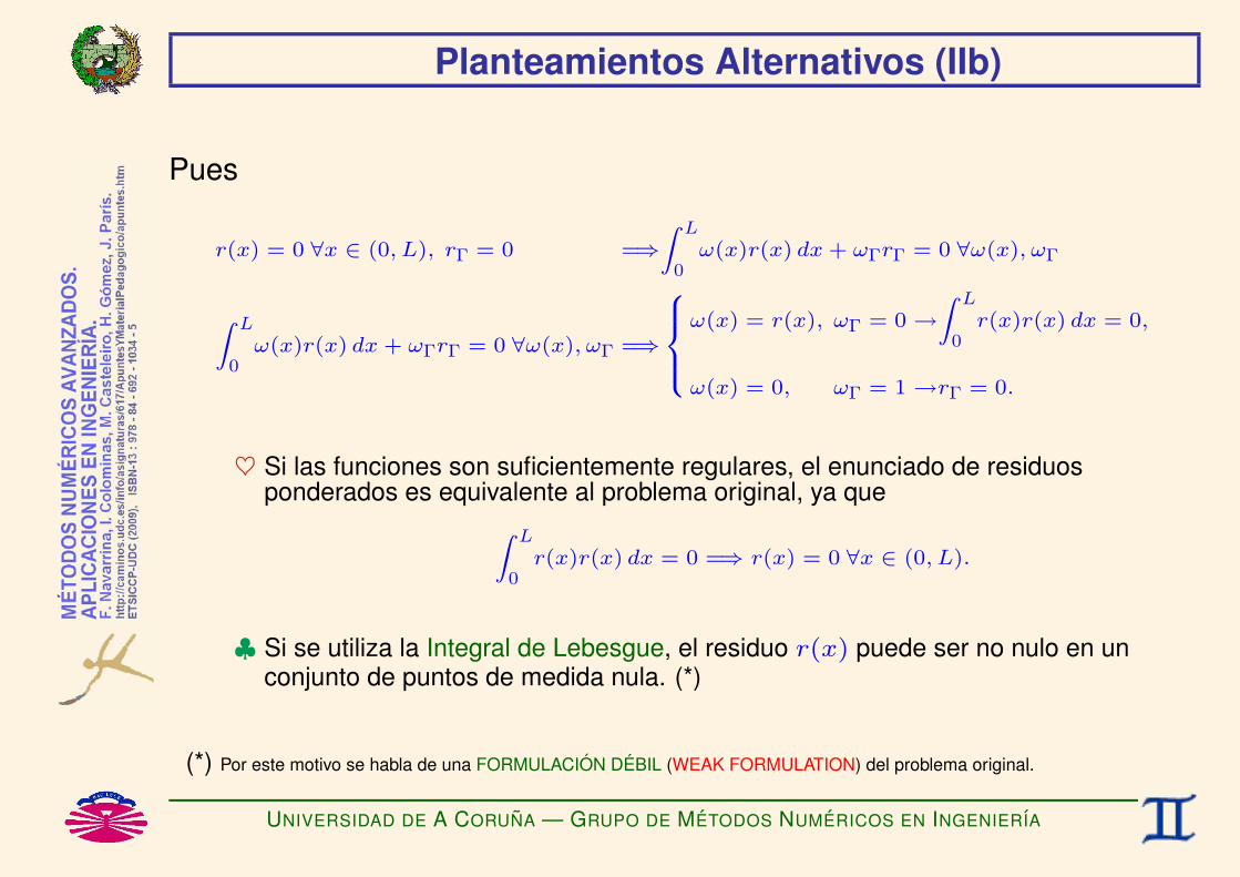
Planteamientos Alternativos (IIb)
Pues
r(x) = 0 ∀x ∈ (0, L), rΓ = 0 =⇒Z L
0ω(x)r(x) dx+ ωΓrΓ = 0 ∀ω(x), ωΓ
Z L
0ω(x)r(x) dx+ ωΓrΓ = 0 ∀ω(x), ωΓ =⇒
8>><>>:ω(x) = r(x), ωΓ = 0 →
Z L
0r(x)r(x) dx = 0,
ω(x) = 0, ωΓ = 1 →rΓ = 0.
♥ Si las funciones son suficientemente regulares, el enunciado de residuosponderados es equivalente al problema original, ya queZ L
0r(x)r(x) dx = 0 =⇒ r(x) = 0 ∀x ∈ (0, L).
♣ Si se utiliza la Integral de Lebesgue, el residuo r(x) puede ser no nulo en unconjunto de puntos de medida nula. (*)
(*) Por este motivo se habla de una FORMULACION DEBIL (WEAK FORMULATION) del problema original.
UNIVERSIDAD DE A CORUNA — GRUPO DE METODOS NUMERICOS EN INGENIERIA

Planteamientos Alternativos (IIc)
Sin perdida de generalidad podemos elegir
ωΓ = ω(L),
pues
r(x) = 0 ∀x ∈ (0, L), rΓ = 0 =⇒Z L
0ω(x)r(x) dx+ ω(L)rΓ = 0 ∀ω(x)
Z L
0ω(x)r(x) dx+ ω(L)rΓ = 0 ∀ω(x) =⇒
8<:ω(x) = r(x) ∗ (L− x) →r(x) = 0∀x ∈ (0, L), (∗)
r(x) = 0∀x ∈ (0, L), ω(L) 6= 0 →rΓ = 0.
(*) Pues si las funciones son suficientemente regulares,
Z L
0r(x)r(x)
≥0z | (L− x) dx = 0 =⇒ r(x) = 0∀x ∈ (0, L).
UNIVERSIDAD DE A CORUNA — GRUPO DE METODOS NUMERICOS EN INGENIERIA

Planteamientos Alternativos (IId)
Por tanto, podemos adoptar el enunciado de residuos ponderados. . .
Hallar u(x), x ∈ [0, L],
que VERIFICA∫ L
0
ω(x)r(x) dx+ ω(L)rΓ = 0 ∀ω(x)
siendo
r(x) =∂
∂x(Aσ) +Ab, (ECUACION DE EQUILIBRIO)
σ = Eε, (ECUACION CONSTITUTIVA)
ε =∂u
∂x, (ECUACION DE COMPATIBILIDAD)
rΓ = −A(L)σ(L) + F, (C.C. NATURAL)
u(0) = u0. (C.C. ESENCIAL)
UNIVERSIDAD DE A CORUNA — GRUPO DE METODOS NUMERICOS EN INGENIERIA

Planteamientos Alternativos (IIIa)
c) MINIMOS CUADRADOS
Hallar u(x), x ∈ [0, L],
que MINIMIZA Q[u] =∫ L
0
r(x)p(x)r(x) dx+ rΓpΓrΓ, (*)
siendo
r(x) =∂
∂x(Aσ) +Ab, (ECUACION DE EQUILIBRIO)
σ = Eε, (ECUACION CONSTITUTIVA)
ε =∂u
∂x, (ECUACION DE COMPATIBILIDAD)
rΓ = −A(L)σ(L) + F, (C.C. NATURAL)
u(0) = u0. (C.C. ESENCIAL)
(*) La funcion de peso p(x) y el peso pΓ deben verificar p(x) > 0 ∀x ∈ [0, L], pΓ > 0.
UNIVERSIDAD DE A CORUNA — GRUPO DE METODOS NUMERICOS EN INGENIERIA

Planteamientos Alternativos (IIIb)
La condicion de mınimo equivale al PLANTEAMIENTO VARIACIONAL
Hallar u(x) x ∈ [0, L],
que VERIFICAdJ(λ)dλ
∣∣∣∣λ=0
= 0 ∀δu(x) tal que δu(0) = 0,
con J(λ) = Q[u+ λδu],
y por tantodJ(λ)dλ
∣∣∣∣λ=0
= 2∫ L
0
∂
∂x
(AE
∂δu
∂x
)p(x)r(x) dx
− 2(AE
∂δu
∂x
)∣∣∣∣x=L
pΓrΓ, (*)
UNIVERSIDAD DE A CORUNA — GRUPO DE METODOS NUMERICOS EN INGENIERIA
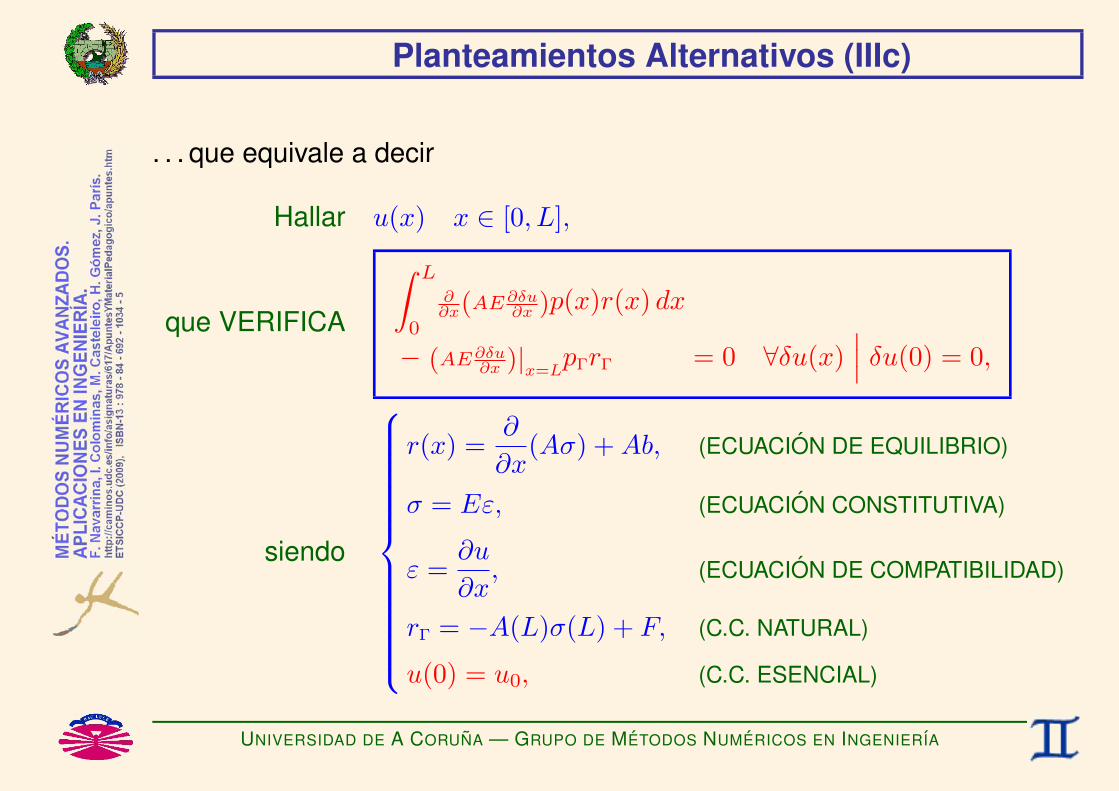
Planteamientos Alternativos (IIIc)
. . . que equivale a decir
Hallar u(x) x ∈ [0, L],
que VERIFICA
∫ L
0
∂∂x(AE∂δu∂x )p(x)r(x) dx
− (AE∂δu∂x )|x=LpΓrΓ = 0 ∀δu(x)∣∣∣ δu(0) = 0,
siendo
r(x) =∂
∂x(Aσ) +Ab, (ECUACION DE EQUILIBRIO)
σ = Eε, (ECUACION CONSTITUTIVA)
ε =∂u
∂x, (ECUACION DE COMPATIBILIDAD)
rΓ = −A(L)σ(L) + F, (C.C. NATURAL)
u(0) = u0, (C.C. ESENCIAL)
UNIVERSIDAD DE A CORUNA — GRUPO DE METODOS NUMERICOS EN INGENIERIA
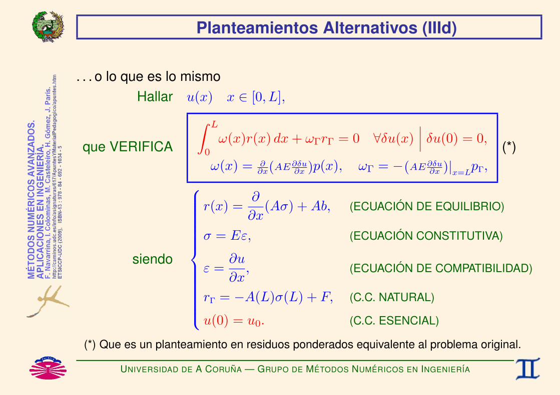
Planteamientos Alternativos (IIId)
. . . o lo que es lo mismoHallar u(x) x ∈ [0, L],
que VERIFICA
∫ L
0
ω(x)r(x) dx+ ωΓrΓ = 0 ∀δu(x)∣∣∣ δu(0) = 0,
ω(x) = ∂∂x(AE∂δu∂x )p(x), ωΓ = −(AE∂δu∂x )|x=LpΓ,
(*)
siendo
r(x) =∂
∂x(Aσ) +Ab, (ECUACION DE EQUILIBRIO)
σ = Eε, (ECUACION CONSTITUTIVA)
ε =∂u
∂x, (ECUACION DE COMPATIBILIDAD)
rΓ = −A(L)σ(L) + F, (C.C. NATURAL)
u(0) = u0. (C.C. ESENCIAL)
(*) Que es un planteamiento en residuos ponderados equivalente al problema original.
UNIVERSIDAD DE A CORUNA — GRUPO DE METODOS NUMERICOS EN INGENIERIA

Planteamientos Alternativos (IVa)
e) MINIMA ENERGIA
Hallar u(x), x ∈ [0, L],
que MINIMIZA
E [u] = +12
∫ L
0
ε(x)A(x)σ(x) dx
−∫ L
0
u(x)A(x)b(x) dx− u(L)F,
(*)
siendo
σ = Eε, (ECUACION CONSTITUTIVA)
ε =∂u
∂x, (ECUACION DE COMPATIBILIDAD)
u(0) = u0. (C.C. ESENCIAL)
(*) Si E < 0 se cambia el signo para que el funcional tenga un mınimo y no un maximo.
UNIVERSIDAD DE A CORUNA — GRUPO DE METODOS NUMERICOS EN INGENIERIA

Planteamientos Alternativos (IVb)
Se comprueba facilmente que la solucion del problema original u(x)minimiza la energıa, pues si v(x) = u(x) + δu(x) es cualquier otra funcionque tambien verifique la condicion de contorno esencial v(0) = u0, entoncesδu(0) = 0, y siendo
δε =∂δu
∂x, δσ = Eδε,
tenemos
E[u+ δu] = +1
2
Z L
0
(ε+ δε)A(σ + δσ) dx−Z L
0
(u+ δu)Ab dx−“u(L) + δu(L)
”F
= E[u] +1
2
Z L
0
(δεAσ + εAδσ + δεAδσ) dx−Z L
0
δuAb dx− δu(L)F
= E[u] +1
2
Z L
0
(δεAEε+ εAEδε+ δεAEδε) dx−Z L
0
δuAb dx− δu(L),
= E[u] +1
2
Z L
0
δεAEδε dx+
"Z L
0
δεAσ dx−Z L
0
δuAb dx− δu(L)F
#.
UNIVERSIDAD DE A CORUNA — GRUPO DE METODOS NUMERICOS EN INGENIERIA

Planteamientos Alternativos (IVc)
Integrando por partesZ L
0
δεAσ dx = +(δuAσ)˛L0−Z L
0
δu∂
∂x(Aσ) dx.
LuegoZ L
0
δεAσ dx−Z L
0
δuAb dx− δu(L)F =−Z L
0
δu
„∂
∂x(Aσ) + Ab
«| z
=0
dx
− δu(L) (−A(L)σ(L) + F )| z =0
= 0.
Por tanto,
E[u+ δu] = E[u] +1
2
≥0 ∀δεz | Z L
0
δεAEδε dx
≥ E[u] ∀δu˛δu(0) = 0.
UNIVERSIDAD DE A CORUNA — GRUPO DE METODOS NUMERICOS EN INGENIERIA

Planteamientos Alternativos (IVd)
La condicion de mınimo equivale al PLANTEAMIENTO VARIACIONAL
Hallar u(x), x ∈ [0, L],
que VERIFICAdJ(λ)dλ
∣∣∣∣λ=0
= 0 ∀δu(x) tal que δu(0) = 0,
con J(λ) = E [u+ λδu],
y por tantodJ(λ)dλ
∣∣∣∣λ=0
= +∫ L
0
∂δu
∂xA(x)E(x)
∂u
∂xdx
−∫ L
0
δu(x)A(x)b(x) dx− δu(L)F,
UNIVERSIDAD DE A CORUNA — GRUPO DE METODOS NUMERICOS EN INGENIERIA

Planteamientos Alternativos (IVe)
. . . que conduce al PRINCIPIO DE LOS TRABAJOS VIRTUALES (PTV)
Hallar u(x), x ∈ [0, L],
que VERIFICA
+∫ L
0
∂δu
∂xA(x)σ(x) dx
−∫ L
0
δu(x)A(x)b(x) dx
− δu(L)F = 0 ∀δu(x)∣∣∣ δu(0) = 0,
siendo
σ = Eε, (ECUACION CONSTITUTIVA)
ε =∂u
∂x, (ECUACION DE COMPATIBILIDAD)
u(0) = u0. (C.C. ESENCIAL)
UNIVERSIDAD DE A CORUNA — GRUPO DE METODOS NUMERICOS EN INGENIERIA

Planteamientos Alternativos (IVf)
Integrando por partes se obtiene,
Hallar u(x), x ∈ [0, L],
que VERIFICA
+(δu(x)A(x)σ(x)
)∣∣∣L0
−∫ L
0
δu(x)(∂
∂x(Aσ) +A(x)b(x)
)dx
− δu(L)F = 0 ∀δu(x)∣∣∣ δu(0) = 0,
siendo
σ = Eε, (ECUACION CONSTITUTIVA)
ε =∂u
∂x, (ECUACION DE COMPATIBILIDAD)
u(0) = u0, (C.C. ESENCIAL)
UNIVERSIDAD DE A CORUNA — GRUPO DE METODOS NUMERICOS EN INGENIERIA

Planteamientos Alternativos (IVg)
. . . o lo que es lo mismo,
Hallar u(x), x ∈ [0, L],
que VERIFICA
∫ L
0
ω(x)r(x) dx+ ωΓrΓ = 0 ∀δu(x)∣∣∣ δu(0) = 0,
ω(x) = δu(x), ωΓ = δu(L),(*)
siendo
r(x) =∂
∂x(Aσ) +Ab, (ECUACION DE EQUILIBRIO)
σ = Eε, (ECUACION CONSTITUTIVA)
ε =∂u
∂x, (ECUACION DE COMPATIBILIDAD)
rΓ = −A(L)σ(L) + F, (C.C. NATURAL)
u(0) = u0. (C.C. ESENCIAL)
(*) Que es un planteamiento en residuos ponderados equivalente al problema original.
UNIVERSIDAD DE A CORUNA — GRUPO DE METODOS NUMERICOS EN INGENIERIA

Residuos Ponderados: Forma Debil (I)
PLAN DE TRABAJO
UNIVERSIDAD DE A CORUNA — GRUPO DE METODOS NUMERICOS EN INGENIERIA
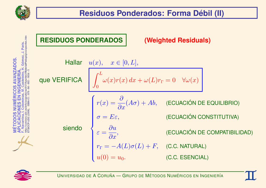
Residuos Ponderados: Forma Debil (II)
RESIDUOS PONDERADOS (Weighted Residuals)
Hallar u(x), x ∈ [0, L],
que VERIFICA∫ L
0
ω(x)r(x) dx+ ω(L)rΓ = 0 ∀ω(x)
siendo
r(x) =∂
∂x(Aσ) +Ab, (ECUACION DE EQUILIBRIO)
σ = Eε, (ECUACION CONSTITUTIVA)
ε =∂u
∂x, (ECUACION DE COMPATIBILIDAD)
rΓ = −A(L)σ(L) + F, (C.C. NATURAL)
u(0) = u0. (C.C. ESENCIAL)
UNIVERSIDAD DE A CORUNA — GRUPO DE METODOS NUMERICOS EN INGENIERIA

Residuos Ponderados: Forma Debil (III)
Observamos que
♣ En el enunciado anterior las funciones de prueba u(x) se derivan dosveces, mientras que las funciones de test ω(x) no se derivan.
♠ Si tenemos una aproximacion a la solucion uh(x) ≈ u(x) que no sea dosveces derivable, el enunciado anterior no permite comprobar la bondadde la aproximacion.
♥ Si pudiesemos reducir el orden de derivacion de u(x) podrıamos intentarobtener aproximaciones con menores requisitos de continuidad (porejemplo, poligonales a trozos)
Aplicaremos INTEGRACION POR PARTES con el fin de reducir el ordende derivacion de u(x) aunque sea a costa de aumentar el orden dederivacion de ω(x).
UNIVERSIDAD DE A CORUNA — GRUPO DE METODOS NUMERICOS EN INGENIERIA

Residuos Ponderados: Forma Debil (IVa)
INTEGRACION POR PARTES
∫ L
0
ω(x)r(x) dx =∫ L
0
ω(x)(∂
∂x(Aσ) +Ab
)dx
= (ωAσ)∣∣∣L0−
∫ L
0
∂ω
∂xAσ dx+
∫ L
0
ωAb dx.
UNIVERSIDAD DE A CORUNA — GRUPO DE METODOS NUMERICOS EN INGENIERIA

Residuos Ponderados: Forma Debil (IVb)
Luego ∫ L
0
ω(x)r(x) dx+ ω(L)rΓ = ω(L)A(L)σ(L)− ω(0)A(0)σ(0)
−∫ L
0
∂ω
∂xAσ dx+
∫ L
0
ωAb dx
+ ω(L)(−A(L)σ(L) + F
)=−
∫ L
0
∂ω
∂xAσ dx+
∫ L
0
ωAb dx
+ ω(L)F + ω(0)(−A(0)σ(0)
)︸ ︷︷ ︸R
,
lo que nos conduce a la forma debil. . .
UNIVERSIDAD DE A CORUNA — GRUPO DE METODOS NUMERICOS EN INGENIERIA

Residuos Ponderados: Forma Debil (V)
FORMA DEBIL (Weak Form)
Hallar u(x) ∈ Hu,[y la reaccion R = −A(0)σ(0)
]que VERIFICA
∫ L
0
∂ω
∂xAσ dx =
∫ L
0
ωAb dx+ ω(L)F + ω(0)R ∀ω(x) ∈ Hω
siendo
σ = Eε, (ECUACION CONSTITUTIVA)
ε =∂u
∂x, (ECUACION DE COMPATIBILIDAD)
u(0) = u0, (C.C. ESENCIAL)
donde R = −A(0)σ(0) es la REACCION que se produce en x = 0 al forzar elvalor de la condicion de contorno esencial.
UNIVERSIDAD DE A CORUNA — GRUPO DE METODOS NUMERICOS EN INGENIERIA
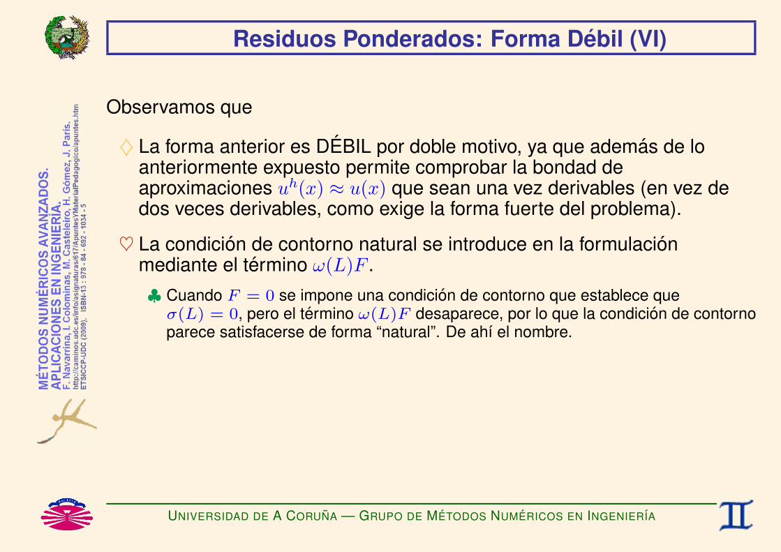
Residuos Ponderados: Forma Debil (VI)
Observamos que
♦ La forma anterior es DEBIL por doble motivo, ya que ademas de loanteriormente expuesto permite comprobar la bondad deaproximaciones uh(x) ≈ u(x) que sean una vez derivables (en vez dedos veces derivables, como exige la forma fuerte del problema).
♥ La condicion de contorno natural se introduce en la formulacionmediante el termino ω(L)F .♣ Cuando F = 0 se impone una condicion de contorno que establece queσ(L) = 0, pero el termino ω(L)F desaparece, por lo que la condicion de contornoparece satisfacerse de forma “natural”. De ahı el nombre.
UNIVERSIDAD DE A CORUNA — GRUPO DE METODOS NUMERICOS EN INGENIERIA
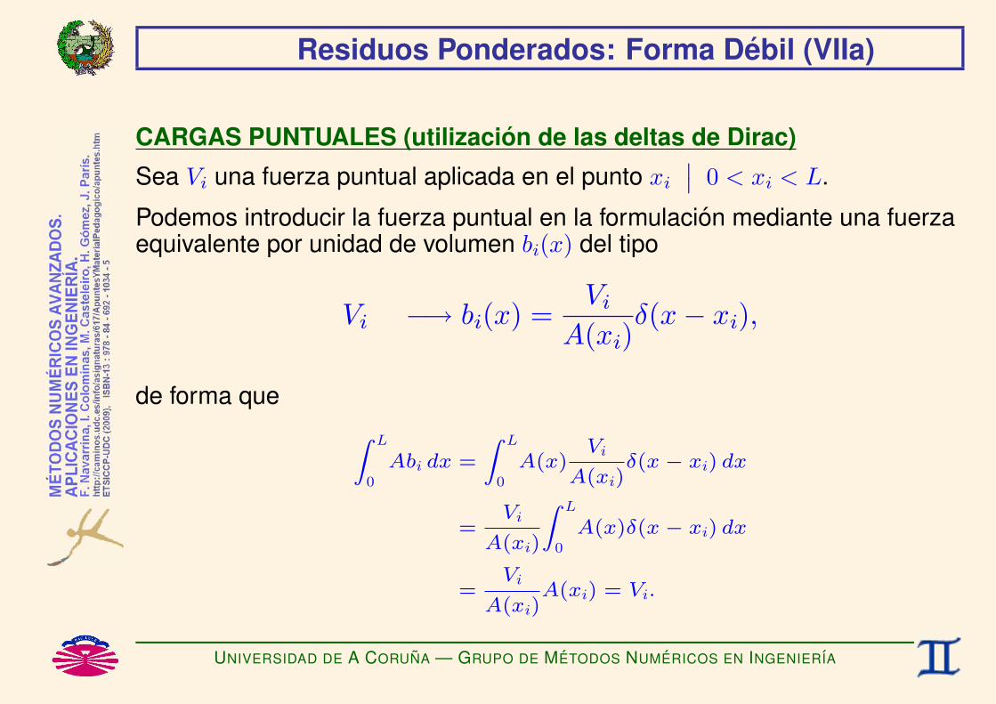
Residuos Ponderados: Forma Debil (VIIa)
CARGAS PUNTUALES (utilizacion de las deltas de Dirac)
Sea Vi una fuerza puntual aplicada en el punto xi∣∣ 0 < xi < L.
Podemos introducir la fuerza puntual en la formulacion mediante una fuerzaequivalente por unidad de volumen bi(x) del tipo
Vi −→ bi(x) =Vi
A(xi)δ(x− xi),
de forma que Z L
0
Abi dx =
Z L
0
A(x)Vi
A(xi)δ(x− xi) dx
=Vi
A(xi)
Z L
0
A(x)δ(x− xi) dx
=Vi
A(xi)A(xi) = Vi.
UNIVERSIDAD DE A CORUNA — GRUPO DE METODOS NUMERICOS EN INGENIERIA

Residuos Ponderados: Forma Debil (VIIb)
Al introducir bi(x) en la forma debil obtenemos∫ L
0
ωAbi dx =∫ L
0
ω(x)A(x)Vi
A(xi)δ(x− xi) dx
=Vi
A(xi)
∫ L
0
ω(x)A(x)δ(x− xi) dx
=Vi
A(xi)ω(xi)A(xi)
= ω(xi)Vi,
que es un termino del mismo tipo que los que corresponden a F y a R.
UNIVERSIDAD DE A CORUNA — GRUPO DE METODOS NUMERICOS EN INGENIERIA

Residuos Ponderados: Forma Debil (VIIIa)
EL PRINCIPIO DE LOS TRABAJOS VIRTUALES
♥ Si interpretamos la funcion de test ω(x) como un desplazamiento virtualcompatible con las condiciones de contorno esenciales (es decir comouna modificacion de la solucion u(x) que no incumpla las condiciones decontorno esenciales), e interpretamos su derivada como unadeformacion virtual, podemos escribir
ω(x) = δu(x) con δu(0) = 0, δε(x) =∂ω
∂x
y obtenemos el PRINCIPIO DE LOS TRABAJOS VIRTUALES∫ L
0
∂δu
∂xAσ dx =
∫ L
0
δuAb dx+ δu(L)F ∀δu(x)∣∣∣ δu(0) = 0.
♣ Por tanto, el PRINCIPIO DE LOS TRABAJOS VIRTUALES es unaforma debil de las ecuaciones de equilibrio (no de las ecuacionesconstitutivas ni de las de compatibilidad) y de las condiciones decontorno naturales (no de las condiciones de contorno esenciales).
UNIVERSIDAD DE A CORUNA — GRUPO DE METODOS NUMERICOS EN INGENIERIA

Residuos Ponderados: Forma Debil (VIIIb)
♥ El METODO DE RESIDUOS PONDERADOS permite obtener una formadebil del problema aunque no se conozca el enunciado especıfico delPTV para el problema que se esta resolviendo (por ejemplo, ¿quesignifica y como se escribe el principio de los trabajos virtuales enproblemas de difusion de contaminantes?)
♦ En el caso que nos ocupa (ecuacion de equilibrio de pequenosdesplazamientos, ecuacion de compatibilidad de pequenos gradientesde desplazamientos, ecuacion constitutiva de la elasticidad lineal), estaforma debil equivale al planteamiento variacional de mınima energıa, porlo que las soluciones numericas que proporcionara el metodo deGalerkin seran optimas. Esto no tiene por que ser cierto en otros casos(problemas de conveccion-difusion, dinamica de fluidos, etc.).
UNIVERSIDAD DE A CORUNA — GRUPO DE METODOS NUMERICOS EN INGENIERIA
Residuos Ponderados: Forma Debil (VIIIc)
♣ La forma clasica del bf PTV tambien es valida para ecuacionesconstitutivas no lineales (hiperelasticidad) y para ecuaciones decompatibilidad mas complicadas (grandes gradientes dedesplazamientos) siempre y cuando la ecuacion de equilibrio sea laexpuesta (pequenos desplazamientos). En todo caso, hay queinterpretar correctamente el enunciado y tener en cuenta que laexpresion de la deformacion virtual es siempre la correspondiente alcaso de pequenos gradientes de desplazamientos.
UNIVERSIDAD DE A CORUNA — GRUPO DE METODOS NUMERICOS EN INGENIERIA

Residuos Ponderados: Aproximacion Numerica (Ia)
FUNCIONES DE PRUEBA (Trial Functions)Sea la base de funciones de prueba φi(x)i=1,...,ν.
Dada la aproximacion inicial ψ(x), buscamos una mejor aproximacion
u(x) ≈ uh(x) = ψ(x) +ν∑i=1
αiφi(x), uh(x) ∈ Hhu ⊂ Hu,
u(x) ≈ uh(x) = ψ(x) + ΦT (x) α, con Φ(x) =
φ1(x)...φν(x)
, α =
α1...αν
.
Las correspondientes aproximaciones de ε(x) y de σ(x) seran
ε(x) ≈ εh(x) =
∂ψ
∂x+
νXi=1
αi∂φi
∂x, σ(x) ≈ σ
h(x) = Eε
h(x),
ε(x) ≈ εh(x) =
∂ψ
∂x+∂ΦT
∂xα, σ(x) ≈ σ
h(x) = Eε
h(x).
Y [si interesa] podemos buscar una aproximacion de la reaccion R ≈ Rh.
UNIVERSIDAD DE A CORUNA — GRUPO DE METODOS NUMERICOS EN INGENIERIA

Residuos Ponderados: Aproximacion Numerica (Ib)
En general no sera posible que uh(x) = u(x) ∀x ∈ [0, L] (*), por lo que
uh(x) 6= u(x)
m
no es posible queZ L
0
∂ω
∂xAσ
hdx =
Z L
0
ωAb dx+ ω(L)F + ω(0)Rh ∀ω(x) ∈ Hω.
(*) Salvo que u(x)− ψ(x) este contenido en el subespacio generado por las funciones de prueba.
UNIVERSIDAD DE A CORUNA — GRUPO DE METODOS NUMERICOS EN INGENIERIA
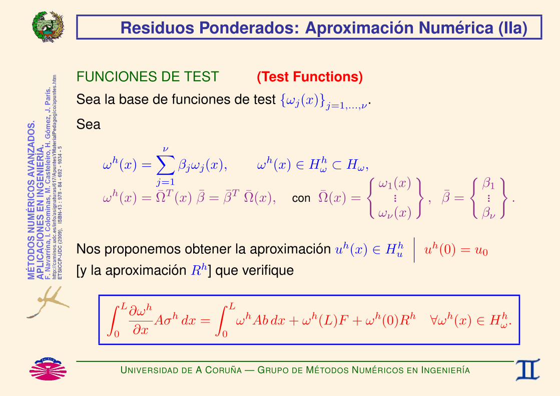
Residuos Ponderados: Aproximacion Numerica (IIa)
FUNCIONES DE TEST (Test Functions)
Sea la base de funciones de test ωj(x)j=1,...,ν.
Sea
ωh(x) =ν∑j=1
βjωj(x), ωh(x) ∈ Hhω ⊂ Hω,
ωh(x) = ΩT (x) β = βT Ω(x), con Ω(x) =
ω1(x)...ων(x)
, β =
β1...βν
.
Nos proponemos obtener la aproximacion uh(x) ∈ Hhu
∣∣∣ uh(0) = u0
[y la aproximacion Rh] que verifique
∫ L
0
∂ωh
∂xAσh dx =
∫ L
0
ωhAb dx+ ωh(L)F + ωh(0)Rh ∀ωh(x) ∈ Hhω.
UNIVERSIDAD DE A CORUNA — GRUPO DE METODOS NUMERICOS EN INGENIERIA

Residuos Ponderados: Aproximacion Numerica (IIb)
Pero Z L
0
∂ωh
∂xAσ
hdx−
Z L
0
ωhAb dx− ω
h(L)F − ω
h(0)R
h= 0 ∀ωh(x) ∈ Hh
ω
mνXj=1
βj
Z L
0
∂ωj
∂xAσ
hdx−
Z L
0
ωjAb dx− ωj(L)F − ωj(0)Rh
!= 0 ∀ βj
βT
Z L
0
∂Ω
∂xAσ
hdx−
Z L
0
ΩAb dx− Ω(L)F − Ω(0)Rh
!= 0 ∀β
mZ L
0
∂ωj
∂xAσ
hdx =
Z L
0
ωjAb dx+ ωj(L)F + ωj(0)Rh, j=1,...,νZ L
0
∂Ω
∂xAσ
hdx =
Z L
0
ΩAb dx+ Ω(L)F + Ω(0)Rh.
UNIVERSIDAD DE A CORUNA — GRUPO DE METODOS NUMERICOS EN INGENIERIA
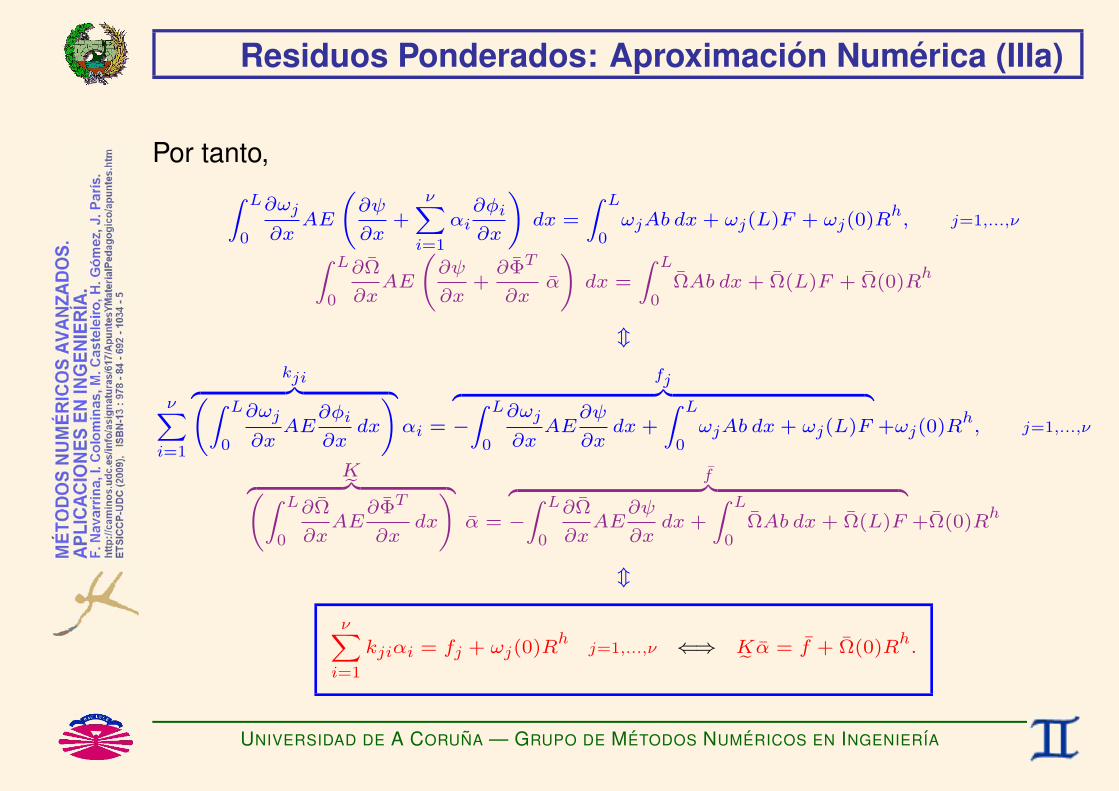
Residuos Ponderados: Aproximacion Numerica (IIIa)
Por tanto,Z L
0
∂ωj
∂xAE
∂ψ
∂x+
νXi=1
αi∂φi
∂x
!dx =
Z L
0ωjAb dx+ ωj(L)F + ωj(0)R
h, j=1,...,ν
Z L
0
∂Ω
∂xAE
∂ψ
∂x+∂ΦT
∂xα
!dx =
Z L
0ΩAb dx+ Ω(L)F + Ω(0)R
h
m
νXi=1
kjiz | Z L
0
∂ωj
∂xAE
∂φi
∂xdx
!αi =
fjz | −Z L
0
∂ωj
∂xAE
∂ψ
∂xdx+
Z L
0ωjAb dx+ ωj(L)F +ωj(0)R
h, j=1,...,ν
Kez | Z L
0
∂Ω
∂xAE
∂ΦT
∂xdx
!α =
fz | −Z L
0
∂Ω
∂xAE
∂ψ
∂xdx+
Z L
0ΩAb dx+ Ω(L)F +Ω(0)R
h
m
νXi=1
kjiαi = fj + ωj(0)Rh
j=1,...,ν ⇐⇒ Ke α = f + Ω(0)Rh.
UNIVERSIDAD DE A CORUNA — GRUPO DE METODOS NUMERICOS EN INGENIERIA

Residuos Ponderados: Aproximacion Numerica (IIIb)
Luego el problema de equilibrio original ha sido sustituido por el sistema(de orden ν, con la incognita adicional Rh)
K˜ α = f + Ω(0)Rh,
con la condicion adicional uh(0) = u0, esto es
ΦT (0) α = u0 − ψ(0).
UNIVERSIDAD DE A CORUNA — GRUPO DE METODOS NUMERICOS EN INGENIERIA
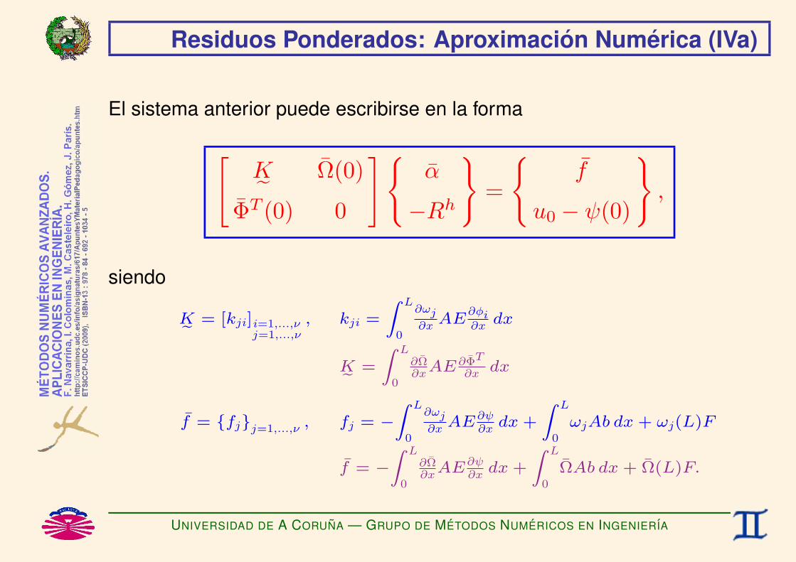
Residuos Ponderados: Aproximacion Numerica (IVa)
El sistema anterior puede escribirse en la forma[K˜ Ω(0)
ΦT (0) 0
] α
−Rh
=
f
u0 − ψ(0)
,
siendo
Ke = [kji]i=1,...,νj=1,...,ν
, kji =
Z L
0
∂ωj∂x AE
∂φi∂x dx
Ke =
Z L
0
∂Ω∂xAE
∂ΦT
∂x dx
f = fjj=1,...,ν , fj = −Z L
0
∂ωj∂x AE
∂ψ∂x dx+
Z L
0
ωjAb dx+ ωj(L)F
f = −Z L
0
∂Ω∂xAE
∂ψ∂x dx+
Z L
0
ΩAb dx+ Ω(L)F.
UNIVERSIDAD DE A CORUNA — GRUPO DE METODOS NUMERICOS EN INGENIERIA

Residuos Ponderados: Aproximacion Numerica (IVb)
Si elegimos la aproximacion inicial ψ(x) de forma que satisfaga la condicionde contorno esencial y elegimos las funciones de prueba φi(x) de forma quese anulen en el punto correspondiente, la aproximacion uh(x) verificaraautomaticamente la condicion de contorno esencial. Es decir
ψ(0) = u0
Φ(0) = 0
=⇒ uh(0) = u0.
Si ademas elegimos las funciones de test de forma que se anulen en elmismo punto, la reaccion no interviene en la formulacion y el sistema sereduce a
Ω(0) = 0 =⇒ K˜ α = f .
UNIVERSIDAD DE A CORUNA — GRUPO DE METODOS NUMERICOS EN INGENIERIA
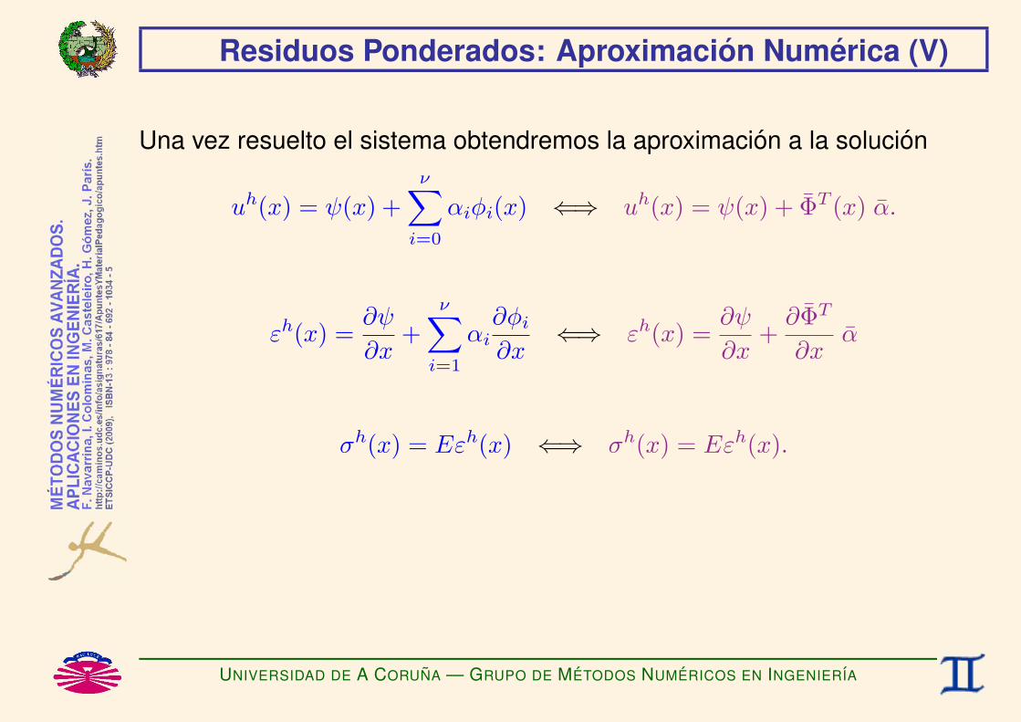
Residuos Ponderados: Aproximacion Numerica (V)
Una vez resuelto el sistema obtendremos la aproximacion a la solucion
uh(x) = ψ(x) +ν∑i=0
αiφi(x) ⇐⇒ uh(x) = ψ(x) + ΦT (x) α.
εh(x) =∂ψ
∂x+
ν∑i=1
αi∂φi∂x
⇐⇒ εh(x) =∂ψ
∂x+∂ΦT
∂xα
σh(x) = Eεh(x) ⇐⇒ σh(x) = Eεh(x).
UNIVERSIDAD DE A CORUNA — GRUPO DE METODOS NUMERICOS EN INGENIERIA
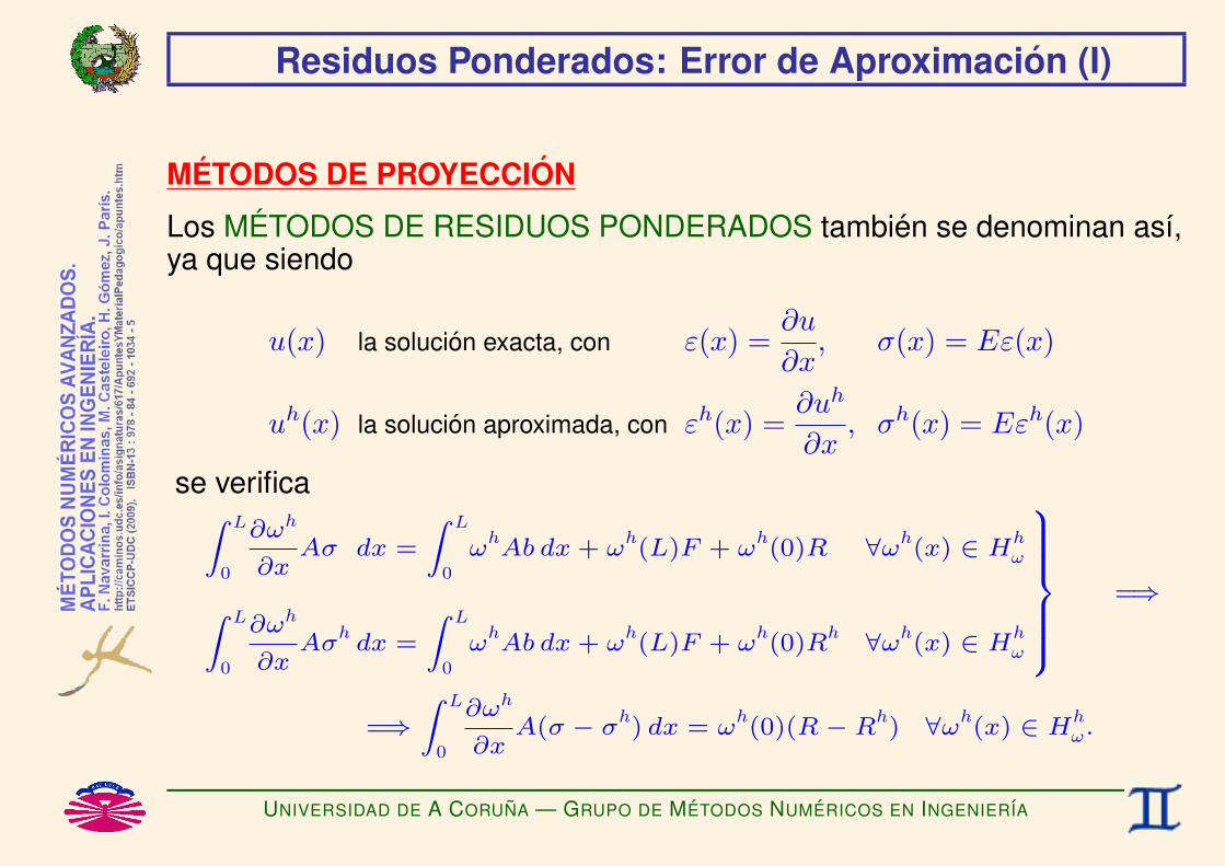
Residuos Ponderados: Error de Aproximacion (I)
METODOS DE PROYECCION
Los METODOS DE RESIDUOS PONDERADOS tambien se denominan ası,ya que siendo
u(x) la solucion exacta, con ε(x) =∂u
∂x, σ(x) = Eε(x)
uh(x) la solucion aproximada, con εh(x) =∂uh
∂x, σh(x) = Eεh(x)
se verificaZ L
0
∂ωh
∂xAσ dx =
Z L
0
ωhAb dx+ ω
h(L)F + ω
h(0)R ∀ωh(x) ∈ Hh
ω
Z L
0
∂ωh
∂xAσ
hdx =
Z L
0
ωhAb dx+ ω
h(L)F + ω
h(0)R
h ∀ωh(x) ∈ Hhω
9>>>>>=>>>>>;=⇒
=⇒Z L
0
∂ωh
∂xA(σ − σ
h) dx = ω
h(0)(R− R
h) ∀ωh(x) ∈ Hh
ω.
UNIVERSIDAD DE A CORUNA — GRUPO DE METODOS NUMERICOS EN INGENIERIA

Residuos Ponderados: Error de Aproximacion (II)
La ecuacion anterior demuestra que (normalmente) la reaccion se calculaexactamente, ya que si la funcion constante pertenece al espacio de lasfunciones de test (lo que normalmente se exige y se conoce comoPARTICION DE LA UNIDAD) entonces
ωh(x) = 1 =⇒ R = Rh .
Por tanto (normalmente) se cumpleZ L
0
∂ωh
∂xAE
∂
∂x(u− u
h) dx = 0 ∀ωh(x) ∈ Hh
ω.
Luego, la solucion aproximada uh(x) verifica
⟨ωh, u− uh
⟩= 0 ∀ωh(x) ∈ Hh
ω, con 〈v, e〉 =∫ L
0
∂v
∂xAE
∂e
∂xdx.
UNIVERSIDAD DE A CORUNA — GRUPO DE METODOS NUMERICOS EN INGENIERIA

Residuos Ponderados: Error de Aproximacion (III)
Por tanto, la solucion aproximada uh(x) es
la PROYECCION de la solucion exacta u(x)
sobre el subespacio Hhu de las funciones de prueba uh(x)
segun la normal al subespacio Hhω de las funciones de test ωh(x).
UNIVERSIDAD DE A CORUNA — GRUPO DE METODOS NUMERICOS EN INGENIERIA

Eleccion de las Funciones de Test
Algunas posibilidades. . .
1) METODO DE COLOCACION PUNTUAL
ωj(x) = δ(x− xj), j=1,...,ν con xj∈[0,L], xi 6=xj ∀i6=j. (*)
=⇒ No se puede utilizar en este caso, porque la delta no es derivable.Si se aplica a la forma original de RP conduce a DIFERENCIAS FINITAS.
2) METODO DE COLOCACION POR SUBDOMINIOS
ωj(x) = 1, si xj ≤ x ≤ xj+1,
0, en caso contrario, j=1,...,ν con a=x1≤...≤xν≤xν+1=b.
=⇒ Conduce a VOLUMENES FINITOS.
3) METODO DE BUBNOV-GALERKIN
ωj(x) = φj(x), j=1,...,ν ⇐⇒ Hhω = Hh
u .
(*) Si xj = a o xj = b es preciso redefinir adecuadamente la δ.
UNIVERSIDAD DE A CORUNA — GRUPO DE METODOS NUMERICOS EN INGENIERIA

Metodo de Bubnov-Galerkin (Ia)
PONDERACION DE BUBNOV–GALERKIN
Si se eligen como funciones de test las funciones de prueba, esto es
Hhω = Hh
u
mωj(x) = φj(x), j=0,...,ν ⇐⇒ Ω(x) = Φ(x),
se obtiene
Ke = [kji]i=1,...,νj=1,...,ν
, kji =
Z L
0
∂φj∂x AE
∂φi∂x dx
Ke =
Z L
0
∂Φ∂xAE
∂ΦT
∂x dx
f = fjj=1,...,ν , fj = −Z L
0
∂φj∂x AE
∂ψ∂x dx+
Z L
0
φjAb dx+ φj(L)F
f = −Z L
0
∂Φ∂xAE
∂ψ∂x dx+
Z L
0
ΦAb dx+ Φ(L)F.
UNIVERSIDAD DE A CORUNA — GRUPO DE METODOS NUMERICOS EN INGENIERIA
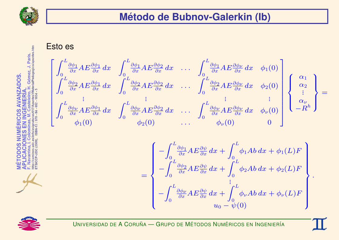
Metodo de Bubnov-Galerkin (Ib)
Esto es266666666664
Z L
0
∂φ1∂x AE
∂φ1∂x dx
Z L
0
∂φ1∂x AE
∂φ2∂x dx . . .
Z L
0
∂φ1∂x AE
∂φν∂x dx φ1(0)Z L
0
∂φ2∂x AE
∂φ1∂x dx
Z L
0
∂φ2∂x AE
∂φ2∂x dx . . .
Z L
0
∂φ2∂x AE
∂φν∂x dx φ2(0)
... ... ... ...Z L
0
∂φν∂x AE
∂φ1∂x dx
Z L
0
∂φν∂x AE
∂φ2∂x dx . . .
Z L
0
∂φν∂x AE
∂φν∂x dx φν(0)
φ1(0) φ2(0) . . . φν(0) 0
377777777775
8>>><>>>:α1
α2...αν−Rh
9>>>=>>>; =
=
8>>>>>>>>>><>>>>>>>>>>:
−Z L
0
∂φ1∂x AE
∂ψ∂x dx+
Z L
0
φ1Ab dx+ φ1(L)F
−Z L
0
∂φ2∂x AE
∂ψ∂x dx+
Z L
0
φ2Ab dx+ φ2(L)F
...
−Z L
0
∂φν∂x AE
∂ψ∂x dx+
Z L
0
φνAb dx+ φν(L)F
u0 − ψ(0)
9>>>>>>>>>>=>>>>>>>>>>;.
UNIVERSIDAD DE A CORUNA — GRUPO DE METODOS NUMERICOS EN INGENIERIA

Metodo de Bubnov-Galerkin (Ic)
Si elegimos
ψ(0) = u0
Φ(0) = 0
entonces la condicion de contorno esencial se verificara automaticamente yla reaccion no interviene en la formulacion con lo que el sistema se reduce a
K˜ α = f ,
siendo. . .
UNIVERSIDAD DE A CORUNA — GRUPO DE METODOS NUMERICOS EN INGENIERIA

Metodo de Bubnov-Galerkin (Id)
Ke =
2666666664
Z L
0
∂φ1∂x AE
∂φ1∂x dx
Z L
0
∂φ1∂x AE
∂φ2∂x dx . . .
Z L
0
∂φ1∂x AE
∂φν∂x dxZ L
0
∂φ2∂x AE
∂φ1∂x dx
Z L
0
∂φ2∂x AE
∂φ2∂x dx . . .
Z L
0
∂φ2∂x AE
∂φν∂x dx
... ... ...Z L
0
∂φν∂x AE
∂φ1∂x dx
Z L
0
∂φν∂x AE
∂φ2∂x dx . . .
Z L
0
∂φν∂x AE
∂φν∂x dx
3777777775
f =
8>>>>>>>><>>>>>>>>:
−Z L
0
∂φ1∂x AE
∂ψ∂x dx+
Z L
0
φ1Ab dx+ φ1(L)F
−Z L
0
∂φ2∂x AE
∂ψ∂x dx+
Z L
0
φ2Ab dx+ φ2(L)F
...
−Z L
0
∂φν∂x AE
∂ψ∂x dx+
Z L
0
φνAb dx+ φν(L)F
9>>>>>>>>=>>>>>>>>;.
UNIVERSIDAD DE A CORUNA — GRUPO DE METODOS NUMERICOS EN INGENIERIA

Metodo de Bubnov-Galerkin (II)
La solucion aproximada uh(x) verifica∫ L
0
∂φj∂x
Aσh dx−∫ L
0
φjAb dx− φj(L)F = 0
⇓
∂E
∂αj= 0, siendo E(α1, α2, . . . , αν) = E [uh],
por lo que se realiza un AJUSTE DE MINIMA ENERGIA.
UNIVERSIDAD DE A CORUNA — GRUPO DE METODOS NUMERICOS EN INGENIERIA

Metodo de Bubnov-Galerkin (IIIa)
La matriz K˜ del metodo de Galerkin es. . .
♥ SIMETRICAK˜ = K˜ T
♥ SEMIDEFINIDA POSITIVA
γTK˜ γ ≥ 0 ∀γ 6= 0
♥ DEFINIDA POSITIVA
γTK˜ γ > 0 ∀γ 6= 0 (*)
(*) Si la base de funciones de prueba ha sido correctamente elegida.
UNIVERSIDAD DE A CORUNA — GRUPO DE METODOS NUMERICOS EN INGENIERIA

Metodo de Bubnov-Galerkin (IIIb)
K˜ es SIMETRICA, ya que
kji =
Z L
0
∂φj
∂xAE
∂φi
∂xdx =
Z L
0
∂φi
∂xAE
∂φj
∂xdx = kij
m
Ke =
Z L
0
∂Φ
∂xAE
∂ΦT
∂xdx =
Z L
0
∂Φ
∂xAE
∂ΦT
∂x
!T
dx =
Z L
0
∂Φ
∂xAE
∂ΦT
∂xdx
!T
= Ke T .
UNIVERSIDAD DE A CORUNA — GRUPO DE METODOS NUMERICOS EN INGENIERIA
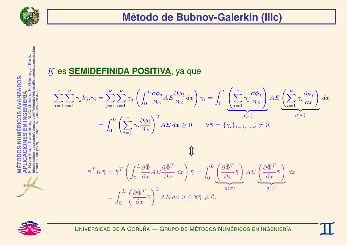
Metodo de Bubnov-Galerkin (IIIc)
K˜ es SEMIDEFINIDA POSITIVA, ya que
νXj=1
νXi=1
γjkjiγi =νXj=1
νXi=1
γj
Z L
0
∂φj
∂xAE
∂φi
∂xdx
!γi =
Z L
0
0@ νXj=1
γj∂φj
∂x
1A| z
g(x)
AE
νXi=1
γi∂φi
∂x
!| z
g(x)
dx
=
Z L
0
νXi=1
γi∂φi
∂x
!2
AE dx ≥ 0 ∀γ = γii=1,...,ν 6= 0.
m
γTKe γ = γ
T
Z L
0
∂Φ
∂xAE
∂ΦT
∂xdx
!γ =
Z L
0
∂ΦT
∂xγ
!| z
g(x)
AE
∂ΦT
∂xγ
!| z
g(x)
dx
=
Z L
0
∂ΦT
∂xγ
!2
AE dx ≥ 0 ∀γ 6= 0.
UNIVERSIDAD DE A CORUNA — GRUPO DE METODOS NUMERICOS EN INGENIERIA

Metodo de Bubnov-Galerkin (IIId)
K˜ es DEFINIDA POSITIVA, ya que (vease el punto anterior)
νXj=1
νXi=1
γjkjiγi = 0 =⇒νXi=1
γi∂φi
∂x= 0 ∀x ∈ [0, L] =⇒ γi = 0, i = 1, . . . , ν
m
γTKe γ = 0 =⇒
∂ΦT
∂xγ = 0 ∀x ∈ [0, L] =⇒ γ = 0.
si la base de funciones de prueba ha sido correctamente elegida (de formaque sus derivadas sean linealmente independientes).
UNIVERSIDAD DE A CORUNA — GRUPO DE METODOS NUMERICOS EN INGENIERIA

Metodo de Bubnov-Galerkin (IVa)
ESTIMACION DEL ERROR
Sabemos que la solucion aproximada uh(x) verifica
⟨ωh, u− uh
⟩= 0 ∀ωh(x) ∈ Hh
ω = Hhu , con 〈v, e〉 =
∫ L
0
∂v
∂xAE
∂e
∂xdx.
El producto escalar verifica la desigualdad de Cauchy
〈v, e〉 ≤ ‖v‖ ‖e‖ , con la norma ‖e‖ = 〈e, e〉12 =
√∫ L
0
(∂e∂x
)2
AE dx.
UNIVERSIDAD DE A CORUNA — GRUPO DE METODOS NUMERICOS EN INGENIERIA

Metodo de Bubnov-Galerkin (IVb)
APROXIMACION OPTIMA
La solucion aproximada uh(x) verifica
∥∥u− uh∥∥ ≤ ∥∥u− vh
∥∥ ∀vh ∈ Hhu .
UNIVERSIDAD DE A CORUNA — GRUPO DE METODOS NUMERICOS EN INGENIERIA

Metodo de Bubnov-Galerkin (IVc)
Pues,
uh, v
h ∈ Hhu =⇒ u
h − vh ∈ Hh
u =⇒Duh − v
h, u− u
hE
= 0,
luego
‚‚‚u− uh‚‚‚2
=Du− u
h, u− u
hE
+ 0 =Du− u
h, u− u
hE
+Duh − v
h, u− u
hE
=Du− u
h+ u
h − vh, u− u
hE
=Du− v
h, u− u
hE
≤‚‚‚u− v
h‚‚‚ ‚‚‚u− u
h‚‚‚ ,
y en consecuencia ‚‚‚u− uh‚‚‚ ≤ ‚‚‚u− v
h‚‚‚ .
UNIVERSIDAD DE A CORUNA — GRUPO DE METODOS NUMERICOS EN INGENIERIA

Metodo de Bubnov-Galerkin (IVd)
ESTIMACION DEL ERROR
Utilizando funciones de prueba vh ∈ Hhu adecuadamente elegidas se
pueden obtener cotas del error u− uh a partir de la expresion∥∥u− uh∥∥ ≤ ∥∥u− vh
∥∥ .
UNIVERSIDAD DE A CORUNA — GRUPO DE METODOS NUMERICOS EN INGENIERIA

Eleccion de las Funciones de Prueba (Ia)
Algunas posibilidades. . .
1) SOPORTE GLOBAL → METODO DE RITZ
♣ Ejemplos:B a) φi(x) = xi, i=1,...,ν→Hh
u = Pν(x).B b) Series de FourierB c) . . .
♠ Ke es LLENA → tiempo de computacion T (ν3).
♠ Ke puede ser MAL-CONDICIONADA. (*)
(*) EL numero de condicion depende de la base de funciones de prueba que se hayan elegido.
UNIVERSIDAD DE A CORUNA — GRUPO DE METODOS NUMERICOS EN INGENIERIA

Eleccion de las Funciones de Prueba (Ib)
2) SOPORTE LOCAL → METODO DE ELEMENTOS FINITOS
♣ Ejemplos:B a) Funciones en escalon.B b) Poligonales a trozos.B c) Splines en general.
♥ Se pretende que Ke sea SPARSE.
♥ Se pretende que Ke sea BIEN-CONDICIONADA.
UNIVERSIDAD DE A CORUNA — GRUPO DE METODOS NUMERICOS EN INGENIERIA

Notacion en Formas Bilineales (I)
FORMA DEBIL (Weak Form)
Hallar u(x) ∈ Hu
∣∣∣ u(0) = u0 [y R]
que VERIFICA a(ω, u) = (ω, b) + ω(L)F + ω(0)R ∀ω(x) ∈ Hω,
siendo a(ω, u) =∫ L
0
∂ω
∂xAE
∂u
∂xdx,
(ω, b) =∫ L
0
ωAb dx.
UNIVERSIDAD DE A CORUNA — GRUPO DE METODOS NUMERICOS EN INGENIERIA

Notacion en Formas Bilineales (IIa)
FUNCIONES DE PRUEBA (Trial Functions)
Sea la base de funciones de prueba φi(x)i=1,...,ν.
Dada la aproximacion inicial ψ(x), buscamos una mejor aproximacion
u(x) ≈ uh(x) = ψ(x) +ν∑i=1
αiφi(x), uh(x) ∈ Hhu ⊂ Hu,
u(x) ≈ uh(x) = ψ(x) + ΦT (x) α, con Φ(x) =
φ1(x)...φν(x)
, α =
α1...αν
.
Y [si interesa calcularla] podemos buscar una aproximacion de la reaccion
R ≈ Rh.
UNIVERSIDAD DE A CORUNA — GRUPO DE METODOS NUMERICOS EN INGENIERIA
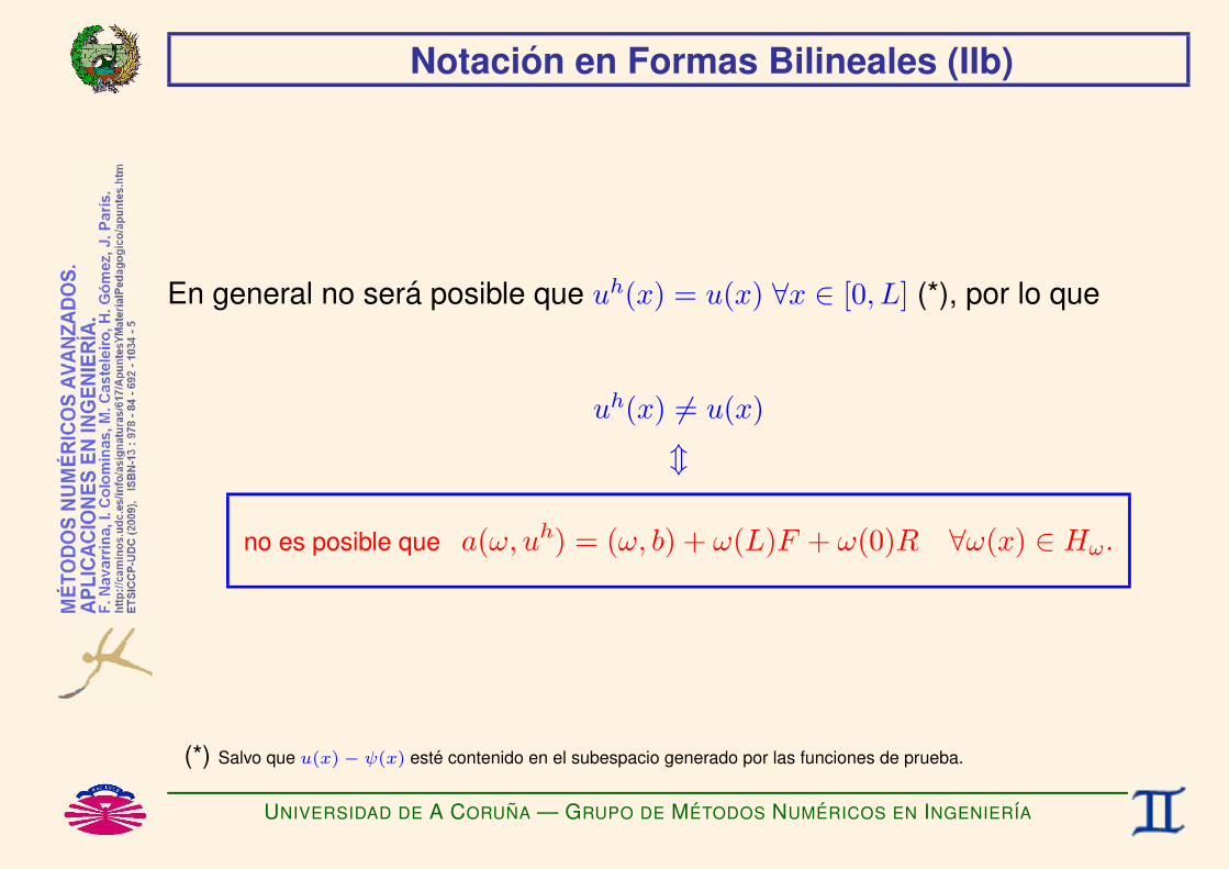
Notacion en Formas Bilineales (IIb)
En general no sera posible que uh(x) = u(x) ∀x ∈ [0, L] (*), por lo que
uh(x) 6= u(x)
m
no es posible que a(ω, uh) = (ω, b) + ω(L)F + ω(0)R ∀ω(x) ∈ Hω.
(*) Salvo que u(x)− ψ(x) este contenido en el subespacio generado por las funciones de prueba.
UNIVERSIDAD DE A CORUNA — GRUPO DE METODOS NUMERICOS EN INGENIERIA

Notacion en Formas Bilineales (IIIa)
FUNCIONES DE TEST (Test Functions)
Sea la base de funciones de test ωj(x)j=1,...,ν.
Sea
ωh(x) =ν∑j=1
βjωj(x), ωh(x) ∈ Hhω ⊂ Hω,
ωh(x) = ΩT (x) β = βT Ω(x), con Ω(x) =
ω1(x)...ων(x)
, β =
β1...βν
.
Nos proponemos obtener la aproximacion uh(x) ∈ Hhu
∣∣∣ uh(0) = u0
[y la aproximacion Rh] que verifique
a(ωh, uh) = (ωh, b) + ωh(L)F + ωh(0)Rh ∀ωh(x) ∈ Hhω.
UNIVERSIDAD DE A CORUNA — GRUPO DE METODOS NUMERICOS EN INGENIERIA

Notacion en Formas Bilineales (IIIb)
Pero
a(ωh, u
h)− (ω
h, b)− ω
h(L)F − ω
h(0)R
h= 0 ∀ωh(x) ∈ Hh
ω
mνXj=1
βj
„a(ωj, u
h)− (ωj, b)− ωj(L)F − ωj(0)R
h
«= 0 ∀ βj
βT„a(Ω, uh)− (Ω, b)− Ω(L)F − Ω(0)Rh
«= 0 ∀β
m
a(ωj, uh) = (ωj, b) + ωj(L)F + ωj(0)R
h, j=1,...,ν
a(Ω, uh) = (Ω, b) + Ω(L)F + Ω(0)R
h.
UNIVERSIDAD DE A CORUNA — GRUPO DE METODOS NUMERICOS EN INGENIERIA

Notacion en Formas Bilineales (IVa)
Por tanto,
a(ωj, ψ +
νXi=1
αiφi) = (ωj, b) + ωj(L)F + ωj(0)Rh
∀j
a(Ω, ψ + ΦT α) = (Ω, b) + Ω(L)F + Ω(0)Rh
m
νXi=1
kjiz | a(ωj, φi)αi =
fjz | −a(ωj, ψ) + (ωj, b) + ωj(L)F +ωj(0)R
h∀j
Kez | a(Ω, Φ
T) α =
fz | −a(Ω, ψ) + (Ω, b) + Ω(L)F +Ω(0)Rh
m
νXi=1
kjiαi = fj + ωj(0)Rh, j=1,...,ν ⇐⇒ Ke α = f + Ω(0)R
h.
UNIVERSIDAD DE A CORUNA — GRUPO DE METODOS NUMERICOS EN INGENIERIA
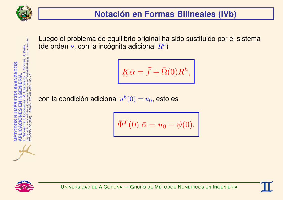
Notacion en Formas Bilineales (IVb)
Luego el problema de equilibrio original ha sido sustituido por el sistema(de orden ν, con la incognita adicional Rh)
K˜ α = f + Ω(0)Rh,
con la condicion adicional uh(0) = u0, esto es
ΦT (0) α = u0 − ψ(0).
UNIVERSIDAD DE A CORUNA — GRUPO DE METODOS NUMERICOS EN INGENIERIA
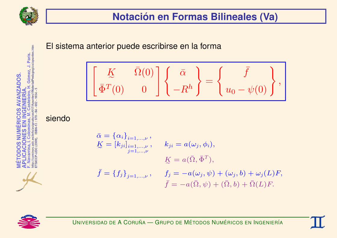
Notacion en Formas Bilineales (Va)
El sistema anterior puede escribirse en la forma[K˜ Ω(0)
ΦT (0) 0
] α
−Rh
=
f
u0 − ψ(0)
,
siendo
α = αii=1,...,ν ,Ke = [kji]i=1,...,ν
j=1,...,ν
, kji = a(ωj, φi),
Ke = a(Ω, ΦT ),
f = fjj=1,...,ν , fj = −a(ωj, ψ) + (ωj, b) + ωj(L)F,
f = −a(Ω, ψ) + (Ω, b) + Ω(L)F.
UNIVERSIDAD DE A CORUNA — GRUPO DE METODOS NUMERICOS EN INGENIERIA

Notacion en Formas Bilineales (Vb)
Si elegimos la aproximacion inicial ψ(x) de forma que satisfaga la condicionde contorno esencial y elegimos las funciones de prueba φi(x) de forma quese anulen en el punto correspondiente, la aproximacion uh(x) verificaraautomaticamente la condicion de contorno esencial. Es decir
ψ(0) = u0
Φ(0) = 0
=⇒ uh(0) = u0.
Si ademas elegimos las funciones de test de forma que se anulen en elmismo punto, la reaccion no interviene en la formulacion y el sistema sereduce a
Ω(0) = 0 =⇒ K˜ α = f .
UNIVERSIDAD DE A CORUNA — GRUPO DE METODOS NUMERICOS EN INGENIERIA
Notacion en Formas Bilineales (VI)
Una vez resuelto el sistema obtendremos la aproximacion a la solucion
uh(x) = ψ(x) +ν∑i=0
αiφi(x) ⇐⇒ uh(x) = ψ(x) + ΦT (x) α.
εh(x) =∂ψ
∂x+
ν∑i=1
αi∂φi∂x
⇐⇒ εh(x) =∂ψ
∂x+∂ΦT
∂xα
σh(x) = Eεh(x) ⇐⇒ σh(x) = Eεh(x).
UNIVERSIDAD DE A CORUNA — GRUPO DE METODOS NUMERICOS EN INGENIERIA
METODO DE RESIDUOS PONDERADOS:EJEMPLO DEL METODO DE RITZ
F. Navarrina, I. Colominas, M. Casteleiro, H. Gomez, J. Parıs
GMNI — GRUPO DE METODOS NUMERICOS EN INGENIERIA
Departamento de Metodos Matematicos y de RepresentacionEscuela Tecnica Superior de Ingenieros de Caminos, Canales y Puertos
Universidad de A Coruna, Espana
e-mail: [email protected] web: http://caminos.udc.es/gmni
UNIVERSIDAD DE A CORUNA — GRUPO DE METODOS NUMERICOS EN INGENIERIA

INDICE
I Problema Conceptual
I Solucion Analıtica
I Metodo de Ritz con ponderacion tipo Galerkin
I Solucion Numerica
UNIVERSIDAD DE A CORUNA — GRUPO DE METODOS NUMERICOS EN INGENIERIA

Problema Conceptual (I)
Sea el problema de equilibrio 1D:
UNIVERSIDAD DE A CORUNA — GRUPO DE METODOS NUMERICOS EN INGENIERIA

Problema Conceptual (II)
Pilar elastico a compresion de altura L
A(x) = A (seccion transversal constante).
b(x) = −ρg (peso propio, densidad constante).
F = −P (fuerza que soporta el pilar).
u0 = 0 (empotramiento perfecto en la base).
UNIVERSIDAD DE A CORUNA — GRUPO DE METODOS NUMERICOS EN INGENIERIA

Problema Conceptual (III)
Modelo Matematico Lineal:
Dados A, b = −ρg,E, u0, F = −P,Hallar u(x), σ(x), x ∈ [0, L], que verifican
∂
∂x(Aσ) +Ab = 0, (ECUACION DE EQUILIBRIO)
σ = Eε, (ECUACION CONSTITUTIVA)
ε =∂u
∂x, (ECUACION DE COMPATIBILIDAD)
−A(L)σ(L) + F = 0, (C.C. NATURAL)
u(0) = 0. (C.C. ESENCIAL)
UNIVERSIDAD DE A CORUNA — GRUPO DE METODOS NUMERICOS EN INGENIERIA

Solucion Analıtica (I)
Sustituyendo la ecuacion de compatibilidad en la constitutiva, y esta en la deequilibrio, obtenemos
∂
∂x
(AE
∂u
∂x
)−Aρg = 0 ∀x ∈ (0, L)
con
u(0) = 0,
∂u
∂x
∣∣∣∣x=L
= − P
AE.
UNIVERSIDAD DE A CORUNA — GRUPO DE METODOS NUMERICOS EN INGENIERIA

Solucion Analıtica (IIa)
La solucion analıtica del problema anterior es
u(x) = −∫ z=x
z=0
[1AE
(P +
∫ y=L
y=z
ρgAdy
)]dz,
ε(z) = − 1AE
(P +
∫ y=L
y=z
ρgAdy
),
σ(z) = − 1A
(P +
∫ y=L
y=z
ρgAdy
),
UNIVERSIDAD DE A CORUNA — GRUPO DE METODOS NUMERICOS EN INGENIERIA

Solucion Analıtica (IIb)
esto es,
u(x) = − 1K
[W
(x
L− 1
2
(xL
)2)
+ P(xL
)],
σ(x) = − 1A
[W(1− x
L
)+ P
],
donde
K =EA
L, W = ρgAL.
UNIVERSIDAD DE A CORUNA — GRUPO DE METODOS NUMERICOS EN INGENIERIA

Metodo de Ritz con ponderacion tipo Galerkin (I)
APROXIMACION INICIAL
ψ(x) = 0.
FUNCIONES DE PRUEBA
φi(x) =(xL
)i−1
, i=1,...,ν (RITZ).
Luego uh(x) es un polinomio de grado ν − 1.
FUNCIONES DE TEST
ωj(x) = φj(x), j=1,...,ν (GALERKIN).
UNIVERSIDAD DE A CORUNA — GRUPO DE METODOS NUMERICOS EN INGENIERIA
Metodo de Ritz con ponderacion tipo Galerkin (IIa)
Se obtiene
kji =
Z L
0
∂
∂x
„x
L
«j−1
AE∂
∂x
„x
L
«i−1
dx =
8>><>>:0 si i = 1 o j = 1,
(i− 1)(j − 1)
i + j − 3K si i 6= 1 y j 6= 1,
fj = −Z L
0
„x
L
«j−1
Aρgdx−„
x
L
«j−1˛˛x=L
P = −„
W
j+ P
«,
φi(0) =
„x
L
«j−1˛˛x=0
=
8<: 1 si j = 1,
0 si j 6= 1.
UNIVERSIDAD DE A CORUNA — GRUPO DE METODOS NUMERICOS EN INGENIERIA

Metodo de Ritz con ponderacion tipo Galerkin (IIb)
Esto es
0 0 . . . 0 10 K . . . K 0... ...
((i−1)(j−1)
i+j−3 K)
... ...
0 K . . . (ν−1)2
2ν−3 K 01 0 . . . 0 0
α1
α2...αν
−Rh
=
−(
W1 + P
)−(
W2 + P
)...
−(
Wν + P
)0
.
Luego,
Rh = W + P,
α1 = 0.
UNIVERSIDAD DE A CORUNA — GRUPO DE METODOS NUMERICOS EN INGENIERIA

Metodo de Ritz con ponderacion tipo Galerkin (IIc)
Por tanto, el sistema se reduce a. . .
K . . . K...
((i−1)(j−1)
i+j−3 K)
...
K . . . (ν−1)2
2ν−3 K
α2...αν
=
−(
W2 + P
)...
−(
Wν + P
) .
UNIVERSIDAD DE A CORUNA — GRUPO DE METODOS NUMERICOS EN INGENIERIA

Solucion Numerica (Ia)
ν = 2
[K ] α2 =−(
W2 + P
) ,
=⇒ α2 = − 1K
(W
2+ P
).
Luego,
uh(x) = α2φ2(x) = − 1K
(W
2+ P
)(xL
),
εh(x) =∂uh
∂x= − 1
EA
(W
2+ P
),
σh(x) = Eεh(x) = − 1A
(W
2+ P
).
UNIVERSIDAD DE A CORUNA — GRUPO DE METODOS NUMERICOS EN INGENIERIA

Solucion Numerica (Ib)
Comparamos la solucion numerica uh(x) con la solucion exacta u(x):
El error relativo en x = L2 es ru =
u(
L2
)− uh
(L2
)u(
L2
) =1
3 + 4 PW
.
Luego, PW = 10 −→ |ru| ≈ 2%.
UNIVERSIDAD DE A CORUNA — GRUPO DE METODOS NUMERICOS EN INGENIERIA

Solucion Numerica (Ic)
Comparamos la solucion numerica σh(x) con la solucion exacta σ(x):
El error relativo en x = L es rσ =σ(L)− σh(L)
σ(L)=
11 + 2 P
W
.
Luego, PW = 10 −→ |rσ| ≈ 5%.
UNIVERSIDAD DE A CORUNA — GRUPO DE METODOS NUMERICOS EN INGENIERIA

Solucion Numerica (Id)
OBSERVACIONES:
♥ Los desplazamientos se aproximan bien.
♣ Las tensiones se aproximan bien en promedio, pero peor que losdesplazamienos.♠ En general, las tensiones se aproximan mal localmente
(especialmente en los extremos).
♥ En algunos puntos la aproximacion de las tensiones puede ser exacta(normalmente en la zona central).
UNIVERSIDAD DE A CORUNA — GRUPO DE METODOS NUMERICOS EN INGENIERIA

Solucion Numerica (II)
ν = 3 [K K
K 43K
]α2
α3
=−(
W2 + P
)−(
W3 + P
) .=⇒ α2 = − 1
K(W + P ) , α3 =
1K
(W
2
).
Luego,
uh(x) = α2φ2(x) + α3φ3(x) = − 1K
[W
(x
L− 1
2
(xL
)2)
+ P(xL
)],
εh(x) =∂uh
∂x= − 1
EA
[W(1− x
L
)+ P
],
σh(x) = Eεh(x) = − 1A
[W(1− x
L
)+ P
].
que es la ¡SOLUCION EXACTA!
UNIVERSIDAD DE A CORUNA — GRUPO DE METODOS NUMERICOS EN INGENIERIA

Solucion Numerica (III)
ν = 4
K K K
K 43
32K
K 32K
95K
α2
α3
α4
=
−(
W2 + P
)−(
W3 + P
)−(
W4 + P
) .
=⇒ α2 = − 1K
(W + P ) , α3 =1K
(W
2
), α4 = 0.
Luego tambien se obtiene la ¡SOLUCION EXACTA!
Para ν ≥ 3 se obtiene siempre la solucion exacta porque u(x) ∈ Hhu . (*)
(*) La solucion exacta es un polinomio de segundo grado, y estamos aproximando la solucion mediante polinomios de gradoigual o superior a 2.
UNIVERSIDAD DE A CORUNA — GRUPO DE METODOS NUMERICOS EN INGENIERIA

INTRODUCCION AL METODO DE ELEMENTOS FINITOS:PROBLEMAS DE EQUILIBRIO 1D
F. Navarrina, I. Colominas, M. Casteleiro, H. Gomez, J. Parıs
GMNI — GRUPO DE METODOS NUMERICOS EN INGENIERIA
Departamento de Metodos Matematicos y de RepresentacionEscuela Tecnica Superior de Ingenieros de Caminos, Canales y Puertos
Universidad de A Coruna, Espana
e-mail: [email protected] web: http://caminos.udc.es/gmni
UNIVERSIDAD DE A CORUNA — GRUPO DE METODOS NUMERICOS EN INGENIERIA
INDICE
I Forma Debil
I Metodo de Elementos Finitos
UNIVERSIDAD DE A CORUNA — GRUPO DE METODOS NUMERICOS EN INGENIERIA

Forma Debil (I)
FORMA DEBIL (Residuos Ponderados + Integracion por partes)
Hallar u(x) ∈ Hu
∣∣∣ u(0) = u0 [y R]
que VERIFICA a(ω, u) = (ω, b) + ω(L)F + ω(0)R ∀ω(x) ∈ Hω,
siendo a(ω, u) =∫ L
0
∂ω
∂xAE
∂u
∂xdx,
(ω, b) =∫ L
0
ωAb dx.
UNIVERSIDAD DE A CORUNA — GRUPO DE METODOS NUMERICOS EN INGENIERIA

Forma Debil (II)
DISCRETIZACION FUNCIONAL
Funciones de Prueba: u(x) ≈ uh(x) ∈ Hhu ⊂ Hu
uh(x) = ψ(x)+ν∑i=1
αiφi(x)
= ψ(x)+ΦT (x) α, con Φ(x) =
φ1(x)...φν(x)
, α =
α1...αν
.
Funciones de Test: ω(x) → ωh(x) ∈ Hhω ⊂ Hω
ωh(x) =ν∑j=1
βjωj(x)
= βT Ω(x), con Ω(x) =
ω1(x)...ων(x)
, β =
β1...βν
.
UNIVERSIDAD DE A CORUNA — GRUPO DE METODOS NUMERICOS EN INGENIERIA

Forma Debil (III)
FORMA DEBIL DISCRETIZADA (RP+IP+Discretizacion Funcional)
Hallar uh(x) ∈ Hhu
∣∣∣ uh(0) = u0 [y Rh]
que VERIFICAa(ωh, uh) = (ωh, b) + ωh(L)F + ωh(0)Rh
∀ωh(x) ∈ Hhω,
siendo a(ω, u) =∫ L
0
∂ω
∂xAE
∂u
∂xdx,
(ω, b) =∫ L
0
ωAb dx.
UNIVERSIDAD DE A CORUNA — GRUPO DE METODOS NUMERICOS EN INGENIERIA

Forma Debil (IVa)
REDUCCION A UN SISTEMA ALGEBRAICO
Luego el problema de equilibrio original ha sido sustituido por el sistema(de orden ν, con la incognita adicional Rh)
K˜ α = f + Ω(0)Rh,
con la condicion adicional uh(0) = u0, esto es
ΦT (0) α = u0 − ψ(0).
UNIVERSIDAD DE A CORUNA — GRUPO DE METODOS NUMERICOS EN INGENIERIA
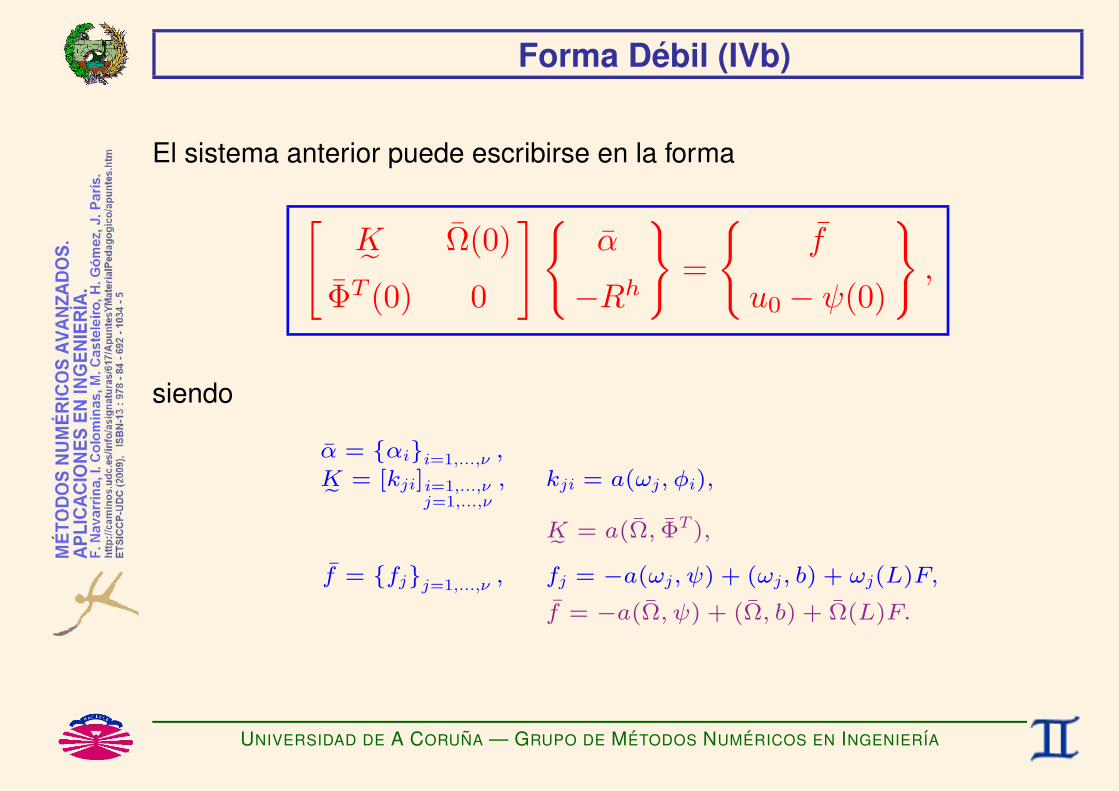
Forma Debil (IVb)
El sistema anterior puede escribirse en la forma[K˜ Ω(0)
ΦT (0) 0
] α
−Rh
=
f
u0 − ψ(0)
,
siendo
α = αii=1,...,ν ,Ke = [kji]i=1,...,ν
j=1,...,ν
, kji = a(ωj, φi),
Ke = a(Ω, ΦT ),
f = fjj=1,...,ν , fj = −a(ωj, ψ) + (ωj, b) + ωj(L)F,
f = −a(Ω, ψ) + (Ω, b) + Ω(L)F.
UNIVERSIDAD DE A CORUNA — GRUPO DE METODOS NUMERICOS EN INGENIERIA

Metodo de Elementos Finitos (I)
DISCRETIZACION DEL DOMINIO DE INTEGRACION
Diremos que el dominio [0, L] se ha discretizado en unaMALLA DE ELEMENTOS FINITOS si
[0, L] =N⋃e=1
Ee,Ee ∩
Ef= ∅ ∀e 6= f,
donde Ee es el ELEMENTO FINITO numero e.
Ejemplo:
Ee = [xe−1, xe], con a = x0 < x1 < . . . < xN = b.
UNIVERSIDAD DE A CORUNA — GRUPO DE METODOS NUMERICOS EN INGENIERIA

Metodo de Elementos Finitos (II)
Efecto: INTEGRACION ELEMENTO A ELEMENTO
∫ L
0
g(x) dx =N∑e=1
∫Ee
g(x) dx.
UNIVERSIDAD DE A CORUNA — GRUPO DE METODOS NUMERICOS EN INGENIERIA

Metodo de Elementos Finitos (III)
Luego
K˜ = a(Ω, ΦT ) =∫ L
0
∂Ω∂xAE
∂Φ∂x
dx
=N∑e=1
∫Ee
∂Ω∂xAE
∂Φ∂x
dx︸ ︷︷ ︸dK˜ e
.
f = −a(Ω, ψ) + (Ω, b) + Ω(L)F = −∫ L
0
∂Ω∂xAE
∂ψ
∂xdx+
∫ L
0
ωAb dx+ Ω(L)F
=N∑e=1
−∫Ee
∂Ω∂xAE
∂ψ
∂xdx+
∫Ee
ωAb dx︸ ︷︷ ︸bfe
+ Ω(L)F.
UNIVERSIDAD DE A CORUNA — GRUPO DE METODOS NUMERICOS EN INGENIERIA

METODO DE RESIDUOS PONDERADOS:EJEMPLO DEL METODO DE ELEMENTOS FINITOSF. Navarrina, I. Colominas, M. Casteleiro, H. Gomez, J. Parıs
GMNI — GRUPO DE METODOS NUMERICOS EN INGENIERIA
Departamento de Metodos Matematicos y de RepresentacionEscuela Tecnica Superior de Ingenieros de Caminos, Canales y Puertos
Universidad de A Coruna, Espana
e-mail: [email protected] web: http://caminos.udc.es/gmni
UNIVERSIDAD DE A CORUNA — GRUPO DE METODOS NUMERICOS EN INGENIERIA

INDICE
I Problema Conceptual
I Solucion Analıtica
I Formulacion MEF/Galerkin, 2 nodos/elemento
I Solucion MEF/Galerkin, 2 nodos/elemento
UNIVERSIDAD DE A CORUNA — GRUPO DE METODOS NUMERICOS EN INGENIERIA

Problema Conceptual (I)
Sea el problema de equilibrio 1D:
UNIVERSIDAD DE A CORUNA — GRUPO DE METODOS NUMERICOS EN INGENIERIA

Problema Conceptual (II)
Pilar elastico a compresion de altura L
A(x) = A (seccion transversal constante).
b(x) = −ρg (peso propio, densidad constante).
F = −P (fuerza que soporta el pilar).
u0 = 0 (empotramiento perfecto en la base).
UNIVERSIDAD DE A CORUNA — GRUPO DE METODOS NUMERICOS EN INGENIERIA

Problema Conceptual (III)
Modelo Matematico Lineal:
Dados A, b = −ρg,E, u0, F = −P,Hallar u(x), σ(x), x ∈ [0, L], que verifican
∂
∂x(Aσ) +Ab = 0, (ECUACION DE EQUILIBRIO)
σ = Eε, (ECUACION CONSTITUTIVA)
ε =∂u
∂x, (ECUACION DE COMPATIBILIDAD)
−A(L)σ(L) + F = 0, (C.C. NATURAL)
u(0) = 0. (C.C. ESENCIAL)
UNIVERSIDAD DE A CORUNA — GRUPO DE METODOS NUMERICOS EN INGENIERIA

Solucion Analıtica (I)
Sustituyendo la ecuacion de compatibilidad en la constitutiva, y esta en la deequilibrio, obtenemos
∂
∂x
(AE
∂u
∂x
)−Aρg = 0 ∀x ∈ (0, L)
con
u(0) = 0,
∂u
∂x
∣∣∣∣x=L
= − P
AE.
UNIVERSIDAD DE A CORUNA — GRUPO DE METODOS NUMERICOS EN INGENIERIA

Solucion Analıtica (IIa)
La solucion analıtica del problema anterior es
u(x) = −∫ z=x
z=0
[1AE
(P +
∫ y=L
y=z
ρgAdy
)]dz,
ε(z) = − 1AE
(P +
∫ y=L
y=z
ρgAdy
),
σ(z) = − 1A
(P +
∫ y=L
y=z
ρgAdy
),
UNIVERSIDAD DE A CORUNA — GRUPO DE METODOS NUMERICOS EN INGENIERIA

Solucion Analıtica (IIb)
esto es,
u(x) = − 1K
[W
(x
L− 1
2
(xL
)2)
+ P(xL
)],
σ(x) = − 1A
[W(1− x
L
)+ P
],
donde
K =EA
L, W = ρgAL.
UNIVERSIDAD DE A CORUNA — GRUPO DE METODOS NUMERICOS EN INGENIERIA

Formulacion MEF/Galerkin, 2 nodos/elemento (Ia)
APROXIMACION INICIAL
ψ(x) = 0.
DISCRETIZACION (Elementos de 2 nodos)
Nodos: xi =(i− 1ν − 1
)L, i=1,...,ν.
Elementos: Ee = [xe, xe+1], e=1,...,ν−1.
UNIVERSIDAD DE A CORUNA — GRUPO DE METODOS NUMERICOS EN INGENIERIA

Formulacion MEF/Galerkin, 2 nodos/elemento (Ib)
FUNCIONES DE PRUEBA
φi(x) =
(x− xi−1
xi − xi−1
)si x ∈ [xi−1, xi], i=2,...,ν(
x− xi+1
xi − xi+1
)si x ∈ [xi, xi+1], i=1,...,ν−1
0 en los casos restantes
(MEF).
FUNCIONES DE TEST
ωj(x) = φj(x), j=1,...,ν (GALERKIN).
UNIVERSIDAD DE A CORUNA — GRUPO DE METODOS NUMERICOS EN INGENIERIA

Formulacion MEF/Galerkin, 2 nodos/elemento (Ic)
Luego uh(x) =ν∑
i=1
αiφi(x) es una poligonal a trozos.
UNIVERSIDAD DE A CORUNA — GRUPO DE METODOS NUMERICOS EN INGENIERIA

Formulacion MEF/Galerkin, 2 nodos/elemento (IIa)
ORGANIZACION GLOBAL
kji =
Z L
0
∂φj(x)
∂xAE
∂φi(x)
∂xdx =
8>>>>>>><>>>>>>>:
(ν − 1)K si |i− j| = 0, i = 1 o i = ν,
2 (ν − 1)K si |i− j| = 0, i 6= 1 e i 6= ν,
−(ν − 1)K si |i− j| = 1,
0 en los casos restantes.
fj = −Z L
0
φj(x)Aρgdx− φj(L)P =
8>>>>>>>>>><>>>>>>>>>>:
−W
2(ν − 1)si j = 1,
−W
ν − 1si j 6= 1 y j 6= ν,
−W
2(ν − 1)− P si j = ν.
φi(0) =
8<: 1 si i = 1,
0 si i 6= 1.
UNIVERSIDAD DE A CORUNA — GRUPO DE METODOS NUMERICOS EN INGENIERIA

Formulacion MEF/Galerkin, 2 nodos/elemento (IIb)
Esto es266666666664
K∗ −K∗ 1
−K∗ 2K∗ −K∗ 0
−K∗ 2K∗ −K∗ 0. . . . . . . . . ...
−K∗ 2K∗ −K∗ 0
−K∗ K∗ 0
1 0 0 . . . 0 0 0
377777777775
8>>>>>>>>>><>>>>>>>>>>:
α1
α2
α3...
αν−1
αν
−Rh
9>>>>>>>>>>=>>>>>>>>>>;=
8>>>>>>>>>><>>>>>>>>>>:
−W ∗/2
−W ∗
−W ∗
...−W ∗
− (W ∗/2 + P )
0
9>>>>>>>>>>=>>>>>>>>>>;,
conK
∗= (ν − 1)K, W
∗=
W
ν − 1.
Luego,Rh = K∗(α1 − α2) +W ∗/2,
α1 = 0.
UNIVERSIDAD DE A CORUNA — GRUPO DE METODOS NUMERICOS EN INGENIERIA
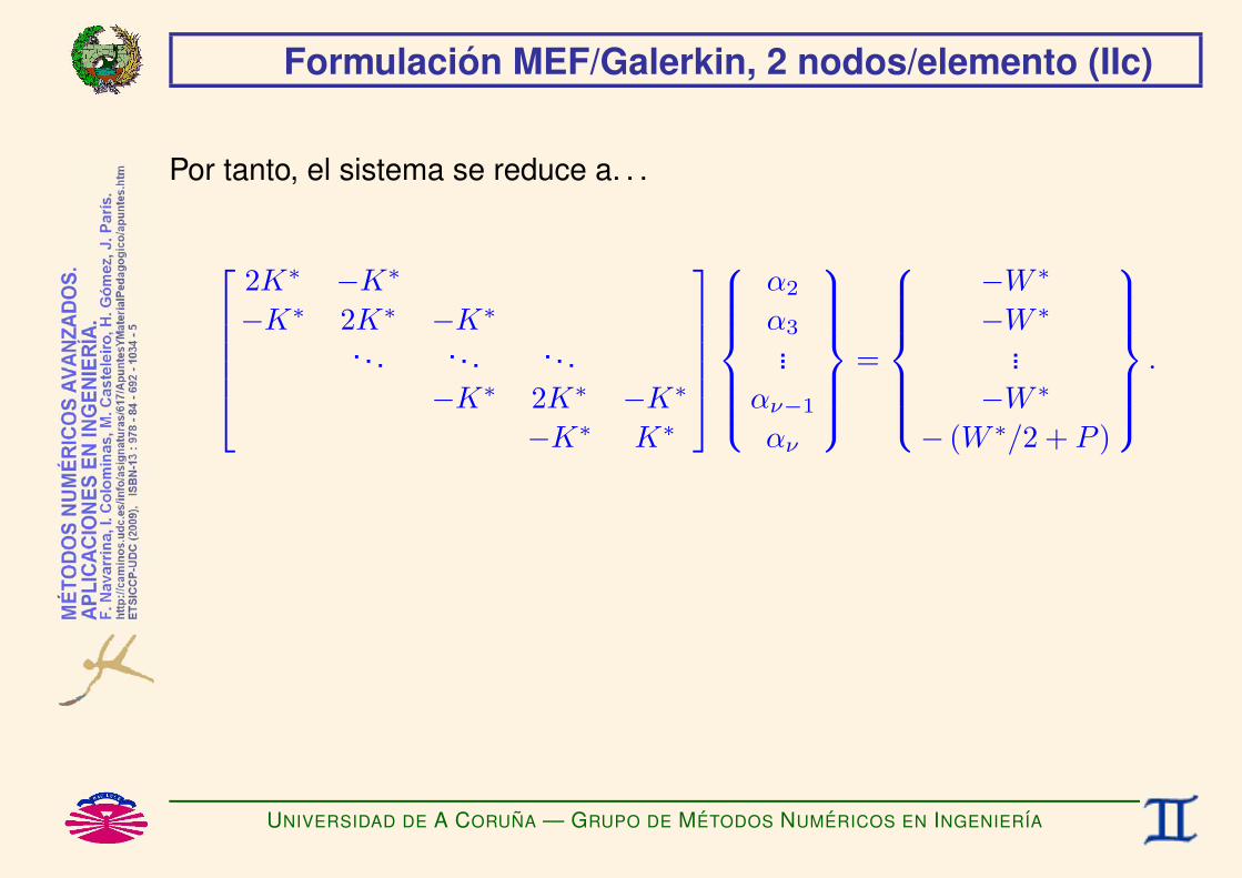
Formulacion MEF/Galerkin, 2 nodos/elemento (IIc)
Por tanto, el sistema se reduce a. . .
2K∗ −K∗
−K∗ 2K∗ −K∗
. . . . . . . . .−K∗ 2K∗ −K∗
−K∗ K∗
α2
α3...
αν−1
αν
=
−W ∗
−W ∗
...−W ∗
− (W ∗/2 + P )
.
UNIVERSIDAD DE A CORUNA — GRUPO DE METODOS NUMERICOS EN INGENIERIA

Formulacion MEF/Galerkin, 2 nodos/elemento (IIIa)
ORGANIZACION POR ELEMENTOS
Funciones de Forma
Sea el elemento
Ee = [xe1, x
e2]
donde xe1 = xe y xe
2 = xe+1 con la numeracion que hemos empleado.
Representamos las funciones de prueba a nivel de elemento mediante lasfunciones de forma
x ∈ Ee −→
φe (x) = N1(ξ) =
1− ξ
2,
φe+1(x) = N2(ξ) =1 + ξ
2,
UNIVERSIDAD DE A CORUNA — GRUPO DE METODOS NUMERICOS EN INGENIERIA
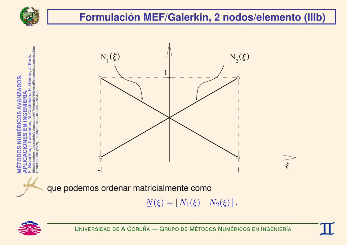
Formulacion MEF/Galerkin, 2 nodos/elemento (IIIb)
que podemos ordenar matricialmente como
N˜ (ξ) = [N1(ξ) N2(ξ) ] .
UNIVERSIDAD DE A CORUNA — GRUPO DE METODOS NUMERICOS EN INGENIERIA

Formulacion MEF/Galerkin, 2 nodos/elemento (IIIc)
Elementos isoparametricos
x(ξ) = N˜ (ξ)xe
1xe
2
= xe
1N1(ξ) + xe2N2(ξ).
El jacobiano de la transformacion geometrica es
dx
dξ= xe
1
∂N1(ξ)∂ξ
+ xe2
∂N2(ξ)∂ξ
= xe1
(−1
2
)+ xe
2
(12
)=xe
2 − xe1
2=he
2,
con
he = xe2 − xe
1.
UNIVERSIDAD DE A CORUNA — GRUPO DE METODOS NUMERICOS EN INGENIERIA

Formulacion MEF/Galerkin, 2 nodos/elemento (IIId)
Debemos calcular
B˜ = L˜N˜ , siendo L˜ =[∂
∂x
],
Pero [∂
∂x
]=dξ
dx
[∂
∂ξ
]donde
dξ
dx=(dx
dξ
)−1
=2he.
Luego [∂
∂x
]=
2he
[∂
∂ξ
].
UNIVERSIDAD DE A CORUNA — GRUPO DE METODOS NUMERICOS EN INGENIERIA

Formulacion MEF/Galerkin, 2 nodos/elemento (IIIe)
Por tanto
B˜ =[∂N1
∂x
∂N2
∂x
]=[
2he
∂N1
∂ξ
2he
∂N2
∂ξ
]=[
2he
(−1
2
)2he
(12
)]=
1he
[−1 1 ] .
Siendo
D˜ = [E]
ademas debemos calcular
K˜ e =∫ 1
−1
(B˜TD˜B˜)Adxdξdξ,
fe =∫ 1
−1
1− ξ
21 + ξ
2
(−ρg)Adxdξdξ.
UNIVERSIDAD DE A CORUNA — GRUPO DE METODOS NUMERICOS EN INGENIERIA
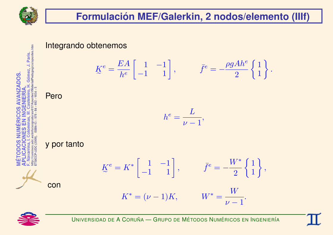
Formulacion MEF/Galerkin, 2 nodos/elemento (IIIf)
Integrando obtenemos
K˜ e =EA
he
[1 −1
−1 1
], fe = −ρgAh
e
2
11
.
Pero
he =L
ν − 1,
y por tanto
K˜ e = K∗[
1 −1−1 1
], fe = −W
∗
2
11
,
conK∗ = (ν − 1)K, W ∗ =
W
ν − 1.
UNIVERSIDAD DE A CORUNA — GRUPO DE METODOS NUMERICOS EN INGENIERIA

Formulacion MEF/Galerkin, 2 nodos/elemento (IIIg)
Finalmente, ensamblando y anadiendo las cargas puntuales y lascondiciones de contorno esenciales obtenemos el sistema266666666664
K∗ −K∗ 1
−K∗ 2K∗ −K∗ 0
−K∗ 2K∗ −K∗ 0. . . . . . . . . ...
−K∗ 2K∗ −K∗ 0
−K∗ K∗ 0
1 0 0 . . . 0 0 0
377777777775
8>>>>>>>>>><>>>>>>>>>>:
α1
α2
α3...
αν−1
αν
−Rh
9>>>>>>>>>>=>>>>>>>>>>;=
8>>>>>>>>>><>>>>>>>>>>:
−W ∗/2
−W ∗
−W ∗
...−W ∗
− (W ∗/2 + P )
0
9>>>>>>>>>>=>>>>>>>>>>;.
Comprobamos que el resultado es el mismo que se obtiene mediante laorganizacion global.
UNIVERSIDAD DE A CORUNA — GRUPO DE METODOS NUMERICOS EN INGENIERIA

Solucion MEF/Galerkin, 2 nodos/elemento (I)
ν = 2
[K∗ ] α2 = −W ∗ ,
=⇒ α2 = − 1K∗
(W ∗
2+ P
)= − 1
K
(W
2+ P
). (EXACTO)
Luego,u
h(x) = α2φ2(x) = −
1
K
„W
2+ P
« „x
L
«,
εh(x) =
∂uh
∂x= −
1
EA
„W
2+ P
«,
σh(x) = Eε
h(x) = −
1
A
„W
2+ P
«.
Es la solucion obtenida por Ritz utilizando un polinomio de grado 1.
UNIVERSIDAD DE A CORUNA — GRUPO DE METODOS NUMERICOS EN INGENIERIA

Solucion MEF/Galerkin, 2 nodos/elemento (IIa)
ν = 3 [2K∗ −K∗
−K∗ K∗
]α2
α3
=
−W ∗
−(W ∗/2 + P )
.
=⇒
α2 = − 1
K
(3W8
+P
2
), (EXACTO)
α3 = − 1K
(W
2+ P
). (EXACTO)
Luego,
uh(x) = α2φ2(x) + α3φ3(x),
εh(x) =∂uh
∂x,
σh(x) = Eεh(x).
UNIVERSIDAD DE A CORUNA — GRUPO DE METODOS NUMERICOS EN INGENIERIA

Solucion MEF/Galerkin, 2 nodos/elemento (IIb)
Comparamos la solucion numerica uh(x) con la solucion exacta u(x):
Se observa que la solucion numerica en los nodos es exacta.UNIVERSIDAD DE A CORUNA — GRUPO DE METODOS NUMERICOS EN INGENIERIA

Solucion MEF/Galerkin, 2 nodos/elemento (IIc)
Comparamos la solucion numerica σh(x) con la solucion exacta σ(x):
UNIVERSIDAD DE A CORUNA — GRUPO DE METODOS NUMERICOS EN INGENIERIA

Solucion MEF/Galerkin, 2 nodos/elemento (IIIa)
ν > 3
LOS VALORES NODALES DE LOS DESPLAZAMIENTOS EN ESTE CASOSON EXACTOS.
Este fenomeno se denomina SUPERCONVERGENCIA. (*)
(*) Por desgracia no es muy frecuente.
UNIVERSIDAD DE A CORUNA — GRUPO DE METODOS NUMERICOS EN INGENIERIA

Solucion MEF/Galerkin, 2 nodos/elemento (IIIb)
SUPERCONVERGENCIA
Recordemos que la solucion aproximada uh(x) verificaZ L
0
∂ωh
∂xAE
∂
∂x(u− u
h) dx = 0 ∀ω
h(x) ∈ H
hω.
Sea el punto x = z, z ∈ (0, L]. Si una de las posibles funciones de test fuese
ωh(x) =
8<:x
z, x ∈ [0, z]
1, x ∈ [z, L]
entonces Z z
0
1
zAE
∂
∂x(u− u
h) dx = 0.
En este caso AE = cte y uh(0) = u(0) = u0, luego
uh(z) = u(z).
Y, efectivamente, es posible elegir una funcion de test de ese tipo cuandox = z corresponde a un nodo.
UNIVERSIDAD DE A CORUNA — GRUPO DE METODOS NUMERICOS EN INGENIERIA
Solucion MEF/Galerkin, 2 nodos/elemento (IV)
OBSERVACIONES:
♥ Los desplazamientos se aproximan bien.
♣ Las tensiones se aproximan bien en promedio, pero peor que losdesplazamienos.♠ En general, las tensiones se aproximan mal localmente
(especialmente en los extremos).
♥ En algunos puntos la aproximacion de las tensiones puede ser exacta(normalmente en la zona central).
UNIVERSIDAD DE A CORUNA — GRUPO DE METODOS NUMERICOS EN INGENIERIA

METODO DE RESIDUOS PONDERADOS:PROBLEMAS DE EQUILIBRIO 2D/3D
F. Navarrina, I. Colominas, M. Casteleiro, H. Gomez, J. Parıs
GMNI — GRUPO DE METODOS NUMERICOS EN INGENIERIA
Departamento de Metodos Matematicos y de RepresentacionEscuela Tecnica Superior de Ingenieros de Caminos, Canales y Puertos
Universidad de A Coruna, Espana
e-mail: [email protected] web: http://caminos.udc.es/gmni
UNIVERSIDAD DE A CORUNA — GRUPO DE METODOS NUMERICOS EN INGENIERIA

INDICE
I Problema Conceptual
I Planteamientos Alternativos
I Residuos Ponderados: Forma Debil
I Residuos Ponderados: Aproximacion Numerica
I Residuos Ponderados: Error de Aproximacion
I Eleccion de las Funciones de Test
I Metodo de Bubnov-Galerkin
I Eleccion de las Funciones de Prueba
I Notacion en Formas Bilineales
UNIVERSIDAD DE A CORUNA — GRUPO DE METODOS NUMERICOS EN INGENIERIA

Problema Conceptual (I)
Sea el problema de equilibrio 2D/3D:
UNIVERSIDAD DE A CORUNA — GRUPO DE METODOS NUMERICOS EN INGENIERIA

Problema Conceptual (IIa)
ECUACION INTEGRAL DE EQUILIBRIO/CONSERVACION
∫∫∂V
σT n d(∂V ) = −∫∫∫
V
b dV ∀V.
Aplicando el Teorema de la DivergenciaZZ
∂V
σTn d(∂V ) =
ZZZV
div(σ) dV,
obtenemos ZZZV
“div(σ) + b
”dV = 0 ∀V.
UNIVERSIDAD DE A CORUNA — GRUPO DE METODOS NUMERICOS EN INGENIERIA

Problema Conceptual (IIb)
ECUACION DIFERENCIAL DE EQUILIBRIO (CONSERVACION)
div(σ) + b = 0.
UNIVERSIDAD DE A CORUNA — GRUPO DE METODOS NUMERICOS EN INGENIERIA
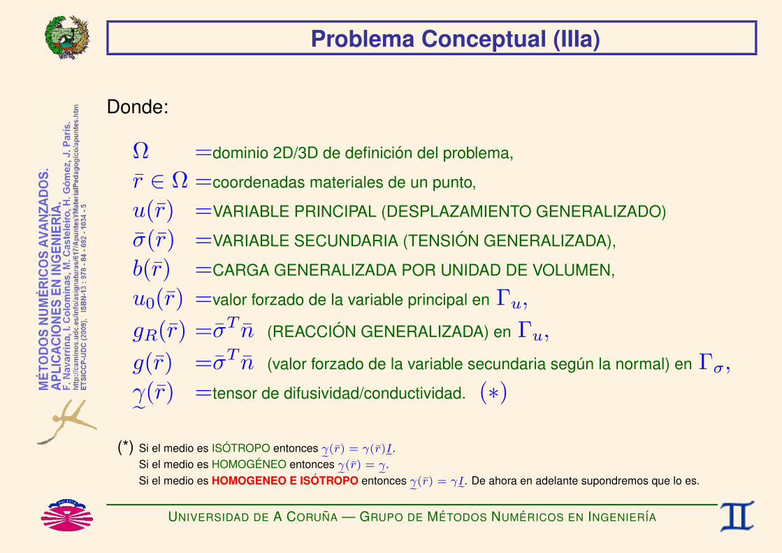
Problema Conceptual (IIIa)
Donde:
Ω =dominio 2D/3D de definicion del problema,
r ∈ Ω =coordenadas materiales de un punto,
u(r) =VARIABLE PRINCIPAL (DESPLAZAMIENTO GENERALIZADO)
σ(r) =VARIABLE SECUNDARIA (TENSION GENERALIZADA),
b(r) =CARGA GENERALIZADA POR UNIDAD DE VOLUMEN,
u0(r) =valor forzado de la variable principal en Γu,gR(r) =σT n (REACCION GENERALIZADA) en Γu,g(r) =σT n (valor forzado de la variable secundaria segun la normal) en Γσ,γ˜(r) =tensor de difusividad/conductividad. (∗)
(*) Si el medio es ISOTROPO entonces γe(r) = γ(r)Ie.Si el medio es HOMOGENEO entonces γe(r) = γe.Si el medio es HOMOGENEO E ISOTROPO entonces γe(r) = γIe. De ahora en adelante supondremos que lo es.
UNIVERSIDAD DE A CORUNA — GRUPO DE METODOS NUMERICOS EN INGENIERIA

Problema Conceptual (IIIb)
La relacion entre la variable principal u(r) y la variable secundaria σ(r) seestablece a traves de una variable intermedia ε(r) (DEFORMACIONGENERALIZADA), de forma que tendremos dos tipos de ecuaciones:
I ECUACIONES DE COMPATIBILIDAD(o relaciones deformacion—desplazamiento):
u(r) −→ ε(r).
I ECUACIONES CONSTITUTIVAS(o relaciones tension—deformacion):
ε(r) −→ σ(r).
UNIVERSIDAD DE A CORUNA — GRUPO DE METODOS NUMERICOS EN INGENIERIA

Problema Conceptual (IV)
Modelo Matematico Lineal (medio homogeneo e isotropo):
Dados b(r), γ(r), u0(r), g(r),
Hallar u(r), σ(r), r ∈ Ω, que verifican
div(σ) + b = 0 ∀r ∈Ω, (ECUACION DE EQUILIBRIO)
σ = −γε r ∈ Ω, (ECUACION CONSTITUTIVA)
ε = gradu r ∈ Ω, (ECUACION DE COMPATIBILIDAD)
− σT n+ g(r) = 0 ∀r ∈ Γσ, (C.C. NATURAL)
u = u0(r) ∀r ∈ Γu. (C.C. ESENCIAL)
El problema anterior puede representar diferentes fenomenos fısicos,como. . .
UNIVERSIDAD DE A CORUNA — GRUPO DE METODOS NUMERICOS EN INGENIERIA

Problema Conceptual (Va)
DEFORMACION DE UN MEDIO CONTINUO ELASTICO
I En este caso es necesario introducir• el TENSOR DE DEFORMACIONES y
• el TENSOR DE TENSIONES,
lo que obliga a realizar algunos ajustes en la formulacion anterior
I NO ANALIZAREMOS ESPECIFICAMENTE ESTE CASO porsimplicidad, pero en esencia los conceptos son los mismos.
En este caso, la ecuacion constitutiva se denomina LEY DE HOOKE.
UNIVERSIDAD DE A CORUNA — GRUPO DE METODOS NUMERICOS EN INGENIERIA

Problema Conceptual (Vb)
Difusion de contaminante en un medio 2D/3D
Ω =dominio 2D/3D de definicion del problema.
r ∈ Ω =coordenadas materiales de un punto.
u(r) =CONCENTRACION DE CONTAMINANTE.
ε(r) =GRADIENTE DE CONCENTRACION DE CONTAMINANTE.
σ(r) =DENSIDAD DE FLUJO DE CONTAMINANTE.
b(r) =SUMIDERO DE CONTAMINANTE POR UNIDAD DE VOLUMEN,
u0(r) =CONCENTRACION PREFIJADA en Γu,gR(r) =σT n (REACCION) en Γu,
g(r) =σT n (FLUJO DE CONTAMINANTE FORZADO) en Γσ.γ˜(r) =TENSOR DE DIFUSIVIDAD.
En este caso, la ecuacion constitutiva se denomina LEY DE FICKS.
UNIVERSIDAD DE A CORUNA — GRUPO DE METODOS NUMERICOS EN INGENIERIA

Problema Conceptual (Vc)
Difusion de calor en un medio 2D/3D
Ω =dominio 2D/3D de definicion del problema.
r ∈ Ω =coordenadas materiales de un punto.
u(r) =TEMPERATURA.
ε(r) =GRADIENTE DE TEMPERATURA.
σ(r) =DENSIDAD DE FLUJO DE CALOR.
b(r) =SUMIDERO DE CALOR POR UNIDAD DE VOLUMEN,
u0(r) =TEMPERATURA PREFIJADA en Γu,gR(r) =σT n (REACCION) en Γu,
g(r) =σT n (FLUJO DE CALOR FORZADO) en Γσ.γ˜(r) =TENSOR DE CONDUCTIVIDAD TERMICA.
En este caso, la ecuacion constitutiva se denomina LEY DE FOURIER.
UNIVERSIDAD DE A CORUNA — GRUPO DE METODOS NUMERICOS EN INGENIERIA

Problema Conceptual (Vd)
Corriente electrica en un medio conductor 2D/3D
Ω =dominio 2D/3D de definicion del problema.
r ∈ Ω =coordenadas materiales de un punto.
u(r) =POTENCIAL ELECTRICO.
ε(r) =GRADIENTE DE POTENCIAL.
σ(r) =DENSIDAD DE CORRIENTE.
b(r) =SUMIDERO DE CORRIENTE POR UNIDAD DE VOLUMEN,
u0(r) =POTENCIAL PREFIJADO en Γu,gR(r) =σT n (REACCION) en Γu,
g(r) =σT n (INTENSIDAD DE CORRIENTE FORZADA) en Γσ.γ˜(r) =TENSOR DE CONDUCTIVIDAD ELECTRICA.
En este caso, la ecuacion constitutiva se denomina LEY DE OHM.
UNIVERSIDAD DE A CORUNA — GRUPO DE METODOS NUMERICOS EN INGENIERIA

Planteamientos Alternativos (I)
a) FORMA ORIGINAL
Hallar u(r), r ∈ Ω,
tal que R(r) = 0 ∀r ∈Ω, RΓ(r) = 0 ∀r ∈ Γσ, (*)
siendo
R(r) = div(σ) + b r ∈Ω, (EC. DE EQUILIBRIO)
σ = −γε r ∈ Ω, (EC. CONSTITUTIVA)
ε = gradu r ∈ Ω, (EC. DE COMPATIBILIDAD)
RΓ(r) = −σT n+ g(r) r ∈ Γσ, (C.C. NATURAL)
u = u0(r) ∀r ∈ Γu. (C.C. ESENCIAL)
(*) FORMA FUERTE o STRONG FORM.
UNIVERSIDAD DE A CORUNA — GRUPO DE METODOS NUMERICOS EN INGENIERIA

Planteamientos Alternativos (IIa)
b) RESIDUOS PONDERADOS
Hallar u(r), r ∈ Ω,
tal que∫∫∫
r∈Ω
ω(r)R(r) dΩ +∫∫r∈Γσ
ωΓ(r)RΓ(r) dΓ = 0 ∀ω(r), ωΓ(r) (*)
siendo
R(r) = div(σ) + b r ∈Ω, (EC. DE EQUILIBRIO)
σ = −γε r ∈ Ω, (EC. CONSTITUTIVA)
ε = gradu r ∈ Ω, (EC. DE COMPATIBILIDAD)
RΓ(r) = −σT n+ g(r) r ∈ Γσ, (C.C. NATURAL)
u = u0(r) ∀r ∈ Γu. (C.C. ESENCIAL)
(*) FORMA DEBIL o WEAK FORM.
UNIVERSIDAD DE A CORUNA — GRUPO DE METODOS NUMERICOS EN INGENIERIA

Planteamientos Alternativos (IIb)
Pues
R = 0 ∀r ∈Ω, RΓ = 0∀r ∈ Γσ =⇒
ZZZr∈ΩωR dΩ +
ZZr∈Γσ
ωΓRΓ dΓ = 0 ∀ω, ωΓ
ZZZr∈ΩωR dΩ +
ZZr∈Γσ
ωΓRΓ dΓ = 0 ∀ω, ωΓ =⇒
8>>>><>>>>:ω = R, ωΓ = 0 →
ZZZr∈ΩR2
dΩ = 0,
ω = 0, ωΓ = RΓ →ZZr∈Γσ
R2Γ dΓ = 0.
♥ Si las funciones son suficientemente regulares, el enunciado de residuosponderados es equivalente al problema original, ya queZZZ
r∈ΩR2
dΩ = 0 =⇒R(r) = 0 ∀r ∈Ω,ZZ
r∈ΓσR2
Γ dΓ = 0 =⇒RΓ(r) = 0 ∀r ∈ Γσ.
♣ Si se utiliza la Integral de Lebesgue, los residuos R(r) y RΓ(r)pueden ser nonulos en un conjunto de puntos de medida nula. (*)
(*) Por este motivo se habla de una FORMULACION DEBIL (WEAK FORMULATION) del problema original.
UNIVERSIDAD DE A CORUNA — GRUPO DE METODOS NUMERICOS EN INGENIERIA

Planteamientos Alternativos (IIc)
Sin perdida de generalidad podemos elegir
ωΓ = ω(r) r ∈ Γσ,
puesR = 0 ∀r ∈
Ω, RΓ = 0 ∀r ∈ Γσ =⇒
ZZZr∈ΩωR dΩ +
ZZr∈Γσ
ωRΓ = 0 ∀ω
ZZZr∈ΩωR dΩ +
ZZr∈Γσ
ωRΓ dΓ = 0 ∀ω =⇒
8><>:ω = R ∗ P →R = 0 ∀r ∈
Ω, (∗)
R = 0, ω = RΓ →RΓ = 0 ∀r ∈ Γσ.
(*) donde P(r) es cualquier funcion que cumpla
P(r) > 0 ∀r ∈Ω, P(r) = 0 ∀r ∈ Γσ,
pues si las funciones son suficientemente regulares,ZZZr∈ΩR2
>0z|P dΩ = 0 =⇒R(r) = 0 ∀r ∈
Ω,ZZ
r∈ΓσR2
Γ dΓ = 0 =⇒RΓ(r) = 0 ∀r ∈ Γσ.
UNIVERSIDAD DE A CORUNA — GRUPO DE METODOS NUMERICOS EN INGENIERIA

Planteamientos Alternativos (IId)
Por tanto, podemos adoptar el enunciado de residuos ponderados. . .
Hallar u(r), r ∈ Ω,
tal que∫∫∫
r∈Ω
ω(r)R(r) dΩ +∫∫r∈Γσ
ω(r)RΓ(r) dΓ = 0 ∀ω(r)
siendo
R(r) = div(σ) + b r ∈Ω, (EC. DE EQUILIBRIO)
σ = −γε r ∈ Ω, (EC. CONSTITUTIVA)
ε = gradu r ∈ Ω, (EC. DE COMPATIBILIDAD)
RΓ(r) = −σT n+ g(r) r ∈ Γσ, (C.C. NATURAL)
u = u0(r) ∀r ∈ Γu. (C.C. ESENCIAL)
UNIVERSIDAD DE A CORUNA — GRUPO DE METODOS NUMERICOS EN INGENIERIA

Planteamientos Alternativos (IIIa)
c) MINIMOS CUADRADOS
Hallar u(r), r ∈ Ω,
que MINIMIZA Q[u] =∫∫∫
r∈Ω
R(r)p(r)R(r) dΩ +∫∫r∈Γσ
RΓ(r)pΓ(r)RΓ(r) dΓ, (*)
siendo
R(r) = div(σ) + b r ∈Ω, (EC. DE EQUILIBRIO)
σ = −γε r ∈ Ω, (EC. CONSTITUTIVA)
ε = gradu r ∈ Ω, (EC. DE COMPATIB.)
RΓ(r) = −σT n+ g(r) r ∈ Γσ, (C.C. NATURAL)
u = u0(r) ∀r ∈ Γu. (C.C. ESENCIAL)
(*) Las funciones de peso p(r) y pΓ(r) deben verificar p(r) > 0 ∀r ∈ Ω, pΓ(r) > 0 ∀r ∈ Γσ.
UNIVERSIDAD DE A CORUNA — GRUPO DE METODOS NUMERICOS EN INGENIERIA

Planteamientos Alternativos (IIIb)
La condicion de mınimo equivale al PLANTEAMIENTO VARIACIONAL
Hallar u(r) r ∈ Ω,
tal quedJ(λ)dλ
∣∣∣∣λ=0
= 0 ∀δu(r) con δu(r) = 0 en Γu,
con J(λ) = Q[u+ λδu],
y por tantodJ(λ)dλ
∣∣∣∣λ=0
= 2∫∫∫
r∈Ω
div(−γ grad δu)p(r)R(r) dΩ
− 2∫∫r∈Γσ
(−γ grad δu)T n pΓ(r)RΓ(r) dΓ, (*)
UNIVERSIDAD DE A CORUNA — GRUPO DE METODOS NUMERICOS EN INGENIERIA

Planteamientos Alternativos (IIIc)
. . . que equivale a decir
Hallar u(r) r ∈ Ω,
tal que
∫∫∫r∈Ω
div(−γ grad δu)p(r)R(r) dΩ
−∫∫r∈Γσ
(−γ grad δu)T n pΓ(r)RΓ(r) dΓ = 0 ∀δu(r) = 0 en Γu,
siendo
R(r) = div(σ) + b r ∈Ω, (EC. DE EQUILIBRIO)
σ = −γε r ∈ Ω, (EC. CONSTITUTIVA)
ε = gradu r ∈ Ω, (EC. DE COMPATIB.)
RΓ(r) = −σT n+ g(r) r ∈ Γσ, (C.C. NATURAL)
u = u0(r) ∀r ∈ Γu. (C.C. ESENCIAL)
UNIVERSIDAD DE A CORUNA — GRUPO DE METODOS NUMERICOS EN INGENIERIA

Planteamientos Alternativos (IIId)
. . . o lo que es lo mismoHallar u(r) r ∈ Ω,
tal que
∫∫∫r∈Ω
ω(r)R(r) dΩ +∫∫r∈Γσ
ωΓ(r)RΓ(r) = 0 ∀δu(r)∣∣∣ δu(0) = 0,
ω(r) = div(−γ grad δu)p(r), ωΓ(r) = −(−γ grad δu)T n pΓ(r),(*)
siendo
R(r) = div(σ) + b r ∈Ω, (EC. DE EQUILIBRIO)
σ = −γε r ∈ Ω, (EC. CONSTITUTIVA)
ε = gradu r ∈ Ω, (EC. DE COMPATIB.)
RΓ(r) = −σT n+ g(r) r ∈ Γσ, (C.C. NATURAL)
u = u0(r) ∀r ∈ Γu. (C.C. ESENCIAL)
(*) Que es un planteamiento en residuos ponderados equivalente al problema original.
UNIVERSIDAD DE A CORUNA — GRUPO DE METODOS NUMERICOS EN INGENIERIA

Planteamientos Alternativos (IVa)
e) MINIMA ENERGIA
Hallar u(r), r ∈ Ω,
que MINIMIZA
E [u] =− 12
∫∫∫r∈Ω
ε(r)T σ(r) dΩ
+∫∫∫
r∈Ω
u(r)b(r) dΩ +∫∫r∈Γσ
u(r)g(r) dΓ,
(*)
siendo
σ = −γε r ∈ Ω, (ECUACION CONSTITUTIVA)
ε = gradu, r ∈ Ω, (ECUACION DE COMPATIBILIDAD)
u = u0(r) ∀r ∈ Γu. (C.C. ESENCIAL)
UNIVERSIDAD DE A CORUNA — GRUPO DE METODOS NUMERICOS EN INGENIERIA

Planteamientos Alternativos (IVb)
Se comprueba facilmente que la solucion del problema original u(r)minimiza la energıa, pues si v(r) = u(r) + δu(r) es cualquier otra funcionque tambien verifique la condicion de contorno esencial v(0) = u0, entoncesδu(0) = 0, y siendo
δε =∂δu
∂x, δσ = Eδε,
tenemos
E[u+ δu] = −1
2
ZZZr∈Ω
(ε+ δε)T(σ + δσ) dΩ +
ZZZr∈Ω
(u+ δu)b dΩ +
ZZr∈Γσ
(u+ δu)g dΓ
= E[u]−1
2
ZZZr∈Ω
(δεTσ + ε
Tδσ + δε
Tδσ) dΩ +
ZZZr∈Ω
δub dΩ +
ZZr∈Γσ
δug dΓ
= E[u] +1
2
ZZZr∈Ω
(δεTγε+ ε
Tγδε+ δε
Tγδε) dΩ +
ZZZr∈Ω
δub dΩ +
ZZr∈Γσ
δug dΓ
= E[u] +1
2
ZZZr∈Ω
δεT(γδε) dΩ
+
»−ZZZ
r∈Ω
δεTσ dΩ +
ZZZr∈Ω
δub dΩ +
ZZr∈Γσ
δug dΓ
–.
UNIVERSIDAD DE A CORUNA — GRUPO DE METODOS NUMERICOS EN INGENIERIA

Planteamientos Alternativos (IVc1)
Perodiv(δuσ) = grad
T(δu)| z
δεT
σ + δu div σ.
Luego ZZZr∈Ω
δεTσ dΩ =
ZZZr∈Ω
div(δuσ) dΩ−ZZZ
r∈Ω
δu div σ dΩ.
Y aplicando el TEOREMA DE LA DIVERGENCIA,ZZZr∈Ω
δεTσ dΩ =
ZZr∈Γ
(δuσ)Tn dΓ−
ZZZr∈Ω
δu div σ dΩ.
UNIVERSIDAD DE A CORUNA — GRUPO DE METODOS NUMERICOS EN INGENIERIA
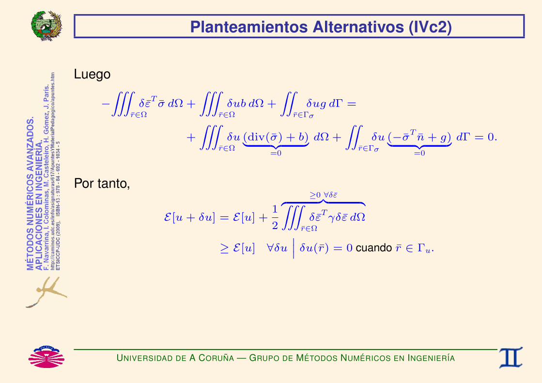
Planteamientos Alternativos (IVc2)
Luego
−ZZZ
r∈Ω
δεTσ dΩ +
ZZZr∈Ω
δub dΩ +
ZZr∈Γσ
δug dΓ =
+
ZZZr∈Ω
δu (div(σ) + b)| z =0
dΩ +
ZZr∈Γσ
δu (−σT n+ g)| z =0
dΓ = 0.
Por tanto,
E[u+ δu] = E[u] +1
2
≥0 ∀δεz | ZZZr∈Ω
δεTγδε dΩ
≥ E[u] ∀δu˛δu(r) = 0 cuando r ∈ Γu.
UNIVERSIDAD DE A CORUNA — GRUPO DE METODOS NUMERICOS EN INGENIERIA

Planteamientos Alternativos (IVd)
La condicion de mınimo equivale al PLANTEAMIENTO VARIACIONAL
Hallar u(r), r ∈ Ω,
tal quedJ(λ)dλ
∣∣∣∣λ=0
= 0 ∀δu tal que δu(r) = 0 cuando r ∈ Γu,
con J(λ) = E [u+ λδu],
y por tantodJ(λ)dλ
∣∣∣∣λ=0
= +∫∫∫
r∈Ω
gradT(δu)γ grad(u) dΩ
+∫∫∫
r∈Ω
δub dΩ +∫∫r∈Γσ
ug dΓ,
UNIVERSIDAD DE A CORUNA — GRUPO DE METODOS NUMERICOS EN INGENIERIA

Planteamientos Alternativos (IVe)
. . . que conduce al PRINCIPIO DE LOS TRABAJOS VIRTUALES (PTV)
Hallar u(r), r ∈ Ω,
tal que
+∫∫∫
r∈Ω
gradT(δu)σ dΩ
−∫∫∫
r∈Ω
δub dΩ
−∫∫r∈Γσ
δug dΓ = 0 ∀δu∣∣∣ δu(r) = 0 cuando r ∈ Γu,
siendo
σ = −γε r ∈ Ω, (ECUACION CONSTITUTIVA)
ε = gradu, r ∈ Ω, (ECUACION DE COMPATIBILIDAD)
u = u0(r) ∀r ∈ Γu. (C.C. ESENCIAL)
UNIVERSIDAD DE A CORUNA — GRUPO DE METODOS NUMERICOS EN INGENIERIA

Planteamientos Alternativos (IVf1)
Pero
gradT(δu)σ = div(δuσ)− δu div(σ).
Y, por tanto,ZZZr∈Ω
gradT(δu)σ dΩ =
ZZZr∈Ω
div(δuσ) dΩ−ZZZ
r∈Ω
δu div(σ) dΩ.
Aplicando el teorema de la divergencia,
ZZZr∈Ω
div(δuσ) dΩ =
ZZr∈Γ
(δuσ)Tn dΓ
=
ZZr∈Γ
δu(σTn) dΓ.
UNIVERSIDAD DE A CORUNA — GRUPO DE METODOS NUMERICOS EN INGENIERIA
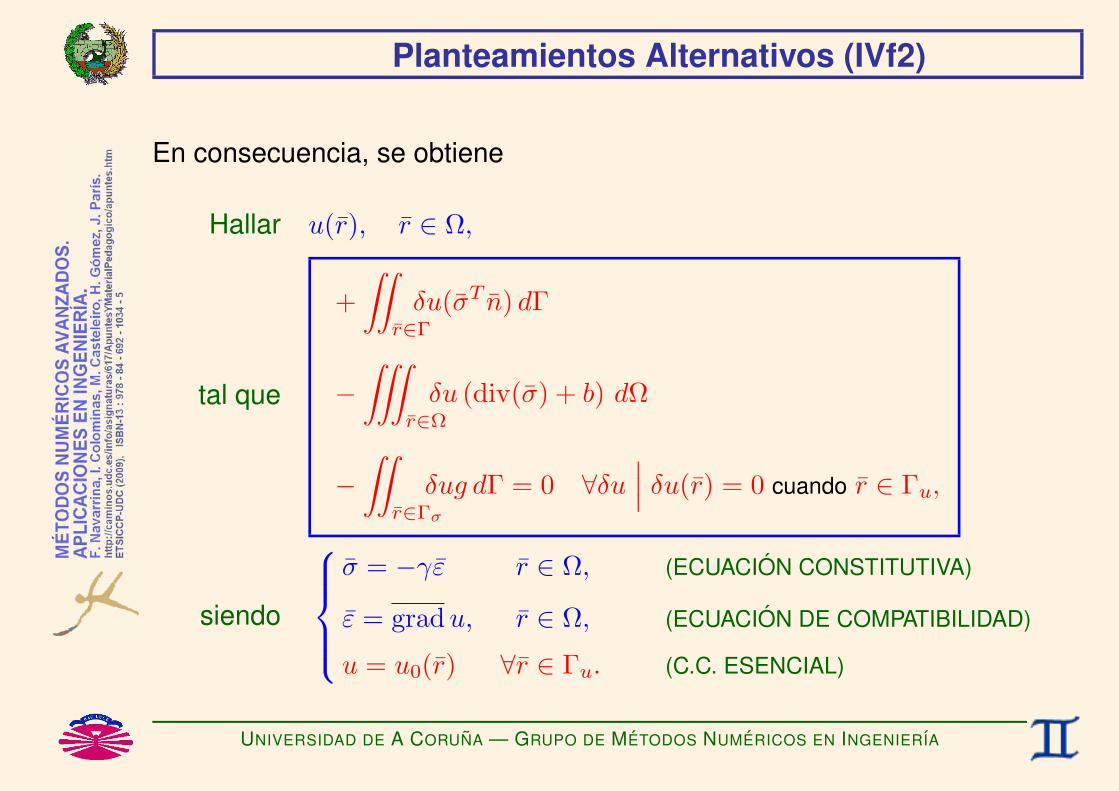
Planteamientos Alternativos (IVf2)
En consecuencia, se obtiene
Hallar u(r), r ∈ Ω,
tal que
+∫∫r∈Γ
δu(σT n) dΓ
−∫∫∫
r∈Ω
δu (div(σ) + b) dΩ
−∫∫r∈Γσ
δug dΓ = 0 ∀δu∣∣∣ δu(r) = 0 cuando r ∈ Γu,
siendo
σ = −γε r ∈ Ω, (ECUACION CONSTITUTIVA)
ε = gradu, r ∈ Ω, (ECUACION DE COMPATIBILIDAD)
u = u0(r) ∀r ∈ Γu. (C.C. ESENCIAL)
UNIVERSIDAD DE A CORUNA — GRUPO DE METODOS NUMERICOS EN INGENIERIA

Planteamientos Alternativos (IVg)
. . . o lo que es lo mismo,Hallar u(r), r ∈ Ω,
tal que
∫∫∫r∈Ω
ω(r)R(r) dΩ +∫∫r∈Γσ
ω(r)RΓ(r) dΓ = 0,
ω(r) = δu(r), ∀δu∣∣∣ δu(r) = 0 cuando r ∈ Γu,
(*)
siendo
R(r) = div(σ) + b r ∈Ω, (EC. DE EQUILIBRIO)
σ = −γε r ∈ Ω, (EC. CONSTITUTIVA)
ε = gradu r ∈ Ω, (EC. DE COMPATIBILIDAD)
RΓ(r) = −σT n+ g(r) r ∈ Γσ, (C.C. NATURAL)
u = u0(r) ∀r ∈ Γu. (C.C. ESENCIAL)
(*) Que es un planteamiento en residuos ponderados equivalente al problema original.
UNIVERSIDAD DE A CORUNA — GRUPO DE METODOS NUMERICOS EN INGENIERIA

Residuos Ponderados: Forma Debil (I)
PLAN DE TRABAJO
UNIVERSIDAD DE A CORUNA — GRUPO DE METODOS NUMERICOS EN INGENIERIA

Residuos Ponderados: Forma Debil (II)
RESIDUOS PONDERADOS (Weighted Residuals)
Hallar u(r), r ∈ Ω,
tal que∫∫∫
r∈Ω
ω(r)R(r) dΩ +∫∫r∈Γσ
ω(r)RΓ(r) dΓ = 0 ∀ω(r)
siendo
R(r) = div(σ) + b r ∈Ω, (EC. DE EQUILIBRIO)
σ = −γε r ∈ Ω, (EC. CONSTITUTIVA)
ε = gradu r ∈ Ω, (EC. DE COMPATIBILIDAD)
RΓ(r) = −σT n+ g(r) r ∈ Γσ, (C.C. NATURAL)
u = u0(r) ∀r ∈ Γu. (C.C. ESENCIAL)
UNIVERSIDAD DE A CORUNA — GRUPO DE METODOS NUMERICOS EN INGENIERIA

Residuos Ponderados: Forma Debil (III)
Observamos que
♣ En el enunciado anterior las funciones de prueba u(r) se derivan dosveces, mientras que las funciones de test ω(r) no se derivan.
♠ Si tenemos una aproximacion a la solucion uh(r) ≈ u(r) que no sea dosveces derivable, el enunciado anterior no permite comprobar la bondadde la aproximacion.
♥ Si pudiesemos reducir el orden de derivacion de u(r) podrıamos intentarobtener aproximaciones con menores requisitos de continuidad (porejemplo, poligonales a trozos)
Aplicaremos EL TEOREMA DE LA DIVERGENCIA con el fin de reducirel orden de derivacion de u(r) aunque sea a costa de aumentar el ordende derivacion de ω(r).
UNIVERSIDAD DE A CORUNA — GRUPO DE METODOS NUMERICOS EN INGENIERIA

Residuos Ponderados: Forma Debil (IVa1)
Operando,
div(ωσ) = gradT(ω)σ + ω div(σ).
Y, por tanto,ZZZr∈Ω
div(ωσ) dΩ =
ZZZr∈Ω
gradT(ω)σ dΩ +
ZZZr∈Ω
ω div(σ) dΩ.
TEOREMA DE LA DIVERGENCIAZZZr∈Ω
div(ωσ) dΩ =
ZZr∈Γ
(ωσ)Tn dΓ
=
ZZr∈Γ
ω(σTn) dΓ.
UNIVERSIDAD DE A CORUNA — GRUPO DE METODOS NUMERICOS EN INGENIERIA

Residuos Ponderados: Forma Debil (IVa2)
Luego, ∫∫∫r∈Ω
ωR dΩ =∫∫∫
r∈Ω
ω (div(σ) + b) dΩ
=∫∫r∈Γ
ω(σT n) dΓ
−∫∫∫
r∈Ω
gradT(ω)σ dΩ +
∫∫∫r∈Ω
ωb dΩ
=∫∫r∈Γσ
ω(σT n) dΓ +∫∫r∈Γu
ω(σT n) dΓ
−∫∫∫
r∈Ω
gradT(ω)σ dΩ +
∫∫∫r∈Ω
ωb dΩ.
UNIVERSIDAD DE A CORUNA — GRUPO DE METODOS NUMERICOS EN INGENIERIA

Residuos Ponderados: Forma Debil (IVb)
En consecuencia,∫∫∫r∈Ω
ωR dΩ +∫∫r∈Γσ
ωRΓ =∫∫r∈Γσ
ω(σT n) dΓ +∫∫r∈Γu
ω(σT n) dΓ
−∫∫∫
r∈Ω
gradT(ω)σ dΩ +
∫∫∫r∈Ω
ωb dΩ
+∫∫r∈Γσ
ω(−σT n+ g
)dΓ
=−∫∫∫
r∈Ω
gradT(ω)σ dΩ +
∫∫∫r∈Ω
ωb dΩ
+∫∫r∈Γσ
ωg dΓ +∫∫r∈Γu
ω(σT n
)︸ ︷︷ ︸gR
dΓ,
lo que nos conduce a la forma debil. . .
UNIVERSIDAD DE A CORUNA — GRUPO DE METODOS NUMERICOS EN INGENIERIA

Residuos Ponderados: Forma Debil (V)
FORMA DEBIL (Weak Form)
Hallar u(r) ∈ Hu,[y la reaccion g
R= σT n
]
tal que
∫∫∫r∈Ω
gradT(ω)σ dΩ =
∫∫∫r∈Ω
ωb dΩ +∫∫r∈Γσ
ωg dΓ
+∫∫r∈Γu
ωgRdΓ ∀ω(r) ∈ Hω
siendo
σ = −γε r ∈ Ω, (EC. CONSTITUTIVA)
ε = gradu r ∈ Ω, (EC. DE COMPATIBILIDAD)
u = u0(r) ∀r ∈ Γu. (C.C. ESENCIAL)
donde gR
= σT n es la REACCION que se produce en Γu al forzar el valor dela condicion de contorno esencial.
UNIVERSIDAD DE A CORUNA — GRUPO DE METODOS NUMERICOS EN INGENIERIA

Residuos Ponderados: Forma Debil (VI)
Observamos que
♦ La forma anterior es DEBIL por doble motivo, ya que ademas de loanteriormente expuesto permite comprobar la bondad deaproximaciones uh(r) ≈ u(r) que sean una vez derivables (en vez dedos veces derivables, como exige la forma fuerte del problema).
♥ La condicion de contorno natural se introduce en la formulacionmediante el termino
∫∫r∈Γσ
ωg dΓ.
♣ Cuando g = 0 se impone una condicion de contorno que establece que σT n = 0
en Γσ, pero el terminoZZ
r∈Γσ
ωg dΓ desaparece, por lo que la condicion de contorno
parece satisfacerse de forma “natural”. De ahı el nombre.
UNIVERSIDAD DE A CORUNA — GRUPO DE METODOS NUMERICOS EN INGENIERIA
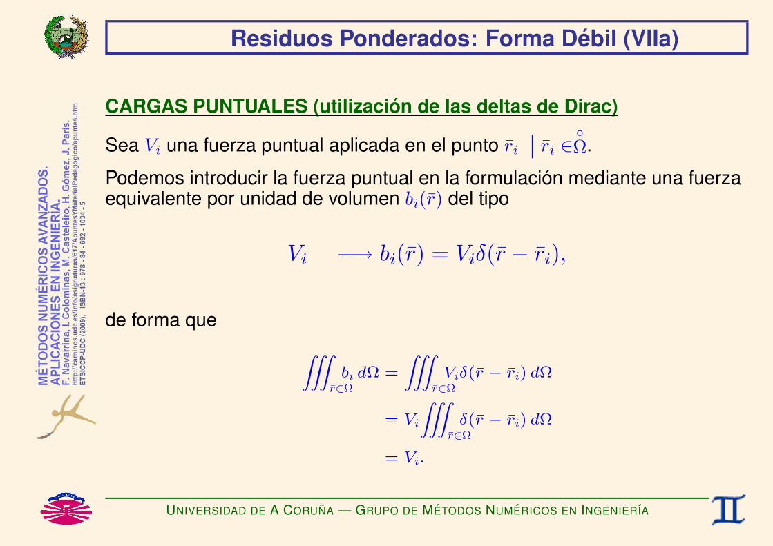
Residuos Ponderados: Forma Debil (VIIa)
CARGAS PUNTUALES (utilizacion de las deltas de Dirac)
Sea Vi una fuerza puntual aplicada en el punto ri∣∣ ri ∈ Ω.
Podemos introducir la fuerza puntual en la formulacion mediante una fuerzaequivalente por unidad de volumen bi(r) del tipo
Vi −→ bi(r) = Viδ(r − ri),
de forma que ZZZr∈Ω
bi dΩ =
ZZZr∈Ω
Viδ(r − ri) dΩ
= Vi
ZZZr∈Ω
δ(r − ri) dΩ
= Vi.
UNIVERSIDAD DE A CORUNA — GRUPO DE METODOS NUMERICOS EN INGENIERIA

Residuos Ponderados: Forma Debil (VIIb)
Al introducir bi(r) en la forma debil obtenemos∫∫∫r∈Ω
ωbi dΩ =∫∫∫
r∈Ω
ωViδ(r − ri) dΩ
= Vi
∫∫∫r∈Ω
ωδ(r − ri) dΩ
= Viω(ri),
que es un termino del mismo tipo de los que se obtuvieron anteriormente enproblemas 1D.
De la misma forma pueden introducirse cargas concentradas sobre unasuperficie, o sobre una lınea.
UNIVERSIDAD DE A CORUNA — GRUPO DE METODOS NUMERICOS EN INGENIERIA

Residuos Ponderados: Forma Debil (VIIIa)
EL PRINCIPIO DE LOS TRABAJOS VIRTUALES
♥ Si interpretamos la funcion de test ω(r) como un desplazamiento virtualcompatible con las condiciones de contorno esenciales (es decir comouna modificacion de la solucion u(r) que no incumpla las condiciones decontorno esenciales), e interpretamos su derivada como unadeformacion virtual, podemos escribir
ω(r) = δu(r) con δu(r) = 0 ∀r ∈ Γu, δε(r) =∂ω
∂x
y obtenemos el PRINCIPIO DE LOS TRABAJOS VIRTUALES∫∫∫r∈Ω
δεT σ dΩ =∫∫∫
r∈Ω
δub dΩ +∫∫r∈Γσ
δug dΓ
∀δu∣∣∣ δu(r) = 0 cuando r ∈ Γu.
UNIVERSIDAD DE A CORUNA — GRUPO DE METODOS NUMERICOS EN INGENIERIA
Residuos Ponderados: Forma Debil (VIIIb)
♣ Por tanto, el PRINCIPIO DE LOS TRABAJOS VIRTUALES es unaforma debil de las ecuaciones de equilibrio (no de las ecuacionesconstitutivas ni de las de compatibilidad) y de las condiciones decontorno naturales (no de las condiciones de contorno esenciales).
♥ El METODO DE RESIDUOS PONDERADOS permite obtener una formadebil del problema aunque no se conozca el enunciado especıfico delPTV para el problema que se esta resolviendo (por ejemplo, ¿quesignifica y como se escribe el principio de los trabajos virtuales enproblemas de difusion de contaminantes?)
♦ En el caso que nos ocupa, esta forma debil equivale al planteamientovariacional de mınima energıa, por lo que las soluciones numericas queproporcionara el metodo de Galerkin seran optimas. Esto no tiene porque ser cierto en otros casos (problemas de conveccion-difusion,dinamica de fluidos, etc.).
UNIVERSIDAD DE A CORUNA — GRUPO DE METODOS NUMERICOS EN INGENIERIA
Residuos Ponderados: Forma Debil (VIIIc)
♣ La forma clasica del bf PTV tambien es valida para ecuacionesconstitutivas no lineales y para ecuaciones de compatibilidad mascomplicadas siempre y cuando la ecuacion de equilibrio sea la expuesta.En todo caso, hay que interpretar correctamente el enunciado y tener encuenta que la expresion de la deformacion virtual es la correspondienteal gradiente.
UNIVERSIDAD DE A CORUNA — GRUPO DE METODOS NUMERICOS EN INGENIERIA
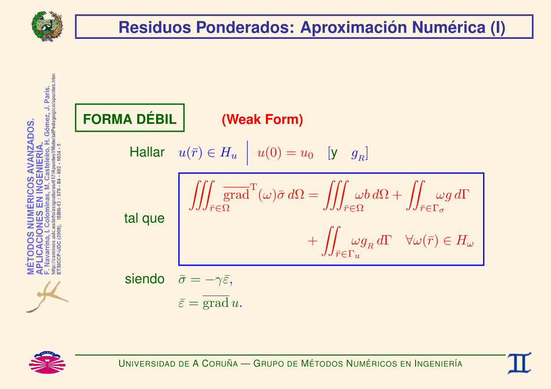
Residuos Ponderados: Aproximacion Numerica (I)
FORMA DEBIL (Weak Form)
Hallar u(r) ∈ Hu
∣∣∣ u(0) = u0 [y gR]
tal que
∫∫∫r∈Ω
gradT(ω)σ dΩ =
∫∫∫r∈Ω
ωb dΩ +∫∫r∈Γσ
ωg dΓ
+∫∫r∈Γu
ωgRdΓ ∀ω(r) ∈ Hω
siendo σ = −γε,
ε = gradu.
UNIVERSIDAD DE A CORUNA — GRUPO DE METODOS NUMERICOS EN INGENIERIA

Residuos Ponderados: Aproximacion Numerica (IIa)
FUNCIONES DE PRUEBA (Trial Functions)
Sea la base de funciones de prueba φi(r)i=1,...,ν.
Dada la aproximacion inicial ψ(r), buscamos una mejor aproximacion
u(r) ≈ uh(r) = ψ(r) +ν∑i=1
αiφi(r), uh(r) ∈ Hhu ⊂ Hu,
u(r) ≈ uh(r) = ψ(r) + ΦT (r) α, con Φ(r) =
φ1(r)...φν(r)
, α =
α1...αν
.
Las correspondientes aproximaciones de ε(r) y de σ(r) seran
ε(r) ≈ εh(r) = gradψ +
νXi=1
αi gradφi, σ(r) ≈ σh(r) = −γεh(r),
ε(r) ≈ εh(r) = gradψ + grad Φ
Tα, σ(r) ≈ σ
h(r) = −γεh(r).
Y [si interesa] podemos buscar una aproximacion de la reaccion gR≈ gh
R.
UNIVERSIDAD DE A CORUNA — GRUPO DE METODOS NUMERICOS EN INGENIERIA

Residuos Ponderados: Aproximacion Numerica (IIb)
En general no sera posible que uh(r) = u(r) ∀r ∈ Ω (*), por lo que
uh(r) 6= u(r)
m
no es posible que
∫∫∫r∈Ω
gradT(ω)σh dΩ =
∫∫∫r∈Ω
ωb dΩ
+∫∫r∈Γσ
ωg dΓ +∫∫r∈Γu
ωghRdΓ ∀ω(r) ∈ Hω.
(*) Salvo que u(r)− ψ(r) este contenido en el subespacio generado por las funciones de prueba.
UNIVERSIDAD DE A CORUNA — GRUPO DE METODOS NUMERICOS EN INGENIERIA
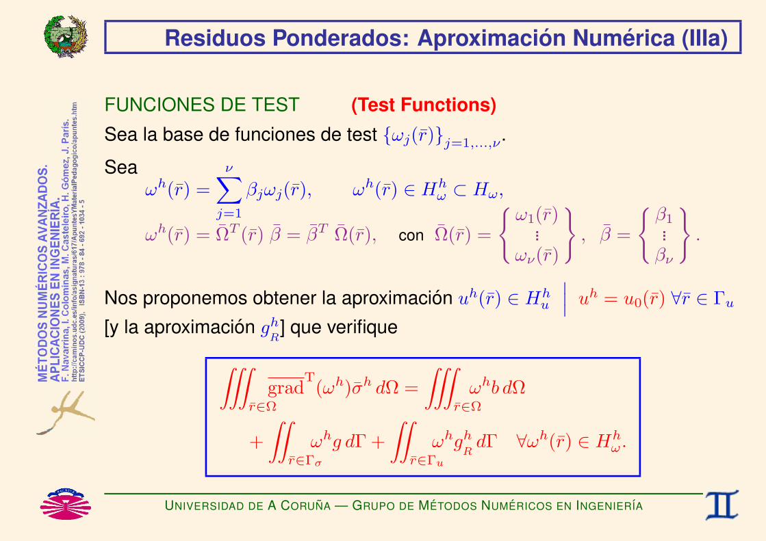
Residuos Ponderados: Aproximacion Numerica (IIIa)
FUNCIONES DE TEST (Test Functions)Sea la base de funciones de test ωj(r)j=1,...,ν.
Seaωh(r) =
ν∑j=1
βjωj(r), ωh(r) ∈ Hhω ⊂ Hω,
ωh(r) = ΩT (r) β = βT Ω(r), con Ω(r) =
ω1(r)...ων(r)
, β =
β1...βν
.
Nos proponemos obtener la aproximacion uh(r) ∈ Hhu
∣∣∣ uh = u0(r) ∀r ∈ Γu[y la aproximacion gh
R] que verifique∫∫∫
r∈Ω
gradT(ωh)σh dΩ =
∫∫∫r∈Ω
ωhb dΩ
+∫∫r∈Γσ
ωhg dΓ +∫∫r∈Γu
ωhghRdΓ ∀ωh(r) ∈ Hh
ω.
UNIVERSIDAD DE A CORUNA — GRUPO DE METODOS NUMERICOS EN INGENIERIA

Residuos Ponderados: Aproximacion Numerica (IIIb)
PeroZZZr∈Ω
gradT(ω
h)σ
hdΩ−
ZZZr∈Ω
ωhb dΩ−
ZZr∈Γσ
ωhg dΓ−
ZZr∈Γu
ωhgh
RdΓ = 0 ∀ωh(r) ∈ Hh
ω
mνXj=1
βj
„ZZZr∈Ω
gradT(ωj)σ
hdΩ−
ZZZr∈Ω
ωjb dΩ−ZZ
r∈Γσ
ωjg dΓ−ZZ
r∈Γu
ωjgh
RdΓ
«= 0 ∀ βj
βT
„ZZZr∈Ω
gradT(Ω)σ
hdΩ−
ZZZr∈Ω
Ωb dΩ−ZZ
r∈Γσ
Ωg dΓ−ZZ
r∈Γu
Ωgh
RdΓ
«= 0 ∀β
mZZZr∈Ω
gradT(ωj)σ
hdΩ =
ZZZr∈Ω
ωjb dΩ +
ZZr∈Γσ
ωjg dΓ +
ZZr∈Γu
ωjgh
RdΓ, j=1,...,νZZZ
r∈Ω
gradT(Ω)σ
hdΩ =
ZZZr∈Ω
Ωb dΩ +
ZZr∈Γσ
Ωg dΓ +
ZZr∈Γu
Ωgh
RdΓ.
UNIVERSIDAD DE A CORUNA — GRUPO DE METODOS NUMERICOS EN INGENIERIA

Residuos Ponderados: Aproximacion Numerica (IVa)
Por tanto,
−ZZZ
r∈Ωgrad
T(ωj)γ
gradψ +
νXi=1
αi gradφi
!dΩ =
ZZZr∈Ωωjb dΩ +
ZZr∈Γσωjg dΓ +
ZZr∈Γuωjg
h
RdΓ, j=1,...,ν
−ZZZ
r∈Ωgrad
T(Ω)γ
“gradψ + grad Φ
Tα”dΩ =
ZZZr∈ΩΩb dΩ +
ZZr∈ΓσΩg dΓ +
ZZr∈ΓσΩg
h
RdΓ
m
νXi=1
kjiz | „−ZZZ
r∈Ωgrad
T(ωj)γ gradφi dΩ
«αi =
fjz | ZZZr∈Ωgrad
T(ωj)γ gradψ dΩ +
ZZZr∈Ωωjb dΩ +
ZZr∈Γσωjg dΓ +
ZZr∈Γuωjg
h
RdΓ, j=1,...,ν
Kez | „−ZZZ
r∈Ωgrad
T(Ω)γ grad Φ
TdΩ
«α =
fz | ZZZr∈Ωgrad
T(Ω)γ gradψ dΩ +
ZZZr∈ΩΩb dΩ +
ZZr∈ΓσΩg dΓ +
ZZr∈ΓuΩg
h
RdΓ
m
νXi=1
kjiαi = fj +
ZZr∈Γuωjg
h
RdΓ j=1,...,ν ⇐⇒ Ke α = f +
ZZr∈ΓuΩg
h
RdΓ.
UNIVERSIDAD DE A CORUNA — GRUPO DE METODOS NUMERICOS EN INGENIERIA

Residuos Ponderados: Aproximacion Numerica (IVb)
Luego el problema de equilibrio original ha sido sustituido por el sistema(de orden ν, con la incognita adicional gh
R(r), r ∈ Γu)
K˜ α = f +∫∫r∈Γu
Ω(r)ghR(r) dΓ,
con la condicion adicional uh = u0(r) ∀r ∈ Γu, esto es
ΦT (r) α = u0(r)− ψ(r) ∀r ∈ Γu.
♠ ¡AHORA NO ES TRIVIAL IMPONER LAS CONDICIONES DECONTORNO ESENCIALES!Ya que deben cumplirse ∀r ∈ Γu.
UNIVERSIDAD DE A CORUNA — GRUPO DE METODOS NUMERICOS EN INGENIERIA

Residuos Ponderados: Aproximacion Numerica (IVc)
Podemos solventar el problema de las condiciones de contornoesenciales. . .
♣ mediante RESIDUOS PONDERADOS,
♣ eligiendo adecuadamente la aproximacion inicial ψ(r) y las funciones deprueba Φ(r), o
♥ mediante ELEMENTOS FINITOS de forma trivial.
UNIVERSIDAD DE A CORUNA — GRUPO DE METODOS NUMERICOS EN INGENIERIA
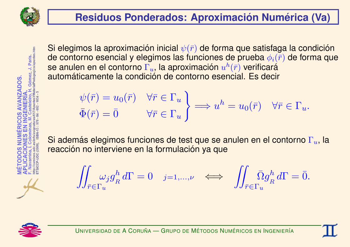
Residuos Ponderados: Aproximacion Numerica (Va)
Si elegimos la aproximacion inicial ψ(r) de forma que satisfaga la condicionde contorno esencial y elegimos las funciones de prueba φi(r) de forma quese anulen en el contorno Γu, la aproximacion uh(r) verificaraautomaticamente la condicion de contorno esencial. Es decir
ψ(r) = u0(r) ∀r ∈ ΓuΦ(r) = 0 ∀r ∈ Γu
=⇒ uh = u0(r) ∀r ∈ Γu.
Si ademas elegimos funciones de test que se anulen en el contorno Γu, lareaccion no interviene en la formulacion ya que∫∫
r∈Γu
ωjghRdΓ = 0 j=1,...,ν ⇐⇒
∫∫r∈Γu
ΩghRdΓ = 0.
UNIVERSIDAD DE A CORUNA — GRUPO DE METODOS NUMERICOS EN INGENIERIA

Residuos Ponderados: Aproximacion Numerica (Vb)
Por tanto, el sistema de ecuaciones que hay que resolver puede escribirseen la forma
K˜ α = f ,
siendo
Ke = [kji]i=1,...,νj=1,...,ν
, kji =
ZZZr∈Ω
gradT(ωj)γ gradφi dΩ
Ke =
ZZZr∈Ω
gradT(Ω)γ grad ΦT dΩ
f = fjj=1,...,ν , fj = −ZZZ
r∈Ω
gradT(ωj)γ gradψ dΩ +
ZZZr∈Ω
ωjb dΩ +
ZZr∈Γσ
ωjg dΓ
f = −ZZZ
r∈Ω
gradT(Ω)γ gradψ dΩ +
ZZZr∈Ω
Ωb dΩ +
ZZr∈Γσ
Ωg dΓ.
UNIVERSIDAD DE A CORUNA — GRUPO DE METODOS NUMERICOS EN INGENIERIA

Residuos Ponderados: Aproximacion Numerica (VI)
Una vez resuelto el sistema obtendremos la aproximacion a la solucion
uh(r) = ψ(r) +ν∑i=0
αiφi(r) ⇐⇒ uh(r) = ψ(r) + ΦT (r) α.
εh(r) = gradψ +ν∑i=1
αi gradφi ⇐⇒ εh(r) = gradψ + gradT(Φ) α
σh(r) = −γεh(r) ⇐⇒ σh(r) = −γεh(r).
UNIVERSIDAD DE A CORUNA — GRUPO DE METODOS NUMERICOS EN INGENIERIA

Residuos Ponderados: Error de Aproximacion (I)
METODOS DE PROYECCION
Los METODOS DE RESIDUOS PONDERADOS tambien se denominan ası,ya que siendo
u(r) la solucion exacta, con ε(r) = gradu, σ(r) = −γε(r)
uh(r) la solucion aproximada, con εh(r) = graduh, σh(r) = −γεh(r)
se verificaZZZr∈Ω
gradT(ωh)σ dΩ =
ZZZr∈Ωωhb dΩ +
ZZr∈Γσ
ωhg dΓ +
ZZr∈Γu
ωhgRdΓ ∀ωh(r) ∈ Hh
ω
ZZZr∈Ω
gradT(ωh)σhdΩ =
ZZZr∈Ωωhb dΩ +
ZZr∈Γσ
ωhg dΓ +
ZZr∈Γu
ωhgh
RdΓ ∀ωh(r) ∈ Hh
ω
9>>>>=>>>>; =⇒
=⇒ZZZ
r∈Ωgrad
T(ωh)(σ − σ
h) dΩ =
ZZr∈Γu
ωh(gR− g
h
R) dΓ ∀ωh(r) ∈ Hh
ω.
UNIVERSIDAD DE A CORUNA — GRUPO DE METODOS NUMERICOS EN INGENIERIA

Residuos Ponderados: Error de Aproximacion (II)
La ecuacion anterior demuestra que (normalmente) la integral de lasreacciones se calcula exactamente, ya que si la funcion constantepertenece al espacio de las funciones de test (lo que normalmente se exigey se conoce como PARTICION DE LA UNIDAD) entonces
ωh(r) = 1 =⇒∫∫r∈Γu
gRdΓ =
∫∫r∈Γu
ghRdΓ .
Si las funciones de test ωh se anulan en Γu se cumpleZZZr∈Ω
gradT(ω
h)γ grad(u− u
h) dΩ = 0 ∀ωh(r) ∈ Hh
ω, ωh(r) = 0 en Γu.
Luego (normalmente), la solucion aproximada uh(r) verifica
⟨ωh, u− uh
⟩= 0 ∀ωh(r) ∈ Hh
ω, con 〈v, e〉 =∫∫∫
r∈Ω
gradT(v)γ grad(e) dΩ.
UNIVERSIDAD DE A CORUNA — GRUPO DE METODOS NUMERICOS EN INGENIERIA

Residuos Ponderados: Error de Aproximacion (III)
Por tanto, la solucion aproximada uh(r) es
la PROYECCION de la solucion exacta u(r)
sobre el subespacio Hhu de las funciones de prueba uh(r)
segun la normal al subespacio Hhω de las funciones de test ωh(r).
UNIVERSIDAD DE A CORUNA — GRUPO DE METODOS NUMERICOS EN INGENIERIA

Eleccion de las Funciones de Test
Algunas posibilidades. . .
1) METODO DE COLOCACION PUNTUAL
ωj(r) = δ(r − rj), j=1,...,ν con rj∈Ω, ri 6=rj ∀i6=j. (*)
=⇒ No se puede utilizar en este caso, porque la delta no es derivable.Si se aplica a la forma original de RP conduce a DIFERENCIAS FINITAS.
2) METODO DE COLOCACION POR SUBDOMINIOS
ωj(r) = 1, si r ∈ Ωj,
0, en caso contrario, j=1,...,ν conν⋃j=1
Ωj = Ω,ν⋂j=1
Ωj= ∅.
=⇒ Conduce a VOLUMENES FINITOS.
3) METODO DE BUBNOV-GALERKIN
ωj(r) = φj(r), j=1,...,ν ⇐⇒ Hhω = Hh
u .
(*) Si rj = a o rj = b es preciso redefinir adecuadamente la δ.
UNIVERSIDAD DE A CORUNA — GRUPO DE METODOS NUMERICOS EN INGENIERIA

Metodo de Bubnov-Galerkin (Ia)
PONDERACION DE BUBNOV–GALERKIN
Si se eligen como funciones de test las funciones de prueba, esto es
Hhω = Hh
u
mωj(r) = φj(r), j=0,...,ν ⇐⇒ Ω(r) = Φ(r),
se obtiene
Ke = [kji]i=1,...,νj=1,...,ν
, kji =
ZZZr∈Ω
gradT(φj)γ gradφi dΩ
Ke =
ZZZr∈Ω
gradT(Φ)γ grad ΦT dΩ
f = fjj=1,...,ν , fj = −ZZZ
r∈Ω
gradT(φj)γ gradψ dΩ +
ZZZr∈Ω
φjb dΩ +
ZZr∈Γσ
φjg dΓ
f = −ZZZ
r∈Ω
gradT(Φ)γ gradψ dΩ +
ZZZr∈Ω
Φb dΩ +
ZZr∈Γσ
Φg dΓ.
UNIVERSIDAD DE A CORUNA — GRUPO DE METODOS NUMERICOS EN INGENIERIA

Metodo de Bubnov-Galerkin (Ib)
Como ya hemos visto, si elegimos la aproximacion inicial ψ(r) de forma quesatisfaga la condicion de contorno esencial y elegimos las funciones deprueba φi(r) de forma que se anulen en el contorno Γu, la aproximacionuh(r) verificara automaticamente la condicion de contorno esencial. Es decir
ψ(r) = u0(r) ∀r ∈ ΓuΦ(r) = 0 ∀r ∈ Γu
=⇒ uh = u0(r) ∀r ∈ Γu.
Como estamos utilizando una ponderacion de Bubnov–Galerkin,automaticamente las funciones de test se anularan en el contorno Γu, y lareaccion no interviene en la formulacion ya que∫∫
r∈Γu
φjghRdΓ = 0 j=1,...,ν ⇐⇒
∫∫r∈Γu
ΦghRdΓ = 0.
UNIVERSIDAD DE A CORUNA — GRUPO DE METODOS NUMERICOS EN INGENIERIA

Metodo de Bubnov-Galerkin (Ic)
Por tanto, el sistema de ecuaciones que hay que resolver puede escribirseen la forma
K˜ α = f ,
siendo
Ke =
2666666664
ZZZr∈Ω
gradT(φ1)γ gradφ1 dΩ
ZZZr∈Ω
gradT(φ1)γ gradφ2 dΩ . . .
ZZZr∈Ω
gradT(φ1)γ gradφν dΩZZZ
r∈Ωgrad
T(φ2)γ gradφ1 dΩ
ZZZr∈Ω
gradT(φ2)γ gradφ2 dΩ . . .
ZZZr∈Ω
gradT(φ2)γ gradφν dΩ
... ... ...ZZZr∈Ω
gradT(φν)γ gradφ1 dΩ
ZZZr∈Ω
gradT(φν)γ gradφ2 dΩ . . .
ZZZr∈Ω
gradT(φν)γ gradφν dΩ
3777777775
f =
8>>>>>>>><>>>>>>>>:
−ZZZ
r∈Ωgrad
T(φ1)γ gradψ dΩ +
ZZZr∈Ωφ1b dΩ +
ZZr∈Γσ
φ1g dΓ
−ZZZ
r∈Ωgrad
T(φ2)γ gradψ dΩ +
ZZZr∈Ωφ2b dΩ +
ZZr∈Γσ
φ2g dΓ
...−ZZZ
r∈Ωgrad
T(φν)γ gradψ dΩ +
ZZZr∈Ωφνb dΩ +
ZZr∈Γσ
φνg dΓ
9>>>>>>>>=>>>>>>>>;.
UNIVERSIDAD DE A CORUNA — GRUPO DE METODOS NUMERICOS EN INGENIERIA

Metodo de Bubnov-Galerkin (II)
La solucion aproximada uh(r) verifica∫∫∫r∈Ω
gradT(φj)σh dΩ−
∫∫∫r∈Ω
φjb dΩ−∫∫r∈Γσ
φjg dΓ = 0
⇓
∂E
∂αj= 0, siendo E(α1, α2, . . . , αν) = E [uh],
por lo que se realiza un AJUSTE DE MINIMA ENERGIA.
UNIVERSIDAD DE A CORUNA — GRUPO DE METODOS NUMERICOS EN INGENIERIA

Metodo de Bubnov-Galerkin (IIIa)
La matriz K˜ del metodo de Galerkin es. . .
♥ SIMETRICAK˜ = K˜ T
♥ SEMIDEFINIDA POSITIVA
ηTK˜ η ≥ 0 ∀η 6= 0
♥ DEFINIDA POSITIVA
ηTK˜ η > 0 ∀η 6= 0 (*)
(*) Si la base de funciones de prueba ha sido correctamente elegida.
UNIVERSIDAD DE A CORUNA — GRUPO DE METODOS NUMERICOS EN INGENIERIA

Metodo de Bubnov-Galerkin (IIIb)
K˜ es SIMETRICA, ya que
kji =
ZZZr∈Ω
grad(φj)γ grad(φi) dΩ =
ZZZr∈Ω
grad(φi)γ grad(φj) dΩ = kij
m
Ke =
ZZZr∈Ω
grad(Φ)γ grad(ΦT) dΩ =
ZZZr∈Ω
“grad(Φ)γ grad(Φ
T)”T
dΩ = Ke T .
UNIVERSIDAD DE A CORUNA — GRUPO DE METODOS NUMERICOS EN INGENIERIA

Metodo de Bubnov-Galerkin (IIIc)
K˜ es SEMIDEFINIDA POSITIVA, ya queνXj=1
νXi=1
ηjkjiηi =νXj=1
νXi=1
ηj
„ZZZr∈Ω
grad(φj)γ grad(φi) dΩ
«ηi
=
ZZZr∈Ω
0@ νXj=1
ηj grad(φj)
1A| z
g(r)
γ
νXi=1
ηi grad(φi)
!| z
g(r)
dΩ
=
ZZZr∈Ω
νXi=1
ηi grad(φi)
!2
γ dΩ ≥ 0 ∀η = ηii=1,...,ν 6= 0.
mηTKe η = η
T„ZZZ
r∈Ωgrad(Φ)γ grad(Φ
T) dΩ
«η
=
ZZZr∈Ω
grad(ΦTη)| z
g(r)
γ grad(ΦTη)| z
g(r)
dΩ
=
ZZZr∈Ω
“grad(Φ
Tη)”2γ dΩ ≥ 0 ∀η 6= 0.
UNIVERSIDAD DE A CORUNA — GRUPO DE METODOS NUMERICOS EN INGENIERIA

Metodo de Bubnov-Galerkin (IIId)
K˜ es DEFINIDA POSITIVA, ya que (vease el punto anterior)
νXj=1
νXi=1
ηjkjiηi = 0 =⇒νXi=1
ηi grad(φi) = 0 ∀r ∈ Ω =⇒ ηi = 0, i = 1, . . . , ν
m
ηTKe η = 0 =⇒ grad(Φ
Tη) = 0 ∀r ∈ Ω =⇒ η = 0.
si la base de funciones de prueba ha sido correctamente elegida (de formaque sus derivadas sean linealmente independientes).
UNIVERSIDAD DE A CORUNA — GRUPO DE METODOS NUMERICOS EN INGENIERIA

Metodo de Bubnov-Galerkin (IVa)
ESTIMACION DEL ERROR
Sabemos que la solucion aproximada uh(r) verifica
Dωh, u− u
hE
= 0 ∀ωh(r) ∈ Hhω = H
hu, con 〈v, e〉 =
ZZZr∈Ω
gradT(v)γ grad(e) dΩ.
El producto escalar verifica la desigualdad de Cauchy
〈v, e〉 ≤ ‖v‖ ‖e‖ , con la norma ‖e‖ = 〈e, e〉12 =
sZZZr∈Ω
˛grad(e)
˛2γ dΩ.
UNIVERSIDAD DE A CORUNA — GRUPO DE METODOS NUMERICOS EN INGENIERIA

Metodo de Bubnov-Galerkin (IVb)
APROXIMACION OPTIMA
La solucion aproximada uh(r) verifica
∥∥u− uh∥∥ ≤ ∥∥u− vh
∥∥ ∀vh ∈ Hhu .
UNIVERSIDAD DE A CORUNA — GRUPO DE METODOS NUMERICOS EN INGENIERIA

Metodo de Bubnov-Galerkin (IVc)
Pues,
uh, v
h ∈ Hhu =⇒ u
h − vh ∈ Hh
u =⇒Duh − v
h, u− u
hE
= 0,
luego
‚‚‚u− uh‚‚‚2
=Du− u
h, u− u
hE
+ 0 =Du− u
h, u− u
hE
+Duh − v
h, u− u
hE
=Du− u
h+ u
h − vh, u− u
hE
=Du− v
h, u− u
hE
≤‚‚‚u− v
h‚‚‚ ‚‚‚u− u
h‚‚‚ ,
y en consecuencia ‚‚‚u− uh‚‚‚ ≤ ‚‚‚u− v
h‚‚‚ .
UNIVERSIDAD DE A CORUNA — GRUPO DE METODOS NUMERICOS EN INGENIERIA

Metodo de Bubnov-Galerkin (IVd)
ESTIMACION DEL ERROR
Utilizando funciones de prueba vh ∈ Hhu adecuadamente elegidas se
pueden obtener cotas del error u− uh a partir de la expresion∥∥u− uh∥∥ ≤ ∥∥u− vh
∥∥ .
UNIVERSIDAD DE A CORUNA — GRUPO DE METODOS NUMERICOS EN INGENIERIA

Eleccion de las Funciones de Prueba (Ia)
Algunas posibilidades. . .
1) SOPORTE GLOBAL → METODO DE RITZ
♣ Ejemplos:B No es trivial plantear ejemplos de aproximaciones de este tipo en 2D/3DB . . .
♠ Ke es LLENA → tiempo de computacion T (ν3).
♠ Ke puede ser MAL-CONDICIONADA. (*)
(*) EL numero de condicion depende de la base de funciones de prueba que se hayan elegido.
UNIVERSIDAD DE A CORUNA — GRUPO DE METODOS NUMERICOS EN INGENIERIA

Eleccion de las Funciones de Prueba (Ib)
2) SOPORTE LOCAL → METODO DE ELEMENTOS FINITOS
♣ Ejemplos:B a) Mallas de triangulos/tetraedros.B b) Mallas de cuadrilateros/prismas.B c) Mallas de elementos curvos.
♥ Se pretende que Ke sea SPARSE.
♥ Se pretende que Ke sea BIEN-CONDICIONADA.
UNIVERSIDAD DE A CORUNA — GRUPO DE METODOS NUMERICOS EN INGENIERIA

Notacion en Formas Bilineales (I)
FORMA DEBIL (Weak Form)
Hallar u(r) ∈ Hu
∣∣∣ u(0) = u0 [y gR]
tal que a(ω, u) = (ω, b) + (ω, g)σ + (ω, gR)u ∀ω(r) ∈ Hω,
siendo a(ω, u) =∫∫∫
r∈Ω
gradT(ω)γ grad(u) dΩ,
(ω, b) = −∫∫∫
r∈Ω
ωb dΩ,
(ω, g)σ = −∫∫r∈Γσ
ωg dΓ,
(ω, gR)u = −
∫∫r∈Γu
ωgRdΓ.
UNIVERSIDAD DE A CORUNA — GRUPO DE METODOS NUMERICOS EN INGENIERIA

Notacion en Formas Bilineales (IIa)
FUNCIONES DE PRUEBA (Trial Functions)
Sea la base de funciones de prueba φi(r)i=1,...,ν.
Dada la aproximacion inicial ψ(r), buscamos una mejor aproximacion
u(r) ≈ uh(r) = ψ(r) +ν∑i=1
αiφi(r), uh(r) ∈ Hhu ⊂ Hu,
u(r) ≈ uh(r) = ψ(r) + ΦT (r) α, con Φ(r) =
φ1(r)...φν(r)
, α =
α1...αν
.
Y [si interesa calcularla] podemos buscar una aproximacion de la reaccion
gR≈ gh
R.
UNIVERSIDAD DE A CORUNA — GRUPO DE METODOS NUMERICOS EN INGENIERIA

Notacion en Formas Bilineales (IIb)
En general no sera posible que uh(r) = u(r) ∀r ∈ Ω (*), por lo que
uh(r) 6= u(r)
m
no es posible que a(ω, uh) = (ω, b) + (ω, g)σ + (ω, gR)u ∀ω(r) ∈ Hω.
(*) Salvo que u(r)− ψ(r) este contenido en el subespacio generado por las funciones de prueba.
UNIVERSIDAD DE A CORUNA — GRUPO DE METODOS NUMERICOS EN INGENIERIA

Notacion en Formas Bilineales (IIIa)
FUNCIONES DE TEST (Test Functions)
Sea la base de funciones de test ωj(r)j=1,...,ν.
Sea
ωh(r) =ν∑j=1
βjωj(r), ωh(r) ∈ Hhω ⊂ Hω,
ωh(r) = ΩT (r) β = βT Ω(r), con Ω(r) =
ω1(r)...ων(r)
, β =
β1...βν
.
Nos proponemos obtener la aproximacion uh(r) ∈ Hhu
∣∣∣ uh = u0(r) ∀r ∈ Γu[y la aproximacion gh
R] que verifique
a(ωh, uh) = (ωh, b) + (ωh, g)σ + (ωh, ghR)u ∀ωh(r) ∈ Hh
ω.
UNIVERSIDAD DE A CORUNA — GRUPO DE METODOS NUMERICOS EN INGENIERIA
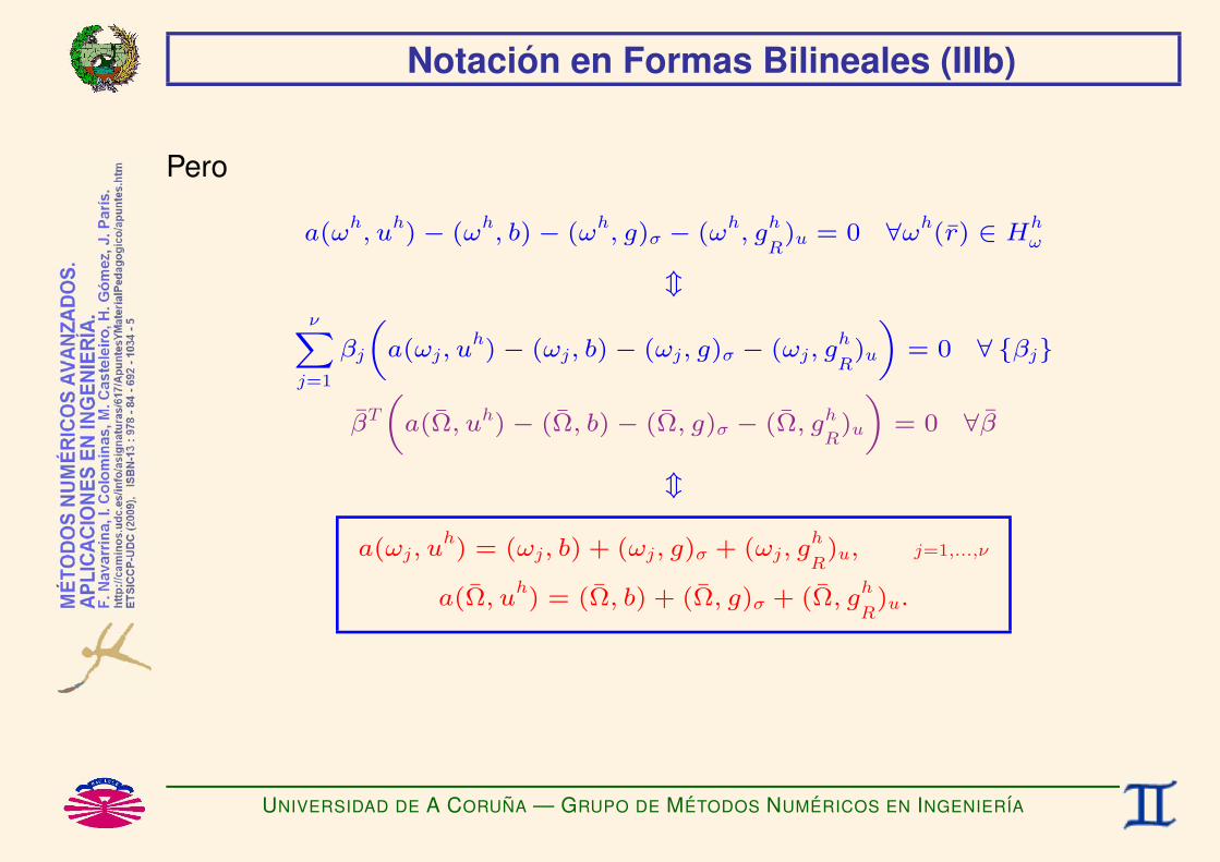
Notacion en Formas Bilineales (IIIb)
Pero
a(ωh, u
h)− (ω
h, b)− (ω
h, g)σ − (ω
h, g
h
R)u = 0 ∀ωh(r) ∈ Hh
ω
mνXj=1
βj
„a(ωj, u
h)− (ωj, b)− (ωj, g)σ − (ωj, g
h
R)u
«= 0 ∀ βj
βT„a(Ω, uh)− (Ω, b)− (Ω, g)σ − (Ω, gh
R)u
«= 0 ∀β
m
a(ωj, uh) = (ωj, b) + (ωj, g)σ + (ωj, g
h
R)u, j=1,...,ν
a(Ω, uh) = (Ω, b) + (Ω, g)σ + (Ω, g
h
R)u.
UNIVERSIDAD DE A CORUNA — GRUPO DE METODOS NUMERICOS EN INGENIERIA

Notacion en Formas Bilineales (IVa)
Por tanto,
a(ωj, ψ +
νXi=1
αiφi) = (ωj, b) + (ωj, g)σ + (ωj, gh
R)u ∀j
a(Ω, ψ + ΦT α) = (Ω, b) + (Ω, g)σ + (Ω, ghR)u
m
νXi=1
kjiz | a(ωj, φi)αi =
fjz | −a(ωj, ψ) + (ωj, b) + (ωj, g)σ +(ωj, g
h
R)u ∀j
Kez | a(Ω, Φ
T) α =
fz | −a(Ω, ψ) + (Ω, b) + (Ω, g)σ +(Ω, gh
R)u
m
νXi=1
kjiαi = fj + (ωj, gh
R)u, j=1,...,ν ⇐⇒ Ke α = f + (Ω, g
h
R)u.
UNIVERSIDAD DE A CORUNA — GRUPO DE METODOS NUMERICOS EN INGENIERIA

Notacion en Formas Bilineales (IVb)
Luego el problema de equilibrio original ha sido sustituido por el sistema(de orden ν, con la incognita adicional gh
R(r), r ∈ γu)
K˜ α = f + (Ω, ghR)u,
con la condicion adicional uh = u0(r) ∀r ∈ Γu, esto es
ΦT (r) α = u0(r)− ψ(r) ∀r ∈ Γu.
♠ ¡AHORA NO ES TRIVIAL IMPONER LAS CONDICIONES DECONTORNO ESENCIALES!Ya que deben cumplirse ∀r ∈ Γu.
UNIVERSIDAD DE A CORUNA — GRUPO DE METODOS NUMERICOS EN INGENIERIA

Notacion en Formas Bilineales (IVc)
Podemos solventar el problema de las condiciones de contornoesenciales. . .
♣ mediante RESIDUOS PONDERADOS,
♣ eligiendo adecuadamente la aproximacion inicial ψ(r) y las funciones deprueba Φ(r), o
♥ mediante ELEMENTOS FINITOS de forma trivial.
UNIVERSIDAD DE A CORUNA — GRUPO DE METODOS NUMERICOS EN INGENIERIA

Notacion en Formas Bilineales (Va)
Si elegimos la aproximacion inicial ψ(r) de forma que satisfaga la condicionde contorno esencial y elegimos las funciones de prueba φi(r) de forma quese anulen en el contorno Γu, la aproximacion uh(r) verificaraautomaticamente la condicion de contorno esencial. Es decir
ψ(r) = u0(r) ∀r ∈ ΓuΦ(r) = 0 ∀r ∈ Γu
=⇒ uh = u0(r) ∀r ∈ Γu.
Si ademas elegimos funciones de test que se anulen en el contorno Γu, lareaccion no interviene en la formulacion ya que∫∫
r∈Γu
ωjghRdΓ = 0 j=1,...,ν ⇐⇒
∫∫r∈Γu
ΩghRdΓ = 0.
UNIVERSIDAD DE A CORUNA — GRUPO DE METODOS NUMERICOS EN INGENIERIA

Notacion en Formas Bilineales (Vb)
Por tanto, el sistema de ecuaciones que hay que resolver puede escribirseen la forma
K˜ α = f ,
siendo
α = αii=1,...,ν ,Ke = [kji]i=1,...,ν
j=1,...,ν
, kji = a(ωj, φi),
Ke = a(Ω, ΦT ),
f = fjj=1,...,ν , fj = −a(ωj, ψ) + (ωj, b) + ωj(L)F,
f = −a(Ω, ψ) + (Ω, b) + Ω(L)F.
UNIVERSIDAD DE A CORUNA — GRUPO DE METODOS NUMERICOS EN INGENIERIA

Notacion en Formas Bilineales (VI)
Una vez resuelto el sistema obtendremos la aproximacion a la solucion
uh(r) = ψ(r) +ν∑i=0
αiφi(r) ⇐⇒ uh(r) = ψ(r) + ΦT (r) α.
εh(r) = gradψ +ν∑i=1
αi gradφi ⇐⇒ εh(r) = gradψ + gradT(Φ) α
σh(r) = −γεh(r) ⇐⇒ σh(r) = −γεh(r).
UNIVERSIDAD DE A CORUNA — GRUPO DE METODOS NUMERICOS EN INGENIERIA


METODO DE RESIDUOS PONDERADOS:PROBLEMAS NO ESTACIONARIOS 1D
DE TIPO PARABOLICOF. Navarrina, I. Colominas, M. Casteleiro, H. Gomez, J. Parıs
GMNI — GRUPO DE METODOS NUMERICOS EN INGENIERIA
Departamento de Metodos Matematicos y de RepresentacionEscuela Tecnica Superior de Ingenieros de Caminos, Canales y Puertos
Universidad de A Coruna, Espana
e-mail: [email protected] web: http://caminos.udc.es/gmni
UNIVERSIDAD DE A CORUNA — GRUPO DE METODOS NUMERICOS EN INGENIERIA

INDICE
I Problema Conceptual
I Residuos Ponderados: Forma Debil
I Residuos Ponderados: Aproximacion Numerica
I Metodo de Bubnov-Galerkin
UNIVERSIDAD DE A CORUNA — GRUPO DE METODOS NUMERICOS EN INGENIERIA

Problema Conceptual (I)
Sea el problema de equilibrio 1D:
UNIVERSIDAD DE A CORUNA — GRUPO DE METODOS NUMERICOS EN INGENIERIA

Problema Conceptual (II)
Modelo Matematico Lineal:
Dados A(x), b(x, t), E(x) = −γ(x), ρ, cE, u0(t), F (t), uI(x)
Hallar u(x, t), σ(x, t), x ∈ [0, L] t ≥ 0, que verifican
∂
∂x(Aσ) +A
(b+ ρcE
∂u
∂t
)= 0 (EC. DE EQUILIBRIO)
σ = Eε, (EC. CONSTITUTIVA)
ε =∂u
∂x, (EC. DE COMPATIBILIDAD)
−A(L)σ(L, t) + F (t) = 0 ∀t > 0, (C.C. NATURAL)
u(0, t) = u0(t) ∀t > 0, (C.C. ESENCIAL)
u(x, 0) = uI(x) ∀x ∈ [0, L]. (C. INICIAL)
Donde. . .
UNIVERSIDAD DE A CORUNA — GRUPO DE METODOS NUMERICOS EN INGENIERIA

Problema Conceptual (III)
Difusion de calor en una barra[0, L] = barra de longitud L.x ∈ [0, L] = coordenada material de un punto.t > 0 = tiempo.A(x) = seccion transversal.u(x, t) = TEMPERATURA.ε(x, t) = GRADIENTE DE TEMPERATURA.σ(x, t) = DENSIDAD DE FLUJO DE CALOR.b(x, t) = SUMIDERO DE CALOR POR UNIDAD DE VOLUMEN.u0(t) = TEMPERATURA PREFIJADA EN x = 0.R(t) = −A(0)σ(0, t) (REACCION EN x = 0.)F (t) = A(L)σ(L, t) (FLUJO DE CALOR FORZADO EN x = L.)uI(x) = TEMPERATURA INICIAL.E(x) = −γ(x), γ = CONDUCTIVIDAD TERMICA.ρ = DENSIDAD.cE = CALOR ESPECIFICO.
En este caso, la ecuacion constitutiva se denomina LEY DE FOURIER.
UNIVERSIDAD DE A CORUNA — GRUPO DE METODOS NUMERICOS EN INGENIERIA

Residuos Ponderados: Forma Debil (I)
FORMA DEBIL (Weak Form)
Hallar u(x, t) ∈ Hu,[y la reaccion R(t)
]que VERIFICAN
∫ L
0
∂ω
∂xAσ dx =
∫ L
0
ωA
(b+ ρcE
∂u
∂t
)dx
+ ω(L)F (t) + ω(0)R(t) ∀ω(x) ∈ Hω
siendo
σ = Eε, (EC. CONSTITUTIVA)
ε =∂u
∂x, (EC. DE COMPATIBILIDAD)
u(0, t) = u0(t) ∀t > 0, (C.C. ESENCIAL)
u(x, 0) = uI(x) ∀x ∈ [0, L]. (C. INICIAL)
donde R(t) = −A(0)σ(0, t) es la REACCION que se produce en x = 0 al forzar el valor de la condicion de contorno esencial.
UNIVERSIDAD DE A CORUNA — GRUPO DE METODOS NUMERICOS EN INGENIERIA
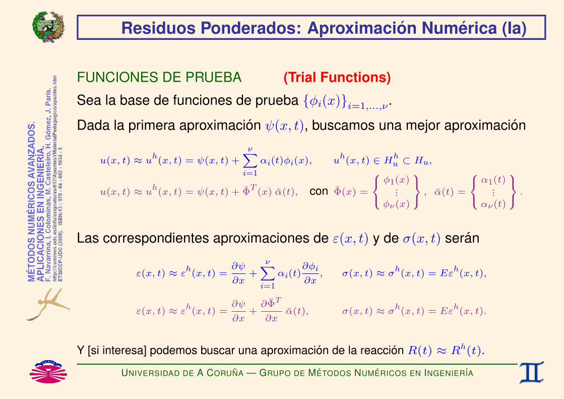
Residuos Ponderados: Aproximacion Numerica (Ia)
FUNCIONES DE PRUEBA (Trial Functions)
Sea la base de funciones de prueba φi(x)i=1,...,ν.
Dada la primera aproximacion ψ(x, t), buscamos una mejor aproximacion
u(x, t) ≈ uh(x, t) = ψ(x, t) +
νXi=1
αi(t)φi(x), uh(x, t) ∈ Hh
u ⊂ Hu,
u(x, t) ≈ uh(x, t) = ψ(x, t) + Φ
T(x) α(t), con Φ(x) =
8<:φ1(x)
...φν(x)
9=; , α(t) =
8<:α1(t)
...αν(t)
9=; .
Las correspondientes aproximaciones de ε(x, t) y de σ(x, t) seran
ε(x, t) ≈ εh(x, t) =
∂ψ
∂x+
νXi=1
αi(t)∂φi
∂x, σ(x, t) ≈ σ
h(x, t) = Eε
h(x, t),
ε(x, t) ≈ εh(x, t) =
∂ψ
∂x+∂ΦT
∂xα(t), σ(x, t) ≈ σ
h(x, t) = Eε
h(x, t).
Y [si interesa] podemos buscar una aproximacion de la reaccion R(t) ≈ Rh(t).
UNIVERSIDAD DE A CORUNA — GRUPO DE METODOS NUMERICOS EN INGENIERIA

Residuos Ponderados: Aproximacion Numerica (Ib)
En general no sera posible que uh(x, t) = u(x, t) ∀x ∈ [0, L] (*), por lo que
uh(x, t) 6= u(x, t)
m
no es posible que
∫ L
0
∂ω
∂xAσh dx =
∫ L
0
ωA
b+ ρcE∂uh
∂t
dx
+ ω(L)F (t) + ω(0)Rh(t) ∀ω(x) ∈ Hω.
(*) Salvo que u(x, t)− ψ(x, t) este contenido en el subespacio generado por las funciones de prueba.
UNIVERSIDAD DE A CORUNA — GRUPO DE METODOS NUMERICOS EN INGENIERIA

Residuos Ponderados: Aproximacion Numerica (IIa)
FUNCIONES DE TEST (Test Functions)
Sea la base de funciones de test ωj(x)j=1,...,ν.
Seaωh(x) =
νXj=1
βjωj(x), ωh(x) ∈ Hh
ω ⊂ Hω,
ωh(x) = Ω
T(x) β = β
TΩ(x), con Ω(x) =
8<:ω1(x)
...ων(x)
9=; , β =
8<:β1...βν
9=; .
Nos proponemos obtener la aproximacion uh(x, t) ∈ Hhu
∣∣∣ uh(0, t) = u0(t)
[y la aproximacion Rh] que verifique
Z L
0
∂ωh
∂xAσ
hdx =
Z L
0ωhA
0B@b+ ρcE∂uh
∂t
1CA dx
+ ωh(L)F (t) + ω
h(0)R
h(t) ∀ω(x) ∈ Hω,
uh(x, 0) = uI(x).
UNIVERSIDAD DE A CORUNA — GRUPO DE METODOS NUMERICOS EN INGENIERIA

Residuos Ponderados: Aproximacion Numerica (IIb)
PeroZ L
0
∂ωh
∂xAσ
hdx−
Z L
0ωhA
0B@b+ ρcE∂uh
∂t
1CA dx− ωh(L)F − ω
h(0)R
h= 0 ∀ωh(x) ∈ Hh
ω
m
νXj=1
βj
0B@Z L
0
∂ωj
∂xAσ
hdx−
Z L
0ωjA
0B@b+ ρcE∂uh
∂t
1CA dx− ωj(L)F − ωj(0)Rh
1CA = 0 ∀˘βj¯
βT
0B@Z L
0
∂Ω
∂xAσ
hdx−
Z L
0ΩA
0B@b+ ρcE∂uh
∂t
1CA dx− Ω(L)F − Ω(0)Rh
1CA = 0 ∀β
m
Z L
0
∂ωj
∂xAσ
hdx =
Z L
0ωjA
0B@b+ ρcE∂uh
∂t
1CA dx+ ωj(L)F + ωj(0)Rh, j=1,...,ν
Z L
0
∂Ω
∂xAσ
hdx =
Z L
0ΩA
0B@b+ ρcE∂uh
∂t
1CA dx+ Ω(L)F + Ω(0)Rh.
UNIVERSIDAD DE A CORUNA — GRUPO DE METODOS NUMERICOS EN INGENIERIA

Residuos Ponderados: Aproximacion Numerica (IIIa1)
Por tanto,
Z L
0
∂ωj
∂xAE
∂ψ
∂x+
νXi=1
αi∂φi
∂x
!dx =
Z L
0ωjA
0BB@b+ ρcE
∂ψ
∂t+
νXi=1
∂αi
∂tφi
! 1CCA dx+ ωj(L)F
+ ωj(0)Rh, j=1,...,ν
Z L
0
∂Ω
∂xAE
∂ψ
∂x+∂ΦT
∂xα
!dx =
Z L
0ΩA
0@b+ ρcE
„∂ψ
∂t+ Φ
T ∂α
∂t
« 1A dx+ Ω(L)F
+ Ω(0)Rh
UNIVERSIDAD DE A CORUNA — GRUPO DE METODOS NUMERICOS EN INGENIERIA

Residuos Ponderados: Aproximacion Numerica (IIIa2). . . luego,
−νXi=1
cjiz | Z L
0ωjAρcEφi dx
!∂αi
∂t+
νXi=1
kjiz | Z L
0
∂ωj
∂xAE
∂φi
∂xdx
!αi =
−Z L
0
∂ωj
∂xAE
∂ψ
∂xdx+
Z L
0ωjAb dx+
Z L
0ωjAρcE
∂ψ
∂tdx + ωj(L)F
| z fj(t)
+ ωj(0)Rh(t), j=1,...,ν
−
Cez | Z L
0ΩAρcEΦ
Tdx
!∂α
∂t+
Kez | Z L
0
∂Ω
∂xAE
∂ΦT
∂xdx
!α =
−Z L
0
∂Ω
∂xAE
∂ψ
∂xdx+
Z L
0ΩAb dx+
Z L
0ΩAρcE
∂ψ
∂tdx + Ω(L)F
| z f(t)
+ Ω(0)Rh(t)
UNIVERSIDAD DE A CORUNA — GRUPO DE METODOS NUMERICOS EN INGENIERIA

Residuos Ponderados: Aproximacion Numerica (IIIa3)
. . . y finalmente,
−ν∑i=1
cji∂αi(t)∂t
+ν∑i=1
kji αi(t) = fj(t) + ωj(0)Rh(t), j=1,...,ν
m
−C˜ ∂α(t)∂t
+K˜ α(t) = f(t) + Ω(0)Rh(t).
UNIVERSIDAD DE A CORUNA — GRUPO DE METODOS NUMERICOS EN INGENIERIA

Residuos Ponderados: Aproximacion Numerica (IIIb)
Luego el problema de equilibrio original ha sido sustituido por el sistema(de orden ν, con la incognita adicional Rh)
−C˜ ˙α(t) +K˜ α(t) = f(t) + Ω(0)Rh(t),
con la condicion de contorno esencial uh(0, t) = u0(t), esto es
ΦT (0) α(t) = u0(t)− ψ(0, t),
y con la condicion inicial uh(x, 0) = uI(x), esto es
ΦT (x) α(0) = uI(x)− ψ(x, 0).
UNIVERSIDAD DE A CORUNA — GRUPO DE METODOS NUMERICOS EN INGENIERIA

Residuos Ponderados: Aproximacion Numerica (IVa)
Si
• elegimos la primera aproximacion ψ(x, t) de forma que satisfaga la condicion decontorno esencial y las condiciones iniciales,
• elegimos las funciones de prueba φi(x) de forma que se anulen en los puntoscorrespondientes a las condiciones de contorno esenciales, y
• adoptamos como valores iniciales α(0) = 0,entonces la aproximacion uh(x, t) verificara automaticamente la condicion de contornoesencial y las condiciones iniciales, es decir
ψ(0, t) = u0(t)
Φ(0) = 0
9=; =⇒uh(0, t) = u0(t),
ψ(x, 0) = uI(x)
α(0) = 0
9=; =⇒uh(x, 0) = uI(x).
Si ademas elegimos las funciones de test ωj(x) de forma que se anulen en los puntoscorrespondientes a las condiciones de contorno esenciales, entonces la reaccion Rh(t) nointerviene en la formulacion.
UNIVERSIDAD DE A CORUNA — GRUPO DE METODOS NUMERICOS EN INGENIERIA

Residuos Ponderados: Aproximacion Numerica (IVb)
Por tanto, el sistema se reduce a
C˜ ˙α(t) −K˜ α(t) + f(t) = 0,
α(0) = 0 ,
que es un PROBLEMA DE VALOR INICIAL (PVI). (*)
(*) En este caso es sistema de ecuaciones diferenciales ordinarias (EDOs) de primer orden.
UNIVERSIDAD DE A CORUNA — GRUPO DE METODOS NUMERICOS EN INGENIERIA

Residuos Ponderados: Aproximacion Numerica (V)
Una vez resuelto el problema anterior obtendremos la aproximacion a lasolucion
uh(x, t) = ψ(x, t) +ν∑i=0
αi(t)φi(x) ⇐⇒ uh(x, t) = ψ(x, t) + ΦT (x) α(t).
εh(x, t) =∂ψ
∂x+
ν∑i=1
αi(t)∂φi∂x
⇐⇒ εh(x, t) =∂ψ
∂x+∂ΦT
∂xα(t)
σh(x, t) = Eεh(x, t) ⇐⇒ σh(x, t) = Eεh(x, t).
UNIVERSIDAD DE A CORUNA — GRUPO DE METODOS NUMERICOS EN INGENIERIA

Metodo de Bubnov-Galerkin (Ia)
PONDERACION DE BUBNOV–GALERKIN
Si se eligen como funciones de test las funciones de prueba, esto es
Hhω = Hh
u
mωj(x) = φj(x), j=0,...,ν ⇐⇒ Ω(x) = Φ(x),
C˜ ˙α(t) −K˜ α(t) + f(t) = 0,
α(0) = 0 ,
con . . .
UNIVERSIDAD DE A CORUNA — GRUPO DE METODOS NUMERICOS EN INGENIERIA

Metodo de Bubnov-Galerkin (Ib)
. . .
Ke =ˆkji˜i=1,...,νj=1,...,ν
, kji =
Z L
0
∂φj∂x AE
∂φi∂x dx
Ke =
Z L
0
∂Φ∂xAE
∂ΦT
∂x dx
Ce =ˆcji˜i=1,...,νj=1,...,ν
, cji =
Z L
0φjAρcEφi dx
Ce =
Z L
0ΦAρcEΦ
Tdx
f =˘fj¯j=1,...,ν
, fj = −Z L
0
∂φj∂x AE
∂ψ∂x dx+
Z L
0φjAb dx+
Z L
0φjAρcE
∂ψ
∂tdx + φj(L)F
f = −Z L
0
∂Φ∂xAE
∂ψ∂x dx+
Z L
0ΦAb dx+
Z L
0ΦAρcE
∂ψ
∂tdx + Φ(L)F.
UNIVERSIDAD DE A CORUNA — GRUPO DE METODOS NUMERICOS EN INGENIERIA

Metodo de Bubnov-Galerkin (Ic)
Esto es
Ke =
26666666664
Z L
0
∂φ1
∂xAE
∂φ1
∂xdx
Z L
0
∂φ1
∂xAE
∂φ2
∂xdx . . .
Z L
0
∂φ1
∂xAE
∂φν
∂xdxZ L
0
∂φ2
∂xAE
∂φ1
∂xdx
Z L
0
∂φ2
∂xAE
∂φ2
∂xdx . . .
Z L
0
∂φ2
∂xAE
∂φν
∂xdx
... ... ...Z L
0
∂φν
∂xAE
∂φ1
∂xdx
Z L
0
∂φν
∂xAE
∂φ2
∂xdx . . .
Z L
0
∂φν
∂xAE
∂φν
∂xdx
37777777775
Ce =
26666666664
Z L
0φ1AρcEφ1 dx
Z L
0φ1AρcEφ2 dx . . .
Z L
0φ1AρcEφν dxZ L
0φ2AρcEφ1 dx
Z L
0φ2AρcEφ2 dx . . .
Z L
0φ2AρcEφν dx
... ... ...Z L
0φνAρcEφ1 dx
Z L
0φνAρcEφ2 dx . . .
Z L
0φνAρcEφν dx
37777777775
UNIVERSIDAD DE A CORUNA — GRUPO DE METODOS NUMERICOS EN INGENIERIA

Metodo de Bubnov-Galerkin (Id)
f =
8>>>>>>>>>>>>>>>><>>>>>>>>>>>>>>>>:
−Z L
0
∂φ1
∂xAE
∂ψ
∂xdx+
Z L
0φ1Ab dx+
Z L
0φ1AρcE
∂ψ
∂tdx + φ1(L)F
−Z L
0
∂φ2
∂xAE
∂ψ
∂xdx+
Z L
0φ2Ab dx+
Z L
0φ2AρcE
∂ψ
∂tdx + φ2(L)F
...
−Z L
0
∂φν
∂xAE
∂ψ
∂xdx+
Z L
0φνAb dx+
Z L
0φνAρcE
∂ψ
∂tdx + φν(L)F
9>>>>>>>>>>>>>>>>=>>>>>>>>>>>>>>>>;
.
UNIVERSIDAD DE A CORUNA — GRUPO DE METODOS NUMERICOS EN INGENIERIA

Metodo de Bubnov-Galerkin (IIa)
La matriz (−K˜ ) del metodo de Galerkin es. . . (*)
♥ SIMETRICA(−K˜ ) = (−K˜ )T
♥ SEMIDEFINIDA POSITIVA
wT (−K˜ ) w ≥ 0 ∀w 6= 0
♥ DEFINIDA POSITIVA
wT (−K˜ ) w > 0 ∀w 6= 0 (**)
(*) En este caso se trabaja con −Ke porque E = −γ.
(**) Si la base de funciones de prueba ha sido correctamente elegida.
UNIVERSIDAD DE A CORUNA — GRUPO DE METODOS NUMERICOS EN INGENIERIA

Metodo de Bubnov-Galerkin (IIb)
(-K˜ ) es SIMETRICA, ya que
(−kji) =
Z L
0
∂φj
∂xAγ
∂φi
∂xdx =
Z L
0
∂φi
∂xAγ
∂φj
∂xdx = (−kij)
m
(−Ke ) =
Z L
0
∂Φ
∂xAγ
∂ΦT
∂xdx =
Z L
0
∂Φ
∂xAγ
∂ΦT
∂x
!T
dx =
Z L
0
∂Φ
∂xAγ
∂ΦT
∂xdx
!T
= (−Ke )T.
UNIVERSIDAD DE A CORUNA — GRUPO DE METODOS NUMERICOS EN INGENIERIA

Metodo de Bubnov-Galerkin (IIc)
(-K˜ ) es SEMIDEFINIDA POSITIVA, ya que
νXj=1
νXi=1
wj(−kji)wi =νXj=1
νXi=1
wj
Z L
0
∂φj
∂xAγ
∂φi
∂xdx
!wi =
Z L
0
0@ νXj=1
wj∂φj
∂x
1A| z
g(x)
Aγ
νXi=1
wi∂φi
∂x
!| z
g(x)
dx
=
Z L
0
νXi=1
wi∂φi
∂x
!2
Aγ dx ≥ 0 ∀w = wii=1,...,ν 6= 0.
m
wT(−Ke )w = w
T
Z L
0
∂Φ
∂xAγ
∂ΦT
∂xdx
!w =
Z L
0
∂ΦT
∂xw
!| z
g(x)
Aγ
∂ΦT
∂xw
!| z
g(x)
dx
=
Z L
0
∂ΦT
∂xw
!2
Aγ dx ≥ 0 ∀w 6= 0.
UNIVERSIDAD DE A CORUNA — GRUPO DE METODOS NUMERICOS EN INGENIERIA

Metodo de Bubnov-Galerkin (IId)
(-K˜ ) es DEFINIDA POSITIVA, ya que (vease el punto anterior)
νXj=1
νXi=1
wj(−kji)wi = 0 =⇒νXi=1
wi∂φi
∂x= 0 ∀x ∈ [0, L] =⇒ wi = 0, i = 1, . . . , ν
m
wT(−Ke )w = 0 =⇒
∂ΦT
∂xw = 0 ∀x ∈ [0, L] =⇒ w = 0.
si la base de funciones de prueba ha sido correctamente elegida (de formaque sus derivadas sean linealmente independientes).
UNIVERSIDAD DE A CORUNA — GRUPO DE METODOS NUMERICOS EN INGENIERIA
Metodo de Bubnov-Galerkin (IIIa)
La matriz C˜ del metodo de Galerkin tiene la misma forma que la matriz(−K˜ ) (con identicos anchos de banda y perfiles de filas y columnas) ytambien es. . .
♥ SIMETRICAC˜ = C˜T
♥ SEMIDEFINIDA POSITIVA
wTC˜ w ≥ 0 ∀w 6= 0
♥ DEFINIDA POSITIVA
wTC˜ w > 0 ∀w 6= 0 (*)
(*) Si la base de funciones de prueba ha sido correctamente elegida.
UNIVERSIDAD DE A CORUNA — GRUPO DE METODOS NUMERICOS EN INGENIERIA

Metodo de Bubnov-Galerkin (IIIb)
C˜ es SIMETRICA, ya que
cji =
Z L
0
φjAρcEφi dx =
Z L
0
φiAρcEφj dx = cij
m
Ce =
Z L
0
ΦAρcEΦTdx =
Z L
0
“ΦAρcEΦ
T”T
dx =
Z L
0
ΦAρcEΦTdx
!T
= CeT .
UNIVERSIDAD DE A CORUNA — GRUPO DE METODOS NUMERICOS EN INGENIERIA

Metodo de Bubnov-Galerkin (IIIc)
C˜ es SEMIDEFINIDA POSITIVA, ya que
νXj=1
νXi=1
wjcjiwi =νXj=1
νXi=1
wj
Z L
0φjAρcEφi dx
!wi =
Z L
0
0@ νXj=1
wjφj
1A| z
g(x)
AρcE
νXi=1
wiφi
!| z
g(x)
dx
=
Z L
0
νXi=1
wiφi
!2
AρcE dx ≥ 0 ∀w = wii=1,...,ν 6= 0.
m
wTCew = w
T
Z L
0ΦAρcEΦ
Tdx
!w =
Z L
0
“ΦTw”
| z g(x)
AρcE
“ΦTw”
| z g(x)
dx
=
Z L
0
“ΦTw”2AρcE dx ≥ 0 ∀w 6= 0.
UNIVERSIDAD DE A CORUNA — GRUPO DE METODOS NUMERICOS EN INGENIERIA

Metodo de Bubnov-Galerkin (IIId)
C˜ es DEFINIDA POSITIVA, ya que (vease el punto anterior)
νXj=1
νXi=1
wjcjiwi = 0 =⇒νXi=1
wiφi = 0 ∀x ∈ [0, L] =⇒ wi = 0, i = 1, . . . , ν
m
wTKe w = 0 =⇒ Φ
Tw = 0 ∀x ∈ [0, L] =⇒ w = 0.
si la base de funciones de prueba ha sido correctamente elegida (de formaque sean linealmente independientes).
UNIVERSIDAD DE A CORUNA — GRUPO DE METODOS NUMERICOS EN INGENIERIA


METODO DE RESIDUOS PONDERADOS:PROBLEMAS NO ESTACIONARIOS 1D
DE TIPO HIPERBOLICOF. Navarrina, I. Colominas, M. Casteleiro, H. Gomez, J. Parıs
GMNI — GRUPO DE METODOS NUMERICOS EN INGENIERIA
Departamento de Metodos Matematicos y de RepresentacionEscuela Tecnica Superior de Ingenieros de Caminos, Canales y Puertos
Universidad de A Coruna, Espana
e-mail: [email protected] web: http://caminos.udc.es/gmni
UNIVERSIDAD DE A CORUNA — GRUPO DE METODOS NUMERICOS EN INGENIERIA

INDICE
I Problema Conceptual
I Residuos Ponderados: Forma Debil
I Residuos Ponderados: Aproximacion Numerica
I Metodo de Bubnov-Galerkin
UNIVERSIDAD DE A CORUNA — GRUPO DE METODOS NUMERICOS EN INGENIERIA

Problema Conceptual (I)
Sea el problema de equilibrio 1D:
UNIVERSIDAD DE A CORUNA — GRUPO DE METODOS NUMERICOS EN INGENIERIA
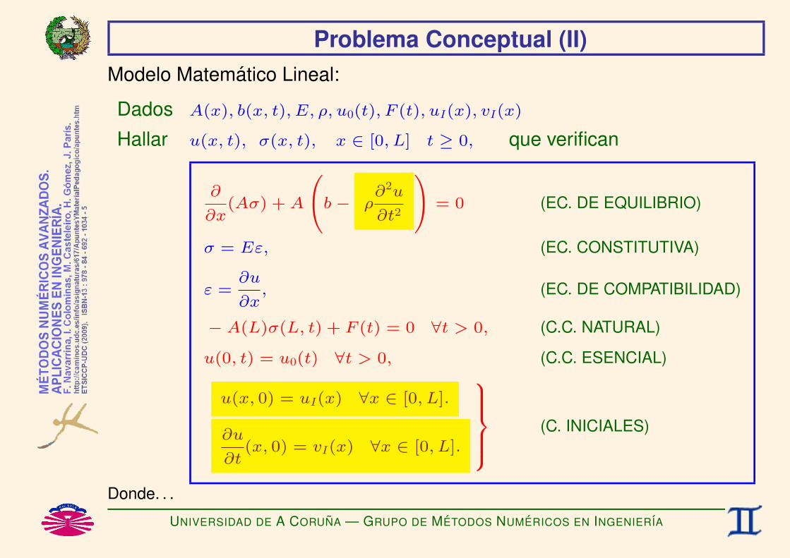
Problema Conceptual (II)Modelo Matematico Lineal:
Dados A(x), b(x, t), E, ρ, u0(t), F (t), uI(x), vI(x)
Hallar u(x, t), σ(x, t), x ∈ [0, L] t ≥ 0, que verifican
∂
∂x(Aσ) + A
0@b− ρ∂2u
∂t2
1A = 0 (EC. DE EQUILIBRIO)
σ = Eε, (EC. CONSTITUTIVA)
ε =∂u
∂x, (EC. DE COMPATIBILIDAD)
− A(L)σ(L, t) + F (t) = 0 ∀t > 0, (C.C. NATURAL)
u(0, t) = u0(t) ∀t > 0, (C.C. ESENCIAL)
u(x, 0) = uI(x) ∀x ∈ [0, L].
∂u
∂t(x, 0) = vI(x) ∀x ∈ [0, L].
9>>>=>>>; (C. INICIALES)
Donde. . .
UNIVERSIDAD DE A CORUNA — GRUPO DE METODOS NUMERICOS EN INGENIERIA

Problema Conceptual (III)
Barra elastica a traccion–compresion[0, L] = barra de longitud L.x ∈ [0, L] = coordenada material de un punto.t > 0 = tiempo.A(x) = seccion transversal.u(x, t) = DESPLAZAMIENTO.ε(x, t) = DEFORMACION.σ(x, t) = TENSION.b(x, t) = FUERZA EXTERIOR POR UNIDAD DE VOLUMEN.u0(t) = DESPLAZAMIENTO PREFIJADO EN x = 0.R(t) = −A(0)σ(0, t) (REACCION EN x = 0.)F (t) = A(L)σ(L, t) (FUERZA PUNTUAL EXTERIOR EN x = L.)uI(x) = DESPLAZAMIENTO INICIAL DE CADA PUNTO.vI(x) = VELOCIDAD INICIAL DE CADA PUNTO.E = MODULO DE ELASTICIDAD.ρ = DENSIDAD.
En este caso, la ecuacion constitutiva se denomina LEY DE HOOKE.
UNIVERSIDAD DE A CORUNA — GRUPO DE METODOS NUMERICOS EN INGENIERIA
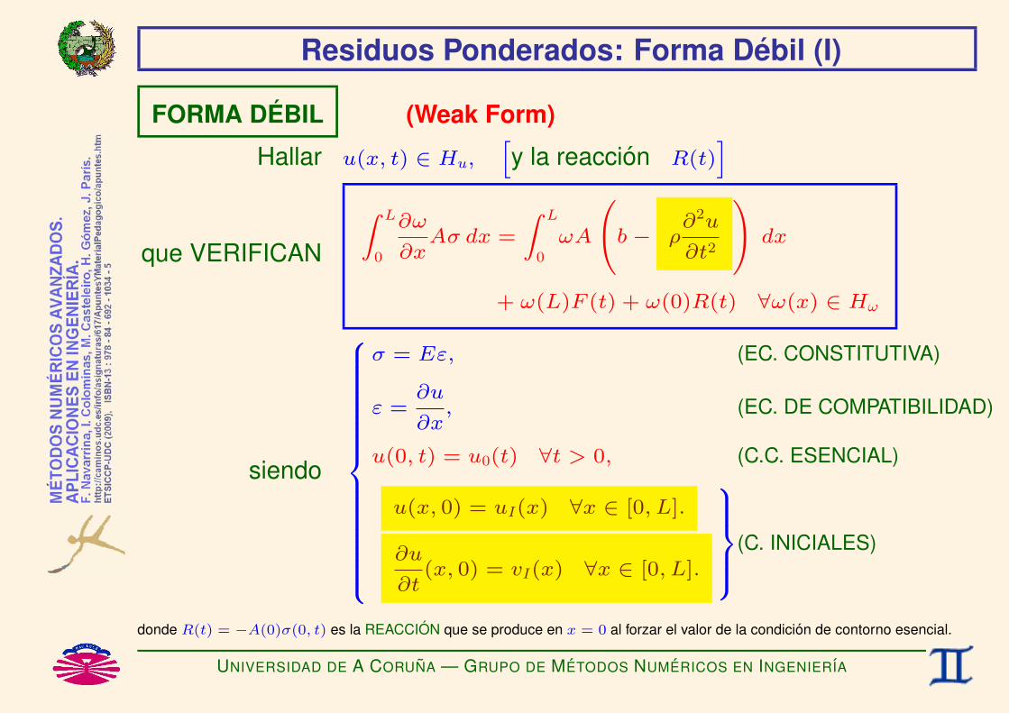
Residuos Ponderados: Forma Debil (I)
FORMA DEBIL (Weak Form)
Hallar u(x, t) ∈ Hu,hy la reaccion R(t)
i
que VERIFICAN
Z L
0
∂ω
∂xAσ dx =
Z L
0
ωA
0@b− ρ∂2u
∂t2
1A dx
+ ω(L)F (t) + ω(0)R(t) ∀ω(x) ∈ Hω
siendo
8>>>>>>>>>>>>>>><>>>>>>>>>>>>>>>:
σ = Eε, (EC. CONSTITUTIVA)
ε =∂u
∂x, (EC. DE COMPATIBILIDAD)
u(0, t) = u0(t) ∀t > 0, (C.C. ESENCIAL)
u(x, 0) = uI(x) ∀x ∈ [0, L].
∂u
∂t(x, 0) = vI(x) ∀x ∈ [0, L].
9>>>=>>>;(C. INICIALES)
donde R(t) = −A(0)σ(0, t) es la REACCION que se produce en x = 0 al forzar el valor de la condicion de contorno esencial.
UNIVERSIDAD DE A CORUNA — GRUPO DE METODOS NUMERICOS EN INGENIERIA

Residuos Ponderados: Aproximacion Numerica (Ia)
FUNCIONES DE PRUEBA (Trial Functions)
Sea la base de funciones de prueba φi(x)i=1,...,ν.
Dada la primera aproximacion ψ(x, t), buscamos una mejor aproximacion
u(x, t) ≈ uh(x, t) = ψ(x, t) +
νXi=1
αi(t)φi(x), uh(x, t) ∈ Hh
u ⊂ Hu,
u(x, t) ≈ uh(x, t) = ψ(x, t) + Φ
T(x) α(t), con Φ(x) =
8<:φ1(x)
...φν(x)
9=; , α(t) =
8<:α1(t)
...αν(t)
9=; .
Las correspondientes aproximaciones de ε(x, t) y de σ(x, t) seran
ε(x, t) ≈ εh(x, t) =
∂ψ
∂x+
νXi=1
αi(t)∂φi
∂x, σ(x, t) ≈ σ
h(x, t) = Eε
h(x, t),
ε(x, t) ≈ εh(x, t) =
∂ψ
∂x+∂ΦT
∂xα(t), σ(x, t) ≈ σ
h(x, t) = Eε
h(x, t).
Y [si interesa] podemos buscar una aproximacion de la reaccion R(t) ≈ Rh(t).
UNIVERSIDAD DE A CORUNA — GRUPO DE METODOS NUMERICOS EN INGENIERIA

Residuos Ponderados: Aproximacion Numerica (Ib)
En general no sera posible que uh(x, t) = u(x, t) ∀x ∈ [0, L] (*), por lo que
uh(x, t) 6= u(x, t)
m
no es posible que
∫ L
0
∂ω
∂xAσh dx =
∫ L
0
ωA
b− ρ∂2uh
∂t2
dx
+ ω(L)F (t) + ω(0)Rh(t) ∀ω(x) ∈ Hω.
(*) Salvo que u(x, t)− ψ(x, t) este contenido en el subespacio generado por las funciones de prueba.
UNIVERSIDAD DE A CORUNA — GRUPO DE METODOS NUMERICOS EN INGENIERIA

Residuos Ponderados: Aproximacion Numerica (IIa)
FUNCIONES DE TEST (Test Functions)
Sea la base de funciones de test ωj(x)j=1,...,ν.
Seaωh(x) =
νXj=1
βjωj(x), ωh(x) ∈ Hh
ω ⊂ Hω,
ωh(x) = Ω
T(x) β = β
TΩ(x), con Ω(x) =
8<:ω1(x)
...ων(x)
9=; , β =
8<:β1...βν
9=; .
Nos proponemos obtener la aproximacion uh(x, t) ∈ Hhu
∣∣∣ uh(0, t) = u0(t)
[y la aproximacion Rh] que verifique
Z L
0
∂ωh
∂xAσ
hdx =
Z L
0ωhA
0B@b− ρ∂2uh
∂t2
1CA dx
+ ωh(L)F (t) + ω
h(0)R
h(t) ∀ω(x) ∈ Hω,
uh(x, 0) = uI(x),
∂uh
∂t(x, 0) = vI(x),
UNIVERSIDAD DE A CORUNA — GRUPO DE METODOS NUMERICOS EN INGENIERIA

Residuos Ponderados: Aproximacion Numerica (IIb)
PeroZ L
0
∂ωh
∂xAσ
hdx−
Z L
0ωhA
0B@b− ρ∂2uh
∂t2
1CA dx− ωh(L)F − ω
h(0)R
h= 0 ∀ωh(x) ∈ Hh
ω
m
νXj=1
βj
0B@Z L
0
∂ωj
∂xAσ
hdx−
Z L
0ωjA
0B@b− ρ∂2uh
∂t2
1CA dx− ωj(L)F − ωj(0)Rh
1CA = 0 ∀˘βj¯
βT
0B@Z L
0
∂Ω
∂xAσ
hdx−
Z L
0ΩA
0B@b− ρ∂2uh
∂t2
1CA dx− Ω(L)F − Ω(0)Rh
1CA = 0 ∀β
m
Z L
0
∂ωj
∂xAσ
hdx =
Z L
0ωjA
0B@b− ρ∂2uh
∂t2
1CA dx+ ωj(L)F + ωj(0)Rh, j=1,...,ν
Z L
0
∂Ω
∂xAσ
hdx =
Z L
0ΩA
0B@b− ρ∂2uh
∂t2
1CA dx+ Ω(L)F + Ω(0)Rh.
UNIVERSIDAD DE A CORUNA — GRUPO DE METODOS NUMERICOS EN INGENIERIA

Residuos Ponderados: Aproximacion Numerica (IIIa1)
Por tanto,
Z L
0
∂ωj
∂xAE
∂ψ
∂x+
νXi=1
αi∂φi
∂x
!dx =
Z L
0ωjA
0BB@b− ρ
∂2ψ
∂t2+
νXi=1
∂2αi
∂t2φi
! 1CCA dx+ ωj(L)F
+ ωj(0)Rh, j=1,...,ν
Z L
0
∂Ω
∂xAE
∂ψ
∂x+∂ΦT
∂xα
!dx =
Z L
0ΩA
0B@b− ρ
∂2ψ
∂t2+ Φ
T ∂2α
∂t2
! 1CA dx+ Ω(L)F
+ Ω(0)Rh
UNIVERSIDAD DE A CORUNA — GRUPO DE METODOS NUMERICOS EN INGENIERIA

Residuos Ponderados: Aproximacion Numerica (IIIa2). . . luego,
νXi=1
mjiz | Z L
0ωjAρφi dx
!∂2αi
∂t2+
νXi=1
kjiz | Z L
0
∂ωj
∂xAE
∂φi
∂xdx
!αi =
−Z L
0
∂ωj
∂xAE
∂ψ
∂xdx+
Z L
0ωjAb dx−
Z L
0ωjAρ
∂2ψ
∂t2dx + ωj(L)F
| z fj(t)
+ ωj(0)Rh(t), j=1,...,ν
Mez | Z L
0ΩAρΦ
Tdx
!∂2α
∂t2+
Kez | Z L
0
∂Ω
∂xAE
∂ΦT
∂xdx
!α =
−Z L
0
∂Ω
∂xAE
∂ψ
∂xdx+
Z L
0ΩAb dx−
Z L
0ΩAρ
∂2ψ
∂t2dx + Ω(L)F
| z f(t)
+ Ω(0)Rh(t)
UNIVERSIDAD DE A CORUNA — GRUPO DE METODOS NUMERICOS EN INGENIERIA

Residuos Ponderados: Aproximacion Numerica (IIIa3)
. . . y finalmente,
ν∑i=1
mji∂2αi(t)∂t2
+ν∑i=1
kji αi(t) = fj(t) + ωj(0)Rh(t), j=1,...,ν
m
M˜ ∂2α(t)∂t2
+K˜ α(t) = f(t) + Ω(0)Rh(t).
UNIVERSIDAD DE A CORUNA — GRUPO DE METODOS NUMERICOS EN INGENIERIA
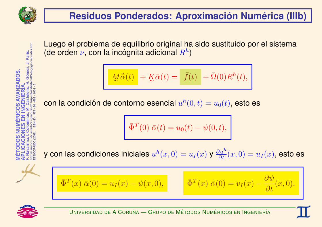
Residuos Ponderados: Aproximacion Numerica (IIIb)
Luego el problema de equilibrio original ha sido sustituido por el sistema(de orden ν, con la incognita adicional Rh)
M˜ ¨α(t) +K˜ α(t) = f(t) + Ω(0)Rh(t),
con la condicion de contorno esencial uh(0, t) = u0(t), esto es
ΦT (0) α(t) = u0(t)− ψ(0, t),
y con las condiciones iniciales uh(x, 0) = uI(x) y ∂uh
∂t (x, 0) = uI(x), esto es
ΦT (x) α(0) = uI(x)− ψ(x, 0), ΦT (x) ˙α(0) = vI(x)−∂ψ
∂t(x, 0).
UNIVERSIDAD DE A CORUNA — GRUPO DE METODOS NUMERICOS EN INGENIERIA

Residuos Ponderados: Aproximacion Numerica (IVa)
Si
• elegimos la primera aproximacion ψ(x, t) de forma que satisfaga la condicion decontorno esencial y las condiciones iniciales,
• elegimos las funciones de prueba φi(x) de forma que se anulen en los puntoscorrespondientes a las condiciones de contorno esenciales, y
• adoptamos como valores iniciales α(0) = 0 y ˙α(0) = 0
entonces la aproximacion uh(x, t) verificara automaticamente la condicion de contornoesencial y las condiciones iniciales, es decir
ψ(0, t) = u0(t)
Φ(0) = 0
)=⇒uh(0, t) = u0(t),
ψ(x, 0) = uI(x),∂ψ
∂t(x, 0) = vI(x)
α(0) = 0, ˙α(0) = 0
)=⇒uh(x, 0) = uI(x),
∂uh
∂t(x, 0) = vI(x).
Si ademas elegimos las funciones de test ωj(x) de forma que se anulen en los puntoscorrespondientes a las condiciones de contorno esenciales, entonces la reaccion Rh(t) nointerviene en la formulacion.
UNIVERSIDAD DE A CORUNA — GRUPO DE METODOS NUMERICOS EN INGENIERIA

Residuos Ponderados: Aproximacion Numerica (IVb)
Por tanto, el sistema se reduce a
M˜ ¨α(t) +K˜ α(t)− f(t) = 0,
α(0) = 0 , ˙α(0) = 0 ,
que es un PROBLEMA DE VALOR INICIAL (PVI). (*)
(*) En este caso es sistema de ecuaciones diferenciales ordinarias (EDOs) de segundo orden.
UNIVERSIDAD DE A CORUNA — GRUPO DE METODOS NUMERICOS EN INGENIERIA
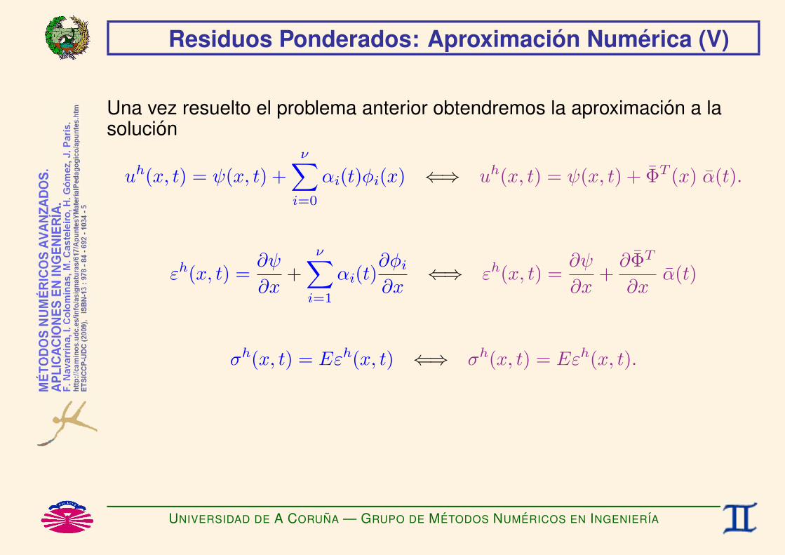
Residuos Ponderados: Aproximacion Numerica (V)
Una vez resuelto el problema anterior obtendremos la aproximacion a lasolucion
uh(x, t) = ψ(x, t) +ν∑i=0
αi(t)φi(x) ⇐⇒ uh(x, t) = ψ(x, t) + ΦT (x) α(t).
εh(x, t) =∂ψ
∂x+
ν∑i=1
αi(t)∂φi∂x
⇐⇒ εh(x, t) =∂ψ
∂x+∂ΦT
∂xα(t)
σh(x, t) = Eεh(x, t) ⇐⇒ σh(x, t) = Eεh(x, t).
UNIVERSIDAD DE A CORUNA — GRUPO DE METODOS NUMERICOS EN INGENIERIA

Residuos Ponderados: Aproximacion Numerica (VI)
ESTUDIO DE VIBRACIONES LIBRES
M˜ ¨α(t) +K˜ α(t) = 0.
Buscamos soluciones de la forma α(t) = aejωt, para las que(−ω2M˜ a+K˜ a
)ejωt = 0,
y se obtiene el problema generalizado de VALORES PROPIOS
K˜ a = λM˜ a, con λ = ω2.
UNIVERSIDAD DE A CORUNA — GRUPO DE METODOS NUMERICOS EN INGENIERIA

Metodo de Bubnov-Galerkin (Ia)
PONDERACION DE BUBNOV–GALERKIN
Si se eligen como funciones de test las funciones de prueba, esto es
Hhω = Hh
u
mωj(x) = φj(x), j=0,...,ν ⇐⇒ Ω(x) = Φ(x),
M˜ ¨α(t) +K˜ α(t)− f(t) = 0,
α(0) = 0, ˙α(0) = 0.
con . . .
UNIVERSIDAD DE A CORUNA — GRUPO DE METODOS NUMERICOS EN INGENIERIA

Metodo de Bubnov-Galerkin (Ib)
. . .
Ke =ˆkji˜i=1,...,νj=1,...,ν
, kji =
Z L
0
∂φj∂x AE
∂φi∂x dx
Ke =
Z L
0
∂Φ∂xAE
∂ΦT
∂x dx
Me =ˆmji
˜i=1,...,νj=1,...,ν
, mji =
Z L
0φjAρφi dx
Me =
Z L
0ΦAρΦ
Tdx
f =˘fj¯j=1,...,ν
, fj = −Z L
0
∂φj∂x AE
∂ψ∂x dx+
Z L
0φjAb dx−
Z L
0φjAρ
∂2ψ
∂t2dx + φj(L)F
f = −Z L
0
∂Φ∂xAE
∂ψ∂x dx+
Z L
0ΦAb dx−
Z L
0ΦAρ
∂2ψ
∂t2dx + Φ(L)F.
UNIVERSIDAD DE A CORUNA — GRUPO DE METODOS NUMERICOS EN INGENIERIA

Metodo de Bubnov-Galerkin (Ic)
Esto es
Ke =
26666666664
Z L
0
∂φ1
∂xAE
∂φ1
∂xdx
Z L
0
∂φ1
∂xAE
∂φ2
∂xdx . . .
Z L
0
∂φ1
∂xAE
∂φν
∂xdxZ L
0
∂φ2
∂xAE
∂φ1
∂xdx
Z L
0
∂φ2
∂xAE
∂φ2
∂xdx . . .
Z L
0
∂φ2
∂xAE
∂φν
∂xdx
... ... ...Z L
0
∂φν
∂xAE
∂φ1
∂xdx
Z L
0
∂φν
∂xAE
∂φ2
∂xdx . . .
Z L
0
∂φν
∂xAE
∂φν
∂xdx
37777777775
Me =
26666666664
Z L
0φ1Aρφ1 dx
Z L
0φ1Aρφ2 dx . . .
Z L
0φ1Aρφν dxZ L
0φ2Aρφ1 dx
Z L
0φ2Aρφ2 dx . . .
Z L
0φ2Aρφν dx
... ... ...Z L
0φνAρφ1 dx
Z L
0φνAρφ2 dx . . .
Z L
0φνAρφν dx
37777777775
UNIVERSIDAD DE A CORUNA — GRUPO DE METODOS NUMERICOS EN INGENIERIA

Metodo de Bubnov-Galerkin (Id)
f =
8>>>>>>>>>>>>>>>><>>>>>>>>>>>>>>>>:
−Z L
0
∂φ1
∂xAE
∂ψ
∂xdx+
Z L
0φ1Ab dx−
Z L
0φ1Aρ
∂2ψ
∂t2dx + φ1(L)F
−Z L
0
∂φ2
∂xAE
∂ψ
∂xdx+
Z L
0φ2Ab dx−
Z L
0φ2Aρ
∂2ψ
∂t2dx + φ2(L)F
...
−Z L
0
∂φν
∂xAE
∂ψ
∂xdx+
Z L
0φνAb dx−
Z L
0φνAρ
∂2ψ
∂t2dx + φν(L)F
9>>>>>>>>>>>>>>>>=>>>>>>>>>>>>>>>>;
.
UNIVERSIDAD DE A CORUNA — GRUPO DE METODOS NUMERICOS EN INGENIERIA

Metodo de Bubnov-Galerkin (IIa)
La matriz K˜ del metodo de Galerkin es. . . (*)
♥ SIMETRICAK˜ = K˜ T
♥ SEMIDEFINIDA POSITIVA
wTK˜ w ≥ 0 ∀w 6= 0
♥ DEFINIDA POSITIVA
wTK˜ w > 0 ∀w 6= 0 (*)
(*) Si la base de funciones de prueba ha sido correctamente elegida.
UNIVERSIDAD DE A CORUNA — GRUPO DE METODOS NUMERICOS EN INGENIERIA
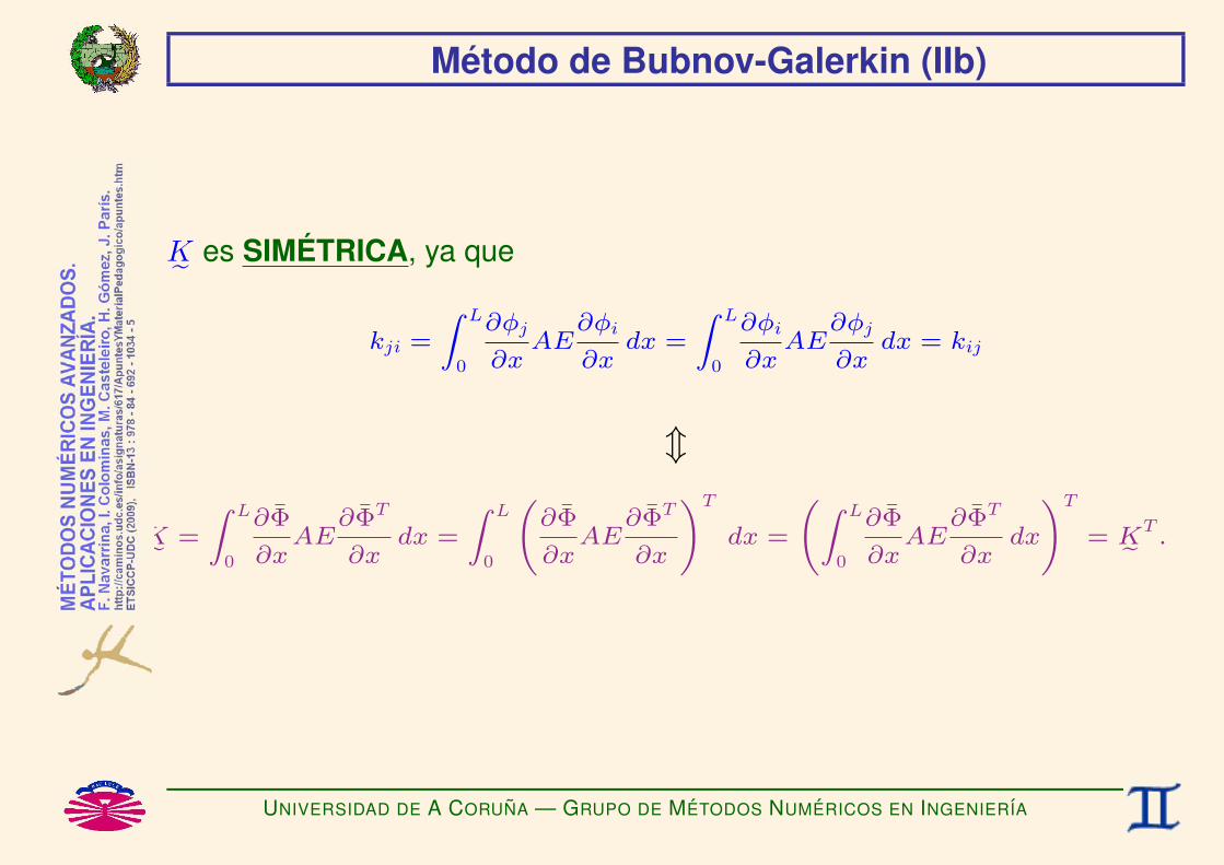
Metodo de Bubnov-Galerkin (IIb)
K˜ es SIMETRICA, ya que
kji =
Z L
0
∂φj
∂xAE
∂φi
∂xdx =
Z L
0
∂φi
∂xAE
∂φj
∂xdx = kij
m
Ke =
Z L
0
∂Φ
∂xAE
∂ΦT
∂xdx =
Z L
0
∂Φ
∂xAE
∂ΦT
∂x
!T
dx =
Z L
0
∂Φ
∂xAE
∂ΦT
∂xdx
!T
= Ke T .
UNIVERSIDAD DE A CORUNA — GRUPO DE METODOS NUMERICOS EN INGENIERIA

Metodo de Bubnov-Galerkin (IIc)
K˜ es SEMIDEFINIDA POSITIVA, ya que
νXj=1
νXi=1
wjkjiwi =νXj=1
νXi=1
wj
Z L
0
∂φj
∂xAE
∂φi
∂xdx
!wi =
Z L
0
0@ νXj=1
wj∂φj
∂x
1A| z
g(x)
AE
νXi=1
wi∂φi
∂x
!| z
g(x)
dx
=
Z L
0
νXi=1
wi∂φi
∂x
!2
AE dx ≥ 0 ∀w = wii=1,...,ν 6= 0.
m
wTKe w = w
T
Z L
0
∂Φ
∂xAE
∂ΦT
∂xdx
!w =
Z L
0
∂ΦT
∂xw
!| z
g(x)
AE
∂ΦT
∂xw
!| z
g(x)
dx
=
Z L
0
∂ΦT
∂xw
!2
AE dx ≥ 0 ∀w 6= 0.
UNIVERSIDAD DE A CORUNA — GRUPO DE METODOS NUMERICOS EN INGENIERIA

Metodo de Bubnov-Galerkin (IId)
K˜ es DEFINIDA POSITIVA, ya que (vease el punto anterior)
νXj=1
νXi=1
wjkjiwi = 0 =⇒νXi=1
wi∂φi
∂x= 0 ∀x ∈ [0, L] =⇒ wi = 0, i = 1, . . . , ν
m
wTKe w = 0 =⇒
∂ΦT
∂xw = 0 ∀x ∈ [0, L] =⇒ w = 0.
si la base de funciones de prueba ha sido correctamente elegida (de formaque sus derivadas sean linealmente independientes).
UNIVERSIDAD DE A CORUNA — GRUPO DE METODOS NUMERICOS EN INGENIERIA
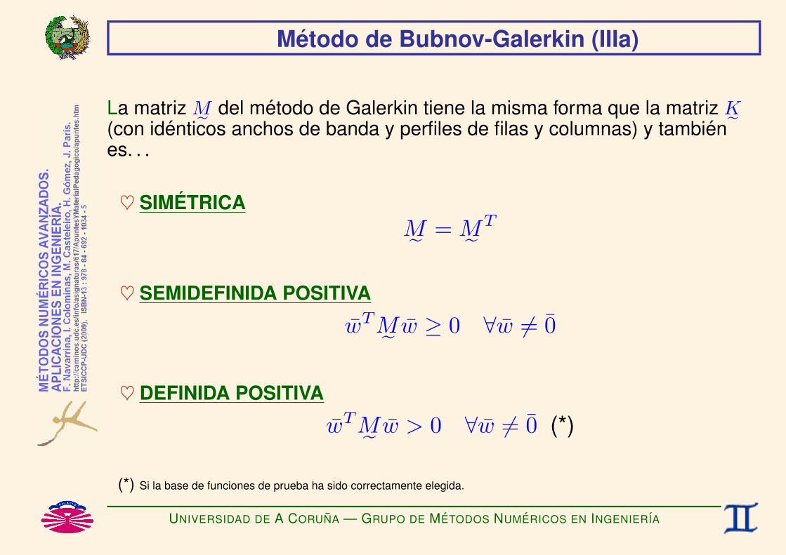
Metodo de Bubnov-Galerkin (IIIa)
La matriz M˜ del metodo de Galerkin tiene la misma forma que la matriz K˜(con identicos anchos de banda y perfiles de filas y columnas) y tambienes. . .
♥ SIMETRICAM˜ = M˜ T
♥ SEMIDEFINIDA POSITIVA
wTM˜ w ≥ 0 ∀w 6= 0
♥ DEFINIDA POSITIVA
wTM˜ w > 0 ∀w 6= 0 (*)
(*) Si la base de funciones de prueba ha sido correctamente elegida.
UNIVERSIDAD DE A CORUNA — GRUPO DE METODOS NUMERICOS EN INGENIERIA

Metodo de Bubnov-Galerkin (IIIb)
M˜ es SIMETRICA, ya que
mji =
Z L
0
φjAρφi dx =
Z L
0
φiAρφj dx = mij
m
Me =
Z L
0
ΦAρΦTdx =
Z L
0
“ΦAρΦ
T”T
dx =
Z L
0
ΦAρΦTdx
!T
= Me T.
UNIVERSIDAD DE A CORUNA — GRUPO DE METODOS NUMERICOS EN INGENIERIA
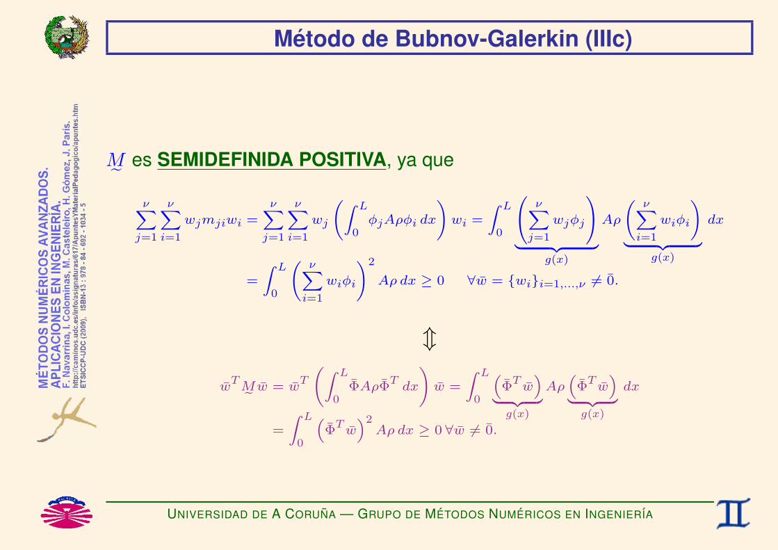
Metodo de Bubnov-Galerkin (IIIc)
M˜ es SEMIDEFINIDA POSITIVA, ya que
νXj=1
νXi=1
wjmjiwi =νXj=1
νXi=1
wj
Z L
0φjAρφi dx
!wi =
Z L
0
0@ νXj=1
wjφj
1A| z
g(x)
Aρ
νXi=1
wiφi
!| z
g(x)
dx
=
Z L
0
νXi=1
wiφi
!2
Aρdx ≥ 0 ∀w = wii=1,...,ν 6= 0.
m
wTMe w = w
T
Z L
0ΦAρΦ
Tdx
!w =
Z L
0
“ΦTw”
| z g(x)
Aρ“ΦTw”
| z g(x)
dx
=
Z L
0
“ΦTw”2Aρdx ≥ 0 ∀w 6= 0.
UNIVERSIDAD DE A CORUNA — GRUPO DE METODOS NUMERICOS EN INGENIERIA

Metodo de Bubnov-Galerkin (IIId)
M˜ es DEFINIDA POSITIVA, ya que (vease el punto anterior)
νXj=1
νXi=1
wjmjiwi = 0 =⇒νXi=1
wiφi = 0 ∀x ∈ [0, L] =⇒ wi = 0, i = 1, . . . , ν
m
wTMe w = 0 =⇒ Φ
Tw = 0 ∀x ∈ [0, L] =⇒ w = 0.
si la base de funciones de prueba ha sido correctamente elegida (de formaque sean linealmente independientes).
UNIVERSIDAD DE A CORUNA — GRUPO DE METODOS NUMERICOS EN INGENIERIA