Embed Size (px)
Citation preview

Escola Superior de Tecnologia de Tomar
Filipe Alexandre Guido Bandeiras
MICROGRID ARCHITECTURE EVALUATION FOR SMALL AND MEDIUM SIZE INDUSTRIES
Dissertação de Mestrado
Mestrado em Engenharia Eletrotécnica Especialização em Controlo e Eletrónica Industrial
Tomar/Novembro/2017


Escola Superior de Tecnologia de Tomar
Filipe Alexandre Guido Bandeiras
MICROGRID ARCHITECTURE EVALUATION FOR SMALL AND MEDIUM SIZE INDUSTRIES
Dissertação de Mestrado
Orientado por: Prof. Mário Gomes – IPT/ESTT Prof. Paulo Coelho – IPT/ESTT
Dissertação apresentada ao Instituto Politécnico de Tomar para o cumprimento dos requisitos necessários à obtenção do grau de Mestre em Engenharia Eletrotécnica –
Especialização em Controlo e Eletrónica Industrial


MICROGRID ARCHITECTURE EVALUATION FOR SMALL AND MEDIUM SIZE INDUSTRIES
iii
This work was partially supported by the Portuguese Foundation for Science and
Technology (FCT) and by PIDDAC, under the research project INDuGRID –
ERANETLAC/0006/2014.


MICROGRID ARCHITECTURE EVALUATION FOR SMALL AND MEDIUM SIZE INDUSTRIES
v
ABSTRACT
Industrial customers are looking for ways to reduce their energy consumption and carbon
footprint through energy efficiency measures and clean energy sources such as solar and
wind power generation systems. In contrast to large industrial enterprises, it may be
difficult for smaller industries to improve their energy efficiency due to limited financial
conditions and lack of awareness towards cost-efficient applications of renewable energy
sources. Nevertheless, the increased integration of clean energy sources in the industrial
sector turned microgrids into an important asset to help mitigate the environmental impact
from the use of fossil fuels for power generation. Microgrids contribute to a significant
increase in reliability and quality to the supplied power without any disturbances and
interruptions. These benefits can only be assured by a protection system capable of
operating effectively during any abnormal condition.
This dissertation addresses several aspects aiming to assist in the study of industrial
microgrid architectures. This work presents an overview of the most common
communication technologies and energy sources for microgrids, as well as control
strategies for power converters and other control aspects such as droop control method and
hierarchical control. In addition, it also addresses several protection methods that can be
implemented in microgrids, including protection devices and earthing schemes commonly
adopted in low voltage distribution systems. Finally, a case study is presented in order to
observe how a centralized and decentralized deployment of energy sources affects the
performance of a small industrial microgrid in different scenarios and fault events.
Keywords: Industrial microgrid, centralized/decentralized architecture, renewable energy
sources, energy efficiency, communication technologies, control strategies, protection
system, distribution system


MICROGRID ARCHITECTURE EVALUATION FOR SMALL AND MEDIUM SIZE INDUSTRIES
vii
RESUMO
Os clientes industriais procuram formas de reduzir o consumo energético e a sua pegada
ecológica através de medidas de eficiência energética e fontes de energia limpa, como
sistemas de geração de energia solar e eólica. Contrariamente às grandes empresas
industriais, pode ser difícil para as pequenas indústrias melhorar a sua eficiência energética
devido a condições financeiras limitadas e à falta de consciencialização para as aplicações
económicas das fontes de energia renováveis. No entanto, o aumento da integração de
fontes de energia limpas no setor industrial fez com que as microrredes se tornassem uma
mais valia para atenuar o impacto ambiental associado ao uso de combustíveis fósseis para
geração de energia. As microrredes contribuem para um aumento significativo de
fiabilidade e qualidade da energia fornecida sem quaisquer distúrbios e interrupções. Estes
benefícios só podem ser assegurados com um sistema de proteção que seja capaz de operar
efetivamente durante qualquer condição anormal.
Esta dissertação aborda vários aspetos que visam auxiliar no estudo de arquiteturas de
microrredes industriais. Este trabalho apresenta uma visão geral das tecnologias de
comunicação e fontes de energia mais comuns para microrredes, assim como estratégias de
controlo para conversores de potência e outros aspectos de controlo, como o método de
droop control e o controlo hierárquico. Além disso, são também abordados vários métodos
de proteção que podem ser implementados em microrredes, incluindo dispositivos de
proteção e esquemas de ligação à terra frequentemente usados em sistemas de distribuição
de baixa tensão. Finalmente, é apresentado um estudo de caso para observar como uma
implementação centralizada e descentralizada de fontes de energia afeta o desempenho de
uma pequena microrrede industrial em diferentes cenários e eventos de falha.
Palavras-chave: Microrrede industrial, arquitetura centralizada/descentralizada, fontes de
energia renováveis, eficiência energética, tecnologias de comunicação, estratégias de
controlo, sistema de proteção, sistema de distribuição


MICROGRID ARCHITECTURE EVALUATION FOR SMALL AND MEDIUM SIZE INDUSTRIES
ix
ACKNOWLEDGMENTS
First and foremost, I would like to express my sincere gratitude to professor José
Fernandes and my advisors Mário Gomes and Paulo Coelho for all the help and guidance
with the research and writing of this work. Their continuous support and knowledge were
essential throughout the development of the project report that served as baseline to this
dissertation and two papers. These papers were later submitted to a conference held in
France and granted my first experience as presenter.
Finally, I wish to thank my parents and grandparents for providing me with encouragement
throughout my whole life and to my closest friends and colleagues for supporting me
during my studies and development of this work.
This work was partially supported by the Portuguese Foundation for Science and
Technology (FCT) and by PIDDAC, under the research project INDuGRID – Efficient
energy management in industrial microgrids with high penetration of PV technology, Ref.:
ERANETLAC/0006/2014.

MICROGRID ARCHITECTURE EVALUATION FOR SMALL AND MEDIUM SIZE INDUSTRIES
xi
TABLE OF CONTENTS
Abstract .................................................................................................................................. v
Resumo ................................................................................................................................ vii
Acknowledgments ................................................................................................................ ix
Table of Contents ................................................................................................................. xi
List of Figures ...................................................................................................................... xv
List of Tables ...................................................................................................................... xix
Acronyms and Abbreviations ........................................................................................... xxiii
Symbols and Units ........................................................................................................... xxvii
1. Introduction ....................................................................................................................... 1
2. Overview of the industrial sector....................................................................................... 3
2.1. Small and medium-sized enterprises .......................................................................... 3
2.2. Efficient energy management ..................................................................................... 5
2.3. Demand response ........................................................................................................ 6
3. Concept of Microgrid ........................................................................................................ 9
3.1. Control architecture .................................................................................................. 11
3.2. Droop control method ............................................................................................... 12
3.3. Hierarchical control .................................................................................................. 15
3.3.1. Primary control layer ......................................................................................... 15
3.3.2. Secondary control layer ..................................................................................... 16
3.3.3. Tertiary control layer ......................................................................................... 17
4. Communication architecture............................................................................................ 19

MICROGRID ARCHITECTURE EVALUATION FOR SMALL AND MEDIUM SIZE INDUSTRIES
xii
4.1. Wireless communication links ................................................................................. 20
4.1.1. Wi-Fi ................................................................................................................. 20
4.1.2. WiMAX ............................................................................................................. 21
4.1.3. ZigBee ............................................................................................................... 21
4.1.4. Bluetooth ........................................................................................................... 22
4.1.5. Cellular 3G/4G .................................................................................................. 22
4.2. Wired communication links ..................................................................................... 23
4.2.1. PLC .................................................................................................................... 23
4.2.2. Optical fibre ....................................................................................................... 24
4.2.3. DSL ................................................................................................................... 24
4.3. Communication protocols and standards ................................................................. 25
4.3.1. Modbus .............................................................................................................. 26
4.3.2. DNP3 ................................................................................................................. 26
4.3.3. IEC 61850 ......................................................................................................... 27
5. Microgrid architecture ..................................................................................................... 29
5.1. Distributed generation .............................................................................................. 30
5.1.1. Photovoltaic ....................................................................................................... 30
5.1.2. Wind turbine ...................................................................................................... 34
5.1.3. Fuel cell ............................................................................................................. 36
5.1.4. Micro turbine ..................................................................................................... 38
5.2. Energy storage .......................................................................................................... 39
5.2.1. Battery storage ................................................................................................... 40
5.2.2. Flywheel ............................................................................................................ 41
5.2.3. Supercapacitors ................................................................................................. 43
5.3. Other energy resources ............................................................................................. 44

MICROGRID ARCHITECTURE EVALUATION FOR SMALL AND MEDIUM SIZE INDUSTRIES
xiii
6. Power conversion ............................................................................................................ 47
6.1. Converter control strategies ...................................................................................... 48
6.1.1. Master-slave control .......................................................................................... 48
6.1.2. Multi-master control .......................................................................................... 49
7. Microgrid protection ........................................................................................................ 51
7.1. Feeder protection ...................................................................................................... 54
7.2. Bus protection ........................................................................................................... 56
7.3. Distributed generation protection ............................................................................. 56
7.4. Earthing system ........................................................................................................ 57
8. Case study ........................................................................................................................ 61
8.1. Centralized MG ........................................................................................................ 64
8.1.1. Case 1C .............................................................................................................. 65
8.1.2. Case 2C .............................................................................................................. 67
8.1.3. Case 3C .............................................................................................................. 69
8.1.4. Case 4C .............................................................................................................. 71
8.1.5. Case 5C .............................................................................................................. 73
8.2. Decentralized MG..................................................................................................... 75
8.2.1. Case 1D ............................................................................................................. 77
8.2.2. Case 2D ............................................................................................................. 80
8.2.3. Case 3D ............................................................................................................. 82
8.2.4. Case 4D ............................................................................................................. 84
8.2.5. Case 5D ............................................................................................................. 87
8.3. Fault analysis ............................................................................................................ 89
8.3.1. Short-circuit analysis ......................................................................................... 91
8.4. Comments ................................................................................................................. 92

MICROGRID ARCHITECTURE EVALUATION FOR SMALL AND MEDIUM SIZE INDUSTRIES
xiv
9. Conclusions ..................................................................................................................... 95
References ........................................................................................................................... 99
Appendix ........................................................................................................................... 109
Appendix A – Table of DER technologies .................................................................... 109
Appendix B – Conference papers .................................................................................. 109

MICROGRID ARCHITECTURE EVALUATION FOR SMALL AND MEDIUM SIZE INDUSTRIES
xv
LIST OF FIGURES
Figure 1 – Main barriers to energy efficiency in SMEs ........................................................ 5
Figure 2 – Concept diagram of a MG [18] ............................................................................ 9
Figure 3 – Control architecture of a MG ............................................................................. 11
Figure 4 – Power flow in a transmission line ...................................................................... 12
Figure 5 – Frequency and voltage droop control characteristic plots.................................. 14
Figure 6 – Basic microgrid architecture .............................................................................. 29
Figure 7 – Types of solar cell modules [39]: a) Monocrystalline and b)
Polycrystalline .................................................................................................. 33
Figure 8 – PV systems: a) Fixed [42] and b) Solar tracker [43] .......................................... 34
Figure 9 – Types of WT technologies: a) VAWT [45] and b) HAWT [46]........................ 35
Figure 10 – 20 kW SOFC from Wärtsilä [49] ..................................................................... 37
Figure 11 – 200 kW MT module from Capstone [53] ......................................................... 39
Figure 12 – Battery bank [55] ............................................................................................. 41
Figure 13 – Sectional view of a FW system from Beacon Power [60] ............................... 42
Figure 14 – 56V SC modules from Maxwell: a) Storage bank [62] and b) Single
module [63] ....................................................................................................... 43
Figure 15 – Master-slave approach (current sources – red and voltage source –
green) ................................................................................................................ 49
Figure 16 – Multi-master approach (current sources – red and voltage sources –
green) ................................................................................................................ 50
Figure 17 – Requirement for feeders, buses and generation units....................................... 53
Figure 18 – Differential feeder protection ........................................................................... 55
MICROGRID ARCHITECTURE EVALUATION FOR SMALL AND MEDIUM SIZE INDUSTRIES
xvi
Figure 19 – Differential bus protection ............................................................................... 56
Figure 20 – TT earthing system protection ......................................................................... 57
Figure 21 – IT earthing system protection .......................................................................... 58
Figure 22 – TN-C earthing system protection ..................................................................... 58
Figure 23 – TN-S earthing system protection ..................................................................... 59
Figure 24 – TN-C-S earthing system protection ................................................................. 59
Figure 25 – Electrical schematic of the industrial site ........................................................ 62
Figure 26 – Schematic of the MG with centralized generation ........................................... 65
Figure 27 – Bus voltage profile in scenario 1 with centralized generation ......................... 66
Figure 28 – Bus voltage angle in scenario 1 with centralized generation ........................... 67
Figure 29 – Bus voltage profile in scenario 2 with centralized generation ......................... 68
Figure 30 – Bus voltage angle in scenario 2 with centralized generation ........................... 69
Figure 31 – Bus voltage profile in scenario 3 with centralized generation ......................... 70
Figure 32 – Bus voltage angle in scenario 3 with centralized generation ........................... 71
Figure 33 – Bus voltage profile in scenario 4 with centralized generation ......................... 72
Figure 34 – Bus voltage angle in scenario 4 with centralized generation ........................... 73
Figure 35 – Bus voltage profile in scenario 5 with centralized generation ......................... 74
Figure 36 – Bus voltage angle in scenario 5 with centralized generation ........................... 75
Figure 37 – Schematic of the MG with decentralized generation ....................................... 77
Figure 38 – Bus voltage profile in scenario 1 with decentralized generation ..................... 79
Figure 39 – Bus voltage angle in scenario 1 with decentralized generation ....................... 79
Figure 40 – Bus voltage profile in scenario 2 with decentralized generation ..................... 81
Figure 41 – Bus voltage angle in scenario 2 with decentralized generation ....................... 81
Figure 42 – Bus voltage profile in scenario 3 with decentralized generation ..................... 83
Figure 43 – Bus voltage angle in scenario 3 with decentralized generation ....................... 84
MICROGRID ARCHITECTURE EVALUATION FOR SMALL AND MEDIUM SIZE INDUSTRIES
xvii
Figure 44 – Bus voltage profile in scenario 4 with decentralized generation ..................... 86
Figure 45 – Bus voltage angle in scenario 4 with decentralized generation ....................... 86
Figure 46 – Bus voltage profile in scenario 5 with decentralized generation ..................... 88
Figure 47 – Bus voltage angle in scenario 5 with decentralized generation ....................... 88
Figure 48 – Centralized MG with internal faults F1 and F2 ............................................... 89
Figure 49 – Decentralized MG with internal faults F1 and F2 ............................................ 90
Figure 50 – Schematic of the industrial MG: A) centralized and B) decentralized ............ 93


MICROGRID ARCHITECTURE EVALUATION FOR SMALL AND MEDIUM SIZE INDUSTRIES
xix
LIST OF TABLES
Table I – European Commission definition of SMEs ........................................................... 4
Table II – Main differences between MG and VPP ............................................................ 10
Table III – Hierarchical control levels ................................................................................. 15
Table IV – Wireless technologies characteristics [29, 30] .................................................. 20
Table V – Wired technologies characteristics [29, 30] ....................................................... 23
Table VI – TCP/IP model layers ......................................................................................... 26
Table VII – Distributed generation units [36] ..................................................................... 30
Table VIII – Solar modules efficiencies [38] ...................................................................... 31
Table IX – Trina Solar modules comparison [39] ............................................................... 32
Table X – Small wind turbine characteristics [44, 47, 48] .................................................. 36
Table XI – Fuel cell characteristics [50, 51, 52] ................................................................. 37
Table XII – Microturbine characteristics [54] ..................................................................... 39
Table XIII – Storage units [36] ........................................................................................... 40
Table XIV – Battery storage characteristics [56, 57, 58] .................................................... 41
Table XV – Flywheel characteristics [57, 58, 61] ............................................................... 42
Table XVI – Supercapacitor characteristics [57, 58, 61] .................................................... 44
Table XVII – Classification of power converters [68] ........................................................ 47
Table XVIII – Protection devices ........................................................................................ 52
Table XIX – Comparison between protection schemes [78, 79] ......................................... 54
Table XX – Load data ......................................................................................................... 61
Table XXI – Transformer data ............................................................................................ 62

MICROGRID ARCHITECTURE EVALUATION FOR SMALL AND MEDIUM SIZE INDUSTRIES
xx
Table XXII – Network generator data ................................................................................. 63
Table XXIII – Network bus data ......................................................................................... 63
Table XXIV – Branch data .................................................................................................. 64
Table XXV – Network generator data ................................................................................ 66
Table XXVI – Network bus data ......................................................................................... 66
Table XXVII – Network generator data .............................................................................. 68
Table XXVIII – Network bus data ...................................................................................... 68
Table XXIX – Network generator data ............................................................................... 70
Table XXX – Network bus data .......................................................................................... 70
Table XXXI – Network generator data ............................................................................... 72
Table XXXII – Network bus data ....................................................................................... 72
Table XXXIII – Network generator data ............................................................................ 74
Table XXXIV – Network bus data ...................................................................................... 74
Table XXXV – Cable data .................................................................................................. 76
Table XXXVI – Generator group data ................................................................................ 76
Table XXXVII – Network generator data ........................................................................... 78
Table XXXVIII – Network bus data ................................................................................... 78
Table XXXIX – Network generator data ............................................................................ 80
Table XL – Network bus data ............................................................................................. 80
Table XLI – Network generator data .................................................................................. 82
Table XLII – Network bus data ........................................................................................... 83
Table XLIII – Network generator data ................................................................................ 85
Table XLIV – Network bus data ......................................................................................... 85
Table XLV – Network generator data ................................................................................. 87
Table XLVI – Network bus data ......................................................................................... 87

MICROGRID ARCHITECTURE EVALUATION FOR SMALL AND MEDIUM SIZE INDUSTRIES
xxi
Table XLVII – Fault current results (Amp): Symmetric (3Ph) and Asymmetric
(1Ph) ................................................................................................................. 91
Table XLVIII – Comparison between centralized and decentralized generation ............... 94


MICROGRID ARCHITECTURE EVALUATION FOR SMALL AND MEDIUM SIZE INDUSTRIES
xxiii
ACRONYMS AND ABBREVIATIONS
AC Alternating Current
ADSL Asymmetric Digital Subscriber Line
AMR Automatic Meter Reading
ANSI American National Standards Institute
AON Active Optical Network
BB-PLC Broadband Power Line Communication
BS Battery Storage
CHP Combined Heat and Power
CPP Critical-peak Pricing
DC Direct Current
DER Distributed Energy Resource
DG Distributed Generation
DMS Distribution Management System
DNP Distributed Network Protocol
DSL Digital Subscriber Line
DSO Distribution System Operator
ESCO Energy Service Company
FC Fuel Cell
FERC Federal Regulatory Commission
FW Flywheel
GHG Greenhouse Gas

MICROGRID ARCHITECTURE EVALUATION FOR SMALL AND MEDIUM SIZE INDUSTRIES
xxiv
GOOSE Generic Object Oriented Substation Event
HAWT Horizontal Axis Wind Turbine
HDSL High-bit-rate Digital Subscriber Line
HTTP Hypertext Transfer Protocol
HV High Voltage
IEC International Electrotechnical Commission
IED Intelligent Electronic Device
IP Internet Protocol
LC Load Controller
LOS Line-of-sight
LV Low Voltage
MC Microsource Controller
MCFC Molten Carbonate Fuel Cell
MG Microgrid
MGCC Microgrid Central Controller
MH Micro Hydro
MMS Manufacturing Message Specification
MPPT Maximum Power Point Tracking
MT Micro Turbine
MV Medium Voltage
NB-PLC Narrowband Power Line Communication
NLOS Non-line-of-sight
NTP Network Timing Protocol
PAFC Phosphoric Acid Fuel Cell
PCC Point of Common Coupling
MICROGRID ARCHITECTURE EVALUATION FOR SMALL AND MEDIUM SIZE INDUSTRIES
xxv
PEMFC Proton Exchange Membrane Fuel Cell
PEN Protective Earth Neutral
PHS Pumped Hydro Storage
PLC Power Line Communication
PON Passive Optical Network
PV Photovoltaic
RES Renewable Energy Source
RTP Real-time Pricing
RTU Remote Terminal Unit
SC Supercapacitor
SCADA Supervisory Control and Data Acquisition
SME Small and Medium-sized Enterprise
SMV Sampled Measured Values
SOFC Solid Oxide Fuel Cell
SSH Secure Shell
STC Standard Test Conditions
TCP Transmission Control Protocol
TOU Time-of-use
UDP User Datagram Protocol
VAWT Vertical Axis Wind Turbine
VDSL Very-high-bit-rate Digital Subscriber Line
VPP Virtual Power Plant
WLAN Wireless Local Area Network
WPAN Wireless Personal Area Network
WT Wind Turbine

MICROGRID ARCHITECTURE EVALUATION FOR SMALL AND MEDIUM SIZE INDUSTRIES
xxvii
SYMBOLS AND UNITS
A Ampere
Btu British Thermal Unit
cm Centimetre
ºC Degree Celsius
deg Degree
E Power Converter Voltage
F Frequency
Gbps Gigabit Per Second
GHz Gigahertz
I Current
K Gain
kbps Kilobit Per Second
Kg Kilogram
kHz Kilohertz
km Kilometre
kP Droop Control Frequency Setting
kQ Droop Control Voltage Setting
kV Kilovolt
kVA Kilovolt-ampere
kVAr Kilovolt-ampere Reactive
kW Kilowatt

MICROGRID ARCHITECTURE EVALUATION FOR SMALL AND MEDIUM SIZE INDUSTRIES
xxviii
kWh Kilowatt-hour
kWp Kilowatt-peak
m Meter
Mbps Megabit Per Second
MHz Megahertz
mm Millimetres
MVA Megavolt-ampere
MVAr Megavolt-ampere Reactive
MW Megawatt
MWh Megawatt-hour
P Active Power
pu Per-unit
Q Reactive Power
R Resistance
S Apparent Power
V Volt
V Voltage
W Watt
Wh Watt-hour
Wp Watt-peak
X Reactance
Z Impedance
δ Power Converter Voltage Angle
Δf Frequency Correction Parameter
ΔV Voltage Correction Parameter

MICROGRID ARCHITECTURE EVALUATION FOR SMALL AND MEDIUM SIZE INDUSTRIES
xxix
θ Voltage Angle
Ω Ohm


MICROGRID ARCHITECTURE EVALUATION FOR SMALL AND MEDIUM SIZE INDUSTRIES
1
1. INTRODUCTION
During the past decades there has been an important development in power systems as a
result of an efficient planning and growth in innovation, which led to a considerable
quality improvement to the supplied electricity. Nevertheless, the improved quality of the
power system is not yet present in every location. Isolated and remote locations still have a
defective and faulty power grid with constant power outages. During a power outage of the
public power grid, customers may have to wait for days before being reconnected to the
power grid and industries that operate with crucial loads cannot afford any power
interruption. A failure in the power supply may lead to significant technical problems,
production and financial losses [1]. With the integration of distributed generation (DG)
into the grid, the reliability and safety of the electric power system became major concerns
across the industry, but it also brought the opportunity to include renewable energy sources
(RES) and smart control strategies for crucial load supplying in the event of power
outages. The environmental concerns associated with power generation from fossil fuels
are encouraging industrial customers to look for an alternative clean energy source. This
led to the opportunity of considering renewable solutions, such as solar and wind power
generation systems. The photovoltaic (PV) systems went through a fast growth in the last
decade and these systems are generally characterized by high installation costs, but low
operation costs [2]. In addition, there has been a decrease in the module prices of PV
systems and the power generation coincides with the peak energy demand during the day
[3]. Such systems are an appropriate option for an efficient, reliable and clean industrial
power generation system.
This work consists of several chapters addressing different aspects to assist in the study of
industrial microgrids. This first chapter briefly introduced a few concerns about the quality
of the supplied energy and power outages in the industrial sector, more specifically in
isolated and remote locations. It also addressed the fast growth of clean energy sources in
power systems due to environmental concerns and decrease in prices. Chapter 2 presents a
brief overview of the industrial sector and small and medium-sized enterprises, as well as

MICROGRID ARCHITECTURE EVALUATION FOR SMALL AND MEDIUM SIZE INDUSTRIES
2
their energy consumption and barriers to implement energy efficiency measures, along
with the benefits of an efficient energy management and demand response measures in the
industry. Chapter 3 introduces the definition of microgrid and how it differs from a
conventional passive grid, along with the control architecture and other control aspects
such as the droop control method and hierarchical control. Chapter 4 addresses the
communication architecture of a microgrid and overviews different communication
technologies and protocols that can be implemented in microgrids. Chapter 5 presents a
simple architecture of a microgrid to introduce different technologies for generation and
storage units, including typical installation costs, efficiency and power rates. Chapter 6
addresses the power converters classification according to their operation in a microgrid,
along with an overview of control strategies for power converters. Chapter 7 introduces
several microgrid protection strategies and devices adopted to protect feeders, buses and
energy resources, as well as an overview of the earthing systems commonly used in low
voltage distribution networks. Chapter 8 presents the case study of a small scale industrial
microgrid in order to observe how a centralized and decentralized deployment of
generation units affects the performance of the microgrid in different scenarios and fault
events. Chapter 9 is a conclusion to this work and concludes which architecture
configuration is the best fitting for small industrial microgrids, based on aspects addressed
in the previous sections.

MICROGRID ARCHITECTURE EVALUATION FOR SMALL AND MEDIUM SIZE INDUSTRIES
3
2. OVERVIEW OF THE INDUSTRIAL SECTOR
The industrial sector has the highest delivered energy consumption rates among all sectors.
As reported in [4], this sector consumes around 54% of the total delivered energy in the
world. The industrial sector can be categorized into three distinct categories according to
the energy intensity of each industry type. Industries can be classified as energy intensive
manufacturing, non-energy intensive manufacturing and non-manufacturing.
The manufacturing industries such as pulp and paper, iron and steel, non-metallic minerals,
non-ferrous metals, basic chemicals, petroleum refineries, food and beverage are classified
as energy intensive industries. Together, these count for about half of all industrial sector
energy consumption. Manufacturing industries that include printing, pharmaceutical
products, specialty chemicals and consumer chemicals, as well as fabricated metal
products, computer, electronic and optical products, electrical equipment and machinery
are classified as non-energy intensive industries. All industries that include activities such
as agriculture, forestry, fishing, mining and construction are classified as non-
manufacturing industries [5]. Industrial sector energy consumption varies by region and
country, according to differences in industrial gross output, energy intensity and the
composition of industries. Energy intensity is measured as final energy consumed per unit
of gross output [4].
2.1. Small and medium-sized enterprises
According to [5], small and medium-sized enterprises (SMEs) can be defined as non-
substantial and independent companies that employ less than a certain number of
employees. Depending on this number, enterprises can be classified into micro, small and
medium sized enterprises. The criteria for defining the size of an enterprise may differ
across countries and it is also dependent on the company annual turnover or balance sheet
total. The European Commission defines an upper limit of 250 employees and an annual
turnover up to 50 million euro or a balance sheet total below 43 million euro for medium-

MICROGRID ARCHITECTURE EVALUATION FOR SMALL AND MEDIUM SIZE INDUSTRIES
4
sized enterprises. This limit varies from 20 employees in New Zealand to 1000 employees
in China. A SME in Australia has up to 200 employees and the United States considers
SMEs up to 500 employees [7]. Table I shows the categories that define SMEs, according
to the European Commission.
Table I – European Commission definition of SMEs
Category Employees Turnover (€) Balance sheet total (€)
Micro 1 – 10 < 2 million < 2 million
Small 11 – 50 < 10 million < 10 million
Medium 51 – 250 < 50 million < 43 million
The EU recommendation 2003/361 states that SMEs represent 90% of all the businesses in
the European Union. Globally, SMEs represent around 99% of all enterprises and provide
around 60% of employment. It is known that energy efficiency improvements are typically
more cost-effective in all commercial and industrial SMEs, because most of these
enterprises have not yet taken advantage of energy efficiency programs that have already
been implemented in the larger sectors. As well as energy cost savings and long run
positive earnings, energy efficiency improvements may also help mitigate risks when
implemented in SMEs. Due to their limited financial condition, SMEs are more vulnerable
to market prices increases than larger scale enterprises. At the same time, most SMEs are
sensible to power supply disruptions and outages, given their lack of back-up energy
systems and on-site generation. Energy efficiency improvements may help reducing these
risks, improve energy quality and increase profitability in SMEs [7]. However, smaller
enterprises with limited resources and financial conditions may not be capable of
implementing energy efficiency programs. Nonetheless, these energy savings can be
achieved simply by adopting no-cost and low-cost measures to help reducing energy waste.
In the United Kingdom, it is estimated that 40% of the energy savings implemented in
SMEs are achieved with minimal financial investment support [8]. Manufacturing SMEs
have the highest energy consumption rates among all SMEs. In the United States, the
energy demand of manufacturing SMEs is about 50% of the total energy consumed by
MICROGRID ARCHITECTURE EVALUATION FOR SMALL AND MEDIUM SIZE INDUSTRIES
5
industry. In Italy, manufacturing SMEs energy consumption is about 70% of the total
industrial energy demand. Energy demand of manufacturing SMEs in China is estimated to
be almost 2.5 times more than the energy demand of large manufacturing enterprises [7].
2.2. Efficient energy management
As previously mentioned in section 2.1, it may be difficult for some SMEs to adopt energy
efficiency measures in order to reduce their carbon footprint and energy consumption.
Smaller enterprises are unaware of energy efficiency improvements and cost-efficient
applications of RES. Lack of motivation and information, as well as no qualified personnel
and limited financial conditions are the main barriers to implementing energy efficiency
measures in SMEs [9]. Moreover, banks often refuse to engage with small enterprises,
because of their lack of collateral to provide an alternative repayment and the high
transaction cost of small loans [7].
Figure 1 – Main barriers to energy efficiency in SMEs
Energy efficiency improvements in the industrial sector can go from simple no-cost and
low-cost measures to large investments such as RES and the integration of smart grids. The
no-cost and low-cost measures can be as straightforward as turning off lights and
equipment when not in use, fixing sources of energy losses such as leaks or acquiring
energy efficient equipment.

MICROGRID ARCHITECTURE EVALUATION FOR SMALL AND MEDIUM SIZE INDUSTRIES
6
An efficient energy management provides an increase in disposable income and
improvements in productivity and air quality. It is an effort to reduce the greenhouse gas
(GHG) emissions in the industry and combat the climate change, being the largest
contribution to GHG abatement with 49% of the savings projected for 2030 [10]. The
increased deployment of low-carbon technologies in the industrial sector has been an
important asset to mitigate the environmental impact from the use of fossil fuels for power
generation. Altogether, the low-carbon technologies account for almost 25% of the primary
energy demand projected for 2030, according to the INDC scenario [10]. This rapidly
growth of low-carbon technologies is a result of energy policies and incentives
implemented towards the use of RES and other low-carbon options.
2.3. Demand response
According to the definition proposed by the Federal Regulatory Commission (FERC),
demand response allows customers to intentionally change their energy consumption or
load patterns in response to energy prices over time and incentive payments to induce
lower energy usage during certain time periods [11]. Demand response is often used to
smooth the energy consumption profiles by shifting the load demand between time periods
in order to reduce the energy consumption during critical peak periods. Due to this load
shifting from demand response measures, potential stresses on the transmission and
distribution grid can also be substantially reduced. Industrial customers implement demand
response measures to adjust their production processes according to the energy prices, and
thus reducing the costs of the energy consumed. Commercial and residential customers
often use automated solutions to manage their energy consumption to reduce energy costs.
Implementing demand response measures may bring numerous benefits, including
economic efficiency, system reliability and environmental benefits associated with the
integration of RES [11]. Demand response can be categorized as price-based or incentive-
based depending on the encouragement received to implement demand response measures
[12].
Price-based demand response denotes a response to changes in energy usage by
customers according to changes in the market prices they pay. This type of
response includes methods such as real-time pricing (RTP), critical-peak pricing

MICROGRID ARCHITECTURE EVALUATION FOR SMALL AND MEDIUM SIZE INDUSTRIES
7
(CPP) and time-of-use (TOU) pricing. Customers can adjust their energy
consumption and load patterns in response to different time periods of electricity
prices, reducing their electricity bill by taking advantage of lower price time
periods [13].
Incentive-based demand response denotes measures and programs established by
the utility that specify a baseline level of energy consumption during certain time
periods. These programs provide load reduction incentives for customers, including
direct load control, interruptible and curtailable service, demand bidding and
buyback programs, emergency demand response programs, capacity market
programs and ancillary services market programs. Customers may be penalized if
they fail to reduce their energy consumption according to the demand response
program they chose to enrol [13].

MICROGRID ARCHITECTURE EVALUATION FOR SMALL AND MEDIUM SIZE INDUSTRIES
9
3. CONCEPT OF MICROGRID
A microgrid (MG) can be seen as an integration of microgeneration, storage units and
controllable loads located in a local distribution grid that serves multiple economic,
technical and environmental aims. A MG performs an efficient management and
coordination of the available resources and it should be capable of handling both normal
(grid-connected state) and emergency (islanded state) operation mode [14]. When
connected to the main power grid, a MG operates as grid-connected state. In this state, the
power converters operate as AC current sources and inject active and reactive power [15].
When disconnected from the main power grid, due to an intentional or unintentional power
interruption, a MG operates in islanded mode. In this state, some of the power converters
operate as AC voltage sources and regulate the MG voltage [15, 16]. The loads are
categorized according to a priority, crucial loads are set to high priority and non-crucial
loads are set to low priority. During islanded operation mode, the higher priority loads
continue to be supplied in all circumstances and the lower priority loads are sacrificed and
can be disconnected when the available energy is low [17].
Figure 2 – Concept diagram of a MG [18]
MICROGRID ARCHITECTURE EVALUATION FOR SMALL AND MEDIUM SIZE INDUSTRIES
10
A passive grid with high penetration of distributed microgeneration such as a virtual power
plant (VPP) differs from a MG due to the way the grid coordinates and manages the
available resources [14]. A MG is more than an aggregator of microgeneration units,
storage units and controllable loads that operate collectively with the main public grid or
isolated from it. Unlike a conventional passive grid, a MG also purposes a smart and
economic solution in order to optimize the energy production and consumption with
respect to real time market prices. Furthermore, MGs need an active supervision and
control towards the DG and storage units. Table II lists the main differences between a MG
and a VPP [14, 19].
Table II – Main differences between MG and VPP
MG VPP
Can be disconnected from the public
grid and operate autonomously in
islanded mode
Unable to operate without a connection
to the public grid
Requires a set of local energy sources
with storage capabilities
Can integrate resources from a wide
geographical area and the absence of
energy storage is possible
Relatively small installed capacity
focusing on local consumption
Much larger scale and installed capacity
Provides an increase in power quality to
the local loads without disturbances and
interruptions
Aims to smooth the integration of a
large amount of energy sources into the
existing energy systems
A MG includes an electric power grid with distributed energy resources (DER), a
communication network and control devices that ensure a safe and optimized grid
operation. The DER units, control devices and the communication network may follow
different architecture configurations based on how the generation and storage units are
deployed along the grid.
MICROGRID ARCHITECTURE EVALUATION FOR SMALL AND MEDIUM SIZE INDUSTRIES
11
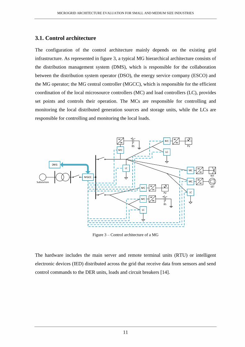
3.1. Control architecture
The configuration of the control architecture mainly depends on the existing grid
infrastructure. As represented in figure 3, a typical MG hierarchical architecture consists of
the distribution management system (DMS), which is responsible for the collaboration
between the distribution system operator (DSO), the energy service company (ESCO) and
the MG operator; the MG central controller (MGCC), which is responsible for the efficient
coordination of the local microsource controllers (MC) and load controllers (LC), provides
set points and controls their operation. The MCs are responsible for controlling and
monitoring the local distributed generation sources and storage units, while the LCs are
responsible for controlling and monitoring the local loads.
Figure 3 – Control architecture of a MG
The hardware includes the main server and remote terminal units (RTU) or intelligent
electronic devices (IED) distributed across the grid that receive data from sensors and send
control commands to the DER units, loads and circuit breakers [14].

MICROGRID ARCHITECTURE EVALUATION FOR SMALL AND MEDIUM SIZE INDUSTRIES
12
3.2. Droop control method
The droop control is implemented in the controllers of the power converters and allows
voltage and frequency control by regulating the shared active and reactive power according
to the reference set point [16]. The main idea is to emulate the operation of a typical
synchronous generator, reducing frequency as active power increases and decreasing
voltage amplitude as reactive power demand increases [20]. The formulation of the droop
equations is based on the active and reactive power shared between a bus with voltage V
and a power converter with voltage E and angle δ, as represented in figure 4.
Figure 4 – Power flow in a transmission line
The active power P and reactive power Q flowing through a transmission line with
impedance Z and angle θ can be described as [21, 22]:
𝑃 =𝑉2
𝑍∙ cos 𝜃 −
𝑉∙𝐸
𝑍∙ cos(𝜃 + 𝛿)
(1)
𝑄 =𝑉2
𝑍∙ sin 𝜃 −
𝑉∙𝐸
𝑍∙ sin(𝜃 + 𝛿)
(2)
Defining the line impedance as Z=R+jX, results in:

MICROGRID ARCHITECTURE EVALUATION FOR SMALL AND MEDIUM SIZE INDUSTRIES
13
𝑃 =𝑉
𝑋2+𝑅2 ∙ (𝑅 ∙ 𝑉 − 𝐸 ∙ cos 𝛿 + 𝑋 ∙ 𝐸 ∙ sin 𝛿)
(3)
𝑄 =𝑉
𝑋2+𝑅2 ∙ (𝑋 ∙ 𝑉 − 𝐸 ∙ cos 𝛿 − 𝑅 ∙ 𝐸 ∙ sin 𝛿)
(4)
Given that the inductance in typical transmission lines is X≫R, the resistance, R, can be
neglected:
𝑃 =𝑉∙𝐸
𝑋∙ sin 𝛿
(5)
𝑄 =𝑉2
𝑋−
𝑉∙𝐸
𝑋∙ cos 𝛿
(6)
If the power angle δ is small, then sinδ=δ and cosδ=1, resulting in the simplified
equations:
𝛿 ≅𝑋∙𝑃
𝑉∙𝐸
(7)
𝑉 − 𝐸 ≅𝑋∙𝑄
𝑉
(8)
MICROGRID ARCHITECTURE EVALUATION FOR SMALL AND MEDIUM SIZE INDUSTRIES
14
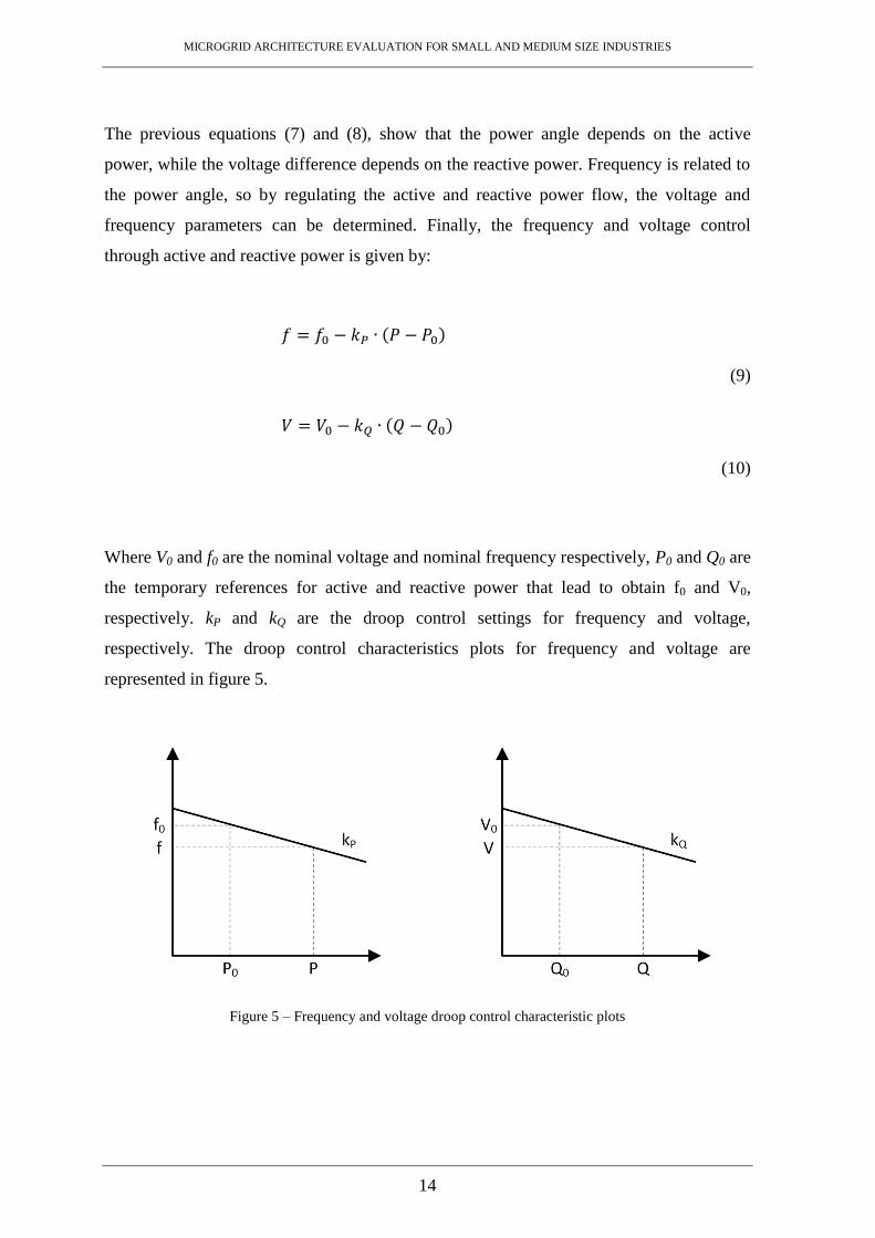
The previous equations (7) and (8), show that the power angle depends on the active
power, while the voltage difference depends on the reactive power. Frequency is related to
the power angle, so by regulating the active and reactive power flow, the voltage and
frequency parameters can be determined. Finally, the frequency and voltage control
through active and reactive power is given by:
𝑓 = 𝑓0 − 𝑘𝑃 ∙ (𝑃 − 𝑃0)
(9)
𝑉 = 𝑉0 − 𝑘𝑄 ∙ (𝑄 − 𝑄0)
(10)
Where V0 and f0 are the nominal voltage and nominal frequency respectively, P0 and Q0 are
the temporary references for active and reactive power that lead to obtain f0 and V0,
respectively. kP and kQ are the droop control settings for frequency and voltage,
respectively. The droop control characteristics plots for frequency and voltage are
represented in figure 5.
Figure 5 – Frequency and voltage droop control characteristic plots

MICROGRID ARCHITECTURE EVALUATION FOR SMALL AND MEDIUM SIZE INDUSTRIES
15
As represented in figure 5, an increase of active and reactive power will allow frequency
and voltage to decrease following a droop control setting. All the parameters are measured
and available locally, allowing frequency and voltage regulation according to the injected
active and reactive power without the need for a complex communication structure.
3.3. Hierarchical control
A hierarchical control approach consists in three distinct levels of control, as shown in
table III. A first layer of control, the primary control level, is responsible for the inner
control of the DER units and maintains the voltage and frequency. A second layer, the
secondary control level, compensates the voltage and frequency deviations caused by the
first level of control. And a third layer, the tertiary control level, manages the power flow
between the MG and the main grid according to economic concerns [23].
Table III – Hierarchical control levels
Implementation Control tasks
Primary Local Voltage and frequency maintenance through P/Q
droop control
Secondary Centralized/Decentralized Synchronization & Voltage and frequency
deviations correction
Tertiary Decentralized Power flow management & Economically optimal
grid operation
3.3.1. Primary control layer
Primary control level provides references to the inner voltage and current control loops of
the DER units based on the droop control method and stabilizes the voltage and frequency
without a communication between the power converters. The droop control applied to the
power converters emulates a synchronous generator, reducing the frequency as active
power increases. This principle is implemented in the voltage source converters using the
frequency/active power and voltage/reactive power droop control equations.

MICROGRID ARCHITECTURE EVALUATION FOR SMALL AND MEDIUM SIZE INDUSTRIES
16
𝑓 = 𝑓∗ − 𝑘𝑃 ∙ (𝑃 − 𝑃∗)
(11)
𝑉 = 𝑉∗ − 𝑘𝑄 ∙ (𝑄 − 𝑄∗)
(12)
Where f* and V* are the reference values for frequency and voltage, respectively. P* and
Q* are the references set points for the active and the reactive absorbed power.
A virtual impedance loop can also be included in the primary control level to adjust the
output impedance of the voltage source converters. The output voltage can be expressed
proportionally drooped with respect to the output current.
𝑉 = 𝑉∗ − 𝑍 ∙ 𝐼
(13)
Where V* is the voltage reference obtained by the conventional droop control equations
and Z is the virtual output impedance.
3.3.2. Secondary control layer
Secondary control level ensures that the voltage and frequency deviations are compared
with a reference value and regulated towards zero after any variation in power generation
and load change. Depending on the MGCC, this control layer can be classified in two main
types, centralized and decentralized secondary control. The correction parameters ∆f and
∆V are determined using PI compensators.
∆𝑓 = 𝐾𝑃𝑓 ∙ (𝑓∗ − 𝑓) + 𝐾𝐼𝑓 ∙ ∫(𝑓∗ − 𝑓) 𝑑𝑡
(14)

MICROGRID ARCHITECTURE EVALUATION FOR SMALL AND MEDIUM SIZE INDUSTRIES
17
∆𝑉 = 𝐾𝑃𝑉 ∙ (𝑉∗ − 𝑉) + 𝐾𝐼𝑉 ∙ ∫(𝑉∗ − 𝑉) 𝑑𝑡
(15)
Where KPf and KPV are the proportional gains, and KIf and KIV are the integral gains for
frequency and voltage respectively. The droop control equations are modified with the
correction parameters for frequency and voltage, ∆f and ∆V.
𝑓 = 𝑓∗ − 𝑘𝑃 ∙ (𝑃 − 𝑃∗) + ∆𝑓
(16)
𝑉 = 𝑉∗ − 𝑘𝑄 ∙ (𝑄 − 𝑄∗) + ∆𝑉
(17)
With a centralized secondary control approach, the control is implemented in the MGCC,
which interacts and sends references to all the local controllers. In this approach, the
voltage and frequency values are measured and compared with the references sent by the
MGCC, the resulting deviation value is then sent to the primary control in order to restore
the voltage and frequency. With a decentralized secondary approach, the control is
implemented locally on all the local controllers. In this approach the values are measured
by each local controller and sent to all the other controllers in order to determine an
average deviation to restore the voltage and frequency [24].
3.3.3. Tertiary control layer
Tertiary control level takes into account economic aspects based on real time energy prices
and manages the power flow between the MG and the main grid. The power flow is
controlled by adjusting the voltage and frequency of the DER units aiming for an
economically optimal operation for the MG. The grid active and reactive power values are

MICROGRID ARCHITECTURE EVALUATION FOR SMALL AND MEDIUM SIZE INDUSTRIES
18
measured and compared with the grid reference values P*
grid and Q*
grid in order to obtain
the frequency and voltage references f* and V*.
𝑓∗ = 𝐾𝑃𝑃 ∙ (𝑃𝑔𝑟𝑖𝑑∗ − 𝑃𝑔𝑟𝑖𝑑) + 𝐾𝐼𝑃 ∙ ∫(𝑃𝑔𝑟𝑖𝑑
∗ − 𝑃𝑔𝑟𝑖𝑑) 𝑑𝑡
(18)
𝑉∗ = K𝑃𝑄 ∙ (𝑄𝑔𝑟𝑖𝑑∗ − 𝑄𝑔𝑟𝑖𝑑) + 𝐾𝐼𝑄 ∙ ∫(𝑄𝑔𝑟𝑖𝑑
∗ − 𝑄𝑔𝑟𝑖𝑑) 𝑑𝑡
(19)
Where KPP and KPQ are the proportional gains, and KIP and KIQ are the integral gains for
the active and reactive power respectively.

MICROGRID ARCHITECTURE EVALUATION FOR SMALL AND MEDIUM SIZE INDUSTRIES
19
4. COMMUNICATION ARCHITECTURE
In order to monitor and control a system with integrated DER, power converters and
variant load patterns, an appropriated communication configuration has to be adopted. The
selection of the communication architecture for the MG depends on the existing grid
design where the control elements are located, the number of DER units, load clusters
locations, data rate, maintenance costs and mainly on the communication technology
chosen. The communication architecture can be implemented based on a centralized and
decentralized approach. With a centralized architecture (one-to-all), the central controller
coordinates the intelligent electronic devices (IED) settings for different operating
conditions. With a decentralized architecture (all-to-all), a central controller is discarded
and each IED uses the information sent from the other IEDs and coordinates the operation
settings. The local controllers are simpler in the centralized approach, since they are not in
charge of making decisions. The central controller is responsible of making decisions
based on data received from the local controllers. In the decentralized approach, each local
controller is in charge of processing data and making decisions, requiring more advanced
and complex control devices [14].
The data transmission between the power elements and IEDs and between IEDs and the
central controller can mainly follow two physical communication technologies, a wired
and a wireless communication technology. A wired communication network does not rely
on batteries to operate and generally offers higher speeds. The data transmission rate can
easily reach up to 1 Gbps or more in optical cable applications, while a wireless network
has a data transmission rate of 600 Mbps (in Wi-Fi networks), slightly less reliable and it is
more susceptible to interference. On the other hand, a wireless communication network
includes lower installation costs, easier installation of remote terminal units (RTU) and
flexibility to add new nodes to the existing network [25, 26]. Depending on the technology
adopted, the communication system can also integrate both wired and wireless links in
parallel to help reducing data traffic congestions in the wired links and improve the
availability of the network [27].

MICROGRID ARCHITECTURE EVALUATION FOR SMALL AND MEDIUM SIZE INDUSTRIES
20
4.1. Wireless communication links
There are several wireless communication technologies that are suitable for MG
communication networks, such as Wi-Fi, WiMAX, Cellular 3G/4G, ZigBee and Bluetooth
[28, 29]. These technologies may follow distinct IEEE standards and can be distinguished
by data transmission rate, operating frequency band and range as presented in table IV.
Table IV – Wireless technologies characteristics [29, 30]
Family Data rate Range Frequency
Wi-Fi
IEEE 802.11e/s up to 54 Mbps
up to 300 m 2.4 GHz / 5 GHz
IEEE 802.11n up to 600 Mbps
WiMAX IEEE 802.16 75 Mbps up to 100 km 2.5 GHz / 3.5 GHz / 5.8 GHz
WPAN
ZigBee (IEEE 802.15.4) 20 - 250 kbps up to 75 m 868 MHz / 915 MHz / 2.4
GHz
Bluetooth (IEEE 802.15.1) 1 - 3 Mbps 1 - 100 m 2.4 - 2.485 GHz
Cellular
GSM 14.4 kbps
1 - 10 km 900 - 1800 MHz
GPRS 170 kbps
3G 384 kbps – 2 Mbps
1 - 10 km
900 MHz / 2100 MHz
(or 850 MHz / 1900 MHz)
3G (HSPA)
14.4 Mbps down
5.75 Mbps up
3G (HSPA+)
84 Mbps down
22 Mbps up
up to 5 km
4G (LTE)
326 Mbps down
86 Mbps up
up to 5 km
5 - 30 km
30 - 100 km
800 MHz / 1800 MHz / 2600
MHz
(or 700 MHz / 1700 MHz /
1900 MHz) 4G (LTE Advanced)
1 Gbps down
500 Mbps up
4.1.1. Wi-Fi
A Wi-Fi network provides a flexible, reliable and high speed local wireless communication
based on the IEEE 802.11x standards. Wi-Fi 802.11e and 802.11s standard specifications
propose the implementation of the wireless home and local area network (WLAN) on the
2.4 GHz / 5 GHz frequency bands, offering 54 Mbps data transmission speed and range up
MICROGRID ARCHITECTURE EVALUATION FOR SMALL AND MEDIUM SIZE INDUSTRIES
21
to 300 m. Wi-Fi 802.11n standard specifications propose implementations on the 2.4 GHz /
5 GHz frequency bands up to 300 m with data rates of 600 Mbps. Because Wi-Fi networks
operate on the unlicensed spectrum, their deployment is relatively cheap. But at the same
time, the use of a crowded unlicensed spectrum also makes Wi-Fi networks more
susceptible to interference [29].
4.1.2. WiMAX
A WiMAX network offers a long coverage area and high speed wireless communication
based on the IEEE 802.16x standards. WiMAX 802.16 standard specifications define
implementation on the 2.5 GHz / 3.5 GHz / 5.8 GHz frequency bands with data
transmission speeds of 75 Mbps. It also proposes a coverage area up to a maximum of 100
kms depending on the performance. Other WiMAX IEEE standards allow implementation
on higher frequency bands with lower data rates. However, high spectrum frequencies
cannot support non-line-of-sight (NLOS) transmission scenarios, requiring a line-of-sight
(LOS) scenario to operate, where a path between the receiver and transmitter is visible.
WiMAX provides good performance over long distances and supports thousands of
simultaneous users. However, a WiMAX network requires a complex network
management [29].
4.1.3. ZigBee
A ZigBee network provides a low power and low cost local wireless communication based
on the IEEE 802.15.4 standards. It proposes a worldwide use on the 2.4 GHz frequency
band (Europe – 868 MHz and North America – 915 MHz) and a typical range up to 75 m
with low data rates of 20-250 kbps. The ZigBee Pro supports an increased coverage area
up to 1600 m [30]. ZigBee is considered an ideal network for energy metering and
management applications that require both low power consumption and low bandwidth
with a low deployment cost [31]. This technology offers a simple and cheap solution,
making it the most adopted technology for wireless personal area networks (WPAN) in
commercial and industrial applications [29].

MICROGRID ARCHITECTURE EVALUATION FOR SMALL AND MEDIUM SIZE INDUSTRIES
22
4.1.4. Bluetooth
A Bluetooth network provides a low power local wireless communication with low
deployment costs based on the IEEE 802.15.1 standards. It operates on the 2.4-2.485 GHz
frequency band with a data transmission speed of 1-3 Mbps and a coverage area of 1-100
m. Bluetooth networks offers less latency than ZigBee or Wi-Fi networks and can be often
used in local monitoring applications [28, 32]. Due to the limited range, both Bluetooth
and ZigBee networks are unable to scale to large networks [29]. This technology suffers
from security concerns, but it is still widely adopted for wireless personal area networks
(WPAN) with low cost deployment.
4.1.5. Cellular 3G/4G
The 3rd Generation (3G) and 4th Generation (4G) cellular networks provide long distance
wireless communications with ranges up to 10 km and 100 km, respectively. Cellular 3G
operates on the 900 MHz / 2100 MHz frequency band (or 850 MHz / 1900 MHz) with a
coverage area of 1-10 km and data rates of 384 kbps to 2 Mbps. 3G (HSPA) offers data
download speeds of 14.4 Mbps and data upload speeds of 5.75 Mbps with ranges up to 10
km. 3G (HSPA+) offers an increased data download speed of 84 Mbps and a data upload
speed of 22 Mbps with a lower coverage area up to 5 km. Cellular 4G operates on the 800
MHz / 1800 MHz / 2600 MHz frequency band (or 700 MHz / 1700 MHz / 1900 MHz)
with an extended range up to 100 km with a performance hit. The optimum and acceptable
operation of cellular 4G is at ranges up to 5 km and 5-30 km, respectively. The operation
over longer distances up to 100 km has a reduced performance. 4G (LTE) provides a data
download speed of 326 Mbps and a data upload speed of 86 Mbps. 4G (LTE Advanced)
offers a much higher data download speed of 1 Gbps and data upload speed of 500 Mbps.
The low power consumption of terminal equipment and an extensive data coverage area
with high flexibility are the main advantages of cellular networks [29]. Furthermore, public
cellular networks are already deployed and can be used with no maintenance costs [28].
However, there are high costs associated with the use of a service provider network and
there is no guarantee of service during abnormal weather conditions [31].

MICROGRID ARCHITECTURE EVALUATION FOR SMALL AND MEDIUM SIZE INDUSTRIES
23
4.2. Wired communication links
The MG communication network may also be integrated with physical wired
communication links such as PLC, DSL and optical fibre [29, 33]. The wired technologies
follow different IEEE and ITU standards and are distinguished by data transmission rate,
operating frequency band and range as presented in table V.
Table V – Wired technologies characteristics [29, 30]
Family Data rate Range Frequency
PLC
NB-PLC (ITU-T G.hnem, IEEE
1901.2) up to 500 kbps +150 km 3 - 500 kHz
BB-PLC (ITU-T G.hn, IEEE
1901) up to 10 Mbps up to 1.5 km 1.8 - 250 MHz
Optical
fibre
AON (IEEE 802.3ah) 100 Mbps up to 10 km
500 MHz*km PON (BPON (ITU-T G.983),
GPON (ITU-T G.984), EPON
(IEEE 802.3ah))
155 - 2448 Mbps 10 - 60 km
xDSL
HDSL (ITU G.991.1) 2 Mbps up to 3.6 km 0.1 - 292 kHz
ADSL (ITU G.992.1)
8 Mbps down
1.3 Mbps up
up to 4 km
25 kHz – 1.1 MHz
ADSL2 (ITU G.992.3)
12 Mbps down
3.5 Mbps up
up to 7 km
ADSL2+ (ITU G.992.5)
24 Mbps down
3.3 Mbps up
25 kHz – 2.2 MHz
VDSL (ITU G.993.1)
52 - 85 Mbps down
16 - 85 Mbps up
up to 1.2 km
25 kHz – 12 MHz
VDSL2 (ITU G.993.1) up to 200 Mbps 300 m – 1.5 km
4.2.1. PLC
Power line communications (PLC) makes use of existing power lines for data
communication. A PLC network provides a cost-effective solution with a low maintenance
requirement, since a single infrastructure is used for both data and power transmission
[29]. The narrowband PLC (NB-PLC) is based on the ITU-T G.hnem and IEEE 1901.2

MICROGRID ARCHITECTURE EVALUATION FOR SMALL AND MEDIUM SIZE INDUSTRIES
24
standards that define a data transmission speed up to 500 kbps on the 3-500 KHz frequency
band and a coverage area of 150 km or more. The broadband PLC (BB-PLC) is based on
the ITU-T G.hn and IEEE 1901 standards that define a higher data transmission speed up
to 10 Mbps on the 1.8-250 MHz with a shorter coverage area up to 1.5 km. BB-PLC is also
capable of providing data rates up to 200 Mbps in very short distances by operating on
higher frequency bands. Because PLC makes use of a single infrastructure for data and
power decreasing the cost of installation, this communication technology is the preferred
solution for metering data transmission and the simplest to implement in smart grid
applications. However, the noisy and harsh nature of the power line channel affects the
data transmission and may decrease the quality of signal [31].
4.2.2. Optical fibre
An optical fibre infrastructure provides long distance communication with high data rates
with robustness against radio and electromagnetic interferences. However, optical fibre
applications are characterized by high installation costs, high terminal equipment costs and
difficulty to upgrade. These disadvantages prevent optical fibre communications from
being widely adopted in smart grids [29]. Active optical network (AON) is based on the
IEEE 802.3ah standard and offers data transmission speeds of 100 Mbps with a range up to
10 km. AON requires electrically powered switching equipment such as routers or a switch
aggregator to manage signal distribution and direct signals to the correct destination.
Passive optical network (PON) technologies provide higher data transmission speeds of
155-2448 Mbps with ranges from 10 km to 60 km, depending on the standard used. PON
does not require electrically powered switching equipment, instead it uses optical splitters
to separate and collect the signals. Optical fibre applications operate on the 500 MHz
frequency band for distances of 1 km (500 MHz*km).
4.2.3. DSL
Digital subscriber lines (DSL) uses telephone line infrastructures to transmit digital data.
This avoids additional communication infrastructures when a telephone line infrastructure
is already deployed [29]. High-bit-rate DSL (HDSL) is based on the ITU G.991.1 and
MICROGRID ARCHITECTURE EVALUATION FOR SMALL AND MEDIUM SIZE INDUSTRIES
25
supports data transmission rates up to 2 Mbps on the 0.1-292 kHz frequency band and a
maximum coverage of 3.6 km. Asymmetric DSL (ADSL) is based on the ITU G.992.1 and
provides a data download speed of 8 Mbps and a data upload speed of 1.3 Mbps on the 25
kHz to 1.1 MHz frequency bands with a coverage area up to 4 km. Asymmetric DSL
version 2 (ADSL2) is based on the ITU G.992.3 and provides a higher data download
speed of 12 Mbps and a higher data upload speed of 3.5 Mbps on the 25 kHz to 1.1 MHz
frequency bands with an increased coverage area up to 7 km. Asymmetric DSL version 2
plus (ADSL2+) is based on the ITU G.992.5 and provides increased data download speed
of 24 Mbps and a slightly lower data upload speed of 3.3 Mbps on the 25 kHz to 2.2 MHz
frequency bands with a coverage area up to 7 km. Very-high-bit-rate DSL (VDSL) is based
on the ITU G.993.1 and supports an increased data download speed of 52-85 Mbps and
data upload speed of 16-85 Mbps on the 25 kHz to 12 MHz frequency bands with reduced
maximum coverage of 1.2 km. Very-high-bit-rate DSL version 2 (VDSL2) supports data
transmission speeds up to 200 Mbps with a typical range from 300 m to 1.5 km. In order to
use DSL networks, a communication fee must be paid to the telecommunication operator
and the network needs to be regularly maintained [29, 31].
4.3. Communication protocols and standards
The Internet protocol suite (TCP/IP) is a set of communication protocols organized into
four distinct layers [27]. The application layer is the highest layer and provides protocols
that enable process-to-process data communication. Some of the protocols can be
Hypertext Transfer Protocol (HTTP), Secure Shell (SSH), Network Timing Protocol
(NTP), Distributed Network Protocol (DNP3) and Modbus. The transport layer establishes
data channels and provides host-to-host data communication through protocols such as
Transmission Control Protocol (TCP) and User Datagram Protocol (UDP). The internet
layer provides authentication and defines the addressing and routing structures through
internet protocols IPv4 and IPv6. The link layer is the lowest layer and defines methods for
the local network communication link. Table VI shows the protocols for each layer of the
TCP/IP model.

MICROGRID ARCHITECTURE EVALUATION FOR SMALL AND MEDIUM SIZE INDUSTRIES
26
Table VI – TCP/IP model layers
Layer Protocols Function
1 Application HTTP, SSH, NTP Enables process-to-process
data communication
2 Transport TCP, UDP Provides host-to-host data
communication
3 Internet IPv4, IPv6 Defines the addressing and
routing structures
4 Link Serial, Ethernet Defines methods for
communication link
4.3.1. Modbus
Modbus is a communication protocol that enables communication between a server unit
and clients connected to the same network. It is often used in supervisory control and data
acquisition (SCADA) systems for a robust communication between supervisory units and
remote terminal units (RTU). In a MG with Modbus protocol model, the central controller
may act as a server while each IED acts as a client. The data communication between the
server and clients is made based on polls from the server. Modbus can be transmitted over
RS232, RS485 and Ethernet (TCP/IP) using protocol converters.
4.3.2. DNP3
DNP3 is a new communication protocol often used for data acquisition in SCADA systems
that provides a reliable and efficient server to client data communication. Unlike the older
protocol Modbus, DNP3 allows client units to be updated without waiting for a poll from
the server and supports time synchronization with RTUs by including timestamp variants.
DNP3 offers a robust communication and compatibility with a wide range of equipment,
being widely used in several industrial applications.

MICROGRID ARCHITECTURE EVALUATION FOR SMALL AND MEDIUM SIZE INDUSTRIES
27
4.3.3. IEC 61850
IEC 61850 is a communication standard that defines data models, events and settings for
substation IED configurations. These data models can be mapped to a number of protocols,
such as Manufacturing Message Specification (MMS), Generic Object Oriented Substation
Event (GOOSE) and Sampled Measured Values (SMV). The IEC 61850 standard enables
the integration of protection, control and measurement functions in substation applications.


MICROGRID ARCHITECTURE EVALUATION FOR SMALL AND MEDIUM SIZE INDUSTRIES
29
5. MICROGRID ARCHITECTURE
The implementation of low-carbon energy sources into the power grid is an approach that
has been made in order to reduce GHG and carbon emissions in the power sector. This
environmental effort led to several MG architecture configurations with high penetration of
RES [34].
This section presents a basic architecture of a MG and its DG units, storage units and
loads. The main purpose of this architecture is to introduce different technologies for the
most common energy resources in MGs. The characteristics for these energy resources are
summarized in Appendix A. As represented in figure 6, this architecture consists of a
HV/MV transformer substation (T1), MV/LV transformers (T2 and T3), groups of
distributed generation (G1 and G2) and load clusters (L1 and L2).
Figure 6 – Basic microgrid architecture
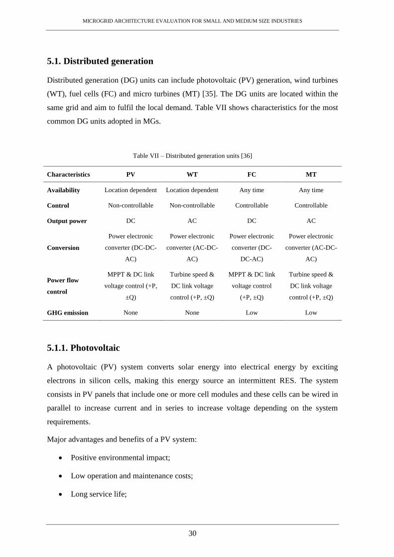
MICROGRID ARCHITECTURE EVALUATION FOR SMALL AND MEDIUM SIZE INDUSTRIES
30
5.1. Distributed generation
Distributed generation (DG) units can include photovoltaic (PV) generation, wind turbines
(WT), fuel cells (FC) and micro turbines (MT) [35]. The DG units are located within the
same grid and aim to fulfil the local demand. Table VII shows characteristics for the most
common DG units adopted in MGs.
Table VII – Distributed generation units [36]
Characteristics PV WT FC MT
Availability Location dependent Location dependent Any time Any time
Control Non-controllable Non-controllable Controllable Controllable
Output power DC AC DC AC
Conversion
Power electronic
converter (DC-DC-
AC)
Power electronic
converter (AC-DC-
AC)
Power electronic
converter (DC-
DC-AC)
Power electronic
converter (AC-DC-
AC)
Power flow
control
MPPT & DC link
voltage control (+P,
±Q)
Turbine speed &
DC link voltage
control (+P, ±Q)
MPPT & DC link
voltage control
(+P, ±Q)
Turbine speed &
DC link voltage
control (+P, ±Q)
GHG emission None None Low Low
5.1.1. Photovoltaic
A photovoltaic (PV) system converts solar energy into electrical energy by exciting
electrons in silicon cells, making this energy source an intermittent RES. The system
consists in PV panels that include one or more cell modules and these cells can be wired in
parallel to increase current and in series to increase voltage depending on the system
requirements.
Major advantages and benefits of a PV system:
Positive environmental impact;
Low operation and maintenance costs;
Long service life;

MICROGRID ARCHITECTURE EVALUATION FOR SMALL AND MEDIUM SIZE INDUSTRIES
31
Clean and silent operation;
Generation coincides with peak energy demand.
This solution also brings some disadvantages such as high fixed costs, low cell efficiency,
location restrictions and weather dependent. A common way to overcome these
disadvantages is to integrate the PV systems with other energy resources.
Solar cells made from crystalline silicon (c-Si) are generally the most common and
efficient ones. Depending on the alignment of the silicon molecules and manufacturing
process, silicon cells can be made from a single pure crystal of silicon, called
monocrystalline (mono-Si) cells and made from an ingot of melted and recrystallized
silicon, called polycrystalline (poly-Si) cells. Solar cells can also be made by depositing
thin layers of non-crystallized silicon onto a substrate, forming thin-film amorphous (a-Si)
cells. Monocrystalline PV panels have the longest service life and also the highest
efficiency rates and power output with the least amount of required space. Due to the
complicated manufacturing process and purity of the monocrystalline cells,
monocrystalline PV panels have the highest production costs and a significant amount of
silicon results in waste. Although performance decreases with temperature,
monocrystalline technology has a better heat tolerance in warm weather. Polycrystalline
PV panels have a slightly lower efficiency and heat tolerance, but the manufacturing
process is simpler and costs less, resulting in cheaper panels. Amorphous PV panels are the
cheapest to manufacture and can be produced with a flexible substrate, but this technology
has the lowest power output and efficiency rates. The typical efficiency rates are around
15% to 23% for monocrystalline PV panels, 13% to 16% for polycrystalline PV panels and
5% to 10% for amorphous PV panels [37]. Table VIII shows the highest confirmed module
efficiencies independently measured by a test centre [38].
Table VIII – Solar modules efficiencies [38]
Technology Efficiency (%) Area (cm2) Voc (V) Isc (A) Fill Factor (%)
Crystalline silicon
Monocrystalline silicon 24.4 ± 0.5
13177 (da) 79.5 5.04 80.1
Polycrystalline silicon 19.9 ± 0.4 15143 (ap) 78.87 4.795 79.5

MICROGRID ARCHITECTURE EVALUATION FOR SMALL AND MEDIUM SIZE INDUSTRIES
32
Thin-film
Amorphous silicon 12.3 ± 0.3 14322 (t) 280.1 0.902 69.9
(t) – Total area
(ap) – Aperture area (masked)
(da) – Designated area (masked)
Standard Test Conditions (STC) - Irradiance: 1000 W/m2; Spectrum: AM 1.5; Temperature: 25°C
Table IX shows the comparison between two solar modules, a monocrystalline module and
a polycrystalline module as shown in figures 7a) and 7b). Both solar modules are from
Trina Solar, which is one of the top ranked solar panel manufacturers. These PV modules
are meant for utility applications and they are equal in size and number of cells.
Table IX – Trina Solar modules comparison [39]
Module
DUOMAX M+
Dual glass 72 cell TSM-DEG14 (II)
DUOMAX
Dual glass 72 cell TSM-PEG14
Solar cells
Monocrystalline
(156.75 x 156.75 mm)
Polycrystalline
(156.75 x 156.75 mm)
Cell orientation
72 cells
(6 x 12)
72 cells
(6 x 12)
Peak power range
(STC) 335 – 365 Wp 320 – 335 Wp
Maximum power
voltage (STC) 37.9 – 39.1 V 37.2 – 37.8 V
Maximum power
current (STC) 8.84 – 9.35 A 8.60 – 8.87 A
Module efficiency
(STC) 17.1 – 18.6 % 16.3 – 17.1 %
Standard Test Conditions (STC) - Irradiance: 1000 W/m2; Spectrum: AM 1.5; Temperature: 25°C

MICROGRID ARCHITECTURE EVALUATION FOR SMALL AND MEDIUM SIZE INDUSTRIES
33
a) b)
Figure 7 – Types of solar cell modules [39]: a) Monocrystalline and b) Polycrystalline
Including solar trackers in PV panels is a common adopted solution to maximize the
production of the PV system. Solar tracker devices keep the PV panels oriented towards
the sun throughout the day in order to minimize the angle of incidence. The power output
is maximized when the angle of incidence is close to 0°, meaning that the light rays have to
strike perpendicularly to the PV surface. Solar trackers are categorized as single-axis and
dual-axis trackers. Single-axis trackers follow the sun rotating on a single horizontal or
vertical axis. The horizontal axis type is used in tropical regions where the position of the
sun during noon is usually high. The vertical axis type is generally used in high latitude
regions where the position of the sun is not very high. Dual-axis trackers point directly at
the sun, moving vertically and horizontally on two axes. The dual-axis solar trackers can
be used effectively anywhere in the world [40].
Depending on the geographic location, solar trackers generally offer an increase of 10% to
40% in annual output power over fixed systems [40, 41]. In addition, solar tracker PV
systems are able to generate more electricity in the same amount of space needed for
stationary PV systems, making tracker units more space efficient than fixed units.
However, a solar tracker PV system is more expensive than a stationary PV unit and there
is an extra maintenance requirement associated with the additional moving parts. Both
stationary and solar tracker PV systems are shown in figures 8a) and 8b).

MICROGRID ARCHITECTURE EVALUATION FOR SMALL AND MEDIUM SIZE INDUSTRIES
34
a) b)
Figure 8 – PV systems: a) Fixed [42] and b) Solar tracker [43]
The capital cost estimates of grid-tie DG technologies for residential, commercial and
industrial facilities are given in dollars per installed kilowatt of the generating capacity
($/kW). The installed cost of PV systems has been through a substantially decrease due to
increased competition in the PV manufacturing industry. According to the cost data
provided by the National Renewable Energy Laboratory (NREL), recent installed costs
vary from 3000 $/kWp to 4800 $/kWp for PV systems below 10 kWp, between 2500
$/kWp to 4500 $/kWp for 10-100 kWp PV systems and around 1700 $/kWp to 3300
$/kWp for larger 100-1000 kWp PV systems [44].
5.1.2. Wind turbine
A wind turbine (WT) system converts wind energy into electrical energy by using the wind
force to turn the blades and make a rotor spin, being also an intermittent RES. The main
parts of a WT are the tower, rotor and nacelle. The nacelle contains the brake, gearbox to
increase rotational speed (turbines with output power greater than 10 kW) and the
generator that is connected to the rotor by the main shaft.
Depending on the rotor orientation, WTs may have vertical axis or horizontal axis
configuration as shown in figures 9a) and 9b). Horizontal axis wind turbines (HAWT) have
the main rotor shaft, generator and other components on top of a tall tower, the main rotor
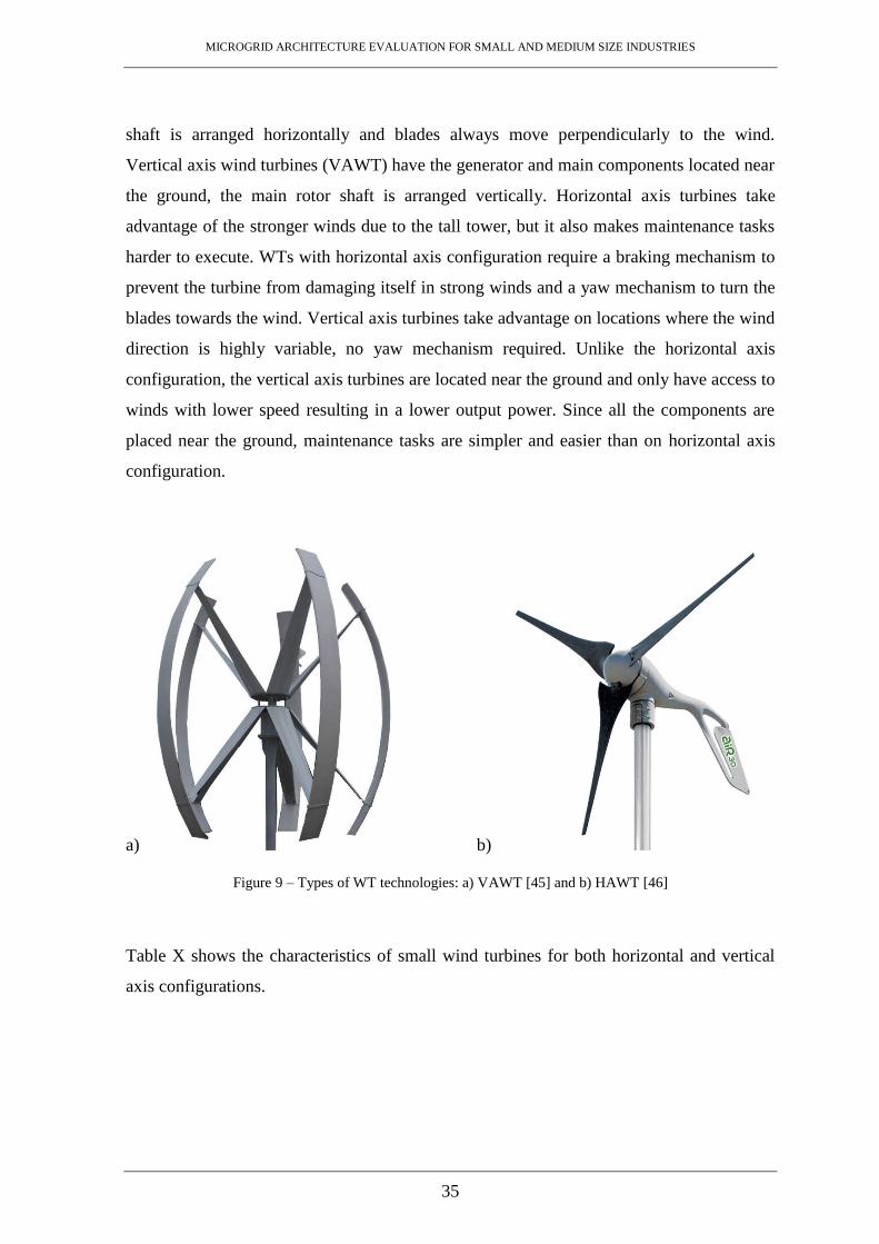
MICROGRID ARCHITECTURE EVALUATION FOR SMALL AND MEDIUM SIZE INDUSTRIES
35
shaft is arranged horizontally and blades always move perpendicularly to the wind.
Vertical axis wind turbines (VAWT) have the generator and main components located near
the ground, the main rotor shaft is arranged vertically. Horizontal axis turbines take
advantage of the stronger winds due to the tall tower, but it also makes maintenance tasks
harder to execute. WTs with horizontal axis configuration require a braking mechanism to
prevent the turbine from damaging itself in strong winds and a yaw mechanism to turn the
blades towards the wind. Vertical axis turbines take advantage on locations where the wind
direction is highly variable, no yaw mechanism required. Unlike the horizontal axis
configuration, the vertical axis turbines are located near the ground and only have access to
winds with lower speed resulting in a lower output power. Since all the components are
placed near the ground, maintenance tasks are simpler and easier than on horizontal axis
configuration.
a) b)
Figure 9 – Types of WT technologies: a) VAWT [45] and b) HAWT [46]
Table X shows the characteristics of small wind turbines for both horizontal and vertical
axis configurations.

MICROGRID ARCHITECTURE EVALUATION FOR SMALL AND MEDIUM SIZE INDUSTRIES
36
Table X – Small wind turbine characteristics [44, 47, 48]
Technology Efficiency Power $/kW Noise Wind
resistance
Starting
wind speed
HAWT 20 to 50%
Up to 100
kW
4000 - 8500 (10
- 100 kW) 5 - 60dB Weak 2.5 - 5 m/s
VAWT 20 to 40% Up to 100
kW
4000 - 8500 (10
- 100 kW) 0 - 10dB Strong 1.5 - 3 m/s
5.1.3. Fuel cell
A fuel cell (FC) system converts chemical energy from a fuel into electrical energy through
a chemical reaction of positive charged hydrogen ions with an oxidizer such as oxygen. A
fuel cell consists of two electrodes and an electrolyte that allows the particles to move
between them, the positive electrode is called cathode and the negative is called anode.
The two most common FC technologies for domestic and small scale industrial
applications are the proton exchange membrane fuel cells (PEMFC) and solid oxide fuel
cells (SOFC). PEMFC operate at low temperatures (80°C) with a polymer electrolyte and
use platinum for both electrodes, resulting in higher manufacturing costs. These fuel cells
can be used on both portable and stationary applications due to their light weight and
compact characteristics. This technology offers fast start capability and rapid response
times to load changes. SOFC normally use an yttria-stabilized zirconia (YSZ) electrolyte
and operate at high temperatures (around 800°C) enabling any fuel containing hydrogen to
be used. Due to the high operating temperature, this technology is well suited for combined
heat and power (CHP) applications. Unlike PEMFC, the SOFC are only intended for
stationary applications due to their heavy weight and low tolerance for vibrations and
frequency stops. Larger scale industrial and commercial applications may use other types
of FCs such as molten carbonate fuel cells (MCFC) and phosphoric acid fuel cells (PAFC).
MCFC operate at high temperatures (around 650°C) and use a molten carbonate salt
suspended in a porous ceramic matrix as the electrolyte. The high temperatures enable non-
noble metals to be used as catalysts at the anode and cathode. PAFC use phosphoric acid as
the electrolyte and operate at moderate temperatures (around 190°C). Platinum is used as
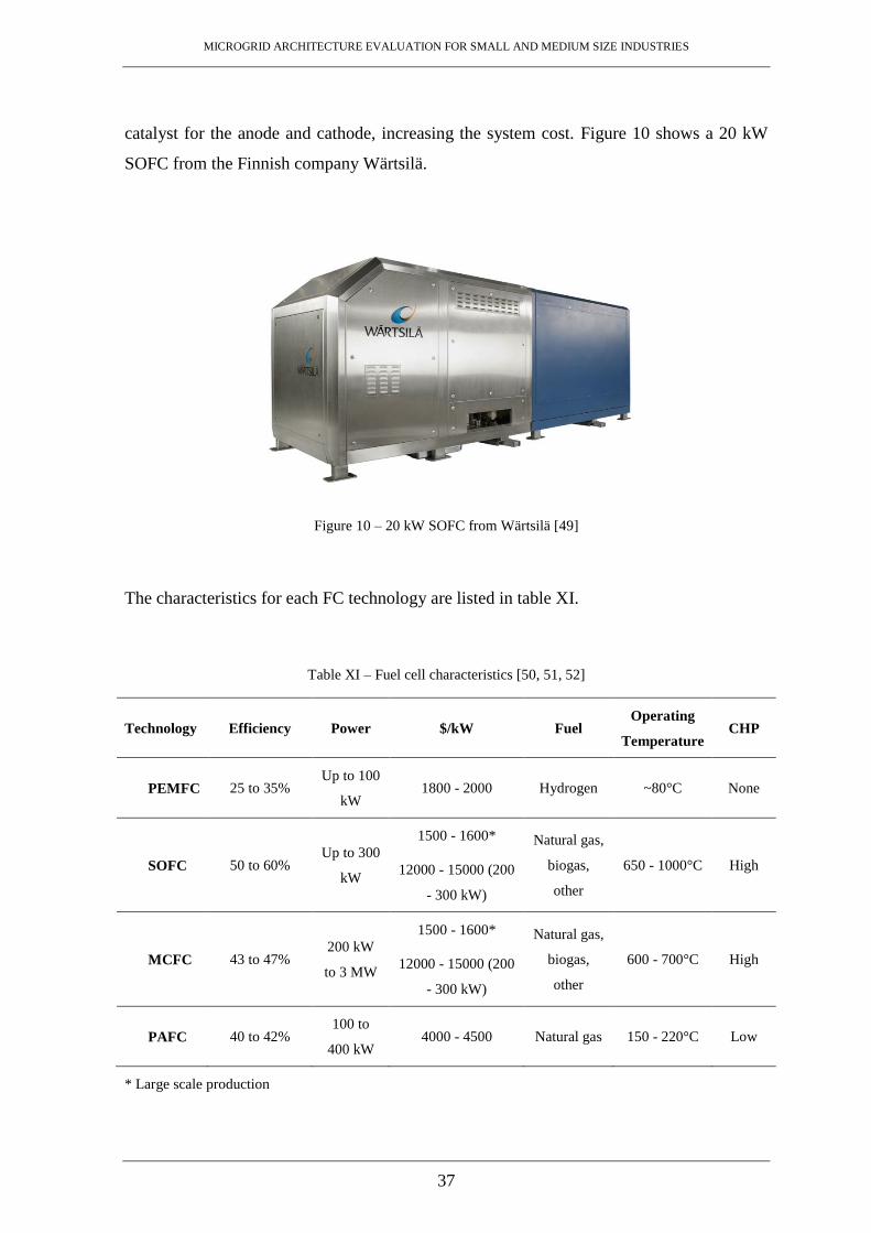
MICROGRID ARCHITECTURE EVALUATION FOR SMALL AND MEDIUM SIZE INDUSTRIES
37
catalyst for the anode and cathode, increasing the system cost. Figure 10 shows a 20 kW
SOFC from the Finnish company Wärtsilä.
Figure 10 – 20 kW SOFC from Wärtsilä [49]
The characteristics for each FC technology are listed in table XI.
Table XI – Fuel cell characteristics [50, 51, 52]
Technology Efficiency Power $/kW Fuel Operating
Temperature CHP
PEMFC 25 to 35%
Up to 100
kW 1800 - 2000 Hydrogen ~80°C None
SOFC 50 to 60% Up to 300
kW
1500 - 1600*
12000 - 15000 (200
- 300 kW)
Natural gas,
biogas,
other
650 - 1000°C High
MCFC 43 to 47% 200 kW
to 3 MW
1500 - 1600*
12000 - 15000 (200
- 300 kW)
Natural gas,
biogas,
other
600 - 700°C High
PAFC 40 to 42% 100 to
400 kW 4000 - 4500 Natural gas 150 - 220°C Low
* Large scale production
MICROGRID ARCHITECTURE EVALUATION FOR SMALL AND MEDIUM SIZE INDUSTRIES
38
5.1.4. Micro turbine
A micro turbine (MT) system produces heat and electricity from a combustion turbine. The
basic components of a MT are the compressor-turbine package mounted on a shaft along
with the generator and the recuperator that uses the turbine exhaust heat to preheat the
compressed air. The exhaust heat can be recovered by the heat exchanger package and
used in CHP applications.
The MTs used for power generation can be single cycle or recuperated micro turbines. In a
recuperated turbine, the recovered heat stream from the exhaust is sent back to the
incoming air stream in order to boost the temperature of the air stream supplied to the
combustor and some of the exhaust heat can be used in CHP applications. Due to preheat,
recuperated turbines can save up to around 40% of fuel consumption. In a single cycle
turbine, the compressed air is mixed with fuel and burned under constant pressure
conditions, resulting hot gas that expands through a turbine. All the exhaust heat can be
used in CHP applications, unlikely recuperated turbines that use part of that heat for
preheating. Depending on the shaft configuration, MTs can also be classified as single
shaft or split shaft micro turbines. In single shaft turbine configurations, all the rotating
parts such as compressor, turbine and generator share a common shaft. These turbines
usually operate at high speeds (50000 to 120000 rpm) and can be used in applications with
constant load changes. In a split shaft turbine configuration, the rotating parts such as
compressor and generator are not integrated within the same shaft. The compressor is
driven by a compressor turbine and the generator is driven by a power turbine. These
turbines operate at lower speeds and offer slower response times to load changes. Figure
11 shows a 200 kW MT module from Capstone.

MICROGRID ARCHITECTURE EVALUATION FOR SMALL AND MEDIUM SIZE INDUSTRIES
39
Figure 11 – 200 kW MT module from Capstone [53]
The characteristics for typical MTs are listed in table XII.
Table XII – Microturbine characteristics [54]
Efficiency Power $/kW Heat rate CHP
25 to 30%
(80% w/ heat recovery)
30 kW to 1
MW 500 - 3000
10000 to 13000
Btu/kWh High
5.2. Energy storage
Energy storage units can include battery storage (BS), flywheel (FW) systems and even
supercapacitors (SC) [35]. The storage elements presented in table XIII are included to
ensure an uninterrupted supply of power during outages and to set a power balance after
significant load changes. Storage applications can be classified as centralized units and
decentralized units. Centralized units are normally installed at transformer substations, this
type of storage serves power balance and frequency regulation aims. Decentralized units
are normally dispersed over the whole grid, close to loads and generation sources, serving
demand response aims.
MICROGRID ARCHITECTURE EVALUATION FOR SMALL AND MEDIUM SIZE INDUSTRIES
40
Table XIII – Storage units [36]
Characteristics BS FW SC
Storage duration Long-term storage Short-term storage Short-term storage
Output power DC AC DC
Conversion Power electronic
converter (DC-DC-AC)
Power electronic
converter (AC-DC-AC)
Power electronic converter
(DC-DC-AC)
Power flow control
State of charge &
voltage/frequency
control (+P,±Q)
Speed control (±P,±Q) State of charge control
(±P,±Q)
GHG emission None None None
5.2.1. Battery storage
A battery storage (BS) system stores energy in chemical form and converts the stored
chemical energy back to electricity when needed. A battery consists of an electrolyte and
two electrodes, the cathode (positive electrode) and anode (negative electrode). In large
scale energy storage applications, a group of batteries is joined in parallel for a current
increase or in series for voltage increase, forming a battery bank to supply the local loads.
Controllers are necessary to prevent the batteries from overcharging.
Most industrial energy storage applications are mainly focused on lithium ion (Li-ion),
nickel metal hydride (NiMH) and lead acid (Pb-A) battery technologies. Lithium ion
batteries use lithiated metal oxide for the negative electrode and graphitic carbon for the
positive electrode, the electrolyte consists of lithium salts in organic carbonates. Generally,
these batteries have the best performance, but suffer from safety concerns and high system
costs. Lithium is used as electrode material, which is highly reactive, resulting in a high
energy density (exceeding 150 Wh/kg) and efficient charging. Nickel metal hydride
batteries use metal hydride for the negative electrode and nickel hydroxide for the positive
electrode, the alkaline electrolyte often consists of potassium hydroxide. These batteries
offer good performance with a relatively safe and durable operation, but with a high
system cost and maintenance requirement. Lead acid batteries consist of lead metal and
lead dioxide electrodes immersed in sulphuric acid. They have a slow and inefficient
charging, but this technology offers a cheap and mature solution. The lead and sulphuric

MICROGRID ARCHITECTURE EVALUATION FOR SMALL AND MEDIUM SIZE INDUSTRIES
41
acid contained within the batteries can be a health hazard and cause environmental
impacts, which prevent lead acid batteries from being a widely adoption. Figure 12 shows
batteries forming a battery bank.
Figure 12 – Battery bank [55]
The characteristics for the most common battery technologies are listed in table XIV.
Table XIV – Battery storage characteristics [56, 57, 58]
Technology Efficiency Capacity Power Wh/kg $/kWh $/kW Cycles
Li-ion 75 to 90%
Up to 50
MWh
Up to 50
MW 90 - 190 600 - 2500
1200 -
4000 ~3000
Pb-A 70 to 90% Up to 40
MWh
Up to 20
MW 40 200 - 400 300 - 600 500 - 2000
Ni-
based 72 to 78%
Up to 20
MWh
Up to 50
MW 50 800 - 1500
500 -
1500 1500 - 3000
5.2.2. Flywheel
A flywheel (FW) system stores mechanical energy in a spinning shaft connected to a
generator, the rotor spins building up kinetic energy and converts it to electricity when
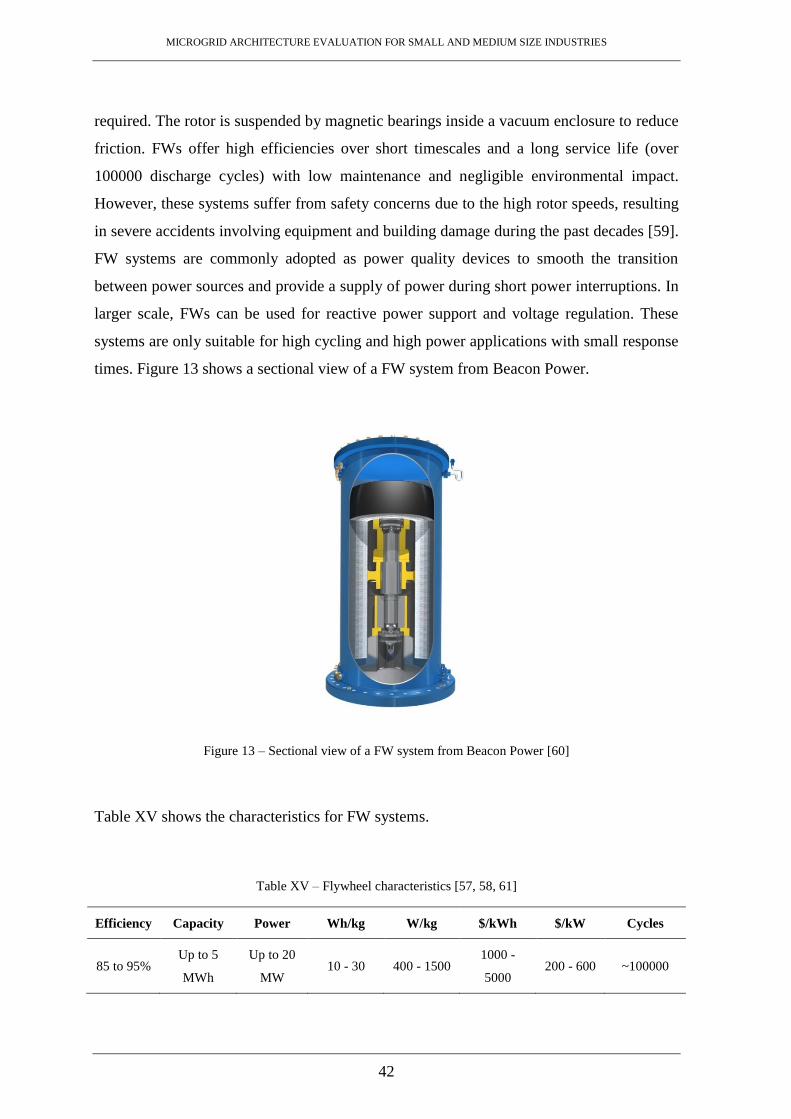
MICROGRID ARCHITECTURE EVALUATION FOR SMALL AND MEDIUM SIZE INDUSTRIES
42
required. The rotor is suspended by magnetic bearings inside a vacuum enclosure to reduce
friction. FWs offer high efficiencies over short timescales and a long service life (over
100000 discharge cycles) with low maintenance and negligible environmental impact.
However, these systems suffer from safety concerns due to the high rotor speeds, resulting
in severe accidents involving equipment and building damage during the past decades [59].
FW systems are commonly adopted as power quality devices to smooth the transition
between power sources and provide a supply of power during short power interruptions. In
larger scale, FWs can be used for reactive power support and voltage regulation. These
systems are only suitable for high cycling and high power applications with small response
times. Figure 13 shows a sectional view of a FW system from Beacon Power.
Figure 13 – Sectional view of a FW system from Beacon Power [60]
Table XV shows the characteristics for FW systems.
Table XV – Flywheel characteristics [57, 58, 61]
Efficiency Capacity Power Wh/kg W/kg $/kWh $/kW Cycles
85 to 95%
Up to 5
MWh
Up to 20
MW 10 - 30 400 - 1500
1000 -
5000 200 - 600 ~100000
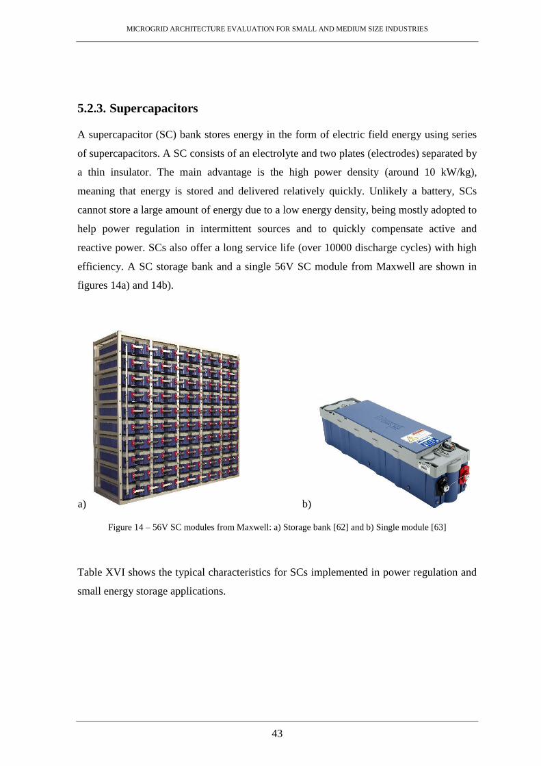
MICROGRID ARCHITECTURE EVALUATION FOR SMALL AND MEDIUM SIZE INDUSTRIES
43
5.2.3. Supercapacitors
A supercapacitor (SC) bank stores energy in the form of electric field energy using series
of supercapacitors. A SC consists of an electrolyte and two plates (electrodes) separated by
a thin insulator. The main advantage is the high power density (around 10 kW/kg),
meaning that energy is stored and delivered relatively quickly. Unlikely a battery, SCs
cannot store a large amount of energy due to a low energy density, being mostly adopted to
help power regulation in intermittent sources and to quickly compensate active and
reactive power. SCs also offer a long service life (over 10000 discharge cycles) with high
efficiency. A SC storage bank and a single 56V SC module from Maxwell are shown in
figures 14a) and 14b).
a) b)
Figure 14 – 56V SC modules from Maxwell: a) Storage bank [62] and b) Single module [63]
Table XVI shows the typical characteristics for SCs implemented in power regulation and
small energy storage applications.

MICROGRID ARCHITECTURE EVALUATION FOR SMALL AND MEDIUM SIZE INDUSTRIES
44
Table XVI – Supercapacitor characteristics [57, 58, 61]
Efficiency Capacity Power Wh/kg W/kg $/kWh $/kW Cycles
90 to 95%
Up to 1
KWh
Up to 300
KW 5 - 15 10000 300 - 2000 100 - 500 ~10000
5.3. Other energy resources
Besides the DG and energy storage units previously mentioned in sections 5.1 and 5.2,
there are other energy resources that can be adopted in MGs. In the industrial sector, these
energy resources are extremely dependent on the industrial waste products and location.
Manufacturing industries are generally located near the raw material source. The pulp
industry is usually located near forests to reduce the transportation costs of bulk logs and
the paper industry must be located near a river or water reservoirs, because paper
manufacturing requires a large amount of water. Taking this into account, micro hydro
(MH) systems may be the preferred solution for power generation in river-side
applications. A MH system converts the energy of flowing water into electrical energy or
mechanical energy. In run-of-river hydro systems, a portion of the river is diverted to a
water conveyance (penstock or pipeline) to rotate a turbine that spins a shaft and powers a
generator [35]. MH systems can also complement PV systems in many locations, generally
because water flow and thus power output, is highest during winter and this is also when
the solar energy output is at a minimum. Nevertheless, different regional and seasonal
variations must be studied in order to benefit from the complementarity between the two
systems [64]. Depending on the terrain topology, pumped hydro storage (PHS) may be
considered an option for energy storage. This system allows water to be pumped from a
lower reservoir to an upper reservoir during periods of low power demand. When required
or during a period of high power demand, water can flow from the upper reservoir to the
lower reservoir and through a turbine to generate electricity [58]. The PHS system is
usually only applied on large scale energy storage and high power applications, but this
system has also shown potential in smaller scale energy storage applications and can be
integrated with PV and wind power generation.
MICROGRID ARCHITECTURE EVALUATION FOR SMALL AND MEDIUM SIZE INDUSTRIES
45
Another commonly adopted energy resource in MGs for the industrial sector is
cogeneration or combined heat and power (CHP), given that most industrial processes
produce waste heat. A CHP system simultaneously generates electricity and useful thermal
energy from recovered waste heat. It improves energy efficiency and reduces GHG
emissions by reducing the produced waste heat. CHP systems can also be used with
sources that operate at high temperatures such as micro turbines and some types of fuel
cells. CHP is often seen as an energy efficiency measure rather than an energy resource.


MICROGRID ARCHITECTURE EVALUATION FOR SMALL AND MEDIUM SIZE INDUSTRIES
47
6. POWER CONVERSION
Most of the MG energy sources do not generate power at the grid frequency and cannot be
connected directly to the AC grid. These sources need a power converter interface in order
to be connected to the grid, unlike synchronous sources such as diesel generators [65]. The
power converters integrated with the DG units can be classified in grid-feeding, grid-
forming and grid-supporting power converters, depending on their operation [66, 67].
Table XVII shows a brief classification of the different power converter types based on
their operation.
Table XVII – Classification of power converters [68]
Source Control Operation
Grid-feeding Current source Follows active and reactive power reference
values
On-grid
operation
Grid-forming Voltage source Provides voltage and frequency reference values Off-grid
operation
Grid-
supporting
Droop controlled
current source
Adjusts active and reactive power references
according to voltage and frequency levels On-grid and
off-grid
operation Droop controlled
voltage source
Provides voltage and frequency references
according to active and reactive power levels
Grid-feeding power converters operate as ideal current sources and inject active and
reactive power into the grid according to set points often given by a maximum power point
tracking (MPPT) algorithm. These power converters are only suitable for grid-connected
operation, because they cannot operate during islanded mode if there is no synchronous
generator, grid-forming or grid-supporting converter to set the voltage and frequency.
Grid-forming power converters operate as ideal AC voltage sources and regulate the grid
voltage by setting the amplitude and frequency values. These power converters are suitable
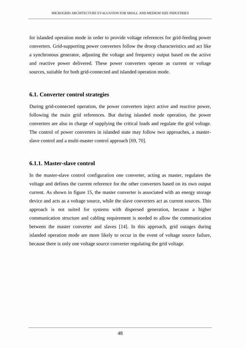
MICROGRID ARCHITECTURE EVALUATION FOR SMALL AND MEDIUM SIZE INDUSTRIES
48
for islanded operation mode in order to provide voltage references for grid-feeding power
converters. Grid-supporting power converters follow the droop characteristics and act like
a synchronous generator, adjusting the voltage and frequency output based on the active
and reactive power delivered. These power converters operate as current or voltage
sources, suitable for both grid-connected and islanded operation mode.
6.1. Converter control strategies
During grid-connected operation, the power converters inject active and reactive power,
following the main grid references. But during islanded mode operation, the power
converters are also in charge of supplying the critical loads and regulate the grid voltage.
The control of power converters in islanded state may follow two approaches, a master-
slave control and a multi-master control approach [69, 70].
6.1.1. Master-slave control
In the master-slave control configuration one converter, acting as master, regulates the
voltage and defines the current reference for the other converters based on its own output
current. As shown in figure 15, the master converter is associated with an energy storage
device and acts as a voltage source, while the slave converters act as current sources. This
approach is not suited for systems with dispersed generation, because a higher
communication structure and cabling requirement is needed to allow the communication
between the master converter and slaves [14]. In this approach, grid outages during
islanded operation mode are more likely to occur in the event of voltage source failure,
because there is only one voltage source converter regulating the grid voltage.
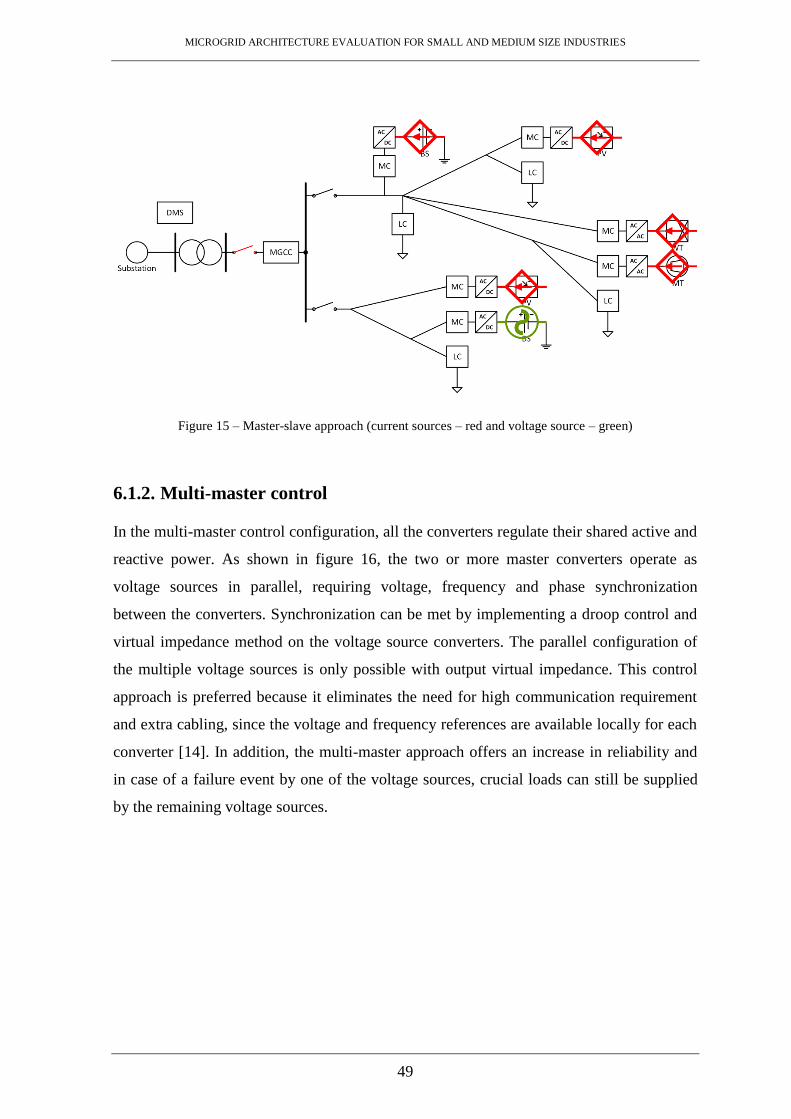
MICROGRID ARCHITECTURE EVALUATION FOR SMALL AND MEDIUM SIZE INDUSTRIES
49
Figure 15 – Master-slave approach (current sources – red and voltage source – green)
6.1.2. Multi-master control
In the multi-master control configuration, all the converters regulate their shared active and
reactive power. As shown in figure 16, the two or more master converters operate as
voltage sources in parallel, requiring voltage, frequency and phase synchronization
between the converters. Synchronization can be met by implementing a droop control and
virtual impedance method on the voltage source converters. The parallel configuration of
the multiple voltage sources is only possible with output virtual impedance. This control
approach is preferred because it eliminates the need for high communication requirement
and extra cabling, since the voltage and frequency references are available locally for each
converter [14]. In addition, the multi-master approach offers an increase in reliability and
in case of a failure event by one of the voltage sources, crucial loads can still be supplied
by the remaining voltage sources.

MICROGRID ARCHITECTURE EVALUATION FOR SMALL AND MEDIUM SIZE INDUSTRIES
50
Figure 16 – Multi-master approach (current sources – red and voltage sources – green)
MICROGRID ARCHITECTURE EVALUATION FOR SMALL AND MEDIUM SIZE INDUSTRIES
51
7. MICROGRID PROTECTION
The main requirements for protection systems rely on selectivity, sensitivity and speed.
Selectivity aims at disconnecting the minimum grid section possible in order to isolate the
fault and maintaining the supply of power to the loads. Sensitivity aims at detecting any
abnormal condition exceeding the nominal value. Speed refers to the minimum response
time to deal with a fault and avoid further damage to the system. It is also required the
maximum possible protection at the lowest cost and the system must be reliable and stable
during different operating conditions. In the absence of these protection requirements,
problems related to false tripping due to over sensitive protection devices, delayed tripping
due to protection devices with a slow response time and faults that remain undetected may
arise during certain operating conditions [14]. Due to the integration of DG units with
power converter interfaces and the high penetration of synchronous and asynchronous
generators, MGs bring several protection issues and challenges. The DG units dispersed
along the grid and connected at different locations may cause the power flow in the
distribution grid to change from uni-directional to bi-directional if the local power
generation exceeds the power demand. In addition, the fault current in a MG is
significantly lower during islanded operation mode, because the power converter interfaces
associated with the DG units limit the fault current and thus do not supply sufficient
current to trigger some of the protection devices. In grid-connected mode, the fault current
can be detected by the protection devices, since the public power grid provides an increase
in fault current. The high penetration of rotating machines such as synchronous and
asynchronous generators into the grid may cause the fault current level to exceed the
equipment ratings and cause damage [71]. Moreover, changing fault current levels can be a
result of the connection of several DG units with intermittent nature such as photovoltaic
(PV) generation systems during islanded operation mode.
The protection system of a MG must be able to quickly react to the public power grid
faults and respond to MG failures in order to prevent further damage. The MG transitions
between grid-connected and islanded state by means of a static switch that separates the
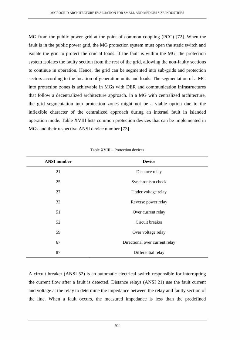
MICROGRID ARCHITECTURE EVALUATION FOR SMALL AND MEDIUM SIZE INDUSTRIES
52
MG from the public power grid at the point of common coupling (PCC) [72]. When the
fault is in the public power grid, the MG protection system must open the static switch and
isolate the grid to protect the crucial loads. If the fault is within the MG, the protection
system isolates the faulty section from the rest of the grid, allowing the non-faulty sections
to continue in operation. Hence, the grid can be segmented into sub-grids and protection
sectors according to the location of generation units and loads. The segmentation of a MG
into protection zones is achievable in MGs with DER and communication infrastructures
that follow a decentralized architecture approach. In a MG with centralized architecture,
the grid segmentation into protection zones might not be a viable option due to the
inflexible character of the centralized approach during an internal fault in islanded
operation mode. Table XVIII lists common protection devices that can be implemented in
MGs and their respective ANSI device number [73].
Table XVIII – Protection devices
ANSI number Device
21 Distance relay
25 Synchronism check
27 Under voltage relay
32 Reverse power relay
51 Over current relay
52 Circuit breaker
59 Over voltage relay
67 Directional over current relay
87 Differential relay
A circuit breaker (ANSI 52) is an automatic electrical switch responsible for interrupting
the current flow after a fault is detected. Distance relays (ANSI 21) use the fault current
and voltage at the relay to determine the impedance between the relay and faulty section of
the line. When a fault occurs, the measured impedance is less than the predefined

MICROGRID ARCHITECTURE EVALUATION FOR SMALL AND MEDIUM SIZE INDUSTRIES
53
impedance and the relay issues a trip signal to the circuit breaker. Overcurrent relays
(ANSI 51) operate when the current exceeds a predefined value and issue a trip signal to
the circuit breaker. Directional overcurrent relays (ANSI 67) uses the phase difference
between voltage and current to determine the direction to a fault. Reverse power relays
(ANSI 32) are directional relays often used in generators to prevent the power from
flowing in the reverse direction. When the output of the active generator drops below a
predefined value, the relay disconnects the generator to prevent the power from flowing
back into the generator. Synchronism check relays (ANSI 25) keep a circuit breaker closed
when the measured voltages on both sides are within predefined limits of magnitude, phase
angle and frequency. In case of any deviation in frequency between the two sides, the
circuit breaker is opened. Overvoltage relays (ANSI 59) operate when the measured
voltage exceeds a predefined limit and trigger the circuit breaker to open. Undervoltage
relays (ANSI 27) operate when the measured voltage drops below a predefined value.
Differential relays (ANSI 87) are used to protect distribution lines, generators and
transformers by determining the difference between two or more identical electrical
quantities. When a fault occurs, the difference between the input current and output current
is not zero and a trip signal is sent to the circuit breakers.
Figure 17 – Requirement for feeders, buses and generation units
Several protection methodologies for MGs are available in the literature. Jenkins et al. in
[74] proposed a protection plan using overcurrent relays for grid-connected operation
mode. Al-Nasseri et al. in [75] presented a voltage-based protection scheme for islanded
operation mode. Then, Dewadasa et al. in [76] proposed a protection scheme using a
distance relay that could operate in both grid-connected and islanded modes. Years later,
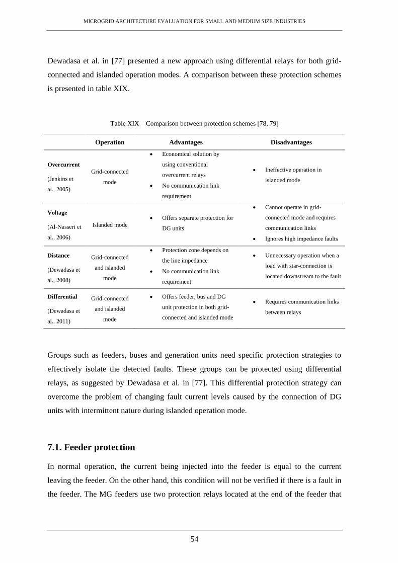
MICROGRID ARCHITECTURE EVALUATION FOR SMALL AND MEDIUM SIZE INDUSTRIES
54
Dewadasa et al. in [77] presented a new approach using differential relays for both grid-
connected and islanded operation modes. A comparison between these protection schemes
is presented in table XIX.
Table XIX – Comparison between protection schemes [78, 79]
Operation Advantages Disadvantages
Overcurrent
(Jenkins et
al., 2005)
Grid-connected
mode
Economical solution by
using conventional
overcurrent relays
No communication link
requirement
Ineffective operation in
islanded mode
Voltage
(Al-Nasseri et
al., 2006)
Islanded mode
Offers separate protection for
DG units
Cannot operate in grid-
connected mode and requires
communication links
Ignores high impedance faults
Distance
(Dewadasa et
al., 2008)
Grid-connected
and islanded
mode
Protection zone depends on
the line impedance
No communication link
requirement
Unnecessary operation when a
load with star-connection is
located downstream to the fault
Differential
(Dewadasa et
al., 2011)
Grid-connected
and islanded
mode
Offers feeder, bus and DG
unit protection in both grid-
connected and islanded mode
Requires communication links
between relays
Groups such as feeders, buses and generation units need specific protection strategies to
effectively isolate the detected faults. These groups can be protected using differential
relays, as suggested by Dewadasa et al. in [77]. This differential protection strategy can
overcome the problem of changing fault current levels caused by the connection of DG
units with intermittent nature during islanded operation mode.
7.1. Feeder protection
In normal operation, the current being injected into the feeder is equal to the current
leaving the feeder. On the other hand, this condition will not be verified if there is a fault in
the feeder. The MG feeders use two protection relays located at the end of the feeder that

MICROGRID ARCHITECTURE EVALUATION FOR SMALL AND MEDIUM SIZE INDUSTRIES
55
detect and isolate feeder faults. Differential relays (ANSI 87) are not sensible to bi-
directional power flow and change in the number of connections, making these relays
preferred for MG feeder protection. The relays contain five elements including three phase
elements for each phase to provide high speed protection against high current faults, and
two elements for the negative and zero sequence currents to ensure a sensitive protection
against lower currents faults. As shown in figure 18, each relay issues a trip signal to the
respective local circuit breaker when a fault is detected. The relays at each end of the
feeder are connected through a communication link and share synchronized phase current
samples [77].
Figure 18 – Differential feeder protection
In a decentralized architecture where the DG units are dispersed along the grid and
connected at different locations, the use of a circuit breaker at each end of a feeder can be
justified due to bi-directional power flow. However, in case of a centralized architecture
where the power flows from the generation group to loads, using a circuit breaker at each
end of a feeder increases the cost and might not be economically viable, especially in
applications for SMEs. A single circuit breaker feeder configuration can be implemented in
branches with uni-directional power flow in order to reduce the cost in both centralized and
decentralized grid architectures. The circuit breaker should be deployed at the beginning of
the feeder, defined as the side in which the current enters.
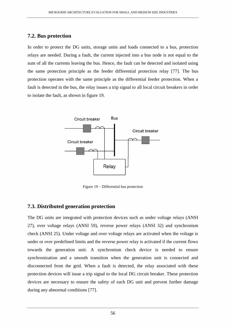
MICROGRID ARCHITECTURE EVALUATION FOR SMALL AND MEDIUM SIZE INDUSTRIES
56
7.2. Bus protection
In order to protect the DG units, storage units and loads connected to a bus, protection
relays are needed. During a fault, the current injected into a bus node is not equal to the
sum of all the currents leaving the bus. Hence, the fault can be detected and isolated using
the same protection principle as the feeder differential protection relay [77]. The bus
protection operates with the same principle as the differential feeder protection. When a
fault is detected in the bus, the relay issues a trip signal to all local circuit breakers in order
to isolate the fault, as shown in figure 19.
Figure 19 – Differential bus protection
7.3. Distributed generation protection
The DG units are integrated with protection devices such as under voltage relays (ANSI
27), over voltage relays (ANSI 59), reverse power relays (ANSI 32) and synchronism
check (ANSI 25). Under voltage and over voltage relays are activated when the voltage is
under or over predefined limits and the reverse power relay is activated if the current flows
towards the generation unit. A synchronism check device is needed to ensure
synchronization and a smooth transition when the generation unit is connected and
disconnected from the grid. When a fault is detected, the relay associated with these
protection devices will issue a trip signal to the local DG circuit breaker. These protection
devices are necessary to ensure the safety of each DG unit and prevent further damage
during any abnormal conditions [77].

MICROGRID ARCHITECTURE EVALUATION FOR SMALL AND MEDIUM SIZE INDUSTRIES
57
7.4. Earthing system
The earthing system of LV distribution networks can be categorized in three
configurations, TT, IT and TN [80]. These three configurations are defined by five letters,
T (direct connection to earth), N (neutral), C (combined), S (separated) and I (isolated from
earth). The first letter indicates how the transformer neutral or supply source is earthed and
the second letter indicates how the equipment frame is earthed. The third or fourth letters
indicate the configuration of the neutral and protective earth conductors and denote their
functions [81].
In a TT system, both the transformer neutral and the equipment frames are earthed directly
by an earth electrode, as represented in figure 20. It is the most simple and common
earthing system, often used in networks containing distributed equipment such as public
lighting networks.
Figure 20 – TT earthing system protection
In an IT system, the transformer neutral is not earthed or not earthed directly and the
equipment frames are earthed directly, as represented in figure 21. It is usually used for
systems that require high security and reliability.

MICROGRID ARCHITECTURE EVALUATION FOR SMALL AND MEDIUM SIZE INDUSTRIES
58
Figure 21 – IT earthing system protection
In a TN system, the transformer neutral is earthed directly and the equipment frames are
connected to neutral conductors. TN earthing systems are subdivided in TN-C, TN-S and
TN-C-S. TN-C systems combine the neutral conductor (N) and the protective earth
conductor (PE) in a single conductor (Protective Earth Neutral, PEN), the same conductor
is used for both neutral and protective functions, as represented in figure 22. TN-S systems
use different conductors for the neutral and protective functions. As represented in figure
23, the neutral conductor (N) is separated from the protective earth conductor (PE). The
TN-C-S system combines both the TN-C and TN-S earthing systems. This system uses a
common PEN conductor at the power supply and is then separated in neutral conductor (N)
and protective earth conductor (PE) near the loads, as represented in figure 24.
Figure 22 – TN-C earthing system protection
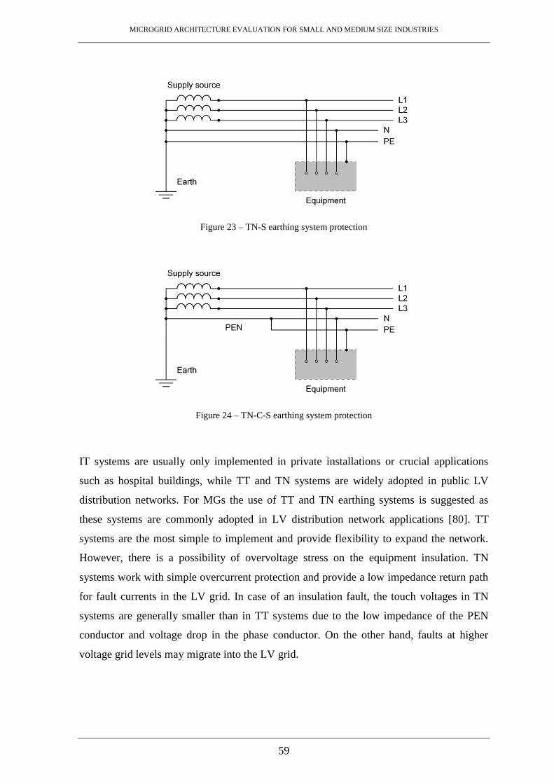
MICROGRID ARCHITECTURE EVALUATION FOR SMALL AND MEDIUM SIZE INDUSTRIES
59
Figure 23 – TN-S earthing system protection
Figure 24 – TN-C-S earthing system protection
IT systems are usually only implemented in private installations or crucial applications
such as hospital buildings, while TT and TN systems are widely adopted in public LV
distribution networks. For MGs the use of TT and TN earthing systems is suggested as
these systems are commonly adopted in LV distribution network applications [80]. TT
systems are the most simple to implement and provide flexibility to expand the network.
However, there is a possibility of overvoltage stress on the equipment insulation. TN
systems work with simple overcurrent protection and provide a low impedance return path
for fault currents in the LV grid. In case of an insulation fault, the touch voltages in TN
systems are generally smaller than in TT systems due to the low impedance of the PEN
conductor and voltage drop in the phase conductor. On the other hand, faults at higher
voltage grid levels may migrate into the LV grid.

MICROGRID ARCHITECTURE EVALUATION FOR SMALL AND MEDIUM SIZE INDUSTRIES
60
According to the study presented in [81], the most suitable earthing system for MGs during
islanded operation mode is the TN-S. Since the fault current may not be detected in an
islanded MG with intermittent DG units, the TN-S system overcomes this problem because
the fault current in this system is sufficient enough to trigger the protection devices.
Furthermore, protection relays are capable of discriminating between overload current and
fault current in a MG with TN-S earthing system implemented.

MICROGRID ARCHITECTURE EVALUATION FOR SMALL AND MEDIUM SIZE INDUSTRIES
61
8. CASE STUDY
This section presents a case study of an industrial MG with centralized and decentralized
architecture. The industrial MG developed for this study is based on the transformer, cable,
generator and load data presented in [82, 83]. The purpose of this section is to observe how
a centralized and decentralized deployment of DERs affects the performance of a small
scale industrial MG. The industrial site under study is a small factory that produces paper
sheets. It contains a main factory and offices with a nominal power consumption of 320
kW and 80 kW, respectively. There are four step-down transformers inside the MG,
transformers T1 and T2 are responsible for decreasing the voltage from 13.8 kV to 480 V,
and T3 and T4 decrease the voltage from 480 V to 208 V in order to supply loads such as
lights and office equipment. The factory building contains five induction motors, two air
conditioning units, an elevator and lights. The office building contains an air conditioning
unit, lights and office equipment such as personal computers, printers and fax machines.
Figure 25 represents the electrical schematic of the small industrial site under study. The
data for each load and transformer is listed in table XX and XXI.
Table XX – Load data
Load Quantity Voltage (V) Unit size (kW) Power factor R (Ω) X (Ω)
Induction motor 5 480 50 0.8 2.946 2.21
Office equipment 4 208 12.5 0.96 1.065 0.307
Air conditioning 3 480 15 0.95 13.844 4.517
Elevator 1 480 30 0.97 7.234 1.804
Light (factory) 5 208 2 0.98 6.92 1.38
Light (offices) 5 208 3 0.98 4.60 0.917

MICROGRID ARCHITECTURE EVALUATION FOR SMALL AND MEDIUM SIZE INDUSTRIES
62
Table XXI – Transformer data
Transformer Primary (kV) Secondary (kV) Load (kW) Rating (kVA) R (Ω) X (Ω)
T1 13.8 0.480 80 200 7.2 29.52
T2 13.8 0.480 320 1000 1.15 8.95
T3 0.480 0.208 65 200 0.0087 0.0357
T4 0.480 0.208 10 40 0.038 0.1440
Figure 25 – Electrical schematic of the industrial site
During islanded mode operation, the power generator that simulates the public grid is
disconnected from the MG at the PCC. All the loads in the MG follow a priority according
to how important they are to the industrial process. Crucial loads are set to high priority
and must be supplied in all circumstances in order to avoid jeopardizing the production
targets. These loads include the five induction motors with a total power demand of 250

MICROGRID ARCHITECTURE EVALUATION FOR SMALL AND MEDIUM SIZE INDUSTRIES
63
kW located in the factory. The office equipment with a total power demand of 50 kW is set
to a medium priority. These loads should be supplied during islanded mode, but they can
also be disconnected if the available energy is insufficient to supply them. The remaining
loads such as lights, air conditioning units and elevator are set to a low priority. These
loads are disconnected from the grid during islanded mode. Both centralized and
decentralized MGs will be subjected to the same case scenarios in order to compare their
bus voltage and angle profiles obtained from the power flow study using the software
PSS/E Xplore.
This initial case is the base scenario and it is equivalent to both centralized and
decentralized MG configurations, since all the buses with generation units are disconnected
from the MG. In this scenario, the industrial MG is connected to the public grid and both
factory and offices are operating at full load (400 kW). All the loads are supplied by the
public grid without any power supply from the MG generation units. The public grid must
deliver 400 kW in order to supply the loads in the main factory (320 kW) and offices (80
kW). Tables XXII and XXIII show the results obtained from the power flow study for this
scenario.
Table XXII – Network generator data
Generator Bus PGen (MW) QGen (MVAr)
Public grid 1 0.4002 0.8855
Table XXIII – Network bus data
Bus Bus name Base voltage (kV) Voltage (pu) Angle (deg)
1 SWING 13.8 1.0000 0
2 BUS2 0.480 0.9996 -0.0046
3 BUS3 0.480 0.9997 -0.0057
4 BUS4 0.480 0.9996 -0.0013
5 BUS5 0.480 0.9996 -0.0049
6 LOAD1 0.480 0.9996 0.0014

MICROGRID ARCHITECTURE EVALUATION FOR SMALL AND MEDIUM SIZE INDUSTRIES
64
7 LOAD2 0.208 0.9992 -0.0018
8 LOAD3 0.208 0.9992 -0.0038
9 LOAD4 0.480 0.9994 0.0147
10 LOAD5 0.480 0.9995 -0.0045
The voltage obtained for each bus is almost ideal, approximately 1 pu for all buses with the
lowest voltage being 0.9992 pu in bus 7 (LOAD2) and bus 8 (LOAD3). This is due to the
small grid size and the public grid setting the bus voltage to 1 pu. The results listed in table
XXIII show the bus voltage and angle profile for a scenario without power generation from
any MG generation units. This initial scenario is compared with the five scenarios for each
MG configuration, in the next sections 8.1 and 8.2.
8.1. Centralized MG
A centralized MG architecture for this industrial site is represented in figure 26 and
includes a centralized generation group with 360 kW of peak power located at the
generation bus, GEN1. This generation group acts as an uninterruptible power generator
equipped with a bank of batteries and supplies the crucial loads in the main factory and the
office equipment when the available energy is sufficient. The branch data for this
configuration is listed in table XXIV.
Table XXIV – Branch data
Branch Voltage (kV) Load (kW) Distance (m) R (Ω) X (Ω)
4 ↔ 2 0.480 360 30 0.002 0.0027
4 ↔ 3 0.480 360 30 0.002 0.0027
2 ↔ 5 0.480 80 30 0.0052 0.0026
5 ↔ 7 0.480 15 10 0.024 0.0015
3 ↔ 6 0.480 320 30 0.002 0.0027
6 ↔ 10 0.480 60 40 0.0392 0.0064

MICROGRID ARCHITECTURE EVALUATION FOR SMALL AND MEDIUM SIZE INDUSTRIES
65
6 ↔ 11 0.480 250 30 0.0023 0.0025
Figure 26 – Schematic of the MG with centralized generation
8.1.1. Case 1C
In this scenario, the MG is connected to the public grid and both factory and offices are
operating at full load (400 kW). The loads are supplied by the generation group (GEN1) at
peak power generation capacity (360 kW) and the public grid delivers the power needed to
supply the remaining loads (40 kW). This represents the most satisfactory scenario during
grid-connected operation mode, since the generation group is at its peak power and
minimum power is imported from the public grid. Tables XXV and XXVI show the results
obtained from the power flow study for this scenario, and the bus voltage and angle
profiles are shown in figures 27 and 28.
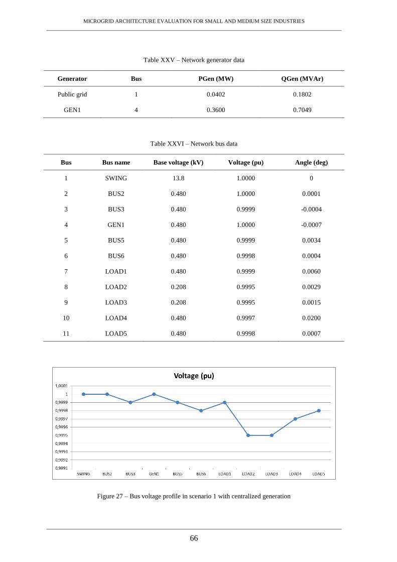
MICROGRID ARCHITECTURE EVALUATION FOR SMALL AND MEDIUM SIZE INDUSTRIES
66
Table XXV – Network generator data
Generator Bus PGen (MW) QGen (MVAr)
Public grid 1 0.0402 0.1802
GEN1 4 0.3600 0.7049
Table XXVI – Network bus data
Bus Bus name Base voltage (kV) Voltage (pu) Angle (deg)
1 SWING 13.8 1.0000 0
2 BUS2 0.480 1.0000 0.0001
3 BUS3 0.480 0.9999 -0.0004
4 GEN1 0.480 1.0000 -0.0007
5 BUS5 0.480 0.9999 0.0034
6 BUS6 0.480 0.9998 0.0004
7 LOAD1 0.480 0.9999 0.0060
8 LOAD2 0.208 0.9995 0.0029
9 LOAD3 0.208 0.9995 0.0015
10 LOAD4 0.480 0.9997 0.0200
11 LOAD5 0.480 0.9998 0.0007
Figure 27 – Bus voltage profile in scenario 1 with centralized generation
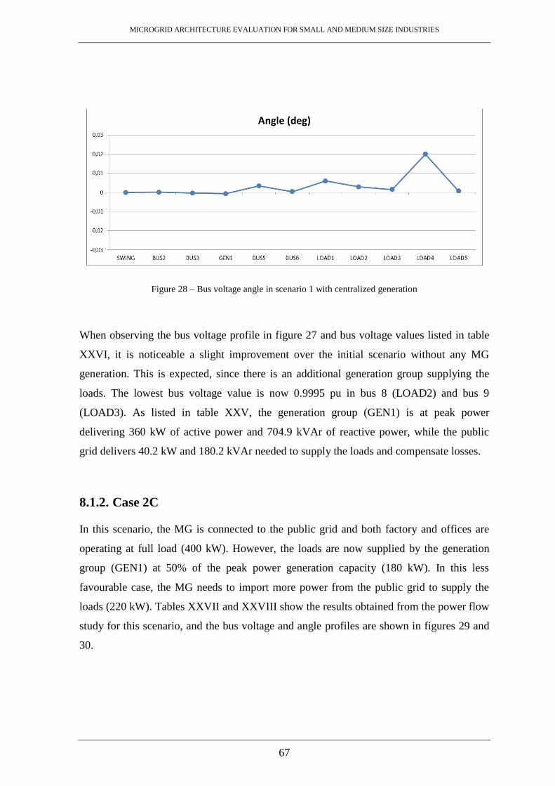
MICROGRID ARCHITECTURE EVALUATION FOR SMALL AND MEDIUM SIZE INDUSTRIES
67
Figure 28 – Bus voltage angle in scenario 1 with centralized generation
When observing the bus voltage profile in figure 27 and bus voltage values listed in table
XXVI, it is noticeable a slight improvement over the initial scenario without any MG
generation. This is expected, since there is an additional generation group supplying the
loads. The lowest bus voltage value is now 0.9995 pu in bus 8 (LOAD2) and bus 9
(LOAD3). As listed in table XXV, the generation group (GEN1) is at peak power
delivering 360 kW of active power and 704.9 kVAr of reactive power, while the public
grid delivers 40.2 kW and 180.2 kVAr needed to supply the loads and compensate losses.
8.1.2. Case 2C
In this scenario, the MG is connected to the public grid and both factory and offices are
operating at full load (400 kW). However, the loads are now supplied by the generation
group (GEN1) at 50% of the peak power generation capacity (180 kW). In this less
favourable case, the MG needs to import more power from the public grid to supply the
loads (220 kW). Tables XXVII and XXVIII show the results obtained from the power flow
study for this scenario, and the bus voltage and angle profiles are shown in figures 29 and
30.

MICROGRID ARCHITECTURE EVALUATION FOR SMALL AND MEDIUM SIZE INDUSTRIES
68
Table XXVII – Network generator data
Generator Bus PGen (MW) QGen (MVAr)
Public grid 1 0.2202 0.1339
GEN1 4 0.1800 0.7513
Table XXVIII – Network bus data
Bus Bus name Base voltage (kV) Voltage (pu) Angle (deg)
1 SWING 13.8 1.0000 0
2 BUS2 0.480 1.0000 -0.0043
3 BUS3 0.480 0.9999 -0.0041
4 GEN1 0.480 1.0000 -0.0055
5 BUS5 0.480 0.9999 -0.0010
6 BUS6 0.480 0.9998 -0.0033
7 LOAD1 0.480 0.9999 0.0016
8 LOAD2 0.208 0.9995 -0.0015
9 LOAD3 0.208 0.9995 -0.0023
10 LOAD4 0.480 0.9997 0.0163
11 LOAD5 0.480 0.9998 -0.0030
Figure 29 – Bus voltage profile in scenario 2 with centralized generation

MICROGRID ARCHITECTURE EVALUATION FOR SMALL AND MEDIUM SIZE INDUSTRIES
69
Figure 30 – Bus voltage angle in scenario 2 with centralized generation
When observing the bus voltage profile in figure 29 and bus voltage values listed in table
XXVIII, it is also noticeable an improvement over the initial scenario. This is expected,
since there is an additional generation group supplying the loads. The lowest bus voltage
value is also 0.9995 pu in bus 8 (LOAD2) and bus 9 (LOAD3). As listed in table XXVII,
the generation group (GEN1) is at 50% of the peak power generation capacity delivering
180 kW of active power and 751.3 kVAr of reactive power, while the public grid delivers
220.2 kW and 133.9 kVAr needed to supply the loads and compensate losses.
8.1.3. Case 3C
In this scenario, the MG is also connected to the public grid. But the main factory and
offices are now operating at 75% (240 kW) and 25% (20 kW), respectively. In the main
factory, both air conditioning units and an induction motor are out of service. In the office,
most of the lights and office equipment are not in use and the air conditioning unit is also
out of service. The loads are supplied by the generation group (GEN1) at 75% of the peak
power generation capacity (270 kW). Tables XXIX and XXX show the results obtained
from the power flow study for this scenario, and the bus voltage and angle profiles are
shown in figures 31 and 32.
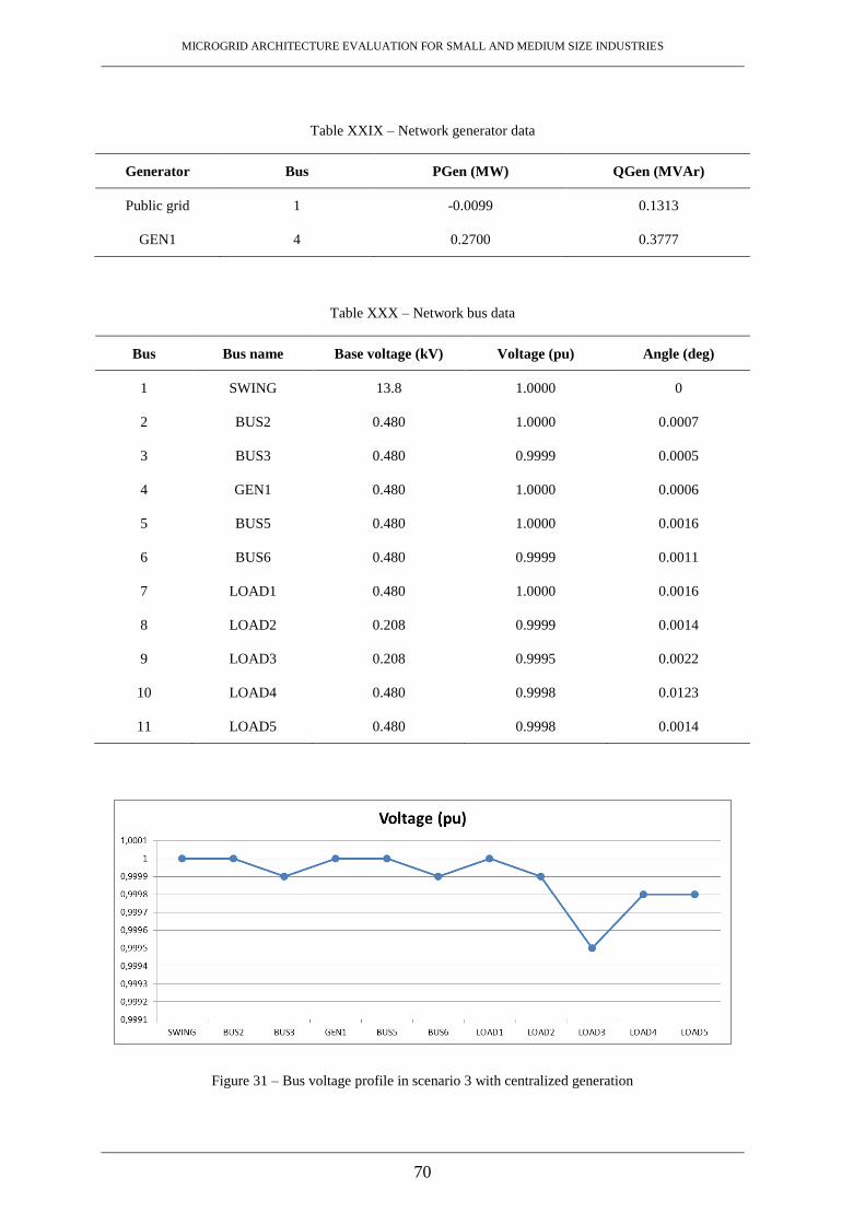
MICROGRID ARCHITECTURE EVALUATION FOR SMALL AND MEDIUM SIZE INDUSTRIES
70
Table XXIX – Network generator data
Generator Bus PGen (MW) QGen (MVAr)
Public grid 1 -0.0099 0.1313
GEN1 4 0.2700 0.3777
Table XXX – Network bus data
Bus Bus name Base voltage (kV) Voltage (pu) Angle (deg)
1 SWING 13.8 1.0000 0
2 BUS2 0.480 1.0000 0.0007
3 BUS3 0.480 0.9999 0.0005
4 GEN1 0.480 1.0000 0.0006
5 BUS5 0.480 1.0000 0.0016
6 BUS6 0.480 0.9999 0.0011
7 LOAD1 0.480 1.0000 0.0016
8 LOAD2 0.208 0.9999 0.0014
9 LOAD3 0.208 0.9995 0.0022
10 LOAD4 0.480 0.9998 0.0123
11 LOAD5 0.480 0.9998 0.0014
Figure 31 – Bus voltage profile in scenario 3 with centralized generation

MICROGRID ARCHITECTURE EVALUATION FOR SMALL AND MEDIUM SIZE INDUSTRIES
71
Figure 32 – Bus voltage angle in scenario 3 with centralized generation
When observing the bus voltage profile in figure 31 and bus voltage values listed in table
XXX, it is noticeable an improvement over the previous scenarios 1C and 2C, because
there was a decrease in power demand to 65% of the total power demand (260 kW). The
lowest bus voltage value is 0.9995 pu in bus 9 (LOAD3). As listed in table XXIX, the
generation group (GEN1) is at 75% of the peak power generation capacity delivering 270
kW of active power and 377.7 kVAr of reactive power. In this scenario, 9.9 kW of active
power is exported to the public grid.
8.1.4. Case 4C
In this scenario, there is no connection to the public grid. MG is operating in islanded
mode and all the high and medium priority loads are connected to the grid. The five
induction motors with a power demand of 250 kW and the office equipment with a power
demand of 50 kW are supplied by the generation group (GEN1) at peak power generation
capacity (360 kW). This is the most satisfactory scenario during islanded operation mode,
since the generation group is operating at its power peak and the higher priority loads can
remain in operation. Tables XXXI and XXXII show the results obtained from the power
flow study for this scenario, and the bus voltage and angle profiles are shown in figures 33
and 34.

MICROGRID ARCHITECTURE EVALUATION FOR SMALL AND MEDIUM SIZE INDUSTRIES
72
Table XXXI – Network generator data
Generator Bus PGen (MW) QGen (MVAr)
GEN1 4 0.3001 0.5052
Table XXXII – Network bus data
Bus Bus name Base voltage (kV) Voltage (pu) Angle (deg)
1 BUS1 13.8 0.9999 0.0001
2 BUS2 0.480 1.0000 0.0005
3 BUS3 0.480 0.9999 -0.00003
4 GEN1* 0.480 1.0000 0
5 BUS5 0.480 0.9999 0.0024
6 BUS6 0.480 0.9999 -0.00004
7 LOAD1 0.480 0.9999 0.0024
8 LOAD2 0.208 0.9997 0.0017
9 LOAD3 0.208 0.9999 -0.00004
10 LOAD4 0.480 0.9999 -0.00004
11 LOAD5 0.480 0.9998 0.0003
* Bus GEN1 is defined as slack bus (swing bus)
Figure 33 – Bus voltage profile in scenario 4 with centralized generation
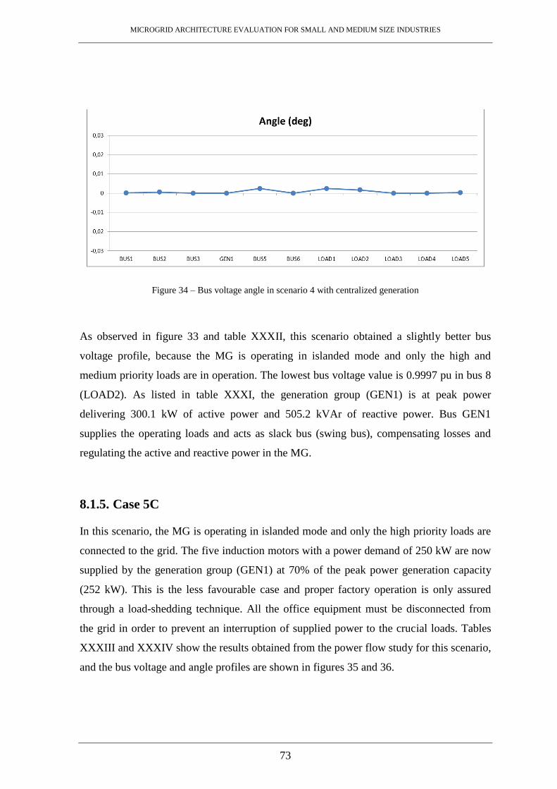
MICROGRID ARCHITECTURE EVALUATION FOR SMALL AND MEDIUM SIZE INDUSTRIES
73
Figure 34 – Bus voltage angle in scenario 4 with centralized generation
As observed in figure 33 and table XXXII, this scenario obtained a slightly better bus
voltage profile, because the MG is operating in islanded mode and only the high and
medium priority loads are in operation. The lowest bus voltage value is 0.9997 pu in bus 8
(LOAD2). As listed in table XXXI, the generation group (GEN1) is at peak power
delivering 300.1 kW of active power and 505.2 kVAr of reactive power. Bus GEN1
supplies the operating loads and acts as slack bus (swing bus), compensating losses and
regulating the active and reactive power in the MG.
8.1.5. Case 5C
In this scenario, the MG is operating in islanded mode and only the high priority loads are
connected to the grid. The five induction motors with a power demand of 250 kW are now
supplied by the generation group (GEN1) at 70% of the peak power generation capacity
(252 kW). This is the less favourable case and proper factory operation is only assured
through a load-shedding technique. All the office equipment must be disconnected from
the grid in order to prevent an interruption of supplied power to the crucial loads. Tables
XXXIII and XXXIV show the results obtained from the power flow study for this scenario,
and the bus voltage and angle profiles are shown in figures 35 and 36.

MICROGRID ARCHITECTURE EVALUATION FOR SMALL AND MEDIUM SIZE INDUSTRIES
74
Table XXXIII – Network generator data
Generator Bus PGen (MW) QGen (MVAr)
GEN1 4 0.2500 0.3336
Table XXXIV – Network bus data
Bus Bus name Base voltage (kV) Voltage (pu) Angle (deg)
1 BUS1 13.8 1.0000 0.00001
2 BUS2 0.480 1.0000 0.00008
3 BUS3 0.480 0.9999 -0.00009
4 GEN1* 0.480 1.0000 0
5 BUS5 0.480 1.0000 0.00008
6 BUS6 0.480 0.9999 -0.0001
7 LOAD1 0.480 1.0000 0.00008
8 LOAD2 0.208 1.0000 0.00008
9 LOAD3 0.208 0.9999 -0.0001
10 LOAD4 0.480 0.9999 -0.0001
11 LOAD5 0.480 0.9998 0.0002
* Bus GEN1 is defined as slack bus (swing bus)
Figure 35 – Bus voltage profile in scenario 5 with centralized generation

MICROGRID ARCHITECTURE EVALUATION FOR SMALL AND MEDIUM SIZE INDUSTRIES
75
Figure 36 – Bus voltage angle in scenario 5 with centralized generation
As observed in figure 35 and table XXXIV, there is a slight improvement in the bus
voltage profile obtained for this scenario when compared to the previous scenario 4C, since
the high priority loads are the only loads that remain in operation. The lowest bus voltage
value is now 0.9998 pu in bus 11 (LOAD5). As listed in table XXXIII, the generation
group (GEN1) is at 70% of the peak power generation capacity delivering 250 kW of
active power and 333.6 kVAr of reactive power. Bus GEN1 also needs to be defined as
slack bus (swing bus) and supplies the high priority loads.
8.2. Decentralized MG
A decentralized MG architecture for this industrial site is represented in figure 37 and
includes four generation groups located at the generation buses, GEN1, GEN2, GEN3 and
GEN4. The generation groups act as uninterruptible power generators equipped with a
bank of batteries dispersed along the grid and close to the higher priority loads. The branch
and generator group data for this configuration are listed in tables XXXV and XXXVI.

MICROGRID ARCHITECTURE EVALUATION FOR SMALL AND MEDIUM SIZE INDUSTRIES
76
Table XXXV – Cable data
Branch Voltage (kV) Load (kW) Distance (m) R (Ω) X (Ω)
4 ↔ 2 0.480 10 30 0.0052 0.0026
5 ↔ 3 0.480 50 30 0.002 0.0027
2 ↔ 6 0.480 80 30 0.0052 0.0026
6 ↔ 8 0.480 15 10 0.024 0.0015
3 ↔ 7 0.480 320 30 0.002 0.0027
7 ↔ 11 0.480 60 40 0.0392 0.0064
7 ↔ 12 0.480 250 30 0.0023 0.0025
13 ↔ 12 0.480 250 10 0.0023 0.0025
14 ↔ 9 0.208 50 10 0.024 0.0015
Table XXXVI – Generator group data
Bus Bus name Bus voltage (kV) Peak power (kW)
4 GEN1 0.480 10
5 GEN2 0.480 50
13 GEN3 0.480 250
14 GEN4 0.208 50

MICROGRID ARCHITECTURE EVALUATION FOR SMALL AND MEDIUM SIZE INDUSTRIES
77
Figure 37 – Schematic of the MG with decentralized generation
8.2.1. Case 1D
In this scenario, the MG is connected to the public grid and both factory and offices are
operating at full load (400 kW). The loads are supplied by the generation groups (GEN1,
GEN2, GEN3 and GEN4) at peak power generation capacity (360 kW) and the public grid
delivers the power needed to supply the remaining loads (40 kW). This represents the most
satisfactory scenario during grid-connected operation mode, since all the generation groups
are at their peak power and minimum power is imported from the public grid. Tables
XXXVII and XXXVIII show the results obtained from the power flow study for this
scenario, and the bus voltage and angle profiles are shown in figures 38 and 39.

MICROGRID ARCHITECTURE EVALUATION FOR SMALL AND MEDIUM SIZE INDUSTRIES
78
Table XXXVII – Network generator data
Generator Bus PGen (MW) QGen (MVAr)
Public grid 1 0.0402 0.0655
GEN1 4 0.0100 0.0675
GEN2 5 0.0500 0.1769
GEN3 13 0.2500 0.3529
GEN4 14 0.0500 0.2221
Table XXXVIII – Network bus data
Bus Bus name Base voltage (kV) Voltage (pu) Angle (deg)
1 SWING 13.8 1.0000 0
2 BUS2 0.480 1.0000 -0.0017
3 BUS3 0.480 1.0000 -0.0003
4 GEN1 0.480 1.0000 -0.0026
5 GEN2 0.480 1.0000 -0.0023
6 BUS6 0.480 1.0000 -0.0010
7 BUS7 0.480 0.9999 0.0004
8 LOAD1 0.480 1.0000 0.0016
9 LOAD2 0.208 0.9999 -0.0019
10 LOAD3 0.208 0.9996 0.0015
11 LOAD4 0.480 0.9998 0.0200
12 LOAD5 0.480 0.9999 0.0003
13 GEN3 0.480 1.0000 -0.0002
14 GEN4 0.208 1.0000 -0.0150

MICROGRID ARCHITECTURE EVALUATION FOR SMALL AND MEDIUM SIZE INDUSTRIES
79
Figure 38 – Bus voltage profile in scenario 1 with decentralized generation
Figure 39 – Bus voltage angle in scenario 1 with decentralized generation
The bus voltage profile in figure 38 and values listed in table XXXVIII show
improvements over the initial scenario. As observed, this scenario with decentralized
generation obtained a relatively better bus voltage profile than scenario 1C with centralized
generation. This is expected, since there are four generation groups dispersed along the
grid to supply the loads. The lowest bus voltage value is now 0.9996 pu in bus 10
(LOAD3). As listed in table XXXVII, the generation groups (GEN1, GEN2, GEN3 and
GEN4) are at their peak power delivering 360 kW of active power and 819.4 kVAr of
reactive power, while the public grid delivers 40.2 kW and 65.5 kVAr needed to supply the
loads and compensate losses.

MICROGRID ARCHITECTURE EVALUATION FOR SMALL AND MEDIUM SIZE INDUSTRIES
80
8.2.2. Case 2D
In this scenario, the MG is connected to the public grid and both factory and offices are
operating at full load (400 kW). However, the loads are now supplied by the generation
groups (GEN1, GEN2, GEN3 and GEN4) at 50% of the peak power generation capacity
(180 kW). In this less favourable case, the MG needs to import more power from the
public grid to supply the loads (220 kW). Tables XXXIX and XL show the results obtained
from the power flow study for this scenario, and the bus voltage and angle profiles are
shown in figures 40 and 41.
Table XXXIX – Network generator data
Generator Bus PGen (MW) QGen (MVAr)
Public grid 1 0.2202 0.0163
GEN1 4 0.0050 0.0543
GEN2 5 0.0250 0.1395
GEN3 13 0.1250 0.4305
GEN4 14 0.0250 0.2445
Table XL – Network bus data
Bus Bus name Base voltage (kV) Voltage (pu) Angle (deg)
1 SWING 13.8 1.0000 0
2 BUS2 0.480 1.0000 -0.0046
3 BUS3 0.480 1.0000 -0.0045
4 GEN1 0.480 1.0000 -0.0053
5 GEN2 0.480 1.0000 -0.0061
6 BUS6 0.480 1.0000 -0.0044
7 BUS7 0.480 0.9999 -0.0050
8 LOAD1 0.480 1.0000 -0.0017
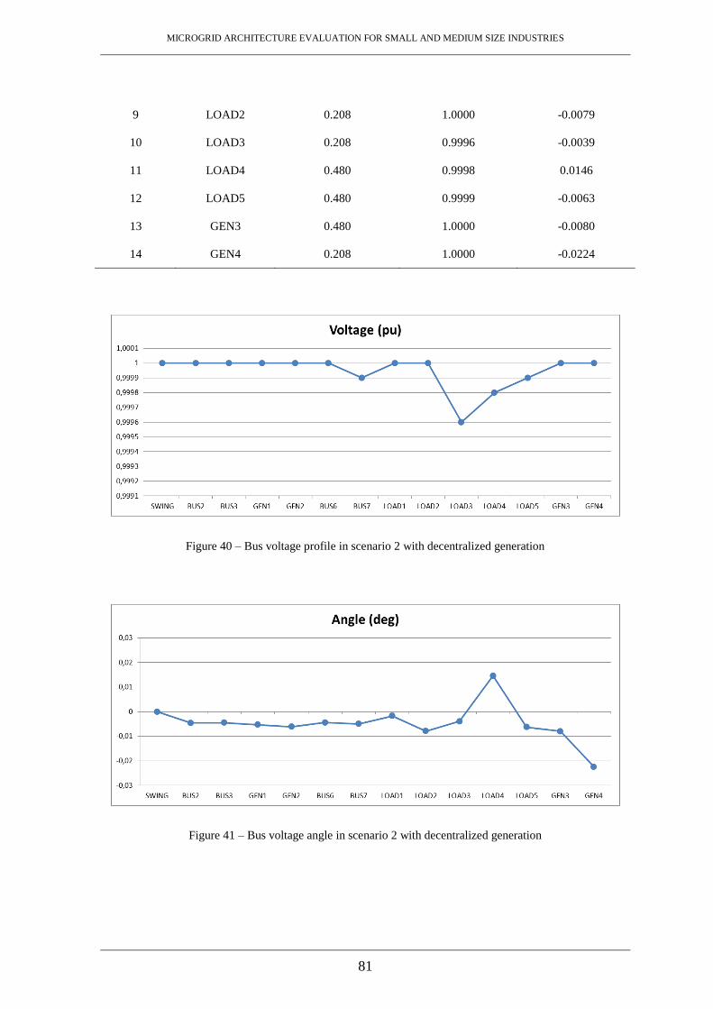
MICROGRID ARCHITECTURE EVALUATION FOR SMALL AND MEDIUM SIZE INDUSTRIES
81
9 LOAD2 0.208 1.0000 -0.0079
10 LOAD3 0.208 0.9996 -0.0039
11 LOAD4 0.480 0.9998 0.0146
12 LOAD5 0.480 0.9999 -0.0063
13 GEN3 0.480 1.0000 -0.0080
14 GEN4 0.208 1.0000 -0.0224
Figure 40 – Bus voltage profile in scenario 2 with decentralized generation
Figure 41 – Bus voltage angle in scenario 2 with decentralized generation
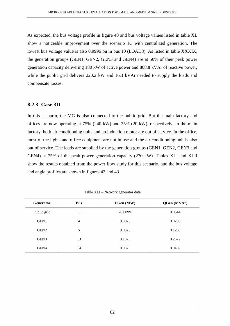
MICROGRID ARCHITECTURE EVALUATION FOR SMALL AND MEDIUM SIZE INDUSTRIES
82
As expected, the bus voltage profile in figure 40 and bus voltage values listed in table XL
show a noticeable improvement over the scenario 1C with centralized generation. The
lowest bus voltage value is also 0.9996 pu in bus 10 (LOAD3). As listed in table XXXIX,
the generation groups (GEN1, GEN2, GEN3 and GEN4) are at 50% of their peak power
generation capacity delivering 180 kW of active power and 868.8 kVAr of reactive power,
while the public grid delivers 220.2 kW and 16.3 kVAr needed to supply the loads and
compensate losses.
8.2.3. Case 3D
In this scenario, the MG is also connected to the public grid. But the main factory and
offices are now operating at 75% (240 kW) and 25% (20 kW), respectively. In the main
factory, both air conditioning units and an induction motor are out of service. In the office,
most of the lights and office equipment are not in use and the air conditioning unit is also
out of service. The loads are supplied by the generation groups (GEN1, GEN2, GEN3 and
GEN4) at 75% of the peak power generation capacity (270 kW). Tables XLI and XLII
show the results obtained from the power flow study for this scenario, and the bus voltage
and angle profiles are shown in figures 42 and 43.
Table XLI – Network generator data
Generator Bus PGen (MW) QGen (MVAr)
Public grid 1 -0.0099 0.0544
GEN1 4 0.0075 0.0205
GEN2 5 0.0375 0.1230
GEN3 13 0.1875 0.2672
GEN4 14 0.0375 0.0439
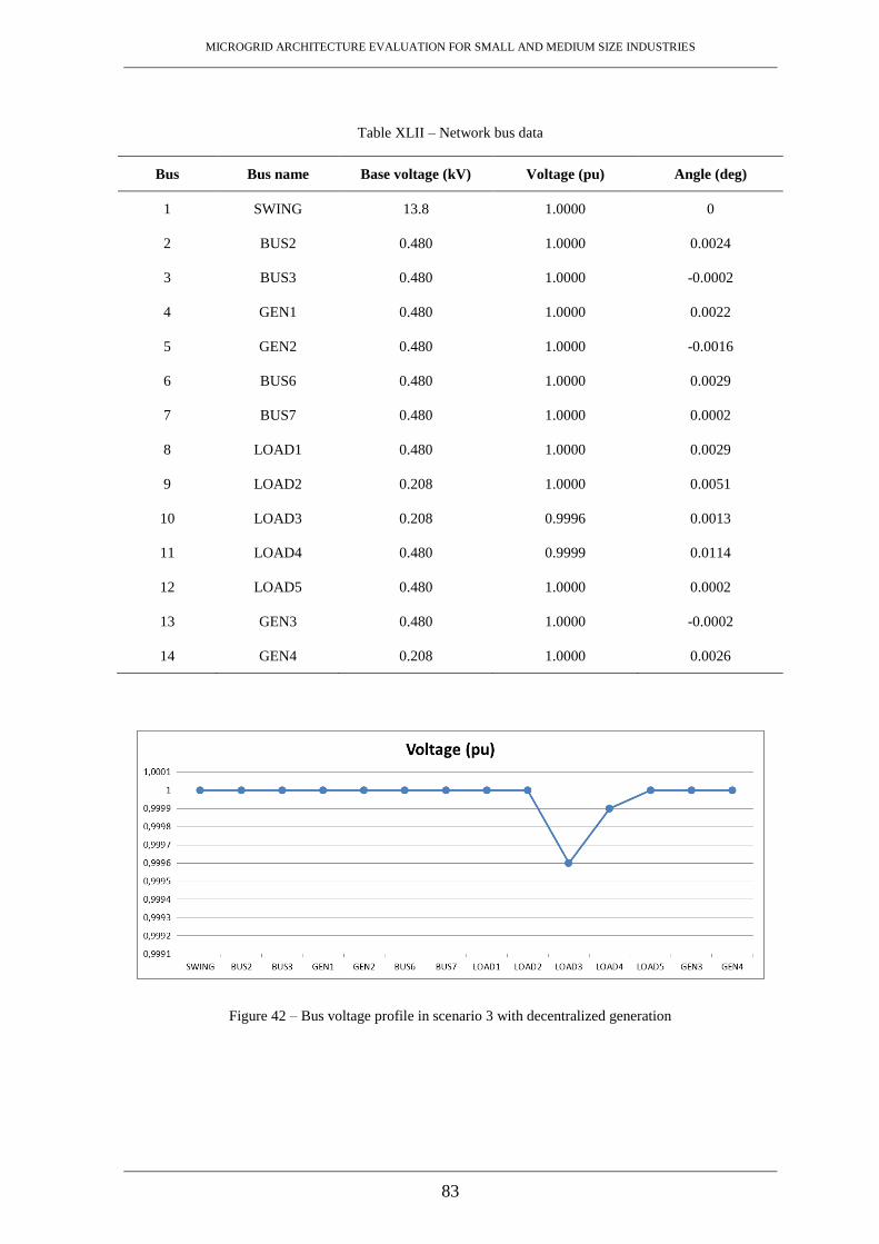
MICROGRID ARCHITECTURE EVALUATION FOR SMALL AND MEDIUM SIZE INDUSTRIES
83
Table XLII – Network bus data
Bus Bus name Base voltage (kV) Voltage (pu) Angle (deg)
1 SWING 13.8 1.0000 0
2 BUS2 0.480 1.0000 0.0024
3 BUS3 0.480 1.0000 -0.0002
4 GEN1 0.480 1.0000 0.0022
5 GEN2 0.480 1.0000 -0.0016
6 BUS6 0.480 1.0000 0.0029
7 BUS7 0.480 1.0000 0.0002
8 LOAD1 0.480 1.0000 0.0029
9 LOAD2 0.208 1.0000 0.0051
10 LOAD3 0.208 0.9996 0.0013
11 LOAD4 0.480 0.9999 0.0114
12 LOAD5 0.480 1.0000 0.0002
13 GEN3 0.480 1.0000 -0.0002
14 GEN4 0.208 1.0000 0.0026
Figure 42 – Bus voltage profile in scenario 3 with decentralized generation
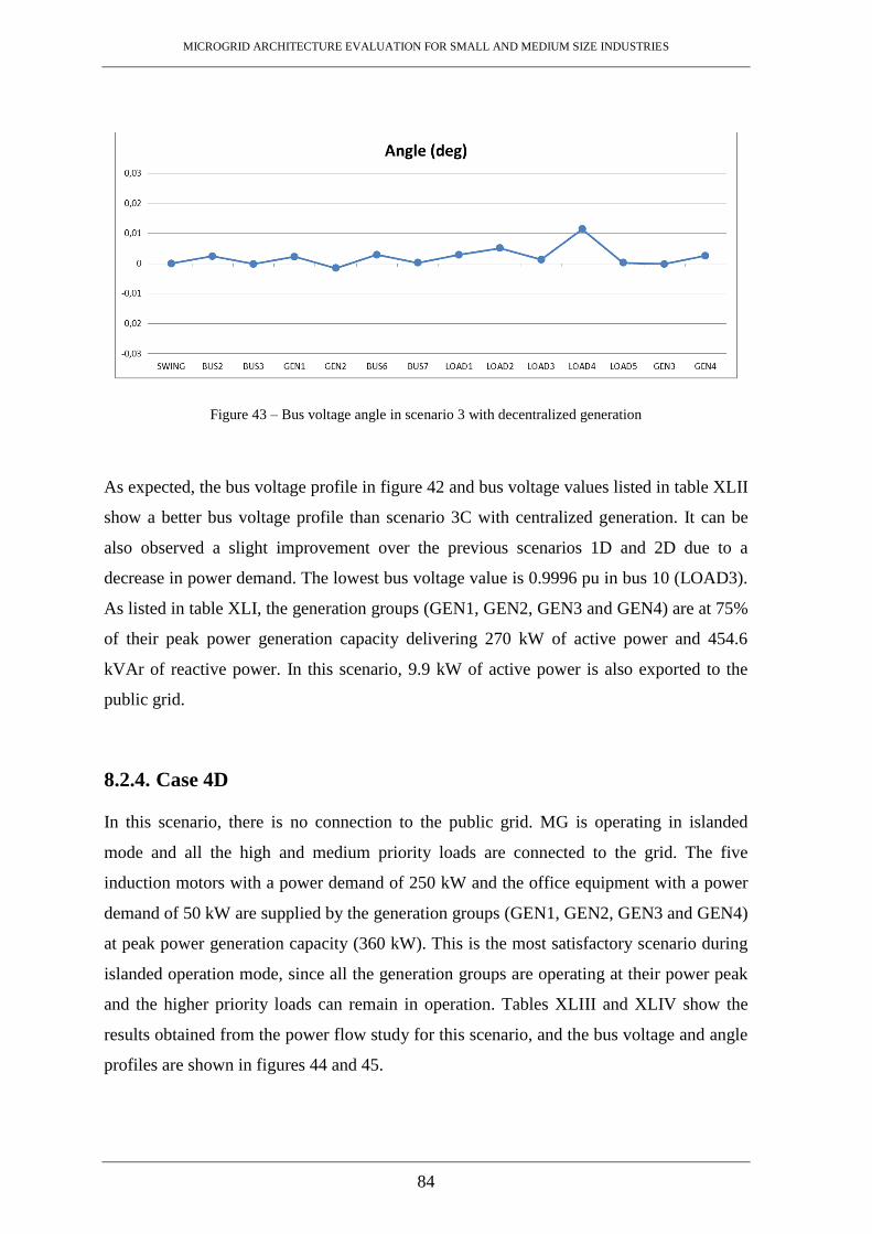
MICROGRID ARCHITECTURE EVALUATION FOR SMALL AND MEDIUM SIZE INDUSTRIES
84
Figure 43 – Bus voltage angle in scenario 3 with decentralized generation
As expected, the bus voltage profile in figure 42 and bus voltage values listed in table XLII
show a better bus voltage profile than scenario 3C with centralized generation. It can be
also observed a slight improvement over the previous scenarios 1D and 2D due to a
decrease in power demand. The lowest bus voltage value is 0.9996 pu in bus 10 (LOAD3).
As listed in table XLI, the generation groups (GEN1, GEN2, GEN3 and GEN4) are at 75%
of their peak power generation capacity delivering 270 kW of active power and 454.6
kVAr of reactive power. In this scenario, 9.9 kW of active power is also exported to the
public grid.
8.2.4. Case 4D
In this scenario, there is no connection to the public grid. MG is operating in islanded
mode and all the high and medium priority loads are connected to the grid. The five
induction motors with a power demand of 250 kW and the office equipment with a power
demand of 50 kW are supplied by the generation groups (GEN1, GEN2, GEN3 and GEN4)
at peak power generation capacity (360 kW). This is the most satisfactory scenario during
islanded operation mode, since all the generation groups are operating at their power peak
and the higher priority loads can remain in operation. Tables XLIII and XLIV show the
results obtained from the power flow study for this scenario, and the bus voltage and angle
profiles are shown in figures 44 and 45.

MICROGRID ARCHITECTURE EVALUATION FOR SMALL AND MEDIUM SIZE INDUSTRIES
85
Table XLIII – Network generator data
Generator Bus PGen (MW) QGen (MVAr)
GEN1 4 0.0100 0.0370
GEN2 5 0.0500 0.0702
GEN3 13 0.1900 0.2592
GEN4 14 0.0500 0.1387
Table XLIV – Network bus data
Bus Bus name Base voltage (kV) Voltage (pu) Angle (deg)
1 BUS1 13.8 1.0000 0.0005
2 BUS2 0.480 1.0000 0.0013
3 BUS3 0.480 1.0000 0.0003
4 GEN1 0.480 1.0000 0.0009
5 GEN2 0.480 1.0000 -0.0003
6 BUS6 0.480 1.0000 0.0018
7 BUS7 0.480 1.0000 0.0002
8 LOAD1 0.480 1.0000 0.0018
9 LOAD2 0.208 0.9999 0.0025
10 LOAD3 0.208 1.0000 0.0025
11 LOAD4 0.480 1.0000 0.0025
12 LOAD5 0.480 1.0000 0.0003
13 GEN3* 0.480 1.0000 0
14 GEN4 0.208 1.0000 -0.0056
* Bus GEN3 is defined as slack bus (swing bus)
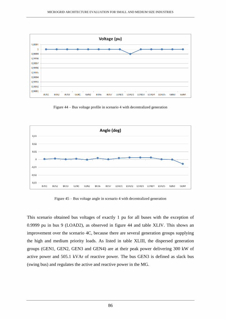
MICROGRID ARCHITECTURE EVALUATION FOR SMALL AND MEDIUM SIZE INDUSTRIES
86
Figure 44 – Bus voltage profile in scenario 4 with decentralized generation
Figure 45 – Bus voltage angle in scenario 4 with decentralized generation
This scenario obtained bus voltages of exactly 1 pu for all buses with the exception of
0.9999 pu in bus 9 (LOAD2), as observed in figure 44 and table XLIV. This shows an
improvement over the scenario 4C, because there are several generation groups supplying
the high and medium priority loads. As listed in table XLIII, the dispersed generation
groups (GEN1, GEN2, GEN3 and GEN4) are at their peak power delivering 300 kW of
active power and 505.1 kVAr of reactive power. The bus GEN3 is defined as slack bus
(swing bus) and regulates the active and reactive power in the MG.

MICROGRID ARCHITECTURE EVALUATION FOR SMALL AND MEDIUM SIZE INDUSTRIES
87
8.2.5. Case 5D
In this scenario, the MG is operating in islanded mode and only the high priority loads are
connected to the grid. The five induction motors with a power demand of 250 kW are now
supplied by the generation groups (GEN1, GEN2, GEN3 and GEN4) at 70% of the peak
power generation capacity (252 kW). This is the less favourable case and proper factory
operation is only assured through a load-shedding technique. All the office equipment must
be disconnected from the grid in order to prevent an interruption of supplied power to the
crucial loads. Tables XLV and XLVI show the results obtained from the power flow study
for this scenario, and the bus voltage and angle profiles are shown in figures 46 and 47.
Table XLV – Network generator data
Generator Bus PGen (MW) QGen (MVAr)
GEN1 4 0.0070 0.0272
GEN2 5 0.0350 0.0725
GEN3 13 0.1730 0.2644
GEN4 14 0.0350 -0.0307
Table XLVI – Network bus data
Bus Bus name Base voltage (kV) Voltage (pu) Angle (deg)
1 BUS1 13.8 1.0000 0.0018
2 BUS2 0.480 1.0000 0.0056
3 BUS3 0.480 1.0000 0.0007
4 GEN1 0.480 1.0000 0.0053
5 GEN2 0.480 1.0000 -0.00002
6 BUS6 0.480 1.0000 0.0063
7 BUS7 0.480 1.0000 0.0005
8 LOAD1 0.480 1.0000 0.0063
9 LOAD2 0.208 1.0000 0.0100

MICROGRID ARCHITECTURE EVALUATION FOR SMALL AND MEDIUM SIZE INDUSTRIES
88
10 LOAD3 0.208 1.0000 0.0005
11 LOAD4 0.480 1.0000 0.0005
12 LOAD5 0.480 1.0000 0.0004
13 GEN3* 0.480 1.0000 0
14 GEN4 0.208 1.0000 0.0120
* Bus GEN3 is defined as slack bus (swing bus)
Figure 46 – Bus voltage profile in scenario 5 with decentralized generation
Figure 47 – Bus voltage angle in scenario 5 with decentralized generation
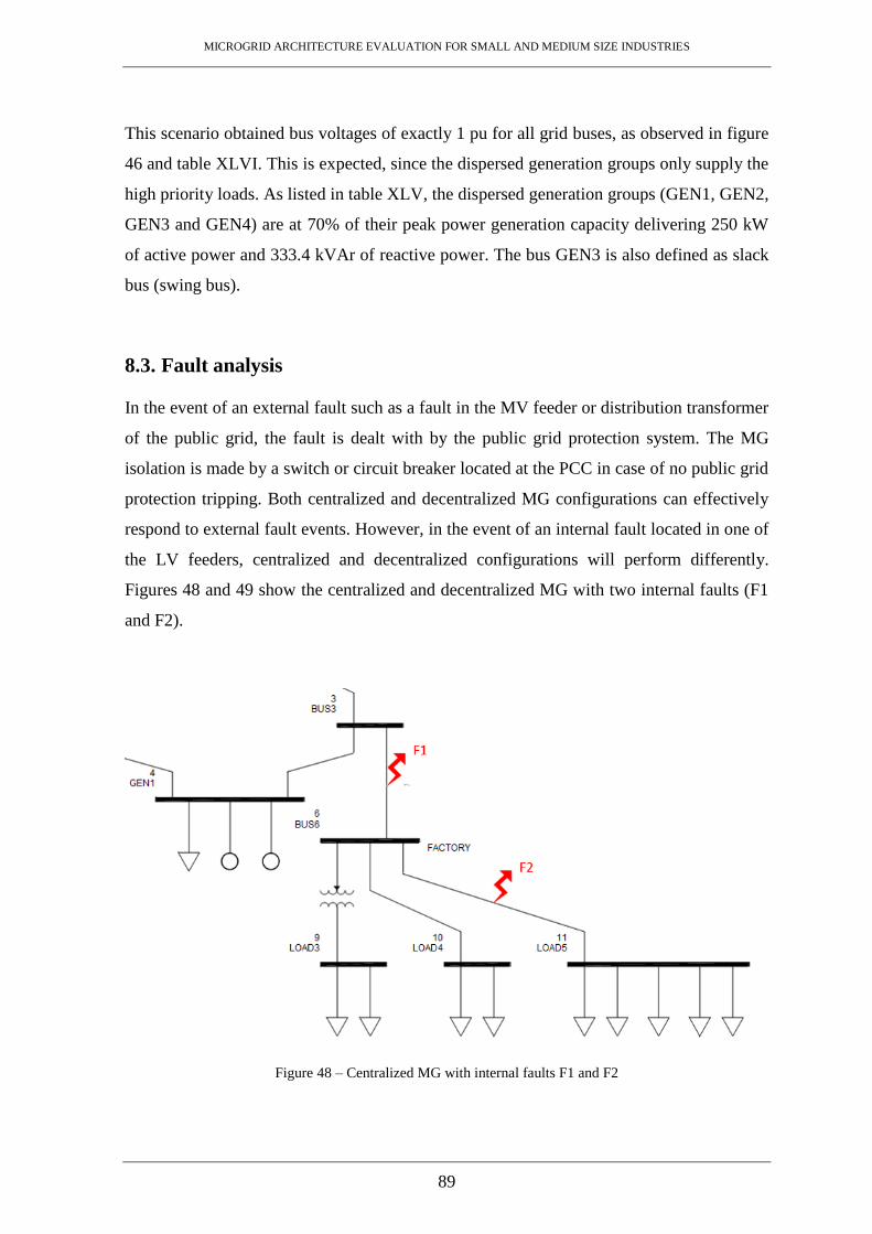
MICROGRID ARCHITECTURE EVALUATION FOR SMALL AND MEDIUM SIZE INDUSTRIES
89
This scenario obtained bus voltages of exactly 1 pu for all grid buses, as observed in figure
46 and table XLVI. This is expected, since the dispersed generation groups only supply the
high priority loads. As listed in table XLV, the dispersed generation groups (GEN1, GEN2,
GEN3 and GEN4) are at 70% of their peak power generation capacity delivering 250 kW
of active power and 333.4 kVAr of reactive power. The bus GEN3 is also defined as slack
bus (swing bus).
8.3. Fault analysis
In the event of an external fault such as a fault in the MV feeder or distribution transformer
of the public grid, the fault is dealt with by the public grid protection system. The MG
isolation is made by a switch or circuit breaker located at the PCC in case of no public grid
protection tripping. Both centralized and decentralized MG configurations can effectively
respond to external fault events. However, in the event of an internal fault located in one of
the LV feeders, centralized and decentralized configurations will perform differently.
Figures 48 and 49 show the centralized and decentralized MG with two internal faults (F1
and F2).
Figure 48 – Centralized MG with internal faults F1 and F2
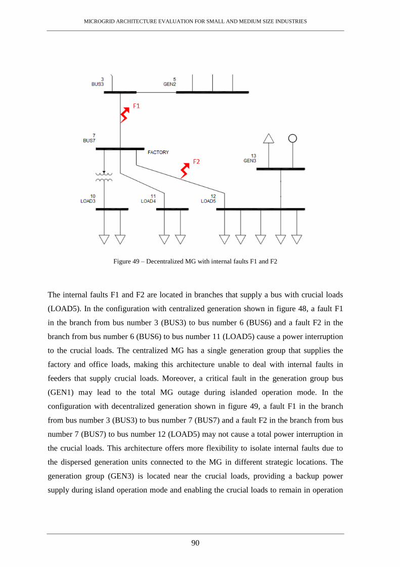
MICROGRID ARCHITECTURE EVALUATION FOR SMALL AND MEDIUM SIZE INDUSTRIES
90
Figure 49 – Decentralized MG with internal faults F1 and F2
The internal faults F1 and F2 are located in branches that supply a bus with crucial loads
(LOAD5). In the configuration with centralized generation shown in figure 48, a fault F1
in the branch from bus number 3 (BUS3) to bus number 6 (BUS6) and a fault F2 in the
branch from bus number 6 (BUS6) to bus number 11 (LOAD5) cause a power interruption
to the crucial loads. The centralized MG has a single generation group that supplies the
factory and office loads, making this architecture unable to deal with internal faults in
feeders that supply crucial loads. Moreover, a critical fault in the generation group bus
(GEN1) may lead to the total MG outage during islanded operation mode. In the
configuration with decentralized generation shown in figure 49, a fault F1 in the branch
from bus number 3 (BUS3) to bus number 7 (BUS7) and a fault F2 in the branch from bus
number 7 (BUS7) to bus number 12 (LOAD5) may not cause a total power interruption in
the crucial loads. This architecture offers more flexibility to isolate internal faults due to
the dispersed generation units connected to the MG in different strategic locations. The
generation group (GEN3) is located near the crucial loads, providing a backup power
supply during island operation mode and enabling the crucial loads to remain in operation
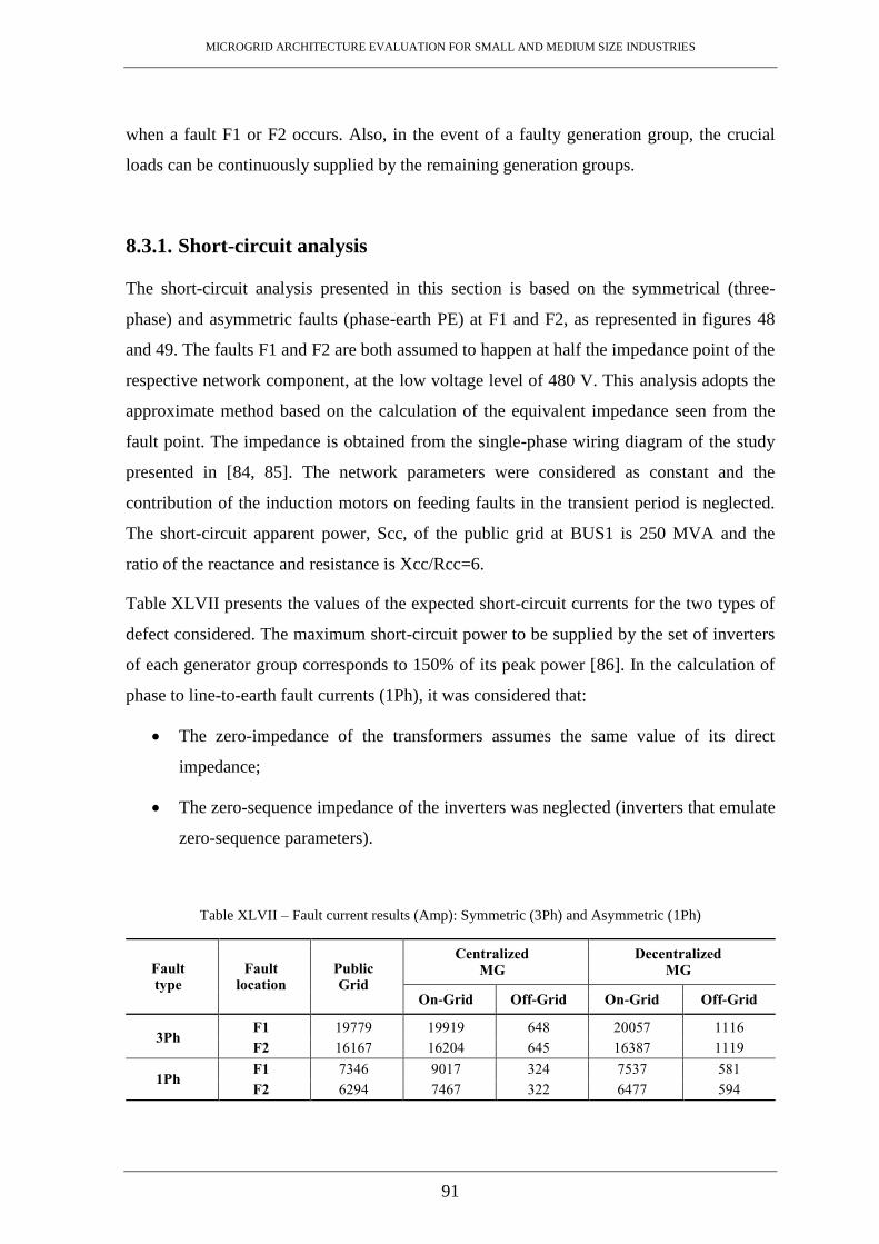
MICROGRID ARCHITECTURE EVALUATION FOR SMALL AND MEDIUM SIZE INDUSTRIES
91
when a fault F1 or F2 occurs. Also, in the event of a faulty generation group, the crucial
loads can be continuously supplied by the remaining generation groups.
8.3.1. Short-circuit analysis
The short-circuit analysis presented in this section is based on the symmetrical (three-
phase) and asymmetric faults (phase-earth PE) at F1 and F2, as represented in figures 48
and 49. The faults F1 and F2 are both assumed to happen at half the impedance point of the
respective network component, at the low voltage level of 480 V. This analysis adopts the
approximate method based on the calculation of the equivalent impedance seen from the
fault point. The impedance is obtained from the single-phase wiring diagram of the study
presented in [84, 85]. The network parameters were considered as constant and the
contribution of the induction motors on feeding faults in the transient period is neglected.
The short-circuit apparent power, Scc, of the public grid at BUS1 is 250 MVA and the
ratio of the reactance and resistance is Xcc/Rcc=6.
Table XLVII presents the values of the expected short-circuit currents for the two types of
defect considered. The maximum short-circuit power to be supplied by the set of inverters
of each generator group corresponds to 150% of its peak power [86]. In the calculation of
phase to line-to-earth fault currents (1Ph), it was considered that:
The zero-impedance of the transformers assumes the same value of its direct
impedance;
The zero-sequence impedance of the inverters was neglected (inverters that emulate
zero-sequence parameters).
Table XLVII – Fault current results (Amp): Symmetric (3Ph) and Asymmetric (1Ph)
Fault type
Fault location
Public Grid
Centralized MG
Decentralized MG
On-Grid Off-Grid On-Grid Off-Grid
3Ph F1 19779 19919 648 20057 1116
F2 16167 16204 645 16387 1119
1Ph F1 7346 9017 324 7537 581
F2 6294 7467 322 6477 594
MICROGRID ARCHITECTURE EVALUATION FOR SMALL AND MEDIUM SIZE INDUSTRIES
92
The analysis of this table shows that:
Symmetric and asymmetric faults generate significant currents whenever the
installation is connected to the public grid (On-Grid mode). The fault currents
increase slightly with the integration of the generator groups (Centralized MG /
Decentralized MG);
Symmetrical short-circuit currents for MGs in island mode are substantially low. In
Centralized MG, these fault currents are around 1.4 times the normal current at
rated load (Is). In Decentralized MG, these fault currents are around 2.4×Is;
Asymmetric faults, Ph-PE, in MGs in island mode generate very low currents. For
example, in the case of Centralized MG these currents correspond to about 0.85 of
Is (at fault F2) and in Decentralized MG are around 1.3×Is (at fault F1).
Thus it is possible to say that the regulation of short-circuit protections in MGs operating
in grid-connected mode is relatively straight-forward. On another hand, the regulation of
short-circuit protections in islanded MGs is quite more difficult.
8.4. Comments
In scenarios where the MG is in grid-connected operation mode, the public grid acts as a
generator connected to the slack or swing bus (SWING/BUS1) and it balances the active
and reactive power by setting the voltage angle reference for all MG buses. When the MG
is disconnected from the public grid (case 4C/4D and 5C/5D) and there is no slack or
swing bus available, the MG bus connected to the generator with the largest capacity
becomes the new swing bus and it is now responsible for regulating the active and reactive
power. Given the small proportions of the industrial grid studied, the voltage and angle
values obtained for each bus do not vary much between the different scenarios and it is
merely a result of a decrease in load demand. This can be easily observed in the islanded
operation scenarios (case 4C/4D and 5C/5D), there is an improvement in the bus voltage
profiles for both MG configurations because only the crucial loads are being supplied.

MICROGRID ARCHITECTURE EVALUATION FOR SMALL AND MEDIUM SIZE INDUSTRIES
93
Besides, it is noticeable few variations between the results obtained from the centralized
MG and decentralized MG configurations. When comparing the bus voltage profiles in
every scenario, the MG with dispersed generation groups obtained slightly better results
than the MG with a single generation group. As expected, the decentralized MG provides
better quality of supplied power to the loads with slightly better bus voltage profiles, since
there are generation groups dispersed along the grid and located near the crucial and most
demanding loads. Moreover, the decentralized MG configuration also provides flexibility
to isolate faults in branches that supply crucial loads and ensures the continuous power
supply in the event of a faulty generation group. On the other hand, there is bi-directional
power flow in the decentralized MG configuration, which increases the protection system
requirements. The centralized MG configuration is slightly simpler to implement and
requires less protection devices, but it does not provide the flexibility required to ensure
the continuous operation of crucial loads during islanded mode. Figure 50 represents the
schematics of the industrial MG with centralized and decentralized generation.
Figure 50 – Schematic of the industrial MG: A) centralized and B) decentralized
Table XLVIII shows a brief comparison between the two architecture configurations based
on the aspects previously mentioned in this section.

MICROGRID ARCHITECTURE EVALUATION FOR SMALL AND MEDIUM SIZE INDUSTRIES
94
Table XLVIII – Comparison between centralized and decentralized generation
Advantages Disadvantages
Centralized
Simple and less expensive
implementation
Less protection devices and
power converter interfaces
Difficulty in isolating internal
faults
Decentralized
Increased power quality and
less transmission losses
Flexibility to isolate internal
faults
High protection requirement due
to bi-directional power flow
MICROGRID ARCHITECTURE EVALUATION FOR SMALL AND MEDIUM SIZE INDUSTRIES
95
9. CONCLUSIONS
This work addressed some of the most important aspects to assist in the study of industrial
MG architectures. These aspects included a brief overview of the industrial sector and
definition of the MG concept, as well as a characterization of control and communication
architectures, energy resources, control strategies for power converters and protection
systems in MGs. The overview of the industrial sector focused on the challenge of
implementing energy efficiency measures in SMEs due to their limited financial resources
and lack of knowledge regarding cost-efficient applications of RES. Taking this into
account, implementing MGs in small scale enterprises might not be an easy and simple
task to accomplish, given the innumerable barriers these enterprises come across. Both the
control and communication architectures can follow a centralized or decentralized
configuration. There are economic concerns associated with the architecture configuration,
because a centralized approach proposes simpler and thus cheaper local control devices,
and also a central controller in charge of processing data and making decisions. A
decentralized approach requires more advanced and complex local control devices,
increasing the system cost. Moreover, the communication architecture may follow a wired
or wireless infrastructure based on a wide range of wired or wireless technologies with
different characteristics. The choice of an appropriate communication technology for a MG
must be according to the installation costs and system specifications. Environmental
concerns led to the deployment of several types of clean energy sources in MGs. The
overview of these energy sources mainly focused on solar and wind power generation
systems. PV technologies have been through a decrease in module prices and offer a long
service life with low operation costs, but the availability of PV and wind power systems is
dependent on the location and weather conditions. It is suggested the integration of hybrid
generation systems into the grid to ensure the continuous power supply and thus overcome
the dependency problem of PV and wind power systems. Most of the energy sources
require power converter interfaces to connect with the grid and these power converters
may follow different control strategies. The master-slave approach might not be suited for

MICROGRID ARCHITECTURE EVALUATION FOR SMALL AND MEDIUM SIZE INDUSTRIES
96
systems with dispersed generation, since a higher communication requirement is needed.
The multi-master approach provides an increase in reliability and allows simple system
expansion. An effective protection system is important to ensure a safe MG operation, as
well as the safety of crucial loads, generation sources, storage units and people. The
overview of the protection systems for feeders, buses and generation units focused on the
differential protection, mainly because this strategy overcomes the problem caused by the
integration of intermittent generation units into the grid. The earthing protection systems
commonly adopted in LV distribution systems is also addressed. The study concluded that
among the available systems, TN-S is the preferred earthing system for MGs.
The case study of a small scale centralized and decentralized MG was made using the
PSS/E Xplore software from Siemens. Both MG architectures showed almost ideal bus
voltage results (approximately 1 pu) due to the small grid size. However, the bus voltage
profiles obtained from the power flow study showed relatively better results with the
decentralized MG. In addition, it concluded that a decentralized MG is more capable of
isolating internal faults without compromising the operation of the crucial loads, due to a
dispersed deployment of generation units along the grid and close to loads. However,
because of bi-directional power flow, the decentralized approach has a higher protection
requirement, increasing the system costs. Taking into account the financial limitations of
smaller enterprises, every increase in system cost needs to be carefully considered. In
contrast, a centralized approach is simpler and cheaper to implement, but it cannot isolate
internal faults without compromising the continuous operation of crucial loads. A
centralized deployment of the generation units might be the preferred solution for small
grids. With a significant increase in grid size and number of loads, a decentralized
deployment of several generation units along the grid may bring noticeable advantages in
flexibility and quality of supplied energy. Furthermore, the operation of MGs in island
mode can be problematic. It was shown that currents generated by symmetric and
asymmetric faults in island operation mode are substantially lower than in grid-connected
operation. Therefore, in situations of minimum short-circuit currents setting the right
protections is neither simple nor economical.

MICROGRID ARCHITECTURE EVALUATION FOR SMALL AND MEDIUM SIZE INDUSTRIES
97
Future work and additional notes:
This dissertation was based on the project report made for the first INDuGRID project
task, entitled “Evaluating Architectures of Industrial Microgrids”. Additional aspects from
two papers submitted to the ICEREGA’17 conference were also included in this work.
Both conference papers are available in Appendix B. In addition, research work was
developed regarding the second INDuGRID project task “Protocols for guaranteeing zero
net energy industries”, but it was left for future work due to its incomplete state.

MICROGRID ARCHITECTURE EVALUATION FOR SMALL AND MEDIUM SIZE INDUSTRIES
99
REFERENCES
[1] U. Salahuddin, A. Berthold, “Design and development of industrial microgrids”,
White paper ABB, 2015.
[2] W. Muneer, K. Bhattacharya and C. A. Canizares, “Large-Scale Solar PV
Investment Models, Tools and Analysis: The Ontario Case”, IEEE Transactions on
Power Systems, vol. 26, n. 4, pp. 2547-2555, Nov. 2011.
[3] C. Genao, A. St. Leger, “Insight into Demand Response and Photovoltaic Source
with Time of Day Pricing”, Proceedings of the 2012 PES Transmission and
Distribution Conference and Exposition, pp. 1-8, May 2012.
[4] International Energy Outlook 2016, U.S. Energy Information Administration, May
2016. [Available online: https://www.eia.gov/outlooks/ieo/pdf/0484(2016).pdf
(Accessed: 2017-02-24)]
[5] “Study on Energy Efficiency and Energy Saving Potential in Industry and on
Possible Policy Mechanisms”, ICF International, Dec 2015. [Available online:
https://ec.europa.eu/energy/sites/ener/files/documents/151201%20DG%20ENER%
20Industrial%20EE%20study%20-%20final%20report_clean_stc.pdf (Accessed:
2017-09-14)]
[6] “Small and Medium-sized Enterprises: Local Strength, Global Reach”,
Organisation for Economic Co-operation and Development (OECD), Jun. 2000.
[Available online: http://www.oecd.org/cfe/leed/1918307.pdf (Accessed: 2017-02-
01)]
[7] “Accelerating Energy Efficiency in Small and Medium-sized Enterprises”,
International Energy Agency (IEA), 2015. [Available online:
https://www.iea.org/publications/freepublications/publication/SME_2015.pdf
(Accessed: 2017-02-01)]
MICROGRID ARCHITECTURE EVALUATION FOR SMALL AND MEDIUM SIZE INDUSTRIES
100
[8] “Research to Access the Barriers and Drivers to Energy Efficiency in Small and
Medium Sized Enterprises”, UK Department of Energy & Climate Change, Nov.
2014. [Available online:
https://www.gov.uk/government/uploads/system/uploads/attachment_data/file/3929
08/Barriers_to_Energy_Efficiency_FINAL_2014-12-10.pdf (Accessed: 2017-02-
01)]
[9] M. Bröckl, J. Illman, L. Oja, I. Vehviläinen, “Energy Efficiency in Small and
Medium Sized Enterprises”, Nordic Council of Ministers, 2014.
[10] “World Energy Outlook Special Report: Energy and Climate Change”,
International Energy Agency (IEA), 2015. [Available online:
https://www.iea.org/publications/freepublications/publication/WEO2015SpecialRe
portonEnergyandClimateChange.pdf (Accessed: 2017-03-08)]
[11] “Demand Response as a Power System Resource”, Regulatory Assistance Project
(RAP), May 2013. [Available online: http://www.raponline.org/wp-
content/uploads/2016/05/synapse-hurley-demandresponseasapowersystemresource-
2013-may-31.pdf (Accessed: 2017-09-25)]
[12] “Empowering Customer Choice in Electricity Markets”, International Energy
Agency (IEA), Oct. 2011. [Available online:
https://www.iea.org/publications/freepublications/publication/Empower.pdf
(Accessed: 2017-09-26)]
[13] “Benefits of Demand Response in Electricity Markets and Recommendations for
Achieving Them”, U.S. Department of Energy, Feb. 2006. [Available online:
https://eetd.lbl.gov/sites/all/files/publications/report-lbnl-1252d.pdf (Accessed:
2017-09-26)]
[14] N. Hatziargyriou, “Microgrids: Architectures and Control”, Wiley-IEEE press,
2014.
[15] J. C. Vasquez, J. M. Guerrero, E. Gregorio, P. Rodriguez, R. Teodorescu, and F.
Blaabjerg, “Adaptive Droop Control Applied to Distributed Generation Inverters
Connected to the Grid”, Proceedings of the 2008 IEEE International Symposium on
Industrial Electronics, pp. 2420-2425, 2008.
MICROGRID ARCHITECTURE EVALUATION FOR SMALL AND MEDIUM SIZE INDUSTRIES
101
[16] J. C. Vasquez, J. M. Guerrero, A. Luna, P. Rodriguez, and R. Teodorescu,
“Adaptive Droop Control Applied to Voltage-Source Inverters Operating in Grid-
Connected and Islanded Modes”, IEEE Transactions on Industrial Electronics, vol.
56, no. 10, pp. 4088-4096, Oct. 2009.
[17] J. Kennedy, P. Ciufo, A. Agalgaonkar, “Intelligent Load Management in
Microgrids”, Proceedings of the 2012 IEEE Power and Energy Society General
Meeting, pp. 1-8, Jul. 2012.
[18] http://www.cleanspark.com/the-grid-perfection-a-new-microgrid-landscape-in-the-
making/
[19] S. M. Nosratabadi, R. A. Hooshmand, E. Gholipour, “A comprehensive review on
microgrid and virtual power plant concepts employed for distributed energy
resources scheduling in power systems”, Renewable and Sustainable Energy
Reviews, vol. 67, pp. 341-363, 2017.
[20] J. M. Guerrero, J. C. Vasquez, J. matas, L. G. de Vicuna and M. Castilha,
“Hierarchical Control of Droop-Controlled AC and DC Microgrids—A General
Approach Toward Standardization”, IEEE Transactions on Industrial Electronics,
vol. 58, no. 1, pp. 158-172, Jan. 2011.
[21] K. D. Brabandere, B. Bolsens, J. V. D. Keybus, A. Woyte, J. Driesen, R. Belmans,
“A Voltage and Frequency Droop Control Method for Parallel Inverters”, IEEE
Transactions on Power Electronics, vol. 22, no. 4, pp. 1107-1115, Jul. 2007.
[22] A. M. Bollman, “An Experimental Study of Frequency Droop Control in a Low-
Inertia Microgrid”, Master Thesis, University of Illinois, 2009.
[23] A. Bidram and A. Davoudi, “Hierarchical Structure of Microgrids Control System”,
IEEE Transactions on Smart Grid, vol. 3, no. 4, pp. 1963-1976, Dec. 2012.
[24] O. Palizban, K. Kauhaniemi, “Hierarchical control structure in microgrids with
distributed generation: Island and grid-connected mode”, Renewable and
Sustainable Energy Reviews, vol. 44, pp. 797-813, 2015.
[25] L. K. Siow. P. L. So, H. B. Gooi, F. L. Luo, C. J. Gajanayake, Q. N. Vo, “Wi-Fi
Based Server in Microgrid Energy Management System”, Proceedings of the 2009
IEEE Region 10 Conference, pp. 1-5, Jan. 2009.

MICROGRID ARCHITECTURE EVALUATION FOR SMALL AND MEDIUM SIZE INDUSTRIES
102
[26] S. Shukla, Y. Deng, S. Shukla, L. Mili, “Construction of a Microgrid
Communication Network”, IEEE Power Engineering Society Innovative Smart
Grid Technology Conference, pp. 1-5, Feb. 2014.
[27] A. Bani-Ahmed, L. Weber, A. Nasiri, H. Hosseini, “Microgrid Communications:
State of the Art and Future Trends”, Proceedings of the 3rd
International
Conference on Renewable Energy Research and Applications, pp. 780-785, Oct.
2014.
[28] P. P. Parikh, M. G. Kanabar, T. S. Sidhu, “Opportunities and Challenges of
Wireless Communications Technologies for Smart Grid Applications”, Proceedings
of the 2010 IEEE PES General Meeting, pp. 1-7, Jul. 2010.
[29] E. Ancillotti, R. Bruno, M. Conti, “The role of communication systems in smart
grids: Architectures, technical solutions and research challenges”, Computer
Communications, vol. 36, pp. 1665-1697, 2013.
[30] M. Kuzlu, M. Pipattanasomporn, S. Rahman, “Communication network
requirements for major smart grid applications in HAN, NAN and WAN”,
Computer Networks, vol. 67, pp. 74-88, 2014.
[31] V. C. Gungor, D. Sahin, T. Kocak, S. Ergut, C. Buccella, C. Cecati, G. P. Hancke,
“Smart Grid Technologies: Communication Technologies and Standards”, IEEE
Transactions on Industrial Informatics, vol. 7, no. 4, pp. 529-539, Nov. 2011.
[32] Z. Zhu, S. Lambothran, W. Chin, Z. Fan, “Overview of demand management in
smart grid and enabling wireless communication technologies”, IEEE Wireless
Communications, vol. 19, no. 3, pp. 48-56, Jun. 2012.
[33] A. Usman, S. H. Shami, “Evolution of Communication Technologies for Smart
Grids Applications”, Renewable and Sustainable Energy Reviews, vol. 19, pp. 191-
199, 2013.
[34] Z. Ding, W. J. Lee, “A Stochastic Microgrid Operation Scheme to Balance
Between System Reliability and Greenhouse Gas Emissions”, IEEE Transactions
on Industry Applications, vol. 52, no. 2, pp. 1157-1166, Mar. 2016.
[35] L. Mariam, M. Basu, M. F. Conlon, “A Review of Existing Microgrid
Architectures” Journal of Engineering, pp. 1-8, 2013.

MICROGRID ARCHITECTURE EVALUATION FOR SMALL AND MEDIUM SIZE INDUSTRIES
103
[36] F. Katiraei, R. Iravani, N. Hatziargyriou, A. Dimeas, “Microgrids Management”,
IEEE Power and Energy Magazine, vol. 6, no. 3, pp. 66-77, 2008.
[37] “Renewable Energy Technologies: Cost Analysis Series - Solar Photovoltaics”,
International Renewable Energy Agency (IRENA), vol. 1, no. 4, Jun. 2012.
[Available online:
https://www.irena.org/DocumentDownloads/Publications/RE_Technologies_Cost_
Analysis-SOLAR_PV.pdf (Accessed: 2017-04-10)]
[38] M. A. Green, K. Emery, Y. Hishikawa, W. Warta, E. D. Dunlop, D. H. Levi, A. W.
Y. Ho-Baillie, “Solar cell efficiency tables (version 49)”, Progress in
Photovoltaics, vol. 25, no. 1, pp. 3-13, Jan. 2017.
[39] http://www.trinasolar.com/us/resources/downloads
[40] H. Moradi, A. Abtahi, R. Messenger, “Annual Performance Comparison Between
Tracking and Fixed Photovoltaic Arrays”, Proceedings of the 2016 IEEE 43rd
Photovoltaic Specialists Conference, pp. 3179-3183, Jun. 2016.
[41] R. Bruno, P. Bevilacqua, L. Longo, N. Arcuri, “Small size single-axis PV trackers:
control strategies and system layout for energy optimization”, 70th Conference of
the ATI Engineering Association, vol. 82, pp. 737-743, Dec. 2015.
[42] http://solarpv4u.co.nz/triangle-tilt-mounting/system
[43] http://www.solar-motors.com/gb/solar-tracker-d487.shtml
[44] http://www.nrel.gov/analysis/tech_lcoe_re_cost_est.html
[45] https://www.brasit.pl/pionowa-elektrownia-wiatrowa-bof-v-5kw/
[46] https://www.rocketsolar.eu/air-30-wind-turbine.html
[47] http://www.windturbinestar.com/hawt-vs-vawt.html
[48] “Benchmarking of Small and Medium Size Wind Turbine Technologies and Legal
Framework”, Baltic Energy Conservation Agency (BAPE), Dec. 2013. [Available
online: http://swipproject.eu/wp-content/uploads/2015/11/D1.1_2.pdf (Accessed:
2017-03-20)].
[49] http://www.motorship.com/news101/engines-and-propulsion/wartsila-installs-sofc-
fuel-cell-unit-on-car-carrier
MICROGRID ARCHITECTURE EVALUATION FOR SMALL AND MEDIUM SIZE INDUSTRIES
104
[50] “Fuel Cells”, Institution of Engineering and Technology, 2009.
[51] “Transforming Power Generation and Enhancing the Resiliency of the Electric
Grid”, FuelCell Energy Annual Report, 2014. [Available online:
http://www.annualreports.com/HostedData/AnnualReportArchive/f/NASDAQ_FC
EL_2014.pdf (Accessed: 2017-03-15)]
[52] “Fuel Cells”, IEA Energy Technology Essentials, 2007.
[53] https://www.capstoneturbine.com/products/c200
[54] V. A. Boicea, “Essentials of Natural Gas Microturbines”, CRC Press, 2013.
[55] http://www.offgridenergy.com.au/batteries/
[56] K. C. Divya, J. Ostergaard, “Battery energy storage technology for power
systems—An overview”, Electric Power System Research, vol. 79, pp. 511-520,
2009.
[57] H. Chen, T. N. Cong, W. Yang, C. Tan, Y. Li, Y. Ding, “Progress in electrical
energy storage system: A critical review” Progress in Natural Science, vol. 19, no.
3, pp. 291-312, Mar. 2009.
[58] F. D. González, A. Sumper, O. G. Bellmunt, R. V. Robles, “A review of energy
storage technologies for wind power applications”, Renewable and Sustainable
Energy Reviews, vol. 16, pp. 2154-2171, 2012.
[59] R. Esche, “Safety of Flywheel Storage Systems”, White paper Stornetic, 2016.
[60] https://gigaom.com/2011/10/31/and-the-next-solyndra-is-beacon-power/
[61] S. Schoenung, “Energy Storage System Cost Update: A Study for the DOE Energy
Storage Systems Program”, Sandia National Laboratories, 2011.
[62] http://www.windpowerengineering.com/design/electrical/ultracap-bank-capable-of-
discharging-1-mw-for-60-sec/
[63] http://www.maxwell.com/products/ultracapacitors/modules
[64] I. Kougias, S. Szabó, F. M. Ferrario, T. Huld, K. Bódis, “A methodology for
optimization of the complementarity between small-hydropower plants and solar
PV systems”, Renewable Energy, vol. 87, pp. 1023-1030, 2016.
MICROGRID ARCHITECTURE EVALUATION FOR SMALL AND MEDIUM SIZE INDUSTRIES
105
[65] M. Surprenant, I. Hiskens, G. Venkataramanan, “Phase Locked Loop Control of
Inverters in a Microgrid”, Proceedings of the 2011 IEEE Energy Conversion
Congress and Exposition, Sep. 2011.
[66] I. Patrao, R. González-Medina, S. Marzal, G. Garcerá, E. Figueres,
“Synchronization of power converters in islanded microgrids using an FM-
modulated signal”, IEEE Transactions on Smart Grid, vol. 8, no. 1, pp. 503-510,
Jan. 2017.
[67] J. Rocabert, A. Luna, F. Blaabjerg, and P. Rodriguez, “Control of Power Converters
in AC Microgrids”, IEEE Transactions on Power Electronics, vol. 27, no. 11, pp.
4734-4739, Nov. 2012.
[68] A. Vinayagam, K. S. V. Swarna, S. Y. Khoo, A. T. Oo, A. Stojcevski, “PV Based
Microgrid with Grid-Support Grid-Forming Inverter Control-(Simulation and
Analysis)”, Smart Grid and Renewable Energy, vol. 8, no. 1, pp. 1-30, Jan. 2017.
[69] J. A. P. Lopes, C. L. Moreira, and A. G. Madureira, “Defining Control Strategies
for Microgrids Islanded Operation”, IEEE Transactions on Power Systems, vol. 21,
no. 2, pp. 916-924, May 2006.
[70] M. S. Mahmoud, “Microgrid: Advanced Control Methods and Renewable Energy
System Integration”, 2016.
[71] G. Buigues, A. Dysko, V. Valverde, I. Zamora, E. Fernández, “Microgrid
Protection: Technical challenges and existing techniques”, International
Conference on Renewable Energies And Power Quality (ICREPQ’13), no. 11, Mar.
2013.
[72] H. Nikkhajoei, R. H. Lasseter, “Microgrid Protection”, Proceedings of the 2007
IEEE PES General Meeting, pp. 1-6, Jun. 2007.
[73] ABB, “ANSI numbers”, IEEE Standard Electric Power System Device Function
Numbers acc. to IEEE C.37.2-1991, Jul. 1998.
[74] N. Jenkins, X. Wu, N. Jayawarna, Y. Zhang, J. P. Lopes et al, “Protection
guidelines for a microgrid”, CORDIS, pp. 1-370, 2005.

MICROGRID ARCHITECTURE EVALUATION FOR SMALL AND MEDIUM SIZE INDUSTRIES
106
[75] H. Al-Nasseri, M. A. Redfern, F. Li, “A voltage based protection for micro-grids
containing power electronic converters”, Proceedings of the 2006 IEEE Power
Engineering Society General Meeting, pp. 1-7, 2006.
[76] M. Dewadasa, A. Ghosh, G. Ledwich, “Distance protection solution for a converter
controlled microgrid”, Proceedings of the 15th
National Power Systems Conference,
pp. 1-661, Dec. 2008.
[77] M. Dewadasa, A. Ghosh, G. Ledwich “Protection of Microgrids Using Differential
Relays”, Proceedings of the 2011 21st Australasian Universities Power Engineering
Conference, pp. 1-6, Sep. 2011.
[78] A. A. Memon, K. Kauhaniemi, “A critical review of AC Microgrid protection
issues and available solutions”, Electric Power System Research, vol. 129, pp. 23-
31, 2015.
[79] A. R. Haron, A. Mohamed, H. Shareef, “A Review on Protection Schemes and
Coordination Techniques in Microgrid System”, Journal of Applied Sciences, vol.
12, pp. 101-112, 2012.
[80] L. BoTong, L. YongLi, M. Tao, “Research on earthing schemes in LV microgrids”,
Proceedings of the 2011 International Conference on Advanced Power System
Automation and Protection, pp. 1003-1007, Oct. 2011.
[81] R. M. Kamel, A. Chaouachi, K. Nagasaka, “Comparison the Performances of Three
Earthing Systems for Micro-Grid Protection during the Grid Connected Mode”,
Smart Grid and Renewable Energy, vol. 2, no. 3, pp. 206-215, Aug. 2011.
[82] A. Momeneh, M. Castilla, M. M. Ghahderijani, A. Camacho, L. G. Vicuña,
“Design and Control of a Small-Scale Industrial Microgrid in Islanding Mode”,
Proceedings of the 42nd
Annual Conference of the IEEE Industrial Electronics
Society, pp. 72-77, Oct. 2016.
[83] T. N. Boutsika, S. A. Papathanassiou, “Short-circuit calculations in networks with
distributed generation”, Elsevier, Electric Power Systems Research, pp. 1181-1191,
2008.
[84] ABB, “MV/LV transformer substations: theory and examples of short-circuit
calculation”, QT Technical Application Papers, Feb. 2008.

MICROGRID ARCHITECTURE EVALUATION FOR SMALL AND MEDIUM SIZE INDUSTRIES
107
[85] P. Piagi, R. H. Lasseter, “Industrial Applications of Microgrids”, Power System
Engineering Research Center, University of Wisconsin-Madison, 2001.
[86] T. Loix, T. Wijnhoven, G. Deconinck, “Protection of microgrids with a high
penetration of inverter-coupled energy sources. Integration of Wide-Scale
Renewable Resources into the Power Delivery System”, CIGRE/IEEE PES Joint
Symposium, vol. 1, no. 6, pp. 29-31, Jul. 2009.

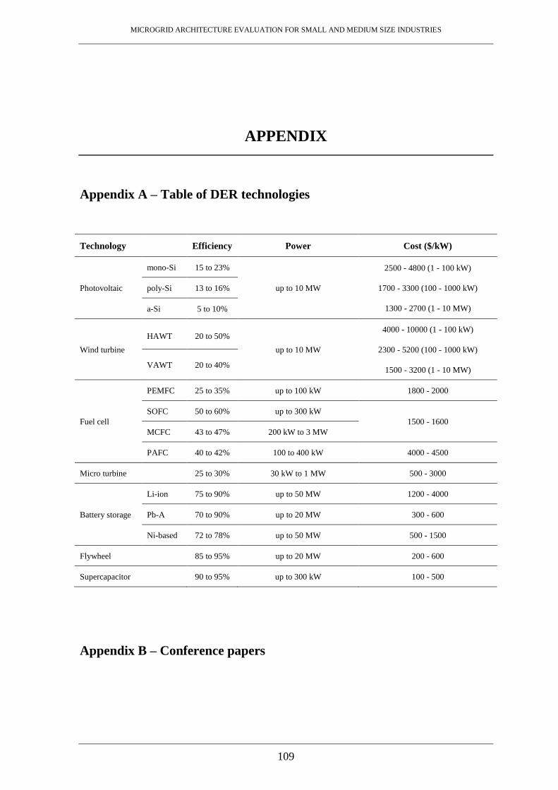
MICROGRID ARCHITECTURE EVALUATION FOR SMALL AND MEDIUM SIZE INDUSTRIES
109
APPENDIX
Appendix A – Table of DER technologies
Technology Efficiency Power Cost ($/kW)
Photovoltaic
mono-Si 15 to 23%
up to 10 MW
2500 - 4800 (1 - 100 kW)
1700 - 3300 (100 - 1000 kW)
1300 - 2700 (1 - 10 MW)
poly-Si 13 to 16%
a-Si 5 to 10%
Wind turbine
HAWT 20 to 50%
up to 10 MW
4000 - 10000 (1 - 100 kW)
2300 - 5200 (100 - 1000 kW)
1500 - 3200 (1 - 10 MW) VAWT 20 to 40%
Fuel cell
PEMFC 25 to 35% up to 100 kW 1800 - 2000
SOFC 50 to 60% up to 300 kW
1500 - 1600
MCFC 43 to 47% 200 kW to 3 MW
PAFC 40 to 42% 100 to 400 kW 4000 - 4500
Micro turbine 25 to 30% 30 kW to 1 MW 500 - 3000
Battery storage
Li-ion 75 to 90% up to 50 MW 1200 - 4000
Pb-A 70 to 90% up to 20 MW 300 - 600
Ni-based 72 to 78% up to 50 MW 500 - 1500
Flywheel 85 to 95% up to 20 MW 200 - 600
Supercapacitor 90 to 95% up to 300 kW 100 - 500
Appendix B – Conference papers