Microscopic Calabi-Yau Black Holes in String Theory · Microscopic Calabi-Yau Black Holes in String Theory Saeid Ansari ... Zusammenfassung In dieser Arbeit untersuchen wir mikroskospische

Microscopic Calabi-Yau Black holes in String Theory

Saeid Ansari

München 2011

Microscopic Calabi-Yau Black Holes in String Theory

Saeid Ansari

Dissertation an Fakultät Physik

der Ludwig-Maximilians-Universität München

vorgelegt von Saeid Ansari aus Teheran

München, den 1. Dezember 2010

Erstgutachter: Prof. Dr. Ivo Sachs

Zweitgutachter: Prof. Dr. Christian Römelsberger

Tag der mündlichen Prüfung: 22 Juli 2011

To my parents

Zusammenfassung

In dieser Arbeit untersuchen wir mikroskospische Aspekte von Schwarzen Löchernmit Calabi-Yau-Geometrie in Typ-IIA-Stringtheorie. Wir berechnen den Absorptionsquer-schnitt der masselosen Raumzeitskalare durch das D2-Branen-Weltvolumen, welches umeine S2 einer AdS2 × S2 ×CY3-Geometrie eines vier-dimensionalen Schwarzen Lochsmit Calabi-Yau-Geometry gewickelt ist. Die D2-Brane kann auch eine gewöhnliche D0-Probebranen-Ladung besitzen. Wir beschränken uns jedoch auf D2-Branen mit kleinerD0-Ladung, sodass Störungstheorie anwendbar ist. Der Kandidat für die duale Theo-rie gemäß der vorgeschlagenen AdS2/QM-Korrespondenz ist die Quantenmechanik einerMenge von D0-Probebranen in der AdS2-Geometrie. Für kleine aber von Null verschiedeneD0-Probeladungen finden wir den quantenmechanischen Absorptionsquerschnitt, der voneinem asymptotischen anti-de Sitter-Beobachter gesehen wird. Wir wiederholen die Rech-nungen für verschwindende D0-Probeladungen und diskutieren unser Ergebnis im Ver-gleich mit dem klassischen Absorptionsquerschnitt. In einem weiteren Projekt ermittelnwir für ein gegebenes vier-dimensionales Schwarzes Loch mit Calabi-Yau-Geometrie undgewöhnlichen D6-D4-D2-D0 Ladungen die Menge der supersymmetrischen Branen derkorrespondierenden elf-dimensionalen Geometrie in der Nähe des Horizonts, die in glob-alen Koordinaten statisch oder stationär sind. Die Menge dieser BPS-Zustände, die Branenmiteinschließt, die teilweise oder ganz den Horizont einhüllen, sollten für das Verständnisder Zustandssumme von Schwarzen Löchern mit D6-Ladungen von Bedeutung sein.

Abstract

In this thesis we study microscopic aspects of Calabi-Yau black holes in string theory.We compute the absorption cross-section of the space-time massless scalars by the world-volume of D2-branes, wrapped on the S2 of an AdS2 × S2 ×CY3 geometry of a four-dimensional D4-D0 Calabi-Yau black hole. The D2-brane can also have a generic D0probe-brane charge. However, we restrict ourselves to D2-branes with small D0-chargeso that the perturbation theory is applicable. According to the proposed AdS2/QM cor-respondence the candidate for the dual theory is the quantum mechanics of a set of probeD0-branes in the AdS2 geometry. For small but non-zero probe D0-charge we find the quan-tum mechanical absorption cross-section seen by an asymptotic anti-de Sitter observer. Werepeat the calculations for vanishing probe D0-charge as well and discuss our result bycomparing with the classical absorption cross-section. In other project, for a given four-dimensional Calabi-Yau black hole with generic D6-D4-D2-D0 charges we identify a set ofsupersymmetric branes, which are static or stationary in the global coordinates, of the cor-responding eleven-dimensional near horizon geometry. The set of these BPS states, whichinclude the branes partially or fully wrap the horizon, should play a role in understandingthe partition function of black holes with D6-charge.

Contents

1 Introduction 1

2 Black Holes in General Relativity 72.0.1 Schwarzschild black hole . . . . . . . . . . . . . . . . . . . . . . . 72.0.2 Reissner-Nordström black hole . . . . . . . . . . . . . . . . . . . . 8

2.1 Black hole thermodynamics and quantum aspects . . . . . . . . . . . . . . 112.2 Classical absorption on black holes . . . . . . . . . . . . . . . . . . . . . . 132.3 Computing the low energy absorption cross-section . . . . . . . . . . . . . 142.4 Absorption on 4D Schwarzschild black holes . . . . . . . . . . . . . . . . 15

2.4.1 Wave equation and the solution . . . . . . . . . . . . . . . . . . . 162.4.2 Matching the far and near solutions . . . . . . . . . . . . . . . . . 172.4.3 Computing absorption cross-section . . . . . . . . . . . . . . . . . 17

2.5 Absorption on 4D Reissner-Nordström black holes . . . . . . . . . . . . . 182.5.1 Extremal . . . . . . . . . . . . . . . . . . . . . . . . . . . . . . . 182.5.2 Near-extremal . . . . . . . . . . . . . . . . . . . . . . . . . . . . . 22

2.6 Universality of low energy absorption cross-section . . . . . . . . . . . . . 27

3 Black Holes in String Theory 313.1 Introduction . . . . . . . . . . . . . . . . . . . . . . . . . . . . . . . . . . 313.2 Calabi-Yau black holes in IIA . . . . . . . . . . . . . . . . . . . . . . . . 32

3.2.1 IIA string theory field content . . . . . . . . . . . . . . . . . . . . 323.2.2 D4-D0 Black hole . . . . . . . . . . . . . . . . . . . . . . . . . . 343.2.3 Branes in AdS2×S2×CY3 background geometry . . . . . . . . . . 37

3.3 Black holes entropy from string theory . . . . . . . . . . . . . . . . . . . . 413.3.1 Example: D4-D0 black hole on T 6 . . . . . . . . . . . . . . . . . . 43

3.4 Absorption of black holes in string theory . . . . . . . . . . . . . . . . . . 453.5 Absorption on horizon-wrapped branes . . . . . . . . . . . . . . . . . . . . 46

3.5.1 Vibration modes . . . . . . . . . . . . . . . . . . . . . . . . . . . 463.5.2 Absorption . . . . . . . . . . . . . . . . . . . . . . . . . . . . . . 493.5.3 Spherical excitations without D0-charge . . . . . . . . . . . . . . . 503.5.4 Spherical excitations with D0-charge . . . . . . . . . . . . . . . . 543.5.5 Dilaton with arbitrary angular momentum . . . . . . . . . . . . . . 553.5.6 Detailed calculation of absorption amplitude’s integral . . . . . . . 57

3.6 Discussion . . . . . . . . . . . . . . . . . . . . . . . . . . . . . . . . . . . 58

4 Supersymmetric Branes in Calabi-Yau Black hole 614.1 Introduction . . . . . . . . . . . . . . . . . . . . . . . . . . . . . . . . . . 614.2 Supersymmetric properties of the branes . . . . . . . . . . . . . . . . . . . 634.3 Supersymmetric branes in M-theory attractor geometries . . . . . . . . . . 65

4.3.1 Near horizon geometry of D6-D4-D2-D0 black holes . . . . . . . . 654.3.2 Global coordinates and half BPS-branes, five-dimensional analysis . 67

viii Contents

4.3.3 Half BPS M2-branes in global coordinates . . . . . . . . . . . . . 684.3.4 Half BPS five-branes . . . . . . . . . . . . . . . . . . . . . . . . . 71

4.4 Discussion . . . . . . . . . . . . . . . . . . . . . . . . . . . . . . . . . . . 77

5 Discussion and Conclusion 79

A Calabi-Yau spaces 81

B Useful identities for γ-matrices 83

C Anti-de Sitter space geometry 85

D Bessel function 87

Bibliography 89

CHAPTER 1

Introduction

One of the most fascinating objects that general relativity predicts are the black holes. Innature, black holes are formed from the collapse of gravitating matter. The simplest modelfor black hole formation involves a collapsing thin spherical shell of a massless matter. Ashell of photons with very small extension and total mass M provides an example.

Black holes are, roughly speaking, solutions of the equation of motion of Einstein’s theoryof General Relativity that exhibit a region of the space-time which one can not escape.More precisely, a black hole is an asymptotically flat space-time containing a region whichis not in the backward lightcone of the future time-like infinity. Classically, the black holesare completely black. Objects inside their event horizon are eternally trapped and nothingcan emerge from inside the event horizon to the outside. Even light rays are confined bythe gravitational force. In the early seventies, number of laws that govern the physics ofblack holes were established.In particular, it was found that there is a very close analogybetween these laws and the four laws of thermodynamics [1]. The black hole laws becomethat of the thermodynamics if one replaces the surface gravity κ of the black hole by thetemperature T of a body in thermal equilibrium, the area of the black hole A by the entropyS, the mass of the black hole M by the energy of the system E etc.

Considering thermodynamical behavior for the black holes, it is natural to wonder whetherthis formal similarity is more than just an analogy. Classically the identification betweenthe black hole mechanics and the laws of thermodynamics does not seem to have physicalcontent, because a classical black hole is just black and, therefore, the mass can only in-crease as matter falls through the horizon, it cannot radiate and therefore one should assigntemperature zero to it so that the interpretation of the surface gravity as temperature fails tobe correct. However, when the quantum effects are taken into account one can analyze theblack holes in the context of the quantum field theory in the curved space-time, where thematter is described by the quantum field theory while the gravity treated as a classical back-ground field, so-called the semi-classical approximation, of a full theory of the quantumgravity. In this framework it was discovered [1] that the black holes can emit (Hawking)radiation and consequently, can loses mass via Hawking radiation which allows to assignthe so-called Hawking temperature. This gives the Bekenstein-Hawking entropy as

Smacro =A4

(1.1)

On the other hand, the entropy is also a measure for the number of internal microstatesof the system. To compute the entropy on the microscopic side one needs to identify the

2 Chapter 1. Introduction

internal microstates and count the degeneracy N of microstates which give rise to a samemacrostate. The microscopic entropy is, accordingly, given by

Smicro = logN (1.2)

This raise the question about the nature of the microstates of a black hole. One would liketo understand whether there exists a fundamental, microscopic level describing the blackholes.

String theory, as the leading candidate for the quantum theory of gravity, should be able totell us about the microscopic configuration or, in other word, about the quantum statisticalmechanics of the black holes. The detailed study of matching the thermodynamic entropywith state counting in string theory is, however, only possible for the supersymmetric blackholes [2, 3]. These are the black holes that are asymptotically flat, charged and extremal,also called the BPS black holes. The key point is that as long as the supersymmetry ispreserved certain quantities can be calculated at zero coupling and the result remains validfor all values of the string coupling, gs. The BPS property, especially, ensures that thenumber of micro-states will be conserved under varying the coupling. Therefore, in case ofthe supersymmetric black holes, it is meaningful to count the microstates in non-interactingregime, where the coupling is zero, and compare it to the macroscopic entropy of blackhole, where the interactions are turned on.

Four Dimensional Physics

Since, string theory lives in a ten-dimensional space-time, or 11 dimensions from M-theorypoint of view, if we want to describe the four-dimensional black holes we should considera space-time where the extra dimensions have been compactified. With this assumption,the original ten-dimensional space-time would be split in two sub-spaces as

M4×X

where M4 is a four-dimensional space-time corresponding to the world we know, and Xis some compact six-dimensional manifold which is too small for us to observe directly.We can visualize this geometry by thinking that at every point in M4 there is correspondingspace X . Although, the compactified space can not be seen by the observers living in M, butproperties of the internal space X , lead to physical consequences in the four-dimensionalspace-time.

In principle, there are large number of possible six-dimensional compact manifolds onecould choose from, but, the requirement that the four-dimensional theory resemble theobserved world would limit our choice of X some what. Indeed, demanding that the su-persymmetry be preserved when we compactify our ten-dimensional theory to four di-mensions, lead us to the requirement that our compact space be a Calabi-Yau manifold.The Calabi-Yau manifolds are complex and are even-dimensional spaces which the six-dimensional one is called Calabi-Yau three-fold, briefly CY3. This leads us to the so-calledCalabi-Yau black holes in string theory.

3

The four-dimensional black holes in string theory are typically engineered in terms of thebranes wrapped around the appropriate cycles of the internal space [4].Suppose we have compactified the space-time, on a manifold, down to four dimensions,then the branes wrapped around the directions in the compact dimensions will look likepoint-like objects, or so to say (charged) particles, in the four-dimensional space-time,which are considered at a point in the space which is the center of black hole. Theseconfigurations have huge number of the internal excitations which all lead to a same four-dimensional black holes are count for the microscopic description.One of the special features of the supersymmetric black holes in four dimensions is thatthey have a residual supersymmetry and interpolate between two maximally supersymmet-ric vacua, namely the Minkowski space-time at infinity and the AdS2× S2 at the horizon.This lead us to the AdS2×S2×CY3 geometry at the near horizon of the Calabi-Yau blackhole. In more modern language, string theory in AdS background is conjectured to be dualto a conformal quantum mechanics [5], known as AdS/CFT correspondence. The AdS/CFTrelates a theory with gravity to theory without gravity [6]. In other word, the macroscopicgravitational dynamics are holographically encoded in the microscopic gauge theoreticaldegrees of freedom living at the conformal boundary of the near-horizon region.

This duality provide us a promising approach for reproducing the macroscopic entropy bystate counting, where for AdS2 is then AdS2/CFT1. In particular, it was shown [7] thatusing AdS2/CFT1 proposal for a class of black holes in IIA on the CY3 carrying D0 andD4-branes yield the result agrees with the Bekenstein-Hawking entropy formula, where theCFT1 takes the form of a quantum mechanics of a set of probe D0-branes moving in theAdS2 near-horizon geometry.

Apart from reproducing the entropy of the black hole one expects that the dual quantummechanics should also provide a microscopic description of the absorption- and Hawkingemission of the space-time fields by a black hole. This motivated us to compute the lowenergy absorption cross-section of the space-time scalars on an static D2-brane, wrappedon the S2 of an AdS2×S2×CY3 geometry [8]. In principle these D2-branes can also havea generic D0 probe-brane charge. However, for large probe D0-brane charge the couplingof the space-time fields to the world-volume quantum mechanics becomes large so that thelinearized perturbation theory is no longer applicable and back-reaction on the geometryhas to be taken into account.

Furthermore, though, the D4-D0 Calabi-Yau black hole and its dual quantum mechanicshave produced the results in agreement with the Bekenstein-Hawking entropy but since theD6-charge is taken to be zero, it is not the most general black holes we can construct in IIA.In general, we would like to get a precise microscopic description of the four dimensionalblack hole with all possible charges of IIA theory, namely non-vanishing D6-D4-D2-D0charges. Computing the entropy of such a CY3 black hole with generic charges and theirrelation to the conformal field theories are yet to be understood.

One can prepare the ground for extending the D4-D0 black hole to the black holes withD6-charge by describing the supersymmetric probe branes in the background of D6-charge.The classification of possible supersymmetric branes can play a role for understanding the

4 Chapter 1. Introduction

degeneracies of states, where will give some insight about the underlaying microscopictheory. This is the work done in our other project [9], where for a given black hole withgeneric D6-D4-D2-D0-charges in four dimensions, the set of supersymmetric branes, staticor stationary in global coordinates, of the corresponding eleven-dimensional near horizongeometry are identified.

This thesis is structured as follows: In chapter 2, first we review the black holes in gen-eral relativity, namely the Schwarzschild and the Reissner-Nordström black holes. We lookdeeper in case of the RN black hole and discuss its near horizon geometry. Then we addressthe thermodynamic laws of black holes, and specially the entropy. Since, we are interestedin the absorption of black holes, we provide the recipe of how to find the absorption cross-section for black holes and then we employ it to find the absorption cross-section for theSchwarzschild and Reissner-Nordström black holes. In case of RN we treat the absorp-tion for the extremal and the near-extremal case separately. In last section we review theuniversality of low energy absorption cross-section, namely the absorption cross-sectionindependency of the falling wave’s frequency. In chapter 3, we provide some backgroundof how to make a back hole in string theory. Specially we are interested in the Calabi-Yau black holes in IIA string theory with various wrapped-branes around the cycles of theCalabi-Yau. To do this we give the bosonic field content of IIA and then we talk about theD4-D0 black hole. As a simple example, we first illustrate the structure of the configurationof limited number of D4-branes and D0-branes in the context of toroidal compactifications,where the six-dimensional compact space is six-torus, T 6.We see that the near horizon ofsuch a class of black holes has an AdS2×S2 geometry. To have a better understanding ofthe possible brane interactions first we review the dynamics of the D-branes and their cou-pling to the various background fields. Specially we consider a D2-brane which is wrappedaround the horizon and couples to the background gauge field arising from the D4 and D0branes in the internal space. These branes can also have a D0-brane charge on them, weshow that the value of D0-charge determines the radial position of the D2-brane. Also weobserve that the horizon-wrapped branes are static in global coordinates while they pupout and in of the horizon in the Poincaré coordinates. After making a Calabi-Yau blackhole, we then address the entropy of black hole in string theory. The goal is to use stringtheory to reproduce the macroscopic entropy law by counting the states of the underlay-ing microscopic theory. We address why we are interested in the supersymmetric blackholes in string theory and then we give an example of how we count the degeneracy of ablack hole in the D-brane description. We consider three D4 branes where each of themare wrapped the four-cycles of six-torus plus some additional D0-branes and by countingthe degeneracies we lead to precise agreement between the macroscopic and microscopicblack hole entropy.

As the main part of the chapter we compute absorption of the space-time scalars by theworld-volume of D2-branes, wrapped on the S2 of a global AdS2×S2 geometry. The D2-branes can also have a generic D0 probe-brane charge. However, we will restrict ourselvesto the D2-branes with small D0-charge so that the perturbation theory is applicable. Firstwe identify the vibration modes of the brane then we compute the cross-section for theabsorption of dilatons on the two-brane. Starting with the s-wave absorption of the D2-

5

brane without any D0-charge, then we follow to find the absorption cross-section of higherpartial waves and also we compute the absorption on D2-brane in case of non-vanishingD0-charges. For small but non-zero probe D0-charge we find that the quantum mechan-ical absorption cross-section seen by an asymptotic anti-de Sitter observer, static in thePoincaré time vanishes linearly in ω for the small frequencies. We find the result which isin disagreement with the classical s-wave absorption cross-section by the black hole, whichvanishes quadratically in ω forthe small frequencies [10]. We will try to clarify this pointin the text.

Finally, in the last chapter we dealing with the problem of supersymmetric branes in theCalabi-Yau background. In this chapter we are interested in the possible supersymmetricM2 and M5-branes in M-theory which by the Calabi-Yau compactification give raise tofive-dimensions. To provide a base for our discussion, we start with describing the condi-tions which yield the BPS branes. In order to be self-contained and to fix the conventionswe first review the relevant static half BPS solutions of four-dimensional IIA supergrav-ity. Then, we will describe the eleven-dimensional near horizon geometry of a 4D blackhole with generic D6-D4-D2-D0 charge. We obtain the near horizon killing spinor in theglobal coordinates and analyze the κ-symmetry for stationary probe branes in the globaltime. In particular we find BPS two-branes wrapped on a two-cycle in the Calabi-Yau.Furthermore, we consider five-branes which can potentially wrap the horizon partially orcompletely. We determine the trajectories of the five-brane which preserve supersymme-try for the case of either wrap a holomorphic four-cycle in the Calabi-Yau and an S1 inspace-time (hence partially wrapping the horizon), or fully wrap the horizon S3/Zp0 and aholomorphic two-cycle in the Calabi-Yau. At the end we provide some useful material atthe appendices.

CHAPTER 2

Black Holes in General Relativity

Gravity, as a classical theory, is described by the Einstein classical theory of gravity. Thebasic idea of the Einstein gravity is that the geometry of space-time is dynamical and isdetermined by the matter distribution. Conversely the motion of matter is determined bythe space-time geometry. Einstein gravity without any sources, is based on the Einstein-Hilbert action

SEH =1

16πG

∫d4√−gR (2.1)

where G is the Newton gravitational constant. The classical equations of motion followingfrom this action are the source-free (Tµν ) Einstein equations

Gµν = Rµν −12

gµνR = 0 (2.2)

which comes from varying the action with respect to the metric. Here Rµν and R are theRicci tensor and the Ricci scalar, respectively. In case of presence of the matter coupled tothe gravity, the energy-momentum tensor is non-zero and so the Einstein equations wouldbe

Rµν −12

gµνR = 8πGTµν (2.3)

Some of the most interesting solutions to the equation of motion describe black holes.These solutions contains singularities at which certain curvature diverge.

The generalizations of the Einstein-Hilbert action are provided by considering the elec-tromagnetic fields, spinors or tensor fields, such as those that appear in the supergravitytheories. In case of the matter coupling to the electromagnetic field, which is relevant forus, one gets the, so called, Einstein-Maxwell action

S =∫

d4x√−|g|

(1

16πG4R− 1

4FµνFµν

)(2.4)

2.0.1 Schwarzschild black hole

The first exact solution to the Einstein’s equations of motion is the Schwarzschild solution,which describes a black hole. The Schwarzschild solution is the unique, spherically sym-metric and, by the Birkhoff’s theorem, static solution of the vacuum Einstein equation inthe four space-time dimensions.

8 Chapter 2. Black Holes in General Relativity

Solution to the vacuum, with a vanishing energy momentum tensor (Tµν = 0), Einstein’sequation is

Rµν = 0 (2.5)

that describes the geometry outside of the mass distribution which is precisely the Ricci-flat space-time. In the standard Schwarzschild coordinates (t,r,θ ,φ ) the Schwarzschildsolution is

ds2 = gµνdxµdxν =−(

1− rH

r

)dt2 +

(1− rH

r

)−1dr2 + r2dω

22 (2.6)

whererH = 2G4M (2.7)

is known as the Schwarzschild radius and G4 is the Newton’s constant.

dΩ22 = dθ

2 + sin2θdφ

2 (2.8)

is the metric of unit two-sphere. The surface r = rH is called the event horizon. Let us notethat rH is very small, for example one finds rH = 2.9km for the sun and rH = 9mm for theearth. Thus for atomic matter the Schwarzschild radius is inside the matter distribution andtherefore does not threat as a black hole. The Schwarzschild metric is only a function ofthe mass and it reduces to the Minkowski metric as the mass goes to zero. Furthermore themetric is asymptotically flat

gµν(r)r→∞−−−→ ηµν (2.9)

To see if M really has interpretation of a mass, we should consider the weak couplinglimit that is the asymptotic behavior of the metric. In general, in this limit the Newtonianpotential Φ in the stationary coordinates can be read off from the tt component of the metric

gtt ∼−(1−2Φ) (2.10)

So by taking r→ ∞ limit of the gtt component of the Schwarzschild black hole we have

gtt(r→ ∞)∼ 1− 2MG4

r(2.11)

which correctly produce the Newtonian potential

Φ =−2MG4

r(2.12)

2.0.2 Reissner-Nordström black hole

Generalization of the Schwarzschild black hole is the electrically charged one, which isknown as the Reissner-Nordström black hole.

9

An spherically symmetric solution of the coupled equations of the Einstein and of theMaxwell is the that of Reissner-Nordström. The Reissner-Nordström solution is the mostgeneral static black hole of the Einstein-Maxwell theory

S =∫

d4x√−|g|

(1

16πG4R− 1

4FµνFµν

)(2.13)

combined with the equation of motion and the Bianchi identity for the gauge field

∇µFµν = 0 (2.14)

εµνρσ

∂νFρσ = 0 (2.15)

The Einstein’s equations in the presence of an electric/magnetic field are

Rµν −12

gµνR = 8πG4

(FµρFρν

− 14

gµνFρσ Fρσ

)(2.16)

where Fµν denotes the components of Maxwell tensor. Taking the trace we get R = 0. Thisis always the case if the energy momentum tensor is traceless.The unique spherically symmetric solution of (2.16) is the Reissner-Nordström solution

ds2 =−∆dt2 +∆−2dr2 + r2dΩ

22

Ftr =−qr2 , Fθφ = psinθ (2.17)

∆ = 1− 2MG4

r+

(q2 + p2)G4

r2

q and p are the electric and magnetic charges of the black hole. This can be checked byrecalling the definition of electric and magnetic charge in terms of the Maxwell tensor

q =1

4π

∮∗F, p =

14π

∮F (2.18)

whereF =

12

Fµνdxµdxν (2.19)

is the two-form field strength , ∗F is the dual field strength and integration surface sur-rounds the sources. It is worthwhile to note that the solution is static and asymptoticallyflat.

The Reissner-Nordström black hole is characterized by three parameters, namely, the massM, the electric q and the magnetic charge p, where the charges can be conveniently com-bined into Q = q+ ip.The Reissner-Nordström metric has two horizons at

r = r± = MG4±√

(MG4)2−Q2G4 (2.20)

This encourage us to rewrite the metric in more convenient form as

ds2 = −∆+∆−dt2 +∆−1+ ∆

−1− dr2 + r2dΩ

22, (2.21)

∆± = 1− r±r


It should be clear that there is a singularity at r = 0. We have assumed that M ≥ Q, sinceotherwise there is no horizon and the solution has a naked singularity and thus is not phys-ically acceptable. This is known as the cosmic censorship hypothesis, which says that thegravitational collapse does not lead to a naked singularity. There is a very important specialcase arising when we saturate the lower bound on the mass, M, by making it equal to thecharge, Q, which is call the extremal case. Then we see that the both horizons coincide atr = Q. The extremal metric takes the form of

ds2 =−(

1− rH

r

)2dt2 +

(1− rH

r

)−2dr2 + r2dΩ

22 (2.22)

where rH = MG4. Let us change the radial coordinate to

y≡ r− rH (2.23)

then the metric can be written as

ds2ext =−H(y)−2dt2 +H(y)2(dy2 + y2dΩ

22), H(y)≡ 1+

rH

y(2.24)

which, now, the horizon is located at y = 0. We see that in these coordinates there is amanifest SO(3) symmetry. These are known as the isotropic coordinates.

2.0.2.1 Near horizon behavior

Another property of the extremal case, is when we are close to the horizon. Near thehorizon, where y≈ 0, the extremal metric (2.24) can be approximated by

ds2ext

y→0−−→−(

yrH

)2

dt2 +

(y

rH

)−2

dy2 + r2HdΩ

22 (2.25)

We see that the spatial part of the solution has degenerated into the product of an infinitelylong tube or ‘throat’of topologyR×S2 with fixed radius set by the value of horizon radius,or equivalently by the charge. The whole geometry, called the ‘Bertotti-Robinson’universe.Defining yet another coordinate as

z≡ r2H

r(2.26)

we find that the geometry approaches a direct product of a two sphere, parametrized by(θ ,φ) and a two-dimensional anti-de Sitter space parametrized by (r, t):

ds2ext =

r2H

z2 (−dt2 +dz2)︸︷︷︸+r2HdΩ

22︸︷︷︸ (2.27)

AdS2 × S2

The anti-de Sitter space-time is the most symmetric vacuum solution to the two-dimensionalEinstein equations with a negative cosmological constant.Both the sphere and the anti-de Sitter spaces have a same curvature radius, and becausethe AdS space has negative curvature, the curvature of full the metric is zero and so it isflat. Since the Reissner-Nordström space-time is also asymptotically flat, we see that itinterpolates between two maximally symmetric space-time.

2.1. Black hole thermodynamics and quantum aspects 11

2.1 Black hole thermodynamics and quantum aspects

One of the remarkable results of the black hole physics is that one can derive a set oflaws, called the laws of black hole mechanics, which have a same structure as the laws ofthermodynamics [11]. The black hole laws are derived using the geometrical properties ofevent horizon and has not linked to the thermodynamics from the beginning. The laws arestatements about the solution of the field equations, and in the original proofs the Einsteinequations are used.The zeroth black hole mechanics law states that the so-called surface gravity κ is constantover the event horizon of an stationary black hole.

κ = const. (2.28)

The surface gravity of an stationary black hole is the acceleration of an static observer atthe horizon, as measured by an observer at infinity).The first law is an energy conservation. It is simply an identity , relating the change in mass,M of an stationary black hole to the changes of the angular momentum, J, the horizon area,A, and the electric charge, Q,

δM =κ

8πδA+ΩHδJ+ΦHδQ (2.29)

where ΩH is the angular velocity at the horizon and ΦH is the electrostatic potential at thehorizon,ΦH = Q/rH .The second law says that the area of the horizon, A is non-decreasing function of time

δA≥ 0 (2.30)

The zeroth law of the black hole mechanics resembles the zeroth law of thermodynamics

T = 0 (2.31)

which says that the temperature is constant in a thermodynamic equilibrium, and also thefirst law of black hole has the same form as the first law of the thermodynamics

δE = T δS+ pdV +µdN (2.32)

The comparison of the first two laws suggests us to identify the surface gravity with thetemperature and consequently the area of horizon with the entropy

κ ∼ T , A ∼ S (2.33)

such that the temperature of black hole is its surface gravity and the entropy of black holeis equal to the size of the horizon. The analogy of the horizon area and the entropy isconfirmed by comparing the second law of black hole mechanics with the one from thethermodynamics.


Classically the identification between the black hole mechanics and the laws of thermody-namics does not seem to have a physical content, because a classical black hole is just blackand therefore, the mass can only increase as the matter falls through the horizon, it cannotradiate and therefore one should assign temperature zero to it, so that the interpretation ofthe surface gravity as a temperature has no physical content, since the surface gravity isnon-zero.However, when the quantum effects are taken into account one can analyze the black holesin the context of quantum field theory in a curved space-time, where matter is describedby the quantum field theory while gravity treated as a classical background field 1. In thisframework it was discovered [1] that the black holes can emit (Hawking) radiation. Hawk-ing argued that because the gravitational fields at the horizon are strong for a quantummechanical pair production in the vicinity of the horizon, one particle of the virtual pairfalls into the black hole and the other one is emitted as a radiation. Consequently, a blackhole can loses mass via the Hawking radiation 2. This allows us to assign the so-calledHawking temperature

TH =hκ

2π(2.34)

to a black hole, which is indeed proportional to the surface gravity. For example one cancompute the Hawking temperature for the sun, which is T ∼ 6×10−8K. Now we can lookat the first law. Since the Hawking temperature fixes the factor between temperature andsurface gravity, the entropy-area identification becomes precise

SBH =A

4hG4(2.35)

This relation is known as the area law and SBH is called the Bekenstein-Hawking entropy.We reinserted the Newton’s constant to show that the black hole entropy is dimensionless.

The area law is universally valid result for any black hole in any dimension

SBH =Ad

4Gd(2.36)

where Ad is the, (d−2)-dimensional, area of the horizon and Gd is the Newton’s constantin a d-dimensional space-time. Let us comment on the second law in the quantum realm.From one side, the Hawking radiation decreases the mass of the black hole and the horizonwill shrink. This violates the second law of the the black hole mechanics, which states thatthe area of the horizon is non-deceasing. On the other side, the classical second law ofthermodynamics violates because the entropy of black hole could be reduced by a mattermoving adiabatically, into the black hole. This contradiction, leads us to consider the, so-called, generalized entropy, which includes the entropy of black hole plus the other stuffsuch as the Hawking radiation and then, the second law of thermodynamics states that thetotal entropy is non-decreasing. One example of the unusual thermodynamic behavior of

1Of course, the quantum field theory in a curved space-time is only an approximation, so-called the semi-classical approximation, of a full theory of quantum gravity.

2Since, the radiation is thermal, the back-reaction can be neglected.

2.2. Classical absorption on black holes 13

the uncharged black hole is the dependence of temperature of the black hole to its mass.In case of the Schwarzschild black hole one finds T = 1/(8πM), which means that thespecific heat is negative and so the black hole heats up by loosing mass, till it fully decaysinto the radiation. This unusual behavior of the uncharged black holes leads to the informa-tion problem of quantum gravity. For the charged black holes, radiation can not destroysthe black hole, since it radiates till the extremality is reached. The Hawking temperaturevanishes in the extremal limit and therefore the extremal black holes are stable.Having established the thermodynamical laws for the black holes and knowing about themacroscopic parameters, one would like to understand the underlying microscopic theory,such as, where does the entropy of the black hole come from and what are the microscopicdegrees of freedom make up the black hole?In the other word, whether there exists a fundamental, microscopic level of black hole’sdescription, where one can identify the microstates and counts how many of them lead toa same macrostate. At the microscopic level one can define the microscopic or statisticalentropy by counting the degeneracy of microstates which give rise to a same macrostate.The macrostates of a black hole are characterized by its mass M, charge Q and angularmomentum J. Letting d(M,Q,J) be the number of the microstates of a black hole withmacroscopic parameters, M, Q, J, the microscopic black hole entropy is defined by

Smicro = log d(M,N,J) (2.37)

If the interpretation of the Bekenstein-Hawking entropy, SBH , as macroscopic entropy iscorrect, then it must be equal to the microscopic entropy, namely

SBH = Smicro (2.38)

We deal with the microscopical entropy in next chapter when we study the black holes instring theory.

2.2 Classical absorption on black holes

Let us look at the computation on the gravity side. Consider an spherical black hole with thehorizon area A. Suppose that we have a minimally coupled massless scalar in the theory:

Φ = 0 (2.39)

=1√−g

∂α

(√−ggαβ

∂β

)We wish to find the cross-section for absorption of such scalars into the black hole. To dothis, we must solve the wave equation (2.39), with some boundary conditions. We have aplane wave incident from infinity. We put the boundary condition at the horizon which saysthat the quanta are falling in but not coming out. Some part of the incident plane wave willbe reflected from the metric around the black hole and give rise to an outgoing waveformat infinity. The rest goes to the horizon and represents the part that is absorbed. From this


absorbed part we deduce the absorption cross-section σabs.In general, this is a hard calculation to do, but it becomes simple in the limit where thewavelength of the incident particle becomes much larger than the size of the black hole.We call this limit the low-energy absorption cross-section

ω 1M

(2.40)

To calculate the absorption cross-section we need to find the so-called greybody factor F

defined as

F =

∣∣∣∣ ftrfin

∣∣∣∣ (2.41)

where ftr and fin are, respectively, the flux passing the horizon and the incoming flux frominfinity. The greybody factor is an important quantity to understand the absorption andthe emission phenomena of a black hole. It is this factor which makes a black hole to bedifferent from a black body. The physical origin of this factor is the effective potentialbarrier generated by a black hole space-time. For example, the potential for the s-wavemassless scalar generated by a Schwarzschild space-time is

Ve f f (r∗) =rH

r3

(1− rH

r

)(2.42)

when the wave equation is expressed in terms of the “tortoise“ coordinate r∗= r+rH ln(r/rH−1). This potential generally backscatters a part of the outgoing radiation quantum me-chanically, which results a frequency-dependent greybody factor. To find the absorptioncross-section we need to project a plane wave into an s-wave. In four dimension, this gives

σabs =π

ω2 F (2.43)

2.3 Computing the low energy absorption cross-section

The computational procedure most people adopted is the matching procedure. In match-ing procedure we divide the space-time outside the horizon,r > rH , into two overlappingregions defined by

Near Horizon Region : r− rH 1ω

(2.44)

Far Region : M r− rH (2.45)

where in case of the RN black hole rH is the outer horizon. In each region the wave equation(2.39) can be approximated by using the above near horizon and far region properties andthen we can solve it exactly.Each of the, near horizon and far region, solutions would have undetermined coefficients.The complete solution obtained by fixing the constants and we find them by imposing theboundary conditions and by matching the solutions.

2.4. Absorption on 4D Schwarzschild black holes 15

To match the near and far solutions we take the large r limit of the near horizon solutionand match it to the small r limit of the far solution, namely

Φnh(r→ ∞) ⇔ Φ f ar(r→ 0) (2.46)

where Φnh and Φ f ar are, respectively, the near horizon and the far solutions of the waveequation. By matching the solutions we obtain a complete solutions of the wave equation.Now we can calculate the greybody factor, F . As already mentioned, the greybody factoris the ratio of the flux passing across the horizon, ftr to the incoming flux from infinity, fin

F =

∣∣∣∣ ftrfin

∣∣∣∣ (2.47)

and the conserved flux is defined as

f ≡ 4π

2i

√|g|grr (R∗(r)∂rR(r)−R∂rR∗) (2.48)

where r is for the radial coordinate and R(r) is the radial part of the wave equation Φ.We should notice that for computing the incoming flux from infinity, we must insert theincoming part of the Φ f ar in the flux equation. In case of the flux ingoing to the horizonwe have the boundary condition that the is no reflected wave and so we use the completeform of Φnr to determine the fin. Finally, we insert the computed greybody factor in (2.47)to find the absorption cross-section.In what follows we use the technique described here to calculate the absorption cross-section for massless scalars in case of the Schwarzschild and the Reissner-Nordström blackholes.

2.4 Absorption on 4D Schwarzschild black holes

As a first example we consider a four-dimensional Schwarzschild black hole and computethe absorption cross-section of a massless scalar.Absorption spectra of a Schwarzschild black hole firstly calculated in [12]. We look atthe low energy absorption, where only the mode with lowest angular momentum will con-tribute to the cross-section which for the scalars this is the s-wave.The Schwarzschild black hole metric is

ds2 =−h(r)dt2 +h(r)−1dr2 + r2dΩ22 h(r) := 1− rH

r(2.49)

where rH , the Schwarzschild radius, is related to the black hole mass M as

rH = 2M (2.50)

Now we follow the steps described in the previous section to calculate the absorption cross-section for the Schwarzschild black hole. First we should solve the wave equation (2.39)for the near horizon and asymptotic regimes.


2.4.1 Wave equation and the solution

The general form of the wave equation is

Φ(r, t) = 0 = ∂t

[√|g|gtt

∂t

]Φ(r, t)+∂r

[√|g|grr

∂r

]Φ(r, t) (2.51)

We adopt the separation of variation as

Φ(r, t) = e−iωtRω(r) (2.52)

With this, the wave equation would be

r2h(r)−1ω

2R(r)+∂r[r2h(r)∂r

]R(r) = 0 (2.53)

Next, we should solve the above wave equation in near horizon and far regions.

Far region

In the region far from the black hole, r→ ∞, the black hole and its effects disappear. Wehave

h(r)' 1 r→ ∞ (2.54)

and so the metric becomes a flat metric

ds2 =−dt2 +dr2 + r2dΩ22 (2.55)

thus the wave equation is simply

r2∂

2r R f ar(r)+2r∂rR f ar(r)+(rω)2R(r) = 0 (2.56)

where we have added the index "far“ to R(r) to remember that we are looking at the solutionof wave equation in the far region. Above differential equation has a complete solution inthe form of Bessel functions

R f ar(r) =√

π

2ωr

[αJ 1

2(ωr)−βJ− 1

2(ωr)

](2.57)

α and β are constants and J is Bessel function.

Near horizon

To solve the wave equation in the region close to the horizon, r→ rH , we define a newradial coordinate as

y :=1

rHln(h(r)) (2.58)

which simplifies the wave equation to

∂2y Rnh(y)+ rH

4ω

2Rnh(y) = 0 (2.59)

Solution to the above equation is

Rnh(y) = Ae−iωrH2y (2.60)

A is a constant which will be related to the constants in (2.57) when we match the solutions.

2.4. Absorption on 4D Schwarzschild black holes 17

2.4.2 Matching the far and near solutions

Now we must match the far and near solutions or more precisely we should match the nearhorizon solution when r→ ∞ to the far region solution when r→ 0.First, we look at the far region solution eq. (2.57) and take the r→ 0 limit, which is easilycarried out by using the series expansion of the Bessel functions 3

R f ar(r→ 0)' 1√r

[α

(ωr2

) 12 1

Γ(3

2

) +β

(ωr2

)− 12 1

Γ(1

2

)] (2.61)

For r→ ∞ limit of the near horizon solution we notice that

r→ ∞⇒ h(r)→ 1⇒ y→ 0 (2.62)

so (2.60) can be approximated by

Rnh(y→ 0)' A[1− iωr2Hy] (2.63)

or equally

Rnh(r→ ∞)' A[1− iωrH ln

(1− rH

r

)]' A(1+ iω

r2H

r) (2.64)

Now by comparing (2.61) and (2.64) we straightforwardly lead to

α =

(2ω

π

) 12

A (2.65)

β = ir2H

(πω3

2

) 12

A (2.66)

Also, since we are looking at the low energy limit where ω 1, we find that β α , whichwill use it later.

2.4.3 Computing absorption cross-section

To compute the absorption cross-section we need to know the incoming flux from infinityand the flux transmitted to the horizon. First, we compute the incoming flux from infinity,fin.In the far region, for r→∞ we can approximate the solution (2.57) by using the asymptoticform of the Bessel functions

R f ar(r→ ∞)' π

2ωr[sinωr+ cosωr] (2.67)

we need to compute the incoming flux, thus we should extract the incoming part of thewave equation. The above Bessel function can be rewritten as

R f ar(r→ ∞)' π

2ωr12[(iα +β )e−iωr(−iα +β )eiωr] (2.68)

3see appendix D there you can find more about Bessel functions and some useful formula.


this is of the form ofR f ar(r→ ∞) = φin +φre f (2.69)

where φin and φre f are, respectively, the incident and the reflected waves at infinity

φin =π

2ωr12(iα +β )e−iωr (2.70)

φre f =π

2ωr12(−iα +β )eiωr (2.71)

Now we have the incident part of the wave equation at infinity and we can compute theincoming flux from infinity by inserting φin in the definition of conserved flux (2.48)

fin(r→ ∞) =2π

ir2 [φ ∗in∂rφin−φin∂rφ

∗in] (2.72)

= 2(|α|2 + |β |2) (2.73)

where we have used the asymptotic form of the metric in far region (2.4.1). Also, since weare looking at the low energy limit where ω 1, according to (2.57) we find that β α

and so we can neglect the second term. Finally, the incoming flux from infinity is

fin(r→ ∞)' 2|α|2 (2.74)

The flux passing the horizon, fabs can be computed in a similar way.

fabs = 4πωrHA2 (2.75)

So by taking (2.70) the absorption cross-section found to be

σabs =π

ω2

∣∣∣∣ ftrfin

∣∣∣∣= 4πr2H = AH (2.76)

The absorption cross-section of the low energy massless scalars equals the area of thehorizon.

2.5 Absorption on 4D Reissner-Nordström black holes

Our next and more realistic example is the Reissner-Nordström black hole in a four-dimensionalspace-time. Again, we look at the absorption of a minimally coupled massless scalar. Weconsider the extremal and the near-extremal Reissner-Nordström separately and calculatethe absorption cross-section for each of them.

2.5.1 Extremal

The metric of an extremal Reissner-Nordström black hole is

ds2 =−(

1− rH

r

)2dt2 +

(1− rH

r

)−2dr2 + r2dΩ

2 (2.77)

2.5. Absorption on 4D Reissner-Nordström black holes 19

which for later convenience we define a new radial coordinate as

r = r− rH (2.78)

and dropping the tilde, then the metric transforms to

ds2 =−(

1+rH

r

)−2dt2 +

(1+

rH

r

)2 (dr2 + r2dΩ2

2) (2.79)

Now the horizon is located at zero rH = 0.which dΩ2

2 is the metric of an unit two-dimensional sphere.

Near horizon geometry

In the near horizon regime we can approximate the metric (2.79) as

ds2nh =−

(rH

r

)−2dt2 +

(rH

r

)2dr2 + rH

2dΩ22 (2.80)

which ds2nh stands for the near horizon metric. Again we change the radial coordinate as

rH

r= y (2.81)

then the metric simplifies as

dsnh2(y) =− 1

y2 dt2 +rH

2

y2 dy2 + rH2dΩ2

2 (2.82)

Wave equation and the solution

By inserting (2.79) in the wave equation, the radial part would be

∂r[r2

∂rR(r)]− l(l +1)R(r)− r2

ω2R(r) = 0 (2.83)

where we have assumed separability condition

Φ = e−iωtR(r)Yl(Ω) (2.84)

Yl(Ω) is spherical harmonics following

r2∇

2Yl(Ω) =−l(l +1)Yl(Ω) (2.85)

Now we look at the asymptotic and the near horizon form of the wave equation and alsowe find the solution for these regions.


Near horizon

To compute the wave equation for the near horizon we use the metric (2.82), the result ofradial part would be

Φ = ∂y2 +(rHω)2R(r)+

1y2 l(l +1)Rnh(y) = 0 (2.86)

Rnh(r) denotes the near horizon version of R(r). Above equation is a Bessel differentialequation and it has a complete solution as

Rnh(y) =√

y[AJl+ 1

2(rHωy)+BYl+ 1

2(rHωy)

](2.87)

or equally

Rnh(y) =√

y[AJl+ 1

2(rHωy)+BJ−l− 1

2(rHωy)

](2.88)

Far region

In the region far from the black hole, r 1, the black hole, and its effects, disappear andone leave with a flat metric

ds2f ar =−dt2 +dr2 + r2dΩ

22 (2.89)

using the flat metric, the wave equation would be

Φ(r, t) = ∂r[r2

∂rΦ(r, t)]−∂t

[r2

∂tΦ(r, t)]= 0 (2.90)

or∂

2r R(r)+2r∂rR(r)+(rω)2R(r) = 0 (2.91)

where we have assumed the separation of variables similar to the near-horizon case. Solu-tion to the above differential is, again, a linear combination of Bessel functions

R f ar(r) =1√r

[αJl+ 1

2(ωr)+βJ−l− 1

2(ωr)

](2.92)

we can simplify the solution by applying r→ ∞ to the solution. Then the solution behaveslike

R f ar(r)'1r

√2

πω

[α sin

(ωr− lπ

2

)+β cos

(ωr+

lπ2

)](2.93)

Matching the far and near solutions

As explained before, we need to match the small r far region solution (2.92) to the large r(y→ 0) near horizon solution (2.88). Using the series expansion of Bessel functions

Jα(x) =∞

∑m=0

(−1)m

m!Γ(m+α +1)

( x2

)2m+α

(2.94)


the asymptotic solution at small r (2.92) can be replaced by

R f ar(r→ 0)' 1√r

[α

(ωr2

)l+ 12 1

Γ(l + 3

2

) +β

(ωr2

)−l− 12 1

Γ(−l + 1

2

)] (2.95)

In the same way, the large r near horizon solution can be approximated by

Rnh(r→ ∞)' 1√r

[A(

ωrH2

r

)l+ 12 1

Γ(l + 3

2

) +B(

ωrH2

r

)−l− 12 1

Γ(−l + 1

2

)](2.96)

where we have resubstituted r from (2.81). Matching (2.95) at small r to (2.96) at large r,we get

α

Γ(l + 3

2

) (ωr2

)l+ 12

=B

Γ(−l + 1

2

) (ωrH2

r

)−l− 12

(2.97)

β

Γ(−l + 1

2

) (ωr2

)−l− 12

=A

Γ(l + 3

2

) (ωrH2

r

)l+ 12

(2.98)

In the low energy approximation (ω 1) one finds β α .

Computing absorption cross-section

To compute the absorption cross-section we need to know the incoming flux from infinityand the flux transmitted to the horizon. First, we compute the incoming flux from infinity,fin, by using the general form of the conserved flux associated to the wave equation (2.48).The Bessel function corresponding to the far region (2.93) can be writtien as

R f ar(r→ ∞)' 12r

√2

πω

[(−iα +β )e−i(ωr− lπ

2 ) +(iα +β )e+i(ωr− lπ2 )]

(2.99)

which can be decomposed into two terms as

R f ar(r→ ∞) = φin +φre f (2.100)

where φin and φre f are the incident and reflected waves, respectively. So, the incoming fluxfrom infinity can be derived as

fin =2π

ir2 (φ ∗in∂rφin−φin∂rφ

∗in)

= 2|α|2 +2|β |2

' 2|α|2 (2.101)

which in the last step we have used that α β . The flux passing across the horizon, fabs,can be computed by using the near horizon metric (2.80). For r→ 0, the Bessel function


(2.88) can be approximated by

Rnh(r→ 0) =

√1

πωrH

[Asin

(12(r2

Hω− lπ))+Bcos

(12(r2

Hω + lπ))]

=

√1

πωrH

[(−iA+B)e

−i(

ωr2H

r −lπ2

)+(iA+B)e

i(

ωr2H

r + lπ2

)](2.102)

First and second term in last line, are the transmitted and the reflected waves respectively.Demanding no reflection at the horizon, cause the restriction A =−iB. Now we can calcu-late the transmitted flux by using

φtr = (2B)e−i(

ωr2H

r −lπ2

)(2.103)

The result is thenfabs = 4|A|2 (2.104)

So the greybody factor, F , is

F =

∣∣∣∣ fabs

fin

∣∣∣∣= 2|B|2

|α|2= 2

∣∣∣∣∣Γ(−l + 1

2

)Γ(l + 3

2

) ∣∣∣∣∣2(

ωrH

2

)4l+2(2.105)

We can convert the partial wave cross-section to the plane wave cross-section by multiplyi-ing the above result by π/ω2. For s-wave, l = 0 we find

σ0abs = AH (2.106)

Absorption cross-section in the low energy limit is proportional to the area of the horizon.

2.5.2 Near-extremal

After dealing with the simple case of an extremal black hole, now we consider a general RNblack hole with no restriction on the charge. We follow a same procedure as the previoussection. As already mentioned, the complete RN metric is

ds2 =−∆dt2 +∆−1dr2 + r2dΩ

2 (2.107)

with∆ =

(1− r+

r

)(1− r−

r

)(2.108)

andr± = M±

√M2−Q2 (2.109)

Wave equation and the solution

By using the general form of wave equation we get[∂r∆∂r + r∆

−1∂

2t]

Φ = 0 (2.110)

We need to find the solution for above wave equation at the near horizon and far region,which will be done in the next two sections.


Near horizon

For the near horizon region we have

r− r+ 1ω

(2.111)

the wave equation can be written as

∆

r2 ∂r∆

r2 ∂rR+ω2r4

+−l(l +1)

r2 ∆R = 0 (2.112)

To solve the near horizon wave equation we define a new variable as

z =r− r+r− r−

, 06 z6 1 (2.113)

where z = 0 would be the horizon. The wave equation (2.110) becomes

0 = (r+− r−)z∂z(r+− r−)z∂zR+ω2r4

+R− l(l +1)(r− r+)(r− r−)R (2.114)

= (r+− r−)2z2∂

2z R+(r+− r−)2z∂zR+ω

2r4+R− l(l +1)(r− r+)(r− r−)R

and by dividing by z(r+− r−)(r− r−) we have

0 =r+− r−r− r−

z∂2z R− r+− r−

r− r−∂zR+

ω2r4+

z(r+−r−)(r− r−)R− l(l +1)

zr− r+

r+− r−R

= z(1− z)∂ 2z R+(1− z)∂zR+

ω2r4+

(r+− r−)2

(1− z

z

)R− l(l +1)

1− zR (2.115)

Above near horizon wave equation transforms into an standard hypergeometric form bydefining

R = Aziω r(1− z)l+1F , r :=r2+

r+− r−(2.116)

where A is a normalization constant which will be determined later.By applying above definition, F obeys

z(1− z)∂ 2z F +[1+ iω r− (1+2(l +1)+ iω r)z]∂zF−

[(l +1)2− iω r(l +1)

]F = 0

(2.117)

This is of the form of hypergeometric differential equation

z(1− z)∂ 2z F +[c− (a+b+1)z]∂zF−abzF = 0

with

a = l +1+ iωrr

b = l +1 (2.118)

c = 1+ iω r


(2.118) has following complete solution

F = A12F1(a,b;c;z)+A2z1−c2 F1(a+1− c,b+1− c;2− c;z) (2.119)

By imposing only the ingoing flux at the horizon, z = 0, we find A2 = 0 and therefore R is

Rn = Aziω r(1− z)l+1F(l +1+ iω r, l +1;1+ iω r;z) (2.120)

Finally by substitution r from (2.116) we find the solution of wave equation for near horizonregime as

Rn =Aziω(

r2+

r+−r−

)(1−z)l+1F(l+1+ iω

(r2+

r+− r−

)r, l+1;1+ iω

(r2+

r+− r−

);z) (2.121)

where A subjects to be determined.

Far region

For far region, r→ ∞, wave equation (2.110) takes simple form[1r2 ∂rr2

∂r +l(l +1)

r2 +ω2]

R f = 0 (2.122)

or [r2

∂2r +2r∂r +ω

2r2− l(l +1)]

R f = 0 (2.123)

which is the equation for a massless scalar field with frequency ω and angular momentuml in a flat space. (2.122) is of the form of Helmholtz equation in spherical coordinates

x2∂

2x f +2x∂x f +[x2−n(n+1] f = 0 (2.124)

which its solution is a linear combination of Bessel functions

f =√

π

2x

[Jn+ 1

2(x)− J−n− 1

2(x)]

(2.125)

so the solution of far region wave equation (2.122) is

R f =

√π

2rω

[αJl+ 1

2(ωr)+βJ−l− 1

2(ωr)

](2.126)

which for r→ ∞ simplifies to

R f (r→ ∞) =1

rω

[−α sin

(ωr− l

2

)+β cos

(ωr+

l2

)](2.127)


Matching the far and near solutions

For the small r far region, we use the series expansion of Bessel function for the smallarguments

R f (r→ 0)'√

1r

[α

Γ(l + 3

2

) (ωr2

)l+ 12+

β

Γ(−l + 1

2

) (ωr2

)−l− 12

](2.128)

According to (2.113), the near horizon large r means z→ 1 or z− 1→ 0. We use thetransformation law for z→ z−1 which is

F(a,b;c;z) =Γ(c)Γ(c−a−b)Γ(c−a)Γ(c−b)

F(a,b,a+b− c+1,1− z) (2.129)

(1− z)c−a−b Γ(c)Γ(a+b− c)Γ(a)Γ(b)

F(c−a,c−b;c−a−b+1;1− z)

By using the series expansion of hypergeometric function, F , and keep only the first term,we have

Rn(r→ ∞) = A(

rr+− r−

)−l−1

Γ(1+ω r) × (2.130)[Γ(−2l−1)

Γ(−l)Γ(iω r− l)+

(r

r+− r−

)2l+1Γ(2l +1)

Γ(l +1)Γ(l +1+ iω r)

]where, for r→ ∞, we have used that

1− z ≈ r+− r−r

z ≈ 1 . (2.131)

Matching (2.128) at small r to (2.130) at large r we find β α and

A = α(r+− r−)l Γ(l +1)Γ(l +1+ iω r)Γ(l + 3

2)Γ(2l +1)Γ(1+ iω r)

(ω

2

)l+ 12 ≡ Nα (2.132)

where r is defined in (2.116).

Computing absorption cross-section

Same as the extremal case, to find the cross-section, first we should compute the incomingflux from infinity and the flux passing the horizon.

R =

√2

πω

1r

[−α sin

(ωr− lπ

2

)+β cos

(ωr+

lπ2

)](2.133)

=

√2

πω

1r

[(−iα +β )e−i(ωr− lπ

2 ) +(iα +β )ei(ωr+ lπ2 )]

(2.134)


In last line, terms in the bracket are the incident wave, R f ,in, and the reflective wave, R f ,re f ,namely:

R f ,in =

√2

πω

1r(−iα +β )e−i(ωr− lπ

2 ) (2.135)

R f ,re f =

√2

πω

1r(iα +β )ei(ωr+ lπ

2 ) (2.136)

Since we are interested in computing the incoming flux from infinity, we take only the Rin

part:

fin =2π

i(R∗f ,in∂R−R f ,in∂R∗f ,in) (2.137)

=2π

i1

2πωr2[(β ∗− iα∗)

eiωr

r(β + iα)

(− 1

r2 −iωr

)e−iωr−

(β + iα)e−iωr

r(β ∗− iα∗)

(− 1

r2 +iωr

)eiωr]

= 2(|α|2 + |β |2) (2.138)

and finally by considering β α , the incoming flux from infinity is approximately

fin ' 2|α|2 (2.139)

To calculate the flux passing the horizon, we take the near horizon form of metric (2.107)

fabs =2π

i∆|A|2

[(z−iω r(1− z)l+1F

)(2.140)

×(

iω r1z(1− z)l+1F +(l +1)(1− z)lF +(1− z)l+1

∂zF)

ziω r

−(

ziω r(1− z)l+1F)

×(−iω r

1z(1− z)l+1F +(l +1)(1− z)lF +(1− z)l+1

∂zF)

z−iω r]

for the near horizon r→ r+ we have

z → 0 (2.141)

F → 1

and we substitute back r, we obtain

fabs ' 4πωr2+|A|2 = ω|A|2AH (2.142)

AH is the area of horizon. So the greybody factor is

F =| fabs|| fin|

=12

AHω|N|2 (2.143)

2.6. Universality of low energy absorption cross-section 27

where, we have defined N in (2.132). Consequently

σlabs =

π

ω

−1|N|2AH (2.144)

and as we expect for the s-wave, the absorption cross-section is independent of the fre-quency

σ0abs = AH (2.145)

2.6 Universality of low energy absorption cross-section

In last two sections, we studied the absorption cross-section of a Schwarzschild and aReissner-Nordström black holes. we saw that in the low energy limit, where the wavelength of the incident wave is much larger than the size of the horizon, absorption cross-section of a massless space-time scalars on the four-dimensional Schwarzschild and Reissner-Nordström black holes, both, are equal to the area of the black hole horizon

σabs = AH (2.146)

and thus is independent of the frequency of falling wave. Indeed in [10] it was shownthat for the all spherically symmetric black holes the low energy cross-section for masslessminimally coupled scalar fields is equal to the area of the horizon in any dimensions. Thisis follow from

σdabs =

2π(d−1)/2rd−2H

Γ[(d−1)/2]= AH (2.147)

in a d-dimensional space-time, which now AH is the area of the horizon hypersurface.The fact that the low energy absorption cross-section for an s-wave massless scalar equalsto the horizon area is generally proved for the higher dimensional asymptotically flat andspherically symmetric black holes. For completeness, we review the calculation of theabsorption cross-section for an spherically symmetric black hole [10].In d-dimensional space-time, the spherically symmetric black hole metric takes the formof

ds2 =− f (r)dt2 +g(r)[dr2 + r2d2d−2] (2.148)

in Einstein frame. The functions f (r) and g(r) are chosen to ensure that the metric isasymptotically flat

f (r),g(r) r→∞−−−→ 1 (2.149)

If the metric is not already in this form, always with a coordinate transformation we can doit. We let the horizon to be at r = rH , then the area of the horizon is

AH =(

rH√

g(rH))d−2

Ωd−2 ≡ Rd−2H Ωd−2 (2.150)

where Ωd−2 is the volume of the unit (d−2)-sphere

Ωd−2 =2√

π(d−1)

Γ[1

2(d−1)] (2.151)


and RH defined viaR2(d−2)

H ≡ r2Hg(rH)

d−2 (2.152)

For a minimally coupled massless scalars the wave equation is

Ψ =1√−g

∂µ

(√−ggµν

∂ν

)Ψ = 0 (2.153)

At low energies only the mode with lowest angular momentum will contribute to the cross-section, which for the scalars is the s-wave. Thus Ψ = Ψω(r)e−iωt , and so

∂t(gtt

∂t)

Ψω −1√

f (r)g(r)d−1rd−2

∂

(√f (r)gd−1rd−2g(r)−1

)Ψω = 0 (2.154)

Since we are working in the low energy approximation, frequency of the wave ω is muchsmaller than any energy scale set by the black hole. Now, by defining

∂ρ ≡√

f (r)g(r)d−3rd−2∂r (2.155)

the wave equation takes the form of[∂

2ρ +

(r2(ρ)g(r(ρ))d−2

ω2)]

Ψω(ρ) = 0 (2.156)

Near the horizon, where r ≈ rH , we can write the wave equation as[∂

2ρ +ω

2R2(d−2)H

]Ψ

nearω (ρ) = 0 (2.157)

Solution to the wave equation at the near horizon, which must be purely ingoing, is

Ψnearω (ρ) = αe−iωR(d−2)

H ρ (2.158)

For later use, when we match the far and the near solutions, we need to know the large rbehavior of the near horizon solution. By studying (2.155), we can see that when r 1,f (r) and g(r) can be approximated by 1, and so ρ 1. So the near horizon wave functionfor large r, can be be written as

Ψnearω (r)r1 ∼ α

[1− iωRd−2

Hr3−d

3−d

](2.159)

Next, we should determine the far region solution of the wave equation. For large r, thewave equation (2.154) simplifies as[

rr−2∂r

(rd−2

∂r

)+ω

2r2(d−2)]

Ψfarω (r) = 0 (2.160)

To eliminate the linear derivative we change variables as

Ψfarω (r)≡ r−

12 (d−2)

χω(r) (2.161)

and definez≡ ωr (2.162)

2.6. Universality of low energy absorption cross-section 29

which gives the wave equation[∂

2z +1− (d−2)(d−4)

4z2

]χω(r) = 0 (2.163)

Solution to this differential equation is Bessel function, so Ψ farω determines to be

Ψfarω (z) = z

12 (3−d)

[AJ 1

2 (d−3)(z)+BJ− 12 (d−3)(z)

](2.164)

In order to find the small r behavior of far solution, we use the series expansion of theBessel function to get

Ψfarω (ωr)r1 ∼ A

212 (3−d)

Γ[1

2(d−1)] +B

212 (d−3)

Γ[1

2(5−d)](ωr)d−3

(2.165)

Matching the near horizon and far region wave function yields

A = 212 (d−3)

Γ

[12(d−1)

]α (2.166)

B = i2

12 (3−d)Γ

[12(5−d)

](ωRH)

d−2

3−dα (2.167)

Now, we can compute the absorption probability, F ,

F = 1−

∣∣∣∣∣ A+ eiπ 12 (d−3)B

A+ e−iπ 12 (d−3)B

∣∣∣∣∣ (2.168)

= 42−(d−3)

d−3Γ[1

2(5−d)]

Γ[1

2(d−1)] sin [π(d−3)/2] (ωRH)

d−2 (2.169)

In last step, to convert the spherical wave absorption probability into absorption cross-section we must extract the ingoing spherical wave from the plane wave. This can be doneby normalizing the absorption probability as

σabs = |N|2F , |N|2 = (2π)d−2

ωd−2Ωd−2(2.170)

in d-dimensional space-time. So, the absorption cross-section is

σabs =2√

πd−1Rd−2

H

Γ[1

2(d−1)] = AH (2.171)

which, last equality is deduced by considering the area of horizon (2.150). This result forthe low energy cross-section for massless minimally coupled scalars is completely univer-sal for the spherically symmetric black holes.It is worthwhile to note that for the massive scalars there is also a universality in low energyabsorption cross-section. In case of the massive scalars the equality in (2.147) is replacedby a proportionality, where the proportionality constant is a velocity parameter. This uni-versal property was also re-examined for the extended objects [13, 14].

CHAPTER 3

Black Holes in String Theory

3.1 Introduction

We have seen that the semi-classical considerations of Einstein gravity yield that the blackholes have thermodynamical behavior and obey the laws of thermodynamics. The Beken-stein entropy only deals with the macroscopical parameters of black holes but does not tellus about the underlying microscopic description of black holes, that, what are the degreesof freedom and how can we count them. A theory of quantum gravity should be able totell us about the microscopic configuration or,in other word, about the quantum statisticalmechanics of black holes. String theory, as the leading candidate for quantum theory ofgravity, ought to address these issues. This motivates us to review the progress in under-standing black holes in the context of string theory and study some quantum mechanicalaspects of black holes.Black holes arise in string theory are the solutions of the corresponding low-energy su-pergravity theory. They can be neutral or charged with various charges that string theorypermits. String theory lives in 10 dimensional space-time (or 11 dimensions from M-theoryview), so, if we want to describe the four-dimensional black holes we should consider thespace-times where the extra dimensions have been compactified. The compact space istaken to be small such that it can not be observed and thus we would only see the four-dimensional space-time. With this assumption, the original ten-dimensional space-timewould be split in two spaces

M4×X

where M4 is a four-dimensional space-time corresponding to the world we know, and Xis some compact six-dimensional manifold. Although, the compactified space can not beseen by the observers living in M, but the properties of internal space X , lead to physicalconsequences in the four-dimensional space-time, or in other word, the particle content ofthe resulting four-dimensional theory is intimately related to the topological properties ofthe compactified manifold. Also, conversely, the computations in four-dimensions shouldgive us information about the geometry of the internal space. As an example we will seethat the massless four-dimensional fields are associated with the harmonic forms on X .

In string theory, black holes are typically engineered in terms of the branes wrapped aroundthe appropriate cycles of the internal space[4]. Suppose we have compactified the space-time, on a manifold, down to four dimensions. The branes wrapped around the directionsin the compact dimensions will look like point-like objects, or so to say (charged) particles,in the four-dimensional space-time, where coincide at a point in space which is the center

32 Chapter 3. Black Holes in String Theory

of black hole. Indeed, this leads us how to have charged black holes in string theory: thecharges arise in black holes of string theory are sourced by the different charges carried bythe extended objects of the theory.

So the idea of making black holes in string theory is to construct an intersecting of braneswrapped the various cycles of compactified Calabi-Yau three-fold, which upon the dimen-sional reduction yields a black hole in four dimensions. If the brane intersection be super-symmetric then the black hole will be extremal supersymmetric.We should remark that, though, the string theory, in ten-dimensional space-time, has su-persymmetry but since we compactify the extra dimensions there is no guarantee that, ingeneral, the supersymmetry be preserved in four-dimension. The geometry of compactspace determines that how many of supersymmetries survive in the four-dimension.

3.2 Calabi-Yau black holes in IIA

3.2.1 IIA string theory field content

We start with the ten-dimensional bosonic field content of type IIA string theory. Since weare interested in low energy, only the massless fields are relevant. The bosonic masslesssector of IIA consist of following fields

GMN , BMN , Φ C(1)M , C(3)

MNλ(3.1)

where the indices M and N run over the whole ten-dimensional space-time coordinates,M,N = 0,1, ..,9. GMN is the graviton, BMN is an antisymmetric two-form tensor and Φ isthe dilaton which make up the NS-NS sector. The string coupling constant, gs, of IIA isidentified with the value at infinity of the dilaton field as

gs = exp( Φ(r→ ∞)) = exp(Φ0) (3.2)

C(p) are the R-R sector p-form antisymmetric gauge fields, yielding two and four-formfield strength

F(2) = dC(1) F(4) = dC(3) (3.3)

The NS-NS sector fields couple to strings. The R-R sector fields, however, do not couple tostrings but rather to Dp-branes which are the extended objects in the theory. More preciselyC(p+1) gauge fields can electrically couple to the world-volume of the Dp-branes

µp

∫W

C(p+1)µ1...µp+1dxµ1 ∧ ...∧dxµ p+1 (3.4)

where W is the world-volume of the brane and µp is the charge of p-brane. Such Dp-branesare called the electrically charged branes as can be seen by evaluating the electric charge

3.2. Calabi-Yau black holes in IIA 33

by using the Gauss’s law. In D dimensions, a p-brane has a RD−p+1 transverse space. Soto measure the electric charge of the p-brane we should integrate over an sphere SD−p−2

µp =∫

SD−p−2

∗Fp+2 (3.5)

Furthermore, in ten dimensions we have duality as

∗dC(p+1) = dC(7−p) (3.6)

which is followed from the duality of field strength in 10 dimension

F(p+2) = ∗F(8−p) (3.7)

means that to each electrically charged Dp-brane there is also a dual magnetically chargedD(6− p)-brane. It turns out that C(1) couples to a D0-brane electrically and to a D6-branemagnetically. Respectively, D2-brane and D4-brane become electrically and magneticallycharged under C(3).Consequently, in IIA string theory the stable Dp-branes, which carry conserved charges,are: 1

D0, D2 electrically charged (3.8)

D4, D6 magnetically charged

As already mentioned, to have a black hole in four dimensions, we should wrap branesaround the non-trivial cycles of the CY3 at a particular position in M4, where reflect aspoint-like objects in the context of four-dimensional effective field theory.Compactifying on a Calabi-Yau manifold breaks 3/4 of the original 32 component super-symmetries of type IIA, and the remaining 8 supersymmetries give N = 2 supergravity infour dimensions.To have preserved supersymmetry in 4d we should wrap the branes around supersymmet-ric cycles. Now the question is that how the wrapped branes represent themselves in theeffective action?First step is to know that the massless four-dimensional fields are associated with the har-monic forms on Calabi-Yau space. The number of linearly independent harmonic p-formsfor a given p is given by the so-called Betti numbers, bp, which are fixed by the topologyof CY3. This is precisely relevant for the wrapped branes which curl up the submanifolds(various dimensional non-trivial cycles) of CY3. According to the Poincaré duality thereexists a dual relationship between harmonic p-forms and (dX − p)-cycles, where dX is thedimension of X . This is the way we obtain charged particles in string theory compacti-fied on a Calabi-Yau manifold, namely, by wrapping the D-branes on the various cyclesof Calabi-Yau. In string theory D-branes source the 10d R-R fields, which from the 4dpoint of view look like point particle charges that source the different gauge fields which

1Since all the stable branes are even dimensional, it is natural to consider p = 8, as well. Stability ofD8-brane is due to existence of C(9) gauge fields which occur in special circumstances.


come from the dimensional reduction of the 10d fields. The number of units of 4d chargeis determined by times we warp the D-branes around the particular cycle, called windingnumber.

In type IIA one can produce any electric and magnetic charges by wrapping D6, D4, D2 andD0 branes on the various cycles in Calabi-Yau. As mentioned the, number of independentcycles is determined by Betti number. If A ∈ 1, ...,b2

2 labels the 4 (and also the dual2)-cycles, then the most general set of charges we can get is

p0, pA, qA, q0 (3.9)

which stands for D6, D4 (magnetic) and D2, D0 (electric) charges respectively. This meansthat by compactifying IIA on the Calabi-Yau manifold with specific Betti number, b2, wehave at most total of 2b2 + 2 different electric and magnetic charges in the non-compactspace. If we have a large number of the wrapped-branes in Calabi-Yau sitting at the samepoint of 4d space, we should consider the back-reaction of the metric (and other super-gravity fields). It turns out that for large charges one can obtain black holes in the four-dimensional space-time [15, 16] (or five-dimensional black hole in M-theory).

The black holes made by compactifying the branes on Calabi-Yau are not necessarily largeblack hole, but can be appear as an small black holes too. It turns out that the CY com-pactification of a single brane, yields a four-dimensional black hole with vanishing eventhorizon. Indeed to describe a four-dimensional black holes with a finite event horizon,and hence a finite entropy we have to consider more complicated D-branes configuration.The four-dimensional large black holes are obtained by combining four different charges,which, happens when they have different dimensions, or if they wrap on the different inde-pendent cycles. In following we will give explicit examples of such black holes in stringtheory.

3.2.2 D4-D0 Black hole

One of the interesting case of Calabi-Yau black holes constructs by considering charges as

q0, pA 6= 0, q0,qA = 0 (3.10)

this configuration corresponds to wrapping the qA D4-branes on non-contractible four-cycles P in the internal manifold and some additional q0 D0-charges. 3 This pattern thendescribes the extremal black holes of N = 2 supergravity for compactification on Calabi-Yau [2, 3]. The four-cycle has to be holomorphic in order that the configuration be BPSstate [18]. The validity of the macroscopic (and the state counting) black hole solutionsrequire to impose two conditions: First, we work in the large volume limit which, geomet-rically, means to take the size of the manifold and of all its four-cycles (and two-cycles if

2for CY3 we have b2 = h1,13We can generalize it to the black holes which include qA charges. This generalization can be achieved by

adding D2-branes to the configuration which are wrapped on two-cycles in CY [17].


qA 6= 0) are large and therefore the curvature is small. This can be achieved by taking theq0 to be much larger than the charges pA:

|q0| pA (3.11)

Second, to make sure that the space-time loops are suppressed we need to have smallcurvature at the horizon so that the higher curvature terms can be neglected. This can bedone by taking all the black hole’s charges to be large

|q0|, |pA| 0 (3.12)

which indeed is the limit where the supergravity analysis is valid. So we have to impose

|q0| |pA| 0 (3.13)

As a simple example, we first illustrate the structure of the configuration of three D4-braneswith charges p1,p2,p3 and q0 D0-branes in IIA in the context of toroidal compactification,where the six-dimensional compact space is a six-torus, T 6. This has a generalization to thegeneral Calabi-Yau manifold. The geometry is such that the D4-branes are wrapped aroundthe three different four-cycles of the internal six-torus, such that they intersect transverselyon two-cycles and triple-intersect over a zero-cycle yielding to non-zero triple intersectionnumber. The corresponding ten-dimensional string frame metric is [19]

ds210 = − 1√

H0hdt2 +

√H0h

(dr2 + r2dΩ

22)

(3.14)

+

√H0H1

H2H3 (dy21 +dy2

2)+

√H0H2

H1H3 (dy23 +dy2

4)+

√H0H3

H1H2 (dy25 +dy2

6)

where yi denote the coordinates along the torus and by definition

H0 = 1+q0

r, h = H1H2H3, (3.15)

H i = 1+pA

r, A = 1,2,3

H0 and HA are harmonic functions. With convention, charges have length, L, dimension.By toroidal compactification, we get a four-charge extremal black hole in four-dimensionswith charges q0,pA and metric

ds24 =−

1√H0h

dt2 +√

H0h[dr2 + r2dΩ

22]

(3.16)

and the dilaton is

eΦ =4

√H0

h(3.17)

This background also contains the R-R fields produced by the branes as

A(1) =

(1− 1

H0dt)

(3.18)

A(3) =12

sinθ dθ dφ(

p1[y1dy2− y2dy1]− p2[y3dy4− y4dy3]− p3[y5dy6− y6dy5])

(3.19)


where we have assumed that the D4-branes are wrapped on the directions y1y2y3y4, y1y2y5y6

and y3y4y5y6 of the six-torus.

To determine the mass of black hole we should study the large distance behavior of gtt

component of the metric same as what we did in case of Schwarzschild black hole followingfrom (2.11) and (2.12). For large r we can approximate gtt as

gtt(r)r→∞ ∼ 1+12

q0 + p1 + p2 + p3

r(3.20)

now the mass can be read off

M = M0 +M1 +M2 +M3, M0 =q0

4G4, Mi =

pi

4G4(3.21)

where, since we are dealing with an extremal black hole, gives us, also, the total charge ofthe black hole Q.

3.2.2.1 Near horizon geometry of D4-D0 black hole

As we see, the near horizon limit of this metric depends on whether all the charges arenon-vanishing or not. If one of the charges vanishes, this has an null singularity at r = 0which means the black hole has zero horizon area. For non-vanishing case, q0, pA 6= 0, thenear horizon geometry in non-compact space reduces to AdS2× S2. This can be seen bylooking at the metric in the limit where

r q0, pA (3.22)

then metric appears to be

ds24 =−

r2√q0 p1 p2 p3

dt2 +

√q0 p1 p2 p3

r2 dr2 +√

q0 p1 p2 p3[dr2 + r2dΩ

22]

(3.23)

or equally

ds24 =−

r2

R2 dt2 +R2

r2 dr2 +R2 [dr2 + r2dΩ22]

(3.24)

where we have definedR = 4

√q0 p1 p2 p3 (3.25)

The radius of the of AdS2 and S2 depends only on the value of charges. Value of dilaton inthe near horizon also is fixed by the background charges

eΦ =q0

R(3.26)

In four-dimensional point of view A(1) give us an space-time gauge field on AdS2 andA(3) with two component tangent to the S2 responsible for two-form field strength on thehorizon.


The above pattern of compactification with four charges can be generalized to a compacti-fication on Calabi-Yau three-fold and also cover all possible D0-D4 charges of the theory,so to say, q0, pA for A = 1, ..,b2. Indeed, in [2, 3] it has shown that the compactificationof type II string theory on a Calabi-Yau manifold contains the extremal black hole arisingfrom wrapping branes around the cycles of CY3, whose near-horizon region is, similarly,an AdS2×S2×CY3.Metric in (3.24) is the metric in Poincaré coordinate at the near horizon. In string theorywe are interested in the global geometry. Using the coordinate transformations

Rr

=1

cosh χ cosτ + sinh χ

t =Rcosh χ sinτ

cosh χ cosτ(3.27)

we move from Poincaré, (r, t,) to global, (χ,τ). With this, indeed we embedding the nearhorizon geometry into the global AdS2. This can be seen in Figure (3.1), where in the left,the white band is the near horizon geometry in poincaré which can be embedded in theglobal AdS2 geometry, as in the right figure.

the metric in global coordinates is then

ds2 = R2 (−cosh2χdτ

2 +dχ2)+R2 (dθ

2 + sin2θdφ

2) (3.28)

The radius R of the near horizon AdS2×S2 is given by

R =√

2(D)14 , D≡ DABC pA pB pC (3.29)

which depends on the charges of background. CABC are the triple intersection numbers onthe CY3. Requiring that the black hole has a non-vanishing horizon area in the leadingsupergravity approximation restrict us to have non-zero triple intersection number, D 6= 0.There is also four-form field strength

F(4) = ωS2 ∧FCY = R2 sinθdθ ∧dφ ∧F(2)CY3

(3.30)

and two form field strength

dC(1) =1R

ωAdS2 = Rcosh χ dτ ∧dχ (3.31)

where F(2)CY3

is the two-form field strength in CY3, ωS2 and ωAdS2 are, respectively, volumeform on S2 and AdS2 defined as

ωS2 = R2 sinθdθdφ , ωAdS2 = R2 cosh χdτdχ (3.32)

3.2.3 Branes in AdS2×S2×CY3 background geometry

In previous section we constructed an extremal four-dimensional black hole arising fromcompactifying IIA string theory on a CY manifold and wrapping branes around the cycles


of CY3 whose near-horizon region is an AdS2× S2×CY3 geometry. In addition, the back-ground, in general contains dCp+1 form fields, where in case of a D4-D0 black hole giveraise two and four-form field strength. The four-form has two component in non-compactspace, tangent to the horizon and other two in the Calabi-Yau.

This geometry admits supersymmetric probe D2-branes wrapped on the black hole hori-zon, S2, with arbitrary D0-charges bound to them [20]. These are the branes which preservesome space-time supersymmetries4. Such a horizon-wrapped branes which wrap the trivialcycles do not give any asymptotic charges due to their dimensionality in the full black holegeometry, rather they carry charges of the lower dimension. Consider a two-brane whichis wrapped on the S2. The wrapped bane behaves like a point particle in Calabi-Yau andanti-de Sitter space and in general can move along them. Furthermore the brane can coupleto the gauge fields on its world-volume as well as to the space-time fields. To have a betterunderstanding of possible brane interactions first we review the dynamics of D-branes andtheir coupling to the various background fields and then, explicitly, we deal with our caseof interest.

3.2.3.1 D-brane dynamics

Dynamics of the gauge field living on the brane and fluctuation of the brane itself is gov-erned by Dirac-Born-Infeld action which is usually referred to as the DBI action.If we introduce coordinates ξ a, a = 0, ..., p to be the world-volume coordinates on thebrane, bosonic part of the DBI action is

SDBI =−µp

∫dp+1

ξ√

det(Gab +2πα ′Fab) (3.33)

Gab is the induced metric on the brane, known as the pull-back of the space-time metriconto the world-volume

Gab =∂X µ

∂ξ a∂Xν

ξ b ηµν (3.34)

where X µ are space-time coordinates, with µ,ν = 0, ...,D−1. µp is the Dp-brane tension

µp =1

(2π)plp+1s

(3.35)

which is analogue of the mass, Mp

Mp = µpRpΩp (3.36)

and Fab is the field strength corresponding to the gauge field, Aa(ξ ), on the brane. Aa(ξ ) issourced by the massless open strings attached to the brane.Above action describes the low energy dynamics of a Dp-brane in a flat space. The motion

4We study the supersymmetric branes in next chapter.


of the D-brane can be affected if it moves in a non-flat background created by the closestring modes Gµν , Bµν and Φ. Presence of a background can be imposed to the action as

SDBI =−µp

∫dp+1

ξ e−Φ√

det(Gab +2πα ′Fab +Bab) (3.37)

where now, in (3.34) to compute the induced metric we should use background metric,Gµν , instead of the flat metric ηµν . Furthermore, apart from the gauge fields living onthe brane, coupling of the brane to the space-time gauge fields should also be considered.These kind of gauge fields, which are again sourced by the massless open strings, describethe motion of the D-brane in the transverse dimensions, we call them CI, I = p+1, ...,10.5

The space-time gauge fields do not contribute to the DBI action, but rather they appear asan extra term, the Chern-Simons term (CS term in brief), in the action as

µp

∫P[C(p+1)] (3.38)

where, µp denotes the Dp-brane charge and P[C(p+1)] stands for the pullback of the ten-dimensional gauge field to the world-volume. However, in the presence of a world-volumegauge fields (or background B field), the brane also couples to lower rank R-R gauge fieldsin the form of 6

µp

∫C(p−1)∧F(2) (3.39)

which performs a (p+1)-form as it should. The complete Chern-Simons term is then

SCS = µp

∫P[C(p+1)+2πα

′F(2)∧C(p−1)] (3.40)

The Chern-Simons term, in particular, encodes the fact that the Dp-brane can carry chargesof lower dimensional D-branes by having the world-volume field strength turned on. Sothe bosonic part of full D-brane dynamics governs the sum of DBI action and CS term as

SDp = SDBI +SCS (3.41)

SDp = −µp

∫dp+1

ξ√

det(Gab +2πα ′Fab)+ µp

∫P[C(p+1)+2πα

′F(2)∧C(p−1)]

We stress that F(2) is the field strength of gauge field, denoted by Aa(ξ ), living on the braneand C(p−1) is the space-time gauge field. There is also an extremal limit where the tensionof brane, µp, equals its charge, µp. So for an extremal Dp-brane the action is

SDp =−µp

∫dp+1

ξ√

det(Gab +2πα ′Fab)+µp

∫P[C(p+1)+2πα

′F(2)∧C(p−1)] (3.42)

5The massless open strings have a vector index (Ap,CI). If the indices lie in the directions parallel to thebrane they describe gauge fields living on the brane and if the indices are perpendicular to the brane, they arerelated to oscillations of the brane in the perpendicular directions. For p > 1, the massless open strings alsodescribe fluctuations in the world-brane gauge field on Dp-brane.

6Since F is two-form, In IIA, only odd-rank RR fields contribute for even p.


Now, we can write the action describes the dynamics of D2-brane we have considered inthis section: a probe D2-brane in the AdS2×S2×CY3 background (3.28)together with theR-R one-form gauge field

F(2) = dC(1) =R2

q0cosh χdτ ∧dχ (3.43)

in the global AdS2 coordinates. Fixing static gauge as

ξa ≡ Xa, a = 0,1,2 (3.44)

where the world-volume time is chosen to be the target space time and the world-volumeangles are chosen to be the angles on S2, then we get the following action for the D2-brane

SD2 = −µ2

∫dξ

3Rsinθ

√(cosh2

χ− χ2)R4 (3.45)

The Chern-Simons term vanishes because there is no R-R three-form, C(3), in the back-ground and also we do not have any gauge field on the two-brane. In principle the D2-branecan also have D0-brane charge on it. This can be done by, adiabatically, moving D0-branesfrom infinity to the surface of the two-brane. The resulting D2-D0 bound state can be eas-ily described: the D0-brane dissolves in the D2-brane, leaving a flux, where the D0-chargeappears as U(1) gauge field potential, A,

A =− f2πα ′

cosθdφ ⇒ F = dA =f

2πα ′dθ ∧dφ (3.46)

on the D2-brane. The resulting action, in presence of the above gauge field on the brane, isthen

SD2 = −µ2

∫dξ

3Rsinθ

√(cosh2

χ− χ2)(R4 + f 2)+µ2R2

q0

∫dξ

3 sinh χ

= −4πµ2R∫

dτ

√(cosh2

χ− χ2)(R4 + f 2)+4πµ2 fR2

q0

∫dτ sinh χ (3.47)

where now we have contribution from the Chern-Simons term. Since we are working inthe approximation (3.13) the internal excitation levels are suppressed and can be neglected.In this case the global Hamiltonian of the D2-brane is

H = cosh χ

[(M2

2 +M20)e−2Φ0 +P2

χ

]1/2+M0

Rq0

[1− sinh χ] (3.48)

where M0 and M2 are defined as

M0 = 4πµ2 f , M2 = 4πµ2R2 (3.49)

The D2-brane Hamiltonian has an static solution at χ = χ0 given by

sinh χ0 =M0

M2(3.50)

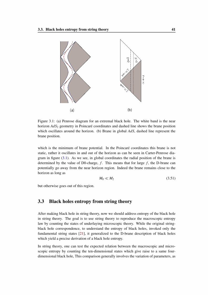
3.3. Black holes entropy from string theory 41

Figure 3.1: (a) Penrose diagram for an extremal black hole. The white band is the nearhorizon AdS2 geometry in Poincaré coordinates and dashed line shows the brane positionwhich oscillates around the horizon. (b) Brane in global AdS, dashed line represent thebrane position.

which is the minimum of brane potential. In the Poincaré coordinates this brane is notstatic, rather it oscillates in and out of the horizon as can be seen in Carter-Penrose dia-gram in figure (3.1). As we see, in global coordinates the radial position of the brane isdetermined by the value of D0-charge, f . This means that for large f , the D-brane canpotentially go away from the near horizon region. Indeed the brane remains close to thehorizon as long as

M0M2 (3.51)

but otherwise goes out of this region.

3.3 Black holes entropy from string theory

After making black hole in string theory, now we should address entropy of the black holein string theory. The goal is to use string theory to reproduce the macroscopic entropylaw by counting the states of underlaying microscopic theory. While the original string-black hole correspondence, to understand the entropy of black holes, invoked only thefundamental string states [21], it generalized to the D-brane description of black holeswhich yield a precise derivation of a black hole entropy.

In string theory, one can test the expected relation between the macroscopic and micro-scopic entropy by counting the ten-dimensional states which give raise to a same four-dimensional black hole, This comparison generally involves the variation of parameters, as


for the string coupling we have

Macroscopic regime: RH ls⇒ |Q|gs 1 (3.52)

Microscopic regime: |Q|gs 1 (3.53)

We see that for comparing the two regimes we have to go from the weak to strong couplingand it is not priori clear that whether the number of states are preserved under this interpo-lation. In the other word, in string theory computation of the entropy in microscopic levelcan be preformed in the limit when we neglect the effects of interactions, gs 1. Since ablack hole can only exist once the interactions are turned on. This means that exact com-putation of the entropy of a black hole in string theory requires that counting of the statesin weak coupling remains valid for all values of the coupling.As an example we compare the entropy of a Schwarzschild black hole with an extremalblack hole (c = h = 1)

S =A

4G=

4πM2G Schwarzchild

π(q2 + p2) Extremal(3.54)

The entropy of black hole is not independent of Newton constant, G, but interestingly, incase of the extremal black hole it is. The same applies to a supersymmetric black hole ingeneral N = 2 supergravity in four dimensions.To see what is the consequence of this property, we remind the relation between Newtonconstant and the string coupling constant which is given by G ∼ g2

s l2s , where gs and ls

denote the string coupling and the string length, respectively. So, since the entropy of asupersymmetric black holes is independent of gs, it is meaningful to compare the macro-scopic entropy with the microscopic description.This remarkable property is present in supersymmetric black holes. In other word, as longas supersymmetry is preserved, the results obtained in non-interacting regime are valid forany couplings. However, we note that when we compactify space-time, the supersymmetrypreserved if we curl up dimensions into cycles. To make black hole we wrap extended ob-jects around cycles where can cause breaking of supersymmetry too, so we consider specialconfigurations of wrapped objects which some supersymmetry survives.Moreover, there is a mechanism that ensures that the macroscopic entropy of a supersym-metric black hole is entirely specified in terms of the charges qI, pI

Smacro = Smacro(qI, pI) (3.55)

This is the attractor mechanism which first discovered for supersymmetric black holes[2, 22, 23] and later shown that it holds for extremal black hole even if not supersym-metric [24].

In the microscopic level, in D-brane picture, the large degeneracy which gives the sta-tistical interpretation to the thermodynamic entropy comes from all the possible internalexcitations of the wrapped branes which lead to a same four dimensional black hole in themacroscopic level. It has been shown [4, 25] that the entropy calculated using the D-brane

3.3. Black holes entropy from string theory 43

description agrees precisely with the classical Bekenstein-Hawking entropy. For a D4-D0Calabi-Yau black hole the problem of microscopically computing the entropy has also beensolved [26]. Specially, recently it was shown [7] that one can derive the entropy by doingcalculations in the proposed dual conformal field theory, CFT1. The CFT1 takes the formof quantum mechanics of a set of probe D0-branes moving in the AdS2 near-horizon ge-ometry. The non-abelian N-D0 configurations corresponding to D2 branes wrap the blackhole horizon and carry N units of world-volume magnetic flux. The D2-D0 brane is in thebackground magnetic flux on the CY3 and therefore acquires large degeneracy correspond-ing to the lowest Landau levels. Number of degeneracies found to be exactly reproduce theleading order area-entropy formula for a D4-D0 black hole.

In following we see how one can count the microscopic degeneracy of a black hole in stringtheory and we will see it precisely matches with the Bekenstein-Hawking entropy.

3.3.1 Example: D4-D0 black hole on T 6

To have a better view of the underlaying microscopic description and to see that if it agreeswith the macroscopic entropy we study the D4-D0 black hole which we considered earlier,namely, the configuration of three D4-branes with charges p1,p2,p3 and q0 D0-branes inIIA compactified on T 6. Macroscopic entropy can be calculated easily by looking at thearea of horizon. The horizon of the black hole is located in r = 0 and the area of the horizoncan be computed as

A = 4π limr→0

(r2

√q0 p1 p2 p3

r4

)= 4π

√q0 p1 p2 p3 (3.56)

In order to write down the Bekenstein-Hawking entropy it is instructive to restore dimen-sions. Specially, since the spectrum of charges are discrete one can introduce fundamentalcharge units c0, ci and express q0, p1, p2, p3 (which have length dimension) to be integersas

q0, pi ⇒ c0q0, ci pi (3.57)

With this description now we have p1 D4-branes wrapped on the y1,y2,y3,y4, p2 D4-braneswrapped on the y1,y2,y5,y6, p3 D4-branes wrapped on the y3,y4,y5,y6 and q0 D0-branes.One straightforward way is first to write down the entropy in terms of the masses via (3.21)

Smacro =A

4G4= 16πG4

√M0M1M2M3 (3.58)


Now we can use (3.35) and (3.36) as

M0 =1

gslsq0 (3.59)

M1 =1

gs(2π)4l5s(2πR1)(2πR2)(2πR3)(2πR4)p1

M2 =1

gs(2π)4l5s(2πR1)(2πR2)(2πR5)(2πR6)p2

M3 =1

gs(2π)4l5s(2πR3)(2πR4)(2πR5)(2πR6)p3

where R1, ...,R6 are the radii of the T 6 cycles. Furthermore we need to know the expresionfor four-dimensional Newton constants, G4

G4 =G10

VT 6, G10 = 8π

6g2s l8

s (3.60)

the resulting macroscopic entropy is

SBH = 2π

√q0 p1 p2 p3 (3.61)

All dimensionful constants and all continuous parameters cancel precisely and the entropyis a pure number which is given by the number of charges. Indeed, this indicates that aninterpretation in terms of the microscopic D-brane states is possible.The goal is to use the D-brane configuration to produce the entropy (3.61) by countingthe states, which originally performed in [27]. We should find, so to say, how this blackhole can be constructed in many possible ways. We count the states when there are nointeractions and the supersymmetry guarantees that the zero coupling counting holds fornonzero coupling, where we have a black hole.As we already mentioned, the microscopic entropy is the logarithm of states degeneracy,which leads to the same macroscopic quantities. In our case

Smicro = logN(q0, p1, p2, p3) (3.62)

where N(q0, p1, p2, p3) is the number of microstates of a black hole with macroscopic pa-rameters q0, p1, p2, p3. Lets start with an special case where we have only three D4-branes,p1 = p2 = p3 = 1. The three D4-branes intersect only at one point in T 6. Now we bindq0 D0-brane to the mutual intersection point by letting, massless, strings run between thezero-branes and each of the four-branes. To count the zero modes of the D0-brane in theintersection point, we note that two four-branes brake 3/4 of the original 32 supersym-metries, The third four-brane also breaks half of the remaining supersymmetry and hencewe are left with four bosonic modes. Furthermore, the unbroken supersymmetry impliesan equal number of fermionic degrees of freedom. The degeneracy of states, d(n), withcharge n is given by the coefficient of qn of generating function

∑n

d(n)qn =∞

∏k=1

(1+qk

1−qk

)4

(3.63)

3.4. Absorption of black holes in string theory 45

So, the degeneracy of states with three four-branes and q0 D0-charge, where q0 1, is

d(q0) = exp(2π√

q0) (3.64)

Returning to our example where p1, p2, p2 are greater than unity, we have three set of four-branes which each of them consists of many parallel four-branes. Separating four-branesgives p1 p2 p3 distinct points for the intersecting three four-branes. Binding q0 D0-brane toeach intersection points gives four bosonic and four fermionic modes, and hence total of4p1 p2 p3 bosonic/fermionic modes. The generating function of degeneracy is then

∑n

d(n)qn =∞

∏k=1

(1+qk

1−qk

)4p1 p2 p3

(3.65)

for large q0 is leads to degeneracy d(q0) = exp2π√

q0 p1 p2 p3 and the entropy is then

Smicro = 2π

√q0 p1 p2 p3 (3.66)

This coincides exactly with the Bekenstein-Hawking entropy (3.61) extracted from themetric. Our example can be generalized to Calabi-Yau black holes with arbitrary chargesq0, pA. This has been done in [26]. Without going to details we give the result

S = 2π

√|q0|(CABC pA pB pC + c2A pA) (3.67)

c2 is the second Chern class and CABC is the intersection number, which is fixed by thetopology of internal manifold. This holds both for the macroscopic and the microscopicdescription. Finally, returning to our example, since the torus T 6 is flat, the second Chernclass vanishes and the intersection form is CABC = εABC and A,B,C = 1,2,3 and hence weget same formula as before.

Apart from computing the statistical entropy of black holes, the D-brane method of blackholes can be also applied to derive the Hawking radiation and to compute the greybodyfactor. In what follows we mainly focus on the black hole absorption cross section inD-brane picture.

3.4 Absorption of black holes in string theory

We have made black holes in string theory and found that the microscopic physics of branesreproduces the Bekenstein entropy for near-extremal holes. A natural step beyond thecomparison of entropies is to interpret absorption cross sections for massless particles interms of the D-brane world-volume theories. In oder word, we can ask about the dynamicsof black holes: Can we compute the probability of the string state to absorb or emit quanta,and then compare this to the probability for the black hole to absorb infalling quanta oremit Hawking radiation?


In D-brane picture, absorption and Hawking radiation can be understood in terms of closedstrings. The absorption of massless scalars into black holes can be described in the effec-tive string language as a massless closed string state hitting a set of intersecting D-branesand turning into a pair of open strings that run in opposite directions along the 1 + 1-dimensional intersection manifold. Emission happens for near-extremal black holes, wherewe have, for example, sea of left movers and a right mover. Joining right mover with a leftmover form a massless closed string which leave the brane as Hawking radiation.

In order to calculate the absorption cross section in D-brane formalism one needs the lowenergy world-volume action for D-branes coupled to the massless bulk fields. These cou-plings may be deduces from the D-brane Born-Infeld action described earlier in this chap-ter.

3.5 Absorption on horizon-wrapped branes

Here we will be interested in the absorption cross section on such D2-branes as seen byan asymptotic observer. For this we need the coupling of the D2-branes to the space-timefields. This can be inferred from the Born-Infeld action

S =−µ2

∫d3

ξ e−Φ√−|G+2πα ′F |+µ2

∫Σ3

[P[C[3]]+2πα′F ∧P[C[1]]] , (3.68)

where Gab is the induced string frame world-volume metric for a given 10-dimensionalstring metric and C[1] is the RR 1-form in IIA theory with

dC[1] =R2

q0cosh χdτ ∧dχ . (3.69)

in global AdS2 coordinates. Fab is the field strength of the world-volume U(1) gauge po-tential, A with background value

A =− f2πα ′

cos(θ)dφ . (3.70)

Finally the background value of the dilaton is given by

eΦ0 =q0

R. (3.71)

3.5.1 Vibration modes

In what follows we will work in the static gauge and we will neglect internal excitationslevels in X which are suppressed in the approximation (3.13). In this case there is exactlyone transverse scalar field parameterizing the radial position of the brane in AdS2 as well a

3.5. Absorption on horizon-wrapped branes 47

gauge field Aa.There are two kind of fluctuations to be considered, one from radial position,δ χ , and other one is the fluctuations of gauge field living on the brane

χ → χ0 + εδ χ (3.72)

Fab → Fab + ε fab (3.73)

We take the D0-charge on the two-brane, q0 ∝∫

S2 F to be fixed. In this case the quantummechanical (s-wave) excitation δ χ decouples from all other excitations and can thus betreated separately. Upon substitution of the AdS2×S2 metric

ds2 = R2[−cosh2χdτ

2 +dχ2]+R2dΩ

22 (3.74)

in the Born-Infeld action and expanding up to second order in derivatives we find the actionfor the transverse scalar χ

SD2 =1g2

∫ [12

χ2−V1(χ)+V2(χ)

]dτ , (3.75)

with

V1(χ) =

√M2

2 +M20

M2cosh(χ) , V2(χ) =

M0

M2sinh(χ) , (3.76)

andg−2 = M2Re−Φ0 = 16πµ2D (3.77)

V1χ is sourced by DBI part of the action and V2(χ) originates from the Chern-Simons termin (3.68). Upon expanding the potential V to second order in δ χ we obtain a harmonicoscillator with frequency 1 (in units of 1/R) which can be quantized in standard way as

δ χ(τ) =g√2

(eiτa+ e−iτa†) , (3.78)

where a and a† are, respectively, the annihilation- and creation operators for the harmonicoscillator.

Next we consider quadratic fluctuations with non-vanishing angular momentum. By ex-panding the action (3.68) to second order in the fluctuation in the position δ χ and thegauge field, fab = ∂aAb−∂bAa, we obtain

S(2) =1g2

∫d3

ξ R3 sinθ12(δ χ)2 (3.79)

+1g2

∫d3

ξ R3 sinθ(gi j

∂iδ χ∂ jδ χ +(∂τδ χ)2) i, j = θ ,φ

− 1g2

∫d3

ξ R3 sinθ(2πα ′)2

f√

R4 + f 2Fab fabδ χ

+1g2

∫d3

ξ R3 sinθ(2πα ′)2

R4 + f 2

(1

sin2θ

f12 f12− f01 f01−1

sin2θ

f02 f02

)


Here S(2) refers to the action corresponding to second order fluctuations. We can simplifythe above action by introducing a modified metric as

gab = R2

−1 0 00 1 00 0 sin2(θ)

. (3.80)

action is then

S(2) =1

g24π

∫d3

ξ√−g[−1

2(δ χ)2− 1

2gab

∂aδ χ∂bδ χ− (3.81)

−14(2πα ′)2

R4 + f 2 gacgbd fab fcd +12

(2πα ′)2

f√

R4 + f 2Fab fabδ χ

],

Thus the dynamics of the quadratic fluctuations on a two-brane in AdS2 × S2 wrappedon S2 is identical to that of a brane fluctuating in R1,1× S2 with a non-trivial potentialV (δ χ, fab). The coupling between fab and χ persists in the absence of a D0 probe branecharge as a consequence of the Chern-Simons term in (3.68). The equations of motion forthe fluctuations obtained from (3.81) are then found to be

δS(2)

δAe= (2πα

′)2∇a

(f ae−

√R4 + f 2

fFae

δ χ

)= 0 , (3.82)

δS(2)

δ (δ χ)=

(∇

2−1)

δ χ +12

(2πα ′)2

f√

R4 + f 2Fab fab = 0 ,

where the indices are now lifted with g and ∇2 is with respect to g. To continue, using(3.82), we express fab in terms of a new scalar field, ψ , through

f ae =R2

(2πα ′)

1√g

εaeg

∂gψ +

√R4 + f 2

fFae

δ χ . (3.83)

Note that since we have defined ψ , via equation of motion this change of variables is validon-shell only. In terms of these new fields the equations of motion then take the form

∇2ψ−

√R4 + f 2

R2 ∂τδ χ = 0 , (3.84)

∇2δ χ +

R2√R4 + f 2

∂τψ = 0 .

In order to diagonalize this system we expand ψ and δ χ in spherical harmonics as

δ χ(τ,θ ,φ) = δ χlme−iΩτYlm(θ ,φ) (3.85)

δψ(τ,θ ,φ) = ψlme−iΩτYlm(θ ,φ)

Then the equation of motion leads to√R4+ f 2

R2

(−l(l +1)+Ω2

)−iΩ

iΩ R2√R4+ f 2

(−l(l +1)+Ω2

)(δ χlm

ψlm

)= 0 . (3.86)


Now we can derive the eigenfrequencies by finding the zero’s of the determinant. They aregiven by

Ω = l and Ω = l +1 (3.87)

with their corresponding eigenmodes

Φ0,1 =

1√2

(1

±i√

R4+ f 2

R2

)ϕ

0,1lm , (3.88)

respectively, where ϕ0,1lm are canonically normalized free fields with dispersion relation

Ω = l for ϕ0lm and Ω = l+1 for ϕ1

lm. We can thus quantize δ χ and ψ in terms of free fieldsalm and blm as(

δ χlm(τ)

ψlm(τ)

)=

g2

[alm√

leilτYlm

(1

−i√

R4+ f 2

R2

)+

a†lm√l

e−ilτY ∗lm

(1

i√

R4+ f 2

R2

)(3.89)

+blm√l +1

ei(l+1)τYlm

(1

i√

R4+ f 2

R2

)+

b†lm√

l +1e−i(l+1)τY ∗lm

(1

−i√

R4+ f 2

R2

)].

where we adopt the convention∫

S2 YlmY ∗l′m′ = 4πδll′δmm′ . The integer valuedness of thespectrum is to be expected since in global coordinates time τ ' τ +2π is compactified.

3.5.2 Absorption

The dilaton and the volume moduli of the CY (the latter is a fixed scalar) couple to theradial position χ of the two-branes in AdS2 as well as to the world-volume gauge potentialthrough the DBI-term in (3.68). The RR 1-form field couples to the world-volume gaugepotential and the radial position through the CS-term in (3.68). We will focus on the dila-ton absorption at present. To begin with we consider the quantum mechanical (s-wave)absorption of a dilaton δφ , which then couples to the transverse position as

SD2 =1g2

∫(−δφ)

(12

χ2−V1(χ)

)dτ . (3.90)

The potential V2 is induced by the CS-term in (3.68) and thus does not couple to the dilaton.To continue we need to distinguish between small- and large D0 probe-brane charge sinceδφ does not couple to V2. For M0 << M2 we have V1(χ0) ' 1 so that the back-reactionof the probe brane on the dilaton Φ can be neglected. For M2 << M0 on the other handV1(χ0) ∝

f 2

R4 >> 1 so that in the linearized approximation back reaction of the probe branedestabilizes the supergravity background7. We will thus not consider this possibility. Onthe other hand, for small D0 probe brane charge q0, the probe brane trajectory is within thenear horizon region of the Poincaré patch of AdS2. In this case it is interesting to computethe absorption cross section as observed by an asymptotic observer and compare it to theclassical black hole absorption cross section.

7Of course, in the full non-linear theory a (constant) deformation of the dilaton is a marginal deformationsince the position of the probe brane is a smooth function of the string coupling.


3.5.3 Spherical excitations without D0-charge

We will be interested in the absorption cross section seen by an observer static in AdS2 withrespect to Poincaré time8. We first consider the case of a probe brane without D0-charge,M0 = 0. In the near horizon AdS2 the classical solutions for an s-wave dilaton perturbationwith frequency ω with respect to the Poincaré time are given by

δφω(t) = eiω(t∓ R2r ) . (3.91)

3.5.3.1 Quantum mechanical mode

As a warm-up we first treat the absorption cross section in the harmonic oscillator ap-proximation (3.90), ie. assuming vanishing angular momentum of the excitations on theprobe-brane. In this case, by Taylor expansion the Lagrangian, the coupling of the dilatonperturbation to the transverse excitation of the two-brane is given by

Sint =1

2g2

∫δφ :

(− ˙δ χ

2+δ χ

2)

: , (3.92)

where " : : " denotes normal ordering and "˙" indicates derivative w.r.t. global time τ . Toleading order in g we get for an ingoing dilaton upon inserting (3.78)

〈2|Sint |0〉=√

22

3π

2∫− π

2

eiω(t− R2r )e−2iτdτ . (3.93)

Note that for M0 = 0, first order perturbation in δ χ vanishes and hence there is no transitionfrom the ground state to the first excited state |1〉. In order to evaluate the integral wechange to Kruskal coordinates which for χ0 = 0 are given by

vR = t− R2

r= R

sinτ−1cosτ

= R tan(τ− π

22

) , (3.94)

wR = t +R2

r= R

sinτ +1cosτ

= R tan(−τ + π

22

) .

Then

〈2|Sint |0〉 = −√

2∞+iε∫−∞+iε

11+ v2 eiωRv

(1− iv1+ iv

)2

dv (3.95)

= 2√

2πRω(Rω−1)e−Rω ,

where the contour C closes in the upper half plane for ω > 0 and passes above the poleat the origin in accordance with the iε prescription for absorption. The boundary term in(3.95) ensures the correct fall-off at v =±∞ required in order to recast this amplitude as a

8This time coincides with the time of an asymptotic observer in Minkowski space-time.


contour integral. Excitation to higher level is also possible and the corresponding amplitudecan be calculated by expanding V1 to higher order in χ . The corresponding amplitude issub-leading in g.

To determine the cross section for an s-wave dilaton into an s-wave excitation on the branefor an asymptotic observer in AdS2×S2 geometry we should compute the ingoing flux ofthe field φ , given in (3.91). By recalling the definition of conserved flux

F = 4π12i√

ggrr (φ∂rφ −φ∂rφ

)(3.96)

and AdS2×S2 metric

ds2 =− r2

R2 dt2 +R2

r2 dr2 +R2dΩ22 (3.97)

the ingoing flux is thenFAdS2 = 4πω (3.98)

The AdS2 cross section for this process is thus given by

σAdS2 =|A0→2|2

TF. (3.99)

= Rω(Rω−1)2e−2ωR

Here T = 2πR is the time interval in global coordinates. Of course, this is only part of thecomplete absorption cross section for an s-wave dilaton, since we ignored higher angularmomentum excitation so far. Never the less this partial cross section allows us to discusssome qualitative features. First we note that in spite of the discreteness of the spectrumof the D2-brane Hamiltonian, the D2-brane can absorb arbitrarily small frequencies withrespect to Poincaré time. This is in agreement with the classical picture of black hole ab-sorption. On the other hand, the low frequency behavior of (3.99) differs from the classicals-wave absorption cross section, which is proportional to the square of transmission coeffi-cient T that has a universal form for small frequencies 9 [10], |T |2 ' (Rω)2. We will comeback to this point in the conclusions. We should emphasize that the details of the absorp-tion process described here are qualitatively different from the world-volume absorption inflat space. In flat space, the low energy behavior is dominated by goldstone bosons andpossible other massless fields whereas here no massless degrees of freedom are present.The fact that the cross section vanishes linearly for ω → 0 is due precisely to the absenceof massless degrees of freedom.

3.5.3.2 Higher partial waves

After computing the absorption cross section for simple case of vanishing angular exci-tations, now we include such possibility to have total cross section. Recalling that the

9We have shown this universality in previous chapter.


Chern-Simons term does not couple to δφ we get the following interaction including allangular momenta on S2:

Sint =1

2g24π

3π

2∫− π

2

∫S2

δφ(t)[ √−g(

gab∂aδ χ∂bδ χ− R4

R4 + f 2 gab∂aδψ∂bδψ

)+

+2R2√

R4 + f 2δ χ∂τψ

]dτ . (3.100)

which can be obtained easily by using (3.83) and inserting, ψ in action of second orderperturbations (3.81). Now we use (3.89) to have in interaction in terms of free fields, wethen end up with

Sint =14 ∑

l 6=0,m

3π

2∫− π

2

eiω(t− R2r )(−1)m

[1l

a†lma†

l−me−i2lτ + (3.101)

+1√

l(l +1)a†

lmb†l−me−i(2l+1)τ +

1(l +1)

b†lmb†

l−me−i2(l+1)τ

]dτ .

Here we have ignored terms that contain the annihilation operators alm and blm since wetake the initial state to be the ground state so that they do not contribute to the absorptionamplitude. Note that if we include the l = 0 mode for the last term then we indeed recoverthe quantum mechanical mode discussed before. The transition amplitudes for fixed l > 0and m in leading order, in g, are then found to be 10

〈a, l m;a, l −m|Sint |0〉 = cm(−1)m

l

3π

2∫− π

2

eiω(t− R2r )e−i2lτdτ (3.102)

= 2cm(−1)m

l

∞+iε∫−∞+iε

11+ v2 eiωRv

(1− iv1+ iv

)2l

dv

= 2πcm(−1)l+m+1

lM2l, 1

2(2Rω) ,

with cm = 1/2 for m 6= 0, cm =√

2/4 for m = 0 and 〈a, l m;a, l −m| denotes the final stateconsisting of two excitations of type a with angular momentum l and L3 =±m respectively.Furthermore

Mλ ,µ(z) =zµ+ 1

2

22µB(12 +µ +λ , 1

2 +µ−λ )

1∫−1

e12 zt(1+ t)µ−λ− 1

2 (1− t)µ+λ− 12 dt (3.103)

10At the end of the section we give the details of how to compute the integral


is the Whittaker function [28] and B(x,y) is the beta function. Similarly

〈b, lm;b, l −m|Sint |0〉 = cm(−1)m

l +1

3π

2∫− π

2

eiω(t− R2r )e−i2(l+1)τdτ

= 2πcm(−1)l+m

l +1M2l+2, 1

2(2Rω) , (3.104)

for two b-type excitations in the final state and

〈b, lm;a, l −m|Sint |0〉 = cm(−1)m√l(l +1)

3π

2∫− π

2

eiω(t− R2r )e−i(2l+1)τdτ

=12

πi(−1)l+m+1√

l(l +1)M2l+1, 1

2(2Rω) , (3.105)

for one a-type and one b-type excitation in the final state. In order to obtain the total crosssection for absorption of an s-wave dilaton on a two-brane without D0-charge we haveto sum the partial cross section over l and m. Note that taking into account the quantummechanical mode the sum over l starts from 1 for (3.102) and (3.105) and from 0 for(3.104). Furthermore m= 0, · · · , l for (3.102) and (3.104) due to symmetry under m→−m,and m = −l, · · · , l for (3.105). Putting all this together and dividing by the incoming flux,FA dS∈ , we end up with

σAdS2 =1

4Rω

∞

∑l=1

1l|M2l, 1

2(2Rω)|2 + 1

32Rω

∞

∑l=1

2l +1l(l +1)

|M2l+1, 12(2Rω)|2 .

(3.106)

While we are not aware of any closed expression for the above sum we can never the lessextract the low frequency behavior with the help of an integral approximation of the sumsin (3.106). First we give the result and then describe how we get to it.

σAdS2 ' −5 Rω(log(Rω)+ const) , ω → 0 . (3.107)

The total absorption cross section is thus non-analytic at ω = 0. The absorption cross sec-tion for space-time scalars with non-vanishing angular momentum can be obtained alongthe same lines. We indicate the modifications later in this chapter.In order to isolate the low frequency behavior of the cross section (3.106) we use a conver-gent expansion of the Whittaker function Mλ ,µ(z) in a series of Bessel functions given byBuchholz [29]. It reads

Mλ ,µ(z) = Γ(2µ +1)22µzµ+ 12

∞

∑n=0

p(2µ)n (z)

J2µ+n(2√

λ z)

(2√

λ z)2µ+n, (3.108)

where p(2µ)n (z) are the Buchholz polynomials.

Assume that f (l) is a function such that f (l) ' 1/l for l >> 1 and let now L >> 1 be an


integer. Then we have for z→ 0

1z

∞

∑l=1

f (l)|M2l, 12(z)|2 ' 1

z

L

∑l=1

f (l)|M2l, 12(z)|2 + 1

z

∞

∑l=L

1l|M2l, 1

2(z)|2 = (3.109)

= C(L)z+4z2∞

∑l=L

1zl ∑

m,np(1)n (z)p(1)m (z)

J1+n(2√

2lz)J1+m(2√

2lz)(2√

2lz)2+n+m,

where C(L) is a z-independent constant that depends logarithmically on L. To continue wenote that p(1)n (z) is bounded by zn with p(1)0 (z) = 1. Furthermore for z→ 0 we can replacethe sum over l by an integral so that

1z

∞

∑l=1

f (l)|M2l, 12(z)|2 'Cz+4z∑

m,nzn+m

∞∫8zL

dxx

J2µ+n(√

x)J2µ+m(√

x)(√

x)2+n+m . (3.110)

This integral is well defined and finite apart from a logarithmic divergence for x→ 0. TheL-dependence between the first and second line cancels and we are left with

1z

∞

∑l=1

f (l)|M2l, 12(z)|2 ' 4z(log(z)+ const + ..) . (3.111)

3.5.4 Spherical excitations with D0-charge

Let us now consider a D2-brane which is charged under the D0-branes are bounded to it,with 0 < M0 << M2. In this case the interaction term at leading order in g is linear and wehave absorption to the first excited state,|1〉. In particular, for the absorption of an s-wavedilaton perturbation

Sint =M0

M2g2

3π

2∫− π

2

δφ(t)cosh(χ0)δ χdτ , (3.112)

so that leading order absorption amplitude becomes

〈1|Sint |0〉 =M0 cosh(χ0)√

2gM2

3π

2∫− π

2

eiω(t− 1r )e−iτdτ . (3.113)

This integral can again be brought in closed form with a suitable transformation of vari-ables,

〈1|Sint |0〉=√

2M0 cosh(χ0)√

2gM2

∞+iε∫−∞+iε

eiωRv(

11+ iv

)2

dv , (3.114)

leading to

〈1|Sint |0〉 = −iM0 cosh(χ0)

gM22√

2πRωe−Rω (3.115)

' −if

gR2 2√

2πRωe−Rω ,


where we have assumed f/R2 << 1 (which is concluded from 0 < M0M2). Proceedingas above we then obtain the AdS cross section

σAdS2 =f 2

g2R4 Rωe−2ωR . (3.116)

3.5.5 Dilaton with arbitrary angular momentum

So far we have only considered the absorption of s-wave dilaton, but this can be generalizedto find the absorption cross-section of a dilaton with an arbitrary angular momentum on aprobe brane with or with-out D0-charge, f . We compute the absorption of such a dilationfor non-vanishing D0-charge case and also give a overall view of how to compute theabsorption for uncharged D2-brane.

3.5.5.1 With D0-charge

Concretely we take the dilaton perturbation of the four space-time dilaton with arbitraryangular momentum

δφ(t,θ ,ϕ) = Ylm(θ ,ϕ)eiω(t∓ R2r ) . (3.117)

For f 6= 0 the dilaton couples to the probe brane oscillation through the first order interac-tion

Sint =f

R2g24π

3π

2∫− π

2

∫S2

√−g δφ

[cosh(χ0)δ χ +

(2πα ′)2

2 f 2 sinh(χ0)Fab fab

]dτ

=f

g2R2π

3π

2∫− π

2

∫S2

√−g δφ(t,θ ,ϕ)

[2

√R4 + f 2

R2 δ χ +∂0ψ

]dτ . (3.118)

The leading order, non-vanishing components of the transition amplitude for absorption ofa dilaton with angular momentum l,m into an a-type excitation is thus given by

〈a; lm|Slmint |0〉 =

√R4 + f 2 f

2gR4√

l

3π

2∫− π

2

eiω(t− R2r )(2+ l)e−ilτdτ

' − f (2+ l)il

gR2√

lπMl, 1

2(2Rω) , (3.119)

where we have ignored terms of order f 2 and higher when going from the first to thesecond line. Indeed we have argued above that for charged probe branes the absorptioncannot be treated perturbatively unless f << R2. Similarly we get for absorption into anb-type excitation

〈b; lm|Slmint |0〉 = − f (1− l)il+1

gR2√

l +1πMl+1, 1

2(2Rω)+O( f 2) . (3.120)


Note that a naive application of (3.120) for l = 0 leads to a√

2 discrepancy with the earlierresult (3.113). This apparent contradiction is resolved by recalling that for l = 0 there is noa-mode so that there is an extra

√2 in the normalization of (3.89). Note also that for l = 1

the amplitude for absorption in to a b-type excitation vanishes.

The total cross section for the absorption of φam is the again obtained by adding the squaresof the a- and b-type amplitudes (without summing over m). This gives

σAdS2 =f 2

8gRωR4

[(2+ l)2

l|Ml, 1

2(2Rω)|2 + (1− l)2

(l +1)|Ml+1, 1

2(2Rω)|2

],

(3.121)

which vanishes linearly for small ω .

3.5.5.2 Without D0-charge

To find the absorption cross-section for a dilaton with arbitrary angular momentum forvanishing D0-charge, f = 0, we consider the dilaton perturbation of the form

δφ(t,θ ,ϕ) = YLM(θ ,ϕ)eiω(t∓ R2r ) . (3.122)

taking (3.100), since now we have set of three spherical harmonic functions, the orthogo-nality condition we have used to write down (3.101) does not apply here, hence we have tokeep summation over l1,m1, l2,m2 and for example a†

lma†l−m replaces by a†

l1m1a†

l2m2and so

on.The integral over sphere can be expressed by 3 j symbol as∫

S2

y∗m1l1y∗m2l2yLM = (−1)l1+l2−L+M

√(2l1 +1)(2l2 +1)(2L+1)

4π

×(

l1 l2 L0 0 0

)(l1 l2 Lm1 m2 −M

)which, in turn can be calculated as a finite sum by using the Racah f ormula [30](

l1 l2 Lm1 m2 −M

)= (−1)l1−l2+M

√∆(l1l2L) (3.123)

×√

(l1−m1)!(l1 +m1)!(l2−m2)!(l2 +m2)!(L−M)!(L+M)!×∑t

1f (t)

where ∆(l1l2L) is a triangle coefficient

∆(l1l2L) :=(l1 + l2−L)!(l2 +L− l1)!(L+ l1− l2)!

(1+ l1 + l2 +L)!(3.124)

and

f (t) := t!(L− l2 +m1 + t)!(L− l1−m2 + t)!(l1 + l2−L− t)!(l1−m1− t)!(l2 +m2− t)!(3.125)


note that sum goes over all integer values of t for which the arguments of factorials arenon-negative.

3.5.6 Detailed calculation of absorption amplitude’s integral

For completeness we include the detailed calculation of the integrals appeared in (3.102)and (3.113). The integrals are in the form of

3π

2∫− π

2

dτeiω(t− R2r )e−iNτ (3.126)

where N is an arbitrary integer. We define variable x through

x := t− R2

r= R

cosh χ0 sinτ−1cosh χ0 cosτ + sinh χ0

, , (3.127)

Then we have3π

2∫− π

2

dτeiω(t− R2r )e−iNτ =

∮dxeiωRxe−iNτ(x) dτ

dx(3.128)

= 2A∮

dxeiωRx 11+ x2

(1− ix1+ ix

)N

= 2A2πiN!

(−i)N+1 [eiωRx(1− ix)N−1](N)

x=i ,

= (2π)

(i

1cosh χ0

− tanh χ0

)N N−1

∑k=0

(N−1

k

)(−2ω)N−k

(N− k)!e−ω .

where ”(N)“ denotes the number of derivatives and A is a constant

A =

(tanh χ0−

icosh χ0

)N

. (3.129)

This sum which appears in the result of integral is of the formN

∑k=0

(Nk

)1

(N +1− k)!(−2ω)N+1−k , (3.130)

we can write the sum in terms of Hypergeometric function, ie.

· · · = (−2ω)N

∑k=0

N!(N− k)!(N +1− k)!k!

(−2ω)N−k (3.131)

= (−2ω)N

∑p=0

N!(p)!(p+1)!(N− p)!

(−2ω)p p := N− k

= (−2ω)N

∑p=0

(−N)p

(2)p

(2ω)p

p!

= (−2ω)M(−N,2;2ω) =−eωM1+N, 12(2ω) ,


where M(a,b, ;z) is Confluent Hypergeometric function which is related to Whittaker func-tion, Mλ ,µ(z), by [28]

Mλ ,µ(z) = zµ+ 12 e−z/2M

(µ−λ +

12,2µ +1;z

)(3.132)

Therefore (3.126) has a solution as

3π

2∫− π

2

dτeiω(t− 1r )e−iNτ =−(2π)

(i

1cosh χ0

− tanh χ0

)N

MN, 12(2ω) . (3.133)

3.6 Discussion

In this chapter we reviewed the Calabi-Yau black holes arise in IIA string theory and par-ticularly we concerned with the special case of D4-D0 black hole. Afterward, by lookingat the entropy, we explained why we are interested in the supersymmetric black holes andhow they provide us the capability of identifying and counting the microstates of black holeand examining its equality to the macroscopic entropy.

As the main point, we have obtained analytic expressions for the low energy absorptioncross-section of space-time scalars on the horizon wrapped D2-branes, static in global co-ordinates of the near horizon AdS2 geometry. The fact that these amplitudes can be com-puted exactly may come as a surprise since the probe two-brane describes a complicatedtrajectory in the asymptotic Poincaré coordinates.

An interesting feature is that although the Hamiltonian of the D2-brane has a discrete spec-trum with spacing given by the inverse of the radius of the horizon the D2-brane can absorbarbitrarily small frequencies with respect to an asymptotic observer. We should mentionthat we only considered the bosonic sector of the world-volume theory. However, it isnot hard to see that fermions give a vanishing contribution at the lowest (quadratic) level.Also we have not considered fixed scalars in this paper although their inclusion should bestraight forward. As mentioned before, the details of the absorption process described hereare qualitatively different from the world-volume absorption on D-branes in flat space. Inflat space, the low energy behavior is dominated by goldstone bosons and possible othermassless fields whereas here no massless degrees of freedom are present. The fact thatthe cross section vanishes linearly for ω → 0 is due precisely to the absence of masslessdegrees of freedom.

In view of a possible interpretation for a dual interpretation of 4-dimensional CY-blackholes in terms of the quantum mechanics of probe D2-branes wrapped on the S2 of theirnear horizon geometry an encouraging result would have been to find agreement for the lowenergy absorption cross section on both sides. Our concrete calculation shows however thatthis is not the case since the microscopic absorption cross section on the two-brane doesnot have the correct behavior at small frequencies compared to the classical absorption

3.6. Discussion 59

cross section of massless scalars which vanishes quadratically in ω . However, the compar-ison between these two calculations is more subtle. First we note that our absorption crosssection was computed for wrapped D2-branes with small D0-charge whereas the dominantcontribution to the entropy comes from wrapped branes with large D0-charge. It wouldbe desirable to know the result in that case although the calculation appears to be moreinvolved since, as we showed, linearized perturbation theory breaks down in this situation.A possible application of the present calculation is to interpret a single wrapped D2-branewith small D0-charge as a small non-extremal perturbation of the extremal black hole. Thisis sensible since for small D0-charge the two-brane is confined to the near horizon AdS2

geometry of the asymptotically flat global geometry. In this case we should compare theclassical absorption cross section for the near extremal black hole with the the product ofthe transmission coefficient from asymptotically flat space to the near horizon AdS2 regionand the AdS2 absorption cross section computed in this paper. The microscopic cross sec-tion obtained in this way vanishes like (Rω)3. So we still have disagreement. One possibleexplanation for the disagreement could be that there are microscopic configurations, otherthan the wrapped D2-branes considered here, correspond to a non-extremal black holewhich reproduce the correct low energy behavior. One such generalization is to considermulti-branes wrapping horizon, however this does not change qualitative small frequencybehavior. Another possibility is to consider the scattering of massless space-time scalers onindividual probe D0-branes. However in that case the brane absorption amplitude vanishesdue to energy-momentum conservation.

CHAPTER 4

Supersymmetric Branes inCalabi-Yau Black hole

4.1 Introduction

In previous chapter, we saw that the extremal black holes in string theory play an importantrole to understand the precise microscopic description of four dimensional black holes ob-tained by the compactification of type IIA string theory on Calabi-Yau three-fold X . There,we restricted ourselves to the case where only the D4-D0 charges were non-zero on thebackground geometry. In general, we would like to get a precise microscopic descriptionof a four dimensional black hole with all possible charges of IIA theory, namely D6-D4-D2-D0 charges, all non-vanishing.

This is actually an outstanding problem in studying the extremal black holes in string theoryand their relation to the conformal field theories to get a precise microscopic description offour-dimensional black holes with D6-D4-D2-D0-charges obtained by the compactificationof type IIA string theory on a Calabi-Yau three-fold X . The charges are due to the D-branescompletely wrapped on the non-trivial cycles of X . For generic charges one expects thatthis black hole geometry to be dual to some conformal quantum mechanics on the boundaryof the near horizon AdS2 geometry.

For vanishing D6-charge the geometric entropy of such black holes can be given a micro-scopic understanding upon lifting this solution to M-theory. From the M-theory perspectivethis class of black holes are obtained by wrapping M5-branes with fluxes and momentumalong the M-theory circle and on a four-cycle in X . The corresponding near-horizon ge-ometry is dual to some 1+1-dimensional conformal field theory which lives on the dimen-sionally reduced five-brane world-volume [26]. This observation allowed the authors of[26] to derive the asymptotic degeneracy of states using standard methods of conformalfield theory. Upon compactification to IIA theory the near horizon geometry obtained isAdS2×S2. For this model a candidate for a dual quantum mechanics for the D4-D0 blackhole has been proposed [7] in terms of the degrees of freedom of probe D0-branes in thisbackground (see also [31, 32] for related discussions).

When the D6-brane charge is non-zero, the 4D black hole in IIA compactified on theCalabi-Yau may be lifted to a 5D black hole in M-theory on CY3×T Np0 , where T N de-notes the four-dimensional Euclidean Taub-NUT space with charges p0. While for largedistances compared to the size of the asymptotic Taub-NUT circle these black hole geome-

62 Chapter 4. Supersymmetric Branes in Calabi-Yau Black hole

tries asymptotes to R3× S1, and therefore are effectively four-dimensional, the M-theorycircle near the horizon is proportional to the size of the horizon so that the M-theory per-spective is more appropriate. Essentially, the near horizon geometry is a five-dimensionalspinning black hole sitting at the center of the Taub-NUT geometry, where the black holeis assumed to sit. This 4D-5D connection has been exploited in [33] to relate a certainpartition function of a class of four-dimensional black holes to that of five-dimensionalblack holes. The near horizon-geometry in five dimensions is essentially AdS2× S3/Zp0 .Consequently for non-vanishing D6-charge the problem is not directly related to a 1+1-dimensional CFT 1.

On the other hand it appears that the supersymmetric probe branes in the near horizongeometry play a role in understanding the dual quantum mechanics and the black holepartition function. They can be thought of as the “constituents” of the black hole in ques-tion. The asymptotic degeneracy of the electric constituents in the background flux geom-etry supported by the magnetic charges accounts for the black hole entropy in some cases[7, 32]. For instance it has been shown in [7] that the ground state degeneracy of D0-branesin a D4-brane flux background reproduces the correct asymptotic degeneracy for D4-D0charge black holes. Here the relevant Hamiltonian is the one of conformal quantum me-chanics on the moduli space of D0-branes in the flux background. An important subtlety isthough that the appropriate Hamiltonian appears to be that which generates translation in“global” time rather than Poincaré time which coincides with asymptotic time2. The dom-inant contribution to the entropy comes from D0-branes bound to two-branes wrapping thehorizon of the black hole.

On another front it has been shown [37] that the elliptic genus of the (0,4)-CFT [26] dual toblack holes with D4-D2-D0-charge has a dilute gas expansion dominated by multi-particlechiral primaries which are just the stationary M2 (and anti-M2) branes in global AdS3-coordinates, wrapped on holomorphic curves in the Calabi-Yau and sitting at the centerof AdS3. This provides a derivation of the OSV-conjecture relating the mixed partitionfunction of the black hole to the square of the topological string partition function [38].

In what follows we prepare the ground for extending the above-mentioned results [7, 37]to black holes with D6-charge by describing the supersymmetric probe branes in D6-charge backgrounds [9]. Of course, in this case we do not have a known “parent” 1+ 1-dimensional CFT to compare the probe-brane degeneracies with. Nevertheless one canhope that understanding the degeneracies of these states will give some insight aboutthe underlying microscopic theory. In Section 2 we will describe the eleven-dimensionalnear horizon geometry of a 4D black hole with generic D6-D4-D2-D0 charge. While thefull space-time geometry of a generic black hole with D6-charge is a solution of five-dimensional N = 2 supergravity with nv− 1 vector-multiplets, the attractor mechanism

1In fact it has been argued in [34] that black holes with D6-charge are related through a chain of stringdualities to BPS states without D6-charge. A similar relation was also conjectured in [35] based on an embed-ding of space-time in the total space of the U(1)-gauge bundle over near horizon geometry of the black hole.It would be interesting to see how these two approaches are related.

2The Poincare-Hamiltoinian has a continuos spectrum with no ground state as a consequence of the incom-pleteness of classical dynamics in Poincaré coordinates [36].

4.2. Supersymmetric properties of the branes 63

ensures that its near-horizon geometry is equivalently described in terms of N = 2 super-gravity with just one vector multiplet - the graviphoton, i.e. minimal supergravity in fivedimensions. A classification of the solutions of minimal supergravity in five dimensionscan be found in [39]. This property simplifies the task of finding the relevant Killing spinorsfor these black holes. In Section 3 we obtain the near horizon killing spinor in global co-ordinates and analyze the κ-symmetry for an stationary probe branes in global time alongthe lines of [20, 40]. In particular we find BPS two-branes wrapped on a holomorphictwo-cycle in the Calabi-Yau. These correspond to the zero-branes found in [40] and havethe right properties to be the relevant degrees of freedom for deriving the OSV-relationfor black holes with D6-charge. In addition we find BPS five-branes which wrap eithera holomorphic four-cycle in the Calabi-Yau and an S1 in space-time or wrap the horizonS3/Zp0 completely and a holomorphic two-cycle in the Calabi-Yau. These may play a roleanalogous to the horizon wrapped two-branes for D4-D0-black holes [7]. We plan to reporton these issues in subsequent work.

4.2 Supersymmetric properties of the branes

The world-volume action of D-branes have two symmetries. First, there is κ-symmetrywhich is a local symmetry and, second, global space-time supersymmetry which parametrizedby Killing spinors ε .

In general, a brane configuration trajectory will preserve the space-time supersymmetry ifthe action on the world-volume fermions can be compensated by the κ transformation. Inorder for the D-brane to be supersymmetric we only need to check that the κ-symmetrycondition

Γε = ε (4.1)

is satisfied. ε is the pull-back of Killing spinor on to the brane world-volume, correspond-ing to the unbroken supersymmetry and Γ is called the κ projection operator. The expres-sion for κ projection matrix, Γ, depends on the embedding map from the world-volume ofbrane into the space-time. For any Dp-brane, Γ is given by

Γ =

√deth√

det(G+F )∑n

12nn!

Γµ1ν1...µnνnFµ1ν1...µnνnΓ

n+ p−22

(11) Γ(0) (4.2)

Γ(0) =1

(p+1)!√

det hε

µ0...µpΓµ0...µp (4.3)

where the hatted indices are the world-volume coordinates and h is the determinant of thepull-back of the space-time metric to the world-volume, hab, and F = F +B. Killingspinors are the solution of Killing spinor equations, which are the equations of vanishingsupersymmetry transformations for the gravitino. The Killing spinor equation in eleven


dimensions is given by

0 =

[∇M +

1288

(Γ

N1N2N3N4M −8δ

N1M Γ

N2N3N4)

GN1N2N3N4

]ε11

∇M = ∂M +14

ωMABΓAB and G = dC[3] , (4.4)

where the capital indices run from zero to ten and ωMBA is the spin connection. Since we areinterested in black holes in lower dimensions, we would like to write the ten dimensionalspinor,ε11, as the tensor product of internal and non-compact spinors. In case of M-theory,this is to write the spinor as

ε11 = ε⊗η (4.5)

where, respectively, ε and η are the four dimensional and the internal (Calabi-Yau) spinors.The Killing equation on the Calabi-Yau is solved by the covariant constant spinors η±. Wehave chosen the following conventions: the γ-matrices on the X w.r.t. an orthonormal framewe denote by ρ i with

ρ i,ρ j= 2δij (4.6)

The spinors η± obey the relations

ρ(7)η± =±η± ,

ρiη+ = 0, ρiη− = 0 , (4.7)

where i and i are indices w.r.t. complex coordinates on X . The γ-matrices of five-dimensionalspace w.r.t. an orthonormal frame we denote by γa, such that the eleven-dimensionalγ-matrices ΓM, M = 0, ...,11, decompose the ΓM into a tensor product of five and six-dimensional γ-matrices,as

Γa = γ

a⊗ρ(7) , a = 0, ...,4 (4.8)

Γi = γ(5)⊗ρ

i = 1⊗ρi , i = 5, ...,11

where in the second line we have used that γ(5) = iγ01234 = 1. Decomposition of spinorsleads to the separation of Killing spinor equations and to treat their corresponding solutionsindependently. The five-dimensional space-time supersymmetry arises from the solutionsof Killing spinor equation are then[

∂M +14

ωMRPΓRP− i

4√

3

(FABΓ

ABM−4FMNΓ

N)]ε = 0 (4.9)

ε is a five-dimensional spinor. This leads to the five-dimensional equations and determinesthe Killing spinor ε . So the recipe for recognizing if a D-brane preserves some supersym-metry, is to find the Killing spinor and also determine the expression for Γ and see if theκ-symmetry condition (4.1) holds.

4.3. Supersymmetric branes in M-theory attractor geometries 65

4.3 Supersymmetric branes in M-theory attractor geometries

4.3.1 Near horizon geometry of D6-D4-D2-D0 black holes

In order to be self-contained and to fix the conventions we first review the relevant statichalf BPS solutions of four-dimensional N = 2 supergravity with nv vector multiplets [2].The general stationary BPS configurations were derived in [41, 42, 43]. We then describethe lift of these solutions to five dimensions [33] and determine the near horizon geometryfor a given set of four-dimensional charges.

We consider static single-centered BPS solutions in four dimensions. These solutions arecharacterized by their asymptotic magnetic and electric charges (pI,qI), I = 0, . . . ,nv andtheir asymptotic moduli. As such they are completely determined in terms of 2nv +2 realharmonic functions on R3

HI(r) = hI +pI

r, HI(r) = hI +

qI

r, (4.10)

subjected to the conditionpIhI−qIhI = 0 . (4.11)

The corresponding metric is given by

ds2(4) =−

π

S(r)dt2 +

S(r)π

d~x2 . (4.12)

The function S can be expressed as

S = 2π

√H0Q3− (H0L)2 , (4.13)

with

L =H0

2+

HAHA

2H0 +CABCHAHBHC

6(H0)2 ,

Q3/2 =16

CABCyAyByC . (4.14)

Here A,B,C ∈ 1, . . . ,nv and yA are implicitly determined by the equation

CABCyByC = 2HA +CABCHBHC

H0 . (4.15)

The gauge potentials are determined again by the harmonic functions (4.10) and S(r) (4.13)

AI(4) =

1S

∂S∂HI

dt +A I , dA I = ∗3dHI . (4.16)

To complete the four-dimensional description of generic D6-D4-D2-D0 attractor blackholes we give the complex scalar fields

tA =HA + i

π

∂S∂HA

H0 + iπ

∂S∂H0

. (4.17)


As mentioned above for generic values of these charges the string coupling becomes largein the near horizon regime. To allow for a unified description for generic charges we nowgive the lift of these solutions to five dimensions. For a nice discussion of this lift see forexample [44].

The five dimensional metric is given by

ds2(5) = 22/3V 2(dψ +A0

(4))2 +2−1/3V −1ds2

(4) (4.18)

= −(22/3Q)−2(dt +2L(dψ +A 0))2 +(22/3Q)(1

H0 (dψ +A 0)2 +H0d~x2) ,

with

V =

(16

CABCℑtAℑtB

ℑtC)1/3

=S

2πH0Q. (4.19)

The four and five dimensional gauge potentials are related by

AA(5) = ℜtA(dψ +A0

(4))−AA(4)

= −Y A

2Qdt +

(HA

H0 −LQ

Y A)(dψ +A 0)−A A (4.20)

where we introduced the five dimensional scalars

Y A =yA

Q1/2 . (4.21)

They obey the relation

16

CABCY AY BYC = 1 . (4.22)

Let us now take the near horizon limit, r pI,qI, of the five-dimensional solution. Forthis we define

σ =1r,

dΩ23 = dθ

2 + sin2θdφ

2 +(dψ/p0 + cosθdφ)2 ,

R2AdS = lim

r→0

(22/3H0Q

), (4.23)

J = limr→0

((H0)1/2L

Q3/2

)and

Y A0 = lim

r→0Y A .

Then, rescaling t appropriately (denoted again by t) we obtain [45]

ds2(5) = R2

AdS

(−(

dtσ

+ J(dψ/p0 + cosθdφ)

)2

+dσ2

σ2 +dΩ23

), (4.24)

AA(5) = −

Y A0 22/3√

3A+

pA

p0 dψ , (4.25)

A =

√3

2RAdS

(dtσ

+ J(dψ/p0 + cosθdφ)

). (4.26)


The near horizon geometry depends on three parameters: the D6 charge p0, the AdS2

radius RAdS which is determined by the value of Q at the horizon and the five-dimensionalangular momentum J. These are also the quantities that appear in the Bekenstein-Hawkingentropy. In other words, as pointed out in [33] (see also [46]) the Taub-NUT fibration,which interpolates between the four-dimensional and the five-dimensional geometry givesa simple geometric representation of the entropy formula for the 4D-entropy of D6-D4-D2-D0 black holes based on special geometry [47]. For J → 1 a closed light-like curvedevelops. This singular limit has recently been analyzed in [35].

4.3.2 Global coordinates and half BPS-branes, five-dimensional analysis

Next we introduce global coordinates. For this we start with the expressions (4.24) and(4.26) for the metric and gauge field respectively and change coordinates as (sinB := J)

t =cosBcosh χ sinτ

cosh χ cosτ + sinh χ,

RAdS σ =1

cosh χ cosτ + sinh χ, (4.27)

ψpoinc = ψ +2tanB tanh−1(e−χ tan(

τ

2)) .

The metric and field strength of the graviphoton then take the form

ds2(5) = R2

AdS(−cosh2

χdτ2 +dχ

2 +(sinBsinh χdτ− cosBσ3)2 +dΩ

22),

F =

√3

2RAdS (cosBcosh χdχ ∧dτ− sinBsinθdθ ∧dφ) , (4.28)

where dΩ22 is the line element of the unit two-sphere and

σ3 = dψ/p0 + cosθdφ .

It is straightforward to lift this near horizon geometry to eleven dimensions. The liftedgeometry is a direct product of the five-dimensional space and a Calabi-Yau three-fold Xwith Kähler form Y A

0 ωA where ωA ∈ H2(X ,Z) is a basis. The three-form C[3] in elevendimensions is proportional to the wedge product of the gauge field (4.26) with the Kählerform. Now to derive the Killing spinors from equations (4.9) we need first to have thefünf-beine and the spin connections. With a convenient choice of the fünf-beine

e0 = cosh χdτ, e1 = dχ ,

e2 = dθ , e3 = sinθdφ , (4.29)

e4 = cosB(

dψ

p0 + cosθdφ

)− sinBsinh χdτ ,


The spin connections are then given by

ω34 = −12

cosBe2, ω24 =12

cosBe3

ω14 =12

sinBe0, ω04 =−12

sinBe1

ω23 = −cosθ

sinθe3 +

12

cosBe4 (4.30)

ω01 = − sinh χ

cosh χe0− 1

2sinBe4

ω12 = ω02 = ω13 = ω03 = 0

Now, to solve the Killing equation we substitute (4.30) and (4.28) in the Killing spinorequation 4.4. The five-dimensional part of the Killing equation becomes

0 = ∂ψε ,

0 =

(∂φ +

12

cosBsinθγ24− 1

2cosθγ

23 +i2

sinBsinθγ2)

ε ,

0 =

(∂θ −

12

cosBγ34− i

2sinBγ

3)

ε , (4.31)

0 =

(∂τ +

12

sinBcosh χγ14− 1

2sinh χγ

01− i2

cosh χ cosBγ1)

ε ,

0 =

(∂χ −

12

sinBγ04 +

i2

cosBγ0)

ε .

These equations are solved by (see also [40])

ε = S(B,χ,τ,θ ,φ)ε0 ,

S(B,χ,τ,θ ,φ) = e−i2 Bγ4

e−i2 χγ0

ei2 τγ1

e12 θγ34

e12 φγ23

(4.32)

and ε0 is an arbitrary, constant four-component spinor.

We find the BPS configurations of M-branes that are wrapped on compact portions ofour background and, possibly, also (in case of M5-brane) have components tangent to thehorizon, and are point-like in the AdS space. In the following we classify the stationarysupersymmetric probe branes in this background.

This implies in particular that they are static in AdS2, i.e. χ = 0 but allows for M2-branesorbiting around the three-dimensional horizon as well as M5-branes partially or fully wrap-ping the horizon.

4.3.3 Half BPS M2-branes in global coordinates

We begin with the set of stationary, supersymmetric M2-branes wrapping a holomorphictwo-cycle in X . The κ-symmetry condition is [18]

Γ ε⊗η = ε⊗η (4.33)


with

Γ =1

(p+1)!√

dethε

abcΓabc

=1√h00

dX µ

dτea

µγa⊗ i1 , (4.34)

where we have assumed that the M2-brane has positive orientation. The hatted indicesare the world-volume coordinates and hab is the pull-back of the space-time metric to theworld-volume. The second line is expressed in static gauge X0 = 1. Having the form ofKilling spinor form (4.32) and plug it in the κ-symmetry condition (4.33) the BPS conditionis then

S−1ΓS ε0⊗η = ε0⊗η (4.35)

We need to know the component of S−1ΓS which are of the form S−1eabγaS for different

values of b. The explicit prefactors are3

S−1 ea0 γa S = cosBcosh χ cosτγ0 + isinBcosθγ

04 + icosBcosh χ sinτγ10

−isinBsinθ(cosφγ03− sinφγ

02)

S−1 ea1 γa S = cosBcosh χγ1 + sinBsinτ sinθ(cosφγ3− sinφγ2)− sinBsinτ cosθγ4

+cosBsinh χ sinτγ0− isinBcosτ cosθγ14− icosBsinh χ cosτγ

10

+isinBcosτ sinθ(cosφγ13− sinφγ

12)

S−1 ea2 γa S = cosBcosh χ cosτ(cosφγ2 + sinφγ3)− isinBsinθγ

32

+icosBsinh χ(cosφγ02 + sinφγ

03)+ isinBcosθ(cosφγ42 + sinφγ

43)

−icosBcosh χ sinτ(cosφγ12 + sinφγ

13)

(4.36)

S−1 ea3 γa S = cosBcosh χ cosτγ4− icosBcosh χ sinτγ

14 + icosBsinh χγ04

+isinBsinθ(cosφγ43− sinφγ

42)

S−1 ea4 γa S =

cosBp0cosh χ cosτ cosθγ4− cosh χ cosτ sinθ(cosφγ3− sinφγ2)

−icosh χ sinτ cosθγ14 + icosh χ sinτ sinθ(cosφγ

13− sinφγ12)

+isinh χ cosθγ04− isinh χ sinθ(cosφγ

03− sinφγ02)

Let us first consider the case where the two-brane sits at fixed θ and B but rotates in theφ direction. For φ 6= ±1 the BPS condition can never be satisfied. For φ = 1 we have√|h00|= |cos(B)sinh(χ)+ sin(B)cos(θ)| and

Γ(0) :=dX µ

dτea

µγa = −cosh χγ0 + sinθγ

3− sinBsinh χγ4 + cosBcosθγ

4 (4.37)

3In Appendix B we provide the a list of γ-matrix identities which are useful for computing the prefactorsof κ-symmetry condition


and

S−1Γ(0)S = cosBcosh χ cosτ(−γ

0 + γ4)+ i(cosBsinh χ + sinBcosθ)γ04

+icosBcosh χ sinτ(γ10− γ14)− isinBsinθ(cosφγ

03− sinφγ02)

+isinBsinθ(cosφγ43− sinφγ

42) . (4.38)

Requiring the κ-symmetry condition be independent of τ implies

γ04

ε0 =−ε0 . (4.39)

Furthermore if the latter condition is fulfilled we have

Γε⊗η =

(iΓ(0)√

h00ε

)⊗η = ε⊗η (4.40)

which is just the BPS condition (4.33). These solutions correspond to the zero branes foundin [40]. Note that this brane is BPS for φ = 1 while sitting at the north pole θ = 0 on thebase S2. This does not mean that this brane is static. Indeed, as the velocity along the fiberis given by ψ/p0+cosθφ , this configuration is geometrically equivalent to that with φ = 0and ψ = p0 which is a trajectory along the fiber of the S3/Zp0-bundle, i.e. a “great circle”on S3/Zp0 . If we assume instead that φ = const,θ = const, then ψ = p0 necessarily andthe BPS condition reads

[−cos(θ)γ04 + sin(θ)(cos(φ)γ03− sin(φ)γ02)]ε0 = ε0 . (4.41)

So the M2-brane can move along the fiber with constant velocity p0 and sits at any pointof the base space S2. The condition (4.41) reduces to (4.39) for θ = 0.

For ψ = 0, φ = φ0 (φ = φ0+π) constant and necessarily θ = 1 (θ =−1) the BPS conditionbecomes

(cos(φ)γ20 + sin(φ)γ30)ε0 = ε0. (4.42)

Geometrically, this is the case where the M2-brane moves along a meridian of the base S2

with constant velocity one and does not move along the fiber of the S3/Zp0-bundle over S2.

To summarize, an M2-brane on C2 is BPS if and only if it rotates with unit angular ve-locity on the covering space S3. For χ = 0 they describe uncharged null-geodesics on S3,while for χ > 0 the M2-branes are charged and follow a time-like trajectory 4. The ro-tation is required to stabilize them at fixed χ . This interpretation is compatible with thefour-dimensional analysis in [20] where it was observed that existence of static half-BPSbranes requires that the symplectic product of the charge vector of the probe brane with thebackground charges does not vanish. Let us consider rotation along the fiber first. Then,since the above results for the wrapped M2-branes are independent of B we can considervanishing B. In this case the non-vanishing of the symplectic product in four dimensions

4See [40] for a detailed analysis of the corresponding Born-Infeld action.


requires that the two-brane rotates along the fiber. Invoking rotational invariance on S3 wethen conclude that rotation along any geodesic circle of the S3 will lead to a half BPS-state.

Note also that a M2-brane sitting for example at θ = 0 and rotating in the fiber with ψ =

p0 preserves the same supersymmetry as an anti-M2-brane (i.e. negative orientation) atθ = π and ψ = p0. Thus these branes are mutually BPS. This property makes them naturalcandidates to extend the observation of [37] to black holes with D6-charge.

4.3.4 Half BPS five-branes

We now consider static M5-branes which partially, or fully wrap the horizon of the five-dimensional black hole. The remaining dimensions of the five-brane are wrapped on aholomorphic cycle in X .

4.3.4.1 M5 on C4×Y

For the M5-brane just to wrap the horizon partially, we wrap four dimensions of the braneon the four-cycle of X and the the rest dimension wrap each cycles of S3. We will assumethat the four-cycle C4 ∈ X is chosen such that the pull back of the RR-field dC[3] to theworld-volume of the five-brane vanishes. Then, since the coupling of the bulk to the world-volume three form F abc involves f ∗(dC[3]), we can consistently set F abc = 0. In additionwe will assume that the five-brane is wrapped holomorphically on C4. Then the CY-part ofΓ is just −1 [20], so that

Γ =1

(p+1)!√

dethε

abcde fΓabcde f

= − 12√

hε ab∂X µ∂Xν

∂σ a∂σ bea

µebνγab⊗1 . (4.43)

The generic situation can be understood by distinguishing three different S1-wrappings:

i) Y = (τ,θ): here√

h =

√cosh2(χ)− sin2(B)sinh2(χ) . (4.44)

We then conclude that the brane is BPS (Γε = ε) for χ = 0 provided

e−12 φγ23γ02e

12 φγ23ε0 =−ε0 . (4.45)

There is no condition on B and ψ . This brane wraps a geodesic circle in the horizon S3/Zp0

and is uncharged w.r.t. background fluxes.

ii) Y = (τ,φ): For B = 0 and χ = 0 the brane is BPS for all values of θ providedWe look at the case where χ = 0.


We have

Γ = − 12√

hετφ ∂X µ∂Xν

∂τ∂φea

µebνγab (4.46)

= − 12√

h(ea

τebφ − ea

φ ebτ)γab =−

12√

h(ea

0eb3− ea

3eb0)γab

= − 1√h(e0

0e33γ03 + e4

0e33γ43 + e0

0e43γ04)

= − 1√h(cosh χ sinθγ03− sinBsinh χ sinθγ43 + cosBcosh χ cosθγ04)

= −(sinθγ03 + cosBcosθγ04)

where in last line we imposed the restriction χ = 0. We need

S−1γ04S = −cosBcosθγ

04 + cosBsinθ(cosφγ03− sinφγ

02) (4.47)

−isinB(cosτγ0− isinτγ01)

S−1γ03S = −cosθ(cosφγ

03− sinφγ02)− sinθγ

04 (4.48)

So

S−1Γ(0)S = (sin2

θ + cos2 Bcos2θ)γ04 + icosBsinBcosθ(cosτγ0− isinτγ

01)

−(1− cos2 B)sinθ cosθ(cosφγ03− sinφγ

02) (4.49)

The BPS condition (for χ = 0) holds in two cases: First, for B = 0 the brane is BPS for allvalues of θ . In this case the brane wraps a geodesic in S3/Zp0 and is uncharged. Second,if B 6= 0 the brane is BPS only for θ = π

2 . Both cases provided

γ04ε0 =−ε0 . (4.50)

iii) Y = (τ,ψ): here the brane is BPS for χ = 0 and B = 0 provided

e−12 φγ23e−

12 θγ34γ04e

12 θγ34e

12 φγ23ε0 =−ε0. (4.51)

There is no solution for B 6= 0.

To summarize, a M5 on C4×Y is BPS provided it wraps a maximal geodesic circle inthe squashed horizon, S3/Zp0 . From the ten-dimensional perspective these results may beinterpreted as follows: An M5-brane wrapped along the S2 base becomes an NS5-brane inten-dimensions which is clearly uncharged and therefore static at χ = 0. If the M5-branesis wrapped along the S3-fiber instead, this will become a D4-brane with charge vectoraligned with that of the background. This brane cannot be static in global time unless thebackground flux vanishes, i.e. B = 0.

Note that the absence of static branes wrapped along the fiber for B 6= 0 does not excludestationary branes. Indeed for rotation in the φ direction, φ =±1, we have

Γ =−1√

h[cosh χ cosBγ04± sinθ cosBγ34] (4.52)


with√

det h =

√cos2 B(sinh2

χ + cos2 θ) . (4.53)

We need to have explicit form of S−1γ34S and S−1γ04S, they are as follows

S−1γ34S = cosB(cosφγ34− sinφγ42)− isinBcosh χ cosτ cosθ(cosφγ3− sinφγ2)

−isinBcosh χ cosτ sinθγ4− sinBcosh χ sinτ cosθ(cosφγ13− sinφγ12)

+sinBsinh χ cosθ(cosφγ03− sinφγ02)− sinBcosh χ sinτ sinθγ14

+sinBsinh χ sinθγ04 (4.54)

S−1γ04S = −cosBcosh χ cosθγ

04 + cosBcosh χ sinθ(cosφγ03− sinφγ

02)

−icosBsinh χ cosτ sinθ(cosφγ3− sinφγ2)+ cosBsinh χ sinτ cosθγ14

−cosBsinh χ sinτ sinθ(cosφγ13− sinφγ

12)− isinB(cosτγ0− isinτγ01)

+icosBsinh χ cosτ cosθγ4 (4.55)

So κ-symmetry condition derives as

[(−icos2 Bcosh χ sinh χ cosτ sinθ ∓ icosBsinBcosh χ cosτ sinθ cosθ)(cosφγ3− sinφ2)

+(−cos2 Bcosh χ sinh χ sinτ sinθ ∓ cosBsinBcosh χ sinτ cosθ sinθ)(cosφγ13− sinφ12)

+(cos2 Bcosh χ sinh χ cosθ ∓ cosBsinBcosh χ sin2θ)sinτγ

14

+(icos2 Bcosh χ sinh χ cosθ ∓ icosBsinBcosh χ sin2θ)cosτγ4

+cosBsinBcosh χ(sinτγ1 + icosτγ0)]ε0 = 0ε0 (4.56)

for τ-dependent terms, and

−1√cos2 B(sinh2

χ + cos2 θ)[(−cos2 Bcosh2

χ cosθ ± cosBsinBsinh χ sin2θ)γ04

+(cos2 Bcosh2χ sinθ ± cosBsinBsinh χ cosθ sinθ)(cosφγ

43− sinφγ42)

∓cos2 Bsinθ(cosφγ03− sinφγ

02)]ε0 = ε0 (4.57)

for τ-independent terms.The BPS condition is then given by

γ04

ε0 = ∓ε0 ,

sinh χ = ∓ tanBcosθ . (4.58)

It is clear that since χ = 0, for θ = π/2 the determinant vanishes and hence the brane cannot stay at the geodesic. These solutions correspond to rotating BPS configurations foundin [40].


4.3.4.2 M5 on C2×S3/Zp0

The induced metric hab is in this case−cosh2(χ)+ sin2(B)sinh2(χ) 0 −sin(B)sinh(χ)cos(B)cos(θ) − sin(B)sinh(χ)cos(B)

p0

0 1 0 0

−sin(B)sinh(χ)cos(B)cos(θ) 0 sin2(θ)+ cos2(θ)cos2(B) cos(θ)cos2(B)p0

− sin(B)sinh(χ)cos(B)p0 0 cos(θ)cos2(B)

p0cos2(B)(p0)2

and √

|h|= |cosh(χ)cos(B)sin(θ)/p0|. (4.59)

We will again assume that the brane is wrapped holomorphically on C2 so that the CY -partof Γ is 1⊗ iρ(7).

For B = 0 we then have

Γ =1

4!√

hε abcd∂X µ∂Xν∂Xρ∂Xδ

∂σ a∂σ b∂σ c∂σ dea

µebνec

ρedδ

Γabcd (1⊗ iρ(7)) (4.60)

= iγ0234⊗ρ(7)

so that the brane is BPS for χ = 0 and (iγ0234⊗ρ(7))(ε0⊗η) = ε0⊗η .

Next we consider the possibility of non-vanishing world-volume three-form flux F abc cor-responding to M2-branes wrapping C2 and bound to the M5-brane. For this we write

F =− f e2∧ e3∧ e4− f ∗6(e2∧ e3∧ e4) . (4.61)

Here f is proportional to the number of two-branes. Note that ea, a = 2,3,4 are the viel-beine on the unit three-sphere, not the three-sphere with radius RAdS on which the world-volume is wrapped and which determines the induced metric relevant for the ∗6 operation.Thus

∗6(e2∧ e3∧ e4) =1

R3AdS

e0∧ e5∧ e6 , (4.62)

where e0 is as in (4.30) and e5 and e6 are the zwei-beine on C2 with unit volume. SinceRAdS >> 1 we can neglect the last term in (4.61).

With this in mind we will now analyze the κ-symmetry condition. We find the representa-tion of [48] most convenient. Adapting the corresponding projector Γ to our situation weget

Γ =1√

1− 14 f 2

(1

6!√

dethε

abcde fΓabcde f −

12 ·3!

F abcγabc

)

=1√

1− 14 f 2

(iγ0234⊗ρ(7)+

12

f γ234

). (4.63)


To study the BPS condition Γε = ε we need to know that

S−1γ0234S = cosh χγ0234 + isinh χ(cosτγ234− isinτγ1234)

S−1γ234S = cosh χ(cosτγ234− isinτγ1234)− isinh χγ0234

then we can compute

S−1ΓS =

1√1− 1

4 f 2[−(cosτγ234− isinτγ1234)(sinh χ⊗ρ

(7)− 12

f cosh χ)

+i(cosh χ⊗ρ(7)− 1

2f sinh χ)γ0234]ε0 = ε0 (4.64)

The BPS condition then implies that

(sinh χ⊗ρ(7)− 1

2f cosh χ)ε0 = 0 (4.65)

i√1− 1

4 f 2(cosh χ⊗ρ

(7)− 12

f sinh χ)γ0234ε0 = ε0 (4.66)

Satisfying first line of above condition, we get

| f |= 2tanh(χ) (4.67)

For 12 f = ± tanh χ we conclude that ρ(7) must act on ε0 as ρ(7)ε0 = ±ε0 and the BPS

condition is iγ0234ε0 = ε0 and ρ(7)η = η for f > 0

iγ0234ε0 =−ε0 and ρ(7)η =−η for f < 0 .(4.68)

Upon double dimensional reduction along the fiber of S3/Zp0 to ten dimensions we get aD4-brane with

Fab = F4ab (4.69)

which in turn is SUSY according to [20].

Let us now analyze the case with non-vanishing four-brane flux B 6= 0. We make the Ansatz

F = ge0∧ e2∧ e3 . (4.70)

The the κ-symmetry projector

Γ =1√

1+ 14 g2

(iγ0234⊗ρ(7)−

12

gγ023

). (4.71)


calculating S−1γ0234S and S−1γ234S for this case, we get

S−1γ0234S = cosBcosh χγ0234 + icosBsinh χ(cosτγ423− isinτγ1423)

−isinBcosτ sinθ(cosφγ024 + sinφγ034)+ sinBsinτ cosθγ0312

+sinBsinτ sinθ(cosφγ0241 + sinφγ0341)− isinBcosτ cosθγ023 (4.72)

S−1γ023S = cosBcosτ cosθγ023 + cosBcosτ sinθ(cosφγ024 + sinφγ034)

+icosBsinτ cosθγ0312 + icosBsinτ sinθ(cosφγ0241 + sinφγ0341)

−isinBcosh χγ0234 + sinBsinh χ(cosτγ423− isinτγ1423) (4.73)

By imposing the κ-symmetry condition we have[isinτ sinθ(sinB⊗ρ

(7)− 12

gcosB)(cosφγ0241 + sinφγ0341)

+cosτ sinθ(sinB⊗ρ(7)− 1

2gcosB)(cosφγ024 + sinφγ034)

−(cosBsinh χ⊗ρ(7)+

12

gsinBsinh χ)(cosτγ423− isinτγ1423)

−isinτ cosθ(sinB⊗ρ(7)− 1

2gcosB)γ0312

+cosτ cosθ(cosB⊗ρ(7)− 1

2gcosB)γ023

]ε0 = 0 (4.74)

i√1+ 1

4 g2(cosBcosh χ⊗ρ

(7)+12

gsinBcosh χ)γ0234ε0 = ε0 (4.75)

(4.74) and (4.75) implies the BPS condition for χ = 0 andiγ0234ε0 = ε0 , ρ(7)η = η

12 g = tan(B) or

iγ0234ε0 =−ε0 ,ρ(7)η =−η12 g =− tan(B) .

(4.76)

For g 6= 0 these configurations describe M5-branes with delocalized M2-branes ending onthem.

If both, f and g are non-vanishing then the τ-dependent/independent terms of BPS condi-tion reads off the be [

isinτ sinθ(sinB⊗ρ(7)− 1


+cosτ sinθ(sinB⊗ρ(7)− 1


−(sinh χ cosB⊗ρ(7)+

12

gsinBsinh χ− 12

f cosh χ)(cosτγ423− isinτγ1423)

−isinτ cosθ(sinB⊗ρ(7)− 1

2gcosB)γ0312

+cosτ cosθ(sinB⊗ρ(7)− 1

2gcosB)γ023

]ε0 = 0 (4.77)

i√1+ 1

4 g2(cosBcosh χ⊗ρ

(7)+12

gsinBcosh χ− 12

f sinh χ)γ0234ε0 = ε0 (4.78)

4.4. Discussion 77

The κ-symmetry projector takes the form

Γ =1√

1+ 14(g

2− f 2)

(iγ0234⊗ρ(7)+

12( f γ234−gγ023)

). (4.79)

and the BPS-condition readsiγ0234ε0 = ε0 , ρ(7)η = η , 1

2 g = tan(B), 12 f = tanh(χ)

cosB , or

iγ0234ε0 =−ε0 , ρ(7)η =−η , 12 g =− tan(B), 1

2 f =− tanh(χ)cosB .

(4.80)

Thus, an static M5-brane wrapped on the horizon and a two-cycle in X with M2-branes onC2 bound to it is BPS for certain values of χ .

4.4 Discussion

I this chapter we constructed supersymmetric probe branes, stationary in global coordinatesof the eleven-dimensional near-horizon geometry, of a generic four-dimensional, single-centered attractor black hole. The motivation for this study came from the success of[7, 37] in approximating the black hole partition function by a dilute gas of non-interactingprobe branes in the near horizon geometry of attractor black holes without D6-charge. Ourresults should provide the necessary ingredients for extending this approach to includeD6-charge as well. In particular, we expect the M2-branes found here to be relevant for un-derstanding the OSV partition function in the presence of D6-charge. Similarly the horizonwrapping M5-branes should contribute, as collective excitations, to the partition functionof the conformal quantum-mechanical system dual to the AdS2 near horizon geometry.

CHAPTER 5

Discussion and Conclusion

In this thesis we studied the microscopic behavior of Calabi-Yau black holes in IIA stringtheory. First in chapter 2, we reviewed the classical black holes and their thermody-namical properties. We calculated the absorption cross-section of massless scalars onSchwarzschild and Reissner-Nordström black holes and also reviewed the universality oflow energy absorption cross-section. In chapter 3, by employing AdS/CFT correspon-dence, we obtained an analytic expressions for the low energy absorption cross-section ofa massless space-time scalars on the horizon-wrapped D2-branes, static in global coordi-nates of the near horizon AdS2 geometry of Calabi-Yau black hole. The fact that theseamplitudes can be computed exactly may come as a surprise since the probe two-branedescribes a complicated trajectory in the asymptotic Poincaré coordinates. For small butnon-zero probe D0-charge we found that the quantum mechanical absorption cross sectionseen by an asymptotic anti-deSitter observer, static in Poincaré time vanishes linearly in ω

for small frequencies. For vanishing probe D0-charge the absorption cross section has non-analytic (ω log(ω)) behavior. This is in disagreement with the classical s-wave absorptioncross section by the black hole which vanishes quadratically in ω for small frequencies.However, the comparison with the classical result is more subtle since for the classical ab-sorption cross section on near extremal black holes the potentials outside the near horizonAdS2 geometry is the only relevant one. This is because there is no reflection in AdS2.

An interesting feature is that although the Hamiltonian of the D2-brane has a discrete spec-trum with spacing given by the inverse of the radius of the horizon the D2-brane can absorbarbitrarily small frequencies with respect to an asymptotic observer. We should mentionthat we only considered the bosonic sector of the world-volume theory. However, it isnot hard to see that fermions give a vanishing contribution at the lowest (quadratic) level.Also we have not considered fixed scalars in this paper although their inclusion should bestraight forward. As mentioned before, the details of the absorption process described hereare qualitatively different from the world-volume absorption on D-branes in flat space. Inflat space, the low energy behavior is dominated by goldstone bosons and possible othermassless fields whereas here no massless degrees of freedom are present. The fact thatthe cross section vanishes linearly for ω → 0 is due precisely to the absence of masslessdegrees of freedom.

In view of a possible interpretation for a dual interpretation of four-dimensional CY blackholes in terms of the quantum mechanics of probe D2-branes wrapped on the S2 of theirnear horizon geometry an encouraging result would have been to find agreement for thelow energy absorption cross section on both sides. Our concrete calculation shows how-

80 Chapter 5. Discussion and Conclusion

ever that this is not the case since the microscopic absorption cross section on the two-branedoes not have the correct behavior at small frequencies compared to the classical absorp-tion cross section of massless scalars which vanishes quadratically in ω . However, thecomparison between these two calculations is more subtle. First we note that our absorp-tion cross section was computed for wrapped D2-branes with small D0-charge whereas thedominant contribution to the entropy comes from wrapped branes with large D0-charge.A possible application of the present calculation is to interpret a single wrapped D2-branewith small D0-charge as a small non-extremal perturbation of the extremal black hole. Thisis sensible since for small D0-charge the two-brane is confined to the near horizon AdS2

geometry of the asymptotically flat global geometry. In this case we should compare theclassical absorption cross section for the near extremal black hole with the the product ofthe transmission coefficient from asymptotically flat space to the near horizon AdS2 regionand the AdS2 absorption cross section computed in this paper. The microscopic cross sec-tion obtained in this way vanishes like (Rω)3. So we still have disagreement. One possibleexplanation for the disagreement could be that there are microscopic configurations, otherthan the wrapped D2-branes considered here, correspond to a non-extremal black holewhich reproduce the correct low energy behavior. One such generalization is to considermulti-branes wrapping horizon, however this does not change qualitative small frequencybehavior. Another possibility is to consider the scattering of massless space-time scalers onindividual probe D0-branes. However in that case the brane absorption amplitude vanishesdue to energy-momentum conservation.It would be desirable to know the result in that case although the calculation appears tobe more involved since, as we showed, linearized perturbation theory breaks down in thissituation.

In chapter 4, we constructed supersymmetric probe branes, stationary in global coordi-nates of the eleven-dimensional near-horizon geometry of a four-dimensional black holewith generic D6-D4-D2-D0-charges. The motivation for this study came from the success[7, 37] in approximating the black hole partition function by a dilute gas of non-interactingprobe branes in the near horizon geometry of attractor black holes without D6-charge. Inparticular we found BPS two-branes wrapped on a holomorphic two-cycle in the Calabi-Yau. Also, we determine the trajectories of the five-brane which preserve supersymmetryfor the case of wrapping a holomorphic four-cycle in the Calabi-Yau and an S1 in space-time (hence partially wrapping the horizon) and for the case of fully wrapped the horizonS3/Zp0 and a holomorphic two-cycle in the Calabi-Yau. Our results should provide thenecessary ingredients for extending this approach to include D6-charge as well. In particu-lar, we expect the M2-branes found here to be relevant for understanding the OSV partitionfunction in the presence of D6-charge. Similarly the horizon wrapping M5-branes shouldcontribute, as collective excitations, to the partition function of the conformal quantum-mechanical system dual to the AdS2 near horizon geometry.

APPENDIX A

Calabi-Yau spaces

Here we give a brief overview of essential concepts leading to the definition of the Calabi-Yau manifold, we follow mostly [49, 50, 51]. Calabi-Yau space is a manifold X withRiemannian metric g which satisfies following three conditions:

• X is complex manifold.This means that Calabi-Yau looks locally like Cn for some n, in the sense that it canbe covered by patches admitting local complex coordinates

z1, ...,zn (A.1)

and the transition functions between patches are holomorphic. Consequently, the realdimension of X is 2n, and hence Calabi-Yau spaces are even-dimensional manifolds,known as Calabi-Yau n-folds. Furthermore, the metric g should be Hermitian withrespect to the complex structure. This means

gi j = gi j = 0 (A.2)

so the only non-vanishing components of metric are gi j.

• X is Kähler.This means that there is a real function K locally on X such that

gi j = ∂i∂ j K (A.3)

where together with a Hermitian metric g one can define its associated kähler form

k = gi j dzi∧dz j (A.4)

The Kähler condition is then dk = 0.

• X admits a global holomorphic n-forms In each local coordinate patch of X one canwrite many such forms

Ω = f (z1, ...,zn)dz1∧ ...∧dzn (A.5)

where f is an arbitrary holomorphic function. For compact Calabi-Yau manifoldthere is at most on nowhere vanishing one such form, up to an overall scalar rescal-ing. Topologically this is equivalent to vanishing first Chern class.

82 Appendix A. Calabi-Yau spaces

So, briefly, a Calabi-Yau n-fold is a Kähler manifold having n complex dimensions andvanishing first Chern class.

Calabi-Yau manifold, defined above, has an important property: Metric on the Calabi-Yaumanifold is Ricci-flat

Ri j = 0 (A.6)

Compact Calabi-Yau manifold for n = 1 is torus T 2, for n = 2 just T 4 and K3, but forn = 3it is not even known whether the number of compact Calabi-Yau spaces is finite. T 6

is an example

A Calabi-Yau n-fold is characterized by the values of its Hodge numbers hp,q, which countthe number of harmonic (p,q)-forms on the manifold. These numbers do not characterizeCalabi-Yau manifold completely but specify a class of manifolds which have same Hodgenumbers. Hodge numbers satisfy following relations

hp,0 = hn−p,0

hp,q = hq,p (A.7)

hp,q = hn−q,n−p

First relation follows from the fact that the manifolds with de Rham cohomology H p(X)

and Hn−p(X) are isomorphic, second relation comes from complex conjugation and lastone is given by Poincaré duality. Furthermore, for any complex manifold h1,1=1. In addi-tion we have h1,0 = h0,1 = 0.There is also Betti number bp determines the dimension of H p(X), which counts the num-ber of lineally independent harmonic p-forms on the manifold

bk =k

∑p=0

hp,k−p(−1)pbp (A.8)

Therefore, in case of Calabi-Yau three-fold one requires only to specify h1,1 and h2,1. Fi-nally, the Euler characteristic of our manifold is just the alternating sum of Betti numbers:

χ(X) =2n

∑p=0

(A.9)

where for n = 3 gives χ = 2(h1,1−h2,1).

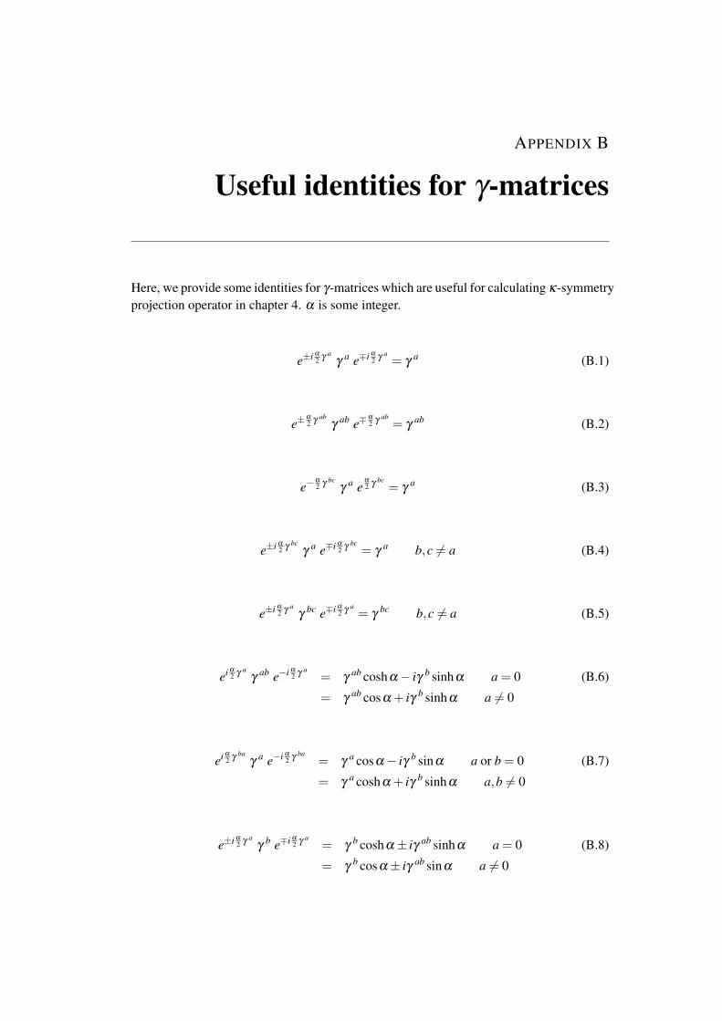
APPENDIX B

Useful identities for γ-matrices

Here, we provide some identities for γ-matrices which are useful for calculating κ-symmetryprojection operator in chapter 4. α is some integer.

e±i α

2 γ aγ

a e∓i α

2 γ a= γ

a (B.1)

e±α

2 γ abγ

ab e∓α

2 γ ab= γ

ab (B.2)

e−α

2 γ bcγ

a eα

2 γ bc= γ

a (B.3)

e±i α

2 γ bcγ

a e∓i α

2 γ bc= γ

a b,c 6= a (B.4)

e±i α

2 γ aγ

bc e∓i α

2 γ a= γ

bc b,c 6= a (B.5)

ei α

2 γ aγ

ab e−i α

2 γ a= γ

ab coshα− iγ b sinhα a = 0 (B.6)

= γab cosα + iγ b sinhα a 6= 0

ei α

2 γ baγ

a e−i α

2 γ ba= γ

a cosα− iγ b sinα a or b = 0 (B.7)

= γa coshα + iγ b sinhα a,b 6= 0

e±i α

2 γ aγ

b e∓i α

2 γ a= γ

b coshα± iγ ab sinhα a = 0 (B.8)

= γb cosα± iγ ab sinα a 6= 0

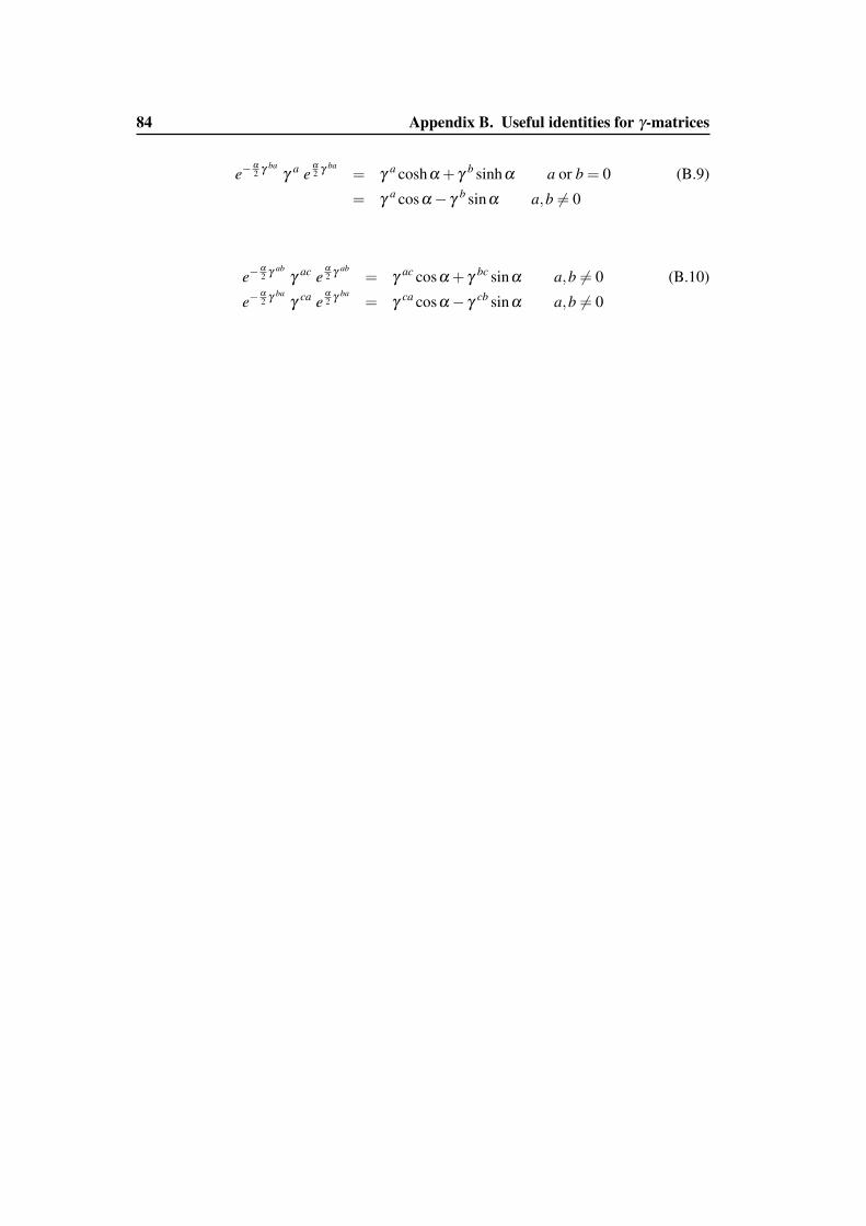
84 Appendix B. Useful identities for γ-matrices

e−α

2 γ baγ

a eα

2 γ ba= γ

a coshα + γb sinhα a or b = 0 (B.9)

= γa cosα− γ

b sinα a,b 6= 0

e−α

2 γ abγ

ac eα

2 γ ab= γ

ac cosα + γbc sinα a,b 6= 0 (B.10)

e−α

2 γ baγ

ca eα

2 γ ba= γ

ca cosα− γcb sinα a,b 6= 0

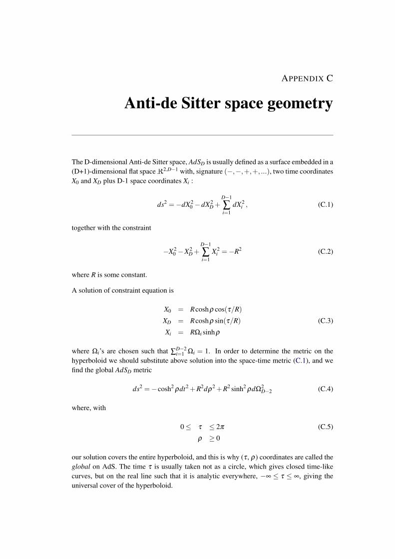
APPENDIX C

Anti-de Sitter space geometry

The D-dimensional Anti-de Sitter space, AdSD is usually defined as a surface embedded in a(D+1)-dimensional flat spaceR2,D−1 with, signature (−,−,+,+, ...), two time coordinatesX0 and XD plus D-1 space coordinates Xi :

ds2 =−dX20 −dX2

D +D−1

∑i=1

dX2i , (C.1)

together with the constraint

−X20 −X2

D +D−1

∑i=1

X2i =−R2 (C.2)

where R is some constant.

A solution of constraint equation is

X0 = Rcoshρ cos(τ/R)

XD = Rcoshρ sin(τ/R) (C.3)

Xi = RΩi sinhρ

where Ωi’s are chosen such that ∑D−2i=1 Ωi = 1. In order to determine the metric on the

hyperboloid we should substitute above solution into the space-time metric (C.1), and wefind the global AdSD metric

ds2 =−cosh2ρdt2 +R2dρ

2 +R2 sinh2ρdΩ

2D−2 (C.4)

where, with

0≤ τ ≤ 2π (C.5)

ρ ≥ 0

our solution covers the entire hyperboloid, and this is why (τ , ρ) coordinates are called theglobal on AdS. The time τ is usually taken not as a circle, which gives closed time-likecurves, but on the real line such that it is analytic everywhere, −∞ ≤ τ ≤ ∞, giving theuniversal cover of the hyperboloid.

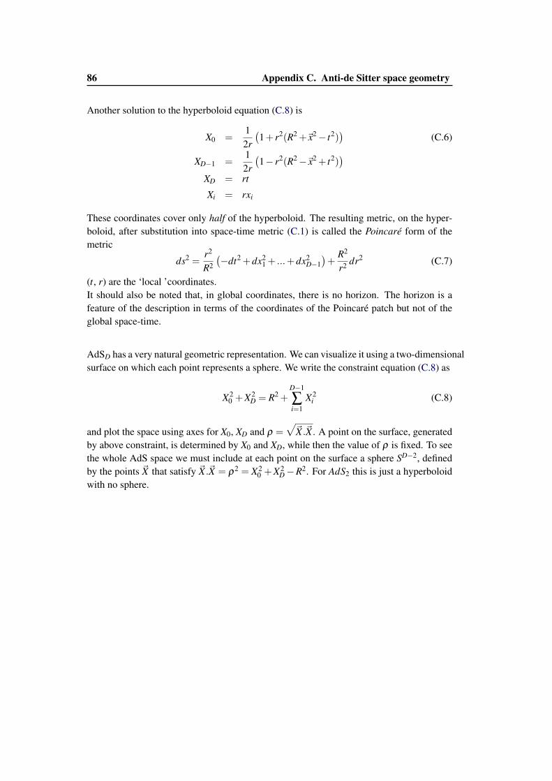
86 Appendix C. Anti-de Sitter space geometry

Another solution to the hyperboloid equation (C.8) is

X0 =12r

(1+ r2(R2 +~x2− t2)

)(C.6)

XD−1 =12r

(1− r2(R2−~x2 + t2)

)XD = rt

Xi = rxi

These coordinates cover only half of the hyperboloid. The resulting metric, on the hyper-boloid, after substitution into space-time metric (C.1) is called the Poincaré form of themetric

ds2 =r2

R2

(−dt2 +dx2

1 + ...+dx2D−1)+

R2

r2 dr2 (C.7)

(t, r) are the ‘local ’coordinates.It should also be noted that, in global coordinates, there is no horizon. The horizon is afeature of the description in terms of the coordinates of the Poincaré patch but not of theglobal space-time.

AdSD has a very natural geometric representation. We can visualize it using a two-dimensionalsurface on which each point represents a sphere. We write the constraint equation (C.8) as

X20 +X2

D = R2 +D−1

∑i=1

X2i (C.8)

and plot the space using axes for X0, XD and ρ =√~X .~X . A point on the surface, generated

by above constraint, is determined by X0 and XD, while then the value of ρ is fixed. To seethe whole AdS space we must include at each point on the surface a sphere SD−2, definedby the points ~X that satisfy ~X .~X = ρ2 = X2

0 +X2D−R2. For AdS2 this is just a hyperboloid

with no sphere.

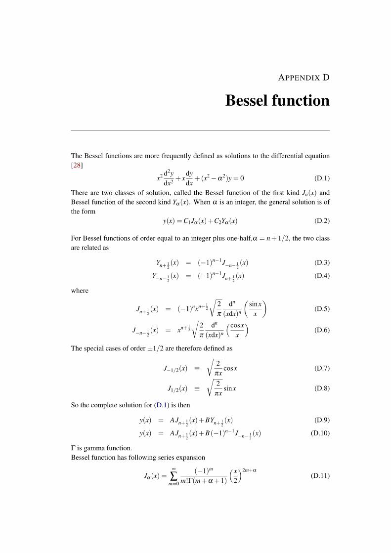
APPENDIX D

Bessel function

The Bessel functions are more frequently defined as solutions to the differential equation[28]

x2 d2ydx2 + x

dydx

+(x2−α2)y = 0 (D.1)

There are two classes of solution, called the Bessel function of the first kind Jn(x) andBessel function of the second kind Yα(x). When α is an integer, the general solution is ofthe form

y(x) =C1Jα(x)+C2Yα(x) (D.2)

For Bessel functions of order equal to an integer plus one-half,α = n+1/2, the two classare related as

Yn+ 12(x) = (−1)n−1J−n− 1

2(x) (D.3)

Y−n− 12(x) = (−1)n−1Jn+ 1

2(x) (D.4)

where

Jn+ 12(x) = (−1)nxn+ 1

2

√2π

dn

(xdx)n

(sinx

x

)(D.5)

J−n− 12(x) = xn+ 1

2

√2π

dn

(xdx)n

(cosxx

)(D.6)

The special cases of order ±1/2 are therefore defined as

J−1/2(x) ≡√

2πx

cosx (D.7)

J1/2(x) ≡√

2πx

sinx (D.8)

So the complete solution for (D.1) is then

y(x) = AJn+ 12(x)+BYn+ 1

2(x) (D.9)

y(x) = AJn+ 12(x)+B(−1)n−1J−n− 1

2(x) (D.10)

Γ is gamma function.Bessel function has following series expansion

Jα(x) =∞

∑m=0

(−1)m

m!Γ(m+α +1)

( x2

)2m+α

(D.11)

88 Appendix D. Bessel function

So the complete solution y(x) has following small argument approximation

y(x)≈ A1

Γ(α +1)

( x2

)α

+B(−1)n−1 1Γ(−α +1)

( x2

)−α

, x 1 (D.12)

where we have kept only first term of expansion. Finally, the Bessel function Jα(x) haslarge x form as

Jα(x) ≈√

2πz

cos(

x− απ

2− π

4

), x |α2−1/4| (D.13)

Yα(x) ≈√

2πx

sin(

x− απ

2− π

4

)(D.14)

which leads to following approximate solution of the differential equation for α = n+1/2

y(x)≈√

2πz

[−Asin

(x− nπ

2

)+Bcos

(x+

nπ

2

)](D.15)

Bibliography

[1] S. W. Hawking. Commun. Math. Phys., 43:161, 1974. 1, 12

[2] R. Kallosh S. Ferrara and A. Strominger. N=2 extremal black holes. Phys. Rev. D,52(5412), 1995. 2, 34, 37, 42, 65

[3] Andrew Strominger. Macroscopic entropy of N=2 extremal black holes. Phys.Lett.,B383:39–43, 1996. 2, 34, 37

[4] Andrew Strominger and Cumrun Vafa. Microscopic origin of the bekenstein-hawkingentropy. Phys. Lett., B379:99–104, 1996. 3, 31, 42

[5] Juan Martin Maldacena. The large n limit of superconformal field theories and super-gravity. Adv. Theor. Math. Phys., 2:231–252, 1998. 3

[6] Igor R. Klebanov. TASI lectures: Introduction to the AdS / CFT correspondence.2000. 3

[7] Davide Gaiotto, Andrew Strominger, and Xi Yin. Superconformal black hole quan-tum mechanics. JHEP, 0511:017, 2005. 3, 43, 61, 62, 63, 77, 80

[8] S. Ansari, G. Panotopoulos, and I. Sachs. Absorption on horizon-wrapped branes.JHEP, 1009:098, 2010. 3

[9] S. Ansari, J.D. Lange, and I. Sachs. Supersymmetric branes in generic M-theoryattractor geometries. JHEP, 0706:027, 2007. 4, 62

[10] G. W. Gibbons S. R. Das and S. D. Mathur. Universality of low energy absorptioncross sections for black holes. Phys. Rev. Lett., 78(417), 1997. 5, 27, 51

[11] B. Carter J. M. Bardeen and S. W. Hawking. The four laws of black hole mechanic.Commun. Math. Phys., 31:199, 1973. 11

[12] Norma Sanchez. Absorption and emission spectra of a schwarzschild black hole.Phys. Rev. D, 18(4):1030–1036, 1978. 15

[13] Roberto Emparan. Absorption of scalars by extended objects. Nucl. Phys., B516:297–314, 1998. 29

[14] D.K. Park and H.J.W. Muller-Kirsten. Universality or nonuniversality of absorptioncross-sections for extended objects. Phys. Lett., B492:135–139, 2000. 29

[15] Thomas Mohaupt. Black holes in supergravity and string theory. Class.Quant.Grav.,17:3429–3482, 2000. 34

[16] Amanda W. Peet. TASI lectures on black holes in string theory. pages 353–433, 2000.34

[17] Juan. M. Maldacena. Black holes in string theory. 1996. Ph.D. Thesis. 34

90 Bibliography

[18] M.Becker K. Becker and A. Strominger. Fivebranes, membranes and non-perturbativestring theory. Nucl. Phys. B, 456(130), 1995. 34, 68

[19] Arkady A. Tseytlin. Harmonic superpositions of M-branes. Nucl.Phys., B475:149–163, 1996. 35

[20] Aaron Simons, Andrew Strominger, David Mattoon Thompson, and Xi Yin. Super-symmetric branes in AdS(2) x S**2 x CY(3). Phys.Rev., D71:066008, 2005. 38, 63,70, 71, 75

[21] Leonard Susskind. Some speculations about black hole entropy in string theory. 1993.41

[22] Sergio Ferrara and Renata Kallosh. Supersymmetry and attractors. Phys.Rev.,D54:1514–1524, 1996. 42

[23] Sergio Ferrara and Renata Kallosh. Universality of supersymmetric attractors.Phys.Rev., D54:1525–1534, 1996. 42

[24] Sergio Ferrara, Gary W. Gibbons, and Renata Kallosh. Black holes and critical pointsin moduli space. Nucl.Phys., B500:75–93, 1997. 42

[25] Juan Martin Maldacena and Andrew Strominger. Statistical entropy of four-dimensional extremal black holes. Phys. Rev. Lett., 77:428–429, 1996. 42

[26] A. Strominger J. M. Maldacena and E. Witten. Black hole entropy in m-theory. JHEP,12(2), 1997. 43, 45, 61, 62

[27] Vijay Balasubramanian and Finn Larsen. On D-branes and black holes in four-dimensions. Nucl.Phys., B478:199–208, 1996. 44

[28] I. M. Ryzhik I. S. Gradstein. Table of Integrals, Series and Products. Academic Press,2007. 53, 58, 87

[29] H. Buchholz. The Confluent Hypergeometric Function. Springer-Verlag, Berlin,1969. 53

[30] A. Messiah. Quantum Mechanics, volume 2. North-Holland, Amsterdam, 1962. 56

[31] Sumit R. Das, Stefano Giusto, Samir D. Mathur, Yogesh Srivastava, Xinkai Wu, et al.Branes wrapping black holes. Nucl. Phys. B, 733(297), 2006. 61

[32] A. Maloney P. S. Aspinwall and A. Simons. Black hole entropy, marginal stabilityand mirror symmetry. JHEP, 7(34), 2007. 61, 62

[33] Davide Gaiotto, Andrew Strominger, and Xi Yin. New connections between 4-D and5-D black holes. JHEP, 0602:024, 2006. 62, 65, 67

[34] D.-E. Diaconescu and B. Florea. Black hole entropy and fourier-mukai transform.JHEP, 0704:045, 2007. 62

Bibliography 91

[35] Monica Guica and Andrew Strominger. Wrapped M2/M5 Duality. JHEP, 0910:036,2009. 62, 67

[36] G. W. Gibbons and P. K. Townsend. Black holes and calogero models. Phys. Lett. B,454(187), 1999. 62

[37] D. Gaiotto, A. Strominger and X. Yin. From AdS(3)/CFT(2) to black holes / topo-logical strings. JHEP, 0709:050, 2007. 62, 71, 77, 80

[38] H. Ooguri, A. Strominger and C. Vafa. Black hole attractors and the topologicalstring. Phys.Rev., D70:106007, 2004. 62

[39] Jerome P. Gauntlett, Jan B. Gutowski, Christopher M. Hull, Stathis Pakis, and Har-vey S. Reall. All supersymmetric solutions of minimal supergravity in five dimen-sions. Class. Quant. Grav., 20(4587), 2003. 63

[40] JW. Li and A. Strominger. Supersymmetric probes in a rotating 5D attractor.Phys.Lett., B659:407–415, 2008. 63, 68, 70, 73

[41] D. Lust K. Behrndt and W. A. Sabra. Stationary solutions of n = 2 supergravity. Nucl.Phys. B, 510(264), 1995. 65

[42] J. Kappeli G. Lopes Cardoso, B. de Wit and T. Mohaupt. Stationary bps solutions inn = 2 supergravity with r2 interactions. JHEP, 12(019), 2000. 65

[43] F. Denef. Supergravity flows and d-brane stability. JHEP, 08(50), 2000. 65

[44] Miranda C.N. Cheng. More Bubbling Solutions. JHEP, 0703:070, 2007. 66

[45] A. Fayyazuddin. Ten and eleven dimensional perspectives on n=2 black holes. Class.Quant. Grav., 23(5279-5290), 2006. 66

[46] G. L. Cardoso K. Behrndt and S. Mahapatra. Exploring the relation between 4d and5d bps solutions. Nucl. Phys. B, 732(200), 2006. 67

[47] M. Shmakova. Calabi-yau black holes. Phys. Rev. D, 56(540), 1997. 67

[48] M. Cederwall L. Bao and B. E. W. Nilsson. A note on topological M5-branes andstring-fivebrane duality. JHEP, 0806:100, 2008. 74

[49] Andrew Neitzke and Cumrun Vafa. Topological strings and their physical applica-tions. 2004. 81

[50] Katrin Becker, Melanie Becker, and John H Becker. String Theory and M-Theory: AModern Introduction. Cambridge Univ. Press, Cambridge, 2007. 81

[51] Joseph Polchinski. String theory. Cambridge Univ. Press, 1998. 81

Documents

Microscopic Calabi-Yau Black Holes in String Theory · Microscopic Calabi-Yau Black Holes in String Theory Saeid Ansari ... Zusammenfassung In dieser Arbeit untersuchen wir mikroskospische