Embed Size (px)
Citation preview
IT 10 044
Examensarbete 15 hpSeptember 2010
Microsoft SQL Server OLAP Solution – A Survey
Sobhan Badiozamany
Institutionen för informationsteknologiDepartment of Information Technology

Teknisk- naturvetenskaplig fakultet UTH-enheten Besöksadress: Ångströmlaboratoriet Lägerhyddsvägen 1 Hus 4, Plan 0 Postadress: Box 536 751 21 Uppsala Telefon: 018 – 471 30 03 Telefax: 018 – 471 30 00 Hemsida: http://www.teknat.uu.se/student
Abstract
Microsoft SQL Server OLAP Solution – A Survey
Sobhan Badiozamany
Microsoft SQL Server 2008 offers technologies for performing On-Line AnalyticalProcessing (OLAP), directly on data stored in data warehouses, instead of moving thedata into some offline OLAP tool. This brings certain benefits, such as elimination ofdata copying and better integration with the DBMS compared with off-line OLAPtools. This report reviews SQL Server support for OLAP, solution architectures,tools and components involved. Standard storage options are discussed but the focusof this report is relational storage of OLAP data. Scalability test is conducted tomeasure performance of Relational OLAP (ROLAP) storage option. The scalabilitytest shows that when ROLAP storage mode is used, query response time growslinearly with dataset size. A tutorial is appended to demonstrate how to performOLAP tasks using SQL Server in practice.
Tryckt av: Reprocentralen ITCIT 10 044Examinator: Anders JanssonÄmnesgranskare: Kjell OrsbornHandledare: Tore Risch

1
Contents
1. Introduction ................................................................................................................. 3
2. Data warehouse and OLAP – concepts and definitions .............................................. 4
2.1 Solution components .............................................................................................. 4
2.2 Architecture and design options ............................................................................. 5
3. SQL Server OLAP Solution ........................................................................................ 6
3.1 SQL Server Analysis Services (SSAS) .................................................................. 6
3.1.1 Data Mining..................................................................................................... 6
3.1.2 OLAP .............................................................................................................. 8
3.1.3 SSAS Architecture .......................................................................................... 8
3.1.4 Objects inside an Analysis Services database ............................................... 11
3.2 Tools involved...................................................................................................... 12
3.2.1 SQL Server Management studio ................................................................... 13
3.2.2 Microsoft Business Intelligence Development Studio (BIDS) ..................... 13
4. OLAP storage options ............................................................................................... 15
4.1 MOLAP, HOLAP and ROALP ........................................................................... 15
4.2 The pre-defined storage settings .......................................................................... 15
4.3 Comparison between ROLAP, HOLAP and MOLAP ........................................ 16
4.4 ROLAP Example in SSAS ................................................................................... 17
5. Scalability test............................................................................................................ 20
5.1 Test platform ........................................................................................................ 20
5.2 Test data and storage options ............................................................................... 20
5.3 Test procedure ...................................................................................................... 20
5.4 Scalability test results .......................................................................................... 21
6. Summary .................................................................................................................... 22
7. Appendix A – Making cube tutorial .......................................................................... 23
7.1 Requirements: ...................................................................................................... 23
7.2 Creating an Analysis Services project ................................................................. 23
2
7.3 Creating a data source .......................................................................................... 23
7.4 Creating a data source view ................................................................................. 24
7.5 Creating Cube using Cube Wizard ...................................................................... 24
7.6 Adding attributes to dimensions .......................................................................... 25
7.7 Building Dimension Hierarchy ............................................................................ 25
7.7.1 Defining keys for dimension attributes: ........................................................ 26
7.7.2 Defining Name Column for attributes with multiple key columns ............... 26
7.7.3 Defining Hierarchy ........................................................................................ 27
7.7.4 Creating Attribute Relationships ................................................................... 27
7.8 Deploying the Cube and processing it ................................................................. 28
7.9 Brows Cube Data ................................................................................................. 28
8. Bibliography .............................................................................................................. 30
3
1. Introduction The popularity of Online Analytical Processing (OLAP) has been increasing due to the
enormous data volumes and need for advanced and ad-hoc analytical querying. At the
beginning, OLAP was proposed as a standalone service, provided by vendors other than
the ones supporting database management systems (DBMS). Development, maintenance
and integration of OLAP solutions as such required huge investments in monetary and
time. This trend started to change when major DBMS vendors started to integrate OLAP
modules into their DBMS solutions. With OLAP integrated to DMBSs, the data is stored
in the same place as it is going to be analyzed, therefore the development, maintenance
and integration is cheaper, faster and more reliable.
Several OLAP storage options are discussed in this report. The main options are
Multidimensional OLAP (MOLAP), Hybrid OLAP (HOLAP) and Relational OALP
(ROLAP). MOLAP could be thought as offline OLAP since it needs data to be moved
from (usually) relational format to multidimensional format, but MOLAP provides faster
querying response time. ROLAP keeps the data in relational format, allowing queries to
reflect current status. In fact ROLAP transforms multidimensional queries into normal
SQL queries. ROLAP real-time result comes with a sacrifice; query response time is not
as fast as MOLAP.
In this report, first general data warehousing and OLAP concepts are explained in section
2. Then Microsoft SQL Server OLAP solution components and architecture is reviewed
in section 3. Section 3.2 describes the role of each tool in Microsoft OLAP solution.
Section 4 describes possible OLAP storage options in Microsoft SQL Server and
compares different storage options. The report finishes with section 5, scalability test of
ROLAP storage mode. Appendix A covers the details of how an OLAP cube could be
designed in Microsoft SQL Server using the tools that are mentioned so far.
4
2. Data warehouse and OLAP – concepts
and definitions In this chapter we describe data warehousing and OLAP concepts, review typical solution
components, and then go through possible architecture and design options. After defining
general data warehousing and OLAP concepts, next chapter discusses how Microsoft
provides these components in SQL Server 2008.
2.1 Solution components In a typical OLAP implementation, the solution architecture has the following
components: Data sources, ETL, Data Warehouse and OLAP. In this section, we briefly
describe each of these components.
Data Sources
When it comes to data sources used in data warehouse and OLAP solutions, data in any
format and structure is possible: RDBMS, legacy DBMS, Flat files, XML, Web Service,
etc.
Extraction, Transformation and Load (ETL)
ETL is a process that reads data, transforms it to multidimensional format and loads it to
data warehouse. While ETL can be implemented by basic programming, there are various
ETL-specific tools developed by different vendors. Using a specific ETL tool provides
faster development, easier maintenance and improved Meta data management.
Data Warehouse
A data Warehouse is the repository of data in multidimensional format. (Inmon 1995)
Data warehouses are intended to help data reporting and analysis. A data warehouse is
usually specific to a subject, like Marketing. If it covers different subjects, it is easy to
find all data items related to one subject together. Hence, a data warehouse is Subject
Oriented. A data warehouse is Non-Volatile; after data entered into the warehouse, data
is not supposed to change. Data in a data warehouse is integrated from all data sources
that contain data items related to the subject(s) that is (are) covered in data warehouse. In
order to be able to analyze trends over time, historical data should be collected in a data
warehouse. This is in contrast with Online Transaction Processing (OLTP) databases and
is the Time Invariant characteristic of the data warehouse.
5
OLAP
Data in a data warehouse is still in relational format, not able to meet performance and
ease of use requirements of complex analytical queries that are multidimensional in their
nature; OLAP provides data in so called OLAP cubes, designed specifically to improve
query performance and ease of use when analytical queries are posed. As this is the focus
of this report, the rest of this document covers OLAP concepts in SQL Server Analysis
Services (SSAS). SSAS is one of Microsoft SQL Server 2008 components that provide
OLAP support together with data mining functionalities.
2.2 Architecture and design options There are several possible architectures to choose when implementing data warehouse
and OLAP solutions. The architecture choice is completely dependent on the
requirements. For example, it is possible in some cases to implement OLAP directly on
top of operational OLTP databases. In practice, most of the OLAP solutions rely on a
data warehouse in star schema.
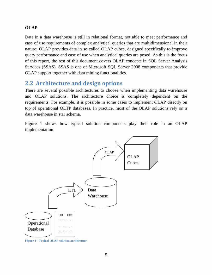
Figure 1 shows how typical solution components play their role in an OLAP
implementation.
Operational
Database
(OLTP)
Flat Files
---------
---------
---------
---------
---------
---------
---------
---------
Data
Warehouse
(Multidimensi
onal
Representatio
n)
OLAP
Cubes
ETL
OLAP
Proce
ss
Figure 1 - Typical OLAP solution architecture
6
3. SQL Server OLAP Solution Microsoft SQL Server 2008 is a modern DMBS supporting almost all recent data related
applications. SQL Server includes a number of data management and analysis
technologies. These technologies are: Database Engine, Analysis Services –
Multidimensional Data, Analysis Services – Data Mining, Integration Services,
Replication, Reporting Services and SQL Server Service broker.
If we want to introduce the same concepts as discussed in “Architecture and design
options”, in Figure 1, the Database would be replaced by SQL Server Database Engine,
ETL tool would be replaced with SSIS, data warehouse would be replaced by SQL
Server Database Engine. In 2.2”Architecture and design options” we also discussed that it
is possible to employ stand alone OLAP architectures. Similarly, however SSAS can be
used in standalone mode, usually it relies on other SQL server services to prepare data.
3.1 SQL Server Analysis Services (SSAS) SSAS provides two set of services and facilities, one for data mining and one for
multidimensional data. However they could be used totally separately, they can share
some components. For instance, it is possible that they use common data sources (or data
source views) and it is also possible that data mining algorithms use cubes to build data
mining models and/or apply them to data cubes.
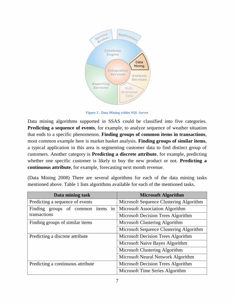
3.1.1 Data Mining Figure 2 (Data Mining 2008) shows how data mining facilities are provided within SQL
Server as a whole and also within SSAS.
7
Figure 2 - Data Mining within SQL Server
Data mining algorithms supported in SSAS could be classified into five categories.
Predicting a sequence of events, for example, to analyze sequence of weather situation
that ends to a specific phenomenon. Finding groups of common items in transactions,
most common example here is market basket analysis. Finding groups of similar items,
a typical application in this area is segmenting customer data to find distinct group of
customers. Another category is Predicting a discrete attribute, for example, predicting
whether one specific customer is likely to buy the new product or not. Predicting a
continuous attribute, for example, forecasting next month revenue.
(Data Mining 2008) There are several algorithms for each of the data mining tasks
mentioned above. Table 1 lists algorithms available for each of the mentioned tasks.
Data mining task Microsoft Algorithm
Predicting a sequence of events Microsoft Sequence Clustering Algorithm
Finding groups of common items in
transactions
Microsoft Association Algorithm
Microsoft Decision Trees Algorithm
Finding groups of similar items Microsoft Clustering Algorithm
Microsoft Sequence Clustering Algorithm
Predicting a discrete attribute Microsoft Decision Trees Algorithm
Microsoft Naive Bayes Algorithm
Microsoft Clustering Algorithm
Microsoft Neural Network Algorithm
Predicting a continuous attribute Microsoft Decision Trees Algorithm
Microsoft Time Series Algorithm
8
Table 1 - Microsoft Data Mining Algorithms and their respective tasks
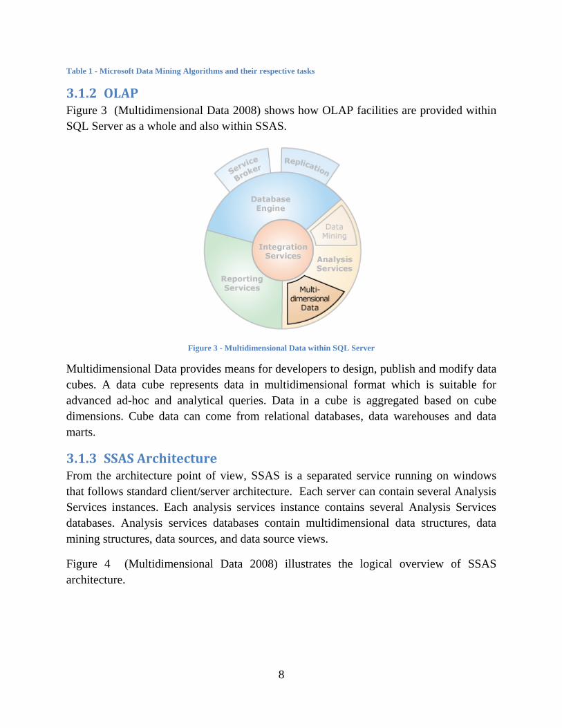
3.1.2 OLAP Figure 3 (Multidimensional Data 2008) shows how OLAP facilities are provided within
SQL Server as a whole and also within SSAS.
Figure 3 - Multidimensional Data within SQL Server
Multidimensional Data provides means for developers to design, publish and modify data
cubes. A data cube represents data in multidimensional format which is suitable for
advanced ad-hoc and analytical queries. Data in a cube is aggregated based on cube
dimensions. Cube data can come from relational databases, data warehouses and data
marts.
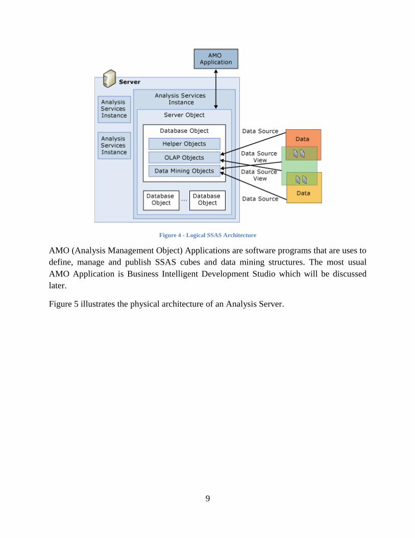
3.1.3 SSAS Architecture From the architecture point of view, SSAS is a separated service running on windows
that follows standard client/server architecture. Each server can contain several Analysis
Services instances. Each analysis services instance contains several Analysis Services
databases. Analysis services databases contain multidimensional data structures, data
mining structures, data sources, and data source views.
Figure 4 (Multidimensional Data 2008) illustrates the logical overview of SSAS
architecture.
9
Figure 4 - Logical SSAS Architecture
AMO (Analysis Management Object) Applications are software programs that are uses to
define, manage and publish SSAS cubes and data mining structures. The most usual
AMO Application is Business Intelligent Development Studio which will be discussed
later.
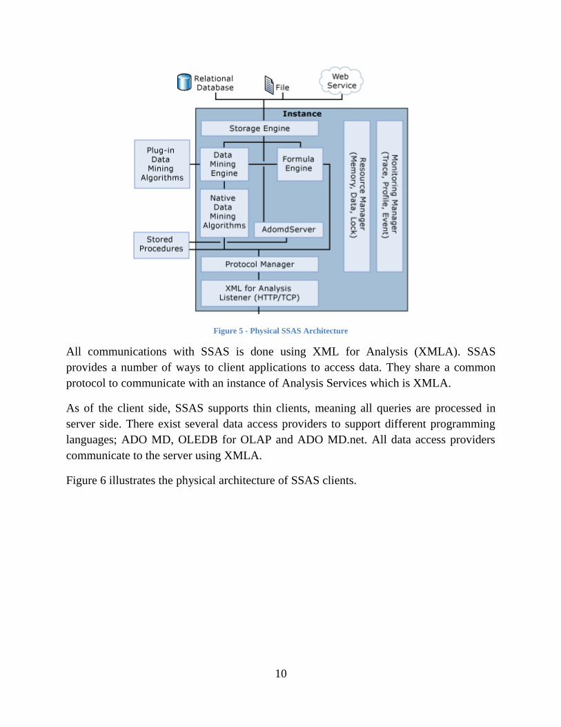
Figure 5 illustrates the physical architecture of an Analysis Server.
10
Figure 5 - Physical SSAS Architecture
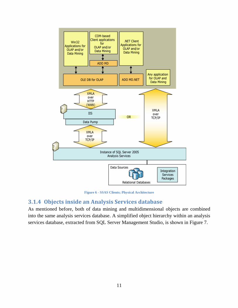
All communications with SSAS is done using XML for Analysis (XMLA). SSAS
provides a number of ways to client applications to access data. They share a common
protocol to communicate with an instance of Analysis Services which is XMLA.
As of the client side, SSAS supports thin clients, meaning all queries are processed in
server side. There exist several data access providers to support different programming
languages; ADO MD, OLEDB for OLAP and ADO MD.net. All data access providers
communicate to the server using XMLA.
Figure 6 illustrates the physical architecture of SSAS clients.
11
Figure 6 - SSAS Clients; Physical Architecture
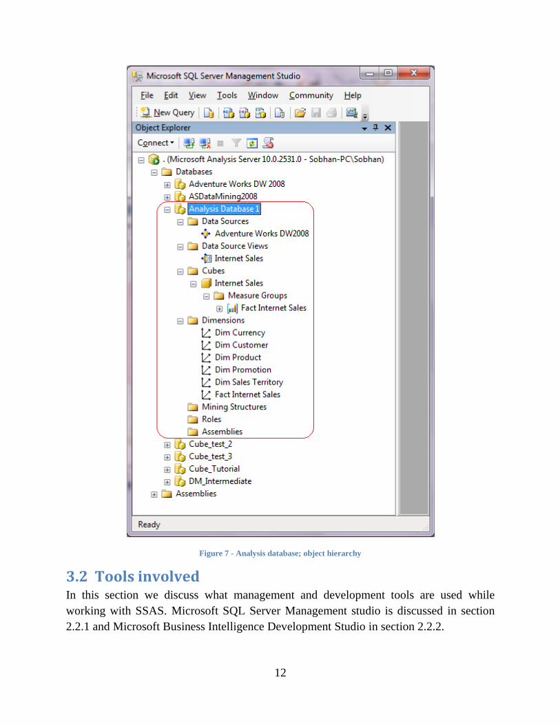
3.1.4 Objects inside an Analysis Services database As mentioned before, both of data mining and multidimensional objects are combined
into the same analysis services database. A simplified object hierarchy within an analysis
services database, extracted from SQL Server Management Studio, is shown in Figure 7.
12
Figure 7 - Analysis database; object hierarchy
3.2 Tools involved In this section we discuss what management and development tools are used while
working with SSAS. Microsoft SQL Server Management studio is discussed in section
2.2.1 and Microsoft Business Intelligence Development Studio in section 2.2.2.
13
3.2.1 SQL Server Management studio SQL Server Management Studio is a general management tool to manage relational
databases, Analysis Services databases, Reporting Services objects, and integration
services packages. By connecting SQL Server Management studio to an Analysis
Services instance on a machine, following database management tasks can be performed:
Processing analysis services objects
Processing an analysis services object means populating it with data. For example,
SQL Server Management studio provides the facilities to process data cubes,
which is populating them with data from data sources.
Browsing analysis services objects
The brows facility is a graphical query builder. By browsing, the content of
Analysis Services objects is queried. For example, browsing a cube includes
dragging attributes/hierarchies and cube measures to respective pane and brows
the data in the cube.
Constructing queries
Multidimensional queries (MDX), Data Mining queries (DMX) and XMLA
queries can be posed to Analysis Services database via SQL Server Management
studio.
Scripting Analysis Services objects
Scripting an object makes it an XMLA script so that it could be executed in
another analysis services instance to make the same object. Scripting only includes
structures and definitions. The data is provided after processing.
Managing Analysis Services Databases
Other general database management concepts are also included in SQL Server
Management Studio; Defining roles and security aspects of accessing the database
and making backups from analysis services databases.
3.2.2 Microsoft Business Intelligence Development Studio (BIDS) BIDS is the development environment for OLAP cubes and data mining models. BIDS is
Microsoft Visual Studio with Analysis Services projects extension. After development is
done, BIDS publishes the analysis services project to an Analysis Services database.
Processing the database can be performed both from BIDS and SQL Server Management
Studio.
Following are BIDS components that are used during development of Analysis Services
Projects:
14
Analysis Services Solution Explorer
The solution explorer show different objects within the analysis database that is
being developed. These include data sources, data source views, cubes,
dimensions, mining structures, roles, assemblies, and miscellaneous. By double
clicking on any item in the solution explorer, you can open that object with its
specific designer.
Analysis Services Designers
There are four designers in BIDS, Data Source View Designer, Cube Designer,
Dimension Designer, and Data Mining Designer. Some of these designers are
reviewed in this report while performing tutorials.
Analysis Services Menus
There are four menus related to analysis services projects, database menu, cube
menu, dimension menu and mining model menu. Each of these are activated when
the respective designer is open.
Analysis Services Tools/Options
The option menu provides some analysis services specific options on top of the general
ones: Connection and query timeouts, Default Deployment Server Edition, Default Target
Server, and Data Mining Viewers.
15
4. OLAP storage options When it comes to OLAP storage architecture, various ways of storing the
multidimensional data are proposed. The most common ones are Multidimensional
OLAP (MOLAP), Relational OLAP (ROLAP) and Hybrid OLAP (HOLAP). In this
section we start by defining the possible OLAP storage architectures, and then we discuss
all pre-defined storage settings in SSAS. Later we compare different storage scenarios.
This section ends with an example that shows how MDX queries are translated to SQL
queries when ROLAP storage is used.
4.1 MOLAP, HOLAP and ROALP ROLAP stores data in relational tables. If ROLAP is used as storage mode, there is no
need to transfer the data from relational to none relational systems. Therefore ROLAP is
in fact an abstraction level over relational data that provides multidimensional query
support.
In contrast with ROLAP, MOLAP stores cube data in multidimensional array format.
This requires pre-computation and storage of data in the cube, therefore a procedure
called processing needs to be done to populate cube with latest data.
HOLAP is a popular which stands between ROLAP and MOLAP. In HOLAP, depending
on the OLAP storage designer facilities, developer can choose which part of data to keep
in relational format and which parts in multidimensional. This allows developers to
utilize fast MOLAP query response and scalability of ROLAP at the same time.
4.2 The pre-defined storage settings Although manual configuration is possible to configure details of storage settings in
SSAS, some predefined storage settings are developed to help users. These storage
settings can be configured separately for any dimension and any measure group (fact
table data) within a cube. Following are predefined storage settings in SSAS.
MOLAP
o Measure group data and aggregations are stored in multidimensional
format.
o Notifications are not received when data changes.
o Processing must be either scheduled or performed manually.
Scheduled MOLAP
16
o Measure group data and aggregations are stored in multidimensional
format.
o Notifications are not received when data changes.
o Processing is automatically performed every 24 hours.
Automatic MOLAP
o Measure group data and aggregations are stored in multidimensional
format.
o The server will listen for notifications when data changes.
o Processing is performed automatically with no restriction on latency.
Medium-latency MOLAP
o Measure group data and aggregations are stored in multidimensional
format.
o The server will listen for notifications when data changes.
o Processing is performed automatically with a target latency of four hours.
Low-latency MOLAP
o Measure group data and aggregations are stored in multidimensional
format.
o The server will listen for notifications when data changes.
o Processing is performed automatically with a target latency of 30 minutes.
Real-time HOLAP
o Measure group data is maintained in a relational format, and aggregations
are stored in multidimensional format.
o The server will listen for notifications when data changes.
o All Queries reflect the current state of data.
Real-time ROLAP
o Measure group data and aggregations are stored in relational format.
o The server will listen for notifications when data changes.
o All Queries reflect the current state of data.
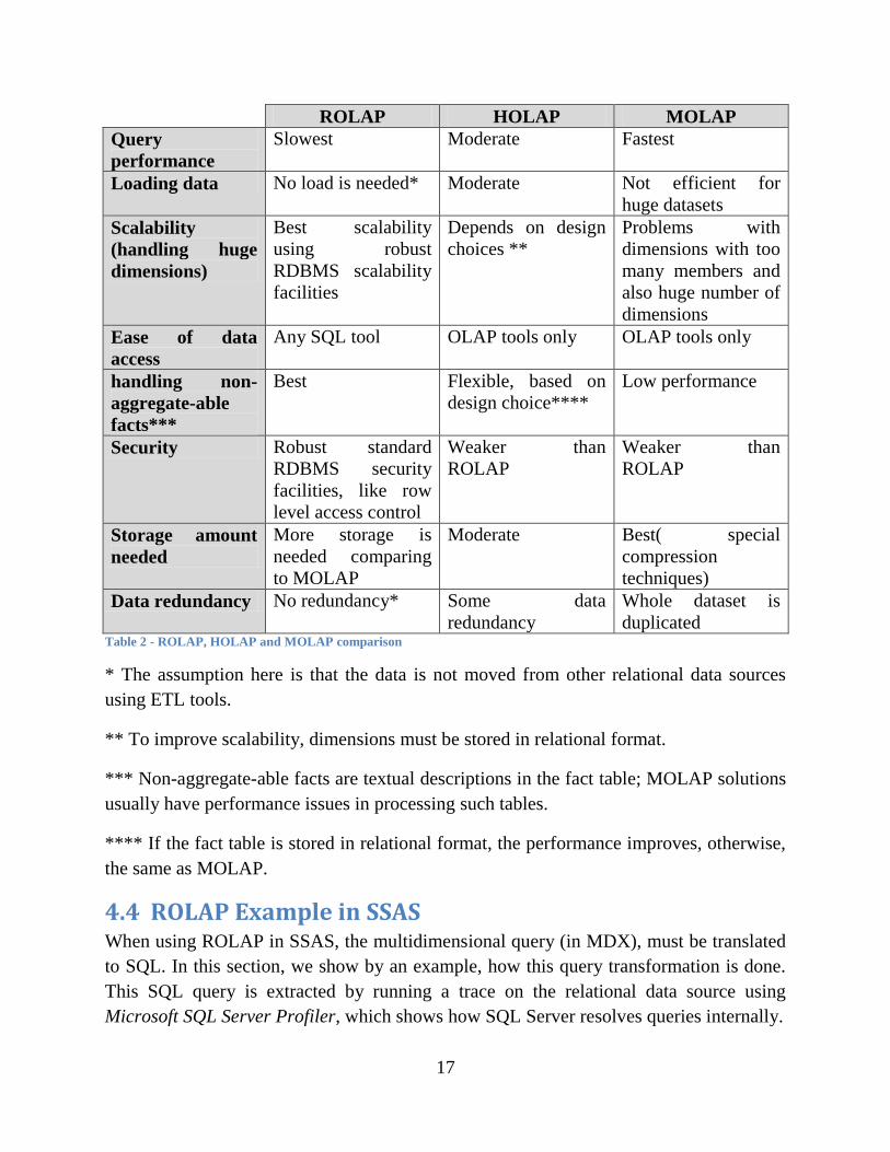
4.3 Comparison between ROLAP, HOLAP and MOLAP (ROLAP 2010) Each of the storage options discussed so far has its own advantages and
disadvantages. Table 2 summarizes advantages and disadvantages of each storage setting.
17
ROLAP HOLAP MOLAP
Query
performance
Slowest Moderate Fastest
Loading data No load is needed* Moderate Not efficient for
huge datasets
Scalability
(handling huge
dimensions)
Best scalability
using robust
RDBMS scalability
facilities
Depends on design
choices **
Problems with
dimensions with too
many members and
also huge number of
dimensions
Ease of data
access
Any SQL tool OLAP tools only OLAP tools only
handling non-
aggregate-able
facts***
Best Flexible, based on
design choice****
Low performance
Security Robust standard
RDBMS security
facilities, like row
level access control
Weaker than
ROLAP
Weaker than
ROLAP
Storage amount
needed
More storage is
needed comparing
to MOLAP
Moderate Best( special
compression
techniques)
Data redundancy No redundancy* Some data
redundancy
Whole dataset is
duplicated Table 2 - ROLAP, HOLAP and MOLAP comparison
* The assumption here is that the data is not moved from other relational data sources
using ETL tools.
** To improve scalability, dimensions must be stored in relational format.
*** Non-aggregate-able facts are textual descriptions in the fact table; MOLAP solutions
usually have performance issues in processing such tables.
**** If the fact table is stored in relational format, the performance improves, otherwise,
the same as MOLAP.
4.4 ROLAP Example in SSAS When using ROLAP in SSAS, the multidimensional query (in MDX), must be translated
to SQL. In this section, we show by an example, how this query transformation is done.
This SQL query is extracted by running a trace on the relational data source using
Microsoft SQL Server Profiler, which shows how SQL Server resolves queries internally.
18
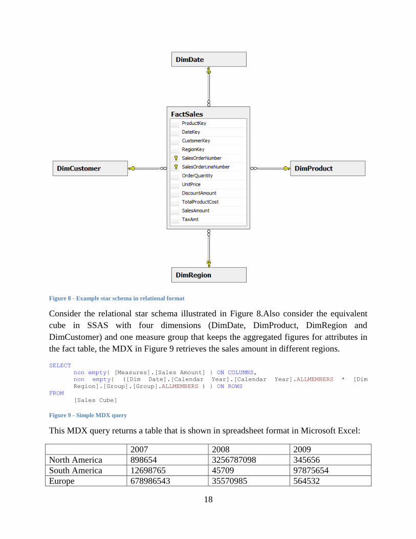
Figure 8 - Example star schema in relational format
Consider the relational star schema illustrated in Figure 8.Also consider the equivalent
cube in SSAS with four dimensions (DimDate, DimProduct, DimRegion and
DimCustomer) and one measure group that keeps the aggregated figures for attributes in
the fact table, the MDX in Figure 9 retrieves the sales amount in different regions.
SELECT
non empty{ [Measures].[Sales Amount] } ON COLUMNS,
non empty{ ([Dim Date].[Calendar Year].[Calendar Year].ALLMEMBERS * [Dim
Region].[Group].[Group].ALLMEMBERS ) } ON ROWS
FROM
[Sales Cube]
Figure 9 - Simple MDX query
This MDX query returns a table that is shown in spreadsheet format in Microsoft Excel:
2007 2008 2009
North America 898654 3256787098 345656
South America 12698765 45709 97875654
Europe 678986543 35570985 564532
19
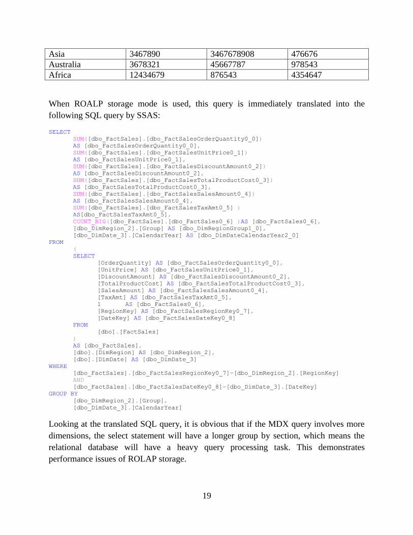
Asia 3467890 3467678908 476676
Australia 3678321 45667787 978543
Africa 12434679 876543 4354647
When ROALP storage mode is used, this query is immediately translated into the
following SQL query by SSAS:
SELECT
SUM([dbo_FactSales].[dbo_FactSalesOrderQuantity0_0])
AS [dbo_FactSalesOrderQuantity0_0],
SUM([dbo_FactSales].[dbo_FactSalesUnitPrice0_1])
AS [dbo_FactSalesUnitPrice0_1],
SUM([dbo_FactSales].[dbo_FactSalesDiscountAmount0_2])
AS [dbo_FactSalesDiscountAmount0_2],
SUM([dbo_FactSales].[dbo_FactSalesTotalProductCost0_3])
AS [dbo_FactSalesTotalProductCost0_3],
SUM([dbo_FactSales].[dbo_FactSalesSalesAmount0_4])
AS [dbo_FactSalesSalesAmount0_4],
SUM([dbo_FactSales].[dbo_FactSalesTaxAmt0_5] )
AS[dbo_FactSalesTaxAmt0_5],
COUNT_BIG([dbo_FactSales].[dbo_FactSales0_6] )AS [dbo_FactSales0_6],
[dbo_DimRegion_2].[Group] AS [dbo_DimRegionGroup1_0],
[dbo_DimDate_3].[CalendarYear] AS [dbo_DimDateCalendarYear2_0]
FROM
(
SELECT
[OrderQuantity] AS [dbo_FactSalesOrderQuantity0_0],
[UnitPrice] AS [dbo_FactSalesUnitPrice0_1],
[DiscountAmount] AS [dbo_FactSalesDiscountAmount0_2],
[TotalProductCost] AS [dbo_FactSalesTotalProductCost0_3],
[SalesAmount] AS [dbo_FactSalesSalesAmount0_4],
[TaxAmt] AS [dbo_FactSalesTaxAmt0_5],
1 AS [dbo_FactSales0_6],
[RegionKey] AS [dbo_FactSalesRegionKey0_7],
[DateKey] AS [dbo_FactSalesDateKey0_8]
FROM
[dbo].[FactSales]
)
AS [dbo_FactSales],
[dbo].[DimRegion] AS [dbo_DimRegion_2],
[dbo].[DimDate] AS [dbo_DimDate_3]
WHERE
[dbo_FactSales].[dbo_FactSalesRegionKey0_7]=[dbo_DimRegion_2].[RegionKey]
AND
[dbo_FactSales].[dbo_FactSalesDateKey0_8]=[dbo_DimDate_3].[DateKey]
GROUP BY
[dbo_DimRegion_2].[Group],
[dbo_DimDate_3].[CalendarYear]
Looking at the translated SQL query, it is obvious that if the MDX query involves more
dimensions, the select statement will have a longer group by section, which means the
relational database will have a heavy query processing task. This demonstrates
performance issues of ROLAP storage.
20
5. Scalability test In this section the scalability of ROLAP storage in SSAS is evaluated. A test database
was created, following star schema convention. An OLAP cube was designed based on
the star schema. Then new records were added to the system in buckets. After each
bucket was inserted, a test query was posed to SSAS to measure the response time.
5.1 Test platform Scalability test was conducted on Microsoft Windows 7 professional operating system,
SQL Server 2008 (Developer version) database engine and on laptop PC with 4GB ram
and Intel Core™ 2 Duo P8700 (2.53GHz) CPU.
5.2 Test data and storage options Database schema used for this test is identical to Figure 8. The query used is also the
same as the query in Figure 9. The storage option used in this test is Real-time ROLAP,
described in “The pre-defined storage settings”.
Following table summarizes the test data size at the end of test.
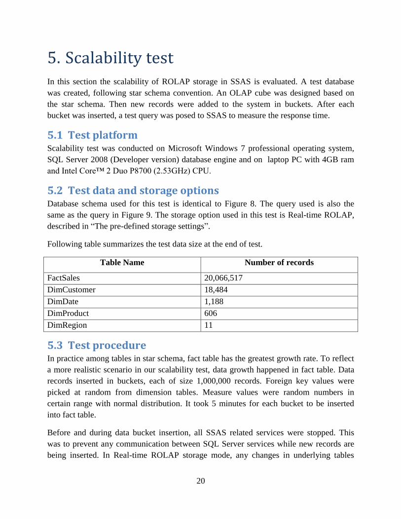
Table Name Number of records
FactSales 20,066,517
DimCustomer 18,484
DimDate 1,188
DimProduct 606
DimRegion 11
5.3 Test procedure In practice among tables in star schema, fact table has the greatest growth rate. To reflect
a more realistic scenario in our scalability test, data growth happened in fact table. Data
records inserted in buckets, each of size 1,000,000 records. Foreign key values were
picked at random from dimension tables. Measure values were random numbers in
certain range with normal distribution. It took 5 minutes for each bucket to be inserted
into fact table.
Before and during data bucket insertion, all SSAS related services were stopped. This
was to prevent any communication between SQL Server services while new records are
being inserted. In Real-time ROLAP storage mode, any changes in underlying tables
21
causes notifications to go from data source to SSAS. If SSAS services were running, the
insertion time would have become much longer.
Since the same query was posed to SSAS after each bucket insertion, SSAS service was
restarted to eliminate any caching mechanism. This way the query optimizer is forced to
re-build execution plan of each individual query and is to avoid the chance of using any
intermediate results from previous query executions.
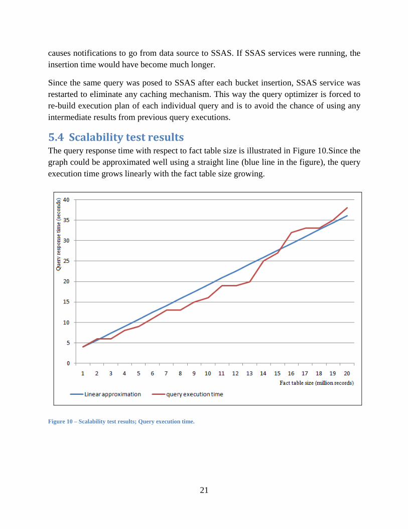
5.4 Scalability test results The query response time with respect to fact table size is illustrated in Figure 10.Since the
graph could be approximated well using a straight line (blue line in the figure), the query
execution time grows linearly with the fact table size growing.
Figure 10 – Scalability test results; Query execution time.
22
6. Summary Microsoft SQL Server has robust capabilities for development, maintenance and querying
of OLAP cubes. SSAS provides the combination of flexible architecture and robust user-
friendly tools. The OLAP storage settings provide adequate options for system designers.
SSAS flexible architecture makes it possible to integrate SSAS with any type of data
source, and any means of end user interaction. Since OLAP is additional to basic
database technologies and IT solutions, there are always other database related
technologies and user interfaces that OLAP has to integrate to. SSAS architecture
flexibility makes it easier to integrate OLAP with existing database and interface
technologies.
SQL Server provides user friendly development tools. Business Intelligence
Development Studio (BIDS) is based on Microsoft Visual Studio 2008, one of the most
popular and user friendly development environments. Since BIDS has been used in other
Microsoft products before, it has become mature enough to facilitate OLAP development
and design.
SSAS gives many options to architecture designers to propose problem specific OLAP
storage solutions. There are seven predefined OLAP storage options. Each of them is
designed for specific applications. In addition to predefined storage options, architecture
designers are given the chance to define even more specific storage options based on
particular application.
The scalability test reveals that query response time grows linearly with the database size.
As the main purpose behind OLAP is to support ad-hoc queries, the linear complexity is a
major problem in applications with huge data. On the other hand, real time queries
capabilities provided by ROLAP storage mode could be very helpful if the database size
is moderate.
23
7. Appendix A – Making cube tutorial
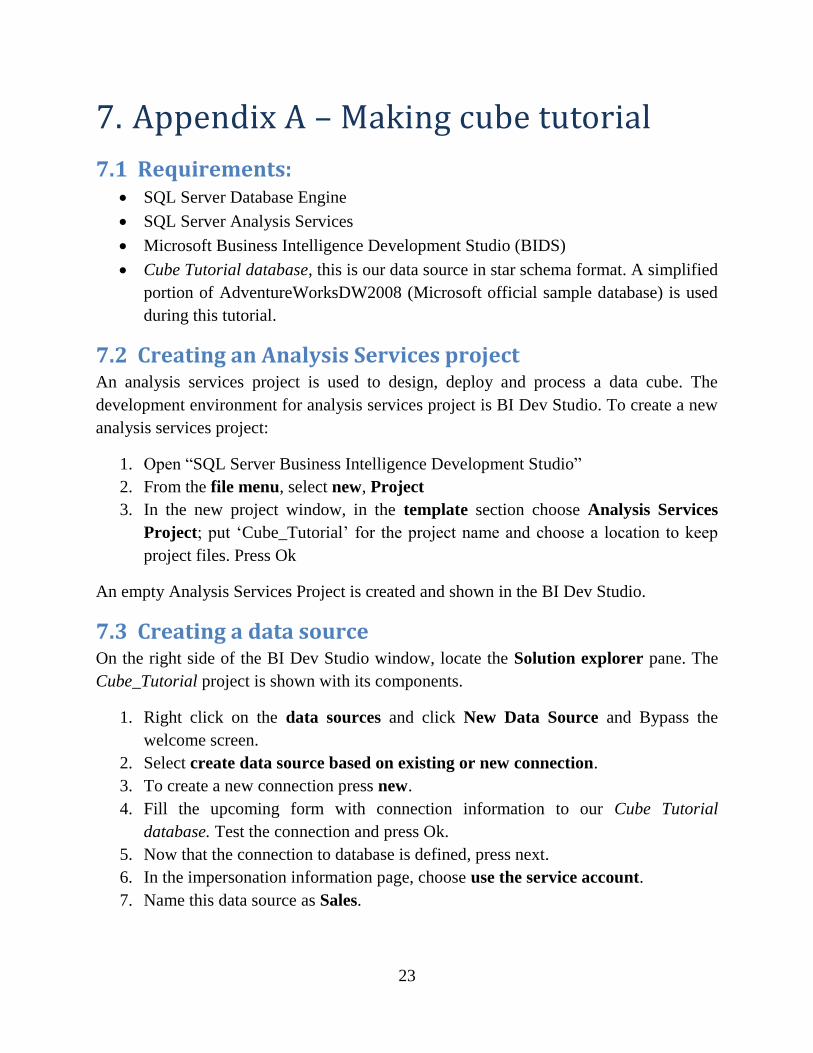
7.1 Requirements: SQL Server Database Engine
SQL Server Analysis Services
Microsoft Business Intelligence Development Studio (BIDS)
Cube Tutorial database, this is our data source in star schema format. A simplified
portion of AdventureWorksDW2008 (Microsoft official sample database) is used
during this tutorial.
7.2 Creating an Analysis Services project An analysis services project is used to design, deploy and process a data cube. The
development environment for analysis services project is BI Dev Studio. To create a new
analysis services project:
1. Open “SQL Server Business Intelligence Development Studio”
2. From the file menu, select new, Project
3. In the new project window, in the template section choose Analysis Services
Project; put „Cube_Tutorial‟ for the project name and choose a location to keep
project files. Press Ok
An empty Analysis Services Project is created and shown in the BI Dev Studio.
7.3 Creating a data source On the right side of the BI Dev Studio window, locate the Solution explorer pane. The
Cube_Tutorial project is shown with its components.
1. Right click on the data sources and click New Data Source and Bypass the
welcome screen.
2. Select create data source based on existing or new connection.
3. To create a new connection press new.
4. Fill the upcoming form with connection information to our Cube Tutorial
database. Test the connection and press Ok.
5. Now that the connection to database is defined, press next.
6. In the impersonation information page, choose use the service account.
7. Name this data source as Sales.
24
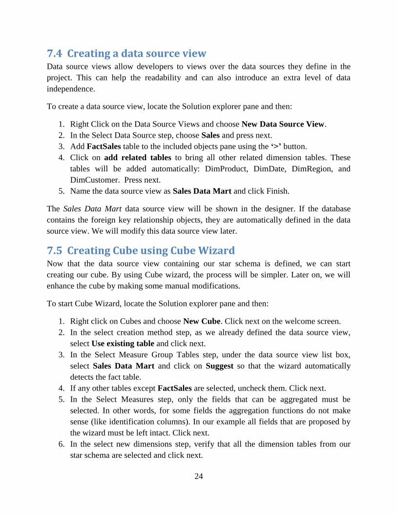
7.4 Creating a data source view Data source views allow developers to views over the data sources they define in the
project. This can help the readability and can also introduce an extra level of data
independence.
To create a data source view, locate the Solution explorer pane and then:
1. Right Click on the Data Source Views and choose New Data Source View.
2. In the Select Data Source step, choose Sales and press next.
3. Add FactSales table to the included objects pane using the ‘>’ button.
4. Click on add related tables to bring all other related dimension tables. These
tables will be added automatically: DimProduct, DimDate, DimRegion, and
DimCustomer. Press next.
5. Name the data source view as Sales Data Mart and click Finish.
The Sales Data Mart data source view will be shown in the designer. If the database
contains the foreign key relationship objects, they are automatically defined in the data
source view. We will modify this data source view later.
7.5 Creating Cube using Cube Wizard Now that the data source view containing our star schema is defined, we can start
creating our cube. By using Cube wizard, the process will be simpler. Later on, we will
enhance the cube by making some manual modifications.
To start Cube Wizard, locate the Solution explorer pane and then:
1. Right click on Cubes and choose New Cube. Click next on the welcome screen.
2. In the select creation method step, as we already defined the data source view,
select Use existing table and click next.
3. In the Select Measure Group Tables step, under the data source view list box,
select Sales Data Mart and click on Suggest so that the wizard automatically
detects the fact table.
4. If any other tables except FactSales are selected, uncheck them. Click next.
5. In the Select Measures step, only the fields that can be aggregated must be
selected. In other words, for some fields the aggregation functions do not make
sense (like identification columns). In our example all fields that are proposed by
the wizard must be left intact. Click next.
6. In the select new dimensions step, verify that all the dimension tables from our
star schema are selected and click next.
25
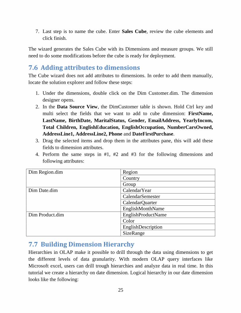
7. Last step is to name the cube. Enter Sales Cube, review the cube elements and
click finish.
The wizard generates the Sales Cube with its Dimensions and measure groups. We still
need to do some modifications before the cube is ready for deployment.
7.6 Adding attributes to dimensions The Cube wizard does not add attributes to dimensions. In order to add them manually,
locate the solution explorer and follow these steps:
1. Under the dimensions, double click on the Dim Customer.dim. The dimension
designer opens.
2. In the Data Source View, the DimCustomer table is shown. Hold Ctrl key and
multi select the fields that we want to add to cube dimension: FirstName,
LastName, BirthDate, MaritalStatus, Gender, EmailAddress, YearlyIncom,
Total Children, EnglishEducation, EnglishOccupation, NumberCarsOwned,
AddressLine1, AddressLine2, Phone and DateFirstPurchase.
3. Drag the selected items and drop them in the attributes pane, this will add these
fields to dimension attributes.
4. Perform the same steps in #1, #2 and #3 for the following dimensions and
following attributes:
Dim Region.dim Region
Country
Group
Dim Date.dim CalendarYear
CalendarSemester
CalendarQuarter
EnglishMonthName
Dim Product.dim EnglishProductName
Color
EnglishDescription
SizeRange
7.7 Building Dimension Hierarchy Hierarchies in OLAP make it possible to drill through the data using dimensions to get
the different levels of data granularity. With modern OLAP query interfaces like
Microsoft excel, users can drill trough hierarchies and analyze data in real time. In this
tutorial we create a hierarchy on date dimension. Logical hierarchy in our date dimension
looks like the following:
26
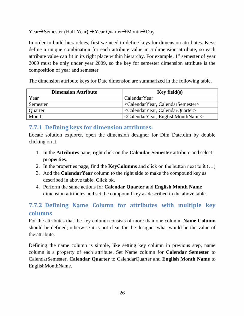
YearSemester (Half Year) Year QuarterMonthDay
In order to build hierarchies, first we need to define keys for dimension attributes. Keys
define a unique combination for each attribute value in a dimension attribute, so each
attribute value can fit in its right place within hierarchy. For example, 1st semester of year
2009 must be only under year 2009, so the key for semester dimension attribute is the
composition of year and semester.
The dimension attribute keys for Date dimension are summarized in the following table.
Dimension Attribute Key field(s)
Year CalendarYear
Semester <CalendarYear, CalendarSemester>
Quarter <CalendarYear, CalendarQuarter>
Month <CalendarYear, EnglishMonthName>
7.7.1 Defining keys for dimension attributes: Locate solution explorer, open the dimension designer for Dim Date.dim by double
clicking on it.
1. In the Attributes pane, right click on the Calendar Semester attribute and select
properties.
2. In the properties page, find the KeyColumns and click on the button next to it (…)
3. Add the CalendarYear column to the right side to make the compound key as
described in above table. Click ok.
4. Perform the same actions for Calendar Quarter and English Month Name
dimension attributes and set the compound key as described in the above table.
7.7.2 Defining Name Column for attributes with multiple key
columns For the attributes that the key column consists of more than one column, Name Column
should be defined; otherwise it is not clear for the designer what would be the value of
the attribute.
Defining the name column is simple, like setting key column in previous step, name
column is a property of each attribute. Set Name column for Calendar Semester to
CalendarSemester, Calendar Quarter to CalendarQuarter and English Month Name to
EnglishMonthName.
27
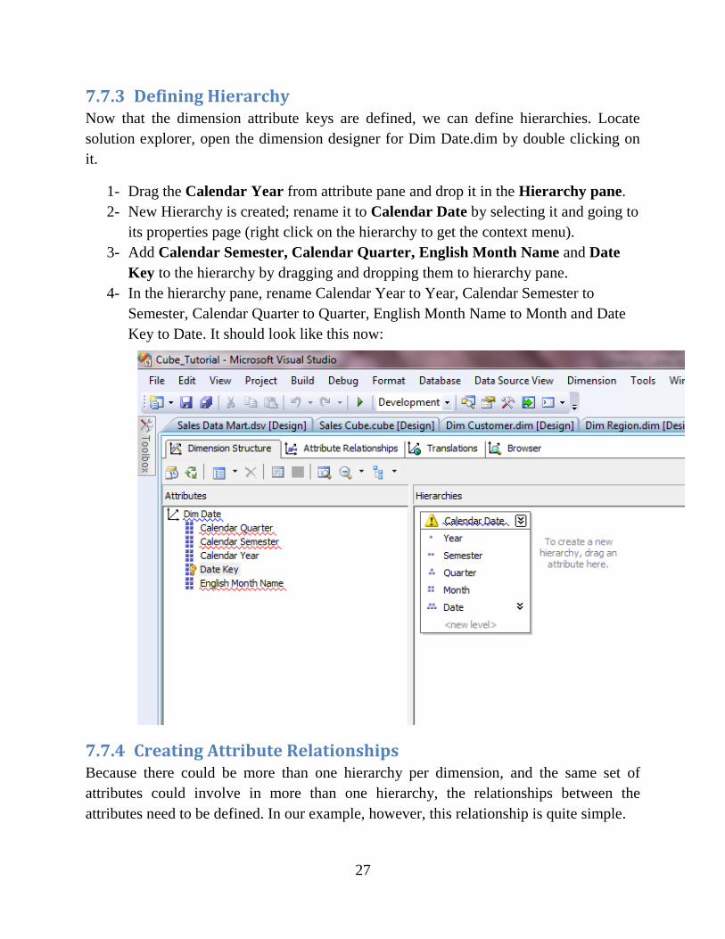
7.7.3 Defining Hierarchy Now that the dimension attribute keys are defined, we can define hierarchies. Locate
solution explorer, open the dimension designer for Dim Date.dim by double clicking on
it.
1- Drag the Calendar Year from attribute pane and drop it in the Hierarchy pane.
2- New Hierarchy is created; rename it to Calendar Date by selecting it and going to
its properties page (right click on the hierarchy to get the context menu).
3- Add Calendar Semester, Calendar Quarter, English Month Name and Date
Key to the hierarchy by dragging and dropping them to hierarchy pane.
4- In the hierarchy pane, rename Calendar Year to Year, Calendar Semester to
Semester, Calendar Quarter to Quarter, English Month Name to Month and Date
Key to Date. It should look like this now:
7.7.4 Creating Attribute Relationships Because there could be more than one hierarchy per dimension, and the same set of
attributes could involve in more than one hierarchy, the relationships between the
attributes need to be defined. In our example, however, this relationship is quite simple.
28
To define the attribute relationships in Date Dimension, Open the dimension designer and
click on the Attribute Relationships tab (Right side of the Dimension Structure tab).
7.8 Deploying the Cube and processing it Now the cube is ready to be deployed and processed. Microsoft Analysis Server
maintains all objects related to an Analysis Services Project as well as their data items. In
the deployment process design structures and data definitions are deployed to the server.
On the other hand, processing fills the structure with data.
Every time the cube structure changes, or new data needs to be populated into cube, the
deployment and processing has to be done respectively.
Too change the deployment options, right click on the project name in the solution
explorer and choose properties. By choosing Deployment in the left pane of the property
page, the deployment options, such as Server and Database are shown and can be
altered.
To deploy the project, open the Debug menu and choose Start Debugging.
To process the database, open the Database menu and press Process, then press Run.
The process progress window shows the progress.
7.9 Brows Cube Data When the cube is deployed and processed, the cube data could be browsed using various
OLAP tools. One of the easiest and fastest tools for the developers is already available in
BI Dev Studio.
In order to access the BI Dev Studio browser, locate the Solution Explorer pain, select
the cube from cubes folder and double click on it. The cube designer opens. The last tab
in the cube designer is Browser.
The tool is self explaining and easy to use: On the left pane, the data items are available
and can be drag/dropped to the right panes. The top right pane is for adding filters, while
the bottom pane is the Data pane.
As an example, add the Sales Amount from measure to the data pane, add Calendar
Date hierarchy from Dim Date to the place labeled as „Drop Row Fields Here‟ in data
pane and add Group from Dim Region hierarchy to the place labeled as „Drop Column
Fields Here‟ in data pane.

29
Try opening/closing the + and - signs next to each year and drill trough the hierarchy we
created in the tutorial.
30
8. Bibliography Data Mining, Microsoft. "SQL Server Analysis Services - Data Mining." Microsoft
TechNet. 2008. http://technet.microsoft.com/en-us/library/bb510517.aspx (accessed April
20, 2010).
Inmon, W.H. "What is a Data wareouse?" Prism, Volume 1, Number 1, 1995.
Multidimensional Data, Microsoft. "SQL Server Analysis Services - Multidimensional
Data." Microsoft TechNet. 2008. http://technet.microsoft.com/en-
us/library/bb522607.aspx (accessed April 20, 2010).
ROLAP, Wikipedia. Wikipedia. 2010. http://en.wikipedia.org/wiki/ROLAP (accessed
May 01, 2010).