Embed Size (px)
Citation preview
FACULTEIT WETENSCHAPPEN
Opleiding Master of Science in de geologie
Academiejaar 2013–2014
Scriptie voorgelegd tot het behalen van de graad
Van Master of Science in de geologie
Promotor: Dr. S. Bertrand
Begeleider: Dr. S. Bertrand
Leescommissie: Prof. Dr. M. De Batist, Dr. V. Heyvaert
Mineralogy and geochemistry of north Patagonian river sediments: Influence of provenance and weathering processes
Toon Van Dijck

Cover picture: Rio Baker, close to Lago Bertrand. (Photo: Dr. S. Bertrand)

Acknowledgements
I would like to seize the opportunity here to thank some people that helped me completing
this project.
Most importantly I would like to thank my promotor Dr. Sebastien Bertrand. First and for all
for the great subject he proposed, but most of all for the help I received from him. His door
was always open if I needed some information, help, or when I was stuck with something. He
also made time to read and correct the chapters I would send him.
I would also like to thank the people of the Renard Centre of Marine Geology for letting me
use their laboratory, their lab equipment, and their computers. They also organized sessions
to get started with some software programs. I also thank the lab technicians of the Van
Ranst lab for letting me use their centrifuge.
Furthermore I also want to thank Prof. Fagel and Joël Otten, from the Université de Liège,
for the help during the XRD measurements, especially for running my samples during the
night.
Last but not least, I would like to thank Sanne, for supporting and motivating me while I was
writing this MSc thesis.

Table of contents
1. Introduction .................................................................................................................. 1
2. General Setting ............................................................................................................. 3
2.1 Introduction .......................................................................................................................... 3
2.2. Geological Setting ................................................................................................................ 5
2.2.1. Andean Cordillera ......................................................................................................... 5
2.2.2. Geology of Patagonia ................................................................................................... 6
2.2.3. Soils............................................................................................................................... 7
2.3. Climatic Setting .................................................................................................................... 8
2.3.1. Present-day climate ..................................................................................................... 8
2.4. Late Quaternary evolution ................................................................................................ 11
2.4.1 Climate and glacier fluctuations .................................................................................. 11
2.4.2. Volcanic activity .......................................................................................................... 14
2.4.3. River discharge ........................................................................................................... 17
3. Weathering Processes ................................................................................................. 19
3.1. Introduction ....................................................................................................................... 19
3.2. Physical Weathering .......................................................................................................... 19
3.2.1. Frost Weathering........................................................................................................ 19
3.2.2. Salt Weathering .......................................................................................................... 20
3.2.3. Insolation Weathering ................................................................................................ 20
3.2.4. Pressure-Release Weathering .................................................................................... 20
3.2.5. Wetting and Drying .................................................................................................... 20
3.3. Chemical Weathering ........................................................................................................ 21
3.3.1. Dissolution .................................................................................................................. 21
3.3.2. Hydration .................................................................................................................... 22
3.3.3. Carbonation ................................................................................................................ 22
3.3.4. Hydrolysis ................................................................................................................... 22
3.3.5. Oxidation-Reduction (Redox) Processes .................................................................... 23
3.3.6. Exchangeable Ions ...................................................................................................... 23
3.4. Biological Weathering ....................................................................................................... 23
3.4.1. Biophysical Weathering .............................................................................................. 24
3.4.2. Biochemical Weathering ............................................................................................ 24
3.5. Factors Controlling Weathering ........................................................................................ 25
3.6. Weathering in Patagonia ................................................................................................... 26
3.6.1. Bedrock ....................................................................................................................... 26
3.6.2. Soils............................................................................................................................. 27
4. Material & Methods .................................................................................................... 28
4.1. Samples and data obtained prior to this study ................................................................. 28
4.1.1. River sediment samples ............................................................................................. 28
4.1.2. Geochemical Data ...................................................................................................... 29
4.1.3. Watersheds ................................................................................................................ 29
4.2. Sediment sample preparation ........................................................................................... 30
4.2.1. Freeze-drying .............................................................................................................. 30
4.2.2. Sieving ........................................................................................................................ 31
4.2.3. Atterberg Column ....................................................................................................... 32
4.3. X-Ray Diffraction (XRD) ..................................................................................................... 33
4.3.1 Analytical procedure ................................................................................................... 33
4.3.2 Semi-quantification using EVA .................................................................................... 34
4.3.3. Quantification using RockJock.................................................................................... 35
4.4. Statistical Analysis ............................................................................................................. 37
4.5. Cartography ....................................................................................................................... 38
5. Results ........................................................................................................................ 41
5.1 Sediment Analysis .............................................................................................................. 41
5.1.1. Grain size distribution ................................................................................................ 41
5.1.2. X-Ray Diffraction (XRD) analyses with Eva ................................................................. 42
5.1.3. X-Ray Diffraction (XRD) analyses with RockJock ........................................................ 46
5.2. Simplified Geological Maps ............................................................................................... 51
5.3. Characteristics of the watersheds ..................................................................................... 54
5.3.1. Glacier coverage ......................................................................................................... 54
5.3.2. Volcanic ash soil coverage .......................................................................................... 54
5.3.3. Lithological abundances ............................................................................................. 55
6. Discussion ................................................................................................................... 56
6.1. XRD quantification techniques .......................................................................................... 56
6.1.1. Comparison between EVA and RockJock results ....................................................... 56
6.1.2. Selection of the most appropriate quantification technique .................................... 58
6.2. Relations between mineralogy and grain size .................................................................. 59
6.3. Relations between mineralogy and geochemistry............................................................ 61
6.4. Factors (other than grain size) affecting sediment geochemistry and mineralogy .......... 65
6.5. Provenance and weathering ............................................................................................. 68
6.5 Representativeness of the < 88 µm sample ....................................................................... 71
7. Conclusions ................................................................................................................. 72
8. References .................................................................................................................. 74
Dutch summary .............................................................................................................. 81
Appendix A: Geochemical data ....................................................................................... 86
Appendix B: XRD EVA results .......................................................................................... 89
Appendix C: XRD RockJock results ................................................................................... 92
Appendix D: Mineralogy and grain size............................................................................ 95
1
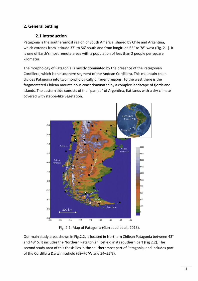
1. Introduction
Climate change recently became the hottest topic in Quaternary geology. Global warming
affects countless processes, which are changing at an alarming rate, on the Earth’s surface
and in the oceans. It is important that not only climate changes itself, and its causes, are well
understood, but also the effects of climate change need to be investigated. Rivers are part of
this constantly changing system, driven by changing climate. The rivers drain the Earth’s
surface towards the ocean. Changing climatic environments will cause other processes to
dominate erosion and weathering, resulting in compositionally and quantitatively distinct
material that is transported through rivers to the oceans, which in turn affects the
biogeochemistry, aquatic productivity, and ultimately fisheries. Therefore it is important to
understand the processes of weathering and erosion that contribute to, and are carried out
by, the river system.
The main goal of this project is to determine the provenance of Patagonian river sediments
and to obtain insights in the weathering processes that influence their composition.
Research on provenance and weathering are relatively common, but for Patagonia these
studies are scarce (e.g. Lee et al., 2013). Patagonia is not only attractive for adventurers and
explorers but it is also an area of great interest for scientists. Unlike the northern
hemisphere, the southern hemisphere is mostly occupied by the oceans so regions to carry
out climate-related research are rare. This is why research in Patagonia can give important
insights in, and evidence for global past and present climatic models.
This study will use seven river sediment samples, from which six are located in northern
Patagonia (4348°S) and one in southernmost Patagonia (5455°S), collected by Bertrand et
al. (2009; 2011). The samples will be separated into different grain size fractions by
combining dry sieving and Atterberg – Stokes separation. This may give us the possibility to
study mineralogical variations with grain size. The identification and quantification of the
mineralogy of the samples will be based on X-Ray Diffraction (XRD) measurements. Because
XRD a is semi-quantification technique, two methods will be used and compared to
determine and quantify the minerals present in the samples. The first one is a manual
method which uses the EVA – Bruker software and the second method will be done with
RockJock, an automated XRD determination and quantification program. Geochemical data
is available for five of the seven samples (Bertrand et al., 2012). It will be used to investigate
the relation between geochemistry and mineralogy in our samples.
To obtain insights on the provenance of the sediments, and the weathering processes that
influence their composition, information about the watersheds of the rivers is necessary. A
simplified geological map of the area will be constructed. This is necessary because for this
study, only the differences in lithology are meaningful. The age of the geological units is not
important. The abundances of the lithologies in each watershed will be determined. The
presence of soils, and their characteristics will also be investigated. Other factors that could
2
have an influence on the mineralogical composition of the river sediment samples are
precipitation, river dynamics, the presence of glaciers and ice fields, and volcanic ash
deposits (since active volcanoes are present in our study area). We will try to determine the
influence of all these factors on the mineralogical composition of our samples.
Additionally, the representativeness of the <88 µm fraction will be investigated. The <88 µm
fraction is often used to represent the sediment that is effectively transported in suspension
by rivers (e.g. Bertrand, 2009). For our study, the samples will be separated in grain size
fractions, from which seven fractions are smaller than <88 µm. <88 µm samples are also
available for each river sediment sample. Therefore it is possible to check which fractions are
mostly represented in the <88 µm fraction, by including the <88 µm samples in the XRD
measurements.
This thesis will start with a general setting of the study area in the second chapter. This
includes the geological background of the southern Andes, the geology of our study area,
the current climatic conditions in Patagonia, and also a subchapter about the Late-
Quaternary evolution of the region. Since weathering processes will have an important
influence on the mineralogy of the samples, a classification of the different weathering
processes is given in chapter 3. The factors that control weathering and weathering
conditions in Patagonia are also discussed in this chapter. Chapter 4 is the “Materials and
Methods” chapter. This chapter describes the available data, the methods that are used to
analyze the samples, the analytical methods, and the process of digitalizing and modifying
maps. The results are presented in the next chapter and the interpretation and discussion is
given in chapter 6. In this “Discussion” chapter, a comparison between the EVA and RockJock
XRD quantification techniques is carried out. All the results, data and other information are
also combined to discuss the mineralogical composition and the provenance of the samples,
together with the possible weathering processes that occur within the watersheds of the
rivers. The final chapter, chapter 7, contains the conclusions.
The reference list, a Dutch summary, and the appendices can be consulted at the end of this
thesis.
3
2. General Setting
2.1 Introduction
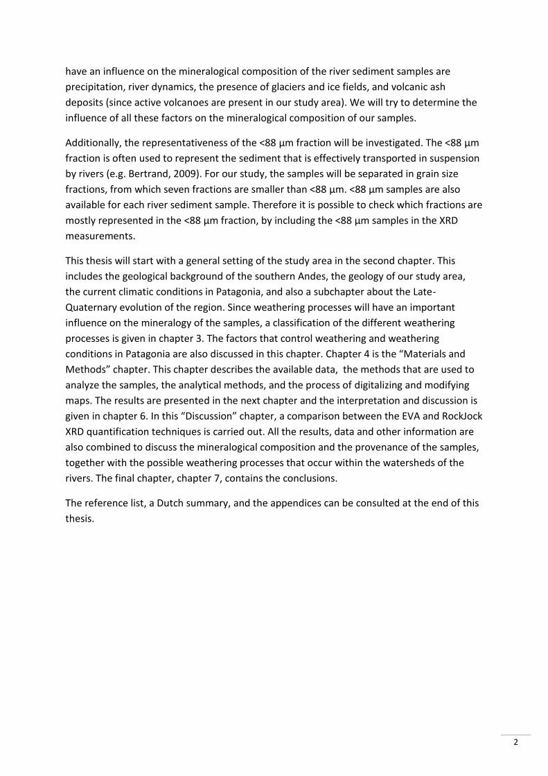
Patagonia is the southernmost region of South America, shared by Chile and Argentina,
which extends from latitude 37° to 56° south and from longitude 65° to 78° west (Fig. 2.1). It
is one of Earth’s most remote areas with a population of less than 2 people per square
kilometer.
The morphology of Patagonia is mostly dominated by the presence of the Patagonian
Cordillera, which is the southern segment of the Andean Cordillera. This mountain chain
divides Patagonia into two morphologically different regions. To the west there is the
fragmentated Chilean mountainous coast dominated by a complex landscape of fjords and
islands. The eastern side consists of the “pampa” of Argentina, flat lands with a dry climate
covered with steppe-like vegetation.
Fig. 2.1. Map of Patagonia (Garreaud et al., 2013).
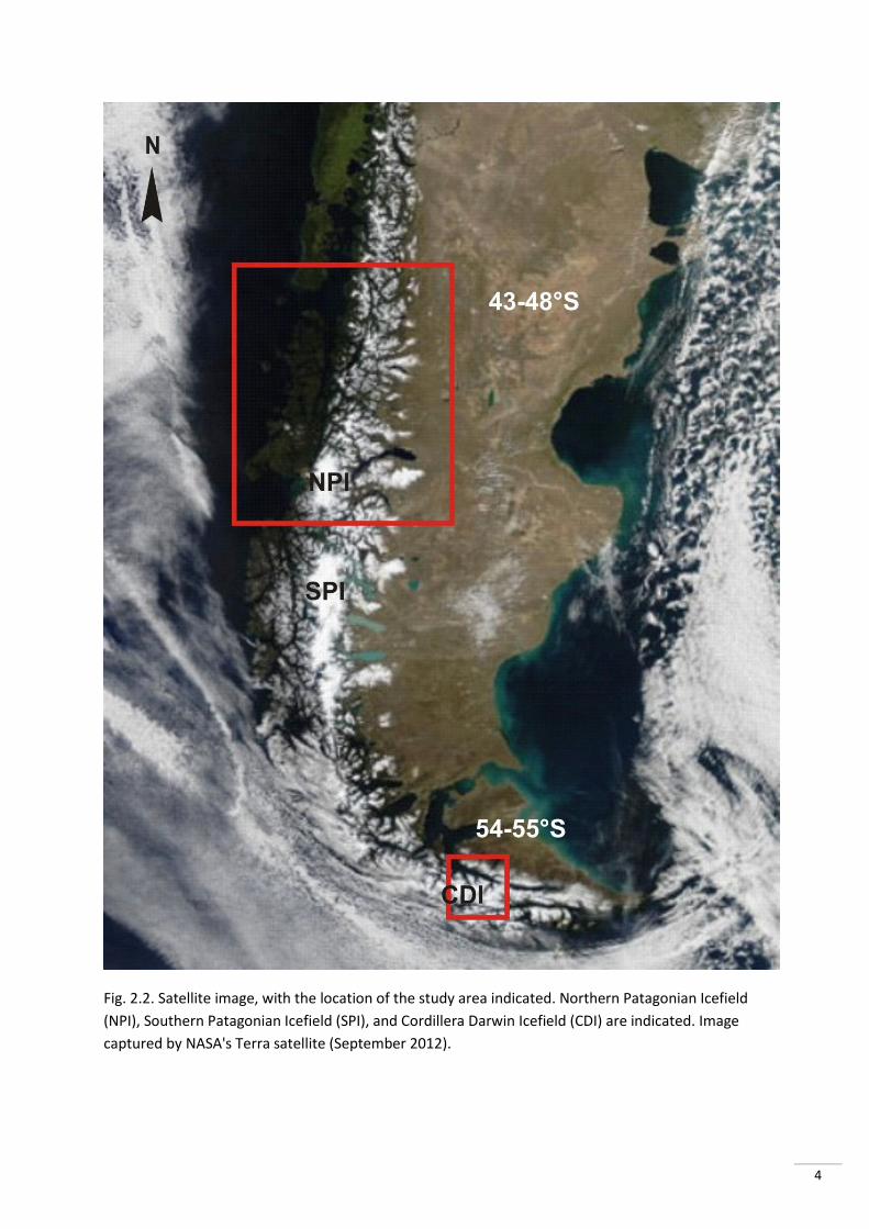
Our main study area, shown in Fig.2.2, is located in Northern Chilean Patagonia between 43°
and 48° S. It includes the Northern Patagonian Icefield in its southern part (Fig 2.2). The
second study area of this thesis lies in the southernmost part of Patagonia, and includes part
of the Cordillera Darwin Icefield (69–70°W and 54–55°S).
4
Fig. 2.2. Satellite image, with the location of the study area indicated. Northern Patagonian Icefield
(NPI), Southern Patagonian Icefield (SPI), and Cordillera Darwin Icefield (CDI) are indicated. Image
captured by NASA's Terra satellite (September 2012).
5
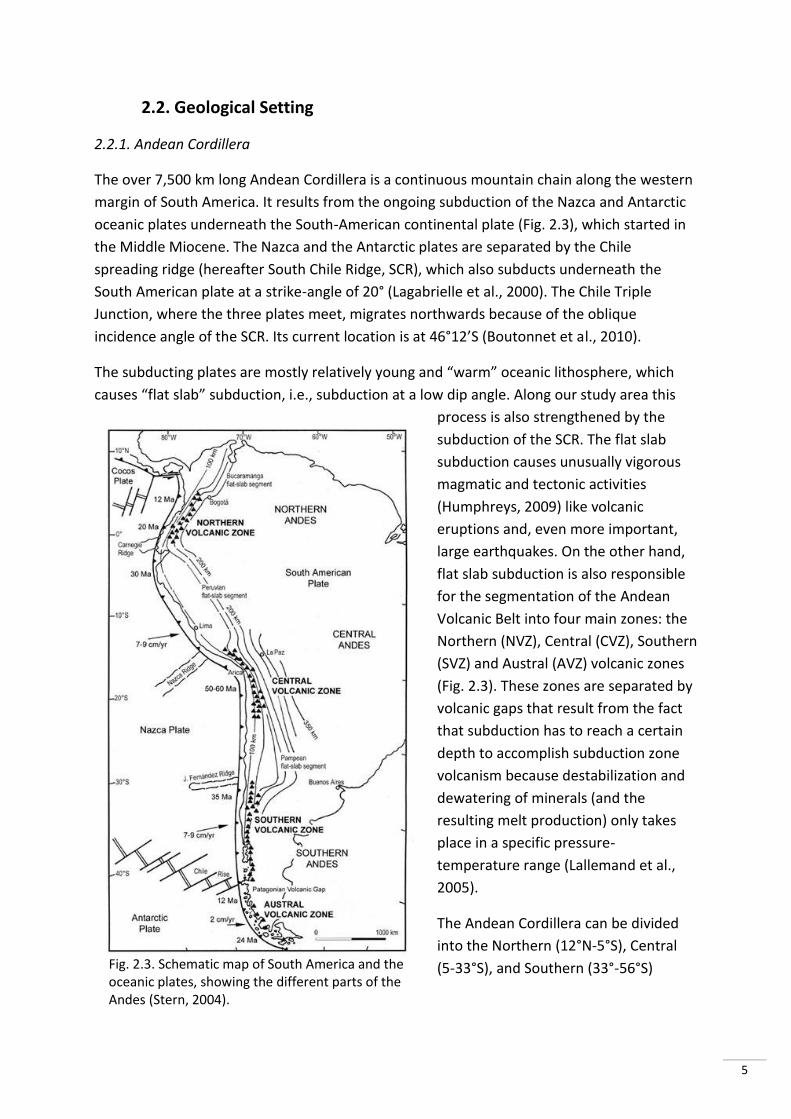
Fig. 2.3. Schematic map of South America and the oceanic plates, showing the different parts of the Andes (Stern, 2004).
2.2. Geological Setting
2.2.1. Andean Cordillera
The over 7,500 km long Andean Cordillera is a continuous mountain chain along the western
margin of South America. It results from the ongoing subduction of the Nazca and Antarctic
oceanic plates underneath the South-American continental plate (Fig. 2.3), which started in
the Middle Miocene. The Nazca and the Antarctic plates are separated by the Chile
spreading ridge (hereafter South Chile Ridge, SCR), which also subducts underneath the
South American plate at a strike-angle of 20° (Lagabrielle et al., 2000). The Chile Triple
Junction, where the three plates meet, migrates northwards because of the oblique
incidence angle of the SCR. Its current location is at 46°12’S (Boutonnet et al., 2010).
The subducting plates are mostly relatively young and “warm” oceanic lithosphere, which
causes “flat slab” subduction, i.e., subduction at a low dip angle. Along our study area this
process is also strengthened by the
subduction of the SCR. The flat slab
subduction causes unusually vigorous
magmatic and tectonic activities
(Humphreys, 2009) like volcanic
eruptions and, even more important,
large earthquakes. On the other hand,
flat slab subduction is also responsible
for the segmentation of the Andean
Volcanic Belt into four main zones: the
Northern (NVZ), Central (CVZ), Southern
(SVZ) and Austral (AVZ) volcanic zones
(Fig. 2.3). These zones are separated by
volcanic gaps that result from the fact
that subduction has to reach a certain
depth to accomplish subduction zone
volcanism because destabilization and
dewatering of minerals (and the
resulting melt production) only takes
place in a specific pressure-
temperature range (Lallemand et al.,
2005).
The Andean Cordillera can be divided
into the Northern (12°N-5°S), Central
(5-33°S), and Southern (33°-56°S)
6
Andes (Fig. 2.3, Stern, 2004). This distinction is based on distinct pre-Andean basement ages,
Mesozoic and Cenozoic geological evolution, crustal thickness, structural trends, active
tectonics and volcanism. The Northern Andes, situated in Colombia and Equador, have a
northeast-southwest trend. The Central Andes are subdivided into the northwest-southeast
trending Peruvian segment called the Northern Central Andes, and the north-south trending
Southern Central Andes in Chile and Argentina. The Southern Andes have a general north-
south trend and part of this segment is located in Patagonia.
2.2.2. Geology of Patagonia
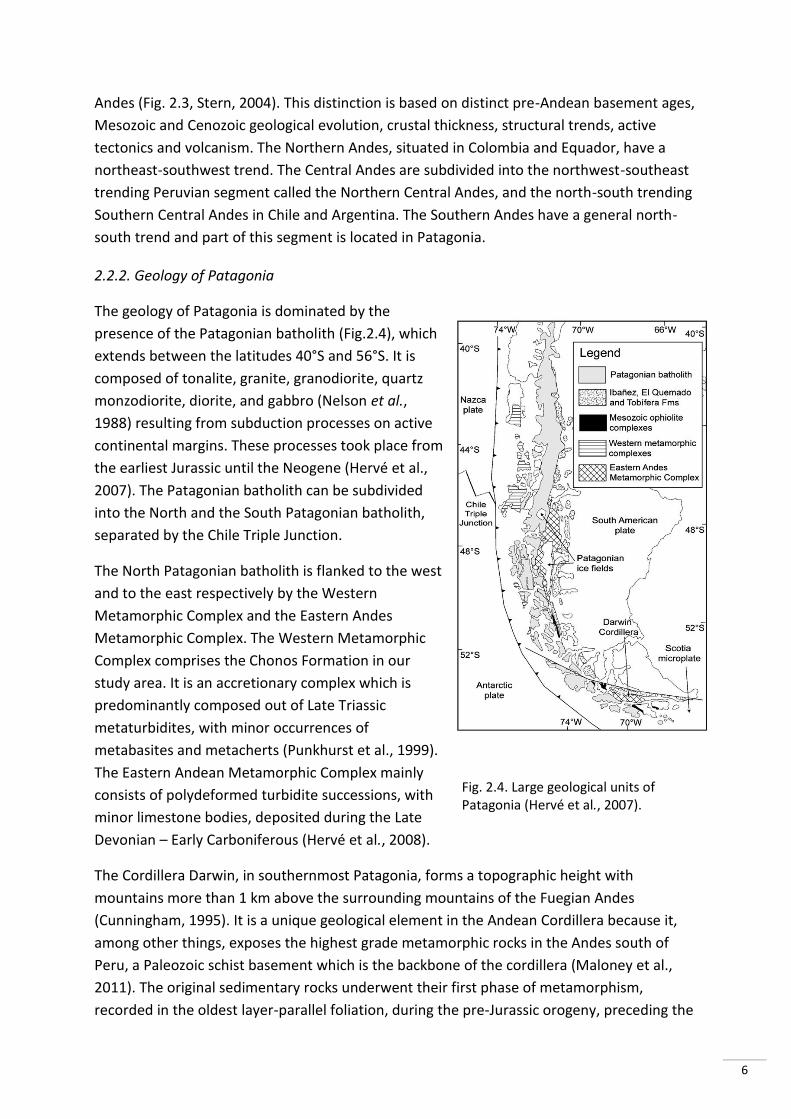
The geology of Patagonia is dominated by the
presence of the Patagonian batholith (Fig.2.4), which
extends between the latitudes 40°S and 56°S. It is
composed of tonalite, granite, granodiorite, quartz
monzodiorite, diorite, and gabbro (Nelson et al.,
1988) resulting from subduction processes on active
continental margins. These processes took place from
the earliest Jurassic until the Neogene (Hervé et al.,
2007). The Patagonian batholith can be subdivided
into the North and the South Patagonian batholith,
separated by the Chile Triple Junction.
The North Patagonian batholith is flanked to the west
and to the east respectively by the Western
Metamorphic Complex and the Eastern Andes
Metamorphic Complex. The Western Metamorphic
Complex comprises the Chonos Formation in our
study area. It is an accretionary complex which is
predominantly composed out of Late Triassic
metaturbidites, with minor occurrences of
metabasites and metacherts (Punkhurst et al., 1999).
The Eastern Andean Metamorphic Complex mainly
consists of polydeformed turbidite successions, with
minor limestone bodies, deposited during the Late
Devonian – Early Carboniferous (Hervé et al., 2008).
The Cordillera Darwin, in southernmost Patagonia, forms a topographic height with
mountains more than 1 km above the surrounding mountains of the Fuegian Andes
(Cunningham, 1995). It is a unique geological element in the Andean Cordillera because it,
among other things, exposes the highest grade metamorphic rocks in the Andes south of
Peru, a Paleozoic schist basement which is the backbone of the cordillera (Maloney et al.,
2011). The original sedimentary rocks underwent their first phase of metamorphism,
recorded in the oldest layer-parallel foliation, during the pre-Jurassic orogeny, preceding the
Fig. 2.4. Large geological units of Patagonia (Hervé et al., 2007).
7
emergence of the Andean mountain chain. At the southern side of the Paleozoic basement a
metamorph felsic ortogneiss, from a 160 Ma intrusive protolite, is present. Both
metamorphic rocks are part of the Eastern Andes Metamorphic Complex (Fig. 2.4), which is
also present in our northern study area. This complex is, around Cordillera Darwin, intruded
by granite suites and mafic dykes and surrounded by mid-Jurassic and younger volcanic rocks
(Maloney et al., 2011). Mesozoic to Cenozoic marine sedimentary rocks complete the
geological substrate picture of our southern study area.
2.2.3. Soils
The soils in Chilean Patagonia are, in very general terms, deep and moist soils, with a rich
and well developed A horizon. This is in contrast with the superficial, often alkaline with an
elevated amount of salt, soils on the Argentine side (Gut, 2008). These moist, wet soils are
susceptible to be degraded through compaction and erosion. The erosional processes are
particularly active because of the hilly landscape and the elevated rate of rainfall that
washes out the organic matter (Ellies, 2000).
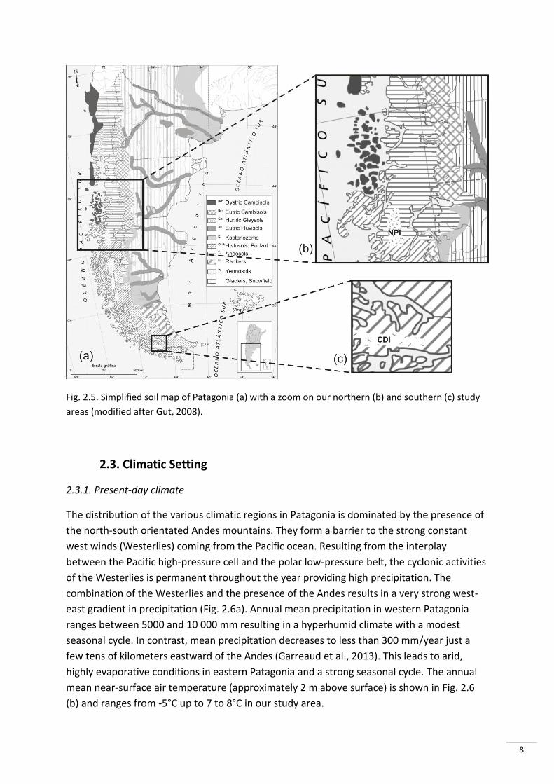
Fig. 2.5 shows a simplified overview of the soil types in southern South America with the 2
study areas enlarged. The following review of the soil types is based on the description of
Gut (2008). The most common soil type in the northern area (Fig. 2.5b) is andosol, i.e., soil
developed on volcanic ashes. These are acid soils with a very high rate of phosphate fixation.
They occur mostly on the steep slopes in the volcanic Andes since they develop on volcanic
deposits or tephra. Dystric cambisols, i.e., poor, acid soils that develop in mountainous
areas, are present on the northwestern side of the study area (the Coastal Range). These
soils develop in mountainous areas with humid climate with a base saturation of less than
50% and little biological activity. They have no phosphate and carbonates are absent in the
parental material. They are highly susceptible to water erosion. At the border with Argentina
eutric cambisols, i.e., neutral soils in subhumid to semiarid zones of transition, occur. These
soils have a base saturation of more than 50% and are biologically active. Carbonates are
also absent in the parental material. The southwestern part of the northern study area
comprises histosols, i.e., peaty, organic soils with 40 cm or more organic material. In the
region, these soils are constantly swept by salt-laden winds so they are low in fertility.
In the southern study area (Fig. 2.5c) only podzols are present. These acid, poor soils are
common in areas with high pluviosity and are highly susceptible to eluviation of iron and
other weathering products. This leaves a bleached, ashy upper horizon and often a dark
colored B horizon.
8
Fig. 2.5. Simplified soil map of Patagonia (a) with a zoom on our northern (b) and southern (c) study
areas (modified after Gut, 2008).
2.3. Climatic Setting
2.3.1. Present-day climate
The distribution of the various climatic regions in Patagonia is dominated by the presence of
the north-south orientated Andes mountains. They form a barrier to the strong constant
west winds (Westerlies) coming from the Pacific ocean. Resulting from the interplay
between the Pacific high-pressure cell and the polar low-pressure belt, the cyclonic activities
of the Westerlies is permanent throughout the year providing high precipitation. The
combination of the Westerlies and the presence of the Andes results in a very strong west-
east gradient in precipitation (Fig. 2.6a). Annual mean precipitation in western Patagonia
ranges between 5000 and 10 000 mm resulting in a hyperhumid climate with a modest
seasonal cycle. In contrast, mean precipitation decreases to less than 300 mm/year just a
few tens of kilometers eastward of the Andes (Garreaud et al., 2013). This leads to arid,
highly evaporative conditions in eastern Patagonia and a strong seasonal cycle. The annual
mean near-surface air temperature (approximately 2 m above surface) is shown in Fig. 2.6
(b) and ranges from -5°C up to 7 to 8°C in our study area.

9
Fig. 2.6. (a) Annual mean precipitation; note the logarithmic color scale. (b) Annual mean near-
surface air temperature (after Garreaud et al., 2013)
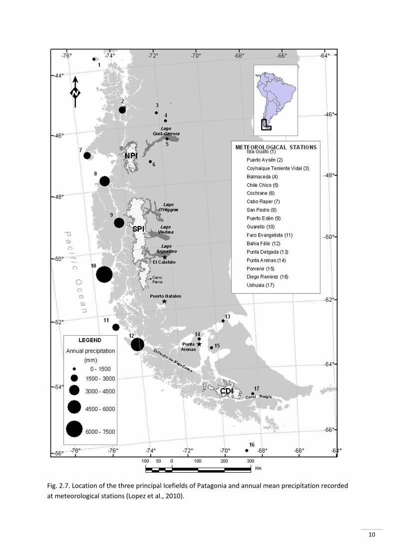
2.3.2. Icefields and their response to climate change
The Northern Patagonian Icefield (NPI), the Southern Patagonian Icefield (SPI), and the
Cordillera Darwin Icefield (CDI) are the three largest temperate ice bodies in the southern
hemisphere (Fig. 2.7). They occupy an area of respectively 4 197 km2, 13 000 km2, and 2 300
km2 (Warren & Sugden, 1993).
The great majority of Patagonian glaciers are temperate glaciers which calve into the Chilean
tidewater fjords to the west and into proglacial freshwater lakes to the east (Warren &
Aniya, 1999). Temperate glaciers are thermally at melting point throughout the year and
they have water present at their base (ice-bedrock contact). Calving glaciers are controlled
by climatic and non-climatic factors. The non-climatic factors comprise the water depth, the
thickness of the ice of the glacier terminus, the geometry of the fjords, bedrock
characteristics, and topography (Lopez et al., 2010). The calving rate is higher when the
water is deeper, the ice is thinner and the topography is steeper.
According to Lopez et al. (2010) the majority of Patagonia’s glaciers have retreated during
the second part of the twentieth century. The NPI and SPI have shrunk considerably in the
last decades, yet a few glaciers in the SPI and CDI remained stable or even advanced.
Rasmussen et al. (2007) even states that the icefields have been losing mass since at least
1870 (i.e., since the Little Ice Age) and that the additional warming of 0.5°C from 1960 to
1999 caused an acceleration in glacier retreat.
10
Fig. 2.7. Location of the three principal Icefields of Patagonia and annual mean precipitation recorded
at meteorological stations (Lopez et al., 2010).
11
The primary control on the recent retreat of glaciers in Patagonia is the increase in air
temperature, but the way in which calving glaciers retreat can be rather complex. When
calving glaciers retreat, periods of substantial abrupt retreats are followed by periods of
stability, in contrast to land-based glacier where there is a linear trend of retreat. As
mentioned above the climatic conditions, which affect the mass and energy balance, partly
determine the rate of retreat, but also the response time of each glacier need to be
considered. The adaptation of a temperate glacier to a mass change can take several years
to several decades, which is still relatively rapid compared to cold glaciers (Lopez et al.,
2010).
Another important climatic factor, which controls glacier mass balance, is precipitation.
Certainly in Patagonia this is probably one of the most important factors for differential
glacier retreats, on which the anomalous behavior of calving glaciers is superimposed
(Warren & Sugden, 1993). While eastern outlets retreated consistently from the beginning
of the 20th century, the retreat of the western glaciers began later, was interrupted by re-
advances, and has accelerated markedly most recently, reaching higher mean rates of
retreat than those in the east. Warren & Sugden (1993) stated that this contrast results from
a dominant temperature control in the east and a predominantly precipitation-controlled
mass-balance regime in the west.
The air temperature, the precipitation control, the response time differences, and the non-
climatic factors controlling calving glaciers together can explain the large differences in the
rate of retreat (and even advance) observed among the Patagonian glaciers.
2.4. Late Quaternary evolution
Several processes such as climate variations, glacial erosion and volcanic activity have
actively transformed the Patagonian landscape during the late Quaternary. These processes
also generated most of the regional superficial deposits, which have an important influence
on the chemical composition of river sediments. These processes and their evolution during
the late Quaternary are therefore reviewed here.
2.4.1 Climate and glacier fluctuations
The Quaternary of Patagonia is marked by several glaciations, which were preceded by older
glaciations from which the oldest took place between approximately 7 and 5 Ma (latest
Miocene – earliest Pliocene; Lagabrielle et al., 2010). Due to the presence of volcanic flows
interbedded between the glaciogenic deposits, and their availability for absolute dating, the
absolute chronology of the Patagonian glaciations is the best present for the Southern
Hemisphere, apart from Antarctica. The cyclical Quaternary glaciations are controlled by
orbital parameters, being the eccentricity of the Earth’s orbit, the axial tilt (obliquity), and
the equinoctial precession. The Quaternary glaciations which had the highest glacier extend
12
were the Great Patagonian Glaciations (GPG). They developed between 1.168 and 1.016 Ma
(Early Pleistocene; Rabassa et al., 2005). Rabassa & Coronato (2009) stated that the GPG
yielded a continuous mountain ice sheet that extended between 36° and 56° S, roughly 2500
km.
The following sections are mainly based on the review of Glasser et al. (2004).
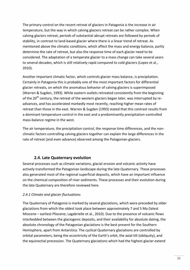
2.4.1.1. Last Glacial Maximum and deglaciation
The Late – Quaternary climate fluctuations can be discussed using the letters A to E for the
Glacial Stages (glacier advances), with A being the oldest and E the youngest. Clapperton
(1993) dated the moraines of Stages B and C between 27,790 and 23,590 yr BP, marking the
Last Glacial Maximum (LGM), while Sugden et al. (2009) date the culminations of Stages B
and C at 23,10025,600 yr and 20,40021,700 yr respectively. The extension of the
Patagonian Ice Sheet (PIS) during the LGM, presented in Fig. 2.8a, has never been greater
from then on. During these stages, the glaciers discharged directly onto outwash planes
occupying the Strait of Magellan, which was then above sea level (Sugden et al., 2009).
Glacial Stage D represents the youngest moraine system at the LGM, and culminated before
17,700 yr BP (Sugden et al., 2009). The glaciers were less extensive then at their maxima at
Stages B and C and terminated in lakes (Fig. 2.8b).
Fig. 2.8. Glacier reconstructions during stages B & C (a), D (b), and E (c), based on field evidence at
five glacier basins between latitudes 47°54° S. Corrections for the eustatic sea level during each
Stage have been applied. (Sugden et al., 2009).
Deglaciation from the LGM limits (17.5 ka) was extremely rapid (Sugden et al., 2005). A
possible explanation for this rapid deglaciation is that the lake levels where higher than at
present, facilitating the retreat of the ice margins. At the western side of the NPI, McCulloch
et al. (2000) associated the ice retreat with stepped warming, indicated by the type of
vegetations that rapidly colonized the exposed land surfaces at that time. This stepped
warming could also (partly) explain the extremely rapid deglaciation.
13
The post – LGM deglaciation was interrupted by glacier advance between 11,700 and 15,500
yr BP. This is Glacial Stage E, which corresponds to the Antarctic Cold Reversal. Unlike the
large ice sheets present during the previous stages, Stage E was characterized by the
presence of three ice sheets (Fig.2.8c; Sugden et al., 2009), which were the onset for what
we now call the North Patagonian Icefield, the South Patagonian Icefield, and the Cordillera
Darwin ice field.
After Glacial Stage E, a second step in deglaciation occurred (11.4 ka; Sugden et al., 2005).
This warming, and an increase in precipitation, allowed the invasion of forests in the
mountain foothills and fjord sites in the Magellan area, replacing the steppe tundra
vegetation (McCulloch at al., 2000). This second step in deglaciation is seen as the onset of
the Holocene in southernmost South America.
2.4.1.2. Holocene
Temperature and precipitation have fluctuated considerably during the Holocene to the east
of the Andes. Between 10,000 and 8000 14C years BP the climate improved, with increasing
summer temperatures and decreasing precipitation. From 8000 to 6000 14C years BP
temperature continued to increase, but also precipitation increased. The period between
6000 and 3600 14C years BP appears to have been colder and wetter than present, followed
by an arid phase until 3000 14C years BP. From 3000 14C years BP to the present day, there is
evidence of a cold phase, with relatively high precipitation.
West of the Andes, evidence points to periods of drier than present conditions between
94006300 14C years BP and 24001600 14C years BP. Climate amelioration was present
between 10,300 and 8550 14C years BP. Afterwards there was an increase in precipitation,
followed by an arid period around 5000 14C years BP. After 5000 14C years BP evidence points
to a cooler and wetter climate. This cooling trend was interrupted twice, at around 3000 and
350 14C years BP, until present, with temperatures higher than present. The maxima in the
precipitation record roughly correspond with the temperature minima, with the highest
values between 4950 and 3160 14C years BP, followed by another peak sometime between
3160 and 800 14C years BP, and a final peak between 350 14C years BP and present.
The established Holocene chronology for glacier fluctuations in the Patagonian Andes is
based on radiocarbon dates for moraines in front of the outlet glaciers (e.g. Mercer, 1982).
Based on these dates Mercer proposed three Neoglacial advances since 5000 14C years BP,
the first at 47004200 14C years BP, the second at 27002000 14C years BP, and the third
during the Little Ice Age of the last three centuries. The first one in thought to be the
greatest, with moraines located ~15 km in front of the modern ice-front of outlet glaciers of
the northwest side of the NPI. Glasser et al. (2004) observed an advance of the Soler glacier
between AD 1220 and AD 1340. These dates are comparable to recorded advances of four
other southern Patagonian glaciers. This was a period when there was a poleward shift in
precipitation and winter precipitation was above the long term mean (Villalba, 1994). This
14
highlights the importance of precipitation on glaciers advances, which may have been more
important than changes in atmospheric temperature.
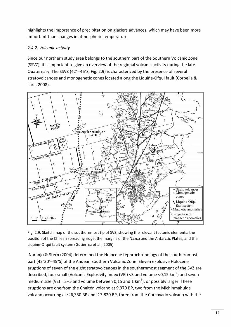
2.4.2. Volcanic activity
Since our northern study area belongs to the southern part of the Southern Volcanic Zone
(SSVZ), it is important to give an overview of the regional volcanic activity during the late
Quaternary. The SSVZ (42°46°S, Fig. 2.9) is characterized by the presence of several
stratovolcanoes and monogenetic cones located along the Liquiñe-Ofqui fault (Corbella &
Lara, 2008).
Fig. 2.9. Sketch map of the southernmost tip of SVZ, showing the relevant tectonic elements: the
position of the Chilean spreading ridge, the margins of the Nazca and the Antarctic Plates, and the
Liquine-Ofqui fault system (Gutiérrez et al., 2005).
Naranjo & Stern (2004) determined the Holocene tephrochronology of the southernmost
part (42°30’45°S) of the Andean Southern Volcanic Zone. Eleven explosive Holocene
eruptions of seven of the eight stratovolcanoes in the southernmost segment of the SVZ are
described, four small (Volcanic Explosivity Index (VEI) <3 and volume <0,15 km3) and seven
medium size (VEI = 35 and volume between 0,15 and 1 km3), or possibly larger. These
eruptions are one from the Chaitén volcano at 9,370 BP, two from the Michinmahuida
volcano occurring at 6,350 BP and 3,820 BP, three from the Corcovado volcano with the
15
oldest one occurring sometime between 9,190 and 7,980 BP and two younger ones at
7,980 BP and 6,870 BP, one from the Yanteles volcano at 9,190 and two form the
Melimoyu volcano occurring at 2,740 BP and 1,750 BP, one from the Mentolat volcano at
6,960 BP, and one from the Macá volcano at 1,540 BP. The total amount of eleven
eruptions occurring in 8000 years implies a frequency of one eruption approximately every
725 years in this segment of the SVZ. In contrast, the Hudson volcano, the most southern
(and largest) volcano in our northern study area, has had three very large and nine other
documented small explosive Holocene eruptions, and thus both larger and more explosive
Holocene eruptions than all the other centres in the SSVZ combined. The Hudson volcano, a
large ice-filled caldera complex, is thought to be so active because of its vicinity to the Chile
triple junction (Naranjo & Stern, 2004). The two large prehistoric explosive eruptions
occurred at approximately 6700 BP and 4800 BP (Naranjo & Stern, 1998).
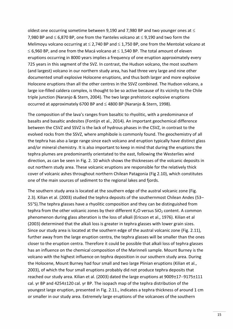
The composition of the lava’s ranges from basaltic to rhyolitic, with a predominance of
basalts and basaltic andesites (Fontijn et al., 2014). An important geochemical difference
between the CSVZ and SSVZ is the lack of hydrous phases in the CSVZ, in contrast to the
evolved rocks from the SSVZ, where amphibole is commonly found. The geochemistry of all
the tephra has also a large range since each volcano and eruption typically have distinct glass
and/or mineral chemistry. It is also important to keep in mind that during the eruptions the
tephra plumes are predominantly orientated to the east, following the Westerlies wind
direction, as can be seen in Fig. 2. 10 which shows the thicknesses of the volcanic deposits in
out northern study area. These volcanic eruptions are responsible for the relatively thick
cover of volcanic ashes throughout northern Chilean Patagonia (Fig 2.10), which constitutes
one of the main sources of sediment to the regional lakes and fjords.
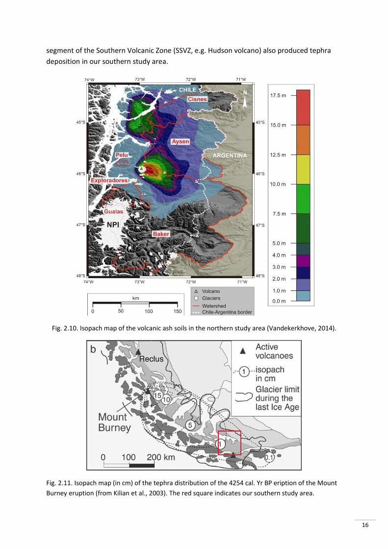
The southern study area is located at the southern edge of the austral volcanic zone (Fig.
2.3). Kilian et al. (2003) studied the tephra deposits of the southernmost Chilean Andes (53–
55°S).The tephra glasses have a rhyolitic composition and they can be distinguished from
tephra from the other volcanic zones by their different K2O versus SiO2 content. A common
phenomenon during glass alteration is the loss of alkali (Ericson et al., 1976). Kilian et al
(2003) determined that the alkali loss is greater in tephra glasses with lower grain sizes.
Since our study area is located at the southern edge of the austral volcanic zone (Fig. 2.11),
further away from the large eruption centra, the tephra glasses will be smaller than the ones
closer to the eruption centra. Therefore it could be possible that alkali loss of tephra glasses
has an influence on the chemical composition of the Marinneli sample. Mount Burney is the
volcano with the highest influence on tephra deposition in our southern study area. During
the Holocene, Mount Burney had four small and two large Plinian eruptions (Kilian et al.,
2003), of which the four small eruptions probably did not produce tephra deposits that
reached our study area. Kilian et al. (2003) dated the large eruptions at 9009±179175±111
cal. yr BP and 4254±120 cal. yr BP. The isopach map of the tephra distribution of the
youngest large eruption, presented in Fig. 2.11., indicates a tephra thickness of around 1 cm
or smaller in our study area. Extremely large eruptions of the volcanoes of the southern
16
segment of the Southern Volcanic Zone (SSVZ, e.g. Hudson volcano) also produced tephra
deposition in our southern study area.
Fig. 2.10. Isopach map of the volcanic ash soils in the northern study area (Vandekerkhove, 2014).
Fig. 2.11. Isopach map (in cm) of the tephra distribution of the 4254 cal. Yr BP eription of the Mount
Burney eruption (from Kilian et al., 2003). The red square indicates our southern study area.
17
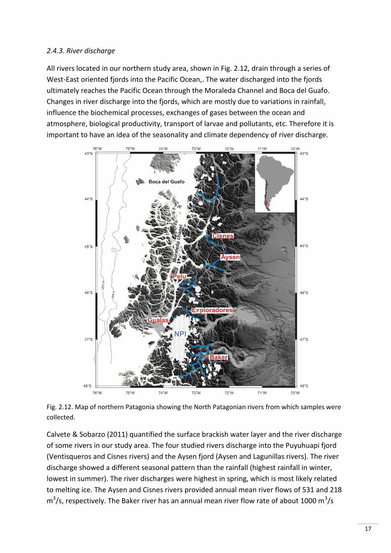
2.4.3. River discharge
All rivers located in our northern study area, shown in Fig. 2.12, drain through a series of
West-East oriented fjords into the Pacific Ocean,. The water discharged into the fjords
ultimately reaches the Pacific Ocean through the Moraleda Channel and Boca del Guafo.
Changes in river discharge into the fjords, which are mostly due to variations in rainfall,
influence the biochemical processes, exchanges of gases between the ocean and
atmosphere, biological productivity, transport of larvae and pollutants, etc. Therefore it is
important to have an idea of the seasonality and climate dependency of river discharge.
Fig. 2.12. Map of northern Patagonia showing the North Patagonian rivers from which samples were
collected.
Calvete & Sobarzo (2011) quantified the surface brackish water layer and the river discharge
of some rivers in our study area. The four studied rivers discharge into the Puyuhuapi fjord
(Ventisqueros and Cisnes rivers) and the Aysen fjord (Aysen and Lagunillas rivers). The river
discharge showed a different seasonal pattern than the rainfall (highest rainfall in winter,
lowest in summer). The river discharges were highest in spring, which is most likely related
to melting ice. The Aysen and Cisnes rivers provided annual mean river flows of 531 and 218
m3/s, respectively. The Baker river has an annual mean river flow rate of about 1000 m3/s
18
(Quiroga et al., 2012) but with a very strong seasonality, reflecting the periods of maximum
(summer) and minimum (spring) ice melt. The Pelu river drains a steep, mountainous area
that receives a high year-round precipitation. Since the glacier coverage of the watershed is
less than 2 %, river discharge is mostly controlled by rainfall (Bertrand et al., 2014). The
Exploradores river and the Gualas river both spring at large glaciers from the NPI, so a strong
seasonality in river discharge and a high influence of glacier melt water is expected. The
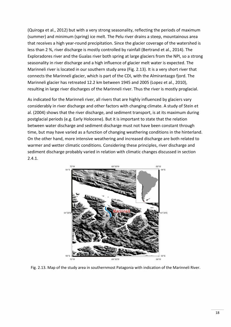
Marinneli river is located in our southern study area (Fig. 2.13). It is a very short river that
connects the Marinneli glacier, which is part of the CDI, with the Almirantazgo fjord. The
Marinneli glacier has retreated 12.2 km between 1945 and 2005 (Lopez et al., 2010),
resulting in large river discharges of the Marinneli river. Thus the river is mostly proglacial.
As indicated for the Marinneli river, all rivers that are highly influenced by glaciers vary
considerably in river discharge and other factors with changing climate. A study of Stein et
al. (2004) shows that the river discharge, and sediment transport, is at its maximum during
postglacial periods (e.g. Early Holocene). But it is important to state that the relation
between water discharge and sediment discharge must not have been constant through
time, but may have varied as a function of changing weathering conditions in the hinterland.
On the other hand, more intensive weathering and increased discharge are both related to
warmer and wetter climatic conditions. Considering these principles, river discharge and
sediment discharge probably varied in relation with climatic changes discussed in section
2.4.1.
Fig. 2.13. Map of the study area in southernmost Patagonia with indication of the Marinneli River.
19
3. Weathering Processes
3.1. Introduction
River sediment is the product of weathering and erosion. Most rivers integrate different
lithologies, climates and soil types so the composition of river sediments depends on the
multiple weathering processes that occur in their watershed. Therefore it is important to
discuss the weathering and erosional processes, together with their relation to the climate,
lithologies, and soils of Patagonia.
In general, the weathering processes can be subdivided into physical (mechanical), chemical,
and biological. A generally accepted view is that physical weathering predominantly occurs
in very cold and/or very dry environments, while chemical weathering is dominant in regions
with a wet and hot climate. But, like Hall et al. (2002) stated, weathering in cold
environments might be less physically dominated than previously thought since it is shown
that chemical weathering is not always temperature-limited but is rather limited by moisture
availability. Chemical and physical weathering often go hand in hand, e.g. physical abrasion
decreases the particle size, which consequently results in increasing the surface area, making
them more susceptible for chemical weathering.
The following classification is made according to the book “Weathering and the Riverine
Denudation of Continents” (Depetris et al., 2014).
3.2. Physical Weathering
Physical weathering is the process by which rocks are broken down into smaller pieces,
without changing their chemical composition. It is the process that breaks the rock structure.
Once the particles start moving it is called erosion. The high impact physical weathering
processes are driven by the drastic physical power of water, ice, wind, pressure and
temperature change.
3.2.1. Frost Weathering
Frost weathering includes the physical weathering processes that are water-based and occur
at low temperatures, being freeze-thaw weathering, hydration shattering, ice crystal growth,
and hydraulic pressure.
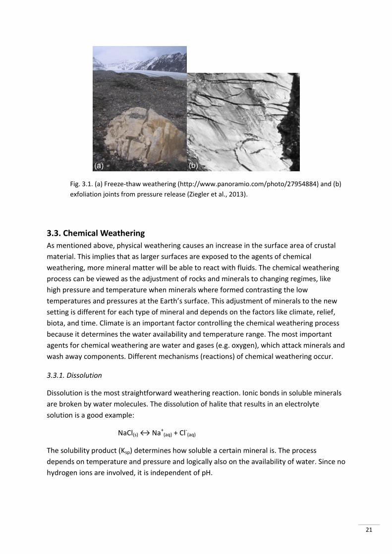
Freeze-thaw weathering (Fig. 3.1a), as the name indicates, results from the successive
freezing and thawing of water inside the rocks. The freeze-thaw process begins when water
enters fissures in bare rocks. During freezing nights the water freezes and expands, causing
the rock to break. When the ice melts again, more room is present for additional water to
enter the rock, more ice can be formed during freezing nights and the process continues.
Important factors influencing the effectiveness of the freeze-thaw process are rock
properties (pore size, permeability, etc.), temperature regime, and moisture availability.
Freeze-thaw weathering is thought to be a significant process of landform development in
20
mountainous regions and high latitudes. The resulting clasts of the process are generally
angular. A remarkable result of laboratory tests showed that over 100 freeze and thaw
cycles, quartz was fractured preferentially over feldspar (Schwamborn et al., 2012).
3.2.2. Salt Weathering
Salt weathering is caused by the formation or expansion of salts. They can be formed from
the reaction between acids and bases or from the expansion of already existing crystals by
heating or hydration. The expanding salts exert a pressure on the pore-walls of the rock. The
supply of salt can comes from rising ground water, wind-blown dust, sea water infiltration,
or atmospheric pollution. Since this process mainly occurs in arid areas (deserts) it will not
be further discussed because it is unlikely to take place in our study area.
3.2.3. Insolation Weathering
Insolation weathering, or thermal stress, results from the expansion and contraction of rock
caused by changes in temperature (insolation of the sun). Cracking of the rocks occurs when
the stresses build up by expansion or contraction exceed the rock’s elastic limit. This process
is most effective in regions where received solar radiation is high and where temperatures
differences between day and night are very distinct. Since this is not the case for Patagonia
(a lot of cloud cover, rainfall, and high wind speeds), insolation weathering will not be an
important process for our research.
3.2.4. Pressure-Release Weathering
When rocks, subjected to a high confining pressure from overlying materials, get exhumed
due to removal of the overlying material they may expand and fracture parallel to the
surface, producing sheet or dilatational joints (Fig. 3.1b). The originally overlying material
can be rocks (that get eroded) or ice. Thus, pressure-release weathering can be more
common during periods of glacial retreat and possibly be an indicator for warmer periods.
Granitic rocks are known to be susceptible for the formation of these joint sets parallel to
the local land surface, when exhumed (e.g. Ziegler et al., 2013). The presence of the
Patagonian icesheets and the Patagonian batholith may cause this type of weathering to be
important.
3.2.5. Wetting and Drying
This weathering process is based on the adsorption of water molecules as successive layers
inside fractured rocks. It occurs when the polar water molecules are attracted to the walls of
a fine crack. Successive cycles of wetting and drying will cause expansion and contraction
because the swelling pressure of water addition to the crack may be followed by attraction
during dry periods when residual water molecules on opposing faces of the crack are pulled
together.
21
Fig. 3.1. (a) Freeze-thaw weathering (http://www.panoramio.com/photo/27954884) and (b)
exfoliation joints from pressure release (Ziegler et al., 2013).
3.3. Chemical Weathering
As mentioned above, physical weathering causes an increase in the surface area of crustal
material. This implies that as larger surfaces are exposed to the agents of chemical
weathering, more mineral matter will be able to react with fluids. The chemical weathering
process can be viewed as the adjustment of rocks and minerals to changing regimes, like
high pressure and temperature when minerals where formed contrasting the low
temperatures and pressures at the Earth’s surface. This adjustment of minerals to the new
setting is different for each type of mineral and depends on the factors like climate, relief,
biota, and time. Climate is an important factor controlling the chemical weathering process
because it determines the water availability and temperature range. The most important
agents for chemical weathering are water and gases (e.g. oxygen), which attack minerals and
wash away components. Different mechanisms (reactions) of chemical weathering occur.
3.3.1. Dissolution
Dissolution is the most straightforward weathering reaction. Ionic bonds in soluble minerals
are broken by water molecules. The dissolution of halite that results in an electrolyte
solution is a good example:
NaCl(s) ↔ Na+(aq) + Cl-(aq)
The solubility product (Ksp) determines how soluble a certain mineral is. The process
depends on temperature and pressure and logically also on the availability of water. Since no
hydrogen ions are involved, it is independent of pH.
22
3.3.2. Hydration
The hydration process involves the attachment of H+ and OH- ions to the atoms and
molecules of a mineral, i.e. the absorption of water. When the minerals take up water, the
increased volume creates physical stresses within the rock, which weakens the rock
structure. A common example is the hydration of anhydrite to gypsum:
CaSO4 + 2 H2O ↔ CaSO4.2H2O
3.3.3. Carbonation
Carbonation is probably the most common geochemical mechanism. It results from the
weathering effects of CO2 in aqueous solution (as H2CO3) and the interaction with CaCO3,
which may give rise to spectacular karst landscapes. The pH of water is influenced by the
presence of CO2, the more CO2, the lower the pH (the more acidic). Water in equilibrium
with the atmosphere has a pH of ± 5.6 but groundwater may be more acidic because the
concentration of CO2 can be to 30 times higher due to the CO2 production through biological
respiration and the higher partial pressure in soil air. The carbon dioxide can react with
water to form carbonic acid:
CO2(g) + H2O ↔ H2CO3(aq)
The weak carbonic acid can dissociate further:
H2CO3(aq) ↔ H+(aq) + HCO3
-(aq)
This bicarbonate ion itself can than dissociate also:
HCO3-(aq) ↔ H+
(aq) + CO3-(aq)
These last two equations clearly show the pH dependency of the reactions. Limestone gets
dissolved by water which contains dissolved CO2 (or carbonic acid) by following reaction:
CaCO3 + H2O + CO2(aq) ↔ Ca2+(aq) + 2 HCO3
-(aq)
This dissolution is responsible for the creation of caves and other karst features in calcareous
terrains. Carbonation is a mechanism that exports alkalinity from the continents to the sea.
If the equilibrium of the reaction is shifted towards the left (often in the oceans), carbonates
can be formed and CO2 returns to the gaseous pool.
3.3.4. Hydrolysis
Hydrolysis implies the chemical reaction or breaking down of a chemical compound, such as
a silicate. It may occur under neutral, acidic, or basic conditions were cations give rise to
weak bases and/or anions give rise to weak acids. A typical acid hydrolysis, which is a very
common weathering process, is the incongruent dissolution of sodium feldspar to clay by
CO2-saturated water:
23
2 NaAlSi3O8(s) + 9 H2O + 2 H2CO3(aq) ↔ Al2Si2O5(OH)4(s) + 2 Na+(aq) + 2 HCO3
-(aq) + 4 H4SiO4(aq)
In theory, this reaction is not spontaneous and a large quantity of carbonic acid is needed for
the reaction to occur. In practice the aqueous solutions move away from the mineral surface
and are rapidly replaced by a significant amount of fresh carbonated water coming into
contact with the mineral surface. Hydrolysis of silicates is of very high significance in the
overall picture of continental chemical weathering.
3.3.5. Oxidation-Reduction (Redox) Processes
Redox reactions are common weathering reaction in aqueous solutions. Reduction and
oxidation occur together but in weathering processes one product may be more relevant
than the others. Usually free oxygen (i.e., dissolved in water) is the oxidizing agent in
oxidation reactions. A good example is the rusting of iron:
4 FeO(s) + O2(g) → 2 Fe2O3(s)
The equilibrium constant is in the order of 1042, indicating that the reaction will go practically
to completion. Sulphides are also quite susceptible to oxidation. The oxidation of pyrite for
example generates sulphuric acid (H2SO4). The resulting acidity subsequently enhances the
solubility of other metals like aluminium so dissolution and chemical denudation are
enhanced.
Reduction is less significant in weathering processes than oxidation. Organic matter typically
operates as a reducing agent. Organic debris or tissue are oxidized to form CO2 or to form
new organic compounds. SO42- can be reduced by microbes which use the oxygen in the
sulphate to oxidize organic matter. The resulting sulphide can react with H+ to enter the gas
pool, or it can react with metals to precipitate (e.g., pyrite).
3.3.6. Exchangeable Ions
Fine-grained weathering products of minerals can act as a source of exchangeable cations
and anions which may be involved in supplementary weathering processes. These clays and
colloids carry many negative charges on their surface and positive exchangeable ions
attached to the surface. Anion exchange is rather rare in comparison with cation exchange
(H+, Na+, Ca2+, Al3+, etc.). The Cation Exchange Capacity (CEC) of a particle can be defined as
the concentration of cations in milliequivalents per 100 g of soil or sediment. The adsorbed
cations can have an effect on the chemical composition of the soil solution, so they may
affect other weathering processes.
3.4. Biological Weathering
Biological activity can cause both physical and chemical weathering. Significant biological
agents in mineral and rock breakdown are roots, lichens, algae, mosses, fungi, and bacteria.
Microorganisms can produce aggressive substances, like organic acids, that dissolve minerals
24
and produce secondary phases. Organisms can either apply physical stress or they may
produce substances, which gives rise to the subdivision between biophysical weathering and
biochemical weathering.
3.4.1. Biophysical Weathering
Biophysical weathering is dominated by the activities of roots. Roots may exert physical
pressure and they can also provide a pathway for water infiltration. However, there is still an
ongoing discussion about the mechanical role of roots, some authors have demonstrated
that cracks and holes in minerals, which were mistakenly attributed to the action of roots,
were actually produced by chemical dissolution mechanisms (Sverdrup, 2009). Others argue
that the effect of roots is far from efficient and only sufficient to fracture some weak rocks.
Lichens, composite organisms of fungi and algae, are also capable of physically breaking
rocks by penetration and by increasing their water content. The significance of weathering
by lichens and algae is substantial in extremely cold environments, like Antarctica.
3.4.2. Biochemical Weathering
In the rhizosphere (soils zones dominated by roots) roots can enhance the weathering
process. In addition to mechanical weathering, they can also cause chemical weathering by
emitting and absorbing components. The tip of the root can release organic acids, together
with protons and electrons, which contribute to mineral decay through delivery and
mobilization of iron and aluminium.
Lichens can also, after their stage of physical weathering, cause chemical weathering due to
the excretion of organic acids. Hereby extensive rock surface corrosion occurs. The
effectiveness of lichens, which is often studied on granites, is also high on different rock
types, and it is higher in extreme (cold and dry) environments (Hall et al., 2005). Hall et al.
(2005) evidenced that the assumed freeze-thaw weathering on the Qinghai-Tibet Plateau
was in fact attributable to the action of lichens.
Fungi are significant drivers or organic matter decomposition in forest ecosystems. Mineral
soils of boreal forests are often intensively colonized by fungi, so in these regions weathering
by fungi can have an important role.
The last discussed organisms causing chemical weathering, are uni- or multicellular
microscopic organisms which have colonized the Earth for over three billion years, bacteria.
The mechanisms used by bacteria to weather minerals are redox reactions, dissolution
reactions, and the production of weathering agents, such as protons, organic acids, and
chelating molecules. Bacteria can cause a lowering of the pH of soil solutions (to 4 or 5) by
respiration, oxygen consumption and carbon dioxide production, which has a major impact
on the chemical weathering of minerals.
25
Evidence for bacterial activity in glacial meltwater is given by Scharp et al. (1999). They
stated that (1) microbially mediated redox reactions may be important at glacier beds, (2)
chemical weathering in glacial environments not only arises from purely inorganic reactions,
and (3) redox reactions could be the major proton source beneath ice sheets where
meltwaters are isolated from an atmospheric source of CO2.
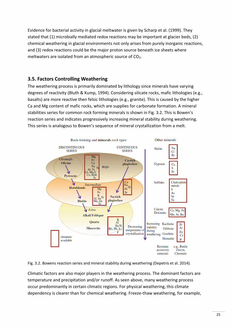
3.5. Factors Controlling Weathering
The weathering process is primarily dominated by lithology since minerals have varying
degrees of reactivity (Bluth & Kump, 1994). Considering silicate rocks, mafic lithologies (e.g.,
basalts) are more reactive then felsic lithologies (e.g., granite). This is caused by the higher
Ca and Mg content of mafic rocks, which are supplies for carbonate formation. A mineral
stabilities series for common rock forming minerals is shown in Fig. 3.2. This is Bowen’s
reaction series and indicates progressively increasing mineral stability during weathering.
This series is analogous to Bowen’s sequence of mineral crystallization from a melt.
Fig. 3.2. Bowens reaction series and mineral stability during weathering (Depetris et al. 2014).
Climatic factors are also major players in the weathering process. The dominant factors are
temperature and precipitation and/or runoff. As seen above, many weathering process
occur predominantly in certain climatic regions. For physical weathering, this climate
dependency is clearer than for chemical weathering. Freeze-thaw weathering, for example,
26
requires a specific temperature range (around the freezing point) and water must be
available. West et al. (2005) investigated the climatic controls on silicate weathering. They
stated that it is hard to distinguish the temperature sensitivity of silicate weathering rates
from other factors. Nevertheless, weathering of silicates is enhanced with increasing
temperature and precipitation.
Erosion rate, together with temperature and precipitation, completes the top three factors
controlling silicate weathering for a given rock type. Erosion rates are important since they
determine the mineral supply and the available mineral surface for weathering.
Another controlling factor is acidity. Acidity is mostly supplied from atmospheric CO2, either
as organic acids produced by vegetation or in soil waters, and it is the driving force for the
dissolution reaction. Since acidity can be vegetation dependant, and vegetation is in close
relationship with temperature and precipitation, acidity is also influenced by climatic
changes (Kelly et al., 1998).
The effect of soil cover can also be of major importance (Oliva et al., 2003). Weathering can
be strongly influenced by the hydrological and physical properties of a soil-covered system.
Thick soils can isolate parent material from weathering. Considering the soil-influence on
weathering, vegetation can have contradictory effects. On the one hand, vegetation protects
the soil form physical erosion, enhancing the development of thick soils. But on the other
hand, the low pH environment close to the root system and the presence of organic acids
resulting from plant biodegradation should enhance mineral dissolution.
3.6. Weathering in Patagonia
Since weathering processes strongly depend on the lithology of the bedrock and on the
nature of the soils, an overview of weathering conditions for the common lithologies in our
study area is given. Studies on weathering processes in Patagonia are relatively scarce. A
study on weathering in South Patagonian rivers was done by Lee et al. (2013), but the focus
of their study lies more on the rivers in eastern Patagonia (Argentina). An interesting
conclusion of their study is that weathering of sedimentary volcanic material contributes
significantly to the dissolved loads in the rivers.
3.6.1. Bedrock
The North Patagonian batholith occupies a large area in our northern study area. As seen in
section 2.2.2, the lithology is dominantly granitic (tonalite, granite, granodiorite, quartz
monzodiorite, diorite, and gabbro). The lithology of the intrusive plutons in our southern
study area also granitic. Granite mainly consists in quartz, plagioclase, alkali feldspar, and
micas. Quartz is vey resistant to weathering and therefore it mostly stays unaltered when
eroded. Feldspars are easily weathered and transformed into e.g., kaolinite by chemical
weathering. Apart from feldspars, also amphiboles, epidote and apatite are easily weathered
27
(Oliva et al., 2003). A positive correlation between temperature and element fluxes, silica in
particular, from weathering is determined by White & Blum (1995). French & Guglielmin
(2000) investigated granitic weathering in Antarctica and stated that in cryogenic
environments the susceptibility of quartz to be fractured is enhanced.
The Eastern Andean Metamorphic Complex (EAMC), which is present in both study areas, is
the second large unit in our study area. It is composed of metasedimentary rocks
(metasandstone, metapelite-schist, metaconglomerate, metachert, metaturbitite, and
marbles; Ramírez-Sánchez et.al., 2005). The dominant minerals present in the EAMC,
detected using XRD by Ramírez-Sánchez et al. (2005), are quartz, albite, muscovite, and
chlorite. Muscovite is highly resistant to weathering. In contrast, albite (and other
plagioclase) will weather quite rapidly which results in the formation of clay minerals such as
smectite and kaolinite (Harris, 1995). It is noteworthy that alkali feldspar weather more
slowly than plagioclase because weathering of silicates preferentially attacks Na- and Ca-rich
phases.
Finally, our study region in Northern Chilean Patagonia also contains significant amounts of
Quaternary volcanic rocks. Weathering of volcanic rocks is described by Pola et al. (2012).
They determined a high preferential removal of Ca and Na by the dissolution of plagioclase.
At a higher degree of alteration, also mobile oxides (Al2O3, Fe2O3, CaO, Na2O, K2O) are highly
removed from the rock.
3.6.2. Soils
Large parts of the bedrock in Northern Chilean Patagonia are covered by soils. These soils
also have a high influence on the nature of river sediments. Therefore it is useful to discuss
the mineralogy and geochemistry of the soils.
The most common type of soils in the study area is andosols, i.e., soils developed on volcanic
ashes. These soils contain high proportions of volcanic glass and amorphous colloidal
materials, like allophone, imogolite, and ferrihydrite. Dissolution of the glass can occur,
resulting in Si and Al leaching out of the soils. However, Sigfusson et al. (2006) stated that
the dissolution rates of the basaltic glass (and probably also allophone and imogolite) are
slowed down by lower temperatures. The neutral to basic eutric cambisols are formed by
the dissolution and removal of carbonates, alteration of primary minerals such as mica and
feldspar, and the formation of silicate clay and precipitation of iron-hydroxides. Since no
carbonates are present in the Patagonian eutric cambisols (Gut, 2008), they were either
removed by dissolution, or they were not present in the bedrock material. Histosols consist
predominantly out of organic matter. Their possible influence on river sediments is
consequently also of organic kind. Podzols are present in our southern study area. They are
highly susceptible to eluviation of iron and other weathering products, leaving an acidic,
poor horizon.
28
4. Material & Methods
4.1. Samples and data obtained prior to this study
4.1.1. River sediment samples
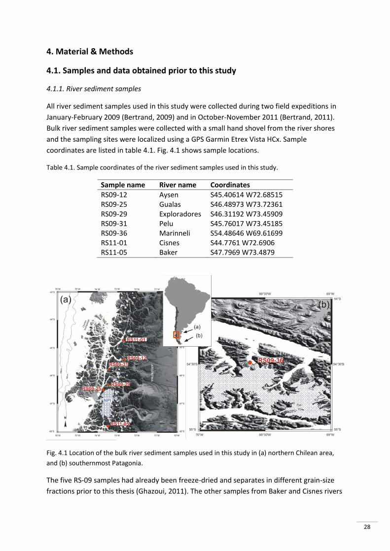
All river sediment samples used in this study were collected during two field expeditions in
January-February 2009 (Bertrand, 2009) and in October-November 2011 (Bertrand, 2011).
Bulk river sediment samples were collected with a small hand shovel from the river shores
and the sampling sites were localized using a GPS Garmin Etrex Vista HCx. Sample
coordinates are listed in table 4.1. Fig. 4.1 shows sample locations.
Table 4.1. Sample coordinates of the river sediment samples used in this study.
Sample name River name Coordinates
RS09-12 Aysen S45.40614 W72.68515 RS09-25 Gualas S46.48973 W73.72361 RS09-29 Exploradores S46.31192 W73.45909 RS09-31 Pelu S45.76017 W73.45185 RS09-36 Marinneli S54.48646 W69.61699 RS11-01 Cisnes S44.7761 W72.6906 RS11-05 Baker S47.7969 W73.4879
Fig. 4.1 Location of the bulk river sediment samples used in this study in (a) northern Chilean area,
and (b) southernmost Patagonia.
The five RS-09 samples had already been freeze-dried and separates in different grain-size
fractions prior to this thesis (Ghazoui, 2011). The other samples from Baker and Cisnes rivers
29
(RS11-01 and RS11-05) were entirely prepared for this thesis, as explained below (section
4.2)
4.1.2. Geochemical Data
The elemental geochemical composition of the different grain-size fractions of the five RS-09
samples was measured prior to the start of this thesis. The geochemical analyses were
performed at the Woods Hole Oceanographic Institution, MA, USA, using Inductively
Coupled Plasma Atomic Emission Spectrometry (ICP-AES). Analytical details are presented in
Bertrand et al. (2012). The data is presented in Appendix A.
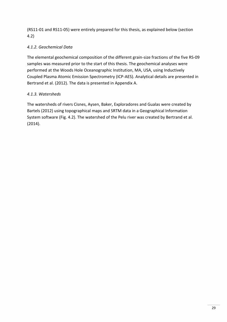
4.1.3. Watersheds
The watersheds of rivers Cisnes, Aysen, Baker, Exploradores and Gualas were created by
Bartels (2012) using topographical maps and SRTM data in a Geographical Information
System software (Fig. 4.2). The watershed of the Pelu river was created by Bertrand et al.
(2014).
30
Fig. 4.2. Watersheds of rivers Cisnes, Aysen, Baker, Exploradores, Gualas, and Pelu (Bartels, 2012).
4.2. Sediment sample preparation
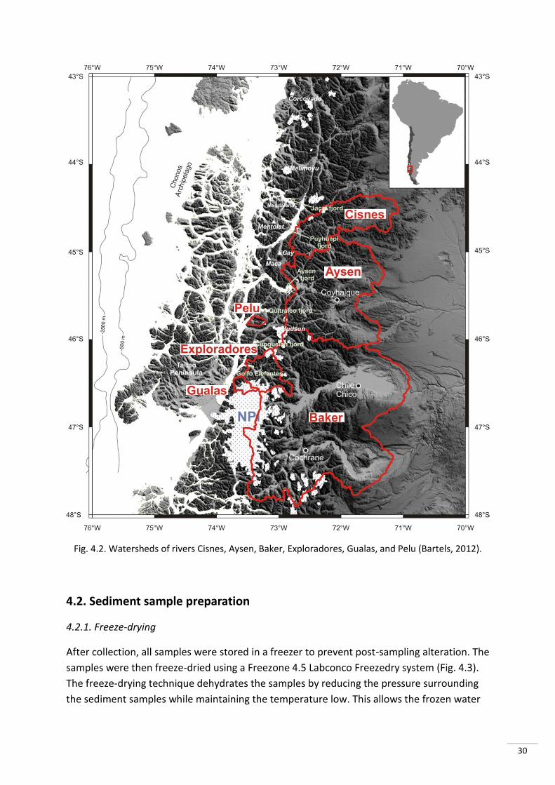
4.2.1. Freeze-drying
After collection, all samples were stored in a freezer to prevent post-sampling alteration. The
samples were then freeze-dried using a Freezone 4.5 Labconco Freezedry system (Fig. 4.3).
The freeze-drying technique dehydrates the samples by reducing the pressure surrounding
the sediment samples while maintaining the temperature low. This allows the frozen water
31
in the material to sublimate directly from the solid phase to the gas phase. Freeze-drying is
generally more time-consuming than oven-drying but the main advantage is that the
physical structure of the sample does not change when removing the water (Loring &
Rantalle, 1992).
The freeze-drier uses an Edwards vacuum pump to place the chamber containing the
samples under vacuum. Because of the low pressure and low temperature (approximately -
40°C) the frozen pore water starts to sublimate. Then the water vapor gets re-deposited on
the coiling inside the condensing chamber, positioned underneath the sample chamber. This
process needs to run for several days for all the pore water to be removed, leaving only solid
particles in the sample.
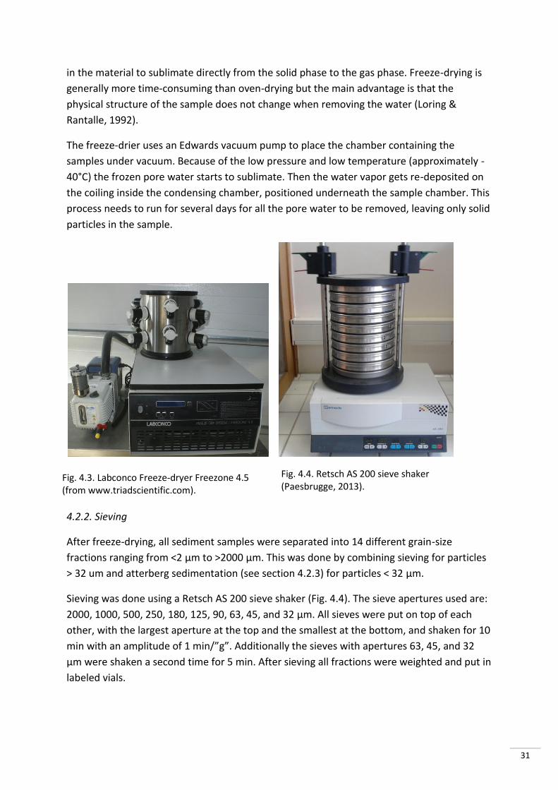
4.2.2. Sieving
After freeze-drying, all sediment samples were separated into 14 different grain-size
fractions ranging from <2 µm to >2000 µm. This was done by combining sieving for particles
> 32 um and atterberg sedimentation (see section 4.2.3) for particles < 32 µm.
Sieving was done using a Retsch AS 200 sieve shaker (Fig. 4.4). The sieve apertures used are:
2000, 1000, 500, 250, 180, 125, 90, 63, 45, and 32 µm. All sieves were put on top of each
other, with the largest aperture at the top and the smallest at the bottom, and shaken for 10
min with an amplitude of 1 min/”g”. Additionally the sieves with apertures 63, 45, and 32
µm were shaken a second time for 5 min. After sieving all fractions were weighted and put in
labeled vials.
Fig. 4.3. Labconco Freeze-dryer Freezone 4.5 (from www.triadscientific.com).
Fig. 4.4. Retsch AS 200 sieve shaker (Paesbrugge, 2013).
32
4.2.3. Atterberg Column
To separate the particles smaller than 32 µm into the fractions <2, 2 – 4, 4 – 8, 8 – 16, and 16
– 32 µm the method of the Atterberg - Stokes Column was used. This method is based on
the differential settling time of particles with different particle diameter. The Stoke’s
Formula (4.1) is used to calculate the settling time of a particle with a certain radius in a
water-filled column over a certain height.
(4.1)
Settling times were calculated for a height of 30 cm. Values for the density of the falling
sphere, and density and viscosity of the liquid were taken from Müller & Schmicke (1967).
Since the viscosity of water (η) is temperature dependant, a set of settling times were
calculated for common room temperatures. To make sure the water was at room
temperature, a plastic barrel was filled with distilled water at least one day before using it.
Once the measurements were carried out, room temperature was corresponding and the
right settling time was used.
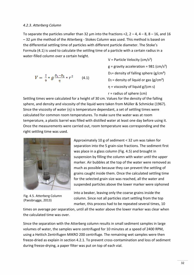
Approximately 10 g of sediment < 32 um was taken for
separation into the 5 grain-size fractions. The sediment first
was place in a glass column (Fig. 4.5) and brought in
suspension by filling the column with water until the upper
marker. Air bubbles at the top of the water were removed as
much as possible because they can prevent the settling of
grains caught inside them. Once the calculated settling time
for the selected grain size was reached, all the water and
suspended particles above the lower marker were siphoned
into a beaker, leaving only the coarse grains inside the
column. Since not all particles start settling from the top
marker, this process had to be repeated several times, 10
times on average per separation, until all the water above the lower marker was clear when
the calculated time was over.
Since the separation with the Atterberg column results in small sediment samples in large
volumes of water, the samples were centrifuged for 10 minutes at a speed of 2400 RPM,
using a Hettich Zentrifugen MIKRO 200 centrifuge. The remaining wet samples were then
freeze-dried as explain in section 4.2.1. To prevent cross-contamination and loss of sediment
during freeze-drying, a paper filter was put on top of each vial.
V = Particle Velocity (cm/s²)
g = gravity acceleration = 981 (cm/s²)
D1= density of falling sphere (g/cm³)
D2 = density of liquid or gas (g/cm³)
η = viscosity of liquid g/(cm s)
r = radius of sphere (cm)
Fig. 4.5. Atterberg Column (Paesbrugge, 2013)
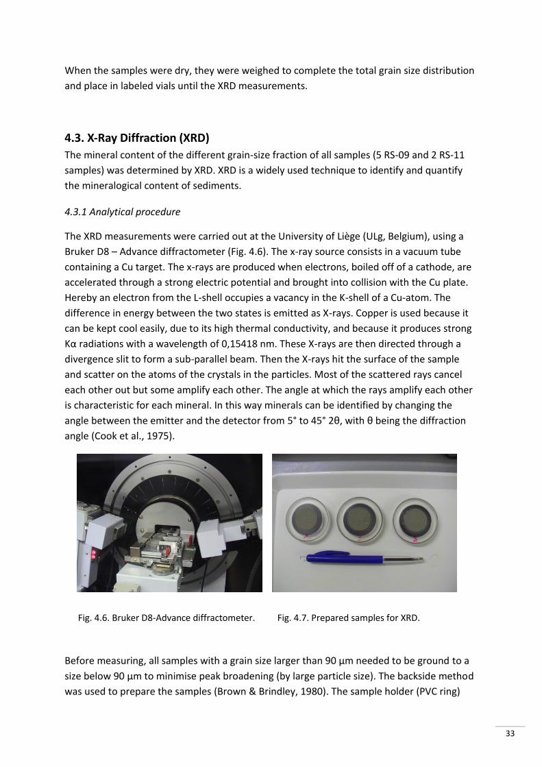
33
When the samples were dry, they were weighed to complete the total grain size distribution
and place in labeled vials until the XRD measurements.
4.3. X-Ray Diffraction (XRD)
The mineral content of the different grain-size fraction of all samples (5 RS-09 and 2 RS-11
samples) was determined by XRD. XRD is a widely used technique to identify and quantify
the mineralogical content of sediments.
4.3.1 Analytical procedure
The XRD measurements were carried out at the University of Liège (ULg, Belgium), using a
Bruker D8 – Advance diffractometer (Fig. 4.6). The x-ray source consists in a vacuum tube
containing a Cu target. The x-rays are produced when electrons, boiled off of a cathode, are
accelerated through a strong electric potential and brought into collision with the Cu plate.
Hereby an electron from the L-shell occupies a vacancy in the K-shell of a Cu-atom. The
difference in energy between the two states is emitted as X-rays. Copper is used because it
can be kept cool easily, due to its high thermal conductivity, and because it produces strong
Kα radiations with a wavelength of 0,15418 nm. These X-rays are then directed through a
divergence slit to form a sub-parallel beam. Then the X-rays hit the surface of the sample
and scatter on the atoms of the crystals in the particles. Most of the scattered rays cancel
each other out but some amplify each other. The angle at which the rays amplify each other
is characteristic for each mineral. In this way minerals can be identified by changing the
angle between the emitter and the detector from 5° to 45° 2θ, with θ being the diffraction
angle (Cook et al., 1975).
Before measuring, all samples with a grain size larger than 90 µm needed to be ground to a
size below 90 µm to minimise peak broadening (by large particle size). The backside method
was used to prepare the samples (Brown & Brindley, 1980). The sample holder (PVC ring)
Fig. 4.7. Prepared samples for XRD. Fig. 4.6. Bruker D8-Advance diffractometer.

34
was positioned on a ground glass plate (to prevent preferential orientation of the grains),
filled with sediment, closed off with a lid, and then turned around. The surface of the
sediment should then be nicely even and ready for analysis (Fig. 4.7).
The diffraction angle was set to vary between 5° and 45° 2θ with a step size of 0,02° 2θ. This
requires a measuring time of approximately one hour per sample but the outcome is a high
resolution diffractogram.
4.3.2. Semi-quantification using EVA
The identification and the semi-quantification of the mineral assemblages of the obtained
XRD scans was done using the Bruker – EVA software program. Each peak or a set of peaks
results from the diffraction of a specific mineral. The minerals commonly identified in the
diffractograms are listed in table 4.2.
For each raw diffractogram (Fig. 4.8a), the background noise is subtracted (Background set
at 0), and the spectra is smoothed (Smooth set at 0,1) using the EVA software. If needed, the
diffractograms are then centered using the peak position of quartz can be done (principal
peak at 3,34 Å) since the peak position of quartz is always fixed (quartz has always the same
chemical composition). A good mineral identification requires that every peak is accounted
for by principal and secondary peaks of the chosen minerals. A database in the EVA software
from which minerals can be selected allows a fast, easy, and reliable identification of the
minerals present (Fig. 4.8b). For each mineral the intensity of the principal peak can be
adjusted. While doing so the intensities of the secondary peaks also automatically adapts,
which allows you to examine whether a certain peak is only a secondary peak of one mineral
or if it is possibly an accumulation of two peaks, caused by different minerals, on top of each
other. Once all minerals are identified, the maximum counts (intensities) of all principal
peaks are measured. Not all minerals generate a diffraction peak as high and well defined as
quartz, therefore the counts from a primary peak of a certain mineral are multiplied by its
correction factor (Table 4.2). Correction factors are taken from Cook et al. (1975). After
multiplying the counts with the corresponding correction factors a relative quantification of
the minerals can be obtained.
Table 4.2. Theoretical d-value of principal peaks of common minerals and their correction factors
(after Cook et al., 1975).
Mineral Principal peak (Å) Correction Factor
Quartz 3.34 1.00 Plagioclase (Albite) 3.21 – 3.16 2.80
K – feldspar (Orthoclase) 3.26 – 3.21 4.30 Pyroxene (Augite) 3.00 – 2.99 5.00
Amphibole (Hornblende) 8.59 – 8.27 2.50 Olivine (Forsterite) 2.45 5.00 Total clay content 4.50 – 4.47 20.00
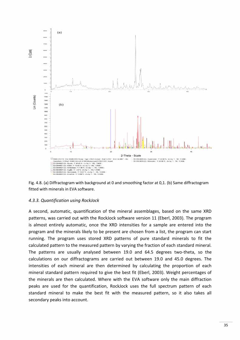
35
Fig. 4.8. (a) Diffractogram with background at 0 and smoothing factor at 0,1. (b) Same diffractogram
fitted with minerals in EVA software.
4.3.3. Quantification using RockJock
A second, automatic, quantification of the mineral assemblages, based on the same XRD
patterns, was carried out with the RockJock software version 11 (Eberl, 2003). The program
is almost entirely automatic, once the XRD intensities for a sample are entered into the
program and the minerals likely to be present are chosen from a list, the program can start
running. The program uses stored XRD patterns of pure standard minerals to fit the
calculated pattern to the measured pattern by varying the fraction of each standard mineral.
The patterns are usually analysed between 19.0 and 64.5 degrees two-theta, so the
calculations on our diffractograms are carried out between 19.0 and 45.0 degrees. The
intensities of each mineral are then determined by calculating the proportion of each
mineral standard pattern required to give the best fit (Eberl, 2003). Weight percentages of
the minerals are then calculated. Where with the EVA software only the main diffraction
peaks are used for the quantification, RockJock uses the full spectrum pattern of each
standard mineral to make the best fit with the measured pattern, so it also takes all
secondary peaks into account.

36
First, the raw files were converted into excel files, using PowDLL Converter. Then, the
patterns were shifted using the main quartz diffraction peak, similarly as with the Eva
software. Although RockJock has an automatic Shifter option, were the choice can be made
to which main peak you want to shift, this feature did not work correctly so all samples were
shifted manually by aligning the main quartz peak with exactly 26.68° 2θ.The intensity data
were then loaded into RockJock and analyzed between 19 and 45 degrees. The main tool to
check whether the quantification is representative or not is the Degree of fit between the
measured and the calculated patterns. The smaller this value is, the better.
The choice of minerals likely to be present is given in Table 4.3. For plagioclase, K-feldspar,
and pyroxene, a range of possible minerals is used since the composition of these minerals
can vary. Common clay minerals were also added. After quantification, all minerals
corresponding to a certain mineral series were grouped into their specific series (plagioclase,
K-feldspar, and pyroxene). All clay minerals were also combined into a “total clay content”
group.
Table 4.3. Selected minerals for the RockJock analysis.
NON - CLAYS CLAYS
Quartz Kaolinite (disordered) K-feldspar (ordered Microcline) Smectite (ferruginous) K-feldspar (intermediate microcline) Illite (1MD) K-feldspar (sanidine) Chlorite (Fe-rich; Tusc) K-feldspar (orthoclase) K-feldspar (anorthoclase) Plagioclase (albite, var. cleavelandite) Plagioclase (oligoclase; NC) Plagioclase (oligoclase; Norway) Plagioclase (andesine) Plagioclase (labradorite) Plagioclase (bytownite) Plagioclase (anorthite) Calcite Pyroxene (augite) Pyroxene (enstatite) Amphibole (hornblende)
37
4.4. Statistical Analysis
Statistical analysis can be very helpful when result are interpreted. It can calculate and
visualize similarities and differences between variables. Results obtained during this study
and available data obtained prior to this study (section 4.1) will be compiled in one large
dataset. Statistical analysis will be carried out in order to facilitate the investigation of
correlations and trends within the dataset.
The dependency between different variables can be calculated by using the Pearson
correlation. The Pearson correlation test creates a correlation matrix. This is a m x m matrix,
with m being the number of variables, that displays the Pearson correlation coefficients (r).
The correlation coefficient is a measure for the strength of the linear coherence between
two variables. A strong positive correlation has a value close to +1, and a strong negative
correlation has a value close to -1. To determine whether the correlation coefficient is
statistically significant or not, a p-value had to calculated. This p-value is the probability of a
test result to be significant or not. The smaller the p-value, the more significant the test
result is. In our statistical analyses a p-value of 0.01 is taken for the significance level. P-
values are largely dependent on the amount of observations. The larger the sample size, the
lower the p-values. Correlations with a corresponding p-value lower than 0.01 will be
considered significant.
The mineralogical and geochemical data were analyzed using Principle Component Analysis
(PCA), which is one of the most frequently used multivariate data analysis methods. It is an
ideal statistical method when working with data sets in which n observations are described
by a large amount of p variables. The main goal of PCA is to reduce the dimensionality of a
data set by replacing the m variables by k principal components, with k being smaller than m
(Jolliffe, 1989). Hereby the maximum amount of information from the initial dimensions is
conserved and accounted for by the minimum amount of principal components.
The program used to carry out the statistical analyses is XLSTAT-Pro, which is a statistical
add-in for Microsoft Excel. The PCA was performed using the Pearson correlation coefficient
as the index of similarity. Using the test significance option, correlations with a significance
level of 0,01 are shown in bold.

38
4.5. Cartography
For the analysis and interpretation of the results the use of geographical software was
needed to organize and present data that could be spatially referenced. A series of maps
was summarized to construct a compiled map for the northern study area and one for the
southern study area.
The data to start from is SRTM (Shuttle Radar Topography Mission) data. It is a three-
dimensional digital terrain model acquired by scanning the Earth’s surface with two satellites
equipped with high resolution altitude meters. The scanning was performed with radar
waves with a resolution of 3 arc-seconds (90 meter). The SRTM data can be downloaded
from the server of the United States Geological Survey
(http://dds.cr.usgs.gov/srtm/version2_1/SRTM1/) in tiles of one by one degrees latitude/
longitude. It is important to use the Version 2 data because this is already processes data
where the water body is leveled and the coast line in defined, unlike Version 1 (Bhang and
Schwartz, 2008). This was necessary because an “ocean” layer (colored ocean and
transparent land) had to be constructed. In total 29 tiles were downloaded for the northern
area (43 – 48°S; 70 – 76°W) and one tile for the southern area (54 – 55°S; 69 – 70°W). The
downloaded tiles were then processed with the SRTMFill program to fill in moderate sized
Null holes (null value areas) by interpolation of the surrounding edges. This ensures that
there are no gaps in the constructed digital elevation model. The SRTM data was imported in
Global Mapper 13 to construct the digital elevation map (Fig. 4.9).
Fig. 4.9. SRTM data of the northern area visualized in Global Mapper 13. (The gap in the upper left
corner is because there is no SRTM data available for the ocean.)
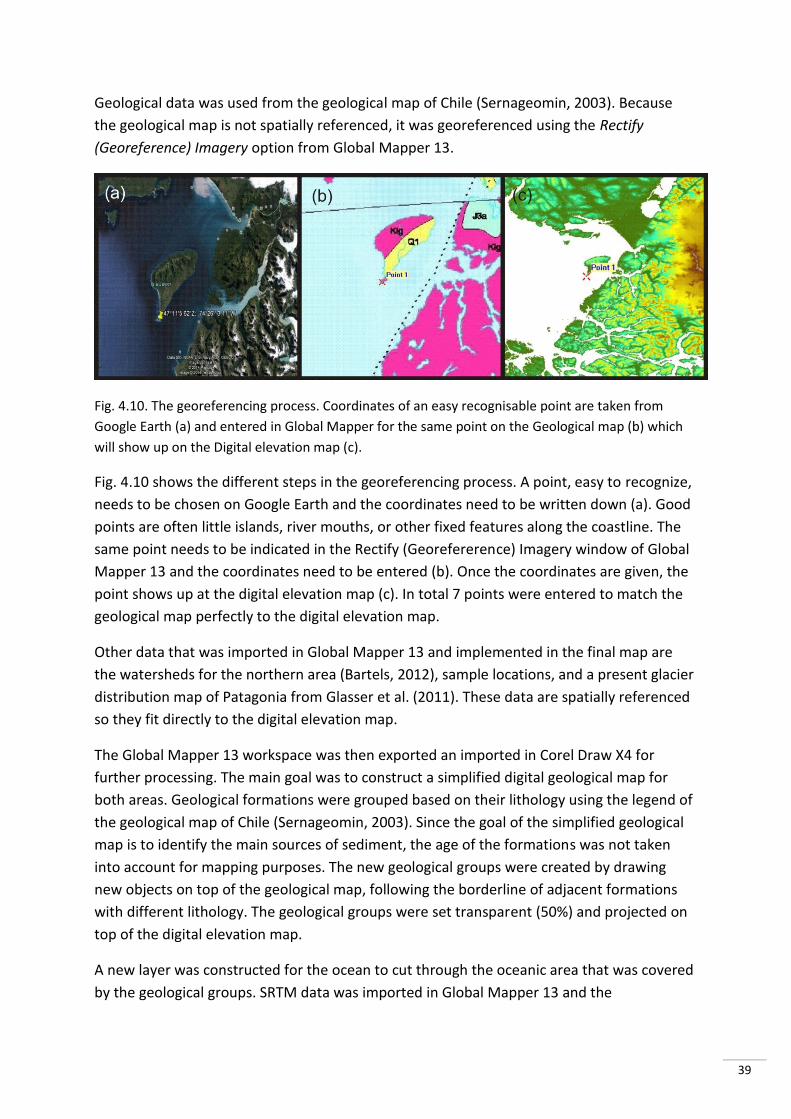
39
Geological data was used from the geological map of Chile (Sernageomin, 2003). Because
the geological map is not spatially referenced, it was georeferenced using the Rectify
(Georeference) Imagery option from Global Mapper 13.
Fig. 4.10. The georeferencing process. Coordinates of an easy recognisable point are taken from
Google Earth (a) and entered in Global Mapper for the same point on the Geological map (b) which
will show up on the Digital elevation map (c).
Fig. 4.10 shows the different steps in the georeferencing process. A point, easy to recognize,
needs to be chosen on Google Earth and the coordinates need to be written down (a). Good
points are often little islands, river mouths, or other fixed features along the coastline. The
same point needs to be indicated in the Rectify (Georefererence) Imagery window of Global
Mapper 13 and the coordinates need to be entered (b). Once the coordinates are given, the
point shows up at the digital elevation map (c). In total 7 points were entered to match the
geological map perfectly to the digital elevation map.
Other data that was imported in Global Mapper 13 and implemented in the final map are
the watersheds for the northern area (Bartels, 2012), sample locations, and a present glacier
distribution map of Patagonia from Glasser et al. (2011). These data are spatially referenced
so they fit directly to the digital elevation map.
The Global Mapper 13 workspace was then exported an imported in Corel Draw X4 for
further processing. The main goal was to construct a simplified digital geological map for
both areas. Geological formations were grouped based on their lithology using the legend of
the geological map of Chile (Sernageomin, 2003). Since the goal of the simplified geological
map is to identify the main sources of sediment, the age of the formations was not taken
into account for mapping purposes. The new geological groups were created by drawing
new objects on top of the geological map, following the borderline of adjacent formations
with different lithology. The geological groups were set transparent (50%) and projected on
top of the digital elevation map.
A new layer was constructed for the ocean to cut through the oceanic area that was covered
by the geological groups. SRTM data was imported in Global Mapper 13 and the
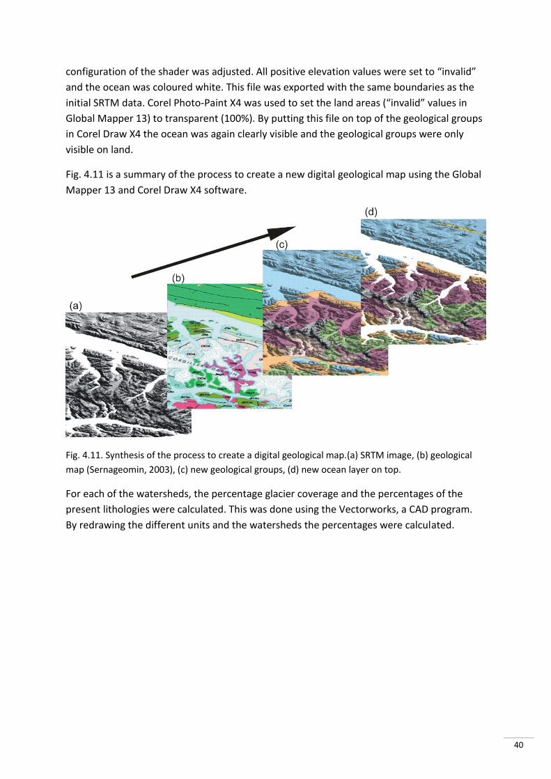
40
configuration of the shader was adjusted. All positive elevation values were set to “invalid”
and the ocean was coloured white. This file was exported with the same boundaries as the
initial SRTM data. Corel Photo-Paint X4 was used to set the land areas (“invalid” values in
Global Mapper 13) to transparent (100%). By putting this file on top of the geological groups
in Corel Draw X4 the ocean was again clearly visible and the geological groups were only
visible on land.
Fig. 4.11 is a summary of the process to create a new digital geological map using the Global
Mapper 13 and Corel Draw X4 software.
Fig. 4.11. Synthesis of the process to create a digital geological map.(a) SRTM image, (b) geological
map (Sernageomin, 2003), (c) new geological groups, (d) new ocean layer on top.
For each of the watersheds, the percentage glacier coverage and the percentages of the
present lithologies were calculated. This was done using the Vectorworks, a CAD program.
By redrawing the different units and the watersheds the percentages were calculated.
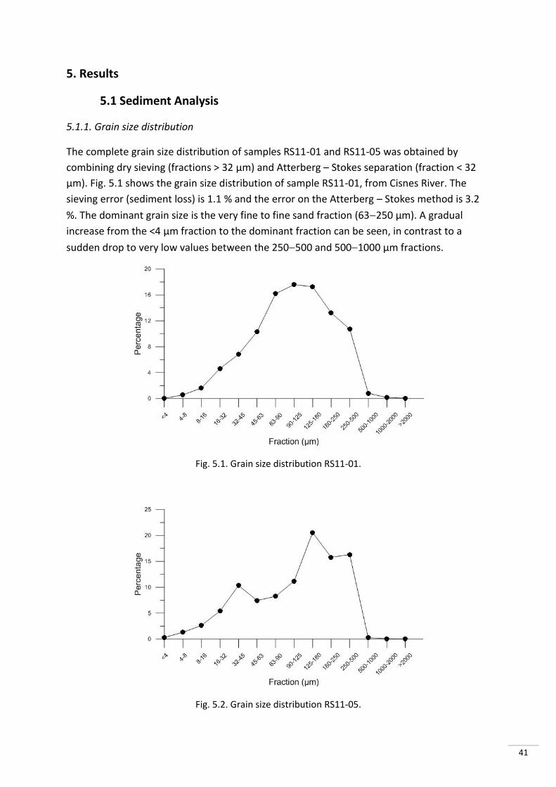
41
5. Results
5.1 Sediment Analysis
5.1.1. Grain size distribution
The complete grain size distribution of samples RS11-01 and RS11-05 was obtained by
combining dry sieving (fractions > 32 µm) and Atterberg – Stokes separation (fraction < 32
µm). Fig. 5.1 shows the grain size distribution of sample RS11-01, from Cisnes River. The
sieving error (sediment loss) is 1.1 % and the error on the Atterberg – Stokes method is 3.2
%. The dominant grain size is the very fine to fine sand fraction (63250 µm). A gradual
increase from the <4 µm fraction to the dominant fraction can be seen, in contrast to a
sudden drop to very low values between the 250500 and 5001000 µm fractions.
Fig. 5.1. Grain size distribution RS11-01.
Fig. 5.2. Grain size distribution RS11-05.
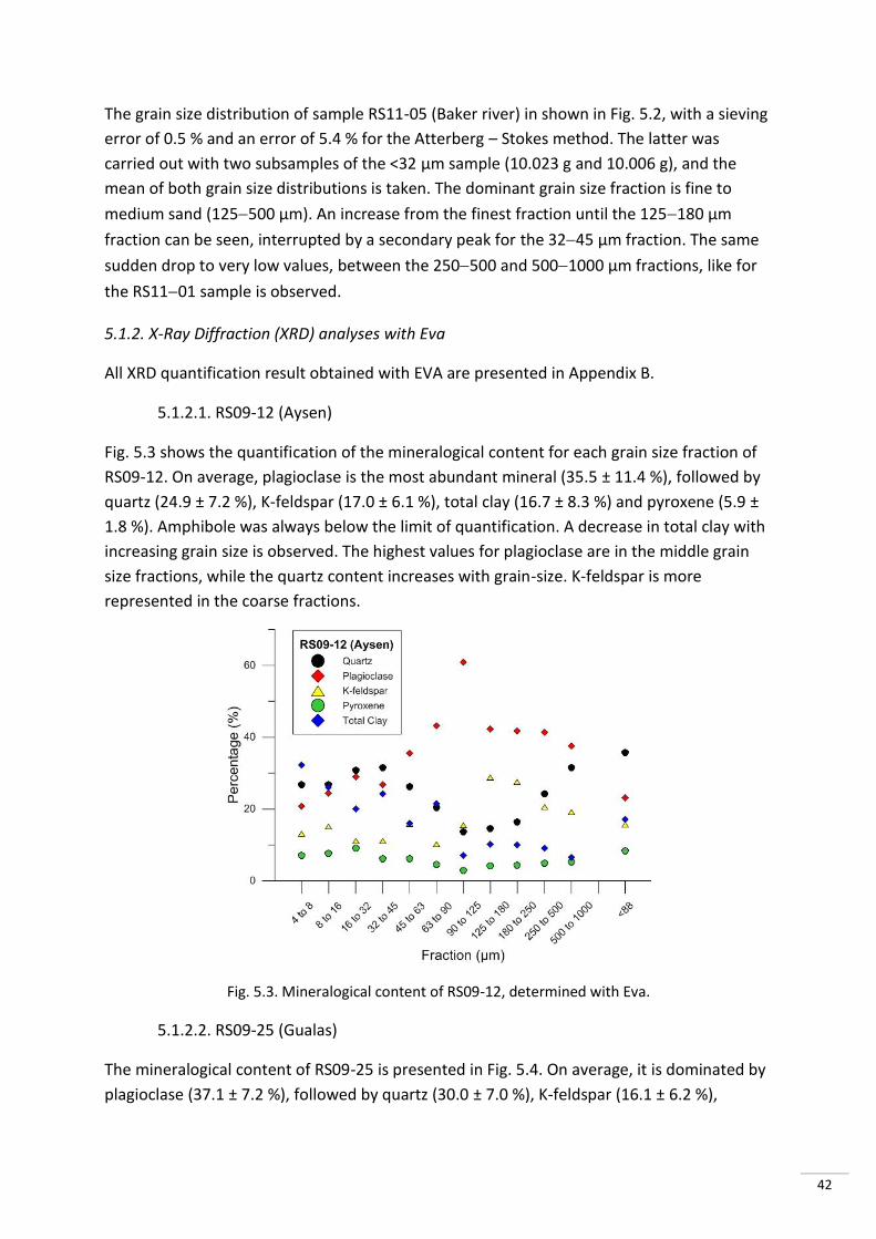
42
The grain size distribution of sample RS11-05 (Baker river) in shown in Fig. 5.2, with a sieving
error of 0.5 % and an error of 5.4 % for the Atterberg – Stokes method. The latter was
carried out with two subsamples of the <32 µm sample (10.023 g and 10.006 g), and the
mean of both grain size distributions is taken. The dominant grain size fraction is fine to
medium sand (125500 µm). An increase from the finest fraction until the 125180 µm
fraction can be seen, interrupted by a secondary peak for the 3245 µm fraction. The same
sudden drop to very low values, between the 250500 and 5001000 µm fractions, like for
the RS1101 sample is observed.
5.1.2. X-Ray Diffraction (XRD) analyses with Eva
All XRD quantification result obtained with EVA are presented in Appendix B.
5.1.2.1. RS09-12 (Aysen)
Fig. 5.3 shows the quantification of the mineralogical content for each grain size fraction of
RS09-12. On average, plagioclase is the most abundant mineral (35.5 ± 11.4 %), followed by
quartz (24.9 ± 7.2 %), K-feldspar (17.0 ± 6.1 %), total clay (16.7 ± 8.3 %) and pyroxene (5.9 ±
1.8 %). Amphibole was always below the limit of quantification. A decrease in total clay with
increasing grain size is observed. The highest values for plagioclase are in the middle grain
size fractions, while the quartz content increases with grain-size. K-feldspar is more
represented in the coarse fractions.
Fig. 5.3. Mineralogical content of RS09-12, determined with Eva.
5.1.2.2. RS09-25 (Gualas)
The mineralogical content of RS09-25 is presented in Fig. 5.4. On average, it is dominated by
plagioclase (37.1 ± 7.2 %), followed by quartz (30.0 ± 7.0 %), K-feldspar (16.1 ± 6.2 %),
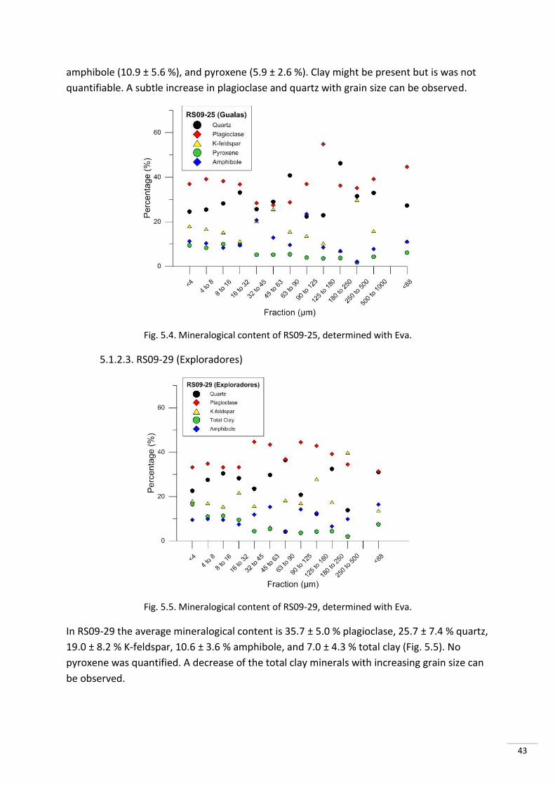
43
amphibole (10.9 ± 5.6 %), and pyroxene (5.9 ± 2.6 %). Clay might be present but is was not
quantifiable. A subtle increase in plagioclase and quartz with grain size can be observed.
Fig. 5.4. Mineralogical content of RS09-25, determined with Eva.
5.1.2.3. RS09-29 (Exploradores)
Fig. 5.5. Mineralogical content of RS09-29, determined with Eva.
In RS09-29 the average mineralogical content is 35.7 ± 5.0 % plagioclase, 25.7 ± 7.4 % quartz,
19.0 ± 8.2 % K-feldspar, 10.6 ± 3.6 % amphibole, and 7.0 ± 4.3 % total clay (Fig. 5.5). No
pyroxene was quantified. A decrease of the total clay minerals with increasing grain size can
be observed.

44
5.1.2.4. RS09-31 (Pelu)
The smallest grain size fraction of RS09-31 available (with enough sediment for XRD analysis)
is the <16 µm fraction. Plagioclase is clearly dominating the mineralogical assemblages, with
an average of 60.2 ± 10.8 %, followed by K-feldspar (12.5 ± 5.2 %), pyroxene (9.8 ± 4.9 %),
amphibole (9.5 ± 5.1 %), and quartz (8.0 ± 4.2 %). As can be seen in Fig. 5.6, plagioclase
generally increases with grain size. No clay is present.
Fig. 5.6 Mineralogical content of RS09-31, determined with Eva.
5.1.2.5. RS09-36 (Marinneli)
Fig. 5.7. Mineralogical content of RS09-36, determined with Eva.
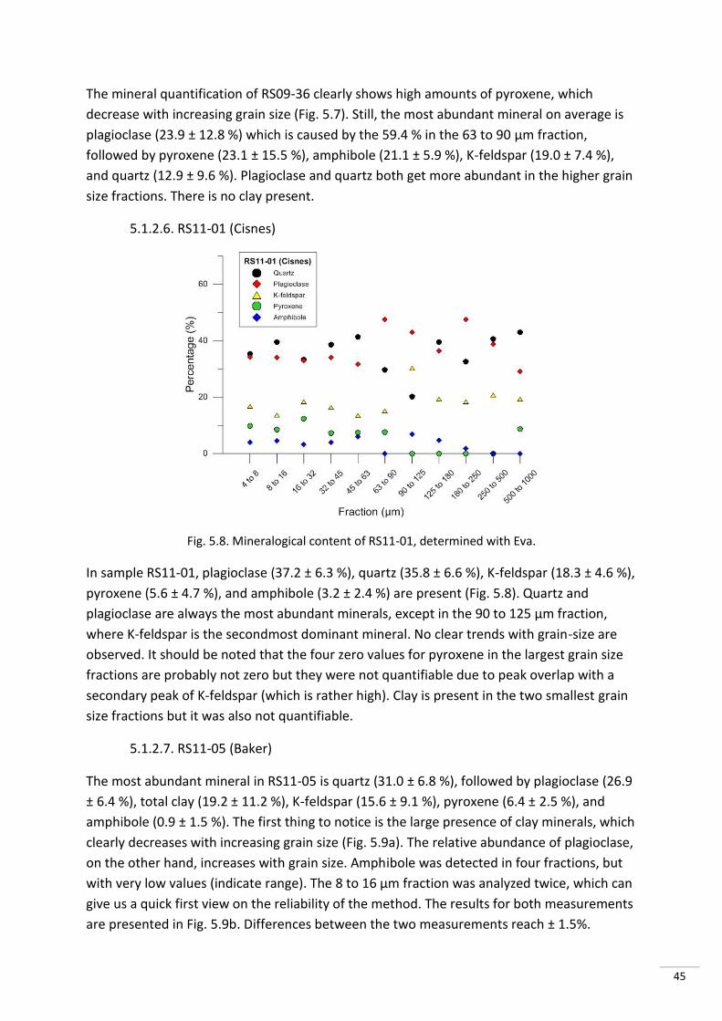
45
The mineral quantification of RS09-36 clearly shows high amounts of pyroxene, which
decrease with increasing grain size (Fig. 5.7). Still, the most abundant mineral on average is
plagioclase (23.9 ± 12.8 %) which is caused by the 59.4 % in the 63 to 90 µm fraction,
followed by pyroxene (23.1 ± 15.5 %), amphibole (21.1 ± 5.9 %), K-feldspar (19.0 ± 7.4 %),
and quartz (12.9 ± 9.6 %). Plagioclase and quartz both get more abundant in the higher grain
size fractions. There is no clay present.
5.1.2.6. RS11-01 (Cisnes)
Fig. 5.8. Mineralogical content of RS11-01, determined with Eva.
In sample RS11-01, plagioclase (37.2 ± 6.3 %), quartz (35.8 ± 6.6 %), K-feldspar (18.3 ± 4.6 %),
pyroxene (5.6 ± 4.7 %), and amphibole (3.2 ± 2.4 %) are present (Fig. 5.8). Quartz and
plagioclase are always the most abundant minerals, except in the 90 to 125 µm fraction,
where K-feldspar is the secondmost dominant mineral. No clear trends with grain-size are
observed. It should be noted that the four zero values for pyroxene in the largest grain size
fractions are probably not zero but they were not quantifiable due to peak overlap with a
secondary peak of K-feldspar (which is rather high). Clay is present in the two smallest grain
size fractions but it was also not quantifiable.
5.1.2.7. RS11-05 (Baker)
The most abundant mineral in RS11-05 is quartz (31.0 ± 6.8 %), followed by plagioclase (26.9
± 6.4 %), total clay (19.2 ± 11.2 %), K-feldspar (15.6 ± 9.1 %), pyroxene (6.4 ± 2.5 %), and
amphibole (0.9 ± 1.5 %). The first thing to notice is the large presence of clay minerals, which
clearly decreases with increasing grain size (Fig. 5.9a). The relative abundance of plagioclase,
on the other hand, increases with grain size. Amphibole was detected in four fractions, but
with very low values (indicate range). The 8 to 16 µm fraction was analyzed twice, which can
give us a quick first view on the reliability of the method. The results for both measurements
are presented in Fig. 5.9b. Differences between the two measurements reach ± 1.5%.
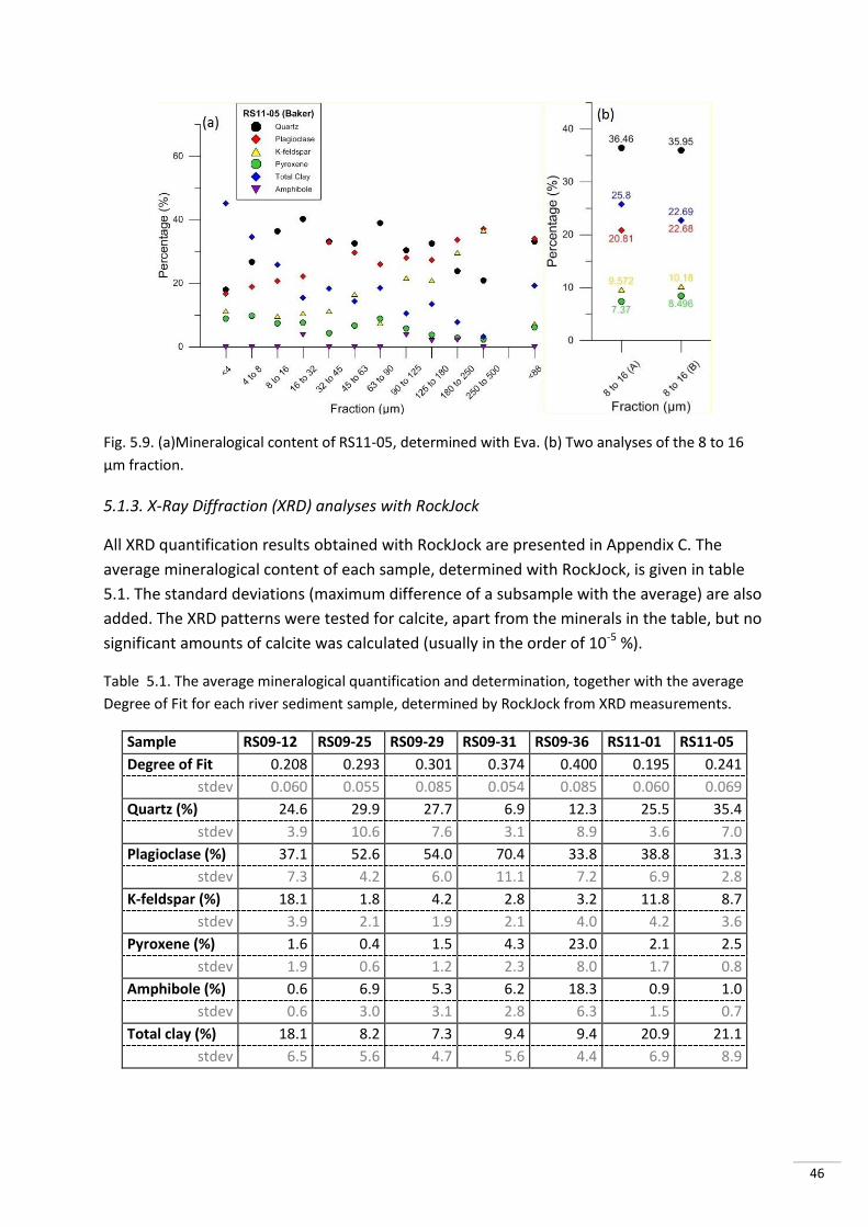
46
Fig. 5.9. (a)Mineralogical content of RS11-05, determined with Eva. (b) Two analyses of the 8 to 16
µm fraction.
5.1.3. X-Ray Diffraction (XRD) analyses with RockJock
All XRD quantification results obtained with RockJock are presented in Appendix C. The
average mineralogical content of each sample, determined with RockJock, is given in table
5.1. The standard deviations (maximum difference of a subsample with the average) are also
added. The XRD patterns were tested for calcite, apart from the minerals in the table, but no
significant amounts of calcite was calculated (usually in the order of 10-5 %).
Table 5.1. The average mineralogical quantification and determination, together with the average
Degree of Fit for each river sediment sample, determined by RockJock from XRD measurements.
Sample RS09-12 RS09-25 RS09-29 RS09-31 RS09-36 RS11-01 RS11-05
Degree of Fit 0.208 0.293 0.301 0.374 0.400 0.195 0.241
stdev 0.060 0.055 0.085 0.054 0.085 0.060 0.069
Quartz (%) 24.6 29.9 27.7 6.9 12.3 25.5 35.4
stdev 3.9 10.6 7.6 3.1 8.9 3.6 7.0
Plagioclase (%) 37.1 52.6 54.0 70.4 33.8 38.8 31.3
stdev 7.3 4.2 6.0 11.1 7.2 6.9 2.8
K-feldspar (%) 18.1 1.8 4.2 2.8 3.2 11.8 8.7
stdev 3.9 2.1 1.9 2.1 4.0 4.2 3.6
Pyroxene (%) 1.6 0.4 1.5 4.3 23.0 2.1 2.5
stdev 1.9 0.6 1.2 2.3 8.0 1.7 0.8
Amphibole (%) 0.6 6.9 5.3 6.2 18.3 0.9 1.0
stdev 0.6 3.0 3.1 2.8 6.3 1.5 0.7
Total clay (%) 18.1 8.2 7.3 9.4 9.4 20.9 21.1
stdev 6.5 5.6 4.7 5.6 4.4 6.9 8.9

47
5.1.3.1. RS09-12 (Aysen)
The relative mineralogical variations with grain size are presented in Fig. 5.10. Plagioclase is
the most abundant mineral with the highest abundance in the medium coarse grain size
fractions (45500 µm). A decreasing trend for the total clay content with increasing grain
size is also observed. The K-feldspar and quartz contents are lowest in the middle fractions.
Fig. 5.10. Mineralogical content of RS09-12, determined with RockJock.
5.1.3.2. RS09-25 (Gualas)
Fig. 5.11. Mineralogical content of RS09-25, determined with RockJock.
A dominance of plagioclase is observed in virtually each grain size fraction of river sediment
sample RS09-25 (Fig. 5.11). An increasing trend for quartz and decreasing trends for
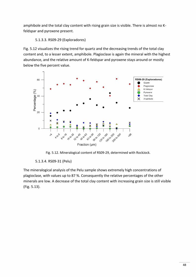
48
amphibole and the total clay content with rising grain size is visible. There is almost no K-
feldspar and pyroxene present.
5.1.3.3. RS09-29 (Exploradores)
Fig. 5.12 visualizes the rising trend for quartz and the decreasing trends of the total clay
content and, to a lesser extent, amphibole. Plagioclase is again the mineral with the highest
abundance, and the relative amount of K-feldspar and pyroxene stays around or mostly
below the five percent value.
Fig. 5.12. Mineralogical content of RS09-29, determined with RockJock.
5.1.3.4. RS09-31 (Pelu)
The mineralogical analysis of the Pelu sample shows extremely high concentrations of
plagioclase, with values up to 87 %. Consequently the relative percentages of the other
minerals are low. A decrease of the total clay content with increasing grain size is still visible
(Fig. 5.13).
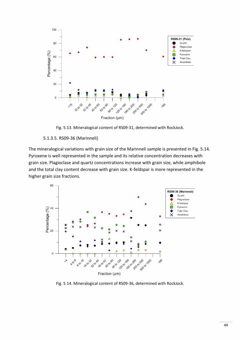
49
Fig. 5.13. Mineralogical content of RS09-31, determined with RockJock.
5.1.3.5. RS09-36 (Marinneli)
The mineralogical variations with grain size of the Marinneli sample is presented in Fig. 5.14.
Pyroxene is well represented in the sample and its relative concentration decreases with
grain size. Plagioclase and quartz concentrations increase with grain size, while amphibole
and the total clay content decrease with grain size. K-feldspar is more represented in the
higher grain size fractions.
Fig. 5.14. Mineralogical content of RS09-36, determined with RockJock.
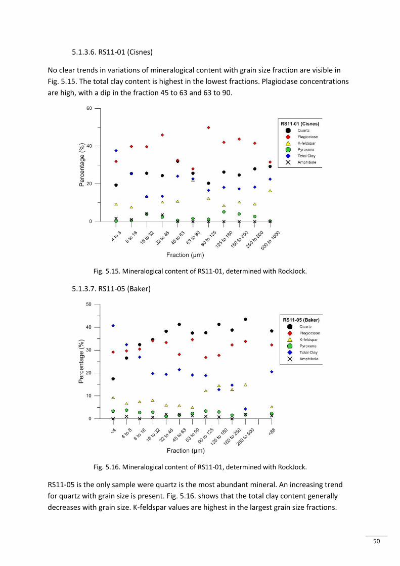
50
5.1.3.6. RS11-01 (Cisnes)
No clear trends in variations of mineralogical content with grain size fraction are visible in
Fig. 5.15. The total clay content is highest in the lowest fractions. Plagioclase concentrations
are high, with a dip in the fraction 45 to 63 and 63 to 90.
Fig. 5.15. Mineralogical content of RS11-01, determined with RockJock.
5.1.3.7. RS11-05 (Baker)
Fig. 5.16. Mineralogical content of RS11-01, determined with RockJock.
RS11-05 is the only sample were quartz is the most abundant mineral. An increasing trend
for quartz with grain size is present. Fig. 5.16. shows that the total clay content generally
decreases with grain size. K-feldspar values are highest in the largest grain size fractions.
51
Pyroxene and especially amphibole contents are very low. Plagioclase concentrations
fluctuate around 30 percent.
5.2. Simplified Geological Maps
The simplified geological maps of the northern and the southern study areas are shown in
Fig. 5.17 and Fig. 5.18 respectively. The lithological units are described in the legends of the
figures. Seven lithological units were created for the northern study area, and six for the
southern area. The alignment of the units is roughly North – South in the northern area, and
East – West in the southern area (except for the intrusive granitoids). The lithology
underneath the North Patagonian Icefield (NPI) is never directly determined but the NPI is
most likely underlain by the North Patagonian Batholith. The same is true for the Cordillera
Darwin Icefield (CDI). Here, a combination of intrusive and metamorphic (with both a
sedimentary and an intrusive protolite) rocks most likely underlie the CDI.
The watersheds in the northern study area, contoured by red lines on Fig. 5.17, are
numbered and named in the caption. The Baker and Aysen watersheds partly spread into
Argentina. The watershed of the Marinneli river (southern study area) was not mapped
because it lies almost completely under the ice field.
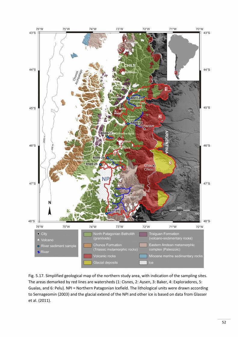
52
Fig. 5.17. Simplified geological map of the northern study area, with indication of the sampling sites.
The areas demarked by red lines are watersheds (1: Cisnes, 2: Aysen, 3: Baker, 4: Exploradores, 5:
Gualas, and 6: Pelu). NPI = Northern Patagonian Icefield. The lithological units were drawn according
to Sernageomin (2003) and the glacial extend of the NPI and other ice is based on data from Glasser
et al. (2011).
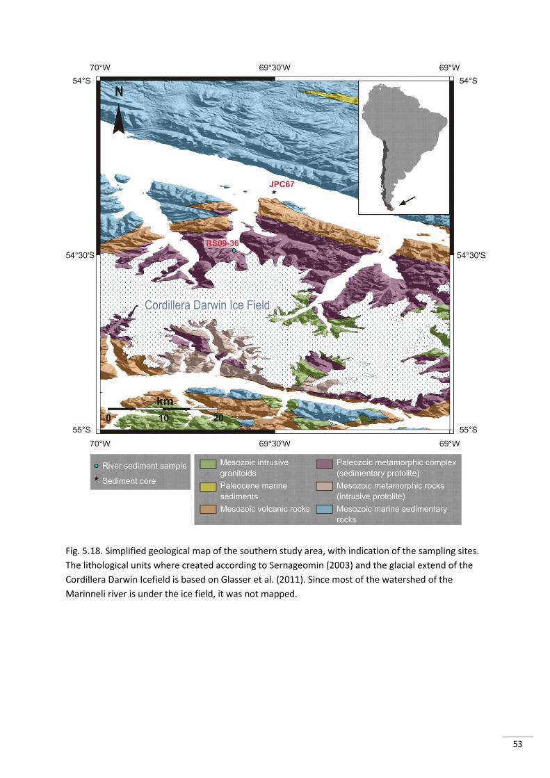
53
Fig. 5.18. Simplified geological map of the southern study area, with indication of the sampling sites.
The lithological units where created according to Sernageomin (2003) and the glacial extend of the
Cordillera Darwin Icefield is based on Glasser et al. (2011). Since most of the watershed of the
Marinneli river is under the ice field, it was not mapped.
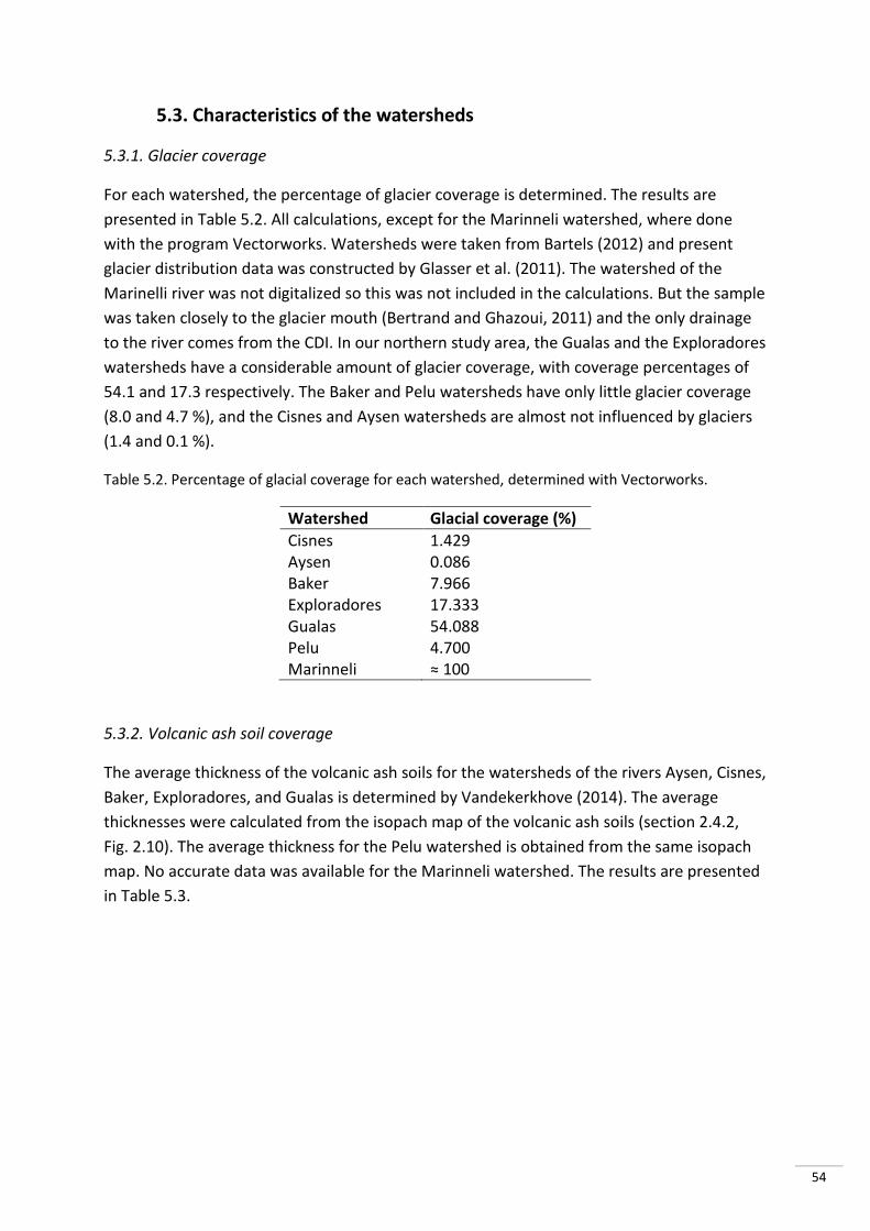
54
5.3. Characteristics of the watersheds
5.3.1. Glacier coverage
For each watershed, the percentage of glacier coverage is determined. The results are
presented in Table 5.2. All calculations, except for the Marinneli watershed, where done
with the program Vectorworks. Watersheds were taken from Bartels (2012) and present
glacier distribution data was constructed by Glasser et al. (2011). The watershed of the
Marinelli river was not digitalized so this was not included in the calculations. But the sample
was taken closely to the glacier mouth (Bertrand and Ghazoui, 2011) and the only drainage
to the river comes from the CDI. In our northern study area, the Gualas and the Exploradores
watersheds have a considerable amount of glacier coverage, with coverage percentages of
54.1 and 17.3 respectively. The Baker and Pelu watersheds have only little glacier coverage
(8.0 and 4.7 %), and the Cisnes and Aysen watersheds are almost not influenced by glaciers
(1.4 and 0.1 %).
Table 5.2. Percentage of glacial coverage for each watershed, determined with Vectorworks.
Watershed Glacial coverage (%)
Cisnes 1.429 Aysen 0.086 Baker 7.966 Exploradores 17.333 Gualas 54.088 Pelu 4.700 Marinneli ≈ 100
5.3.2. Volcanic ash soil coverage
The average thickness of the volcanic ash soils for the watersheds of the rivers Aysen, Cisnes,
Baker, Exploradores, and Gualas is determined by Vandekerkhove (2014). The average
thicknesses were calculated from the isopach map of the volcanic ash soils (section 2.4.2,
Fig. 2.10). The average thickness for the Pelu watershed is obtained from the same isopach
map. No accurate data was available for the Marinneli watershed. The results are presented
in Table 5.3.
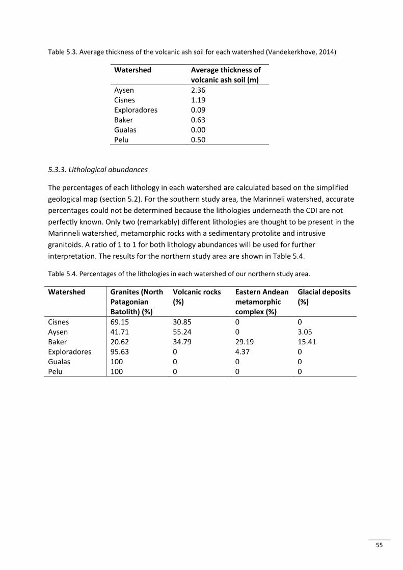
55
Table 5.3. Average thickness of the volcanic ash soil for each watershed (Vandekerkhove, 2014)
Watershed Average thickness of volcanic ash soil (m)
Aysen 2.36 Cisnes 1.19 Exploradores 0.09 Baker 0.63 Gualas 0.00 Pelu 0.50
5.3.3. Lithological abundances
The percentages of each lithology in each watershed are calculated based on the simplified
geological map (section 5.2). For the southern study area, the Marinneli watershed, accurate
percentages could not be determined because the lithologies underneath the CDI are not
perfectly known. Only two (remarkably) different lithologies are thought to be present in the
Marinneli watershed, metamorphic rocks with a sedimentary protolite and intrusive
granitoids. A ratio of 1 to 1 for both lithology abundances will be used for further
interpretation. The results for the northern study area are shown in Table 5.4.
Table 5.4. Percentages of the lithologies in each watershed of our northern study area.
Watershed Granites (North Patagonian Batolith) (%)
Volcanic rocks (%)
Eastern Andean metamorphic complex (%)
Glacial deposits (%)
Cisnes 69.15 30.85 0 0 Aysen 41.71 55.24 0 3.05 Baker 20.62 34.79 29.19 15.41 Exploradores 95.63 0 4.37 0 Gualas 100 0 0 0 Pelu 100 0 0 0
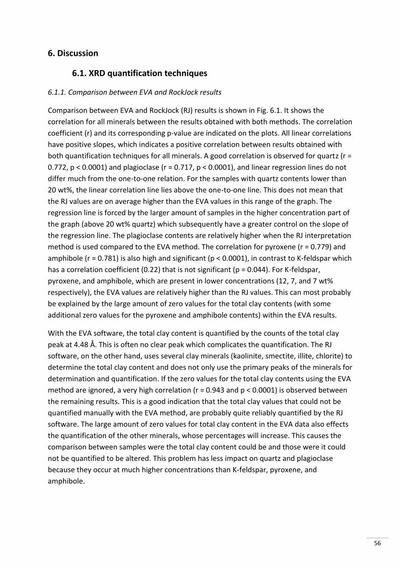
56
6. Discussion
6.1. XRD quantification techniques
6.1.1. Comparison between EVA and RockJock results
Comparison between EVA and RockJock (RJ) results is shown in Fig. 6.1. It shows the
correlation for all minerals between the results obtained with both methods. The correlation
coefficient (r) and its corresponding p-value are indicated on the plots. All linear correlations
have positive slopes, which indicates a positive correlation between results obtained with
both quantification techniques for all minerals. A good correlation is observed for quartz (r =
0.772, p < 0.0001) and plagioclase (r = 0.717, p < 0.0001), and linear regression lines do not
differ much from the one-to-one relation. For the samples with quartz contents lower than
20 wt%, the linear correlation line lies above the one-to-one line. This does not mean that
the RJ values are on average higher than the EVA values in this range of the graph. The
regression line is forced by the larger amount of samples in the higher concentration part of
the graph (above 20 wt% quartz) which subsequently have a greater control on the slope of
the regression line. The plagioclase contents are relatively higher when the RJ interpretation
method is used compared to the EVA method. The correlation for pyroxene (r = 0.779) and
amphibole (r = 0.781) is also high and significant (p < 0.0001), in contrast to K-feldspar which
has a correlation coefficient (0.22) that is not significant (p = 0.044). For K-feldspar,
pyroxene, and amphibole, which are present in lower concentrations (12, 7, and 7 wt%
respectively), the EVA values are relatively higher than the RJ values. This can most probably
be explained by the large amount of zero values for the total clay contents (with some
additional zero values for the pyroxene and amphibole contents) within the EVA results.
With the EVA software, the total clay content is quantified by the counts of the total clay
peak at 4.48 Å. This is often no clear peak which complicates the quantification. The RJ
software, on the other hand, uses several clay minerals (kaolinite, smectite, illite, chlorite) to
determine the total clay content and does not only use the primary peaks of the minerals for
determination and quantification. If the zero values for the total clay contents using the EVA
method are ignored, a very high correlation (r = 0.943 and p < 0.0001) is observed between
the remaining results. This is a good indication that the total clay values that could not be
quantified manually with the EVA method, are probably quite reliably quantified by the RJ
software. The large amount of zero values for total clay content in the EVA data also effects
the quantification of the other minerals, whose percentages will increase. This causes the
comparison between samples were the total clay content could be and those were it could
not be quantified to be altered. This problem has less impact on quartz and plagioclase
because they occur at much higher concentrations than K-feldspar, pyroxene, and
amphibole.

57
Fig. 6.1. Plots showing the correlation between mineral contents obtained using the EVA and
RockJock software. Black lines show the linear regression line and dashed blue lines show the one-to-
one correlation. The correlation coefficients (r), the p-values, and the slopes of the linear regression
lines (s) are added.
To investigate the impact of the large amount of zero values for the total clay content in the
EVA data on the correlation of the other minerals, a clay-free analysis was carried out. The
percentages were recalculated with a sum of 100 % for the five main minerals, without the
clay values. The result is shown in Fig. 6.2. The correlation of quartz, K-feldspar, and
pyroxene is higher for the clay-free analysis, but the correlation of plagioclase and
amphibole slightly decreased (values are indicated on the plots). The slopes of the linear
regression lines increased for all minerals, approaching more the one-to-one correlation.
These results confirm our explanation that the lack of data for the total clay content within
the EVA results affects the quantification of the other minerals, causing the slopes of the
linear regression lines to decrease. But apart from this clay-peak problem, the correlation is
still not perfect, indicating that there is some variability in the quantification by both
methods. It is generally assumed that the XRD values are valid ± 5 %. For our data, the
average absolute difference between all the RJ results and the EVA results is 7.5 % and 8.1 %
when the total clay content is not included.
The poor correlation for the K-feldspar contents of both methods is visible by the large
scatter of the values (Fig. 6.1), the small correlation coefficient (0.22), and the insignificant p-
value (0.044). With the clay-free analysis, the slope of the linear correlation line of K-feldspar
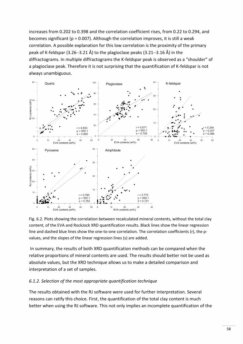
58
increases from 0.202 to 0.398 and the correlation coefficient rises, from 0.22 to 0.294, and
becomes significant (p = 0.007). Although the correlation improves, it is still a weak
correlation. A possible explanation for this low correlation is the proximity of the primary
peak of K-feldspar (3.263.21 Å) to the plagioclase peaks (3.213.16 Å) in the
diffractograms. In multiple diffractograms the K-feldspar peak is observed as a “shoulder” of
a plagioclase peak. Therefore it is not surprising that the quantification of K-feldspar is not
always unambiguous.
Fig. 6.2. Plots showing the correlation between recalculated mineral contents, without the total clay
content, of the EVA and RockJock XRD quantification results. Black lines show the linear regression
line and dashed blue lines show the one-to-one correlation. The correlation coefficients (r), the p-
values, and the slopes of the linear regression lines (s) are added.
In summary, the results of both XRD quantification methods can be compared when the
relative proportions of mineral contents are used. The results should better not be used as
absolute values, but the XRD technique allows us to make a detailed comparison and
interpretation of a set of samples.
6.1.2. Selection of the most appropriate quantification technique
The results obtained with the RJ software were used for further interpretation. Several
reasons can ratify this choice. First, the quantification of the total clay content is much
better when using the RJ software. This not only implies an incomplete quantification of the
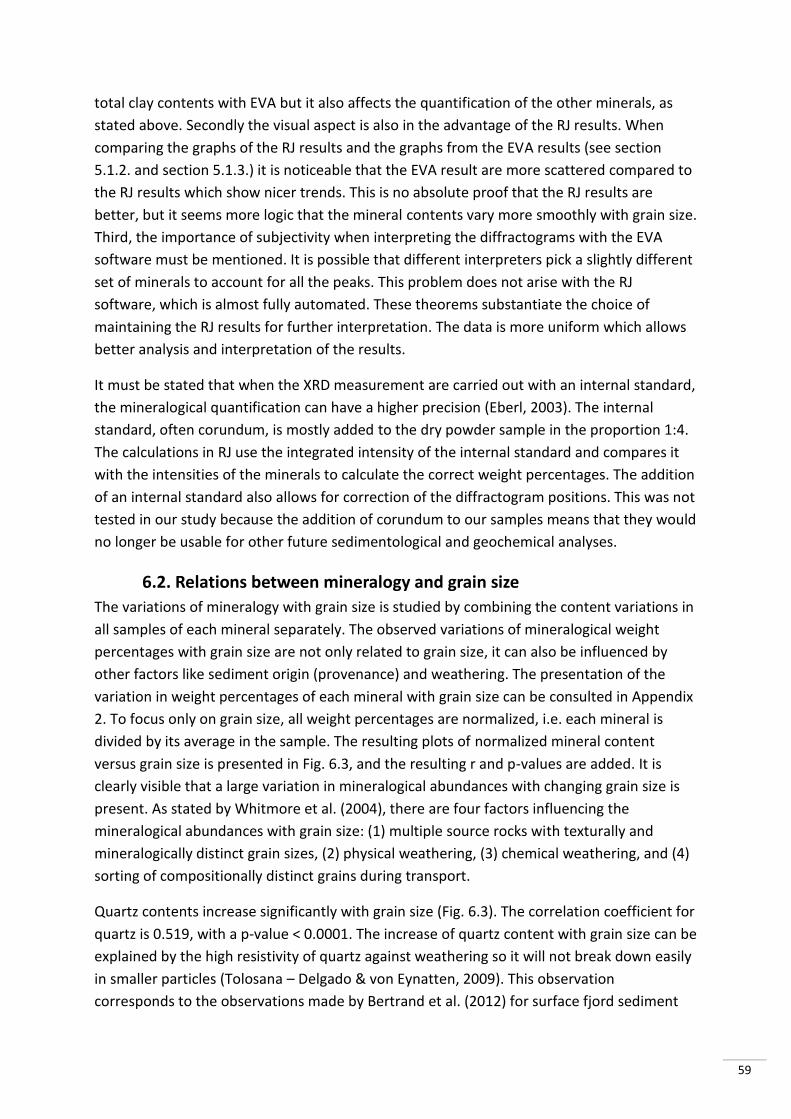
59
total clay contents with EVA but it also affects the quantification of the other minerals, as
stated above. Secondly the visual aspect is also in the advantage of the RJ results. When
comparing the graphs of the RJ results and the graphs from the EVA results (see section
5.1.2. and section 5.1.3.) it is noticeable that the EVA result are more scattered compared to
the RJ results which show nicer trends. This is no absolute proof that the RJ results are
better, but it seems more logic that the mineral contents vary more smoothly with grain size.
Third, the importance of subjectivity when interpreting the diffractograms with the EVA
software must be mentioned. It is possible that different interpreters pick a slightly different
set of minerals to account for all the peaks. This problem does not arise with the RJ
software, which is almost fully automated. These theorems substantiate the choice of
maintaining the RJ results for further interpretation. The data is more uniform which allows
better analysis and interpretation of the results.
It must be stated that when the XRD measurement are carried out with an internal standard,
the mineralogical quantification can have a higher precision (Eberl, 2003). The internal
standard, often corundum, is mostly added to the dry powder sample in the proportion 1:4.
The calculations in RJ use the integrated intensity of the internal standard and compares it
with the intensities of the minerals to calculate the correct weight percentages. The addition
of an internal standard also allows for correction of the diffractogram positions. This was not
tested in our study because the addition of corundum to our samples means that they would
no longer be usable for other future sedimentological and geochemical analyses.
6.2. Relations between mineralogy and grain size
The variations of mineralogy with grain size is studied by combining the content variations in
all samples of each mineral separately. The observed variations of mineralogical weight
percentages with grain size are not only related to grain size, it can also be influenced by
other factors like sediment origin (provenance) and weathering. The presentation of the
variation in weight percentages of each mineral with grain size can be consulted in Appendix
2. To focus only on grain size, all weight percentages are normalized, i.e. each mineral is
divided by its average in the sample. The resulting plots of normalized mineral content
versus grain size is presented in Fig. 6.3, and the resulting r and p-values are added. It is
clearly visible that a large variation in mineralogical abundances with changing grain size is
present. As stated by Whitmore et al. (2004), there are four factors influencing the
mineralogical abundances with grain size: (1) multiple source rocks with texturally and
mineralogically distinct grain sizes, (2) physical weathering, (3) chemical weathering, and (4)
sorting of compositionally distinct grains during transport.
Quartz contents increase significantly with grain size (Fig. 6.3). The correlation coefficient for
quartz is 0.519, with a p-value < 0.0001. The increase of quartz content with grain size can be
explained by the high resistivity of quartz against weathering so it will not break down easily
in smaller particles (Tolosana – Delgado & von Eynatten, 2009). This observation
corresponds to the observations made by Bertrand et al. (2012) for surface fjord sediment
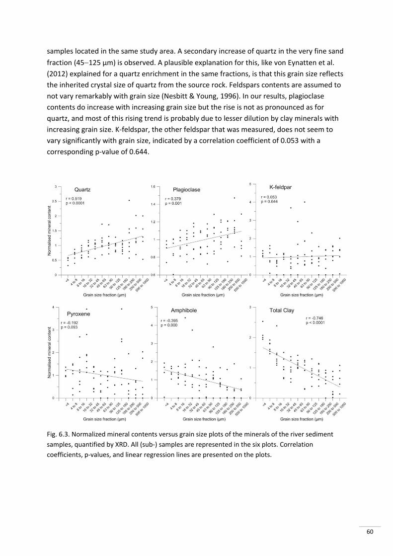
60
samples located in the same study area. A secondary increase of quartz in the very fine sand
fraction (45125 µm) is observed. A plausible explanation for this, like von Eynatten et al.
(2012) explained for a quartz enrichment in the same fractions, is that this grain size reflects
the inherited crystal size of quartz from the source rock. Feldspars contents are assumed to
not vary remarkably with grain size (Nesbitt & Young, 1996). In our results, plagioclase
contents do increase with increasing grain size but the rise is not as pronounced as for
quartz, and most of this rising trend is probably due to lesser dilution by clay minerals with
increasing grain size. K-feldspar, the other feldspar that was measured, does not seem to
vary significantly with grain size, indicated by a correlation coefficient of 0.053 with a
corresponding p-value of 0.644.
Fig. 6.3. Normalized mineral contents versus grain size plots of the minerals of the river sediment
samples, quantified by XRD. All (sub-) samples are represented in the six plots. Correlation
coefficients, p-values, and linear regression lines are presented on the plots.
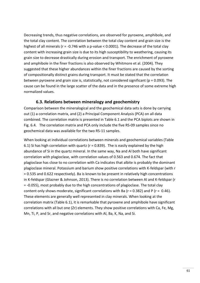
61
Decreasing trends, thus negative correlations, are observed for pyroxene, amphibole, and
the total clay content. The correlation between the total clay content and grain size is the
highest of all minerals (r = -0.746 with a p-value < 0.0001). The decrease of the total clay
content with increasing grain size is due to its high susceptibility to weathering, causing its
grain size to decrease drastically during erosion and transport. The enrichment of pyroxene
and amphibole in the finer fractions is also observed by Whitmore et al. (2004). They
suggested that these higher abundances within the finer fractions are caused by the sorting
of compositionally distinct grains during transport. It must be stated that the correlation
between pyroxene and grain size is, statistically, not considered significant (p = 0.093). The
cause can be found in the large scatter of the data and in the presence of some extreme high
normalized values.
6.3. Relations between mineralogy and geochemistry
Comparison between the mineralogical and the geochemical data sets is done by carrying
out (1) a correlation matrix, and (2) a Principal Component Analysis (PCA) on all data
combined. The correlation matrix is presented in Table 6.1 and the PCA biplots are shown in
Fig. 6.4. The correlation matrix and PCA only include the five RS-09 samples since no
geochemical data was available for the two RS-11 samples.
When looking at individual correlations between minerals and geochemical variables (Table
6.1) Si has high correlation with quartz (r = 0.839). The is easily explained by the high
abundance of Si in the quartz mineral. In the same way, Na and Al both have significant
correlation with plagioclase, with correlation values of 0.563 and 0.674. The fact that
plagioclase has close to no correlation with Ca indicates that albite is probably the dominant
plagioclase mineral. Potassium and barium show positive correlations with K-feldspar (with r
= 0.535 and 0.622 respectively). Ba is known to be present in relatively high concentrations
in K-feldspar (Glazner & Johnson, 2013). There is no correlation between Al and K-feldspar (r
= -0.055), most probably due to the high concentrations of plagioclase. The total clay
content only shows moderate, significant correlations with Ba (r = 0.382) and P (r = 0.46).
These elements are generally well represented in clay minerals. When looking at the
correlation matrix (Table 6.1), it is remarkable that pyroxene and amphibole have significant
correlations with all but one (Zr) elements. They show positive correlations with Ca, Fe, Mg,
Mn, Ti, P, and Sr, and negative correlations with Al, Ba, K, Na, and Si.

62
Table 6.1. Correlation matrix for the combined mineralogical – geochemical – grain size dataset.
Values in bold are different from zero with a significance level (p) smaller than 0.01. GS: grain size,
Qz: quartz, Plag: plagioclase, K-f: K-feldspar, Px: pyroxene, Amp: amphibole.
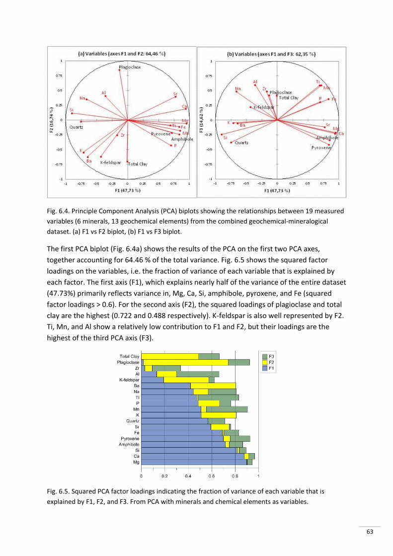
63
Fig. 6.4. Principle Component Analysis (PCA) biplots showing the relationships between 19 measured
variables (6 minerals, 13 geochemical elements) from the combined geochemical-mineralogical
dataset. (a) F1 vs F2 biplot, (b) F1 vs F3 biplot.
The first PCA biplot (Fig. 6.4a) shows the results of the PCA on the first two PCA axes,
together accounting for 64.46 % of the total variance. Fig. 6.5 shows the squared factor
loadings on the variables, i.e. the fraction of variance of each variable that is explained by
each factor. The first axis (F1), which explains nearly half of the variance of the entire dataset
(47.73%) primarily reflects variance in, Mg, Ca, Si, amphibole, pyroxene, and Fe (squared
factor loadings > 0.6). For the second axis (F2), the squared loadings of plagioclase and total
clay are the highest (0.722 and 0.488 respectively). K-feldspar is also well represented by F2.
Ti, Mn, and Al show a relatively low contribution to F1 and F2, but their loadings are the
highest of the third PCA axis (F3).
Fig. 6.5. Squared PCA factor loadings indicating the fraction of variance of each variable that is
explained by F1, F2, and F3. From PCA with minerals and chemical elements as variables.
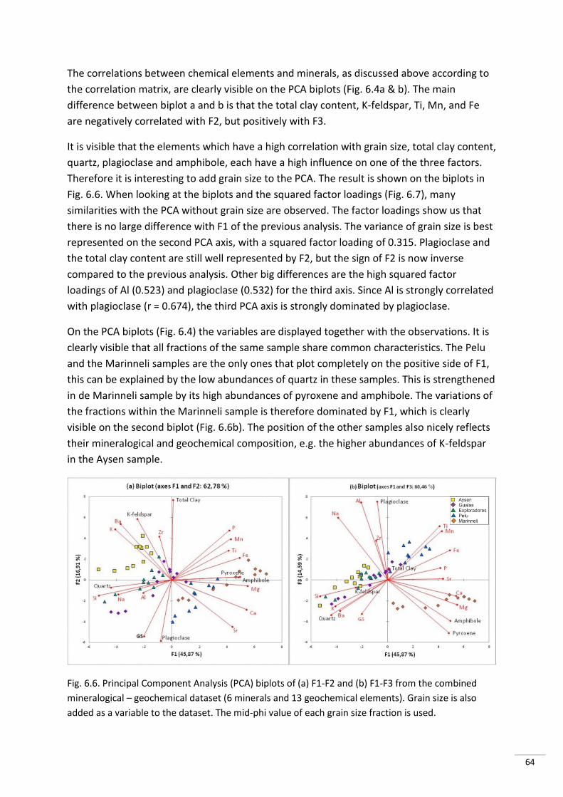
64
The correlations between chemical elements and minerals, as discussed above according to
the correlation matrix, are clearly visible on the PCA biplots (Fig. 6.4a & b). The main
difference between biplot a and b is that the total clay content, K-feldspar, Ti, Mn, and Fe
are negatively correlated with F2, but positively with F3.
It is visible that the elements which have a high correlation with grain size, total clay content,
quartz, plagioclase and amphibole, each have a high influence on one of the three factors.
Therefore it is interesting to add grain size to the PCA. The result is shown on the biplots in
Fig. 6.6. When looking at the biplots and the squared factor loadings (Fig. 6.7), many
similarities with the PCA without grain size are observed. The factor loadings show us that
there is no large difference with F1 of the previous analysis. The variance of grain size is best
represented on the second PCA axis, with a squared factor loading of 0.315. Plagioclase and
the total clay content are still well represented by F2, but the sign of F2 is now inverse
compared to the previous analysis. Other big differences are the high squared factor
loadings of Al (0.523) and plagioclase (0.532) for the third axis. Since Al is strongly correlated
with plagioclase (r = 0.674), the third PCA axis is strongly dominated by plagioclase.
On the PCA biplots (Fig. 6.4) the variables are displayed together with the observations. It is
clearly visible that all fractions of the same sample share common characteristics. The Pelu
and the Marinneli samples are the only ones that plot completely on the positive side of F1,
this can be explained by the low abundances of quartz in these samples. This is strengthened
in de Marinneli sample by its high abundances of pyroxene and amphibole. The variations of
the fractions within the Marinneli sample is therefore dominated by F1, which is clearly
visible on the second biplot (Fig. 6.6b). The position of the other samples also nicely reflects
their mineralogical and geochemical composition, e.g. the higher abundances of K-feldspar
in the Aysen sample.
Fig. 6.6. Principal Component Analysis (PCA) biplots of (a) F1-F2 and (b) F1-F3 from the combined
mineralogical – geochemical dataset (6 minerals and 13 geochemical elements). Grain size is also
added as a variable to the dataset. The mid-phi value of each grain size fraction is used.
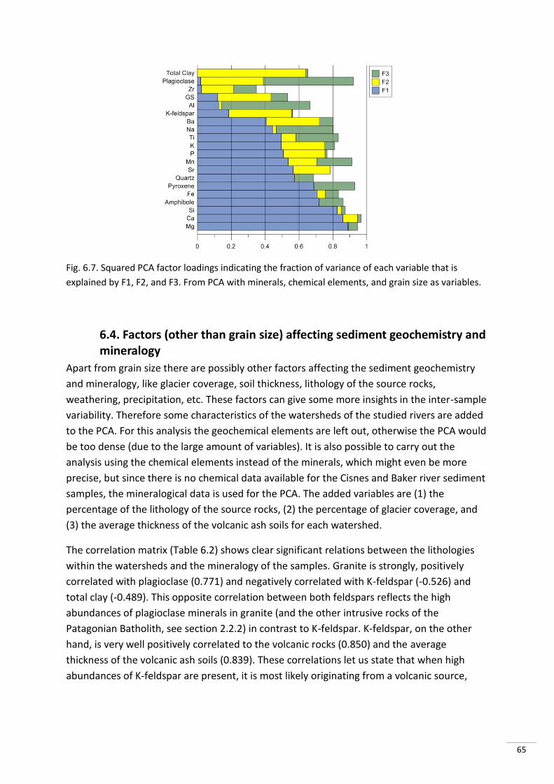
65
Fig. 6.7. Squared PCA factor loadings indicating the fraction of variance of each variable that is
explained by F1, F2, and F3. From PCA with minerals, chemical elements, and grain size as variables.
6.4. Factors (other than grain size) affecting sediment geochemistry and mineralogy
Apart from grain size there are possibly other factors affecting the sediment geochemistry
and mineralogy, like glacier coverage, soil thickness, lithology of the source rocks,
weathering, precipitation, etc. These factors can give some more insights in the inter-sample
variability. Therefore some characteristics of the watersheds of the studied rivers are added
to the PCA. For this analysis the geochemical elements are left out, otherwise the PCA would
be too dense (due to the large amount of variables). It is also possible to carry out the
analysis using the chemical elements instead of the minerals, which might even be more
precise, but since there is no chemical data available for the Cisnes and Baker river sediment
samples, the mineralogical data is used for the PCA. The added variables are (1) the
percentage of the lithology of the source rocks, (2) the percentage of glacier coverage, and
(3) the average thickness of the volcanic ash soils for each watershed.
The correlation matrix (Table 6.2) shows clear significant relations between the lithologies
within the watersheds and the mineralogy of the samples. Granite is strongly, positively
correlated with plagioclase (0.771) and negatively correlated with K-feldspar (-0.526) and
total clay (-0.489). This opposite correlation between both feldspars reflects the high
abundances of plagioclase minerals in granite (and the other intrusive rocks of the
Patagonian Batholith, see section 2.2.2) in contrast to K-feldspar. K-feldspar, on the other
hand, is very well positively correlated to the volcanic rocks (0.850) and the average
thickness of the volcanic ash soils (0.839). These correlations let us state that when high
abundances of K-feldspar are present, it is most likely originating from a volcanic source,
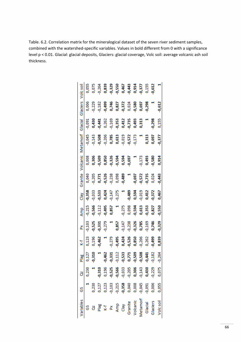
66
Table. 6.2. Correlation matrix for the mineralogical dataset of the seven river sediment samples,
combined with the watershed-specific variables. Values in bold different from 0 with a significance
level p < 0.01. Glacial: glacial deposits, Glaciers: glacial coverage, Volc soil: average volcanic ash soil
thickness.
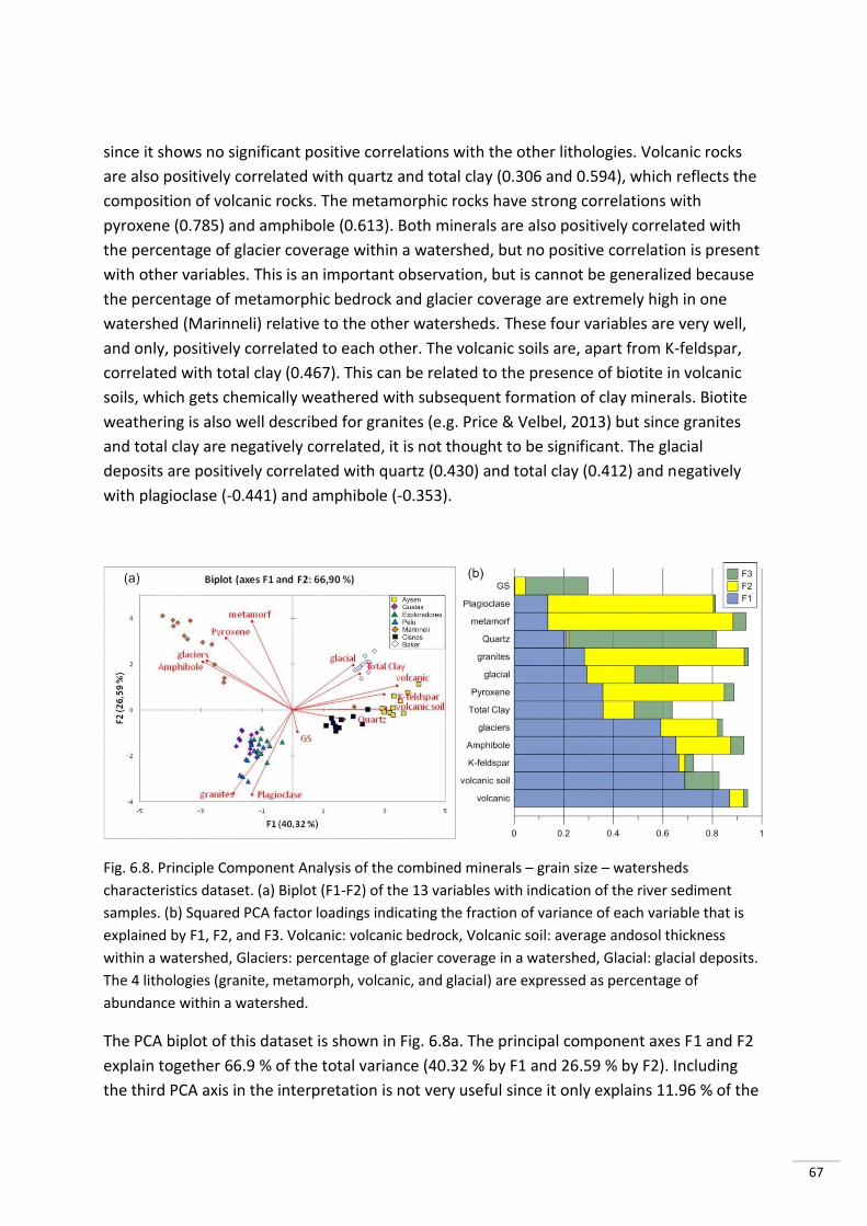
67
since it shows no significant positive correlations with the other lithologies. Volcanic rocks
are also positively correlated with quartz and total clay (0.306 and 0.594), which reflects the
composition of volcanic rocks. The metamorphic rocks have strong correlations with
pyroxene (0.785) and amphibole (0.613). Both minerals are also positively correlated with
the percentage of glacier coverage within a watershed, but no positive correlation is present
with other variables. This is an important observation, but is cannot be generalized because
the percentage of metamorphic bedrock and glacier coverage are extremely high in one
watershed (Marinneli) relative to the other watersheds. These four variables are very well,
and only, positively correlated to each other. The volcanic soils are, apart from K-feldspar,
correlated with total clay (0.467). This can be related to the presence of biotite in volcanic
soils, which gets chemically weathered with subsequent formation of clay minerals. Biotite
weathering is also well described for granites (e.g. Price & Velbel, 2013) but since granites
and total clay are negatively correlated, it is not thought to be significant. The glacial
deposits are positively correlated with quartz (0.430) and total clay (0.412) and negatively
with plagioclase (-0.441) and amphibole (-0.353).
Fig. 6.8. Principle Component Analysis of the combined minerals – grain size – watersheds
characteristics dataset. (a) Biplot (F1-F2) of the 13 variables with indication of the river sediment
samples. (b) Squared PCA factor loadings indicating the fraction of variance of each variable that is
explained by F1, F2, and F3. Volcanic: volcanic bedrock, Volcanic soil: average andosol thickness
within a watershed, Glaciers: percentage of glacier coverage in a watershed, Glacial: glacial deposits.
The 4 lithologies (granite, metamorph, volcanic, and glacial) are expressed as percentage of
abundance within a watershed.
The PCA biplot of this dataset is shown in Fig. 6.8a. The principal component axes F1 and F2
explain together 66.9 % of the total variance (40.32 % by F1 and 26.59 % by F2). Including
the third PCA axis in the interpretation is not very useful since it only explains 11.96 % of the
68
total variance. Only the factor loadings of F3 on quartz and grain size (which is actually more
represented by the forth PCA axis) are noteworthy. The squared loadings of the factors on in
each variable is represented in Fig. 6.8b. F1 is mostly dominated by the volcanic rocks, the
volcanic ash soil thickness and K-feldspar (0.870, 0.688, and 0.664 respectively), and F2 is
primarily controlled by the variance in metamorphic rocks, plagioclase, granite, and
pyroxene (0.748, 0.669, 0.645, and 0.491 respectively). Plagioclase and granite are
negatively correlated with the metamorphic rocks and pyroxene.
The PCA biplot (Fig. 6.8a) visualizes very well the correlations discussed above (based on the
correlation matrix), e.g. K-feldspar – volcanic ash soil – volcanic bedrock correlations,
plagioclase – granites correlation, glacier coverage – metamorphic bedrock – amphibole –
pyroxene correlations, etc. The river sediment samples are plotted and visualized on the
biplot. The fractions within each river sediment samples are even more closely spaced and
the river sediment samples seem more distinct from each other than in Fig. 6.6, the previous
PCA. The primary cause of this increased inter-sample variability is that the new variables are
constant within each watershed, each variable has the same value for all fractions of a
sample. Nevertheless these groupings can give us some variable information. Especially the
fact that almost all the minerals show very good correlation with one of these new variables
is important. This indicates that by knowing the mineralogy of a river sediment sample
within our study area, or an area with comparable characteristics, a well estimated guess can
be performed on the bedrock lithology, andosol coverage and influence by glaciers in the
watershed of the river.
6.5. Provenance and weathering
Carrying out a study of provenance and weathering can be done by looking at each sample
separately, but more information is often obtained by comparing the similarities and
differences between samples from different watersheds. The provenance determination
looks quite straight forward, since the correlations between mineralogy and bedrock
lithology is relatively good defined. However, weathering processes and other factors can
alter the mineralogy of the sample, masking the provenance signal, which in turn can give us
insights into these factors, like weathering, themselves. Therefore provenance and
weathering are discussed together. The mineral percentages mentioned below, are the
average abundances in each river sediment sample.
The river sediment sample RS09-12, collected from river Aysen, contains the second lowest
amount of plagioclase (37 %) but the highest amount of K-feldspar (18 %) on average,
compared to the other samples. This high percentage of K-feldspar is related to the large
abundance of volcanic bedrocks in the area (55.24 %) and/or the large average thickness of
volcanic ash soils (2.36 m). These volcanic rocks and, especially, the volcanic ash soils, are
more susceptible to weathering than granite, which forms the bedrock in 41.7 % of the area
of the watershed. Due to the fact that granite has a strong positive correlation with

69
plagioclase, and negative with K-feldspar and total clay (which is also relatively high in the
Aysen sample, 18 % on average), combined with the other observations, it probably does not
contribute much to the mineralogy and geochemistry of the river Aysen. The characteristics
of the Cisnes watershed, located North of the river Aysen, are very similar to those of the
Aysen watershed. The same bedrock lithologies are present (69.1 % granite, 30.9 % volcanic
rocks), both have almost no glaciers within their watershed (1.43 % glacier coverage for
Cisnes and 0.09 % for Aysen), and volcanic ash soils are also widespread (with an average
thickness of 1.19m). The average mineralogical abundances are also quite similar for both
samples. The lesser amount, but still high, of K-feldspar (11.8 %) most likely reflects the
thinner average volcanic ash soil and/or the relative smaller area where volcanic rocks form
the bedrock. It is a bit unfortunate that both volcanic soil thickness and abundance of
volcanic bedrock are smaller in the Cisnes watershed. If one of both would be higher than in
the Aysen watershed, it could possibly give us an idea whether the weathering product K-
feldspar finds its source predominantly in the volcanic ash soils or in the volcanic bedrock, or
in both. The high abundances of clay minerals (20.9 % in Cisnes and 18.1 % in Aysen) are
probably also caused by weathering of volcanic rocks and soils. The volcanic rocks yield
considerable amounts of biotite, which gets easily weathered. Clay minerals like kaolinite,
smectite and illite are also commonly present in volcanic ash soils. The weathering in these
precipitation controlled watershed is thus favored by the volcanic rocks and soils.
It is interesting to make a comparison, for provenance and weathering, between the Gualas
and the Pelu sample because both watersheds are characterized by the same bedrock (100
% granite). The big difference between both is the high influence of the NPI glaciers on the
Gualas watershed, which is for 54.08 % covered by glaciers, in contrast to the Pelu
watershed (4.7 % glacier coverage). A volcanic ash soil is present in the Pelu watershed, with
an average thickness of 0.5m, but not in the Gualas watershed. The fact that the Pelu sample
has a small average abundance of K-feldspar (2.8 %) indicates that the sample is barely
influenced by weathering of the volcanic soil. Thus, this setting is ideal to look at the
weathering of granite in both a glacial and a non glacial environment. The big mineralogical
differences between both samples are observed for quartz (29.9 % in Gualas, 6.9 % in Pelu)
and plagioclase (52.6 % in Gualas, 70.4 % in Pelu). This indicates that the weathering of
granites in precipitation controlled areas (Pelu) is dominated by the selective weathering of
plagioclase, whereas in areas with a large glacial influence (Gualas) the granite weathering
also breaks down quartz minerals. The weathering of quartz from granite in cold
environments is also observed by French & Guglielmin (2001), with the difference that they
described it for extremely cold and dry environments (Antarctica) while Patagonia is known
for its high precipitation. The mineralogical abundances of the Exploradores river sediment
sample (27.7 % quartz and 54.0 % plagioclase) are very similar to those of the Gualas sample.
The Exploradores watershed is also influenced by glaciers from the NPI (17.33 % glacier
coverage) and its dominant bedrock lithology is also granite (95.63 %). The watershed has an
average volcanic ash soil thickness of 9 cm, which is probably reflected in the average 4.2 %
K-feldspar of the Exploradores sample. This 4.2 % of K-feldspar could also be the product of
70
granite (which can also yield small proportions of K-feldspar) weathering but since almost no
K-feldspar is present in the Gualas and Pelu samples, it is more likely to be the weathering
product of volcanic ash soils.
The Marinneli sample, collected at the northern side of the CDI, is the only sample for which
the watershed of the river is nearly 100 % covered by glaciers. Two bedrock lithologies are
present, granite and metamorphic rocks with a sedimentary protolite. Both lithologies are
estimated to cover 50 % of the watershed. The Marinneli sample contains very high
percentages of amphibole and pyroxene (18.3 % and 23.0 % respectively). 9.4 % total clay,
3.2 % K-feldspar, 33.8 % plagioclase, and 12.3 % quartz complete the average mineralogical
composition of the sample. The Marinneli sample is the most distinct from all to other
samples (Fig. 6.8a). The reason for this can be found in the extreme high abundances of
amphibole and pyroxene, compared to the other samples. The high abundance of amphibole
indicate that the metamorphic rock is the source rock of our sediment. Another argument to
state this assumption is the fact that pyroxene has a high susceptibility to weathering. This
means that if there is pyroxene present in the granites, it would also be present in higher
abundances in other samples. On the other hand, this watershed is located far away from
the other watersheds so differences in the composition of the granites are possible. Hervé
et al. (2008) determined the presence of fine grained meta-pelites to medium grained
schists nearby the Patagonian Batholith and satellite plutons. These metamorphic rocks
contain low-pressure amphibolite facies mineral assemblages, including amphibole, quartz,
biotite, muscovite, albite, and K-feldspar. Certain pyroxene minerals are often related to the
low-pressure amphibolite facies. Biotite and muscovite are known to weather easily to clay
minerals (e.g. kaolinite). It is plausible that this metamorphic composition is the source rock
for the sediment of the Marinneli sample. This could be an indication that chemical
weathering takes place in glacial environments.
The sample collected at the river Baker has the highest average abundances for quartz (35.4
%) and total clay (21.1 %), and the lowest for plagioclase (31.3 %). The watershed of the this
river is also interesting because it contains all four bedrock types (20.6 % granite, 34.8 %
volcanic rocks, 29.2 % metamorphic rocks, 15.4 % glacial deposits), it is influenced by the NPI
(but not totally), and it has an average volcanic ash soil thickness of 0.63 m. When looking at
the biplot in Fig. 6.8a, it can be seen that the subsamples of the Baker sample do not have
very high correlation with a specific bedrock lithology (except for glacial deposits but this
bedrock type is almost only present in the Baker watershed). This is quite logic since all
bedrock types are present in this watershed, which makes it also more difficult to determine
the provenance of the sediment. The K-feldspar present (8.7 %) is most likely the weathering
product of volcanic material. Since the plagioclase content is the lowest of all samples,
contribution of granitic weathering product to the sample does not seem likely. This is in
contrast with the strong seasonality of the water discharge rate of the river, which is mostly
controlled by glacier melt. A possible explanation is that granite does contribute to the
sediments in the river, in combination with the other lithologies. This explanation is
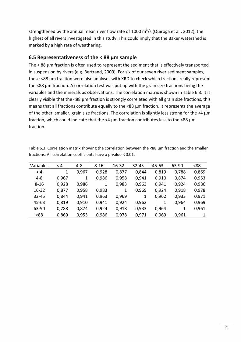
71
strengthened by the annual mean river flow rate of 1000 m3/s (Quiroga et al., 2012), the
highest of all rivers investigated in this study. This could imply that the Baker watershed is
marked by a high rate of weathering.
6.5 Representativeness of the < 88 µm sample
The < 88 µm fraction is often used to represent the sediment that is effectively transported
in suspension by rivers (e.g. Bertrand, 2009). For six of our seven river sediment samples,
these <88 µm fraction were also analyses with XRD to check which fractions really represent
the <88 µm fraction. A correlation test was put up with the grain size fractions being the
variables and the minerals as observations. The correlation matrix is shown in Table 6.3. It is
clearly visible that the <88 µm fraction is strongly correlated with all grain size fractions, this
means that all fractions contribute equally to the <88 µm fraction. It represents the average
of the other, smaller, grain size fractions. The correlation is slightly less strong for the <4 µm
fraction, which could indicate that the <4 µm fraction contributes less to the <88 µm
fraction.
Table 6.3. Correlation matrix showing the correlation between the <88 µm fraction and the smaller
fractions. All correlation coefficients have a p-value < 0.01.
Variables < 4 4-8 8-16 16-32 32-45 45-63 63-90 <88
< 4 1 0,967 0,928 0,877 0,844 0,819 0,788 0,869 4-8 0,967 1 0,986 0,958 0,941 0,910 0,874 0,953
8-16 0,928 0,986 1 0,983 0,963 0,941 0,924 0,986 16-32 0,877 0,958 0,983 1 0,969 0,924 0,918 0,978 32-45 0,844 0,941 0,963 0,969 1 0,962 0,933 0,971 45-63 0,819 0,910 0,941 0,924 0,962 1 0,964 0,969 63-90 0,788 0,874 0,924 0,918 0,933 0,964 1 0,961
<88 0,869 0,953 0,986 0,978 0,971 0,969 0,961 1
72
7. Conclusions
Comparison between the EVA and RockJock results indicate that the mineralogical
identification and quantification is better when using the RockJock XRD quantification
technique. This is proven by the more complete quantification of the total clay content, the
nicer trends and less scatter between the results, and the absence of subjectivity when using
the RockJock method. This results in more complete, uniform mineralogical data.
The overall mineralogy of the river sediment samples is dominated by the presence of
plagioclase (45.42%), followed by quartz (23.19%), total clay (13.47%), K-feldspar (7.24%),
amphibole (5.61%) and pyroxene (5.05%). Variations in normalized mineral content with
grain size reflect the grain size dependency of minerals. Positive correlations are observed
for quartz (r= 0.519) and plagioclase (r= 0.379), and negative correlations for total clay (r= -
0.746) and amphibole (r= -0.395), with a significance level p < 0.01. Strong correlations are
present between the geochemical and mineralogical data. As expected, strong significant
(p<0.01) correlations are present between Si and quartz ( 839), Na and plagioclase (0.663),
and Al and plagioclase (0.674). No close correlation between Ca and plagioclase is present,
which indicates dominancy of albite in the plagioclase. K and Ba show good correlation with
K-feldspar (0.535 and 0.622 respectively). Pyroxene and amphibole both have significant
positive correlations with Ca, Fe, Mg, Mn, Ti, P, and Sr, and negative with Al, Ba, K, Na, Si.
The Principal Components Analysis from the combined mineralogical-geochemical dataset
clearly shows the inter-river sample variability. All subsamples of one river sediment sample
share common characteristics and differ from the other samples, indicating the influence of
other factors, other than grain size, affecting sediment mineralogy.
The bedrock lithology within a watershed has a high influence on the river sediment
mineralogy, as well as the average volcanic ash soil thickness, and the percentage of glacier
coverage within a watershed. Granite is strongly, positively correlated with plagioclase
(0.771) and negatively with K-feldspar (-0.526) and total clay (-0.489). K-feldspar shows a
high correlation with the volcanic bedrocks (0.850) and with the average thickness of the
volcanic ash soils (0.839). Thus, K- feldspar is a good provenance indicator, high abundances
of K-feldspar in river sediment samples reflect erosion of volcanic soils or bedrock, since it
has no positive correlations with other lithologies. Pyroxene and amphibole have strong
correlations with metamorphic bedrocks (0.785 and 0.613 respectively) and the percentage
of glacier coverage. This observation cannot be generalized because the percentage of
metamorphic bedrock and glacier coverage are extremely high in one watershed (Marinneli)
relative to the other watersheds. The positive correlation between the average volcanic soil
thickness en the total clay content (0.467) probably results from the chemical weathering of
biotite to clay minerals.
73
Weathering activity in the precipitation controlled watersheds, Aysen and Cisnes,
predominantly occurs in the volcanic bedrock and/or in the volcanic soils, indicated by the
high amounts of K-feldspar and total clay in their river sediment samples. An environmental
control on granite weathering is observed. The weathering of granites in precipitation
controlled areas (Pelu watershed) is dominated by the selective weathering of plagioclase,
whereas in areas with a large glacial influence (Gualas watershed) the granite weathering
also breaks down quartz minerals. In de Marinneli watershed, which is fully covered by
glaciers, the metamorphic rocks are most likely predominantly weathered above the
granites, which is indicated by the high amount of pyroxene and amphibole. Almost 10 % of
clay is present in the Marinneli river sediment sample. These clays could possibly be the
weathering products of biotite and muscovite, which are present in the metamorphic rocks,
and which are known to weather easily to clay minerals (e.g. kaolinite). This is an indication
that chemical weathering of biotite and muscovite into clay minerals takes place in glacial
environments. The Baker watershed is possible characterized by a high rate of weathering.
Reasons for this statement are found in the high seasonality of the water discharge rate of
the river, controlled by glacier melting. This would imply a large contribution of weathered
granite material, which underlies the glaciers, but this is not the case (its plagioclase content
is the lowest of all samples).
The <88 µm fraction corresponds to the average of the seven fractions in which it was
separated. Each of the fractions contributes almost equally to the <88 µm fraction, with the
exception of the <4 µm fraction. This lowest fraction shows a slightly less strong correlation
with the <88 µm fraction, which may indicate that it contributes less than the other
fractions.
It would be interesting to carry out further research on this topic. This study clearly shows
that a lot of information is present in river sediment samples. The conclusions of this study
could be strengthened if more rivers would be investigated. Personally, I think it would be
very interesting to carry out a similar research, but more focused on the proglacial rivers.
The effect of global warming on glacial environments will be very large, the weathering
processes will adapt to the new conditions. This subsequently will have a great effect on the
amount of material transported through rivers and also on the composition of the material.
74
8. References
Aravena, J., Luckman, B.H., 2009, Spatio-temporal rainfall patterns in southern South
America, International Journal of Climatology. 29, 21062120.
Bartels, A., 2012, Aard en verspreiding van vulkanische bodems in Noord-Patagonië, Chili,
MSc thesis, Ghent University, Belgium.
Bertrand, S., 2009, National Geographic CRE Project Report; Towards a better interpretation
of sedimentary paleoclimate proxies in the fjords of Chilean Patagonia: Geochemical
characterization of the sediment sources – January 10 – February 9, 2009, 111.
Bertrand, S., 2011, Expedition Report: Sedimentary geochemistry of North Patagonian rivers:
Understanding the terrestrial processes recorded in Chilean fjord sediments – October 29 –
November 23, 2011, 121.
Bertrand, S., Hughen, K.A., Sepúlveda, J., Pantoja, S., 2012, Geochemistry of surface
sediments from the fjords of Northern Chilean Patagonia (4447°S): Spatial variability and
implications for paleoclimate reconstructions, Geochimica et Cosmochimica Acta, 76,
125146.
Bertrand, S., Hughen, K., Sepúlveda, J., Pantoja, S., 2014, Covariability of precipitation
seasonality and sea surface temperature in northern Chilean Patagonia during the late
Holocene, Submitted for Quaternary Science Revieuws.
Blunier, T., Chappellaz, J., Schwander, J., Dallenbach, A., Stauffer, B., Stocker, T.F., Raynaud,
D., Jouzel, J., Clausen, H.B., Hammer, C.U., Johnsen, S.J., 1998, Asynchrony of Antarctic and
Greenland climate change during the last glacial period, Nature, 394, 739743.
Bluth, G.J.S., Kump, L.R., 1994, Lithologic and climatologic controls of river chemistry,
Geochimica et Cosmochimica Acta, 58(10), 23412359.
Boutonnet, E., Arnaud, N., Guivel, C., Lagabrielle, Y., Scalabrino, B., Espinoza, F., 2010,
Subduction of the South Chile active spreading ridge: A 17 Ma to 3 Ma magmatic record in
central Patagonia (western edge of Meseta del lago Buenos Aires, Argentina), Journal of
Volcanology and Geothermal Research, 189, 319339.
Brown, G., Brindley, G.W., 1980, X-ray diffraction procedures for clay mineral identification.
In Brindley, G.W., and Brown, G. (Eds.), Crystal Structures of Clay Minerals and Their X-ray
Identification. Mineral. Soc. Monogr. London, 5, 305359.
Calvete, C., Sobarzo, M., 2011, Quantification of the surface brackish water layer and frontal
zones in southern Chilean fjords between Boca del Guafo (43°30’S) and Estero Elefantes
(46°30’S), Continental Shelf Research, 31, 162171.
75
Clapperton, C.M., 1993, Nature of environmental changes in South America at the Last
Glacial Maximum, Palaeogeography, Palaeoclimatology, Palaeoecology, 101, 189208.
Corbella, H., Lara, L., 2008, Late Cenozoic Quaternary volcanism in Pategonia and Tierra del
Fuego, In: Rabasse, J., The late Cenozoic of Patagonia and Tierra del Fuego, Developments in
Quaternary Sciences, 11, 95119.
Cunningham, W. D., 1995, Orogenesis at the southern tip of the Americas: the structural
evolution of the Cordillera Darwin metamorphic complex, southernmost Chile,
Tectonophysics, 244, 197229.
Depetris, P.J., Pasquini, A.I., Lecomte, K.L., 2014, Weathering and the Riverine Denudation of
Continents, Dordrecht: Springer Netherlands.
Ellies, A., Horn, R., Smith, R., 2000, Effects of management of a volcanic ash soil on structural
properties, International Agrophysics, 14, 377384.
Ericson, J.E., Mackenzie, J.D., Berger, R., 1976, Physics and chemistry of hydration process in
obsidians I: theoretical implication. In Advances in obsidian glass studies. (Taylor, R.E.;
editor). Noyes Press, 2545.
Fontijn, K., Lachowycz, S.M., Rawson, H., Pyle, D.M., Mather, T.A., Naranjo, J.A., Moreno-
Roa, H., 2014, Late Quaternary tephrostratigraphy of southern Chile and Argentina,
Quaternary Science Reviuews, 89, 7084.
French, H.M., Guglielmin, M., 2001, Cryogenic Weathering of Granite, Northern Victoria
Land, Antarctica, Permafrost Periglac. Process., 11, 305314.
Gerreaud, R., Lopez, P., Minvielle, M., Rojas, M., 2013, Large-scale Control on the Patagonian
Climate, Journal of Climate, 26, 215-230.
Harris, N., 1995, Significance of weathering Himalayan metasedimentary rocks and
leucogranites for the Sr isotope evolution of seawater during the early Miocene, Geology,
23, 795798.
Ghazoui, Z., 2011, Sédimentation récente dans les fjords de Patagonie Chilienne:
Caractérisation des sources sédimentaires et implication pour la reconstruction des
changements environnementaux au cours de l’Holocène, MSc thesis, Université Libre de
Bruxelles, Belgium.
Glasser, N. F., Harrison, S., Jansson, K. N., Anderson, K. ,Cowley, A., 2011, Global sea-level
contribution from Patagonian Icefields since the Little Ice Age maximum, Nature Geoscience,
1122, 303–307.
76
Glasser, N.F., Harrison, S., Winchester, V., Aniya, M., 2004, Late Pleistocene and Holocene
palaeoclimate and glacier fluctuations in Patagonia, Global and Planetary Change, 43,
79101.
Glazner, A.F., Johnson, B.R., 2013, Late crystallization of K-feldspar and the paradox of
megacrystic granites, Contributions to Mineralogy and Petrology, 166(3), 777799.
Gut, B., 2008, Geology, climate, and soils of Patagonia. In Gut, B., Trees in Patagonia, pp
918.
Gutiérrez, F., Gioncada, A., González Ferran, O., Lahsen, A., Mazzuoli, R., 2005, The Hudson
Volcano and surrounding monogenetic centres (Chilean Patagonia): An example of volcanism
associated with ridge-trench collision environment, Journal of Volcanology and Geothermal
Research, 145, 207233.
Hall, K., Arocena, J. M., Boelhouwers, J., Liping, Z., 2005, The influence of aspect on the
biological weathering of granites: observations from the KUNLUN Mountains, China,
Geomorphology, 67, 171188.
Hall, K., Thorn, C.E., Matsuoka, N., Prick, A., 2002, Weathering in cold regions: some
thoughts and perspectives, Progress in Physical Geography, 26(4), 577603.
Hervé, F., Calderón, M., Faúndez, V., 2008, The metamorphic complexes of the Patagonian
and Feugian Andes, Geologica Acta, 6(1), 4353.
Hervé, F., Pankhurst, R.J., Fanning, C.M., Calderón, M., Yaxley, G.M., 2007, The South
Patagonian batholiths: 150 my of granite magmatism on a plate margin, Lithos, 97, 373394.
Humphreys, E., 2009, Relation of flat subduction to magmatism and deformation in the
western United States, Geological Society of America Memoirs, 204, 8598.
Jolliffe, I.T., 1989, Rotation of 3-defined Principal Components, Applied Statistics, 38(1),
139147.
Kelly, E.F., Chadwick, O.A., Hilinski, T.F., 1998, The effect of plants on mineral weathering,
Biochemistry, 42, 2153.
Kilian, R., Hohner, M., Biester, H., Wallrabe-Adams, H.J., Stern, C.R., 2003, Holocene peat and
lake sediment tephra recors from the Chilean Andes (5355°S), Revista Geológico de Chile,
30(1), p. 2337.
Lagabrielle, Y., Guivel, C., Maury, R.C., Bourgois, J., Fourcade, S., Martin, H., 2000, Magmatic-
tectonic effects of high thermal regime at the site of active ridge subduction: the Chile Triple
Junction model, Tectonophysics, 326, 255268.
77
Lagabrielle, Y., Scalabrino, B., Suárez, M., Ritz, J.F., 2010, Mio-Pliocene glaciations of Central
Patagonia: New evidence and tectonic implications, Andean Geology, 37(2), 276299.
Lallemand, S., Heuret, A., Boutelier, D., 2005, On the relationschip between slab dip, back-
arc stress, upper plate absolute motion, and crustal nature in subduction zones,
Geochemistry Geophysics Geosystems, 6(9), 31–51.
Lee, B., Yeongcheol, H., Youngsook, H., Lundstrom, C., Siame, L.L., Lee, J.I., Park, B.K., 2013,
Chemical and physical weathering in south Patagonian rivers: A combined Sr-U-Be isotope
approach. Geochimica et Cosmochimica Acta, 101, 173190.
Lopez, P., Chevalier, P., Favier, V., Pouyaud, B., Ordenes, F., Oelemans, J., 2010, A regional
view of fluctuations in glacier length in southern South America, Global and Planetary
Change, 71, 85108.
Loring, D.H., Rantala, R.T.T, 1992, Manual for the geochemical analyses of marine sediments
and suspended particulate matter, Earth-Science Reviews, 32(4), 235283.
Maloney, K. T., Clarke, G. L., Klepeis, K. A., Fanning, C. M., Wang, W., 2011, Crustal growth
during back-arc closure: Cretaceous exhumation history of Cordillera Darwin, southern
Patagonia, Journal of Metamorphic Geology, 29, 649–672.
McCulloch, R.D., Bentley, M.J., Purves, R.S., Hulton, N.R.J., Sugden, D.E., Clapperton, C.M.,
2000, Climate inferences from glacial and palaeoecological evidence at the last glacial
termination, southern South America, Journal of Quaternary Sciences, 15(4), 409417.
Mercer, J.H., 1982, Holocene glacier variations in southern Patagonia, Striae, 18, 3540.
Naranjo, J., Stern, C.R., 1998, Holocene explosive activity of Hudson Volcano, southern
Andes, Bulletin of Volcanology, 59, 291306.
Naranjo, J., Stern, C.R., 2004, Holocene tephrochronology of the southernmost part
(42°30’45°S) of the Andean Southern Volcanic Zone, Revista Geológico de Chile, 31(2),
225240.
Nelson, E., Brice, B., Elthon, D., Kammer, D., Weaver, S., 1988, Regional lithologic cariations
in the Patagonian batholiths, Journal of South American Earth Sciences, 1(3), 239247.
Oliva, P., Viers, J., Dupré, B., 2003, Chemical weathering in granitic environments, Chemical
Geology, 202, 225256.
Paesbrugge, C., 2013, Nature of sediment sources to Laguna parrillar (southern Chilean
Patagonia, 53°S) and implications for paleoclimate reconstructions, MSc thesis, Ghent
University, Belgium.

78
Pankhurst, R.J., Weaver, D.S., Hervé, F., Larrondo, P., 1999, Mesozoic-Cenozoic evolution of
the North Patagonian Batholith in Aysén, southern Chile, Journal of the Geological Society,
London, 156, 673694.
Pola, A., Crosta, G., Fusi, N., Barberini, V., Norini, G., 2012, Influence of alteration on physical
properties of volcanic rocks, Tectonophysics, 566567, 6786.
Quiroga, E., Ortiz, P., Gerdes, D., reid, B., Villagran, S., Quiñones, R., 2012, Organic
enrichment and structure of macrobenthic communities in the glacial Baker Fjord, Northern
Patagonia, Chile, Journal of the Marine Biological Association of the United Kingdom, 92(1),
7383.
Ramírez-Sánchez, E., Hervé, F., Kelm, U., Sassi, R., 2005, P – T conditions of metapelites from
metamorphic complexes in Aysen, Chile, Journal of Southn American Earth Sciences, 19,
373386.
Rabassa, J., Coronato, A., 2009, Glaciations in Patagonia and Tierra del Fuego during the
Ensenadan Stage/Age (Early Pleistocene – earliest Middle Pleistocene), Quaternary
International, 210, 1836.
Rabassa, J., Coronato, A.M., Salemme, M., 2005, Chronology of the Late Cenozoic Patagonian
glaciations and their correlation with biostratigraphic units of the Pampean region
(Argentina), Journal of South Earth Sciences, 20, 81103.
Rasmussen, L.A., Conway, H., Raymond, C.F., 2007, Influence of upper air conditions on the
Patagonia icefields, Global and Planetary Change, 59, 203-216.
Schwamborn, G., Schirrmeister, L., Frütsch, F., Diekmann, B., 2012, Quartz weathering in
freeze-thaw cycles: experiment and application to the el’Gygytgyn crater lake record for
tracing siberian permafrost history, Geografiska Annaler: Series A, Physical Geography, 94(4)
481499.
Sernageomin, 2003, Mapa Geológico de Chile: versión digital, escala 1:1.000.000. Publicación
Geológica Digital, no. 4 (CD-ROM, versión1.0, 2003), Servicio Nacional de Geología y Minería,
Santiago de Chile, Chile.
Sharp, M., Parkes, J., Cragg, B., Fairchild, I.J., Lamb, H., Tranter, M., 1999, Widespread
bacterial populations at glacier beds and the relationship to rock weathering and carbon
cycling, Geology, 27(2), 107110.
Steig, E.J., Brook, E.J., White, J.WC., Sucher, C.M., Bender, M.L., Lehman, S.J., Morse, D.L.,
Waddington, E.D., Clow, G.D., 1998, Synchronous Climata Changes in Antarctica and the
North Atlantic, Science, 282, 9295.
79
Stein, R., Dittmers, K., Fahl, K., Kraus, M., Matthiessen, J., Niessen, F., Pirrung, M., Polyakova,
Ye., Schoster, F., Steinke, T., Fütterer, D.K., 2004, Arctic (palaeo) river discharge and
environmental change: evidence from the Holocene Kara Sea sedimentary record,
Quaternary Science Reviews, 23, 14851511.
Sigfusson, B., Gislason, S.R., Paton, G.I., 2006, The effect of soil solution chemistry on the
weathering rate of a Histic Andosol, Journal of Geochemical Exploration, 88, 321324.
Stern, C.R., Naranjo, J.A., 2004, Active Andean volcanism: its geologic and tectonic setting,
Revista Geologica de Chile, 31(2), 161206.
Sugden, D.E., Bentley, M.J., Fogwill, C.J., Hulton, N.R.J., Mc-Culloch, R.D., Purves, R.S., 2005,
Late-glacial glacier events in southernmost South America: a blend of ‘northern’ and
‘southern’ hemispheric climatic signals? Geogr. Ann , 87A(2), 273–288.
Sugden, D.E., McCulloch, R.D., Bory, A.J., Hein, A.S., 2009, Influence of Patagonian glaciers on
Antarctic dust deposition during the last glacial period, Nature Geoscience, 2, 281285.
Sverdrup, H., 2009, Chemical weathering of soil minerals and the role of biological processes,
Fungal Biology reviews, 23, 94100.
Valvete, C., Sobarzo, M., 2011, Quantification of the surface brackish water layer and frontal
zones in southern Chilean fjords between Boca del Guafo (43°30’S) and Estero Elefantes
(46°30’S), Continental Shelf Research, 31, 162171.
Vandekerkhove, E., 2014, The volcanic ash soils of northern Chilean Patagonia (44-47°S):
Distribution, weathering and influence on river chemistry. MSc thesis, Ghent University,
Belgium.
Villalba, R., 1994, Tree-ring and glacial evidence for the Medieval Warm Epoch and the Little
Ice Age in southern South America. Climatic Change, 26, 183197.
Warren, C., Aniya, M., 1999, The calving glaciers of southern South America, Global and
Planetary Change, 22, 5977.
Warren, C.R., Sugden, D.E., 1993, The Patagonian Icefields: A glaciological Review, Arctic and
Alpine Research, 25(4), 316331.
West, A.J., Galy, A., Bickle, M., 2005, Tectonic and climatic controls on silicate weathering,
Earth and Planetary Science Letters, 235, 211228.
White, F., Blum, A.E., 1995, Effects of climate in chemical weathering in watersheds,
Geochimica et Cosmochimica Acta, 59(9), 17291747.

80
Ziegler, M., Loew, S., Moore, J.R., 2013, Distribution and inferred age of exfoliation joints in
the Aar Granite of the central Swiss Alps and the relationship to Quaternary landscape
evolution, Geomorphology, 201, 344362.
Weblinks
http://www.triadscientific.com/?site=preowned&item=4861&menu=12
http://dds.cr.usgs.gov/srtm/version2_1/SRTM1/
81
Dutch summary
INLEIDING
Onderzoek naar klimaatswijzigingen is tegenwoordig veel voorkomend in Quartaire geologie.
De opwarming van de aarde heeft een invloed op heel wat processen die voorkomen op het
aardoppervlak. Het is belangrijk om de effecten van veranderingen in klimaat op deze
processen te kennen. Rivieren en al de bijhorende processen gaan snel aanpassen aan
klimaatsveranderingen. Als de klimatologische kenmerken van een gebied veranderen,
zullen processen zoals erosie en verwering ook wijzigen, wat een verandering veroorzaakt in
de mineralogie en in de hoeveelheid van sediment dat via de rivieren naar de oceaan wordt
gebracht. Dit veroorzaakt vervolgens veranderingen in biogeochemie, aquatische
productiviteit, en uiteindelijk ook in de visvangst in kustgebieden. Het is dus belangrijk om
processen zoals verwering en erosie en hun bijdrage aan de riviersystemen te begrijpen.
Het hoofddoel van deze scriptie is het bepalen van de herkomst van riviersedimenten in
Patagonië en het achterhalen van de dominante verweringsprocessen op basis van de
mineralogie en geochemie van de sedimenten. Zeven riviersedimentstalen worden gebruik
waarvan zes gelokaliseerd zijn in Noord Patagonië (4348°S) en één staal afkomstig is van
het zuidelijkste deel van Patagonië (5455°S). Alle stalen zullen gescheiden worden in
verschillende korrelgrootte fracties. De mineralogische samenstelling van elke korrelgrootte
fractie zal bepaald worden door X-stralen diffractie (XRD). De kwantificering en identificatie
van de mineralen, op basis van de XRD metingen, zullen uitgevoerd worden met twee
verschillende technieken, om deze achteraf met elkaar de vergelijken. Bij de ene methode
gebeurt de identificatie en de kwantificering van de mineralen manueel, gebruikmakend van
het softwareprogramma EVA. Bij de andere methode wordt gebruik gemaakt van RockJock,
een automatisch programma. De mineralogische resultaten zullen vergeleken worden met
bestaande geochemische data van de riviersedimenten (Bertrand et al., 2012).
Om meer te weten te komen over de herkomst van de sedimenten en de
verweringsprocessen die plaatsvinden, is er informatie nodig over de afwateringsgebieden
van de rivieren. Een vereenvoudigde geologische kaart zal gemaakt worden uitsluitend op
basis van de lithologie. De ouderdom van de geologische eenheden is niet relevant voor dit
onderzoek. De eigenschappen van de aanwezige bodems zullen ook onderzocht worden.
Andere factoren die ook invloed kunnen hebben op de mineralogische samenstelling van de
riviersedimenten zijn precipitatie, de riviereigenschappen, de aanwezigheid van gletsjers en
de aanwezigheid van vulkanische as afzettingen (aangezien er actieve vulkanen in het
studiegebied gelegen zijn). De invloed van al deze factoren zal onderzocht worden.
82
SITUERING
Patagonië ligt in het zuidelijkste deel van Zuid-Amerika. De morfologie van het gebied wordt
gedomineerd door het meest zuidelijke segment van de Andes, de Patagonische Cordillera.
Deze bergketen is ontstaan door subductie van de Nazca en Antarctische oceanische platen
onder de continentale plaat, waardoor het gepaard gaat met hevige vormen van vulkanisme
(Lagabrielle et al., 2000). De geologie van het gebied is gedomineerd door de aanwezigheid
van de Patagonische batholiet, een granietische eenheid dat de ruggengraat vormt van
Patagonië. Ten westen en ten oosten van de batholiet liggen metamorfe complexen met een
sedimentair gesteente als protoliet. De twee andere lithologische eenheden die aanwezig
zijn in het studiegebied zijn vulkanische gesteenten, en glaciale afzettingen. De meest
belangrijke bodemsoort die aanwezig is in het studiegebied is de andosol, een vulkanische
asbodem. Vandekerkhove (2014) heeft de gemiddelde dikte van deze andosols berekend
voor de verschillende afwateringsgebieden van de rivieren. Deze data zal ook gebruikt
worden bij de interpretatie.
De verdeling van de verschillende klimatologische gebieden in Patagonië wordt
gedomineerd door het noord-zuid georiënteerde Andes gebergte. Het vormt een barrière
voor de sterke westenwind (Westerlies) die van over de Pasifische oceaan Patagonië
binnenkomt, wat een enorme hoeveelheid neerslag met zich meebrengt. Ten westen van de
Andes ligt de gemiddelde jaarlijkse neerslag tussen 5000 en 10 000 mm, terwijl ten oosten
van de Andes de gemiddelde jaarlijkse neerslag daalt tot slechts 300 mm (Garreaud et al.,
2013). In Patagonië liggen drie grote ijskappen, de noordelijke Patagonische ijskap (NPI), de
zuidelijke Pataganische ijskap (SPI) en helemaal in het zuiden de Cordillera Darwin ijskap
(CDI). De ijskappen omslagen een gebied van respectievelijk 4197 km2, 13000 km2 en 2300
km2 (Warren & Sugden, 1993).
De oudste glaciale perioden in Patagonië vonden plaats tijdens het Laat Mioceen – Vroeg
Plioceen (Lagabrielle et al., 2010). Sinds dan hebben ijstijden een grote invloed gehad op
Patagonië. Tijdens het laatste glaciaal (LGM) was Patagonië nog bedekt door één grote
Patagonische ijskap (PIS). Vanaf het LGM is de laatste deglaciatie begonnen, vaak
onderbroken door kleinere koude periodes waarin gletsjers terug terrein winnen.
MATERIAAL EN METHODEN
De riviersedimenten werden verzameld tijdens twee expedities (Bertrand, 2009; 2011). De
stalen genomen tijdens de expeditie in 2009 (RS-09 stalen) werden al gescheiden in
verschillende korrelgrootte fracties door Ghazoui (2011). Voor de andere stalen moest dit
nog gebeuren. De geochemische samenstelling van de verschillende korrelgrootte fracties
van de RS-09 stalen was reeds bepaald. De afwateringsgebieden waren al gemaakt door
Bartels (2012) op basis van SRTM data in een Geografisch Informatie Systeem programma.

83
Zoals eerder vermeld werden de gemiddelde diktes van de andosol bodems gebruikt van
Vandekerkhove (2014).
De stalen werden gescheiden in 14 verschillende korrelgrootte fracties, variërend tussen <2
µm en >2 mm. De fracties groter dan 32 µm werden gescheiden door droog te zeven en de
kleinere fracties werden gescheiden volgens de Atterberg-Stokes methode. Deze methode is
gebaseerd op de, met grootte variërende, bezinkingssnelheid van korrels.
De mineralogische samenstelling van alle fracties werd bepaald met XRD, een veelgebruikte
methode om mineralen te identificeren en te kwantificeren in sedimenten. Deze metingen
werden uitgevoerd op de Universiteit van Luik (ULg, België) met een Bruker D8 – Advance
diffractometer. Om verbreding van de pieken in de diffractograms tegen te gaan werden alle
korrelgrootte fracties groter dan 90 µm verpulverd tot dat de maximale grootte van de
korrels 90 µm was. De stalen werden voorbereid voor analyse op basis van de “backside”
methode (Brown & Brindley, 1980). De identificatie en kwantificering van de mineraal
assemblages op basis van de XRD diffractogrammen is eerst uitgevoerd met het EVA
softwareprogramma en later met het RockJock softwareprogramma. In het software
programma EVA kunnen mineralen gekozen worden uit een database. Deze worden dan
geprojecteerd op het diffractogram. Elke piek in het diffractogram moet vertegenwoordigd
worden door een primaire of secundaire piek van de gekozen mineralen opdat de
identificatie en kwantificering correct zouden zijn. De kwantificering gebeurt dan manueel
door de “counts” van elke primaire piek te meten. Voor de RockJockmethode moeten de
diffractogrammen worden omgezet in Excelbestanden. Deze bestanden kunnen dan
ingevoerd worden in het programma. Wanneer de mogelijk voorkomende mineralen
geselecteerd zijn, kan het programma de automatische kwantificering beginnen.
Voor het creëren van enkele digitale kaarten werden diverse softwareprogramma’s gebruikt.
Global Mapper werd vooral gebruikt om SRTM (Shuttle Radar Topography Mission) data in
te laden, om geografische coördinaten toe te voegen aan bestaande afbeeldingen van
geologische kaarten, om coördinaten van de stalen weer te geven en om verschillende lagen
(bvb. gletsjer omvang) bovenop elkaar te projecteren. De verdere visualisatie van de kaarten
werd uitgevoerd in Corel Draw X4. Dit programma werd onder andere gebruikt om nieuwe
lithologische eenheden te tekenen op basis van de bestaande geologische kaart.
De percentagebepaling van de lithologische eenheden en de bedekking door gletsjers in de
afwateringsgebieden werd uitgevoerd met het programma Vectorworks, een CAD
programma. De verschillende eenheden werden overgetekend waarna de percentages
berekend konden worden.
RESULTATEN EN DISCUSSIE
Het vergelijken van de twee XRD kwantificering methoden liet ons besluiten dat de
identificatie en de kwantificering van de mineraalassemblages van de riviersedimenten beter
is wanneer men de RockJock methode gebruikt. De hoofdreden hiervoor is dat de

84
kwantificering van de kleimineralen met de EVA methode, wat gebeurde op basis van de
“totale klei” piek, slechts bij enkele stalen kon uitgevoerd worden. Hierdoor ontbreekt er in
veel van de EVA resultaten een gewichtspercentage voor klei, waardoor de percentages van
de andere mineralen ook hoger liggen. De gemiddelde mineralogische samenstelling voor
alle stalen wordt gedomineerd door plagioklaas (54,42 %), gevolgd door kwarts (23,19 %),
klei (13,47 %), K-veldspaat (7,24 %), amfibool (5,61 %) en pyroxeen (5,05 %).
De relatie tussen mineralogische samenstelling en korrelgrootte is bestudeerd door de
genormaliseerde waarden voor de mineraal percentages te plotten in functie van
korrelgrootte. Positieve correlaties (correlatie coëfficiënten worden bij de verder bespreking
tussen haakjes toegevoegd) met korrelgrootte zijn aanwezig voor kwarts (0,519) en
plagioklaas (0,379) en negatieve correlaties voor klei (-0,746) en amfibool (-0,395), met een
significantie level p < 0,01. Sterke correlaties zijn ook aanwezig tussen de geochemische
dataset en de mineralogische dataset. Zoals verwacht zijn er sterke correlaties tussen Si en
kwarts (0,839), Na en plagioklaas (0,663), en Al en plagioklaas (0,674). Aangezien er geen
correlatie is tussen Ca en plagioklaas, is albiet hoogstwaarschijnlijk het dominante
plagioklaas mineraal. K en Ba tonen een goede correlatie met K-veldspaat. De Principale
Componenten Analyse (PCA) dat is uitgevoerd op deze gecombineerde dataset toont
duidelijk dat er grote verschillen zijn in samenstelling tussen de sedimenten van
verschillende rivieren. Dit wijst op een invloed van andere factoren, verschillend van de
korrelgrootte, op de samenstelling van de riviersedimenten.
De lithologie van het grondgesteente binnenin een afwateringsgebied heeft een grote
invloed op de mineralogie van de rivier sedimenten, alsook op de diktes van de vulkanische
bodems en de aanwezigheid van gletsjers. Graniet heeft een zeer sterke positieve correlatie
met plagioklaas (0,771) en een negatieve correlatie met K-veldspaat (-0,526) en klei (-0,489).
K-veldspaat toont een zeer sterke correlatie met vulkanisch grondgesteente (0,850) en de
diktes van de vulkanische bodems (0.839). Dit geeft aan dat K-veldspaat een goede
herkomstindicator is, hoge percentages K-veldspaat komen hoogstwaarschijnlijk overeen
met verwering van vulkanische bodems en/of grondgesteenten aangezien het geen positieve
correlatie heeft met andere lithologieën. Pyroxeen en amfibool hebben sterke correlaties
met metamorf grondgesteente, alsook met het percentage bedekking door gletsjers. Deze
observatie is echter geen regel aangezien de percentages metamorf gesteente en
gletsjerbedekking in het afwateringsgebied van de Marinneli rivier extreem hoog zijn in
vergelijking met de andere afwateringsgebieden. Hierdoor is het vrij logisch dat deze
variabelen positieve correlaties met elkaar vertonen.
In de afwateringsgebieden die gedomineerd worden door precipitatie, zoals Aysen en
Cisnes, komt verwering voornamelijk voor in de vulkanische grondgesteenten en/of in de
vulkanische bodems. Dit valt af te leiden uit de hoge percentages K-veldspaat en klei
aanwezig in deze riviersedimenten. Een klimatologische invloed op de verwering van graniet
is vastgesteld. De verwering van graniet in een dominant precipitatie gecontroleerd
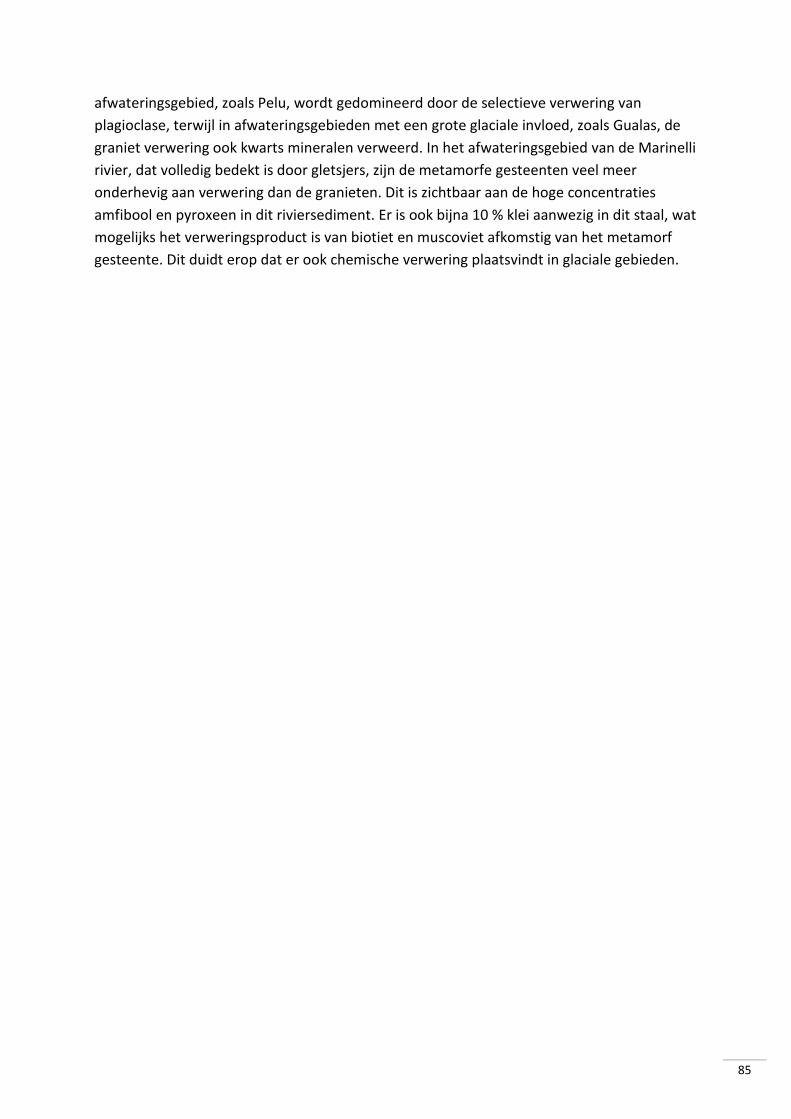
85
afwateringsgebied, zoals Pelu, wordt gedomineerd door de selectieve verwering van
plagioclase, terwijl in afwateringsgebieden met een grote glaciale invloed, zoals Gualas, de
graniet verwering ook kwarts mineralen verweerd. In het afwateringsgebied van de Marinelli
rivier, dat volledig bedekt is door gletsjers, zijn de metamorfe gesteenten veel meer
onderhevig aan verwering dan de granieten. Dit is zichtbaar aan de hoge concentraties
amfibool en pyroxeen in dit riviersediment. Er is ook bijna 10 % klei aanwezig in dit staal, wat
mogelijks het verweringsproduct is van biotiet en muscoviet afkomstig van het metamorf
gesteente. Dit duidt erop dat er ook chemische verwering plaatsvindt in glaciale gebieden.
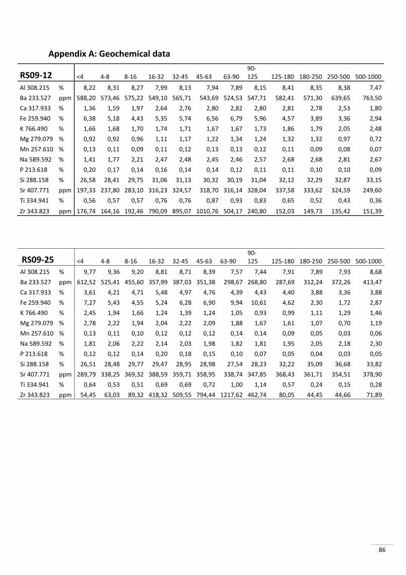
86
Appendix A: Geochemical data
RS09-12 <4 4-8 8-16 16-32 32-45 45-63 63-90 90-125 125-180 180-250 250-500 500-1000
Al 308.215 % 8,22 8,31 8,27 7,99 8,13 7,94 7,89 8,15 8,41 8,35 8,38 7,47
Ba 233.527 ppm 588,20 573,46 575,22 549,10 565,71 543,69 524,53 547,71 582,41 571,30 639,65 763,50
Ca 317.933 % 1,36 1,59 1,97 2,64 2,76 2,80 2,82 2,80 2,81 2,78 2,53 1,80
Fe 259.940 % 6,38 5,18 4,43 5,35 5,74 6,56 6,79 5,96 4,57 3,89 3,36 2,94
K 766.490 % 1,66 1,68 1,70 1,74 1,71 1,67 1,67 1,73 1,86 1,79 2,05 2,48
Mg 279.079 % 0,92 0,92 0,96 1,11 1,17 1,22 1,34 1,24 1,32 1,32 0,97 0,72
Mn 257.610 % 0,13 0,11 0,09 0,11 0,12 0,13 0,13 0,12 0,11 0,09 0,08 0,07
Na 589.592 % 1,41 1,77 2,21 2,47 2,48 2,45 2,46 2,57 2,68 2,68 2,81 2,67
P 213.618 % 0,20 0,17 0,14 0,16 0,14 0,14 0,12 0,11 0,11 0,10 0,10 0,09
Si 288.158 % 26,58 28,41 29,75 31,06 31,13 30,32 30,19 31,04 32,12 32,29 32,87 33,15
Sr 407.771 ppm 197,33 237,80 283,10 316,23 324,57 318,70 316,14 328,04 337,58 333,62 324,59 249,60
Ti 334.941 % 0,56 0,57 0,57 0,76 0,76 0,87 0,93 0,83 0,65 0,52 0,43 0,36
Zr 343.823 ppm 176,74 164,16 192,46 790,09 895,07 1010,76 504,17 240,80 152,03 149,73 135,42 151,39
RS09-25 <4 4-8 8-16 16-32 32-45 45-63 63-90 90-125 125-180 180-250 250-500 500-1000
Al 308.215 % 9,77 9,36 9,20 8,81 8,71 8,39 7,57 7,44 7,91 7,89 7,93 8,68
Ba 233.527 ppm 612,52 525,41 455,60 357,99 387,03 351,38 298,67 268,80 287,69 312,24 372,26 413,47
Ca 317.933 % 3,61 4,21 4,71 5,48 4,97 4,76 4,39 4,43 4,40 3,88 3,36 3,88
Fe 259.940 % 7,27 5,43 4,55 5,24 6,28 6,90 9,94 10,61 4,62 2,30 1,72 2,87
K 766.490 % 2,45 1,94 1,66 1,24 1,39 1,24 1,05 0,93 0,99 1,11 1,29 1,46
Mg 279.079 % 2,78 2,22 1,94 2,04 2,22 2,09 1,88 1,67 1,61 1,07 0,70 1,19
Mn 257.610 % 0,13 0,11 0,10 0,12 0,12 0,12 0,14 0,14 0,09 0,05 0,03 0,06
Na 589.592 % 1,81 2,06 2,22 2,14 2,03 1,98 1,82 1,81 1,95 2,05 2,18 2,30
P 213.618 % 0,12 0,12 0,14 0,20 0,18 0,15 0,10 0,07 0,05 0,04 0,03 0,05
Si 288.158 % 26,51 28,48 29,77 29,47 28,95 28,98 27,54 28,23 32,22 35,09 36,68 33,82
Sr 407.771 ppm 289,79 338,25 369,32 388,59 359,71 358,95 338,74 347,85 368,43 361,71 354,51 378,90
Ti 334.941 % 0,64 0,53 0,51 0,69 0,69 0,72 1,00 1,14 0,57 0,24 0,15 0,28
Zr 343.823 ppm 54,45 63,03 89,32 418,32 509,55 794,44 1217,62 462,74 80,05 44,45 44,66 71,89
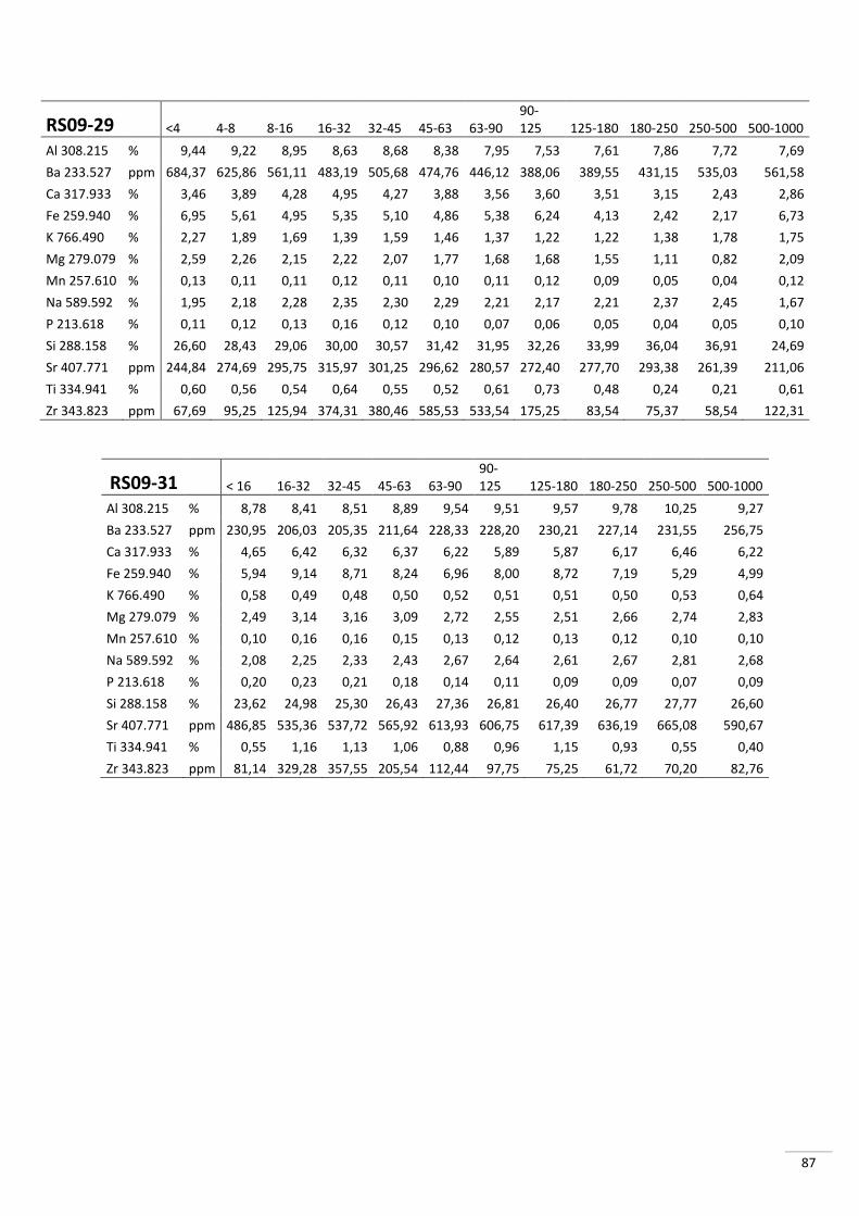
87
RS09-29 <4 4-8 8-16 16-32 32-45 45-63 63-90 90-125 125-180 180-250 250-500 500-1000
Al 308.215 % 9,44 9,22 8,95 8,63 8,68 8,38 7,95 7,53 7,61 7,86 7,72 7,69
Ba 233.527 ppm 684,37 625,86 561,11 483,19 505,68 474,76 446,12 388,06 389,55 431,15 535,03 561,58
Ca 317.933 % 3,46 3,89 4,28 4,95 4,27 3,88 3,56 3,60 3,51 3,15 2,43 2,86
Fe 259.940 % 6,95 5,61 4,95 5,35 5,10 4,86 5,38 6,24 4,13 2,42 2,17 6,73
K 766.490 % 2,27 1,89 1,69 1,39 1,59 1,46 1,37 1,22 1,22 1,38 1,78 1,75
Mg 279.079 % 2,59 2,26 2,15 2,22 2,07 1,77 1,68 1,68 1,55 1,11 0,82 2,09
Mn 257.610 % 0,13 0,11 0,11 0,12 0,11 0,10 0,11 0,12 0,09 0,05 0,04 0,12
Na 589.592 % 1,95 2,18 2,28 2,35 2,30 2,29 2,21 2,17 2,21 2,37 2,45 1,67
P 213.618 % 0,11 0,12 0,13 0,16 0,12 0,10 0,07 0,06 0,05 0,04 0,05 0,10
Si 288.158 % 26,60 28,43 29,06 30,00 30,57 31,42 31,95 32,26 33,99 36,04 36,91 24,69
Sr 407.771 ppm 244,84 274,69 295,75 315,97 301,25 296,62 280,57 272,40 277,70 293,38 261,39 211,06
Ti 334.941 % 0,60 0,56 0,54 0,64 0,55 0,52 0,61 0,73 0,48 0,24 0,21 0,61
Zr 343.823 ppm 67,69 95,25 125,94 374,31 380,46 585,53 533,54 175,25 83,54 75,37 58,54 122,31
RS09-31 < 16 16-32 32-45 45-63 63-90 90-125 125-180 180-250 250-500 500-1000
Al 308.215 % 8,78 8,41 8,51 8,89 9,54 9,51 9,57 9,78 10,25 9,27
Ba 233.527 ppm 230,95 206,03 205,35 211,64 228,33 228,20 230,21 227,14 231,55 256,75
Ca 317.933 % 4,65 6,42 6,32 6,37 6,22 5,89 5,87 6,17 6,46 6,22
Fe 259.940 % 5,94 9,14 8,71 8,24 6,96 8,00 8,72 7,19 5,29 4,99
K 766.490 % 0,58 0,49 0,48 0,50 0,52 0,51 0,51 0,50 0,53 0,64
Mg 279.079 % 2,49 3,14 3,16 3,09 2,72 2,55 2,51 2,66 2,74 2,83
Mn 257.610 % 0,10 0,16 0,16 0,15 0,13 0,12 0,13 0,12 0,10 0,10
Na 589.592 % 2,08 2,25 2,33 2,43 2,67 2,64 2,61 2,67 2,81 2,68
P 213.618 % 0,20 0,23 0,21 0,18 0,14 0,11 0,09 0,09 0,07 0,09
Si 288.158 % 23,62 24,98 25,30 26,43 27,36 26,81 26,40 26,77 27,77 26,60
Sr 407.771 ppm 486,85 535,36 537,72 565,92 613,93 606,75 617,39 636,19 665,08 590,67
Ti 334.941 % 0,55 1,16 1,13 1,06 0,88 0,96 1,15 0,93 0,55 0,40
Zr 343.823 ppm 81,14 329,28 357,55 205,54 112,44 97,75 75,25 61,72 70,20 82,76

88
RS09-36 <4 4-8 8-16 16-32 32-45 45-63 63-90 90-125 125-180 180-250 250-500 500-1000
Al 308.215 % 7,50 7,27 7,01 6,28 6,69 6,06 6,28 6,45 6,63 6,89 6,88 6,77
Ba 233.527 ppm 402,89 344,56 304,26 252,70 296,37 282,73 310,54 327,71 368,09 436,74 438,37 368,06
Ca 317.933 % 7,77 9,00 9,15 8,96 8,97 8,28 8,39 8,12 7,63 6,64 6,61 6,87
Fe 259.940 % 8,58 7,82 8,01 11,04 9,88 10,83 9,79 7,59 6,50 5,18 5,21 5,65
K 766.490 % 0,97 0,81 0,73 0,64 0,74 0,77 0,81 0,86 0,98 1,11 1,18 1,03
Mg 279.079 % 5,59 5,58 5,35 5,13 5,35 4,70 4,83 4,47 4,04 3,36 3,36 3,72
Mn 257.610 % 0,14 0,14 0,14 0,15 0,15 0,14 0,14 0,12 0,11 0,08 0,08 0,10
Na 589.592 % 1,11 1,27 1,36 1,28 1,24 1,27 1,32 1,44 1,55 1,65 1,56 1,44
P 213.618 % 0,22 0,24 0,23 0,23 0,23 0,19 0,17 0,13 0,09 0,08 0,08 0,11
Si 288.158 % 21,76 23,04 23,25 22,28 22,70 23,57 24,72 26,67 27,70 29,19 28,04 25,35
Sr 407.771 ppm 531,83 596,71 605,32 557,24 568,18 532,75 564,28 601,03 645,24 672,77 641,98 585,67
Ti 334.941 % 0,96 1,04 1,02 1,02 1,02 0,84 0,80 0,66 0,56 0,47 0,46 0,51
Zr 343.823 ppm 67,03 78,51 88,03 107,27 92,08 113,18 100,24 50,24 51,58 46,79 52,37 59,35
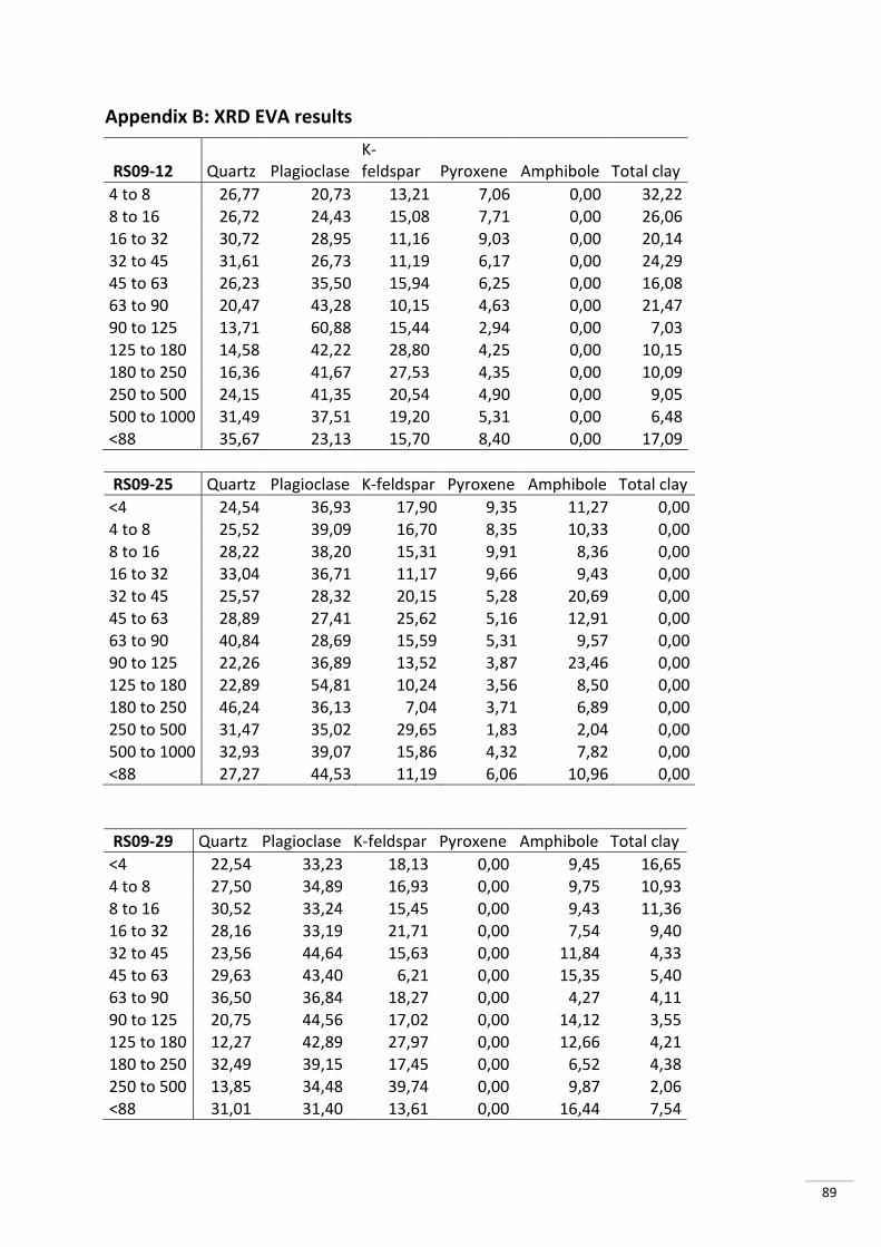
89
Appendix B: XRD EVA results
RS09-12 Quartz Plagioclase K-feldspar Pyroxene Amphibole Total clay
4 to 8 26,77 20,73 13,21 7,06 0,00 32,22 8 to 16 26,72 24,43 15,08 7,71 0,00 26,06 16 to 32 30,72 28,95 11,16 9,03 0,00 20,14 32 to 45 31,61 26,73 11,19 6,17 0,00 24,29 45 to 63 26,23 35,50 15,94 6,25 0,00 16,08 63 to 90 20,47 43,28 10,15 4,63 0,00 21,47 90 to 125 13,71 60,88 15,44 2,94 0,00 7,03 125 to 180 14,58 42,22 28,80 4,25 0,00 10,15
180 to 250 16,36 41,67 27,53 4,35 0,00 10,09 250 to 500 24,15 41,35 20,54 4,90 0,00 9,05 500 to 1000 31,49 37,51 19,20 5,31 0,00 6,48 <88 35,67 23,13 15,70 8,40 0,00 17,09
RS09-25 Quartz Plagioclase K-feldspar Pyroxene Amphibole Total clay
<4 24,54 36,93 17,90 9,35 11,27 0,00 4 to 8 25,52 39,09 16,70 8,35 10,33 0,00 8 to 16 28,22 38,20 15,31 9,91 8,36 0,00 16 to 32 33,04 36,71 11,17 9,66 9,43 0,00
32 to 45 25,57 28,32 20,15 5,28 20,69 0,00 45 to 63 28,89 27,41 25,62 5,16 12,91 0,00 63 to 90 40,84 28,69 15,59 5,31 9,57 0,00 90 to 125 22,26 36,89 13,52 3,87 23,46 0,00 125 to 180 22,89 54,81 10,24 3,56 8,50 0,00 180 to 250 46,24 36,13 7,04 3,71 6,89 0,00 250 to 500 31,47 35,02 29,65 1,83 2,04 0,00 500 to 1000 32,93 39,07 15,86 4,32 7,82 0,00 <88 27,27 44,53 11,19 6,06 10,96 0,00
RS09-29 Quartz Plagioclase K-feldspar Pyroxene Amphibole Total clay
<4 22,54 33,23 18,13 0,00 9,45 16,65 4 to 8 27,50 34,89 16,93 0,00 9,75 10,93 8 to 16 30,52 33,24 15,45 0,00 9,43 11,36 16 to 32 28,16 33,19 21,71 0,00 7,54 9,40 32 to 45 23,56 44,64 15,63 0,00 11,84 4,33 45 to 63 29,63 43,40 6,21 0,00 15,35 5,40 63 to 90 36,50 36,84 18,27 0,00 4,27 4,11 90 to 125 20,75 44,56 17,02 0,00 14,12 3,55 125 to 180 12,27 42,89 27,97 0,00 12,66 4,21 180 to 250 32,49 39,15 17,45 0,00 6,52 4,38
250 to 500 13,85 34,48 39,74 0,00 9,87 2,06 <88 31,01 31,40 13,61 0,00 16,44 7,54
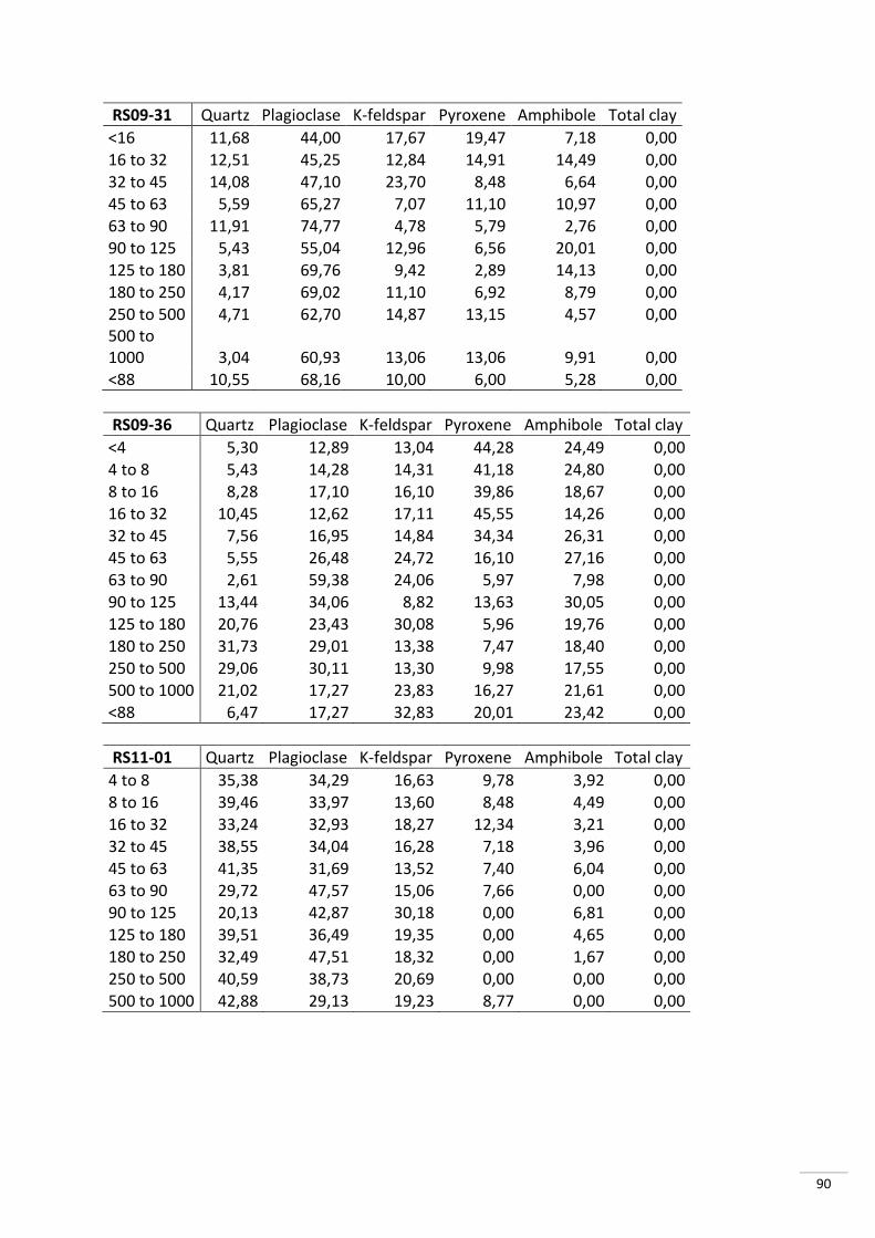
90
RS09-31 Quartz Plagioclase K-feldspar Pyroxene Amphibole Total clay
<16 11,68 44,00 17,67 19,47 7,18 0,00 16 to 32 12,51 45,25 12,84 14,91 14,49 0,00 32 to 45 14,08 47,10 23,70 8,48 6,64 0,00 45 to 63 5,59 65,27 7,07 11,10 10,97 0,00 63 to 90 11,91 74,77 4,78 5,79 2,76 0,00 90 to 125 5,43 55,04 12,96 6,56 20,01 0,00 125 to 180 3,81 69,76 9,42 2,89 14,13 0,00 180 to 250 4,17 69,02 11,10 6,92 8,79 0,00 250 to 500 4,71 62,70 14,87 13,15 4,57 0,00 500 to 1000 3,04 60,93 13,06 13,06 9,91 0,00 <88 10,55 68,16 10,00 6,00 5,28 0,00
RS09-36 Quartz Plagioclase K-feldspar Pyroxene Amphibole Total clay
<4 5,30 12,89 13,04 44,28 24,49 0,00 4 to 8 5,43 14,28 14,31 41,18 24,80 0,00 8 to 16 8,28 17,10 16,10 39,86 18,67 0,00 16 to 32 10,45 12,62 17,11 45,55 14,26 0,00 32 to 45 7,56 16,95 14,84 34,34 26,31 0,00 45 to 63 5,55 26,48 24,72 16,10 27,16 0,00 63 to 90 2,61 59,38 24,06 5,97 7,98 0,00
90 to 125 13,44 34,06 8,82 13,63 30,05 0,00 125 to 180 20,76 23,43 30,08 5,96 19,76 0,00 180 to 250 31,73 29,01 13,38 7,47 18,40 0,00 250 to 500 29,06 30,11 13,30 9,98 17,55 0,00 500 to 1000 21,02 17,27 23,83 16,27 21,61 0,00 <88 6,47 17,27 32,83 20,01 23,42 0,00
RS11-01 Quartz Plagioclase K-feldspar Pyroxene Amphibole Total clay
4 to 8 35,38 34,29 16,63 9,78 3,92 0,00 8 to 16 39,46 33,97 13,60 8,48 4,49 0,00
16 to 32 33,24 32,93 18,27 12,34 3,21 0,00 32 to 45 38,55 34,04 16,28 7,18 3,96 0,00 45 to 63 41,35 31,69 13,52 7,40 6,04 0,00 63 to 90 29,72 47,57 15,06 7,66 0,00 0,00 90 to 125 20,13 42,87 30,18 0,00 6,81 0,00 125 to 180 39,51 36,49 19,35 0,00 4,65 0,00 180 to 250 32,49 47,51 18,32 0,00 1,67 0,00 250 to 500 40,59 38,73 20,69 0,00 0,00 0,00 500 to 1000 42,88 29,13 19,23 8,77 0,00 0,00
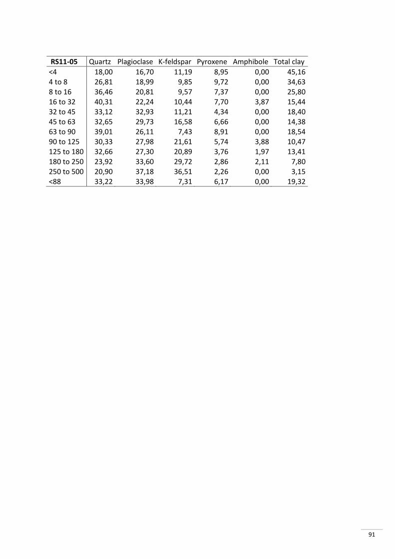
91
RS11-05 Quartz Plagioclase K-feldspar Pyroxene Amphibole Total clay
<4 18,00 16,70 11,19 8,95 0,00 45,16 4 to 8 26,81 18,99 9,85 9,72 0,00 34,63 8 to 16 36,46 20,81 9,57 7,37 0,00 25,80 16 to 32 40,31 22,24 10,44 7,70 3,87 15,44 32 to 45 33,12 32,93 11,21 4,34 0,00 18,40 45 to 63 32,65 29,73 16,58 6,66 0,00 14,38 63 to 90 39,01 26,11 7,43 8,91 0,00 18,54 90 to 125 30,33 27,98 21,61 5,74 3,88 10,47 125 to 180 32,66 27,30 20,89 3,76 1,97 13,41
180 to 250 23,92 33,60 29,72 2,86 2,11 7,80 250 to 500 20,90 37,18 36,51 2,26 0,00 3,15 <88 33,22 33,98 7,31 6,17 0,00 19,32
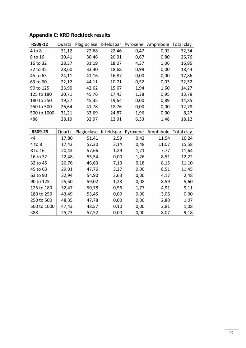
92
Appendix C: XRD RockJock results
RS09-12 Quartz Plagioclase K-feldspar Pyroxene Amphibole Total clay
4 to 8 21,12 22,68 22,46 0,47 0,92 32,34 8 to 16 20,41 30,46 20,91 0,67 0,80 26,76 16 to 32 28,37 31,19 18,07 4,37 1,06 16,95 32 to 45 28,60 33,30 18,68 0,98 0,00 18,44 45 to 63 24,11 41,16 16,87 0,00 0,00 17,86 63 to 90 22,12 44,11 10,71 0,52 0,03 22,52 90 to 125 23,90 42,62 15,67 1,94 1,60 14,27 125 to 180 20,71 45,76 17,43 1,38 0,95 13,78
180 to 250 19,27 45,35 19,64 0,00 0,89 14,85 250 to 500 26,64 41,78 18,76 0,00 0,00 12,78 500 to 1000 31,21 33,69 24,87 1,96 0,00 8,27 <88 28,19 32,97 12,91 6,33 1,48 18,12
RS09-25 Quartz Plagioclase K-feldspar Pyroxene Amphibole Total clay
<4 17,80 51,41 2,59 0,42 11,54 16,24 4 to 8 17,43 52,30 3,14 0,48 11,07 15,58 8 to 16 20,43 57,66 1,29 1,21 7,77 11,64 16 to 32 22,48 55,54 0,00 1,26 8,51 12,22 32 to 45 26,76 46,63 7,19 0,18 8,15 11,10
45 to 63 29,01 47,76 3,27 0,00 8,51 11,45 63 to 90 32,94 54,90 3,63 0,00 4,17 2,48 90 to 125 25,50 59,02 1,23 0,08 8,59 5,60 125 to 180 32,47 50,78 0,96 1,77 4,91 9,11 180 to 250 43,49 53,45 0,00 0,00 3,06 0,00 250 to 500 48,35 47,78 0,00 0,00 2,80 1,07 500 to 1000 47,43 48,57 0,10 0,00 2,81 1,08 <88 25,23 57,52 0,00 0,00 8,07 9,18
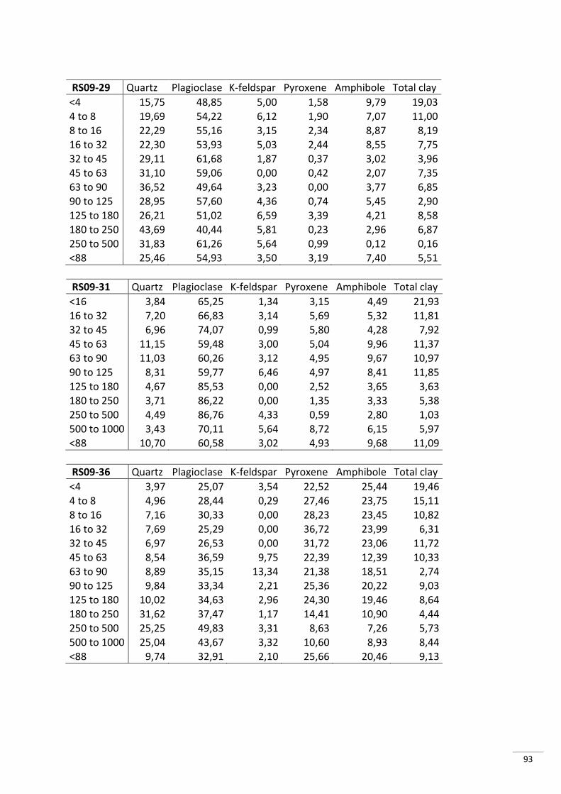
93
RS09-29 Quartz Plagioclase K-feldspar Pyroxene Amphibole Total clay
<4 15,75 48,85 5,00 1,58 9,79 19,03 4 to 8 19,69 54,22 6,12 1,90 7,07 11,00 8 to 16 22,29 55,16 3,15 2,34 8,87 8,19 16 to 32 22,30 53,93 5,03 2,44 8,55 7,75 32 to 45 29,11 61,68 1,87 0,37 3,02 3,96 45 to 63 31,10 59,06 0,00 0,42 2,07 7,35 63 to 90 36,52 49,64 3,23 0,00 3,77 6,85 90 to 125 28,95 57,60 4,36 0,74 5,45 2,90 125 to 180 26,21 51,02 6,59 3,39 4,21 8,58
180 to 250 43,69 40,44 5,81 0,23 2,96 6,87 250 to 500 31,83 61,26 5,64 0,99 0,12 0,16 <88 25,46 54,93 3,50 3,19 7,40 5,51
RS09-31 Quartz Plagioclase K-feldspar Pyroxene Amphibole Total clay
<16 3,84 65,25 1,34 3,15 4,49 21,93 16 to 32 7,20 66,83 3,14 5,69 5,32 11,81 32 to 45 6,96 74,07 0,99 5,80 4,28 7,92 45 to 63 11,15 59,48 3,00 5,04 9,96 11,37 63 to 90 11,03 60,26 3,12 4,95 9,67 10,97 90 to 125 8,31 59,77 6,46 4,97 8,41 11,85
125 to 180 4,67 85,53 0,00 2,52 3,65 3,63 180 to 250 3,71 86,22 0,00 1,35 3,33 5,38 250 to 500 4,49 86,76 4,33 0,59 2,80 1,03 500 to 1000 3,43 70,11 5,64 8,72 6,15 5,97 <88 10,70 60,58 3,02 4,93 9,68 11,09
RS09-36 Quartz Plagioclase K-feldspar Pyroxene Amphibole Total clay
<4 3,97 25,07 3,54 22,52 25,44 19,46 4 to 8 4,96 28,44 0,29 27,46 23,75 15,11 8 to 16 7,16 30,33 0,00 28,23 23,45 10,82
16 to 32 7,69 25,29 0,00 36,72 23,99 6,31 32 to 45 6,97 26,53 0,00 31,72 23,06 11,72 45 to 63 8,54 36,59 9,75 22,39 12,39 10,33 63 to 90 8,89 35,15 13,34 21,38 18,51 2,74 90 to 125 9,84 33,34 2,21 25,36 20,22 9,03 125 to 180 10,02 34,63 2,96 24,30 19,46 8,64 180 to 250 31,62 37,47 1,17 14,41 10,90 4,44 250 to 500 25,25 49,83 3,31 8,63 7,26 5,73 500 to 1000 25,04 43,67 3,32 10,60 8,93 8,44 <88 9,74 32,91 2,10 25,66 20,46 9,13
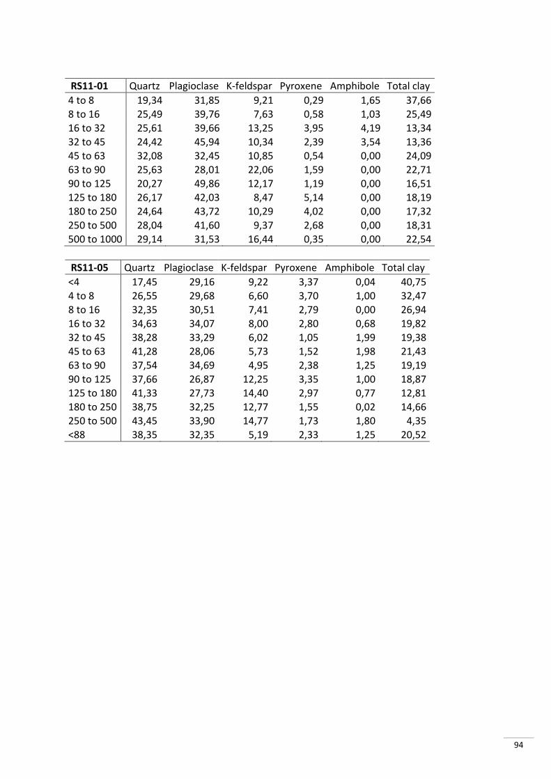
94
RS11-01 Quartz Plagioclase K-feldspar Pyroxene Amphibole Total clay
4 to 8 19,34 31,85 9,21 0,29 1,65 37,66 8 to 16 25,49 39,76 7,63 0,58 1,03 25,49 16 to 32 25,61 39,66 13,25 3,95 4,19 13,34 32 to 45 24,42 45,94 10,34 2,39 3,54 13,36 45 to 63 32,08 32,45 10,85 0,54 0,00 24,09 63 to 90 25,63 28,01 22,06 1,59 0,00 22,71 90 to 125 20,27 49,86 12,17 1,19 0,00 16,51 125 to 180 26,17 42,03 8,47 5,14 0,00 18,19 180 to 250 24,64 43,72 10,29 4,02 0,00 17,32
250 to 500 28,04 41,60 9,37 2,68 0,00 18,31 500 to 1000 29,14 31,53 16,44 0,35 0,00 22,54
RS11-05 Quartz Plagioclase K-feldspar Pyroxene Amphibole Total clay
<4 17,45 29,16 9,22 3,37 0,04 40,75 4 to 8 26,55 29,68 6,60 3,70 1,00 32,47 8 to 16 32,35 30,51 7,41 2,79 0,00 26,94 16 to 32 34,63 34,07 8,00 2,80 0,68 19,82 32 to 45 38,28 33,29 6,02 1,05 1,99 19,38 45 to 63 41,28 28,06 5,73 1,52 1,98 21,43 63 to 90 37,54 34,69 4,95 2,38 1,25 19,19
90 to 125 37,66 26,87 12,25 3,35 1,00 18,87 125 to 180 41,33 27,73 14,40 2,97 0,77 12,81 180 to 250 38,75 32,25 12,77 1,55 0,02 14,66 250 to 500 43,45 33,90 14,77 1,73 1,80 4,35 <88 38,35 32,35 5,19 2,33 1,25 20,52
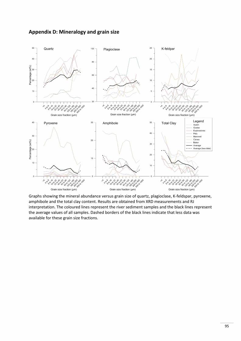
95
Appendix D: Mineralogy and grain size
Graphs showing the mineral abundance versus grain size of quartz, plagioclase, K-feldspar, pyroxene, amphibole and the total clay content. Results are obtained from XRD measurements and RJ interpretation. The coloured lines represent the river sediment samples and the black lines represent the average values of all samples. Dashed borders of the black lines indicate that less data was available for these grain size fractions.