Model-based predictive control of a batteryenergy storage for fast frequency control indistribution grids using load flow analysis

Modellpradiktive Regelung eines Batteriespeichers zurFrequenzstabilisierung in einem Verteilnetzabschnitt mittels

Lastflussanalyse

Master Thesis

submitted in partial fulfilment of the requirements for the degree ofMaster of Engineering

at the department Life Sciences of

Hamburg University of Applied Sciences (HAW Hamburg)

In cooperation withFraunhofer Institute for Silicon Technology (ISIT)

Supervisors:1. Dr.-Ing. Gerwald Lichtenberg (HAW Hamburg)

2. Dr.-Ing. Georg Pangalos (Fraunhofer ISIT)

Sascha Nadja RinglstetterMatriculation number:

Hamburg, 31. August 2017

Hereby I declare that I produced the present work myself only with the help of theindicated aids and sources.

Hamburg, 31. August 2017 Sascha Nadja Ringlstetter

Contents

1 Introduction 1

2 Electric distribution grids 2

2.1 Electric transmission and distribution networks . . . . . . . . . . . . . . . 2

2.1.1 Transmission grids . . . . . . . . . . . . . . . . . . . . . . . . . . . 2

2.1.2 Distribution grids . . . . . . . . . . . . . . . . . . . . . . . . . . . . 3

2.2 Single line AC load flow analysis . . . . . . . . . . . . . . . . . . . . . . . . 3

2.2.1 Principle . . . . . . . . . . . . . . . . . . . . . . . . . . . . . . . . . 4

2.2.2 Algorithm . . . . . . . . . . . . . . . . . . . . . . . . . . . . . . . . 5

2.2.3 Test feeder . . . . . . . . . . . . . . . . . . . . . . . . . . . . . . . . 6

2.2.4 Combining varying system frequency with load flow analysis . . . . 8

2.2.5 Comparison load flow and other electric network modelling approaches 9

2.3 Frequency deviation in electric networks . . . . . . . . . . . . . . . . . . . 10

2.3.1 Origin of frequency deviation, rotating masses . . . . . . . . . . . . 10

2.3.2 Different types of load frequency control . . . . . . . . . . . . . . . 13

2.3.3 Regulations for primary load frequency control . . . . . . . . . . . . 13

2.3.4 Dynamic load frequency response model . . . . . . . . . . . . . . . 16

2.4 Li-ion based battery energy storage . . . . . . . . . . . . . . . . . . . . . . 19

3 Model based predictive control 21

3.1 Model predictive control . . . . . . . . . . . . . . . . . . . . . . . . . . . . 21

3.1.1 Working principle . . . . . . . . . . . . . . . . . . . . . . . . . . . . 21

3.1.2 Optimisation of the objective function . . . . . . . . . . . . . . . . 23

3.2 Nelder-Mead simplex optimisation . . . . . . . . . . . . . . . . . . . . . . . 24

3.2.1 Nelder-Mead simplex algorithm . . . . . . . . . . . . . . . . . . . . 24

3.2.2 Optimisation with inequality constraints . . . . . . . . . . . . . . . 25

3.3 Golden section search optimisation . . . . . . . . . . . . . . . . . . . . . . 26

4 Modelling and control algorithm 27

4.1 Controller structure and algorithm . . . . . . . . . . . . . . . . . . . . . . 27

4.2 Network modelling . . . . . . . . . . . . . . . . . . . . . . . . . . . . . . . 29

4.2.1 Static electricity network model . . . . . . . . . . . . . . . . . . . . 30

4.2.2 Dynamic frequency deviation model . . . . . . . . . . . . . . . . . . 30

i

4.2.3 Battery storage model . . . . . . . . . . . . . . . . . . . . . . . . . 35

4.3 Demand data . . . . . . . . . . . . . . . . . . . . . . . . . . . . . . . . . . 37

4.3.1 Analysis of single phases and relationship of reactive to active power 38

4.3.2 Demand power analysis and prediction approaches . . . . . . . . . . 39

4.4 Objective function . . . . . . . . . . . . . . . . . . . . . . . . . . . . . . . 44

5 Simulation studies 47

5.1 Comparison of operating modes . . . . . . . . . . . . . . . . . . . . . . . . 47

5.2 Load data . . . . . . . . . . . . . . . . . . . . . . . . . . . . . . . . . . . . 48

5.3 Parameter variation . . . . . . . . . . . . . . . . . . . . . . . . . . . . . . . 48

5.4 Performance evaluation . . . . . . . . . . . . . . . . . . . . . . . . . . . . . 50

5.5 Results and analysis . . . . . . . . . . . . . . . . . . . . . . . . . . . . . . 50

5.5.1 System frequency without battery action . . . . . . . . . . . . . . . 51

5.5.2 Observed issues with different operating modes and optimisationalgorithms . . . . . . . . . . . . . . . . . . . . . . . . . . . . . . . . 51

5.5.3 Varying battery storage size . . . . . . . . . . . . . . . . . . . . . . 52

5.5.4 Varying simulation horizon . . . . . . . . . . . . . . . . . . . . . . . 53

5.5.5 Varying battery delay time . . . . . . . . . . . . . . . . . . . . . . . 54

5.5.6 Result figures . . . . . . . . . . . . . . . . . . . . . . . . . . . . . . 55

6 Conclusion and Outlook 64

6.1 Conclusion . . . . . . . . . . . . . . . . . . . . . . . . . . . . . . . . . . . . 64

6.2 Outlook . . . . . . . . . . . . . . . . . . . . . . . . . . . . . . . . . . . . . 64

ii

1 Introduction

This thesis proposes a model-based predictive control algorithm for a Li-ion based BatteryEnergy Storage System (BESS) using load flow computations. It should be examined ifsuch a controller can show improved performance in stabilising the frequency in a distri-bution grid compared to current load frequency control services. A continuous controlalgorithm was developed in Matlab environment combining different concepts that are de-scribed in the following. A simulation study was conducted for evaluating the controllerbehaviour and for comparing it with other operating modes.

Deviations of the system frequency from its set point value in electric networks resultfrom imbalances between generated and consumed energy. Such can be sudden changesin demand power that are compensated by conventional generation units with rotatingmasses. In real networks, frequency deviations are tackled by primary and secondaryLoad Frequency Control (LFC) units. They react to measured frequency deviations byproportionally injecting or absorbing active power into or from the grid.The proposed battery control algorithm is based on active power measurements at strate-gic points of the electricity grid, which are assumed to be obtained faster than frequencymeasurements. Based on the observed changes in system loads, future frequency devia-tions are predicted in short-term range. This allows the computation of a battery signalthat efficiently reduces the expected frequency deviation.With the motivation of increasing the speed of the control algorithm, load flow analysistechniques were applied for calculating line and transformer losses in the power grid. Asimplified model of the distribution grid was used for determining the active and reactivepower losses, required active and reactive power of connected generators, as well as volt-age magnitudes and angles at all buses of a steady-state operated electric network. Thegrid structure was assumed to be similar to an island grid, with one coupling point tothe transmission grid that is represented by a synchronous generator. The prediction offuture frequency deviation was based on a dynamic model of a conventional reheat-steamturbine. A BESS connected to the power system was modelled for partly compensatingsmall load changes and thus helping to reduce future frequency deviations. The optimalsequence of active power provided by the battery storage should be determined with adownhill simplex optimisation algorithm.

In the following document, chapters 2 and 3 comprise introductions into the underlyingtheoretical concepts of network analysis and model-based predictive control. The modelsapplied in the proposes controller structure are explained in chapter 4. Chapter 5 presentsthe approach, results and analysis of the simulation study. Finally, chapter 6 summarisesthe main conclusions drawn and gives some proposals for future work.

1

2 Electric distribution grids

This chapter will give an overview of the theoretical background and modelling conceptsfor electric distribution networks that were applied in the proposed battery controller.They include static network calculation, dynamic modelling of expected frequency devi-ations, and an introduction to applications of large scale Li-ion based battery storages inelectrical networks.

2.1 Electric transmission and distribution networks

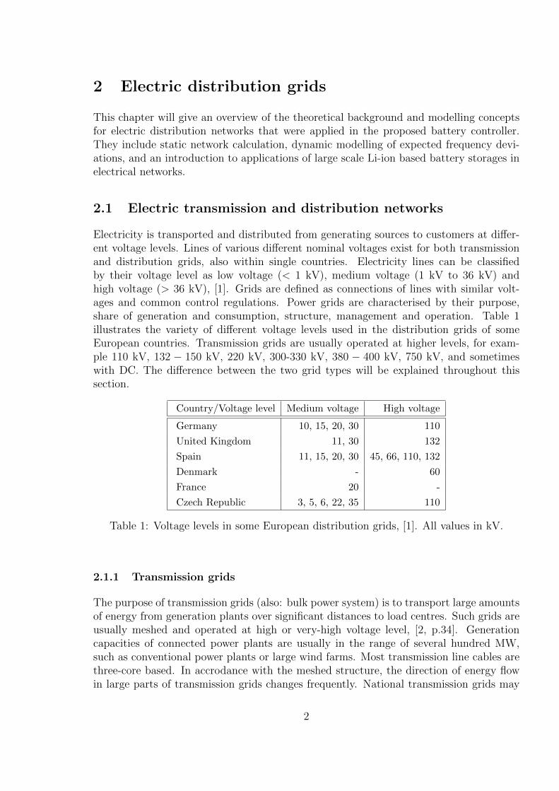
Electricity is transported and distributed from generating sources to customers at differ-ent voltage levels. Lines of various different nominal voltages exist for both transmissionand distribution grids, also within single countries. Electricity lines can be classifiedby their voltage level as low voltage (< 1 kV), medium voltage (1 kV to 36 kV) andhigh voltage (> 36 kV), [1]. Grids are defined as connections of lines with similar volt-ages and common control regulations. Power grids are characterised by their purpose,share of generation and consumption, structure, management and operation. Table 1illustrates the variety of different voltage levels used in the distribution grids of someEuropean countries. Transmission grids are usually operated at higher levels, for exam-ple 110 kV, 132 − 150 kV, 220 kV, 300-330 kV, 380 − 400 kV, 750 kV, and sometimeswith DC. The difference between the two grid types will be explained throughout thissection.

Country/Voltage level Medium voltage High voltage

Germany 10, 15, 20, 30 110

United Kingdom 11, 30 132

Spain 11, 15, 20, 30 45, 66, 110, 132

Denmark - 60

France 20 -

Czech Republic 3, 5, 6, 22, 35 110

Table 1: Voltage levels in some European distribution grids, [1]. All values in kV.

2.1.1 Transmission grids

The purpose of transmission grids (also: bulk power system) is to transport large amountsof energy from generation plants over significant distances to load centres. Such grids areusually meshed and operated at high or very-high voltage level, [2, p.34]. Generationcapacities of connected power plants are usually in the range of several hundred MW,such as conventional power plants or large wind farms. Most transmission line cables arethree-core based. In accrodance with the meshed structure, the direction of energy flowin large parts of transmission grids changes frequently. National transmission grids may

2

comprise several connected control areas. They are operated by Transmission SystemOperators (TSOs).In Germany, these are “TransnetBW GmbH”, “TenneT TSO GmbH”, “Amprion GmbH”and “50Hertz Transmission GmbH”.The regulations for the Continental European synchronously operated electricity trans-mission grid are issued by “ENTSO-E”, the European Network of Transmission SystemOperators for Electricity. It is an international association of European TSOs and the Eu-ropean Commissions reference body, [3]. Before 2009, the institution was named “UCTE”,Union for the Co-ordination of Transmission of Electricity. The main task of this associ-ation comprising 43 TSOs from 36 European countries is to coordinate the operation anddevelopment of the synchronised connected European electricity transmission grid. TheContinental European synchronously operated electricity transmission grid has a peakand off-peak design load of 300 GW and 150 GW, respectively, [4]. An interesting anddetailed online map of the European transmission grid can be found in [5]. The mon-itoring and real-time analysis systems of several European TSO’s is conducted by thetechnical coordination centre for Central West Europe “Coreso”.

2.1.2 Distribution grids

Via substations, the transmission grids are coupled to distribution grids. Within those,electric energy is transmitted to local networks with residential customers or other endusers such as industry, institutions, or small and medium enterprises (SMEs), [3]. Dis-tribution grids can be high, medium or low voltage-based, or a combination of severaldifferent voltage levels, as the name relates mainly to the grid functionality. While inmedium and high voltage distribution grids commonly three-core lines are used, in lowvoltage grids often four-wire cables are applied, [2, p.34f]. The grids are operated byDistribution System Operators (DSOs).Historically, the energy flow in the often radial networks is mono directional, which meansonly from the coupling point in the direction of consumers. However, increasing share ofdistributed (often renewable) electricity sources can lead to multi-directional, time-variantflow of electric energy.

2.2 Single line AC load flow analysis

Load flow (power flow) calculation is a well-established method for analysing large powersystems, [6, p. 4-7]. It is used for determining the operating characteristics of an electricnetwork under steady-state conditions. The system states are basically computed bysolving a set of non linear, continuously differentiable equations. Over the last decades, theconvergence and usability of the algorithm could be enhanced by including the Newton-Raphson method, sparse matrix programming, and numerical integration techniques. Aload flow analysis can form the base for further analyses of transmission or distributionnetworks, such as unit commitment, security assessment, optimal system operation, faultor stability analyses. The following sections will present the basic principle of the single

3

line load flow analysis of AC electric networks. Single line means means that the threephases of a natural system are represented by one single phase in its model.

2.2.1 Principle

In load flow calculation, the power network is modelled as a set of buses (nodes), whichare connected through transmission lines. All network elements are represented by sim-plified algebraic models that are comprised of equivalent inductance, capacitance andresistance, [6, p.7f][7, p.5f]. Such lumped-circuit models exist, for example, for con-necting lines and cables, transformers (on nominal and off-nominal tap ratio, in-phaseand phase-shifting), and shunt elements. Loads and generators are modelled as constantsources or sinks of active and reactive power.

The whole system is assumed to be in steady-state or quasi steady state operation, thelatter meaning that it can be regarded as steady state with sufficient accuracy. Hence,dynamic phenomena, such as electro-magnetic transients or small load changes are ne-glected. The system frequency and all voltages are assumed to be constant within oneload flow analysis [6][7]. The operating state of the system can be fully described byspecifying the following variables at each bus k in the system [7].

• Vk - voltage magnitude

• θk - voltage phase angle

• Pk - net active power (algebraic sum of generation and consumption)

• Qk - net reactive power

This corresponds to knowing the complex voltages and complex powers (active and reac-tive) absorbed or generated at all buses, leading to the complex power flows and lossesalong the connecting lines [6]. Usually, all variables are expressed in p.u. (per unit) valueswith respect to a system base.The following three basic types of buses are defined. At each of these, two variables aregiven beforehand and two unknowns have to be determined, [6, p.17][7, p.31f].

1. V θ slack bus (swing/reference bus): a selected voltage-controlled bus, whose volt-age phase angle is used as reference for the whole system. Its active and reactivepower injection will balance the system’s generations, loads and losses. Usually one(or multiple) generating station responsible for Load Frequency Control (LFC) isspecified as slack bus.

2. PQ nonvoltage-controlled bus (load bus): bus at which total injected powerPk + jQk is given. Buses of this type usually corresponds to consumers and formthe majority of buses in the system.

3. PV voltage-controlled bus: bus with fixed voltage magnitude and active powerinjection. They can represent a synchronous generator with voltage control or syn-chronous compensators injecting reactive power at substations.

4

2.2.2 Algorithm

This section presents the basic steps of load flow computation. In the nodal method,one nonlinear algebraic equation can be formulated for each bus of the system, based onKirchhoff’s Current Law. The equation for one node (bus)

Ik =∑m∈K

YkmEm (2.1)

=∑m∈K

(Gkm + jBkm)(Vmejθm), (2.2)

comprises the net current Ik of the respective node and complex voltages Ek = Vkejθk of

all adjacent nodes as variables (K : set of buses adjacent to k including k). Currents andvoltages are linked through line admittances Ykm = (Gkm + jBkm), [7, p.27ff][6, p.12ff][2,p.808ff]. The single equations are combined with the help of the system admittancematrix Y to

I = Y · E. (2.3)

With complex net power injection at each bus k : Sk = Pk + jQk = EkIk∗ , the activeand reactive power components can be calculated as

Pk = Vk∑m`K

Vm(Gkm cos θkm +Bkm sin θkm), (2.4)

Qk = Vk∑m`K

Vm(Gkm sin θkm −Bkm cos θkm), (2.5)

and the resulting system of equations is solved iteratively, [7].In order to reflect operating limits of generators and other network components (lines,transformers etc.), inequality constraints may be formulated. The consideration of suchlimits can be realized by transforming a bus into a different bus type when a constraint isviolated or by incrementally adjusting the bus variables until the constraints are satisfied.For iteratively solving the nonlinear equation system, a Newton-Raphson algorithm isapplied using linear approximations based on Taylor series expansion of first order, [6].In each iteration p, the updated variable

xp+1 = xp + ∆xp (2.6)

≈ xp − J−1(xp)f(xp) (2.7)

is computed based the estimate x(p) of the variable x. The Jacobian matrix J for nfunctions f = (f1(x), f2(x), ...fn(x))T with a vector of variables x = (x1, x2, ..., xn)T isconstructed from first-order partial differentials, such as Jkm = δfk

δxmfor fk(xm)). For the

load flow computation, with

x =

(θ

V

), (2.8)

f(x) =

(∆P(x)

∆Q(x)

)(2.9)

5

the Jacobian matrix

J =

(∂∆P∂θ

∂∆P∂V

∂∆Q∂θ

∂∆Q∂V

)(2.10)

=

(∂P∂θ

∂P∂V

∂Q∂θ

∂Q∂V

)(2.11)

can be formulated, based on (2.4) and (2.5), [6][8]. Hence the system of nonlinear equa-tions (

∆P(θ,V)

∆Q(θ,V)

)= J(θ,V)

(∆θ

∆V

)(2.12)

can be obtained. In each nodal equation, different variables are known or unknown ac-cording to the respective bus types, as defined in section 2.2.1. The main steps of initerative load flow computation are illustrated as a flow chart in figure 2.1. In this the-sis, a Matlab code for basic load flow computation based on Newton Raphson iterativemethod was used, which had been retrieved from Matlab file exchange, [9]. The computa-tional speed of load flow calculations can be further increased by the so-called decouplingmethod. In a certain range of θ around zero, the relationships P − V and Q − θ can beneglected, [10, p.45ff]. This corresponds to setting the following elements of the Jacobianmatrix to zero: δP/δV and δQ/δθ, leading to

Jdecoupled =

(∂P∂θ

0

0 ∂Q∂V

). (2.13)

By this, the dimension of the set of equations to be solved is reduced. The admittancematrix characterises the connections of all nodes of the network with each other. Depend-ing on how meshed the network is, this matrix usually shows a high degree of sparsity,allowing the application of special sparse matrix algorithms for storage and solving issues.By this, the computational speed can be further enhanced, [2, p.812].

2.2.3 Test feeder

The aim of test feeders is to provide benchmark systems for comparison and verificationof power system analysis methods and programmes, [11]. Such test feeders can have dif-ferent characteristics, such as being one- or three-phase based, radial or meshed, balancedor unbalanced. Test feeder data contain load data with specification of bus types andvariable values (e.g. active and reactive power for PQ-bus). Line data is given in formsof equivalent model data. Further information and operating limits may be given, suchas electrical (e.g. type of line: transformer, other) or geospatial data like length of thelines or location of the buses, and minimum/maximum voltage magnitudes, angles, powervalues. Usually all data is expressed in p.u. values, which enables using test feeders atvoltage levels different to the original version, and independently from the original systemfrequency.

6

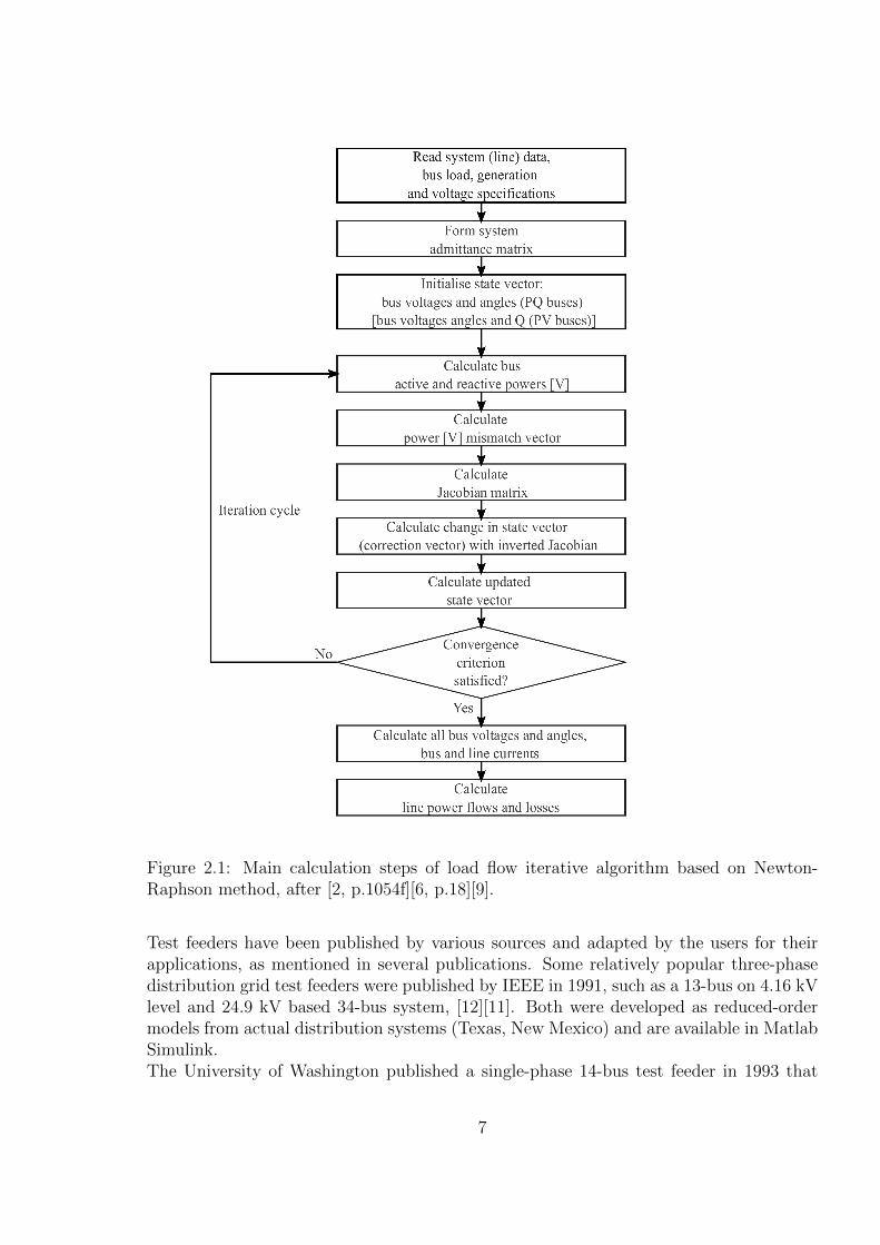
Figure 2.1: Main calculation steps of load flow iterative algorithm based on Newton-Raphson method, after [2, p.1054f][6, p.18][9].

Test feeders have been published by various sources and adapted by the users for theirapplications, as mentioned in several publications. Some relatively popular three-phasedistribution grid test feeders were published by IEEE in 1991, such as a 13-bus on 4.16 kVlevel and 24.9 kV based 34-bus system, [12][11]. Both were developed as reduced-ordermodels from actual distribution systems (Texas, New Mexico) and are available in MatlabSimulink.The University of Washington published a single-phase 14-bus test feeder in 1993 that

7

has been used in several publications, [13]. It is available in IEEE Common Data Format,and represents a simplified portion of a Midwestern American Electric Power System asof 1962.A set of single-phase test feeders published by the UK Centre for Sustainable Electricityand Distributed Generation (SEDG) in 2005 is representative of UK distribution net-works, [14]. The so-called “EHV1” model is a rural network test case on originally 33 kVlevel including long lines. It is fed from one 132 kV supply point. Due to a sub-sea cable,the test feeder shows voltage problems at the extremities of the system. It also containsa connection to another network. As this test feeder is both recent and representing anetwork similar to the aimed application of the battery storage, the “EHV1” test feederwas chosen as basis for the network models in this thesis. The feeder’s data and theofficial graphical scheme can be downloaded from [14].

2.2.4 Combining varying system frequency with load flow analysis

Generally, in load flow analysis steady-state conditions are assumed, including a constantsystem frequency. Though, in literature two different approaches can be found, which aimat combining frequency deviations resulting from load-generation imbalances with classicalload flow computations. In section 2.3, some theory on possible origins of frequencydeviations can be found.

Extended load flow (direct)In the first approach, presented by Okamura et.al. in the 70s [15] and used in [8]and [16][17], the deviation of system frequency from a rated frequency ∆f = f − fnomis directly included in the load flow algorithm. The deviation ∆f is incorporated intothe Newton-Raphson equations as additional state variable and is iteratively determinedduring computations. The respective elements of the extended Jacobian matrix

(∆P(θ,V,∆f)

∆Q(θ,V,∆f)

)= Jextended(θ,V,∆f)

∆θ

∆V

∆(∆f)

(2.14)

are derived from equations formulating the interaction of generators and frequency re-sponse as well as frequency-dependent loads. In order to maintain a solvable set of equa-tions (square matrices), ∆Pref may be introduced as additional variable on the left handside of the equation, representing the deviation of a generator bus from its referencevalue, [8].

Stepwise load flow (indirect)The approach of stepwise load flow is described by Bakken et.al. in [18]. In order to cal-culate slow power system dynamics of large networks with multiple generators, a sequenceof regular stationary AC load flows is combined with computation of frequency deviationfrom resulting power imbalance, based on droop response.The inputs to the algorithm are network topology data, information on amount, type andlimitations of available generation units. Starting from an initial state of the system, thestepwise power flow is executed recursively for changing loads, under the assumption that

8

scheduled generation usually is adjusted stepwise at the full change of hour, but demandis in-/ or decreasing linearly (also calculated stepwise, but at higher resolution). Theresulting power imbalance is used for calculating the frequency deviation by combineddroop settings of all connected generators. Based on the updated generator output pow-ers, the network operating state including all line flows, bus powers and complex voltages,are determined with a static load flow analysis.Besides the basic algorithm, the publication [18] presents further extensions, such as in-cluding distribution of generation among connected units, secondary reserve, cases ofgenerator or load outages, integration of wind power and economic aspects.

2.2.5 Comparison load flow and other electric network modelling approaches

Load flow analysis modelling of power systems is characterised by a high computationalspeed due to the included steady-state assumptions and significant simplification of theelectric network. However, with more detailed methods as described in following, it ispossible to describe further aspects of power grids more accurately.

A computationally demanding type, because very detailed, type of network analysis arefull electro-magnetic transient models (EMT). Herein, all instantaneous values of (sinu-soidal) voltages and currents are determined, [19, p.9]. They can include detailed passiveelements-representation of generators, transmission lines and loads. Such models areapplied for analysing time-variant dynamic behaviour of electric grids, for example oscil-latory behaviour of generators in case of short circuits or switching activities [2, p.851][6,p.245]. Due to the high computational demand, but ability to approximate short-timetime-variant transient effects well, EMT models are typically used for off-line computa-tion of small time frames, for example for design and coordination of transmission lineinsulation and equipment, [20].Another type of electric network simulations that had been derived from EMT models areso-called dynamic stability simulations (also: RMS simulations). They omit fast electro-magnetic transients in order to increase simulation speed. Dynamic stability simulationsare based on reduced order generator models and symmetric or unsymmetrical compo-nents methods, [19, p.9]. Possible applications are assessment of transient stability, faultride through, or dynamic behaviour of network components, [20].Additionally to the single-phase load flow presented and used in this work, power systemcan be studied using three-phase load flow. The method can be applied if electric grids arenot balanced, which means power flows of different magnitudes occur in the phases of thenetwork. This enables the assessment of unbalanced operation and detection of relatednegative effects on generators and transmission lines [6, p.42f]. Naturally, considerationof differences between phases requires more complex modelling and solving algorithmscompared to single-phase load flow, resulting in increased storage and computational re-quirements.

9

2.3 Frequency deviation in electric networks

In AC-based electric power networks, a common frequency can be observed throughoutthe whole system. It is named system frequency (mains frequency) and is a measure of therotational speed of all generators that are coupled and synchronised with the grid, [21].Within the ENTSO-E (European Network of Transmission System Operators) and neigh-bouring synchronized grids, the nominal value of system frequency is 50.0 Hz, [22]. Itmay be temporally changed to slightly different set point frequencies, for example forcorrection of the synchronous time.

2.3.1 Origin of frequency deviation, rotating masses

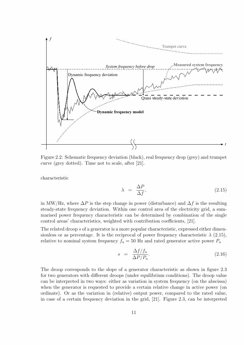
The actual system frequency can deviate from its set point value in case of imbalancesbetween net generated and consumed power. Such deviations are mainly related to activepower imbalances. Hence, they occur often at the change of the hour and during morning(sunrise) and evening (sunset) times, when the usually change faster than generation,[23][24]. Intermittent Renewable Energy Sources (RES) may add further variability ofactive power in the grid, however from the side of generating units. Frequency measure-ments are published online by many sources, commonly in intervals of seconds.Physically, deviations in system frequency result from synchronous generators, whoseturbine shafts are directly coupled to the grid. In case of disturbances of the demand-generation equilibrium, the additional positive or negative active power can be deliveredimmediately from the kinetic energy of the rotating masses (turbine shafts). This leadsto an increased or decreased rotational speed of the turbine shaft, which directly resultsin a change of system frequency. For example, a sudden increase in total demand powercan be compensated by a rotating mass of a conventional power plant, but at the expenseof a higher braking torque acting on the turbine shaft and slowing it down. Thus, thefrequency within the electric grid would drop, [2, p.728]. In conventional power plants,additionally to the kinetic energy of rotating masses, the change in requested generationpower is compensated by an increased use of primary energy. This is realised with acontroller aiming at restoring a constant rotational speed of the turbine shaft. Hence,after an initial frequency drop caused by the withdrawal of kinetic energy from rotatingmasses, the system frequency will be held at a constant value through primary governoraction. The remaining frequency deviation is called quasi-steady state deviation, [21].Both the governor unit and the turbine controller on which it is acting are characterisedby time constants of several seconds, causing delayed reaction. Figure 2.2 schematicallyillustrate the typical dynamic frequency response caused by primary control action of aconventional generation unit after a step change in load. Real measurements of frequencydrops can be assessed with enveloping trumpet curves. By this, the quality of secondarycontrol in the respective control areas can be evaluated, based on trumpet curve param-eter values obtained from frequency monitoring over several years, [21].

The relationship between load-generation imbalance and quasi-steady-state frequencydeviation is approximately proportional. It is described by the network power frequency

10

f

System frequency before drop Measured system frequency

Trumpet curve

t

Dynamic frequency deviation

Dynamic frequency model

Quasi steady-state deviation

Figure 2.2: Schematic frequency deviation (black), real frequency drop (grey) and trumpetcurve (grey dotted). Time not to scale, after [21].

characteristic

λ =∆P

∆f, (2.15)

in MW/Hz, where ∆P is the step change in power (disturbance) and ∆f is the resultingsteady-state frequency deviation. Within one control area of the electricity grid, a sum-marised power frequency characteristic can be determined by combination of the singlecontrol areas’ characteristics, weighted with contribution coefficients, [21].

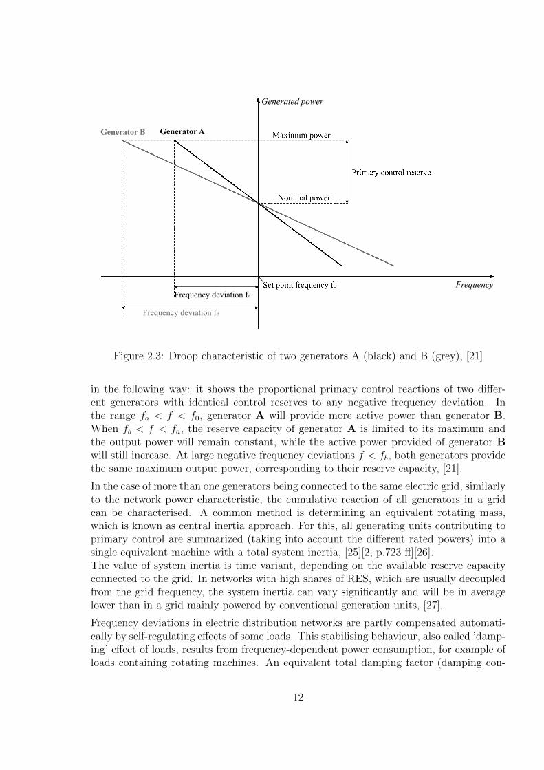
The related droop s of a generator is a more popular characteristic, expressed either dimen-sionless or as percentage. It is the reciprocal of power frequency characteristic λ (2.15),relative to nominal system frequency fn = 50 Hz and rated generator active power Pn

s =∆f/fn∆P/Pn

. (2.16)

The droop corresponds to the slope of a generator characteristic as shown in figure 2.3for two generators with different droops (under equilibrium conditions). The droop valuecan be interpreted in two ways: either as variation in system frequency (on the abscissa)when the generator is requested to provide a certain relative change in active power (onordinate). Or as the variation in (relative) output power, compared to the rated value,in case of a certain frequency deviation in the grid, [21]. Figure 2.3, can be interpreted

11

Generated power

FrequencyFrequency deviation fa

Generator B Generator A

Frequency deviation fb

Primary control reserve

Maximum power

Set point frequency f0

Nominal power

Figure 2.3: Droop characteristic of two generators A (black) and B (grey), [21]

in the following way: it shows the proportional primary control reactions of two differ-ent generators with identical control reserves to any negative frequency deviation. Inthe range fa < f < f0, generator A will provide more active power than generator B.When fb < f < fa, the reserve capacity of generator A is limited to its maximum andthe output power will remain constant, while the active power provided of generator Bwill still increase. At large negative frequency deviations f < fb, both generators providethe same maximum output power, corresponding to their reserve capacity, [21].

In the case of more than one generators being connected to the same electric grid, similarlyto the network power characteristic, the cumulative reaction of all generators in a gridcan be characterised. A common method is determining an equivalent rotating mass,which is known as central inertia approach. For this, all generating units contributing toprimary control are summarized (taking into account the different rated powers) into asingle equivalent machine with a total system inertia, [25][2, p.723 ff][26].The value of system inertia is time variant, depending on the available reserve capacityconnected to the grid. In networks with high shares of RES, which are usually decoupledfrom the grid frequency, the system inertia can vary significantly and will be in averagelower than in a grid mainly powered by conventional generation units, [27].

Frequency deviations in electric distribution networks are partly compensated automati-cally by self-regulating effects of some loads. This stabilising behaviour, also called ’damp-ing’ effect of loads, results from frequency-dependent power consumption, for example ofloads containing rotating machines. An equivalent total damping factor (damping con-

12

stant) can be used to describe the summarised self-regulating effect of the whole system.It is highly dependent on composition of active loads in every moment, [25][2, p.725][28,p.23].

2.3.2 Different types of load frequency control

Imbalances between generated and consumed power, and the resulting changes in systemfrequency, as described above, are commonly tackled by different control mechanisms.They are activated with different time lags.

• The primary control is the immediate compensation of active power imbalancesbetween load and generation. In electricity networks based on conventional powerplants, the connected turbines can restore the balance within a few seconds, based onspeed change of rotating masses speed and respective governor actions. Hereafter,the system frequency will remain at a fixed value, differing from the set-point value(steady-state deviation), [28, p.20]. The re-establishment of power balance canby supported by primary LFC services of other electricity sources. The reservecapacities in charge will be requested to deliver active power, proportionally to themeasured difference between set point and actual mains frequency, [21]. This helpsstabilising the frequency deviation at its steady-state value. Primary LFC is fullyactivated latest after 30 s and following will be decreased to zero within 15 min.

• The purpose of secondary control is to eliminate the constant frequency devia-tion caused by primary control of rotating masses in conventional generators whileensuring the equilibrium between generated and consumed active power. Throughcontrary power action, generators in charge will steer the mains frequency back to itsset point value. Secondary control is principally implemented as integral controllerwithin the contributing generating units, [2, p.727 ff][28]. It takes over from primaryfrequency control after some minutes and will be inactivated after 15 min, [21].

• In case of larger or longer disturbances, tertiary and emergency control maybe required in order to restore operating conditions after outages, [28, p.20][21]. Itcan be realised in manual or automatic way. In some literature sources, tertiarycontrol is referred to as the most economic dispatch of generation sources accordingto merit order principle, [2, p.728].

2.3.3 Regulations for primary load frequency control

Continental European synchronously operated electricity transmission gridThe basic LFC mechanisms and regulations for the European synchronised grid are sum-marised in the documents [21] and [4], which were published by UCTE (today ENTSO-E)in 2004. The requirements and obligations for primary control actions and reserves haveto be covered by third parties within the control areas. They are responsible for providingadequate organisational procedures, monitoring and contracts. The objective of primarycontrol reserve is to react at any time to frequency deviations caused by disturbances of

13

the equilibrium between generated and consumed power, [21]. The target performance ofsummarised primary reserve capacity is defined by the following design case (“referenceincident”):The summed reserves shall be able to offset a sudden loss of 3000 MW generating capacityalone, with the resulting dynamic (maximum) frequency deviation against set point fre-quency not exceeding+800 mHz and the steady state deviation not exceeding 180 mHz.This design case assumes a formerly undisturbed operation with a set-point frequencyof 50 Hz, a start time constant of 10 s to 12 s of generators subject to primary control,and a self-regulating (damping) effect of system loads of+1 %/Hz (load decrease of 1 %in case of 1 Hz change in frequency).Primary control reserves are partially activated when the frequency deviation exceeds 20 mHz.This threshold value originates from the maximum permissible accuracy of the local fre-quency measurement (10 mHz) plus the insensitivity range of primary controllers (±10 mHz).The activated capacity increases proportionally to the measured frequency deviation, upto a quasi-steady-state deviation of 200 mHz, at which the full reserve must be activated.Regarding temporal deployment, primary control reserves should be started to be de-ployed immediately after an incident. The maximum deployment time depends propor-tionally on the required capacity. For example, in case of requested power of 1500 MW,it must be fully activated within 15 s. A disturbances corresponding to a change in powerof 3000 MW must be tackled within 30 s. The secondary control will take over after 15 sto 30 s in order to eliminate the remaining quasi-steady state frequency deviation, how-ever, primary control reserves are required by regulation to provide capability of deliveryfor minimum 15 minutes.

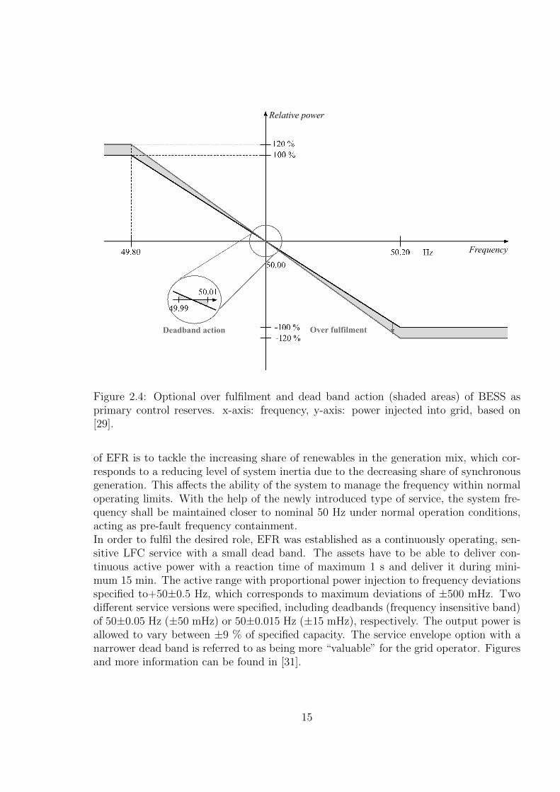
Further regulatory issues with special focus on battery storage systems as primarycontrol reserve are published in [29]. The two main aspects described below are alsoillustrated in figure 2.4:

• Deadband (frequency insensitive band). Within a deadband of ±10 mHz aroundthe set point frequency, operators of BESS are allowed to charge or discharge thebatteries for reasons of optimal battery charge management. This is optional, butrestricted to charge/discharge actions “in the right direction”, such that they sup-port the system frequency stabilisation.

• Optional over fulfilment. During primary control action, the battery storage mayprovide up to 20 % higher positive or negative power injection (in grid supportingdirection) in order to support the battery charge management.

Enhanced Frequency Response In the interconnected transmission grid of GreatBritain, the system operator National Grid Electricity Transmission (NGET) launcheda first tender round for a new type of load frequency control service in 2016, [30]. Theso-called “Enhanced Frequency Response” (EFR) was introduced in addition to existingprimary and secondary response services, which in this grid are requested to full deliverwithin 10 s/30 s, and be sustained for 30 s/30 min, respectively. The main objective

14

Relative power

Frequency

Over fulfilmentDeadband action

100 %120 %

50.00

50.2049.80

50.01

49.99

Hz

-100 %-120 %

Figure 2.4: Optional over fulfilment and dead band action (shaded areas) of BESS asprimary control reserves. x-axis: frequency, y-axis: power injected into grid, based on[29].

of EFR is to tackle the increasing share of renewables in the generation mix, which cor-responds to a reducing level of system inertia due to the decreasing share of synchronousgeneration. This affects the ability of the system to manage the frequency within normaloperating limits. With the help of the newly introduced type of service, the system fre-quency shall be maintained closer to nominal 50 Hz under normal operation conditions,acting as pre-fault frequency containment.In order to fulfil the desired role, EFR was established as a continuously operating, sen-sitive LFC service with a small dead band. The assets have to be able to deliver con-tinuous active power with a reaction time of maximum 1 s and deliver it during mini-mum 15 min. The active range with proportional power injection to frequency deviationsspecified to+50±0.5 Hz, which corresponds to maximum deviations of ±500 mHz. Twodifferent service versions were specified, including deadbands (frequency insensitive band)of 50±0.05 Hz (±50 mHz) or 50±0.015 Hz (±15 mHz), respectively. The output power isallowed to vary between ±9 % of specified capacity. The service envelope option with anarrower dead band is referred to as being more “valuable” for the grid operator. Figuresand more information can be found in [31].

15

2.3.4 Dynamic load frequency response model

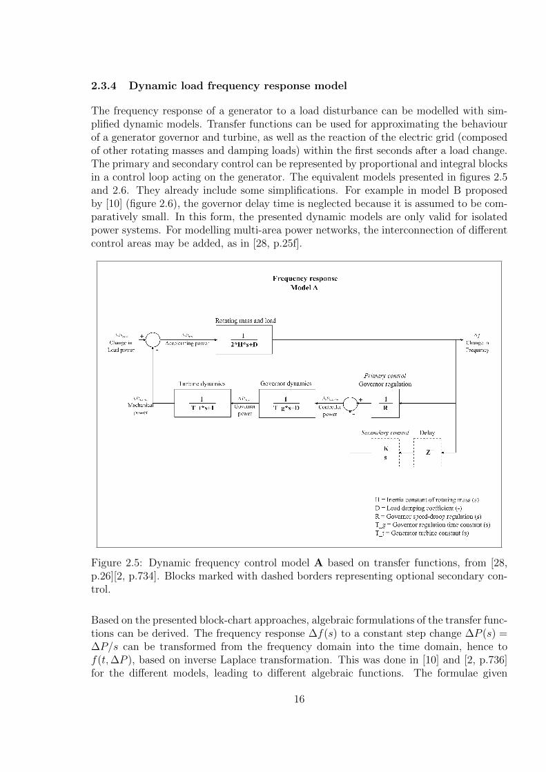
The frequency response of a generator to a load disturbance can be modelled with sim-plified dynamic models. Transfer functions can be used for approximating the behaviourof a generator governor and turbine, as well as the reaction of the electric grid (composedof other rotating masses and damping loads) within the first seconds after a load change.The primary and secondary control can be represented by proportional and integral blocksin a control loop acting on the generator. The equivalent models presented in figures 2.5and 2.6. They already include some simplifications. For example in model B proposedby [10] (figure 2.6), the governor delay time is neglected because it is assumed to be com-paratively small. In this form, the presented dynamic models are only valid for isolatedpower systems. For modelling multi-area power networks, the interconnection of differentcontrol areas may be added, as in [28, p.25f].

Figure 2.5: Dynamic frequency control model A based on transfer functions, from [28,p.26][2, p.734]. Blocks marked with dashed borders representing optional secondary con-trol.

Based on the presented block-chart approaches, algebraic formulations of the transfer func-tions can be derived. The frequency response ∆f(s) to a constant step change ∆P (s) =∆P/s can be transformed from the frequency domain into the time domain, hence tof(t,∆P ), based on inverse Laplace transformation. This was done in [10] and [2, p.736]for the different models, leading to different algebraic functions. The formulae given

16

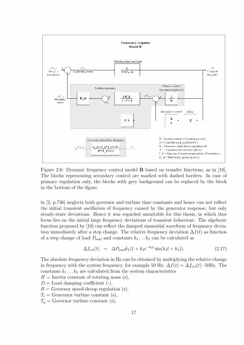
Figure 2.6: Dynamic frequency control model B based on transfer functions, as in [10].The blocks representing secondary control are marked with dashed borders. In case ofprimary regulation only, the blocks with grey background can be replaced by the blockin the bottom of the figure.

in [2, p.736] neglects both governor and turbine time constants and hence can not reflectthe initial transient oscillation of frequency caused by the generator response, but onlysteady-state deviations. Hence it was regarded unsuitable for this thesis, in which theefocus lies on the initial large frequency deviations of transient behaviour. The algebraicfunction proposed by [10] can reflect the damped sinusoidal waveform of frequency devia-tion immediately after a step change. The relative frequency deviation ∆f(t) as functionof a step change of load Pload and constants k1 . . . k5 can be calculated as

∆frel(t) = ∆Ploadk1(1 + k2e−k3t sin(k4t+ k5)). (2.17)

The absolute frequency deviation in Hz can be obtained by multiplying the relative changein frequency with the system frequency, for example 50 Hz: ∆f(t) = ∆frel(t) · 50Hz. Theconstants k1 . . . k5 are calculated from the system characteristicsH = Inertia constant of rotating mass (s),D = Load damping coefficient (-),R = Governor speed-droop regulation (s),Tt = Generator turbine constant (s),Tg = Governor turbine constant (s),

17

Fh = Fraction of power generated by high pressure (HP) turbine (-),Km = Mechanical power gain (-),R = Governor speed-droop regulation (-)with

k1 =R

DR +Km

k2 = α

√1− 2Ttk21k22 + Tt

2k212

1− k222

k3 = k21k22

k4 = k21

√1− k22

2

k5 = arctan

(k4Tt

1− k21k22Tt

)− arctan

(k4Tt

1− k21k22Tt

)k21 =

√DR +Km

2HRTt

k22 = k21

(2HR + Tt(DR +KmFh)

2(DR +Km)

).

The factor α was added manually for enhancing the fitting of the algebraic function tothe underlying dynamic model B from the same publication [10], and also with regard tomodel A from [28] and [2]. The effect of model parameters on dynamic frequency responsecharacteristics is as follows.

• The delay times of the turbine and governor Tt and Tg influence the strength ofexponential damping on initial sinusoidal oscillation. Longer delay times result ina more damped, and also reduced maximum frequency deviation and shorter timeuntil the steady-state deviation is reached, [10].

• Also the HP turbine fraction Fh has an influence on damping. The higher thisvalue, the more damped the frequency response, [10].

• The system inertia constant H influences the initial slope, time and value ofmaximum frequency deviation. The higher the value of system inertia, the later themaximum deviation is reached, which is smaller too. Equivalent inertia values oflarge power systems vary over time, and are expected to decrease in future due toa higher share of RES in the grid, [27].

• The factor D represents the damping effect of loads, which is a change in demandpower at different frequencies. It proportionally influences the frequency deviationcaused by a load change. The frequency deviation is reduced by a higher dampingfactor value, [10].

• As expected, the primary regulation factor R has among the highest influence onthe maximum value of frequency deviation. A higher value of R leads to a reducedmaximum deviation occurring earlier in time, [10].

18

• The secondary control factor K determines how fast the steady-state frequencydeviation will be reduced to zero. It is only relevant when the secondary control is in-cluded in the model. Being delayed by several seconds to minutes, secondary controlusually does not influence the initial dynamic behaviour of frequency change, [28][2].

2.4 Li-ion based battery energy storage

The amount of electrical Energy Storages Systems (ESS) for different grid connectedapplications has been increasing significantly during the last decades. Initially being de-ployed in isolated grids, Battery Energy Storage Systems (BESS) are increasingly usedfor providing a wide range of grid-supporting services.The need of storage solutions in the electricity grid results from both variability of demandon the consumer side, and, increasingly, of fluctuating and difficult to predict renewableenergy sources on the generation side, [32]. Thus particularly in countries aiming at atransition from conventional energy sources to RES, electric storages are beginning toplay a larger role in different types of services, as the decreasing amount of conventionalthermal power plant results in less capacity that is able to provide frequency regulationservices, [33]. Furthermore, the characteristic dynamic behaviour of systems with regardto a lower and more variable system inertia value is changed, [27]. Possible applications ofBESS include energy time-shift, black-start capability and reserve power for generators,frequency regulation and other power quality services such as voltage support and en-hanced integration of RES. The basic operation of a BESS in all types of services can besummarised as energy charging or discharging of different forms over a certain period oftime. It results in absorption or injection of active or reactive power, [32]. Lithium-Ion (Li-ion) based BESS are particularly suitable for short-term frequency regulation services dueto small response times and high cycle efficiencies compared to other types of electricalstorages, [34]. Batteries of this type are also characterised by relatively small dimensionsand weights, which is however of minor importance for fixed applications. High costshave been considered the main drawback of battery storage systems in the past, but arecontinuously decreasing.Electrochemical storages are characterised by certain charge and discharge characteristics,caused by the underlying chemical reactions and operating conditions, such as ambienttemperature. Electrochemical or electronic equivalent circuit models can represent suchcharacteristics. Model parameters can be obtained with experiments. For example, [35]proposes a dynamic battery model, based on different mathematical descriptions duringcharge and discharge actions. An equivalent electric circuit model is given in [26]. ForLi-ion based batteries, the extend of dynamic phenomena such as variance of voltage atdifferent charge/discharge currents and SOC, is comparatively low. Hence, large Li-ionbased BESS can be modelled as a flexible current source with a constant voltage levelin less detailed simulation studies. Dependencies of the charge/discharge voltage on theinstantaneous current and SOC are neglected within a certain range of operation. Thenominal voltage of a BESS is defined by the number of connected single battery cells. Theoutput voltage may be adjusted by the converter unit that couples the DC-based batterywith a commonly AC-based grid. Additionally to voltage and current, also the operating

19

temperature of large-scale storages is assumed to be maintainable in a small range withthe help of cooling systems. Naturally, all these assumptions should be validated whenoperating a real battery storage.

20

3 Model based predictive control

In this chapter, the control strategy used for the battery storage will be presented. Sec-tion 3.1 summarises the working principle of model predictive control and section 3.2introduces a possible optimisation method for the objective function.

3.1 Model predictive control

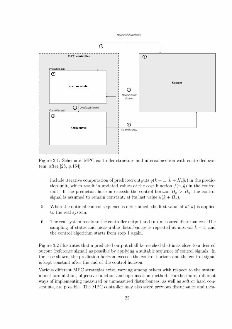
Model Predictive Control (MPC) is an effective control strategy for linear and nonlinearsystems in the presence of uncertainties, disturbances and constraints, [36]. As illus-trated by the schematic structure in figure 3.1, the MPC controller consists of two maincomponents,

• a prediction unit containing a model of the system, possibly also further aspectssuch as disturbance modelling,

• and a control unit, which is basically the optimisation unit.

The prediction unit’s function is to forecast the future behaviour of the controlled systemwhen a specific controller output sequence, a control signal entering the real system, wouldbe applied. The purpose of the controller unit is, in turn, to determine the optimal controlsignal, among all possible sequences as specified by physical or other constraints. Thedesirability of any control signal is usually assessed by means of an objective function(cost function) that shall be minimised. During the optimisation process, the expectedperformance of different possible controller outputs is evaluated by the controller unit, [28,p.153f].

3.1.1 Working principle

The numbers in figure 3.1 indicate the following sequence of controller actions, [28, p.154].In continuous operation, they are conducted repeatedly. The process is also illustrated infigure 3.2, including the different horizons.

1. At a sampling interval k, state(s) and/or output measurements x(k), y(k) of the realsystem are obtained and transferred to the controller.

2. Based on real system measurements and an initial sequence of control signals overthe control horizon Hu, u(k...k + Hu|k), from the control unit, the prediction unitsimulates the system behaviour over the prediction horizon Hp. Particularly in thepresence of constraints, the initial control signal is required to be feasible.

3. The predicted output y(k + 1...k +Hp|k) is transferred to the controller.

4. The optimal control sequence u∗(k + 1...k + Hu|k) is determined by the controlunit, based on the specified optimisation method. The optimisation process may

21

Objectives

Controller unit

MPC controller

System

Measured disturbance

Predicted Output

Control signal

Measurement

of states

Prediction unit

1

3

1

4

5

6

Figure 3.1: Schematic MPC controller structure and interconnection with controlled sys-tem, after [28, p.154].

include iterative computation of predicted outputs ˆy(k + 1...k +Hp|k) in the predic-tion unit, which result in updated values of the cost function f(u, y) in the controlunit. If the prediction horizon exceeds the control horizon Hp > Hu, the controlsignal is assumed to remain constant, at its last value u(k +Hu).

5. When the optimal control sequence is determined, the first value of u∗(k) is appliedto the real system.

6. The real system reacts to the controller output and (un)measured disturbances. Thesampling of states and measurable disturbances is repeated at interval k + 1, andthe control algorithm starts from step 1 again.

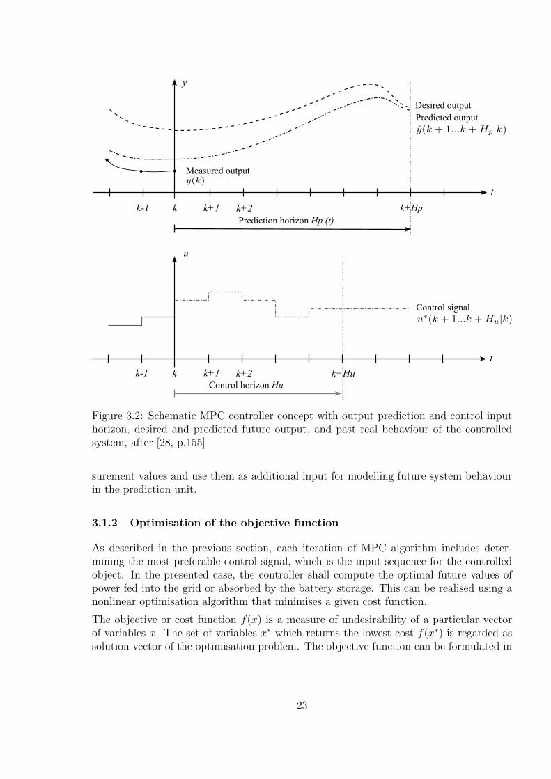
Figure 3.2 illustrates that a predicted output shall be reached that is as close to a desiredoutput (reference signal) as possible by applying a suitable sequence of control signals. Inthe case shown, the prediction horizon exceeds the control horizon and the control signalis kept constant after the end of the control horizon.

Various different MPC strategies exist, varying among others with respect to the systemmodel formulation, objective function and optimisation method. Furthermore, differentways of implementing measured or unmeasured disturbances, as well as soft or hard con-straints, are possible. The MPC controller may also store previous disturbance and mea-

22

t

t

k

u

k+1 k+2 k+Huk-1

Control signal

Control horizon Hu

k

y

k+1 k+2 k+Hpk-1

Desired output

Predicted output

Measured output

Prediction horizon Hp (t)

Figure 3.2: Schematic MPC controller concept with output prediction and control inputhorizon, desired and predicted future output, and past real behaviour of the controlledsystem, after [28, p.155]

surement values and use them as additional input for modelling future system behaviourin the prediction unit.

3.1.2 Optimisation of the objective function

As described in the previous section, each iteration of MPC algorithm includes deter-mining the most preferable control signal, which is the input sequence for the controlledobject. In the presented case, the controller shall compute the optimal future values ofpower fed into the grid or absorbed by the battery storage. This can be realised using anonlinear optimisation algorithm that minimises a given cost function.

The objective or cost function f(x) is a measure of undesirability of a particular vectorof variables x. The set of variables x∗ which returns the lowest cost f(x∗) is regarded assolution vector of the optimisation problem. The objective function can be formulated in

23

different ways, for example as summed k weighted optimisation criteria fi(x), i = 1, ..., k

f(x) =k∑i=1

wifi(x), (3.1)

with weigths w ∈ <k, or as weighted norms of optimisation criteria, for example absolutevalues

f(x) =k∑i=1

wi|fi(x)|. (3.2)

Other expressions and norms such as quadratic terms or maxima (infinite norm), andcombinations are possible. The cost function for a specific optimisation problem is for-mulated with regard to applicable objectives and their importance, taking into accountthe selected optimisation algorithm and convergence properties.

The purpose of a minimisation algorithm is to solve an unconstrained optimisation prob-lem. This can be applied to the minimisation of an objective function f(x) : <n 7→ <,

minimise f(x), (3.3)

with regard to the arguments (optimisation variables) x = (x1, ..., xn), [37, p.1]. Thiscorresponds to finding the optimal vector x∗, for which the objective function f has itssmallest value among all possible vectors x: for any x, f(x) ≥ f(x∗). The optimizationproblem is called linear, if the objective function f is linear, otherwise it is nonlinear.

3.2 Nelder-Mead simplex optimisation

The numeric Nelder-Mead simplex method was applied in the form of a Matlab function,fminsearch. The principle for multidimensional unconstrained minimization was firstpublished in [38] and described in [39]. It is also known as downhill simplex method.As direct search method, the algorithm has the advantage of being derivative-free andeasy to implement on the one hand. On the other hand, it is basically heuristic and notguaranteed to converge to a local or even global minimum, [40][39]. The following sectionswill further explain the optimisation method.

3.2.1 Nelder-Mead simplex algorithm

In Nelder-Mead algorithm, the optimisation of n variables, which corresponds to findingthe minimum of the objective function in an n-dimensional space <n, is performed by usingan n-dimensional simplex. This simplex is a type of polyhedra formed by n+ 1 differentpoints (vertices). For example in 1-dimensional space the simplex will be a line definedby two points; a two-dimensional simplex is a triangle, including its interior; and a 3-dimensional simplex would be a tetrahedron with 4 vertices [37]. During the minimisationprocess, an initial simplex is moving and adapting itself to the local landscape (of theobjective function), and finally contracts onto a minimum [39].

24

In each iteration, based on the calculated values of the objective function f(xi) at severalsurrounding points xi, the NelderMead simplex can change in the five different ways:Reflection, Expansion, Outside contraction, Inside contraction or Shrink.In all cases but shrinking, the vertex with the “worst” (highest) value of the objectivefunctionis replaced by a new point in <n, [40], moving the simplex in the direction ofthe smallest calculated cost function value. The downhill simplex method is a directsearch method, which means it does not require analytical or numerical determination ofderivatives. It is only necessary to determine a number of specific values of the objectivefunction f in each iteration, at least one for each vertex. This may be computationallyexpensive, but makes the algorithm suitable for computer-based minimisation of complexnonlinear real-world problems, [40]. However, depending on the surface of the objectivefunction, problems of false and premature convergence of downhill simplex algorithm havebeen reported by several sources, as in [41].

3.2.2 Optimisation with inequality constraints

The Nelder-Mead simplex was originally proposed for minimisation of unconstrained ob-jective functions, [40]. However, real-world problems usually contain some form of physicalconstraints, e.g. the operating range of generators or other machines. It is possible to ex-pand the optimisation method by including m equality or inequality constraints, set by theconstraint functions ci : <n 7−→ <, i = 1...m with constant limits (bounds) b1, ..., bm, [37,p.1], leading to

minimise f(x) (3.4)

subject to ci(x) ≤ bi, i = 1...m. (3.5)

The solution vector x∗ shall be determined as the vector that has the smallest objectivevalue among all vectors that satisfy the given constraints.Constrained optimisation problems can be approximated with unconstrained methodscombined with penalty functions, [42]. In accordance with such penalty functions,additional terms are added to the cost function if any constraints are violated. Thispenalty term implies a significant increase in costs, which makes the algorithm unlikelyto converge beyond the constraint boundaries. Using penalty functions enables an opti-misation process only inside the feasible region, hence finding a feasible initial startingpoint is essential for applying this strategy. In [43], it is proposed to extend the Matlab-function fminsearch based Nelder-Mead optimisation by inequality constraints usinginfinite barriers as penalty functions.

Barrier function terms may be included in the cost function in order to implicitlyrepresent constraints. Using such terms, feasible points are favoured that are further awayfrom the specified boundaries compared to those which are closer to the constraints. Thevalue of a barrier function increases if the vector of optimisation variables x approachesthe specific boundary, becoming very high (infinite) at the constraint value, similar topenalty functions. However, barrier functions are only applied inside the feasible region.The most common barrier function is the logarithmic function

Φi(x) = 1t

log(−ci(x)), (3.6)

25

for any of the m constraint functions ci(x), i = 1, ...,m with the parameter t, [37, p.562f].The function goes towards infinity for values close to zero. As t increases, so does the slopeof the barrier function Φi(x) close to the boundary, which for this function is zero. Thiscorresponds to an increasing accuracy of approximation to the indicator function I−(u)which is zero for all positive values of u and zero, and infinite for all values below zero:

I−(u) =

{0 for u ≥ 0

∞ for u < 0

}

3.3 Golden section search optimisation

When evaluating the performance of the controller, as described in chapter 5, it wasobserved that the first element of the optimised control signal has the largest influenceon the controller behaviour. Furthermore, the determined sequences did not always showthe desired positive effect on the system in continuous operation. Thus, it was consideredto apply a more simple and faster optimisation algorithm.It was decided to use golden the section search method. The derivative-free algorithm veryefficient for determining extrema of an objective functions in one dimension, [44]. It aimsat solving an unconstrained minimisation problem within a specified interval [xlow, xup],which is assumed to contain one single minimum. This is related to monotonic increaseand decrease of the objective function herein, [45]. In each iteration, the objective functionvalues of two points inside the interval are computed. The points are determined basedon their distance to the lower and upper bounds

(Φ− 1)(xup − xlow) =

√5− 1

2(xup − xlow) ≈ 0.6180(xup − xlow),

applying the “golden ratio” Φ =√

5+12≈ 1.6180. Out of the two points

x1 = xlow + (Φ− 1)(xup − xlow)and

x2 = xup − (Φ− 1)(xup − xlow),

the one with the lower cost function value is selected for replacing one of the intervalbounds (the bound it is closer to) in the next iteration’s interval. The algorithm isstopped at a small difference between the calculated two points’ cost function values orwhen a very small interval size is reached.

26

4 Modelling and control algorithm

This chapter will present the detailed structure and working principle of the proposedcontroller. After introducing the basic steps performed by the control algorithm in 4.1,the modelling approaches of the single components are presented in 4.2. Section 4.3contains a summary of the selection and analysis of demand data used in the simulationcase studies. The terms of the applied objective function are introduced in 4.4.

4.1 Controller structure and algorithm

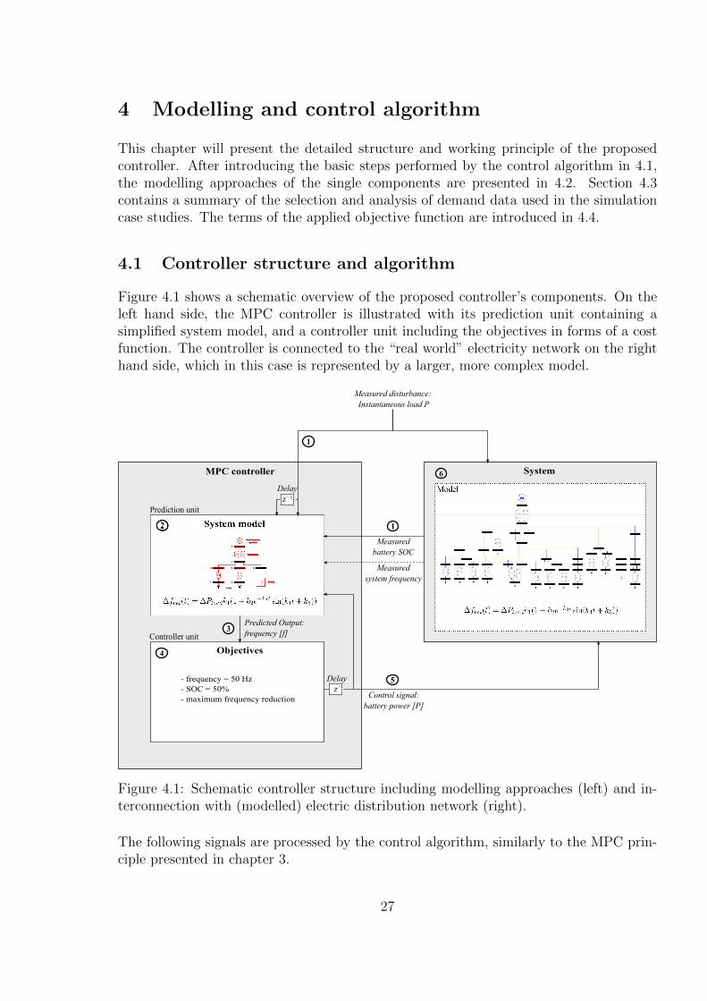
Figure 4.1 shows a schematic overview of the proposed controller’s components. On theleft hand side, the MPC controller is illustrated with its prediction unit containing asimplified system model, and a controller unit including the objectives in forms of a costfunction. The controller is connected to the “real world” electricity network on the righthand side, which in this case is represented by a larger, more complex model.

Delay

Objectives

- frequency = 50 Hz

- SOC = 50%

- maximum frequency reduction

Controller unit

MPC controller System

Measured disturbance:

Instantaneous load P

Predicted Output:

frequency [f]

Control signal:

battery power [P]

Measured

battery SOC

Delay

Prediction unit

z⁻

z⁻¹

Measured

system frequency

1

3

1

4

5

6

Figure 4.1: Schematic controller structure including modelling approaches (left) and in-terconnection with (modelled) electric distribution network (right).

The following signals are processed by the control algorithm, similarly to the MPC prin-ciple presented in chapter 3.

27

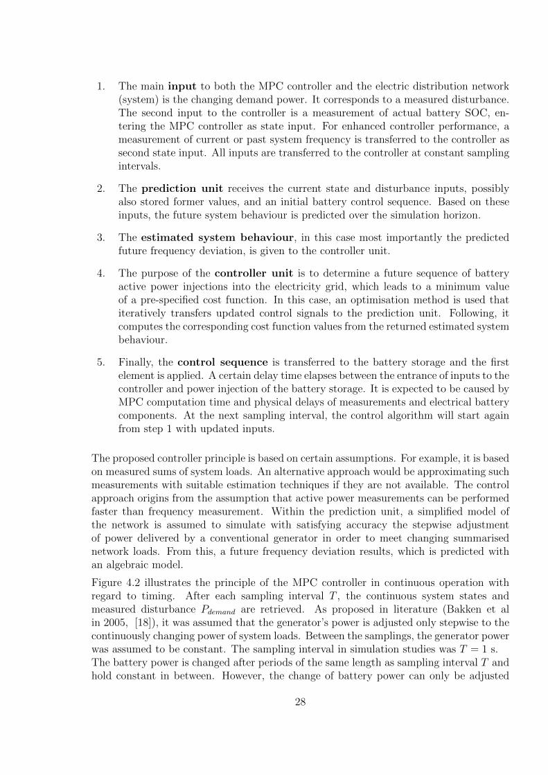
1. The main input to both the MPC controller and the electric distribution network(system) is the changing demand power. It corresponds to a measured disturbance.The second input to the controller is a measurement of actual battery SOC, en-tering the MPC controller as state input. For enhanced controller performance, ameasurement of current or past system frequency is transferred to the controller assecond state input. All inputs are transferred to the controller at constant samplingintervals.

2. The prediction unit receives the current state and disturbance inputs, possiblyalso stored former values, and an initial battery control sequence. Based on theseinputs, the future system behaviour is predicted over the simulation horizon.

3. The estimated system behaviour, in this case most importantly the predictedfuture frequency deviation, is given to the controller unit.

4. The purpose of the controller unit is to determine a future sequence of batteryactive power injections into the electricity grid, which leads to a minimum valueof a pre-specified cost function. In this case, an optimisation method is used thatiteratively transfers updated control signals to the prediction unit. Following, itcomputes the corresponding cost function values from the returned estimated systembehaviour.

5. Finally, the control sequence is transferred to the battery storage and the firstelement is applied. A certain delay time elapses between the entrance of inputs to thecontroller and power injection of the battery storage. It is expected to be caused byMPC computation time and physical delays of measurements and electrical batterycomponents. At the next sampling interval, the control algorithm will start againfrom step 1 with updated inputs.

The proposed controller principle is based on certain assumptions. For example, it is basedon measured sums of system loads. An alternative approach would be approximating suchmeasurements with suitable estimation techniques if they are not available. The controlapproach origins from the assumption that active power measurements can be performedfaster than frequency measurement. Within the prediction unit, a simplified model ofthe network is assumed to simulate with satisfying accuracy the stepwise adjustmentof power delivered by a conventional generator in order to meet changing summarisednetwork loads. From this, a future frequency deviation results, which is predicted withan algebraic model.

Figure 4.2 illustrates the principle of the MPC controller in continuous operation withregard to timing. After each sampling interval T , the continuous system states andmeasured disturbance Pdemand are retrieved. As proposed in literature (Bakken et alin 2005, [18]), it was assumed that the generator’s power is adjusted only stepwise to thecontinuously changing power of system loads. Between the samplings, the generator powerwas assumed to be constant. The sampling interval in simulation studies was T = 1 s.The battery power is changed after periods of the same length as sampling interval T andhold constant in between. However, the change of battery power can only be adjusted

28

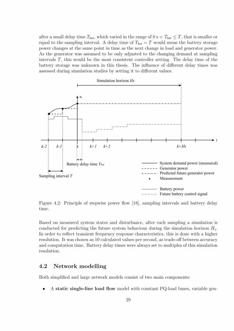
after a small delay time Tbat, which varied in the range of 0 s < Tbat ≤ T , that is smaller orequal to the sampling interval. A delay time of Tbat = T would mean the battery storagepower changes at the same point in time as the next change in load and generator power.As the generator was assumed to be only adjusted to the changing demand at samplingintervals T , this would be the most consistent controller setting. The delay time of thebattery storage was unknown in this thesis. The influence of different delay times wasassessed during simulation studies by setting it to different values.

k k+1 k+2 k+Hsk-1

Future battery control signal

Simulation horizon Hs

t

u

System demand power (measured)

k-2

Generator power

Predicted future generator power

Battery power

MeasurementSampling interval T

Battery delay time Tbat

Figure 4.2: Principle of stepwise power flow [18], sampling intervals and battery delaytime.

Based on measured system states and disturbance, after each sampling a simulation isconducted for predicting the future system behaviour during the simulation horizon Hs.In order to reflect transient frequency response characteristics, this is done with a higherresolution. It was chosen as 10 calculated values per second, as trade-off between accuracyand computation time. Battery delay times were always set to multiples of this simulationresolution.

4.2 Network modelling

Both simplified and large network models consist of two main components:

• A static single-line load flow model with constant PQ-load buses, variable gen-

29

erator slack buses, and line data representing network transmission lines and trans-formers.

• And a dynamic frequency deviation model, forecasting future values of systemfrequency caused by a step change in generator power.

The two models are presented in the following sections, followed by the modelling approachfor the battery storage.

4.2.1 Static electricity network model

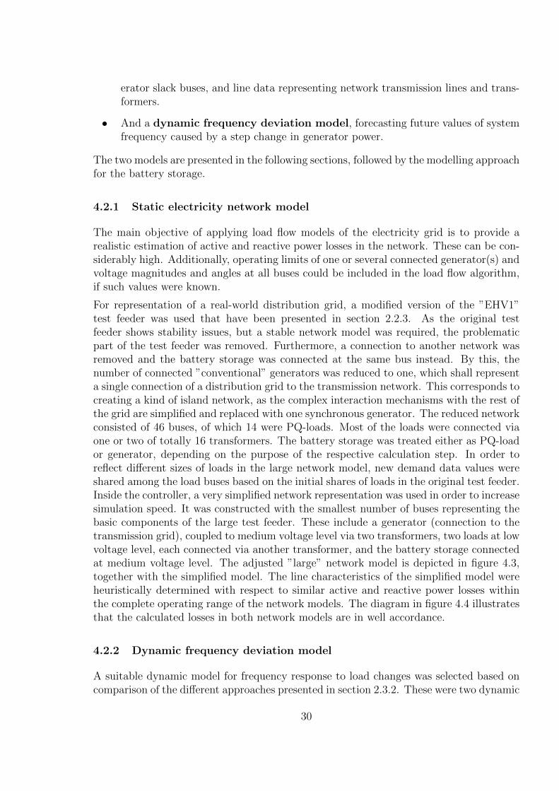
The main objective of applying load flow models of the electricity grid is to provide arealistic estimation of active and reactive power losses in the network. These can be con-siderably high. Additionally, operating limits of one or several connected generator(s) andvoltage magnitudes and angles at all buses could be included in the load flow algorithm,if such values were known.

For representation of a real-world distribution grid, a modified version of the ”EHV1”test feeder was used that have been presented in section 2.2.3. As the original testfeeder shows stability issues, but a stable network model was required, the problematicpart of the test feeder was removed. Furthermore, a connection to another network wasremoved and the battery storage was connected at the same bus instead. By this, thenumber of connected ”conventional” generators was reduced to one, which shall representa single connection of a distribution grid to the transmission network. This corresponds tocreating a kind of island network, as the complex interaction mechanisms with the rest ofthe grid are simplified and replaced with one synchronous generator. The reduced networkconsisted of 46 buses, of which 14 were PQ-loads. Most of the loads were connected viaone or two of totally 16 transformers. The battery storage was treated either as PQ-loador generator, depending on the purpose of the respective calculation step. In order toreflect different sizes of loads in the large network model, new demand data values wereshared among the load buses based on the initial shares of loads in the original test feeder.Inside the controller, a very simplified network representation was used in order to increasesimulation speed. It was constructed with the smallest number of buses representing thebasic components of the large test feeder. These include a generator (connection to thetransmission grid), coupled to medium voltage level via two transformers, two loads at lowvoltage level, each connected via another transformer, and the battery storage connectedat medium voltage level. The adjusted ”large” network model is depicted in figure 4.3,together with the simplified model. The line characteristics of the simplified model wereheuristically determined with respect to similar active and reactive power losses withinthe complete operating range of the network models. The diagram in figure 4.4 illustratesthat the calculated losses in both network models are in well accordance.

4.2.2 Dynamic frequency deviation model

A suitable dynamic model for frequency response to load changes was selected based oncomparison of the different approaches presented in section 2.3.2. These were two dynamic

30

~

-

(a) Large network model (modified UK ”EHV1” distribu-tion test feeder, [14]).

~

-

Grid connection

/ generator

Transformer

Battery

Loads

1

2

4

53

6

7

(b) Simplified networkmodel.

Figure 4.3: Comparison large and small network model.

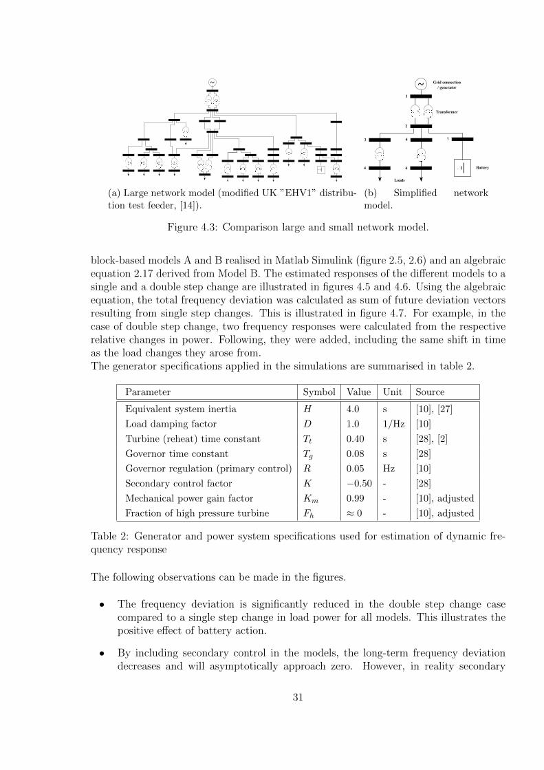
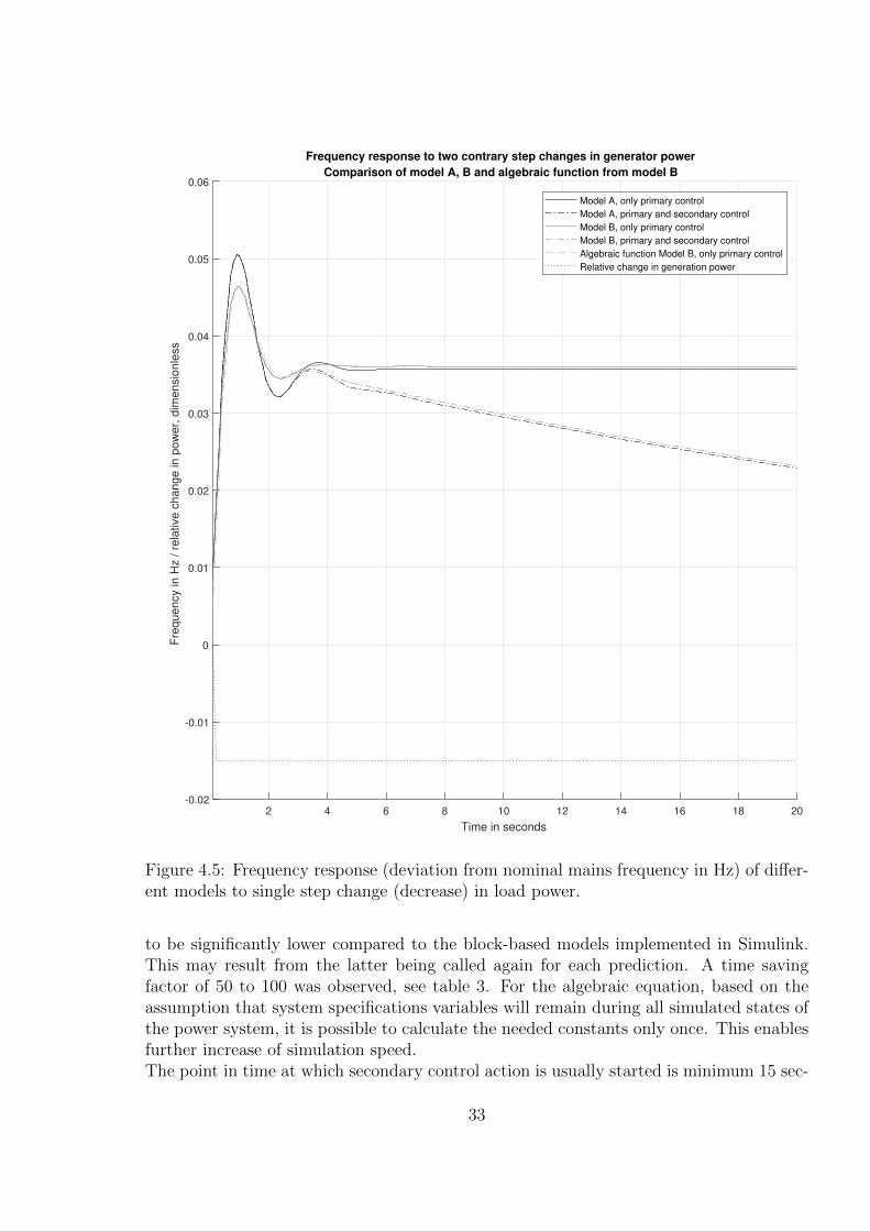
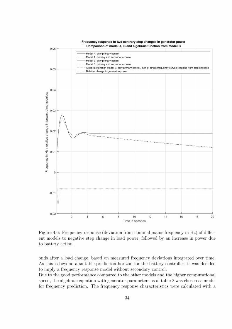
block-based models A and B realised in Matlab Simulink (figure 2.5, 2.6) and an algebraicequation 2.17 derived from Model B. The estimated responses of the different models to asingle and a double step change are illustrated in figures 4.5 and 4.6. Using the algebraicequation, the total frequency deviation was calculated as sum of future deviation vectorsresulting from single step changes. This is illustrated in figure 4.7. For example, in thecase of double step change, two frequency responses were calculated from the respectiverelative changes in power. Following, they were added, including the same shift in timeas the load changes they arose from.The generator specifications applied in the simulations are summarised in table 2.

Parameter Symbol Value Unit Source

Equivalent system inertia H 4.0 s [10], [27]

Load damping factor D 1.0 1/Hz [10]

Turbine (reheat) time constant Tt 0.40 s [28], [2]

Governor time constant Tg 0.08 s [28]

Governor regulation (primary control) R 0.05 Hz [10]

Secondary control factor K −0.50 - [28]

Mechanical power gain factor Km 0.99 - [10], adjusted

Fraction of high pressure turbine Fh ≈ 0 - [10], adjusted

Table 2: Generator and power system specifications used for estimation of dynamic fre-quency response

The following observations can be made in the figures.

• The frequency deviation is significantly reduced in the double step change casecompared to a single step change in load power for all models. This illustrates thepositive effect of battery action.

• By including secondary control in the models, the long-term frequency deviationdecreases and will asymptotically approach zero. However, in reality secondary

31

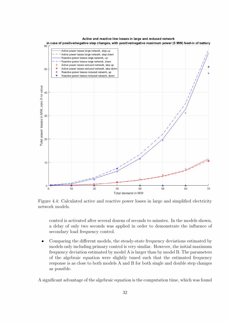
Figure 4.4: Calculated active and reactive power losses in large and simplified electricitynetwork models.

control is activated after several dozens of seconds to minutes. In the models shown,a delay of only two seconds was applied in order to demonstrate the influence ofsecondary load frequency control.

• Comparing the different models, the steady-state frequency deviations estimated bymodels only including primary control is very similar. However, the initial maximumfrequency deviation estimated by model A is larger than by model B. The parametersof the algebraic equation were slightly tuned such that the estimated frequencyresponse is as close to both models A and B for both single and double step changesas possible.

A significant advantage of the algebraic equation is the computation time, which was found

32

2 4 6 8 10 12 14 16 18 20

Time in seconds

-0.02

-0.01

0

0.01

0.02

0.03

0.04

0.05

0.06F

requency in H

z / r

ela

tive c

hange in p

ow

er,

dim

ensio

nle

ss

Frequency response to two contrary step changes in generator power

Comparison of model A, B and algebraic function from model B

Model A, only primary control

Model A, primary and secondary control

Model B, only primary control

Model B, primary and secondary control

Algebraic function Model B, only primary control

Relative change in generation power

Figure 4.5: Frequency response (deviation from nominal mains frequency in Hz) of differ-ent models to single step change (decrease) in load power.

to be significantly lower compared to the block-based models implemented in Simulink.This may result from the latter being called again for each prediction. A time savingfactor of 50 to 100 was observed, see table 3. For the algebraic equation, based on theassumption that system specifications variables will remain during all simulated states ofthe power system, it is possible to calculate the needed constants only once. This enablesfurther increase of simulation speed.The point in time at which secondary control action is usually started is minimum 15 sec-

33

2 4 6 8 10 12 14 16 18 20

Time in seconds

-0.02

-0.01

0

0.01

0.02

0.03

0.04

0.05

0.06F

requency in H

z / r

ela

tive c

hange in p

ow

er,

dim

ensio

nle

ss

Frequency response to two contrary step changes in generator power

Comparison of model A, B and algebraic function from model B

Model A, only primary control

Model A, primary and secondary control

Model B, only primary control

Model B, primary and secondary control

Algebraic function Model B, only primary control, sum of single frequency curves resulting from step changes

Relative change in generation power

Figure 4.6: Frequency response (deviation from nominal mains frequency in Hz) of differ-ent models to negative step change in load power, followed by an increase in power dueto battery action.

onds after a load change, based on measured frequency deviations integrated over time.As this is beyond a suitable prediction horizon for the battery controller, it was decidedto imply a frequency response model without secondary control.Due to the good performance compared to the other models and the higher computationalspeed, the algebraic equation with generator parameters as of table 2 was chosen as modelfor frequency prediction. The frequency response characteristics were calculated with a

34

resolution of 0.1 s, which corresponds to 10 values per second and was assumed to reflectexpected changes in frequency properly. Only primary, but not secondary control actionwas included in the model, which is acceptable as discussed above.

Desired effect of battery storage

Each recorded variation of system loads causes, in the simulations stepwise, change in thegenerator active power. This results in a frequency deviation characteristic that can beestimated with the selected model.The intended role of the battery storage connected to the electric network was to actas an additional, flexible and controllable load. By suitable battery action, thus changeof actual active power injected into the grid, generator changes should be triggered thatcause frequency deviations in the opposite direction to the former dynamic frequencyresponse. This principle is illustrated in figure 4.7. The first dynamic frequency responseis changed by a change in generator power in order to meet a variable demand. Following,the battery power is changed. By this, a new value of total system loads is achieved thathave to be delivered by the generator. This second change in generator power will leadto another frequency deviation, which preferable should be in opposite direction to theinitial one, such that the total deviation (sum of single dynamic responses) is minimised.The battery storage action that causes another change in generator power is delayed bysome small time period. Hence, the amount of battery power needed to minimise thetotal frequency deviation was expected to be slightly different from the initial systemload change. Additionally, the battery storage is the connection to the electric grid ata single point, in contrast to the distributed system loads. Thus any battery action wasexpected to result in changing line losses, that would have to be compensated by thegenerator as well and could be taken into account with suitable network models.

Applying suitable battery power vectors can lead to the following two main possibleeffects.

• a reduction of maximum predicted frequency deviation, and

• a delayed time of occurrence of maximum frequency deviation.

The first effect is the main objective of the battery storage. The second effect is small,but still considered to be positive because it ”buffers” the frequency deviation resultingfrom a change in load, meaning it offers the possibility to other load frequency controlreserves with a longer reaction time to become active.

4.2.3 Battery storage model

In section 2.4, the approximate representation of a large Li-ion based BESS as an idealcurrent source at constant output voltage was introduced. For the battery model in thisthesis, this assumption was further expanded: the storage was regarded as an ideal powersource that could deliver any required active (or reactive) power at the nominal grid

35

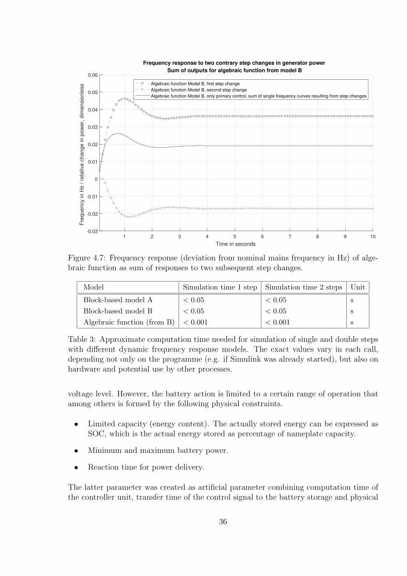
1 2 3 4 5 6 7 8 9 10

Time in seconds

-0.03

-0.02

-0.01

0

0.01

0.02

0.03

0.04

0.05

0.06

Fre

quency in H

z / r

ela

tive c

hange in p

ow

er,

dim

ensio

nle

ss

Frequency response to two contrary step changes in generator power

Sum of outputs for algebraic function from model B

Algebraic function Model B, first step change

Algebraic function Model B, second step change

Algebraic function Model B, only primary control, sum of single frequency curves resulting from step changes

Figure 4.7: Frequency response (deviation from nominal mains frequency in Hz) of alge-braic function as sum of responses to two subsequent step changes.

Model Simulation time 1 step Simulation time 2 steps Unit

Block-based model A < 0.05 < 0.05 s

Block-based model B < 0.05 < 0.05 s

Algebraic function (from B) < 0.001 < 0.001 s

Table 3: Approximate computation time needed for simulation of single and double stepswith different dynamic frequency response models. The exact values vary in each call,depending not only on the programme (e.g. if Simulink was already started), but also onhardware and potential use by other processes.

voltage level. However, the battery action is limited to a certain range of operation thatamong others is formed by the following physical constraints.

• Limited capacity (energy content). The actually stored energy can be expressed asSOC, which is the actual energy stored as percentage of nameplate capacity.

• Minimum and maximum battery power.

• Reaction time for power delivery.

The latter parameter was created as artificial parameter combining computation time ofthe controller unit, transfer time of the control signal to the battery storage and physical

36

delay time until power delivery at grid connection point.As minimum and maximum SOC,10% and 90% were chosen. These values correspond to the typical range of constant outputvoltage of Li-ion batteries. Furthermore any possible deep discharge effects and systemstresses are prevented, which increases the lifetime of the storage. For flexible operation ofthe battery storage, a medium state of charge should be maintained, from which batteryaction in both positive and negative power range are possible.Injecting energy into the grid at maximum power is possible, but should be avoidedduring longer periods of time. On the one hand, it may cause thermal stress on electriccomponents, and on the other hand, it will effect the battery SOC.

Regarding combinations of battery maximum power/nameplate capacity, feasible valueswere retrieved from a data sheet of the real market product ”Y.Cube 500/1.5” of “Youni-cos” Inc., [46]. As the storage product is scalable by combining single units, different bat-tery storage sizes were simulated as multiples of one storage unit, with the specificationsas in table 4. The storage is assumed to be suitable for the proposed application, as thesame manufacturer had installed a large battery plant based on Li-ion technology (lithium-manganese-oxide) that provides frequency regulation services, [33]. The 5 MW/5 MWhbattery power plant of 2013/14, which was expanded to totally 15 MW/15 MWh in 2016,is operated by WEMAG AG. It is located close to Schwerin, Germany, hence in a regionhighly penetrated with renewable energy sources, mainly wind power and can be seen asa reference case for the future application of the proposed controller. A reactions time ofthis storage systems of 200 ms was reported in [47].

Parameter Value Unit

Maximum power ±500 kVA

Nameplate capacity (energy) 887 kWh

Minimum state of charge (SOC) 10 %

Maximum state of charge (SOC) 90 %

Table 4: Battery model specifications, from Y.Cube 500/1.5, [46].

4.3 Demand data

A set of synthetic data of one year active and reactive demand power with a resolutionof 1 second was retrieved from [48] for evaluating the performance of the battery controller.The data set had been generated from two sets of real residential measurements and hencewas assumed to be representative for domestic loads in distribution networks and scalableto electric system of desired sizes. The three phase power consumption measurementswere summed for applying them in the single phase load flow algorithm. Furthermore,after analysing the relationship of active and reactive power (see section 4.3.1), only activepower values were used and reactive power was estimated proportionally.

37

4.3.1 Analysis of single phases and relationship of reactive to active power

In single line load flow calculation, all phases are assumed to be equally loaded and thuscan be replaced by one phase. This assumption was validated for the given demand dataset by means of a visual analysis. Figure 4.8 illustrates the phase-wise and total activeand reactive power over one day. It can be concluded from the plots that

• Active power is approximately equally distributed among the three phases. Peakloads in single do occur seldom and randomly. Hence, the single phase active powervalues can be represented by their sum.

• A daily pattern is visible for active power consumption, with times of high load inthe morning and evening hours, and low consumption during the night.

• Reactive power in different phases varies more than active power. The sum ofreactive power consumption is mostly significantly lower than for active power (indiagram: pay attention to different scales). There is no clear continuous dailydemand profile as for active power, only a phase of low reactive power consumptionduring night time.

• Active power consumption is purely positive, which indicates absence of any gener-ating sources, such as distributed PV installations. Those would result in negativeloads when more energy would be generated than consumed. Thus, the flow ofenergy within the grid is mono directional from the generator to the load(s).

• Reactive power consumption is mainly positive, which represents inductive loads(such as motors), but can be partly negative, indicating capacitive consumers.

Reactive and active power

For simplified controller design and implementation, it was examined if instantaneous re-active power values could be estimated in a simple manner from active powers. A visualanalysis of the demand data set, shown in figure 4.9, revealed that the ratio of reactiveto active power ratio Q/P is approximately normally distributed around a mean valueof Q/P = 0.11 (see lower subplot), though with a relatively large standard deviationof σ(Q/P ) = 0.051. A correlation analysis resulted in a relatively low correlation coeffi-cient (as measure of linear dependence between two variables) between active and reactivepower of ρ(P,Q) = 0.77, which is in accordance with the large variance value. The valuesof Q/P , σ(Q/P ) and ρ(P,Q) were calculated with the complete data set of one year.

The middle subplot of 4.9 does not indicate any clear dependency between Q/P ratioand the time of the day. Though, this was further evaluated with a scatter plot, seefigure 4.10. In the plot, different typical Q/P values during certain periods of the day canbe observed. However, a correlation coefficient of ρ(Q/P, t) = 0.24 indicates that there isno simple linear relationship between the two variables.It was decided to approximate the Q/P ratio as a constant proportion of 0.10 in the

38

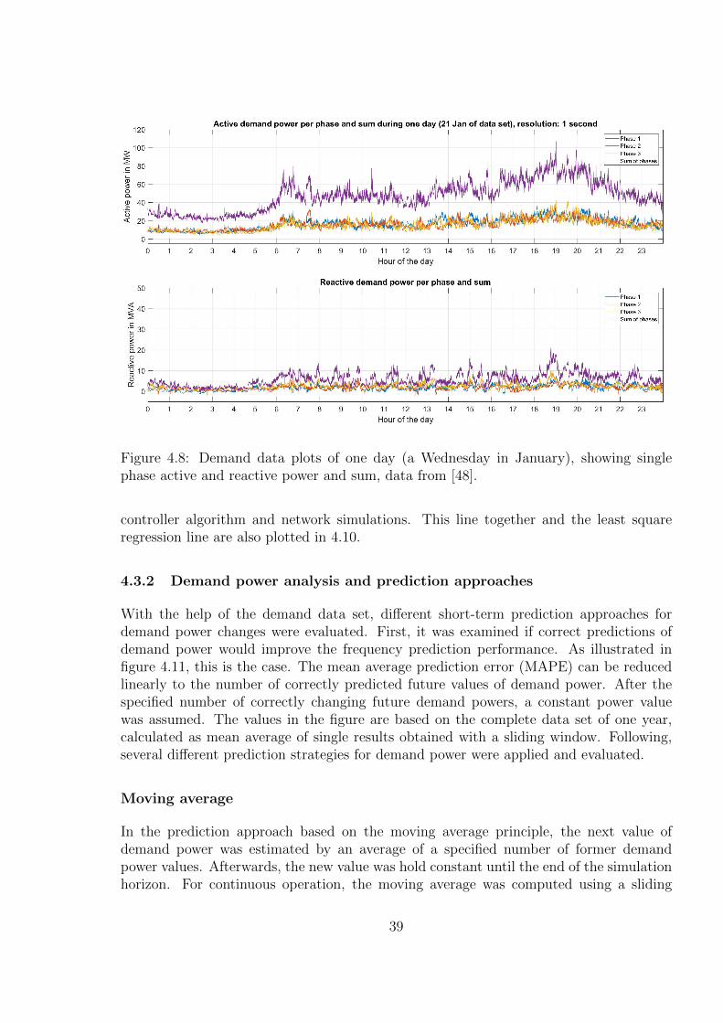
Figure 4.8: Demand data plots of one day (a Wednesday in January), showing singlephase active and reactive power and sum, data from [48].

controller algorithm and network simulations. This line together and the least squareregression line are also plotted in 4.10.

4.3.2 Demand power analysis and prediction approaches

With the help of the demand data set, different short-term prediction approaches fordemand power changes were evaluated. First, it was examined if correct predictions ofdemand power would improve the frequency prediction performance. As illustrated infigure 4.11, this is the case. The mean average prediction error (MAPE) can be reducedlinearly to the number of correctly predicted future values of demand power. After thespecified number of correctly changing future demand powers, a constant power valuewas assumed. The values in the figure are based on the complete data set of one year,calculated as mean average of single results obtained with a sliding window. Following,several different prediction strategies for demand power were applied and evaluated.

Moving average

In the prediction approach based on the moving average principle, the next value ofdemand power was estimated by an average of a specified number of former demandpower values. Afterwards, the new value was hold constant until the end of the simulationhorizon. For continuous operation, the moving average was computed using a sliding

39

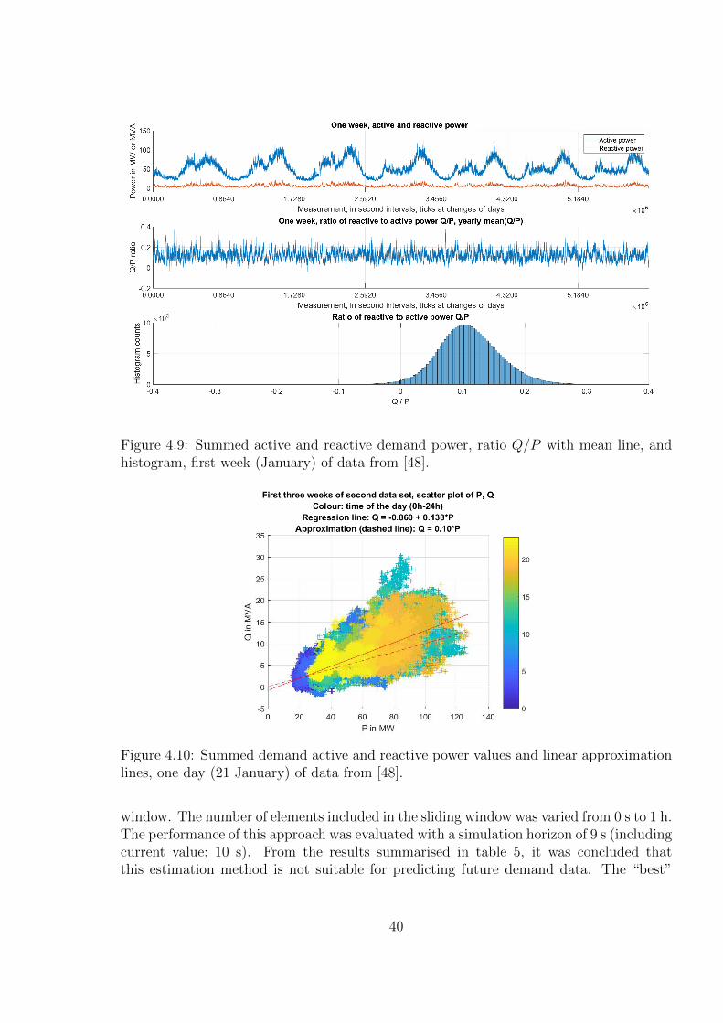
Figure 4.9: Summed active and reactive demand power, ratio Q/P with mean line, andhistogram, first week (January) of data from [48].

Figure 4.10: Summed demand active and reactive power values and linear approximationlines, one day (21 January) of data from [48].

window. The number of elements included in the sliding window was varied from 0 s to 1 h.The performance of this approach was evaluated with a simulation horizon of 9 s (includingcurrent value: 10 s). From the results summarised in table 5, it was concluded thatthis estimation method is not suitable for predicting future demand data. The “best”

40

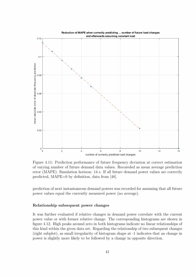
Figure 4.11: Prediction performance of future frequency deviation at correct estimationof varying number of future demand data values. Recoreded as mean average predictionerror (MAPE). Simulation horizon: 14 s. If all future demand power values are correctlypredicted, MAPE=0 by definition, data from [48].

prediction of next instantaneous demand powers was recorded for assuming that all futurepower values equal the currently measured power (no average).

Relationship subsequent power changes

It was further evaluated if relative changes in demand power correlate with the currentpower value or with former relative change. The corresponding histograms are shown infigure 4.12. High peaks around zero in both histograms indicate no linear relationships ofthis kind within the given data set. Regarding the relationship of two subsequent changes(right subplot), as small irregularity of histogram shape at -1 indicates that an change inpower is slightly more likely to be followed by a change in opposite direction.

41

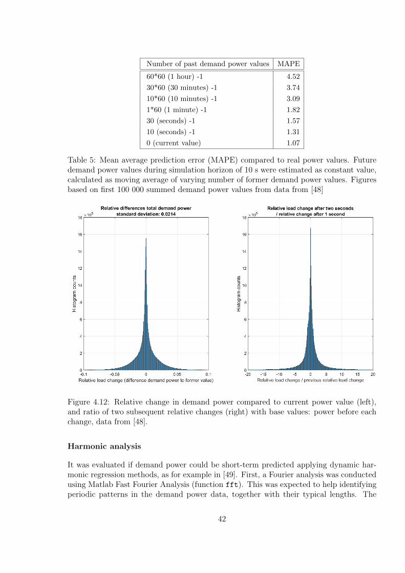
Number of past demand power values MAPE

60*60 (1 hour) -1 4.52

30*60 (30 minutes) -1 3.74

10*60 (10 minutes) -1 3.09

1*60 (1 minute) -1 1.82

30 (seconds) -1 1.57

10 (seconds) -1 1.31

0 (current value) 1.07

Table 5: Mean average prediction error (MAPE) compared to real power values. Futuredemand power values during simulation horizon of 10 s were estimated as constant value,calculated as moving average of varying number of former demand power values. Figuresbased on first 100 000 summed demand power values from data from [48]

Figure 4.12: Relative change in demand power compared to current power value (left),and ratio of two subsequent relative changes (right) with base values: power before eachchange, data from [48].

Harmonic analysis

It was evaluated if demand power could be short-term predicted applying dynamic har-monic regression methods, as for example in [49]. First, a Fourier analysis was conductedusing Matlab Fast Fourier Analysis (function fft). This was expected to help identifyingperiodic patterns in the demand power data, together with their typical lengths. The

42

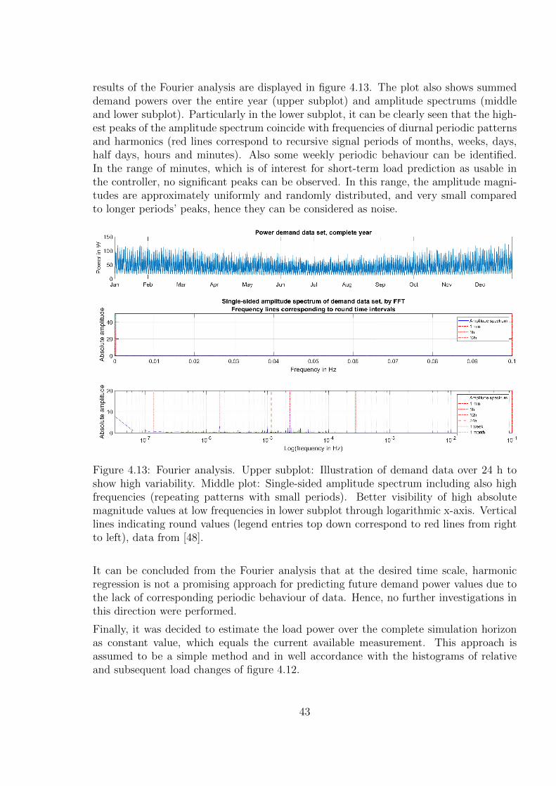
results of the Fourier analysis are displayed in figure 4.13. The plot also shows summeddemand powers over the entire year (upper subplot) and amplitude spectrums (middleand lower subplot). Particularly in the lower subplot, it can be clearly seen that the high-est peaks of the amplitude spectrum coincide with frequencies of diurnal periodic patternsand harmonics (red lines correspond to recursive signal periods of months, weeks, days,half days, hours and minutes). Also some weekly periodic behaviour can be identified.In the range of minutes, which is of interest for short-term load prediction as usable inthe controller, no significant peaks can be observed. In this range, the amplitude magni-tudes are approximately uniformly and randomly distributed, and very small comparedto longer periods’ peaks, hence they can be considered as noise.

Figure 4.13: Fourier analysis. Upper subplot: Illustration of demand data over 24 h toshow high variability. Middle plot: Single-sided amplitude spectrum including also highfrequencies (repeating patterns with small periods). Better visibility of high absolutemagnitude values at low frequencies in lower subplot through logarithmic x-axis. Verticallines indicating round values (legend entries top down correspond to red lines from rightto left), data from [48].

It can be concluded from the Fourier analysis that at the desired time scale, harmonicregression is not a promising approach for predicting future demand power values due tothe lack of corresponding periodic behaviour of data. Hence, no further investigations inthis direction were performed.

Finally, it was decided to estimate the load power over the complete simulation horizonas constant value, which equals the current available measurement. This approach isassumed to be a simple method and in well accordance with the histograms of relativeand subsequent load changes of figure 4.12.

43

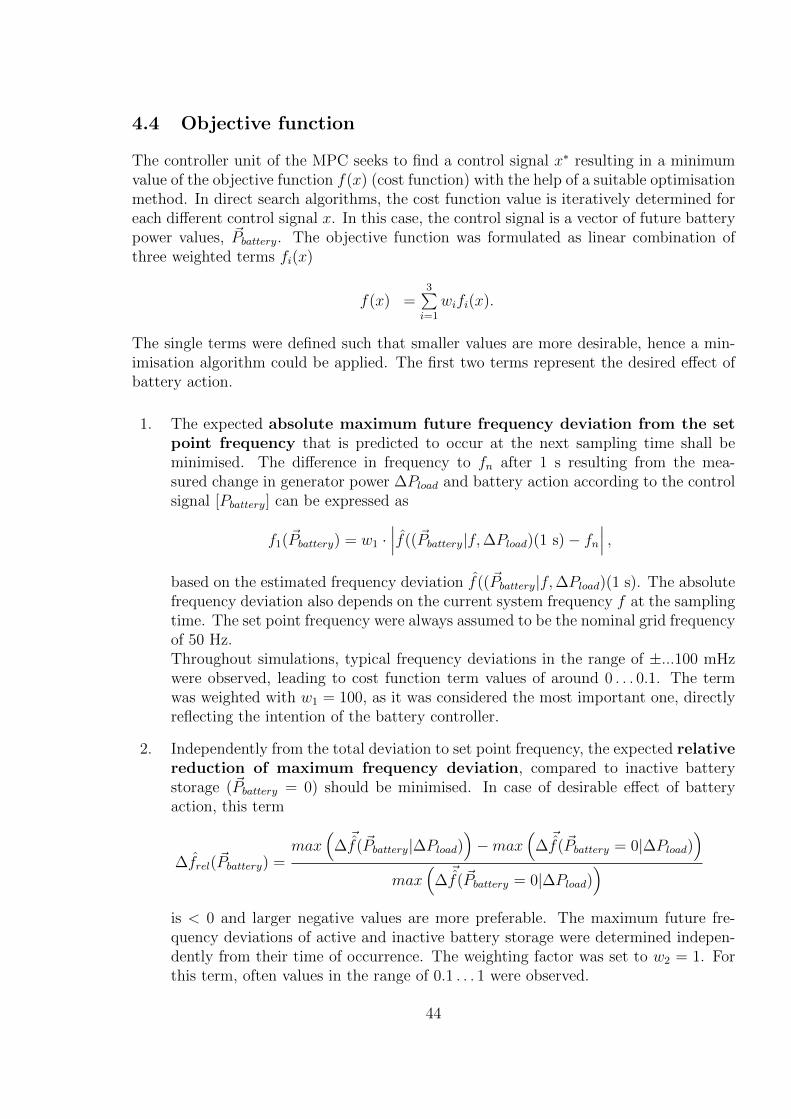
4.4 Objective function

The controller unit of the MPC seeks to find a control signal x∗ resulting in a minimumvalue of the objective function f(x) (cost function) with the help of a suitable optimisationmethod. In direct search algorithms, the cost function value is iteratively determined foreach different control signal x. In this case, the control signal is a vector of future batterypower values, ~Pbattery. The objective function was formulated as linear combination ofthree weighted terms fi(x)

f(x) =3∑i=1

wifi(x).

The single terms were defined such that smaller values are more desirable, hence a min-imisation algorithm could be applied. The first two terms represent the desired effect ofbattery action.

1. The expected absolute maximum future frequency deviation from the setpoint frequency that is predicted to occur at the next sampling time shall beminimised. The difference in frequency to fn after 1 s resulting from the mea-sured change in generator power ∆Pload and battery action according to the controlsignal [Pbattery] can be expressed as

f1(~Pbattery) = w1 ·∣∣∣f((~Pbattery|f,∆Pload)(1 s)− fn

∣∣∣ ,based on the estimated frequency deviation f((~Pbattery|f,∆Pload)(1 s). The absolutefrequency deviation also depends on the current system frequency f at the samplingtime. The set point frequency were always assumed to be the nominal grid frequencyof 50 Hz.Throughout simulations, typical frequency deviations in the range of ±...100 mHzwere observed, leading to cost function term values of around 0 . . . 0.1. The termwas weighted with w1 = 100, as it was considered the most important one, directlyreflecting the intention of the battery controller.

2. Independently from the total deviation to set point frequency, the expected relativereduction of maximum frequency deviation, compared to inactive batterystorage (~Pbattery = 0) should be minimised. In case of desirable effect of batteryaction, this term

∆frel(~Pbattery) =max

(∆~f(~Pbattery|∆Pload)

)−max

(∆~f(~Pbattery = 0|∆Pload)

)max

(∆~f(~Pbattery = 0|∆Pload)

)is < 0 and larger negative values are more preferable. The maximum future fre-quency deviations of active and inactive battery storage were determined indepen-dently from their time of occurrence. The weighting factor was set to w2 = 1. Forthis term, often values in the range of 0.1 . . . 1 were observed.

44

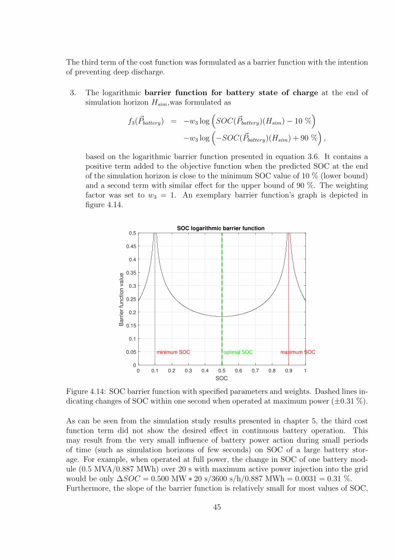
The third term of the cost function was formulated as a barrier function with the intentionof preventing deep discharge.

3. The logarithmic barrier function for battery state of charge at the end ofsimulation horizon Hsim,was formulated as

f3(~Pbattery) = −w3 log(SOC(~Pbattery)(Hsim)− 10 %

)−w3 log

(−SOC(~Pbattery)(Hsim) + 90 %

),

based on the logarithmic barrier function presented in equation 3.6. It contains apositive term added to the objective function when the predicted SOC at the endof the simulation horizon is close to the minimum SOC value of 10 % (lower bound)and a second term with similar effect for the upper bound of 90 %. The weightingfactor was set to w3 = 1. An exemplary barrier function’s graph is depicted infigure 4.14.

0 0.1 0.2 0.3 0.4 0.5 0.6 0.7 0.8 0.9 1

SOC

0

0.05

0.1

0.15

0.2

0.25

0.3

0.35

0.4

0.45

0.5

Ba

rrie

r fu

nctio

n v

alu

e

SOC logarithmic barrier function

minimum SOC maximum SOCoptimal SOC

Figure 4.14: SOC barrier function with specified parameters and weights. Dashed lines in-dicating changes of SOC within one second when operated at maximum power (±0.31 %).

As can be seen from the simulation study results presented in chapter 5, the third costfunction term did not show the desired effect in continuous battery operation. Thismay result from the very small influence of battery power action during small periodsof time (such as simulation horizons of few seconds) on SOC of a large battery stor-age. For example, when operated at full power, the change in SOC of one battery mod-ule (0.5 MVA/0.887 MWh) over 20 s with maximum active power injection into the gridwould be only ∆SOC = 0.500 MW ∗ 20 s/3600 s/h/0.887 MWh = 0.0031 = 0.31 %.Furthermore, the slope of the barrier function is relatively small for most values of SOC,

45

except extreme values, leading to small influence on the cost function.As an alternative approach, it could be considered to limit the SOC to the operatingrange with a penalty function. In order to prevent constant charge or discharge action, asuitable additional barrier function could be applied that penalises constant operation ofbattery at high power in one direction over long periods of time.

Any hard constraints on the optimisation problem were realised as infinite penalty func-tion terms added to the objective function in case of specified barriers being exceeded.However, in this application, all physical constraints were included directly in the calcula-tion of battery power vectors, in order to ensure they would be never exceeded. By doingso, the possible problem of infeasible starting points in the optimisation algorithm wasavoided, which can arise when imposing constraints directly on the optimisation method.

46

5 Simulation studies

This chapter presents a simulation study, which was conducted with the aim of evaluatingthe controller performance in continuous operation and for comparing different operatingmodes, controller and battery designs. A vector of demand power from the same periodof time was used in all different variants. All simulations were conducted with bothoptimisation algorithms presented in chapter 3: Nelder-Mead simplex optimisation andgolden section search method.

5.1 Comparison of operating modes

The performance of the MPC control algorithm should be compared to other operatingmodes of the battery storage. The computed modes were inactive battery, LFC-similaroperation and the proposed MPC controller, as described below.

(I.) In inactive battery storage (“no battery”) mode, the values of active and reactivepower injected into the grid were zero at all times. Mode (I) should representsimulations of original power system’s behaviour without BESS.

(II.) In load frequency control (LFC) mode, the battery was requested to feed in activepower proportionally to the currently measured frequency deviation, in accordancewith regulations in the Continental European interconnected synchronous area (asdescribed in section 2.3.3). It was assumed that system frequency was sampledat the same point in time as the demand power values, hence at intervals of 1second. The frequency deviations caused at that moment were not yet includedin the frequency measurement, meaning it actually represents the last sampling’sfrequency. The battery power was determined proportionally to frequency deviation,up to its maximum power. Deadband action was included in the range of smalldeviations from set point system frequency. It was only activated when havingpositive effect on battery SOC, driving it closer to 50 %. Over fulfilment was notincluded in the algorithm. The calculated change of battery power was applied afterthe specified battery delay time. Afterwards, the battery power was held constantuntil the next change.

(III.) In the third operating mode, the battery storage’s reacted to measured changesin total system load, based on the model predictive control (MPC) algorithmpresented in the former chapter.

The simulation of ”real” power system only included primary control action, which is partof the frequency deviation model recursively computed after each sampling time. It was alarger, more complex version of the system model inside the MPC controller, which clearlyfocussed on short-term calculations. Not including secondary or tertiary control actionlimits the feasible time ranges for evaluation of controller performance to small periods, asload-following over longer periods (> 15 . . . 30 s) is the main task of these control services.Dismissing them, the model won’t be able to represent slow adaption of the power system

47

to a new load-generation power equilibrium. Furthermore, in real interconnected powergrids, also interchange of energy with other control areas helps stabilising the system. Theused algorithm did not contain these processes. Hence, results of simulations over shortperiods of time were expected to be more realistic and reliable compared to simulatinglonger periods of time.

5.2 Load data

For evaluating the performance of the proposed control algorithm in continuous operation,it should be applied during in a simulation of a representative period of time. After eachsampling, a battery control signal would be computed by MPC controller and returned tothe ”real” system model, in which the system behaviour including battery storage actionis simulated. The computed system frequency and battery SOC would be then used ascontroller input at the next sampling instance, together with the next value of the demandpower vector.

It was considered to simulate periods of weeks or days from different seasons of the year inorder to evaluate different load patterns and magnitudes. However, due to the algorithmlimitations to short periods of time, it was not feasible to compute whole days or evenweeks. Thus, and also due to low computational speed, it was decided to select periods ofmaximum half an hour. The selected period of time was during morning hours (6 h-7 h)with intervals of mainly rising, but also and falling demand power values. The selectedtime of 20 min is illustrated in figure 5.1.

When used for simulations, the selected vector of power values were scaled such thatit was in the middle of the used load flow simulation network’s feasible range (also seefigure 4.4 in section 4.2). The original load power of the test feeder was 38 MW ac-tive power, and maximum applicable total power the modified network was found to bearound 60 MW to 70 MW, with any exceedance leading to non convergence of the loadflow algorithm.

5.3 Parameter variation

In simulation studies, different system and controller parameters were varied in order toevaluate the proposed LFC control algorithm and compare it to the other operationalmodes presented in section 5.1. The same sequence of demand data, selected according tosection 5.2, was used in all simulations. Each simulation run consisted of an initialisation,in which system states were reset to their nominal values, a simulation phase, in whichall time values of the demand vector were simulated and the battery storage reactedaccording to the respective operating mode. The system states and outputs of interestwere stored for each time step. After fully simulating one variant case, some pre-specifiedperformance criteria were determined from the stored values. The following differentbattery parameters were varied.

• Battery size by means of nominal capacity/maximum power. This parameter wasvaried with the aim of evaluating the influence of battery size on the controller’s

48

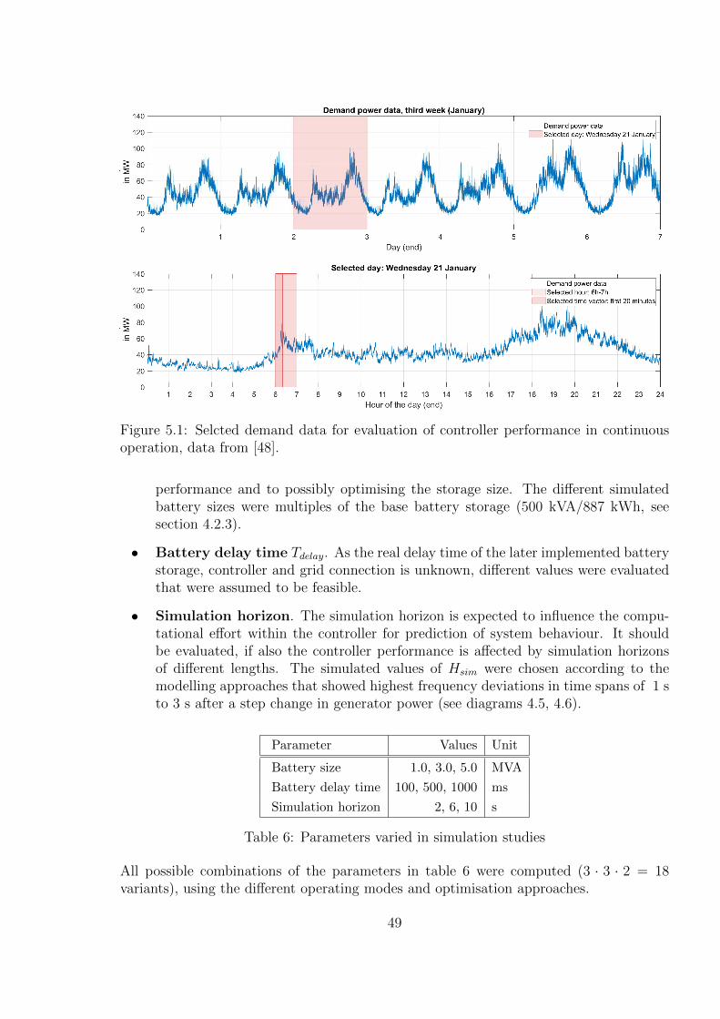
Figure 5.1: Selcted demand data for evaluation of controller performance in continuousoperation, data from [48].

performance and to possibly optimising the storage size. The different simulatedbattery sizes were multiples of the base battery storage (500 kVA/887 kWh, seesection 4.2.3).

• Battery delay time Tdelay. As the real delay time of the later implemented batterystorage, controller and grid connection is unknown, different values were evaluatedthat were assumed to be feasible.

• Simulation horizon. The simulation horizon is expected to influence the compu-tational effort within the controller for prediction of system behaviour. It shouldbe evaluated, if also the controller performance is affected by simulation horizonsof different lengths. The simulated values of Hsim were chosen according to themodelling approaches that showed highest frequency deviations in time spans of 1 sto 3 s after a step change in generator power (see diagrams 4.5, 4.6).

Parameter Values Unit

Battery size 1.0, 3.0, 5.0 MVA

Battery delay time 100, 500, 1000 ms

Simulation horizon 2, 6, 10 s

Table 6: Parameters varied in simulation studies

All possible combinations of the parameters in table 6 were computed (3 · 3 · 2 = 18variants), using the different operating modes and optimisation approaches.

49

5.4 Performance evaluation

In order to compare the controller performance in the different variants, in each simulationthe following variables were recorded:

• Vector of battery power Pbat.

• Vector of battery SOC.

• Vector of system frequency fsys.

• Vector of expected relative reduction of predicted maximum frequency deviation.

• Vector of expected relative reduction of area under predicted frequency deviationover the simulation horizon.

• Total time needed for simulation of the variant in each mode.

These result values were used to compute some performance measures for each simu-lated variant, operating mode, and optimisation method:

• Mean average of system frequency f sys. The closer this value is to the nominalgrid frequency, the better the average performance of the controller.

• Standard deviation of system frequency σ(fsys), representing the variabilityof system frequency. As large frequency deviations are undesirable, a value close tozero is preferable.

• State of charge at the end of the simulation period. The final SOC after a certainperiod of operation is an indirect measure of overall energy injected into or absorbedfrom the grid. If total sum of positive and negative powers are equal, this variablewould be zero. Being calculated relative to the storage capacity, SOC values areindependent from the battery size and hence suitable for comparison of differentdesign cases.

• Variability of battery power, by means of the sum of absolute differences inpower injected into or absorbed from the grid by the battery storage. Many largechanges in power will lead to a higher value. Because this figure correlates with thebattery size (larger battery designs allow larger maximum power values), it is scaledby the nominal power of the storage. A small value of variability is preferable, as itis assumed that many, especially large changes in power injection stress all electricalcomponents and thus lead to earlier ageing effects and higher costs of maintenanceand replacement.

5.5 Results and analysis

This section presents the simulation study results, analysis and interpretation. It includesthe comparison of the two proposed optimisation algorithms. All referenced result plotscan be found in section 5.5.6.

50

5.5.1 System frequency without battery action

The diagrams in section 5.5.6, for example figure 5.2, illustrate the values of several systemparameters of interest computed in continuous simulation over 20 min. The subplots onthe left hand side present results of the operating mode II (load frequency control) and theright ones of operating mode III (MPC). In both plots, the calculated system frequency isplotted in blue, and the system frequency modelled without battery storage (mode I) inlight blue. The demand power data, as selected in the previous section, is plotted in grey.A moving average line in black illustrates the overall increase of demand power duringthe simulated period.In operating mode I (inactive battery storage), two main observations can be made withregard to the observed system frequency, see for example figure 5.2.

• The system frequency tends to decrease over time due to the increasing summedsystem loads. In real power systems, secondary control services would be activatedto compensate the long long-term distortions of active power balance.

• The frequency deviations computed with the current settings of frequency responsecharacteristic model are comparatively large. It is assumed that a realistic parametri-sation would lead to much smaller variations in the power system frequency.

5.5.2 Observed issues with different operating modes and optimisation algo-rithms

The calculated battery power is indicated with a red line in the plots. In all computedvariants, the same undesirable behaviour of the battery storage after a certain time canbe observed: the battery system “hangs”, meaning it keeps almost constantly feedingin energy at maximum power. Through this, the energy stored in the battery is reducedwithout having any positive effect on the frequency of the connected power system.In case of operating mode II (LFC), the effect is assumed to result from large measuredfrequency deviations, to which the battery reacts with proportional power, as requestedby the regulations. Measured large system frequency deviations are partly caused by thechanging demand power and the very sensitive frequency response model, as discussedabove. However, also the extreme reaction of the battery storage itself can cause largefrequency deviations, sometimes leading to short periods of oscillation. The effect is morelikely to occur at larger battery sizes, as the requested battery power is proportional tothe storage size. At small battery sizes and fast reaction (small battery delay times), thedesired stabilising effect of the battery storage on the system frequency can be observed,for example in figure 5.2, at least in the initial period of the demand vector. The systemfrequency throughout the remaining simulated time depends on the frequency value atthe time when the undesirable battery behaviour begins.In operating mode III (MPC), the effect of hanging battery storage was observed too,particularly at small battery storage sizes and long delay times. The reasons for hangingare suspected to lay mostly with the used optimisation methods and the form of the costfunction.

51

It can be observed that the compensation of frequency deviations by the battery storageis similar to load following. However, long periods of frequency directions in one directioncan cause problems to both optimisation algorithms, in a similar way to storages ofdifferent size, as illustrated in figures 5.3 and 5.5. When working constantly at maximumpower, the controller’s task would be to detect the instances when a deviating batterypower would have a positive effect due to the changed state of the power system. Thisexpected behaviour could not be observer for either of the two optimisation algorithms.The golden section search method resulted in almost constant maximum power injections,see figures 5.2 and 5.3. The MPC with Nelder-Mead simplex optimisation returned evenbattery control signals that lead to larger system frequency deviations compared to aninctive battery storage, as it is visible in figures 5.4 and 5.5. Some further issues related tothe used Nelder-Mead simplex algorithm were detected when analysing the optimisationprocess. For example, often initial changes of the simplex in an undesirable direction wereobserved, but they could not be influenced in an efficient way. Furthermore, unsuitableinitial step sizes of simplex changes were detected, leading to ignorance of more suitablebattery power values. The initial step size could not be directly controlled either in thechosen algorithm. Hence the golden section optimisation algorithm should be preferred.

5.5.3 Varying battery storage size

The effect of battery storage size on the controller performance have been partly describedin the previous section. When comparing the system frequency with an MPC-battery tothe system frequency in operating mode I (no battery action), it can be concluded thatlarge battery storages can lead to a good stabilisation of frequency. In figures 5.2, 5.3, 5.4and 5.5 it can be seen that the plotted graphs of larger batteries are closer to the set pointfrequency of 50 Hz, at least as long as the battery storage acts in the intended way. Withregard to operating mode II (LFC), smaller storages show more desirable performance.This is related to frequency deviations caused by large storage power values, as discussedabove.

The effect of different battery storage sizes on the frequency stabilisation performance issummarised in figure 5.6 for the golden section search and in figure 5.7 for the Nelder-Mead simplex optimisation. The influence of other varied parameters is discussed inthe following sections. The diagrams show that the average system frequency deviatesmore from the set point frequency when applying the proposed methods, than withoutbattery storage. In operating mode II (middle subplot), the performance clearly decreaseswith increasing battery size. Only for large battery storages with Nelder-Mead simplexoptimisation (figure 5.7, right subplot), a small reduction of mean frequency deviationcan be observed.

As further performance measurement, the standard deviation of the computed system fre-quency vector was computed. It can be seen in figure 5.8 that the system frequency can bestabilised when applying an MPC with golden section search methods, with improving per-formance at larger battery sizes. The performance of the simplex optimisation-based MPCvaries (figure 5.9). The implemented LFC algorithm did not show any stabilising effect.

52

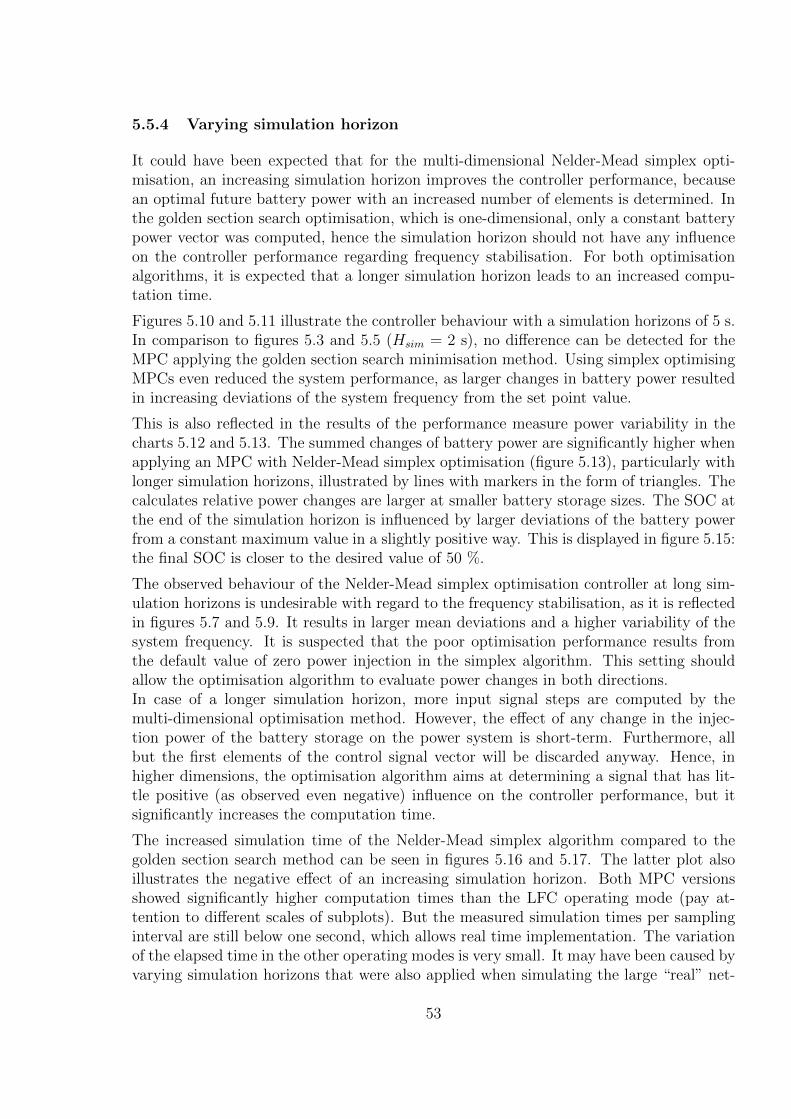
5.5.4 Varying simulation horizon

It could have been expected that for the multi-dimensional Nelder-Mead simplex opti-misation, an increasing simulation horizon improves the controller performance, becausean optimal future battery power with an increased number of elements is determined. Inthe golden section search optimisation, which is one-dimensional, only a constant batterypower vector was computed, hence the simulation horizon should not have any influenceon the controller performance regarding frequency stabilisation. For both optimisationalgorithms, it is expected that a longer simulation horizon leads to an increased compu-tation time.

Figures 5.10 and 5.11 illustrate the controller behaviour with a simulation horizons of 5 s.In comparison to figures 5.3 and 5.5 (Hsim = 2 s), no difference can be detected for theMPC applying the golden section search minimisation method. Using simplex optimisingMPCs even reduced the system performance, as larger changes in battery power resultedin increasing deviations of the system frequency from the set point value.

This is also reflected in the results of the performance measure power variability in thecharts 5.12 and 5.13. The summed changes of battery power are significantly higher whenapplying an MPC with Nelder-Mead simplex optimisation (figure 5.13), particularly withlonger simulation horizons, illustrated by lines with markers in the form of triangles. Thecalculates relative power changes are larger at smaller battery storage sizes. The SOC atthe end of the simulation horizon is influenced by larger deviations of the battery powerfrom a constant maximum value in a slightly positive way. This is displayed in figure 5.15:the final SOC is closer to the desired value of 50 %.

The observed behaviour of the Nelder-Mead simplex optimisation controller at long sim-ulation horizons is undesirable with regard to the frequency stabilisation, as it is reflectedin figures 5.7 and 5.9. It results in larger mean deviations and a higher variability of thesystem frequency. It is suspected that the poor optimisation performance results fromthe default value of zero power injection in the simplex algorithm. This setting shouldallow the optimisation algorithm to evaluate power changes in both directions.In case of a longer simulation horizon, more input signal steps are computed by themulti-dimensional optimisation method. However, the effect of any change in the injec-tion power of the battery storage on the power system is short-term. Furthermore, allbut the first elements of the control signal vector will be discarded anyway. Hence, inhigher dimensions, the optimisation algorithm aims at determining a signal that has lit-tle positive (as observed even negative) influence on the controller performance, but itsignificantly increases the computation time.

The increased simulation time of the Nelder-Mead simplex algorithm compared to thegolden section search method can be seen in figures 5.16 and 5.17. The latter plot alsoillustrates the negative effect of an increasing simulation horizon. Both MPC versionsshowed significantly higher computation times than the LFC operating mode (pay at-tention to different scales of subplots). But the measured simulation times per samplinginterval are still below one second, which allows real time implementation. The variationof the elapsed time in the other operating modes is very small. It may have been caused byvarying simulation horizons that were also applied when simulating the large “real” net-

53

work, and from varying number of calls of internal loops and if-cases. Also other softwarerunning on the simulation computer at the same time may have had some influence.

5.5.5 Varying battery delay time

As further parameter, the battery delay time that elapsed between sampling and changeof active power injected or absorbed by the battery storage was varied in the simulationstudies. In all performance plots, it can be seen that longer delay times lead to worsecontroller performance, except the standard deviation of system frequency and simplexoptimisation (figure5.9), and the computation times (figures 5.16 and 5.17). In the timeplots in figures 5.18 and 5.19, the formerly observed positive effects of battery storageswith shorter delay times are not visible any more. In MPC operation, the computedbattery power remains at its minimum or maximum value for most of the time. Asmentioned in section 4.1, a battery delay time equal to the sample time would actuallybe the most consistent controller design, but unfortunately revealed the least desirableperformance.

54

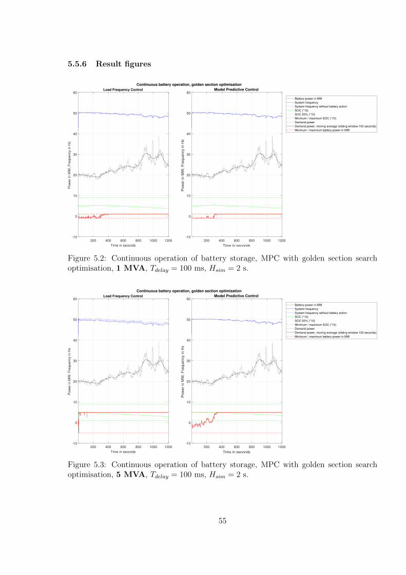
5.5.6 Result figures

200 400 600 800 1000 1200

Time in seconds

-10

0

10

20

30

40

50

60

Pow

er

in M

W, F

requency in H

z

Load Frequency Control

200 400 600 800 1000 1200

Time in seconds

-10

0

10

20

30

40

50

60

Pow

er

in M

W, F

requency in H

z

Continuous battery operation, golden section optimisation

Model Predictive Control

Battery power in MW

System frequency

System frequency without battery action

SOC (*10)

SOC 50% (*10)

Minimum / maximum SOC (*10)

Demand power

Demand power, moving average (sliding window 100 seconds)

Minimum / maximum battery power in MW

Figure 5.2: Continuous operation of battery storage, MPC with golden section searchoptimisation, 1 MVA, Tdelay = 100 ms, Hsim = 2 s.

200 400 600 800 1000 1200

Time in seconds

-10

0

10

20

30

40

50

60

Pow

er

in M

W, F

requency in H

z

Load Frequency Control

200 400 600 800 1000 1200

Time in seconds

-10

0

10

20

30

40

50

60

Pow

er

in M

W, F

requency in H

z

Continuous battery operation, golden section optimisation

Model Predictive Control

Battery power in MW

System frequency

System frequency without battery action

SOC (*10)

SOC 50% (*10)

Minimum / maximum SOC (*10)

Demand power

Demand power, moving average (sliding window 100 seconds)

Minimum / maximum battery power in MW

Figure 5.3: Continuous operation of battery storage, MPC with golden section searchoptimisation, 5 MVA, Tdelay = 100 ms, Hsim = 2 s.

55

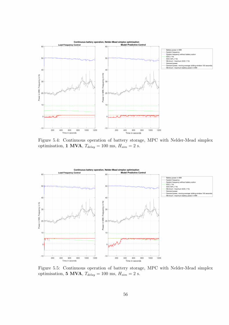
200 400 600 800 1000 1200

Time in seconds

-10

0

10

20

30

40

50

60

Pow

er

in M

W, F

requency in H

z

Load Frequency Control

200 400 600 800 1000 1200

Time in seconds

-10

0

10

20

30

40

50

60

Pow

er

in M

W, F

requency in H

z

Continuous battery operation, Nelder-Mead simplex optimisation

Model Predictive Control

Battery power in MW

System frequency

System frequency without battery action

SOC (*10)

SOC 50% (*10)

Minimum / maximum SOC (*10)

Demand power

Demand power, moving average (sliding window 100 seconds)

Minimum / maximum battery power in MW

Figure 5.4: Continuous operation of battery storage, MPC with Nelder-Mead simplexoptimisation, 1 MVA, Tdelay = 100 ms, Hsim = 2 s.

200 400 600 800 1000 1200

Time in seconds

-10

0

10

20

30

40

50

60

Pow

er

in M

W, F

requency in H

z

Load Frequency Control

200 400 600 800 1000 1200

Time in seconds

-10

0

10

20

30

40

50

60

Pow

er

in M

W, F

requency in H

z

Continuous battery operation, Nelder-Mead simplex optimisation

Model Predictive Control

Battery power in MW

System frequency

System frequency without battery action

SOC (*10)

SOC 50% (*10)

Minimum / maximum SOC (*10)

Demand power

Demand power, moving average (sliding window 100 seconds)

Minimum / maximum battery power in MW

Figure 5.5: Continuous operation of battery storage, MPC with Nelder-Mead simplexoptimisation, 5 MVA, Tdelay = 100 ms, Hsim = 2 s.

56

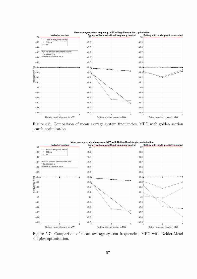
1 3 5

Battery nominal power in MW

48.5

48.6

48.7

48.8

48.9

49

49.1

49.2

49.3

49.4

49.5

49.6

49.7

49.8

49.9

50

Fre

qu

en

cy in

Hz

No battery action

Feed-in delay time 100 ms

500 ms

1 s

1 3 5

Battery nominal power in MW

48.5

48.6

48.7

48.8

48.9

49

49.1

49.2

49.3

49.4

49.5

49.6

49.7

49.8

49.9

50

Mean average system frequency, MPC with golden section optimisation

Battery with classical load frequency control

1 3 5

Battery nominal power in MW

48.5

48.6

48.7

48.8

48.9

49

49.1

49.2

49.3

49.4

49.5

49.6

49.7

49.8

49.9

50Battery with model predictive control

Markers: different simulation horizons

° 2 s, triangle 5 s

Dotted line: desirable value

Figure 5.6: Comparison of mean average system frequencies, MPC with golden sectionsearch optimisation.

1 3 5

Battery nominal power in MW

48.5

48.6

48.7

48.8

48.9

49

49.1

49.2

49.3

49.4

49.5

49.6

49.7

49.8

49.9

50

Fre

qu

en

cy in

Hz

No battery action

Feed-in delay time 100 ms

500 ms

1 s

1 3 5

Battery nominal power in MW

48.5

48.6

48.7

48.8

48.9

49

49.1

49.2

49.3

49.4

49.5

49.6

49.7

49.8

49.9

50

Mean average system frequency, MPC with Nelder-Mead simplex optimisation

Battery with classical load frequency control

1 3 5

Battery nominal power in MW

48.5

48.6

48.7

48.8

48.9

49

49.1

49.2

49.3

49.4

49.5

49.6

49.7

49.8

49.9

50Battery with model predictive control

Markers: different simulation horizons

° 2 s, triangle 5 s

Dotted line: desirable value

Figure 5.7: Comparison of mean average system frequencies, MPC with Nelder-Meadsimplex optimisation.

57

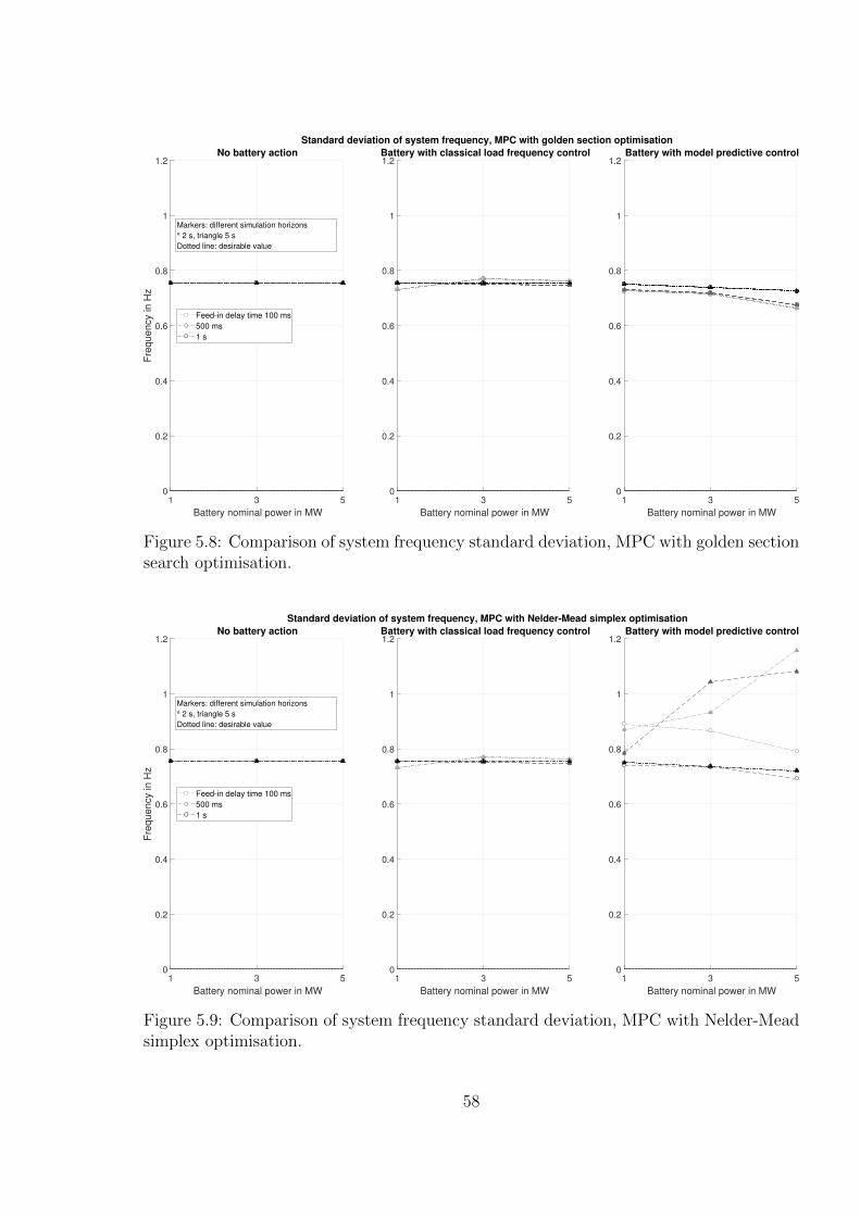
1 3 5

Battery nominal power in MW

0

0.2

0.4

0.6

0.8

1

1.2

Fre

quency in H

zNo battery action

Feed-in delay time 100 ms

500 ms

1 s

1 3 5

Battery nominal power in MW

0

0.2

0.4

0.6

0.8

1

1.2

Standard deviation of system frequency, MPC with golden section optimisation

Battery with classical load frequency control

1 3 5

Battery nominal power in MW

0

0.2

0.4

0.6

0.8

1

1.2Battery with model predictive control

Markers: different simulation horizons

° 2 s, triangle 5 s

Dotted line: desirable value

Figure 5.8: Comparison of system frequency standard deviation, MPC with golden sectionsearch optimisation.

1 3 5

Battery nominal power in MW

0

0.2

0.4

0.6

0.8

1

1.2

Fre

quency in H

z

No battery action

Feed-in delay time 100 ms

500 ms

1 s

1 3 5

Battery nominal power in MW

0

0.2

0.4

0.6

0.8

1

1.2

Standard deviation of system frequency, MPC with Nelder-Mead simplex optimisation

Battery with classical load frequency control

1 3 5

Battery nominal power in MW

0

0.2

0.4

0.6

0.8

1

1.2Battery with model predictive control

Markers: different simulation horizons

° 2 s, triangle 5 s

Dotted line: desirable value

Figure 5.9: Comparison of system frequency standard deviation, MPC with Nelder-Meadsimplex optimisation.

58

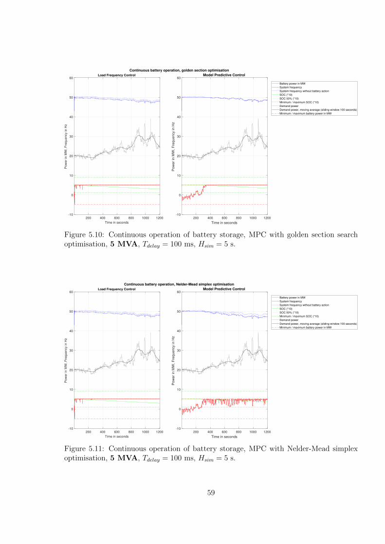
200 400 600 800 1000 1200

Time in seconds

-10

0

10

20

30

40

50

60

Pow

er

in M

W, F

requency in H

z

Load Frequency Control

200 400 600 800 1000 1200

Time in seconds

-10

0

10

20

30

40

50

60

Pow

er

in M

W, F

requency in H

z

Continuous battery operation, golden section optimisation

Model Predictive Control

Battery power in MW

System frequency

System frequency without battery action

SOC (*10)

SOC 50% (*10)

Minimum / maximum SOC (*10)

Demand power

Demand power, moving average (sliding window 100 seconds)

Minimum / maximum battery power in MW

Figure 5.10: Continuous operation of battery storage, MPC with golden section searchoptimisation, 5 MVA, Tdelay = 100 ms, Hsim = 5 s.

200 400 600 800 1000 1200

Time in seconds

-10

0

10

20

30

40

50

60

Pow

er

in M

W, F

requency in H

z

Load Frequency Control

200 400 600 800 1000 1200

Time in seconds

-10

0

10

20

30

40

50

60

Pow

er

in M

W, F

requency in H

z

Continuous battery operation, Nelder-Mead simplex optimisation

Model Predictive Control

Battery power in MW

System frequency

System frequency without battery action

SOC (*10)

SOC 50% (*10)

Minimum / maximum SOC (*10)

Demand power

Demand power, moving average (sliding window 100 seconds)

Minimum / maximum battery power in MW

Figure 5.11: Continuous operation of battery storage, MPC with Nelder-Mead simplexoptimisation, 5 MVA, Tdelay = 100 ms, Hsim = 5 s.

59

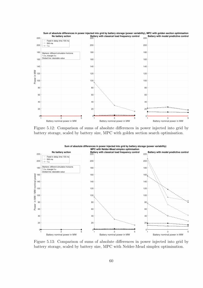
1 3 5

Battery nominal power in MW

0

20

40

60

80

100

120

140

160

180

200

220

Po

we

r in

MW

No battery action

Feed-in delay time 100 ms

500 ms

1 s

1 3 5

Battery nominal power in MW

0

20

40

60

80

100

120

140

160

180

200

220

Sum of absolute differences in power injected into grid by battery storage (power variability), MPC with golden section optimisation

Battery with classical load frequency control

1 3 5

Battery nominal power in MW

0

20

40

60

80

100

120

140

160

180

200

220

Battery with model predictive control

Markers: different simulation horizons

° 2 s, triangle 5 s

Dotted line: desirable value

Figure 5.12: Comparison of sums of absolute differences in power injected into grid bybattery storage, scaled by battery size, MPC with golden section search optimisation.

1 3 5

Battery nominal power in MW

0

20

40

60

80

100

120

140

160

180

200

220

Po

we

r in

MW

/ M

W n

om

ina

l p

ow

er

No battery action

Feed-in delay time 100 ms

500 ms

1 s

1 3 5

Battery nominal power in MW

0

20

40

60

80

100

120

140

160

180

200

220

Sum of absolute differences in power injected into grid by battery storage (power variability)

MPC with Nelder-Mead simplex optimisation

Battery with classical load frequency control

1 3 5

Battery nominal power in MW

0

20

40

60

80

100

120

140

160

180

200

220Battery with model predictive control

Markers: different simulation horizons

° 2 s, triangle 5 s

Dotted line: desirable value

Figure 5.13: Comparison of sums of absolute differences in power injected into grid bybattery storage, scaled by battery size, MPC with Nelder-Mead simplex optimisation.

60

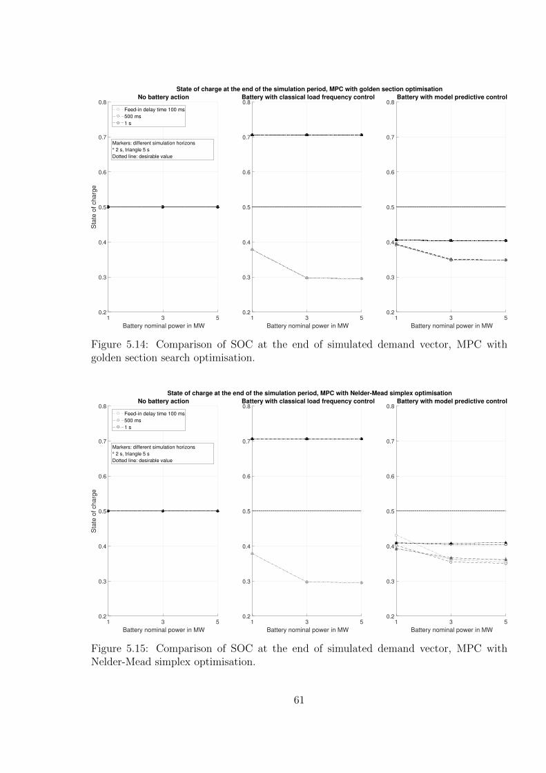
1 3 5

Battery nominal power in MW

0.2

0.3

0.4

0.5

0.6

0.7

0.8

Sta

te o

f charg

eNo battery action

Feed-in delay time 100 ms

500 ms

1 s

1 3 5

Battery nominal power in MW

0.2

0.3

0.4

0.5

0.6

0.7

0.8

State of charge at the end of the simulation period, MPC with golden section optimisation

Battery with classical load frequency control

1 3 5

Battery nominal power in MW

0.2

0.3

0.4

0.5

0.6

0.7

0.8Battery with model predictive control

Markers: different simulation horizons

° 2 s, triangle 5 s

Dotted line: desirable value

Figure 5.14: Comparison of SOC at the end of simulated demand vector, MPC withgolden section search optimisation.

1 3 5

Battery nominal power in MW

0.2

0.3

0.4

0.5

0.6

0.7

0.8

Sta

te o

f charg

e

No battery action

Feed-in delay time 100 ms

500 ms

1 s

1 3 5

Battery nominal power in MW

0.2

0.3

0.4

0.5

0.6

0.7

0.8

State of charge at the end of the simulation period, MPC with Nelder-Mead simplex optimisation

Battery with classical load frequency control

1 3 5

Battery nominal power in MW

0.2

0.3

0.4

0.5

0.6

0.7

0.8Battery with model predictive control

Markers: different simulation horizons

° 2 s, triangle 5 s

Dotted line: desirable value

Figure 5.15: Comparison of SOC at the end of simulated demand vector, MPC withNelder-Mead simplex optimisation.

61

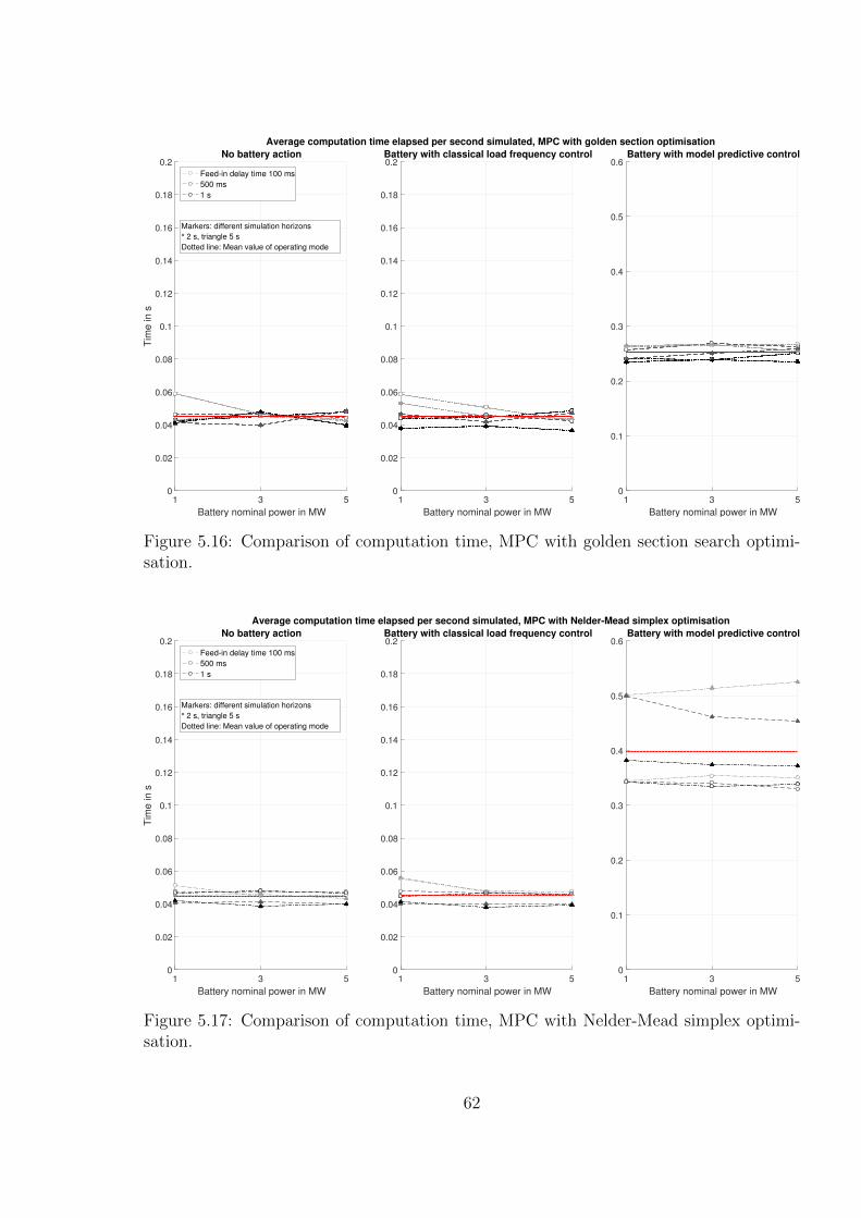
1 3 5

Battery nominal power in MW

0

0.02

0.04

0.06

0.08

0.1

0.12

0.14

0.16

0.18

0.2

Tim

e in

sNo battery action

Feed-in delay time 100 ms

500 ms

1 s

1 3 5

Battery nominal power in MW

0

0.02

0.04

0.06

0.08

0.1

0.12

0.14

0.16

0.18

0.2

Average computation time elapsed per second simulated, MPC with golden section optimisation

Battery with classical load frequency control

1 3 5

Battery nominal power in MW

0

0.1

0.2

0.3

0.4

0.5

0.6Battery with model predictive control

Markers: different simulation horizons

° 2 s, triangle 5 s

Dotted line: Mean value of operating mode

Figure 5.16: Comparison of computation time, MPC with golden section search optimi-sation.

1 3 5

Battery nominal power in MW

0

0.02

0.04

0.06

0.08

0.1

0.12

0.14

0.16

0.18

0.2

Tim

e in

s

No battery action

Feed-in delay time 100 ms

500 ms

1 s

1 3 5

Battery nominal power in MW

0

0.02

0.04

0.06

0.08

0.1

0.12

0.14

0.16

0.18

0.2

Average computation time elapsed per second simulated, MPC with Nelder-Mead simplex optimisation

Battery with classical load frequency control

1 3 5

Battery nominal power in MW

0

0.1

0.2

0.3

0.4

0.5

0.6Battery with model predictive control

Markers: different simulation horizons

° 2 s, triangle 5 s

Dotted line: Mean value of operating mode

Figure 5.17: Comparison of computation time, MPC with Nelder-Mead simplex optimi-sation.

62

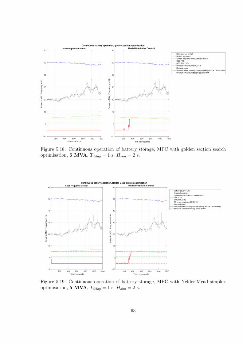
200 400 600 800 1000 1200

Time in seconds

-10

0

10

20

30

40

50

60

Pow

er

in M

W, F

requency in H

z

Load Frequency Control

200 400 600 800 1000 1200

Time in seconds

-10

0

10

20

30

40

50

60

Pow

er

in M

W, F

requency in H

z

Continuous battery operation, golden section optimisation

Model Predictive Control

Battery power in MW

System frequency

System frequency without battery action

SOC (*10)

SOC 50% (*10)

Minimum / maximum SOC (*10)

Demand power

Demand power, moving average (sliding window 100 seconds)

Minimum / maximum battery power in MW

Figure 5.18: Continuous operation of battery storage, MPC with golden section searchoptimisation, 5 MVA, Tdelay = 1 s, Hsim = 2 s.

200 400 600 800 1000 1200

Time in seconds

-10

0

10

20

30

40

50

60

Po

we

r in

MW

, F

req

ue

ncy in

Hz

Load Frequency Control

200 400 600 800 1000 1200

Time in seconds

-10

0

10

20

30

40

50

60

Po

we

r in

MW

, F

req

ue

ncy in

Hz

Continuous battery operation, Nelder-Mead simplex optimisation

Model Predictive Control

Battery power in MW

System frequency

System frequency without battery act on

SOC (*10)

SOC 50% (*10)

Minimum / maximum SOC (*10)

Demand power

Demand power, moving average (sliding window 100 seconds)

Minimum / maximum battery power in MW

Figure 5.19: Continuous operation of battery storage, MPC with Nelder-Mead simplexoptimisation, 5 MVA, Tdelay = 1 s, Hsim = 2 s.

63

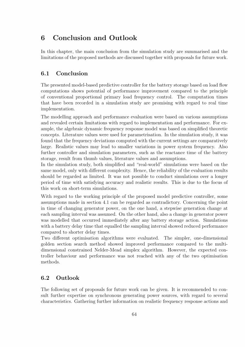
6 Conclusion and Outlook

In this chapter, the main conclusion from the simulation study are summarised and thelimitations of the proposed methods are discussed together with proposals for future work.

6.1 Conclusion

The presented model-based predictive controller for the battery storage based on load flowcomputations shows potential of performance improvement compared to the principleof conventional proportional primary load frequency control. The computation timesthat have been recorded in a simulation study are promising with regard to real timeimplementation.

The modelling approach and performance evaluation were based on various assumptionsand revealed certain limitations with regard to implementation and performance. For ex-ample, the algebraic dynamic frequency response model was based on simplified theoreticconcepts. Literature values were used for parametrisation. In the simulation study, it wasfound that the frequency deviations computed with the current settings are comparativelylarge. Realistic values may lead to smaller variations in power system frequency. Alsofurther controller and simulation parameters, such as the reactance time of the batterystorage, result from thumb values, literature values and assumptions.In the simulation study, both simplified and “real-world” simulations were based on thesame model, only with different complexity. Hence, the reliability of the evaluation resultsshould be regarded as limited. It was not possible to conduct simulations over a longerperiod of time with satisfying accuracy and realistic results. This is due to the focus ofthis work on short-term simulations.

With regard to the working principle of the proposed model predictive controller, someassumptions made in section 4.1 can be regarded as contradictory. Concerning the pointin time of changing generator power, on the one hand, a stepwise generation change ateach sampling interval was assumed. On the other hand, also a change in generator powerwas modelled that occurred immediately after any battery storage action. Simulationswith a battery delay time that equalled the sampling interval showed reduced performancecompared to shorter delay times.Two different optimisation algorithms were evaluated. The simpler, one-dimensionalgolden section search method showed improved performance compared to the multi-dimensional constrained Nelder-Mead simplex algorithm. However, the expected con-troller behaviour and performance was not reached with any of the two optimisationmethods.

6.2 Outlook

The following set of proposals for future work can be given. It is recommended to con-sult further expertise on synchronous generating power sources, with regard to severalcharacteristics. Gathering further information on realistic frequency response actions and

64

parameters would enable more accurate modelling approaches. Additionally, more in-formation on common practice and intervals of power changes in order to compensaterecorded load changes would be helpful for adjusting the system and frequency responsemodels.It should be considered to calculate frequency deviations caused by battery action only atthe next sampling time, corresponding to a battery delay times that equals the samplinginterval. For improved modelling of the battery storage, it would be interesting to includefeasible values for battery reaction time, sampling interval, possible intervals of batterypower changes.

With regard to performance evaluation of the control algorithm, the reliability of resultscould be improved by applying a more sophisticated, realistic model of the power system.Including secondary and optionally tertiary LFC, as well as interaction with neighbouringcontrol areas, may allow evaluations over longer periods of time.The computational speed of the controller and hence the controller performance may befurther enhanced by suitable technical solutions.

65

References

[1] U. EURELECTRIC, “Power distribution in europe, facts & figures,”EURELECTRIC,Union of the Electricity Industry, Tech. Rep., 2013.[Online]. Available: http://www.eurelectric.org/media/113155/dso report-webfinal-2013-030-0764-01-e.pdf

[2] A. J. Schwab, Elektroenergiesysteme, A. J. Schwab, Ed. Springer-VerlagGmbH, 2017. [Online]. Available: http://www.ebook.de/de/product/24473479/adolf j schwab elektroenergiesysteme.html

[3] B. Elia, “Electricity market players,” 2017. [Online]. Available: http://www.elia.be/en/about-elia/electricity-market-players

[4] E. N. o. T. S. O. ENTSO-E, “Ucte oh policy 1: Load-frequency control,” March2009. [Online]. Available: https://www.entsoe.eu/disclaimer/Pages/default.aspx

[5] ——, “Transmission system map,” 2015. [Online]. Available: https://www.entsoe.eu/map/Pages/default.aspx

[6] J. Arrillaga and C. P. Arnold, Computer Analysis of Power Systems. JOHN WI-LEY & SONS INC, 1991. [Online]. Available: http://www.ebook.de/de/product/3055885/jos arrillaga c p arnold computer analysis of power systems.html

[7] G. Andersson, “Modelling and analysis of electric power systems,” ETH Zurich,September 2008.

[8] Z. Kremens and M. Labuzek, “Load flow analysis incorporating frequency as a statevector variable,” in Harmonics and Quality of Power, 2000. Proceedings. NinthInternational Conference on, vol. 2. IEEE, 2000, pp. 526–530.

[9] Praviraj, “Newton-raphson loadflow,” 2009. [Online]. Available: https://de.mathworks.com/matlabcentral/fileexchange/21059-newton-raphson-loadflow

[10] P. M. Anderson and M. Mirheydar, “A low-order system frequency response model,”IEEE Transactions on Power Systems, vol. 5, no. 3, pp. 720–729, 1990.

[11] W. H. Kersting, “Ieee distribution planning working group report,” IEEE Trans.Power Syst, vol. 6, no. 3, pp. 975–985, 1991.

[12] IEEE, “Ieee pes distribution system analysis subcommittee’s distribution testfeeder working group,” 1991. [Online]. Available: http://ewh.ieee.org/soc/pes/dsacom/testfeeders/index.html

[13] U. UWEE, “Power systems test case archive,” University of Washington, Tech.Rep., 1993. [Online]. Available: http://www.ee.washington.edu/research/pstca/pf14/pg tca14bus.htm

66

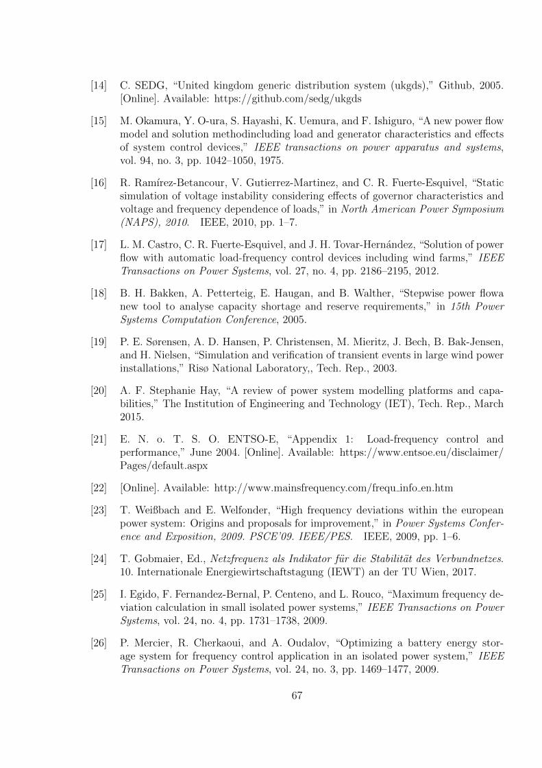
[14] C. SEDG, “United kingdom generic distribution system (ukgds),” Github, 2005.[Online]. Available: https://github.com/sedg/ukgds

[15] M. Okamura, Y. O-ura, S. Hayashi, K. Uemura, and F. Ishiguro, “A new power flowmodel and solution methodincluding load and generator characteristics and effectsof system control devices,” IEEE transactions on power apparatus and systems,vol. 94, no. 3, pp. 1042–1050, 1975.

[16] R. Ramırez-Betancour, V. Gutierrez-Martinez, and C. R. Fuerte-Esquivel, “Staticsimulation of voltage instability considering effects of governor characteristics andvoltage and frequency dependence of loads,” in North American Power Symposium(NAPS), 2010. IEEE, 2010, pp. 1–7.

[17] L. M. Castro, C. R. Fuerte-Esquivel, and J. H. Tovar-Hernandez, “Solution of powerflow with automatic load-frequency control devices including wind farms,” IEEETransactions on Power Systems, vol. 27, no. 4, pp. 2186–2195, 2012.

[18] B. H. Bakken, A. Petterteig, E. Haugan, and B. Walther, “Stepwise power flowanew tool to analyse capacity shortage and reserve requirements,” in 15th PowerSystems Computation Conference, 2005.

[19] P. E. Sørensen, A. D. Hansen, P. Christensen, M. Mieritz, J. Bech, B. Bak-Jensen,and H. Nielsen, “Simulation and verification of transient events in large wind powerinstallations,” Risø National Laboratory,, Tech. Rep., 2003.

[20] A. F. Stephanie Hay, “A review of power system modelling platforms and capa-bilities,” The Institution of Engineering and Technology (IET), Tech. Rep., March2015.

[21] E. N. o. T. S. O. ENTSO-E, “Appendix 1: Load-frequency control andperformance,” June 2004. [Online]. Available: https://www.entsoe.eu/disclaimer/Pages/default.aspx

[22] [Online]. Available: http://www.mainsfrequency.com/frequ info en.htm

[23] T. Weißbach and E. Welfonder, “High frequency deviations within the europeanpower system: Origins and proposals for improvement,” in Power Systems Confer-ence and Exposition, 2009. PSCE’09. IEEE/PES. IEEE, 2009, pp. 1–6.

[24] T. Gobmaier, Ed., Netzfrequenz als Indikator fur die Stabilitat des Verbundnetzes.10. Internationale Energiewirtschaftstagung (IEWT) an der TU Wien, 2017.

[25] I. Egido, F. Fernandez-Bernal, P. Centeno, and L. Rouco, “Maximum frequency de-viation calculation in small isolated power systems,” IEEE Transactions on PowerSystems, vol. 24, no. 4, pp. 1731–1738, 2009.

[26] P. Mercier, R. Cherkaoui, and A. Oudalov, “Optimizing a battery energy stor-age system for frequency control application in an isolated power system,” IEEETransactions on Power Systems, vol. 24, no. 3, pp. 1469–1477, 2009.

67

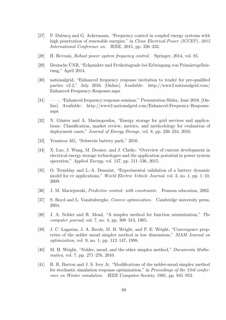
[27] P. Dubucq and G. Ackermann, “Frequency control in coupled energy systems withhigh penetration of renewable energies,” in Clean Electrical Power (ICCEP), 2015International Conference on. IEEE, 2015, pp. 326–332.

[28] H. Bevrani, Robust power system frequency control. Springer, 2014, vol. 85.

[29] Deutsche UNB, “Eckpunkte und Freiheitsgrade bei Erbringung von Primarregelleis-tung,” April 2014.

[30] nationalgrid, “Enhanced frequency response invitation to tender for pre-qualifiedparties v2.2,” July 2016. [Online]. Available: http://www2.nationalgrid.com/Enhanced-Frequency-Response.aspx

[31] ——, “Enhanced frequency response seminar,” Presentation Slides, June 2016. [On-line]. Available: http://www2.nationalgrid.com/Enhanced-Frequency-Response.aspx

[32] N. Gunter and A. Marinopoulos, “Energy storage for grid services and applica-tions: Classification, market review, metrics, and methodology for evaluation ofdeployment cases,” Journal of Energy Storage, vol. 8, pp. 226–234, 2016.

[33] Younicos AG, “Schwerin battery park,” 2016.

[34] X. Luo, J. Wang, M. Dooner, and J. Clarke, “Overview of current development inelectrical energy storage technologies and the application potential in power systemoperation,” Applied Energy, vol. 137, pp. 511–536, 2015.

[35] O. Tremblay and L.-A. Dessaint, “Experimental validation of a battery dynamicmodel for ev applications,” World Electric Vehicle Journal, vol. 3, no. 1, pp. 1–10,2009.

[36] J. M. Maciejowski, Predictive control: with constraints. Pearson education, 2002.

[37] S. Boyd and L. Vandenberghe, Convex optimization. Cambridge university press,2004.

[38] J. A. Nelder and R. Mead, “A simplex method for function minimization,” Thecomputer journal, vol. 7, no. 4, pp. 308–313, 1965.

[39] J. C. Lagarias, J. A. Reeds, M. H. Wright, and P. E. Wright, “Convergence prop-erties of the nelder–mead simplex method in low dimensions,” SIAM Journal onoptimization, vol. 9, no. 1, pp. 112–147, 1998.

[40] M. H. Wright, “Nelder, mead, and the other simplex method,” Documenta Mathe-matica, vol. 7, pp. 271–276, 2010.

[41] R. R. Barton and J. S. Ivey Jr, “Modifications of the nelder-mead simplex methodfor stochastic simulation response optimization,” in Proceedings of the 23rd confer-ence on Winter simulation. IEEE Computer Society, 1991, pp. 945–953.

68

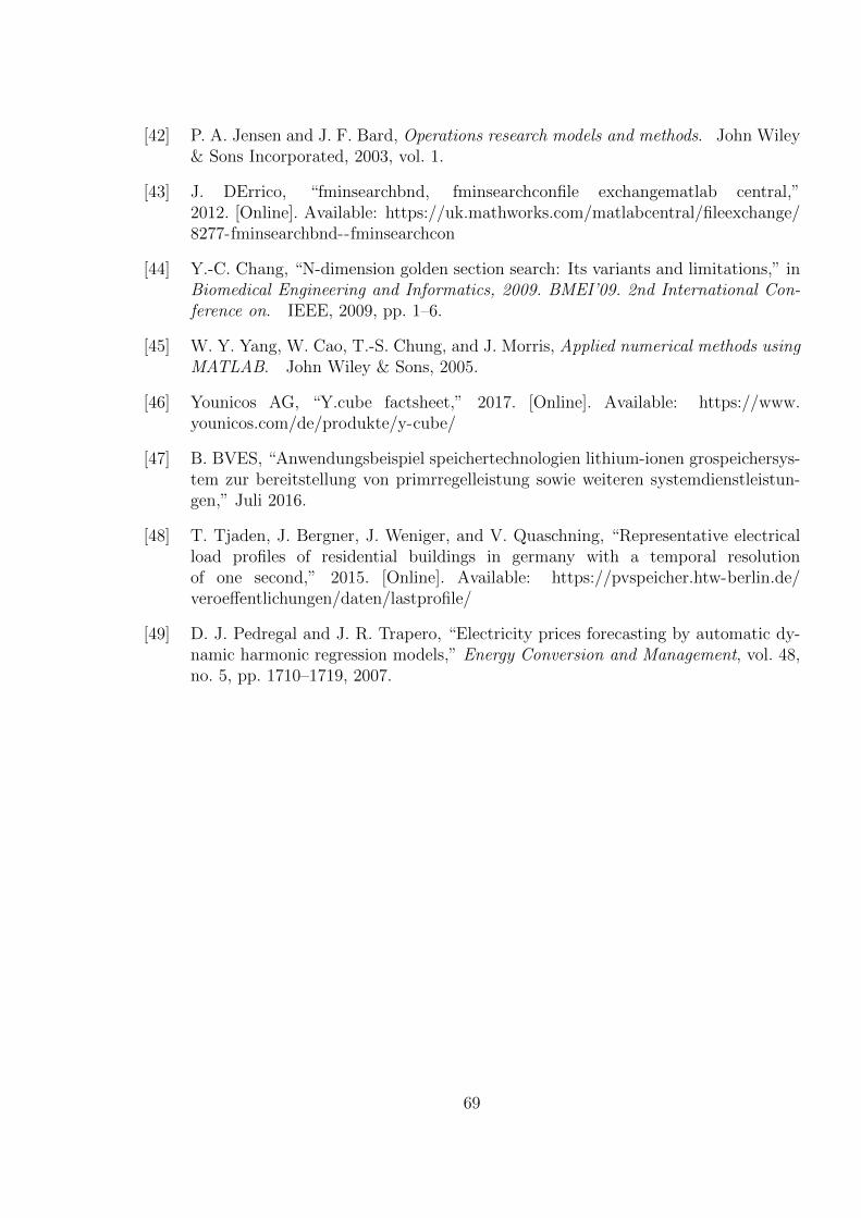
[42] P. A. Jensen and J. F. Bard, Operations research models and methods. John Wiley& Sons Incorporated, 2003, vol. 1.

[43] J. DErrico, “fminsearchbnd, fminsearchconfile exchangematlab central,”2012. [Online]. Available: https://uk.mathworks.com/matlabcentral/fileexchange/8277-fminsearchbnd--fminsearchcon

[44] Y.-C. Chang, “N-dimension golden section search: Its variants and limitations,” inBiomedical Engineering and Informatics, 2009. BMEI’09. 2nd International Con-ference on. IEEE, 2009, pp. 1–6.

[45] W. Y. Yang, W. Cao, T.-S. Chung, and J. Morris, Applied numerical methods usingMATLAB. John Wiley & Sons, 2005.

[46] Younicos AG, “Y.cube factsheet,” 2017. [Online]. Available: https://www.younicos.com/de/produkte/y-cube/

[47] B. BVES, “Anwendungsbeispiel speichertechnologien lithium-ionen grospeichersys-tem zur bereitstellung von primrregelleistung sowie weiteren systemdienstleistun-gen,” Juli 2016.

[48] T. Tjaden, J. Bergner, J. Weniger, and V. Quaschning, “Representative electricalload profiles of residential buildings in germany with a temporal resolutionof one second,” 2015. [Online]. Available: https://pvspeicher.htw-berlin.de/veroeffentlichungen/daten/lastprofile/

[49] D. J. Pedregal and J. R. Trapero, “Electricity prices forecasting by automatic dy-namic harmonic regression models,” Energy Conversion and Management, vol. 48,no. 5, pp. 1710–1719, 2007.

69