Modeling Simulationsof Autonomous,

Safety-Critical Systems

A Comparison between SCCharts and Ptolemy

Lars Peiler

Bachelor Thesis2015

Prof. Dr. von HanxledenReal-Time and Embedded SystemsDepartment of Computer Science

Kiel University

Advised byChristian Motika and Steven Smyth

Eidesstattliche Erklärung

Hiermit erkläre ich an Eides statt, dass ich die vorliegende Arbeit selbstständig verfasstund keine anderen als die angegebenen Quellen und Hilfsmittel verwendet habe.

Kiel,

iii

Abstract

Designing an embedded, safety-critical system is a difficult task. Since such a systemshould never fail under any circumstances, validation is advised. Simulations help to testa system in a safe environment before deploying the system to tests in the real world,therefore following a first-time-right approach that is important for safety-critical systems.

In the scope of a bachelor project, a quadcopter, a small, unmanned aerial vehiclewith four rotors, was designed, built and flown. This thesis covers a simulation that wasdesigned to represent the copter and to validate the flight controller. More specifically thismeans that the quadcopter should be able to fly without crashing by tilting too much inone direction and subsequently flying into a wall.

SCCharts is a visual language designed for specifying safety-critical reactive systemslike the quadcopter that uses KIEM to simulate the created model. SCCharts follows acontrol-flow oriented approach, an approach that focuses on the behavior of a system,yet offers data-flow as well. Data-flow focuses more on the flow of communication andcomputation between different parts of a model. This thesis will evaluate SCCharts andespecially data-flow in SCCharts as a means to design safety-critical systems and to createsimulations to execute these systems.

Key words modeling languages, SCCharts, Data-flow, Control-flow, Ptolemy, KIELER, KIEM,simulation, safety-critical system, quadcopter

v

Contents

1 Introduction 11.1 Sequentially Constructive Charts . . . . . . . . . . . . . . . . . . . . . . . . . 1

1.1.1 Data-flow in SCCharts . . . . . . . . . . . . . . . . . . . . . . . . . . . 31.2 KIELER Execution Manager . . . . . . . . . . . . . . . . . . . . . . . . . . . . . 41.3 The Quadcopter . . . . . . . . . . . . . . . . . . . . . . . . . . . . . . . . . . . 51.4 Problem Description . . . . . . . . . . . . . . . . . . . . . . . . . . . . . . . . 61.5 Outline . . . . . . . . . . . . . . . . . . . . . . . . . . . . . . . . . . . . . . . . 7

2 Related Work 92.1 Other Models and Simulations . . . . . . . . . . . . . . . . . . . . . . . . . . 92.2 Simulation and Modeling Tools . . . . . . . . . . . . . . . . . . . . . . . . . . 10

2.2.1 Matlab and Simulink . . . . . . . . . . . . . . . . . . . . . . . . . . . . 102.2.2 Safety Critical Application Development Environment . . . . . . . . 112.2.3 Testing in a Safe Environment . . . . . . . . . . . . . . . . . . . . . . 12

3 Used Technology 133.1 Ptolemy . . . . . . . . . . . . . . . . . . . . . . . . . . . . . . . . . . . . . . . . 13

3.1.1 KielerIO . . . . . . . . . . . . . . . . . . . . . . . . . . . . . . . . . . . 143.2 Kiel Integrated Environment for Layout Eclipse RichClient . . . . . . . . . . 143.3 Java Simple Serial Connector . . . . . . . . . . . . . . . . . . . . . . . . . . . 153.4 Arduino Mega 2560 . . . . . . . . . . . . . . . . . . . . . . . . . . . . . . . . . 16

4 Model and Simulation 174.1 Mathematical Model . . . . . . . . . . . . . . . . . . . . . . . . . . . . . . . . 17

4.1.1 Fundamental of the model . . . . . . . . . . . . . . . . . . . . . . . . 174.1.2 Rotation . . . . . . . . . . . . . . . . . . . . . . . . . . . . . . . . . . . 184.1.3 Linear Accelerations, Velocities and Position . . . . . . . . . . . . . . 204.1.4 Angular Velocities and Angles . . . . . . . . . . . . . . . . . . . . . . 214.1.5 Distance Calculation . . . . . . . . . . . . . . . . . . . . . . . . . . . . 234.1.6 Adjusting Output Values to the Quadcopter . . . . . . . . . . . . . . 244.1.7 Physical Properties of the Quadcopter . . . . . . . . . . . . . . . . . . 26

4.2 Simulating the Model . . . . . . . . . . . . . . . . . . . . . . . . . . . . . . . . 264.2.1 Simulating the Flight Controller . . . . . . . . . . . . . . . . . . . . . 284.2.2 Simulating the Model in KIELER Execution Manager (KIEM) . . . . . 29

vii

Contents

5 Realization 315.1 Realization with Ptolemy . . . . . . . . . . . . . . . . . . . . . . . . . . . . . 31

5.1.1 Linear Accelerations, Velocities and Position in Ptolemy . . . . . . . 325.1.2 Angular Velocities and Angles in Ptolemy . . . . . . . . . . . . . . . 335.1.3 Distance Calculation in Ptolemy . . . . . . . . . . . . . . . . . . . . . 345.1.4 Adjusting the Output Values in Ptolemy . . . . . . . . . . . . . . . . 36

5.2 Realization with SCCharts . . . . . . . . . . . . . . . . . . . . . . . . . . . . . 365.2.1 Linear Accelerations, Velocities and Position in SCCharts . . . . . . 375.2.2 Angular Velocities and Angles in SCCharts . . . . . . . . . . . . . . . 395.2.3 Distance Calculations in SCCharts . . . . . . . . . . . . . . . . . . . . 41

5.3 Simulating the Model . . . . . . . . . . . . . . . . . . . . . . . . . . . . . . . . 425.3.1 Ptolemy Data Component . . . . . . . . . . . . . . . . . . . . . . . . . 425.3.2 Communication between the Simulation and the Quadcopter . . . . 45

6 Evaluation 496.1 Results of the Simulation . . . . . . . . . . . . . . . . . . . . . . . . . . . . . . 49

6.1.1 Problems with the simulation . . . . . . . . . . . . . . . . . . . . . . . 496.2 Comparison between Ptolemy and SCCharts . . . . . . . . . . . . . . . . . . 50

6.2.1 Implementation Differences . . . . . . . . . . . . . . . . . . . . . . . . 506.2.2 Differences in Calculations . . . . . . . . . . . . . . . . . . . . . . . . 52

6.3 Encountered Problems . . . . . . . . . . . . . . . . . . . . . . . . . . . . . . . 536.3.1 Problems Encountered using Ptolemy . . . . . . . . . . . . . . . . . . 536.3.2 Problems Encountered using SCCharts . . . . . . . . . . . . . . . . . 54

7 Conclusion 577.1 Summary . . . . . . . . . . . . . . . . . . . . . . . . . . . . . . . . . . . . . . . 577.2 Future Work . . . . . . . . . . . . . . . . . . . . . . . . . . . . . . . . . . . . . 57

7.2.1 Future Work on the Simulation . . . . . . . . . . . . . . . . . . . . . . 587.2.2 Future Work on Data-Flow . . . . . . . . . . . . . . . . . . . . . . . . 59

Bibliography 61

Instructions for the Simulation 65.1 Simulating without the Arduino . . . . . . . . . . . . . . . . . . . . . . . . . 65.2 Simulating with the Arduino . . . . . . . . . . . . . . . . . . . . . . . . . . . 65.3 Changing the Models . . . . . . . . . . . . . . . . . . . . . . . . . . . . . . . . 66

viii

List of Figures

1.1 Core and Extended SCCharts . . . . . . . . . . . . . . . . . . . . . . . . . . . 21.2 Difference between a falling ball in a control-flow and a data-flow oriented

modeling language . . . . . . . . . . . . . . . . . . . . . . . . . . . . . . . . . 31.3 Bouncing Ball – heterogeneous model . . . . . . . . . . . . . . . . . . . . . . 41.4 Data-flow in SCCharts . . . . . . . . . . . . . . . . . . . . . . . . . . . . . . . 41.5 The KIEM interface . . . . . . . . . . . . . . . . . . . . . . . . . . . . . . . . . 51.6 Schematic layout of the quadcopter . . . . . . . . . . . . . . . . . . . . . . . 7

2.1 Simulation GUI of Matlab/Simulink . . . . . . . . . . . . . . . . . . . . . . . 102.2 GUI of the Safety Critical Application Development Environment (SCADE)

Suite . . . . . . . . . . . . . . . . . . . . . . . . . . . . . . . . . . . . . . . . . 11

3.1 Ptolemy GUI . . . . . . . . . . . . . . . . . . . . . . . . . . . . . . . . . . . . . 143.2 Overview over the Kiel Integrated Environment for Layout Eclipse Rich-

Client (KIELER) project . . . . . . . . . . . . . . . . . . . . . . . . . . . . . . . 15

4.1 The different frames of the quadcopter . . . . . . . . . . . . . . . . . . . . . 184.2 The axes of the gyroscope on the quadcopter . . . . . . . . . . . . . . . . . . 204.3 Distance measurement of a quadcopter . . . . . . . . . . . . . . . . . . . . . 234.4 Distance measurement of the quadcopter dismissing the closest wall . . . . 254.5 Component diagram . . . . . . . . . . . . . . . . . . . . . . . . . . . . . . . . 274.6 Class diagram . . . . . . . . . . . . . . . . . . . . . . . . . . . . . . . . . . . . 27

5.2 Calculating the torque of the quadcopter in Ptolemy . . . . . . . . . . . . . 325.3 Calculating the acceleration in the inertial frame in Ptolemy . . . . . . . . . 335.4 Calculating the drag affecting the quadcopter in Ptolemy . . . . . . . . . . . 335.5 Calculating the angles in Ptolemy . . . . . . . . . . . . . . . . . . . . . . . . 345.6 Calculating the angular accelerations in Ptolemy . . . . . . . . . . . . . . . . 355.7 The modal model describing the current direction of the quadcopter in

Ptolemy . . . . . . . . . . . . . . . . . . . . . . . . . . . . . . . . . . . . . . . . 355.8 Calculating the distances to the walls in Ptolemy . . . . . . . . . . . . . . . 365.9 Calculating the thrust in SCCharts . . . . . . . . . . . . . . . . . . . . . . . . 375.10 Calculating the accelerations in SCCharts . . . . . . . . . . . . . . . . . . . . 375.11 Calculating the output accelerations in SCCharts . . . . . . . . . . . . . . . . 385.12 Calculating the velocity and the position in SCCharts . . . . . . . . . . . . . 39

ix

List of Figures

5.13 Calculating the angular velocities in SCCharts . . . . . . . . . . . . . . . . . 405.14 Calculating the current angles in SCCharts . . . . . . . . . . . . . . . . . . . 405.15 Calculating the distances between the walls and the quadcopter in SCCharts 415.16 Class diagram . . . . . . . . . . . . . . . . . . . . . . . . . . . . . . . . . . . . 42

6.1 A very cluttered and unclear part of the model in SCCharts . . . . . . . . . 516.2 Data-flow divided into different regions . . . . . . . . . . . . . . . . . . . . . 526.3 Data-flow divided into different nested SCCharts . . . . . . . . . . . . . . . 526.4 Redundant information in data-flow . . . . . . . . . . . . . . . . . . . . . . . 556.5 Hostcode in SCCharts data-flow . . . . . . . . . . . . . . . . . . . . . . . . . 566.6 Cluttered inner node with too much text . . . . . . . . . . . . . . . . . . . . 56

7.1 Example diagram for the outputs . . . . . . . . . . . . . . . . . . . . . . . . . 587.2 3D representation of the quadcopter in a room . . . . . . . . . . . . . . . . . 59

x

Abbreviations

EECS Electrical Engineering and Computer Sciences

JSON JavaScript Object Notation

JSSC Java Simple Serial Connector

KEV KIELER Environment Visualization

KIELER Kiel Integrated Environment for Layout Eclipse RichClient

KIEM KIELER Execution Manager

LGPL Lesser General Public License

M2M Model-to-Model

MoC Model of Computation

RTSYS Real-Time and Embedded Sytems

SI Système international d’unités

SCADE Safety Critical Application Development Environment

SCT SCCharts Text

xi

Chapter 1

Introduction

Safety-critical systems, such as systems used in the automotive or aerospace industry,are difficult to design. Only one small, faulty part of the system can lead to unforeseencircumstances or crashes and could therefore even cause injuries or worse to humans.

Traditional programming languages and practices generally have problems designingthese systems due to unpredictability or the lack of overview. Some scientists like Leeadvise against threads as a means to model or create concurrency as non-determinismin programming is fairly dangerous and should be handled explicitly [Lee06]. Therefore,different modeling tools like Ptolemy as well as synchronous languages such as Esterelor Lustre are often used to model and design such systems [BCE+03]. These tools takean approach to eliminate race conditions and therefore ensure deterministic behavior.Ptolemy in particular qualifies especially for the simulation of environments due to itsheterogeneous approach to modeling. On the other hand, SCCharts, as described below, isa modeling language designed to model reactive systems yet struggles to describe modelsfor environments of bigger physical systems [Uml15]. Recently, SCCharts underwentdevelopment in the direction of simulations with the implementation of data-flow. Thefocus of this thesis now lies on the comparison between Ptolemy and SCCharts as tools forthe creation of models on the basis of a model of a quadcopter. The paper will evaluate thepossibilities of further development in SCCharts to create a better tool for the creation ofsimulations and models of environments.

Before going into more detail, the introduction gives a short overview over the mostimportant parts of this thesis: The core modeling technology in SCCharts as well as thesimulation tool and the quadcopter itself. Finally, this chapter describes the main problemthis thesis focuses on and the general outline of the paper.

1.1 Sequentially Constructive Charts

SCCharts, as introduced by von Hanxleden et al. from the Real-Time and EmbeddedSytems (RTSYS) group at the Kiel University [HDM+14], is a visual synchronous languagedesigned for specifying safety-critical reactive systems. SCCharts uses a statechart notationsimilar to the one used by Harel in his Statecharts approach [Har87]. While SCChartsprovides deterministic concurrency based on a synchronous Model of Computation (MoC)

1

1. Introduction

Interface

declaration

Final state

Connector

Initial state

Root state

Named

simple state

Transition

trigger/effect

Region ID

Transition

priority

Conditional

termination

Anonymous

simple state

History transition

Entry/During/Exit

actions

Termination

Superstate

Signal

Immediate

transition

Suspension

Strong abort

Local declaration

Weak abort

Deferred transition

Count Delay

Pre-Operator

Initialization

Complex final

state

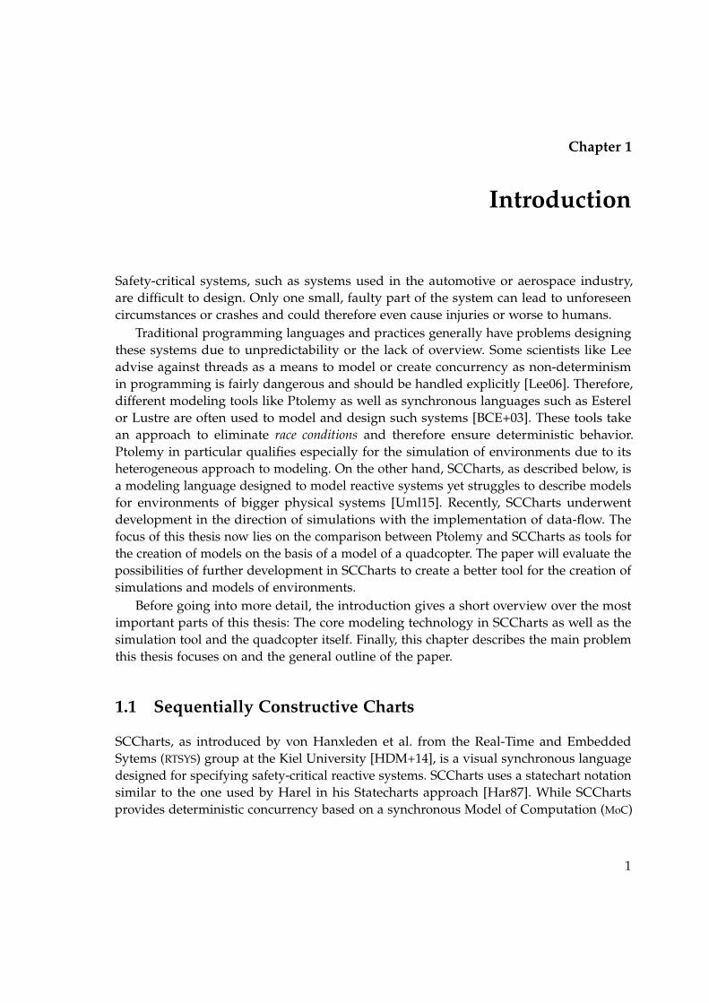
Figure 1.1. Features of Core and Extended SCCharts [HDM+14]

as introduced by Berry [BB91], it also allows emitting different values of a signal (orvariable) within one tick as long as the program stays sequentially schedulable. This socalled Sequentially Constructive MoC as introduced by von Hanxleden et al. now allowssome more programming paradigms while keeping the program deterministic [HMA+13].

SCCharts can be divided into two different parts: Core SCCharts and Extended SCCha-rts. Core SCCharts contain a minimal amount of elements that is able to express everythingthe Sequentially Constructive MoC requires, such as states, transitions and hierarchies.Extended SCCharts is built upon Core SCCharts, simplifies a magnitude of elements andadds syntactical sugar. Figure 1.1 shows the different elements of Core and Extended SC-Charts. Every additional feature can be translated to equivalent features in Core SCChartsvia semantics preserving Model-to-Model (M2M) transformations [HMA+13]. In SCChartsthe modeller typically designs the models with the textual language SCCharts Text (SCT).It is a language based on an Xtext grammar, thus allowing content-assist to simplify the

2

1.1. Sequentially Constructive Charts

process. Xtext1 is a framework for development of programming languages and domainspecific languages. With SCT the user designs a textual model which is then step for stepsynthesised into a graphical model as well as compilable C code or other code.

1.1.1 Data-flow in SCCharts

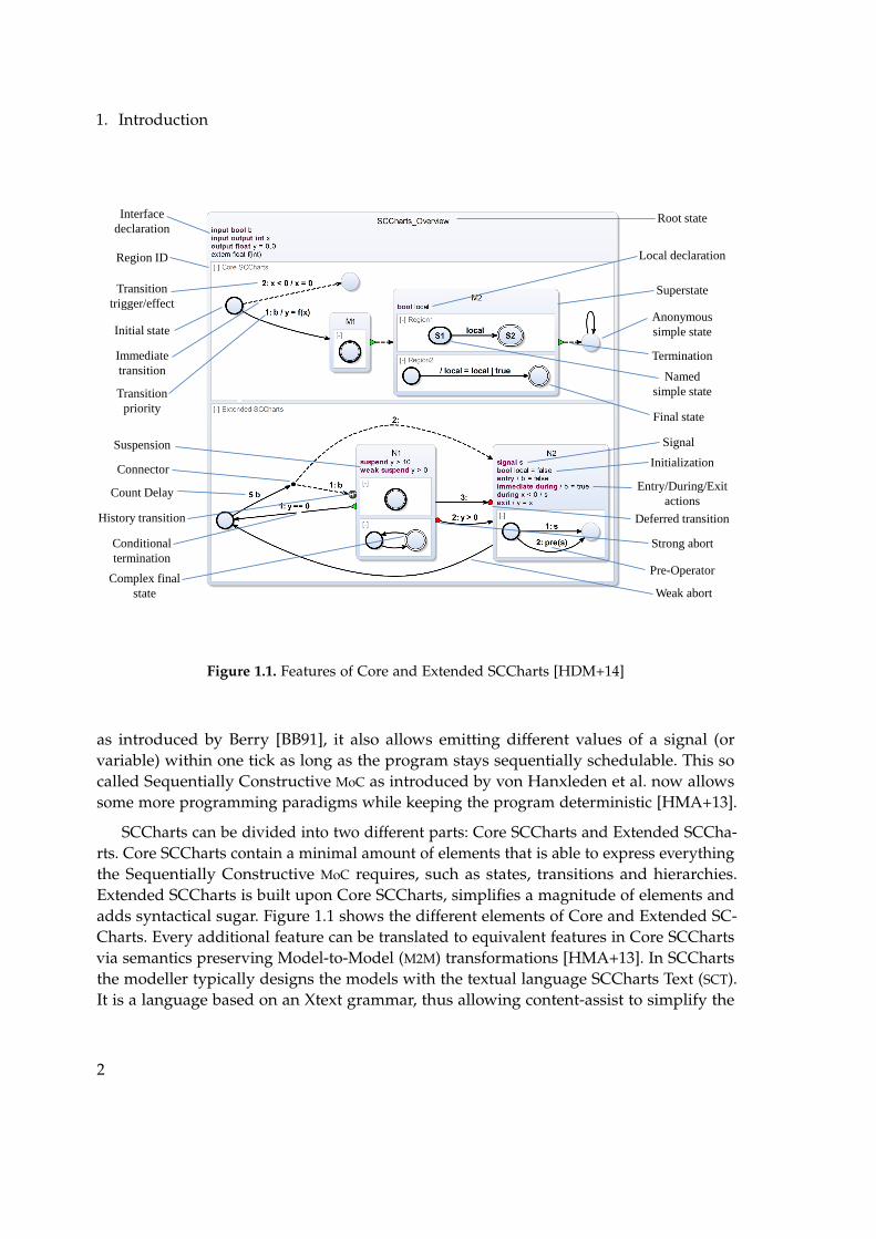
As a derivative of SyncCharts by André [And96], SCCharts was developed with control-flow in mind, using hierarchical, synchronous state machines. Control-flow focuses ondescriptions of the behavior of a system. Therefore, control-flow is often visualized usingstate machines. On the other hand, when trying to compute variables, where the commu-nication between the different components of the model, the so called actors, is a moreimportant aspect, using a data-flow environment might be of advantage [Uml15; CPP05].For example, to describe a falling ball, a state machine like the one in Figure 1.2a failsto clarify the situation appropriately even in such a small example while the data-floworiented approach in figure Figure 1.2b is much easier to follow for an outsider.

FallingBall const float gravity = 9.81const float time = 0.02output float velocityoutput float position

[-]init

falling during / velocity = velocity + gravity * timeduring / position = position + velocity * time

(a) A falling ball modeled in SCCharts(b) A falling ball modeled in Ptolemy

Figure 1.2. Difference between a falling ball in a control-flow and a data-flow oriented modelinglanguage

Furthermore, not every model can be completely associated with either data-flowor control-flow. For example, if the same falling ball from above hits the ground, itexperiences acceleration upwards. This sudden change in the state of the ball can beexpressed using different states. In that case, a hybrid system using both concepts isadvantageous. Figure 1.3 shows a hybrid system in Ptolemy describing the mentionedsituation.

As evident, hybrid systems can express many situations more clearly. Therefore, data-flow in SCCharts was introduced by Umland [Uml15]. It creates a way to use data-flow

1http://www.eclipse.org/Xtext/

3

1. Introduction

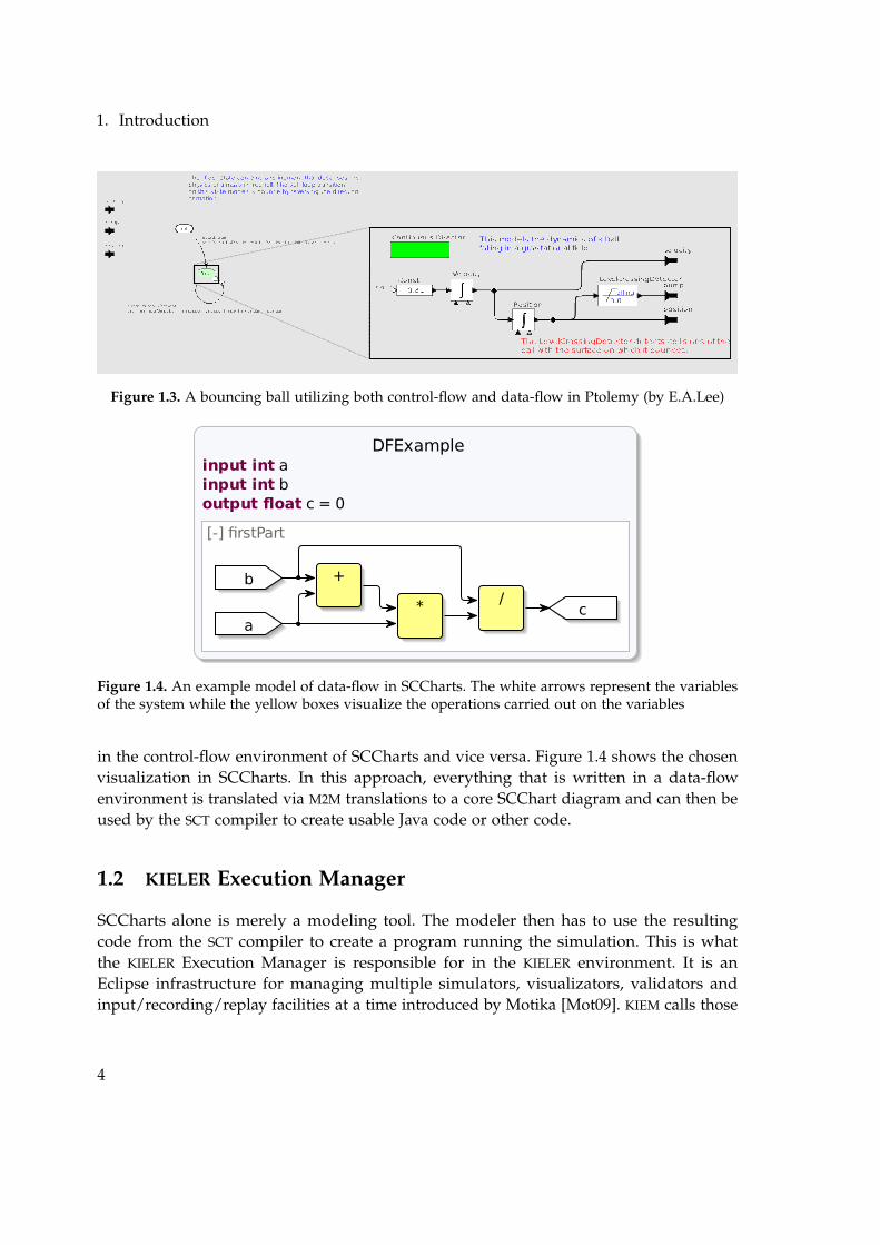
Figure 1.3. A bouncing ball utilizing both control-flow and data-flow in Ptolemy (by E.A.Lee)

DFExample input int ainput int boutput float c = 0

[-] firstPart

a

b +

* /c

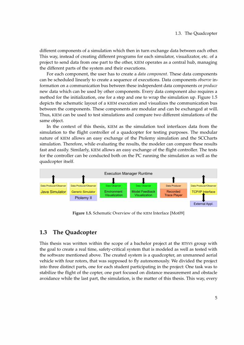
Figure 1.4. An example model of data-flow in SCCharts. The white arrows represent the variablesof the system while the yellow boxes visualize the operations carried out on the variables

in the control-flow environment of SCCharts and vice versa. Figure 1.4 shows the chosenvisualization in SCCharts. In this approach, everything that is written in a data-flowenvironment is translated via M2M translations to a core SCChart diagram and can then beused by the SCT compiler to create usable Java code or other code.

1.2 KIELER Execution Manager

SCCharts alone is merely a modeling tool. The modeler then has to use the resultingcode from the SCT compiler to create a program running the simulation. This is whatthe KIELER Execution Manager is responsible for in the KIELER environment. It is anEclipse infrastructure for managing multiple simulators, visualizators, validators andinput/recording/replay facilities at a time introduced by Motika [Mot09]. KIEM calls those

4

1.3. The Quadcopter

different components of a simulation which then in turn exchange data between each other.This way, instead of creating different programs for each simulator, visualizator, etc. of aproject to send data from one part to the other, KIEM operates as a central hub, managingthe different parts of the system and their executions.

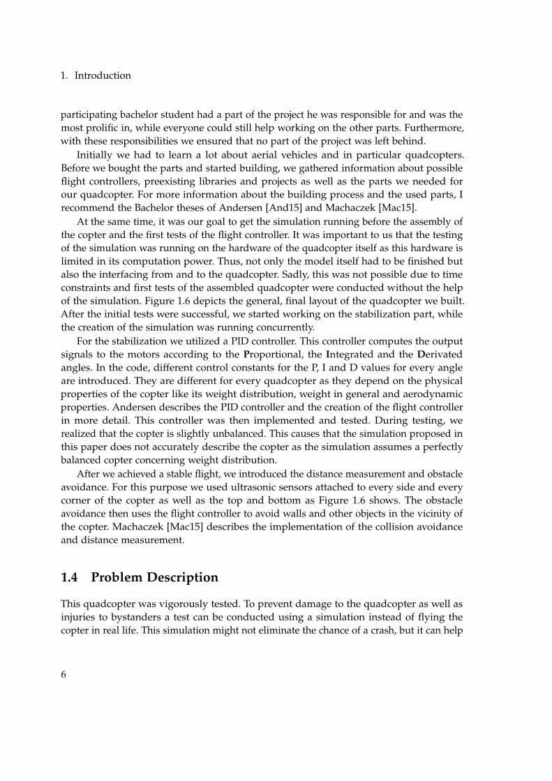
For each component, the user has to create a data component. These data componentscan be scheduled linearly to create a sequence of executions. Data components observe in-formation on a communication bus between these independent data components or producenew data which can be used by other components. Every data component also requires amethod for the initialization, one for a step and one to wrap the simulation up. Figure 1.5depicts the schematic layout of a KIEM execution and visualizes the communication busbetween the components. These components are modular and can be exchanged at will.Thus, KIEM can be used to test simulations and compare two different simulations of thesame object.

In the context of this thesis, KIEM as the simulation tool interfaces data from thesimulation to the flight controller of a quadcopter for testing purposes. The modularnature of KIEM allows an easy exchange of the Ptolemy simulation and the SCChartssimulation. Therefore, while evaluating the results, the modeler can compare these resultsfast and easily. Similarly, KIEM allows an easy exchange of the flight controller. The testsfor the controller can be conducted both on the PC running the simulation as well as thequadcopter itself.

Execution Manager Runtime

Java Simulator

Data Producer/Observer

Generic Simulator

Data Producer/Observer

Ptolemy II

Environment Visualization

Data Observer

Model FeedbackVisualization

Data Observer

RecordedTrace Player

Data Producer

TCP/IP Interface

Data Producer/Observer

External Appl.

Figure 1.5. Schematic Overview of the KIEM Interface [Mot09]

1.3 The Quadcopter

This thesis was written within the scope of a bachelor project at the RTSYS group withthe goal to create a real time, safety-critical system that is modeled as well as tested withthe software mentioned above. The created system is a quadcopter, an unmanned aerialvehicle with four rotors, that was supposed to fly autonomously. We divided the projectinto three distinct parts, one for each student participating in the project: One task was tostabilize the flight of the copter, one part focused on distance measurement and obstacleavoidance while the last part, the simulation, is the matter of this thesis. This way, every

5

1. Introduction

participating bachelor student had a part of the project he was responsible for and was themost prolific in, while everyone could still help working on the other parts. Furthermore,with these responsibilities we ensured that no part of the project was left behind.

Initially we had to learn a lot about aerial vehicles and in particular quadcopters.Before we bought the parts and started building, we gathered information about possibleflight controllers, preexisting libraries and projects as well as the parts we needed forour quadcopter. For more information about the building process and the used parts, Irecommend the Bachelor theses of Andersen [And15] and Machaczek [Mac15].

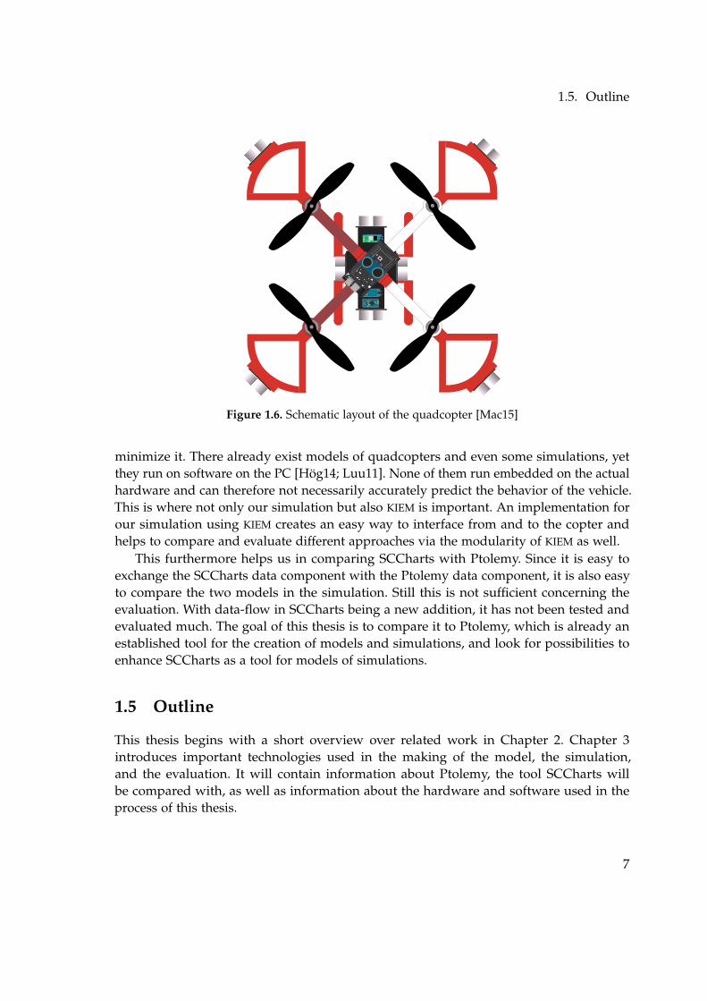
At the same time, it was our goal to get the simulation running before the assembly ofthe copter and the first tests of the flight controller. It was important to us that the testingof the simulation was running on the hardware of the quadcopter itself as this hardware islimited in its computation power. Thus, not only the model itself had to be finished butalso the interfacing from and to the quadcopter. Sadly, this was not possible due to timeconstraints and first tests of the assembled quadcopter were conducted without the helpof the simulation. Figure 1.6 depicts the general, final layout of the quadcopter we built.After the initial tests were successful, we started working on the stabilization part, whilethe creation of the simulation was running concurrently.

For the stabilization we utilized a PID controller. This controller computes the outputsignals to the motors according to the Proportional, the Integrated and the Derivatedangles. In the code, different control constants for the P, I and D values for every angleare introduced. They are different for every quadcopter as they depend on the physicalproperties of the copter like its weight distribution, weight in general and aerodynamicproperties. Andersen describes the PID controller and the creation of the flight controllerin more detail. This controller was then implemented and tested. During testing, werealized that the copter is slightly unbalanced. This causes that the simulation proposed inthis paper does not accurately describe the copter as the simulation assumes a perfectlybalanced copter concerning weight distribution.

After we achieved a stable flight, we introduced the distance measurement and obstacleavoidance. For this purpose we used ultrasonic sensors attached to every side and everycorner of the copter as well as the top and bottom as Figure 1.6 shows. The obstacleavoidance then uses the flight controller to avoid walls and other objects in the vicinity ofthe copter. Machaczek [Mac15] describes the implementation of the collision avoidanceand distance measurement.

1.4 Problem Description

This quadcopter was vigorously tested. To prevent damage to the quadcopter as well asinjuries to bystanders a test can be conducted using a simulation instead of flying thecopter in real life. This simulation might not eliminate the chance of a crash, but it can help

6

1.5. Outline

VCC

GND

TX

RX

Ard

uino

Pro

Min

i

Res

et

98765432GNDRSTRXITXO

TXO

RX

I

RAW GND RST VCC A3 A2 A1 A0 13 12 11 10

VC

CG

ND

BLK

GRN

C106

C106

L

RESET

RXTX

01

23

45

67

89

10

11

12

13

A0A1

A2A3

A4A5

6A7

A8A9

A10A11

A12A13

A14A15

22

24

26

28

30

31

32

33

34

35

36

37

38

39

41

40

43

42

45

47

49

MOSI

44

46

MISO

48SS

SCK

ANALOG IN

COMMUNICATIO

N

AREFGND

TX0 RX0

Arduino

RESET 3V3

5V

VIN

GND

GND

SDA 20 SCL 21

1

TX2 16 RX2 1

7

RX3 15

TX3 14

RX1 19

TX1 18

PWM

5V

GND

DIGITA

L

MEGA

IOREF

ON

Figure 1.6. Schematic layout of the quadcopter [Mac15]

minimize it. There already exist models of quadcopters and even some simulations, yetthey run on software on the PC [Hög14; Luu11]. None of them run embedded on the actualhardware and can therefore not necessarily accurately predict the behavior of the vehicle.This is where not only our simulation but also KIEM is important. An implementation forour simulation using KIEM creates an easy way to interface from and to the copter andhelps to compare and evaluate different approaches via the modularity of KIEM as well.

This furthermore helps us in comparing SCCharts with Ptolemy. Since it is easy toexchange the SCCharts data component with the Ptolemy data component, it is also easyto compare the two models in the simulation. Still this is not sufficient concerning theevaluation. With data-flow in SCCharts being a new addition, it has not been tested andevaluated much. The goal of this thesis is to compare it to Ptolemy, which is already anestablished tool for the creation of models and simulations, and look for possibilities toenhance SCCharts as a tool for models of simulations.

1.5 Outline

This thesis begins with a short overview over related work in Chapter 2. Chapter 3introduces important technologies used in the making of the model, the simulation,and the evaluation. It will contain information about Ptolemy, the tool SCCharts willbe compared with, as well as information about the hardware and software used in theprocess of this thesis.

7

1. Introduction

In Chapter 4, the physical model will be described in detail. The chapter will give insightinto the different aspects of the model such as the rotational matrices, how to calculatethe acceleration, velocity and position as well as the angular velocities. Additionally,the reasons for the use of KIEM as the simulation tool will be explained in more detail.Afterwards, in Chapter 5, the realization of the model in both Ptolemy and in SCCharts isdelineated. Both of these sections will cover the same model realized on different platforms.Furthermore, this chapter will deal with the implementation of the simulation and how themodels have been tested. A short section about calculations for some physical propertiesof the quadcopter will close the chapter.

Chapter 6 will evaluate the two approaches and will compare the advantages anddisadvantages of those. It will give insight into the creation of the models in the differenttools and the problems encountered. The chapter will further describe the differences inthe calculation, as the two tools are inherently different in their computations.

The final chapter covers the conclusion, lessons learned in Ptolemy and SCCharts aswell as some suggestions for future work in SCCharts, especially data-flow in SCCharts.

8

Chapter 2

Related Work

This chapter covers other scientific papers and related work. First, it addresses papers thatare also about the simulation and modeling of a quadcopter. Following that, the chapterdescribes different software that could be considered for the creation of a model or asimulation for a quadcopter or a similar vehicle.

2.1 Other Models and Simulations

There have already been multiple papers and theses describing physical properties andmodels of quadcopters of different sizes. These physical properties are fairly well under-stood and are described in a multitude of papers.

Höger [Hög14] describes the model of quadcopters in general and then adapts thismodel to the Crazyflie1, a very small quadcopter for indoor use. His work is more con-densed concerning the model and focuses more on the mathematical backgrounds of thecalculations and the adaptation required for the Crazyflie. Thus, he concentrates a lot ondetermining unknown constants of the quadcopter. His approach to finding these valuesis very complex and doing a similar approach would go beyond the scope of this thesis.Therefore, only the model and information about the rotational matrices were taken fromthis thesis. Höger uses Matlab as the modeling and simulation environment. Thusly, thecalculations do not run in the native code the hardware of the copter requires. This couldpossibly lead to unexpected behavior if the code is finally running on the copter as it isnot tested, because of the speed of the hardware or because of differences in the nativelanguage.

Another approach to model a generic quadcopter has been done by Luukkonen [Luu11].He describes the physical model of the quadcopter in more detail and furthermore givesinsight into his method for controlling the copter. His approach was never tested in reality.Furthermore, he uses values to input into his simulation that a common quadcopter cannotaccurately measure such as the current velocity as an input to the copter. The coptermight be able to calculate his velocity with the help of the accelerometer, but commonaccelerometers are not very exact and often output noise. He also uses Matlab as themodeling and simulation environment.

1https://www.bitcraze.io/crazyflie-2/

9

2. Related Work

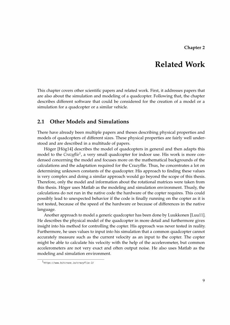
Figure 2.1. The simulation GUI of Matlab/Simulink [Mot07]

McGilvray and Tayebi describe the physical properties of a quadcopter in their paperAttitude stabilization of a four-rotor aerial robot [TM04]. Furthermore, they show a small partof their simulation results using their model and the corresponding PID controller. Sincemany physical properties of a quadcopter are hard to determine, the simulation in thisthesis uses the properties of the quadcopter described by McGilvray. Therefore it is hard toapply the simulation results to the quadcopter that was built for the project of this thesis.

2.2 Simulation and Modeling Tools

Since one big part of this thesis is the evaluation of SCCharts as a modeling environmentand simulation tool for data-flow oriented models, it is also important to consider differentcomparison tools. For this purpose, Ptolemy, as described in more detail in Chapter 3,was chosen due to the preexisting integration in KIEM and the ease to create heteroge-neous models, which simulations often times require. However, other tools should stillbe considered. This section covers some popular tools that are used to design and modelsimulations.

2.2.1 Matlab and Simulink

Both Höger and Luukkonen use Matlab2 as a tool for both modeling and simulating theirapproach. Matlab is a programming language designed specifically with mathematicalsystems in mind. This includes data-flow oriented systems like the physical model of aquadcopter. Matlab also allows for very clear visualizations of simulation results. As such,it is very qualified for the purpose of this paper. However, Matlab lacks when it comes

2http://www.mathworks.com/products/matlab/

10

2.2. Simulation and Modeling Tools

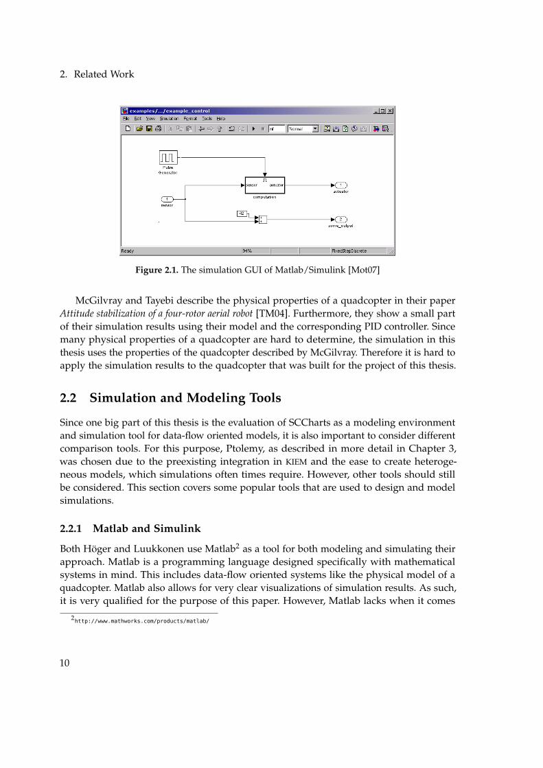
Figure 2.2. The GUI and an example project in the SCADE Suite5

to usability and is definitely neither beginner friendly nor clear when modeling biggersystems. Therefore, Matlab alone was not considered. Simulink3, as depicted in Figure 2.1,extends Matlab with a visualization and a graphical editing tool for data-flow models. Itsimplifies a lot of the problems Matlab alone struggles with mentioned above. However,the integration of Matlab and Simulink into KIEM is difficult as a stepwise execution ofmodels is only possible after computing complete results. This means that a real-timeexecution of the simulation is not possible in Simulink. Therefore, it is impossible forMatlab and Simulink to react to the behavior of the flight controller, if the flight controlleris not written in Matlab as well. Since we were already experienced with SCCharts as wellas Ptolemy, we chose to disregard Matlab. Another reason against Matlab and Simulinkand for SCCharts and Ptolemy is that SCCharts and Ptolemy are open source while Matlabis a commercial product that is not open source.

2.2.2 Safety Critical Application Development Environment

The SCADE Suite4, as depicted in Figure 2.2, is a model-based development environmentfor critical embedded software. Modelers can design their model both graphically aswell as textually with SCADE, which can then generate C or ADA code from these models.Motika [Mot07] uses this tool to design a simulation for a model railway that is supposed to

3http://www.mathworks.com/products/simulink/5Source: http://www.esterel-technologies.com/wp-content/uploads/2015/03/SCADE-Suite-IDE-View.png4http://www.esterel-technologies.com/products/scade-suite/

11

2. Related Work

control multiple trains on different tracks and courses. Since KIEM was chosen to simulatethe model and SCADE interfaces using the Transmission Control Protocol (TCP) whichcomplicates the communication, SCADE was not considered as an alternative to Ptolemy.Since SCADE is also not open source, another way to integrate the tool into a work-flow isnot possible.

2.2.3 Testing in a Safe Environment

Multiple studies with quadcopters were conducted in a safe environment instead of usinga simulation. One such approach is described by Castillo et al. [CLD05]. However, therequired hardware for the testing environment was not available. Furthermore, in the testsconducted in the scope of this thesis, it was noticed, that a cable attached to the copterinfluences his flying capabilities severely.

The project still used a lot of live testing without this testing environment to test theactual capabilities of the quadcopter. These tests were conducted without an environmentlike the one mentioned above and will not be a part of this thesis.

12

Chapter 3

Used Technology

Prior to explaining the model of the quadcopter, it is necessary to sketch the importantused technologies in the making of this thesis. This chapter contains information about atool used to create a model that compares to the one created in SCCharts, more generalinformation about the KIELER project as well as technology used for the exchange ofinformation to and from the quadcopter and the hardware on the quadcopter.

3.1 Ptolemy

The Ptolemy Project1 is an open-source, Java based tool for designing and simulatingconcurrent, real-time, embedded systems as introduced by [Lee03]. Ptolemy II, hereafterjust Ptolemy, is in development by the Electrical Engineering and Computer Sciences (EECS)faculty at UC Berkeley since 1996. This tool simplifies the creation of complex models withhierarchical structures and an actor-oriented design. Actors are concurrently executingsoftware components that, when interconnected via ports, send messages to other actorsand thus make up a model. The behavior of every actor is described in its Java class andranges from simple mathematical operations like adding and subtracting to complex oneslike integration.

A Ptolemy model is stored in an XML-file. Thus, a user can easily extract informationif he wants to. The semantics of a model is determined by its director – a componentimplementing a model of computation. Each level in the hierarchy of the model can haveits own director, and understanding these directors and their interactions is a core partin the creation of different models with Ptolemy. These different directors allow differentapproaches to modeling such as a data-flow oriented or a control-flow oriented approach.Heterogeneous combinations of directors enable the modeler to design the model he or shewants to create. An example for this heterogeneous approach is the use of a synchronousreactive director, a director using a data-flow oriented approach, in combination witha modal model, a control-flow oriented director, that is hierarchically embedded in themodel with the synchronous reactive director, creating a StateChart [Pto14].

Vergil, the UI of Ptolemy, visualizes the model as seen in Figure 3.1 and allows themodeler to easily edit the model. The user controls the tool by drag-and-drop and can edit

1http://ptolemy.eecs.berkeley.edu/

13

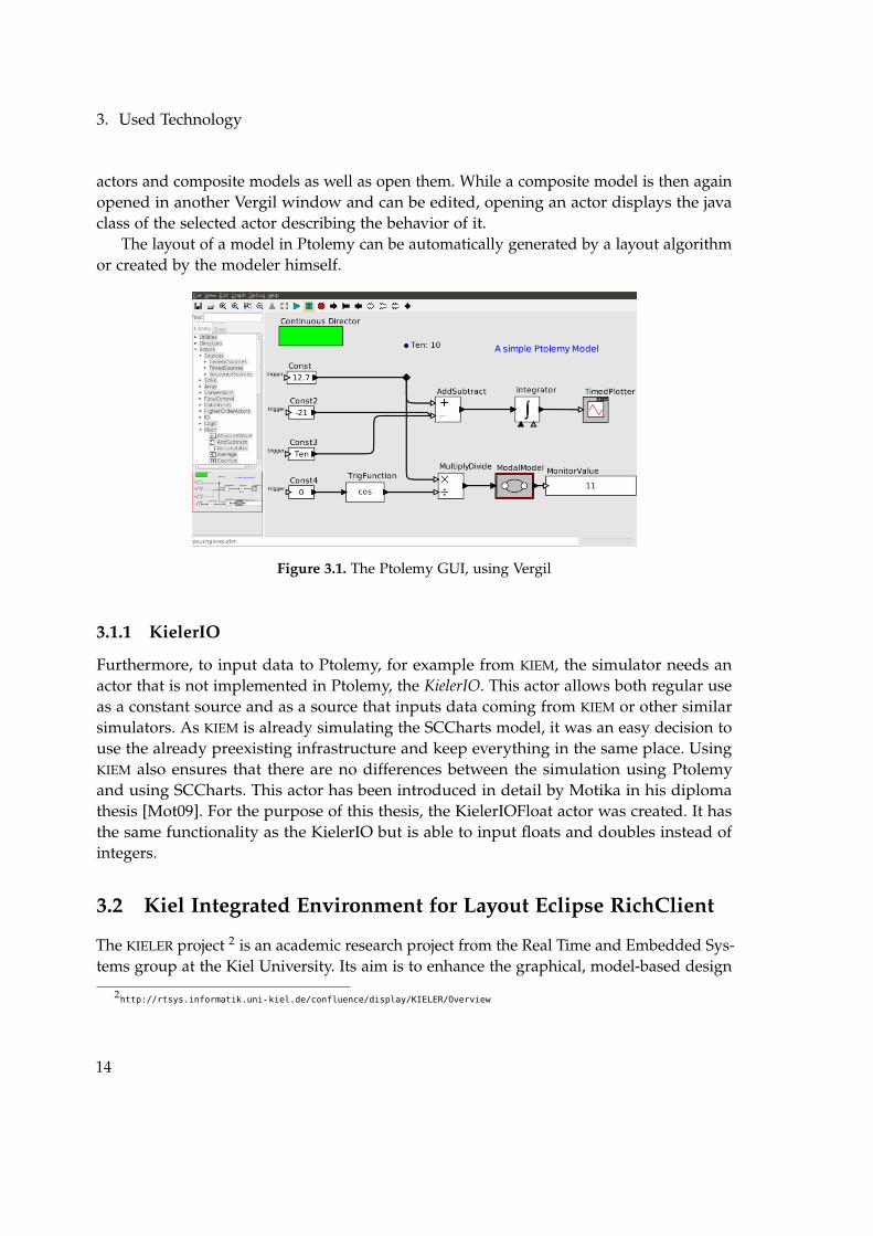
3. Used Technology

actors and composite models as well as open them. While a composite model is then againopened in another Vergil window and can be edited, opening an actor displays the javaclass of the selected actor describing the behavior of it.

The layout of a model in Ptolemy can be automatically generated by a layout algorithmor created by the modeler himself.

Figure 3.1. The Ptolemy GUI, using Vergil

3.1.1 KielerIO

Furthermore, to input data to Ptolemy, for example from KIEM, the simulator needs anactor that is not implemented in Ptolemy, the KielerIO. This actor allows both regular useas a constant source and as a source that inputs data coming from KIEM or other similarsimulators. As KIEM is already simulating the SCCharts model, it was an easy decision touse the already preexisting infrastructure and keep everything in the same place. UsingKIEM also ensures that there are no differences between the simulation using Ptolemyand using SCCharts. This actor has been introduced in detail by Motika in his diplomathesis [Mot09]. For the purpose of this thesis, the KielerIOFloat actor was created. It hasthe same functionality as the KielerIO but is able to input floats and doubles instead ofintegers.

3.2 Kiel Integrated Environment for Layout Eclipse RichClient

The KIELER project 2 is an academic research project from the Real Time and Embedded Sys-tems group at the Kiel University. Its aim is to enhance the graphical, model-based design

2http://rtsys.informatik.uni-kiel.de/confluence/display/KIELER/Overview

14

3.3. Java Simple Serial Connector

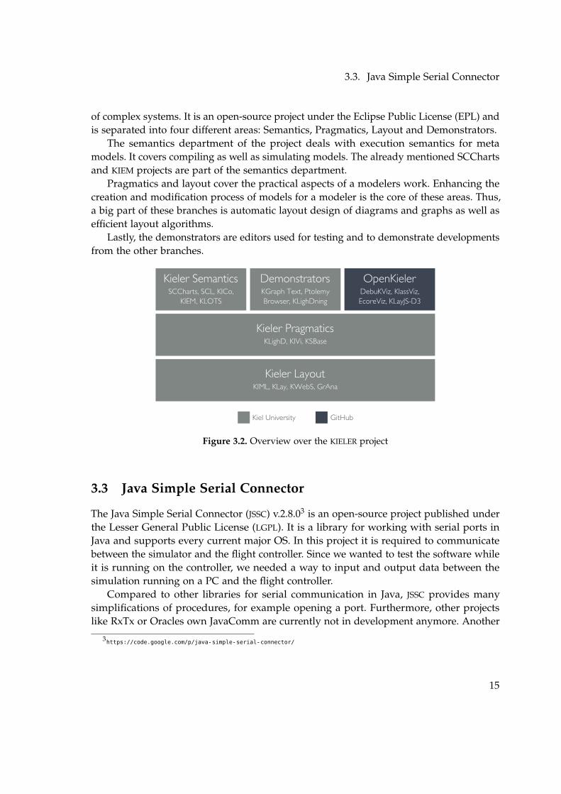
of complex systems. It is an open-source project under the Eclipse Public License (EPL) andis separated into four different areas: Semantics, Pragmatics, Layout and Demonstrators.

The semantics department of the project deals with execution semantics for metamodels. It covers compiling as well as simulating models. The already mentioned SCChartsand KIEM projects are part of the semantics department.

Pragmatics and layout cover the practical aspects of a modelers work. Enhancing thecreation and modification process of models for a modeler is the core of these areas. Thus,a big part of these branches is automatic layout design of diagrams and graphs as well asefficient layout algorithms.

Lastly, the demonstrators are editors used for testing and to demonstrate developmentsfrom the other branches.

Figure 3.2. Overview over the KIELER project

3.3 Java Simple Serial Connector

The Java Simple Serial Connector (JSSC) v.2.8.03 is an open-source project published underthe Lesser General Public License (LGPL). It is a library for working with serial ports inJava and supports every current major OS. In this project it is required to communicatebetween the simulator and the flight controller. Since we wanted to test the software whileit is running on the controller, we needed a way to input and output data between thesimulation running on a PC and the flight controller.

Compared to other libraries for serial communication in Java, JSSC provides manysimplifications of procedures, for example opening a port. Furthermore, other projectslike RxTx or Oracles own JavaComm are currently not in development anymore. Another

3https://code.google.com/p/java-simple-serial-connector/

15

3. Used Technology

reason for JSSC is that the current version of RxTx does not support Java 8 – at least withoutfurther modifications. JavaComm on the other hand is pretty much unusable and shouldnot be considered for serial communication in Java. It has not been properly updated inten years and official support has stopped. Therefore, even finding an official downloadlink proves to be difficult.

After completing the program, I have heard of a relatively new java serial library calledjSerialComm4. It is a platform independent library for serial communication with java. Itclaims to be very lightweight and efficient. A closer look into this library might be advisedfor future use.

3.4 Arduino Mega 2560

JSSC then communicates with software running on the quadcopter, more precisely onthe Arduino Mega 2560 board, for simplification in the following called Arduino, on thequadcopter. This flight controller is running on custom libraries and SCCharts generatedcode as the flight controller. The Mega 2560 is a microcontroller board based on theATmega2560 5 with 54 digital input/output pins, 16 analog inputs, four hardware serialports, a USB connection and more. The board can be supplied with power via the USBserial port as well as via battery over an input pin. Using the Arduino Software IDE 6,programs in C++ or the Arduino own Arduino language can be uploaded to the board.

We have chosen this board as we deemed it powerful enough while not being tooheavy, requiring too much voltage to run or not being able to output current at the desiredvoltage for our sensors. It also provides enough pins for our purposes. Too small boardsmight not have enough pins or might not run fast enough to calculate the flight propertiesin time. Furthermore, there was already a spare Arduino Mega in the office so the decisionwas easy to make.

Another alternative to an Arduino board was using a Raspberry Pi7 or a BeagleBone8

computer. These boards, as opposed to the Arduino boards, require an operating systemto run. Thus, they are not necessarily suitable as safety-critical systems as a safety-criticalsystem has to react as fast as possible to the environment and an operating systemmight interrupt critical computations with OS specific functionalities. This can lead tounpredictable behavior.

Andersen [And15] as well as Machaczek [Mac15] contain more information about theflight controller and the hard- and software of the quadcopter.

4http://fazecast.github.io/jSerialComm/5http://www.atmel.com/Images/Atmel-2549-8-bit-AVR-Microcontroller-ATmega640-1280-1281-2560-2561_datasheet.pdf6https://www.arduino.cc/en/Main/Software7https://www.raspberrypi.org/8http://beagleboard.org/

16

Chapter 4

Model and Simulation

To be able to compare Ptolemy and SCCharts, a model to simulate is required. Therefore,this chapter explains the physical and mathematical properties of the quadcopter. Sec-tion 4.1 contains all the equations and their backgrounds, explaining the model in detail. Italso explains the rotations required to describe the model accurately and afterwards theproperties pertaining to the acceleration as well as to the angles. The section concludeswith information about the physical properties of the simulated quadcopter. Followingthat, Section 4.2 discusses how to integrate the simulation into the setup of the simulationusing KIEM.

4.1 Mathematical Model

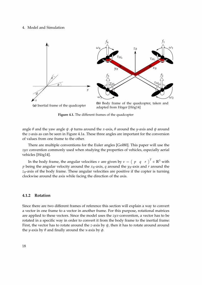
Before going into detail, this section explains a few necessities for the model. As shownin Figure 4.1, the quadcopter has to be viewed in two different frames: First, the inertialframe, seen on the left, is the frame of the room. It is fixed and cannot change. Second,the body frame, as seen on the right, is the frame of the copter. Its axes, the body axesxB, yB and zB, are fixed to the arms and body of the quadcopter and its point of origin isthe center of mass, so it moves with the copter at all times. These frames of reference arenecessary, as the simulation will send data calculated from both frames to the Arduino,which Section 4.2 describes in more detail. The inertial frame is important for the locationof the vehicle and thus for the distances to the walls and the body frame is needed forgyroscopic values like the angular velocities or the linear acceleration of the quadcopter.Furthermore, to compute these values, calculations in both frames are required as will beevident from the descriptions in this chapter.

In the sections pertaining to the angles and angular velocities, Newton-Euler equa-tions [Hah02] describe the behavior of the copter. Since the copter is assumed to be a rigidbody, these equations can be used to describe the dynamics of the quadcopter [Luu11].

4.1.1 Fundamental of the model

The absolute linear position of the quadcopter is defined in the inertial frame of thequadcopter by ξ =

(x y z

) T P R3 and the Euler angles describing the rotation of

the quadcopter are defined by η =(

φ θ ψ)T

P R3 with the roll angle φ, the pitch

17

4. Model and Simulation

φ

θ

ψ

z

x

y

(a) Inertial frame of the quadcopter

xByB

zB

f1

f2f3

f4

ω4

τM1τM4

τM3τM2

ω2ω3

ω1

(b) Body frame of the quadcopter, taken andadapted from Höger [Hög14]

Figure 4.1. The different frames of the quadcopter

angle θ and the yaw angle ψ. φ turns around the x-axis, θ around the y-axis and ψ aroundthe z-axis as can be seen in Figure 4.1a. These three angles are important for the conversionof values from one frame to the other.

There are multiple conventions for the Euler angles [Gol80]. This paper will use thezyx convention commonly used when studying the properties of vehicles, especially aerialvehicles [Hög14].

In the body frame, the angular velocities ν are given by ν =(

p q r)TP R3 with

p being the angular velocity around the xB-axis, q around the yB-axis and r around thezB-axis of the body frame. These angular velocities are positive if the copter is turningclockwise around the axis while facing the direction of the axis.

4.1.2 Rotation

Since there are two different frames of reference this section will explain a way to converta vector in one frame to a vector in another frame. For this purpose, rotational matricesare applied to these vectors. Since the model uses the zyx-convention, a vector has to berotated in a specific way in order to convert it from the body frame to the inertial frame:First, the vector has to rotate around the z-axis by ψ, then it has to rotate around aroundthe y-axis by θ and finally around the x-axis by φ.

18

4.1. Mathematical Model

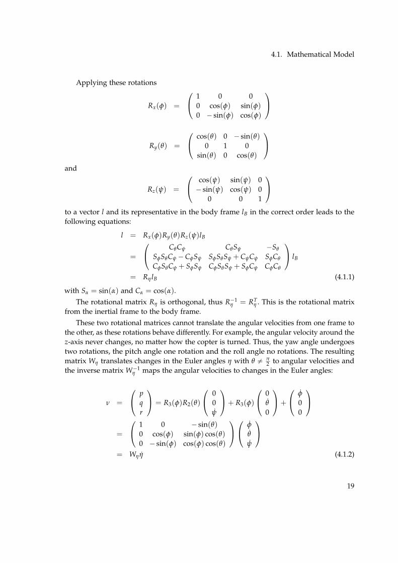
Applying these rotations

Rx(φ) =

1 0 00 cos(φ) sin(φ)0 ´ sin(φ) cos(φ)

Ry(θ) =

cos(θ) 0 ´ sin(θ)0 1 0

sin(θ) 0 cos(θ)

and

Rz(ψ) =

cos(ψ) sin(ψ) 0´ sin(ψ) cos(ψ) 0

0 0 1

to a vector l and its representative in the body frame lB in the correct order leads to thefollowing equations:

l = Rx(φ)Ry(θ)Rz(ψ)lB

=

CθCψ CθSψ ´Sθ

SφSθCψ ´ CφSψ SφSθSψ + CψCψ SφCθ

CφSθCψ + SφSψ CφSθSψ + SφCψ CφCθ

lB

= Rη lB (4.1.1)

with Sα = sin(α) and Cα = cos(α).

The rotational matrix Rη is orthogonal, thus R´1η = RT

η . This is the rotational matrixfrom the inertial frame to the body frame.

These two rotational matrices cannot translate the angular velocities from one frame tothe other, as these rotations behave differently. For example, the angular velocity around thez-axis never changes, no matter how the copter is turned. Thus, the yaw angle undergoestwo rotations, the pitch angle one rotation and the roll angle no rotations. The resultingmatrix Wη translates changes in the Euler angles η with θ ‰ π

2 to angular velocities andthe inverse matrix W´1

η maps the angular velocities to changes in the Euler angles:

ν =

pqr

= R3(φ)R2(θ)

00ψ

+ R3(φ)

0θ

0

+

φ

00

=

1 0 ´ sin(θ)0 cos(φ) sin(φ) cos(θ)0 ´ sin(φ) cos(φ) cos(θ)

φ

θ

ψ

= Wη η (4.1.2)

19

4. Model and Simulation

zB

xB

yB

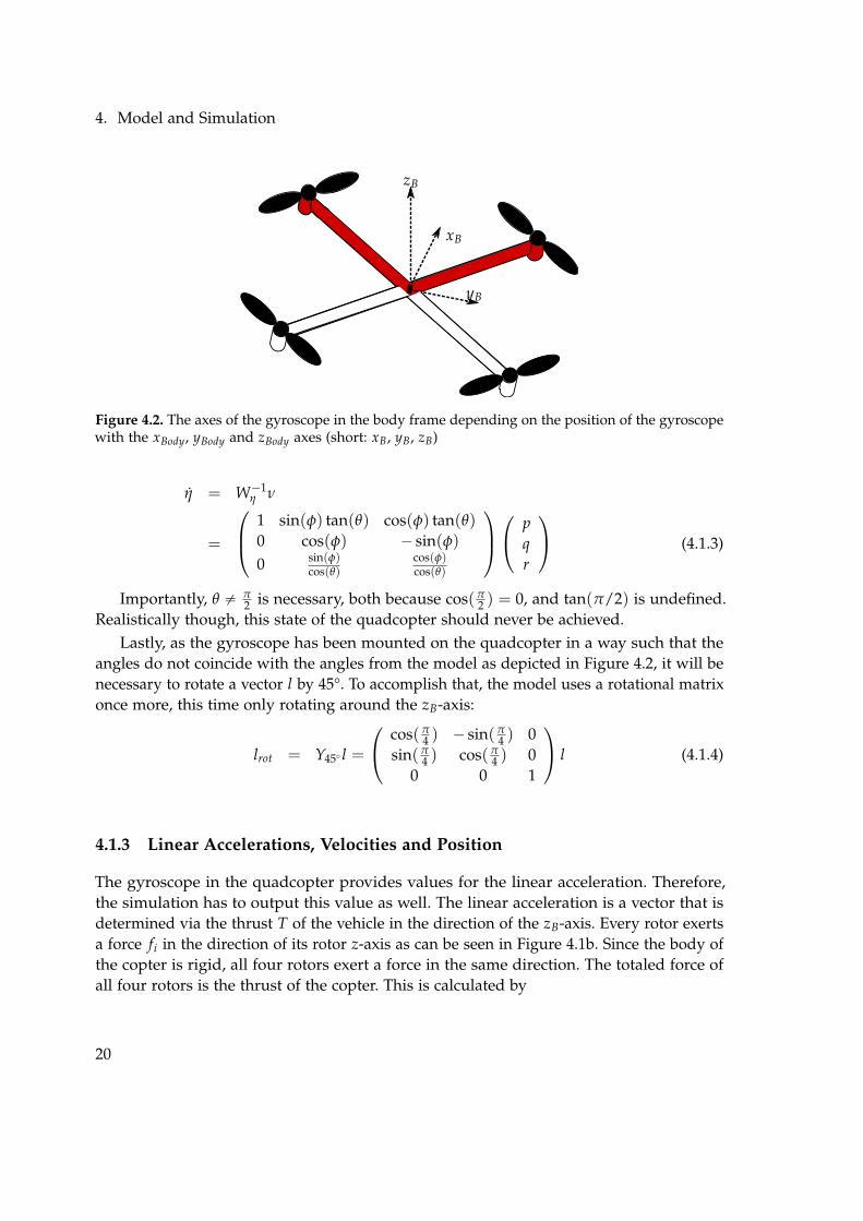
Figure 4.2. The axes of the gyroscope in the body frame depending on the position of the gyroscopewith the xBody, yBody and zBody axes (short: xB, yB, zB)

η = W´1η ν

=

1 sin(φ) tan(θ) cos(φ) tan(θ)0 cos(φ) ´ sin(φ)0 sin(φ)

cos(θ)cos(φ)cos(θ)

p

qr

(4.1.3)

Importantly, θ ‰ π2 is necessary, both because cos(π

2 ) = 0, and tan(π/2) is undefined.Realistically though, this state of the quadcopter should never be achieved.

Lastly, as the gyroscope has been mounted on the quadcopter in a way such that theangles do not coincide with the angles from the model as depicted in Figure 4.2, it will benecessary to rotate a vector l by 45°. To accomplish that, the model uses a rotational matrixonce more, this time only rotating around the zB-axis:

lrot = Y450 l =

cos(π4 ) ´ sin(π

4 ) 0sin(π

4 ) cos(π4 ) 0

0 0 1

l (4.1.4)

4.1.3 Linear Accelerations, Velocities and Position

The gyroscope in the quadcopter provides values for the linear acceleration. Therefore,the simulation has to output this value as well. The linear acceleration is a vector that isdetermined via the thrust T of the vehicle in the direction of the zB-axis. Every rotor exertsa force fi in the direction of its rotor z-axis as can be seen in Figure 4.1b. Since the body ofthe copter is rigid, all four rotors exert a force in the same direction. The totaled force ofall four rotors is the thrust of the copter. This is calculated by

20

4.1. Mathematical Model

fi = lω2i (4.1.5)

T =4

∑i=1

fi = l4

∑i=1

ω2i (4.1.6)

with l being the lift constant1 and ωi being the angular velocity of the rotor corresponding tothe motor i. The calculated thrust exerts constantly along the z-axis of the quadcopter andis therefore in the body frame. By applying the rotational matrix Rη from Equation 4.1.1to the vectorized thrust, we can translate this force into the inertial frame. Additionally,gravity exerts on the quadcopter. Therefore it has to be subtracted from the accelerationprovided by the thrust.

a =

xyz

=

00´g

+

00Tm

Rη

=

00´g

+Tm

cos(φ) sin(θ) cos(ψ) + sin(φ) sin(ψ)cos(φ) sin(θ) sin(ψ)´ sin(φ) cos(ψ)

cos(φ) cos(θ)

(4.1.7)

This acceleration though does not yet factor in aerodynamic effects. Thus, the followingequation describes these effects with the drag force coefficients Ax, Ay and Az and thevelocity v slowing the acceleration down.

xyz

= a´1m

Ax 0 00 Ay 00 0 Az

v (4.1.8)

The velocity v has to be known to calculate the acceleration, which in turn has to beknown to calculate the velocity. Thus, a loop-back is required.

Now that the linear acceleration is known, this value is integrated over time to calculatethe velocity v and integrated once more to calculate the current position ξ of the quadcopter.

4.1.4 Angular Velocities and Angles

To actually apply the rotational matrices mentioned above, the Euler angles η have to becomputed. Thus, it is necessary to calculate the torques τφ, τθ and τψ in the direction of thecorresponding body frame axes:

1More about the lift and drag constants can be read here:http://mragheb.com/NPRE475WindPowerSystems/AeorodynamicsofRotorBlades.pdf

21

4. Model and Simulation

τ =

τφ

τθ

τψ

=

drl(´ω22 + ω2

4)

drl(´ω21 + ω2

3)

∑4i=1 τMi

(4.1.9)

with dr being the distance between the rotor middle and the center of mass of the quad-copter, l being the lift constant1 mentioned before and

τMi = bω2i + IMωi (4.1.10)

where b is the drag constant1 of the rotors and IM is the inertia moment of the rotors. Sincethe rotor acceleration ωi as well as the inertia moment IM is very small, it is omitted.

This implies that movement in the roll direction can be increased by increasing thevelocity of the fourth rotor and/or decreasing the velocity of the second rotor. Likewise,pitch direction movement can be increased by increasing the velocity of the third rotorand/or decreasing the velocity of the first rotor. Turning around the zB-axis can be achievedby increasing opposite rotors and decreasing the other two rotors. These movements canobviously be combined to create a smooth turning of the copter if wanted.

In the body frame, the angular acceleration Iν together with the centripetal forcesν ˆ (Iν) and the gyroscopic forces Γ equal the torque τ. Thus, with a little bit ofreorganizing, the following equation can be formulated:

Iν + νˆ (Iν) + Γ = τ (4.1.11)

ν = I´1

´ p

qr

ˆ Ixx p

IyyqIzzr

´ Ir

pqr

ˆ 0

01

ωτ + τ

=

1

Ixx1

Iyy1

Izz

(Iyy ´ Izz)qr

(Izz ´ Ixx)pr(Ixx ´ Iyy)pq

´ Irωτ

q´p0

+

τφ

τθ

τψ

(4.1.12)

with ωτ = ω1 ´ω2 + ω3 ´ω4.

The derivative of the angular accelerations ν from the equation above can now calculatethe angular velocities ν in the body frame by integrating them over time. These values arean output value of the gyroscope.

Furthermore, the angular velocities ν, translated to the inertial frame with the help ofthe rotation matrix W´1

η from Equation 4.1.2, when integrated, result in the current anglesη.

22

4.1. Mathematical Model

wle f t

dle f t

ψwle f t + x

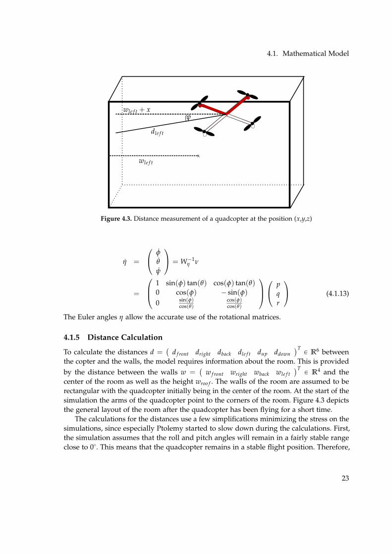
Figure 4.3. Distance measurement of a quadcopter at the position (x,y,z)

η =

φ

θ

ψ

= W´1η ν

=

1 sin(φ) tan(θ) cos(φ) tan(θ)0 cos(φ) ´ sin(φ)0 sin(φ)

cos(θ)cos(φ)cos(θ)

p

qr

(4.1.13)

The Euler angles η allow the accurate use of the rotational matrices.

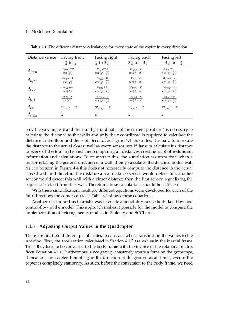
4.1.5 Distance Calculation

To calculate the distances d =(

d f ront dright dback dle f t dup ddown)TP R6 between

the copter and the walls, the model requires information about the room. This is providedby the distance between the walls w =

(w f ront wright wback wle f t

)TP R4 and the

center of the room as well as the height wroo f . The walls of the room are assumed to berectangular with the quadcopter initially being in the center of the room. At the start of thesimulation the arms of the quadcopter point to the corners of the room. Figure 4.3 depictsthe general layout of the room after the quadcopter has been flying for a short time.

The calculations for the distances use a few simplifications minimizing the stress on thesimulations, since especially Ptolemy started to slow down during the calculations. First,the simulation assumes that the roll and pitch angles will remain in a fairly stable rangeclose to 00. This means that the quadcopter remains in a stable flight position. Therefore,

23

4. Model and Simulation

Table 4.1. The different distance calculations for every state of the copter in every direction

Distance sensor Facing front´π

4 to π4

Facing rightπ4 to 3 π

4

Facing back3 π

4 to ´3 π4

Facing left´3 π

4 to ´π4

d f rontw f ront´ycos(ψ)

wright´xcos(ψ´ π

2 )wback+y

cos(ψ´π)

wle f t+xcos(ψ+ π

2 )

drightwright´xcos(ψ)

wback+ycos(ψ´ π

2 )

wle f t+xcos(ψ´π)

w f ront´ycos(ψ+ π

2 )

dbackwback+ycos(ψ)

wle f t+xcos(ψ´ π

2 )

w f ront´ycos(ψ´π)

wright´xcos(ψ+ π

2 )

dle f twle f t+xcos(ψ)

w f ront´ycos(ψ´ π

2 )

wright´xcos(ψ´π)

wback+ycos(ψ+ π

2 )

dup wroo f ´ z wroo f ´ z wroo f ´ z wroo f ´ z

ddown z z z z

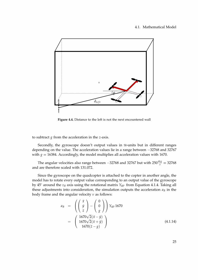
only the yaw angle ψ and the x and y coordinates of the current position ξ is necessary tocalculate the distance to the walls and only the z coordinate is required to calculate thedistance to the floor and the roof. Second, as Figure 4.4 illustrates, it is hard to measurethe distance to the actual closest wall as every sensor would have to calculate his distanceto every of the four walls and then comparing all distances creating a lot of redundantinformation and calculations. To counteract this, the simulation assumes that, when asensor is facing the general direction of a wall, it only calculates the distance to this wall.As can be seen in Figure 4.4 this does not necessarily compute the distance to the actualclosest wall and therefore the distance a real distance sensor would detect. Yet, anothersensor would detect this wall with a closer distance then the first sensor, signalizing thecopter to back off from this wall. Therefore, these calculations should be sufficient.

With these simplifications multiple different equations were developed for each of thefour directions the copter can face. Table 4.1 shows these equations.

Another reason for this heuristic was to create a possibility to use both data-flow andcontrol-flow in the model. This approach makes it possible for the model to compare theimplementation of heterogeneous models in Ptolemy and SCCharts.

4.1.6 Adjusting Output Values to the Quadcopter

There are multiple different peculiarities to consider when transmitting the values to theArduino. First, the acceleration calculated in Section 4.1.3 are values in the inertial frame.Thus, they have to be converted to the body frame with the inverse of the rotational matrixfrom Equation 4.1.1. Furthermore, since gravity constantly exerts a force on the gyroscope,it measures an acceleration of ´g in the direction of the ground at all times, even if thecopter is completely stationary. As such, before the conversion to the body frame, we need

24

4.1. Mathematical Model

dle f t

ψ

Figure 4.4. Distance to the left is not the next encountered wall

to subtract g from the acceleration in the z-axis.

Secondly, the gyroscope doesn’t output values in SI-units but in different rangesdepending on the value. The acceleration values lie in a range between ´32768 and 32767with g ” 16384. Accordingly, the model multiplies all acceleration values with 1670.

The angular velocities also range between ´32768 and 32767 but with 250 degs ” 32768

and are therefore scaled with 131.072.

Since the gyroscope on the quadcopter is attached to the copter in another angle, themodel has to rotate every output value corresponding to an output value of the gyroscopeby 450 around the zB axis using the rotational matrix Y450 from Equation 4.1.4. Taking allthese adjustments into consideration, the simulation outputs the acceleration aB in thebody frame and the angular velocity ν as follows:

aB =

xyz

´ 0

0g

Y4501670

=

1670√

2(x´ y)1670

√2(x + y)

1670(z´ g)

(4.1.14)

25

4. Model and Simulation

Table 4.2. The different constants of the quadcopter and their respective units

Parameter Value Unit

g 9.81 m/s2

m 0.468 kgdr 0.225 mAx 0.25 kg/sAy 0.25 kg/sAz 0.25 kg/s

Parameter Value Unit

l 2.980 ˚ 10´6 –b 1.140 ˚ 10´7 –IM 3.357 ˚ 10´5 kg m2

Ixx 4.856 ˚ 10´3 kg m2

Iyy 4.856 ˚ 10´3 kg m2

Izz 8.801 ˚ 10´3 kg m2

ν =

pqr

Y450131.072 =

131.072√

2(q´ p)131.072

√2(q + p)

131.072(r´ g)

(4.1.15)

Lastly, the ultrasonic sensors of the quadcopter only output values in cm. Therefore thedistance values are multiplied by 100 to accommodate this.

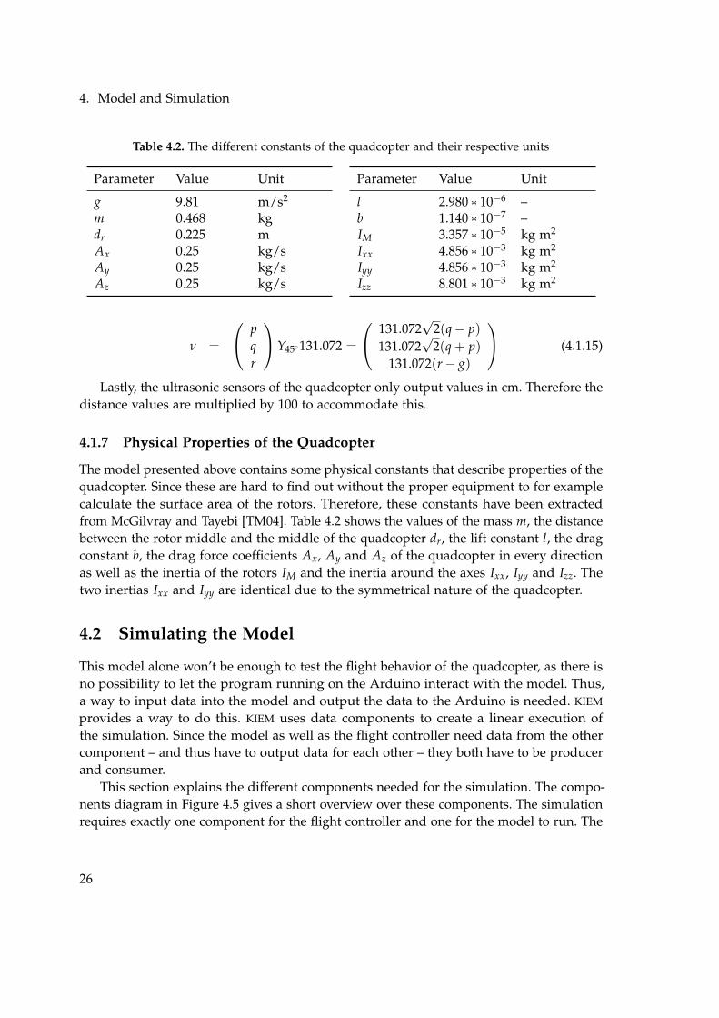
4.1.7 Physical Properties of the Quadcopter

The model presented above contains some physical constants that describe properties of thequadcopter. Since these are hard to find out without the proper equipment to for examplecalculate the surface area of the rotors. Therefore, these constants have been extractedfrom McGilvray and Tayebi [TM04]. Table 4.2 shows the values of the mass m, the distancebetween the rotor middle and the middle of the quadcopter dr, the lift constant l, the dragconstant b, the drag force coefficients Ax, Ay and Az of the quadcopter in every directionas well as the inertia of the rotors IM and the inertia around the axes Ixx, Iyy and Izz. Thetwo inertias Ixx and Iyy are identical due to the symmetrical nature of the quadcopter.

4.2 Simulating the Model

This model alone won’t be enough to test the flight behavior of the quadcopter, as there isno possibility to let the program running on the Arduino interact with the model. Thus,a way to input data into the model and output the data to the Arduino is needed. KIEM

provides a way to do this. KIEM uses data components to create a linear execution ofthe simulation. Since the model as well as the flight controller need data from the othercomponent – and thus have to output data for each other – they both have to be producerand consumer.

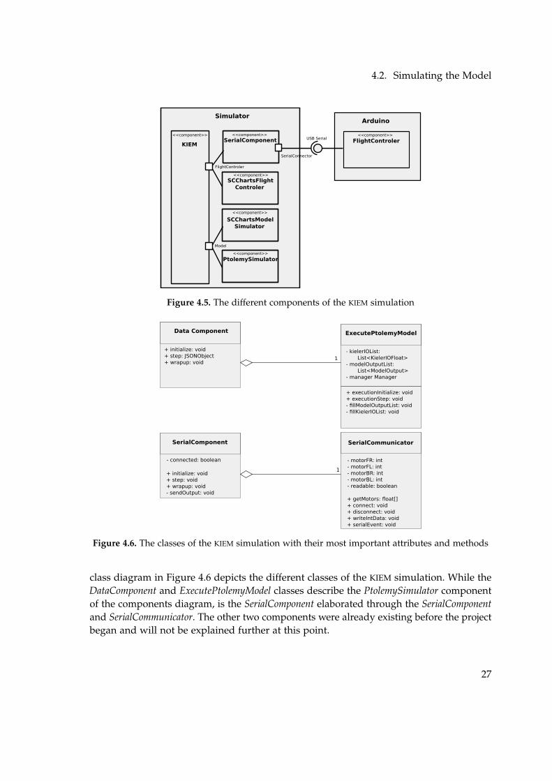
This section explains the different components needed for the simulation. The compo-nents diagram in Figure 4.5 gives a short overview over these components. The simulationrequires exactly one component for the flight controller and one for the model to run. The

26

4.2. Simulating the Model

Simulator

KIEMSerialComponent

SCChartsFlight Controler

SCChartsModel Simulator

PtolemySimulator

Arduino

FlightControler<<component>> <<component>>

<<component>>

<<component>>

<<component>>

<<component>>USB Serial

SerialConnector

FlightControler

Model

Figure 4.5. The different components of the KIEM simulation

Data Component

+ initialize: void+ step: JSONObject+ wrapup: void

SerialComponent

- connected: boolean

+ initialize: void+ step: void+ wrapup: void- sendOutput: void

SerialCommunicator

- motorFR: int- motorFL: int- motorBR: int- motorBL: int- readable: boolean

+ getMotors: float[]+ connect: void+ disconnect: void+ writeIntData: void+ serialEvent: void

ExecutePtolemyModel

- kielerIOList: List<KielerIOFloat>- modelOutputList: List<ModelOutput>- manager Manager

+ executionInitialize: void+ executionStep: void- fillModelOutputList: void- fillKielerIOList: void

1

1

Figure 4.6. The classes of the KIEM simulation with their most important attributes and methods

class diagram in Figure 4.6 depicts the different classes of the KIEM simulation. While theDataComponent and ExecutePtolemyModel classes describe the PtolemySimulator componentof the components diagram, is the SerialComponent elaborated through the SerialComponentand SerialCommunicator. The other two components were already existing before the projectbegan and will not be explained further at this point.

27

4. Model and Simulation

4.2.1 Simulating the Flight Controller

To simulate the flight controller the user has two choices: He can either run the programon the Arduino to test the compatibility of the software and hardware or run it on thesimulating PC. If the user wants to run the execution completely on the simulating PC,he can use the SCChart of the flight controller. KIEM is able to simulate any SCChartthat is compilable. Running the flight controller on the Arduino however requires aserial connection to the Arduino that is realized in KIEM using the implemented ArduinoCommunication data component. This data component uses the SerialCommunicator javaclass which in turn uses JSSC to establish a serial connection between the simulation andthe Arduino.

Communication Protocol

The communication follows a simple protocol. First, the Arduino sends the four motorvalues together with an identifying character – a number assigned to the motor in thebeginning of the project that corresponds to the pin it was connected to on the Arduino. Thesimulation simply waits for all four motors to be transmitted. Afterwards, the simulationsends every important output of the model to the Arduino. Similarly, the simulation sendsan identifying character with each output. Since the data being transmitted to the Arduinois in integers and not in bytes and the serial communication can only transmit single bytesat a time, the serial communication class cuts the integer into four bytes and sends theseone by one over to the Arduino which in turn converts these bytes back to an integer.Closing the communication is a delimiter byte from the simulation signaling the Arduinothat it can now continue with his calculations. On the other side, the simulation can simplycontinue with its computations as it does not need any more input data from the flightcontroller.

Alternatives to the Arduino and SCCharts

The Arduino itself is not necessary for the simulation. Both the code of the flight controlleras well as the model should theoretically be testable by running everything via KIEM. Theprerequisite for this is that there exists a way to simulate the flight controller in KIEM. Sincethe code on the Arduino that controls the flight behavior has been written with SCCharts,KIEM can easily simulate the flight controller.

If the code is not written in SCCharts, then a new data component would have to bedeveloped. As there was code written for the flight controller in C and C++ as well forcomparison purposes, a new component would have to be written to test this. This wasnot done in the scope of this paper due to time constraints and since the code was alreadytested and deemed working as of the completion of the simulation.

28

4.2. Simulating the Model

For further information on creating data components in KIEM, reading the diplomathesis of Motika [Mot09] is advised.

4.2.2 Simulating the Model in KIEM

To simulate Ptolemy in KIEM the data component Simple Ptolemy Simulator, which is createdby the DataComponent class, is used. It is a component developed by Motika [Mot09] andcleaned up for this thesis that loads a Ptolemy XML file for the simulation. The Ptolemymodel is then executed stepwise with every step of the KIEM execution. KIEM provides themodel with input data of the motors and extracts the outputs of the simulation via thecommunication bus.

Similarly, the SCCharts model can be executed using the SCCharts / SCG Simulator (C)data component. This data component was already implemented prior to this thesis andcomes with two other data components accompanying it. The Synchronous Signal Resetterand the Synchronous Signal View. While the former resets every synchronous signal at thebeginning of each tick to ensure that each signal is present if and only if it is set to presentin this tick, the latter creates a view showing the value of every signal at every tick. Both ofthese are rather unimportant for this project and could be omitted. Similar to the Ptolemymodel, the SCChart is executed stepwise by KIEM and exchanges inputs and outputs withthe communication bus of the simulation.

29

Chapter 5

Realization

After establishing the physical properties in the previous chapter, the next section coversthe realization of these models. It first explains the realization with the tool Ptolemy aswell as with SCCharts. Afterwards, this chapter covers the implementations required tosimulate the model using KIEM and concludes with the realization of the data exchangebetween the Arduino and the simulation.

5.1 Realization with Ptolemy

The properties from Chapter 4 were subsequently modeled in Ptolemy using a continu-ous time director as explained in the book System Design, Modeling and Simulation usingPtolemy II [Pto14].

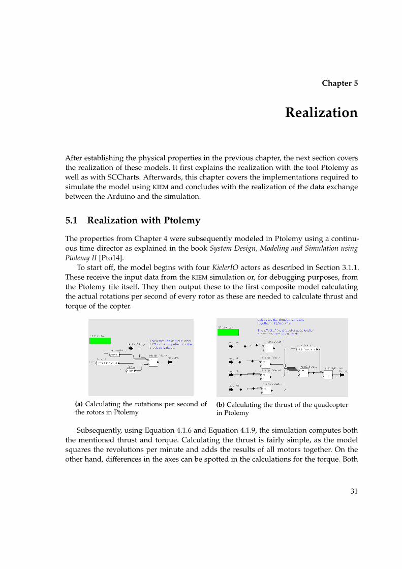
To start off, the model begins with four KielerIO actors as described in Section 3.1.1.These receive the input data from the KIEM simulation or, for debugging purposes, fromthe Ptolemy file itself. They then output these to the first composite model calculatingthe actual rotations per second of every rotor as these are needed to calculate thrust andtorque of the copter.

(a) Calculating the rotations per second ofthe rotors in Ptolemy

(b) Calculating the thrust of the quadcopterin Ptolemy

Subsequently, using Equation 4.1.6 and Equation 4.1.9, the simulation computes boththe mentioned thrust and torque. Calculating the thrust is fairly simple, as the modelsquares the revolutions per minute and adds the results of all motors together. On theother hand, differences in the axes can be spotted in the calculations for the torque. Both

31

5. Realization

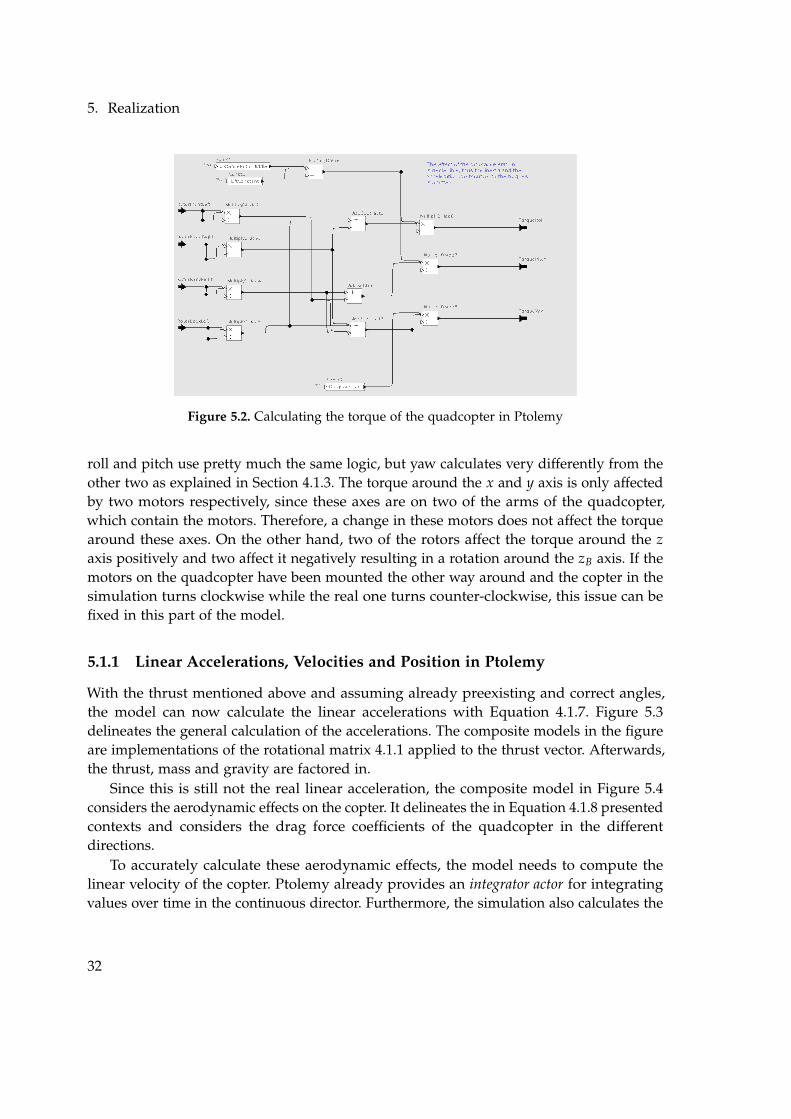
Figure 5.2. Calculating the torque of the quadcopter in Ptolemy

roll and pitch use pretty much the same logic, but yaw calculates very differently from theother two as explained in Section 4.1.3. The torque around the x and y axis is only affectedby two motors respectively, since these axes are on two of the arms of the quadcopter,which contain the motors. Therefore, a change in these motors does not affect the torquearound these axes. On the other hand, two of the rotors affect the torque around the zaxis positively and two affect it negatively resulting in a rotation around the zB axis. If themotors on the quadcopter have been mounted the other way around and the copter in thesimulation turns clockwise while the real one turns counter-clockwise, this issue can befixed in this part of the model.

5.1.1 Linear Accelerations, Velocities and Position in Ptolemy

With the thrust mentioned above and assuming already preexisting and correct angles,the model can now calculate the linear accelerations with Equation 4.1.7. Figure 5.3delineates the general calculation of the accelerations. The composite models in the figureare implementations of the rotational matrix 4.1.1 applied to the thrust vector. Afterwards,the thrust, mass and gravity are factored in.

Since this is still not the real linear acceleration, the composite model in Figure 5.4considers the aerodynamic effects on the copter. It delineates the in Equation 4.1.8 presentedcontexts and considers the drag force coefficients of the quadcopter in the differentdirections.

To accurately calculate these aerodynamic effects, the model needs to compute thelinear velocity of the copter. Ptolemy already provides an integrator actor for integratingvalues over time in the continuous director. Furthermore, the simulation also calculates the

32

5.1. Realization with Ptolemy

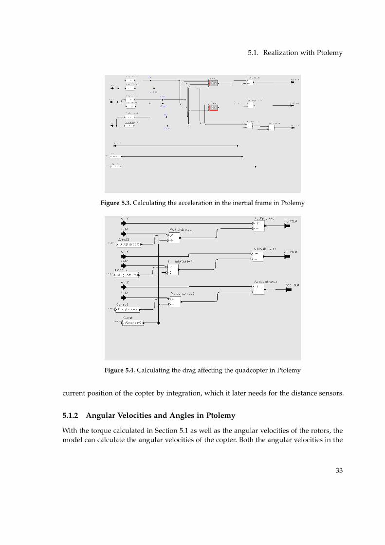
Figure 5.3. Calculating the acceleration in the inertial frame in Ptolemy

Figure 5.4. Calculating the drag affecting the quadcopter in Ptolemy

current position of the copter by integration, which it later needs for the distance sensors.

5.1.2 Angular Velocities and Angles in Ptolemy

With the torque calculated in Section 5.1 as well as the angular velocities of the rotors, themodel can calculate the angular velocities of the copter. Both the angular velocities in the

33

5. Realization

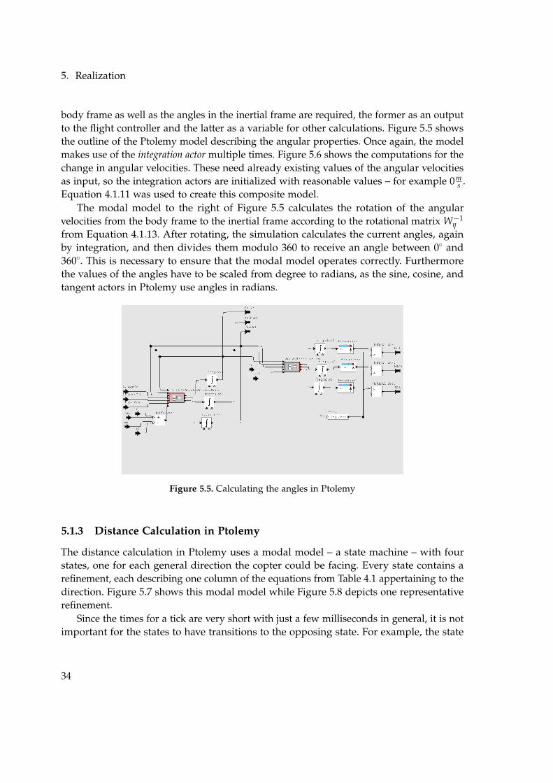
body frame as well as the angles in the inertial frame are required, the former as an outputto the flight controller and the latter as a variable for other calculations. Figure 5.5 showsthe outline of the Ptolemy model describing the angular properties. Once again, the modelmakes use of the integration actor multiple times. Figure 5.6 shows the computations for thechange in angular velocities. These need already existing values of the angular velocitiesas input, so the integration actors are initialized with reasonable values – for example 0 m

s .Equation 4.1.11 was used to create this composite model.

The modal model to the right of Figure 5.5 calculates the rotation of the angularvelocities from the body frame to the inertial frame according to the rotational matrix W´1

η

from Equation 4.1.13. After rotating, the simulation calculates the current angles, againby integration, and then divides them modulo 360 to receive an angle between 00 and3600. This is necessary to ensure that the modal model operates correctly. Furthermorethe values of the angles have to be scaled from degree to radians, as the sine, cosine, andtangent actors in Ptolemy use angles in radians.

Figure 5.5. Calculating the angles in Ptolemy

5.1.3 Distance Calculation in Ptolemy

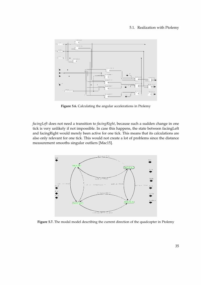
The distance calculation in Ptolemy uses a modal model – a state machine – with fourstates, one for each general direction the copter could be facing. Every state contains arefinement, each describing one column of the equations from Table 4.1 appertaining to thedirection. Figure 5.7 shows this modal model while Figure 5.8 depicts one representativerefinement.

Since the times for a tick are very short with just a few milliseconds in general, it is notimportant for the states to have transitions to the opposing state. For example, the state

34

5.1. Realization with Ptolemy

Figure 5.6. Calculating the angular accelerations in Ptolemy

facingLeft does not need a transition to facingRight, because such a sudden change in onetick is very unlikely if not impossible. In case this happens, the state between facingLeftand facingRight would merely been active for one tick. This means that its calculations arealso only relevant for one tick. This would not create a lot of problems since the distancemeasurement smooths singular outliers [Mac15].

Figure 5.7. The modal model describing the current direction of the quadcopter in Ptolemy

35

5. Realization

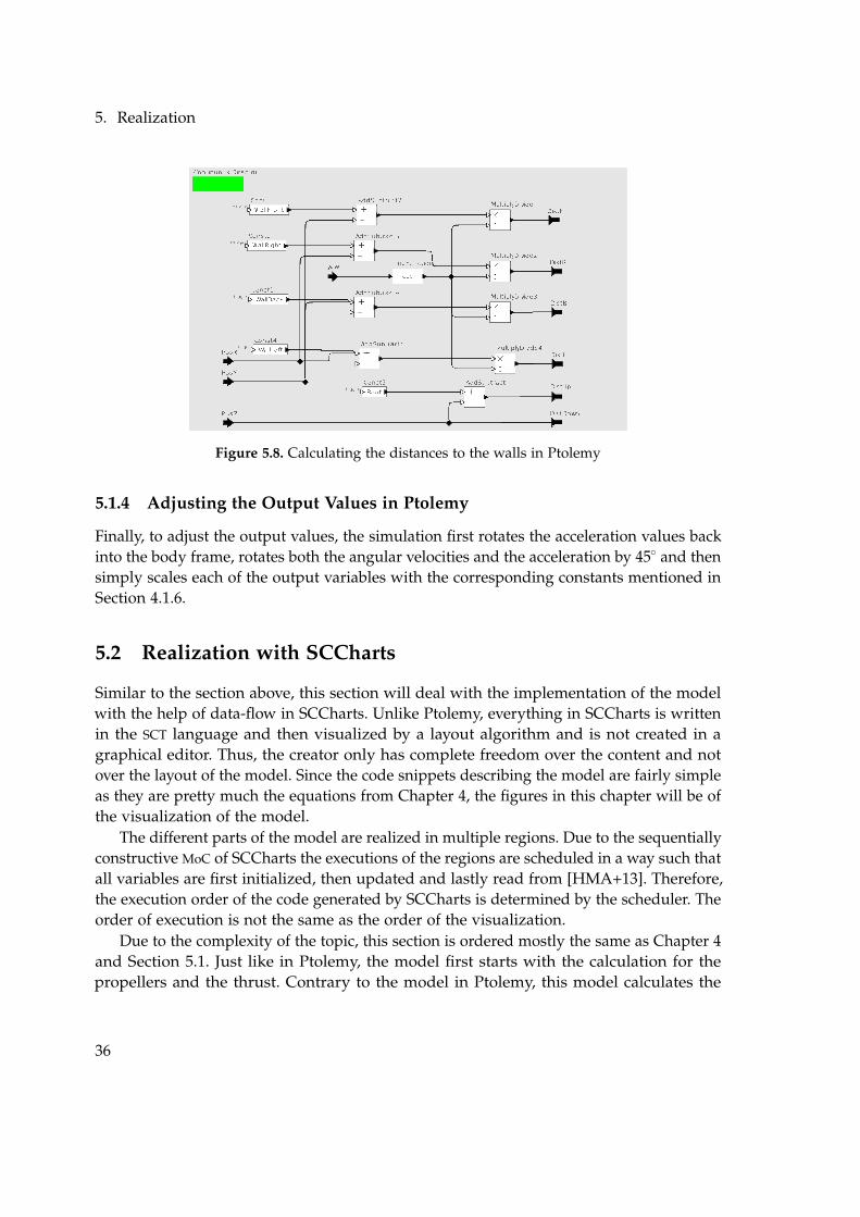
Figure 5.8. Calculating the distances to the walls in Ptolemy

5.1.4 Adjusting the Output Values in Ptolemy

Finally, to adjust the output values, the simulation first rotates the acceleration values backinto the body frame, rotates both the angular velocities and the acceleration by 450 and thensimply scales each of the output variables with the corresponding constants mentioned inSection 4.1.6.

5.2 Realization with SCCharts

Similar to the section above, this section will deal with the implementation of the modelwith the help of data-flow in SCCharts. Unlike Ptolemy, everything in SCCharts is writtenin the SCT language and then visualized by a layout algorithm and is not created in agraphical editor. Thus, the creator only has complete freedom over the content and notover the layout of the model. Since the code snippets describing the model are fairly simpleas they are pretty much the equations from Chapter 4, the figures in this chapter will be ofthe visualization of the model.

The different parts of the model are realized in multiple regions. Due to the sequentiallyconstructive MoC of SCCharts the executions of the regions are scheduled in a way such thatall variables are first initialized, then updated and lastly read from [HMA+13]. Therefore,the execution order of the code generated by SCCharts is determined by the scheduler. Theorder of execution is not the same as the order of the visualization.

Due to the complexity of the topic, this section is ordered mostly the same as Chapter 4and Section 5.1. Just like in Ptolemy, the model first starts with the calculation for thepropellers and the thrust. Contrary to the model in Ptolemy, this model calculates the

36

5.2. Realization with SCCharts

motorRPMpV

2

*

pi

60

/

*

helperRPM

FrontRight*

propFRRPMFrontLeft

*

propFLRPM

BackRight *

propBRRPM

BackLeft

*

propBLRPM

*

pFRRPMSquare

*pFLRPMSquare

*pBRRPMSquare

*pBLRPMSquare

+ +

+

liftConstant*

thrust

Figure 5.9. Calculating the thrust in SCCharts

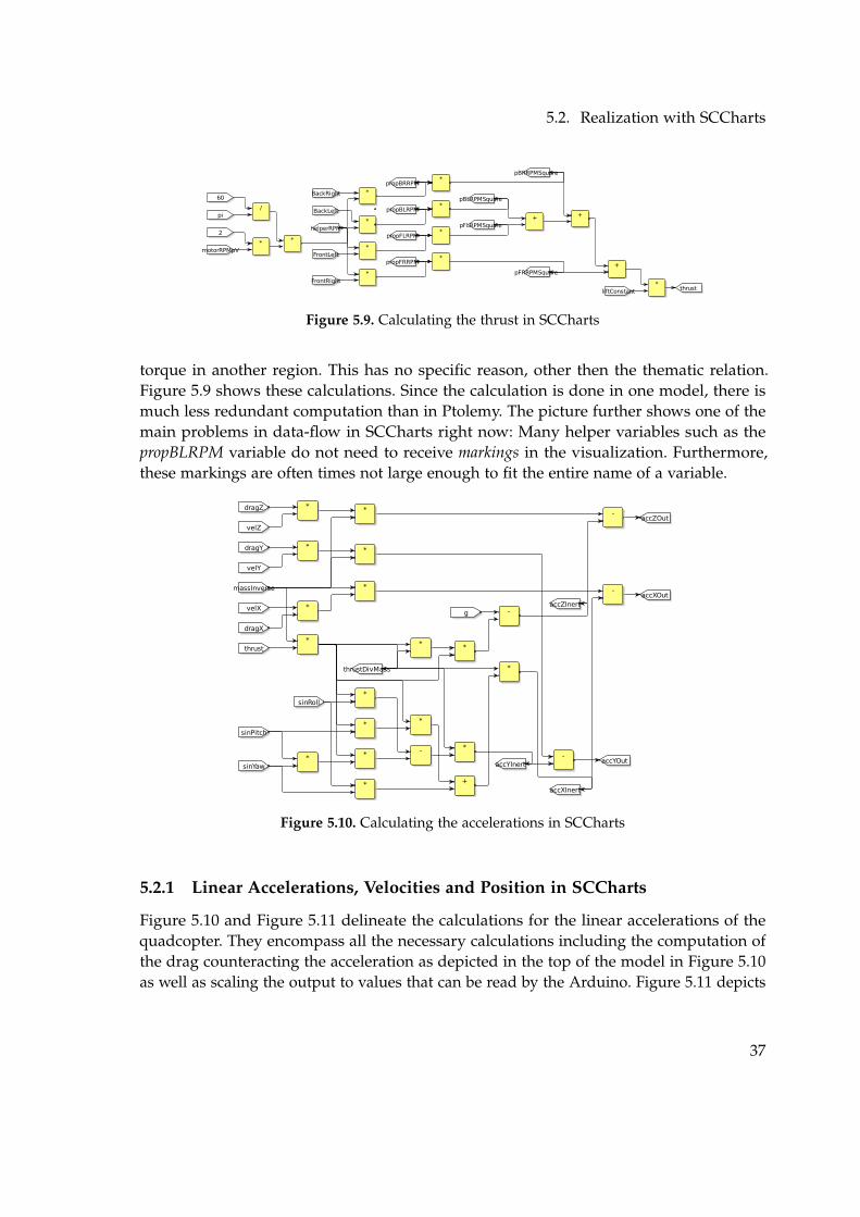
torque in another region. This has no specific reason, other then the thematic relation.Figure 5.9 shows these calculations. Since the calculation is done in one model, there ismuch less redundant computation than in Ptolemy. The picture further shows one of themain problems in data-flow in SCCharts right now: Many helper variables such as thepropBLRPM variable do not need to receive markings in the visualization. Furthermore,these markings are often times not large enough to fit the entire name of a variable.

thrust

massInverse

*

thrustDivMass

sinPitch* *

sinYaw

sinRoll

* +

*

accXInert

* *

*

- *

accYInert

* *

g -accZInert

velX

dragX

*

* -accXOut

velY

dragY * *

-accYOut

velZ

dragZ * * -accZOut

Figure 5.10. Calculating the accelerations in SCCharts

5.2.1 Linear Accelerations, Velocities and Position in SCCharts

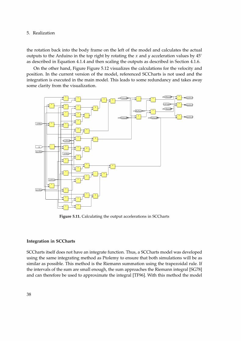
Figure 5.10 and Figure 5.11 delineate the calculations for the linear accelerations of thequadcopter. They encompass all the necessary calculations including the computation ofthe drag counteracting the acceleration as depicted in the top of the model in Figure 5.10as well as scaling the output to values that can be read by the Arduino. Figure 5.11 depicts

37

5. Realization

the rotation back into the body frame on the left of the model and calculates the actualoutputs to the Arduino in the top right by rotating the x and y acceleration values by 450

as described in Equation 4.1.4 and then scaling the outputs as described in Section 4.1.6.

On the other hand, Figure Figure 5.12 visualizes the calculations for the velocity andposition. In the current version of the model, referenced SCCharts is not used and theintegration is executed in the main model. This leads to some redundancy and takes awaysome clarity from the visualization.

accZOut

g-

accXOut

*

*

accYOut

*

sinYaw

* +

sinPitch

* +

accXUnscaled

sinRoll * *

*

* * -

* * * +

* * +

* *

+accYUnscaled

* *

*

* *

+

*

*

*

*

* - +

*

* +

accZUnscaled

-

oneByRootTwo

*accXRotated

+

*accYRotated

scalingAcc

*OutputAccX

*OutputAccY

*OutputAccZ

Figure 5.11. Calculating the output accelerations in SCCharts

Integration in SCCharts

SCCharts itself does not have an integrate function. Thus, a SCCharts model was developedusing the same integrating method as Ptolemy to ensure that both simulations will be assimilar as possible. This method is the Riemann summation using the trapezoidal rule. Ifthe intervals of the sum are small enough, the sum approaches the Riemann integral [SG78]and can therefore be used to approximate the integral [TF96]. With this method the model

38

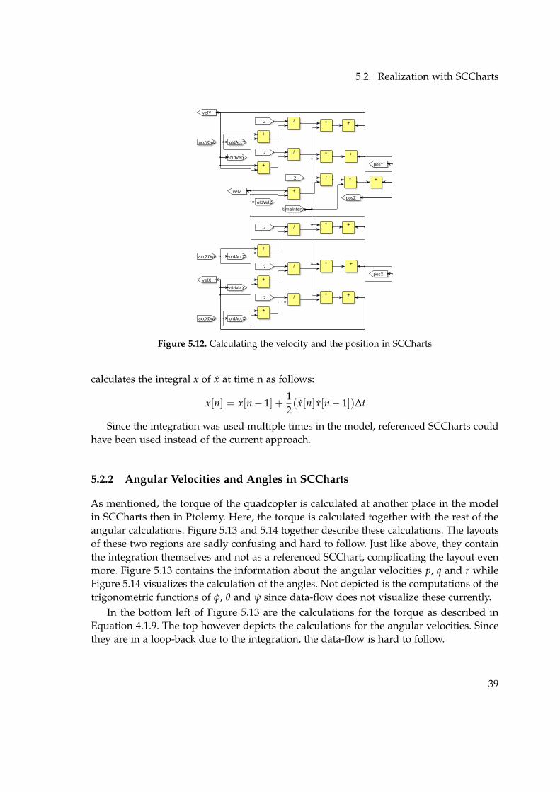
5.2. Realization with SCCharts

velX

timeInterval

oldAccXaccXOut

+

2 / * +

velY

oldAccYaccYOut

+

2 / * +

velZ

oldAccZaccZOut

+

2 / * +

posX

oldVelX

+

2 / * +

posY

oldVelY

+

2 / * +

posZoldVelZ

+

2 / * +

Figure 5.12. Calculating the velocity and the position in SCCharts

calculates the integral x of x at time n as follows:

x[n] = x[n´ 1] +12(x[n]x[n´ 1])∆t

Since the integration was used multiple times in the model, referenced SCCharts couldhave been used instead of the current approach.

5.2.2 Angular Velocities and Angles in SCCharts

As mentioned, the torque of the quadcopter is calculated at another place in the modelin SCCharts then in Ptolemy. Here, the torque is calculated together with the rest of theangular calculations. Figure 5.13 and 5.14 together describe these calculations. The layoutsof these two regions are sadly confusing and hard to follow. Just like above, they containthe integration themselves and not as a referenced SCChart, complicating the layout evenmore. Figure 5.13 contains the information about the angular velocities p, q and r whileFigure 5.14 visualizes the calculation of the angles. Not depicted is the computations of thetrigonometric functions of φ, θ and ψ since data-flow does not visualize these currently.

In the bottom left of Figure 5.13 are the calculations for the torque as described inEquation 4.1.9. The top however depicts the calculations for the angular velocities. Sincethey are in a loop-back due to the integration, the data-flow is hard to follow.

39

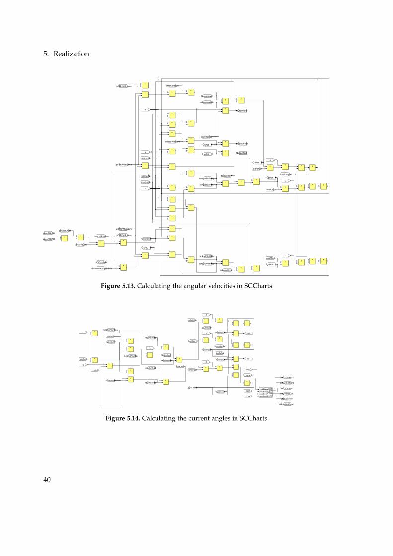
5. Realization

distanceRotorMiddle

liftConstant

*

liftC

pBLRPMSquare

pFRRPMSquare - *

torqueRoll

pBRRPMSquare

pFLRPMSquare

- *

torquePitch

-

-

+

dragConstant

*

torqueYaw

propFRRPM

propBLRPM

propFLRPM

-

propBRRPM

-

+

inertiaRotation

*rotation

q

r

*

inertiaYY

inertiaZZ

-

*torqueRollPos

*

*

torqueRollNeg

p

*

inertiaXX

- *

torquePitchPos

*

*torquePitchNeg

*

-

*

torqueYawPos

- + /pDer

-

+ /qDer

+ /

rDer

timeInterval

oldPDer+

2

/ * +

oldQDer

+

2

/ * +

oldRDer+

2

/ * +

-

oneByRootTwo

*

pRot

+

*

qRot

scalingDeg

*OutputRoll

*OutputPitch

*OutputYaw

Figure 5.13. Calculating the angular velocities in SCCharts

posX

posY

posZ

yaw

[+] Distances

positionXpositionYpositionZyawAnglefront

rightback

leftup

down

cosRoll

rcosRoll

q

sinRoll *

qsinRoll

tanPitch

*helpRotRoll1

*

helpRotRoll2

*

helpRotPitchPos

r *helpRotPitchNeg

/helpRotYaw1

/

helpRotYaw2

p+

+

rollDer

-pitchDer

+

yawDer

rollUnsc

timeInterval

oldRollDer

+

2

/

* +

pitchUnsc

+

2

/

* +

yawUnsc

oldYawDer+

2

/ *

+

rollUnsc2

pitchUnsc2

yawUnsc2

degToRad

*roll

*pitch

*

OutputDistFront

OutputDistBack

OutputDistLeft

OutputDistRight

OutputDistUp

OutputDistDown

Figure 5.14. Calculating the current angles in SCCharts

40

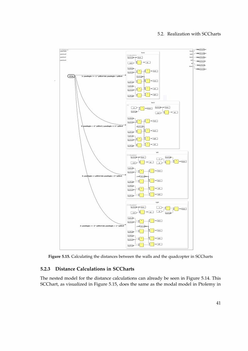
5.2. Realization with SCCharts

[-] Distances

setup

front

[-] calculations

wallFront

positionY

-

yawAngle

/front

wallRight

positionX

- /right

wallBack

+ /back

wallLeft

+ /left

roof

positionZ

-up

down

right

[-] calculations

yawAnglepi

2 / -helper

yawPiHalvesCos

wallRight

positionX

- /front

wallBack

positionY+ /

right

wallLeft

+ /back

wallFront- /

left

roof

positionZ

-up

down

left

[-] calculations

yawAngle

pi

2

/ +helper

yawPiHalvesCos

wallLeft

positionX+ /

front

wallFront

positionY

- /right

wallRight- /

back

wallBack

+ /left

roof

positionZ

-up

down

back

[-]

yawAngle

pi +helper

yawPiCos

wallBack

positionY+ /

front

wallLeft

positionX+ /

right

wallFront- /

back

wallRight- /

left

roof

positionZ

-up

down

1: yawAngle >= -1 * piDiv4 && yawAngle < piDiv4

2: yawAngle >= -3 * piDiv4 && yawAngle < -1 * piDiv4

4: yawAngle >= piDiv4 && yawAngle < 3 * piDiv4

3: yawAngle < -3 * piDiv4 || yawAngle >= 3 * piDiv4

positionX

positionY

positionZ

yawAngle front

right

back

left

up

down

OutputDistFront

OutputDistBack

OutputDistLeft

OutputDistRight

OutputDistUp

OutputDistDown

Figure 5.15. Calculating the distances between the walls and the quadcopter in SCCharts

5.2.3 Distance Calculations in SCCharts

The nested model for the distance calculations can already be seen in Figure 5.14. ThisSCChart, as visualized in Figure 5.15, does the same as the modal model in Ptolemy in

41

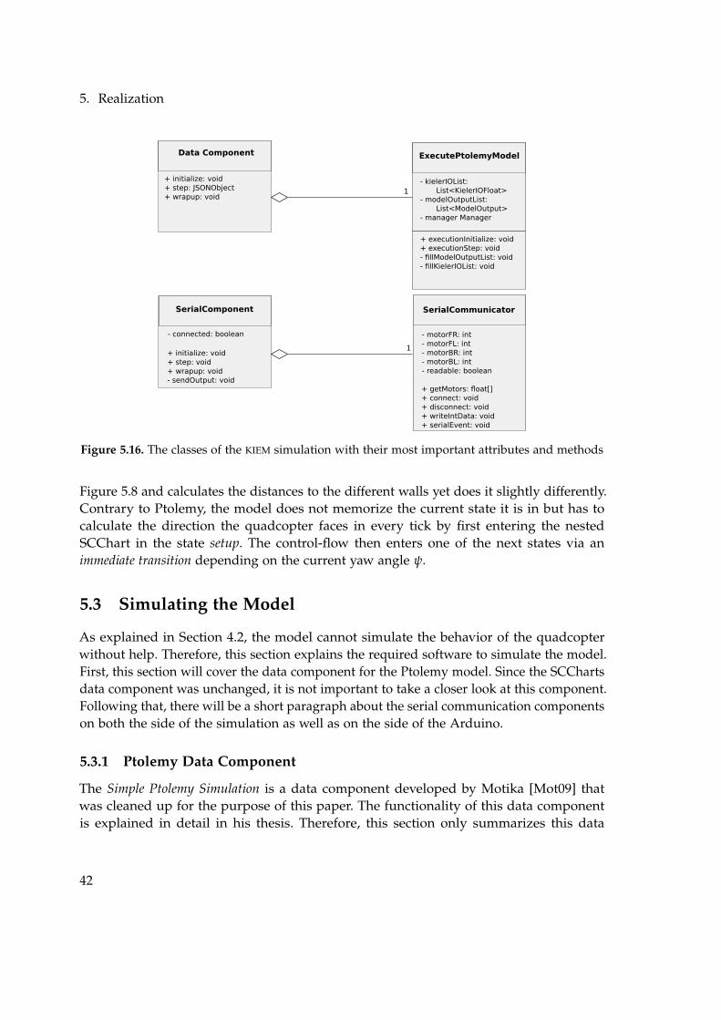
5. Realization

Data Component

+ initialize: void+ step: JSONObject+ wrapup: void

SerialComponent

- connected: boolean

+ initialize: void+ step: void+ wrapup: void- sendOutput: void

SerialCommunicator

- motorFR: int- motorFL: int- motorBR: int- motorBL: int- readable: boolean

+ getMotors: float[]+ connect: void+ disconnect: void+ writeIntData: void+ serialEvent: void

ExecutePtolemyModel

- kielerIOList: List<KielerIOFloat>- modelOutputList: List<ModelOutput>- manager Manager

+ executionInitialize: void+ executionStep: void- fillModelOutputList: void- fillKielerIOList: void

1

1

Figure 5.16. The classes of the KIEM simulation with their most important attributes and methods

Figure 5.8 and calculates the distances to the different walls yet does it slightly differently.Contrary to Ptolemy, the model does not memorize the current state it is in but has tocalculate the direction the quadcopter faces in every tick by first entering the nestedSCChart in the state setup. The control-flow then enters one of the next states via animmediate transition depending on the current yaw angle ψ.

5.3 Simulating the Model

As explained in Section 4.2, the model cannot simulate the behavior of the quadcopterwithout help. Therefore, this section explains the required software to simulate the model.First, this section will cover the data component for the Ptolemy model. Since the SCChartsdata component was unchanged, it is not important to take a closer look at this component.Following that, there will be a short paragraph about the serial communication componentson both the side of the simulation as well as on the side of the Arduino.

5.3.1 Ptolemy Data Component

The Simple Ptolemy Simulation is a data component developed by Motika [Mot09] thatwas cleaned up for the purpose of this paper. The functionality of this data componentis explained in detail in his thesis. Therefore, this section only summarizes this data

42

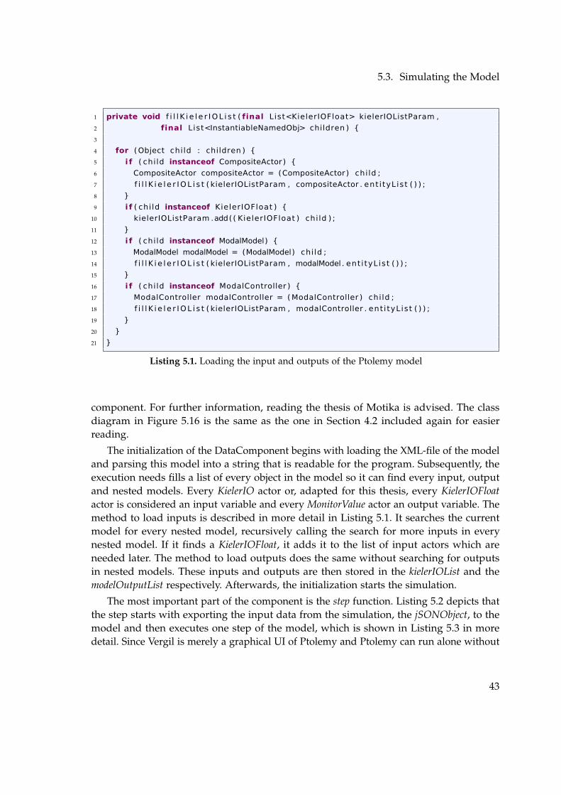
5.3. Simulating the Model

1 private void f i l l K i e l e r IOL i s t ( final List<KielerIOFloat> kielerIOListParam ,

2 final List<InstantiableNamedObj> children ) {

3

4 for (Object child : children ) {

5 i f ( chi ld instanceof CompositeActor ) {

6 CompositeActor compositeActor = (CompositeActor ) child ;

7 f i l l K i e l e r IOL i s t ( kielerIOListParam , compositeActor . ent i tyL ist ( ) ) ;

8 }

9 i f ( chi ld instanceof KielerIOFloat ) {

10 kielerIOListParam .add( ( KielerIOFloat ) child ) ;

11 }

12 i f ( chi ld instanceof ModalModel) {

13 ModalModel modalModel = (ModalModel) child ;

14 f i l l K i e l e r IOL i s t ( kielerIOListParam , modalModel . ent i tyL ist ( ) ) ;

15 }

16 i f ( chi ld instanceof ModalController ) {

17 ModalController modalController = (ModalController ) child ;

18 f i l l K i e l e r IOL i s t ( kielerIOListParam , modalController . ent i tyL ist ( ) ) ;

19 }

20 }

21 }

Listing 5.1. Loading the input and outputs of the Ptolemy model

component. For further information, reading the thesis of Motika is advised. The classdiagram in Figure 5.16 is the same as the one in Section 4.2 included again for easierreading.

The initialization of the DataComponent begins with loading the XML-file of the modeland parsing this model into a string that is readable for the program. Subsequently, theexecution needs fills a list of every object in the model so it can find every input, outputand nested models. Every KielerIO actor or, adapted for this thesis, every KielerIOFloatactor is considered an input variable and every MonitorValue actor an output variable. Themethod to load inputs is described in more detail in Listing 5.1. It searches the currentmodel for every nested model, recursively calling the search for more inputs in everynested model. If it finds a KielerIOFloat, it adds it to the list of input actors which areneeded later. The method to load outputs does the same without searching for outputsin nested models. These inputs and outputs are then stored in the kielerIOList and themodelOutputList respectively. Afterwards, the initialization starts the simulation.

The most important part of the component is the step function. Listing 5.2 depicts thatthe step starts with exporting the input data from the simulation, the jSONObject, to themodel and then executes one step of the model, which is shown in Listing 5.3 in moredetail. Since Vergil is merely a graphical UI of Ptolemy and Ptolemy can run alone without

43

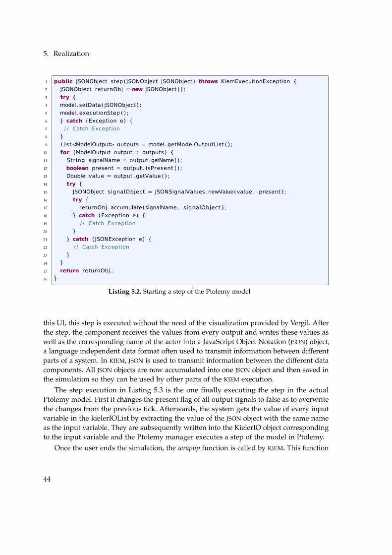
5. Realization

1 public JSONObject step ( JSONObject jSONObject ) throws KiemExecutionException {

2 JSONObject returnObj = new JSONObject ( ) ;

3 try {

4 model . setData( jSONObject ) ;

5 model . executionStep ( ) ;

6 } catch (Exception e) {

7 / / Catch Exception

8 }

9 List<ModelOutput> outputs = model . getModelOutputList ( ) ;

10 for (ModelOutput output : outputs ) {

11 String signalName = output .getName( ) ;

12 boolean present = output . isPresent ( ) ;

13 Double value = output . getValue ( ) ;

14 try {

15 JSONObject signalObject = JSONSignalValues .newValue(value , present ) ;

16 try {

17 returnObj . accumulate(signalName , signalObject ) ;

18 } catch (Exception e) {

19 / / Catch Exception

20 }

21 } catch ( JSONException e) {

22 / / Catch Exception

23 }

24 }

25 return returnObj ;

26 }

Listing 5.2. Starting a step of the Ptolemy model

this UI, this step is executed without the need of the visualization provided by Vergil. Afterthe step, the component receives the values from every output and writes these values aswell as the corresponding name of the actor into a JavaScript Object Notation (JSON) object,a language independent data format often used to transmit information between differentparts of a system. In KIEM, JSON is used to transmit information between the different datacomponents. All JSON objects are now accumulated into one JSON object and then saved inthe simulation so they can be used by other parts of the KIEM execution.

The step execution in Listing 5.3 is the one finally executing the step in the actualPtolemy model. First it changes the present flag of all output signals to false as to overwritethe changes from the previous tick. Afterwards, the system gets the value of every inputvariable in the kielerIOList by extracting the value of the JSON object with the same nameas the input variable. They are subsequently written into the KielerIO object correspondingto the input variable and the Ptolemy manager executes a step of the model in Ptolemy.

Once the user ends the simulation, the wrapup function is called by KIEM. This function

44

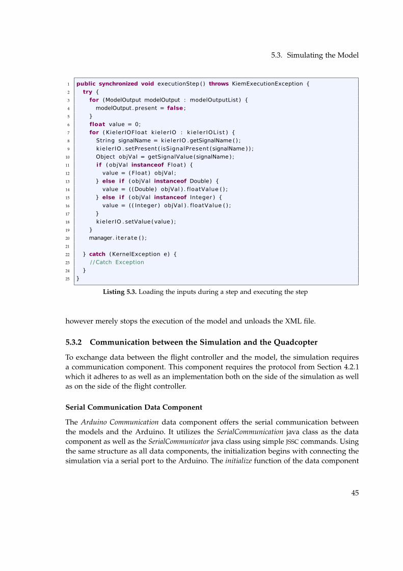
5.3. Simulating the Model

1 public synchronized void executionStep ( ) throws KiemExecutionException {

2 try {

3 for (ModelOutput modelOutput : modelOutputList ) {

4 modelOutput . present = false ;

5 }

6 float value = 0;

7 for ( KielerIOFloat kielerIO : k ie ler IOList ) {

8 String signalName = kielerIO .getSignalName ( ) ;

9 kielerIO . setPresent ( isSignalPresent (signalName ) ) ;

10 Object objVal = getSignalValue (signalName ) ;

11 i f ( objVal instanceof Float ) {

12 value = ( Float ) objVal ;

13 } else i f ( objVal instanceof Double) {

14 value = ((Double) objVal ) . floatValue ( ) ;

15 } else i f ( objVal instanceof Integer ) {

16 value = (( Integer ) objVal ) . floatValue ( ) ;

17 }

18 kielerIO . setValue (value ) ;

19 }

20 manager. iterate ( ) ;

21

22 } catch ( KernelException e) {

23 / / Catch Exception

24 }

25 }

Listing 5.3. Loading the inputs during a step and executing the step

however merely stops the execution of the model and unloads the XML file.

5.3.2 Communication between the Simulation and the Quadcopter

To exchange data between the flight controller and the model, the simulation requiresa communication component. This component requires the protocol from Section 4.2.1which it adheres to as well as an implementation both on the side of the simulation as wellas on the side of the flight controller.

Serial Communication Data Component

The Arduino Communication data component offers the serial communication betweenthe models and the Arduino. It utilizes the SerialCommunication java class as the datacomponent as well as the SerialCommunicator java class using simple JSSC commands. Usingthe same structure as all data components, the initialization begins with connecting thesimulation via a serial port to the Arduino. The initialize function of the data component

45

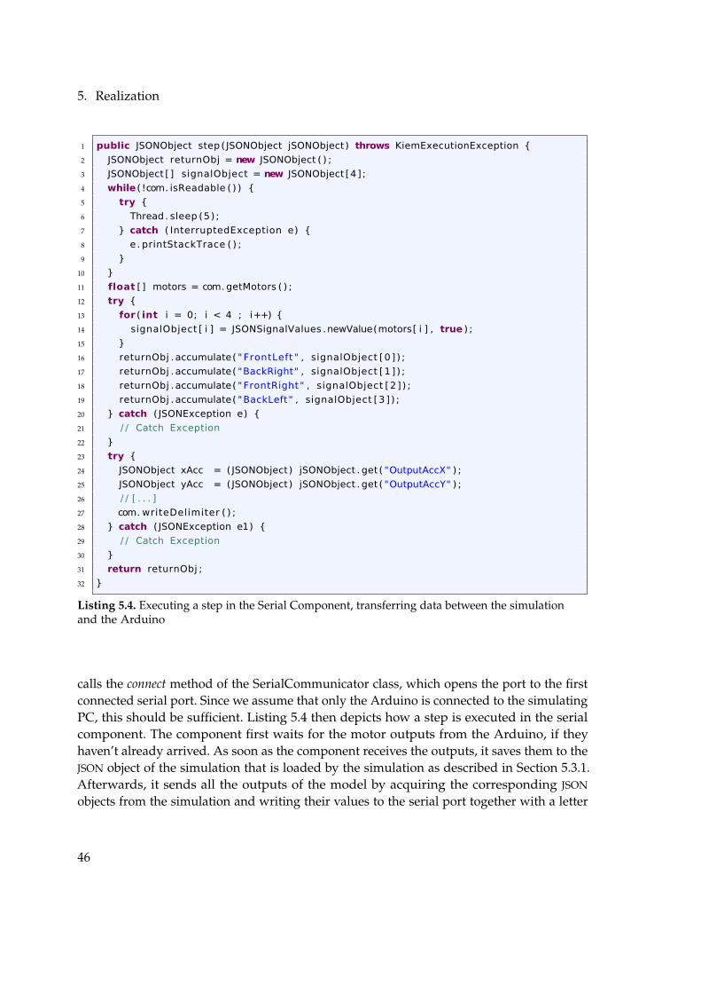
5. Realization

1 public JSONObject step ( JSONObject jSONObject ) throws KiemExecutionException {

2 JSONObject returnObj = new JSONObject ( ) ;

3 JSONObject [ ] signalObject = new JSONObject [4] ;

4 while ( !com. isReadable ( ) ) {

5 try {

6 Thread . sleep (5) ;

7 } catch ( InterruptedException e) {

8 e. printStackTrace ( ) ;

9 }

10 }

11 float [ ] motors = com.getMotors ( ) ;

12 try {

13 for ( int i = 0; i < 4 ; i++) {

14 signalObject [ i ] = JSONSignalValues .newValue(motors[ i ] , true ) ;

15 }

16 returnObj . accumulate( " FrontLeft " , signalObject [0 ] ) ;

17 returnObj . accumulate( "BackRight" , signalObject [1 ] ) ;

18 returnObj . accumulate( "FrontRight" , signalObject [2 ] ) ;

19 returnObj . accumulate( "BackLeft" , signalObject [3 ] ) ;

20 } catch ( JSONException e) {

21 / / Catch Exception

22 }

23 try {

24 JSONObject xAcc = ( JSONObject ) jSONObject . get ( "OutputAccX" ) ;

25 JSONObject yAcc = ( JSONObject ) jSONObject . get ( "OutputAccY" ) ;

26 / / [ . . . ]

27 com. writeDelimiter ( ) ;

28 } catch ( JSONException e1) {

29 / / Catch Exception

30 }

31 return returnObj ;

32 }

Listing 5.4. Executing a step in the Serial Component, transferring data between the simulationand the Arduino

calls the connect method of the SerialCommunicator class, which opens the port to the firstconnected serial port. Since we assume that only the Arduino is connected to the simulatingPC, this should be sufficient. Listing 5.4 then depicts how a step is executed in the serialcomponent. The component first waits for the motor outputs from the Arduino, if theyhaven’t already arrived. As soon as the component receives the outputs, it saves them to theJSON object of the simulation that is loaded by the simulation as described in Section 5.3.1.Afterwards, it sends all the outputs of the model by acquiring the corresponding JSON

objects from the simulation and writing their values to the serial port together with a letter

46

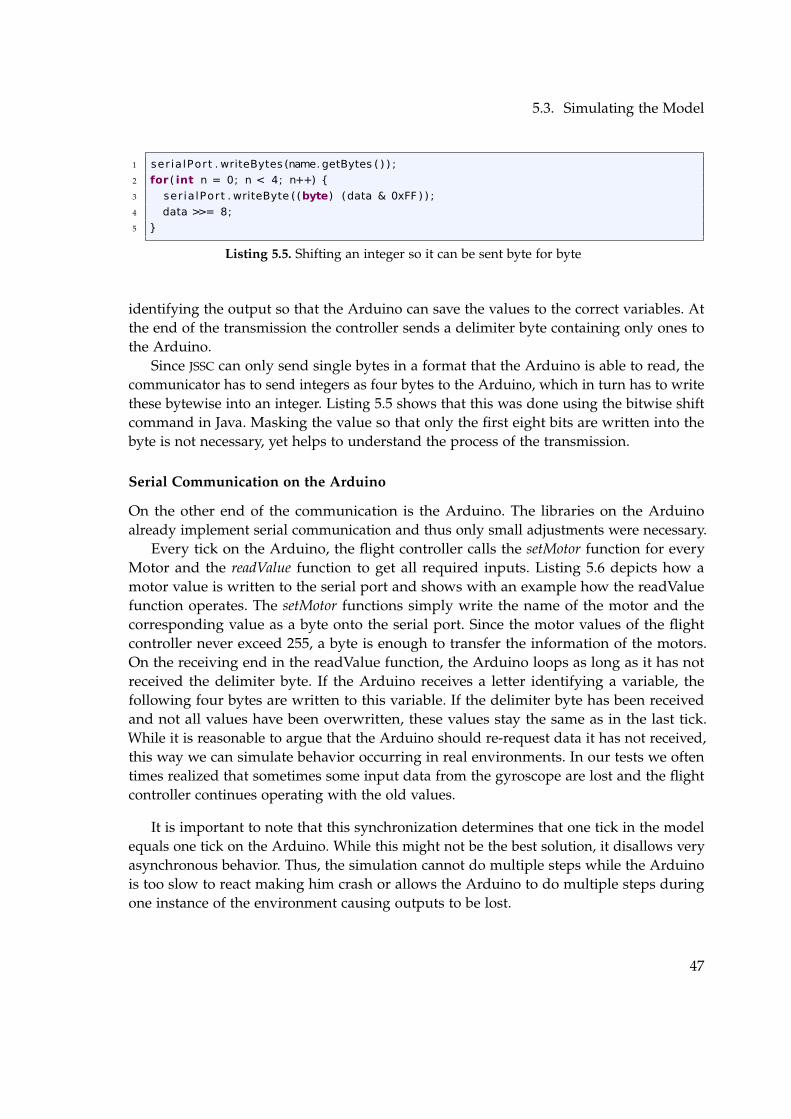
5.3. Simulating the Model

1 serialPort . writeBytes (name. getBytes ( ) ) ;

2 for ( int n = 0; n < 4; n++) {

3 serialPort . writeByte ( (byte) (data & 0xFF ) ) ;

4 data >>= 8;

5 }

Listing 5.5. Shifting an integer so it can be sent byte for byte

identifying the output so that the Arduino can save the values to the correct variables. Atthe end of the transmission the controller sends a delimiter byte containing only ones tothe Arduino.

Since JSSC can only send single bytes in a format that the Arduino is able to read, thecommunicator has to send integers as four bytes to the Arduino, which in turn has to writethese bytewise into an integer. Listing 5.5 shows that this was done using the bitwise shiftcommand in Java. Masking the value so that only the first eight bits are written into thebyte is not necessary, yet helps to understand the process of the transmission.

Serial Communication on the Arduino

On the other end of the communication is the Arduino. The libraries on the Arduinoalready implement serial communication and thus only small adjustments were necessary.

Every tick on the Arduino, the flight controller calls the setMotor function for everyMotor and the readValue function to get all required inputs. Listing 5.6 depicts how amotor value is written to the serial port and shows with an example how the readValuefunction operates. The setMotor functions simply write the name of the motor and thecorresponding value as a byte onto the serial port. Since the motor values of the flightcontroller never exceed 255, a byte is enough to transfer the information of the motors.On the receiving end in the readValue function, the Arduino loops as long as it has notreceived the delimiter byte. If the Arduino receives a letter identifying a variable, thefollowing four bytes are written to this variable. If the delimiter byte has been receivedand not all values have been overwritten, these values stay the same as in the last tick.While it is reasonable to argue that the Arduino should re-request data it has not received,this way we can simulate behavior occurring in real environments. In our tests we oftentimes realized that sometimes some input data from the gyroscope are lost and the flightcontroller continues operating with the old values.

It is important to note that this synchronization determines that one tick in the modelequals one tick on the Arduino. While this might not be the best solution, it disallows veryasynchronous behavior. Thus, the simulation cannot do multiple steps while the Arduinois too slow to react making him crash or allows the Arduino to do multiple steps duringone instance of the environment causing outputs to be lost.

47

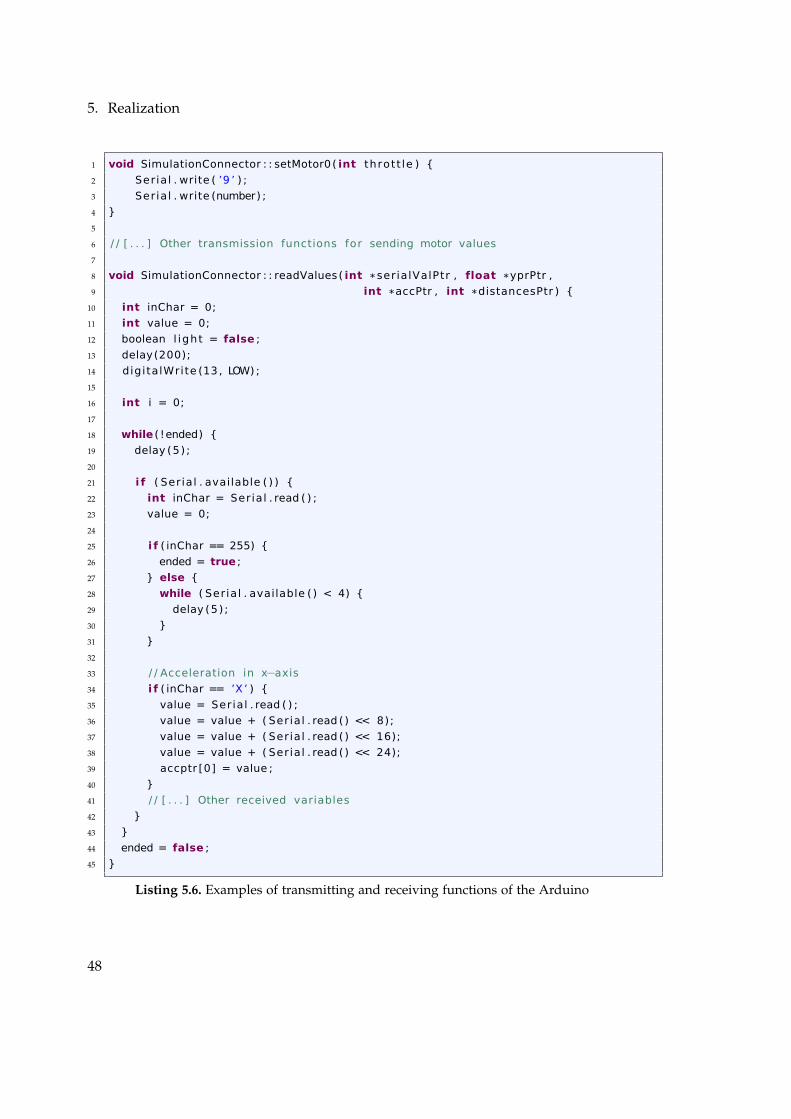
5. Realization

1 void SimulationConnector : : setMotor0( int thrott le ) {

2 Serial . write ( ’9 ’ ) ;

3 Serial . write (number) ;

4 }

5

6 / / [ . . . ] Other transmission functions for sending motor values

7

8 void SimulationConnector : : readValues( int * serialValPtr , float *yprPtr ,

9 int *accPtr , int *distancesPtr ) {

10 int inChar = 0;

11 int value = 0;

12 boolean l ight = false ;

13 delay(200);

14 digitalWrite (13 , LOW) ;

15

16 int i = 0;

17

18 while ( !ended) {

19 delay (5) ;

20

21 i f ( Serial . available ( ) ) {

22 int inChar = Serial . read ( ) ;

23 value = 0;

24

25 i f ( inChar == 255) {

26 ended = true ;

27 } else {

28 while ( Serial . available ( ) < 4) {

29 delay (5) ;

30 }

31 }

32

33 / / Acceleration in x axis

34 i f ( inChar == ’X ’ ) {

35 value = Serial . read ( ) ;

36 value = value + ( Serial . read ( ) << 8);

37 value = value + ( Serial . read ( ) << 16);

38 value = value + ( Serial . read ( ) << 24);

39 accptr [0] = value ;

40 }

41 / / [ . . . ] Other received variables

42 }

43 }

44 ended = false ;

45 }

Listing 5.6. Examples of transmitting and receiving functions of the Arduino

48

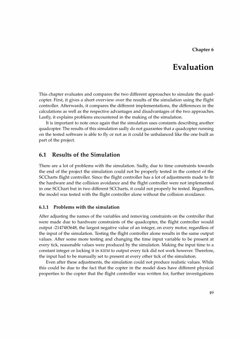
Chapter 6

Evaluation

This chapter evaluates and compares the two different approaches to simulate the quad-copter. First, it gives a short overview over the results of the simulation using the flightcontroller. Afterwards, it compares the different implementations, the differences in thecalculations as well as the respective advantages and disadvantages of the two approaches.Lastly, it explains problems encountered in the making of the simulation.

It is important to note once again that the simulation uses constants describing anotherquadcopter. The results of this simulation sadly do not guarantee that a quadcopter runningon the tested software is able to fly or not as it could be unbalanced like the one built aspart of the project.

6.1 Results of the Simulation

There are a lot of problems with the simulation. Sadly, due to time constraints towardsthe end of the project the simulation could not be properly tested in the context of theSCCharts flight controller. Since the flight controller has a lot of adjustments made to fitthe hardware and the collision avoidance and the flight controller were not implementedin one SCChart but in two different SCCharts, it could not properly be tested. Regardless,the model was tested with the flight controller alone without the collision avoidance.

6.1.1 Problems with the simulation

After adjusting the names of the variables and removing constraints on the controller thatwere made due to hardware constraints of the quadcopter, the flight controller wouldoutput -2147483648, the largest negative value of an integer, on every motor, regardless ofthe input of the simulation. Testing the flight controller alone results in the same outputvalues. After some more testing and changing the time input variable to be present atevery tick, reasonable values were produced by the simulation. Making the input time to aconstant integer or locking it in KIEM to output every tick did not work however. Therefore,the input had to be manually set to present at every other tick of the simulation.

Even after these adjustments, the simulation could not produce realistic values. Whilethis could be due to the fact that the copter in the model does have different physicalproperties to the copter that the flight controller was written for, further investigations

49

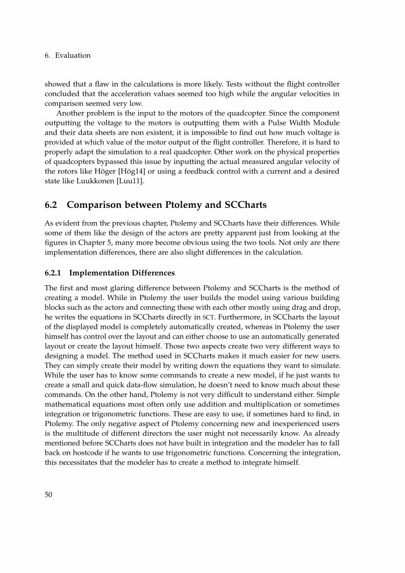
6. Evaluation

showed that a flaw in the calculations is more likely. Tests without the flight controllerconcluded that the acceleration values seemed too high while the angular velocities incomparison seemed very low.

Another problem is the input to the motors of the quadcopter. Since the componentoutputting the voltage to the motors is outputting them with a Pulse Width Moduleand their data sheets are non existent, it is impossible to find out how much voltage isprovided at which value of the motor output of the flight controller. Therefore, it is hard toproperly adapt the simulation to a real quadcopter. Other work on the physical propertiesof quadcopters bypassed this issue by inputting the actual measured angular velocity ofthe rotors like Höger [Hög14] or using a feedback control with a current and a desiredstate like Luukkonen [Luu11].

6.2 Comparison between Ptolemy and SCCharts

As evident from the previous chapter, Ptolemy and SCCharts have their differences. Whilesome of them like the design of the actors are pretty apparent just from looking at thefigures in Chapter 5, many more become obvious using the two tools. Not only are thereimplementation differences, there are also slight differences in the calculation.

6.2.1 Implementation Differences

The first and most glaring difference between Ptolemy and SCCharts is the method ofcreating a model. While in Ptolemy the user builds the model using various buildingblocks such as the actors and connecting these with each other mostly using drag and drop,he writes the equations in SCCharts directly in SCT. Furthermore, in SCCharts the layoutof the displayed model is completely automatically created, whereas in Ptolemy the userhimself has control over the layout and can either choose to use an automatically generatedlayout or create the layout himself. Those two aspects create two very different ways todesigning a model. The method used in SCCharts makes it much easier for new users.They can simply create their model by writing down the equations they want to simulate.While the user has to know some commands to create a new model, if he just wants tocreate a small and quick data-flow simulation, he doesn’t need to know much about thesecommands. On the other hand, Ptolemy is not very difficult to understand either. Simplemathematical equations most often only use addition and multiplication or sometimesintegration or trigonometric functions. These are easy to use, if sometimes hard to find, inPtolemy. The only negative aspect of Ptolemy concerning new and inexperienced usersis the multitude of different directors the user might not necessarily know. As alreadymentioned before SCCharts does not have built in integration and the modeler has to fallback on hostcode if he wants to use trigonometric functions. Concerning the integration,this necessitates that the modeler has to create a method to integrate himself.

50

6.2. Comparison between Ptolemy and SCCharts

+

liftConstant

*

thrust

massInverse *thrustDivMass

* *

sinYaw

*

+ *

accXInert

*

*

*

- *

accYInert

* * -accZInert

velX

dragX * * -

accXOut

velY

dragY

*

* -

velZ

dragZ *

* -

accZOut

timeInterval

oldAccZ

+

2 /

*

posX

oldVelX

+

2 /

* +

posY

oldVelY

+

2 / * +

posZ

oldVelZ

+

2 /

* +

* +

* * *

*

*

oneByRootTwo

-

+

torqueYaw

q

p

inertiaXX

*

-

*

torqueYawPos

+

/

rDer

oldRDer +

2 /

* +

-

*

pRot

+ *

qRot

scalingDeg

*OutputRoll

*OutputPitch

Figure 6.1. A very cluttered and unclear part of the model in SCCharts

Since SCCharts creates the layout for the user, he does not need to focus on creating agood layout. Sadly, the data-flow layout in SCCharts is often times not very clear, especiallyfor large models. The modeler can choose to create one big model that contains everythingmaintaining all connections like in Figure 6.1 or create multiple small regions like inFigure 6.2. While the second option maintains a clearer layout, it loses some relationsbetween some components. For example, in Figure 6.2, the actor ’AccZOut’ in the top leftof the region ’CalculateAccelerations’ is an output that is required as an input in the region’CalculateVelocityAndPosition’ on the left. A visually better option as depicted in Figure 6.3is to create nested SCCharts containing a single state that then contains the equations in adata-flow environment. The picture shows two parts of the model, one opened and anotherone closed. Sadly, the inputs are still not completely connected to the actual actors. Whilethis also creates a lot of work for the modeler it is probably the best option as unnecessaryinformation can be hidden and a lot of clutter can be removed from the model.

On the other hand, Ptolemy users can create their own vision of the model. Actors andcomposite models can be moved around manually and a good modeler can create a modelthat is clear and can be understood very easily. This of course can take up a lot of time andeffort the modeler does not necessarily have to expend. Alternatively, Ptolemy offers thepossibility to layout the model automatically as mentioned above. This automatic layoutis generated by the KLay Layered algorithm from the KIELER project [SSH14]. SCCharts

51

6. Evaluation

*thrust

[-] CalculateAccelerations

thrust

massInverse

*

thrustDivMass

sinPitch* *

sinYaw

sinRoll

* +

*

accXInert

* *

*

- *

accYInert

* *

g -accZInert

velX

dragX

*

* -accXOut

velY

dragY * *

-accYOut

velZ

dragZ * * -accZOut

[-] calculateVelocityAndPosition

velX

timeInterval

oldAccXaccXOut

+

2 / * +

velY

oldAccYaccYOut

+

2 / * +

velZ

oldAccZaccZOut

+

2 / * +

posX

oldVelX

+

2 / * +

posY

oldVelY

+

2 / * +

posZoldVelZ

+

2 / * +

[-] calculateActualAccelerations

accXUnscaled

sinRoll * *

*

* * -

* * * +

* * +

* *

+accYUnscaled

accZUnscaled

-

oneByRootTwo

*accXRotated

+

*accYRotated

scalingAcc

*OutputAccX

*OutputAccY

*OutputAccZ

+

+

roll

pitch

Figure 6.2. Data-flow divided into different regions

FrontRight

FrontLeft

BackRight

BackLeft [-] calculateThrust

calcs

[-] CalculateThrust

motorRPMpV

2

*

pi

60

/

*

helperRPM

FR*

propFRRPMFL

*

propFLRPM

BR *

propBRRPM

BL

*

propBLRPM

*

pFRRPMSquare

*pFLRPMSquare

*pBRRPMSquare

*pBLRPMSquare

+ +

+

liftConstant*

thrustOut

FR

FL

BR

BL thrustOut thrust

[+] CalculateAccelerations

thrust

accXOut

accYOut

accZOut

accXOut

accYOut

accZOut

Figure 6.3. Two different data-flow regions in nested SCCharts with variables that carry over

however does not offer the possibility to manually edit the layout of a model.Another important aspect of modeling is reusing parts of a model. Instead of using a

copy and paste approach, it is often of advantage to create a way to reuse a part of themodel in another place, while still maintaining the information that this part of the modelis a copy of the original. This way, fixing a mistake in the original can also fix the mistakein the copy. Otherwise, the modeler might have to repair multiple chunks of the model.This kind of feature is implemented both in Ptolemy by converting an actor to a class andthen creating instances of this class as well as in SCCharts via referenced SCCharts.

6.2.2 Differences in Calculations

One big difference in the calculation could be the order of computation. In data-flowin SCCharts it is pretty clear which computation comes before which computation and

52

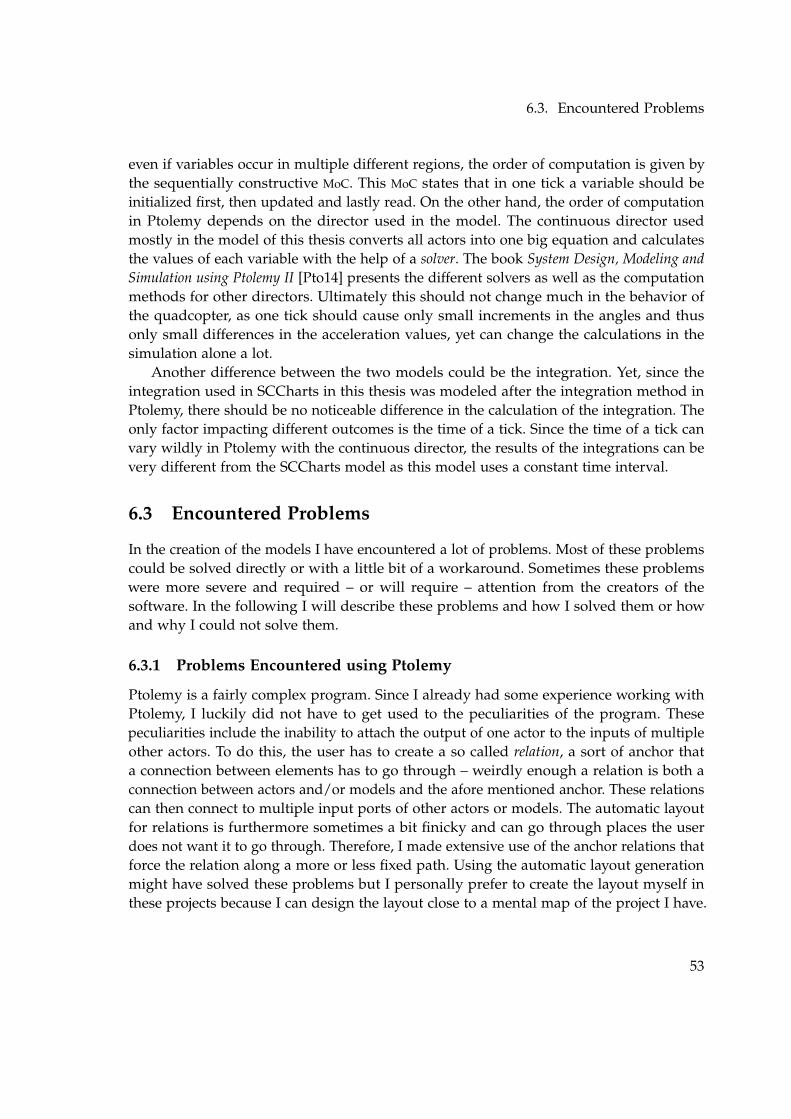
6.3. Encountered Problems

even if variables occur in multiple different regions, the order of computation is given bythe sequentially constructive MoC. This MoC states that in one tick a variable should beinitialized first, then updated and lastly read. On the other hand, the order of computationin Ptolemy depends on the director used in the model. The continuous director usedmostly in the model of this thesis converts all actors into one big equation and calculatesthe values of each variable with the help of a solver. The book System Design, Modeling andSimulation using Ptolemy II [Pto14] presents the different solvers as well as the computationmethods for other directors. Ultimately this should not change much in the behavior ofthe quadcopter, as one tick should cause only small increments in the angles and thusonly small differences in the acceleration values, yet can change the calculations in thesimulation alone a lot.

Another difference between the two models could be the integration. Yet, since theintegration used in SCCharts in this thesis was modeled after the integration method inPtolemy, there should be no noticeable difference in the calculation of the integration. Theonly factor impacting different outcomes is the time of a tick. Since the time of a tick canvary wildly in Ptolemy with the continuous director, the results of the integrations can bevery different from the SCCharts model as this model uses a constant time interval.

6.3 Encountered Problems

In the creation of the models I have encountered a lot of problems. Most of these problemscould be solved directly or with a little bit of a workaround. Sometimes these problemswere more severe and required – or will require – attention from the creators of thesoftware. In the following I will describe these problems and how I solved them or howand why I could not solve them.

6.3.1 Problems Encountered using Ptolemy

Ptolemy is a fairly complex program. Since I already had some experience working withPtolemy, I luckily did not have to get used to the peculiarities of the program. Thesepeculiarities include the inability to attach the output of one actor to the inputs of multipleother actors. To do this, the user has to create a so called relation, a sort of anchor thata connection between elements has to go through – weirdly enough a relation is both aconnection between actors and/or models and the afore mentioned anchor. These relationscan then connect to multiple input ports of other actors or models. The automatic layoutfor relations is furthermore sometimes a bit finicky and can go through places the userdoes not want it to go through. Therefore, I made extensive use of the anchor relations thatforce the relation along a more or less fixed path. Using the automatic layout generationmight have solved these problems but I personally prefer to create the layout myself inthese projects because I can design the layout close to a mental map of the project I have.

53

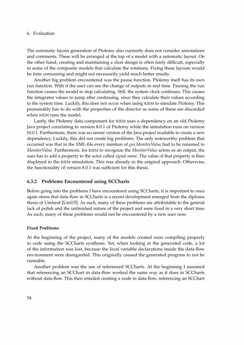
6. Evaluation

The automatic layout generation of Ptolemy also currently does not consider annotationsand comments. These will be arranged at the top of a model with a automatic layout. Onthe other hand, creating and maintaining a clear design is often fairly difficult, especiallyin some of the composite models that calculate the rotations. Fixing these layouts wouldbe time consuming and might not necessarily yield much better results.

Another big problem encountered was the pause function. Ptolemy itself has its ownrun function. With it the user can see the change of outputs in real time. Pausing the runfunction causes the model to stop calculating. Still, the system clock continues. This causesthe integrator values to jump after continuing, since they calculate their values accordingto the system time. Luckily, this does not occur when using KIEM to simulate Ptolemy. Thispresumably has to do with the properties of the director as some of these are discardedwhen KIEM runs the model.

Lastly, the Ptolemy data component for KIEM uses a dependency on an old PtolemyJava project correlating to version 8.0.1 of Ptolemy while the simulation runs on version10.0.1. Furthermore, there was no newer version of the Java project available to create a newdependency. Luckily, this did not create big problems. The only noteworthy problem thatoccurred was that in the XML-file every mention of gui.MonitorValue had to be renamed toMonitorValue. Furthermore, for KIEM to recognize the MonitorValue actors as an output, theuser has to add a property to the actor called signal name. The value of that property is thendisplayed in the KIEM simulation. This was already in the original approach. Otherwise,the functionality of version 8.0.1 was sufficient for this thesis.

6.3.2 Problems Encountered using SCCharts

Before going into the problems I have encountered using SCCharts, it is important to onceagain stress that data-flow in SCCharts is a recent development emerged from the diplomathesis of Umland [Uml15]. As such, many of these problems are attributable to the generallack of polish and the unfinished nature of the project and were fixed in a very short time.As such, many of these problems would not be encountered by a new user now.

Fixed Problems

At the beginning of the project, many of the models created were compiling properlyto code using the SCCharts synthesis. Yet, when looking at the generated code, a lotof the information was lost, because the local variable declarations inside the data-flowenvironment were disregarded. This originally caused the generated program to not berunnable.

Another problem was the use of referenced SCCharts. At the beginning I assumedthat referencing an SCChart in data-flow worked the same way as it does in SCChartswithout data-flow. This then entailed creating a node in data-flow, referencing an SCChart

54

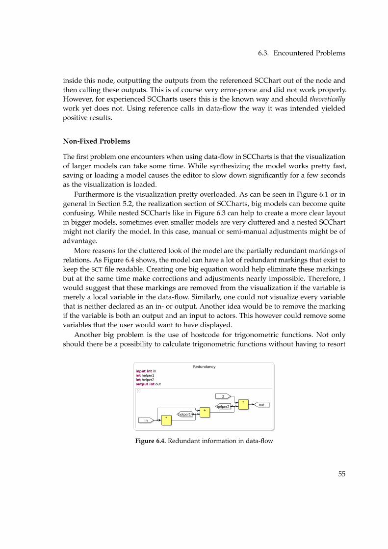
6.3. Encountered Problems

inside this node, outputting the outputs from the referenced SCChart out of the node andthen calling these outputs. This is of course very error-prone and did not work properly.However, for experienced SCCharts users this is the known way and should theoreticallywork yet does not. Using reference calls in data-flow the way it was intended yieldedpositive results.

Non-Fixed Problems

The first problem one encounters when using data-flow in SCCharts is that the visualizationof larger models can take some time. While synthesizing the model works pretty fast,saving or loading a model causes the editor to slow down significantly for a few secondsas the visualization is loaded.

Furthermore is the visualization pretty overloaded. As can be seen in Figure 6.1 or ingeneral in Section 5.2, the realization section of SCCharts, big models can become quiteconfusing. While nested SCCharts like in Figure 6.3 can help to create a more clear layoutin bigger models, sometimes even smaller models are very cluttered and a nested SCChartmight not clarify the model. In this case, manual or semi-manual adjustments might be ofadvantage.

More reasons for the cluttered look of the model are the partially redundant markings ofrelations. As Figure 6.4 shows, the model can have a lot of redundant markings that exist tokeep the SCT file readable. Creating one big equation would help eliminate these markingsbut at the same time make corrections and adjustments nearly impossible. Therefore, Iwould suggest that these markings are removed from the visualization if the variable ismerely a local variable in the data-flow. Similarly, one could not visualize every variablethat is neither declared as an in- or output. Another idea would be to remove the markingif the variable is both an output and an input to actors. This however could remove somevariables that the user would want to have displayed.

Another big problem is the use of hostcode for trigonometric functions. Not onlyshould there be a possibility to calculate trigonometric functions without having to resort

Redundancy input int inint helper1int helper2output int out

[-]

in*

helper1+

helper2

2

*out

Figure 6.4. Redundant information in data-flow

55

6. Evaluation

1 scchart Hostcode {

2 input int in ;

3 output int out ;

4 int helper ;

5

6 dataflow test :

7 helper = <sin ( in )>;

8 out = ’ sin ( helper ) ’ ;

9 }

(a) Hostcode implementations in SCCharts data-flow

HostcodeTest input int in1output int outint helper

[-] test

helper

out

(b) Hostcode disappearing in data-flow

Figure 6.5. Hostcode in SCCharts data-flow

test input int in1input int in2input int in3input int in4input int in5input int in6input int in7input int in8input int in9output int out1output int out2

[-] data

in1

in2

in3

in4

in5

in6

in7

in8

[+] innerNode

in1in2in3longInputOnTheLeftSidein4in5in7in8 out1

out2out3out4

longerOutputOnTheRightSide out1

Figure 6.6. Cluttered inner node with too much text

to hostcode, currently hostcode is not even visualized in data-flow as Figure 6.5 shows.This occurs because the synthesis disregards the contents of the hostcode calls and simplyforwards the code until the end of the synthesis and therefore does not know if anyvariables of the model are being used in the hostcode.

Even more visualization issues occur when using nested or referenced nodes insidedata-flow. When the modeler adds more input or output variables or uses very long namesfor the variables, the size of the node does not change while it is closed. This leads to verycluttered nodes as in Figure 6.6 and prevents the user from opening the node to look at thecontents of it as there are too many labels overlapping to click the button to open the node.

56

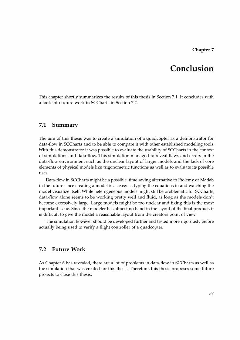
Chapter 7

Conclusion

This chapter shortly summarizes the results of this thesis in Section 7.1. It concludes witha look into future work in SCCharts in Section 7.2.

7.1 Summary

The aim of this thesis was to create a simulation of a quadcopter as a demonstrator fordata-flow in SCCharts and to be able to compare it with other established modeling tools.With this demonstrator it was possible to evaluate the usability of SCCharts in the contextof simulations and data-flow. This simulation managed to reveal flaws and errors in thedata-flow environment such as the unclear layout of larger models and the lack of coreelements of physical models like trigonometric functions as well as to evaluate its possibleuses.

Data-flow in SCCharts might be a possible, time saving alternative to Ptolemy or Matlabin the future since creating a model is as easy as typing the equations in and watching themodel visualize itself. While heterogeneous models might still be problematic for SCCharts,data-flow alone seems to be working pretty well and fluid, as long as the models don’tbecome excessively large. Large models might be too unclear and fixing this is the mostimportant issue. Since the modeler has almost no hand in the layout of the final product, itis difficult to give the model a reasonable layout from the creators point of view.

The simulation however should be developed further and tested more rigorously beforeactually being used to verify a flight controller of a quadcopter.

7.2 Future Work

As Chapter 6 has revealed, there are a lot of problems in data-flow in SCCharts as well asthe simulation that was created for this thesis. Therefore, this thesis proposes some futureprojects to close this thesis.

57

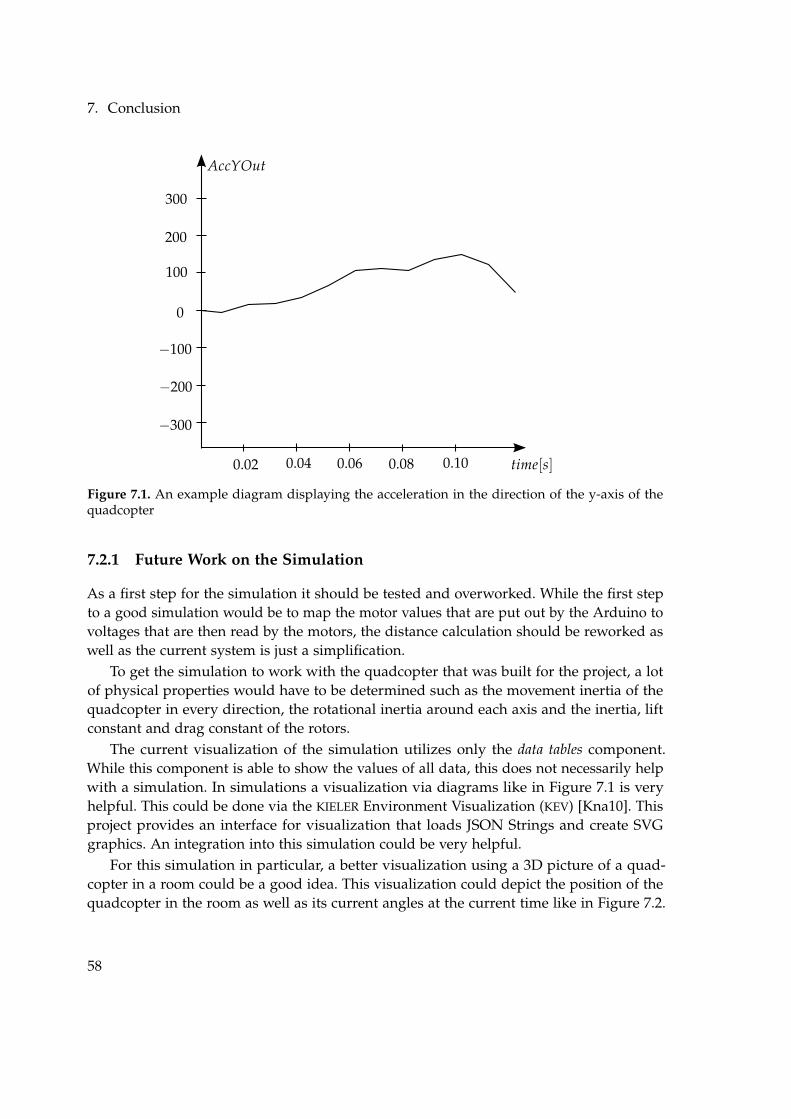
7. Conclusion

AccYOut

time[s]0.02 0.04 0.06 0.08 0.10

0

´100

´200

´300

100

200

300

Figure 7.1. An example diagram displaying the acceleration in the direction of the y-axis of thequadcopter

7.2.1 Future Work on the Simulation

As a first step for the simulation it should be tested and overworked. While the first stepto a good simulation would be to map the motor values that are put out by the Arduino tovoltages that are then read by the motors, the distance calculation should be reworked aswell as the current system is just a simplification.

To get the simulation to work with the quadcopter that was built for the project, a lotof physical properties would have to be determined such as the movement inertia of thequadcopter in every direction, the rotational inertia around each axis and the inertia, liftconstant and drag constant of the rotors.

The current visualization of the simulation utilizes only the data tables component.While this component is able to show the values of all data, this does not necessarily helpwith a simulation. In simulations a visualization via diagrams like in Figure 7.1 is veryhelpful. This could be done via the KIELER Environment Visualization (KEV) [Kna10]. Thisproject provides an interface for visualization that loads JSON Strings and create SVGgraphics. An integration into this simulation could be very helpful.

For this simulation in particular, a better visualization using a 3D picture of a quad-copter in a room could be a good idea. This visualization could depict the position of thequadcopter in the room as well as its current angles at the current time like in Figure 7.2.

58

7.2. Future Work

Figure 7.2. A three-dimensional representation of the quadcopter slightly tilted in a room

The simulation could further give information if the value of a variable has exceeded acertain limit, for example if the quadcopter has exited the boundaries of the room or istilted more then desired. The creator should however analyze the costs and benefits of thiswork. As long as the simulation is not working properly, this visualization would not bevery helpful.

7.2.2 Future Work on Data-Flow

Data-flow in SCCharts has a lot of room for expansion. Since the model with all theequations was already created beforehand, the model was very easy to implement inSCCharts. But, as mentioned in Section 6.3.2, there still exist some issues that need to befixed.

The first step to making data-flow in SCCharts more usable is to improve the layoutalgorithm or to create a way to influence the layout more easily. Right now, unrelatedvariables can be located very close to each other while related ones are very far fromeach other away, which makes it hard to understand the model for outsiders. Even I asthe modeler often times had problems understanding the flow of data in some models.Removing unnecessary markings as well as making it possible to group related variableswithout losing the connection to other variables would be a first step to better layouts. As anexample, Ptolemy does an excellent job providing means to hide unnecessary informationas well as to show connections via the ports of composite models. Data-flow in SCChartsalready does the latter when using nested SCCharts but still struggles with mid-sizedmodels. These models often struggle with unnecessary markings. Removing a marking

59

7. Conclusion

when it is not declared as an input or output variable of the diagram might be a goodidea. Ptolemy handles this fairly well by only portraying the names of ports when the userhovers over this port. This or hovering over the connection to reveal the name instead ofjust the port could be implemented in SCCharts.

Furthermore, trigonometric functions and ways to integrate or derivate are oftentimes very important for physical simulations, which is an important use case for data-flow. Therefore these functions should be more easily accessible. Since trigonometricfunctions are currently merely implemented via the use of hostcode, which in itself is quiteproblematic as the modeler might want a platform independent model, and integration andderivation are not implemented at all, SCCharts clearly lacks a lot of appeal. Implementingthese kinds of functionalities though should not be hard to do. Furthermore, hostcode isnot visualized in data-flow currently. Perhaps creating a small box signifying hostcode inthe diagram could fix this. The hostcode could be written inside the box so the modelerknows what it does instead of it being a black box.

Lastly, Data-flow in SCCharts requires more demonstrators. At this point in time,data-flow in SCCharts has not been used by many people. A larger test – maybe as a partof a course – would be required to verify data-flow and to search for more flaws in theimplementation or the visualization. An important part of this would be to let the studentscreate both smaller and larger models and to conduct a survey afterwards.

In conclusion, this thesis describes with the help of a simulation for a quadcoptera demonstrator for data-flow in SCCharts. With this demonstrator the thesis comparesPtolemy and SCCharts as modeling and simulation tools. It shows the strength andweaknesses of SCCharts in the context of physical simulations.

60

Bibliography

[And15] Lewe Andersen. “‘Quadrocopter Flight-Control Design using SCCharts’”.submitted. Bachelor Thesis. Kiel University, Sept. 2015.

[And96] Charles André. SyncCharts: A Visual Representation of Reactive Behaviors.Tech. rep. RR 95–52, rev. RR 96–56. Sophia-Antipolis, France: I3S, Rev. April1996.

[BB91] Albert Benveniste and Gerard Berry. “The synchronous approach to reactiveand real-time systems”. In: Proceedings of the IEEE. 1991, pp. 1270–1282.

[BCE+03] Albert Benveniste, Paul Caspi, Stephen A. Edwards, Nicolas Halbwachs, PaulLe Guernic, and Robert de Simone. “The Synchronous Languages TwelveYears Later”. In: Proc. IEEE, Special Issue on Embedded Systems. Vol. 91. Piscat-away, NJ, USA: IEEE, Jan. 2003, pp. 64–83.

[CLD05] Pedro Castillo, Rogelio Lozano, and Alejandro Dzul. “Stabilization of a minirotorcraft with four rotors”. In: IEEE Control Systems Magazine 25.6 (2005),pp. 45–55.

[CPP05] Jean-Louis Colaço, Bruno Pagano, and Marc Pouzet. “A conservative exten-sion of synchronous data-flow with state machines”. In: Proceedings of the 5thACM International Conference on Embedded Software. EMSOFT ’05. Jersey City,NJ, USA: ACM, 2005, pp. 173–182. isbn: 1-59593-091-4. doi: 10.1145/1086228.1086261.url: http://doi.acm.org/10.1145/1086228.1086261.

[Gol80] Herbert Goldstein. Classical Mechanics. Addison-Wesley, 1980.

[Hah02] Hubert Hahn. Rigid Body Dynamics of Mechanisms: 1 Theoretical Basics.Springer Science & Business Media, 2002.

[Har87] David Harel. “Statecharts: A visual formalism for complex systems”. In:Science of Computer Programming 8.3 (June 1987), pp. 231–274.

[HDM+14] Reinhard von Hanxleden, Björn Duderstadt, Christian Motika, Steven Smyth,Michael Mendler, Joaquín Aguado, Stephen Mercer, and Owen O’Brien. “SC-Charts: Sequentially Constructive Statecharts for safety-critical applications”.In: Proc. ACM SIGPLAN Conference on Programming Language Design and Imple-mentation (PLDI’14). Edinburgh, UK: ACM, June 2014.

61

Bibliography

[HMA+13] Reinhard von Hanxleden, Michael Mendler, Joaquín Aguado, Björn Duder-stadt, Insa Fuhrmann, Christian Motika, Stephen Mercer, and Owen O’Brien.“Sequentially Constructive Concurrency—A conservative extension of thesynchronous model of computation”. In: Proc. Design, Automation and Test inEurope Conference (DATE’13). Grenoble, France: IEEE, Mar. 2013, pp. 581–586.

[Hög14] Matthias Höger. “‘Aspekte der mathematischen Modellierung eines Quad-copters’”. http : / / num . math . uni - bayreuth . de / de / thesis / 2014 / Hoeger _ Matthias / BA _

Matthias_Hoeger.pdf. bachelor Thesis. University Bayreuth, Sept. 2014.

[Kna10] Stephan Knauer. “‘KEV – KIELER Environment Visualization – Beschreibungeiner Zuordnung von Simulationsdaten und SVG-Graphiken’”. http://rtsys.informatik . uni - kiel . de / ~biblio / downloads / theses / skn - st . pdf. Student researchproject. Kiel University, Department of Computer Science, July 2010.

[Lee03] Edward A. Lee. Overview of the Ptolemy Project. Technical MemorandumUCB/ERL M03/25. University of California, Berkeley, CA, 94720, USA, July2003.

[Lee06] Edward A. Lee. “The problem with threads”. In: IEEE Computer 39.5 (2006),pp. 33–42.

[Luu11] Teppo Luukkonen. “‘Modelling and control of quadcopter’”. http://sal.aalto.fi/publications/pdf-files/eluu11_public.pdf. Bachelor Thesis. Aalto University,Aug. 2011.

[Mac15] Felix Machaczek. “‘Collision Avoidance of Autonomous Safety-Critical Real-Time Systems’”. submitted. Bachelor Thesis. Kiel University, Sept. 2015.

[Mot07] Christian Motika. “‘Modellbasierte Umgebungssimulation für verteilte Echtzeit-systeme mit flexiblem Schnittstellenkonzept’”. http://rtsys.informatik.uni-

kiel.de/~biblio/downloads/theses/cmot-st.pdf. Student research project. Kiel Uni-versity, Department of Computer Science, Oct. 2007.

[Mot09] Christian Motika. “‘Semantics and Execution of Domain Specific Models—KlePto and an Execution Framework’”. http://rtsys.informatik.uni- kiel.de/

~biblio/downloads/theses/cmot-dt.pdf. Diploma thesis. Kiel University, Departmentof Computer Science, Dec. 2009.

[Pto14] Claudius Ptolemaeus, ed. System Design, Modeling, and Simulation usingPtolemy II. http://ptolemy.org/books/Systems. Ptolemy.org, 2014.

[SG78] G. E. Shilov and B. L. Gurevich. Integral, Measure, and Derivative: A UnifiedApproach. Trans. by Richard A. Silverman. Dover Publications, 1978.

62

Bibliography

[SSH14] Christoph Daniel Schulze, Miro Spönemann, and Reinhard von Hanxleden.“Drawing layered graphs with port constraints”. In: Journal of Visual Languagesand Computing, Special Issue on Diagram Aesthetics and Layout 25.2 (2014), pp. 89–106. issn: 1045-926X. doi: 10.1016/j.jvlc.2013.11.005.

[TF96] George B Jr. Thomas and Roos L. Finney. Calculus and Analytic Geometry(9th ed.) Addison-Wesley, 1996.

[TM04] A Tayebi and S McGilvray. “Attitude stabilization of a four-rotor aerial robot”.In: Decision and Control, 2004. CDC. 43rd IEEE Conference on. Vol. 2. IEEE. 2004,pp. 1216–1221.

[Uml15] Axel Umland. “‘Konzept zur Erweiterung von SCCharts um Datenfluss’”.http://rtsys.informatik.uni-kiel.de/~biblio/downloads/theses/aum-dt.pdf. Diplomathesis. Kiel University, Department of Computer Science, Mar. 2015.

63

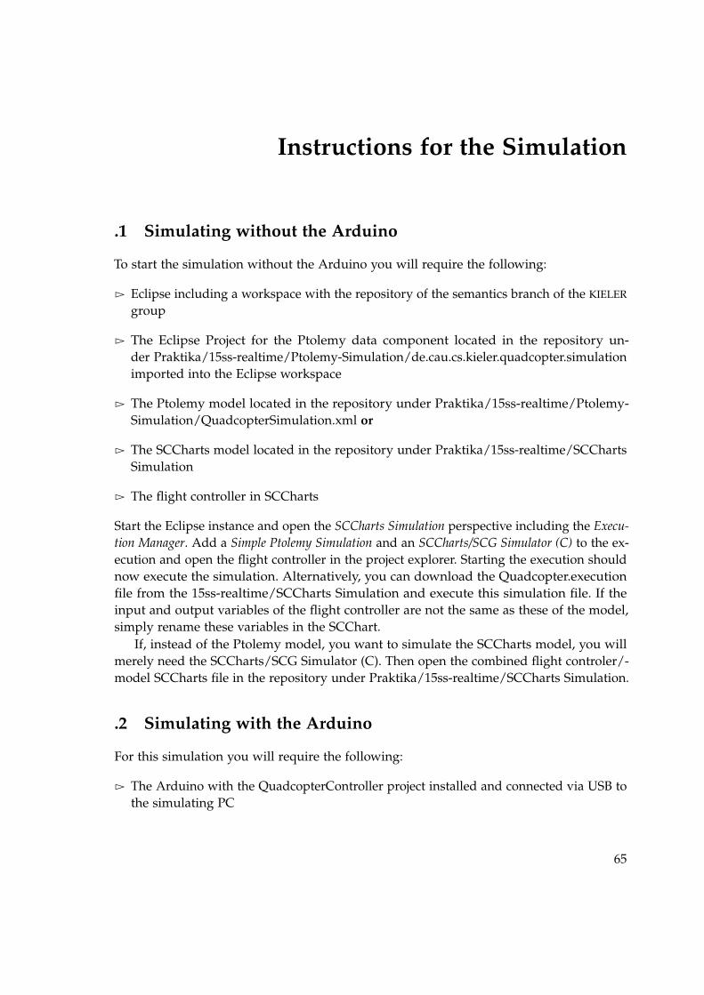
Instructions for the Simulation

.1 Simulating without the Arduino

To start the simulation without the Arduino you will require the following:

Ź Eclipse including a workspace with the repository of the semantics branch of the KIELER

group

Ź The Eclipse Project for the Ptolemy data component located in the repository un-der Praktika/15ss-realtime/Ptolemy-Simulation/de.cau.cs.kieler.quadcopter.simulationimported into the Eclipse workspace

Ź The Ptolemy model located in the repository under Praktika/15ss-realtime/Ptolemy-Simulation/QuadcopterSimulation.xml or

Ź The SCCharts model located in the repository under Praktika/15ss-realtime/SCChartsSimulation

Ź The flight controller in SCCharts

Start the Eclipse instance and open the SCCharts Simulation perspective including the Execu-tion Manager. Add a Simple Ptolemy Simulation and an SCCharts/SCG Simulator (C) to the ex-ecution and open the flight controller in the project explorer. Starting the execution shouldnow execute the simulation. Alternatively, you can download the Quadcopter.executionfile from the 15ss-realtime/SCCharts Simulation and execute this simulation file. If theinput and output variables of the flight controller are not the same as these of the model,simply rename these variables in the SCChart.

If, instead of the Ptolemy model, you want to simulate the SCCharts model, you willmerely need the SCCharts/SCG Simulator (C). Then open the combined flight controler/-model SCCharts file in the repository under Praktika/15ss-realtime/SCCharts Simulation.

.2 Simulating with the Arduino

For this simulation you will require the following:

Ź The Arduino with the QuadcopterController project installed and connected via USB tothe simulating PC

65

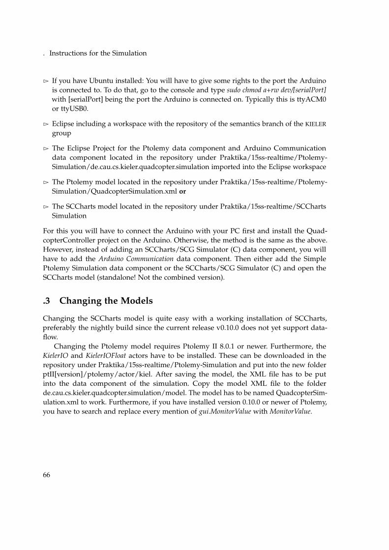
. Instructions for the Simulation

Ź If you have Ubuntu installed: You will have to give some rights to the port the Arduinois connected to. To do that, go to the console and type sudo chmod a+rw dev/[serialPort]with [serialPort] being the port the Arduino is connected on. Typically this is ttyACM0or ttyUSB0.

Ź Eclipse including a workspace with the repository of the semantics branch of the KIELER

group

Ź The Eclipse Project for the Ptolemy data component and Arduino Communicationdata component located in the repository under Praktika/15ss-realtime/Ptolemy-Simulation/de.cau.cs.kieler.quadcopter.simulation imported into the Eclipse workspace

Ź The Ptolemy model located in the repository under Praktika/15ss-realtime/Ptolemy-Simulation/QuadcopterSimulation.xml or

Ź The SCCharts model located in the repository under Praktika/15ss-realtime/SCChartsSimulation

For this you will have to connect the Arduino with your PC first and install the Quad-copterController project on the Arduino. Otherwise, the method is the same as the above.However, instead of adding an SCCharts/SCG Simulator (C) data component, you willhave to add the Arduino Communication data component. Then either add the SimplePtolemy Simulation data component or the SCCharts/SCG Simulator (C) and open theSCCharts model (standalone! Not the combined version).

.3 Changing the Models

Changing the SCCharts model is quite easy with a working installation of SCCharts,preferably the nightly build since the current release v0.10.0 does not yet support data-flow.

Changing the Ptolemy model requires Ptolemy II 8.0.1 or newer. Furthermore, theKielerIO and KielerIOFloat actors have to be installed. These can be downloaded in therepository under Praktika/15ss-realtime/Ptolemy-Simulation and put into the new folderptII[version]/ptolemy/actor/kiel. After saving the model, the XML file has to be putinto the data component of the simulation. Copy the model XML file to the folderde.cau.cs.kieler.quadcopter.simulation/model. The model has to be named QuadcopterSim-ulation.xml to work. Furthermore, if you have installed version 0.10.0 or newer of Ptolemy,you have to search and replace every mention of gui.MonitorValue with MonitorValue.

66