Modelling the Directionality of Light Scattered inTranslucent Materials

Jeppe Revall Frisvad

Joint work withToshiya Hachisuka, Aarhus University

Thomas Kjeldsen, The Alexandra Institute

March 2014

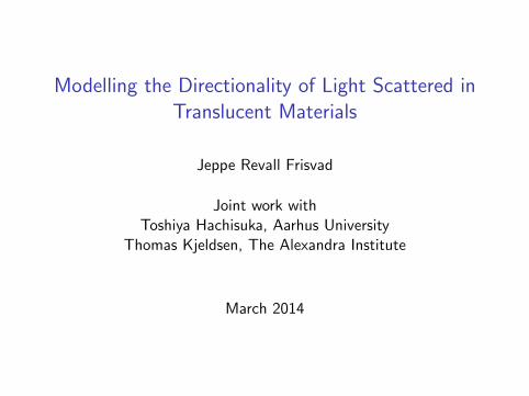
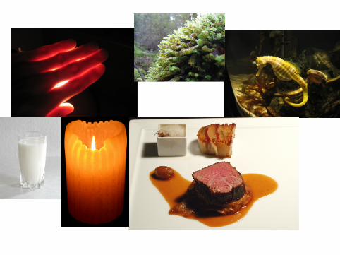
Materials (scattering and absorption of light)

I Optical properties (index of refraction, n(λ) = n′(λ) + i n′′(λ)).

I Reflectance distribution functions, S(xi , ~ωi ; xo , ~ωo).

xi xo

n1

n2

BSSRDF

n1

n2

BRDF

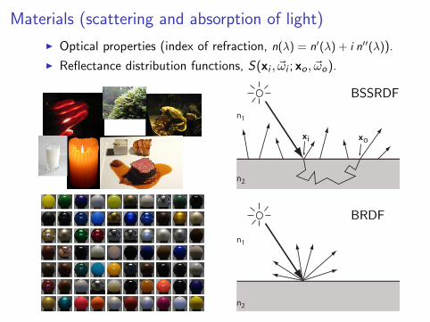
Subsurface scattering

I Behind the rendering equation [Nicodemus et al. 1977]:

dLr (xo , ~ωo)

dΦi (xi , ~ωi )= S(xi , ~ωi ; xo , ~ωo) . xi xo

n1

n2

I An element of reflected radiance dLr is proportional to anelement of incident flux dΦi .

I S (the BSSRDF) is the factor of proportionality.

I Using the definition of radiance L =d2Φ

cos θ dA dω, we have

Lr (xo , ~ωo) =

∫

A

∫

2πS(xi , ~ωi ; xo , ~ωo)Li (xi , ~ωi ) cos θ dωi dA .

References

- Nicodemus, F. E., Richmond, J. C., Hsia, J. J., Ginsberg, I. W., and Limperis, T. Geometricalconsiderations and nomenclature for reflectance. Tech. rep., National Bureau of Standards (US), 1977.

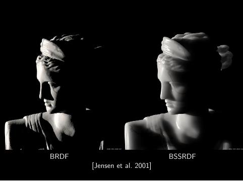
BRDF BSSRDF[Jensen et al. 2001]

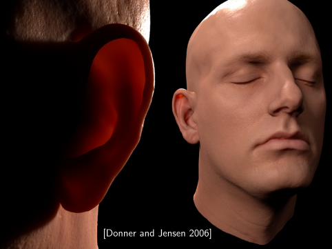
[Donner and Jensen 2006]

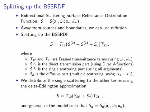
Splitting up the BSSRDF

I Bidirectional Scattering-Surface Reflectance DistributionFunction: S = S(xi , ~ωi ; xo , ~ωo) .

I Away from sources and boundaries, we can use diffusion.

I Splitting up the BSSRDF

S = T12(S (0) + S (1) + Sd)T21 .

whereI T12 and T21 are Fresnel transmittance terms (using ~ωi , ~ωo).I S (0) is the direct transmission part (using Dirac δ-functions).I S (1) is the single scattering part (using all arguments).I Sd is the diffusive part (multiple scattering, using |xo − xi |).

I We distribute the single scattering to the other terms usingthe delta-Eddington approximation:

S = T12(SδE + Sd)T21 ,

and generalize the model such that Sd = Sd(xi , ~ωi ; xo).

Diffusion theory

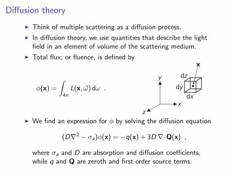
I Think of multiple scattering as a diffusion process.

I In diffusion theory, we use quantities that describe the lightfield in an element of volume of the scattering medium.

I Total flux, or fluence, is defined by

φ(x) =

∫

4πL(x, ~ω) dω .

x

y

z

x

dxdy

dz

I We find an expression for φ by solving the diffusion equation

(D∇2 − σa)φ(x) = −q(x) + 3D∇·Q(x) ,

where σa and D are absorption and diffusion coefficients,while q and Q are zeroth and first order source terms.

Deriving a BSSRDF

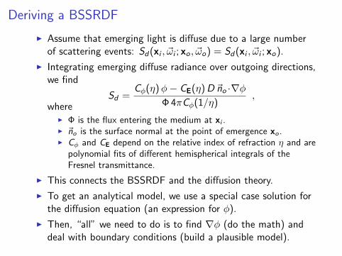
I Assume that emerging light is diffuse due to a large numberof scattering events: Sd(xi , ~ωi ; xo , ~ωo) = Sd(xi , ~ωi ; xo).

I Integrating emerging diffuse radiance over outgoing directions,we find

Sd =Cφ(η)φ− CE(η)D ~no ·∇φ

Φ 4πCφ(1/η),

whereI Φ is the flux entering the medium at xi .I ~no is the surface normal at the point of emergence xo .I Cφ and CE depend on the relative index of refraction η and are

polynomial fits of different hemispherical integrals of theFresnel transmittance.

I This connects the BSSRDF and the diffusion theory.

I To get an analytical model, we use a special case solution forthe diffusion equation (an expression for φ).

I Then, “all” we need to do is to find ∇φ (do the math) anddeal with boundary conditions (build a plausible model).

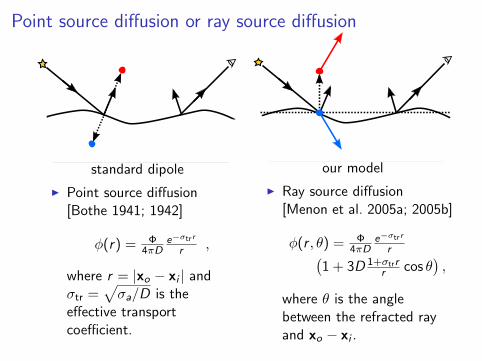
Point source diffusion or ray source diffusion

standard dipole

I Point source diffusion[Bothe 1941; 1942]

φ(r) = Φ4πD

e−σtrr

r ,

where r = |xo − xi | andσtr =

√σa/D is the

effective transportcoefficient.

our model

I Ray source diffusion[Menon et al. 2005a; 2005b]

φ(r , θ) = Φ4πD

e−σtrr

r(1 + 3D 1+σtrr

r cos θ),

where θ is the anglebetween the refracted rayand xo − xi .

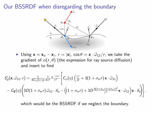
Our BSSRDF when disregarding the boundary

d

I Using x = xo − xi , r = |x|, cos θ = x · ~ω12/r , we take thegradient of φ(r , θ) (the expression for ray source diffusion)and insert to find

S ′d(x, ~ω12, r) = 1

4Cφ(1/η)1

4π2e−σtrr

r3

[Cφ(η)

(r2

D + 3(1 + σtrr) x · ~ω12

)

− CE(η)

(3D(1 + σtrr) ~ω12 · ~no −

((1 + σtrr) + 3D 3(1+σtrr)+(σtrr)2

r2 x · ~ω12

)x · ~no

)],

which would be the BSSRDF if we neglect the boundary.

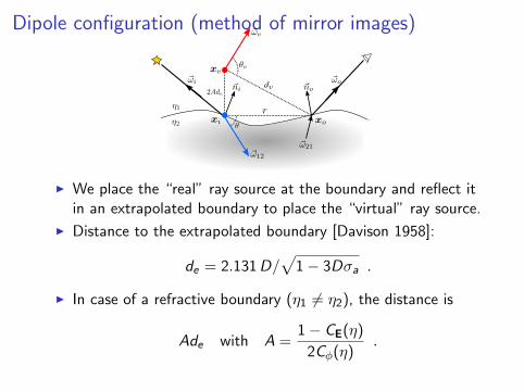
Dipole configuration (method of mirror images)

d

I We place the “real” ray source at the boundary and reflect itin an extrapolated boundary to place the “virtual” ray source.

I Distance to the extrapolated boundary [Davison 1958]:

de = 2.131D/√

1− 3Dσa .

I In case of a refractive boundary (η1 6= η2), the distance is

Ade with A =1− CE(η)

2Cφ(η).

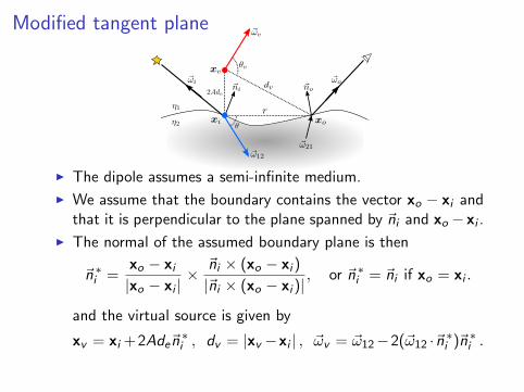
Modified tangent plane

d

I The dipole assumes a semi-infinite medium.

I We assume that the boundary contains the vector xo − xi andthat it is perpendicular to the plane spanned by ~ni and xo − xi .

I The normal of the assumed boundary plane is then

~n ∗i =xo − xi|xo − xi |

× ~ni × (xo − xi )

|~ni × (xo − xi )|, or ~n ∗i = ~ni if xo = xi .

and the virtual source is given by

xv = xi + 2Ade~n∗i , dv = |xv −xi | , ~ωv = ~ω12−2(~ω12 ·~n ∗i )~n ∗i .

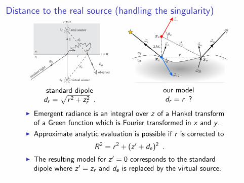
Distance to the real source (handling the singularity)

r

z-axis

z

-zv

r

ωi ωo

n

dv

z = 0

dr

real source

virtual source

observerincid

ent light

n2

n1

standard dipoledr =

√r2 + z2

r .

d

our modeldr = r ?

I Emergent radiance is an integral over z of a Hankel transformof a Green function which is Fourier transformed in x and y .

I Approximate analytic evaluation is possible if r is corrected to

R2 = r2 + (z ′ + de)2 .

I The resulting model for z ′ = 0 corresponds to the standarddipole where z ′ = zr and de is replaced by the virtual source.

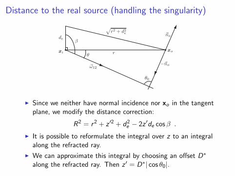
Distance to the real source (handling the singularity)

√r2 + d2e

de

xixo

�ω12

θ

θ0

�no

−�no

r

β

I Since we neither have normal incidence nor xo in the tangentplane, we modify the distance correction:

R2 = r2 + z ′2 + d2e − 2z ′de cosβ .

I It is possible to reformulate the integral over z to an integralalong the refracted ray.

I We can approximate this integral by choosing an offset D∗

along the refracted ray. Then z ′ = D∗| cos θ0|.

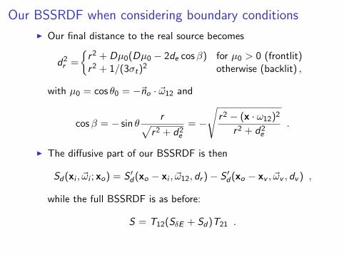
Our BSSRDF when considering boundary conditions

I Our final distance to the real source becomes

d2r =

{r2 + Dµ0(Dµ0 − 2de cosβ) for µ0 > 0 (frontlit)r2 + 1/(3σt)

2 otherwise (backlit) ,

with µ0 = cos θ0 = −~no · ~ω12 and

cosβ = − sin θr√

r2 + d2e

= −√

r2 − (x · ω12)2

r2 + d2e

.

I The diffusive part of our BSSRDF is then

Sd(xi , ~ωi ; xo) = S ′d(xo − xi , ~ω12, dr )− S ′d(xo − xv , ~ωv , dv ) ,

while the full BSSRDF is as before:

S = T12(SδE + Sd)T21 .

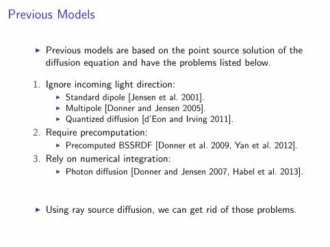
Previous Models

I Previous models are based on the point source solution of thediffusion equation and have the problems listed below.

1. Ignore incoming light direction:I Standard dipole [Jensen et al. 2001].I Multipole [Donner and Jensen 2005].I Quantized diffusion [d’Eon and Irving 2011].

2. Require precomputation:I Precomputed BSSRDF [Donner et al. 2009, Yan et al. 2012].

3. Rely on numerical integration:I Photon diffusion [Donner and Jensen 2007, Habel et al. 2013].

I Using ray source diffusion, we can get rid of those problems.

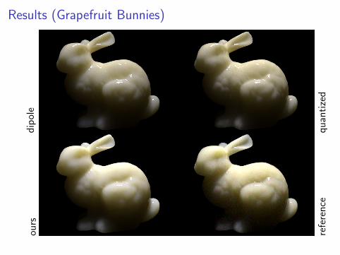
Results (Grapefruit Bunnies)d

ipol

e

qu

anti

zed

ours

refe

ren

ce

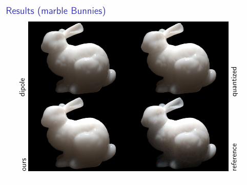
Results (marble Bunnies)d

ipol

e

qu

anti

zed

ours

refe

ren

ce

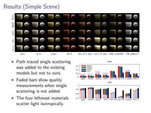
Results (Simple Scene)

I Path traced single scatteringwas added to the existingmodels but not to ours.

I Faded bars show qualitymeasurements when singlescattering is not added.

I The four leftmost materialsscatter light isotropically.

0

0.1

0.2

0.3

RMSE

apple marble potato skin1 choc milk soy milk w. grape milk (r.)

dipolebtpoleqntzdours

0.7

0.8

0.9

1

SSIM

apple marble potato skin1 choc milk soy milk w. grape milk (r.)

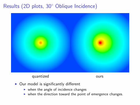
Results (2D plots, 30◦ Oblique Incidence)

quantized ours

I Our model is significantly differentI when the angle of incidence changesI when the direction toward the point of emergence changes.

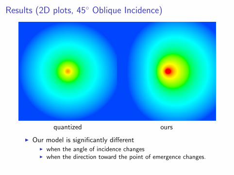
Results (2D plots, 45◦ Oblique Incidence)

quantized ours

I Our model is significantly differentI when the angle of incidence changesI when the direction toward the point of emergence changes.

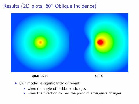
Results (2D plots, 60◦ Oblique Incidence)

quantized ours

I Our model is significantly differentI when the angle of incidence changesI when the direction toward the point of emergence changes.

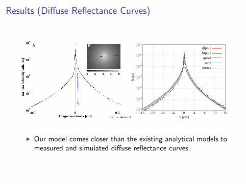
Results (Diffuse Reflectance Curves)

R (

x)d

-16 -12 -8 -4 0 4 8 12 16

10 1

10 0

10 -1

10 -2

10 -3

10 -4

10 -5

dipolebtpoleqntzdours

ptrace

dipolebtpoleqntzdours

ptrace

I Our model comes closer than the existing analytical models tomeasured and simulated diffuse reflectance curves.

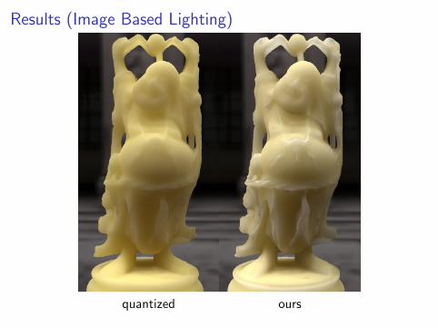
Results (Image Based Lighting)

quantized ours

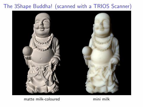
The 3Shape Buddha! (scanned with a TRIOS Scanner)

matte milk-coloured mini milk

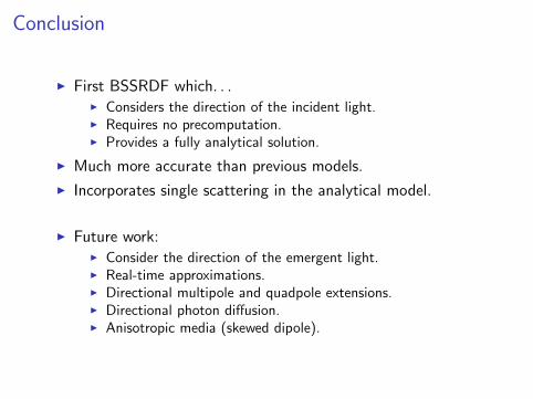
Conclusion

I First BSSRDF which. . .I Considers the direction of the incident light.I Requires no precomputation.I Provides a fully analytical solution.

I Much more accurate than previous models.

I Incorporates single scattering in the analytical model.

I Future work:I Consider the direction of the emergent light.I Real-time approximations.I Directional multipole and quadpole extensions.I Directional photon diffusion.I Anisotropic media (skewed dipole).