Embed Size (px)
Citation preview
Modelos Híbridos de Deslocamentos para a Análise
Fisicamente não Linear de Estruturas Tridimensionais de Betão
João Miguel de Oliveira Durães Alves Martins
Dissertação para a obtenção do Grau de Mestre em
Engenharia Civil
Júri
Presidente: Professor Pedro Guilherme Sampaio Viola Parreira
Orientador: Professor Luís Manuel Soares dos Santos Castro
Co-Orientador: Professor Eduardo Manuel Baptista Ribeiro Pereira
Vogal: Professora Maria Cristina de Oliveira Matos Silva
Outubro de 2009

At all stages of the development of numerical methodology by engineers,
the achievement of practical results is paramount.
O. C. Zienkiewicz, in The Era of Computational Mechanics: Where Do We Go Now (2001)


i
Acknowledgement
When I was given the opportunity of joining this project on the development of damage and
fracture models for concrete structures based on hybrid and mixed finite elements, I could hardly
imagine how much my life would change and how much I would grow up during this one and a half
years. Even if much of what I earned is not directly related to this work, this period was marked by
extraordinary people I met and worked with, new friends that made all the difference, big
opportunities that were suddenly open to me as well as daring perspectives that I had not seen
before and, undoubtedly, this dissertation is the paramount achievement of this period.
First of all, I want to thank the people who accompanied me during this work, especially
Professor Luis Castro. Along this dissertation, he was an extraordinarily eager and attentive
supervisor. However, more than a supervisor, he was a professor; more than a professor, he was a
teacher and more than teacher, he was a friend. That is something I will never forget.
I also thank Professor Eduardo Pereira for all the eagerness in causing exponential softening to
my already damaged brain when the time came to introduce me to non-conventional finite element
formulations.
I want to thank my colleague, Carla Garrido. We found in each other great support and learned
how to have a laugh at the ups and downs of a research process and how to cooperate so that each
of us could give their best in this project. Moreover, days at Técnico would not be the same without
Mário Arruda, who helped me in many ways with his great advices and good mood, his personal
views on engineering and his keen and critical opinions.
I want to thank Fundação para a Ciência e Tecnologia (PTDC/ECM/71519/2006) for the financial
support, which is, in fact, a great incitement to give the first steps in the demanding work of scientific
investigation.
The theoretical part of the dissertation was greatly enriched by the available documents at the
Technische Universiteit Delft. I am very grateful for having had the opportunity of being an exchange
student at such a great university. Erasmus opened my eyes to new philosophies of teaching,
different perspectives on academic objectives, as well as widening my horizons to other cultures and
other places. I cannot help but thank everyone that jazzed up these wonderful, unforgettable and
unrepeatable months, all the incredible friends that are the best thing I take from this great Erasmus
experience.

ii
I am also very grateful to all my friends. Life teaches us that human relationships are demanding
and so one should choose one’s friends wisely. I am glad that time has showed me that I know
extraordinary people who cheer me up when I am down, give me good advice when I am confused
and help me when I feel exhausted. These are the friends who, in the end, made all the special
moments of my life truly special.
Undeniably, these acknowledgements and anything I can ever write will never repay all the love,
all the attention and all the precious lessons my parents gave me. Nevertheless, I hope they feel their
reward in my achievements and in my everyday posture as much as I feel grateful and privileged for
their unconditional support. I also owe my grandparents a huge debt of gratitude, and these
recognitions would be incomplete without this sign that I will never forget them or disregard their
huge contribution to who I am and how far I have come. I know this work would make them very
proud of me as this is not only my accomplishment but also theirs.
Finally, I find it appropriate to thank the one who said that the first should be the last. He knows
better than anyone how much this period of my life meant to me and how much I evolved during it,
for He was always with me and, ultimately, I thank it all to Him. As I have no better words to write
than those that are not my own, I conclude these acknowledgements with the last stanza of my
favourite poem:
E eu vou, e a luz do gládio erguido dá
Em minha face calma.
Cheio de Deus, não temo o que virá,
Pois, venha o que vier, nunca será
Maior que a minha alma.
Fernando Pessoa, in Mensagem
iii
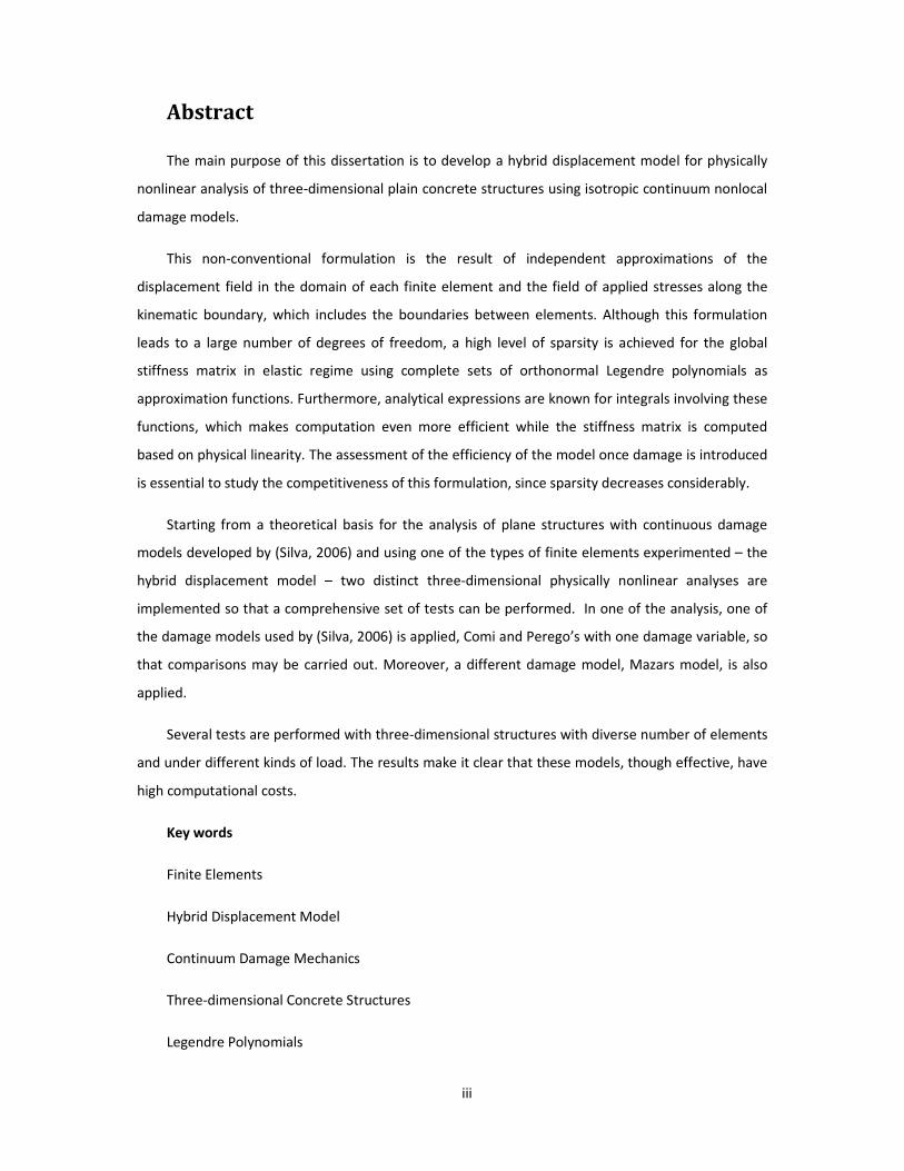
Abstract
The main purpose of this dissertation is to develop a hybrid displacement model for physically
nonlinear analysis of three-dimensional plain concrete structures using isotropic continuum nonlocal
damage models.
This non-conventional formulation is the result of independent approximations of the
displacement field in the domain of each finite element and the field of applied stresses along the
kinematic boundary, which includes the boundaries between elements. Although this formulation
leads to a large number of degrees of freedom, a high level of sparsity is achieved for the global
stiffness matrix in elastic regime using complete sets of orthonormal Legendre polynomials as
approximation functions. Furthermore, analytical expressions are known for integrals involving these
functions, which makes computation even more efficient while the stiffness matrix is computed
based on physical linearity. The assessment of the efficiency of the model once damage is introduced
is essential to study the competitiveness of this formulation, since sparsity decreases considerably.
Starting from a theoretical basis for the analysis of plane structures with continuous damage
models developed by (Silva, 2006) and using one of the types of finite elements experimented – the
hybrid displacement model – two distinct three-dimensional physically nonlinear analyses are
implemented so that a comprehensive set of tests can be performed. In one of the analysis, one of
the damage models used by (Silva, 2006) is applied, Comi and Perego’s with one damage variable, so
that comparisons may be carried out. Moreover, a different damage model, Mazars model, is also
applied.
Several tests are performed with three-dimensional structures with diverse number of elements
and under different kinds of load. The results make it clear that these models, though effective, have
high computational costs.
Key words
Finite Elements
Hybrid Displacement Model
Continuum Damage Mechanics
Three-dimensional Concrete Structures
Legendre Polynomials

iv
v
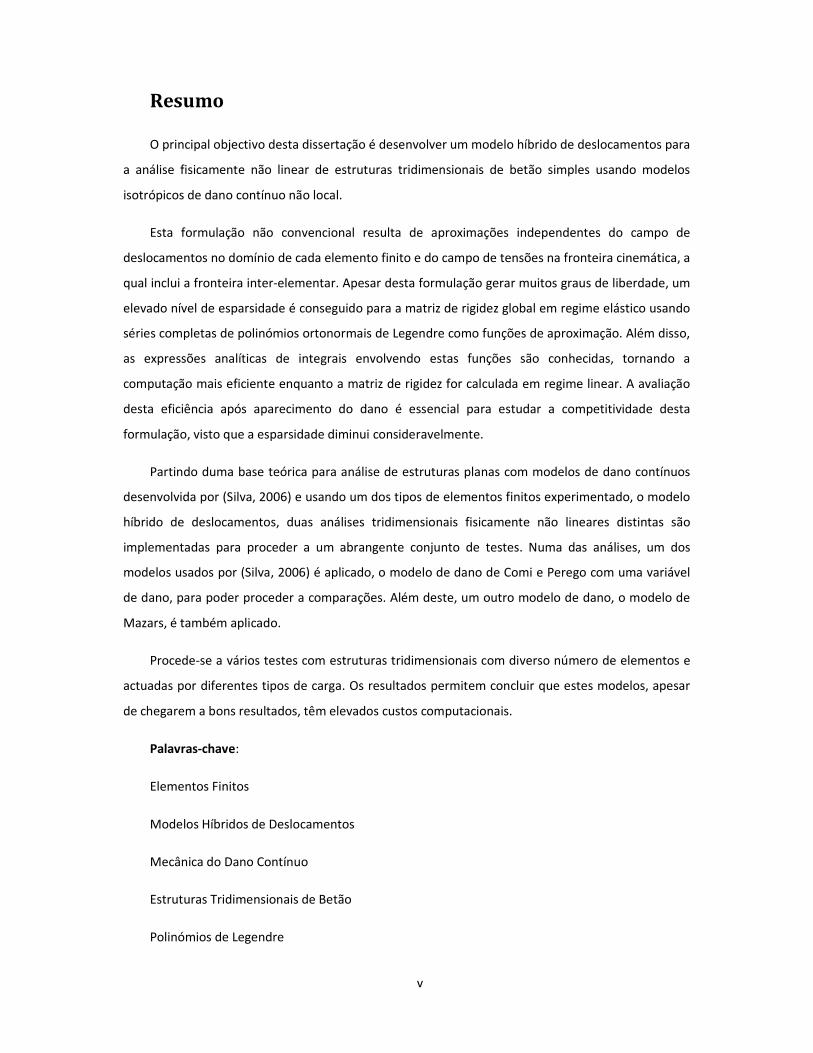
Resumo
O principal objectivo desta dissertação é desenvolver um modelo híbrido de deslocamentos para
a análise fisicamente não linear de estruturas tridimensionais de betão simples usando modelos
isotrópicos de dano contínuo não local.
Esta formulação não convencional resulta de aproximações independentes do campo de
deslocamentos no domínio de cada elemento finito e do campo de tensões na fronteira cinemática, a
qual inclui a fronteira inter-elementar. Apesar desta formulação gerar muitos graus de liberdade, um
elevado nível de esparsidade é conseguido para a matriz de rigidez global em regime elástico usando
séries completas de polinómios ortonormais de Legendre como funções de aproximação. Além disso,
as expressões analíticas de integrais envolvendo estas funções são conhecidas, tornando a
computação mais eficiente enquanto a matriz de rigidez for calculada em regime linear. A avaliação
desta eficiência após aparecimento do dano é essencial para estudar a competitividade desta
formulação, visto que a esparsidade diminui consideravelmente.
Partindo duma base teórica para análise de estruturas planas com modelos de dano contínuos
desenvolvida por (Silva, 2006) e usando um dos tipos de elementos finitos experimentado, o modelo
híbrido de deslocamentos, duas análises tridimensionais fisicamente não lineares distintas são
implementadas para proceder a um abrangente conjunto de testes. Numa das análises, um dos
modelos usados por (Silva, 2006) é aplicado, o modelo de dano de Comi e Perego com uma variável
de dano, para poder proceder a comparações. Além deste, um outro modelo de dano, o modelo de
Mazars, é também aplicado.
Procede-se a vários testes com estruturas tridimensionais com diverso número de elementos e
actuadas por diferentes tipos de carga. Os resultados permitem concluir que estes modelos, apesar
de chegarem a bons resultados, têm elevados custos computacionais.
Palavras-chave:
Elementos Finitos
Modelos Híbridos de Deslocamentos
Mecânica do Dano Contínuo
Estruturas Tridimensionais de Betão
Polinómios de Legendre

vi
vii
Table of Contents
1. Introduction ............................................................................................................................. 1
1.1. General considerations ................................................................................................... 1
1.2. Objectives ........................................................................................................................ 3
1.3. Organization .................................................................................................................... 5
2. Problem formulation................................................................................................................ 7
2.1. Initial considerations ....................................................................................................... 7
2.2. Fundamental equations .................................................................................................. 9
2.2.1. Equilibrium conditions ........................................................................................... 10
2.2.2. Compatibility conditions........................................................................................ 11
2.2.3. Constitutive relationship ....................................................................................... 11
2.3. Concrete behaviour ....................................................................................................... 12
3. Damage models ..................................................................................................................... 17
3.1. Initial considerations ..................................................................................................... 17
3.2. Nature of the phenomenon .......................................................................................... 18
3.3. Comi and Perego’s damage model ................................................................................ 22
3.4. Mazars damage model .................................................................................................. 24
3.5. Comparison of both damage models in uniaxial tensile tests ...................................... 28
3.6. Strain localization and regularization methods ............................................................. 31
4. Finite element formulation .................................................................................................... 35
4.1. Initial considerations ..................................................................................................... 35
4.2. Hybrid displacement model as a non-conventional finite element formulation .......... 36
4.3. Mathematical description of the hybrid displacement model ...................................... 38
5. Computational application .................................................................................................... 41
5.1. Initial considerations ..................................................................................................... 41
5.2. Implementation ............................................................................................................. 42
5.2.1. Approximation functions ....................................................................................... 42
viii
5.2.2. Structure’s geometry ............................................................................................. 43
5.2.3. Structural operators .............................................................................................. 44
5.2.4. Governing system .................................................................................................. 48
5.3. Structure of the program .............................................................................................. 50
6. Numerical tests ...................................................................................................................... 53
6.1. Initial considerations ..................................................................................................... 53
6.2. Analysis of an L-shaped structure ................................................................................. 54
6.3. Analysis of a cantilevered cube under uniform load ..................................................... 63
6.4. Analysis of a cube with imposed displacement ............................................................ 67
6.5. Analysis of a fixed-fixed beam ....................................................................................... 74
6.6. (Hassanzadeh, 1991) test .............................................................................................. 77
7. Conclusions and further developments ................................................................................. 87
7.1. Conclusions .................................................................................................................... 87
7.2. Further developments ................................................................................................... 89
References ..................................................................................................................................... 93
APPENDIXES ................................................................................................................................... 97
Appendix A – Computation of the elastic generalised elemental stiffness operator ............... 98
ix
List of figures
Figure 2.1 – Generic solid ........................................................................................................................ 9
Figure 2.2 – Three-dimensional stress element .................................................................................... 10
Figure 2.3 – Experimental results for stress-strain behaviour under uniaxial loading (Mazars, 1984) 13
Figure 2.4 – Qualitative description of concrete’s behaviour under a uniaxial tension experiment
(Silva, 2006) ........................................................................................................................................... 15
Figure 3.1 – Representative volume element in a damaged solid (Silva, 2006) ................................... 19
Figure 3.2 – Uniaxial damage model using the principle of strain equivalence (Silva, 2006) ............... 20
Figure 3.3 – Modelled results for stress-strain behaviour under uniaxial loading (Proença, 1992) ..... 27
Figure 3.4 – Damage evolution (matching damage models) ................................................................ 29
Figure 3.5 – Stress-strain diagrams (matching damage models) .......................................................... 29
Figure 3.6 – Damage evolution (mismatching damage models) ........................................................... 30
Figure 3.7 – Stress-strain diagrams (mismatching damage models)..................................................... 30
Figure 5.1 – Schematic coordinate transformation in hexahedric elements (Kaltenbacher, 2007) ..... 43
Figure 5.2 – Secant method for solving non-linear equations .............................................................. 49
Figure 6.1 – L-shaped structure with full moment connection and imposed displacement at the tip 54
Figure 6.2 – Matrix of the governing system of the L-shaped structure when nv = 2 and ng = 1 .......... 55
Figure 6.3 – Evolution of damage following Comi and Perego’s model in the L-shaped structure ...... 58
Figure 6.4 – Evolution of damage following Mazars model in the L-shaped structure ........................ 59
Figure 6.5 – Damage in the bisector plane of the L-shaped structure (ū = 1.00 mm) .......................... 59
Figure 6.6 - Effective stress fields in the L-shaped structure in nonlinear analysis (ū = 1.00 mm) ....... 60
Figure 6.7 – Elastic stress diagrams in the L-shaped structure when nv = 4 and ng = 3 ........................ 62
Figure 6.8 – Elastic stress diagrams in the L-shaped structure when nv = 6 and ng = 5 ........................ 62
Figure 6.9 – Elastic stress diagrams in the L-shaped structure when nv = 8 and ng = 7 ........................ 62
Figure 6.10 – Cantilevered cube ............................................................................................................ 64
Figure 6.11 – Elastic stress diagrams in the cantilevered cube (tγγγγ = 1.00 MPa) .................................... 65
Figure 6.12 – Damage in the cantilevered cube (tγγγγ = 2.00 MPa) ........................................................... 65
Figure 6.13 - Relevant effective stress fields in the loaded cube in nonlinear analysis (tγγγγ = 2.0 MPa) . 66
Figure 6.14 – Load-displacement curve for the cantilevered cube ....................................................... 67
Figure 6.15 – Cube with imposed displacement ................................................................................... 68
Figure 6.16 – σyy stress (MPa) in the cube when ū = 0.05 mm (looking at the fixed face) .................. 69
Figure 6.17 – Stress diagrams at plane x = 0.5 m when ū = 0.05 mm ................................................... 69
Figure 6.18 – Damage when ū = 0.1 mm and characteristic length = 0.1 m (looking at the fixed face)70
Figure 6.19 – Damage in the stretched cube following Comi and Perego’s damage model ................ 71
x
Figure 6.20 – Damage in the stretched cube following Mazars damage model ................................... 72
Figure 6.21 – Effective σyy (MPa) for ū = 0.2 mm with Comi and Perego’s model .............................. 73
Figure 6.22 – The fixed-fixed beam ....................................................................................................... 74
Figure 6.23 – σyz (MPa) stresses of the fixed-fixed beam in elastic regime ......................................... 75
Figure 6.24 – σyy (MPa) stresses of the fixed-fixed beam in elastic regime ......................................... 76
Figure 6.25 – Damaged beam for tγγγγ = 500 kN/m2 ................................................................................. 76
Figure 6.26 – Damaged beam for γγγγ = 250 kN/m3 .................................................................................. 76
Figure 6.27 – Geometry of the (Hassanzadeh, 1991) test and coordinate system ............................... 77
Figure 6.28 – Mesh of 19 elements in (Hassanzadeh, 1991) test ......................................................... 78
Figure 6.29 – Mesh of 37 elements in (Hassanzadeh, 1991) test ......................................................... 78
Figure 6.30 – Dimensions of the concrete specimen and finite elements (in cm) ................................ 78
Figure 6.31 – Elastic stress diagrams in plane x=3.50 cm of (Hassanzadeh, 1991) test ........................ 80
Figure 6.32 – Elastic stress diagrams in plane x=3.50 cm of (Hassanzadeh, 1991) test ........................ 81
Figure 6.33 - Damage in the (Hassanzadeh, 1991) test – mesh of 19 elements (ū = 0.004 mm) ......... 82
Figure 6.34 - Damage in the (Hassanzadeh, 1991) test – mesh of 19 elements (ū = 0.010 mm) ......... 82
Figure 6.35 – Damage evolution in (Hassanzadeh, 1991) test (plane x = 3.50 cm) .............................. 83
Figure 6.36 – Numerical results of the load [N] - displacement [mm] curves for the (Hassanzadeh,
1991) test .............................................................................................................................................. 84
Figure 6.37 - Numerical results of the load [N] - displacement [mm] curves for the (Hassanzadeh,
1991) test with 37-element meshes (smoothed curves) ...................................................................... 85
Figure 6.38 – Load [N] - displacement [mm] curves for (Hassanzadeh, 1991) test (adapted from (Silva,
2006)) .................................................................................................................................................... 86
xi
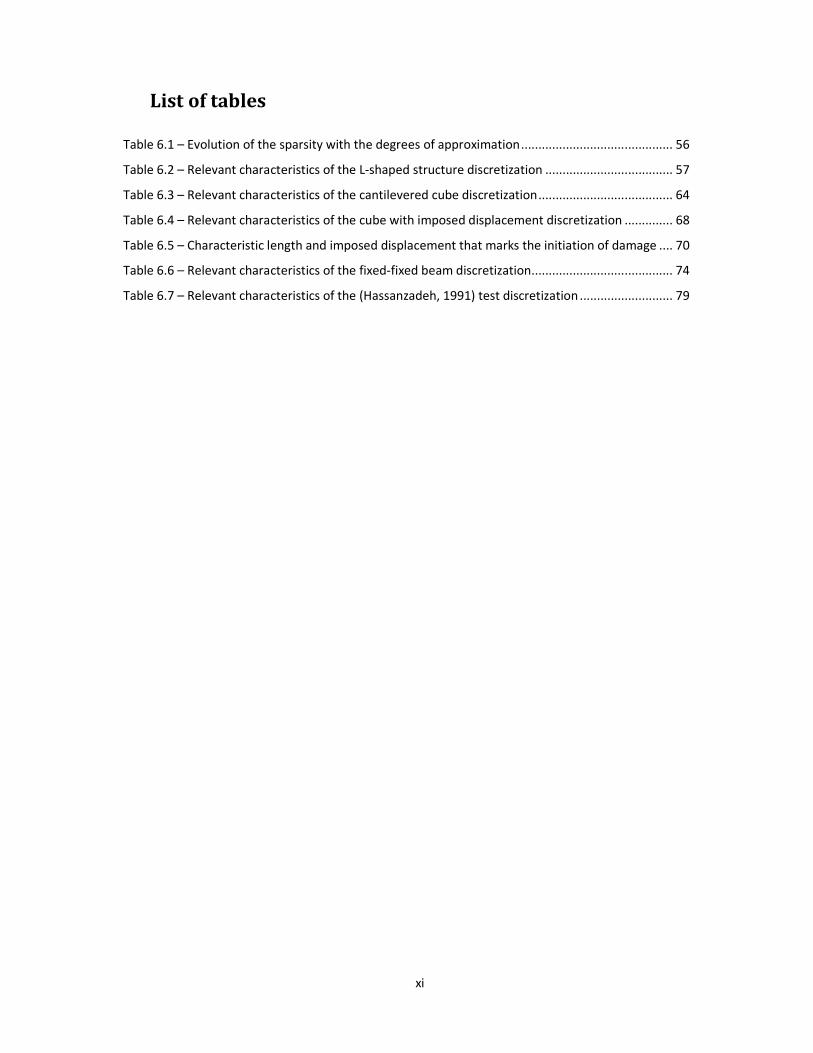
List of tables
Table 6.1 – Evolution of the sparsity with the degrees of approximation ............................................ 56
Table 6.2 – Relevant characteristics of the L-shaped structure discretization ..................................... 57
Table 6.3 – Relevant characteristics of the cantilevered cube discretization ....................................... 64
Table 6.4 – Relevant characteristics of the cube with imposed displacement discretization .............. 68
Table 6.5 – Characteristic length and imposed displacement that marks the initiation of damage .... 70
Table 6.6 – Relevant characteristics of the fixed-fixed beam discretization......................................... 74
Table 6.7 – Relevant characteristics of the (Hassanzadeh, 1991) test discretization ........................... 79

xii
xiii
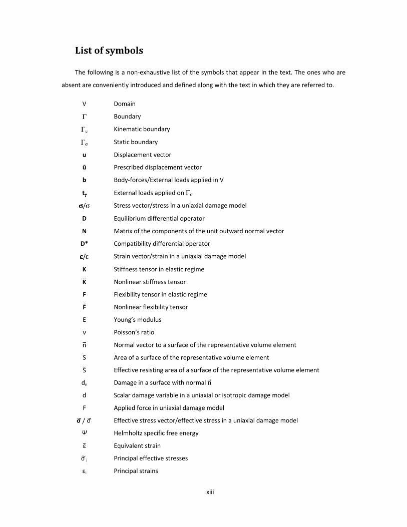
List of symbols
The following is a non-exhaustive list of the symbols that appear in the text. The ones who are
absent are conveniently introduced and defined along with the text in which they are referred to.
V Domain
Γ Boundary
Γu Kinematic boundary
Γσ Static boundary
u Displacement vector
ū Prescribed displacement vector
b Body-forces/External loads applied in V
tγγγγ External loads applied on Γσ
σσσσ/σ Stress vector/stress in a uniaxial damage model
D Equilibrium differential operator
N Matrix of the components of the unit outward normal vector
D* Compatibility differential operator
εεεε/ε Strain vector/strain in a uniaxial damage model
K Stiffness tensor in elastic regime
K� Nonlinear stiffness tensor
F Flexibility tensor in elastic regime
F� Nonlinear flexibility tensor
E Young’s modulus
ν Poisson’s ratio
n�� Normal vector to a surface of the representative volume element
S Area of a surface of the representative volume element
S� Effective resisting area of a surface of the representative volume element
dn Damage in a surface with normal n��
d Scalar damage variable in a uniaxial or isotropic damage model
F Applied force in uniaxial damage model
σ �/ σ �
Ψ
Effective stress vector/effective stress in a uniaxial damage model
Helmholtz specific free energy
ε Equivalent strain
σ � i Principal effective stresses
εi Principal strains
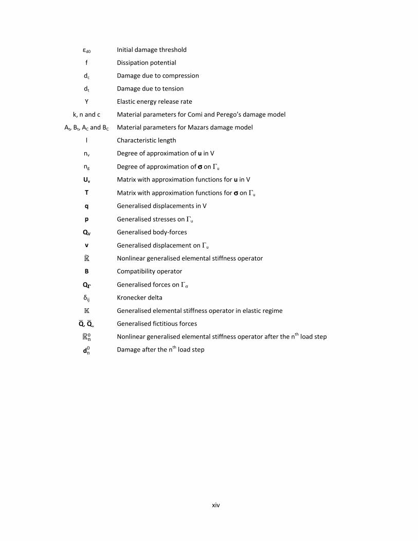
xiv
εd0 Initial damage threshold
f Dissipation potential
dc Damage due to compression
dt Damage due to tension
Y Elastic energy release rate
k, n and c Material parameters for Comi and Perego’s damage model
At, Bt, AC and BC Material parameters for Mazars damage model
l Characteristic length
nv Degree of approximation of u in V
ng Degree of approximation of σσσσ on Γu
Uv Matrix with approximation functions for u in V
T Matrix with approximation functions for σσσσ on Γu
q Generalised displacements in V
p Generalised stresses on Γu
QV Generalised body-forces
v Generalised displacement on Γu � Nonlinear generalised elemental stiffness operator
B Compatibility operator
QΓΓΓΓ Generalised forces on Γσ
δij Kronecker delta Generalised elemental stiffness operator in elastic regime
Q�, Q�∗ Generalised fictitious forces � �� Nonlinear generalised elemental stiffness operator after the nth load step
dn0 Damage after the nth load step
1
1. Introduction
1.1. General considerations
Most of the engineering problems, and Civil Engineering is not an exception, can be expressed
mathematically in terms of differential equations, with or without known analytical solution. The
search for a numerical systematic way of solving these problems led to finite element formulations,
derived from the displacement method, well-known and theoretically established in the structural
analysis framework.
For some decades now, finite element methods have been broadly used to solve continuous
mechanics problems applied to structures with irregular geometries, complicated boundary
conditions and non-homogeneous material properties (Zienkiewicz, 1977). However, the
conventional formulations with conforming displacement elements are limited by the fact that they
return a compatible solution, which is not necessarily in equilibrium with the applied load. In view of
plastic analysis, it is known that if the solution is both compatible and respects equilibrium, it means
that the exact solution was found. In finite element methodology this can only happen if the
approximation functions can generate the exact solution. When problems get more complex, this is
no longer feasible. Furthermore, the compatibility is assured by using compatible approximation
functions, which are proven to get numerically unstable as its degree is increased, therefore
restraining the use of p-refinement strategies. Instead, h-refinements are widely adopted despite the
mesh-generation handicaps. Already back in the 70’s Professor Olgierd Zienkiewicz, one of the
leading researchers of computational mechanics, identified that this regular formulation was not fit
2
for problems with singularities, such as cracks or sharp wedges, because convergence rates do not
improve effectively even with highly accurate regular elements with high-order polynomial
interpolation functions (Zienkiewicz, 1977). Solutions had been proposed and it was clear that other
approaches were practicable, being of notice the pioneer work of (Pian, 1964) and (Veubeke, 1965),
who first formulated an approach based on single-field based elements, not with displacements
functions as the conventional finite elements, but with approximation functions for element stresses
and, thus, satisfying equilibrium conditions. Another step was taken a few years later when (Tong,
1970) proposed a hybrid-displacement method, in which the compatibility conditions at inter-
element boundaries are relaxed.
For over a decade, non-conventional formulations for the finite element method have been
developed also by the Structural Analysis Research Group of Instituto Superior Técnico with the
purpose of overcoming some of the above mentioned limitations (Freitas et al, 1999). This work
focuses on one of these formulations in particular, named hybrid because two fields are
approximated, one in the domain of the element and other on its boundary, and called a
displacement model due to the fact that inter-element continuity is implemented enforcing on
average the compatibility conditions. Hence, the approximations used are the displacement field in
the domain of each finite element and the field of applied stresses along the kinematic boundary,
which includes the boundaries between elements. Meshing is not as complicated as it is in
conventional formulations since accurate solutions can generally be obtained by using macro-
elements meshes combined with effective p-refinement procedures. Among other non-conventional
formulations developed by (Silva, 2006), the hybrid displacement finite element model seems to be
the most intuitive, in the sense that it resembles the conventional finite element method more than
the others. In fact, both approaches approximate the displacements in the domain. However, as non-
conformal approximation functions are used in the hybrid model, the unknowns are no longer nodal
quantities, but simply weights of the approximation functions. Besides, inter-element boundary
conditions have to be imposed on average once compatibility is not trivially verified.
The purpose of developing these models is to formulate an attractive alternative to the
conventional finite element formulation, not only for simple elastic or elastoplastic constitutive
relations, but also for more realistic approaches considering damage. Cracks in concrete structures
are common because of the poor resistance of the material to tensile stresses, making it inaccurate
to disregard damage and its consequences in the presence of relevant positive strains. Therefore, the
hybrid displacement models presented in this work consider nonlinear behaviour of concrete
associated with cracking. The advantages that come from these procedures concern the possibility to
determine the maximum resistance and to analyse post-peak behaviour of a concrete structure and,
3
thus, explore its ductility and achieve a more economical design. According to (Lopes et al, 2008), this
is extremely important in seismic design. In fact, the specificity of the seismic load, which has
relatively high return periods and is modelled as a prescribed displacement, makes it not only
possible but also ingenious to explore the post-peak behaviour of a concrete structure whenever
possible.
In order to model this kind of behaviour, the effects of concrete’s heterogeneity should be taken
into account, since it is responsible for a phenomenon called “size effect”, relating the resistance and
ductility of the material to the dimension and typology of the structure. This effect was first
mentioned by Galileo Galilei in Discorsi e Dimostrazioni Matematiche Intorno a Due Nuove Scienze
(Galileo, 1730). In fact, structures larger in size have registered a reduction of the nominal strength
and more brittle behaviour compared to smaller ones. However, the understanding of this
phenomenon has only been deepened in recent years. (Bažant and Pang, 2006) point out that until
the early 1970’s size effects were explained statistically based on the weakest link model described
by Weibull, while nowadays thermodynamics allows an essentially deterministic explanation in the
case of quasibrittle materials, such as concrete. Hence, in order to model this physically nonlinear
behaviour in a simple yet effective way, isotropic continuum damage models derived from the
thermodynamics of irreversible processes are implemented with a nonlocal type of regularization
technique, thus avoiding unrealistic strain localization.
1.2. Objectives
From the six non-conventional models presented by (Freitas et al, 1999), the work of (Silva,
2006) was centered in adding damage to three of these models for plane structures. Having this
starting point, the purpose of this work is to develop a three-dimensional hybrid displacement model
concerning continuum damage, according to which the nonlinear behaviour of concrete is
reproduced by a constitutive relation considering softening of the material. In order to do so, two
different damage models are applied. Both models are implementations of the hybrid displacement
formulation and follow the same kind of regularization techniques, but while one implements Comi
and Perego’s damage model (Comi and Perego, 2001), the other uses Mazars damage model
(Mazars, 1984).
4
The greatest handicap of these models is the generation of an unwieldy number of generalized
degrees of freedom. Whereas in elastic regime the well-known properties of the used approximation
functions, orthonormal Legendre polynomials, make these approaches competitive if thoroughly
optimized, one of the objectives of this dissertation is to assess the efficiency when damage is
introduced, since part of this optimization process is no longer possible. Therefore, optimization of
the numerical performance is essential to minimize the computational costs of these models.
Because of this, among other approaches, analytical expressions involving the integrals that need to
be computed are used whenever possible to achieve a better performance of the models, which
represents a new approach, since the analytical expression for the integration of the product of two
derivatives of Legendre polynomials had not yet been published by the time this work was being
developed and were therefore deduced. Besides, an alternative implementation was tested in which
the stiffness matrix remains elastic throughout the whole analysis and damage is introduced in a
corrective term on the right-hand-side, thus reducing the number of entries computed numerically.
The last steps are to validate the implemented models and optimize their numerical performance.
In the end, the objective of showing the validity and robustness of these models is carried out
with simulations of different structures under loads which introduce important tensile stresses and,
ultimately, the modelled behaviour of a concrete specimen under a tensile test proposed by
(Hassanzadeh, 1991) using the implemented models is compared with the results published in the
available scientific literature. The congruence between the experimental results obtained by
(Hassanzadeh, 1991), those presented by (Comi and Perego, 2001) and (Silva, 2006) and those
obtained in this work allow the validation and optimization of the model.
Some assumptions had to be made during the course of the work, in order to simplify the
problem, focusing on what is important and without compromising the proposed objectives. First of
all, the hypothesis of geometrical linearity is supposed to remain valid, so that the equilibrium
equations do not change along with the loading process. Temperature is not an intervenient factor;
hence energy dissipation has origin only in mechanical phenomena. The load is supposed to be
monotonic and applied at constant speed in such a way that the analysis remains static and avoiding
hysteretic phenomena characteristic of cyclic loads, because they demand more complex models.
The undamaged material is considered homogeneous. The damage models are isotropic, which
means that all the entries of the elemental stiffness matrix are multiplied by the same factor as
damage evolves. The constitutive model may be considered elastic in the sense that permanent
strains are not considered, allowing the use of a secant law for the stiffness relation always regarding
the origin of a stress-strain coordinate system. The proposed set of mathematical expressions
reflects these considerations and, thus, is supposed to be valid under the scope of this work.
5
1.3. Organization
The organization of this document reflects the line of work which was taken.
In the first chapter, an introduction explains the relevance of this work in the state of the art of
software development for structural analysis and establishes the basic guidelines of the whole
project. The objective of the second chapter is to formulate the problem in order to model the
behaviour of concrete. The third chapter concerns the mathematical introduction of two nonlocal
damage models in the equations used to describe the structural behaviour of concrete. In the fourth
chapter, the finite element formulation is presented in detail as the background of the model
implementation. The fifth chapter is dedicated to the computational application of the finite element
models, as the implementation procedure is explored. The sixth chapter exposes the numerical tests
in order to evaluate the performance of the previously presented models and validate them. Finally,
conclusions and perspectives of further developments are presented in the seventh chapter.

6
7
2. Problem formulation
2.1. Initial considerations
The formulation of any problem is the first step to solve it. It implies that one knows the given
data, understands which variables affect the results and is able to trace a way to get to the solution.
In civil engineering problems, one usually starts with a given load applied to a given structure.
Equilibrium considerations lead from load to stresses in the structure. A constitutive relation relates
those stresses to strains according to mechanical properties of the material. Finally, strains must
reproduce compatible displacements with the kinematic boundary conditions. Successive
substitutions allow one to write the equation of equilibrium of the mechanical system in terms of
displacements. This equation is known as the governing equation of the system and is a differential
equation subject to a certain number of boundary conditions related to the applied loads (Neumann
or natural boundary conditions) and to the supports of the structure (Dirichlet or essential boundary
conditions), neither more nor less than those necessary to solve the governing equation (Simone,
2009).
While the laws of equilibrium and compatibility depend only on the definitions of the stresses
and of the strains, the material of which the structure is made as well as its geometry and applied
load determine the most appropriate constitutive relations to use. In the case of a concrete
structure, its characteristics are strongly related to its constituents and the quantities in which they
are mixed. New processes, new aggregates and new admixtures are currently being tested by various
research teams all over the world and, thus, a model to the behaviour of concrete must be adaptable
8
to each case by means of adjusting a reasonable number of parameters. In fact, concrete is a
heterogeneous material by nature, often described as a two-phase material, aggregates and
hydrated cement paste, with the limitations exposed in (Bascoul, 1996) and which derive from the
fact that different aggregate sizes are used in the same concrete (for example, following Faury’s
reference curve) and that voids and pores can never be completely eliminated.
Moreover, experiments show that the constitutive behaviour of plain concrete is clearly
nonlinear and quasibrittle, yet investigation work is still necessary to improve the understanding of
the evolution of strains when loads are applied in plain concrete structures and to trace the origins of
the observed softening both in plasticity and damage mechanisms. In fact, the whole process can be
seen as a consequence of the heterogeneity of concrete, which results in heterogeneous distribution
of mechanical properties within a concrete specimen and consequent stress concentrations,
additional to initial stresses. These initial stresses come from phenomena such as shrinkage and
temperature gradients and exist independently from the applied load. Bearing this in mind, concrete
is far from being a homogeneous easy-to-model material due to flaws and defects on the material as
well as the unavoidable residual stresses and strains. Hence, according to (Bascoul, 1996), at
elemental level, microcracks occur at the weakest points, which are located around the interfacial
zone between the cement paste and the aggregates. These distributed microcracks tend to group
and form continuous cracks as load increases. This process explains both the nonlinear behaviour of
concrete pre-peak and the softening effect post-peak. However, it is computationally unwieldy to
explicitly consider all these factors in the nonlinear formulation of the problem, in which the material
is, for the sake of simplicity and model efficiency, supposed to be homogeneous. The challenge is
then to use a damage model able to reproduce a realistic behaviour of the analysed structures, but
simple enough to be user-friendly and computationally efficient.
Following this line of thought, this chapter is divided into two parts. First, the fundamental
equations regarding the mathematical formulation of the problem are presented, discarding initial
stresses and strains. Only then the mechanical behaviour of concrete is explored, introducing
damage models.
2.2. Fundamental equations
(Timoshenko and Goodier, 1970) establish a basis of work concerning the concepts involved in
the structural mechanics framework which is followed in this work.
concepts, namely the definitions of displacement, stress, strain and load as well as the meaning of
the compatibility equations, constitutive relations and equilibrium,
notation to describe the problem
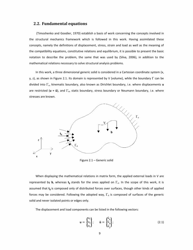
mathematical relations necessary to solve structural analysis problems
In this work, a three dimensional generic solid is considered
y, z), as shown in Figure 2.1. Its domain is represented by
divided into Γu, kinematic boundary
are restricted (u = ū), and Γσ, static boundary
stresses are known.
When displaying the mathematical relations in matrix form
represented by b, whereas tγγγγ stands for the ones applied
assumed that tγγγγ is composed only of distributed forces
forces may be considered. Following the adopted
solid and never isolated points or edges
The displacement and load components
x y
z
tγγγγ
Γ
9
Fundamental equations
(Timoshenko and Goodier, 1970) establish a basis of work concerning the concepts involved in
the structural mechanics framework which is followed in this work. Having assimilated
of displacement, stress, strain and load as well as the meaning of
the compatibility equations, constitutive relations and equilibrium, it is possible to present the
to describe the problem, the same that was used by (Silva, 2006), in addition to
necessary to solve structural analysis problems.
In this work, a three dimensional generic solid is considered in a Cartesian coordinate system (x,
Its domain is represented by V (volume), while the boundary
, kinematic boundary, also known as Dirichlet boundary, i.e. where displacements
static boundary, stress boundary or Neumann boundary
Figure 2.1 – Generic solid
mathematical relations in matrix form, the applied external loads in
stands for the ones applied on Γσ. In the scope of this work, it is
of distributed forces over surfaces, though other kinds of applied
Following the adopted way, Γσ is composed of surfaces of the generic
solid and never isolated points or edges only.
The displacement and load components can be listed in the following vectors:
u � ����ux
uy
uz
���� ; ū � ����ūxūyūz
���� ;
V
b
Γσ
Γu
(Timoshenko and Goodier, 1970) establish a basis of work concerning the concepts involved in
Having assimilated these
of displacement, stress, strain and load as well as the meaning of
present the basic
in addition to the
in a Cartesian coordinate system (x,
(volume), while the boundary Γ can be
, i.e. where displacements u
or Neumann boundary, i.e. where
, the applied external loads in V are
n the scope of this work, it is
over surfaces, though other kinds of applied
faces of the generic
(2.1)

2.2.1. Equilibrium conditions
Let σσσσ be the stresses vector (Figure
of the components of the unit outward normal vector associated with the differential operator
σ � ��������������������
σxx
σyy
σzz
σyz
σxz
σxy��������������������
; D =
�������������������� ∂
∂x0
0∂
∂y
0 0
then, the equilibrium conditions come as follows:
Figure 2
10
b � ����bx
by
bz
���� ; tγγγγ � �txγtyγtzγ
� .
Equilibrium conditions
Figure 2.2), D the equilibrium differential operator and
of the components of the unit outward normal vector associated with the differential operator
0
0
∂
∂z
0∂
∂z
∂
∂y
∂
∂z0
∂
∂x∂
∂y
∂
∂x0 !!!!
!!!!!!!!"""" ; N = ####nx 0 0
0 ny 0
0 0 nz
0 nz n
nz 0 nny nx 0
then, the equilibrium conditions come as follows:
D σσσσ + b = 0 in V,
N σσσσ = tγγγγ on Γσ .
2.2 – Three-dimensional stress element
(2.2)
and N the matrix
of the components of the unit outward normal vector associated with the differential operator D:
ny
nx
0$$$$ ; (2.3)
(2.4)
(2.5)
11
In Figure 2.2, nine components are represented whereas σσσσ lists only six. In fact the symmetry of
the stress tensor allows this simplification. The same holds true in the strains’ case.
2.2.2. Compatibility conditions
Considering D* as the compatibility differential operator and that the strains are listed in vector
εεεε, where:
εεεε � ��������������������ε%%ε&&ε''γ&'γ%'γ%&��������
������������
, (2.6)
the compatibility conditions are:
D* u = εεεε in V, (2.7)
u = ū on Γu. (2.8)
Since the assumption of geometric linearity is assumed to be valid, D and D* are adjoint
differential operators, meaning:
D*ij = (-1)n+1 Dji , (2.9)
considering n as the order of the derivative of Dji.
2.2.3. Constitutive relationship
The adopted constitutive relationship is nonlinear, which allows for the use of a more accurate
model of concrete’s behaviour. The tensor which materializes this relation is designated by K� and is a
fourth-order tensor relating two second-order tensors, σσσσ and εεεε, by the following equation:
σσσσ = K� : εεεε . (2.10)
In terms of flexibility, the nonlinear flexibility constitutive tensor is F�, yielding:
εεεε = F� : σσσσ . (2.11)
Nevertheless, the behaviour of concrete may be considered linear elastic under certain limits,
strictly speaking, while strains are smaller than those that cause crack initiation and have never
before been higher, i.e., while the material is undamaged:
12
K� = K and F� = F , (2.12)
where K and F represent, respectively, the stiffness tensor and the flexibility tensor in elastic
regime.
Although σσσσ and εεεε are second-order tensors, they are written as vectors as explained before.
Consequently, the fourth-order tensors K�, K, F� and F must be written as matrices.
Whereas K� and F� depend on the evolution of damage, K and F are constant and valid throughout
the elastic regime:
K = E(1+ν*(1−2ν* ��������1 - ν ν ν 0 0 0
ν 1 - ν ν 0 0 0
ν ν 1 - ν 0 0 0
0 0 0 0.5 - ν 0 0
0 0 0 0 0.5 - ν 0
0 0 0 0 0 0.5 - ν !!!!!!" , (2.13)
F = 1E
������� 1 -ν -ν 0 0 0
-ν 1 -ν 0 0 0
-ν -ν 1 0 0 00 0 0 2 + 2ν 0 00 0 0 0 2 + 2ν 00 0 0 0 0 2 + 2ν !
!!!!" . (2.14)
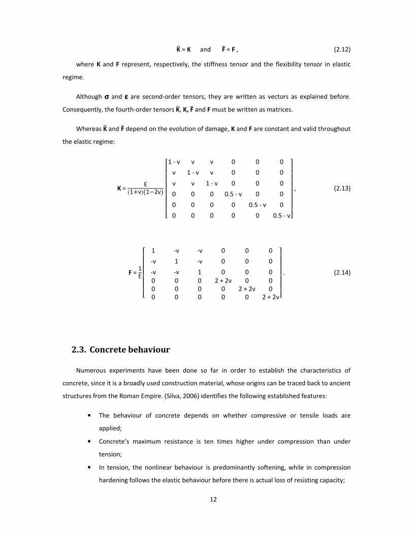
2.3. Concrete behaviour
Numerous experiments have been done so far in order to establish the characteristics of
concrete, since it is a broadly used construction material, whose origins can be traced back to ancient
structures from the Roman Empire. (Silva, 2006) identifies the following established features:
• The behaviour of concrete depends on whether compressive or tensile loads are
applied;
• Concrete’s maximum resistance is ten times higher under compression than under
tension;
• In tension, the nonlinear behaviour is predominantly softening, while in compression
hardening follows the elastic behaviour before there is actual loss of resisting capacity;
13
• In a post-peak situation, in both cases, there is permanent and irreversible loss of both
stiffness and resistance.
The deformational response of a typical concrete specimen is depicted in Figure 2.3 and
illustrates the aforesaid characteristics.
(a) Tension (b) Compression
Figure 2.3 – Experimental results for stress-strain behaviour under uniaxial loading (Mazars, 1984)
It is known that the physically nonlinear behaviour of concrete is mainly due to cracking with
origin in tensile stresses. This process starts with localized damage growth occurring at the
microscale, yet concrete is brittle at the mesoscale. This, according to (Lemaitre, 1992), means that
two scales of analysis have to be taken into account and, hence, damage is classified as quasibrittle,
instead of brittle. Modelling this type of behaviour is the aim of this work.
The quasibrittle behaviour of concrete under tension is conditioned by its heterogeneity,
namely, the existence of defects and the linking strength in the interface of the phases that comprise
the material. Moreover, a bigger structure is likely to have more defects, which might be more
compromising in some situations, for instance, in case all cross sections are critical (a beam subject to
pure bending), or not so much if the critical zone of maximum stresses is reduced to a section (mid-
span of a simply supported beam subject to self-weight, for instance). Experiments prove that
damage does not confine to zones of infinitesimal thickness of the structure, but evolves in all
directions, in what is called the fracture process zone, which size is, in fact, influenced by local
heterogeneities and by the local state of stress. On the other hand, it is independent from the
dimensions of the structure as long as it does not interfere with the boundaries of the considered
body. (Haidar et al, 2005) identify this finite size zone as the cradle of the progressive material

14
damage, which starts with rather diffuse microcracks that, as load increases, coalesce and form
macrocracks. (Haidar et al, 2005) relate this phenomenon to size effect. In fact, the ratio of the
volume of the fracture process zone to the volume of the structure varies in geometrically similar
specimens with different dimensions, which is the base of size effect on the structural strength. This
phenomenon can be reduced to a probabilistic description of damage initiation and propagation, as
(Mazars et al, 1991) have proven. Besides this, the same authors define additionally a deterministic
approach of size effect independent from initial defects, which is related to the evolution of damage
before failure in quasibrittle heterogeneous materials such as concrete.
In this work, two purely deterministic continuous damage models using one variable alone are
applied to simulate the average material degradation, which includes nucleation and growth of voids,
cavities, microcracks and other microscopic defects, occurring in the fracture process zone, according
to (Voyiadjis, 2005). Although the consequences of damage evolution, as presented by (Mazars et al,
1991), are reduction of the effective cross section, decrease of the stiffness of the material, possible
damage-induced anisotropy, irreversible strains and changes of volume as well as potential internal
friction, the models presented in this work only focus on the stiffness reduction using continuum
damage models for this is enough to include size effect and model cracking in the performed
analysis. In fact, the nonlinear physical analysis performed by (Silva, 2006) with non-conventional
finite elements was also based on continuum damage models. According to the same author, this is
particularly accurate when failure comes as the result of microcracks that lead to bigger cracks. Other
models, such as fracture models, should be used if there is knowledge of the localization of cracking
in advance.
However, given the fact that damage evolves due to cracking, there is an apparent incoherence
in choosing a continuum damage model over a fracture model. Nevertheless, (Bažant, 1984) adverts
that this is not an unrealistic procedure since strain softening accurately models the distribution of
microcracking and can even give results consistent with the tortuous forms of the path of a final
crack, not to mention the advantages related to finite element modelling. Even those who oppose
the continuum damage models, arguing that they do not represent a physical law, agree that it
provides a simplification to the constitutive relations that concurs with physical observations for
many materials (Dvorkin and Goldschmit, 2005).
Altogether, it is evident that concrete’s behaviour is far from being simple and so is its
description. In fact, under tension, damage-induced anisotropy is visible at a macroscopic level and
make it inaccurate to try to build a stress-strain diagram because these local variables cannot
reproduce the behaviour of the whole concrete specimen. Therefore, the best way to describe an
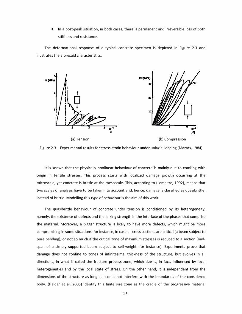
15
experiment with relevant tensile stresses is with a load-displacement curve, which is unique for each
case. A typical result in case of uniaxial tension would be that of Figure 2.4.
Figure 2.4 – Qualitative description of concrete’s behaviour under a uniaxial tension experiment (Silva, 2006)
As depicted in Figure 2.4, the behaviour of concrete under uniaxial tension starts as linear
elastic. The maximum tensile force is registered already with some diffuse microcracking and almost
no hardening. The evolution of the extensions results in crack concentration in the fracture process
zone; in this phase, softening is clear with significant loss of both stiffness and resistance. Towards
the end of the experiment, the fracture process zone gets narrower and narrower, tending to a
fracture plane. At this point, discrete crack models models are interesting alternatives to continuum
damage models, since diffuse microcracking turns into coalescent macrocracks. According to (Comi
et al, 2002), this way, the three steps of the physically nonlinear behaviour of Figure 2.4 are
modelled:
1. Diffuse micro-cracking
2. Strain-softening localization in the fracture process zone
3. Crack initiation and propagation.

16
17
3. Damage models
3.1. Initial considerations
Continuum damage mechanics has been evolving for the past 50 years. In terms of solid
mechanics, damage is defined by (Lemaitre and Desmorat, 2005) as “the creation and growth of
microvoids or microcracks which are discontinuities in a medium considered as continuous at a larger
scale”, implying permanent loss of stiffness and resistance.
Among various possible models, in order to keep the emphasis of this work in the possibility of
adding damage to the hybrid displacement formulation without making it inefficient and to avoid
unnecessarily complex formulations, a simple version of isotropic continuum damage is chosen, the
Mazars damage model, proposed by (Mazars, 1984), which is adequate to model concrete’s
quasibrittle behaviour under monotonic loading. In this model, derived from pure phenomenological
constitutive relations, the stiffness elastic tensor is multiplied by a scalar variable of damage. Besides
this, Comi and Perego’s damage model, introduced by (Comi and Perego, 2001) is also applied,
enabling comparisons between the results thus obtained and those of (Silva, 2006).
The determination of damage may yield from either a local or nonlocal point of view. A local
continuum damage model would only be accurate if there were materials which could be analysed as
continua even at an infinitesimal level. There is no such thing and, besides, concrete is not a
continuous medium even to the naked eye. So, first, attention is given to the fact that, as stated by
18
(Terada and Asai, 2005), a failure criterion should not be based on local values because of their
mesh-dependence, which is a consequence of their non-smooth distribution. The smoothing process
that solves this problem is technically related to a regularization methodology and is based on a
localization limiter which is set in such a way that altogether the real behaviour of the structures is
correctly modelled. Preference is given in this work to a nonlocal damage model rather than to a
model based on the fracture energy. In fact, (Häussler-Combe and Pröchtel, 2007) state that nonlocal
damage models are attractive due to their physical meaning, which relates the existence of
heterogeneities to the concept of characteristic length, and because they fit smoothly into the
classical continuum approach. Also, mesh-objectivity is preserved while mesh-bias of localization is
avoided with relatively simple numerical methods. On the contrary, fracture energy regularization
models do not preserve mesh-objectivity and present mesh-bias of localization, as, in fact, only the
global behaviour is regularized. (Silva, 2006) presents these models as applicable only in case of
structures of great size.
Another step, less obvious than the ones before, is to choose the nonlocal physical quantity to
be obtained by performing weighted averaging of the corresponding local quantity as well as the
weighting function, bearing in mind that only the variables that cause strain softening should be
considered as nonlocal (Bažant and Lin, 1988). Only then the model is complete. In this chapter, this
path leads to a nonlocal version of Mazars damage model and of Comi and Perego’s damage model.
The thermodynamic principles that are the cornerstone of these formulations are not presented
due to their complexity and because of the limited scope of this work. Nevertheless, different
bibliographic sources are suggested.
3.2. Nature of the phenomenon
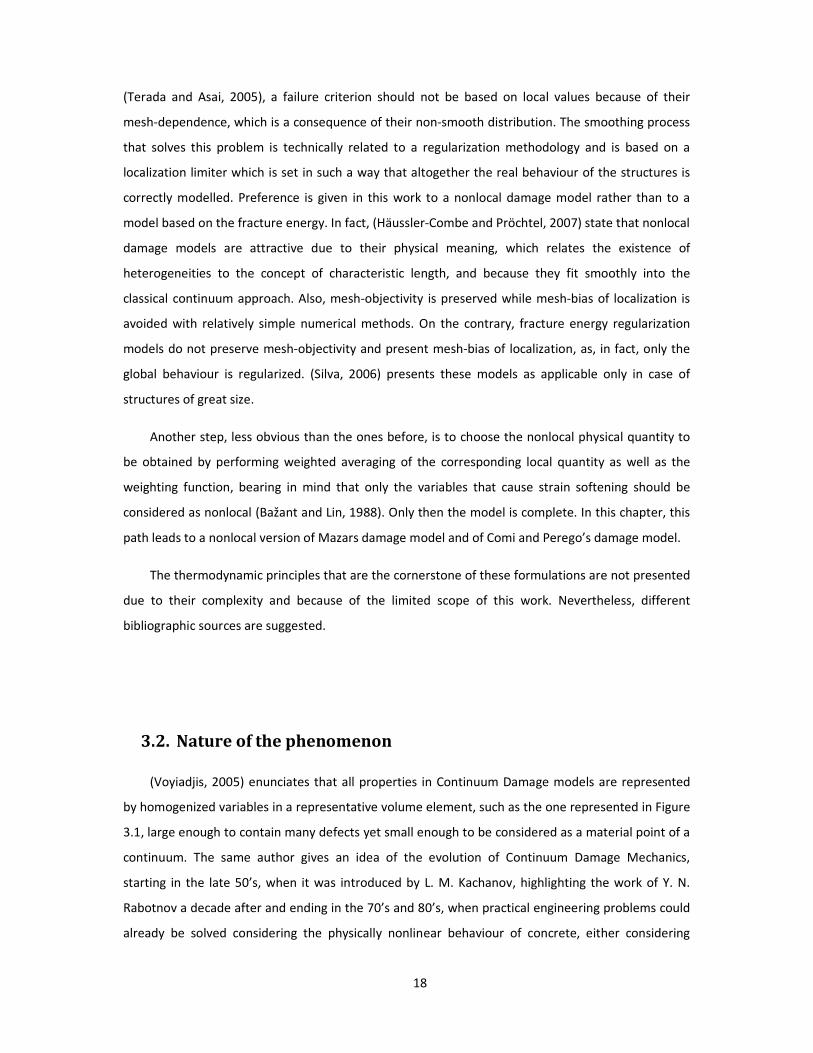
(Voyiadjis, 2005) enunciates that all properties in Continuum Damage models are represented
by homogenized variables in a representative volume element, such as the one represented in Figure
3.1, large enough to contain many defects yet small enough to be considered as a material point of a
continuum. The same author gives an idea of the evolution of Continuum Damage Mechanics,
starting in the late 50’s, when it was introduced by L. M. Kachanov, highlighting the work of Y. N.
Rabotnov a decade after and ending in the 70’s and 80’s, when practical engineering problems could
already be solved considering the physically nonlinear behaviour of concrete, either considering
19
isotropic damage, such as in the work of J. Lemaitre and J. L. Chaboche, or anisotropic damage, like in
the work of J. P. Cordebois and F. Sideroff . This way the origins of the following mathematical
formulation can be traced. Nowadays, applications of isotropic and anisotropic damage models cover
also dynamic problems, porous materials and chemical damage. Examples are cited by (Kotronis et
al, 2007).
Figure 3.1 – Representative volume element in a damaged solid (Silva, 2006)
Considering an area with a normal n�� of the representative volume element, S, an effective
resisting area, S�, is obtained by removing the surface intersections of the microcracks and cavities, as
well as correcting the micro-stress concentrations around discontinuities and the interactions
between closed defects (Voyiadjis, 2005). Hence:
S� ≤ S . (3.1)
Considering this same surface with the normal n��, the variable which represents the evolution of
damage, dn, can be computed according to the expression:
dn � S - S�S
� 1 − S�S (3.2)
The limit values of dn have, thus, a physical meaning. When there is no damaged area S = S� and
dn is equal to 0, while, as damage increases, S� approaches zero and dn approaches its maximum
value, 1. Also, it is worth noticing that irreversibility is already implicit in this formulation, whereas
the effective resisting area cannot increase and, so, dn has a monotonous behaviour.
A characteristic of an isotropic damage models is that dn is actually independent of the direction
of n��, and, therefore, can simply be represented by d, which means that it is assumed that the
microcracks and cavities due to loading are uniformly distributed in all directions (Chow and Wang,
1987).
20
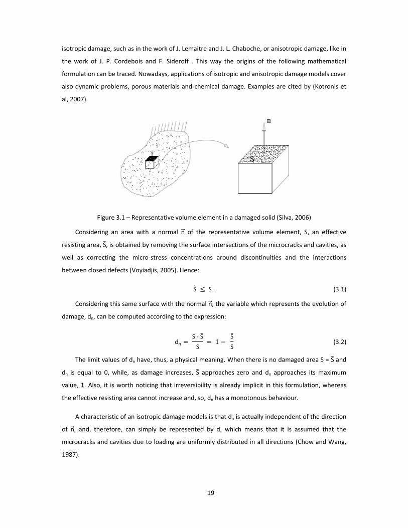
In order to derive a constitutive relation comprising damage, it is easier to start by considering a
concrete specimen under tension (uniaxial experiment) and, only after that, generalise to a three-
dimensional damage model.
First, looking at concrete as an ensemble of fibres, as in Figure 3.2, it is assumed that each fibre
has a purely elastic brittle behaviour and that they all have the same initial stiffness E, even though
their maximum resistant strains differ. While there is no damage, all fibres have the same strain, ε,
and, hence, equal stress, σ. Once the maximum resistant strain of one of the fibres is achieved, the
fibre collapses and tension is immediately redistributed. From this point on, there is a distinction
between the stress, which still considers the original area, S, and the effective stress, σ � , which is
computed on the basis of the undamaged area, S�. Also, it is considered that the principle of strain
equivalence is valid. This way, the strain constitutive equations for the damaged material are derived
from the same formalism as for a non-damaged material except that the stress is replaced by the
effective stress (Lemaitre and Desmorat, 2005). These assumptions are coherent with the applied
damage models. However, were the damage models anisotropic, the principle of strain equivalence
should be replaced by the principle of energy equivalence, which is more general (Silva, 2006). These
models entail the shape and size of the defects so that the effective resisting area can be computed,
requiring, according to (Voyiadjis, 2005), mathematical homogenization techniques and studies
based on electron microscopy, which are far from being desirable in the present state of work.
Figure 3.2 – Uniaxial damage model using the principle of strain equivalence (Silva, 2006)
Knowing that the principle of strain equivalence states that the strain behavior of a damaged
material is represented by the constitutive equations of the undamaged material provided that the
stress is simply replaced by the effective stress (Lemaitre, 1992), it is immediate that Hooke’s law
should be written in terms of effective stresses:
σ = E ε . (3.3)
L
. = ./ 0 = 0
L+ΔL’
1 = 0 . = 0 ./
. = ./ 0 = 0 ≠ 0
L+ΔL’’
1 = 0 . = 0 ./
. ≠ ./ 0 ≠ 0
21
The effective stress is defined as the stress in the undamaged state, which corresponds to the
effective resisting area, yielding:
σ � = FS� =
σ S
S� . (3.4)
It is possible to manipulate (3.2) in order to combine it with (3.3) and (3.4), so that the following
relationship is deduced:
σ = (1 – d) E ε . (3.5)
Instead of the Young’s modulus, a stiffness matrix K can be applied for a more general situation,
yielding the secant stiffness relation:
σσσσ = (1 – d) K εεεε , (3.6)
where d is a function which expresses the law of damage in terms of a variable chosen
accordingly to the considered damage model.
From (3.6), it is plain that d can also be viewed as a direct measure of the loss of secant stiffness
of the material.
A more complete approach to damage mechanics is presented in (Lemaitre and Desmorat,
2005), where the three steps of modelling different materials’ behaviour is explained according to
the thermodynamics of irreversible processes. Summarizing briefly in order to introduce the applied
damage models, these three steps are:
1. Definition of state variables, which might be observable or internal and are used to
characterize the state of the mechanism. The choice of the state variables depends on the
physical mechanisms of damage;
2. Definition of a state potential, such as the Helmholtz specific free energy (Ψ) used in
Continuum Damage Mechanics, and of the variables associated with the internal state
variables. In this step, the laws of thermoelasticity are derived;
3. Definition of a dissipation potential, f. The kinetic laws governing the evolution of the state
variables associated with the dissipative mechanisms are derived in this step.
It is worth noticing that, as it is explained by (Lemaitre and Desmorat, 2005), the definitions
applied at each step must meet the experimental results and purpose of use, yielding various
damage models. For instance, in the models applied in this work, the dissipation potential is written
in terms of two variables, generically called a and k, where a and k are either associated variables
(Comi and Perego’s model) or state variables (Mazars model), and is given by the expression:
22
f(a,k) = a – k, with k(t) = max { max τ ≤ t [a (τ)], k0] (3.7)
where t stands for time, and k is equal to a threshold value k0 until this limit is overcome by a;
from there on, it takes the maximum value reached by a.
Furthermore, when modelling a material with no viscosity under static or quasi-static loading,
time is not relevant. Based on this premise, the complete loading or unloading conditions, also
known as Kuhn-Tucker conditions, might be derived yielding:
f ≤ 0, k3 ≥ 0, f k3 = 0. (3.8)
3.3. Comi and Perego’s damage model
(Comi and Perego, 2001) propose an isotropic damage model dependent on one scalar variable
alone, d, which stands as an internal state variable. Another internal state variable, ξ, is introduced in
equation (3.9) to define the Helmholtz specific free energy (Ψ) and has a kinematic nature. The
strains (εεεε) play the role of observable state variables. The associated variables are the stress vector σσσσ
(equation (3.10)), the elastic energy release rate Y (equation (3.11)) and the thermodynamic force χ
(equation (3.12)). These variables are defined in terms of the derivatives of Ψ with respect to each
state variable:
Ψ = 12
(1 - d* ε : K : ε + Ψin(ξ) ; (3.9)
σ = ∂Ψ
∂ε= (1 - d) K : ε , (3.10)
Y = -∂Ψ
∂d = 1
2 ε : K : ε , (3.11)
χ = ∂Ψ
∂ξ = Ψ'in(ξ) . (3.12)
In equation (3.9), Ψin(ξ) expresses the inelastic energy density, so that microstructural
rearrangements due to damage evolution are taken into account.
The dissipation potential is written in terms of Y and χ, according to the following equation:
f (Y – χ* = Y – χ = 12
ε : K : ε – χ ≤ 0 (3.13)
The evolution of the internal variables is defined in terms of the derivatives of the dissipation
potential with respect to the associated variables. Hence:
23
d3 = ∂f
∂Y γ3 = γ3 , ξ3 = − ∂f
∂χ γ3 = γ3 , (3.14)
in which γ is a positive scalar. As a consequence of the above equations, the damage variable d
takes the same value of the internal variable ξ and of the positive scalar γ, defining that they are all
null before damage is initiated.
Furthermore, (Comi and Perego, 2001) propose the following expression to determine the
inelastic energy density:
Ψin(ξ) = k (1 – ξ) ∑ n!i!
ni=0 lni : c
1- ξ; (3.15)
yielding
χ = ∂Ψ
∂ξ = k lnn < c
1- ξ=, (3.16)
which requires the calibration of the parameters k, n and c to model the behaviour of the
material.
The damage initiation threshold of this model in case of uniaxial damage is ε0 = >k lnn(c) 2
E. For
strains greater than this, the behaviour of the material is nonlinear with exponential softening and, if
the parameters are chosen with that purpose, also with a hardening zone between linear elasticity
and softening. The unloading process is modelled elastically, which means there are no permanent
strains.
The original version of this model does not differentiate between the behaviour of the material
under compression or tension, which is not realistic. Therefore, an additional condition is imposed so
that damage only exists if the trace of the strains tensor is greater than zero. This quantity is
independent of the coordinate system and is called the volumetric strain. Imposing that it has to be
greater than zero is the same as restricting the evolution of damage to points of the structure where
elongation occurs. Consequently, this model is mainly adequate to structures essentially under
tensile stresses.
24
3.4. Mazars damage model
In this work, Mazars damage model is also used to add physically nonlinear effects to the
analysis of concrete structures. As introduced by (Mazars, 1984), one single scalar damage variable is
used, called d, that depends only on the tensile strains of the material. The latter are observable
state variables and the former is an internal state variable. In order to consider only the tensile
extensions, the mathematical formulation uses the Macaulay brackets, ? ( @. @* A+, which work in the
following way: ? ( @. @* A+ = ½ [ ( . ) + | ( . ) | ] and, thus, return the value of the argument if it is positive
and zero otherwise. It is also possible to return the value of the argument if it is negative and zero
otherwise, which is also introduced with pointed brackets, ? ( @. @* A-, and is implemented with the
following algorithm: ? ( @. @* A- = ½ [ ( . ) - | ( . ) | ]. Another characteristic of Mazars model is the
absence of permanent strains, even though the material’s plasticity and viscosity, as well as the
damage process itself, make them inevitable in reality (Figure 2.3 a) according to (Paula, 2001) and
(Pituba, 1998).
In a three-dimensional space the strain is a tensor field, meaning the magnitude of the strain in
a certain point of the structure depends not only on the localization of the point but also on a
direction of analysis. Therefore, according to Mazars model, an equivalent strain ε is used, which
attempts to summon the tensor field to a single observable state variable, ε � ε(ε). This value aims
to define the accumulated tensile strain in the material, as stated in (Mazars et al, 1991) and, hence,
assembles the positive principal strains in the following way:
ε = >?εIA+2+?εIIA+
2+?εIIIA+2= >∑ ?εiA+
2IIIi=I . (3.17)
First, the appearance of damage is controlled by an initial damage threshold εd0, which must be
calibrated to meet the behaviour observed in a uniaxial tension experiment (Proença, 1992). Then,
the law of damage evolution d = d(ε) must be formulated in such a way that:
1. Damage has a null value if the initial damage threshold has never been reached;
2. The model respects the fact that damage is irreversible;
3. The variable d approaches progressively the unit as the strains increase.
Since these assumptions must be applicable to more complex strain fields than just uniaxial
loading (Pituba, 1998), the dissipation potential of Mazars damage model (third step mentioned in
section 3.2.) is a function of the equivalent strain:
f(ε,d) = ε – χ (d) ≤ 0, where χ (0) = εd0 and χ (d(t)) = max { max τ ≤ t [ ε (τ)], εd0]. (3.18)

25
The kinetic laws governing the evolution of damage yield:
d3 = 0 if f < 0 or f = 0 and f3 < 0; (3.19)
d3 = F(ε* ?ε3AB if f = 0 and f3 = 0. (3.20)
F(ε) is a continuous and positive function of the equivalent strain such that damage increases
whenever the equivalent strain increases. This function is different whether its purpose is to model a
uniaxial compression or tension state, which results in the definition of two independent scalar
variables, dc and dt respectively. These variables describe the evolution of damage due to
compression and tension, according to the following mathematical expressions:
d3t = Ft(ε* ?ε3 AB , (3.21)
d3c = Fc(ε* ?ε3 AB , (3.22)
where,
Ft(ε) = εd0 (1- At)
ε2 + At Bt
exp[BtC ε - εd0D] , (3.23)
Fc(ε) = εd0 (1- Ac)
ε2 + Ac Bc
exp[BcC ε � -εd0D] . (3.24)
The integration of expressions (3.21) and (3.22) is provided in the literature already cited and
yields:
dt (ε) = 1 – εd0 (1- At)
ε – At
exp[BtC ε-εd0D] , (3.25)
dc (ε) = 1 – εd0 (1- Ac)
ε – Ac
exp[BcC ε-εd0D] . (3.26)
These expressions are applicable only if the equivalent strain is greater than the initial damage
threshold; otherwise damage is equal to zero. Furthermore, parameters At and Bt (related to tension)
and AC and BC (related to compression) are, just like εd0, material parameters that have to be
calibrated based on experiments on cylinders, the first-named under uniaxial tension with controlled
deformations and the last-named under uniaxial compression with controlled displacements (Mazars
et al, 1991).
Initially, (Mazars, 1984) proposed the following:
0.7 ≤ At ≤ 1 104 ≤ Bt ≤ 105 10-5 ≤ εd0 ≤ 10-4
1 ≤ Ac ≤ 1.5 103 ≤ Bt ≤ 2 × 10³ (3.27)
26
These parameters assure that hardening only occurs in compression.
One of the advantages of this damage model is that these relatively simple assumptions and
expressions can be generalised to more complex states of stress, retaining the concept of only one
damage variable d, which is obtained by linear combination of (3.25) and (3.26):
d = αt dt + αc dc , (3.28)
constraining parameters αt and αc to observe αt + αc = 1. This way, bending tests on beams may
also be performed to calibrate the parameters, according to (Kotronis et al, 2007). The same authors
propose that αt and αc should be replaced by αtβ and αc
β, so that the behaviour of concrete under
shear may be reproduced more accurately. The value 1.06 is indicated for β. Nevertheless, these
considerations were not taken into account in this work and the original version of Mazars model is
used. The values for both parameters αt and αc are determined according to (Perego, 1990):
αt = ∑ ?εTiA+
IIIi=I∑ ?εTiA+
IIIi=I + ∑ ?εCiA+
IIIi=I
(3.29)
and
αc = ∑ ?εCiA+
IIIi=I∑ ?εTiA+
IIIi=I + ∑ ?εCiA+
IIIi=I
, (3.30)
being
εTi = 1+ν
E ?σ iA + –
ν
E ∑ ?σ jA+
IIIj=I I (3.31)
and
εCi = 1+ν
E ?σ iA – –
ν
E ∑ ?σ jA-
IIIj=I I. (3.32)
In the previous expressions, I is the identity tensor and σ i/σ j are the principal effective stresses.
As expected, under uniaxial tension αt = 1 and for uniaxial compression αc = 1.
The application of this damage model to the constitutive relation is achieved in the secant form
by:
σσσσ = (1 – d) K εεεε (3.33)
having, hence, d affecting all the entries of the elemental elastic stiffness matrix in the same
way.
27
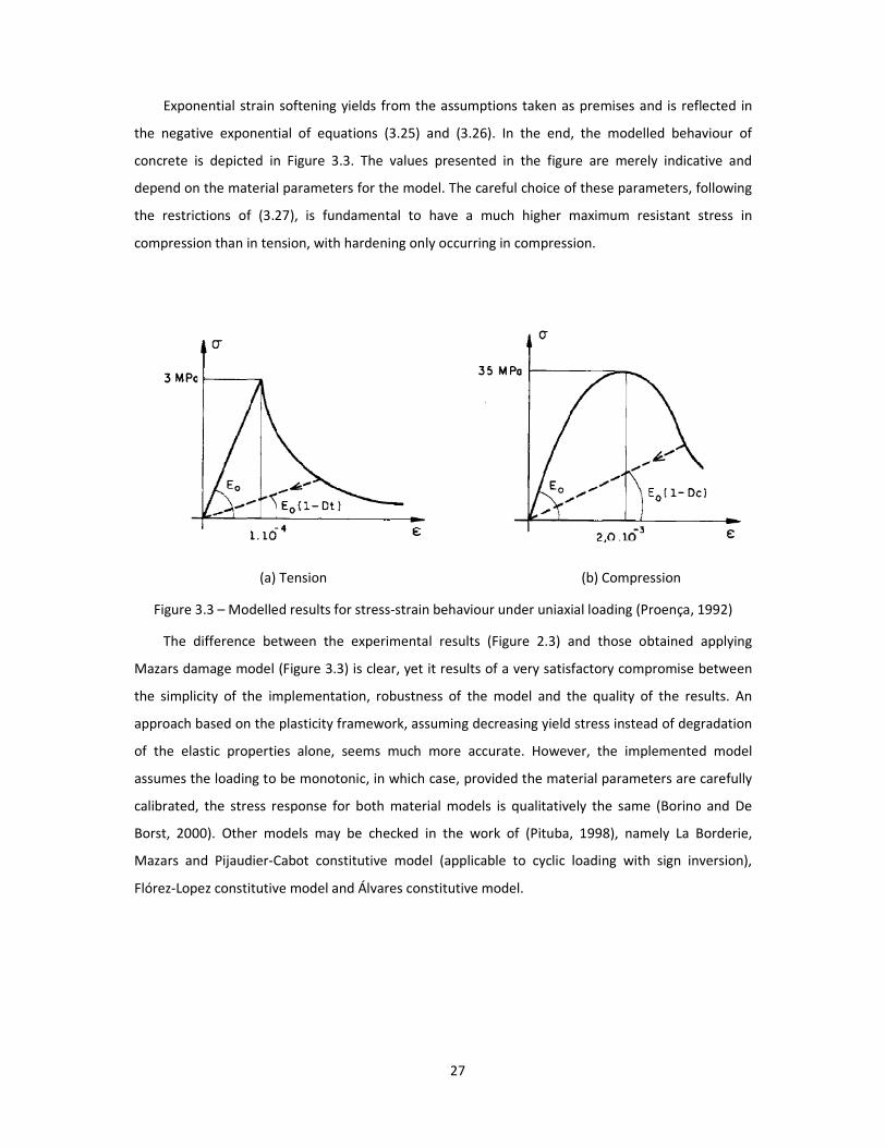
Exponential strain softening yields from the assumptions taken as premises and is reflected in
the negative exponential of equations (3.25) and (3.26). In the end, the modelled behaviour of
concrete is depicted in Figure 3.3. The values presented in the figure are merely indicative and
depend on the material parameters for the model. The careful choice of these parameters, following
the restrictions of (3.27), is fundamental to have a much higher maximum resistant stress in
compression than in tension, with hardening only occurring in compression.
(a) Tension (b) Compression
Figure 3.3 – Modelled results for stress-strain behaviour under uniaxial loading (Proença, 1992)
The difference between the experimental results (Figure 2.3) and those obtained applying
Mazars damage model (Figure 3.3) is clear, yet it results of a very satisfactory compromise between
the simplicity of the implementation, robustness of the model and the quality of the results. An
approach based on the plasticity framework, assuming decreasing yield stress instead of degradation
of the elastic properties alone, seems much more accurate. However, the implemented model
assumes the loading to be monotonic, in which case, provided the material parameters are carefully
calibrated, the stress response for both material models is qualitatively the same (Borino and De
Borst, 2000). Other models may be checked in the work of (Pituba, 1998), namely La Borderie,
Mazars and Pijaudier-Cabot constitutive model (applicable to cyclic loading with sign inversion),
Flórez-Lopez constitutive model and Álvares constitutive model.
28
3.5. Comparison of both damage models in uniaxial tensile tests
It is clear now that Comi and Perego’s model and Mazars model have very distinct premises and
formulations. To model the same structures with both, it is necessary to calibrate the material
parameters for each model on the basis of the results obtained, preferentially in a load-displacement
curve. Nevertheless, already in an early stage of this work, stress-strain diagrams in case of uniaxial
tension were computed in order to have a more accurate sensitivity of the influence of the material
parameters on each damage model.
The derivation of an expression for Mazars damage evolution is presented in the previous
section and, thus, equation (3.25) is applied in this section.
Taking equation (3.16), assuming ξ to be equal to d, and bearing in mind that damage evolves
when equation (3.13) corresponds to an equality, Comi and Perego’s evolution of damage law yields:
d = 1 – c
exp E >YkFn G . (3.34)
Considering a concrete specimen under uniaxial tension with controlled deformations and
disregarding, for the sake of simplicity, Poisson’s effect, ε � ε and Y = 1
2 E ε2, which makes the
comparison between models much easier and that is enough at this level. A full comparison between
models is possible when modelling structures and comparing load-displacement diagrams instead of
stress-strain diagrams, due to the reasons exposed in the previous chapter.
Equation (3.24) makes it clear that, according to Mazars model, damage can be decomposed as
the unit minus a constant over the strain minus a negative exponential function of the strain, while,
according to Comi and Perego’s model, damage is the result of the unit minus a negative exponential
function of the strain to the power two over n. Therefore, the models render the same stress-strain
diagram when, in Comi and Perego’s model, n = 2 and, in Mazars model, εd0 =>k lnn(c) 2
E , At = 1.0 and
Bt = >E2 kFn
. Hence, for instance, with E = 30000 GPa, choosing Comi and Perego’s parameters:
k = 1.5 × 10⁻⁴ MPa, c = 2.72 and n =2, Mazars parameters for a perfect match must be At = 1.0,
Bt = 10 000 and εd0 = 10-4. Figure 3.4 and Figure 3.5 attest this perfect match between the two
models, first by giving damage as a function of the strains and afterwards by displaying the yielding
stress-strain diagrams.
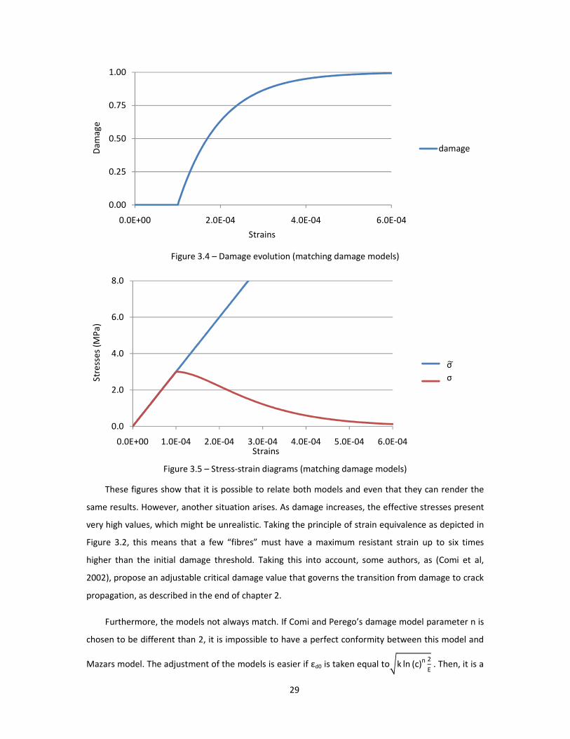
29
Figure 3.4 – Damage evolution (matching damage models)
Figure 3.5 – Stress-strain diagrams (matching damage models)
These figures show that it is possible to relate both models and even that they can render the
same results. However, another situation arises. As damage increases, the effective stresses present
very high values, which might be unrealistic. Taking the principle of strain equivalence as depicted in
Figure 3.2, this means that a few “fibres” must have a maximum resistant strain up to six times
higher than the initial damage threshold. Taking this into account, some authors, as (Comi et al,
2002), propose an adjustable critical damage value that governs the transition from damage to crack
propagation, as described in the end of chapter 2.
Furthermore, the models not always match. If Comi and Perego’s damage model parameter n is
chosen to be different than 2, it is impossible to have a perfect conformity between this model and
Mazars model. The adjustment of the models is easier if εd0 is taken equal to>k ln (c)n 2
E . Then, it is a
0.00
0.25
0.50
0.75
1.00
0.0E+00 2.0E-04 4.0E-04 6.0E-04
damage
0.0
2.0
4.0
6.0
8.0
0.0E+00 1.0E-04 2.0E-04 3.0E-04 4.0E-04 5.0E-04 6.0E-04
~σ
σ=(1-d)~σ
σ �
σ Stre
sses
(M
Pa)
Strains
Strains
Dam
age
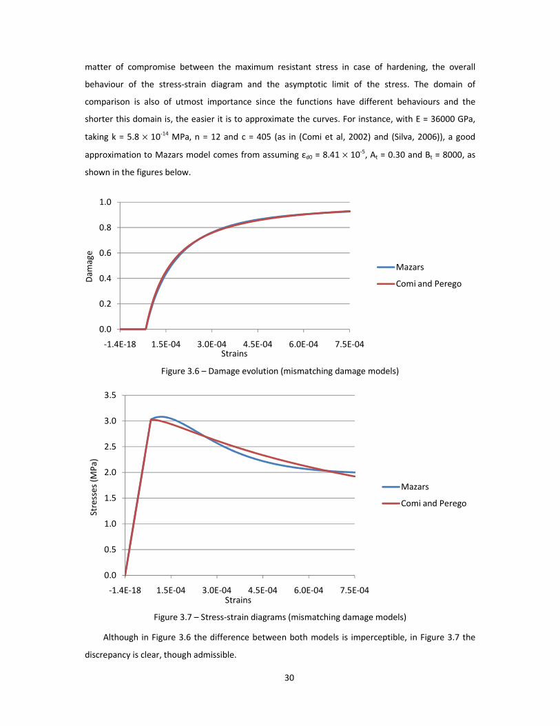
30
matter of compromise between the maximum resistant stress in case of hardening, the overall
behaviour of the stress-strain diagram and the asymptotic limit of the stress. The domain of
comparison is also of utmost importance since the functions have different behaviours and the
shorter this domain is, the easier it is to approximate the curves. For instance, with E = 36000 GPa,
taking k = 5.8 × 10⁻¹⁴ MPa, n = 12 and c = 405 (as in (Comi et al, 2002) and (Silva, 2006)), a good
approximation to Mazars model comes from assuming εd0 = 8.41 × 10⁻⁵, At = 0.30 and Bt = 8000, as
shown in the figures below.
Figure 3.6 – Damage evolution (mismatching damage models)
Figure 3.7 – Stress-strain diagrams (mismatching damage models)
Although in Figure 3.6 the difference between both models is imperceptible, in Figure 3.7 the
discrepancy is clear, though admissible.
0.0
0.2
0.4
0.6
0.8
1.0
-1.4E-18 1.5E-04 3.0E-04 4.5E-04 6.0E-04 7.5E-04
Mazars
Comi and Perego
0.0
0.5
1.0
1.5
2.0
2.5
3.0
3.5
-1.4E-18 1.5E-04 3.0E-04 4.5E-04 6.0E-04 7.5E-04
Mazars
Comi and Perego
Dam
age
Strains
Stre
sses
(M
Pa)
Strains
31
3.6. Strain localization and regularization methods
Mazars damage model takes damage directly as a function of the strain field, while in Comi and
Perego’s model damage is computed considering the elastic energy release rate, which, nevertheless,
is a function of the strain field. Since the strain field varies from one point of the structure to
another, damage itself is a space-dependent variable. However, the result thus obtained without
further refinement is not reliable once it leads to an unrealistic concentration of high magnitude
strains. Besides, damage concentrates in an element which is smaller if the mesh is refined, up to a
point when failure occurs in a layer of infinitesimal thickness and without dissipation of energy,
according to (Bažant, 1984) and (Mazars et al, 1991). However, this strain localization is not the only
problem as there is also a phenomenon of loss of ellipticity presented by (Lemaitre et al, 2002),
which is related to the ill-posedness of the boundary value problems, leading to an infinite number of
linearly independent solutions that might not depend continuously on the data. On the whole, a local
change of the type of the boundary value problem during a loading process in a physically nonlinear
analysis from elliptic to hyperbolic may happen. The same authors give the example of the
appearance of discontinuity surfaces in softening materials.
According to (Skrzypek et al, 2008), in case viscosity is taken into account, the ellipticity of the
problem is retained, which means that well-posedness is preserved, since length-scale measures are
implicitly introduced by viscosity, thus, reducing strain and damage localization. The same authors
give examples of work in this area as well as in nonlocal combined viscosity and in gradient-enhanced
theory of anisotropic thermo-plastic-damage. However, as (Pijaudier-Cabot and De Borst, 2002)
indicate, viscosity should control both the fracture energy and the evolution of the material strength
with the loading rate and this is not always in accordance with experimental data. On the other hand,
if viscosity is not accounted for, the solution is to apply regularization methods, which play the
transition from a very localized deformation behaviour to a diffuse one, in order to solve the above
mentioned problems that the classical local continuum framework fails to describe. These problems
are clearly presented by (Silva, 2006):
1. Numerical problem: the solution is mesh-dependent, i.e., the answer is not objective
2. Physical problem: there is a limit situation of infinite deformation associated with no energy
dissipation. Besides, heterogeneity of the microstructure and microcrack interaction are
being neglected;
3. Mathematical problem: the boundary value problem becomes ill-posed.
32
Regularization methods can be derived either from the concept of fracture energy or by
applying nonlocal continuum damage. The techniques based on a fracture energy and on the
influence volumes (three-dimensional elements) of the integration points are not used, despite their
easy implementation and physical intuitiveness. According to (Silva, 2006), one of the drawbacks
associated with fracture energy regularization methods appears because the numerical problem is
not solved and the only way to minimize this is to apply homothetic mesh refinements. Besides,
these approaches can model a more ductile behaviour than the real one, which obviously carries
safety problems. Therefore a nonlocal integral averaging model is the elected regularization method
because, according to (Silva, 2006), it is simpler to implement and more robust. However, (De Borst
and Guitiérrez, 1999) find fully nonlocal damage approaches employing spatially averaged quantities
to be computationally unwieldy. This discrepancy is due to the fact that (Silva, 2006) used non-
conventional finite elements and this makes the difference, since a p-refinement can be done in a
much easier way in these elements than in conventional finite elements. In fact, the alternative h-
refinements, which are associated with generating a new mesh, would imply a determination at each
step of the required points to perform the regularization process, which is necessarily based on a
quadrature rule. As one of the advantages of non-conventional finite elements, namely a hybrid
displacement model, is the use of macro-elements, the basis of the nonlocal model might be a sub-
mesh of the global mesh that does not change along the refinement process. The sub-mesh is built
with integration points related to the used quadrature rule. This work in particular is developed using
Lobatto points, which include points on the boundary of the considered interval, unlike Gauss
quadrature (Beyer, 1987).
Nonlocal damage models must verify the stress dissipation of the local model and both models
must return the same results in elastic regime and during unloading. (Bažant and Pijaudier-Cabot,
1988) expose that nonlocal behaviour assumes there is a spatial weighting of the variables that cause
strain softening, and only these, as if blurring is applied to them. In order to do so, a parameter to
control the magnitude of this spatial weighting is defined. In these studies, a characteristic length l is
used, regulating the weight of the analysed neighbourhood centered at each evaluation point
(Mazars et al, 1991). According to these authors, the characteristic length should be taken
proportional to the smallest width of the region in the medium into which damage can coalesce,
which experimentally means around three times the size of the largest heterogeneity in the material.
This mathematical stratagem is, ultimately, a way of considering the interaction between microcracks
(Silva, 2006). Because in this model the constitutive relation in a certain point depends on the
behaviour of the structure around the evaluation point, it is called “strongly nonlocal”, whereas
33
others, such as the gradient models, are called “weakly nonlocal” and involve differential equations
to introduce the effects of spatial regularization.
The mathematical implementation of the nonlocal integral averaging model is achieved by using
a nonlocal variable aH, which has an effect either on the constitutive relation or on the dissipation
potential. The analytical expression of this variable is:
aH(x) = I W(x,s* a(s* dVV
(3.35)
where x is the location where the quantity is evaluated, s is the general coordinate vector, V is
the volume of the entire body and W(x,s) is a weighting function. (Bažant and Lin, 1988) treat this
function as a material property and advice the choice of a smooth function for better convergence. In
this work, as well as in (Comi et al, 2002) and (Silva, 2006), the normalized Gaussian weight function
serves this purpose:
W(x,s) = 1
W0(x) exp #– Jx-sJ2
2 l2 $ (3.36)
with
W0 (x) = I exp #– Jx-sJ2
2 l2 $ dV
V . (3.37)
The normalization condition (3.37) is necessary to assure that, when the local quantity is
homogeneous, the equivalent nonlocal variable is homogeneous too.
The previous integrals are approximately evaluated as finite sums over all the integration points
in the defined finite element mesh. This way, it is not a problem the fact that the normal distribution
functions extend beyond the volume, because only the values in the integration points are
considered (Bažant and Lin, 1988).
The nonlocal physical quantity indicated for Comi and Perego’s model is the elastic energy
release rate, Y (Comi et al, 2002), whereas for Mazars damage model it is the equivalent strain, ε
(Mazars et al, 1991). In this way, the goal of considering damage as nonlocal is achieved.
It is worth to underline that, as (Terada and Asai, 2005) point out, the weighted averaging plays
only a role of regularization of the non-smooth distribution of the strains in order to assess the
magnitude of damage. It is not applied directly to the governing equation, though it appears
implicitly in the damage variable which affects the constitutive equation.

34
35
4. Finite element formulation
4.1. Initial considerations
Finite element methods represent nowadays a resourceful tool in the hands of engineers, as
they allow research to develop faster and in a greater number of fields as well as projects to be
designed in a much more competitive way than in older days. The applications of finite element
methods are numerous and their main purpose is to model reality as accurately as possible.
However, exact solutions are restricted to very specific cases, namely academic examples, and can no
longer be found as structural and load complexity increases. The approximation that current finite
element methods reach has one main advantage, which is the fact that it is strongly related to the
displacement method and, hence, has a very solid theoretical background, as it has been object of
study of structural analysis for many years. Nevertheless, it is also true that this method provides
unsafe solutions according to the kinematic theorem of plastic analysis. On the other hand, a solution
which fulfils the conditions of the static theorem corresponds to a safe solution. The finite element
formulation developed in this dissertation is not under any of the above theorems; however, at least,
it is not straightforward that the given solution is not safe for the structure, as in conventional
formulations, even though this particular non-conventional finite element models are targeted to
produce kinematically admissible solutions and hence they are likely to overvalue the resisting
capacity of the structure.
In this chapter, after a brief background concerning the non-conventional finite element
formulations developed by the Structural Analysis Research Group of Instituto Superior Técnico, the
36
derivation of this formulation is exposed following the line of thought developed by (Freitas et al,
1999). Bearing in mind that the first step, which is the formulation of the fundamental relations
governing the problem being modelled, is done in the previous chapters, the starting point that is
specific of this formulation is the approximation criteria. After that, the finite element equations are
established, which finally leads to the derivation of the governing system of equations and to the
establishment of the model’s theoretical framework.
4.2. Hybrid displacement model as a non-conventional finite
element formulation
The formulations developed by the Structural Analysis Research Group of Instituto Superior
Técnico and designated as “non-conventional” in this dissertation are not the only alternatives to the
conventional finite element method. However, they derive from four hypotheses presented by
(Freitas, 1989) which make them distinctive from the others:
1. The alternative formulations are directly deduced from the relevant principles of mechanics
presented in section 2.2.1;
2. The generalised variables of the discrete model are defined in an energetically consistent
way by imposing the equivalence between the work of dual quantities in the discrete and
continuous models;
3. Nodes are only necessary to define the geometry of the structure, letting go the concept of
nodal interpolation and allowing the use of nodeless, hierarchical approximation functions;
4. The theorems of Mathematical Programming allow the recovery of the corresponding
variational theorems associated to the non-conventional formulations and the
establishment of the conditions for existence, uniqueness and stability of solutions.
Consequently, (Freitas et al, 1999) present three sets of hybrid finite element formulations, each
one comprising two possible distinct models: displacement models or stress models. The
formulations were named hybrid-mixed, hybrid and hybrid-Trefftz. A hybrid model comes from a
mixed-hybrid model. Whereas the latter is derived without imposing any conditions in the domain,
1 In this work, neither residual stresses nor strains are considered. However, this does not compromise the introduction of these quantities in the model, which is possible and can be found in (Freitas, 1998) and in (Freitas and Pereira, 1991).

37
the former obliges approximation functions to verify locally either compatibility or equilibrium
conditions in the domain. In the first case the model is called hybrid displacement model, otherwise
it is a hybrid stress model. Developing a hybrid displacement model, equilibrium is enforced in the
domain in the weak form and the connection between adjacent elements is achieved by means of
imposing compatibility, which implies that the inter-element boundary is considered kinematic. On
the whole, independent approximations of both the displacement field in the domain of each finite
element and the field of applied stresses along the kinematic boundary lead to this finite element
formulation. Besides, the constitutive equation is written in terms of stiffness, which makes it easier
to introduce damage adopting usual procedures and algorithms.
Several advantages are associated with the above mentioned “non-conventional” finite element
formulations. Among the ones pointed out by (Silva, 2006), the following have particular relevance
and are applicable to hybrid displacement models:
1. This formulation shows great flexibility when it comes to choosing the approximation
functions. In fact, any complete set of functions may be used to model the displacement
field in the domain of each finite element and the field of applied stresses along the
kinematic boundary. In the present work, orthonormal Legendre polynomials are used.
2. It is possible to use macro-elements for it is preferable to use a p-refinement instead of an
h-refinement. Therefore, complex mesh generation techniques are not a requisite to solve
structural problems.
3. If the approximation functions include particular solutions of the displacement fields in the
domain, the numerical convergence is faster and the analysis of structures with arbitrary
geometry is easier. Also, in the case of concentrated moving loads, the introduction of
particular solutions avoids the necessity of generating new meshes during the analysis.
4. With this finite element model, it is possible to choose different degrees of approximation
for the various approximated fields, because they are independent from each other.
However, some drawbacks of these formulations have also been identified by (Silva, 2006):
1. They are conceptually more complex, namely in terms of discretization and approximation.
2. The physical sense of nodal forces or nodal displacements is replaced by weights of the
approximation function since the concept of nodal interpolation is no longer valid.
3. The governing systems have a large number of degrees of freedom and are highly sparse in
elastic regime. On the one hand, it is possible to use techniques which take advantage of
both sparsity and symmetry of the systems to save computational memory. On the other
hand, this kind of resolution is less intuitive and suggests some reluctance from users.
38
4. Spurious modes may appear and it is adequate to minimize them by choosing correctly the
degrees of the various approximations.
5. The matrix of the governing system is not positive-definite. Despite that, it is possible to
solve the equations set if there are no dependencies.
4.3. Mathematical description of the hybrid displacement model
Hybrid displacement models are characterized by independent approximations of both the
displacement field in the domain of each finite element, u, and the field of applied stresses along the
kinematic boundary, which includes the boundaries between elements, tγγγγ. These approximations can
be written in the following way:
u = UV q in V, (4.1)
tγγγγ = T p on Γu. (4.2)
The approximation functions for the displacements in the domain are listed in the matrix Uv and
the matrix T stores the approximation functions for the stresses along the kinematic boundary of
each element. Unlike the conventional formulation, these approximation functions do not enforce
compatibility between elements and with the imposed displacements. Therefore, equation (4.1) is
not enough and a second approximation is necessary. The hybrid formulation allows them to be
independent from each other and to have different values in each direction of the coordinate
system. Vectors q and p list the weights associated to each approximation, displacements in the
domain and stresses on the kinematic boundary, respectively. In conventional formulations, the
approximation functions are enforced so that the vectors represent nodal quantities. In this non-
conventional formulation, one can only call them generalised displacements in the domain in the
case of q and generalised stresses on the kinematic boundary in the case of p.
The generalised forces in the domain, QV, and the generalised displacement along the kinematic
boundary, v, may be defined by imposing that the dual quantities in the continuous and discrete
models perform the same work (Freitas et al, 1999). Therefore:
QV = ∫ UVT b dV, (4.3)
v = ∫ TT ū dΓu . (4.4)
39
The equilibrium in the domain is enforced on average, resulting in the weak formulation of the
balance laws:
∫ UVT (D σσσσ - b) dV = 0. (4.5)
Similarly, when the same reasoning is applied to the compatibility along the kinematic
boundary, the following expression is deduced:
∫ TT (u - ū) dΓu = 0. (4.6)
The following expression results from the integration by parts of (4.5) taking (4.3) into account:
– ∫ (D* UV)T σσσσ dV + ∫ (N* UV)T
σσσσ dΓu + ∫ (N* UV) T σσσσ dΓσ = – QV . (4.7)
An equilibrium equation comes from working the previous expression, considering the assumed
constitutive relation, the derived compatibility equation in the domain and the equilibrium relation
on the boundary, as well as the approximations established in (4.1) and (4.2). It is then possible to
write:
� q – B p = QV + QΓΓΓΓ in V, (4.8)
with:
� = ∫ (D* UV)T K� (D* UV) dV, (4.9)
B = ∫ (UV)T T dΓu , (4.10)
QΓΓΓΓ = ∫ (UV) T tγγγγ dΓσ . (4.11)
The compatibility equation along the kinematic boundary is also necessary to solve the problem
and emerges from including the approximations defined in (4.1) in (4.6):
– BT q = – v on Γu. (4.12)
Combining (4.8) and (4.12), the governing system to solve a problem using a hybrid
displacement model is symmetric and given by:
K � - B- BT
0L Mq
pN = OQV + QΓ
- v P (4.13)
It is worth noticing that the operator BT alone is responsible for binding elements and is
therefore called the compatibility operator. Furthermore, the deduced expressions assume that the
loads are distributed on surfaces. The drawback is that particular load cases such as prescribed
displacements along edges or punctual forces can only be applied after revising the equilibrium
equation (4.7).

40
41
5. Computational application
5.1. Initial considerations
This chapter links the previous one, where the theoretical background of the hybrid
displacement models is introduced, with the following one, where results of the modelling process
are presented. In order to do so, further details of the computational part of the work are given,
namely on the implementation and the analytical expressions which allow for the computation of the
operators.
The implementations of the models were made both in MATLAB®2 and FORTRAN. The author
worked with MATLAB® and the results thus obtained for simple examples were compared with the
ones provided by the program written in FORTRAN, namely for physically nonlinear analysis of two-
dimensional structures and elastic analysis of three-dimensional structures. The more complex
structures were modelled using only the FORTRAN implementation, due to its better performance.
The visualizations of the tensor fields and of the deformed configuration of the structures were
possible with MayaVi3.
This chapter includes the implementation steps and the structure of the finite element program,
with special attention being drawn to the aspects which are particular of this formulation, namely
the derivation of the used mathematical expressions.
2 MATLAB version 7.6.0.324 (R2008a) – http://www.mathworks.com
3 MayaVi Data Visualizer version 1.5 – http://mayavi.sourceforge.net/
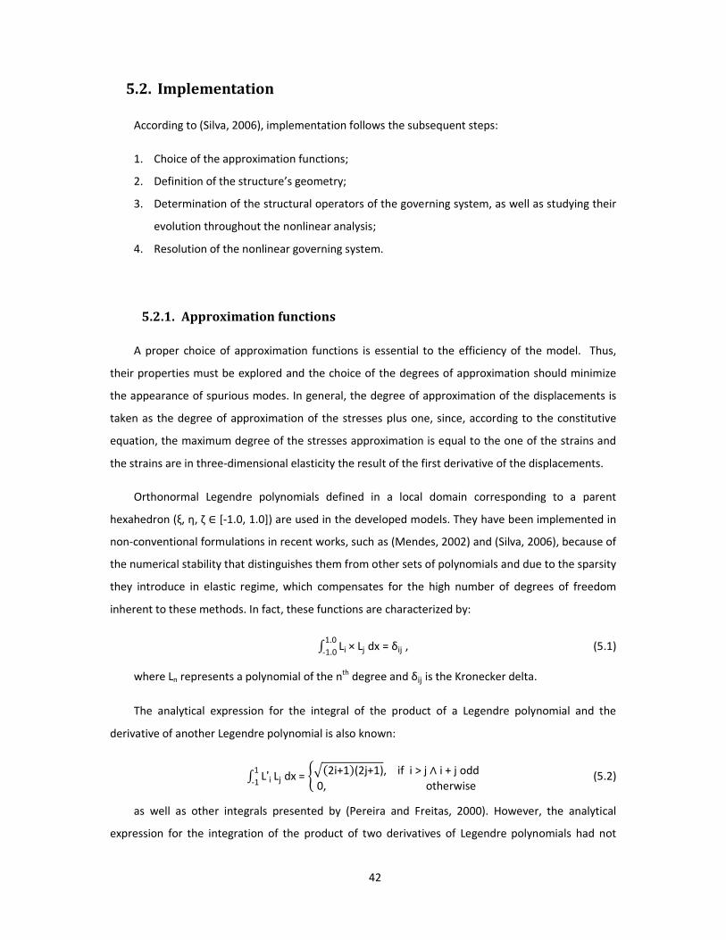
42
5.2. Implementation
According to (Silva, 2006), implementation follows the subsequent steps:
1. Choice of the approximation functions;
2. Definition of the structure’s geometry;
3. Determination of the structural operators of the governing system, as well as studying their
evolution throughout the nonlinear analysis;
4. Resolution of the nonlinear governing system.
5.2.1. Approximation functions
A proper choice of approximation functions is essential to the efficiency of the model. Thus,
their properties must be explored and the choice of the degrees of approximation should minimize
the appearance of spurious modes. In general, the degree of approximation of the displacements is
taken as the degree of approximation of the stresses plus one, since, according to the constitutive
equation, the maximum degree of the stresses approximation is equal to the one of the strains and
the strains are in three-dimensional elasticity the result of the first derivative of the displacements.
Orthonormal Legendre polynomials defined in a local domain corresponding to a parent
hexahedron (ξ, η, ζ ∈ [-1.0, 1.0]) are used in the developed models. They have been implemented in
non-conventional formulations in recent works, such as (Mendes, 2002) and (Silva, 2006), because of
the numerical stability that distinguishes them from other sets of polynomials and due to the sparsity
they introduce in elastic regime, which compensates for the high number of degrees of freedom
inherent to these methods. In fact, these functions are characterized by:
I Li1.0
-1.0× Lj dx = δij , (5.1)
where Ln represents a polynomial of the nth degree and δij is the Kronecker delta.
The analytical expression for the integral of the product of a Legendre polynomial and the
derivative of another Legendre polynomial is also known:
I L'i1
-1Lj dx = OR(2i+1*(2j+1), if i > j ∧ i + j odd
0, otherwise@ (5.2)
as well as other integrals presented by (Pereira and Freitas, 2000). However, the analytical
expression for the integration of the product of two derivatives of Legendre polynomials had not
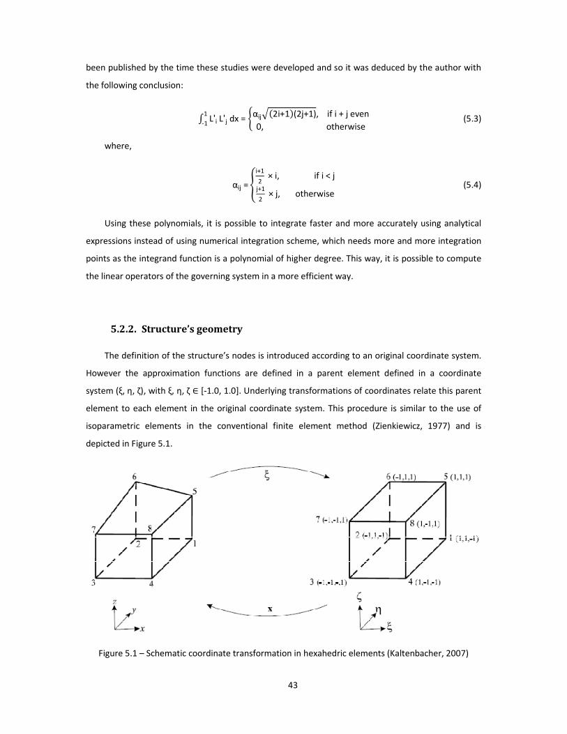
43
been published by the time these studies were developed and so it was deduced by the author with
the following conclusion:
I L'i1
-1L'j dx = OαijR(2i+1*(2j+1), if i + j even
0, otherwise@ (5.3)
where,
αij = �i+1
2 × i, if i < j
j+1
2 × j, otherwise
@ (5.4)
Using these polynomials, it is possible to integrate faster and more accurately using analytical
expressions instead of using numerical integration scheme, which needs more and more integration
points as the integrand function is a polynomial of higher degree. This way, it is possible to compute
the linear operators of the governing system in a more efficient way.
5.2.2. Structure’s geometry
The definition of the structure’s nodes is introduced according to an original coordinate system.
However the approximation functions are defined in a parent element defined in a coordinate
system (ξ, η, ζ), with ξ, η, ζ ∈ [-1.0, 1.0]. Underlying transformations of coordinates relate this parent
element to each element in the original coordinate system. This procedure is similar to the use of
isoparametric elements in the conventional finite element method (Zienkiewicz, 1977) and is
depicted in Figure 5.1.
Figure 5.1 – Schematic coordinate transformation in hexahedric elements (Kaltenbacher, 2007)
44
5.2.3. Structural operators
The difference between an elastic and a physically nonlinear analysis is that the operator �
must be updated in successive load steps because its entries depend on the evolution of damage in
the structure. As analysis develops, this operator, which starts as a sparse matrix modelling the linear
behaviour, is potentially full in nonlinear regime. Anyway, � is a symmetric matrix and advantage is
taken from this by computing only the necessary entries to define the whole operator. On the
contrary, the operators v, QV, QΓΓΓΓ and B are analytically computed in the beginning of the modelling
process using the expressions derived in the previous section and there is no need to recompute
them as damage evolves.
The expressions derived in chapter 4 for the structural operators consign that the used integrals
are defined in the original coordinate system (structure in a three dimensional space: x, y, z).
However, the approximation functions, which appear in UV and T, are defined in a local coordinate
system (parent element defined by three coordinates: ξ, η, ζ). Therefore, a coordinate transformation
is necessary, such as shown in Figure 5.1, involving the Jacobian of the coordinate transformation
from the parent element to the global coordinate system, |J|.
Taking Ln as the orthonormal Legendre polynomial of the nth degree defined in [-1.0, 1.0], a
possible organization of the matrix UV is to build three blocks,UV x, UV y and UV z, considering that, in
general, the degrees of the approximations can be distinct in each direction. Each block is, in fact,
one row with (nv x + 1)3, (nv y + 1)3 or (nv z + 1)3 columns, respectively for each direction. Assuming that
nv x = nv y = nv z = nv, the column [i (nv + 1)2 + j (nv + 1) + k + 1] of each block allocates the polynomial
Li(x) Lj(y) Lk(z), yielding:
UV = #⋯ Li(x* Lj(y* Lk(z* ⋯ ⋯ 0 ⋯ ⋯ 0 ⋯⋯ 0 ⋯ ⋯ Li(x* Lj(y* Lk(z* ⋯ ⋯ 0 ⋯⋯ 0 ⋯ ⋯ 0 ⋯ ⋯ Li(x* Lj(y* Lk(z* ⋯$ (5.5)
where i, j and k are integers varying from 0 to nv.
On the other hand, there is a different T matrix for each possible orientation of the kinematic
boundaries. Since the program is targeted to structures where the finite element meshes are made
of rectangular prisms, the definition of the T matrices is standard. For instance, in case of a face
which is perpendicular to the y-axis, the Legendre polynomials may only vary in x and z, yielding, for
instance:
45
T = # ⋯ Lm(x* Ln(z* ⋯ ⋯ 0 ⋯ ⋯ 0 ⋯⋯ 0 ⋯ ⋯ Lm(x* Ln(z* ⋯ ⋯ 0 ⋯⋯ 0 ⋯ ⋯ 0 ⋯ ⋯ Lm(x* Ln(z* ⋯ $ (5.6)
where m and n are integers varying from 0 to ng and Lm(x) Ln(z) is the entry of the column
[m (ng +1) + n + 1] of each block, summing (ng +1)2 entries. Also in this case, it is possible to define
different degrees of approximation by distinguishing ng x, ng y and ng z, yet the model was designed
accepting only one value as the degree of approximation for the stresses along the kinematic
boundary.
Bearing in mind that:
B = ∫ (UV)T T dΓu (5.7)
and still considering the illustrative example of a face perpendicular to the y-axis, for instance,
contained in the plane y = b, of a finite element that, for a more precise description, is defined in a
three-dimensional space confined to x ∈ [0, a], y ∈ [0, b] and z ∈ [0,c],
B = I I (a
0
c
0UV (x,y,z) |y=b )T
T (x,z) dx dz. (5.8)
However, Legendre polynomials are not defined in these coordinates, but in (ξ, η, ζ ∈ [-1.0, 1.0]).
Therefore, a coordinate transformation is performed, resulting:
B = I I (1
-1
1
-1UV (ξ,η,ζ) | η=1 )T
T (ξ, ζ) a c
4 dξ dζ. (5.9)
Both matrices Uv and T are block diagonal matrices, hence, the product defined in (5.9) is also a
block diagonal matrix, each block with (nv + 1)3 lines and (ng + 1)2 columns. The entry in the line
[i (nv + 1)2 + j (nv + 1) + k + 1] and in the column [m (ng +1) + n +1] of each block is then given by:
Bi,j,k,m,n = I I (1
-1
1
-1 Li(ξ* Lj(1* Lk(ζ* Lm(ξ) Ln(ζ) )
a c
4 dξ dζ. (5.10)
Taking into consideration the properties of orthonormal Legendre polynomials and realizing that
the transformation of coordinates implies a coefficient equal to the area of the element’s face over
the area of parent element’s face, the simplification of the previous expression yields:
Bi,j,k,m,n =
Face Area
4 Lj( 1* δim δkn . (5.11)
The three blocks thus determinable (one for each direction) are necessary only in case the
displacements of the face are known in all three directions and in inter-element boundaries. In fact,
the only blocks that are computed are those associated with kinematic boundaries, i.e., a couple
face-direction with known displacement. One last point about the compatibility operator is that, in
46
the developed program, the local coordinate systems are defined in such a way that the same
direction in two adjoining boundaries is positive in the perspective of one element and negative the
other way round. Compatibility is then assured just multiplying the result of expression (5.11) by (-1)
when the element face corresponds to either ξ = -1, η = -1 or ζ = -1.
The right-hand-side of the governing system is also computed regardless of damage. First, from
QV = ∫ UVT b dV , (5.12)
it is evident that the vector QV may be analyzed as the integral of three blocks, UV xT bx, UV y
T by
and UV zT bz. These three blocks comprise one larger block that expresses the generalized body-forces
on each finite element. The derivation of a simpler formula for the first block of any finite element
leads to the following expression for the entry [i (nv + 1)2 + j (nv + 1) + k + 1], which considers the
body-forces to be constant,
QVi,j,k
= Finite element volume
2 √2 bx, if i = j = k = 0 and 0 otherwise, (5.13)
meaning that, in this case, only the first entry of each block may be different than zero.
The computation of the other blocks only requires bx to be replaced by either by or bz.
The generalized body forces on the static boundary are computed according to
QΓΓΓΓ = ∫ (UV) T tγγγγ dΓσ . (5.14)
This vector is composed of three blocks per element as well. Also in this case, each block refers
to one of the possible directions of the load. For instance, supposing that the finite element defined
in the example given for the compatibility operator has tyγ constant and different than zero on the
static boundary perpendicular to the x-axis with x = 0, the entry [i (nv + 1)2 + j (nv + 1) + k + 1] of the
second block is:
QΓΓΓΓi,j,k =
Face Area
2 Li (-1) t
yγ if j = k = 0 and 0 otherwise. (5.15)
The indexes of the previous formula depend on which boundary is being considered, while the
block depends on the direction of the load.
Finally, the generalized displacements on the kinematic boundary, defined as
v = ∫ TT ū dΓu , (5.16)
47
may also be decomposed in three blocks, one per each direction of displacement. The way the
entries are computed depends on the boundary and, for example, considering a face perpendicular
to the z-axis with a prescribed displacement parallel to the x-axis, the [i (ng +1) + j + 1] entry of the
first block is given by
vi,j =
Face Area
2 ū
x if i = j = 0 and 0 otherwise. (5.17)
Once again, the assumption that displacements must be uniform leads to the fact that only the
first entry of each block may be different from zero.
Furthermore, it seems appropriate to present the general expressions of the elastic stiffness
matrix. As a matter of fact, after damage evolution is initiated the integrals have to be computed
numerically. However, it is legitimate to compute the exact stiffness matrix first and only run the
routine that computes � after the damage threshold is reached and solely in the elements that
suffer damage. The derivations behind them reveal that each elemental matrix must be computed as
the assembly of nine sub-blocks and, therefore, all these expressions are presented only in appendix
A, to avoid being too exhaustive in this chapter.
In post-processing, the generalized displacements in V, q, are divided into blocks. Each block has
3 (nv + 1)3 entries and represents the displacements of a finite element. It may be subdivided into 3
sub-blocks, each with (nv + 1)3 entries, allowing the computation of the displacement along the x-
axis, the y-axis and the z-axis, respectively: qx, qy and qz. From basic elasticity, stresses are computed
according to:
�����
σxx
σyy
σzz
σyz
σxz
σxy�����
= E(1+ν*(1-2ν)
��������1-ν ν ν 0 0 0
ν 1-ν ν 0 0 0
ν ν 1-ν 0 0 0
0 0 0 0.5 - ν 0 0
0 0 0 0 0.5 - ν 0
0 0 0 0 0 0.5 - ν !!!!!!"
�����εxx
εyy
εzz
γyzγxzγxy��
���
. (5.18)
Once damage begins the right-hand-side of equation (5.18) returns the value of the effective
stresses.
Noting that
εεεε = D* u = D* UV q (5.19)
48
and considering that α(i,j,k) marks the entry of line [i (nv + 1)2 + j (nv + 1) + k + 1] of each sub-
block:
εxx = 2
a ∑ ∑ ∑ L'i(ξ* Lj(η)
nvk=1
nvj=1
nvi=1 Lk(ζ) qx α(i,j,k) (5.20)
εyy = 2
b ∑ ∑ ∑ Li(ξ* L'j(η)
nvk=1
nvj=1
nvi=1 Lk(ζ) qy α(i,j,k) (5.21)
εzz = 2
c ∑ ∑ ∑ Li(ξ* Lj(η)
nvk=1
nvj=1
nvi=1 L'k(ζ) qz α(i,j,k) (5.22)
γyz = 2
c ∑ ∑ ∑ Li(ξ* Lj(η)
nvk=1
nvj=1
nvi=1 L'k(ζ) qy α(i,j,k) +
2
b ∑ ∑ ∑ Li(ξ* L'j(η)
nvk=1
nvj=1
nvi=1 Lk(ζ) qz α(i,j,k) (5.23)
γxz = 2
c ∑ ∑ ∑ Li(ξ* Lj(η)
nvk=1
nvj=1
nvi=1 L'k(ζ) qx α(i,j,k) +
2
a ∑ ∑ ∑ L'i(ξ* Lj(η)
nvk=1
nvj=1
nvi=1 Lk(ζ) qz α(i,j,k) (5.24)
γxy = 2
b ∑ ∑ ∑ Li(ξ* L'j(η)
nvk=1
nvj=1
nvi=1 Lk(ζ) qx α(i,j,k) +
2
a ∑ ∑ ∑ L'i(ξ* Lj(η)
nvk=1
nvj=1
nvi=1 Lk(ζ) qy α(i,j,k) (5.25)
This way strains, stresses in elastic regime and effective stresses are known at each Lobatto
point. The layout of the effective stress field only requires a change of coordinates from the local
system to the global one, which is trivial.
5.2.4. Governing system
Since the performed analysis is physically nonlinear, an adequate process of solving the
nonlinear governing system is to implement an incremental and iterative process. Damage is, hence,
considered incrementally as the result of the load applied in successive load steps, being each step
solved by an iterative process due to the nonlinear relation between loads and strains. A secant
method is applied in the present work, even though is provides a slower convergence than Newton’s
method, since it is easier to implement. In fact, Newton’s method is based on the determination of
the derivative of the function at each step (the tangent), whereas the secant method uses a similar
but less refined concept which is the secant, thus avoiding the unwieldy process of derivative
computation. A one-dimensional example of this technique is depicted in Figure 5.2. After each
iteration, the process reaches a greater value of deformation, which means that the value of damage
has to be recomputed considering a regularization method, as discussed in chapter 3. The result is a
new inclination of the secant and, consequently, a higher value of deformation, which means that
the following iteration started. The solution converges and the iterations end when a predefined stop
criterion is met.
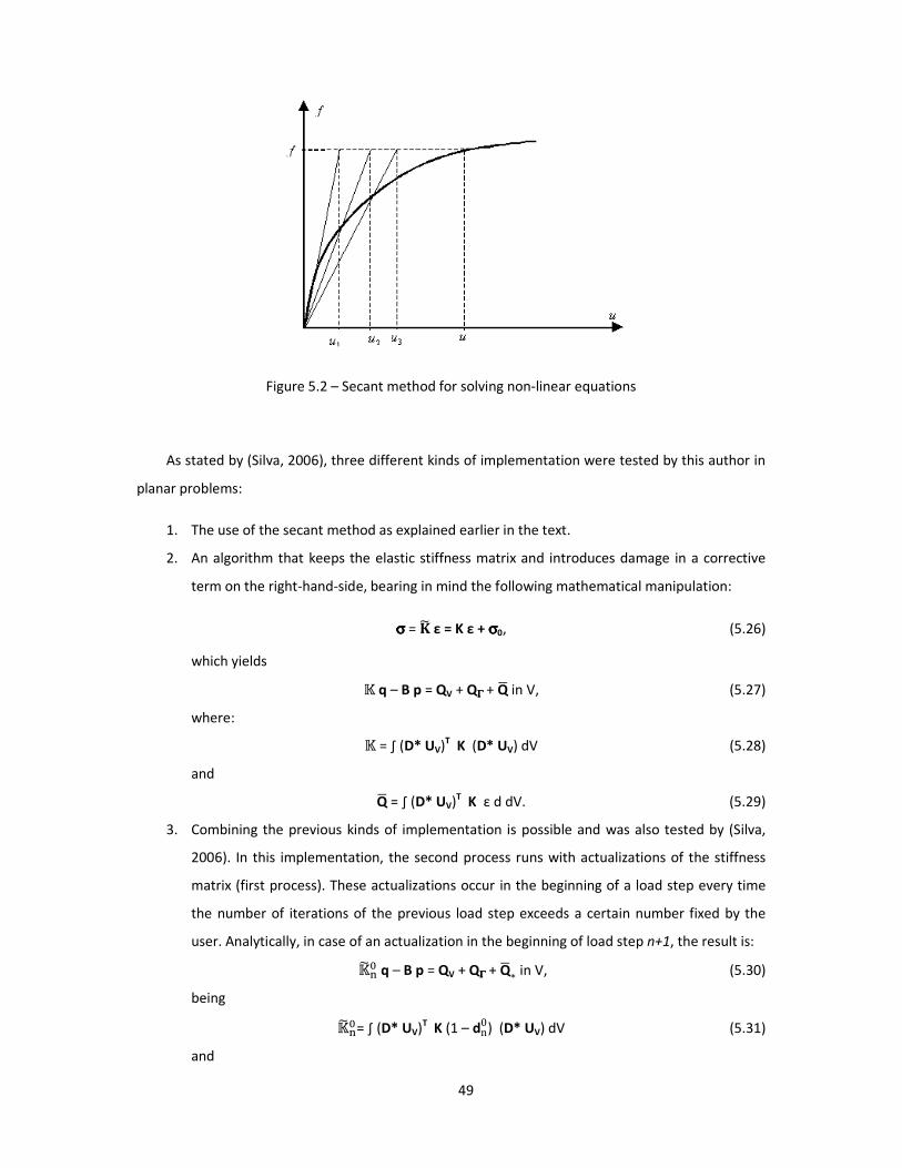
49
Figure 5.2 – Secant method for solving non-linear equations
As stated by (Silva, 2006), three different kinds of implementation were tested by this author in
planar problems:
1. The use of the secant method as explained earlier in the text.
2. An algorithm that keeps the elastic stiffness matrix and introduces damage in a corrective
term on the right-hand-side, bearing in mind the following mathematical manipulation:
σσσσ = V� ε = K ε + σσσσ0, (5.26)
which yields
q – B p = QV + QΓΓΓΓ + Q� in V, (5.27)
where:
= ∫ (D* UV)T K (D* UV) dV (5.28)
and
Q� = ∫ (D* UV)T K ε d dV. (5.29)
3. Combining the previous kinds of implementation is possible and was also tested by (Silva,
2006). In this implementation, the second process runs with actualizations of the stiffness
matrix (first process). These actualizations occur in the beginning of a load step every time
the number of iterations of the previous load step exceeds a certain number fixed by the
user. Analytically, in case of an actualization in the beginning of load step n+1, the result is:
��� q – B p = QV + QΓΓΓΓ + Q�∗ in V, (5.30)
being
���= ∫ (D* UV)T K (1 – dn0) (D* UV) dV (5.31)
and
50
Q�∗ = ∫ (D* UV)T K ε (d – dn0) dV. (5.32)
The first and second kinds of implementation were tested in the framework of this dissertation
in three-dimensional structures, but the former led to more consistent results.
5.3. Structure of the program
Two input files are called by the developed program. The first one concerns the geometry of the
structure, support conditions and the characteristics of the material (Young’s modulus, Poisson’s
ratio and either Mazars’ or Comi and Perego’s material parameters), as well as the degrees of
approximation for the displacement field in the domain of each finite element and of the field of
applied stresses along the kinematic boundary, nv and ng respectively. The second input file defines
the kinds of loading which the structure is subject to, comprising applied external loads on the static
boundary, body-forces and prescribed displacements on the kinematic boundary.
Various subroutines are called during the program in order to:
1. Compute some auxiliary values, such as the dimensions of the different structural operators,
which are functions of nv, ng and the total number of degrees of freedom.
2. Associate the number of Lobatto points per direction per element to their weights, as well
as to the values of orthonormal Legendre polynomials and their derivatives at each point.
3. Determine the three values that are sufficient to characterize the stiffness tensor in elastic
regime. Considering expression (2.13), this means advantage is taken from the fact that the
first three values of the main diagonal are equal and the same holds true for the non-
diagonal values around them and for the other three entries of the main diagonal.
4. Compute the compatibility operator (B) and the right-hand-side of the governing system
(QV, QΓΓΓΓ and v). These operators, as stated before, are independent of the existence and
evolution of damage and, hence, are computed beforehand.
5. Solve the governing system, applying an iterative process considering a monotonic
incremental evolution of the load, which follows the subsequent algorithm at each load
step:
51
a. Reset the value of the variable “Error” to ten times the predefined tolerance, the
value of the variable i (standing for iteration) to 1 and the entries of the right-hand-
side of the governing system to a fraction of the total computed in 4, multiplying QV,
QΓΓΓΓ and v by j nF , where j is the number of the load step and n the total number of
load steps.
b. While “Error” > tolerance
i. Refresh the value of i; soli-1
j stands for the solution vector and stores the
value of the solution vector computed in the previous iteration or, if it is the
first iteration of the load step, in the last iteration of the previous step;
ii. strains are computed using vector soli-1
j and, in case of Mazars damage
model, the principal strains have to be computed;
iii. a nonlocal integral averaging model with the Gaussian weight function is
applied to regularize the strains field and its values are determined at each
Lobatto point;
iv. damage is computed;
v. the nonlinear generalised elemental stiffness operator is determined
applying a Lobatto point quadrature rule.
vi. the governing system is entirely defined and the vector WR i jX, standing for
the residual right-hand-side, is computed, as well as the vector Wsol i jX both
in iteration i of load step j:
WR i jX = ORi 1j
Ri 2j
P = j nF OQV + QΓ
- v P – K � - B
- BT
0L i
j Msoli-1
j N (5.33)
YΔ sol Z = [K � - B
- BT
0L i
j\ -1 ORi 1j
Ri 2j
P (5.34)
Wsol i jX = Msoli-1
j N + YΔ sol Z (5.35)
vii. compute “Error” = ]R i j]
C , being C a normalization factor.
c. Once convergence is considered satisfactory, approximations to both the stress and
strain fields are computable for load step j and a new load increment occurs,
restarting at a., until j reaches n.
52
6. Alongside with the convergence at each load step, a post-processing subroutine creates a
.vtk file that allows for the visualization of the stress field, the damage distribution and the
deformed configuration of the structure.
53
6. Numerical tests
6.1. Initial considerations
Besides the theoretical background of the hybrid displacement formulation which has been
presented and discussed in the previous chapters, as well as the details of its implementation, this
work requires numerical tests to assess its robustness and competitiveness. Therefore, the ultimate
step of this work is to analyse the results of applying the first implementation scheme presented in
previous chapters to validate the models. Both Comi and Perego’s damage model and Mazars
damage model are tested.
First, a simple example of application of the model to an L-shaped structure is analysed, from
which a parallel with two-dimensional structures studied in an early stage of this work may be made.
The organization of the structural operators and the relevance and consequences of a p-refinement
are illustrated with this case study. Second, the behaviour of a cube under a distributed load is also
modelled, comparing attentively the results from the two damage models. In the third example, the
importance of the characteristic length is assessed in a stretched cube. Furthermore, a beam is
subject to an external distributed load first and then to body-forces to evaluate the similitude of the
results. Finally, the results of the hybrid displacement model applied to (Hassanzadeh, 1991) test are
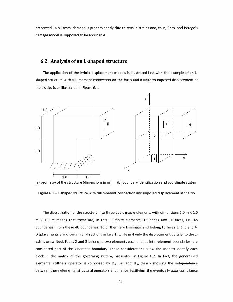
presented. In all tests, damage is predominantly due to tensile strains and, thus, Comi and Perego’s
damage model is supposed to be applicable.
6.2. Analysis of an L-shaped structure
The application of the hybrid displacement
shaped structure with full moment connection on the basis and a uniform imposed displacement at
the L’s tip, ū, as illustrated in Figure 6.1.
(a) geometry of the structure (dimensions in m)
Figure 6.1 – L-shaped structure with full moment connection and imposed displacement
The discretization of the structu
m × 1.0 m means that there are, in total, 3 finite elements, 16 nodes and 16 faces, i.e., 48
boundaries. From these 48 boundaries,
Displacements are known in all directions in face 1, while in 4 only the displacement parallel to the z
axis is prescribed. Faces 2 and 3 belong to two elements each
considered part of the kinematic boundary
block in the matrix of the governing system, presented in
elemental stiffness operator is composed by
between these elemental structural operators and, hence, justifying the eventually poor compliance
1.0
1.0
1.0
1.0 1.0
54
In all tests, damage is predominantly due to tensile strains and, thus, Comi and Perego’s
damage model is supposed to be applicable.
shaped structure
hybrid displacement models is illustrated first with the example of an L
shaped structure with full moment connection on the basis and a uniform imposed displacement at
Figure 6.1.
structure (dimensions in m) (b) boundary identification and coordinate system
shaped structure with full moment connection and imposed displacement
The discretization of the structure into three cubic macro-elements with dimensions 1.0 m
there are, in total, 3 finite elements, 16 nodes and 16 faces, i.e., 48
From these 48 boundaries, 10 of them are kinematic and belong to faces 1, 2, 3 and 4.
Displacements are known in all directions in face 1, while in 4 only the displacement parallel to the z
axis is prescribed. Faces 2 and 3 belong to two elements each and, as inter-element boundaries
considered part of the kinematic boundary. These considerations allow the user to identify each
block in the matrix of the governing system, presented in Figure 6.2. In fact, the generalised
is composed by _, ` and a, clearly showing the independence
structural operators and, hence, justifying the eventually poor compliance
ū
x
z
1
2
3
In all tests, damage is predominantly due to tensile strains and, thus, Comi and Perego’s
xample of an L-
shaped structure with full moment connection on the basis and a uniform imposed displacement at
identification and coordinate system
shaped structure with full moment connection and imposed displacement at the tip
elements with dimensions 1.0 m × 1.0
there are, in total, 3 finite elements, 16 nodes and 16 faces, i.e., 48
10 of them are kinematic and belong to faces 1, 2, 3 and 4.
Displacements are known in all directions in face 1, while in 4 only the displacement parallel to the z-
element boundaries, are
siderations allow the user to identify each
he generalised
clearly showing the independence
structural operators and, hence, justifying the eventually poor compliance
y
4
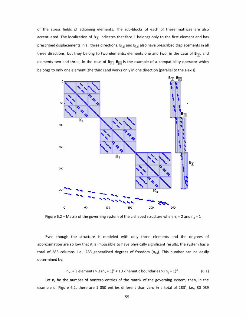
of the stress fields of adjoining elements. The sub
accentuated. The localization of B _prescribed displacements in all three directions.
three directions, but they belong to two element
elements two and three, in the case of
belongs to only one element (the third) and works only in one direction (parallel to the z
Figure 6.2 – Matrix of the governing system
Even though the structure
approximation are so low that it is impossible to have physically significant results, the system has a
total of 283 columns, i.e., 283 generalised degrees of freedom
determined by:
nsis = 3 elements ×
Let nz be the number of nonzero entries of the matrix of the governing system, then, in
example of Figure 6.2, there are 1 050 entries different than zero
_
55
of the stress fields of adjoining elements. The sub-blocks of each of these matrices are
_ indicates that face 1 belongs only to the first element
prescribed displacements in all three directions. B ` and B a also have prescribed displacements in all
they belong to two elements: elements one and two, in the case of
elements two and three, in the case of B a . B b is the example of a compatibility operator which
element (the third) and works only in one direction (parallel to the z
Matrix of the governing system of the L-shaped structure when nv = 2 and n
Even though the structure is modeled with only three elements and the degrees of
approximation are so low that it is impossible to have physically significant results, the system has a
283 generalised degrees of freedom (nsis). This number can be easily
× 3 (nv + 1)3 + 10 kinematic boundaries × (ng + 1)2 .
be the number of nonzero entries of the matrix of the governing system, then, in
, there are 1 050 entries different than zero in a total of 283
`
a
B _ B `
B
blocks of each of these matrices are also
belongs only to the first element and has
also have prescribed displacements in all
and two, in the case of B ` , and
is the example of a compatibility operator which
element (the third) and works only in one direction (parallel to the z-axis).
= 2 and ng = 1
only three elements and the degrees of
approximation are so low that it is impossible to have physically significant results, the system has a
. This number can be easily
(6.1)
be the number of nonzero entries of the matrix of the governing system, then, in the
a total of 2832, i.e., 80 089
a
B 4
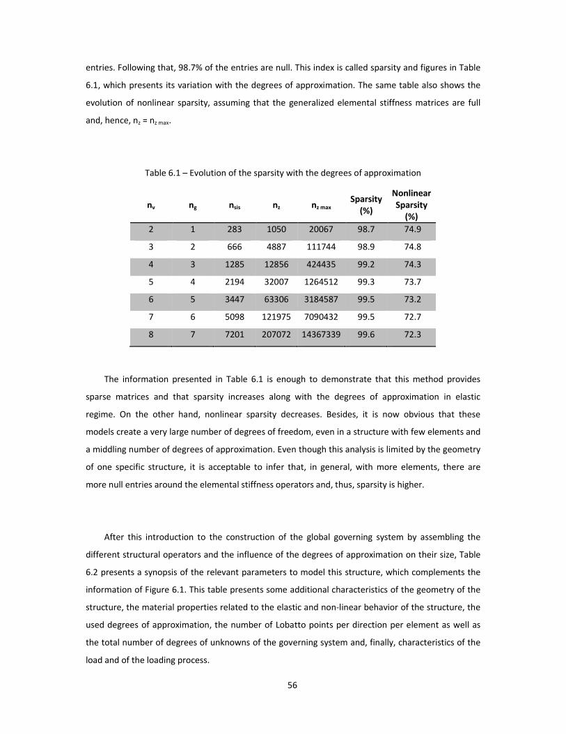
56
entries. Following that, 98.7% of the entries are null. This index is called sparsity and figures in Table
6.1, which presents its variation with the degrees of approximation. The same table also shows the
evolution of nonlinear sparsity, assuming that the generalized elemental stiffness matrices are full
and, hence, nz = nz max.
Table 6.1 – Evolution of the sparsity with the degrees of approximation
nv ng nsis nz nz max
Sparsity
(%)
Nonlinear
Sparsity
(%)
2 1 283 1050 20067 98.7 74.9
3 2 666 4887 111744 98.9 74.8
4 3 1285 12856 424435 99.2 74.3
5 4 2194 32007 1264512 99.3 73.7
6 5 3447 63306 3184587 99.5 73.2
7 6 5098 121975 7090432 99.5 72.7
8 7 7201 207072 14367339 99.6 72.3
The information presented in Table 6.1 is enough to demonstrate that this method provides
sparse matrices and that sparsity increases along with the degrees of approximation in elastic
regime. On the other hand, nonlinear sparsity decreases. Besides, it is now obvious that these
models create a very large number of degrees of freedom, even in a structure with few elements and
a middling number of degrees of approximation. Even though this analysis is limited by the geometry
of one specific structure, it is acceptable to infer that, in general, with more elements, there are
more null entries around the elemental stiffness operators and, thus, sparsity is higher.
After this introduction to the construction of the global governing system by assembling the
different structural operators and the influence of the degrees of approximation on their size, Table
6.2 presents a synopsis of the relevant parameters to model this structure, which complements the
information of Figure 6.1. This table presents some additional characteristics of the geometry of the
structure, the material properties related to the elastic and non-linear behavior of the structure, the
used degrees of approximation, the number of Lobatto points per direction per element as well as
the total number of degrees of unknowns of the governing system and, finally, characteristics of the
load and of the loading process.
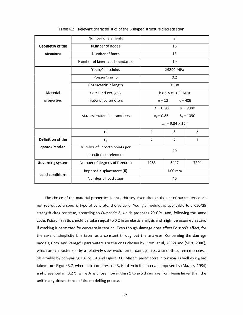
57
Table 6.2 – Relevant characteristics of the L-shaped structure discretization
Geometry of the
structure
Number of elements 3
Number of nodes 16
Number of faces 16
Number of kinematic boundaries 10
Material
properties
Young’s modulus 29200 MPa
Poisson’s ratio 0.2
Characteristic length 0.1 m
Comi and Perego’s
material parameters
k = 5.8 × 10⁻¹⁴ MPa
n = 12 c = 405
Mazars’ material parameters
At = 0.30 Bt = 8000
Ac = 0.85 Bc = 1050
εd0 = 9.34 × 10⁻⁵
Definition of the
approximation
nv 4 6 8
ng 3 5 7
Number of Lobatto points per
direction per element 20
Governing system Number of degrees of freedom 1285 3447 7201
Load conditions Imposed displacement (ū) 1.00 mm
Number of load steps 40
The choice of the material properties is not arbitrary. Even though the set of parameters does
not reproduce a specific type of concrete, the value of Young’s modulus is applicable to a C20/25
strength class concrete, according to Eurocode 2, which proposes 29 GPa, and, following the same
code, Poisson’s ratio should be taken equal to 0.2 in an elastic analysis and might be assumed as zero
if cracking is permitted for concrete in tension. Even though damage does affect Poisson’s effect, for
the sake of simplicity it is taken as a constant throughout the analyses. Concerning the damage
models, Comi and Perego’s parameters are the ones chosen by (Comi et al, 2002) and (Silva, 2006),
which are characterized by a relatively slow evolution of damage, i.e., a smooth softening process,
observable by comparing Figure 3.4 and Figure 3.6. Mazars parameters in tension as well as εd0 are
taken from Figure 3.7, whereas in compression Bc is taken in the interval proposed by (Mazars, 1984)
and presented in (3.27), while Ac is chosen lower than 1 to avoid damage from being larger than the
unit in any circumstance of the modelling process.
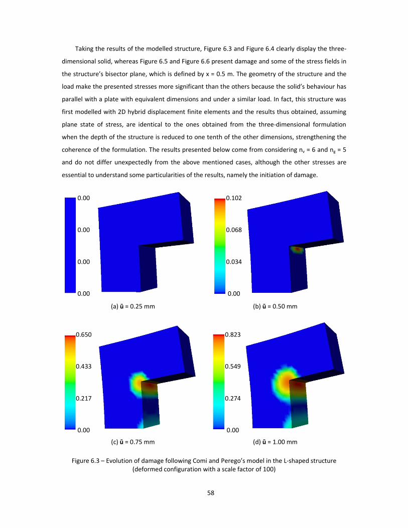
58
Taking the results of the modelled structure, Figure 6.3 and Figure 6.4 clearly display the three-
dimensional solid, whereas Figure 6.5 and Figure 6.6 present damage and some of the stress fields in
the structure’s bisector plane, which is defined by x = 0.5 m. The geometry of the structure and the
load make the presented stresses more significant than the others because the solid’s behaviour has
parallel with a plate with equivalent dimensions and under a similar load. In fact, this structure was
first modelled with 2D hybrid displacement finite elements and the results thus obtained, assuming
plane state of stress, are identical to the ones obtained from the three-dimensional formulation
when the depth of the structure is reduced to one tenth of the other dimensions, strengthening the
coherence of the formulation. The results presented below come from considering nv = 6 and ng = 5
and do not differ unexpectedly from the above mentioned cases, although the other stresses are
essential to understand some particularities of the results, namely the initiation of damage.
(a) ū = 0.25 mm (b) ū = 0.50 mm
(c) ū = 0.75 mm (d) ū = 1.00 mm
Figure 6.3 – Evolution of damage following Comi and Perego’s model in the L-shaped structure (deformed configuration with a scale factor of 100)
0.102
0.068
0.034
0.00
0.00
0.00
0.00
0.00
0.823
0.549
0.274
0.00
0.650
0.433
0.217
0.00

59
(a) ū = 0.25 mm (b) ū = 0.50 mm
(c) ū = 0.75 mm (d) ū = 1.00 mm
Figure 6.4 – Evolution of damage following Mazars model in the L-shaped structure (deformed configuration with a scale factor of 100)
(a) Comi and Perego’s model (b) Mazars model
Figure 6.5 – Damage in the bisector plane of the L-shaped structure (ū = 1.00 mm)
0.117
0.078
0.039
0.00
0.00
0.00
0.00
0.00
0.701
0.467
0.234
0.00
0.506
0.337
0.169
0.00
0.823
0.549
0.274
0.00
0.701
0.467
0.234
0.00
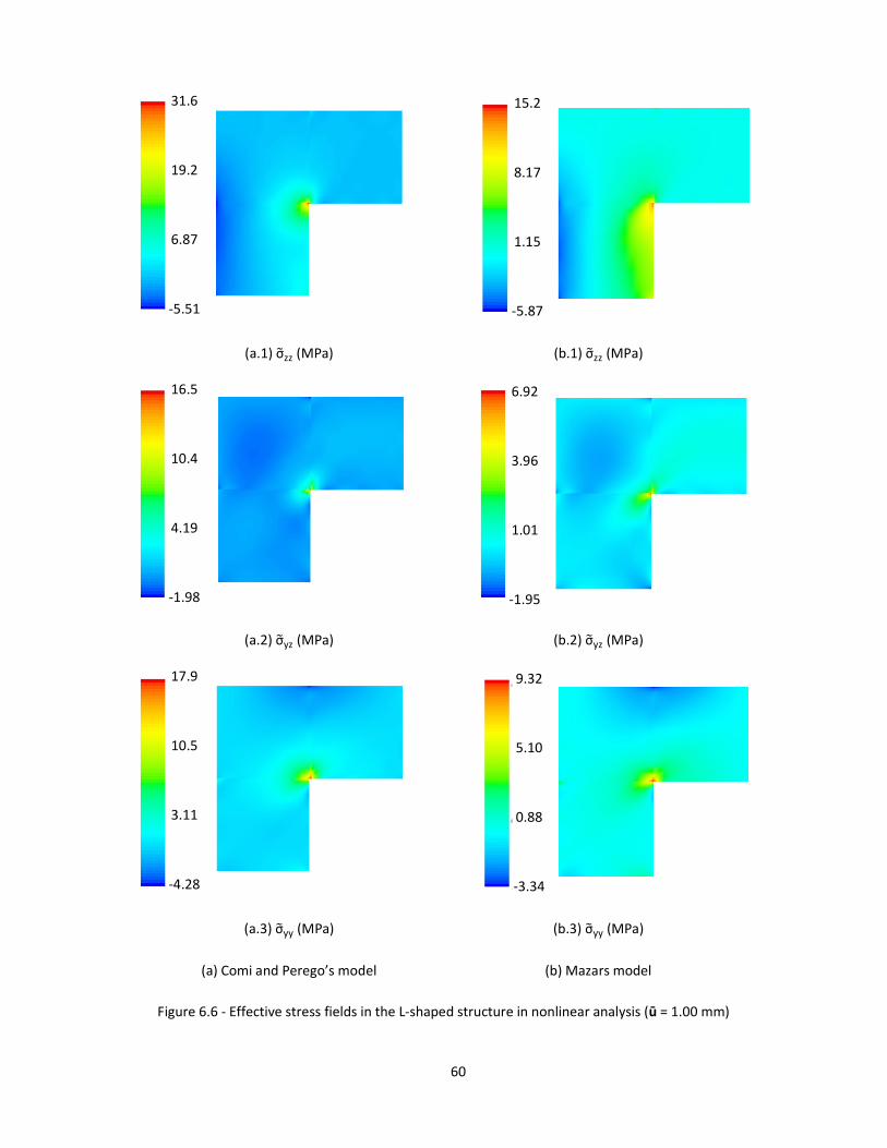
60
(a.1) σzz (MPa) (b.1) σzz (MPa)
(a.2) σyz (MPa) (b.2) σyz (MPa)
(a.3) σyy (MPa) (b.3) σyy (MPa)
(a) Comi and Perego’s model (b) Mazars model
Figure 6.6 - Effective stress fields in the L-shaped structure in nonlinear analysis (ū = 1.00 mm)
31.6
19.2
6.87
-5.51
16.5
10.4
4.19
-1.98
17.9
10.5
3.11
-4.28
15.2
8.17
1.15
-5.87
6.92
3.96
1.01
-1.95
9.32
5.10
0.88
-3.34
61
Figure 6.3 and Figure 6.4 illustrate the evolution of damage, which, as expected, starts in the
area with greater stresses. Inward corners are likely to accumulate higher and more acute stresses
and this formulation appears to be able to model that concentration. The three-dimensional effect is
obvious in Figure 6.3 (b) and Figure6.4 (b), since damage appears in the interior of the structure,
where σxx is more relevant. Moreover, damage also appears in the fixed support, where tensile
stresses are bound to appear. In this point, damage models give distinct results, since Comi and
Perego’s model concentrates damage in the inward corner, while Mazars model spreads damage
from this point to the fixed support. It is important to bear in mind that the nonlocal variables are
different in each model, the elastic energy release rate, Y, and the equivalent strain, ε, respectively.
These responses are clearly an approximation of reality, which seem to give kinematically
admissible solutions, but fail to give a statically admissible solution. The deformed configurations of
the structure and the effective stress fields attest these conclusions. On the one hand, the deformed
configuration depicted in Figure 6.3 and Figure 6.4 induces that the result is kinematically admissible
as the boundaries of adjoining finite elements are still coincident, even though there is in fact a
discrepancy between boundary displacements, which is only perceptible with lower degrees of
approximation and zooming in. On the other hand, the discrepancy between stress fields is
notorious, not only in Figure 6.6, but specially in elastic regime, which is depicted in Figure 6.7, Figure
6.8 and Figure 6.9, with different degrees of approximation. In fact, a conventional way to improve
the solution in basic finite element methodology is to apply an h-refinement or a p-refinement
(except in very particular situations where singularities might lead to numerical instability, in which
case an alternative is to locally enrich the set of approximation functions).
This solution might be seen as a part of a p-refinement, which has the evolution presented in
the following figures, comparing load steps with ū = 0.25 mm, since the lack of equilibrium between
stresses of adjoining elements is more evident in elastic regime. In fact, the high concentration of
stresses in nonlinear regime imposes a scale which masks this divergence if its amplitude is set to
range from the minimum to the maximum stress values. Actually, the realization of the relevance
that the scale amplitude has in all analyses is crucial to come through sound conclusions. For
instance, it is inaccurate to establish that the σyz stress field presents worse compliance between
adjoining elements than the other two unless their scale amplitude is set to be the same. However,
in these tests, the scales always range from the minimum to the maximum value of the displayed
quantity.

62
(a) σzz (MPa) (b) σyz (MPa) (c) σyy (MPa)
Figure 6.7 – Elastic stress diagrams in the L-shaped structure when nv = 4 and ng = 3
(a) σzz (MPa) (b) σyz (MPa) (c) σyy (MPa)
Figure 6.8 – Elastic stress diagrams in the L-shaped structure when nv = 6 and ng = 5
(a) σzz (MPa) (b) σyz (MPa) (c) σyy (MPa)
Figure 6.9 – Elastic stress diagrams in the L-shaped structure when nv = 8 and ng = 7
0.80
0.38
-0.03
-0.44
2.38
1.10
-0.17
-1.45
1.73
0.78
-0.16
-1.11
1.25
0.64
0.03
-0.58
3.28
1.62
-0.04
-1.71
2.36
1.16
-0.03
-1.23
1.76
0.94
0.12
-0.71
4.22
2.21
0.21
-1.80
2.89
1.49
0.09
-1.31
63
This analysis calls attention to two distinct realities. First, as expected, the agreement between
elemental stress fields improves perceptibly with the refinement. Second, stress amplitude is larger
as the degrees of approximation increase. This is coherent with a kinematic solution, which is known
to overestimate the resistance of the structure, which is to say, to underestimate the ultimate load of
the structure and, thus, influence the stresses’ scale too along the loading process.
Another conclusion is that refinement should proceed, in case a better solution is to be
estimated, until the stress values stabilize, without forgetting that the mere look at the scale
amplitude and the colours of the diagrams may be deceiving. In a structure such as this, the inward
corner presents a stress singularity and hence a full convergence is compromised. In these situations
the best thing to do is definitely changing the structure geometry but, considering this is not an
option, a p-refinement provides a valid approach. Unavoidably, achieving better results has its own
costs, since it makes simulation time increase considerably. As a matter of fact, final results with the
lowest degrees of approximation took roughly one fourteenth of the time of the highest.
One final remark goes to the high magnitude effective stresses verified in Figure 6.6. These
values appear because damage is close to its upper bound limit, the unit. In fact, noticing that from
the expressions of chapter 3 also yield
σ = σ
(1 – d) , (6.2)
it is clear that effective stresses go to infinity when damage approaches 1, even with reasonable
stresses, when computed with disregard of the collapse of fibers due to damage (it is the situation of
Figure 3.5). A simple way to burke this situation is to establish a maximum value of the variable
damage in order to have physically more plausible effective stress values, which is, in fact, just
assuming that the stress redistribution capacity in a damaged material has limits. Another way, closer
to the real behavior of concrete is, as mentioned in section 3, to perform a transition to a discrete
crack model, which increases the complexity of the implementation, but benefits its accuracy.
6.3. Analysis of a cantilevered cube under uniform load
This cube is a very simple example of the application of a uniform load in a surface of a three-
dimensional element. Figure 6.10 illustrates this test and Table 6.3 presents complementary
characteristics of the model. Figure 6.11, Figure 6.12 and Figure 6.13 depict some relevant results.

64
(a) geometry of the structure (dimensions in m) (b) coordinate system
Figure 6.10 – Cantilevered cube
Table 6.3 – Relevant characteristics of the cantilevered cube discretization
Geometry of the
structure
Number of elements 1
Number of nodes 8
Number of faces 6
Number of kinematic boundaries 3
Material
properties
Young’s modulus 29200 MPa
Poisson’s ratio 0.2
Characteristic length 0.10 m
Comi and Perego’s
material parameters
k = 5.8 × 10⁻¹⁴ MPa
n = 12 c = 405
Mazars’ material parameters
At = 0.30 Bt = 8000
Ac = 0.85 Bc = 1050
εd0 = 9.34 × 10⁻⁵
Definition of the
approximation
nv 6
ng 5
Number of Lobatto points per
direction per element 20
Governing system Number of degrees of freedom 1137
Load conditions Distributed force (tγγγγ) 2.00 MPa = 2000 kN/m2
Number of load steps 40
1.0
tγγγγ
1.0 1.0
x
z
y
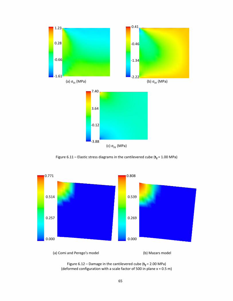
65
(a) σzz (MPa) (b) σyz (MPa)
(c) σyy (MPa)
Figure 6.11 – Elastic stress diagrams in the cantilevered cube (tγγγγ = 1.00 MPa)
(a) Comi and Perego’s model (b) Mazars model
Figure 6.12 – Damage in the cantilevered cube (tγγγγ = 2.00 MPa) (deformed configuration with a scale factor of 500 in plane x = 0.5 m)
0.771
0.514
0.257
0.000
0.41
-0.46
-1.34
-2.22
1.23
0.28
-0.66
-1.61
7.40
3.64
-0.12
-3.88
0.808
0.539
0.269
0.000
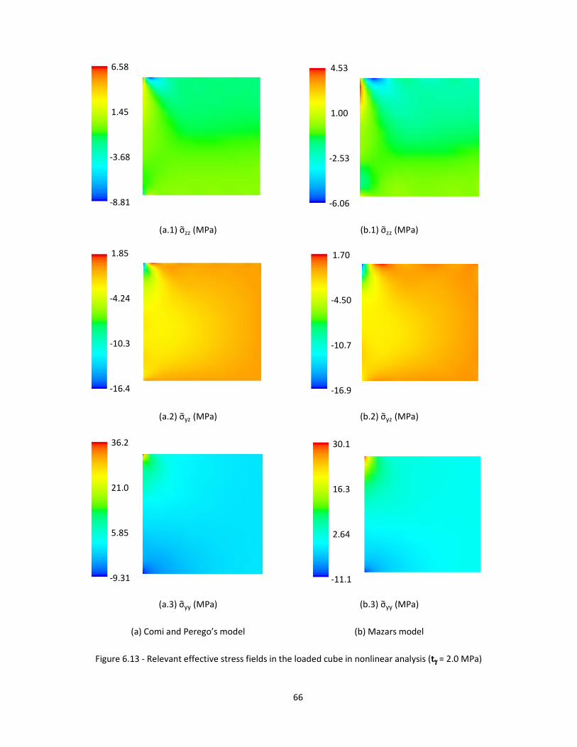
66
(a.1) σzz (MPa) (b.1) σzz (MPa)
(a.2) σyz (MPa) (b.2) σyz (MPa)
(a.3) σyy (MPa) (b.3) σyy (MPa)
(a) Comi and Perego’s model (b) Mazars model
Figure 6.13 - Relevant effective stress fields in the loaded cube in nonlinear analysis (tγγγγ = 2.0 MPa)
6.58
1.45
-3.68
-8.81
1.85
-4.24
-10.3
-16.4
36.2
21.0
5.85
-9.31
4.53
1.00
-2.53
-6.06
30.1
16.3
2.64
-11.1
1.70
-4.50
-10.7
-16.9

67
The results obtained in elastic regime, Figure 6.11, are similar to the classic problem of a
clamped square plate under pure bending, explored in detail by (Meleshko, 1997).
Once damage begins, the parameter calibration presented in section 3.5 seems to yield good
results. As a matter of fact, damage starts at similar load steps. In the case of Comi and Perego’s
model, the first load step in nonlinear regime occurs for a load of 1150 kN/m2, whereas following
Mazars damage model the beginning of damage happens when the load is 1050 kN/m2. Moreover,
the final load step presents similar results, as attested by Figure 6.12 and Figure 6.13, in terms of
damage localization, shape and size of the fracture process zone, maximum value of damage and
stress diagrams. Another way to assess the coherence between models is by comparing their load-
displacement curves. In this case, the load is taken as the distributed force on top of the cube and
the displacement is measured in the middle point of the face opposite to the fixed face of the cube
and taking into account only the vertical component. The result shown in Figure 6.14 proves the
similarity of the results, even though different damage models are used.
Figure 6.14 – Load-displacement curve for the cantilevered cube
6.4. Analysis of a cube with imposed displacement
This example reproduces a cube with one of the faces completely fixed, while the others are
completely free. This cantilevered cube is subject to a uniform displacement of the face opposite to
the fixed one in the direction of the axis that crosses both faces, as depicted in Figure 6.15. Hence,
the major stresses in the structure are tensile. The model’s characteristics are presented in Table 6.4.
0
0.5
1
1.5
2
0 0.04 0.08 0.12 0.16 0.2
u_Mazars
u_Comi
Mazars model
Comi and
Perego model
Load
(M
Pa)
Displacement (mm)
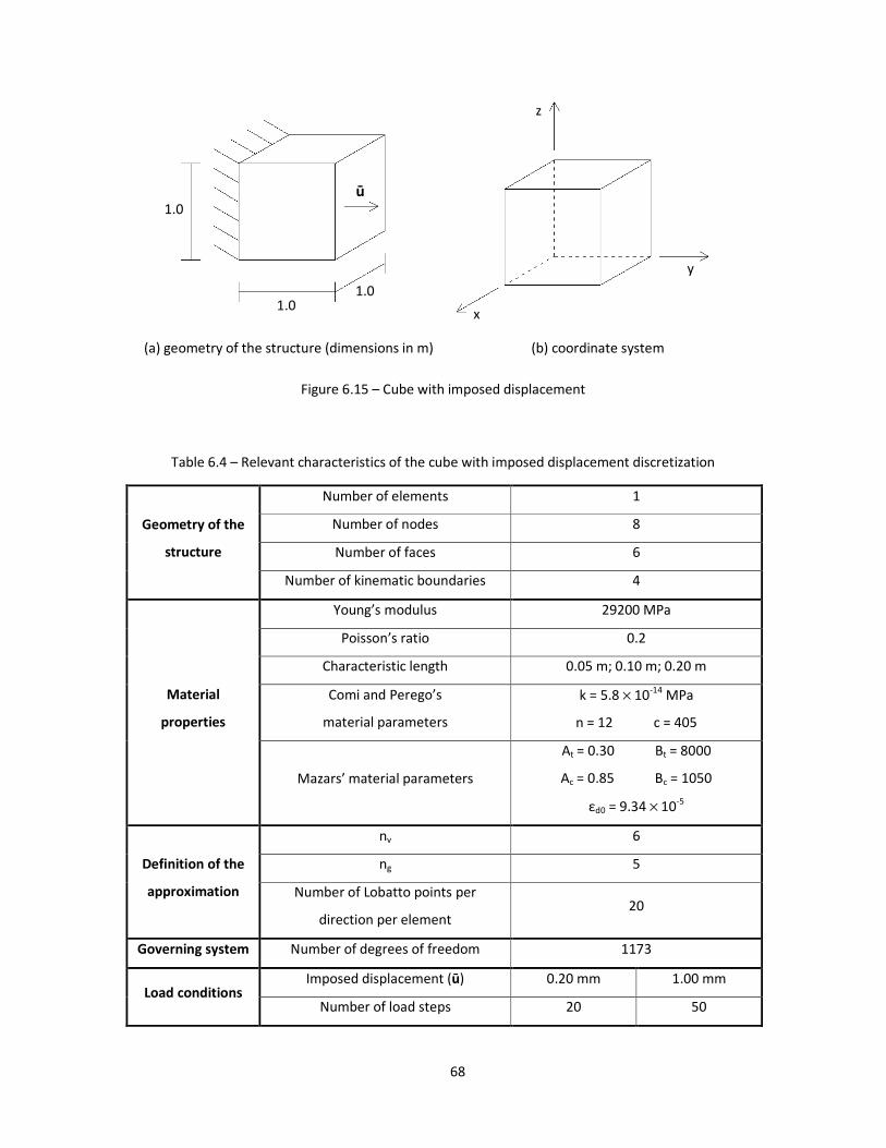
68
(a) geometry of the structure (dimensions in m) (b) coordinate system
Figure 6.15 – Cube with imposed displacement
Table 6.4 – Relevant characteristics of the cube with imposed displacement discretization
Geometry of the
structure
Number of elements 1
Number of nodes 8
Number of faces 6
Number of kinematic boundaries 4
Material
properties
Young’s modulus 29200 MPa
Poisson’s ratio 0.2
Characteristic length 0.05 m; 0.10 m; 0.20 m
Comi and Perego’s
material parameters
k = 5.8 × 10⁻¹⁴ MPa
n = 12 c = 405
Mazars’ material parameters
At = 0.30 Bt = 8000
Ac = 0.85 Bc = 1050
εd0 = 9.34 × 10⁻⁵
Definition of the
approximation
nv 6
ng 5
Number of Lobatto points per
direction per element 20
Governing system Number of degrees of freedom 1173
Load conditions Imposed displacement (ū) 0.20 mm 1.00 mm
Number of load steps 20 50
1.0 ū
1.0 1.0
x
z
y

69
This example is used to illustrate the influence of the characteristic length, l, on the distribution
of damage and, thus, on the size of the fracture process zone.
As expected, independently from the characteristic length, damage is initiated in the vertices of
the fixed face, where stresses in elastic regime are higher, not only σyy but also σyz and σxy due to the
restricted Poisson’s effect. Figure 6.16, Figure 6.17 and Figure 6.18 illustrate these statements.
Figure 6.16 – σyy stress (MPa) in the cube when ū = 0.05 mm (looking at the fixed face)
(a) σyy (MPa) (b) σyz (MPa)
Figure 6.17 – Stress diagrams at plane x = 0.5 m when ū = 0.05 mm
2.39
1.98
1.56
1.14
0.350
0.117
-0.117
-0.350
1.92
1.70
1.48
1.27
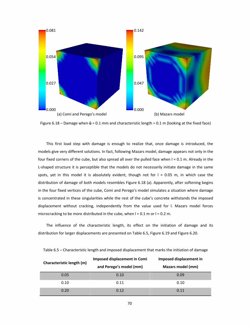
70
(a) Comi and Perego’s model (b) Mazars model
Figure 6.18 – Damage when ū = 0.1 mm and characteristic length = 0.1 m (looking at the fixed face)
This first load step with damage is enough to realize that, once damage is introduced, the
models give very different solutions. In fact, following Mazars model, damage appears not only in the
four fixed corners of the cube, but also spread all over the pulled face when l = 0.1 m. Already in the
L-shaped structure it is perceptible that the models do not necessarily initiate damage in the same
spots, yet in this model it is absolutely evident, though not for l = 0.05 m, in which case the
distribution of damage of both models resembles Figure 6.18 (a). Apparently, after softening begins
in the four fixed vertices of the cube, Comi and Perego’s model simulates a situation where damage
is concentrated in these singularities while the rest of the cube’s concrete withstands the imposed
displacement without cracking, independently from the value used for l. Mazars model forces
microcracking to be more distributed in the cube, when l = 0.1 m or l = 0.2 m.
The influence of the characteristic length, its effect on the initiation of damage and its
distribution for larger displacements are presented on Table 6.5, Figure 6.19 and Figure 6.20.
Table 6.5 – Characteristic length and imposed displacement that marks the initiation of damage
Characteristic length (m) Imposed displacement in Comi
and Perego’s model (mm)
Imposed displacement in
Mazars model (mm)
0.05 0.10 0.09
0.10 0.11 0.10
0.20 0.12 0.11
0.081
0.054
0.027
0.000
0.142
0.095
0.047
0.000
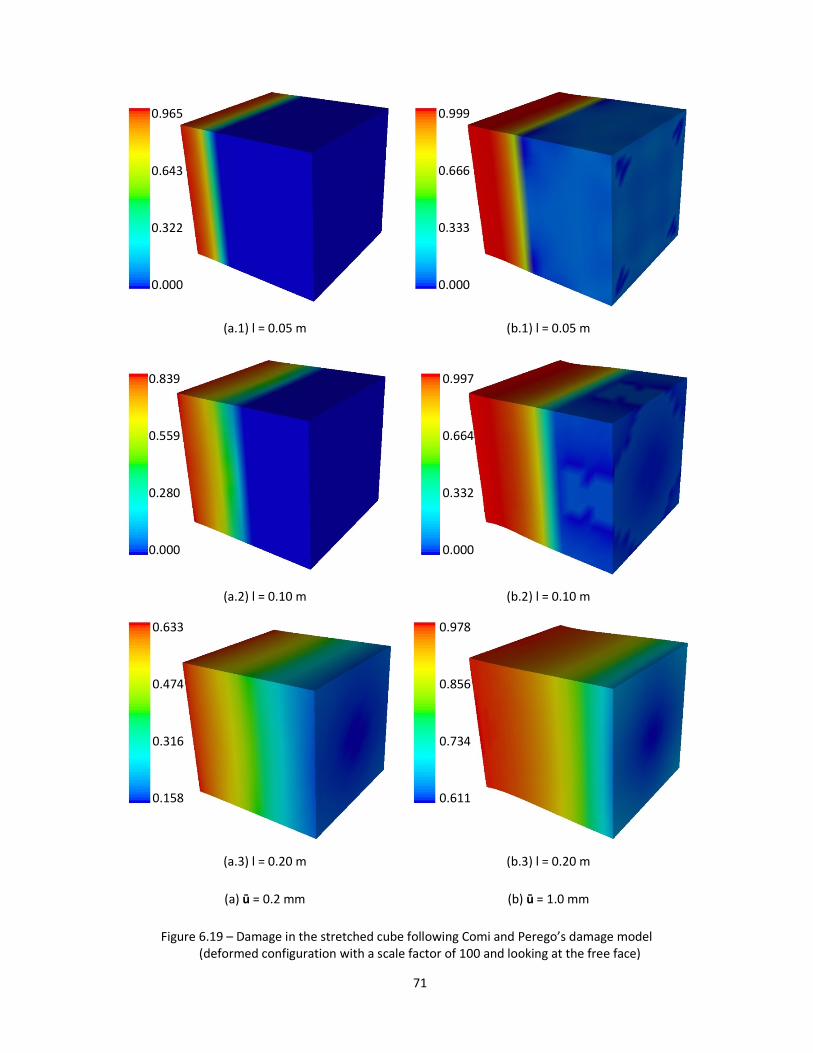
71
(a.1) l = 0.05 m (b.1) l = 0.05 m
(a.2) l = 0.10 m (b.2) l = 0.10 m
(a.3) l = 0.20 m (b.3) l = 0.20 m
(a) ū = 0.2 mm (b) ū = 1.0 mm
Figure 6.19 – Damage in the stretched cube following Comi and Perego’s damage model (deformed configuration with a scale factor of 100 and looking at the free face)
0.965
0.643
0.322
0.000
0.839
0.559
0.280
0.000
0.633
0.474
0.316
0.158
0.999
0.666
0.333
0.000
0.997
0.664
0.332
0.000
0.978
0.856
0.734
0.611
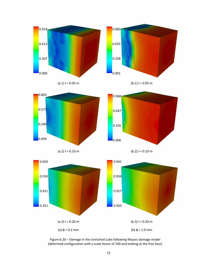
72
(a.1) l = 0.05 m (b.1) l = 0.05 m
(a.2) l = 0.10 m (b.2) l = 0.10 m
(a.3) l = 0.20 m (b.3) l = 0.20 m
(a) ū = 0.2 mm (b) ū = 1.0 mm
Figure 6.20 – Damage in the stretched cube following Mazars damage model (deformed configuration with a scale factor of 100 and looking at the free face)
0.919
0.613
0.307
0.000
0.863
0.577
0.290
0.004
0.983
0.655
0.328
0.001
0.968
0.647
0.326
0.006
0.941
0.934
0.927
0.920
0.650
0.550
0.451
0.351

73
The sensitivity of the model to the value of the characteristic length is hereby presented. In both
models, when l = 0.05 m, most of the cube is intact and, hence, the highest concentrations of
damage occur, since the behaviour of the structure is closer to local as shown in Figure 6.19 (a) and
Figure 6.20 (a). On the other hand, l = 0.20 m leads to damage in the entire cube with a much
smoother distribution, which is hardly realistic in case of a quasibrittle behaviour such as concrete’s.
Apart from these considerations, the results are coherent with the fact that, when the characteristic
length is smaller, the fracture process zone is narrower for similar values of damage. Nevertheless,
the two models give very distinct results when it comes to the localization of damage. The fact that
the distribution of strains and stresses in elastic regime is rather homogeneous and that the
maximum and minimum values occur close to each other at the fixe face may explain that, after
regularization is applied, the nonlocal variables of each model have an even more homogeneous
distribution. However, while the nonlocal elastic energy release rate is higher in the fixed face, the
nonlocal equivalent strain has its greatest values at the free face. Anyway, it might not be reasonable
to assume that plain concrete is able to distribute damage as smoothly as when the characteristic
length is taken with the largest value presented (Figure 6.19(a3) and Figure 6.20(a3)). Moreover, it is
straightforward that too high effective stresses appear with damage as close to the unit as when the
characteristic length is very short (Figure 6.19 (a1) and Figure 6.20 (a1)), which represents a situation
unlikely to have a physical meaning and, once again, leads to the relevance of introducing crack
models as a complement to continuum damage models. An illustration of the discrepancy of the
effective stresses obtained with different values for parameter l is given in Figure 6.21.
(a) l = 0.05 m (b) l = 0.20 m
Figure 6.21 – Effective σyy (MPa) for ū = 0.2 mm with Comi and Perego’s model
(looking at the fixed face)
59.3
39.5
19.7
-0.07
13.1
9.94
6.76
3.58
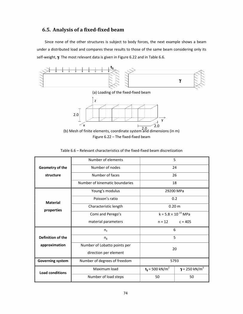
74
6.5. Analysis of a fixed-fixed beam
Since none of the other structures is subject to body forces, the next example shows a beam
under a distributed load and compares these results to those of the same beam considering only its
self-weight, γγγγ. The most relevant data is given in Figure 6.22 and in Table 6.6.
(a) Loading of the fixed-fixed beam
(b) Mesh of finite elements, coordinate system and dimensions (in m)
Figure 6.22 – The fixed-fixed beam
Table 6.6 – Relevant characteristics of the fixed-fixed beam discretization
Geometry of the
structure
Number of elements 5
Number of nodes 24
Number of faces 26
Number of kinematic boundaries 18
Material
properties
Young’s modulus 29200 MPa
Poisson’s ratio 0.2
Characteristic length 0.20 m
Comi and Perego’s
material parameters
k = 5.8 × 10⁻¹⁴ MPa
n = 12 c = 405
Definition of the
approximation
nv 6
ng 5
Number of Lobatto points per
direction per element 20
Governing system Number of degrees of freedom 5793
Load conditions Maximum load tγγγγ = 500 kN/m2 γγγγ = 250 kN/m3
Number of load steps 50 50
γγγγ
tγγγγ
2.0
2.0 2.0 x
z
y
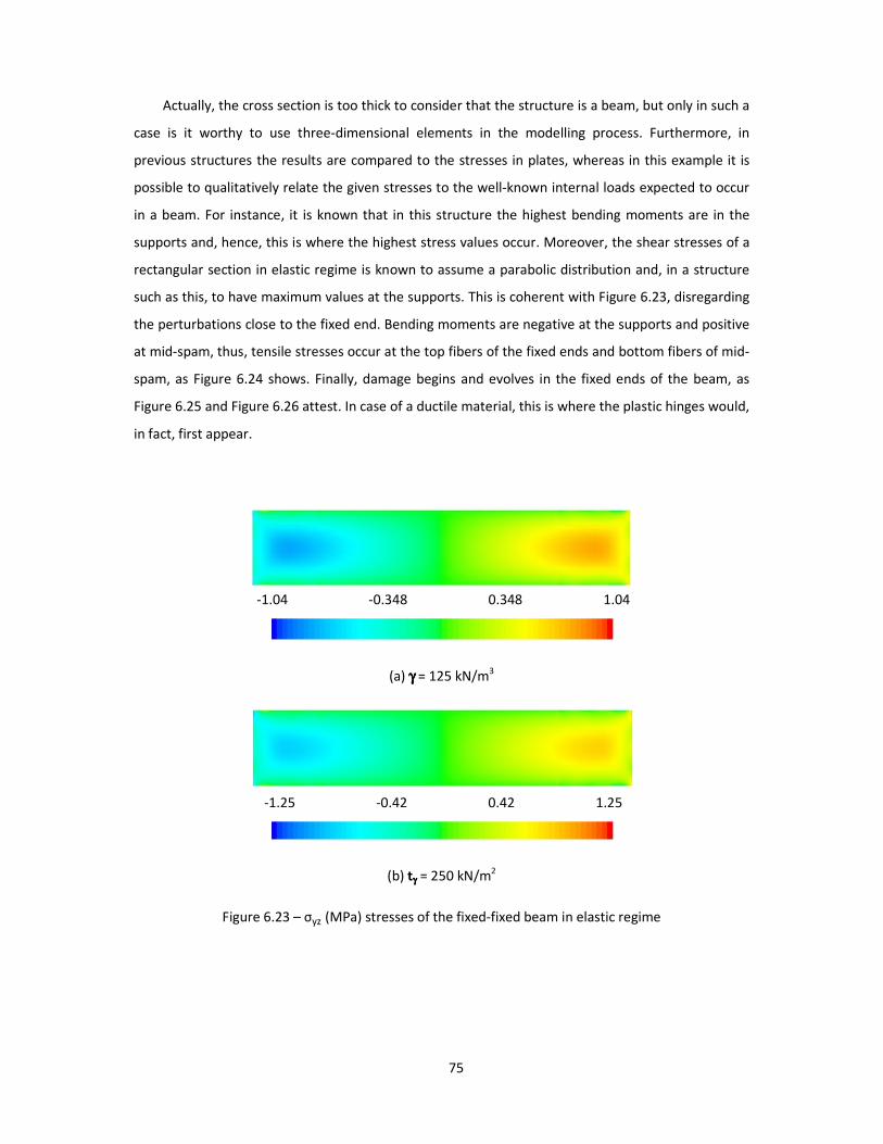
75
Actually, the cross section is too thick to consider that the structure is a beam, but only in such a
case is it worthy to use three-dimensional elements in the modelling process. Furthermore, in
previous structures the results are compared to the stresses in plates, whereas in this example it is
possible to qualitatively relate the given stresses to the well-known internal loads expected to occur
in a beam. For instance, it is known that in this structure the highest bending moments are in the
supports and, hence, this is where the highest stress values occur. Moreover, the shear stresses of a
rectangular section in elastic regime is known to assume a parabolic distribution and, in a structure
such as this, to have maximum values at the supports. This is coherent with Figure 6.23, disregarding
the perturbations close to the fixed end. Bending moments are negative at the supports and positive
at mid-spam, thus, tensile stresses occur at the top fibers of the fixed ends and bottom fibers of mid-
spam, as Figure 6.24 shows. Finally, damage begins and evolves in the fixed ends of the beam, as
Figure 6.25 and Figure 6.26 attest. In case of a ductile material, this is where the plastic hinges would,
in fact, first appear.
(a) γγγγ = 125 kN/m3
(b) tγγγγ = 250 kN/m2
Figure 6.23 – σyz (MPa) stresses of the fixed-fixed beam in elastic regime
-1.04 -0.348 0.348 1.04
-1.25 -0.42 0.42 1.25
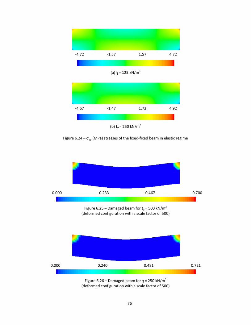
76
(a) γγγγ = 125 kN/m3
(b) tγγγγ = 250 kN/m2
Figure 6.24 – σyy (MPa) stresses of the fixed-fixed beam in elastic regime
Figure 6.25 – Damaged beam for tγγγγ = 500 kN/m2 (deformed configuration with a scale factor of 500)
Figure 6.26 – Damaged beam for γγγγ = 250 kN/m3 (deformed configuration with a scale factor of 500)
-4.72 -1.57 1.57 4.72
-4.67 -1.47 1.72 4.92
0.000 0.233 0.467 0.700
0.000 0.240 0.481 0.721
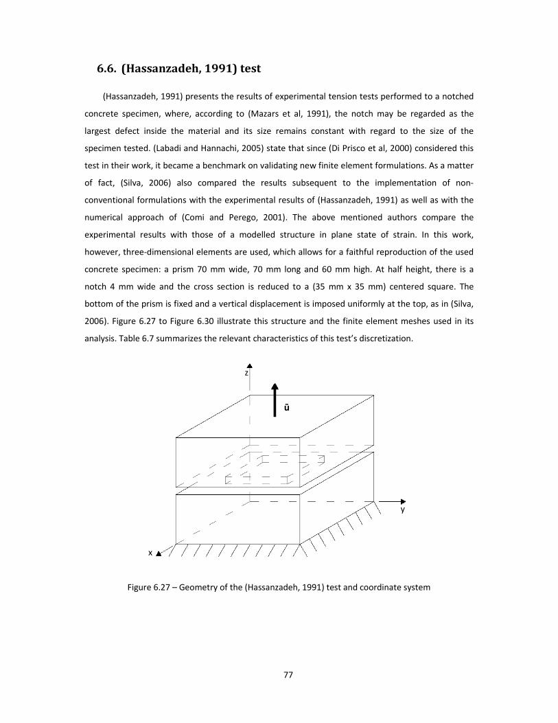
77
6.6. (Hassanzadeh, 1991) test
(Hassanzadeh, 1991) presents the results of experimental tension tests performed to a notched
concrete specimen, where, according to (Mazars et al, 1991), the notch may be regarded as the
largest defect inside the material and its size remains constant with regard to the size of the
specimen tested. (Labadi and Hannachi, 2005) state that since (Di Prisco et al, 2000) considered this
test in their work, it became a benchmark on validating new finite element formulations. As a matter
of fact, (Silva, 2006) also compared the results subsequent to the implementation of non-
conventional formulations with the experimental results of (Hassanzadeh, 1991) as well as with the
numerical approach of (Comi and Perego, 2001). The above mentioned authors compare the
experimental results with those of a modelled structure in plane state of strain. In this work,
however, three-dimensional elements are used, which allows for a faithful reproduction of the used
concrete specimen: a prism 70 mm wide, 70 mm long and 60 mm high. At half height, there is a
notch 4 mm wide and the cross section is reduced to a (35 mm x 35 mm) centered square. The
bottom of the prism is fixed and a vertical displacement is imposed uniformly at the top, as in (Silva,
2006). Figure 6.27 to Figure 6.30 illustrate this structure and the finite element meshes used in its
analysis. Table 6.7 summarizes the relevant characteristics of this test’s discretization.
Figure 6.27 – Geometry of the (Hassanzadeh, 1991) test and coordinate system
x
z
y
ū
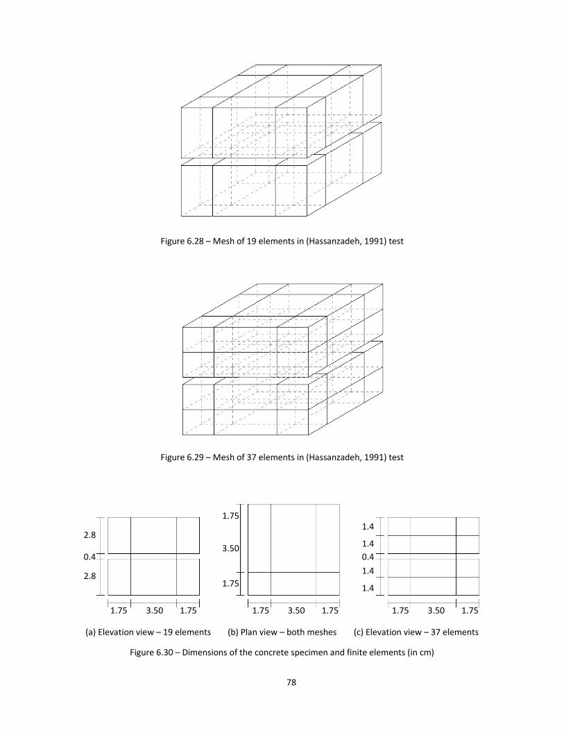
78
Figure 6.28 – Mesh of 19 elements in (Hassanzadeh, 1991) test
Figure 6.29 – Mesh of 37 elements in (Hassanzadeh, 1991) test
(a) Elevation view – 19 elements (b) Plan view – both meshes (c) Elevation view – 37 elements
Figure 6.30 – Dimensions of the concrete specimen and finite elements (in cm)
1.75 3.50 1.75 1.75 3.50 1.75 1.75 3.50 1.75
2.8
2.8
0.4 0.4
1.4
1.4
1.4
1.4
1.75
1.75
3.50
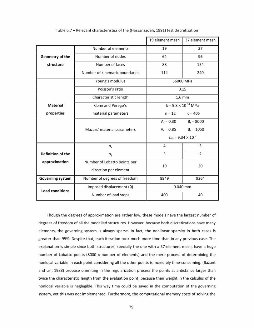
79
Table 6.7 – Relevant characteristics of the (Hassanzadeh, 1991) test discretization
19 element mesh 37 element mesh
Geometry of the
structure
Number of elements 19 37
Number of nodes 64 96
Number of faces 88 154
Number of kinematic boundaries 114 240
Material
properties
Young’s modulus 36000 MPa
Poisson’s ratio 0.15
Characteristic length 1.6 mm
Comi and Perego’s
material parameters
k = 5.8 × 10⁻¹⁴ MPa
n = 12 c = 405
Mazars’ material parameters
At = 0.30 Bt = 8000
Ac = 0.85 Bc = 1050
εd0 = 9.34 × 10⁻⁵
Definition of the
approximation
nv 4 3
ng 3 2
Number of Lobatto points per
direction per element 10 20
Governing system Number of degrees of freedom 8949 9264
Load conditions Imposed displacement (ū) 0.040 mm
Number of load steps 400 40
Though the degrees of approximation are rather low, these models have the largest number of
degrees of freedom of all the modelled structures. However, because both discretizations have many
elements, the governing system is always sparse. In fact, the nonlinear sparsity in both cases is
greater than 95%. Despite that, each iteration took much more time than in any previous case. The
explanation is simple since both structures, specially the one with a 37-element mesh, have a huge
number of Lobatto points (8000 × number of elements) and the mere process of determining the
nonlocal variable in each point considering all the other points is incredibly time-consuming. (Bažant
and Lin, 1988) propose ommiting in the regularization process the points at a distance larger than
twice the characteristic length from the evaluation point, because their weight in the calculus of the
nonlocal variable is neglegible. This way time could be saved in the computation of the governing
system, yet this was not implemented. Furthermore, the computational memory costs of solving the
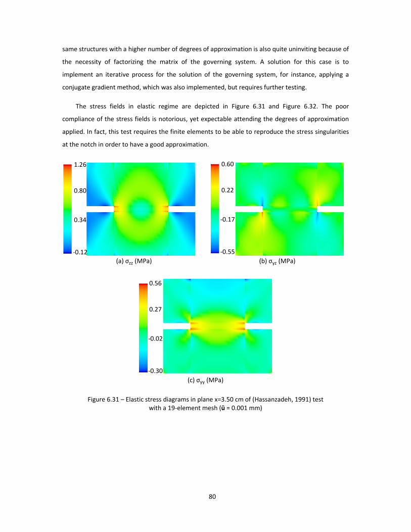
80
same structures with a higher number of degrees of approximation is also quite uninviting because of
the necessity of factorizing the matrix of the governing system. A solution for this case is to
implement an iterative process for the solution of the governing system, for instance, applying a
conjugate gradient method, which was also implemented, but requires further testing.
The stress fields in elastic regime are depicted in Figure 6.31 and Figure 6.32. The poor
compliance of the stress fields is notorious, yet expectable attending the degrees of approximation
applied. In fact, this test requires the finite elements to be able to reproduce the stress singularities
at the notch in order to have a good approximation.
(a) σzz (MPa) (b) σyz (MPa)
(c) σyy (MPa)
Figure 6.31 – Elastic stress diagrams in plane x=3.50 cm of (Hassanzadeh, 1991) test with a 19-element mesh (ū = 0.001 mm)
0.60
0.22
-0.17
-0.55
1.26
0.80
0.34
-0.12
0.56
0.27
-0.02
-0.30
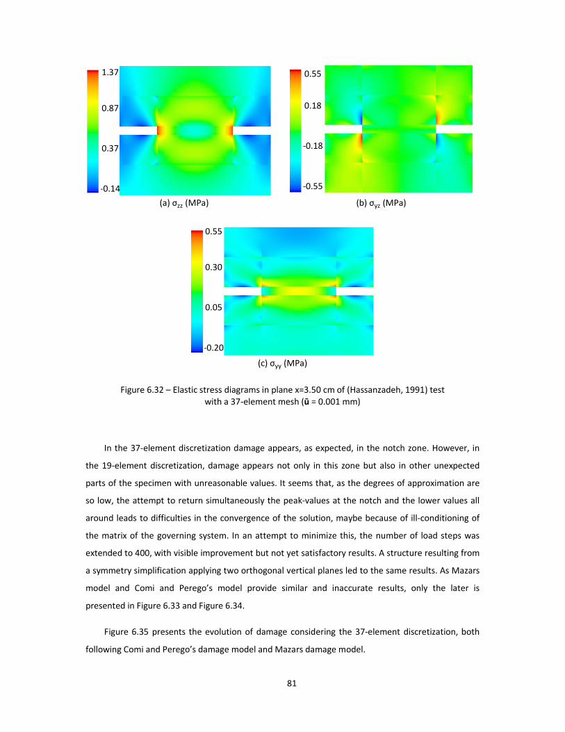
81
(a) σzz (MPa) (b) σyz (MPa)
(c) σyy (MPa)
Figure 6.32 – Elastic stress diagrams in plane x=3.50 cm of (Hassanzadeh, 1991) test with a 37-element mesh (ū = 0.001 mm)
In the 37-element discretization damage appears, as expected, in the notch zone. However, in
the 19-element discretization, damage appears not only in this zone but also in other unexpected
parts of the specimen with unreasonable values. It seems that, as the degrees of approximation are
so low, the attempt to return simultaneously the peak-values at the notch and the lower values all
around leads to difficulties in the convergence of the solution, maybe because of ill-conditioning of
the matrix of the governing system. In an attempt to minimize this, the number of load steps was
extended to 400, with visible improvement but not yet satisfactory results. A structure resulting from
a symmetry simplification applying two orthogonal vertical planes led to the same results. As Mazars
model and Comi and Perego’s model provide similar and inaccurate results, only the later is
presented in Figure 6.33 and Figure 6.34.
Figure 6.35 presents the evolution of damage considering the 37-element discretization, both
following Comi and Perego’s damage model and Mazars damage model.
0.55
0.30
0.05
-0.20
0.55
0.18
-0.18
-0.55
1.37
0.87
0.37
-0.14
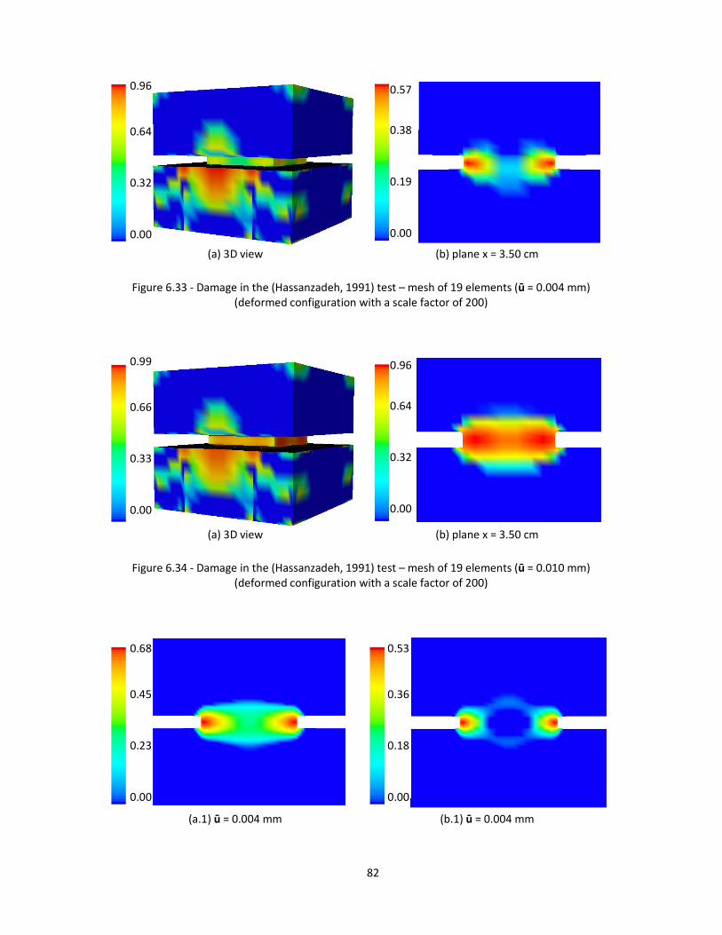
82
(a) 3D view (b) plane x = 3.50 cm
Figure 6.33 - Damage in the (Hassanzadeh, 1991) test – mesh of 19 elements (ū = 0.004 mm) (deformed configuration with a scale factor of 200)
(a) 3D view (b) plane x = 3.50 cm
Figure 6.34 - Damage in the (Hassanzadeh, 1991) test – mesh of 19 elements (ū = 0.010 mm) (deformed configuration with a scale factor of 200)
(a.1) ū = 0.004 mm (b.1) ū = 0.004 mm
0.57
0.38
0.19
0.00
0.96
0.64
0.32
0.00
0.96
0.64
0.32
0.00
0.99
0.66
0.33
0.00
0.68
0.45
0.23
0.00
0.53
0.36
0.18
0.00
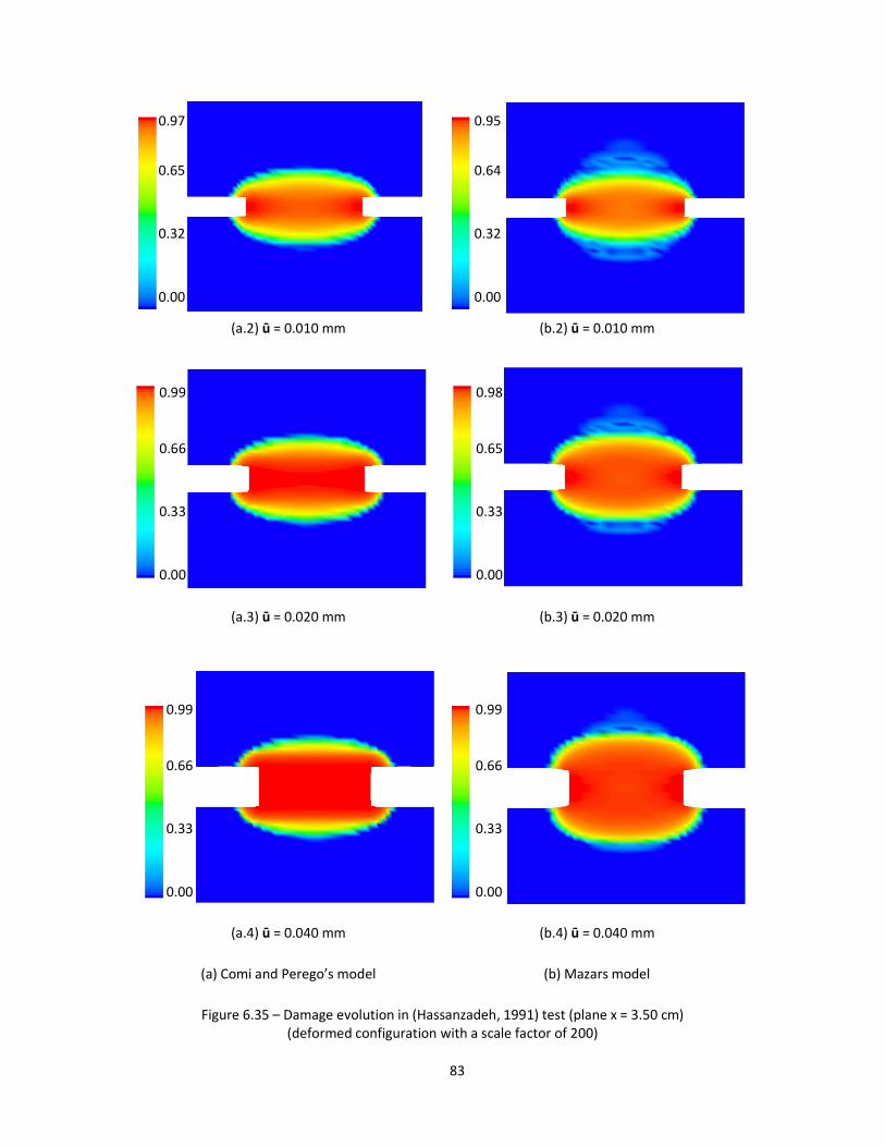
83
(a.2) ū = 0.010 mm (b.2) ū = 0.010 mm
(a.3) ū = 0.020 mm (b.3) ū = 0.020 mm
(a.4) ū = 0.040 mm (b.4) ū = 0.040 mm
(a) Comi and Perego’s model (b) Mazars model
Figure 6.35 – Damage evolution in (Hassanzadeh, 1991) test (plane x = 3.50 cm) (deformed configuration with a scale factor of 200)
0.97
0.65
0.32
0.00
0.99
0.66
0.33
0.00
0.99
0.66
0.33
0.00
0.95
0.64
0.32
0.00
0.98
0.65
0.33
0.00
0.99
0.66
0.33
0.00
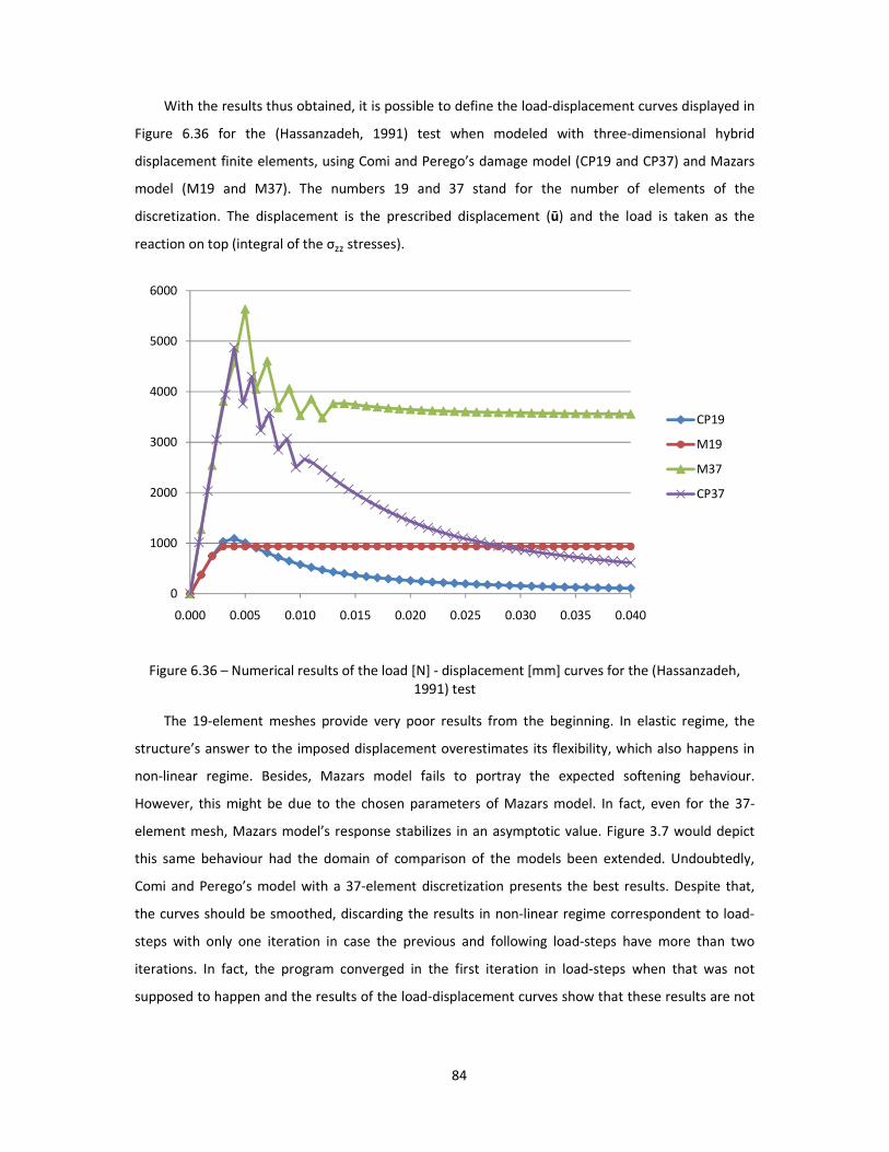
84
With the results thus obtained, it is possible to define the load-displacement curves displayed in
Figure 6.36 for the (Hassanzadeh, 1991) test when modeled with three-dimensional hybrid
displacement finite elements, using Comi and Perego’s damage model (CP19 and CP37) and Mazars
model (M19 and M37). The numbers 19 and 37 stand for the number of elements of the
discretization. The displacement is the prescribed displacement (ū) and the load is taken as the
reaction on top (integral of the σzz stresses).
Figure 6.36 – Numerical results of the load [N] - displacement [mm] curves for the (Hassanzadeh, 1991) test
The 19-element meshes provide very poor results from the beginning. In elastic regime, the
structure’s answer to the imposed displacement overestimates its flexibility, which also happens in
non-linear regime. Besides, Mazars model fails to portray the expected softening behaviour.
However, this might be due to the chosen parameters of Mazars model. In fact, even for the 37-
element mesh, Mazars model’s response stabilizes in an asymptotic value. Figure 3.7 would depict
this same behaviour had the domain of comparison of the models been extended. Undoubtedly,
Comi and Perego’s model with a 37-element discretization presents the best results. Despite that,
the curves should be smoothed, discarding the results in non-linear regime correspondent to load-
steps with only one iteration in case the previous and following load-steps have more than two
iterations. In fact, the program converged in the first iteration in load-steps when that was not
supposed to happen and the results of the load-displacement curves show that these results are not
0
1000
2000
3000
4000
5000
6000
0.000 0.005 0.010 0.015 0.020 0.025 0.030 0.035 0.040
CP19
M19
M37
CP37
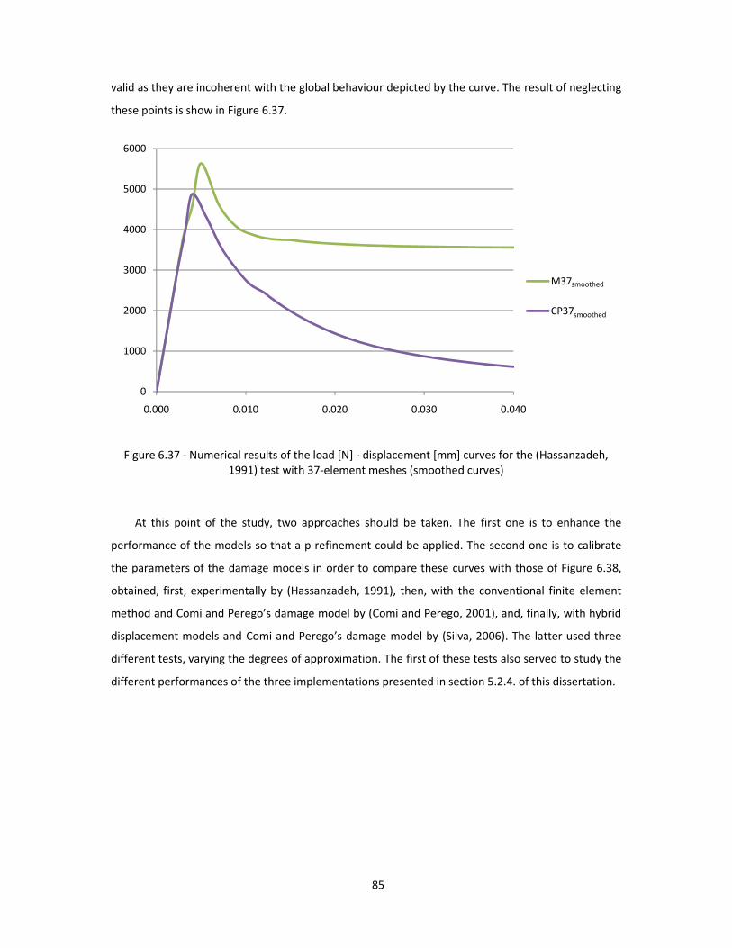
85
valid as they are incoherent with the global behaviour depicted by the curve. The result of neglecting
these points is show in Figure 6.37.
Figure 6.37 - Numerical results of the load [N] - displacement [mm] curves for the (Hassanzadeh, 1991) test with 37-element meshes (smoothed curves)
At this point of the study, two approaches should be taken. The first one is to enhance the
performance of the models so that a p-refinement could be applied. The second one is to calibrate
the parameters of the damage models in order to compare these curves with those of Figure 6.38,
obtained, first, experimentally by (Hassanzadeh, 1991), then, with the conventional finite element
method and Comi and Perego’s damage model by (Comi and Perego, 2001), and, finally, with hybrid
displacement models and Comi and Perego’s damage model by (Silva, 2006). The latter used three
different tests, varying the degrees of approximation. The first of these tests also served to study the
different performances of the three implementations presented in section 5.2.4. of this dissertation.
0
1000
2000
3000
4000
5000
6000
0.000 0.010 0.020 0.030 0.040
M37
CP37
smoothed
smoothed
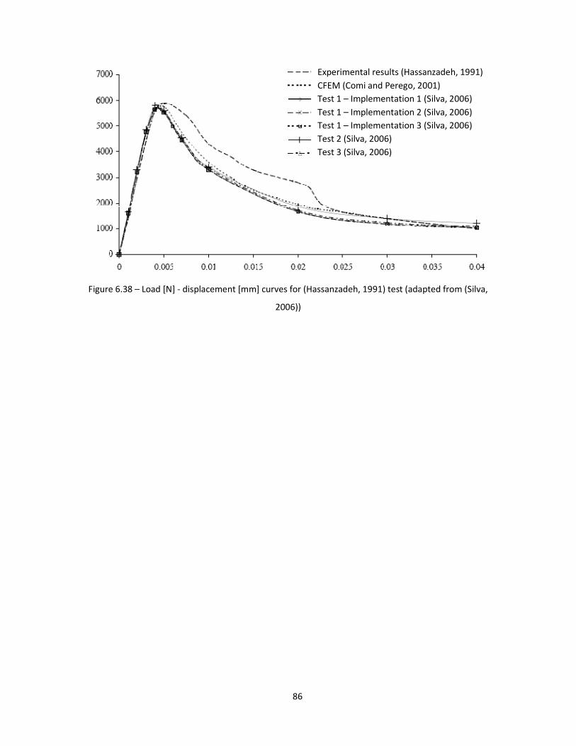
86
Figure 6.38 – Load [N] - displacement [mm] curves for (Hassanzadeh, 1991) test (adapted from (Silva,
2006))
Experimental results (Hassanzadeh, 1991)
CFEM (Comi and Perego, 2001)
Test 1 – Implementation 1 (Silva, 2006)
Test 1 – Implementation 2 (Silva, 2006)
Test 1 – Implementation 3 (Silva, 2006)
Test 2 (Silva, 2006)
Test 3 (Silva, 2006)

87
7. Conclusions and further developments
7.1. Conclusions
Finite element methods are broadly used in software for structural analysis and design. The
demands of structural engineering are answered by a vast diversity of options, modelling columns or
beams, slabs or plates, concrete or steel, simple or complex structures under static or dynamics
loads. However, the leap to nonlinear analysis is rarely taken. For instance, in case of a seismic
analysis, Eurocode 8 advises to take advantage of the structure’s ductility. However, this is done
always in linear elastic analysis, just by adding a behaviour coefficient to correct the data. As (Lopes
et al, 2008) explain, the need of making this a safe procedure restricts the use of accurate values, for
the sake of simplicity. However, if the nonlinear behaviour of the structures was modelled in an
efficient way, this kind of analysis would be more accurate and, hence, structural design would be
improved.
Continuum damage mechanics provides a robust framework to model the nonlinear behaviour
of materials, namely concrete. Besides, its versatility allows the derivation of different damage
models, which plays an important role in this dissertation since two models are applied and, thus, the
coherence between their results underlines that the implementations are fit to analyse three-
dimensional structures considering their physically nonlinear behaviour.

88
In order to develop an efficient three-dimensional hybrid displacement model for physically
nonlinear analysis of concrete, some approaches were taken:
1. An analytical expression for the integration of the product of the derivatives of Legendre
polynomials was deduced. Thus, a linear elastic analysis of the structure is possible without
numerical integration and, hence, without defining a mesh of integration points. Simulations
are faster and more accurate in elastic regime.
2. Two different damage models with totally independent subroutines were implemented,
endorsing each other’s results.
3. Two different implementations were tested. The first one derives directly from the concept
of damage as a measure of the loss of stiffness and, hence, implies the existence of a
nonlinear generalized stiffness operator that must be recomputed at each iteration of each
load step. Since this matrix turns from being sparse to being potentially full, the second type
of implementation is an attempt to avoid this unwieldy process by introducing damage in a
corrective term on the right-hand-side. The second implementation needs further testing
before being presented.
4. Two processes were applied to solve the governing system. The first is the direct process,
which needs to factorize the governing matrix and, hence, has high computational costs. The
second subroutine applies the conjugate gradient method to solve iteratively the system,
but, unless the dimensions of the governing matrix are very high, this time-consuming
approach is not an interesting option.
All in all, this work integrates a major project with another non-conventional formulation also
being developed with the same purpose of modelling the physically nonlinear behaviour of concrete,
the hybrid-mixed stress formulation. (Silva, 2006) states that the hybrid displacement models have a
slightly easier and more intuitive implementation than other non-conventional formulations.
Nonetheless, the hybrid-mixed stress formulation is likely to draw a larger concentration of efforts
for this is truly a disruptive approach on finite element analysis because its aim is to find statically
admissible solutions. In fact, even considering the formulations to be tantamount to each other in
mathematical terms, meaning that they require approximately the same computational effort to
achieve reasonable results, while the hybrid displacement model returns a good solution in terms of
compatibility, appealing only if the objective is to draw the deformed configuration of the structure,
the hybrid-mixed stress approach leads to a solution which is bound to be in equilibrium and, hence,
renders more credible stress diagrams. Assuming a strictly numerical point of view, it would be
indifferent whether the given solution is an upper bound or a lower bound, as long as the
89
convergence rate is satisfactory. However, in terms of structural analysis, that means the difference
between enduring and collapsing.
Nevertheless, in the real world, there are no straight lines or perfect curves, no homogeneous
materials up to infinitesimal level or foolproof constitutive relations, no uniform quasi-static loadings
or approximation functions. Engineers have to deal with that in every project, establishing dimension
tolerances, quality patterns of the materials, and service and ultimate loads for structures according
to their expected lifetime, not to mention the mandatory safety factors. Once this is assumed, it is
also clear that structure analysis provides approximated solutions based on approximated data.
Assumptions have to be made at each step with one fundamental guideline: to preserve the accuracy
of the results as much as possible in balance with the efficiency of the algorithms. Therefore,
accepting the limitations regarding the fact that the model focuses on providing solutions respecting
the kinematic conditions and considering the fairly sound results obtained in chapter 6, the key-
conclusion of this work is that hybrid displacement models provide reliable results under a diverse
number of circumstances. However, some drawbacks are not easy to cap. In fact, the lack of
intuitiveness associated with the models is not appealing, but this should not compromise the
generalized use of alternatives to the conventional finite element method if they are more efficient.
The greatest problem is undoubtedly the computational cost of the model. In fact, the three-
dimensional simulation of a complex structure is far from being attainable in a short period of time if
damage occurs.
7.2. Further developments
The developed models successfully introduce damage in the three-dimensional hybrid
displacement formulation. Further developments concern both overcoming presented limitations
and extending the application field of this formulation. Among others:
1. Parallel processing would decrease the simulation time considerably.
2. Limiting the considered neighbourhood of each point when applying the regularization
method decreases the simulation time, even though conceptually it is not as correct as the
implemented version. Nevertheless, in practical terms the results might be nearly the same.
3. The applied convergence method is a secant method. It might be useful to compare its
performance with others which take less iterations to reach convergence. In fact, the secant

90
method would be more adequate if computing the governing system was not as time-
consuming as it is even in simple examples as the presented in this dissertation.
4. The developed program should be able to model finite elements with geometrical shapes
other than rectangular prisms, namely, any kind of cuboids and solids with curve faces. The
first case is rather easy, since the only additional difficulty is that the Jacobian of the
coordinate transformation from the parent element to the global coordinate system is not
constant. Elements with curved faces require not only what is mentioned above, but also a
greater number of nodes to detail the structure.
5. The development and optimization of the implementation which introduces damage as a
corrective term on the right-hand-side of the governing system might be profitable. Besides,
the improvement of the iterative process of solving the governing system with the conjugate
gradient method might allow the use of h-refinements and p-refinements in the studied
structures without unreasonable computational memory costs.
6. The introduction of different damage models may yield more accurate results, namely if the
models consider irreversible strains when unloading is foreseen.
7. The most demanding development is probably to implement a unified framework for
continuum damage and fracture mechanics, able to model the initial diffuse microcracking
of concrete and the coalescent macrocracks that appear as damage develops.
What better way to finish a work than realising that the travelled path led to the very
beginning? However, even though it all starts with several questions, some objectives and very few
answers, in the end that first blurred view of the problem expressed through Professor Zienkiewicz’s
words “At all stages of the development of numerical methodology by engineers, the achievement
of practical results is paramount.” (Zienkiewicz, 2001) is replaced by more questions and different
goals, as well as, thankfully, several answers and the accomplishment of the preceding objectives.
Moreover, the next few lines of (Zienkiewicz, 2001) are also worthy of quoting, once it is now clear
that they are perfectly consonant with the work developed along this dissertation: “Although many
solutions concentrated on purely linear problems (...), much of the real behaviour is non-linear and
complex. For this reason the interaction between the development of theory and the development
of computation has occupied much effort.”. For this reason also, as a conclusion of all that has been
written about the subject of non-conventional finite element formulations, the potential of these
methods is being uncovered as more powerful computational tools appear and with the effort of
many researchers. This work joins others in the purpose of widening the application fields of these
formulations so that a thorough study of the advantages that they provide to structural mechanics is
more extensively recognized in the world of structural engineering.

91

92
93
References
Bascoul, A. (1996). State of the art report - Part 2: Mechanical micro-cracking of concrete. Matériaux
et Constructions/Materials and Structures , 29, 66-78.
Bažant, Z. P. (1984). Imbricate continuum and progressive fracturing of concrete and geomaterials.
Meccanica , 14, 86-93.
Bažant, Z. P. and Lin, F.-B. (1988). Nonlocal Smeared Cracking Model for Concrete Fracture. Journal of
Structural Engineering , 114, nº. 11, 2493-2510.
Bažant, Z. P. and Pang, S. D. (2006). Statistical mechanics of safety factors and size effect in
quasibrittle fracture - Fracture of Nano and Engineering Materials and Structures. Springer
Netherlands.
Bažant, Z. P. and Pijaudier-Cabot, G. (1988). Nonlocal continuum damage, localization instability and
convergence. Journal of Applied Mechanics , 55 (June), 287-293.
Beyer, W. H. (1987). CRC Standard Mathematical Tables. CRC Press, Boca Raton.
Borino, G. and De Borst, R. (2000). Some observations on the regularizing field for gradient damage
models. Acta Mechanica , 140, 149-162.
Chow, C. and Wang, J. (1987). An anisotropic theory of elasticity for continuum damage mechanics.
International Journal of Fracture , 33, 3-16.
Comi, C. and Perego, U. (2001). Nonlocal aspects of nonlocal damage analyses of concrete strucutres.
European Journal of Finite Elements , 10, 227–242.
Comi, C., Mariani, S. and Perego, U. (2002). On the transition from continuum nonlocal damage to
quasi-brittle discrete crack models. Third Joint Conference of Italian Group of Computational
Mechanics and Ibero-Latin American Association of Computational Methods in Engineering .
De Borst, R. and Guitiérrez, M. A. (1999). A unified framework for concrete damage and fracture
models including size effects. International Journal of Fracture , 95, 261-277.
Di Prisco, M., Ferrara, L., Meftah, F., de Borst, R., Mazars, J. and Reynouard, J. M. (2000). Mixed mode
fracture in plain and reinforced concrete: some results on benchmark tests. International
Journal of Fracture , 103, 127-148.
94
Dvorkin, E. N. and Goldschmit, M. B. (2005). Nonlinear Continua, Computational Fluid and Solid
Mechanics (Vol. 5). Springer Berlin Heidelberg.
Eurocode 2 - EN 1992
Eurocode 8 - EN 1998
Freitas, J. A. (1989). Duality and symmetry in mixed integral methods of elastostatics. International
Journal for Numerical Methods in Engineering , 28, 1-19.
Freitas, J. A. (1998). Hybrid finite element formulation for elastodynamic analysis in the frequency
domain. International Journal of Solids and Structures , 36, 1883-1923.
Freitas, J. A. and Pereira, E. M. (1991). Application of the Mathieu series to the boundary integral
method. Computers and Structures , 40 (5), 1307-1314.
Freitas, J. A., Almeida, J. P. and Pereira, E. M. (1999). Non-conventional formulations for the finite
element method. Computational Mechanics , 23, 488-501.
Galileo, G. L. (1730). Discorsi e Dimostrazioni Matematiche Intorno à Due Nuove Scienze. English
version by Weston, T., London.
Haidar, K., Pijaudier-Cabot, G., Dubé, J. F. and Loukili, A. (2005). Correlation between the internal
length, the fracture process zone and size effect in model materials. Materials and Structures ,
38 - 2, 201-210.
Hassanzadeh, M. (1991). Behaviour of fracture process zone in concrete influenced by simultaneous
applied normal and shear displacements - Doctoral Programme Thesis. Lund: Lund Institute of
Technology.
Häussler-Combe, U. and Pröchtel, P. (2007). Constitutive Laws for Concrete and their Application
with Numerical Methods. In Advances in Construction Materials 2007 (pp. 31-38). Springer
Berlin Heidelberg.
Kaltenbacher, M. (2007). The Finite Element (FE) Method. In M. Kaltenbacher, Numerical Simulation
of Mechatronic Sensors and Actuators (pp. 7-49). Springer Berlin Heidelberg.
Kotronis, P., Collin, F., Bésuelle, P., Chambon, R. and Mazars, J. (2007). Local Second Gradient Models
and Damage Mechanics: 1D Post-Localization Studies in Concrete Specimens. In G. E.
Exadaktylos and I. G. Vardoulakis (Eds.), Bifurcations, Instabilities, Degradation in Geomechanics
(pp. 127-142). Springer Berlin Heidelberg.
95
Labadi, Y. and Hannachi, N. E. (2005). Numerical Simulation of Brittle Damage in Concrete
Speciments. Strength of Materials , 37 (3), 268-281.
Lemaitre, J. (1992). A Course on Damage Mechanics. Springer-Verlag.
Lemaitre, J. and Desmorat, R. (2005). Engineering Damage Mechanics. Springer Berlin Heidelberg.
Lemaitre, J., Benallal, A., Billardon, R. and Marquis, D. (2002). Thermodynamics and phenomenology.
In Continuum Thermomechanics - The Art and Science of Modelling Material Behaviour, Solid
Mechanics and Its Applications (Vol. 76, pp. 209-223). Springer Netherlands.
Lopes, M. et al (2008). Sismos e Edifícios. Edições Orion.
Mazars, J. (1984). Application de la mécanique de l'engommagement au comportement non lineaire
et à la rupture du béton de structure - Doctoral Programme Thesis. Paris: Université Paris 6.
Mazars, J., Pijaudier-Cabot, G. and Saourdis, C. (1991). Size effect and continuous damage in
cementitious materials. International Journal of Fracture , 51, 159-173.
Meleshko, V. V. (1997). Bending of an Elastic Rectangular Clamped Plate: Exact Versus ‘Engineering’
Solutions . Journal of Elasticity , 1-50.
Mendes, L. A. (2002). Modelos de elementos finitos híbridos-mistos de tensão na análise
elastoplástica de estruturas laminares planas, Dissertação para obtenção do grau de Mestre em
Engenharia Civil. Instituto Superior Técnico - Universidade Técnica de Lisboa.
Paula, C. F. (2001). Contribuição ao Estudo das Respostas Numéricas Não-lineares Estática e Dinâmica
de Estruturas Reticuladas Planas (Tese de Doutoramento). Escola de Engenharia de São Carlos,
Universidade de São Paulo.
Perego, M. (1990). Danneggiamento dei materiali lapidei: leggi costitutive, analisis per elementi finiti
ed applicazioni - Doctoral Programme Thesis. Politecnico de Milano.
Pereira, E. M. and Freitas, J. A. (2000). Numerical Implementation of a Hybrid-Mixed Finite Element
Model for Reissner-Mindlin Plates. Computers & Structures , 74, 323-334.
Pian, T. H. (1964). Derivation of element stiffness matrices by assumed stress distributions. AIAA
Journal , 2, 1333-1336.
96
Pijaudier-Cabot, G. and De Borst, R. (2002). Enriched damage models for continuum failure analyses.
In G. A. Maugin, R. Drouot and F. Sid (Eds.), Continuum Thermomechanics (Vol. 76, pp. 355-366).
Netherlands: Springer Netherlands.
Pituba, J. J. (1998). Estudo e Aplicação de Modelos Constitutivos para o Concreto Fundamentados na
Mecânica do Dano Contínuo (Tese de Mestrado). Escola de Engenharia de São Carlos,
Universidade de São Paulo.
Proença, S. P. (1992). Simulação Numérica do Comportamento de Elementos Estruturais em
Concreto e Argamassa Armada pelo Emprego de um Modelo de Dano. (E. Oñate, J. C. Heinrich
and S. R. Idelsohn, Eds.) Revista Internacional de Métodos Numéricos para Cálculo y Diseño en
Ingeniería , 8, 4, 351-360.
Silva, M. C. (2006). Modelos de Dano em Elementos Finitos Híbridos e Mistos, Dissertação para
obtenção do grau de Doutor em Engenharia Civil. Instituto Superior Técnico - Universidade
Técnica de Lisboa.
Simone, A. (2009). An Introduction to the Analysis of Slender Structures - Lecture notes. TU Delft.
Skrzypek, J. J., Ganczarski, A. W., Egner, H. and Rustichelli, F. (2008). Advanced Materials and
Structures for Extreme Operating Conditions. Springer Berlin Heidelberg.
Terada, K. and Asai, M. (2005). Finite Cover Method for Physically and Geometrically Nonlinear
Problems. In Meshfree Methods for Partial Differential Equations II, Lecture Notes in
Computational Science and Engineering (Vol. 43, pp. 169-190). Springer Berlin Heidelberg.
Timoshenko, S. P. and Goodier, J. N. (1970). Theory of Elasticity. New York: McGraw-Hill.
Tong, P. (1970). New displacement hybrid finite element models for solid continua. International
Journal for Numerical Methods in Engineering , 2 (1), 73-83.
Veubeke, B. M. (1965). Displacement and equilibrium models in the finite element method. (O.
Zienkiewicz and G. Holister, Eds.) Stress Analysis: Wiley.
Voyiadjis, G. (2005). Continuum Damage Mechanics. In S. Yip (Ed.), Handbook of Materials Modeling.
Springer Netherlands.
Zienkiewicz, O. C. (2001). The Era of Computational Mechanics: Where Do We Go Now. Meccanica ,
36 (1), 151-157.
Zienkiewicz, O. C. (1977). The Finite Element Method (3rd edition ed.). McGraw-Hill.
97
APPENDIXES
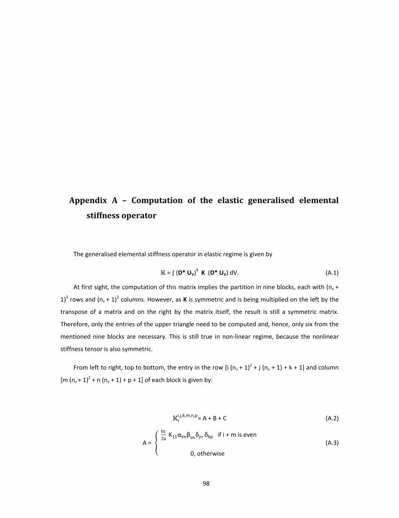
98
Appendix A – Computation of the elastic generalised elemental
stiffness operator
The generalised elemental stiffness operator in elastic regime is given by
= ∫ (D* UV)T K (D* UV) dV. (A.1)
At first sight, the computation of this matrix implies the partition in nine blocks, each with (nv +
1)3 rows and (nv + 1)3 columns. However, as K is symmetric and is being multiplied on the left by the
transpose of a matrix and on the right by the matrix itself, the result is still a symmetric matrix.
Therefore, only the entries of the upper triangle need to be computed and, hence, only six from the
mentioned nine blocks are necessary. This is still true in non-linear regime, because the nonlinear
stiffness tensor is also symmetric.
From left to right, top to bottom, the entry in the row [i (nv + 1)2 + j (nv + 1) + k + 1] and column
[m (nv + 1)2 + n (nv + 1) + p + 1] of each block is given by:
Ii,j,k,m,n,p= A + B + C (A.2)
A = � bc
2a K11αimβimδjn δkp if i + m is even
0, otherwise
@ (A.3)
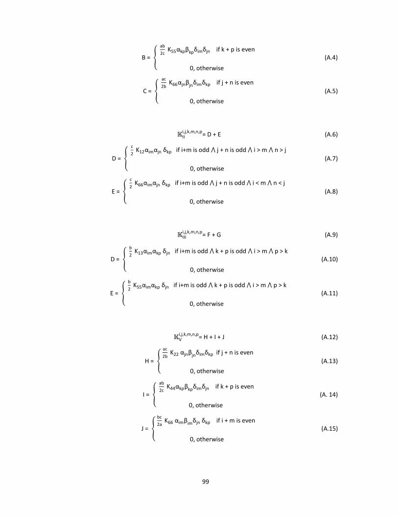
99
B = � ab
2c K55αkpβkpδimδjn if k + p is even
0, otherwise
@ (A.4)
C = � ac
2b K66αjnβjnδimδkp if j + n is even
0, otherwise
@ (A.5)
IIi,j,k,m,n,p= D + E (A.6)
D = � c
2 K12αimαjn δkp if i+m is odd ⋀ j + n is odd ⋀ i > m ⋀ n > j
0, otherwise
@ (A.7)
E = � c
2 K66αimαjn δkp if i+m is odd ⋀ j + n is odd ⋀ i < m ⋀ n < j
0, otherwise
@ (A.8)
IIIi,j,k,m,n,p
= F + G (A.9)
D = � b
2 K13αimαkp δjn if i+m is odd ⋀ k + p is odd ⋀ i > m ⋀ p > k
0, otherwise
@ (A.10)
E = � b
2 K55αimαkp δjn if i+m is odd ⋀ k + p is odd ⋀ i > m ⋀ p > k
0, otherwise
@ (A.11)
Vi,j,k,m,n,p= H + I + J (A.12)
H = � ac
2b K22 αjnβjnδimδkp if j + n is even
0, otherwise
@ (A.13)
I = � ab
2c K44αkpβkpδimδjn if k + p is even
0, otherwise
@ (A. 14)
J = � bc
2a K66 αimβimδjn δkp if i + m is even
0, otherwise
@ (A.15)
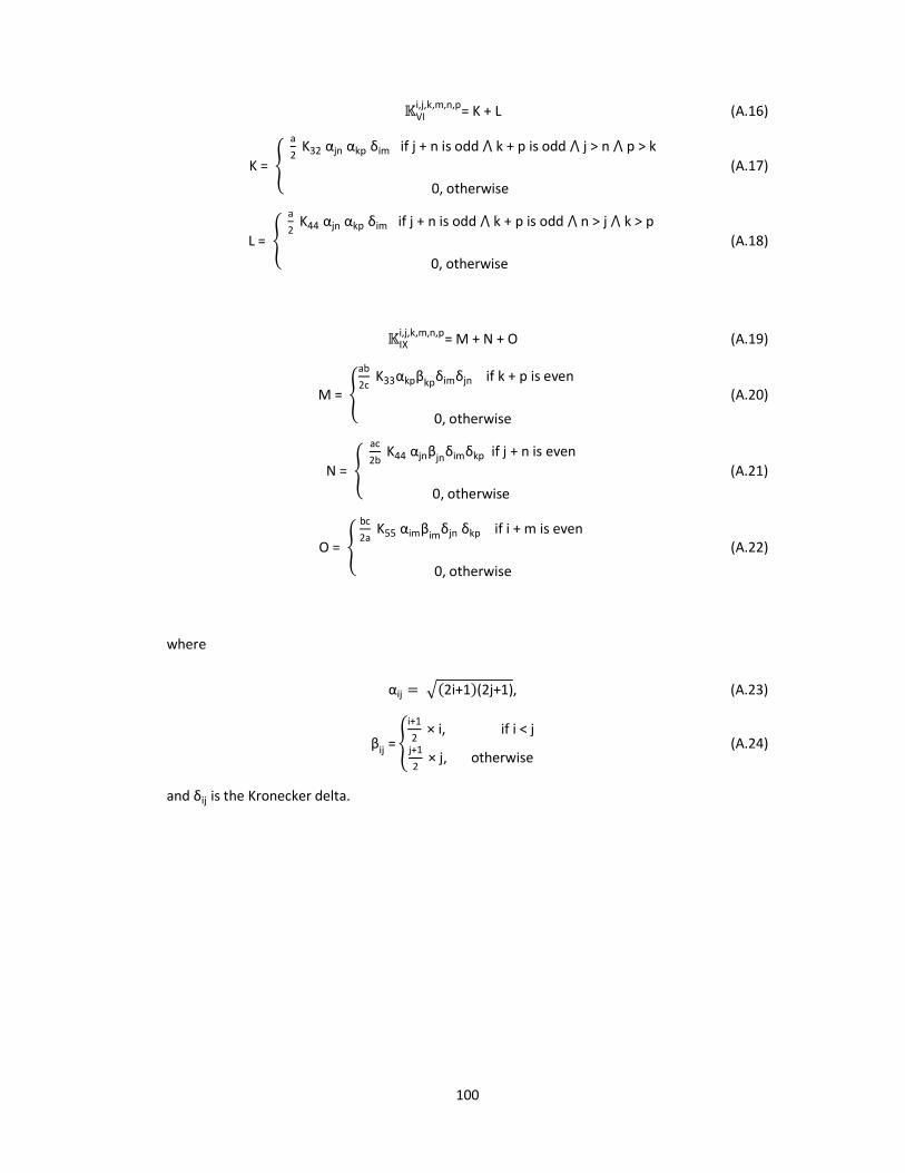
100
VIi,j,k,m,n,p= K + L (A.16)
K = � a
2 K32 αjn αkp δim if j + n is odd ⋀ k + p is odd ⋀ j > n ⋀ p > k
0, otherwise
@ (A.17)
L = � a
2 K44 αjn αkp δim if j + n is odd ⋀ k + p is odd ⋀ n > j ⋀ k > p
0, otherwise
@ (A.18)
IXi,j,k,m,n,p= M + N + O (A.19)
M = �ab
2c K33αkpβkpδimδjn if k + p is even
0, otherwise
@ (A.20)
N = � ac
2b K44 αjnβjnδimδkp if j + n is even
0, otherwise
@ (A.21)
O = � bc
2a K55 αimβimδjn δkp if i + m is even
0, otherwise
@ (A.22)
where
αij � R(2i+1*(2j+1), (A.23)
βij = �i+1
2 × i, if i < j
j+1
2 × j, otherwise
@ (A.24)
and δij is the Kronecker delta.