Modern Topics in Solid-State Theory: Topological ... · Modern Topics in Solid-State Theory: Topological insulators and superconductors Universität Stuttgart. 1. Topological band

Max-Planck-Institut für Festkörperforschung, Stuttgart

Andreas P. Schnyder

January 2016

Modern Topics in Solid-State Theory:Topological insulators and superconductors

Universität Stuttgart

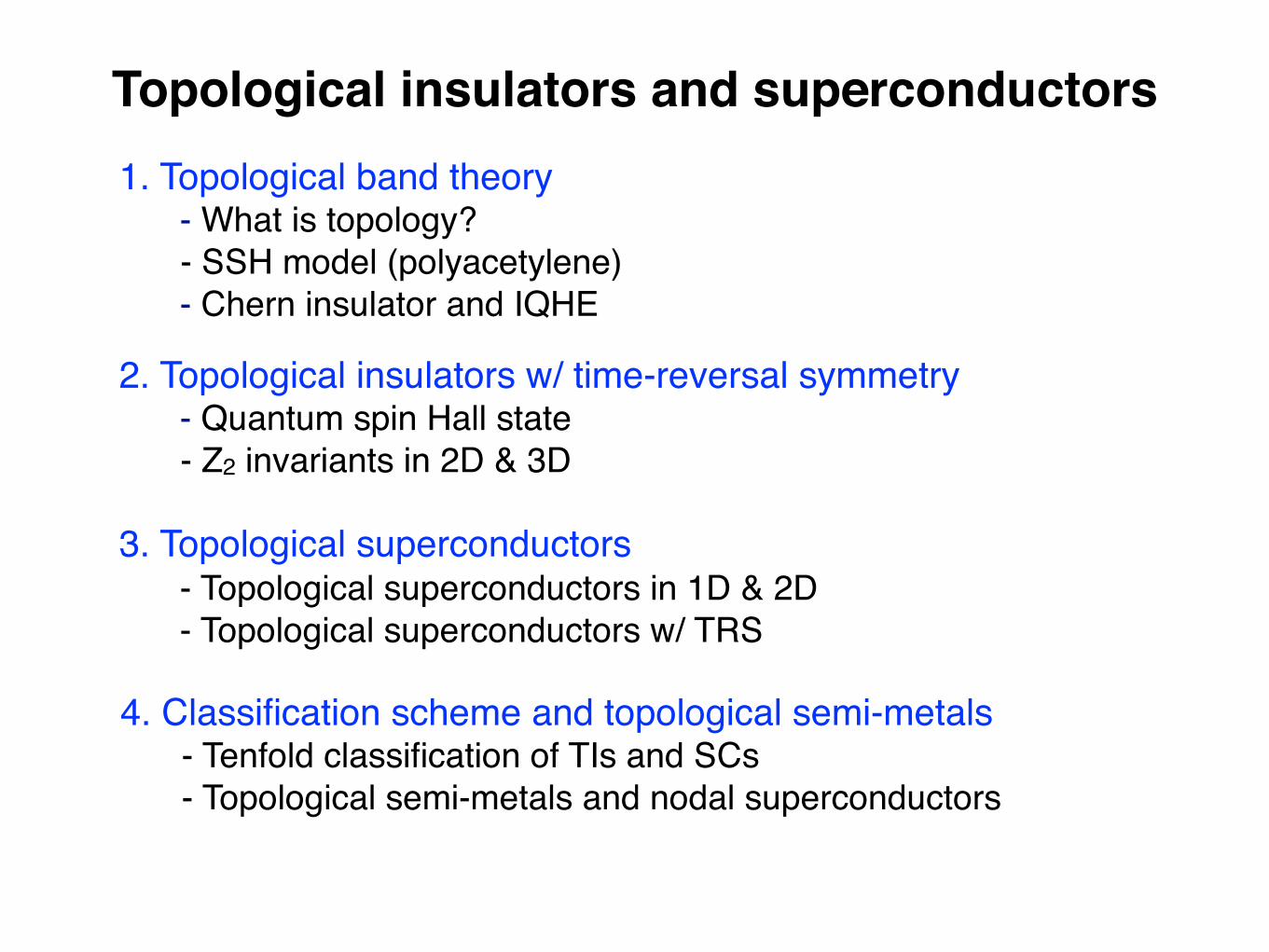
1. Topological band theory- What is topology?

- SSH model (polyacetylene) - Chern insulator and IQHE

3. Topological superconductors - Topological superconductors in 1D & 2D - Topological superconductors w/ TRS

4. Classification scheme and topological semi-metals - Tenfold classification of TIs and SCs - Topological semi-metals and nodal superconductors

Topological insulators and superconductors

2. Topological insulators w/ time-reversal symmetry- Quantum spin Hall state

- Z2 invariants in 2D & 3D

Books and review articles

Review articles:- M.Z. Hasan and C.L. Kane, Rev. Mod. Phys. 82, 3045 (2010)

- X.L. Qi and S.C. Zhang, Rev. Mod. Phys. 83, 1057 (2011) - S. Ryu, A. P. Schnyder, A. Furusaki, A. Ludwig, New J. Phys. 12, 065010 (2010) - C.-K. Chiu, J. C. Y. Teo, A. P. Schnyder, S. Ryu, arXiv:1505.03535 - C. Beenakker, Annual Review of Cond. Mat. Phys. 4, 113 (2013) - J. Alicea, Rep. Prog. Phys. 75, 076501 (2012) - Y. Ando, J. Phys. Soc. Jpn. 82, 102001 (2013) - A. P. Schnyder, P. M. R. Brydon, J. Phys.: CM 27, 243201 (2015) - Y. Ando and L. Fu, arXiv:1501.00531 - E. Witten, arXiv:1510.07698

Books:- Shun-Qing Shen, “Topological insulators”, Springer Series in Solid-State Sciences, Volume 174 (2012)- B. Andrei Bernevig, "Topological Insulators and Topological Superconductors”, Princeton University Press (2013)- Mikio Nakahara, "Geometry, Topology and Physics", Taylor & Francis (2003) - A. Bohm, A. Mostafazadeh, H. Koizumi, Q. Niu, J. Zwanziger, “The geometric phase in quantum systems”, Springer (2003)- M. Franz and L. Molenkamp, “Topological Insulators”, Contemporary Concepts of Condensed Matter Science, Elsevier (2013)

http://arxiv.org/abs/1510.07698

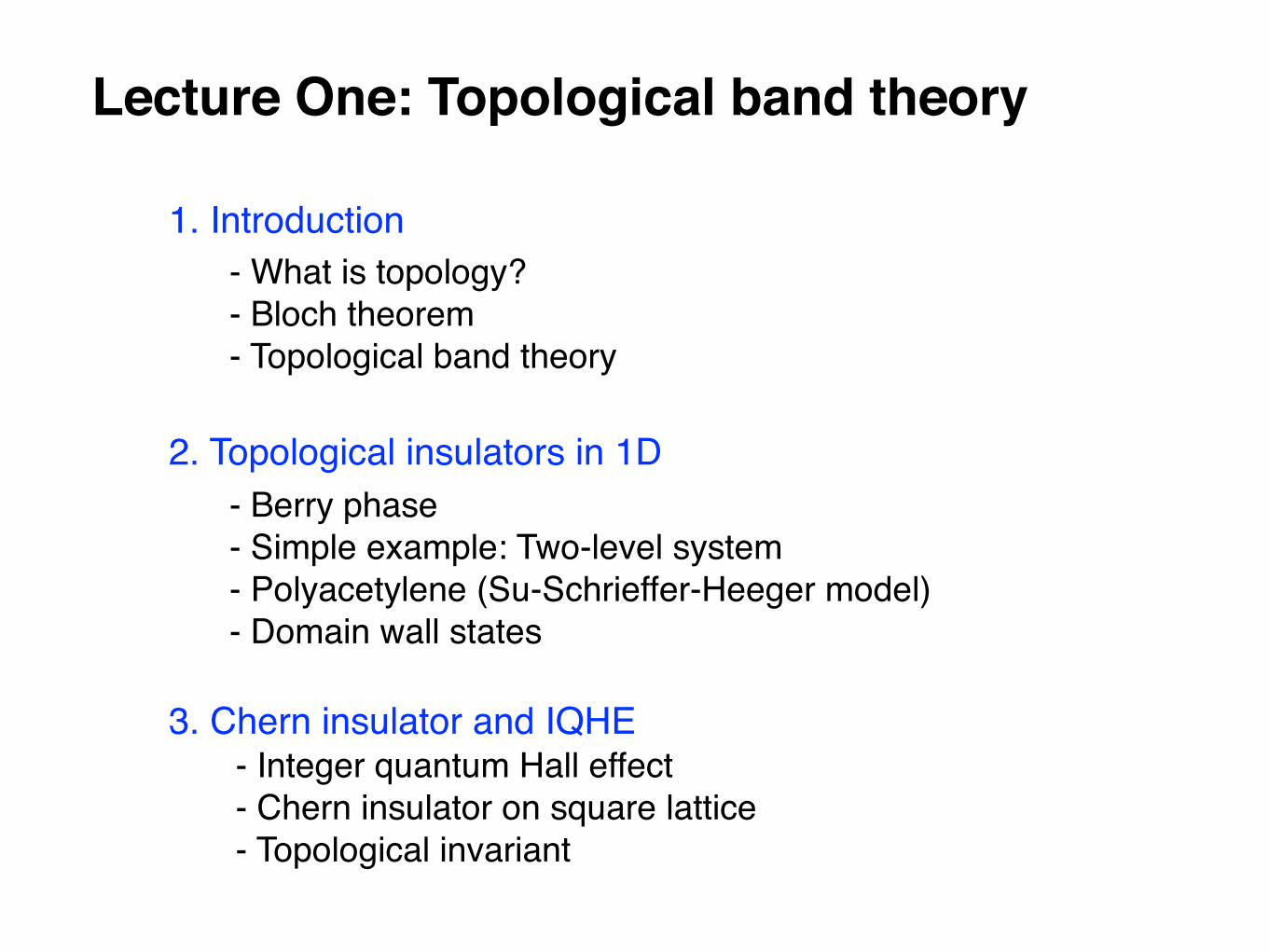
Lecture One: Topological band theory

2. Topological insulators in 1D - Berry phase- Simple example: Two-level system- Polyacetylene (Su-Schrieffer-Heeger model)- Domain wall states

1. Introduction - What is topology?- Bloch theorem- Topological band theory

3. Chern insulator and IQHE- Integer quantum Hall effect- Chern insulator on square lattice- Topological invariant

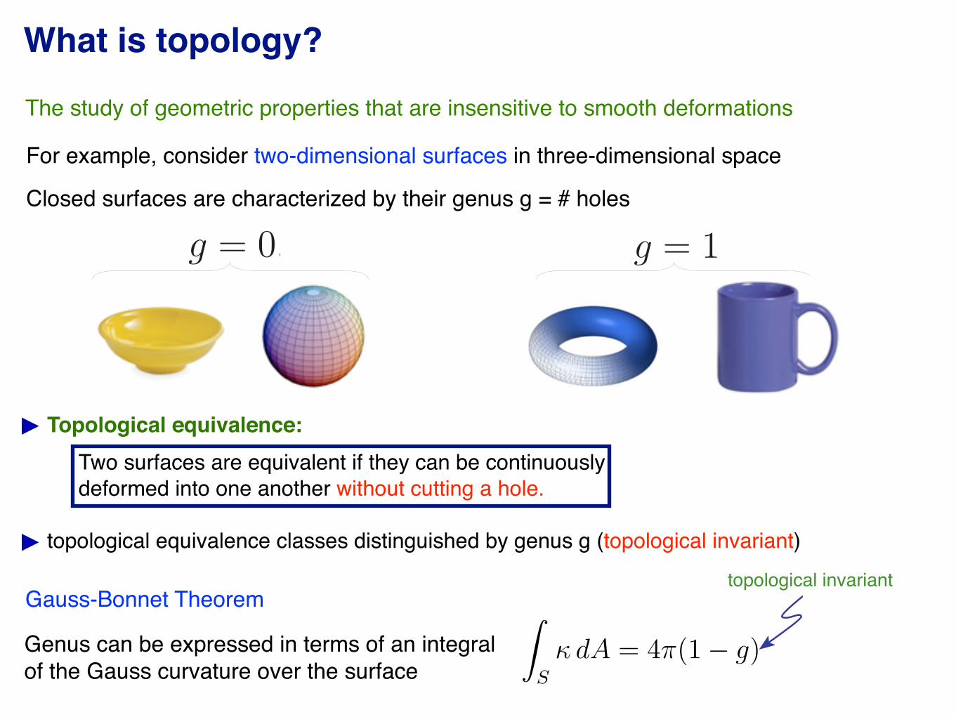
For example, consider two-dimensional surfaces in three-dimensional space

Genus can be expressed in terms of an integral of the Gauss curvature over the surface

What is topology?

The study of geometric properties that are insensitive to smooth deformations

Festkorperphysik II, Musterlosung 11.

Prof. M. Sigrist, WS05/06 ETH Zurich

Gauss:∫

S

κ dA = 4π(1 − g) (1)

Thermal Halll

κxy

T=

π2k2B

6hn (2)

start labels

4s 3p 3s Egap − π/a + π/a (3)

end labels

H(k) (4)

and

W (k∥) = (5)

HBdG =

⎛

⎜

⎜

⎝

εk − gzk

+∆s,k + ∆t,k ε∗⊥k0

+∆s,k + ∆t,k −εk + gzk

0 −ε∗⊥k

ε⊥k0 εk + gz

k−∆s,k + ∆t,k

0 −ε⊥k−∆s,k + ∆t,k −εk − gz

k

⎞

⎟

⎟

⎠

, (6)

and

λL ≫ ξ0 ξ0 = !vF /(π∆0) (7)

(8)

λL > L ≫ ξ0 (9)

charge current operator

jy(x) =iekF /β

2π!

√

λ2 + 1

∑

iωn,ν

+π/2∫

−π/2

dθν sin θν ×

E

Ωνuνvν

(

aheν,ν + aeh

ν,ν

)

e−2iqνx

∣

∣

∣

∣

E→iωn

,

jl,y = +e

!t∑

ky ,σ

sin ky c†lkyσclkyσ −e

!α

∑

ky

cos ky

(

c†lky↓clky↑ + c†lky↑clky↓

)

(9)

(10)

topological invariant

topological equivalence classes distinguished by genus g (topological invariant)

Gauss-Bonnet Theorem

In condensed matter physics:

What is topology?

Closed surfaces are characterized by their genus g = # holesPeriodic Table of Topological Insulators and Superconductors

Anti-Unitary Symmetries :

-Time Reversal :

-Particle -Hole :

Unitary (chiral) symmetry :

1

()

(

)

1

2

;

H

H

k

k

1

()

(

)

1

2

;

H

H

k

k

1

()

()

H

H

k

k ;

Real

K-theory

Complex

K-theory

Bott Periodicity d

Al tland-

Zirnbauer

Random

Matrix

Classes

Kitaev, 2008

Schnyder, Ryu, Furusak i, Ludwig 2008

8 antiunitary symmetry classes



1 frist chapter

Chern number g = 0, g = 1

n =!

bands

i

2π

"

Fdk2 (1)

γC =

#

C

A · dk (2)

First Chern number n = 0

n =!

bands

i

2π

"

dk2

$%

∂u

∂k1

&

&

&

&

∂u

∂k2

'

−%

∂u

∂k2

&

&

&

&

∂u

∂k1

'(

(3)

H(k) :

H(k, k′)

kF > 1/ξ0

sgn(∆+K) = − sgn(∆−

K) and lk antiparallel to lek

sgn(∆+k ) = − sgn(∆−

k )

σxy = ne2

h

ρxy = 1n

he2

n ∈

Jy = σxyEx

Symmetry Operations: Egap = !ωc

ΘH(k)Θ−1 = +H(−k); Θ2 = ±1 (4)

ΞH(k)Ξ−1 = −H(−k); Ξ2 = ±1 (5)

ΠH(k)Π−1 = −H(k); Π ∝ ΘΞ (6)

Θ2 Ξ2 Π2 (7)

Periodic Table of Topological Insulators and Superconductors

Anti-Unitary Symmetries :

-Time Reversal :

-Particle -Hole :

Unitary (chiral) symmetry :

1

()

(

)

1

2

;

H

H

k

k

1

()

(

)

1

2

;

H

H

k

k

1

()

()

H

H

k

k ;

Real

K-theory

Complex

K-theory

Bott Periodicity d

Altland-

Zirnbauer

Random

Matrix

Classes

Kitaev, 2008

Schnyder, Ryu, Furusaki, Ludwig 2008

8 antiunitary symmetry classes



1 frist chapter


n =!

bands

i

2π

"

Fdk2 (1)

γC =

#

C

A · dk (2)


n =!

bands

i

2π

"

dk2

$%

∂u

∂k1

&

&

&

&

∂u

∂k2

'

−%

∂u

∂k2

&

&

&

&

∂u

∂k1

'(

(3)

H(k) :

H(k, k′)

kF > 1/ξ0

sgn(∆+K) = − sgn(∆−


sgn(∆+k ) = − sgn(∆−

k )

σxy = ne2

h

ρxy = 1n

he2

n ∈

Jy = σxyEx


ΘH(k)Θ−1 = +H(−k); Θ2 = ±1 (4)

ΞH(k)Ξ−1 = −H(−k); Ξ2 = ±1 (5)

ΠH(k)Π−1 = −H(k); Π ∝ ΘΞ (6)

Θ2 Ξ2 Π2 (7)

Topological equivalence:Two surfaces are equivalent if they can be continuously deformed into one another without cutting a hole.

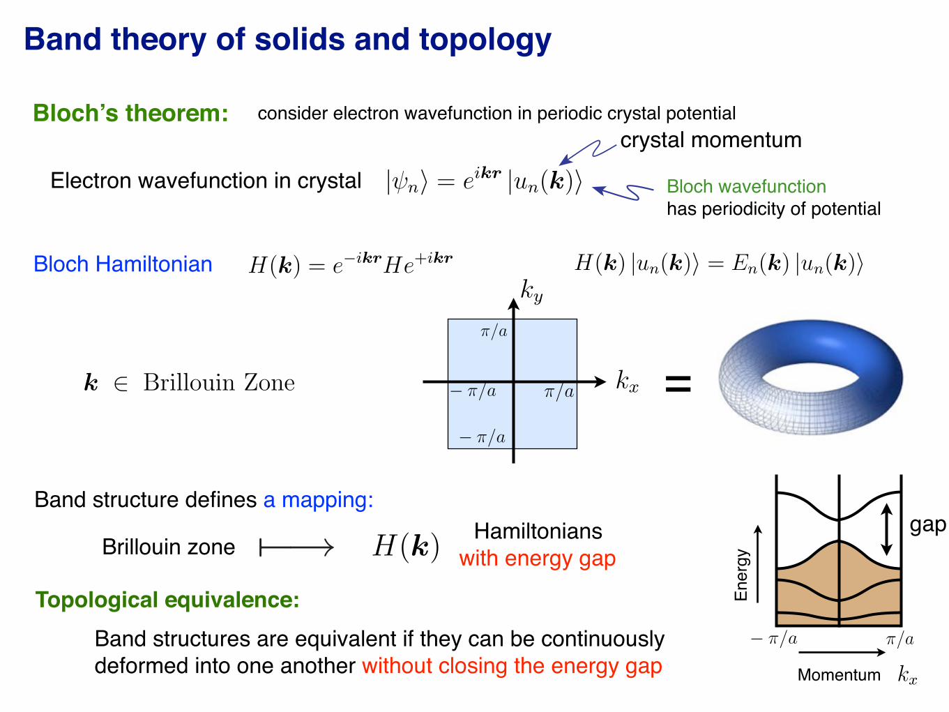
Band theory of solids and topology

Bloch’s theorem:

Topological equivalence:



we have

kx ky π/a − π/a (1)

majoranas

γ1 = ψ + ψ† (2)

γ2 = −i!

ψ − ψ†"

(3)

and

ψ = γ1 + iγ2 (4)

ψ† = γ1 − iγ2 (5)

and

γ2i = 1 (6)

γi, γj = 2δij (7)

mean field

γ†E=0 = γE=0 (8)

⇒ γ†k,E = γ−k,−E (9)

Ξ ψ+k,+E = τxψ∗−k,−E (10)

Ξ2 = +1 Ξ = τxK (11)

τx =

#

0 11 0

$

(12)

c†c c†c ⇒ ⟨c†c†⟩c c = ∆∗c c (13)

weak vs strong

|µ| < 4t (14)

n = 1 (15)

Lattice BdG Hamiltonian

m(k) =m(k)

|m(k)|m(k) : m(k) ∈ S2 π2(S

2) = (16)

HBdG = (2t [cos kx + cos ky] − µ) τz + ∆0 (τx sin kx + τy sin ky) = m(k) · τ (17)

mx my mz (18)



we have


majoranas

γ1 = ψ + ψ† (2)

γ2 = −i!

ψ − ψ†"

(3)

and

ψ = γ1 + iγ2 (4)

ψ† = γ1 − iγ2 (5)

and

γ2i = 1 (6)


mean field

γ†E=0 = γE=0 (8)

⇒ γ†k,E = γ−k,−E (9)

Ξ ψ+k,+E = τxψ∗−k,−E (10)

Ξ2 = +1 Ξ = τxK (11)

τx =

#

0 11 0

$

(12)

c†c c†c ⇒ ⟨c†c†⟩c c = ∆∗c c (13)

weak vs strong

|µ| < 4t (14)

n = 1 (15)


m(k) =m(k)

|m(k)|m(k) : m(k) ∈ S2 π2(S

2) = (16)


mx my mz (18)



we have


majoranas

γ1 = ψ + ψ† (2)

γ2 = −i!

ψ − ψ†"

(3)

and

ψ = γ1 + iγ2 (4)

ψ† = γ1 − iγ2 (5)

and

γ2i = 1 (6)


mean field

γ†E=0 = γE=0 (8)

⇒ γ†k,E = γ−k,−E (9)

Ξ ψ+k,+E = τxψ∗−k,−E (10)

Ξ2 = +1 Ξ = τxK (11)

τx =

#

0 11 0

$

(12)

c†c c†c ⇒ ⟨c†c†⟩c c = ∆∗c c (13)

weak vs strong

|µ| < 4t (14)

n = 1 (15)


m(k) =m(k)

|m(k)|m(k) : m(k) ∈ S2 π2(S

2) = (16)


mx my mz (18)



we have


majoranas

γ1 = ψ + ψ† (2)

γ2 = −i!

ψ − ψ†"

(3)

and

ψ = γ1 + iγ2 (4)

ψ† = γ1 − iγ2 (5)

and

γ2i = 1 (6)


mean field

γ†E=0 = γE=0 (8)

⇒ γ†k,E = γ−k,−E (9)

Ξ ψ+k,+E = τxψ∗−k,−E (10)

Ξ2 = +1 Ξ = τxK (11)

τx =

#

0 11 0

$

(12)

c†c c†c ⇒ ⟨c†c†⟩c c = ∆∗c c (13)

weak vs strong

|µ| < 4t (14)

n = 1 (15)


m(k) =m(k)

|m(k)|m(k) : m(k) ∈ S2 π2(S

2) = (16)


mx my mz (18)



we have


majoranas

γ1 = ψ + ψ† (2)

γ2 = −i!

ψ − ψ†"

(3)

and

ψ = γ1 + iγ2 (4)

ψ† = γ1 − iγ2 (5)

and

γ2i = 1 (6)


mean field

γ†E=0 = γE=0 (8)

⇒ γ†k,E = γ−k,−E (9)

Ξ ψ+k,+E = τxψ∗−k,−E (10)

Ξ2 = +1 Ξ = τxK (11)

τx =

#

0 11 0

$

(12)

c†c c†c ⇒ ⟨c†c†⟩c c = ∆∗c c (13)

weak vs strong

|µ| < 4t (14)

n = 1 (15)


m(k) =m(k)

|m(k)|m(k) : m(k) ∈ S2 π2(S

2) = (16)


mx my mz (18)



we have


majoranas

γ1 = ψ + ψ† (2)

γ2 = −i!

ψ − ψ†"

(3)

and

ψ = γ1 + iγ2 (4)

ψ† = γ1 − iγ2 (5)

and

γ2i = 1 (6)


mean field

γ†E=0 = γE=0 (8)

⇒ γ†k,E = γ−k,−E (9)

Ξ ψ+k,+E = τxψ∗−k,−E (10)

Ξ2 = +1 Ξ = τxK (11)

τx =

#

0 11 0

$

(12)

c†c c†c ⇒ ⟨c†c†⟩c c = ∆∗c c (13)

weak vs strong

|µ| < 4t (14)

n = 1 (15)


m(k) =m(k)

|m(k)|m(k) : m(k) ∈ S2 π2(S

2) = (16)


mx my mz (18)

=

Bloch Hamiltonian



we have

kx ky π/a − π/a k ∈ Brillouin Zone (1)

majoranas

γ1 = ψ + ψ† (2)

γ2 = −i!

ψ − ψ†"

(3)

and

ψ = γ1 + iγ2 (4)

ψ† = γ1 − iγ2 (5)

and

γ2i = 1 (6)


mean field

γ†E=0 = γE=0 (8)

⇒ γ†k,E = γ−k,−E (9)

Ξ ψ+k,+E = τxψ∗−k,−E (10)

Ξ2 = +1 Ξ = τxK (11)

τx =

#

0 11 0

$

(12)

c†c c†c ⇒ ⟨c†c†⟩c c = ∆∗c c (13)

weak vs strong

|µ| < 4t (14)

n = 1 (15)


m(k) =m(k)

|m(k)|m(k) : m(k) ∈ S2 π2(S

2) = (16)


mx my mz (18)

Band structure defines a mapping:Hamiltonians

with energy gapBrillouin zone



1 frist chapter

Ξ HBdG(k) Ξ−1 = −HBdG(−k) "−→ (1)

∆n


n =!

bands

i

2π

"

Fdk2 (2)

γC =

#

C

A · dk (3)


n =!

bands

i

2π

"

dk2

$%

∂u

∂k1

&

&

&

&

∂u

∂k2

'

−%

∂u

∂k2

&

&

&

&

∂u

∂k1

'(

(4)

H(k) :

H(k, k′)

kF > 1/ξ0

sgn(∆+K) = − sgn(∆−


sgn(∆+k ) = − sgn(∆−

k )

σxy = ne2

h

ρxy = 1n

he2

n ∈

Jy = σxyEx


ΘH(k)Θ−1 = +H(−k); Θ2 = ±1 (5)

ΞH(k)Ξ−1 = −H(−k); Ξ2 = ±1 (6)

ΠH(k)Π−1 = −H(k); Π ∝ ΘΞ (7)

Θ2 Ξ2 Π2 (8)



we have

H(k) kx ky π/a − π/a k ∈ Brillouin Zone (1)

majoranas

γ1 = ψ + ψ† (2)

γ2 = −i!

ψ − ψ†"

(3)

and

ψ = γ1 + iγ2 (4)

ψ† = γ1 − iγ2 (5)

and

γ2i = 1 (6)


mean field

γ†E=0 = γE=0 (8)

⇒ γ†k,E = γ−k,−E (9)

Ξ ψ+k,+E = τxψ∗−k,−E (10)

Ξ2 = +1 Ξ = τxK (11)

τx =

#

0 11 0

$

(12)

c†c c†c ⇒ ⟨c†c†⟩c c = ∆∗c c (13)

weak vs strong

|µ| < 4t (14)

n = 1 (15)


m(k) =m(k)

|m(k)|m(k) : m(k) ∈ S2 π2(S

2) = (16)


mx my mz (18)

Band structures are equivalent if they can be continuously deformed into one another without closing the energy gap

Electron wavefunction in crystal

crystal momentum



we have


majoranas

γ1 = ψ + ψ† (2)

γ2 = −i!

ψ − ψ†"

(3)

and

ψ = γ1 + iγ2 (4)

ψ† = γ1 − iγ2 (5)

and

γ2i = 1 (6)


mean field

γ†E=0 = γE=0 (8)

⇒ γ†k,E = γ−k,−E (9)

Ξ ψ+k,+E = τxψ∗−k,−E (10)

Ξ2 = +1 Ξ = τxK (11)

τx =

#

0 11 0

$

(12)

c†c c†c ⇒ ⟨c†c†⟩c c = ∆∗c c (13)

weak vs strong

|µ| < 4t (14)

n = 1 (15)


m(k) =m(k)

|m(k)|m(k) : m(k) ∈ S2 π2(S

2) = (16)


mx my mz (18)



we have


majoranas

γ1 = ψ + ψ† (2)

γ2 = −i!

ψ − ψ†"

(3)

and

ψ = γ1 + iγ2 (4)

ψ† = γ1 − iγ2 (5)

and

γ2i = 1 (6)


mean field

γ†E=0 = γE=0 (8)

⇒ γ†k,E = γ−k,−E (9)

Ξ ψ+k,+E = τxψ∗−k,−E (10)

Ξ2 = +1 Ξ = τxK (11)

τx =

#

0 11 0

$

(12)

c†c c†c ⇒ ⟨c†c†⟩c c = ∆∗c c (13)

weak vs strong

|µ| < 4t (14)

n = 1 (15)


m(k) =m(k)

|m(k)|m(k) : m(k) ∈ S2 π2(S

2) = (16)


mx my mz (18)

Ener

gy

Momentum



homotopy

ν = # kx (1)

∆±k

= ∆s ± ∆t |dk| (2)

∆s > ∆t ∆s ∼ ∆t ν = ±1 for ∆t > ∆s (3)

and

π3[U(2)] = q(k) :∈ U(2) (4)

Lattice BdG HBdG

h(k) = εkσ0 + αgk · σ (5)

∆(k) = (∆sσ0 + ∆tdk · σ) iσy (6)

hex Iy ≃e

!

! kF,−

kF,+

dky

2πsgn

"

#

µ

Hµexρ

µ1 (0, ky)

$

%

− t sin ky + λLx/2#

n=1

ρxn(0, ky) cos ky

&

.(7)

and

jn,ky = −t sin ky

'

c†nky↑cnky↑ + c†nky↓

cnky↓

(

(8)

+ λ cos ky

'

c†nky↓cnky↑ + c†nky↑cnky↓

(

(9)

The contribution j(1)n,ky

corresponds to nearest-neighbor hopping, whereas j(2)n,ky

is due toSOC. We calculate the expectation value of the edge current at zero temperature fromthe spectrum El,ky and the wavefunctions

)

)ψl,ky

*

of H(10)ky

,

Iy = −e

!

1

Ny

#

ky

Lx/2#

n=1

#

l,El<0

⟨ψl,ky |jn,ky|ψl,ky⟩ (10)

We observe that the current operators presence of the superconducting gaps or the edge;these only enter through the eigenstates |ψl,ky⟩.

Momentum dependent topological number:

∝3

#

µ=1

Hµexρ

µ1 (E, ky) ρx

1 (11)

NQPI(ω, q) = −1

πIm

+

#

k

G0(k, ω)T (ω)G0(k + q, ω)

,

∝-

Sf

)

)

)T (ω)

)

)

)Si

.

(12)

a (13)

ξ±k

= εk ± α |gk|(14)



Bloch theorem

[T (R), H ] = 0 |ψn⟩ = eikr |un(k)⟩ (1)

(2)

H(k) = e−ikrHe+ikr (3)

(4)

H(k) |un(k)⟩ = En(k) |un(k)⟩ (5)

we have


majoranas

γ1 = ψ + ψ† (7)

γ2 = −i!

ψ − ψ†"

(8)

and

ψ = γ1 + iγ2 (9)

ψ† = γ1 − iγ2 (10)

and

γ2i = 1 (11)

γi, γj = 2δij (12)

mean field

γ†E=0 = γE=0 (13)

⇒ γ†k,E = γ−k,−E (14)

Ξ ψ+k,+E = τxψ∗−k,−E (15)

Ξ2 = +1 Ξ = τxK (16)

τx =

#

0 11 0

$

(17)

c†c c†c ⇒ ⟨c†c†⟩c c = ∆∗c c (18)

weak vs strong

|µ| < 4t (19)

n = 1 (20)



Bloch theorem

[T (R), H ] = 0 |ψn⟩ = eikr |un(k)⟩ (1)

(2)


(4)

H(k) |un(k)⟩ = En(k) |un(k)⟩ (5)

we have


majoranas

γ1 = ψ + ψ† (7)

γ2 = −i!

ψ − ψ†"

(8)

and

ψ = γ1 + iγ2 (9)

ψ† = γ1 − iγ2 (10)

and

γ2i = 1 (11)

γi, γj = 2δij (12)

mean field

γ†E=0 = γE=0 (13)

⇒ γ†k,E = γ−k,−E (14)

Ξ ψ+k,+E = τxψ∗−k,−E (15)

Ξ2 = +1 Ξ = τxK (16)

τx =

#

0 11 0

$

(17)

c†c c†c ⇒ ⟨c†c†⟩c c = ∆∗c c (18)

weak vs strong

|µ| < 4t (19)

n = 1 (20)



Bloch theorem

[T (R), H ] = 0 |ψn⟩ = eikr |un(k)⟩ (1)

(2)


(4)

H(k) |un(k)⟩ = En(k) |un(k)⟩ (5)

we have


majoranas

γ1 = ψ + ψ† (7)

γ2 = −i!

ψ − ψ†"

(8)

and

ψ = γ1 + iγ2 (9)

ψ† = γ1 − iγ2 (10)

and

γ2i = 1 (11)

γi, γj = 2δij (12)

mean field

γ†E=0 = γE=0 (13)

⇒ γ†k,E = γ−k,−E (14)

Ξ ψ+k,+E = τxψ∗−k,−E (15)

Ξ2 = +1 Ξ = τxK (16)

τx =

#

0 11 0

$

(17)

c†c c†c ⇒ ⟨c†c†⟩c c = ∆∗c c (18)

weak vs strong

|µ| < 4t (19)

n = 1 (20)

Bloch wavefunctionhas periodicity of potential

gap

consider electron wavefunction in periodic crystal potential

Topological band theory BCS Superconductors are similar to insulators

Superconducting gap plays the role of insulating gap

Similar to TI, there are various different topological superconductors with robust surface states

T-breaking superconductor (Moore&Read 2000), T-invariant superconductor ( Schnyder et al

From topological insulators to topological superconductors

Ek

k

Ek

k

Fermi liquid (normal state) Superconducting state

2

normal state



we have


majoranas

γ1 = ψ + ψ† (2)

γ2 = −i!

ψ − ψ†"

(3)

and

ψ = γ1 + iγ2 (4)

ψ† = γ1 − iγ2 (5)

and

γ2i = 1 (6)


mean field

γ†E=0 = γE=0 (8)

⇒ γ†k,E = γ−k,−E (9)

Ξ ψ+k,+E = τxψ∗−k,−E (10)

Ξ2 = +1 Ξ = τxK (11)

τx =

#

0 11 0

$

(12)

c†c c†c ⇒ ⟨c†c†⟩c c = ∆∗c c (13)

weak vs strong

|µ| < 4t (14)

n = 1 (15)


m(k) =m(k)

|m(k)|m(k) : m(k) ∈ S2 π2(S

2) = (16)


mx my mz (18)



we have


majoranas

γ1 = ψ + ψ† (2)

γ2 = −i!

ψ − ψ†"

(3)

and

ψ = γ1 + iγ2 (4)

ψ† = γ1 − iγ2 (5)

and

γ2i = 1 (6)


mean field

γ†E=0 = γE=0 (8)

⇒ γ†k,E = γ−k,−E (9)

Ξ ψ+k,+E = τxψ∗−k,−E (10)

Ξ2 = +1 Ξ = τxK (11)

τx =

#

0 11 0

$

(12)

c†c c†c ⇒ ⟨c†c†⟩c c = ∆∗c c (13)

weak vs strong

|µ| < 4t (14)

n = 1 (15)


m(k) =m(k)

|m(k)|m(k) : m(k) ∈ S2 π2(S

2) = (16)


mx my mz (18)

Ener

gy

crystal momentum



homotopy

ν = # kx (1)

∆±k

= ∆s ± ∆t |dk| (2)

∆s > ∆t ∆s ∼ ∆t ν = ±1 for ∆t > ∆s (3)

and

π3[U(2)] = q(k) :∈ U(2) (4)

Lattice BdG HBdG

h(k) = εkσ0 + αgk · σ (5)

∆(k) = (∆sσ0 + ∆tdk · σ) iσy (6)

hex Iy ≃e

!

! kF,−

kF,+

dky

2πsgn

"

#

µ

Hµexρ

µ1 (0, ky)

$

%


n=1

ρxn(0, ky) cos ky

&

.(7)

and

jn,ky = −t sin ky

'


cnky↓

(

(8)

+ λ cos ky

'


(

(9)




)

)ψl,ky

*

of H(10)ky

,

Iy = −e

!

1

Ny

#

ky

Lx/2#

n=1

#

l,El<0




∝3

#

µ=1

Hµexρ

µ1 (E, ky) ρx

1 (11)

NQPI(ω, q) = −1

πIm

+

#

k

G0(k, ω)T (ω)G0(k + q, ω)

,

∝-

Sf

)

)

)T (ω)

)

)

)Si

.

(12)

a (13)

ξ±k

= εk ± α |gk|(14)

gap

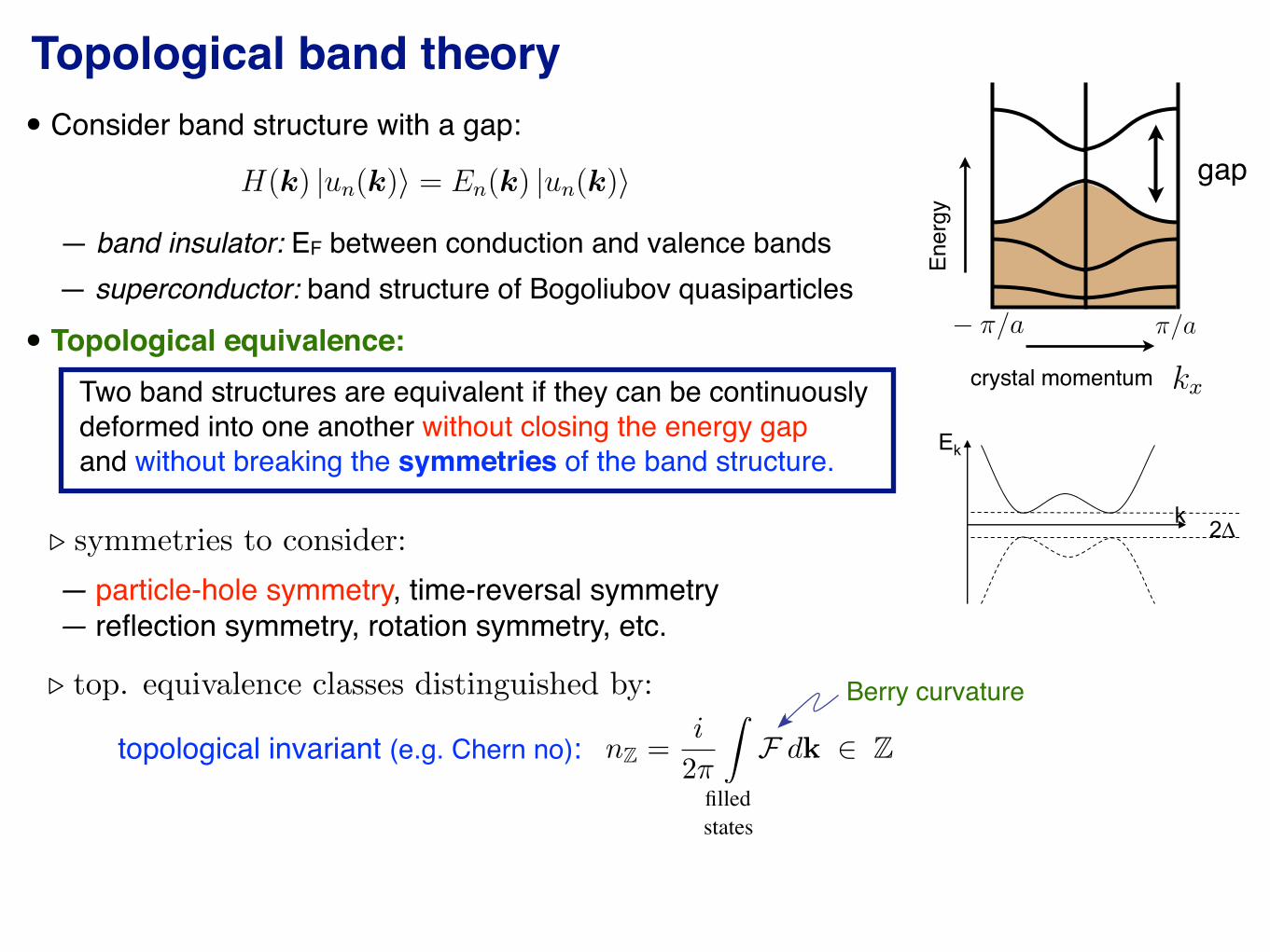
— band insulator: EF between conduction and valence bands



Bloch theorem

[T (R), H ] = 0 |ψn⟩ = eikr |un(k)⟩ (1)

(2)


(4)

H(k) |un(k)⟩ = En(k) |un(k)⟩ (5)

we have


majoranas

γ1 = ψ + ψ† (7)

γ2 = −i!

ψ − ψ†"

(8)

and

ψ = γ1 + iγ2 (9)

ψ† = γ1 − iγ2 (10)

and

γ2i = 1 (11)

γi, γj = 2δij (12)

mean field

γ†E=0 = γE=0 (13)

⇒ γ†k,E = γ−k,−E (14)

Ξ ψ+k,+E = τxψ∗−k,−E (15)

Ξ2 = +1 Ξ = τxK (16)

τx =

#

0 11 0

$

(17)

c†c c†c ⇒ ⟨c†c†⟩c c = ∆∗c c (18)

weak vs strong

|µ| < 4t (19)

n = 1 (20)

— superconductor: band structure of Bogoliubov quasiparticles

• Topological equivalence:

• Consider band structure with a gap:

. symmetries to consider:

. top. equivalence classes distinguished by:

— particle-hole symmetry, time-reversal symmetry — reflection symmetry, rotation symmetry, etc.

topological invariant (e.g. Chern no):

Berry curvature

nZ =i

2

ZF dk 2 Z

filledstates

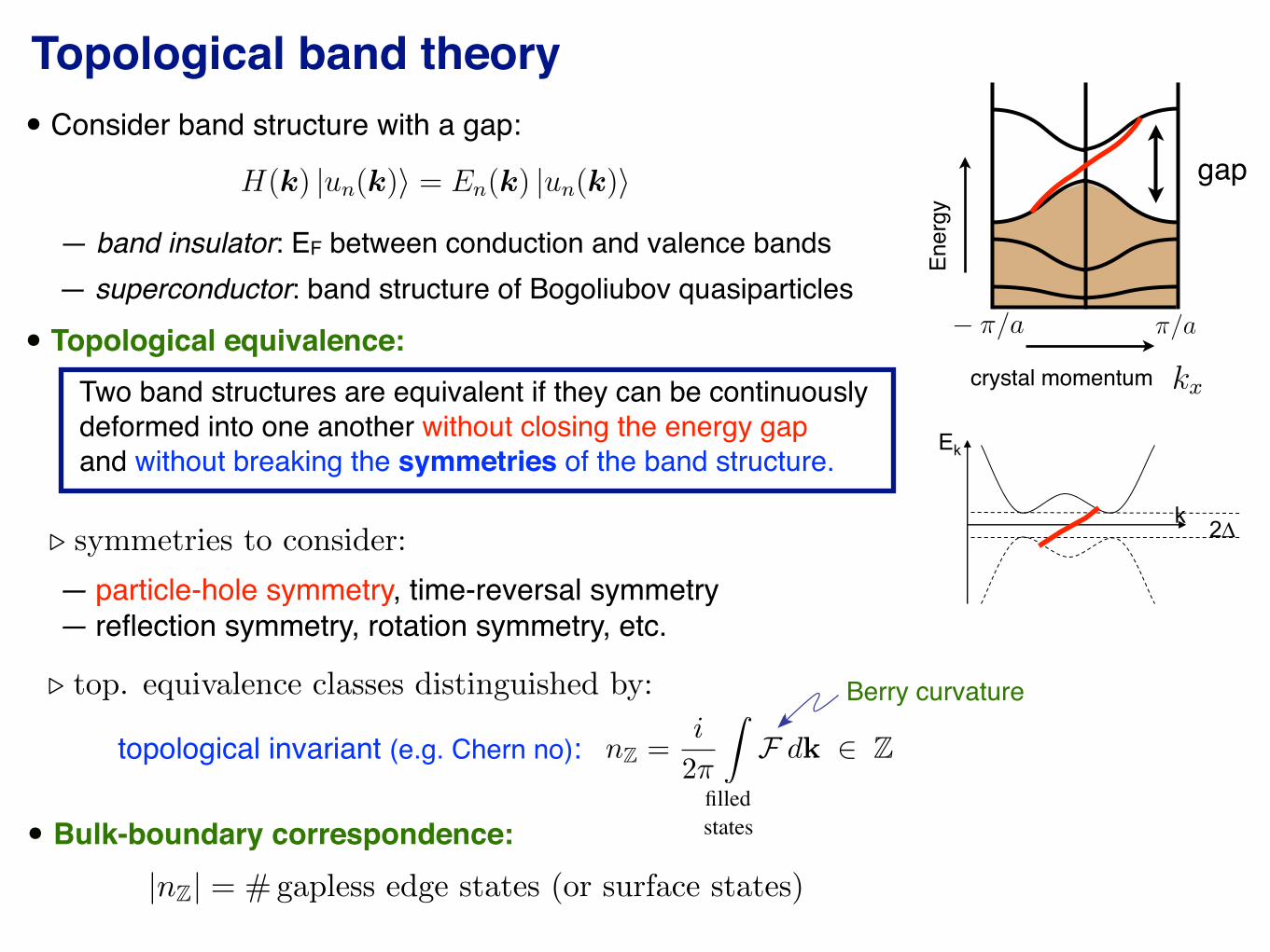
Two band structures are equivalent if they can be continuously deformed into one another without closing the energy gap and without breaking the symmetries of the band structure.

Topological band theory BCS Superconductors are similar to insulators

Superconducting gap plays the role of insulating gap

Similar to TI, there are various different topological superconductors with robust surface states

T-breaking superconductor (Moore&Read 2000), T-invariant superconductor ( Schnyder et al

From topological insulators to topological superconductors

Ek

k

Ek

k

Fermi liquid (normal state) Superconducting state

2

normal stateTwo band structures are equivalent if they can be continuously deformed into one another without closing the energy gap and without breaking the symmetries of the band structure.

topological invariant (e.g. Chern no):

— particle-hole symmetry, time-reversal symmetry — reflection symmetry, rotation symmetry, etc.



we have


majoranas

γ1 = ψ + ψ† (2)

γ2 = −i!

ψ − ψ†"

(3)

and

ψ = γ1 + iγ2 (4)

ψ† = γ1 − iγ2 (5)

and

γ2i = 1 (6)


mean field

γ†E=0 = γE=0 (8)

⇒ γ†k,E = γ−k,−E (9)

Ξ ψ+k,+E = τxψ∗−k,−E (10)

Ξ2 = +1 Ξ = τxK (11)

τx =

#

0 11 0

$

(12)

c†c c†c ⇒ ⟨c†c†⟩c c = ∆∗c c (13)

weak vs strong

|µ| < 4t (14)

n = 1 (15)


m(k) =m(k)

|m(k)|m(k) : m(k) ∈ S2 π2(S

2) = (16)


mx my mz (18)



we have


majoranas

γ1 = ψ + ψ† (2)

γ2 = −i!

ψ − ψ†"

(3)

and

ψ = γ1 + iγ2 (4)

ψ† = γ1 − iγ2 (5)

and

γ2i = 1 (6)


mean field

γ†E=0 = γE=0 (8)

⇒ γ†k,E = γ−k,−E (9)

Ξ ψ+k,+E = τxψ∗−k,−E (10)

Ξ2 = +1 Ξ = τxK (11)

τx =

#

0 11 0

$

(12)

c†c c†c ⇒ ⟨c†c†⟩c c = ∆∗c c (13)

weak vs strong

|µ| < 4t (14)

n = 1 (15)


m(k) =m(k)

|m(k)|m(k) : m(k) ∈ S2 π2(S

2) = (16)


mx my mz (18)

Ener

gy



homotopy

ν = # kx (1)

∆±k

= ∆s ± ∆t |dk| (2)

∆s > ∆t ∆s ∼ ∆t ν = ±1 for ∆t > ∆s (3)

and

π3[U(2)] = q(k) :∈ U(2) (4)

Lattice BdG HBdG

h(k) = εkσ0 + αgk · σ (5)

∆(k) = (∆sσ0 + ∆tdk · σ) iσy (6)

hex Iy ≃e

!

! kF,−

kF,+

dky

2πsgn

"

#

µ

Hµexρ

µ1 (0, ky)

$

%


n=1

ρxn(0, ky) cos ky

&

.(7)

and

jn,ky = −t sin ky

'


cnky↓

(

(8)

+ λ cos ky

'


(

(9)




)

)ψl,ky

*

of H(10)ky

,

Iy = −e

!

1

Ny

#

ky

Lx/2#

n=1

#

l,El<0




∝3

#

µ=1

Hµexρ

µ1 (E, ky) ρx

1 (11)

NQPI(ω, q) = −1

πIm

+

#

k

G0(k, ω)T (ω)G0(k + q, ω)

,

∝-

Sf

)

)

)T (ω)

)

)

)Si

.

(12)

a (13)

ξ±k

= εk ± α |gk|(14)

gap

— band insulator: EF between conduction and valence bands



Bloch theorem

[T (R), H ] = 0 |ψn⟩ = eikr |un(k)⟩ (1)

(2)


(4)

H(k) |un(k)⟩ = En(k) |un(k)⟩ (5)

we have


majoranas

γ1 = ψ + ψ† (7)

γ2 = −i!

ψ − ψ†"

(8)

and

ψ = γ1 + iγ2 (9)

ψ† = γ1 − iγ2 (10)

and

γ2i = 1 (11)

γi, γj = 2δij (12)

mean field

γ†E=0 = γE=0 (13)

⇒ γ†k,E = γ−k,−E (14)

Ξ ψ+k,+E = τxψ∗−k,−E (15)

Ξ2 = +1 Ξ = τxK (16)

τx =

#

0 11 0

$

(17)

c†c c†c ⇒ ⟨c†c†⟩c c = ∆∗c c (18)

weak vs strong

|µ| < 4t (19)

n = 1 (20)

— superconductor: band structure of Bogoliubov quasiparticles

• Topological equivalence:

• Consider band structure with a gap:

Berry curvature

• Bulk-boundary correspondence:

. symmetries to consider:

. top. equivalence classes distinguished by:

|nZ| = #gapless edge states (or surface states)

nZ =i

2

ZF dk 2 Z

filledstates

crystal momentum

Topological invariants of band structures:

I. NON-CENTROSYMMETRIC SUPERCONDUCTORS: GENERAL FORMALISM

Gauss Bonnet∫

M

κ dA = 2πχ = 2π(2 − 2g) (1.1)

Berry connection

A = ⟨uk|− i∇k |uk⟩ (1.2)

F = ∇× A (1.3)

We consider a model Hamiltonian for a BCS superconductor in a non-centrosymmetric crystal.

In particular we have Li2PdxPt3−xB in mind. In the following sx, sy, sz denote the Pauli matrices

in the spin grading, whereas τx, τy, τz denote the Pauli matrices in the particle-hole grading. We

start from a general time-reversal invariant superconductor with the Hamiltonian

H =∑

k

(

ψ†k

ψT−k

)

H(k)

⎛

⎝

ψk

ψ†T−k

⎞

⎠ , H(k) =

⎛

⎝

h(k) ∆(k)

∆†(k) −hT (−k)

⎞

⎠ . (1.4)

We start from the Hamiltonian

H =1

2

∑

k

(

c†k↑ c†

k↓ c−k↑ c−k↓

)

Hk

⎛

⎜

⎜

⎜

⎜

⎜

⎝

ck↑

ck↓

c†−k↑

c†−k↓

⎞

⎟

⎟

⎟

⎟

⎟

⎠

, Hk =

⎛

⎝

Ξk ∆k

∆†k−ΞT

−k

⎞

⎠ , (1.5a)

with the matrix elements

Ξk = εks0 + gk · s, ∆k = (ψk + dk · s) (isy) , (1.5b)

the bare band dispersion is for simplicity assumed to be

εk = t1 (cos kx + cos ky + cos kz) − µ (1.5c)

(which is assumed to be time-reversal invariant εk = ε−k). Here we shall use the following

parameters (t1, µ) = (1.0, 1.8). The spin-orbit coupling is parameterized by

gk = αlk = α (lxkx + lyky + lzkz) = α(x sin ky − y sin kx), (1.5d)

where g−k = −gk. For lzk

= 0, this is called Rashba-type spin-orbit coupling. The spin-orbit

coupling strength is taken to be α = 0.05. This asymmetric spin-orbit coupling leads to a mixing

3

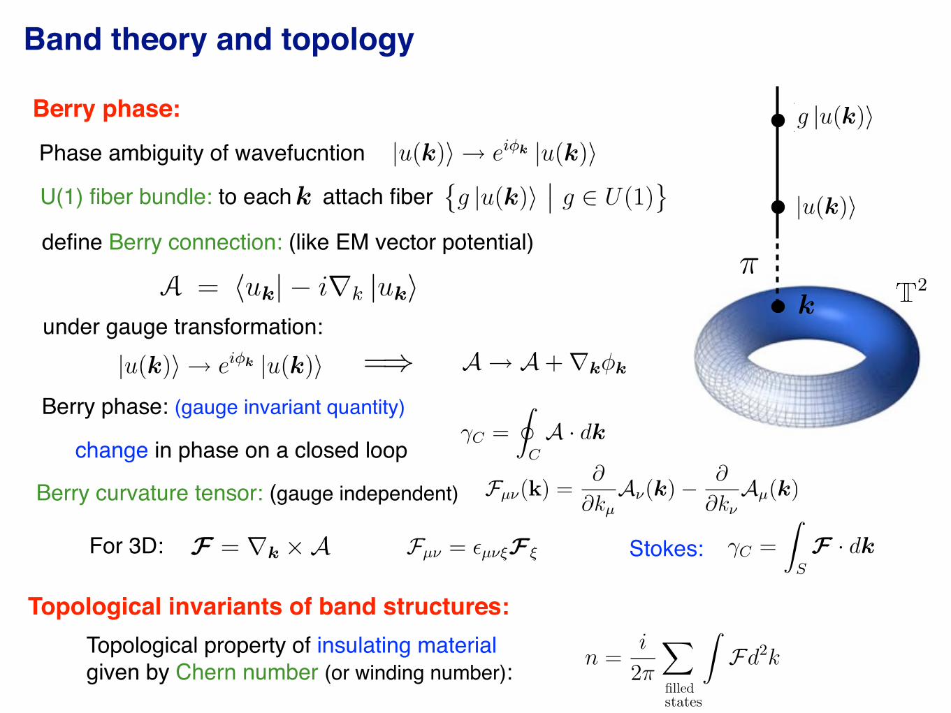
define Berry connection: (like EM vector potential)

Berry curvature tensor: (gauge independent)

Topological property of insulating material given by Chern number (or winding number):

Band theory and topology

Berry phase:

Phase ambiguity of wavefucntion



and

|u(k)⟩ → eiφk |u(k)⟩ (1)

Bloch theorem

[T (R), H ] = 0 k |ψn⟩ = eikr |un(k)⟩ (2)

(3)


(5)

H(k) |un(k)⟩ = En(k) |un(k)⟩ (6)

we have


majoranas

γ1 = ψ + ψ† (8)

γ2 = −i!

ψ − ψ†"

(9)

and

ψ = γ1 + iγ2 (10)

ψ† = γ1 − iγ2 (11)

and

γ2i = 1 (12)

γi, γj = 2δij (13)

mean field

γ†E=0 = γE=0 (14)

⇒ γ†k,E = γ−k,−E (15)

Ξ ψ+k,+E = τxψ∗−k,−E (16)

Ξ2 = +1 Ξ = τxK (17)

τx =

#

0 11 0

$

(18)

c†c c†c ⇒ ⟨c†c†⟩c c = ∆∗c c (19)

weak vs strong

|µ| < 4t (20)

n = 1 (21)



and

|u(k)⟩ → eiφk |u(k)⟩ (1)

A → A + ∇kφk (2)

Bloch theorem

[T (R), H ] = 0 k |ψn⟩ = eikr |un(k)⟩ (3)

(4)


(6)

H(k) |un(k)⟩ = En(k) |un(k)⟩ (7)

we have


majoranas

γ1 = ψ + ψ† (9)

γ2 = −i!

ψ − ψ†"

(10)

and

ψ = γ1 + iγ2 (11)

ψ† = γ1 − iγ2 (12)

and

γ2i = 1 (13)

γi, γj = 2δij (14)

mean field

γ†E=0 = γE=0 (15)

⇒ γ†k,E = γ−k,−E (16)

Ξ ψ+k,+E = τxψ∗−k,−E (17)

Ξ2 = +1 Ξ = τxK (18)

τx =

#

0 11 0

$

(19)

c†c c†c ⇒ ⟨c†c†⟩c c = ∆∗c c (20)



and

|u(k)⟩ → eiφk |u(k)⟩ (1)

A → A + ∇kφk (2)

F = ∇k ×A (3)

γC =

!

C

A · dk (4)

Bloch theorem

[T (R), H ] = 0 k |ψn⟩ = eikr |un(k)⟩ (5)

(6)


(8)

H(k) |un(k)⟩ = En(k) |un(k)⟩ (9)

we have


majoranas

γ1 = ψ + ψ† (11)

γ2 = −i"

ψ − ψ†#

(12)

and

ψ = γ1 + iγ2 (13)

ψ† = γ1 − iγ2 (14)

and

γ2i = 1 (15)

γi, γj = 2δij (16)

mean field

γ†E=0 = γE=0 (17)

⇒ γ†k,E = γ−k,−E (18)

Ξ ψ+k,+E = τxψ∗−k,−E (19)

Ξ2 = +1 Ξ = τxK (20)

τx =

$

0 11 0

%

(21)

c†c c†c ⇒ ⟨c†c†⟩c c = ∆∗c c (22)

under gauge transformation:



and

|u(k)⟩ → eiφk |u(k)⟩ (1)

Bloch theorem

[T (R), H ] = 0 k |ψn⟩ = eikr |un(k)⟩ (2)

(3)


(5)

H(k) |un(k)⟩ = En(k) |un(k)⟩ (6)

we have


majoranas

γ1 = ψ + ψ† (8)

γ2 = −i!

ψ − ψ†"

(9)

and

ψ = γ1 + iγ2 (10)

ψ† = γ1 − iγ2 (11)

and

γ2i = 1 (12)

γi, γj = 2δij (13)

mean field

γ†E=0 = γE=0 (14)

⇒ γ†k,E = γ−k,−E (15)

Ξ ψ+k,+E = τxψ∗−k,−E (16)

Ξ2 = +1 Ξ = τxK (17)

τx =

#

0 11 0

$

(18)

c†c c†c ⇒ ⟨c†c†⟩c c = ∆∗c c (19)

weak vs strong

|µ| < 4t (20)

n = 1 (21)



and

|u(k)⟩ → eiφk |u(k)⟩ (1)

A → A + ∇kφk (2)

F = ∇k ×A (3)

γC =

!

C

A · dk (4)

γC =

"

S

Fd2k (5)

=⇒ (6)

Bloch theorem

[T (R), H ] = 0 k |ψn⟩ = eikr |un(k)⟩ (7)

(8)


(10)

H(k) |un(k)⟩ = En(k) |un(k)⟩ (11)

we have


majoranas

γ1 = ψ + ψ† (13)

γ2 = −i#

ψ − ψ†$

(14)

and

ψ = γ1 + iγ2 (15)

ψ† = γ1 − iγ2 (16)

and

γ2i = 1 (17)

γi, γj = 2δij (18)

Berry phase: (gauge invariant quantity)



Chern number

n =i

2π

∫

F dk filled states (1)

Gauss:∫

S

κ dA = 4π(1 − g) (2)

Thermal Halll

κxy

T=

π2k2B

6hn (3)

start labels

4s 3p 3s Egap − π/a + π/a (4)

end labels

H(k) (5)

and

W (k∥) = (6)

HBdG =

⎛

⎜

⎜

⎝

εk − gzk

+∆s,k + ∆t,k ε∗⊥k0


0 −ε∗⊥k

ε⊥k0 εk + gz

k−∆s,k + ∆t,k

0 −ε⊥k−∆s,k + ∆t,k −εk − gz

k

⎞

⎟

⎟

⎠

, (7)

and

λL ≫ ξ0 ξ0 = !vF /(π∆0) (8)

(9)

λL > L ≫ ξ0 (10)


jy(x) =iekF /β

2π!

√

λ2 + 1

∑

iωn,ν

+π/2∫

−π/2

dθν sin θν ×

E

Ωνuνvν

(

aheν,ν + aeh

ν,ν

)

e−2iqνx

∣

∣

∣

∣

E→iωn

,

jl,y = +e

!t∑

ky ,σ


!α

∑

ky

cos ky

(


)

(10)

(11)



Chern number

n =i

2π

∫

F dk filled states (1)

Gauss:∫

S

κ dA = 4π(1 − g) (2)

Thermal Halll

κxy

T=

π2k2B

6hn (3)

start labels

4s 3p 3s Egap − π/a + π/a (4)

end labels

H(k) (5)

and

W (k∥) = (6)

HBdG =

⎛

⎜

⎜

⎝

εk − gzk

+∆s,k + ∆t,k ε∗⊥k0


0 −ε∗⊥k

ε⊥k0 εk + gz

k−∆s,k + ∆t,k

0 −ε⊥k−∆s,k + ∆t,k −εk − gz

k

⎞

⎟

⎟

⎠

, (7)

and

λL ≫ ξ0 ξ0 = !vF /(π∆0) (8)

(9)

λL > L ≫ ξ0 (10)


jy(x) =iekF /β

2π!

√

λ2 + 1

∑

iωn,ν

+π/2∫

−π/2

dθν sin θν ×

E

Ωνuνvν

(

aheν,ν + aeh

ν,ν

)

e−2iqνx

∣

∣

∣

∣

E→iωn

,

jl,y = +e

!t∑

ky ,σ


!α

∑

ky

cos ky

(


)

(10)

(11)



and

n =i

2π

!

"

Fd2k (1)

|u(k)⟩ → eiφk |u(k)⟩ (2)

A → A + ∇kφk (3)

F = ∇k ×A (4)

γC =

#

C

A · dk (5)

γC =

"

S

Fd2k (6)

=⇒ (7)

Bloch theorem

[T (R), H ] = 0 k |ψn⟩ = eikr |un(k)⟩ (8)

(9)


(11)

H(k) |un(k)⟩ = En(k) |un(k)⟩ (12)

we have


majoranas

γ1 = ψ + ψ† (14)

γ2 = −i$

ψ − ψ†%

(15)

and

ψ = γ1 + iγ2 (16)

ψ† = γ1 − iγ2 (17)

and

γ2i = 1 (18)

γi, γj = 2δij (19)

change in phase on a closed loop

U(1) fiber bundle: to each attach fiber

Festk

¨

orperphysik II, Musterl

¨

osung 11.


and this

k (1)

22s (E = 0.6)

ijs 1/

|q| 2E/t (2)

and this

gk = kzz

+(kx + ky)(x + y) (3)

some more

kx kz (4)

k q = 2k A(E,k) 00s ij

s i, j 1, 2, 3 (5)

s (E,q) = 1

d2k

(2)2Tr

SG(0)(E,k + q)V G0(E,k)

11

(6)

qx qy (7)

0s i

s , i 1, 2, 3 = 0 1, 2, 3 (8)

and this is it:

s (E,q) = 1

2i

(E,q)

(E,q)

, (9)

and

Gnn(E,k,q) =

nn

G(0)nn(E,k

)VnnG

(0)nn(E,k), (10)

and

(E,q) =

d2k

(2)2Tr

SG(0)(E,k + q)V G0(E,k)

11

. (11)

More formulas I need:

q = kf ki kf ki = 2/|q| (12)

these are the formulas I need:

00s ij

s |q| = 2E/t

1/qx qx = ±2E/t (13)

Festk

¨


¨

osung 11.


and this

kg |u(k)

g U(1)

(1)

22s (E = 0.6)

ijs 1/

|q| 2E/t (2)

and this

gk = kzz

+(kx + ky)(x + y) (3)

some more

kx kz (4)


s i, j 1, 2, 3 (5)

s (E,q) = 1

d2k

(2)2Tr

SG(0)(E,k + q)V G0(E,k)

11

(6)

qx qy (7)

0s i

s , i 1, 2, 3 = 0 1, 2, 3 (8)

and this is it:

s (E,q) = 1

2i

(E,q)

(E,q)

, (9)

and

Gnn(E,k,q) =

nn

G(0)nn(E,k

)VnnG

(0)nn(E,k), (10)

and

(E,q) =

d2k

(2)2Tr

SG(0)(E,k + q)V G0(E,k)

11

. (11)


q = kf ki kf ki = 2/|q| (12)


00s ij

s |q| = 2E/t

1/qx qx = ±2E/t (13)

Festk

¨


¨

osung 11.


and this

kg |u(k)

g U(1)

(1)

22s (E = 0.6)

ijs 1/

|q| 2E/t (2)

and this

gk = kzz

+(kx + ky)(x + y) (3)

some more

kx kz (4)


s i, j 1, 2, 3 (5)

s (E,q) = 1

d2k

(2)2Tr

SG(0)(E,k + q)V G0(E,k)

11

(6)

qx qy (7)

0s i

s , i 1, 2, 3 = 0 1, 2, 3 (8)

and this is it:

s (E,q) = 1

2i

(E,q)

(E,q)

, (9)

and

Gnn(E,k,q) =

nn

G(0)nn(E,k

)VnnG

(0)nn(E,k), (10)

and

(E,q) =

d2k

(2)2Tr

SG(0)(E,k + q)V G0(E,k)

11

. (11)


q = kf ki kf ki = 2/|q| (12)


00s ij

s |q| = 2E/t

1/qx qx = ±2E/t (13)

Festk

¨


¨

osung 11.


and this

kg |u(k)

g U(1)

(1)

22s (E = 0.6)

ijs 1/

|q| 2E/t (2)

and this

gk = kzz

+(kx + ky)(x + y) (3)

some more

kx kz (4)


s i, j 1, 2, 3 (5)

s (E,q) = 1

d2k

(2)2Tr

SG(0)(E,k + q)V G0(E,k)

11

(6)

qx qy (7)

0s i

s , i 1, 2, 3 = 0 1, 2, 3 (8)

and this is it:

s (E,q) = 1

2i

(E,q)

(E,q)

, (9)

and

Gnn(E,k,q) =

nn

G(0)nn(E,k

)VnnG

(0)nn(E,k), (10)

and

(E,q) =

d2k

(2)2Tr

SG(0)(E,k + q)V G0(E,k)

11

. (11)


q = kf ki kf ki = 2/|q| (12)


00s ij

s |q| = 2E/t

1/qx qx = ±2E/t (13)

Festk

¨


¨

osung 11.


and this

k (1)

22s (E = 0.6)

ijs 1/

|q| 2E/t (2)

and this

gk = kzz

+(kx + ky)(x + y) (3)

some more

kx kz (4)


s i, j 1, 2, 3 (5)

s (E,q) = 1

d2k

(2)2Tr

SG(0)(E,k + q)V G0(E,k)

11

(6)

qx qy (7)

0s i

s , i 1, 2, 3 = 0 1, 2, 3 (8)

and this is it:

s (E,q) = 1

2i

(E,q)

(E,q)

, (9)

and

Gnn(E,k,q) =

nn

G(0)nn(E,k

)VnnG

(0)nn(E,k), (10)

and

(E,q) =

d2k

(2)2Tr

SG(0)(E,k + q)V G0(E,k)

11

. (11)


q = kf ki kf ki = 2/|q| (12)


00s ij

s |q| = 2E/t

1/qx qx = ±2E/t (13)

Festk

¨


¨

osung 11.


and this

2 (1)

kg |u(k)

g U(1)

(2)

22s (E = 0.6)

ijs 1/

|q| 2E/t (3)

and this

gk = kzz

+(kx + ky)(x + y) (4)

some more

kx kz (5)


s i, j 1, 2, 3 (6)

s (E,q) = 1

d2k

(2)2Tr

SG(0)(E,k + q)V G0(E,k)

11

(7)

qx qy (8)

0s i

s , i 1, 2, 3 = 0 1, 2, 3 (9)

and this is it:

s (E,q) = 1

2i

(E,q)

(E,q)

, (10)

and

Gnn(E,k,q) =

nn

G(0)nn(E,k

)VnnG

(0)nn(E,k), (11)

and

(E,q) =

d2k

(2)2Tr

SG(0)(E,k + q)V G0(E,k)

11

. (12)


q = kf ki kf ki = 2/|q| (13)


00s ij

s |q| = 2E/t

1/qx qx = ±2E/t (14)

Festk

¨


¨

osung 11.


and this

2 (1)

kg |u(k)

g U(1)

(2)

22s (E = 0.6)

ijs 1/

|q| 2E/t (3)

and this

gk = kzz

+(kx + ky)(x + y) (4)

some more

kx kz (5)


s i, j 1, 2, 3 (6)

s (E,q) = 1

d2k

(2)2Tr

SG(0)(E,k + q)V G0(E,k)

11

(7)

qx qy (8)

0s i

s , i 1, 2, 3 = 0 1, 2, 3 (9)

and this is it:

s (E,q) = 1

2i

(E,q)

(E,q)

, (10)

and

Gnn(E,k,q) =

nn

G(0)nn(E,k

)VnnG

(0)nn(E,k), (11)

and

(E,q) =

d2k

(2)2Tr

SG(0)(E,k + q)V G0(E,k)

11

. (12)


q = kf ki kf ki = 2/|q| (13)


00s ij

s |q| = 2E/t

1/qx qx = ±2E/t (14)

Stokes:

Festk

¨


¨

osung 11.


Simple example

C =

S

F · dk (1)

Berry curvature

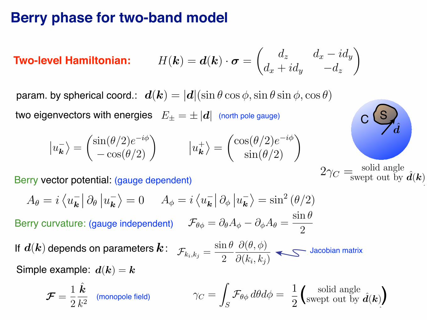
Fki,kj =sin

2

(,)

(ki, kj)(2)

k d(k) (3)

F = A A =sin

2(4)

Berry vector potential

A = iuk

uk

= 0 (5)

A = iuk

uk

= sin2 (/2) (6)

and

A = (7)u+

k

=

cos(/2)ei

sin(/2)

(8)

uk

=

sin(/2)ei

cos(/2)

(9)

(10)

E± = ± |d| (11)

and this

d(k) = |d|(sin cos , sin sin , cos ) (12)

H(k) = d(k) · =

dz dx idy

dx + idy dz

(13)

and

2 (14)

kg |u(k)

g U(1)

(15)

22s (E = 0.6)

ijs 1/

|q| 2E/t (16)

and this

gk = kzz

+(kx + ky)(x + y) (17)

For 3D:

Festk

¨


¨

osung 11.


Simple example

d(k) = k (1)

C =

S

F · dk (2)

Berry curvature tensor

Fµ(k) =

kµA(k)

kAµ(k) (3)

Berry curvature

Fki,kj =sin

2

(,)

(ki, kj)(4)

k d(k) (5)

F = A A =sin

2(6)


A = iuk

uk

= 0 (7)

A = iuk

uk

= sin2 (/2) (8)

and

A = (9)u+

k

=

cos(/2)ei

sin(/2)

(10)

uk

=

sin(/2)ei

cos(/2)

(11)

(12)

E± = ± |d| (13)

and this


H(k) = d(k) · =

dz dx idy

dx + idy dz

(15)

and

2 (16)

kg |u(k)

g U(1)

(17)

22s (E = 0.6)

ijs 1/

|q| 2E/t (18)

Festk

¨


¨

osung 11.


Simple example

Fµ = µF (1)

F = k A (2)

d(k) = k (3)

C =

S

F · dk (4)


Fµ(k) =

kµA(k)

kAµ(k) (5)

Berry curvature

Fki,kj =sin

2

(,)

(ki, kj)(6)

k d(k) (7)

F = A A =sin

2(8)


A = iuk

uk

= 0 (9)

A = iuk

uk

= sin2 (/2) (10)

and

A = (11)u+

k

=

cos(/2)ei

sin(/2)

(12)

uk

=

sin(/2)ei

cos(/2)

(13)

(14)

E± = ± |d| (15)

and this


H(k) = d(k) · =

dz dx idy

dx + idy dz

(17)

Festk

¨


¨

osung 11.


Simple example

Fµ = µF (1)

F = k A (2)

d(k) = k (3)

C =

S

F · dk (4)


Fµ(k) =

kµA(k)

kAµ(k) (5)

Berry curvature

Fki,kj =sin

2

(,)

(ki, kj)(6)

k d(k) (7)

F = A A =sin

2(8)


A = iuk

uk

= 0 (9)

A = iuk

uk

= sin2 (/2) (10)

and

A = (11)u+

k

=

cos(/2)ei

sin(/2)

(12)

uk

=

sin(/2)ei

cos(/2)

(13)

(14)

E± = ± |d| (15)

and this


H(k) = d(k) · =

dz dx idy

dx + idy dz

(17)

Festk

¨


¨

osung 11.


Simple example

F =1

2

k

k2(1)

C =

S

F dd = (2)

Fµ = µF (3)

F = k A (4)

d(k) = k (5)

C =

S

F · dk (6)


Fµ(k) =

kµA(k)

kAµ(k) (7)

Berry curvature

Fki,kj =sin

2

(,)

(ki, kj)(8)

k d(k) (9)

F = A A =sin

2(10)


A = iuk

uk

= 0 (11)

A = iuk

uk

= sin2 (/2) (12)

and

A = (13)u+

k

=

cos(/2)ei

sin(/2)

(14)

uk

=

sin(/2)ei

cos(/2)

(15)

(16)

E± = ± |d| (17)

and this


H(k) = d(k) · =

dz dx idy

dx + idy dz

(19)

Festk

¨


¨

osung 11.



A = iuk

uk

= 0 (1)

A = iuk

uk

= sin2 (/2) (2)

and

A = (3)u+

k

=

cos(/2)ei

sin(/2)

(4)

uk

=

sin(/2)ei

cos(/2)

(5)

(6)

E± = ± |d| (7)

and this


H(k) = d(k) · =

dz dx idy

dx + idy dz

(9)

and

2 (10)

kg |u(k)

g U(1)

(11)

22s (E = 0.6)

ijs 1/

↵|q| 2E/t (12)

and this

gk = kzz

+(kx + ky)(x + y) (13)

some more

kx kz (14)


s i, j 1, 2, 3 (15)

s (E,q) = 1

d2k(2)2

Tr

SG(0)(E,k + q)V G0(E,k)

11

(16)

qx qy (17)

0s i

s , i 1, 2, 3 = 0 1, 2, 3 (18)

Festk

¨


¨

osung 11.


and

A = (1)u+

k

=

cos(/2)ei

sin(/2)

(2)

uk

=

sin(/2)ei

cos(/2)

(3)

(4)

E± = ± |k| (5)

and this

d(k) = k = |k|(sin cos , sin sin , cos ) (6)

H(k) = d(k) · =

dz dx idy

dx + idy dz

(7)

and

2 (8)

kg |u(k)

g U(1)

(9)

22s (E = 0.6)

ijs 1/

|q| 2E/t (10)

and this

gk = kzz

+(kx + ky)(x + y) (11)

some more

kx kz (12)


s i, j 1, 2, 3 (13)

s (E,q) = 1

d2k(2)2

Tr

SG(0)(E,k + q)V G0(E,k)

11

(14)

qx qy (15)

0s i

s , i 1, 2, 3 = 0 1, 2, 3 (16)

and this is it:

s (E,q) = 1

2i

(E,q)

(E,q)

↵, (17)

Festk

¨


¨

osung 11.


and

A = (1)u+

k

=

cos(/2)ei

sin(/2)

(2)

uk

=

sin(/2)ei

cos(/2)

(3)

(4)

E± = ± |k| (5)

and this


H(k) = d(k) · =

dz dx idy

dx + idy dz

(7)

and

2 (8)

kg |u(k)

g U(1)

(9)

22s (E = 0.6)

ijs 1/

|q| 2E/t (10)

and this

gk = kzz

+(kx + ky)(x + y) (11)

some more

kx kz (12)


s i, j 1, 2, 3 (13)

s (E,q) = 1

d2k(2)2

Tr

SG(0)(E,k + q)V G0(E,k)

11

(14)

qx qy (15)

0s i

s , i 1, 2, 3 = 0 1, 2, 3 (16)

and this is it:

s (E,q) = 1

2i

(E,q)

(E,q)

↵, (17)

Berry curvature: (gauge independent)

Berry phase for two-band model

Two-level Hamiltonian:

Simple example:

C S



and

H(k) = d(k) · σ d (1)

n =i

2π

!

"

Fd2k (2)

|u(k)⟩ → eiφk |u(k)⟩ (3)

A → A + ∇kφk (4)

F = ∇k ×A (5)

γC =

#

C

A · dk (6)

γC =

"

S

Fd2k (7)

=⇒ (8)

Bloch theorem

[T (R), H ] = 0 k |ψn⟩ = eikr |un(k)⟩ (9)

(10)


(12)

H(k) |un(k)⟩ = En(k) |un(k)⟩ (13)

we have


majoranas

γ1 = ψ + ψ† (15)

γ2 = −i$

ψ − ψ†%

(16)

and

ψ = γ1 + iγ2 (17)

ψ† = γ1 − iγ2 (18)

and

γ2i = 1 (19)

γi, γj = 2δij (20)

Festk

¨


¨

osung 11.


and this

H(k) = d(k) · =

dz dx idy

dx + idy dz

(1)

and

2 (2)

kg |u(k)

g U(1)

(3)

22s (E = 0.6)

ijs 1/

|q| 2E/t (4)

and this

gk = kzz

+(kx + ky)(x + y) (5)

some more

kx kz (6)


s i, j 1, 2, 3 (7)

s (E,q) = 1

d2k

(2)2Tr

SG(0)(E,k + q)V G0(E,k)

11

(8)

qx qy (9)

0s i

s , i 1, 2, 3 = 0 1, 2, 3 (10)

and this is it:

s (E,q) = 1

2i

(E,q)

(E,q)

↵, (11)

and

Gnn(E,k,q) =

nn

G(0)nn(E,k

)VnnG

(0)nn(E,k), (12)

and

(E,q) =

d2k

(2)2Tr

SG(0)(E,k + q)V G0(E,k)

11

. (13)


q = kf ki kf ki = 2/|q| (14)

two eigenvectors with energies

param. by spherical coord.:

Berry vector potential: (gauge dependent)

(north pole gauge)

Festk

¨


¨

osung 11.



A = iuk

uk

= 0 (1)

A = iuk

uk

= sin (/2)2 (2)

and

A = (3)u+

k

=

cos(/2)ei

sin(/2)

(4)

uk

=

sin(/2)ei

cos(/2)

(5)

(6)

E± = ± |k| (7)

and this


H(k) = d(k) · =

dz dx idy

dx + idy dz

(9)

and

2 (10)

kg |u(k)

g U(1)

(11)

22s (E = 0.6)

ijs 1/

↵|q| 2E/t (12)

and this

gk = kzz

+(kx + ky)(x + y) (13)

some more

kx kz (14)


s i, j 1, 2, 3 (15)

s (E,q) = 1

d2k(2)2

Tr

SG(0)(E,k + q)V G0(E,k)

11

(16)

qx qy (17)

0s i

s , i 1, 2, 3 = 0 1, 2, 3 (18)

Festk

¨


¨

osung 11.



A = iuk

uk

= 0 (1)

A = iuk

uk

= sin (/2)2 (2)

and

A = (3)u+

k

=

cos(/2)ei

sin(/2)

(4)

uk

=

sin(/2)ei

cos(/2)

(5)

(6)

E± = ± |k| (7)

and this


H(k) = d(k) · =

dz dx idy

dx + idy dz

(9)

and

2 (10)

kg |u(k)

g U(1)

(11)

22s (E = 0.6)

ijs 1/

↵|q| 2E/t (12)

and this

gk = kzz

+(kx + ky)(x + y) (13)

some more

kx kz (14)


s i, j 1, 2, 3 (15)

s (E,q) = 1

d2k(2)2

Tr

SG(0)(E,k + q)V G0(E,k)

11

(16)

qx qy (17)

0s i

s , i 1, 2, 3 = 0 1, 2, 3 (18)

Festk

¨


¨

osung 11.



A = iuk

uk

= 0 (1)

A = iuk

uk

= sin (/2)2 (2)

and

A = (3)u+

k

=

cos(/2)ei

sin(/2)

(4)

uk

=

sin(/2)ei

cos(/2)

(5)

(6)

E± = ± |d| (7)

and this


H(k) = d(k) · =

dz dx idy

dx + idy dz

(9)

and

2 (10)

kg |u(k)

g U(1)

(11)

22s (E = 0.6)

ijs 1/

↵|q| 2E/t (12)

and this

gk = kzz

+(kx + ky)(x + y) (13)

some more

kx kz (14)


s i, j 1, 2, 3 (15)

s (E,q) = 1

d2k(2)2

Tr

SG(0)(E,k + q)V G0(E,k)

11

(16)

qx qy (17)

0s i

s , i 1, 2, 3 = 0 1, 2, 3 (18)

If depends on parameters :

Festk

¨


¨

osung 11.


Berry curvature

d(k) (1)

F = A A =sin

2(2)


A = iuk

uk

= 0 (3)

A = iuk

uk

= sin2 (/2) (4)

and

A = (5)u+

k

=

cos(/2)ei

sin(/2)

(6)

uk

=

sin(/2)ei

cos(/2)

(7)

(8)

E± = ± |d| (9)

and this


H(k) = d(k) · =

dz dx idy

dx + idy dz

(11)

and

2 (12)

kg |u(k)

g U(1)

(13)

22s (E = 0.6)

ijs 1/

↵|q| 2E/t (14)

and this

gk = kzz

+(kx + ky)(x + y) (15)

some more

kx kz (16)


s i, j 1, 2, 3 (17)

s (E,q) = 1

d2k(2)2

Tr

SG(0)(E,k + q)V G0(E,k)

11

(18)

qx qy (19)

0s i

s , i 1, 2, 3 = 0 1, 2, 3 (20)

Festk

¨


¨

osung 11.


Berry curvature

k d(k) (1)

F = A A =sin

2(2)


A = iuk

uk

= 0 (3)

A = iuk

uk

= sin2 (/2) (4)

and

A = (5)u+

k

=

cos(/2)ei

sin(/2)

(6)

uk

=

sin(/2)ei

cos(/2)

(7)

(8)

E± = ± |d| (9)

and this


H(k) = d(k) · =

dz dx idy

dx + idy dz

(11)

and

2 (12)

kg |u(k)

g U(1)

(13)

22s (E = 0.6)

ijs 1/

↵|q| 2E/t (14)

and this

gk = kzz

+(kx + ky)(x + y) (15)

some more

kx kz (16)


s i, j 1, 2, 3 (17)

s (E,q) = 1

d2k(2)2

Tr

SG(0)(E,k + q)V G0(E,k)

11

(18)

qx qy (19)

0s i

s , i 1, 2, 3 = 0 1, 2, 3 (20)

Jacobian matrix

Festk

¨


¨

osung 11.


Simple example

d(k) = k (1)

C =

S

F · dk (2)

Berry curvature

Fki,kj =sin

2

(,)

(ki, kj)(3)

k d(k) (4)

F = A A =sin

2(5)


A = iuk

uk

= 0 (6)

A = iuk

uk

= sin2 (/2) (7)

and

A = (8)u+

k

=

cos(/2)ei

sin(/2)

(9)

uk

=

sin(/2)ei

cos(/2)

(10)

(11)

E± = ± |d| (12)

and this


H(k) = d(k) · =

dz dx idy

dx + idy dz

(14)

and

2 (15)

kg |u(k)

g U(1)

(16)

22s (E = 0.6)

ijs 1/

|q| 2E/t (17)



and

2γC = Solid angle swept out by d(k) (1)

H(k) = d(k) · σ d (2)

n =i

2π

!

"

Fd2k (3)

|u(k)⟩ → eiφk |u(k)⟩ (4)

A → A + ∇kφk (5)

F = ∇k ×A (6)

γC =

#

C

A · dk (7)

γC =

"

S

Fd2k (8)

=⇒ (9)

Bloch theorem

[T (R), H ] = 0 k |ψn⟩ = eikr |un(k)⟩ (10)

(11)


(13)

H(k) |un(k)⟩ = En(k) |un(k)⟩ (14)

we have


majoranas

γ1 = ψ + ψ† (16)

γ2 = −i$

ψ − ψ†%

(17)

and

ψ = γ1 + iγ2 (18)

ψ† = γ1 − iγ2 (19)

and

γ2i = 1 (20)

γi, γj = 2δij (21)



and

2γC = solid angle swept out by d(k) (1)

H(k) = d(k) · σ d (2)

n =i

2π

!

"

Fd2k (3)

|u(k)⟩ → eiφk |u(k)⟩ (4)

A → A + ∇kφk (5)

F = ∇k ×A (6)

γC =

#

C

A · dk (7)

γC =

"

S

Fd2k (8)

=⇒ (9)

Bloch theorem

[T (R), H ] = 0 k |ψn⟩ = eikr |un(k)⟩ (10)

(11)


(13)

H(k) |un(k)⟩ = En(k) |un(k)⟩ (14)

we have


majoranas

γ1 = ψ + ψ† (16)

γ2 = −i$

ψ − ψ†%

(17)

and

ψ = γ1 + iγ2 (18)

ψ† = γ1 − iγ2 (19)

and

γ2i = 1 (20)

γi, γj = 2δij (21)



and


H(k) = d(k) · σ d (2)

n =i

2π

!

"

Fd2k (3)

|u(k)⟩ → eiφk |u(k)⟩ (4)

A → A + ∇kφk (5)

F = ∇k ×A (6)

γC =

#

C

A · dk (7)

γC =

"

S

Fd2k (8)

=⇒ (9)

Bloch theorem

[T (R), H ] = 0 k |ψn⟩ = eikr |un(k)⟩ (10)

(11)


(13)

H(k) |un(k)⟩ = En(k) |un(k)⟩ (14)

we have


majoranas

γ1 = ψ + ψ† (16)

γ2 = −i$

ψ − ψ†%

(17)

and

ψ = γ1 + iγ2 (18)

ψ† = γ1 − iγ2 (19)

and

γ2i = 1 (20)

γi, γj = 2δij (21)

(monopole field)

Festk

¨


¨

osung 11.


Simple example

C =

S

F dd = (1)

Fµ = µF (2)

F = k A (3)

d(k) = k (4)

C =

S

F · dk (5)


Fµ(k) =

kµA(k)

kAµ(k) (6)

Berry curvature

Fki,kj =sin

2

(,)

(ki, kj)(7)

k d(k) (8)

F = A A =sin

2(9)


A = iuk

uk

= 0 (10)

A = iuk

uk

= sin2 (/2) (11)

and

A = (12)u+

k

=

cos(/2)ei

sin(/2)

(13)

uk

=

sin(/2)ei

cos(/2)

(14)

(15)

E± = ± |d| (16)

and this


H(k) = d(k) · =

dz dx idy

dx + idy dz

(18)



and


H(k) = d(k) · σ d (2)

n =i

2π

!

"

Fd2k (3)

|u(k)⟩ → eiφk |u(k)⟩ (4)

A → A + ∇kφk (5)

F = ∇k ×A (6)

γC =

#

C

A · dk (7)

γC =

"

S

Fd2k (8)

=⇒ (9)

Bloch theorem

[T (R), H ] = 0 k |ψn⟩ = eikr |un(k)⟩ (10)

(11)


(13)

H(k) |un(k)⟩ = En(k) |un(k)⟩ (14)

we have


majoranas

γ1 = ψ + ψ† (16)

γ2 = −i$

ψ − ψ†%

(17)

and

ψ = γ1 + iγ2 (18)

ψ† = γ1 − iγ2 (19)

and

γ2i = 1 (20)

γi, γj = 2δij (21)



and


H(k) = d(k) · σ d (2)

n =i

2π

!

"

Fd2k (3)

|u(k)⟩ → eiφk |u(k)⟩ (4)

A → A + ∇kφk (5)

F = ∇k ×A (6)

γC =

#

C

A · dk (7)

γC =

"

S

Fd2k (8)

=⇒ (9)

Bloch theorem

[T (R), H ] = 0 k |ψn⟩ = eikr |un(k)⟩ (10)

(11)


(13)

H(k) |un(k)⟩ = En(k) |un(k)⟩ (14)

we have


majoranas

γ1 = ψ + ψ† (16)

γ2 = −i$

ψ − ψ†%

(17)

and

ψ = γ1 + iγ2 (18)

ψ† = γ1 − iγ2 (19)

and

γ2i = 1 (20)

γi, γj = 2δij (21)

( )1

2

Festk

¨


¨

osung 11.


Simple example

F =1

2

k

k2(1)

C =

S

F dd = (2)

Fµ = µF (3)

F = k A (4)

d(k) = k (5)

C =

S

F · dk (6)


Fµ(k) =

kµA(k)

kAµ(k) (7)

Berry curvature

Fki,kj =sin

2

(,)

(ki, kj)(8)

k d(k) (9)

F = A A =sin

2(10)


A = iuk

uk

= 0 (11)

A = iuk

uk

= sin2 (/2) (12)

and

A = (13)u+

k

=

cos(/2)ei

sin(/2)

(14)

uk

=

sin(/2)ei

cos(/2)

(15)

(16)

E± = ± |d| (17)

and this


H(k) = d(k) · =

dz dx idy

dx + idy dz

(19)

Festk

¨


¨

osung 11.


Simple example

F =1

2

k

k2(1)

C =

S

F dd = (2)

Fµ = µF (3)

F = k A (4)

d(k) = k (5)

C =

S

F · dk (6)


Fµ(k) =

kµA(k)

kAµ(k) (7)

Berry curvature

Fki,kj =sin

2

(,)

(ki, kj)(8)

k d(k) (9)

F = A A =sin

2(10)


A = iuk

uk

= 0 (11)

A = iuk

uk

= sin2 (/2) (12)

and

A = (13)u+

k

=

cos(/2)ei

sin(/2)

(14)

uk

=

sin(/2)ei

cos(/2)

(15)

(16)

E± = ± |d| (17)

and this


H(k) = d(k) · =

dz dx idy

dx + idy dz

(19)

Polyacetylene (Su-Schrieffer-Heeger model)

Su-Schrieffer-Heeger model describes polyacetylene

Festk

¨


¨

osung 11.


Simple example

[C2H2]n (1)

F =1

2

k

k2(2)

C =

S

F dd = (3)

Fµ = µF (4)

F = k A (5)

d(k) = k (6)

C =

S

F · dk (7)


Fµ(k) =

kµA(k)

kAµ(k) (8)

Berry curvature

Fki,kj =sin

2

(,)

(ki, kj)(9)

k d(k) (10)

F = A A =sin

2(11)


A = iuk

uk

= 0 (12)

A = iuk

uk

= sin2 (/2) (13)

and

A = (14)u+

k

=

cos(/2)ei

sin(/2)

(15)

uk

=

sin(/2)ei

cos(/2)

(16)

(17)

E± = ± |d| (18)

and this


H(k) = d(k) · =

dz dx idy

dx + idy dz

(20)

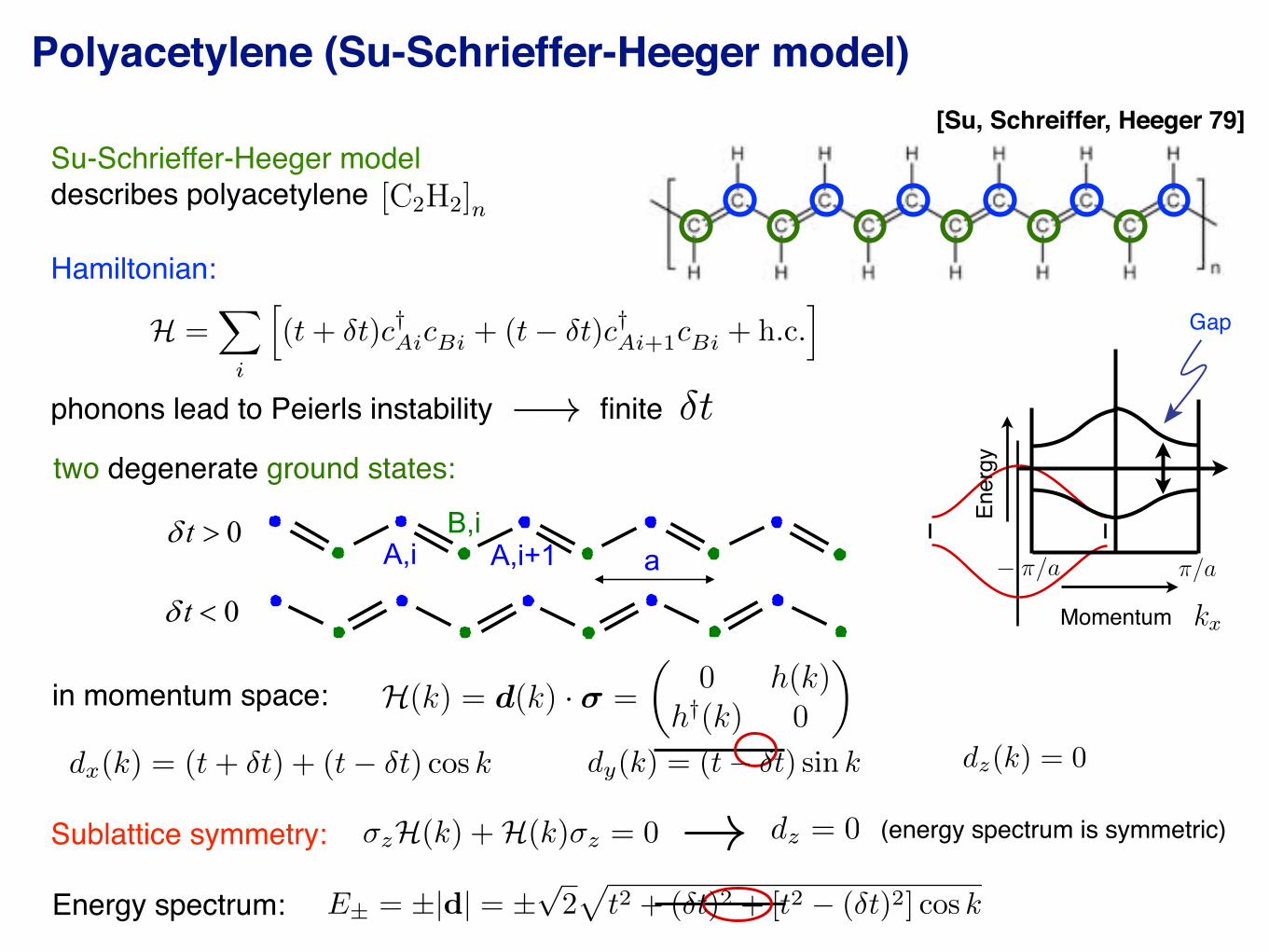
Hamiltonian:

two degenerate ground states:

H =X

i

h(t+ t)c†AicBi + (t t)c†Ai+1cBi + h.c.

i

Su Schrieffer Heeger Model model for polyacetalenesimplest “two band” model

† †1( ) ( ) . .Ai Bi Ai Bi

i

H t t c c t t c c h c

( ) ( )H k k d

( ) ( ) ( ) cos

( ) ( )sin

( ) 0

x

y

z

d k t t t t ka

d k t t ka

d k

0t

0t

a

d(k)

d(k)

dx

dy

dx

dy

E(k)

k

/a/a

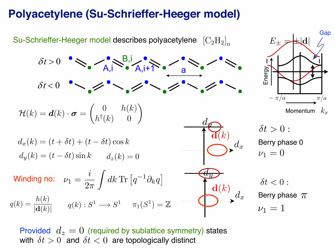
Provided symmetry requires dz(k)=0, the states with t>0 and t<0 are topologically distinct.Without the extra symmetry, all 1D band structures are topologically equivalent.

A,iB,i

t>0 : Berry phase 0

P = 0

t<0 : Berry phase P = e/2

Gap 4|t|

Peierl’s instability t

A,i+1

phonons lead to Peierls instability finite

!

t

in momentum space:

Sublattice symmetry:

Energy spectrum:

dx

(k) = (t+ t) + (t t) cos k

Festk

¨


¨

osung 11.


Simple example Polyacethylene:

H(k) = d(k) · =

0 h(k)

h†(k) 0

(1)

and

[C2H2]n (2)

F =1

2

k

k2(3)

C =

S

F dd = (4)

Fµ = µF (5)

F = k A (6)

d(k) = k (7)

C =

S

F · dk (8)


Fµ(k) =

kµA(k)

kAµ(k) (9)

Berry curvature

Fki,kj =sin

2

(,)

(ki, kj)(10)

k d(k) (11)

F = A A =sin

2(12)


A = iuk

uk

= 0 (13)

A = iuk

uk

= sin2 (/2) (14)

and

A = (15)u+

k

=

cos(/2)ei

sin(/2)

(16)

uk

=

sin(/2)ei

cos(/2)

(17)

(18)

E± = ± |d| (19)

dy(k) = (t t) sin k dz(k) = 0



we have


majoranas

γ1 = ψ + ψ† (2)

γ2 = −i!

ψ − ψ†"

(3)

and

ψ = γ1 + iγ2 (4)

ψ† = γ1 − iγ2 (5)

and

γ2i = 1 (6)


mean field

γ†E=0 = γE=0 (8)

⇒ γ†k,E = γ−k,−E (9)

Ξ ψ+k,+E = τxψ∗−k,−E (10)

Ξ2 = +1 Ξ = τxK (11)

τx =

#

0 11 0

$

(12)

c†c c†c ⇒ ⟨c†c†⟩c c = ∆∗c c (13)

weak vs strong

|µ| < 4t (14)

n = 1 (15)


m(k) =m(k)

|m(k)|m(k) : m(k) ∈ S2 π2(S

2) = (16)


mx my mz (18)



we have


majoranas

γ1 = ψ + ψ† (2)

γ2 = −i!

ψ − ψ†"

(3)

and

ψ = γ1 + iγ2 (4)

ψ† = γ1 − iγ2 (5)

and

γ2i = 1 (6)


mean field

γ†E=0 = γE=0 (8)

⇒ γ†k,E = γ−k,−E (9)

Ξ ψ+k,+E = τxψ∗−k,−E (10)

Ξ2 = +1 Ξ = τxK (11)

τx =

#

0 11 0

$

(12)

c†c c†c ⇒ ⟨c†c†⟩c c = ∆∗c c (13)

weak vs strong

|µ| < 4t (14)

n = 1 (15)


m(k) =m(k)

|m(k)|m(k) : m(k) ∈ S2 π2(S

2) = (16)


mx my mz (18)

Ener

gy

Momentum



homotopy

ν = # kx (1)

∆±k

= ∆s ± ∆t |dk| (2)

∆s > ∆t ∆s ∼ ∆t ν = ±1 for ∆t > ∆s (3)

and

π3[U(2)] = q(k) :∈ U(2) (4)

Lattice BdG HBdG

h(k) = εkσ0 + αgk · σ (5)

∆(k) = (∆sσ0 + ∆tdk · σ) iσy (6)

hex Iy ≃e

!

! kF,−

kF,+

dky

2πsgn

"

#

µ

Hµexρ

µ1 (0, ky)

$

%


n=1

ρxn(0, ky) cos ky

&

.(7)

and

jn,ky = −t sin ky

'


cnky↓

(

(8)

+ λ cos ky

'


(

(9)




)

)ψl,ky

*

of H(10)ky

,

Iy = −e

!

1

Ny

#

ky

Lx/2#

n=1

#

l,El<0




∝3

#

µ=1

Hµexρ

µ1 (E, ky) ρx

1 (11)

NQPI(ω, q) = −1

πIm

+

#

k

G0(k, ω)T (ω)G0(k + q, ω)

,

∝-

Sf

)

)

)T (ω)

)

)

)Si

.

(12)

a (13)

ξ±k

= εk ± α |gk|(14)

Gap

E± = ±|d| = ±2

pt2 + (t)2 + [t2 (t)2] cos k

(energy spectrum is symmetric)

!

dz = 0zH(k) +H(k)z = 0

[Su, Schreiffer, Heeger 79]

Polyacetylene (Su-Schrieffer-Heeger model)

Su-Schrieffer-Heeger model describes polyacetylene

Festk

¨


¨

osung 11.


Simple example

[C2H2]n (1)

F =1

2

k

k2(2)

C =

S

F dd = (3)

Fµ = µF (4)

F = k A (5)

d(k) = k (6)

C =

S

F · dk (7)


Fµ(k) =

kµA(k)

kAµ(k) (8)

Berry curvature

Fki,kj =sin

2

(,)

(ki, kj)(9)

k d(k) (10)

F = A A =sin

2(11)


A = iuk

uk

= 0 (12)

A = iuk

uk

= sin2 (/2) (13)

and

A = (14)u+

k

=

cos(/2)ei

sin(/2)

(15)

uk

=

sin(/2)ei

cos(/2)

(16)

(17)

E± = ± |d| (18)

and this


H(k) = d(k) · =

dz dx idy

dx + idy dz

(20)

Su Schrieffer Heeger Model model for polyacetalenesimplest “two band” model

† †1( ) ( ) . .Ai Bi Ai Bi

i

H t t c c t t c c h c

( ) ( )H k k d

( ) ( ) ( ) cos

( ) ( )sin

( ) 0

x

y

z

d k t t t t ka

d k t t ka

d k

0t

0t

a

d(k)

d(k)

dx

dy

dx

dy

E(k)

k

/a/a

Provided symmetry requires dz(k)=0, the states with t>0 and t<0 are topologically distinct.Without the extra symmetry, all 1D band structures are topologically equivalent.

A,iB,i

t>0 : Berry phase 0

P = 0

t<0 : Berry phase P = e/2

Gap 4|t|

Peierl’s instability t

A,i+1

Festk

¨


¨

osung 11.


Simple example Polyacethylene:

H(k) = d(k) · =

0 h(k)

h†(k) 0

(1)

and

[C2H2]n (2)

F =1

2

k

k2(3)

C =

S

F dd = (4)

Fµ = µF (5)

F = k A (6)

d(k) = k (7)

C =

S

F · dk (8)


Fµ(k) =

kµA(k)

kAµ(k) (9)

Berry curvature

Fki,kj =sin

2

(,)

(ki, kj)(10)

k d(k) (11)

F = A A =sin

2(12)


A = iuk

uk

= 0 (13)

A = iuk

uk

= sin2 (/2) (14)

and

A = (15)u+

k

=

cos(/2)ei

sin(/2)

(16)

uk

=

sin(/2)ei

cos(/2)

(17)

(18)

E± = ± |d| (19)

dx

(k) = (t+ t) + (t t) cos k

dy(k) = (t t) sin k dz(k) = 0



we have


majoranas

γ1 = ψ + ψ† (2)

γ2 = −i!

ψ − ψ†"

(3)

and

ψ = γ1 + iγ2 (4)

ψ† = γ1 − iγ2 (5)

and

γ2i = 1 (6)


mean field

γ†E=0 = γE=0 (8)

⇒ γ†k,E = γ−k,−E (9)

Ξ ψ+k,+E = τxψ∗−k,−E (10)

Ξ2 = +1 Ξ = τxK (11)

τx =

#

0 11 0

$

(12)

c†c c†c ⇒ ⟨c†c†⟩c c = ∆∗c c (13)

weak vs strong

|µ| < 4t (14)

n = 1 (15)


m(k) =m(k)

|m(k)|m(k) : m(k) ∈ S2 π2(S

2) = (16)


mx my mz (18)



we have


majoranas

γ1 = ψ + ψ† (2)

γ2 = −i!

ψ − ψ†"

(3)

and

ψ = γ1 + iγ2 (4)

ψ† = γ1 − iγ2 (5)

and

γ2i = 1 (6)


mean field

γ†E=0 = γE=0 (8)

⇒ γ†k,E = γ−k,−E (9)

Ξ ψ+k,+E = τxψ∗−k,−E (10)

Ξ2 = +1 Ξ = τxK (11)

τx =

#

0 11 0

$

(12)

c†c c†c ⇒ ⟨c†c†⟩c c = ∆∗c c (13)

weak vs strong

|µ| < 4t (14)

n = 1 (15)


m(k) =m(k)

|m(k)|m(k) : m(k) ∈ S2 π2(S

2) = (16)


mx my mz (18)

Ener

gy

Momentum



homotopy

ν = # kx (1)

∆±k

= ∆s ± ∆t |dk| (2)

∆s > ∆t ∆s ∼ ∆t ν = ±1 for ∆t > ∆s (3)

and

π3[U(2)] = q(k) :∈ U(2) (4)

Lattice BdG HBdG

h(k) = εkσ0 + αgk · σ (5)

∆(k) = (∆sσ0 + ∆tdk · σ) iσy (6)

hex Iy ≃e

!

! kF,−

kF,+

dky

2πsgn

"

#

µ

Hµexρ

µ1 (0, ky)

$

%


n=1

ρxn(0, ky) cos ky

&

.(7)

and

jn,ky = −t sin ky

'


cnky↓

(

(8)

+ λ cos ky

'


(

(9)




)

)ψl,ky

*

of H(10)ky

,

Iy = −e

!

1

Ny

#

ky

Lx/2#

n=1

#

l,El<0




∝3

#

µ=1

Hµexρ

µ1 (E, ky) ρx

1 (11)

NQPI(ω, q) = −1

πIm

+

#

k

G0(k, ω)T (ω)G0(k + q, ω)

,

∝-

Sf

)

)

)T (ω)

)

)

)Si

.

(12)

a (13)

ξ±k

= εk ± α |gk|(14)

GapE± = ±|d|

Provided (required by sublattice symmetry) states with and are topologically distinct

dz = 0t > 0 t < 0

dx

dyd(k)

t > 0 :Berry phase 0

dx

dy

d(k)t < 0 :

Berry phase

1 = 0

1 = 1

Winding no:

q(k) =h(k)

|d(k)| q(k) : S1 ! S1



1. f-Summenregel

Now we do the following

WS3 =1

24π2

!

S3

d2k dω εµνλTr"

G∂µG−1G∂νG−1G∂λG−1#

(1)

and

NS2 =1

2π

!

S2

d2k Tr [F ] F = ∇×A (2)

Time-reversal symmetry:

UTH∗(k)U †T = +H(−k), UT = σ0 (3)

Particle-hole symmetry: S = TC = σ2

UCH∗(k)U †C = −H(−k), UC = iσ2 (4)

basis in which S the H(k) Off-diagonal form

H(k) =

$

0 εk − i∆k

εk + i∆k 0

%

(5)

qk is

q(k) : S1 −→ S1 π1(S1) = (6)

Hintωres

Tc(x) =? = 5.4

ty > tx

qy = π

ω > ωres

ω = 40 meV

Energy [meV]new

1 =i

2

ZdkTr

q1@kq

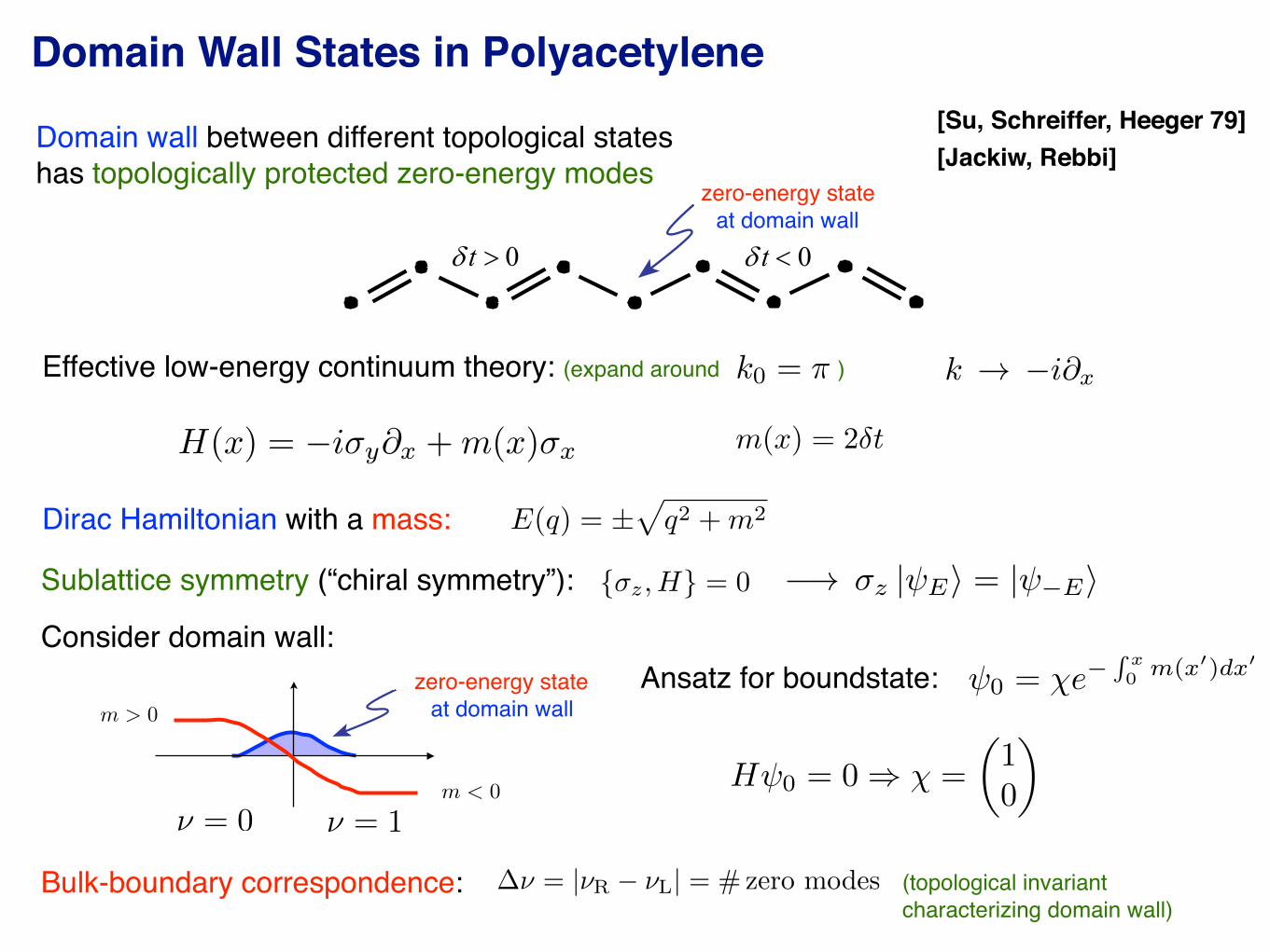
Domain Wall States in Polyacetylene

Domain wall between different topological states has topologically protected zero-energy modes

Effective low-energy continuum theory: (expand around )

Domain Wall StatesAn interface between different topological states has topologically protected midgap states

Low energy continuum theory :For small t focus on low energy states with k~/a xk q q i

a

;

( )vF x x yH i m x

0t 0t

Massive 1+1 D Dirac Hamiltonian

“Chiral” Symmetry :

2v ; F ta m t

, 0 z z E EH

0

( ') '/ v

0

1( )

0

x

Fm x dx

x e

Egap=2|m|Domain wall

bound state 0

m>0

m<0

2 2( ) ( )vFE q q m

Zero mode : topologically protected eigenstate at E=0(Jackiw and Rebbi 76, Su Schrieffer, Heeger 79)

Any eigenstate at +E has a partner at -E

zero-energy state at domain wall

Sublattice symmetry (“chiral symmetry”):

k0 = k ! ix

m(x) = 2t

Dirac Hamiltonian with a mass:

[Su, Schreiffer, Heeger 79]

E(q) = ±p

q2 +m2

z, H = 0 z | E = | EConsider domain wall:

m > 0

m < 0

zero-energy state at domain wall

[Jackiw, Rebbi]

Ansatz for boundstate:

Bulk-boundary correspondence: = |R L| = #zero modes (topological invariant characterizing domain wall)

= 1 = 0

0 = eR

x

0 m(x0)dx0

H(x) = iy

@x

+m(x)x

H 0 = 0 ) =

10

Documents

Modern Topics in Solid-State Theory: Topological ... · Modern Topics in Solid-State Theory: Topological insulators and superconductors Universität Stuttgart. 1. Topological band