1

Monetary compensations in climate policy

through the lens of a general equilibrium assessment

The case of oil-exporting countries

Henri WAISMAN*,# Julie ROZENBERG* and Jean Charles HOURCADE*

*Centre International de Recherche sur l’Environnement et le Développement

(CIRED, ParisTech/ENPC & CNRS/EHESS) –

45bis avenue de la Belle Gabrielle 94736 Nogent sur Marne CEDEX, France.

# Author for correspondence:

Phone: +33 1 4394 7378; Fax: +33 1 4394 7370; Email: waisman@centre-cired.fr.

2

Monetary compensations in climate policy

through the lens of a general equilibrium assessment:

The case of oil-exporting countries

ABSTRACT

This paper investigates the compensations that major oil producers have claimed for since the

Kyoto Protocol in order to alleviate the adverse impacts of climate policy on their economies.

The amount of these adverse impacts is assessed through a general equilibrium model which

endogenizes both the reduction of oil exportation revenues under international climate policy

and the macroeconomic effect of carbon pricing on Middle-East’s economy. We show that

compensating the drop of exportation revenues does not offset GDP and welfare losses

because of the time profile of the general equilibrium effects. When considering instead

compensation based on GDP losses, the effectiveness of monetary transfers proves to be

drastically limited by general equilibrium effects in opened economies. The main channels of

this efficiency gap are investigated and its magnitude proves to be conditional upon strategic

and policy choices of the Middle-East. This leads us to suggest that other means than direct

monetary compensating transfers should be discussed to engage the Middle-East in climate

policies.

Keywords: monetary transfers; oil exporters; climate policy

JEL classification: C68, Q32, Q54

3

Monetary compensations in climate policy

through the lens of a general equilibrium assessment:

The case of oil-exporting countries

The compensation of developing countries for the adverse impacts of climate change and

climate policies is one of the constant stumbling blocks of international climate negotiations.

These adverse impacts encompass three distinct issues: climate change damages, higher

energy prices affecting households’ purchase power and firms’ production costs and the

reduction of exportation revenues in fossil fuel producing economies. Historically, it is under

pressure of Middle-East countries and the Organization of the Petroleum-Exporting Countries

(OPEC) that these concerns have been officially acknowledged at different stages of

international negotiations, since article 4.8 of the UNFCCC1 and article 3.14 of the Kyoto

protocol2 (Barnett and Dessai, 2002) until, more recently, Article 1 of the 2009 Copenhagen

Agreement3.

This repetition is the sign that no tangible progress could be made about this sticking point of

climate negotiations in the past decades. This impasse has obvious political roots, i.e. the

reluctance of developed countries to grant large transfers towards countries perceived as rent

seekers, especially in a context of public budget constraint. But, beyond this political

dimension, compensations based on monetary transfers raise questions about both their

amount and their efficiency for sustaining economic activity in a general equilibrium vision.

This paper tries and frames these two sides of the compensation problem.

The first question relates to the evaluation of climate policy losses in oil-exporting countries,

which defines the compensations but remains a controversial topic in the literature. General

equilibrium energy-economy models predict significant costs4 whereas dynamic partial

equilibrium models find moderate losses5. These opposite conclusions are related to the

4

assumptions underlying the two approaches. The former conventionally assumes optimized

trajectories under perfect foresight and flexible technical and market adjustments, which

comes down to overlooking the potential co-benefits of climate policies permitted by the

correction of baseline sub-optimalities. The latter do not consider the feedback effects of the

oil sector on macroeconomic indicators and hence do not account for the reduction of world

oil demand under climate policy, a potentially major adverse impact on oil-exporting

economies. One ambition of this paper is thus to provide a comprehensive assessment of the

cost of climate policy in oil-exporting countries through a combination of these two

approaches, i.e. in a hybrid top-down/bottom-up framework (Hourcade et al, 2006).

The second question relates to the effect of monetary transfers on economic activity and

welfare in the recipient country, which has been investigated in a large body of literature on

the empirics of “development aid and growth”. A recent survey by (Doucouliagos and

Paldam, 2011) shows however that no univocal message can be derived from existing

assessments. Some support the idea that development aid promotes growth,6 whereas others

find it growth-neutral7 or even contributing to depress activity through indirect mechanisms

undermining aid effectiveness (Rajan and Subramanian, 2005). Among these, (Rajan and

Subramanian, 2011) typically demonstrate the role of real exchange rate overvaluation when

trade effects and structural lock-ins are accounted for. This mechanism is a source of the

‘natural resource curse’ through its negative effect on local competitiveness and socio-

economic development (e.g., Sachs and Warner, 2001; Frankel, 2010; Ross, 2012). It is a

particularly important dimension for the evaluation of monetary compensations in Middle-

East countries and it calls for endogenizing terms-of-trade adjustments..

We try and respond these two methodological challenges through a hybrid Computable

General Equilibrium (CGE) energy-economy model that captures the limited flexibility of

technical and economic adjustments under imperfect foresight, describes the domestic effects

5

of adjustments on the terms-of-trade and endogenizes long-run structural change in response

to price signals and geopolitical strategies (Section 1). This model is used to estimate the

socio-economic consequences of an international climate policy on oil markets and its adverse

impacts on Middle-East countries in terms of exportation revenues and macroeconomic

activity (Section 2). This assessment serves as a basis for estimating the monetary transfers

Middle-East countries may claim for in a climate policy context under two options depending

whether they compensate losses of oil revenue or of economic activity (Section 3). An

analytical study demonstrates that general equilibrium effects in a second-best setting create

the risk of an efficiency gap, i.e. that the ex-post benefit of transfers is lower than predicted

with an ex-ante calculation, and isolates its crucial determinants (Section 4). Finally,

numerical assessments confirm the relatively poor efficiency of monetary transfers to actually

sustain economic activity in Middle-East economies (Section 5). Section 6 concludes on the

implications of this analysis for international negotiations and, in particular, on the trap of

reducing the compensation problem in climate negotiations to a question of monetary

transfers.

1. Modelling long-term oil markets in a globalized economy

This paper adopts the IMACLIM-R model, which has been developed for the analysis of energy

and climate issues at a long-term horizon, and this section summarizes its specificities that are

of particular importance for the topics of this paper. 8

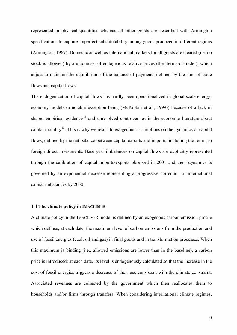
1.1 General structure of the IMACLIM-R model

IMACLIM-R is a recursive CGE model of the world economy, which endogenizes the interplay

between the dynamics of oil markets and the macroeconomy over the 2001-2050 period

through the recursive succession of annual static equilibria and dynamic modules (Figure 1).

6

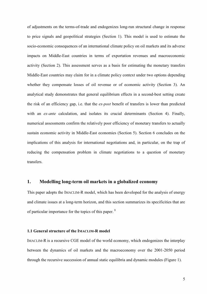
Figure 1: The recursive and modular structure of the IMACLIM-R model

The static equilibrium represents short-run macroeconomic interactions at each date t under

technology and capacity constraints. It is calculated assuming Leontief production functions

with fixed intermediate consumption, labour inputs and mark-up in non-energy sectors9.

Households maximize their utility through a tradeoff between consumption goods, mobility

services and residential energy uses considering fixed end-use equipment. Market clearing

conditions lead to a partial utilization of production capacities, given the fixed mark-up

pricing and the stickiness of labour markets. This equilibrium provides a snapshot of the

economy at date t in terms of relative prices, wages, employment, production levels and trade

flows.

The dynamic modules are reduced forms of bottom-up models, which describe the evolution

of structural and technical parameters between t and t+1 in response to past and current

economic signals. At each year, regional capital accumulation is given by firms’ investment,

households’ savings, and international capital flows. On that basis, the across-sector

distribution of investments is governed by expectations on sector profitability and technical

conditions as described in sector-specific reduced forms of technology-rich models (referred

to as Nexus modules and described in details in the Supplementary Material of (Waisman et

Updated parameters

(technical coefficients,

population, productivity)

Economic signals

(prices, quantities,

Investments)

Static Equilibrium (t)

under constraints

Agricolture

Energy

Transport

Bottom-up sub-models

(reduced forms

Static Equilibrium (t+1)

under updated constraints

Electricity

Oil

...

Industry

Transport

TIME PATH

7

al, 2012)). The Nexus modules represent the evolution of technical coefficients resulting from

agents’ microeconomic decisions on technological choices, given the limits imposed by the

innovation possibility frontier including a) sector-based information of economies of scale,

learning-by-doing mechanisms and saturation in efficiency progress, and b) expert views

about the asymptotes on ultimate technical potentials, the impact of incentive systems, and the

role of market or institutional imperfections. The new investment choices and technical

coefficients are then sent back to the static module in the form of updated production

capacities and input-output coefficients to calculate the t+1 equilibrium.

This structure comes to adopt a standard putty-clay representation with fixed technical content

of installed capital, which allows distinguishing between short-term rigidities and long-term

flexibilities (Johansen, 1959).10 The consistency of the iteration between the static

equilibrium and dynamic modules relies on ‘hybrid matrices’, which ensure an explicit

representation of the material and technical content of production processes through a

description of the economy in consistent money values and physical quantities (Sands et al.,

2005). In this multisectoral framework with partial use of production factors, market

imperfections and adaptive expectations, growth patterns may endogenously depart from the

natural rate given by exogenous assumptions on active population and labour productivity

(Phelps, 1961).

1.2 Description of oil markets

The description of oil supply in the IMACLIM-R model captures three crucial determinants of

oil exploitation at different time horizons (Rehrl and Friedrich, 2006):

• heterogeneous (conventional and non-conventional) oil reserves distinguished by their

exploitation cost, expressed in dollars per barrel ($/bbl);

8

• geological constraints limiting the short-term adaptability of oil supply and its long-term

availability;

• the market power of Middle-East countries and their ability to influence world oil prices

through their production decisions.11

In addition, macroeconomic interplays in IMACLIM-R include lessons from econometric

studies on the macroeconomic effects of the first oil shock (Hamilton, 2008). We incorporate

five model specifications that have been proven as necessary to reproduce the observed

magnitudes of macroeconomic effects consecutive to oil price variations:

• mark-up pricing to capture market imperfections (Rotemberg and Woodford, 1996);

• partial utilization rate of capital due to limits in the substitution between capital and

energy (Finn, 2000);

• a putty-clay description of technologies to represent the inertias of capital stock

(Atkeson and Kehoe, 1999);

• frictions in the reallocation of capital across heterogeneous sectors causing

differentiated levels of idle production capacities (Bresnahan and Ramey, 1993);

• frictions in the reallocation of labor across heterogeneous sectors causing

differentiated levels of unemployment (Davis and Haltiwanger, 2001).

The empirical evidence behind these two groups of model specifications and the

implementation of these principles into the IMACLIM-R are more extensively discussed in

(Waisman et al, 2012b).

1.3 Specifications for international trade

In IMACLIM-R, all intermediate and final goods are internationally tradable and total demand

for each good is satisfied by a mix of domestic production and imports. Energy flows are

9

represented in physical quantities whereas all other goods are described with Armington

specifications to capture imperfect substitutability among goods produced in different regions

(Armington, 1969). Domestic as well as international markets for all goods are cleared (i.e. no

stock is allowed) by a unique set of endogenous relative prices (the ‘terms-of-trade’), which

adjust to maintain the equilibrium of the balance of payments defined by the sum of trade

flows and capital flows.

The endogenization of capital flows has hardly been operationalized in global-scale energy-

economy models (a notable exception being (McKibbin et al., 1999)) because of a lack of

shared empirical evidence12 and unresolved controversies in the economic literature about

capital mobility13. This is why we resort to exogenous assumptions on the dynamics of capital

flows, defined by the net balance between capital exports and imports, including the return to

foreign direct investments. Base year imbalances on capital flows are explicitly represented

through the calibration of capital imports/exports observed in 2001 and their dynamics is

governed by an exponential decrease representing a progressive correction of international

capital imbalances by 2050.

1.4 The climate policy in IMACLIM-R

A climate policy in the IMACLIM-R model is defined by an exogenous carbon emission profile

which defines, at each date, the maximum level of carbon emissions from the production and

use of fossil energies (coal, oil and gas) in final goods and in transformation processes. When

this maximum is binding (i.e., allowed emissions are lower than in the baseline), a carbon

price is introduced: at each date, its level is endogenously calculated so that the increase in the

cost of fossil energies triggers a decrease of their use consistent with the climate constraint.

Associated revenues are collected by the government which then reallocates them to

households and/or firms through transfers. When considering international climate regimes,

10

international permit market can be modeled by defining regional allocations and introducing

transfers according to the difference between these and real emissions.

2. Oil markets and the costs of climate policy

In this section, we consider the ‘ideal’ case of a world agreement on a Kyoto-type climate

architecture with full participation, including the free compliance of Middle-East countries14.

Although this assumption may seem unrealistic, this scenario defines a useful benchmark to

assess the adverse impacts of a climate policy on major oil producers.

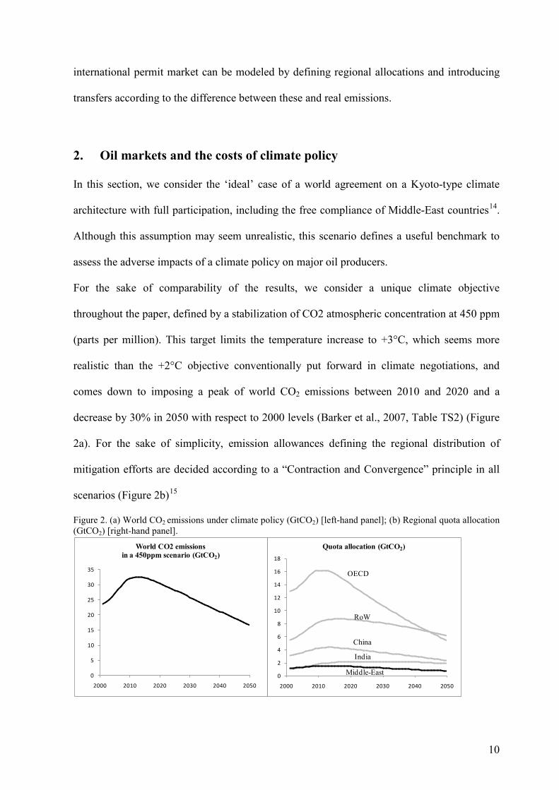
For the sake of comparability of the results, we consider a unique climate objective

throughout the paper, defined by a stabilization of CO2 atmospheric concentration at 450 ppm

(parts per million). This target limits the temperature increase to +3°C, which seems more

realistic than the +2°C objective conventionally put forward in climate negotiations, and

comes down to imposing a peak of world CO2 emissions between 2010 and 2020 and a

decrease by 30% in 2050 with respect to 2000 levels (Barker et al., 2007, Table TS2) (Figure

2a). For the sake of simplicity, emission allowances defining the regional distribution of

mitigation efforts are decided according to a “Contraction and Convergence” principle in all

scenarios (Figure 2b)15

Figure 2. (a) World CO2 emissions under climate policy (GtCO2) [left-hand panel]; (b) Regional quota allocation (GtCO2) [right-hand panel].

0

2

4

6

8

10

12

14

16

18

2000 2010 2020 2030 2040 2050

Quota allocation (GtCO2)

0

5

10

15

20

25

30

35

2000 2010 2020 2030 2040 2050

World CO2 emissions

in a 450ppm scenario (GtCO2)

OECD

India

China

RoW

Middle-East

11

For the sake of simplicity, we assume common assumptions on all the technical and

behavioral determinants of energy-economy trajectories, but sensitivity of model outcomes to

these assumptions are studied in other specific papers16. The only variant concerns oil price

trajectories, about which the literature on the strategic response of OPEC to various profiles of

carbon prices often concludes that major oil producers would adopt a limited deployment of

production capacities (IPCC, 2001, section 8.3.2.3). The rationale behind such behavior is to

cut back production to trigger price increases and hence maintain revenues despite the drop of

oil consumption (e.g., Berg and al., 1997b). However, low short-term oil prices may also have

some advantages in a climate policy context by simultaneously accelerating short-term oil

consumption and limiting the incentive for oil-free technical change to sustain long-term oil

demand. This is why we consider two oil pricing trajectories mimicking alternative reactions

of Middle-East producers:

- The Limited Deployment scenario (LD): Middle-East producers refrain from investing

in new capacity and maintain the medium term oil price around phigh=90$/bbl. This scenario

follows the standard conclusion of high prices permitting to extract oil rents as soon as

possible before the climate policy reduces significantly oil demand.

- The Market Flooding scenario (MF): Middle-East producers expand their production

capacities and bring the oil price back to its pre-2004 level, plow = 50$/bbl. This strategy is an

example of the “green paradox”, according to which the introduction of a climate policy is an

incentive for oil producers to accelerate the extraction of resources (Sinn, 2008)

12

2.1 Carbon pricing and oil markets under climate policy

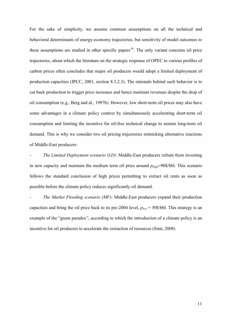
The carbon price follows a similar trajectory under the two oil pricing strategies, with three

distinct periods (Figure 3a).

Figure 3. (a) Carbon price ($/tCO2) [upper-left panel]; (b) Oil price ($/bbl) [upper-right panel]; (c) World Oil demand (Million b/d) [lower left panel]; (d) Total cost of a barrel of oil, including carbon costs ($/bbl) [lower-left panel]

During the first years of the climate policy (2010-2025), Middle-East producers have enough

leeway on the deployment of their production capacities to control oil prices, which are

therefore almost unaffected by the climate policy (Figure 3b). High carbon prices are

necessary to ensure a steady increase of the cost of oil for final users (Figure 3d) in turn

triggering the decrease of oil consumption necessary to comply with the reduction of carbon

emissions (Figure 3c). Under the MF scenario, the increase of carbon prices is sensibly

steeper (89$/tCO2 in 2025 vs. 70$/tCO2 under the LD scenario), but total oil demand remains

more important (105 Million b/d at the maximum vs. 97 Million b/d in the LD scenario)

because of lower total cost of a barrel.

13

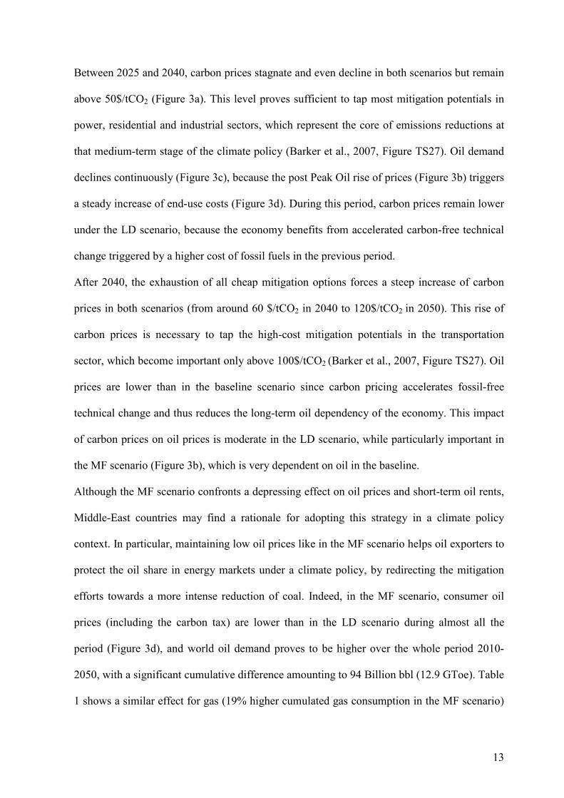
Between 2025 and 2040, carbon prices stagnate and even decline in both scenarios but remain

above 50$/tCO2 (Figure 3a). This level proves sufficient to tap most mitigation potentials in

power, residential and industrial sectors, which represent the core of emissions reductions at

that medium-term stage of the climate policy (Barker et al., 2007, Figure TS27). Oil demand

declines continuously (Figure 3c), because the post Peak Oil rise of prices (Figure 3b) triggers

a steady increase of end-use costs (Figure 3d). During this period, carbon prices remain lower

under the LD scenario, because the economy benefits from accelerated carbon-free technical

change triggered by a higher cost of fossil fuels in the previous period.

After 2040, the exhaustion of all cheap mitigation options forces a steep increase of carbon

prices in both scenarios (from around 60 $/tCO2 in 2040 to 120$/tCO2 in 2050). This rise of

carbon prices is necessary to tap the high-cost mitigation potentials in the transportation

sector, which become important only above 100$/tCO2 (Barker et al., 2007, Figure TS27). Oil

prices are lower than in the baseline scenario since carbon pricing accelerates fossil-free

technical change and thus reduces the long-term oil dependency of the economy. This impact

of carbon prices on oil prices is moderate in the LD scenario, while particularly important in

the MF scenario (Figure 3b), which is very dependent on oil in the baseline.

Although the MF scenario confronts a depressing effect on oil prices and short-term oil rents,

Middle-East countries may find a rationale for adopting this strategy in a climate policy

context. In particular, maintaining low oil prices like in the MF scenario helps oil exporters to

protect the oil share in energy markets under a climate policy, by redirecting the mitigation

efforts towards a more intense reduction of coal. Indeed, in the MF scenario, consumer oil

prices (including the carbon tax) are lower than in the LD scenario during almost all the

period (Figure 3d), and world oil demand proves to be higher over the whole period 2010-

2050, with a significant cumulative difference amounting to 94 Billion bbl (12.9 GToe). Table

1 shows a similar effect for gas (19% higher cumulated gas consumption in the MF scenario)

14

because of the indexation of gas prices on oil prices when they remain sufficiently low. Given

the identical climate objectives forcing identical carbon emissions in total the higher oil and

gas consumption under MF scenario must be offset by lower coal production (12% less

cumulative production over 2010-2050). Although the numerical differences are moderate in

terms of cumulated production, the next section will show that this will have significant

impacts on exportation revenues over the period.

Table 1. Cumulated production of fossil fuels under climate policy over the period 2010-2050 (GToe)

Oil Gas Coal

LD scenario 182.3 97 162.6

MF scenario 195.2 115.1 142.9

Relative difference (MF vs LD) + 7% + 19% - 12 %

2.2 The climate policy and Middle-East countries’ economy

Unsurprisingly, whatever the oil pricing strategy, the introduction of a carbon price induces a

significant drop of oil revenues in Middle-East countries (Figure 4). Note that this measure

compares the level of revenues reached in the two different baselines with that under climate

policy. This comes down to assuming that Middle-East’s choice between MF and LD is less

influenced by the climate policy than by the intrinsic time preference characterizing the trade-

off between short- and long-term effects.17

15

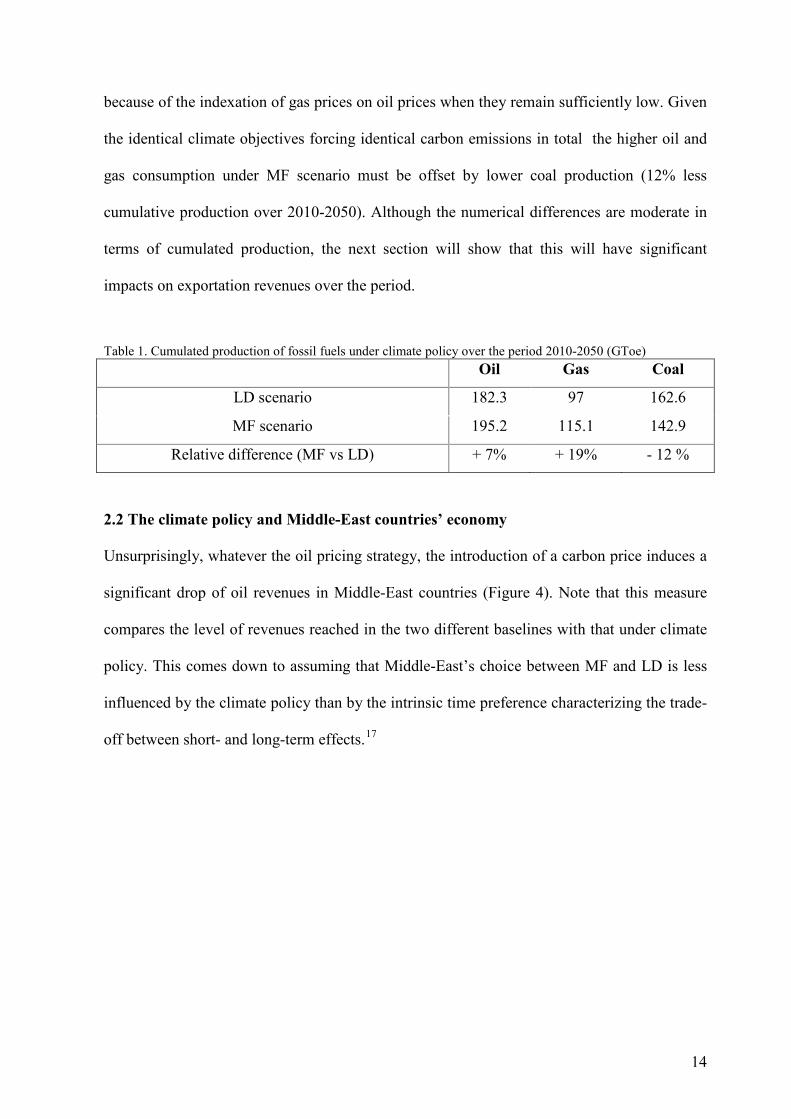
Figure 4. Reduction of oil exportation revenues under climate policy (Billion $)

In the short-term, as discussed in section 2.1, price levels are almost unaffected by the climate

policy and the reduction of oil exportation revenues is due to the drop of oil demand. In the

longer term, price effects enter into play and magnify the revenue losses, especially in the MF

scenario where costs reach $10 700 Billion over the whole period, or 26% of cumulated oil

revenues,. This is because the climate policy delays Peak Oil and minors its consequences in

terms of rising prices, hence strongly limiting the high long-term profits Middle-East

countries receive in the baseline case. This effect is also at play under the Low Deployment

scenario but with a lower magnitude so that cumulative losses are limited to $6 000 Billion

over 2010-2050, or 16% of total oil revenues.

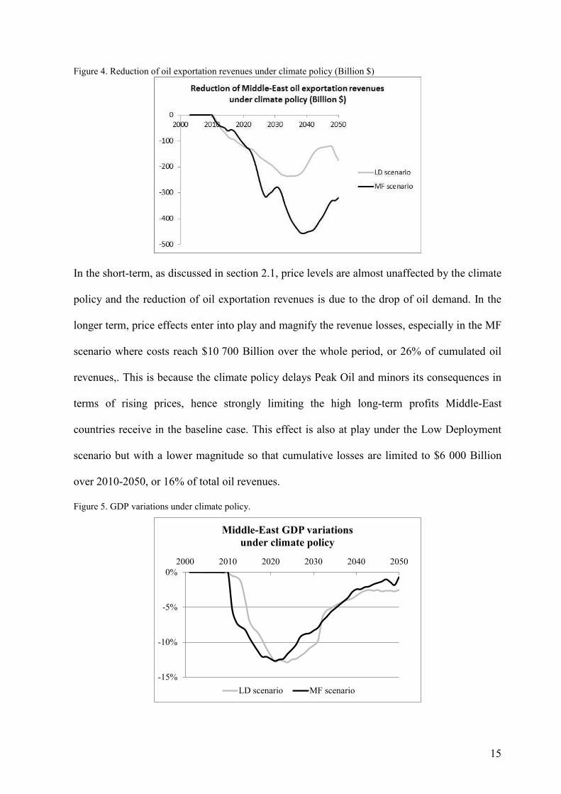
Figure 5. GDP variations under climate policy.

-15%

-10%

-5%

0%

2000 2010 2020 2030 2040 2050

Middle-East GDP variations

under climate policy

LD scenario MF scenario

16

Less intuitive is the somewhat different picture obtained by observing the macroeconomic

losses in Middle-East countries (Figure 5).

Over the short-term (2010-2020), the contraction of economic activity reaches a very

significant 12.5% losses, which corresponds to an average 1% reduction of growth rates over

2010-2020 (3.5% instead of 4.5%). This is due to the sharply upward-oriented carbon prices

at this time horizon and to inertias on the renewal of technologies and end-use equipment

which inhibit the capacity of producers and consumers to escape the increase of their energy

bill. These effects cause significant increases of production costs and final prices undermining

competitiveness of non-energy sectors and consumers’ purchase power. Those effects

combine to generate a drop in final demand, a contraction of production, higher

unemployment and an additional weakening of households’ purchase power. Although valid

for any region, these mechanisms are particularly important in Middle-East countries because

of the high fossil-intensity of production process driving high energy costs (especially when

compared with labour costs), and of the high share of energy expenditures in households’

budget.18

Over the long run, despite the permanent gap in oil revenues, macroeconomic activity

experiences a recovery phase and GDP levels in 2050 are very close to baseline levels (only

1% and 3% losses under MF and LD scenarios, respectively). This means that a drop of oil

revenues as experienced under a climate policy is not necessarily univocally penalizing for

economic activity. This can be analysed as the end of the ‘natural resource curse’ (Sachs and

Warner, 2001). In the present case of an exogenous assumption about the current account

balance, lower oil exportation revenues imply a lower exchange rate of local currencies

favoring the competitiveness of domestic industries. The climate policy then fosters local

production at the expense of industrial goods importation and induces a faster

industrialization in Middle-East countries which better prepares Middle-East’s economies to

17

the post oil era. Long-run economic activity is less sensitive to oil revenues and those

revenues fall into a more mature production structure apt to absorb them efficiently. This is

critically illustrated by the MF scenario, in which almost the same GDP levels are reached in

2050 despite 25% lower oil revenues at that time horizon.

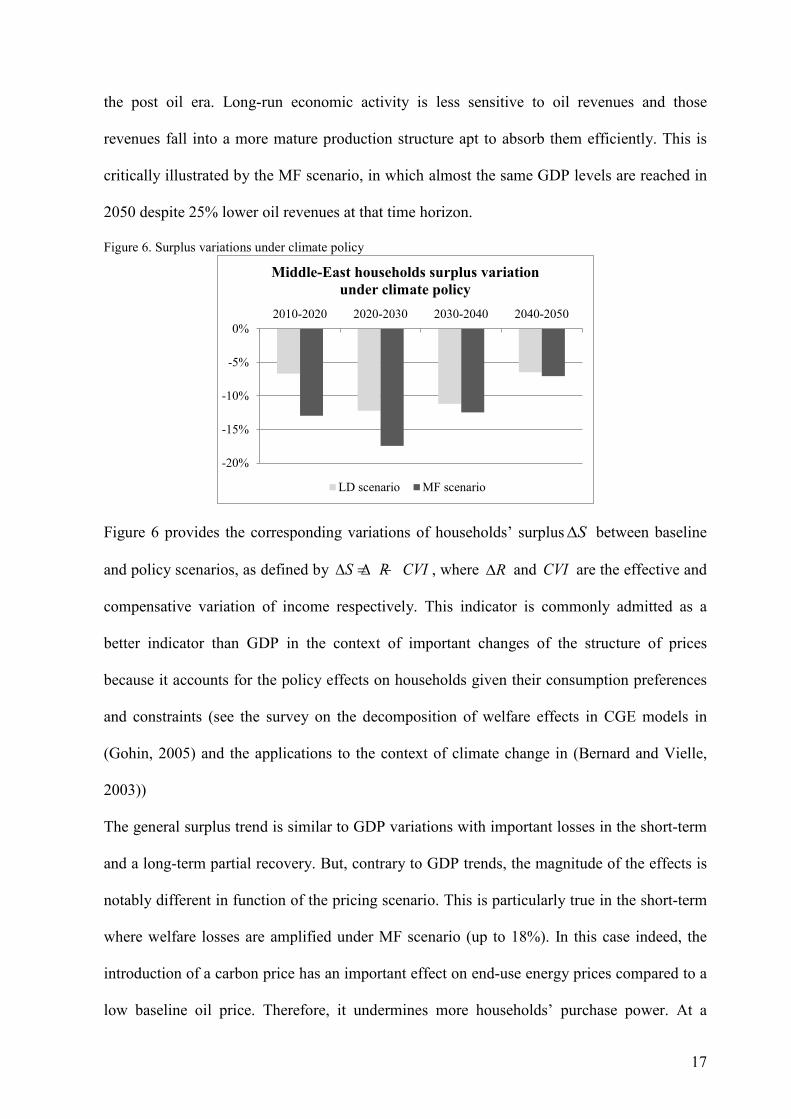
Figure 6. Surplus variations under climate policy

Figure 6 provides the corresponding variations of households’ surplus S∆ between baseline

and policy scenarios, as defined by S R CVI∆ = ∆ − , where R∆ and CVI are the effective and

compensative variation of income respectively. This indicator is commonly admitted as a

better indicator than GDP in the context of important changes of the structure of prices

because it accounts for the policy effects on households given their consumption preferences

and constraints (see the survey on the decomposition of welfare effects in CGE models in

(Gohin, 2005) and the applications to the context of climate change in (Bernard and Vielle,

2003))

The general surplus trend is similar to GDP variations with important losses in the short-term

and a long-term partial recovery. But, contrary to GDP trends, the magnitude of the effects is

notably different in function of the pricing scenario. This is particularly true in the short-term

where welfare losses are amplified under MF scenario (up to 18%). In this case indeed, the

introduction of a carbon price has an important effect on end-use energy prices compared to a

low baseline oil price. Therefore, it undermines more households’ purchase power. At a

-20%

-15%

-10%

-5%

0%

2010-2020 2020-2030 2030-2040 2040-2050

Middle-East households surplus variation

under climate policy

LD scenario MF scenario

18

longer term horizon, the recovery of surplus levels proves to be less important than the

recovery of GDP: surplus levels are still around 5% lower than in the baseline in 2050. Again,

the inertias limiting the changes of consumption patterns hamper the reduction of oil-intensity

for final demand. In particular, constrained mobility needs for daily travels (essentially,

commuting and shopping) force the consumption of fossil fuels without increasing welfare

levels.

3. Climate policy and Monetary Compensations (MC) for oil producers:

framing the debate.

The previous section has demonstrated that, although the costs of the climate policy are

significantly reduced when considering economic activity instead of oil revenues,

macroeconomic assessments still feature a risk of high costs in Middle-East economies,

especially in the transitory period. This assessment confirms the intuition that the international

community will have to think of complementary measures to limit the adverse impacts of

climate policies to gain the compliance of major oil-exporting economies. We consider now

the simplest of such measure, i.e. the implementation of Monetary Compensations (hereafter

denoted as MC) for which two rationales can be envisaged. Their amount and time-profile can

be calculated to compensate either the losses of oil exportation revenues (sectoral MC) or the

drop of economic activity (macroeconomic MC) (Figure 7).

19

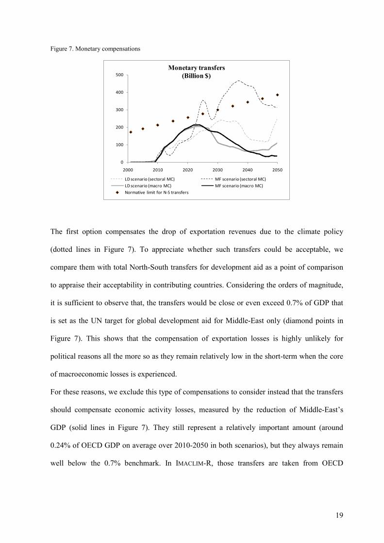
Figure 7. Monetary compensations

The first option compensates the drop of exportation revenues due to the climate policy

(dotted lines in Figure 7). To appreciate whether such transfers could be acceptable, we

compare them with total North-South transfers for development aid as a point of comparison

to appraise their acceptability in contributing countries. Considering the orders of magnitude,

it is sufficient to observe that, the transfers would be close or even exceed 0.7% of GDP that

is set as the UN target for global development aid for Middle-East only (diamond points in

Figure 7). This shows that the compensation of exportation losses is highly unlikely for

political reasons all the more so as they remain relatively low in the short-term when the core

of macroeconomic losses is experienced.

For these reasons, we exclude this type of compensations to consider instead that the transfers

should compensate economic activity losses, measured by the reduction of Middle-East’s

GDP (solid lines in Figure 7). They still represent a relatively important amount (around

0.24% of OECD GDP on average over 2010-2050 in both scenarios), but they always remain

well below the 0.7% benchmark. In IMACLIM-R, those transfers are taken from OECD

0

100

200

300

400

500

2000 2010 2020 2030 2040 2050

Monetary transfers

(Billion $)

LD scenario (sectoral MC) MF scenario (sectoral MC)

LD scenario (macro MC) MF scenario (macro MC)

Normative limit for N-S transfers

20

countries’ state budget in proportion of each country’s share in total OECD GDP, and are

given to Middle-Eastern in the form of capital flows.

The next sections assess the efficiency of such forms of compensations in their purpose to

sustain Middle-East economy. They do so by investigating, analytically in section 4 and

quantitatively in section 5, the mechanisms at play and the consequences of their

implementation when a general equilibrium perspective is adopted.

4. The macroeconomy of monetary transfers. An analytical detour

Under a partial equilibrium framework, the additional revenue coming from monetary

compensations would directly translate into an identical increase of domestic economic

activity. But, when general equilibrium interactions are taken into account, the impact of

monetary compensations becomes less straightforward because of their feedback effect on the

terms-of-trade, which causes adjustments on international markets affecting domestic

production and labour markets.

This section proposes an analytical framework to isolate the general equilibrium effects of

monetary transfers when these three dimensions of interaction are taken into account. The

specifications used hereafter in equations (1), (2) and (3) are similar to the ones adopted in the

IMACLIM-R for the representation of goods supply, labour markets and international trade (as

described by equations (SM-7), (SM-10), (SM-19)-(SM-22) respectively in the

Supplementary Material of (Waisman et al, 2012a)).

4.1 Model specifications

We consider an energy-exporting economy, which produces a composite good Q sold at price

p and energy E sold at price pE.

21

The composite good is produced with energy and labour as production factors. Unitary energy

and labour requirements for production are defined by e and l, respectively, the wage rate is

noted w and a mark-up rate π over production costs captures imperfect competition. The price

level is then given by

. . .Ep e p w l pπ= + + (1)

Labour markets are described by a wage curve introducing an inverse relationship between

the wage rate and unemployment.19 This means that the real wage level is an increasing

function of the number of employed workers L lQ= :

wwL

p

α= (2)

Here, w is a constant and 0α > is the elasticity of the wage curve: the higher α , the more

flexible the labour markets.

Finally, the trade balance for the composite good is an increasing function of the price

differential between local prices p and world price pw: the higher the local production price

(relatively to international levels), the more agents have incentives to rely on imported goods

M and to reduce exportations X. For the sake of simplicity; we assume a simplified

dependence between the trade balance wp M pX− and relative pricesw

p

p:

w

w

pp M pX I

p

β − = (3)

Here I is a constant and 0β > is the elasticity of the trade balance to price differentials: the

higher β the more the trade balance is sensitive to price variations.

Setting the world price as the numéraire (pw=1), the equilibrium of the balance of payments

gives:

w E Ep M K pX p X T+ = + + (4)

22

Here, K measures (relative) capital exportations and T represents the transfers received for

compensation of the adverse impacts of the climate policy.

4.2 Results and interpretation

Capital export K is exogenously set (see discussion in section 1.3), and is therefore

independent from the level of monetary transfers. Given the small size of transfers with

respect to total income in oil-consuming countries (around 0.24% of OECD), we make the

additional assumption that energy demand is not altered and hence that energy variables pE

and XE are not affected by the introduction of monetary transfers.

By noting p0 and Q0 the price and production levels in absence of monetary compensations,

the Laspeyres index of economic activity, which measures GDP levels in quantity units after

the introduction of monetary transfers, is defined by:

0E EGDP p X p Q= + (5)

We introduce the “efficiency index of monetary transfers”,Tη , as the ratio of GDP variations

due to monetary compensation over the amount of transfers:

0T

GDP GDP

Tη −= (6)

A value Tη means that 1$ in monetary compensation brings Tη $ of economic activity. Cases

where 1Tη > mean that monetary transfer have a more than proportional stimulating effect on

economic activity, whereas on the contrary 1Tη < mean that general equilibrium interactions

trigger a negative feedback effect limiting the stimulation of economic activity.

A direct calculation (see Appendix) gives

( )1

1T

v

v u

εη αβ−≈ − (7)

23

Here, three parameters characterizing the domestic economy (in terms of production

structures and exposure to international competition) prove to play a crucial role:

• 0

Ep e

w lε = the ratio of energy costs to labour costs in production processes

• 0

E Ep Xv

GDP= the dependence of the local economy on energy exportations.

• E E

Ku

p X= the relative importance of capital exports to energy exports.

The effect of monetary transfers on ex-post economic activity is stronger, as captured by

higher Tη , when (i) labor market rigidities are important (low α ) and production processes

are energy-intensive (highε ). Under the assumption of equilibrated balance of payments, the

transfers must be compensated by additional exports and hence a gain of competitiveness.

Rigid labor markets mean that these adjustments do not affect significantly real wages and

hence households’ purchase power, but rather rely on international effects on terms-of-trade.

This is even truer in economies where labor represents a moderate share of production costs

so that the efforts towards more competitive production processes affects through non-labor

inputs; (ii) domestic sectors are less exposed to international trade, as captured by less intense

competition on industrial goods (low β ), less dependence on energy exportation revenues

(low v ) and high capital exports (high u). In this case indeed, monetary transfers play a

minored role in the position of the local economy on international markets.

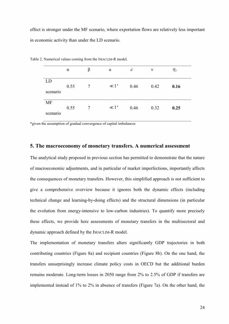
Table 2 provides numerical assessments of Tη when considering numerical values adopted in

the IMACLIM-R model. Two general comments can be derived from this quantification. First,

the efficiency of monetary transfers is far lower than one, which means that general

equilibrium interactions under market imperfections (on labour markets, international trade

and industrial production) limit the positive stimulus given by monetary transfers. Second, the

24

effect is stronger under the MF scenario, where exportation flows are relatively less important

in economic activity than under the LD scenario.

Table 2. Numerical values coming from the IMACLIM-R model.

α β u ε ν Tη

LD

scenario 0.55 7 1 * 0.46 0.42 0.16

MF

scenario 0.55 7 1 * 0.46 0.32 0.25

*given the assumption of gradual convergence of capital imbalances

5. The macroeconomy of monetary transfers. A numerical assessment

The analytical study proposed in previous section has permitted to demonstrate that the nature

of macroeconomic adjustments, and in particular of market imperfections, importantly affects

the consequences of monetary transfers. However, this simplified approach is not sufficient to

give a comprehensive overview because it ignores both the dynamic effects (including

technical change and learning-by-doing effects) and the structural dimensions (in particular

the evolution from energy-intensive to low-carbon industries). To quantify more precisely

these effects, we provide here assessments of monetary transfers in the multisectoral and

dynamic approach defined by the IMACLIM-R model.

The implementation of monetary transfers alters significantly GDP trajectories in both

contributing countries (Figure 8a) and recipient countries (Figure 8b). On the one hand, the

transfers unsurprisingly increase climate policy costs in OECD but the additional burden

remains moderate. Long-term losses in 2050 range from 2% to 2.5% of GDP if transfers are

implemented instead of 1% to 2% in absence of transfers (Figure 7a). On the other hand, the

25

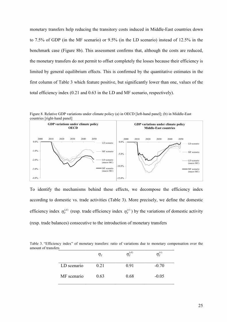
monetary transfers help reducing the transitory costs induced in Middle-East countries down

to 7.5% of GDP (in the MF scenario) or 9.5% (in the LD scenario) instead of 12.5% in the

benchmark case (Figure 8b). This assessment confirms that, although the costs are reduced,

the monetary transfers do not permit to offset completely the losses because their efficiency is

limited by general equilibrium effects. This is confirmed by the quantitative estimates in the

first column of Table 3 which feature positive, but significantly lower than one, values of the

total efficiency index (0.21 and 0.63 in the LD and MF scenario, respectively).

Figure 8. Relative GDP variations under climate policy (a) in OECD [left-hand panel]; (b) in Middle-East countries [right-hand panel]

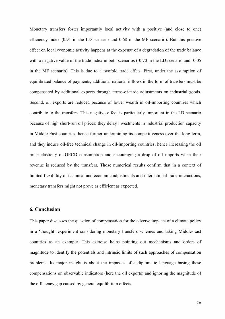
To identify the mechanisms behind these effects, we decompose the efficiency index

according to domestic vs. trade activities (Table 3). More precisely, we define the domestic

efficiency index ( )d

Tη (resp. trade efficiency index ( )t

Tη ) by the variations of domestic activity

(resp. trade balances) consecutive to the introduction of monetary transfers

Table 3. “Efficiency index” of monetary transfers: ratio of variations due to monetary compensation over the amount of transfers

Tη ( )d

Tη ( )t

Tη

LD scenario 0.21 0.91 -0.70

MF scenario 0.63 0.68 -0.05

-4.0%

-3.0%

-2.0%

-1.0%

0.0%

2000 2010 2020 2030 2040 2050

GDP variations under climate policy

OECD

LD scenario

MF scenario

LD scenario(macro MC)

MF scenario(macro MC)

-15.0%

-10.0%

-5.0%

0.0%

2000 2010 2020 2030 2040 2050

GDP variations under climate policy

Middle-East countries

LD scenario

MF scenario

LD scenario(macro MC)

MF scenario(macro MC)

26

Monetary transfers foster importantly local activity with a positive (and close to one)

efficiency index (0.91 in the LD scenario and 0.68 in the MF scenario). But this positive

effect on local economic activity happens at the expense of a degradation of the trade balance

with a negative value of the trade index in both scenarios (-0.70 in the LD scenario and -0.05

in the MF scenario). This is due to a twofold trade effets. First, under the assumption of

equilibrated balance of payments, additional national inflows in the form of transfers must be

compensated by additional exports through terms-of-tarde adjustments on industrial goods.

Second, oil exports are reduced because of lower wealth in oil-importing countries which

contribute to the transfers. This negative effect is particularly important in the LD scenario

because of high short-run oil prices: they delay investments in industrial production capacity

in Middle-East countries, hence further undermining its competitiveness over the long term,

and they induce oil-free technical change in oil-importing countries, hence increasing the oil

price elasticity of OECD consumption and encouraging a drop of oil imports when their

revenue is reduced by the transfers. Those numerical results confirm that in a context of

limited flexibility of technical and economic adjustments and international trade interactions,

monetary transfers might not prove as efficient as expected.

6. Conclusion

This paper discusses the question of compensation for the adverse impacts of a climate policy

in a ‘thought’ experiment considering monetary transfers schemes and taking Middle-East

countries as an example. This exercise helps pointing out mechanisms and orders of

magnitude to identify the potentials and intrinsic limits of such approaches of compensation

problems. Its major insight is about the impasses of a diplomatic language basing these

compensations on observable indicators (here the oil exports) and ignoring the magnitude of

the efficiency gap caused by general equilibrium effects.

27

In a general equilibrium model representing the interactions between oil markets and the

macroeconomy, we first show a time-lag between losses of oil exports and of macroeconomic

activity measured in GDP. Oil export losses remain moderate in the short term, especially

under a ‘low deployment strategy’ of oil production, while the GDP losses can be very high

because Middle-East countries cannot quickly adjust to very high increase of their (currently

very low) domestic energy prices. This mismatch explains why compensating transfers based

on oil revenue losses cannot solve the transition problem.

But, even fine-tuning compensations according to GDP losses proves to compensate only

partly the economic slowdown due to a carbon constraint because of general equilibrium

feedbacks which undermine the macroeconomic efficiency of monetary transfers. This

‘efficiency gap’ of transfers results in particular from the dependence of the domestic output

to oil exportation revenues, the sensitivity of non energy sectors to price competition and the

labour market rigidities which restrict the adaptive capacity of economies to changing

conditions.

In addition to this intrinsic limit to the effectiveness of transfers, our results show that the

magnitude of the GDP losses to be compensated cannot rely on observable parameters since

the magnitude of the efficiency gap of transfers is determined by the strategic choices of the

Middle-East and also by the capacity of domestic policies to block Dutch disease

mechanisms.

These results show, beyond the specific case of oil exporters, the trap of reducing the

compensation problem in climate negotiations to a question of monetary transfers. Other

options are to be envisaged like technological transfers (Barrett, 2001, 2003) or innovative

devices in climate finance (Hourcade et al. 2012) to ease the structural transition towards low

carbon development paths and, in the case of Middle-East countries, towards the “beyond oil”

era.

28

Acknowledgments:

Special thanks to participants of the SURED 2012 conference for helpful comments and

suggestions. The authors acknowledge funding by the Chair “Modeling for sustainable

development” (led by Mines ParisTech, Ecole des PontsParisTech, AgroParisTech and

ParisTech) and the EU FP-7 projects GLOBIS and AUGUR.

29

REFERENCES

Apergis, N, Tsoumas, C, 2009. A survey of the Feldstein_Horioka puzzle: What has been done and where we

stand. Research in Economics 63, 64-76.

Armington, P, 1969. A Theory of Demand for Products Distinguished by Place of Production. IMF,

International Monetary Fund Staff Papers 16, 170-201.

Atkeson, A., Kehoe, P.J., 1999. Models of energy use: putty-putty versus putty-clay. The American Economic

Review, 89(4), 1028-1043.

Barker T, Bashmakov I, Bernstein L, Bogner JE, Bosch PR, Dave R, Davidson OR, Fisher BS, Gupta S, Halsnæs

K, Heij GJ, Kahn Ribeiro S, Kobayashi S, Levine MD, Martino DL, Masera O, Metz B, Meyer LA,

Nabuurs G-J, Najam A, Nakicenovic N, Rogner HH, Roy J, Sathaye J, Schock R, Shukla P, Sims REH,

Smith P, Tirpak DA, Urge-Vorsatz D, Zhou D (2007): Technical Summary. In: Climate Change 2007:

Mitigation. Contribution of Working Group III to the Fourth Assessment Report of the Intergovernmental

Panel on Climate Change [B. Metz, O. R. Davidson, P. R. Bosch, R. Dave, L. A. Meyer (eds)],

Cambridge University Press, Cambridge, United Kingdom and New York, NY, USA.

Barnett, J, Dessai, S, Webber M, 2004. Will OPEC lose from the Kyoto Protocol? Energy Policy, 32(18), 2077-

2088.

Barnett, J, Dessai, S, 2002. Articles 4.8 and 4.9 of the UNFCCC: adverse effects and the impacts of response

measures. Climate Policy 2(2-3), 231-239.

Barrett, S, 2003. Environment and Statecraft: the Strategy of Environmental Treaty-Making.Oxford University

Press.

Barrett, S, 2001. Towards a Better Treaty. Policy Matters 01-29, Washington, DC: AEI Brookings Joint Center

for Regulatory Studies.

Berg, E, Kverndokk, S, Rosendahl, K, 1997a. Gains from cartelisation in the oil market. Energy Policy 25 (13),

1075-1091.

Berg, E, Kverndokk, S, Rosendahl K, 1997b. Market Power, International CO2 Taxation and Petroleum Wealth

.The Energy Journal 18(4), 33-71.

Bernard, A, Vielle, M, 2003. Measuring the welfare cost of climate change policies: A comparative assessment

based on the computable general equilibrium model GEMINI-E3. Environmental Modeling and

Assessment 8,199–217.

30

Blanchflower, DG, Oswald, AJ, 1995. An introduction to the wage curve.The Journal of Economic Perspectives:

153-167.

Boone, P, 1996. Politics and the effectiveness of foreign aid. European Economic Review 40(2), 289–329.

Bresnahan, T.F., Ramey, V.A., 1993. Segment Shifts and Capacity Utilization in the U.S. Automobile Industry.

American Economic Review Papers and Proceedings, 83(2), 213-218.

Burnside, C., Dollar, D., 2000. Aid, policies and growth. American Economic Review90(4), 847–869.

Collier, P., Dollar, D., 2001. Can the world cut poverty in half? How policy reformand effective aid can meet

international development goals. World Development29(11), 1787–1802.

Dalgaard, C.-J., Hansen, H., Tarp, F., 2004. On the empirics of foreign aid andgrowth. Economic Journal

114(496), 191–216.

Davis, S., Haltiwanger, J.,2001. Sectoral Job Creation and Destruction Responses to Oil Price Changes. Journal

of Monetary Economics, 48, 465-512.

Doucouliagos, H., Paldam, M, 2011. The ineffectiveness of development aid on growth : An update. European

Journal of Political Economy 27, 399-404.

Easterly, W, 2005. What did structural adjustment adjust? The association of policiesand growth with repeated

IMF and World Bank adjustment loans.Journalof Development Economics, 76(1), 1–22.

Easterly, W, Levine, R., Roodman, D., 2004. New data, new doubts: A comment on burnside and dollar’s “Aid,

Policies and Growth”. Center for Global Development Working Paper No. 26, Washington, D.C.

Feldstein, M, Horioka, C, 1980. Domestic savings and international capital flows. The Economic Journal 90,

314-329.

Finn, MG, 2000. Perfect competition and the effects of energy price increases on economic activity.

Journal of Money, Credit and Banking, 32(3), 400-416.

Frankel, J.A., 2010. The Natural Resource Curse: A Survey. NBER Working Paper No. 15836

Gohin, A, 2005. The specification of price and income elasticities in computable general equilibrium models: An

application of latent separability. Economic Modelling 22(5), 905-925

Guillaumont, P., Chauvet, L., 2001. Aid and performance: A reassessment. JournalofDevelopmentStudies, 37(6),

66–92.

Guivarch, C., Crassous, R., Sassi, O., Hallegatte, S., 2011. The costs of climate policies in a second best world

with labour market imperfections. Climate Policy 11, 768–788.

Hamilton, J.D., 2008. Oil and the Macroeconomy.The New Palgrave Dictionary of Economics.

31

Hogendorn, C, 1998. Capital Mobility in Historical Perspective Journal of Policy Modeling 20(2):141–161

(1998)

Hourcade JC, Perrissin-Fabert, B, Rozenberg J., 2012. Venturing into uncharted financial waters: an essayon

climate-friendly finance. International Environmental Agreements 12,165–186.

Hourcade JC, Jaccard M, Bataille C, Ghersi F, 2006. Hybrid Modeling : New Answers to Old Challenges. In:

Hybrid Modeling of Energy-Environment Policies: reconciling Bottom-up and Top-down. The Energy

Journal (Special Issue 2): 1-12.

Intergovernmental Panel on Climate Change (IPCC), 2001. Climate Change (2001): The Scientific Basis.

Cambridge University Press, Cambridge.

Johansen L, 1959. Substitution versus Fixed Production Coefficients in the Theory of Growth: A synthesis.

Econometrica 27, 157-176.

Johansson, D, Azar, C, Lindgren, K, Persson, T, 2009. OPEC Strategies and Oil Rent in a Climate Conscious

World. The Energy Journal 30 (3), 23-50.

Layard, R., Nickell, S., Jackman, R., 2005.Unemployment. Oxford University Press, Oxford.

Layard, R., Nickell,S., 1986.Unemployment in Britain.Economica 53, no. 210. New Series: S121-S169.

Luderer, G, DeCian, E, Hourcade, JC, Leimbach, M, Waisman, H, Edenhofer, O (2012). On the regional

distribution of mitigation costs in a global cap-and-trade regime. Climatic Change 114 (1): 59-78.

McKibbin, W.J., Ross, M.T., Shackleton, R., Wilcoxen, P.J., 1999. Emissions trading, capital flows and the

Kyoto Protocol. In: Weyant, J. (Ed.), TheCosts of the Kyoto Protocol: A Multi-Model Evaluation, Energy

Journal, Special Issue, pp. 287–333

Minoiu C, Reddy S., 2010. Development aid and economic growth: a positive long-run relation. The Quarterly

Review of Economics and Finance 50, 27-39.

Persson T, Azar C, Johansson D, Lindgren K, 2007. Major oil exporters may profit rather than lose, in a carbon-

constrained world. Energy Policy 35(12), 6346-6353.

Phelps, E., 1961. The Golden Rule of Accumulation: A Fable for Growthmen. The American Economic Review

51(4), 638-643

Rajan, R., Subramanian, A., 2011.Aid, Dutch disease, and manufacturing growth.Journal of Development

Economics94 (1): 106–118

Rajan, R., Subramanian, A., 2005. What undermines aid’s impact on growth?National Bureau of Economic

Research Working Paper No. 11657, Cambridge,MA.

32

Rehrl T, Friedrich, R, 2006.Modeling long-term oil price and extraction with a Hubbert approach: The LOPEX

model. Energy Policy 34(15):2413-2428.

Ross, M, 2012. The Oil Curse: How Petroleum Wealth Shapes the Development of Nations. Princeton

University Press

Rotemberg, J., Woodford, M., 1996. Imperfect Competition and theEffects of Energy Price Increases. Journal of

Money, Credit, and Banking, 28, 549-577.

Rozenberg, J., Hallegatte, S., Vogt-Schilb, A., Sassi, O., Guivarch, C., Waisman, H.,Hourcade, J-C., 2010.

Climate policies as a hedge against the uncertainty on future oil supply. Climatic Change,101(3-4),

663-668

Sachs, J.D., Warner, A.M., 2001. The Curse of Natural Resources. European Economic Review 45(4–6), 827–

838.

Sands RD, Miller S, Kim MK, 2005. The Second Generation Model: Comparison of SGM and GTAP

Approaches to Data Development, Pacific Northwest National Labouratory, PNNL-15467, 2005.

Saunders, H.D., 2013. Historical evidence for energy consumption rebound in 30 US sectors and a toolkit for

rebound analysts. Technological Forecasting and Social Change (in press).

http://dx.doi.org/10.1016/j.techfore.2012.12.007 .

Saunders, H.D., 2008. Fuel conserving (and using) production functions, Energy Economics 30, 2184 2235.

Shapiro, C.,.StiglitzJ E., 1984. Equilibrium Unemployment as a Worker Discipline Device.The American

Economic Review 74, no. 3: 433-444.

Sinn, H.W., 2008. Public policies against global warming. International Tax and Public Finance, 15(4), 360-394.

Tavoni M, DeCian E, Luderer G, Steckel JC, Waisman H (2012). The value of technology and of its evolution

towards a low carbon economy, Climatic Change 114 (1), 39-57.

van Vuuren DP, den Elzen MGJ, Berk MM, Lucas P, Eickhout B, Eerens H, Oostenrijk R, 2003. Regional costs

and benefits of alternative post-Kyoto climate regimes: comparison of variants of the multi-stage and per

capita convergence regime. Report 728001025, RIVM, Bilthoven, the Netherlands.

Waisman, H, Guivarch, C, Grazi, F., Hourcade, JC(2012a). The Imaclim-R Model: Infrastructures, Technical

Inertia and the Costs of Low Carbon Futures under Imperfect Foresight. Climatic Change 114 (1), 101-

120.

Waisman H., J. Rozenberg, O. Sassi, J.-C.Hourcade (2012b). Peak Oil profiles through the lens of a general

equilibrium assessment, Energy Policy 48, 744-753.

33

WBGU (2003). Climate Protection Strategies for the 21st Century: Kyoto and Beyond. German Advisory

Council on Global Change, Berlin, Germany.

ENDNOTES

1 It commits parties to give: “full consideration to [...] to the specific needs and concerns of developing country

parties arising from the adverse effects of climate change and/or the impact of the implementation of response

measures, especially on [...] countries whose economies are highly dependent on income generated from the

production, processing and export of fossil fuels and associated energy-intensiveproducts”.

2 It requires developed countries to implement their Kyoto commitments “in such a way so as to minimize

adverse social, environmental and economic impacts on developing country parties”, particularly those

identifiedin Articles 4.8 and 4.9 of the Convention.

3, which recognizes “the potential impacts of response measures on countries particularly vulnerable to its

adverse effects”.

4 In a survey of modeling exercises, (Barnett et al., 2004) estimate that the implementation of the Kyoto Protocol

would reduce oil exportation revenues by 9.8% to 13%, and decrease real income by up to 3% in 2010. At a

longer term horizon, (Van Vuuren et al., 2003) estimate that a 550ppm target would induce a 35% decrease of oil

revenues in OPEC countries in 2050 and (WBGU, 2003) obtains that the total abatement cost can reach

approximately 2 per cent of GDP in Middle East at the same horizon.

5 Some studies even obtain that a climate policy can be beneficial to the producers of conventional oil by

affecting more the cost of their substitutes (unconventional oil, coal) (Persson et al., 2007) or by fostering an

increase of conventional oil rents in OPEC if they can exert their market power (Johansson et al, 2009).

6 See, among others, (Burnside & Dollar,2000; Guillaumont and Chauvet, 2001; Collier and Dollar, 2002;

Dalgaard et al, 2004; Minoiu and Reddy, 2010)

34

7 e.g., (Boone, 1996; Easterly et al., 2004; Easterly, 2005)

8 The IMACLIM-R model has been used in several publications about oil markets (Rozenberg et al., 2010;

Waisman et al, 2012b) and the comprehensive description of its analytical structure and numerical assumptions

is given in (Waisman et al., 2012a)

9 For an extensive discussion about production/cost functions in the energy field, see (Saunders, 2008)

10 This iteration between the technical and production dimensions of the economy is a way to address the

technical challenge to energy economists, raised by (Saunders, 2013), that is to “include measured, flexible

cost/production functions […] and use measured technology gains for all factors of production”.

11 The persistence of this market power under climate policy is conditional upon the ability of OPEC countries to

elaborate coordinated strategies despite intra-cartel tensions caused by the lowering of oil revenues. In line with

(Berg et al, 1997a) who show that gains from cartelization are hardly impacted by global carbon taxes, we admit

that the climate policy will not affect the cartel discipline.

12 For example, in a historical study of capital flows over the long term (1865-1992), (Hogendorn, 1998)

demonstrates that no simple rule emerges for capital flows dynamics, given the fluctuations of capital mobility

over time in parallel with different phases of international monetary and financial governance: high capital

mobility during the gold standard period (1880-1913), almost closed economies during the Interwar and Bretton

Woods periods (1914-1969) and increasing mobility in the modern period (1970-1992).

13 The issue of capital mobility has given rise to a large controversy since the econometric study by (Feldstein

and Horioka, 1980), who demonstrated low capital mobility over 1960-1974, in contradiction with widely shared

ideas. This ‘puzzle’ was the starting point of a large body of literature trying to identify the major drivers of

capital flows, but which has failed to reach consensual answers (see (Apergis and Tsoumas, 2009) for a survey).

14 We do not consider the case where Middle-East countries withdraw from the climate policy, since this would

make the debate on monetary compensations, at the core of the present study, irrelevant.

15 (Luderer et al, 2012) analyses the effect of alternative regional distribution of emission allowances on climate

policy costs.

16 eg, (Waisman et al, 2012a) on the role of technical, resource and behavioral assumptions; (Tavoni et al, 2012)

on the sensitivity to the availability of certain technologies (Nuclear, CCS, renewable); or (Guivarch et al, 2011)

on the role of labor market rigidities.

35

17 (Waisman et al, 2012b) obtains for example that, in absence of climate policy, Middle-East producers would

prefer the MF scenario only if their discount rate is lower than 6%.

18 Note that this effect is measured under the assumption that Middle-East governments maintain the current

levels of energy subsidies but do not seek to increase it to offset the increase of fuel prices due to the climate

policy because it would involve a non-affordable amount for public spending

19 Microeconometric evidence for such formulation was given in a seminal contribution by (Blanchflower and

Oswald 1995) and extensive theories have been developed to support such representation of the labour market

(see (Layard et al., 2005) for an overview). The basic idea is that high unemployment represents an outside threat

that leads workers to accept lower wages as from either the bargaining approach (Layard and Nickell, 1986) or

the wage-efficiency approach (Shapiro and Stiglitz, 1984).

Appendix: analytical resolution of model in Section 4

To simplify notations, we introduce:

• E E

Tx

p X= the ratio of monetary transfers over total energy exportation revenues, which

measures the magnitude of monetary transfers.

• 0

E Ep Xv

GDP= the dependence of the local economy on energy exportations.

• E E

Ku

p X= the relative importance of capital exports to energy exports.

• 0

Ep e

w lε = the ratio of energy costs to labour costs in production processes.

36

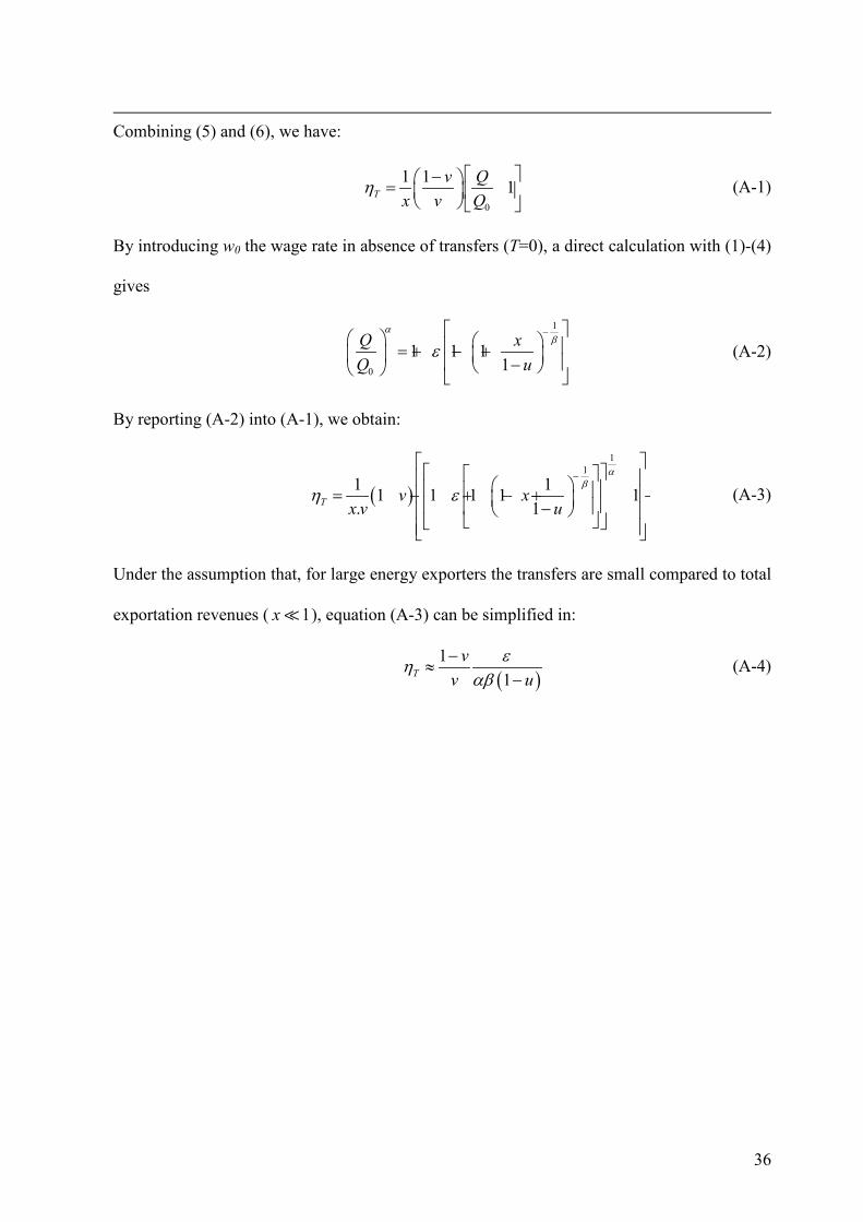
Combining (5) and (6), we have:

0

1 11T

v Q

x v Qη − = − (A-1)

By introducing w0 the wage rate in absence of transfers (T=0), a direct calculation with (1)-(4)

gives

1

0

1 1 11

Q x

Q u

α βε − = + − + − (A-2)

By reporting (A-2) into (A-1), we obtain:

( )1

1

1 11 1 1 1 1

. 1T v x

x v u

αβη ε − = − + − + − − (A-3)

Under the assumption that, for large energy exporters the transfers are small compared to total

exportation revenues ( 1x ), equation (A-3) can be simplified in:

( )1

1T

v

v u

εη αβ−≈ − (A-4)