Monetary EconomicsBasic Flexible Price Models

Nicola Viegi

July 26, 2017

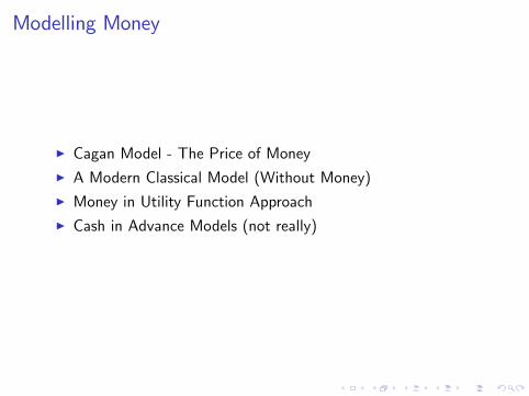
Modelling Money

I Cagan Model - The Price of MoneyI A Modern Classical Model (Without Money)I Money in Utility Function ApproachI Cash in Advance Models (not really)

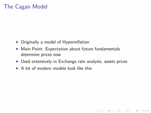
The Cagan Model

I Originally a model of Hyperin�ationI Main Point: Expectation about future fundamentalsdetermine prices now

I Used extensively in Exchange rate analysis, assets pricesI A lot of modern models look like this

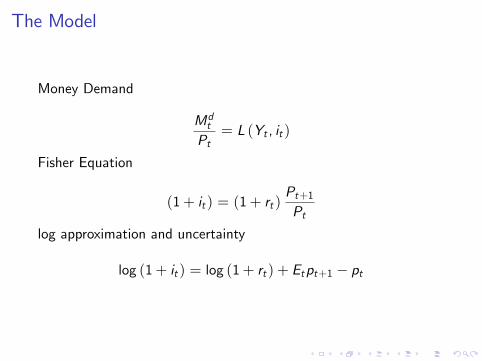
The Model

Money Demand

Mdt

Pt= L (Yt , it )

Fisher Equation

(1+ it ) = (1+ rt )Pt+1Pt

log approximation and uncertainty

log (1+ it ) = log (1+ rt ) + Etpt+1 � pt

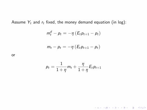
Assume Yt and rt �xed, the money demand equation (in log):

mdt � pt = �η (Etpt+1 � pt )

mt � pt = �η (Etpt+1 � pt )or

pt =1

1+ ηmt +

η

1+ ηEtpt+1

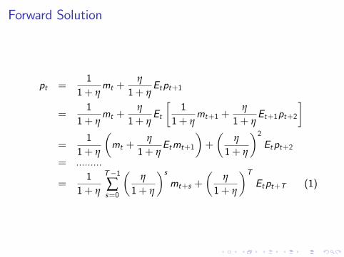
Forward Solution

pt =1

1+ ηmt +

η

1+ ηEtpt+1

=1

1+ ηmt +

η

1+ ηEt

�1

1+ ηmt+1 +

η

1+ ηEt+1pt+2

�=

11+ η

�mt +

η

1+ ηEtmt+1

�+

�η

1+ η

�2Etpt+2

= .........

=1

1+ η

T�1∑s=0

�η

1+ η

�smt+s +

�η

1+ η

�TEtpt+T (1)

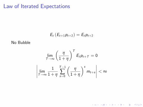
Law of Iterated Expectations

Et (Et+1pt+2) = Etpt+2

No Bubble

limT!∞

�η

1+ η

�TEtpt+T = 0����� limT!∞

11+ η

T�1∑s=0

�η

1+ η

�smt+s

����� < ∞

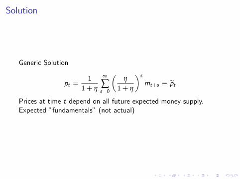
Solution

Generic Solution

pt =1

1+ η

∞

∑s=0

�η

1+ η

�smt+s � ept

Prices at time t depend on all future expected money supply.Expected �fundamentals� (not actual)

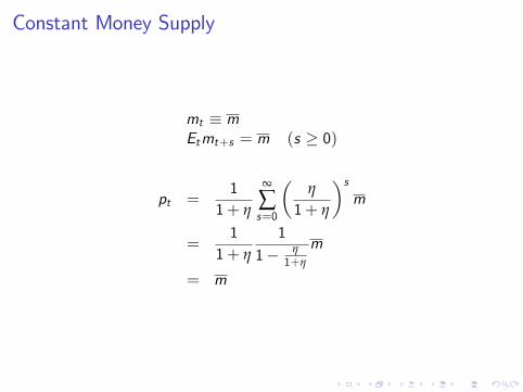
Constant Money Supply

mt � mEtmt+s = m (s � 0)

pt =1

1+ η

∞

∑s=0

�η

1+ η

�sm

=1

1+ η

11� η

1+η

m

= m

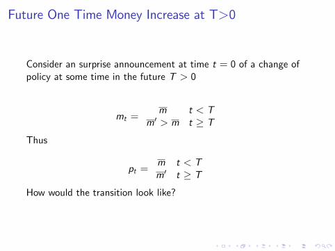
Future One Time Money Increase at T>0

Consider an surprise announcement at time t = 0 of a change ofpolicy at some time in the future T > 0

mt =m t < T

m0 > m t � TThus

pt =m t < Tm0 t � T

How would the transition look like?

Solution

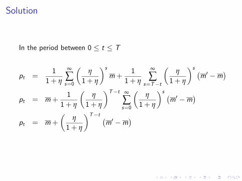
In the period between 0 � t � T

pt =1

1+ η

∞

∑s=0

�η

1+ η

�sm+

11+ η

∞

∑s=T�t

�η

1+ η

�s �m0 �m

�pt = m+

11+ η

�η

1+ η

�T�t ∞

∑s=0

�η

1+ η

�s �m0 �m

�pt = m+

�η

1+ η

�T�t �m0 �m

�

Solution

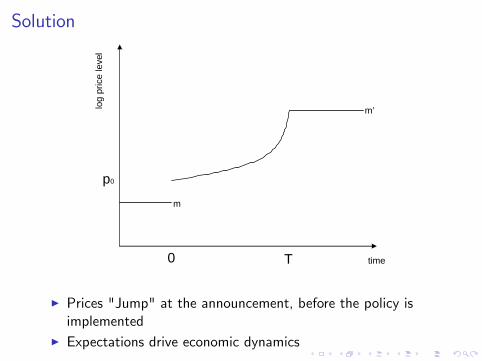
p0

0 T time

log

pric

e le

vel

m

m’

I Prices "Jump" at the announcement, before the policy isimplemented

I Expectations drive economic dynamics

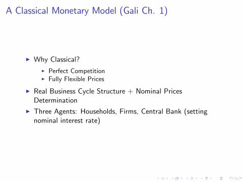
A Classical Monetary Model (Gali Ch. 1)

I Why Classical?I Perfect CompetitionI Fully Flexible Prices

I Real Business Cycle Structure + Nominal PricesDetermination

I Three Agents: Households, Firms, Central Bank (settingnominal interest rate)

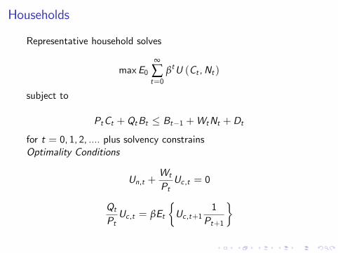
Households

Representative household solves

maxE0∞

∑t=0

βtU (Ct ,Nt )

subject to

PtCt +QtBt � Bt�1 +WtNt +Dt

for t = 0, 1, 2, .... plus solvency constrainsOptimality Conditions

Un,t +Wt

PtUc ,t = 0

QtPtUc ,t = βEt

�Uc ,t+1

1Pt+1

�

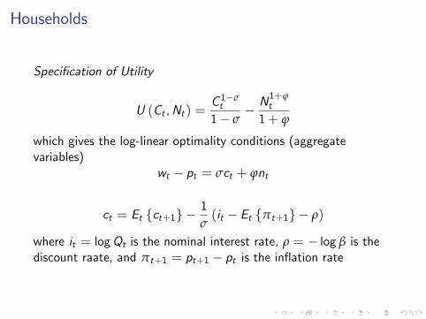
Households

Speci�cation of Utility

U (Ct ,Nt ) =C 1�σt

1� σ� N1+ϕ

t

1+ ϕ

which gives the log-linear optimality conditions (aggregatevariables)

wt � pt = σct + ϕnt

ct = Et fct+1g �1σ(it � Et fπt+1g � ρ)

where it = logQt is the nominal interest rate, ρ = � log β is thediscount raate, and πt+1 = pt+1 � pt is the in�ation rate

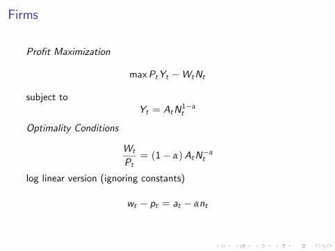
Firms

Pro�t Maximization

maxPtYt �WtNt

subject toYt = AtN1�α

t

Optimality Conditions

Wt

Pt= (1� α)AtN�α

t

log linear version (ignoring constants)

wt � pt = at � αnt

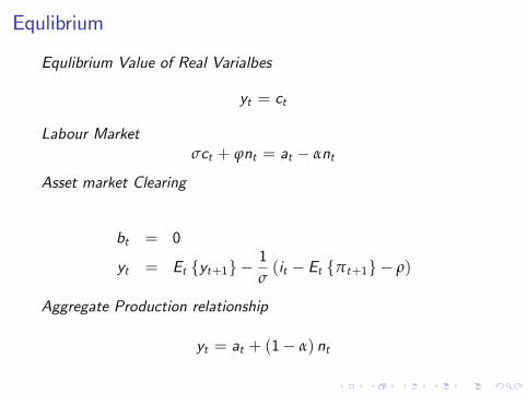
Equlibrium

Equlibrium Value of Real Varialbes

yt = ct

Labour Marketσct + ϕnt = at � αnt

Asset market Clearing

bt = 0

yt = Et fyt+1g �1σ(it � Et fπt+1g � ρ)

Aggregate Production relationship

yt = at + (1� α) nt

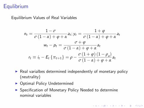
Equlibrium

Equilibrium Values of Real Variables

nt =1� σ

σ (1� α) + ϕ+ αat ; yt =

1+ ϕ

σ (1� α) + ϕ+ αat

wt � pt =σ+ ϕ

σ (1� α) + ϕ+ αat

rt � it � Et fπt+1g = ρ� σ (1+ ϕ) (1� ρa)

σ (1� α) + ϕ+ αat

I Real varialbes determined independently of monetary policy(neutrality)

I Optimal Policy UndeterminedI Speci�cation of Monetary Policy Needed to determinenominal variables

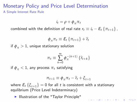
Monetary Policy and Price Level DeterminationA Simple Interest Rate Rule

it = ρ+ φππt

combined with the de�nition of real rate rt � it � Et fπt+1g ,

φππt � Et fπt+1g+brtif φπ > 1, unique stationary solution

πt �∞

∑k=0

φ�(k+1)π fbrt+kgif φπ < 1, any process πt satisfying

πt+1 � φππt �brt + ξt+1

where Et fξt+1g = 0 for all t is consistent with a stationaryequlibrium (Price Level Indeterminacy)

I Illustration of the "Taylor Principle"

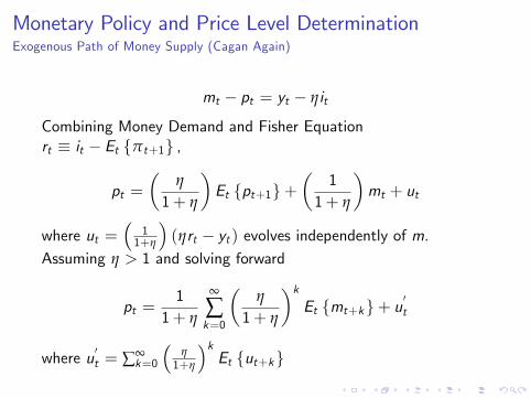
Monetary Policy and Price Level DeterminationExogenous Path of Money Supply (Cagan Again)

mt � pt = yt � ηit

Combining Money Demand and Fisher Equationrt � it � Et fπt+1g ,

pt =�

η

1+ η

�Et fpt+1g+

�1

1+ η

�mt + ut

where ut =�

11+η

�(ηrt � yt ) evolves independently of m.

Assuming η > 1 and solving forward

pt =1

1+ η

∞

∑k=0

�η

1+ η

�kEt fmt+kg+ u

0t

where u0t = ∑∞

k=0

�η1+η

�kEt fut+kg

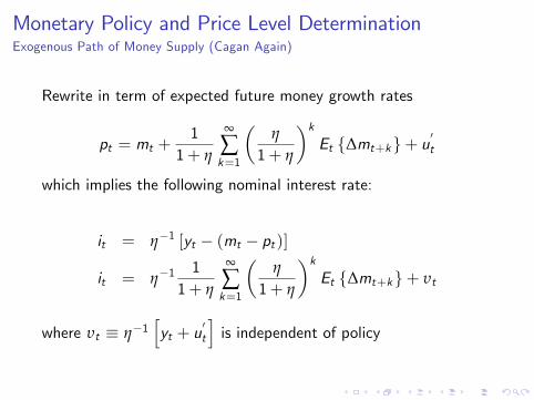
Monetary Policy and Price Level DeterminationExogenous Path of Money Supply (Cagan Again)

Rewrite in term of expected future money growth rates

pt = mt +1

1+ η

∞

∑k=1

�η

1+ η

�kEt f∆mt+kg+ u

0t

which implies the following nominal interest rate:

it = η�1 [yt � (mt � pt )]

it = η�11

1+ η

∞

∑k=1

�η

1+ η

�kEt f∆mt+kg+ υt

where υt � η�1hyt + u

0t

iis independent of policy

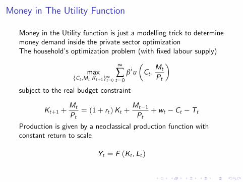
Money in The Utility Function

Money in the Utility function is just a modelling trick to determinemoney demand inside the private sector optimizationThe household�s optimization problem (with �xed labour supply)

maxfCt ,Mt ,Kt+1g∞

t=0

∞

∑t=0

βiu�Ct ,

Mt

Pt

�subject to the real budget constraint

Kt+1 +Mt

Pt= (1+ rt )Kt +

Mt�1Pt

+ wt � Ct � Tt

Production is given by a neoclassical production function withconstant return to scale

Yt = F (Kt , Lt )

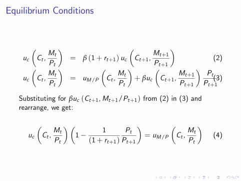
Equilibrium Conditions

uc

�Ct ,

Mt

Pt

�= β (1+ rt+1) uc

�Ct+1,

Mt+1

Pt+1

�(2)

uc

�Ct ,

Mt

Pt

�= uM/P

�Ct ,

Mt

Pt

�+ βuc

�Ct+1,

Mt+1

Pt+1

�PtPt+1(3)

Substituting for βuc (Ct+1,Mt+1/Pt+1) from (2) in (3) andrearrange, we get:

uc

�Ct ,

Mt

Pt

��1� 1

(1+ rt+1)PtPt+1

�= uM/P

�Ct ,

Mt

Pt

�(4)

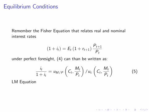
Equilibrium Conditions

Remember the Fisher Equation that relates real and nominalinterest rates

(1+ it ) = Et (1+ rt+1)Pt+1Pt

under perfect foresight, (4) can than be written as:

it1+ it

= uM/P

�Ct ,

Mt

Pt

�/uc

�Ct ,

Mt

Pt

�(5)

LM Equation

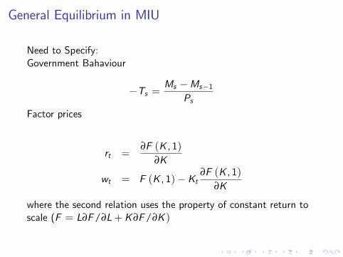
General Equilibrium in MIU

Need to Specify:Government Bahaviour

�Ts =Ms �Ms�1

PsFactor prices

rt =∂F (K , 1)

∂K

wt = F (K , 1)�Kt∂F (K , 1)

∂K

where the second relation uses the property of constant return toscale (F = L∂F/∂L+K∂F/∂K )

Steady State

To be consistent with the data a model including money shouldhave the following

I Neutrality of Money: the real equilibrium is independent ofthe money stock

I Superneutrality of money: the real equilibrium is independentof the money growth rate

Nominal Equilibrium

Mt/Mt�1 = 1+ σ

Pt/Pt�1 = 1+ π

Ct/Ct�1 = 1

Mt/Pt/Mt�1/Pt�1 = 1

π = σ

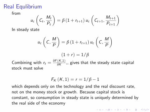
Real Equlibriumfrom

uc

�Ct ,

Mt

Pt

�= β (1+ rt+1) uc

�Ct+1,

Mt+1

Pt+1

�In steady state

uc

�C ,MP

�= β (1+ rt+1) uc

�C ,MP

�(1+ r) = 1/β

Combining with rt =∂F (K ,1)

∂K ,, gives that the steady state capitalstock must solve

FK (K , 1) = r = 1/β� 1which depends only on the technology and the real discount rate,not on the money stock or growth. Because capital stock isconstant, so consumption in steady state is uniquely determined bythe real side of the economy

C = F (K , 1)

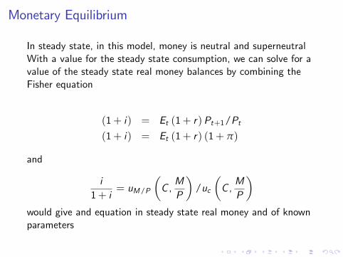
Monetary Equilibrium

In steady state, in this model, money is neutral and superneutralWith a value for the steady state consumption, we can solve for avalue of the steady state real money balances by combining theFisher equation

(1+ i) = Et (1+ r)Pt+1/Pt(1+ i) = Et (1+ r) (1+ π)

and

i1+ i

= uM/P

�C ,MP

�/uc

�C ,MP

�would give and equation in steady state real money and of knownparameters

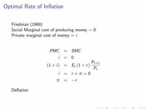
Optimal Rate of In�ation

Friedman (1969)Social Marginal cost of producing money = 0Private marginal cost of money = i

PMC = SMC

i = 0

(1+ i) = Et (1+ r)Pt+1Pt

i = r + π = 0

π = �r

De�ation

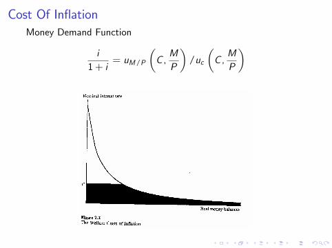
Cost Of In�ationMoney Demand Function

i1+ i

= uM/P

�C ,MP

�/uc

�C ,MP

�

Conclusions

I Basic Flexible Price Models Highlight:I The Role of ExpectationsI The Importance of Policy Design for Price DeterminationI Cost of In�ation (even when we have neutrality of money)

I Problems:I Money has no e¤ect on real variables (only welfare)I Friedman (1968) not realistic (De�ation is costly, but why?)