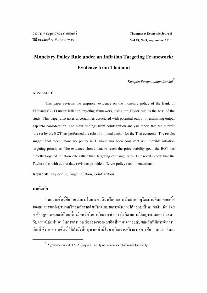
วารสารเศรษฐศาสตรธรรมศาสตร Thammasat Economic Journal ปท 28 ฉบบท 3 กนยายน 2553 Vol.28, No.3, September 2010

Monetary Policy Rule under an Inflation Targeting Framework: Evidence from Thailand

Kumpon Pornpattanapaisankul

ABSTRACT

This paper reviews the empirical evidence on the monetary policy of the Bank of Thailand (BOT) under inflation targeting framework, using the Taylor rule as the base of the study. This paper also takes uncertainties associated with potential output in estimating output gap into consideration. The main findings from cointegration analysis report that the interest rate set by the BOT has performed the role of nominal anchor for the Thai economy. The results suggest that recent monetary policy in Thailand has been consistent with flexible inflation targeting principles. The evidence shows that, to reach the price stability goal, the BOT has directly targeted inflation rate rather than targeting exchange rates. Our results show that the Taylor rules with output data revisions provide different policy recommendations.

Keywords: Taylor rule, Target inflation, Cointegration

บทคดยอ

บทความชนนศกษาแนวทางในการดาเนนนโยบายการเงนแบบกฎโดยผานอตราดอกเบยของธนาคารแหงประเทศไทยหลงจากดาเนนนโยบายการเงนภายใตกรอบเปาหมายเงนเฟอ โดยอาศยกฎของเทเลอรเปนเครองมอหลกในการวเคราะห อยางไรกตามการใชกฎของเทเลอร จะพบกบความไมแนนอนในการคานวณชองวางของผลผลตทหามาจากระดบผลผลตทมการจางงานเตมท ซงบทความชนน ไดคานงทปญหาเหลานในการวเคราะหดวย ผลการศกษาพบวา อตรา

A graduate student of M.A. program, Faculty of Economics, Thammasat University

144

ดอกเบยนโยบายทกาหนดโดยธนาคารแหงประเทศไทย ทาหนาทเปน nominal anchor ในการควบคมเงนเฟอ และสอดคลองกบ flexible inflation-targeting principlesโดยอาศยการวเคราะหความสมพนธระยะยาว การดาเนนนโยบายการเงนผานชองทางอตราดอกเบยของธนาคารแหงประเทศไทย เนนควบคมเงนเฟอโดยตรงมากกวาการควบคมการเคลอนไหวของอตราแลกเปลยนเพอบรรลเปาหมายเงนเฟอ นอกจากนผลการศกษายงพบวา เมอขอมลของผลผลตถกปรบแกกฎของเทเลอรใหขอเสนอแนะทางนโยบายทตางกน

คาสาคญ: กฎของเทเลอร, เปาหมายเงนเฟอ, ความสมพนธระยะยาว

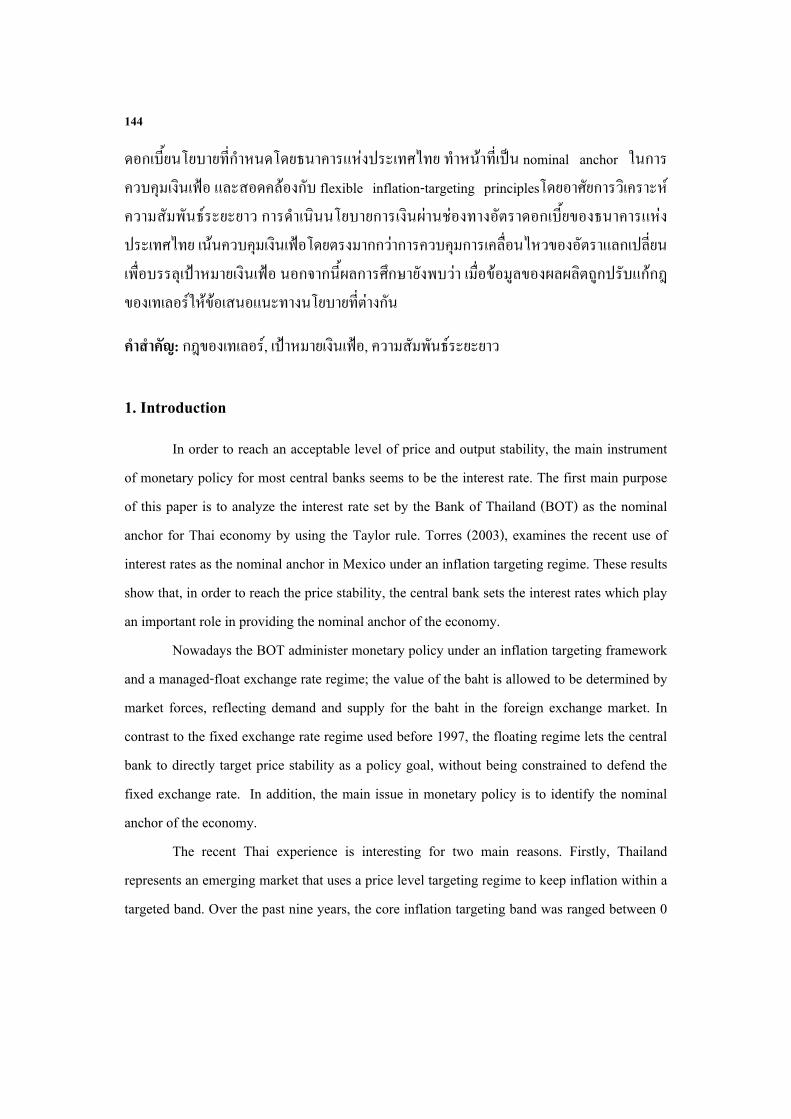
1. Introduction

In order to reach an acceptable level of price and output stability, the main instrument of monetary policy for most central banks seems to be the interest rate. The first main purpose of this paper is to analyze the interest rate set by the Bank of Thailand (BOT) as the nominal anchor for Thai economy by using the Taylor rule. Torres (2003), examines the recent use of interest rates as the nominal anchor in Mexico under an inflation targeting regime. These results show that, in order to reach the price stability, the central bank sets the interest rates which play an important role in providing the nominal anchor of the economy.

Nowadays the BOT administer monetary policy under an inflation targeting framework and a managed-float exchange rate regime; the value of the baht is allowed to be determined by market forces, reflecting demand and supply for the baht in the foreign exchange market. In contrast to the fixed exchange rate regime used before 1997, the floating regime lets the central bank to directly target price stability as a policy goal, without being constrained to defend the fixed exchange rate. In addition, the main issue in monetary policy is to identify the nominal anchor of the economy.

The recent Thai experience is interesting for two main reasons. Firstly, Thailand represents an emerging market that uses a price level targeting regime to keep inflation within a targeted band. Over the past nine years, the core inflation targeting band was ranged between 0

145

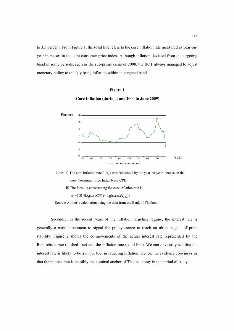
to 3.5 percent. From Figure 1, the solid line refers to the core inflation rate measured as year-on-year increases in the core consumer price index. Although inflation deviated from the targeting band in some periods, such as the sub-prime crisis of 2008, the BOT always managed to adjust monetary policy to quickly bring inflation within its targeted band.

Figure 1 Core Inflation (during June 2000 to June 2009)

-2

-1

0

1

2

3

4

00 01 02 03 04 05 06 07 08

the core inflation rate

Notes: i) The core inflation rate ( t ) was calculated by the year-on-year increase in the core Consumer Price Index (core CPI). ii) The formula constructing the core inflation rate is

12100*[log( ) log( )]t t tcoreCPI coreCPI Source: Author’s calculation using the data from the Bank of Thailand.

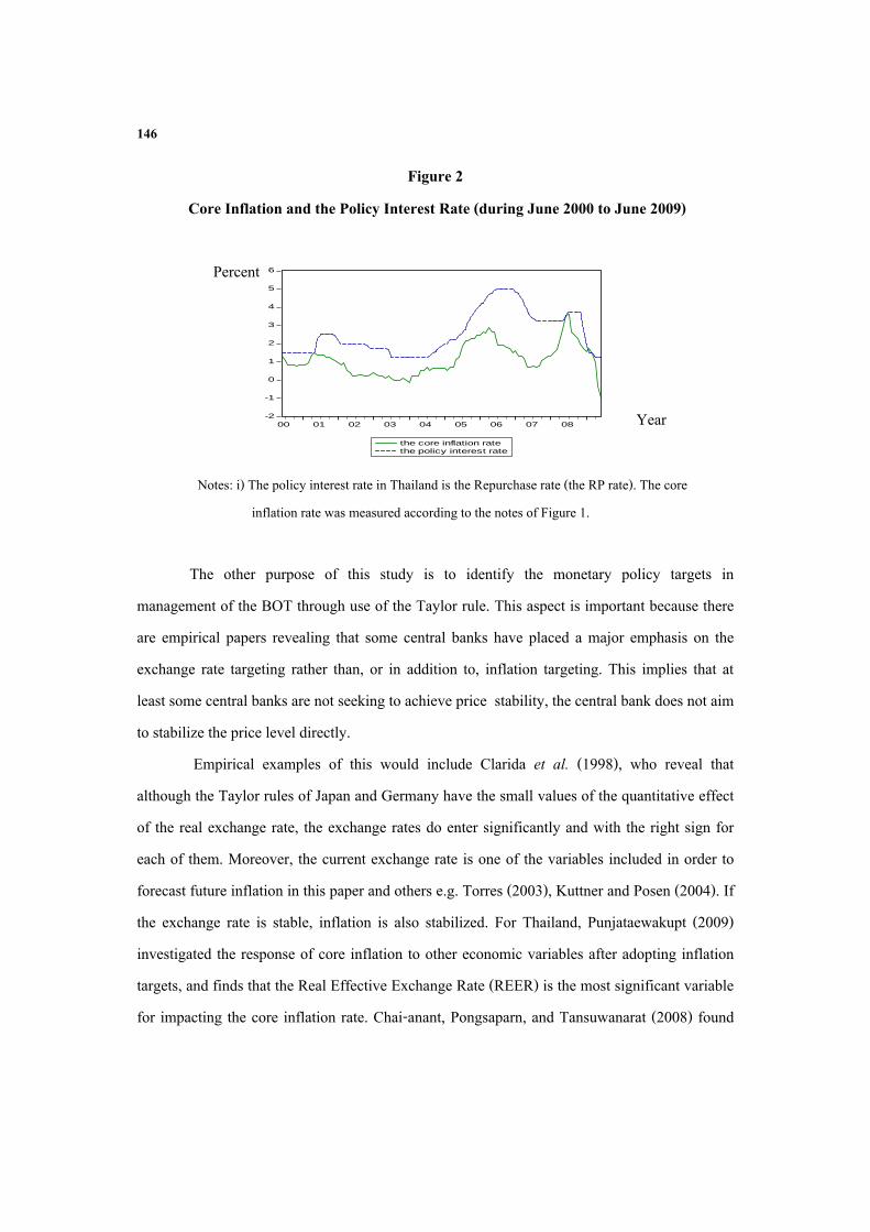
Secondly, in the recent years of the inflation targeting regime, the interest rate is generally a main instrument to signal the policy stance to reach an ultimate goal of price stability. Figure 2 shows the co-movements of the actual interest rate represented by the Repurchase rate (dashed line) and the inflation rate (solid line). We can obviously see that the interest rate is likely to be a major tool in reducing inflation. Hence, the evidence convinces us that the interest rate is possibly the nominal anchor of Thai economy in the period of study.

Percent

Year

146

Figure 2 Core Inflation and the Policy Interest Rate (during June 2000 to June 2009)

-2

-1

0

1

2

3

4

5

6

00 01 02 03 04 05 06 07 08

the core inflation ratethe policy interest rate

Notes: i) The policy interest rate in Thailand is the Repurchase rate (the RP rate). The core inflation rate was measured according to the notes of Figure 1.

The other purpose of this study is to identify the monetary policy targets in

management of the BOT through use of the Taylor rule. This aspect is important because there are empirical papers revealing that some central banks have placed a major emphasis on the exchange rate targeting rather than, or in addition to, inflation targeting. This implies that at least some central banks are not seeking to achieve price stability, the central bank does not aim to stabilize the price level directly.

Empirical examples of this would include Clarida et al. (1998), who reveal that although the Taylor rules of Japan and Germany have the small values of the quantitative effect of the real exchange rate, the exchange rates do enter significantly and with the right sign for each of them. Moreover, the current exchange rate is one of the variables included in order to forecast future inflation in this paper and others e.g. Torres (2003), Kuttner and Posen (2004). If the exchange rate is stable, inflation is also stabilized. For Thailand, Punjataewakupt (2009) investigated the response of core inflation to other economic variables after adopting inflation targets, and finds that the Real Effective Exchange Rate (REER) is the most significant variable for impacting the core inflation rate. Chai-anant, Pongsaparn, and Tansuwanarat (2008) found

Year

Percent

147

that, besides the role of exchange rate in terms of a channel of monetary policy transmission mechanism and a shock absorber, the exchange rate also takes an additional role in reducing inflation that is caused by an increase in oil and commodities prices. Khemangkorn, Mallikamas, and Sutthasri (2008) also found that in the past Thailand’s inflation dynamics were largely governed by supply distortions. All of these empirical findings reveal the strong relationship between the exchange rate and the inflation rate in the economy, which at the very least implies that the exchange rate stabilization may induce the price level stabilization.

In order to use the Taylor rule, we have to define potential output, which is seemed to be the main obstacle because of its uncertainty. Orphanides (1997) is the first paper that raises the issue of unreliable potential output data in estimating Taylor rules for the United States. He argues that the original Taylor rule relying on the ex-post data is based on unrealistic assumptions about the timeliness of data availability and ignores subsequent revisions. Thus, the Taylor rule is problematic in practice. Orphanides (1997) has emphasized the importance of using real time data, the data available to the central bank at the time that policy decisions are made. Kuttner and Posen (2004) also point out this problem in the case of Japan. Given the difficulty of revising the data over time, this is a substantial problem. Orphanides and van Norden (2002) propose quasi real time trends that are updated each period to construct the trends. For this reason, many papers mostly rely on the quasi real time output gap in order to construct the Taylor rules.

To address these questions, conventional papers estimated the Taylor rule in two ways. The backward-looking Taylor rule specification (i.e., the interest rate responds to current inflation and the output gap) is estimated using ordinary least square (OLS), while Clarida et al. (1998) propose the generalized method of moment (GMM) in estimating the forward-looking specification (i.e., the interest rate depends on the expected future inflation and the output gap). Although the OLS and GMM estimations seem to be appropriate, they estimate the Taylor rules without sufficient consideration of the integration properties of the time series, such that whether or not series contain a trend and whether that trend is deterministic or stochastic (i.e.,

148

the unit root problem). Unfortunately, the econometric time series used often do are not concerned with the stationary of the data used in estimation, causing potential spurious regressions. Papers estimating the Taylor rules generally do not take enough consideration on the appropriate unit root test. For instance, Torres (2003) uses the nonstationary data for a forward-looking framework in a GMM model.

Thus, Andrade and Divino (2005), Christensen and Nielsen (2003) dispute the contention in previous papers that if variables considered are non-stationary, it is not suitable to implement the usual estimations such as OLS and GMM. Moreover, Phillips and Perron (1988), Elliott, Rothenberg, and Stock (1996), and Ng and Perron (2001) suggest that the unit root test should be a powerful test that is robust to size and power distortions. And the maximum lag length set up should make the residual serially uncorrelated. They, for this reason, allow for GLS detrending of the data and the modified information criteria (MIC) yields the desirable size and power properties. Consequently, this paper aims to analyze the role of interest rate set by the BOT as the nominal anchor and to identify the behavior of the BOT in the monetary policy management under an inflation targeting framework by using the cointegration analysis.

2. Monetary Reaction Function

The main framework in this study discusses the Taylor rule specification which is closely specified along the lines of Clarida et al. (1998), and Andrade and Divino (2005). In order to use the Taylor rule in analyzing monetary policy, we assume that a short term interest rate is the main operating instrument of monetary policy for a central bank. The baseline Taylor rule can be characterized as follows:

* *[( ) ] [ ]t t t n t y t t ti i E E y

(1)

where i is the long run equilibrium nominal interest rate, *

t t ty y y , ty is real output, t n is the inflation rate between periods t and t n .

and ty are targets for inflation and

149

output, respectively. ty is the potential output level. E is the expected value of a variable. The central bank adjusts the target nominal interest rate ( ti ) based on the information set available at time t represented by t .

The critical point for monetary policy analysis is the magnitude of the parameter . If

> 1, the Taylor rule suggests that the nominal interest rate rises sufficiently to let the real interest rate increases as well. With 0 1 , the real rate will reinforce the inflation pressure i.e. although the nominal rate is raised in response to a rise in inflation, it does not sufficiently increase to keep the real rate from declining. Therefore, when > 1, it is not unreasonable to say that monetary policy works as an automatic stabilizer of inflation and the interest rate serves as a nominal anchor of the economy. For the parameter y , Eq. (1) shows that the critical value is 0. When 0y , the interest rate tries to stabilize output and avoid pressure on future inflation. In general, the estimated magnitude of the parameters and y describe whether a central bank takes the inflationary pressures from supply side into consideration. If there is no the output gap in the policy rule, we call this characteristic as strict inflation targeting. On the contrary, if both inflation and output gap estimates are statistically greater than 1, and greater than 0, respectively, the interest rate seemingly plays a role as the nominal anchor in the economy. We call this characteristic as flexible inflation targeting.

The empirical specification of the Taylor rule like Eq. (1) may not be suitable. A concern is that Eq. (1) cannot capture the tendency of the central bank to smooth changes in interest rates. This would be the case if the central bank is not concerned about the loss of credibility from large policy changes, or the fear that capital markets are disturbed by changes of interest rate, etc. Accordingly, it is more desirable to assume that the actual nominal rate ( ti ) partially adjusts to the targeted interest rate ( ti ), as follows:

1(1 )t t t ti i i v (2)

150

where [0,1] captures the degree of interest rate smoothing, tv is an exogenous interest rate shock. We assume that tv is i.i.d.

Putting the targeted interest rate Eq. (1) into the smoothing mechanism Eq. (2) yields

1 (1 ) [ ] [ ]t t o t t n t y t t t ti i E E y v (3)

where * *o i . The policy rule in Eq. (3) should be estimated by the GMM if the

variables are stationary. However, if the variables are integrated of first order, we should then investigate the cointegration properties of the non-stationary series. Then, the long run solution of Eq. (3) can be characterized as;

1 (1 ) ( [ ]) [ ]t t o t n t y t t ti i E E y v

after rearranging, we get o yi y (4)

where 1, (1 )t

t t

vi i i and

It is argued that the state variables in the baseline Taylor rule above ignore the characteristics of an open economy, which may be far from optimal in some circumstances. For instance, the central bank may pursue monetary policy to maintain an exchange rate within some band. The exchange rate may thus have influenced policy. Although the real exchange rate is but one of the other important factors affecting a small open economy, many papers assume that central banks target real exchange rates for following reasons. First, the central bank can target the real exchange rate to reach the price stability, if the inflation rate is significantly affected by the increases in oil and commodity prices. The second reason for adding the real exchange rates is a central banks desire to hold purchasing power parity (PPP) stable. Hence, we replace the relation for the target given by Eq. (1) with the following:

151

* *[( ) ] [ ] [ ]t t t n t y t t t q t t ti i E E y E q

(5) where tq is the real exchange rate. We then proceed to estimate the augmented model in the same fashion as the baseline, and the long run relationship can be written as follow:

o y qi y q (6)

3. Literature Review

This section provides the empirical aspect for analyzing monetary policy and interest rates in various countries by using the Taylor rule. The papers are consisting of the works acre several geographic areas. In Japan, tests were done by McCallum (2000), Clarida et al. (1998), Andrade and Divino (2003), Kuttner and Posen (2004), Bernake and Gertler (1999)). In the U.S. , Clarida et al. (1998), Bernake and Gertler (1999) ), in the Euro area Adema (2004), Belke and Klose (2009) ), in Mexico Torres (2003). Finally, in Thailand Suthiwat (2002).

There are three main issues for the Taylor rule estimation based on the unreliability of output gap estimates. The so-called model uncertainty, the first dimension, depends on potential output definitions. Potential output or the output gap provides the important information about an appropriate monetary policy setting but potential output is unobservable. Although there are many papers mentioned in this section, the potential output estimations can be commonly categorized into three strategies: the linear trend, the quadratic trend, and the HP filter. All three of these gap estimate techniques are well known and widely used because they are easy to implement in a practical manner. That is the methods depend solely on output data. We call this characteristic the univariate approach. However, there are other output gap estimates used, such as the production function, the unobserved component etc. Interestingly, Kuttner and Posen (2004)’s review of related papers in the case of Japan shows that all of papers use the univariate approach. In addition, the reviewed papers apply several potential output definitions in their works.

152

The second issue is the choice between a real time and ex-post revised output gap estimates. Orphandines (1997) shows that the policy rules that based on real time output gap estimates differ considerably from the others obtained with the ex-post revised data.1 Consequently, Bernake and Gertler (1999), Kuttner and Posen (2004), Adema (2004), and Molodtsova and Papell (2008) take the informational problem into account by constructing the quasi-real time output gap estimates. According to Orphandines and van Norsen (2002), if the informational problem is considered due to the data revision, we use the quasi-real time data instead of the true real time estimate. Moreover, the real time output data are not available in many countries. Belke and Klose (2009) compare both ex-post and real time data in estimating Taylor rules for the European Central Bank (ECB), whereas Kuttner and Posen (2004) analyze both ex-post revised and quasi-real time data with different gap estimates.

Finally, the papers mostly rely on the forward- looking Taylor rule rather than the current information that is called the backward or contemporaneous-looking. Many papers such as Kuttner and Posen (2004), Belke and Klose (2009) apply both types of looking in their studies in order to compare the models ability to explain the actual interest rate. Each paper gives us the general agreement that the forward-looking is more attractive because it can reduce the informational problem.

After we have specified the Taylor rule, it is necessary to describe the estimation procedures of the related papers. The papers apply an Ordinary Least Squared (OLS) estimator for the contemporaneous-looking Taylor rule. The forward-looking models are usually estimated by Generalized Method of Moment (GMM), while Orphanides (1997) applies two stage least square (2 SLS). Clarida et al. (1998) is the first paper to apply GMM for the forward-looking model because this model includes the expected inflation deviation from its target and the expected output gap. There are two main concerns with this model. Firstly, the inflation forecast information in not available to most central banks. Secondly, information

1 Orphanides (1997) constructs a data base of current quarter forecasts of the quantities required by the

Taylor rule based only on information available in real time.

153

regarding the central bank’ expected output gap is also not available. Consequently, future values of the variables are instrumented with the lagged values that help to forecast future inflation.

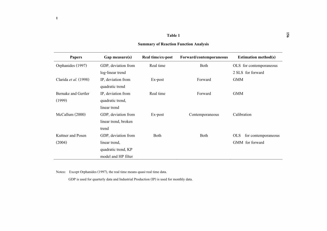
Andrade and Divino (2005), and Christensen and Nielsen (2003)2 argue that the use of nonstationary series (i.e., I (1)) in a GMM model without testing the cointegration among the series limits the asymptotic property of the estimator. So, we should apply the cointegration analysis, if all variables are not stationary. Table 1 reports the summary for various papers mentioned in this section.

4. Potential Output Uncertainties and Monetary Policy Rule

One of key variables that can be used to predict future inflation is potential output3, which represents the output level when all prices and wages are fully employed. Unfortunately, potential output is not directly observed, which causes the main obstacle for the central bank in conducting the policy. The inability to observe it is commonly called the potential output uncertainty. Frequently, most macroeconomic researchers ignore the considerable uncertainty in constructing the output gap. This may create a difficulty for economic stabilization policy such as the Taylor rule, which requires reliable output gap estimates when the interest rate decisions are being made. As a result, wrong information can mislead a central bank when choosing the target interest rate. Commonly, there are three types of uncertainty in the estimation of potential output, which lead to the problems with the measurement of the output gap: model uncertainty, statistical uncertainty, and data uncertainty.

(A) Model Uncertainty: This uncertainty governs the appropriate empirical definition of potential output. Although several methods have been proposed to measure potential output, we can broadly classify them into two approaches: (1) the univariate approach; the fitted linear

2 Among authors, cointegration analysis is used in Gerlach-Kristen (2003), Osterholm (2005), Eleftheriou

(2009). This list is not exhaustive. 3 See Chuenchoksan et al. (2008)

154

trend, the fitted quadratic trend, and the Hodrick-Prescott (HP) Filter and (2) other approaches; the production function model, unobserved component model, structural VAR, and Dynamic stochastic general equilibrium (DSGE) models. Different methods for constructing potential output give us different outcomes and different policy implications.

(B) Statistical Uncertainty: This uncertainty governs the appropriate of sample size in the potential output estimation. This is due to the model having unknown parameters which have to be estimated from small samples .If we re-estimate the parameters, the value will be changed by revised data and longer data sets. In retrospect, we prefer the longer time series rather than the shorter for getting consistent estimates.

(C) Data Uncertainty: This is due to the fact that data about output and other macroeconomic variables are not available in real time, and when the data does become available, it typically needs multiple revisions over time. This makes estimating and using the Taylor rule containing the output gap information problematic. Orphanides (1997) gives some reasons for the impact of informational problem in the Taylor rule analysis. Firstly, the original Taylor rule allows the target interest rate to depend on current information of the inflation rate and the output gap which is not available in the time when the central bank chooses the targeted policy. Accordingly, it is not accurate to say that this rule is operational in practice. Secondly, since the data used to calculate potential output are revised, the value of potential output will be changed relative to the unrevised or real time data. Thus, the target interest rate will also be different between these two types of data.

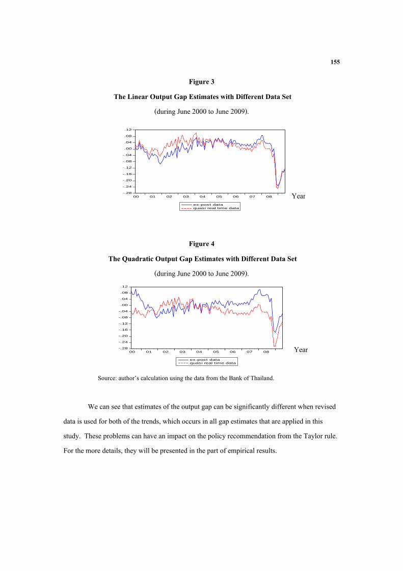
Figure 3-4 shows the extent of the revision of the Thai output gap estimates of the linear trend, and the quadratic trend, respectively. As expected, the gap estimates varies when the information is revised.

155

Figure 3 The Linear Output Gap Estimates with Different Data Set

(during June 2000 to June 2009).

Figure 4

The Quadratic Output Gap Estimates with Different Data Set (during June 2000 to June 2009).

-.28

-.24

-.20

-.16

-.12

-.08

-.04

.00

.04

.08

.12

00 01 02 03 04 05 06 07 08

ex-post dataquasi real time data

Source: author’s calculation using the data from the Bank of Thailand.

We can see that estimates of the output gap can be significantly different when revised

data is used for both of the trends, which occurs in all gap estimates that are applied in this study. These problems can have an impact on the policy recommendation from the Taylor rule. For the more details, they will be presented in the part of empirical results.

Year

-.28

-.24

-.20

-.16

-.12

-.08

-.04

.00

.04

.08

.12

00 01 02 03 04 05 06 07 08

ex-post dataquasi real time data

Year

1

Table 1 Summary of Reaction Function Analysis

Papers Gap measure(s) Real time/ex-post Forward/contemporaneous Estimation method(s) Orphanides (1997) GDP, deviation from

log-linear trend Real time Both OLS for contemporaneous

2 SLS for forward Clarida et al. (1998) IP, deviation from

quadratic trend Ex-post Forward GMM

Bernake and Gertler (1999)

IP, deviation from quadratic trend, linear trend

Real time Forward GMM

McCallum (2000) GDP, deviation from linear trend, broken trend

Ex-post Contemporaneous Calibration

Kuttner and Posen (2004)

GDP, deviation from linear trend, quadratic trend, KP model and HP filter

Both Both OLS for contemporaneous GMM for forward

Notes: Except Orphanides (1997), the real time means quasi-real time data. GDP is used for quarterly data and Industrial Production (IP) is used for monthly data.

156

2

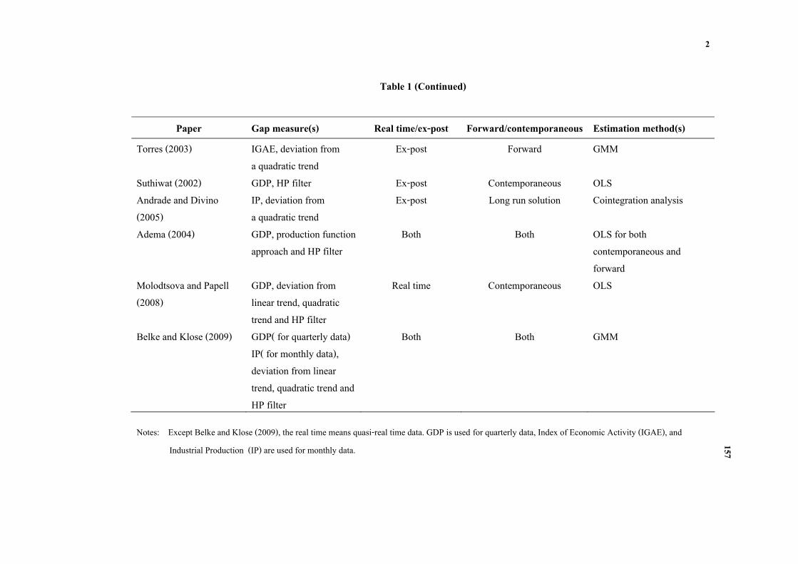
Table 1 (Continued)

Paper Gap measure(s) Real time/ex-post Forward/contemporaneous Estimation method(s) Torres (2003) IGAE, deviation from

a quadratic trend Ex-post Forward GMM

Suthiwat (2002) GDP, HP filter Ex-post Contemporaneous OLS Andrade and Divino (2005)

IP, deviation from a quadratic trend

Ex-post Long run solution Cointegration analysis

Adema (2004) GDP, production function approach and HP filter

Both Both OLS for both contemporaneous and forward

Molodtsova and Papell (2008)

GDP, deviation from linear trend, quadratic trend and HP filter

Real time Contemporaneous OLS

Belke and Klose (2009) GDP( for quarterly data) IP( for monthly data), deviation from linear trend, quadratic trend and HP filter

Both Both GMM

Notes: Except Belke and Klose (2009), the real time means quasi-real time data. GDP is used for quarterly data, Index of Economic Activity (IGAE), and Industrial Production (IP) are used for monthly data.

157

158

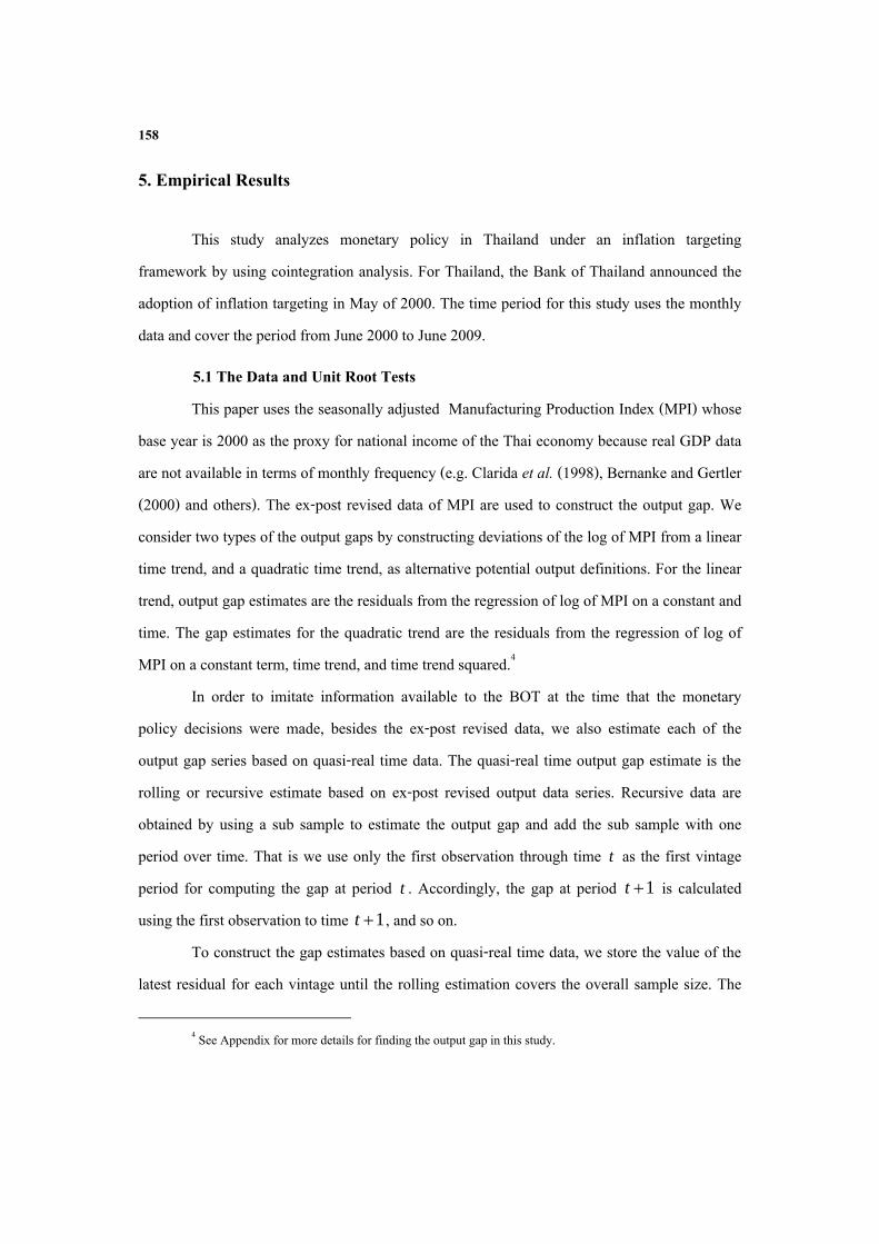
5. Empirical Results

This study analyzes monetary policy in Thailand under an inflation targeting framework by using cointegration analysis. For Thailand, the Bank of Thailand announced the adoption of inflation targeting in May of 2000. The time period for this study uses the monthly data and cover the period from June 2000 to June 2009.

5.1 The Data and Unit Root Tests This paper uses the seasonally adjusted Manufacturing Production Index (MPI) whose

base year is 2000 as the proxy for national income of the Thai economy because real GDP data are not available in terms of monthly frequency (e.g. Clarida et al. (1998), Bernanke and Gertler (2000) and others). The ex-post revised data of MPI are used to construct the output gap. We consider two types of the output gaps by constructing deviations of the log of MPI from a linear time trend, and a quadratic time trend, as alternative potential output definitions. For the linear trend, output gap estimates are the residuals from the regression of log of MPI on a constant and time. The gap estimates for the quadratic trend are the residuals from the regression of log of MPI on a constant term, time trend, and time trend squared.4

In order to imitate information available to the BOT at the time that the monetary policy decisions were made, besides the ex-post revised data, we also estimate each of the output gap series based on quasi-real time data. The quasi-real time output gap estimate is the rolling or recursive estimate based on ex-post revised output data series. Recursive data are obtained by using a sub sample to estimate the output gap and add the sub sample with one period over time. That is we use only the first observation through time t as the first vintage period for computing the gap at period t . Accordingly, the gap at period 1t is calculated using the first observation to time 1t , and so on.

To construct the gap estimates based on quasi-real time data, we store the value of the latest residual for each vintage until the rolling estimation covers the overall sample size. The

4 See Appendix for more details for finding the output gap in this study.

159

output gap for the first period is calculated using MPI series from July 1997 to June 2000 because the Asian financial crisis in Thailand began in July 1997 after the Thai government decided to float the Thai baht by cutting its peg to the U.S. dollar. In retrospect, we are worried about structural changes associated with the output growth slowdown, and prefer to use longer series. The difference between the first estimate of the output gap for a given time period and the ex-post estimate based on the whole sample shows the size of revisions of the real time output gap due to statistical uncertainty.

The inflation rate is based on a year-on-year increase in core CPI because the BOT are more concerned about the medium term trend in conducting the policy. The short term interest ( )ti , represented by the repurchase rate (the RP), was used as the policy interest rate but the policy interest rate was switched from the 14-day RP rate to the 1-day RP rate on January 2007.

Finally, the real exchange rate is computed as the log of the real effective exchange rate (REER). Under the inflation targeting framework and the managed float, one of the main tasks of the BOT is to sustain the stable value of the Thai baht in order to maintain the competitiveness of the Thai economy. The main reason for choosing the REER is, rather than including only the bilateral exchange rate with the dollar, it comprises currencies of other important trading partners. An increase in the value of the REER means that the Thai baht has appreciated.

To investigate the stochastic properties of the data series, the time series analysis of this paper begins with the unit root test. We test for the series of the interest rate ( )ti , the inflation rate ( t ), the real effective exchange rate ( tq ), and four types of output gap estimate; for the ex-post revised data the output gap estimates from the linear time trend ( el

ty ), and the quadratic time trend ( eq

ty ),whereas for the quasi-real time data output gap estimates from the linear time trend ( ql

ty~ ) , and the quadratic time trend ( qqty~ ).

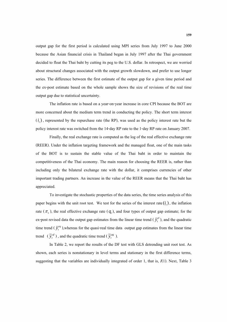
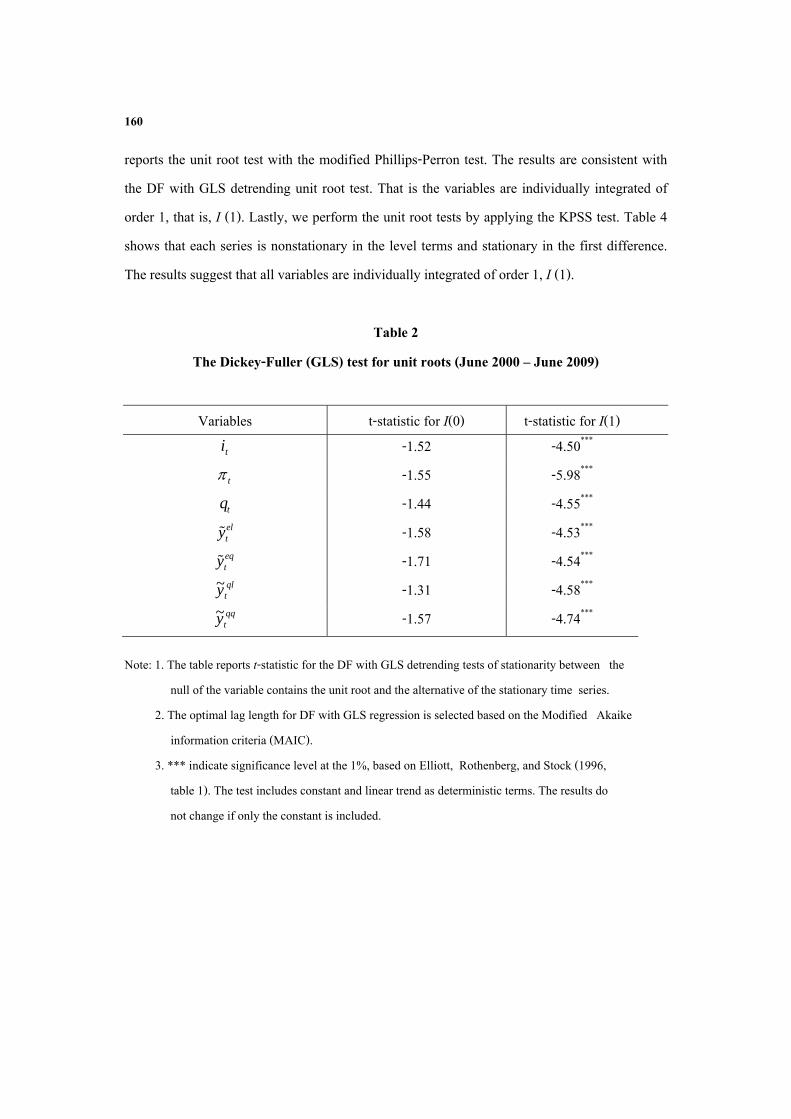
In Table 2, we report the results of the DF test with GLS detrending unit root test. As shown, each series is nonstationary in level terms and stationary in the first difference terms, suggesting that the variables are individually integrated of order 1, that is, I(1). Next, Table 3

160

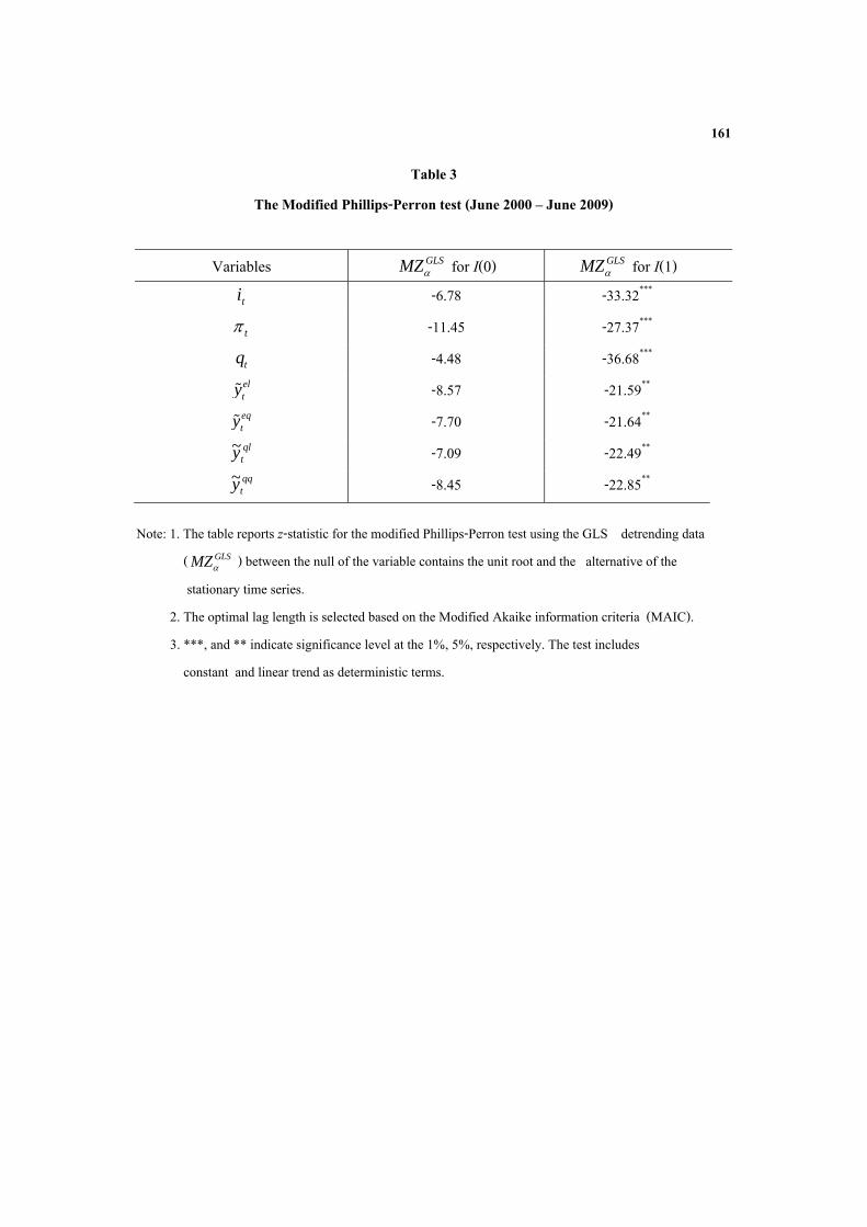
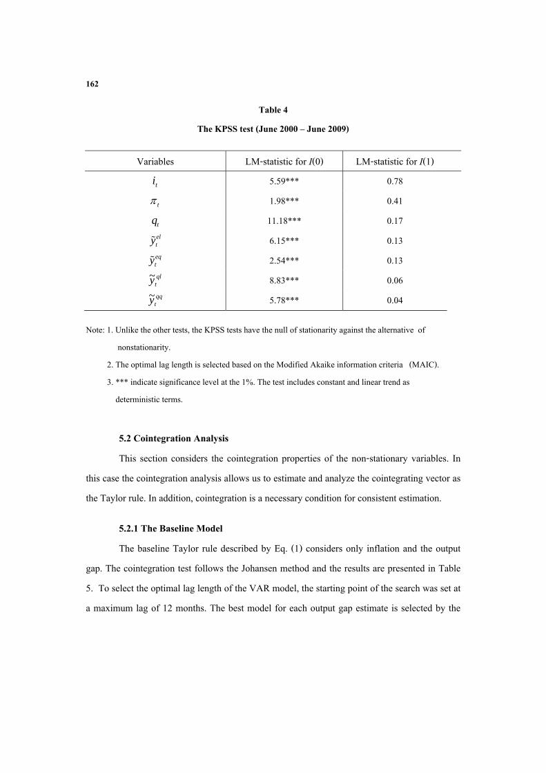
reports the unit root test with the modified Phillips-Perron test. The results are consistent with the DF with GLS detrending unit root test. That is the variables are individually integrated of order 1, that is, I (1). Lastly, we perform the unit root tests by applying the KPSS test. Table 4 shows that each series is nonstationary in the level terms and stationary in the first difference. The results suggest that all variables are individually integrated of order 1, I (1).

Table 2 The Dickey-Fuller (GLS) test for unit roots (June 2000 – June 2009)

Variables t-statistic for I(0) t-statistic for I(1)

ti -1.52 -4.50***

t -1.55 -5.98***

tq -1.44 -4.55*** elty -1.58 -4.53***

eqty -1.71 -4.54***

qlty~ -1.31 -4.58***

qqty~ -1.57 -4.74***

Note: 1. The table reports t-statistic for the DF with GLS detrending tests of stationarity between the null of the variable contains the unit root and the alternative of the stationary time series. 2. The optimal lag length for DF with GLS regression is selected based on the Modified Akaike information criteria (MAIC). 3. *** indicate significance level at the 1%, based on Elliott, Rothenberg, and Stock (1996, table 1). The test includes constant and linear trend as deterministic terms. The results do not change if only the constant is included.

161

Table 3 The Modified Phillips-Perron test (June 2000 – June 2009)

Variables GLSMZ for I(0) GLSMZ for I(1) ti -6.78 -33.32*** t -11.45 -27.37*** tq -4.48 -36.68*** elty -8.57 -21.59** eqty -7.70 -21.64** qlty~ -7.09 -22.49** qqty~ -8.45 -22.85**

Note: 1. The table reports z-statistic for the modified Phillips-Perron test using the GLS detrending data ( GLSMZ ) between the null of the variable contains the unit root and the alternative of the stationary time series. 2. The optimal lag length is selected based on the Modified Akaike information criteria (MAIC). 3. ***, and ** indicate significance level at the 1%, 5%, respectively. The test includes constant and linear trend as deterministic terms.

162

Table 4 The KPSS test (June 2000 – June 2009)

Variables LM-statistic for I(0) LM-statistic for I(1)

ti 5.59*** 0.78

t 1.98*** 0.41

tq 11.18*** 0.17 elty 6.15*** 0.13 eqty 2.54*** 0.13 qlty~ 8.83*** 0.06 qqty~ 5.78*** 0.04

Note: 1. Unlike the other tests, the KPSS tests have the null of stationarity against the alternative of nonstationarity. 2. The optimal lag length is selected based on the Modified Akaike information criteria (MAIC). 3. *** indicate significance level at the 1%. The test includes constant and linear trend as deterministic terms.

5.2 Cointegration Analysis This section considers the cointegration properties of the non-stationary variables. In

this case the cointegration analysis allows us to estimate and analyze the cointegrating vector as the Taylor rule. In addition, cointegration is a necessary condition for consistent estimation.

5.2.1 The Baseline Model The baseline Taylor rule described by Eq. (1) considers only inflation and the output

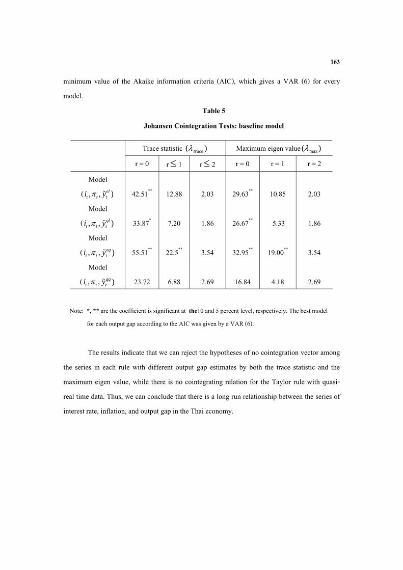
gap. The cointegration test follows the Johansen method and the results are presented in Table 5. To select the optimal lag length of the VAR model, the starting point of the search was set at a maximum lag of 12 months. The best model for each output gap estimate is selected by the

163

minimum value of the Akaike information criteria (AIC), which gives a VAR (6) for every model.

Table 5 Johansen Cointegration Tests: baseline model

Trace statistic )( trace Maximum eigen value )( max r = 0 r 1 r 2 r = 0 r = 1 r = 2

Model ( , , )el

t t ti y

42.51**

12.88

2.03

29.63**

10.85

2.03 Model

( , , )qlt t ti y

33.87*

7.20

1.86

26.67**

5.33

1.86

Model ( , , )eq

t t ti y

55.51**

22.5**

3.54

32.95**

19.00**

3.54 Model

( , , )qqt t ti y

23.72

6.88

2.69

16.84

4.18

2.69

Note: *, ** are the coefficient is significant at the10 and 5 percent level, respectively. The best model for each output gap according to the AIC was given by a VAR (6).

The results indicate that we can reject the hypotheses of no cointegration vector among

the series in each rule with different output gap estimates by both the trace statistic and the maximum eigen value, while there is no cointegrating relation for the Taylor rule with quasi-real time data. Thus, we can conclude that there is a long run relationship between the series of interest rate, inflation, and output gap in the Thai economy.

164

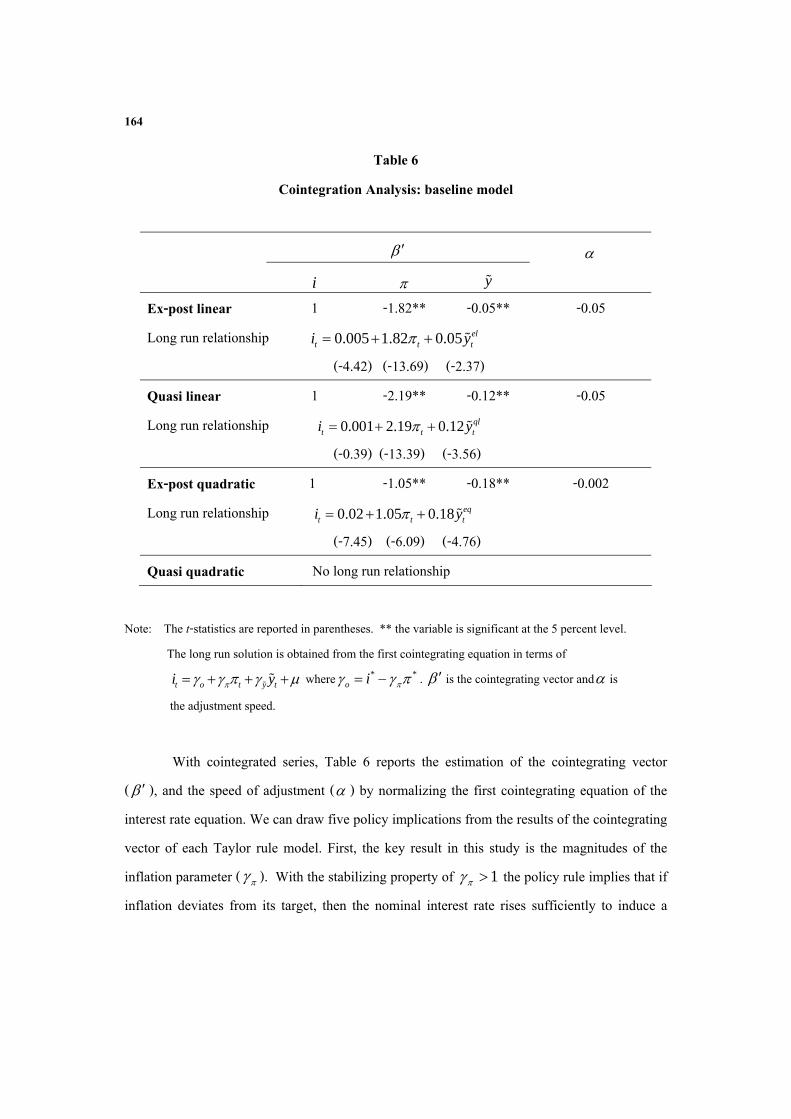
Table 6 Cointegration Analysis: baseline model

i y

Ex-post linear 1 -1.82** -0.05** -0.05 Long run relationship 0.005 1.82 0.05 el

t t ti y (-4.42) (-13.69) (-2.37)

Quasi linear 1 -2.19** -0.12** -0.05 Long run relationship 0.001 2.19 0.12 ql

t t ti y (-0.39) (-13.39) (-3.56)

Ex-post quadratic 1 -1.05** -0.18** -0.002 Long run relationship 0.02 1.05 0.18 eq

t t ti y (-7.45) (-6.09) (-4.76)

Quasi quadratic No long run relationship

Note: The t-statistics are reported in parentheses. ** the variable is significant at the 5 percent level. The long run solution is obtained from the first cointegrating equation in terms of t o t y ti y where * *

o i . is the cointegrating vector and is the adjustment speed.

With cointegrated series, Table 6 reports the estimation of the cointegrating vector

( ), and the speed of adjustment ( ) by normalizing the first cointegrating equation of the interest rate equation. We can draw five policy implications from the results of the cointegrating vector of each Taylor rule model. First, the key result in this study is the magnitudes of the inflation parameter ( ). With the stabilizing property of 1 the policy rule implies that if inflation deviates from its target, then the nominal interest rate rises sufficiently to induce a

165

change in the real interest rate. This result suggests that monetary policy in Thailand, through its effect on interest rates, has played the role of nominal anchor for the economy. This is consistent with Torres (2003). Regardless of which potential output proxy is used, the inflation parameter ( ) always has the desired value. For instance, in the case of the use of output gap based on ex-post linear time trend, equals 1.82. This means that the BOT responds to a rise in inflation of one percent by raising the real rate 82 basis points. In addition, the so-called Taylor principle holds in every case we calculated, regardless of the different output gap estimates.

Second, the estimate of the coefficient on the output gap ( y ) enters significantly with the right sign in all Taylor rule models. The rule with ex-post revised data when the output gap is estimated from a linear trend: y equals to 0.05. Thus, holding constant inflation, a one percent rise in the output gap induces the BOT to increase nominal (and thus real) interest rate by 5 basis points. y is positive and significant. This suggests that movements in the interest rate have prevented the presence of supply inflationary pressures. Nonetheless, in all models, the output gap estimates are uniformly small. Therefore, the one conclusion that seems to be robust to choice of output gap proxy is that, from 2000 to 2009, Thai monetary policy tended to be dominated by inflationary concerns, not the output gap.

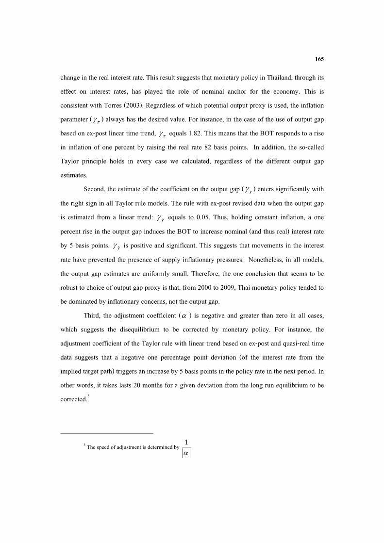
Third, the adjustment coefficient ( ) is negative and greater than zero in all cases, which suggests the disequilibrium to be corrected by monetary policy. For instance, the adjustment coefficient of the Taylor rule with linear trend based on ex-post and quasi-real time data suggests that a negative one percentage point deviation (of the interest rate from the implied target path) triggers an increase by 5 basis points in the policy rate in the next period. In other words, it takes lasts 20 months for a given deviation from the long run equilibrium to be corrected.5

5 The speed of adjustment is determined by 1

166

Fourth, we also obtain a plausible estimate of the long run nominal interest rate ( *i ). In this case we take the inflation target ( * ) equals to 1.75 percent, which is the official target’s mid-point, given that the BOT target for core inflation of 0-3.5 percent during this period. From * *

o i , the rule with linear trend based on ex-post and quasi-real time data implies a value for *i is 3.19, 3.83, respectively, while the rule with quadratic trend based on ex-post revised data implies a value for *i is 1.86. According to Taylor (1993), he calibrates the value of *i equals to 4 percent. We can see that, in this study, the Taylor rules based on linear trend provides more reasonable estimates than the quadratic trend.

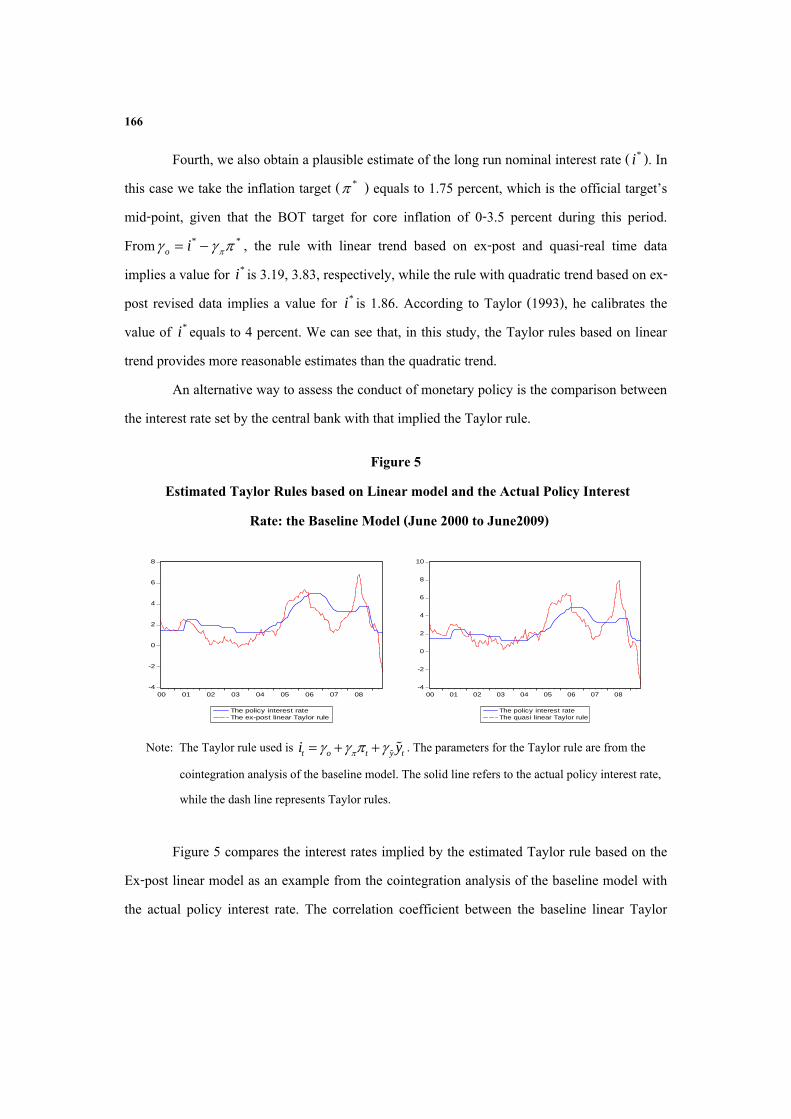
An alternative way to assess the conduct of monetary policy is the comparison between the interest rate set by the central bank with that implied the Taylor rule.

Figure 5 Estimated Taylor Rules based on Linear model and the Actual Policy Interest

Rate: the Baseline Model (June 2000 to June2009)

-4

-2

0

2

4

6

8

00 01 02 03 04 05 06 07 08

The policy interest rateThe ex-post linear Taylor rule

-4

-2

0

2

4

6

8

10

00 01 02 03 04 05 06 07 08

The policy interest rateThe quasi linear Taylor rule

Note: The Taylor rule used is t o t y ti y . The parameters for the Taylor rule are from the cointegration analysis of the baseline model. The solid line refers to the actual policy interest rate, while the dash line represents Taylor rules.

Figure 5 compares the interest rates implied by the estimated Taylor rule based on the Ex-post linear model as an example from the cointegration analysis of the baseline model with the actual policy interest rate. The correlation coefficient between the baseline linear Taylor

167

rules based on ex-post revised data and the actual policy interest rate is 0.7465, which is higher than any other baseline model. In other words, the Taylor rule based on ex-post linear model appears to have been consistently with the actual interest rate (i.e., monetary policy behavior) better than the rule using quadratic trends and quasi-real time data.6 This is due to the fact that the linear trend well captures the path of MPI series in this period. This finding is analogous to Orphanides (1997). Some of the most conspicuous differences between the ex-post revised and the quasi-real time estimates of the output gap occurred during the onset of the sub-prime crisis, when the quasi-real time measures implies shaper interest rate reduction was observed in the ex-post data.7

Lastly, using quasi-real time data instead of ex-post revised data in the cointegration analysis consistently yielded large and significant estimates of , i.e., greater than one. However, the magnitude of the output gap parameter is quite small. For a linear time trend, when we use of quasi-real time data in estimating the output gap, the parameters become higher. This implies the presence of the flexible inflation targeting principle.. It is essential to rely on quasi-real time data; otherwise this would lead to misleading views on monetary policy. Hence, we should be prudent with the interpretation of the Taylor rules in practice.

Generally, the results summarized above are consistent with those of Kuttner and Posen (2004), and Adema (2004), who examine the inherent uncertainty of the Taylor rule. So, we should be prudent with the interpretation of the estimated Taylor rules. In addition, it is worth keeping in mind that it is hard to gauge the optimality of the coefficients of a monetary policy reaction function such as the Taylor rule. Nevertheless, the Taylor rule is still useful for central banks in communicating their intentions and providing a benchmark for the current policy stance.

6 Plots for the other models can be seen in the full text version. 7 The results are also not changed for the Taylor rules with the quadratic trend.

168

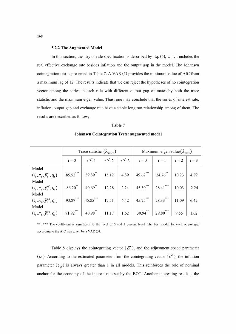
5.2.2 The Augmented Model In this section, the Taylor rule specification is described by Eq. (5), which includes the

real effective exchange rate besides inflation and the output gap in the model. The Johansen cointegration test is presented in Table 7. A VAR (5) provides the minimum value of AIC from a maximum lag of 12. The results indicate that we can reject the hypotheses of no cointegration vector among the series in each rule with different output gap estimates by both the trace statistic and the maximum eigen value. Thus, one may conclude that the series of interest rate, inflation, output gap and exchange rate have a stable long run relationship among of them. The results are described as follow;

Table 7 Johansen Cointegration Tests: augmented model

Trace statistic )( trace Maximum eigen value )( max r = 0 r 1 r 2 r 3 r = 0 r = 1 r = 2 r = 3 Model ( , , , )el

t t t ti y q

85.52***

39.89**

15.12

4.89

49.62***

24.76**

10.23

4.89 Model ( , , , )ql

t t t ti y q

86.20**

40.69**

12.28

2.24

45.50***

28.41***

10.03

2.24 Model ( , , , )eq

t t t ti y q

93.87***

45.85***

17.51

6.42

45.75***

28.33***

11.09

6.42 Model ( , , , )qq

t t t ti y q

71.92***

40.98**

11.17

1.62

30.94**

29.80***

9.55

1.62

**, *** The coefficient is significant to the level of 5 and 1 percent level. The best model for each output gap according to the AIC was given by a VAR (5).

Table 8 displays the cointegrating vector ( ), and the adjustment speed parameter

( ). According to the estimated parameter from the cointegrating vector ( ), the inflation parameter ( ) is always greater than 1 in all models. This reinforces the role of nominal anchor for the economy of the interest rate set by the BOT. Another interesting result is the

169

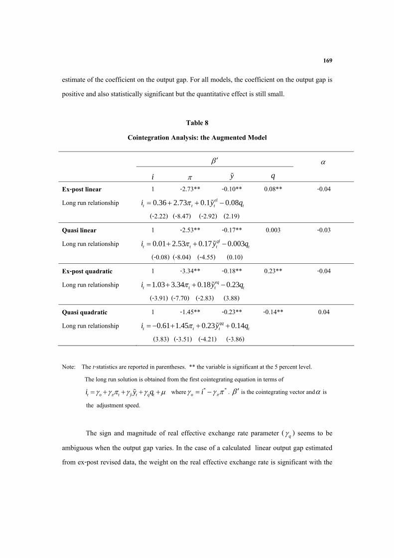
estimate of the coefficient on the output gap. For all models, the coefficient on the output gap is positive and also statistically significant but the quantitative effect is still small.

Table 8 Cointegration Analysis: the Augmented Model

i y q

Ex-post linear 1 -2.73** -0.10** 0.08** -0.04 Long run relationship 0.36 2.73 0.1 0.08el

t t t ti y q (-2.22) (-8.47) (-2.92) (2.19)

Quasi linear 1 -2.53** -0.17** 0.003 -0.03 Long run relationship 0.01 2.53 0.17 0.003ql

t t t ti y q (-0.08) (-8.04) (-4.55) (0.10)

Ex-post quadratic 1 -3.34** -0.18** 0.23** -0.04 Long run relationship 1.03 3.34 0.18 0.23eq

t t t ti y q (-3.91) (-7.70) (-2.83) (3.88)

Quasi quadratic 1 -1.45** -0.23** -0.14** 0.04 Long run relationship 0.61 1.45 0.23 0.14qq

t t t ti y q (3.83) (-3.51) (-4.21) (-3.86)

Note: The t-statistics are reported in parentheses. ** the variable is significant at the 5 percent level. The long run solution is obtained from the first cointegrating equation in terms of t o t y t q ti y q where * *

o i . is the cointegrating vector and is the adjustment speed.

The sign and magnitude of real effective exchange rate parameter ( q ) seems to be

ambiguous when the output gap varies. In the case of a calculated linear output gap estimated from ex-post revised data, the weight on the real effective exchange rate is significant with the

170

correct sign, whereas this weight is not significant when quasi-real time data is used. For cases where the output gap estimate is based on a quadratic time trend, q is always significant but provides the incorrect sign when the quasi-real time data is used. For all cases, the quantitative effect of the real effective exchange rate is small.

The adjustment speed parameters ( ) in the interest rate equation are greater than 0 in absolute term. This implies a stable model where deviations of the equilibrium value are corrected by monetary policy actions. The implied estimate of the long run nominal interest rate ( *i ) is either 5.13 or 4.43, in cases where the output gap is calculated with a linear trend based on ex-post and quasi-real time data, respectively, when calculating the output gap based on a quadratic trend based with either ex-post and quasi-real time data, we get calculated values for

*i is 6.87, 1.92, respectively. The results seem to be consistent with the baseline models. That is the linear trend provides values closer to the original Taylor (1993) model than the quadratic trend does.

Inflation and output gap parameters change when quasi-real time data are used to estimate the output gap instead of ex-post revised data. The inflation parameters become lower when quasi-real time data are used for both linear and quadratic time trends. But the output gap parameters become higher when quasi-real time data are used.

171

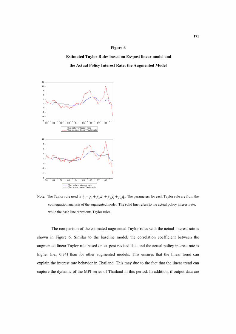
Figure 6 Estimated Taylor Rules based on Ex-post linear model and

the Actual Policy Interest Rate: the Augmented Model

-6

-4

-2

0

2

4

6

8

10

12

00 01 02 03 04 05 06 07 08

The policy interest rateThe ex-post linear Taylor rule

-6

-4

-2

0

2

4

6

8

10

00 01 02 03 04 05 06 07 08

The policy interest rateThe quasi linear Taylor rule

Note: The Taylor rule used is t o t y t q ti y q . The parameters for each Taylor rule are from the cointegration analysis of the augmented model. The solid line refers to the actual policy interest rate, while the dash line represents Taylor rules.

The comparison of the estimated augmented Taylor rules with the actual interest rate is

shown in Figure 6. Similar to the baseline model, the correlation coefficient between the augmented linear Taylor rule based on ex-post revised data and the actual policy interest rate is higher (i.e., 0.74) than for other augmented models. This ensures that the linear trend can explain the interest rate behavior in Thailand. This may due to the fact that the linear trend can capture the dynamic of the MPI series of Thailand in this period. In addition, if output data are

172

revised, the policy recommendations are also changed. 8 The implied Taylor rule paths associated with the quasi-real time data are consistently below those using ex-post revised in estimating the output gap.9

The conclusions that seem to be robust to choice of output gap proxy, from 2000 to 2009, is that the use of quasi-real time data does change the specification of the Taylor rules; some parameters change. Inflation and the real effective exchange rate parameters are especially especially sensitive to the use of the quadratic trend in calculating the output gap. In addition, the results suggest that a monetary policy rule which simultaneously includes inflation, the output gap and the real effective exchange rate may not be the best approximation to the process by which the interest rate is determined in Thailand. This may be due to the fact that the BOT was likely to target the price level directly rather than target inflation through current exchange rate.

6. Conclusions

This paper studies the process through which the interest rate is set in the Thai economy. Two main issues of monetary policy are emphasized. The first tries to test whether the interest rate set by the BOT has served as the nominal anchor of the Thai economy. The second aims to identify the targets of the monetary policy. In order to find out the solutions, we use a simple monetary policy rule suggested by the Taylor rule. Nevertheless, the Taylor rule is always constructed in the presence of the potential uncertainties. In general, the uncertainties in the potential output estimation are from three main sources. First of all, no central banks explicitly presume the definition of potential output they use, thus, several methods are proposed to estimate it. As different methods give us different potential output estimates, different policy decisions are suggested. We call this uncertainty the model uncertainty. The

8 Plots for the others are available in the full text version. 9 The Taylor rules with the quadratic trend are also consistent.

173

second uncertainty is the statistical uncertainty, which is concerned with the proper size of our sample in potential output estimation.

Finally, the output data that central bankers have access to are always revised before the final publication is shown. So it is not accurate to analyze the Taylor rule with ex-post revised data that central bankers did not have when making policy decisions. Consequently, the Taylor rule, which responds to the current output gap, becomes problematic in practice. This uncertainty is called the data uncertainty. However, this paper is concerned about the integration properties of the data. Thus, we allow the test for the possibility of cointegration among the nonstationary series to estimate the Taylor rule.

The cointegration analysis suggests that the interest rate has been strongly sensitive to inflation regardless of which output gap estimate is used. The so-called Taylor principle, moreover, holds in every rule calculated with different output gap estimates. The adjustment speed is greater than zero in all cases, which implies a stable model where deviations of the rate from its equilibrium value are corrected by monetary policy actions. As a result, the estimates from the cointegrating vector can be interpreted as a monetary policy reaction function.

The evidence shows that in the recent years monetary policy in Thailand, through its effect on interest rates, has performed the role of nominal anchor of the economy. This means that in the case of emerging market economy such as Thailand the fixed exchange rate regime is not the only option for a small open economy. However, the real effective exchange rate (REER) insignificantly enters to the model if the quasi-real time data are used in output gap estimation. Only when the Taylor rule is computed with quasi-real time data and the linear trend is used to estimate the output gap gives the expected signs, but the quantitative effect is small and insignificant. In other words, the augmented Taylor rules are affected by different output gap estimates. This may suggest that the Thai monetary policy was price stabilizing rather than exchange rate stabilizing in the period here considered. In other words, under the inflation targeting regime, inflation and the output gap can be considered as the main target variables rather than the REER.

174

In addition, this study finds that the Taylor rule with linear time trend output gap better explains observed interest rate behavior in Thailand then when we used the quadratic trend. This is beneficial for researchers analyzing the Thai economy, who need to consider carefully how they calculate output gaps.. For the influence of output data revision, which makes the choice between ex-post and quasi-real time data in estimating the output gap, the Taylor rules provide different policy recommendations for evaluating monetary policy in Thailand, especially in the crisis period. Hence, in practice, we should be prudent with the interpretation of the estimated Taylor rules, which is governed by the uncertainties due to the information problem. An extension of the our model and tests, using other potential output definitions, is an interesting topic for future research.

175

References

Books Ender, W. (1995). Applied Econometric Time Series.( 1st Edition) New York. John Wiley & Sons.

Greene, W. H. (2008). Econometric Analysis. (6th Edition) New Jersey: Prentice Hall.

Gujarati, D. N. (2003). Basic Econometrics. (4th Edition) Singapore: McGraw-Hill.

Articles Adema, Y (2004). A Taylor Rule for the Euro Area Based on Quasi-Real Time Data.

De Nederlandsche, Bank DNB Staff Reports, No. 114.

Andrade, J. & Divino, J.A (2005). Monetary policy of the Bank of Japan-inflation target versus exchange rate target. Japan and the world economy 17, 189-208.

Chai-anant, C., Pongsaparn, R. & Tansuwanarat, K (2008). Roles of Exchange Rate in Monetary Policy under Inflation Targeting: A Case Study for Thailand. Discussion paper BOT.

Christensen, A. M. & Nielsen, H. B (2003). Has US Monetary Policy followed the Taylor rule? A Cointegration Analysis 19988-2002. Mimeo.

Chuenchoksan, S., Nakornthab, D., & Tanboon, S (2008). Uncertainty in the Estimation of the Potential Output and Implications for the Conduct of Monetary Ploicy. BOT symposium.

Clarida, R., Jordi G., & Mark Gertler (1998). Monetary Policy Rules in practice Some international evidence. European Economic Review, 42(6), 1033-1067.

176

Eleftheriou, M (2009). Monetary policy in Germany: A cointegration analysis on the relevance of interest rate rules. Economic Modelling 26, 946-960.

Khemangkorn, V., Mallikamas, R. P. & Sutthasri, P (2008). Inflation Dynamics and Implications on Monetary Policy. BOT Symposium.

Kutter, Kenneth N. & Posen Adam S (2004). The difficulty of discerning what’s too tight: Taylor rules and Japanese monetary policy. North American Journal of Economics and Finance 15, 53–74.

McCallum, B., (2000). Alternative Monetary Policy Rules: A Comparison with Historical Settings for the United States, the United Kingdom, and Japan. Federal Reserve Bank of Richmond Economic Quarterly volume 86/1.

Ng, S. & Perron, P.(2001). Lag length selection and the construction of unit root test with good size and power. Econometrica 69, 1519-1554.

Orphanides, A. (1997). Monetary Policy Rules Based on Real-Time Data. American Economic Review 91, 964-985.

Orphanides, A. & van Nordan, S. (2002). The Unreliability of Output Gap Estimates in Real Time. Review of Economics and Statistics 84, 569-583.

Osterholm, P. (2005). The Taylor rule: a spurious regression? Bulletin of Economic Research 57 (3), 217-247.

Taylor, John B. (1993). Discretion versus Policy Rules in Practice. Carnegie-Rochester Conference Series on Public Policy 39: 195–214.

Torres, Alberto (2003). Monetary policy and interest rates: evidence from Mexico. The North American Journal of Economics and Finance. 14, 257-379.

177

Other materials Sinthuprasirt, S. (2002). The Test of Taylor rule on Thai monetary policy. Faculty of

Economics, Chulalongkorn University. (In Thai).

Punjataewakupt, P.(2009). Response of Core inflation to Economics variables: After Adopting Inflation Target. Faculty of Economics, Thammasat University.(In Thai).

178

Appendix

1. The Fitted Linear Trend

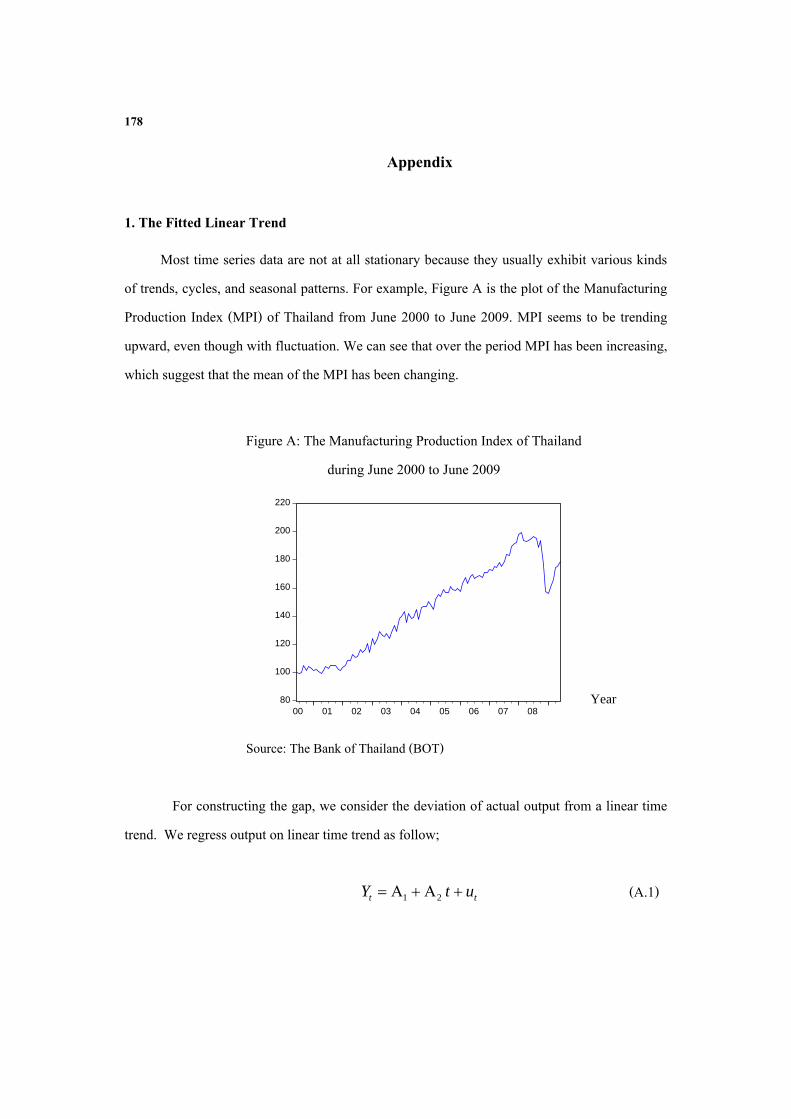
Most time series data are not at all stationary because they usually exhibit various kinds of trends, cycles, and seasonal patterns. For example, Figure A is the plot of the Manufacturing Production Index (MPI) of Thailand from June 2000 to June 2009. MPI seems to be trending upward, even though with fluctuation. We can see that over the period MPI has been increasing, which suggest that the mean of the MPI has been changing.

Figure A: The Manufacturing Production Index of Thailand

during June 2000 to June 2009

80

100

120

140

160

180

200

220

00 01 02 03 04 05 06 07 08

Source: The Bank of Thailand (BOT)

For constructing the gap, we consider the deviation of actual output from a linear time

trend. We regress output on linear time trend as follow;

tt utY 21 (A.1)

Year

179

where t is the time index or the trend variable measured chronologically. The parameters 1 and 2 (the "intercept" and "slope" of the trend line) are usually estimated via a simple regression in which tY is the dependent variable and the time index t is the independent variable. This procedure of removing the trend is called detrending. And the residual from the regression is

ˆˆt t tu Y Y (A.2)

tu is known as a linearly detrended time series which is the output gap ( i.e. tY is assumed to be the potential ). 2. The Fitted Quadratic Trend

Instead of linear trend, we regress the output on a constant, time and time squared.

tt uttY 2

321 (A.3) The residuals from Eq. (A.3) are quadratically detrended time series. Similarly, the output gap is the residuals from this regression ( tu ).