TRITA-MMK 2000:16ISSN 1400-1179

ISRN KTH/MMK/R--00/16--SEMRTC Report 00/15

V 1.01

Monitoring, Testing and Debugging ofDistributed Real-Time Systems

byHenrik Thane

Stockholm 2000Doctoral Thesis

Mechatronics Laboratory,Department of Machine Design

Royal Institute of Technology, KTHS-100 44 Stockholm,

Sweden

Akademisk avhandling som med tillstånd från Kungliga Tekniska Högskolan iStockholm, framlägges till offentlig granskning för avläggande av teknologiedoktorsexamen fredagen den 26 maj 2000 kl. 10.00 i sal M2, Kungliga TekniskaHögskolan, Brinellvägen 64, Stockholm.

Fakultetsopponent: Jan Jonsson, Chalmers Tekniska Högskola, Göteborg.

© Henrik Thane 2000

Mälardalen Real-Time Research Centre (MRTC),Department of Computer EngineeringMälardalen University (MDH)S-721 23 Västerås

(www.mrtc.mdh.se, henrik.thane@mdh.se)

ToMarianne and Cornelia

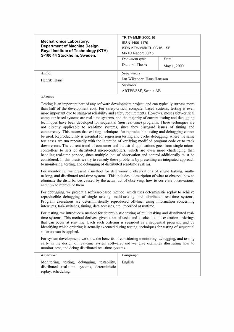
TRITA-MMK 2000:16ISSN 1400-1179ISRN KTH/MMK/R--00/16—SEMRTC Report 00/15

Mechatronics Laboratory,Department of Machine DesignRoyal Institute of Technology (KTH)S-100 44 Stockholm, Sweden.

Document typeDoctoral Thesis

Date

May 1, 2000

SupervisorsJan Wikander, Hans Hansson

Author

Henrik ThaneSponsorsARTES/SSF, Scania AB

Abstract

Testing is an important part of any software development project, and can typically surpass morethan half of the development cost. For safety-critical computer based systems, testing is evenmore important due to stringent reliability and safety requirements. However, most safety-criticalcomputer based systems are real-time systems, and the majority of current testing and debuggingtechniques have been developed for sequential (non real-time) programs. These techniques arenot directly applicable to real-time systems, since they disregard issues of timing andconcurrency. This means that existing techniques for reproducible testing and debugging cannotbe used. Reproducibility is essential for regression testing and cyclic debugging, where the sametest cases are run repeatedly with the intention of verifying modified program code or to trackdown errors. The current trend of consumer and industrial applications goes from single micro-controllers to sets of distributed micro-controllers, which are even more challenging thanhandling real-time per-see, since multiple loci of observation and control additionally must beconsidered. In this thesis we try to remedy these problems by presenting an integrated approachto monitoring, testing, and debugging of distributed real-time systems.

For monitoring, we present a method for deterministic observations of single tasking, multi-tasking, and distributed real-time systems. This includes a description of what to observe, how toeliminate the disturbances caused by the actual act of observing, how to correlate observations,and how to reproduce them.

For debugging, we present a software-based method, which uses deterministic replay to achievereproducible debugging of single tasking, multi-tasking, and distributed real-time systems.Program executions are deterministically reproduced off-line, using information concerninginterrupts, task-switches, timing, data accesses, etc., recorded at runtime.

For testing, we introduce a method for deterministic testing of multitasking and distributed real-time systems. This method derives, given a set of tasks and a schedule, all execution orderingsthat can occur at run-time. Each such ordering is regarded as a sequential program, and byidentifying which ordering is actually executed during testing, techniques for testing of sequentialsoftware can be applied.

For system development, we show the benefits of considering monitoring, debugging, and testingearly in the design of real-time system software, and we give examples illustrating how tomonitor, test, and debug distributed real-time systems.

Keywords

Monitoring, testing, debugging, testability,distributed real-time systems, deterministicreplay, scheduling.

Language

English

2

3

Preface

Science and technology have fascinated me as long as I can remember. When I was akid, comics, TV-shows, popular science magazines, movies, school, and sciencefiction books set off my imagination.

When I was a teenager, computers started to fascinate me, and I started to playaround with games programming, which proved to be a very creative, intellectuallystimulating, and fun activity. This experience went on for years and made me realizethat computers and computer programming were things I really wanted to work within the future.

And, so it became. Parallel with studies at the university, I worked part time as acomputer programmer for a company that designed real-time system applications,and I kept at it for a year after graduation. After some escapades around the world, Ibegan studying for a Ph.D. at the Royal Institute of Technology (KTH), in April1995. My research topic was safe and reliable software in embedded real-time systemapplications. This resulted in a Licentiate degree in Mechatronics, in the fall of 1997.The research topic was a bit broad, but gave me great insight into the problems ofdesigning and verifying safe and reliable computer software. While still beingassociated with the Mechatronics laboratory at the KTH, I moved in the fall of 1997to Mälardalen University in Västerås, and started working as part time teacher andpart time Ph.D. student. At the same time my research narrowed and I begun focusingon testability of real-time systems, which for natural reasons led me to also considertesting, debugging and monitoring. That work gave fruit – this thesis.

The work presented in this thesis would not have been possible if I had not had suchstimulating and creative people around me, including my supervisors Jan Wikanderand Hans Hansson. I am also very grateful for the financial support provided by thenational Swedish Real-Time Systems research initiative, ARTES, supported by theSwedish Foundation for Strategic Research, as well as for the donation provided byScania AB during 1995-1997.

However, my greatest thanks go Hans Hansson, Christer Norström, KristianSandström, and Jukka-Mäki Turja for all creative work, and intense, and stimulatingdiscussions we have had during the years. Other special thanks go to Anders Wall,Mårten Larsson, Gerhard Fohler, Mohammed El-Shobaki, Markus Lindgren, BjörnAlvin, Sasikumar Punnekkat, Iain Bate, Mikael Sjödin, Mikael Gustafsson andMartin Törngren for also providing insightful input. Not only being a friendly bunchof people, they have all also over the years provided input and feedback on drafts ofpapers – not forgetting, this thesis. Thank you very much.

A very special thank you goes to Harriet Ekwall for handling all the ground servicehere at MRTC, and for always being such happy and friendly spirit. Thank you.

Finally, the greatest debt I owe to my family, Marianne and Cornelia, who have beenextremely supportive, not to mention Cornelia’s artwork on my thesis drafts.

Västerås, a beautiful and warm spring day in April 2000.

4

5

Publications

1. Thane H and Hansson H. Testing Distributed Real-Time Systems. Submitted for journalpublication.

2. Thane H. and Hansson H. Using Deterministic Replay for Debugging of Distributed Real-TimeSystems. In proceedings of the 12th Euromicro Conference on Real-Time Systems (ECRTS’00),Stockholm, June 2000.

3. Thane H. Asterix the T-REX among real-time kernels. Timely, reliable, efficient and extraordinary.Technical report. In preparation. Mälardalen Real-Time Research Centre, Mälardalen University,May 2000.

4. Thane H, and Wall A. Formal and Probabilistic Arguments for Reuse and testing of Componentsin Safety-Critical Real-Time Systems. Technical report. Mälardalen Real-Time Research Centre,Mälardalen University, March 2000.

5. Thane H. and Hansson H. Handling Interrupts in Testing of Distributed Real-Time Systems. Inproc. Real-Time Computing Systems and Applications conference (RTCSA’99), Hong Kong,December 1999.

6. Thane H. and Hansson H. Towards Systematic Testing of Distributed Real-Time Systems. Inproceedings of the 20th IEEE Real-Time Systems Symposium (RTSS’99), Phoenix, Arizona,December 1999.

7. Thane H. Design for Deterministic Monitoring of Distributed Real-Time Systems. Technical report,Mälardalen Real-Time Research Centre, Mälardalen University, November 1999.

8. Norström C., Sandström K., Mäki-Turja J., Hansson H., and Thane H. Robusta Realtidssytem.Book. MRTC Press, September, 1999.

9. Thane H. and Hansson H. Towards Deterministic Testing of Distributed Real-Time Systems. InSwedish National Real-Time Conference SNART'99, August 1999.

10. Thane H. Safety and Reliability of Software in Embedded Control Systems. Licentiate thesis.TRITA-MMK 1997:17, ISSN 1400-1179, ISRN KTH/MMK/R--97/17--SE. MechatronicsLaboratory, the Royal Institute of Technology, S-100 44 Stockholm, Sweden, October 1997.

11. Thane H. and Norström C. The Testability of Safety-Critical Real-Time Systems. Technical report.Dept. computer engineering, Mälardalen University, September 1997.

12. Thane H. Safe and Reliable Computer Control Systems - an Overview. In proceedings of the 16th

Int. Conference on Computer Safety, Reliability and Security (SAFECOMP’97), York, UK,September 1997.

13. Thane H. and Larsson M. Scheduling Using Constraint Programming. Technical report. Dept.computer engineering, Mälardalen University, June 1997.

14. Thane H. and Larsson M. The Arbitrary Complexity of Software. Research Report. MechatronicsLaboratory, the Royal Institute of Technology, S-100 44 Stockholm, Sweden, May 1997.

15. Eriksson C., Thane H. and Gustafsson M. A Communication Protocol for Hard and Soft Real-TimeSystems. In the proceedings of the 8th Euromicro Real-Time Workshop, L'Aquila Italy, June 1996.

16. Thane, H. Safe and Reliable Computer Control Systems - Concepts and Methods. Research ReportTRITA-MMK 1996:13, ISSN 1400-1179, ISRN KTH/MMK/R-96/13-SE. MechatronicsLaboratory, the Royal Institute of Technology, S-100 44 Stockholm, Sweden, 1996.

17. Eriksson C., Gustafsson M., Gustafsson J., Mäki-Turja J., Thane H., Sandström K., and Brorson E.Real-TimeTalk a Framework for Object-Oriented Hard & Soft Real-Time Systems. In proceedingsof Workshop 18: Object-Oriented Real-Time Systems at OOPSLA,Texas,USA,October 1995.

6

7

Contents

1 INTRODUCTION...........................................................................................................................9

2 BACKGROUND ...........................................................................................................................11

2.1 THE SCENE...............................................................................................................................112.2 COMPLEXITY............................................................................................................................112.3 SAFETY MARGINS.....................................................................................................................12

2.3.1 Robust designs ................................................................................................................122.3.2 Redundancy.....................................................................................................................13

2.4 THE VERIFICATION PROBLEM ...................................................................................................142.4.1 Testing.............................................................................................................................142.4.2 Removing errors..............................................................................................................152.4.3 Formal methods ..............................................................................................................15

2.5 TESTABILITY............................................................................................................................162.5.1 Ambition and effort .........................................................................................................182.5.2 Why is high testability a necessary quality? ...................................................................20

2.6 SUMMARY................................................................................................................................21

3 THE SYSTEM MODEL AND TERMINOLOGY .....................................................................23

3.1 THE SYSTEM MODEL................................................................................................................233.2 TERMINOLOGY.........................................................................................................................23

3.2.1 Failures, failure modes, failure semantics, and hypotheses............................................233.2.2 Determinism and reproducibility ....................................................................................28

4 MONITORING DISTRIBUTED REAL-TIME SYSTEMS .....................................................31

4.1 MONITORING............................................................................................................................354.2 HOW TO COLLECT SUFFICIENT INFORMATION ...........................................................................364.3 ELIMINATION OF PERTURBATIONS ............................................................................................38

4.3.1 Hardware monitoring .....................................................................................................384.3.2 Hybrid monitoring...........................................................................................................394.3.3 Software monitoring........................................................................................................40

4.4 DEFINING A GLOBAL STATE ......................................................................................................434.5 REPRODUCTION OF OBSERVATIONS..........................................................................................44

4.5.1 Reproducing inputs .........................................................................................................444.5.2 Reproduction of complete system behavior.....................................................................45

4.6 SUMMARY................................................................................................................................45

5 DEBUGGING DISTRIBUTED REAL-TIME SYSTEMS ........................................................47

5.1 THE SYSTEM MODEL ................................................................................................................495.2 REAL-TIME SYSTEMS DEBUGGING ............................................................................................50

5.2.1 Debugging single task real-time systems ........................................................................505.2.2 Debugging multitasking real-time systems......................................................................505.2.3 Debugging distributed real-time systems........................................................................52

5.3 A SMALL EXAMPLE ..................................................................................................................535.4 DISCUSSION .............................................................................................................................545.5 RELATED WORK .......................................................................................................................565.6 SUMMARY................................................................................................................................57

6 TESTING DISTRIBUTED REAL-TIME SYSTEMS ...............................................................59

6.1 THE SYSTEM MODEL ................................................................................................................626.2 EXECUTION ORDER ANALYSIS ..................................................................................................63

6.2.1 Execution Orderings .......................................................................................................636.2.2 Calculating EXo(J) ..........................................................................................................65

6.3 THE EOG ALGORITHM .............................................................................................................69

8

6.3.1 GEXo – the Global EOG .................................................................................................716.4 TOWARDS SYSTEMATIC TESTING..............................................................................................76

6.4.1 Assumptions ....................................................................................................................766.4.2 Test Strategy....................................................................................................................776.4.3 Coverage .........................................................................................................................776.4.4 Reproducibility................................................................................................................79

6.5 EXTENDING ANALYSIS WITH INTERRUPTS.................................................................................806.6 OTHER ISSUES..........................................................................................................................82

6.6.1 Jitter ................................................................................................................................826.6.2 Start times and completion times ....................................................................................836.6.3 Testability........................................................................................................................836.6.4 Complexity ......................................................................................................................83

6.7 SUMMARY................................................................................................................................85

7 CASE STUDY ...............................................................................................................................87

7.1 A DISTRIBUTED CONTROL SYSTEM...........................................................................................877.2 ADDING PROBES FOR OBSERVATION.........................................................................................907.3 GLOBAL EXECUTION ORDERINGS .............................................................................................937.4 GLOBAL EXECUTION ORDERING DATA DEPENDENCY TRANSFORMATION..................................947.5 TESTING...................................................................................................................................947.6 IMPROVING TESTABILITY..........................................................................................................967.7 SUMMARY................................................................................................................................97

8 THE TESTABILITY OF DISTRIBUTED REAL-TIME SYSTEMS ......................................99

8.1 OBSERVABILITY.......................................................................................................................998.2 COVERAGE.............................................................................................................................1008.3 CONTROLLABILITY.................................................................................................................1008.4 TESTABILITY..........................................................................................................................101

9 CONCLUSIONS .........................................................................................................................103

10 FUTURE WORK ....................................................................................................................105

10.1 MONITORING, TESTING AND DEBUGGING ...............................................................................10510.2 FORMAL AND PROBABILISTIC ARGUMENTS FOR COMPONENT REUSE AND TESTING IN SAFETY-CRITICAL REAL-TIME SYSTEMS...........................................................................................................106

10.2.1 Software components in real-time systems?..................................................................10710.2.2 Component contracts ....................................................................................................10810.2.3 Component contract analysis........................................................................................11210.2.4 Summary .......................................................................................................................117

11 REFERENCES........................................................................................................................119

9

1 INTRODUCTIONThe introduction of computers into safety-critical systems lays a heavy burden onsoftware designers. Public and legislators demand reliable and safe computersystems, equal to or better than the mechanical or electromechanical parts theyreplace. The designers must have a thorough understanding of the system and moreaccurate software design and verification techniques than have usually been deemednecessary for software development. However, since computer related problems,relating to safety and reliability, have just recently been of any concern for engineers,there are no holistic engineering principles for construction of safe and reliablecomputer based systems. There exist only scarce pools of knowledge and no silverbullets1 that can handle everything. Some people do nonetheless, with an almostreligious glee, decree that their method, principle or programming language handlesor kills all werewolves (which these days have shrunken to tiny, but sometimes lethalbugs) [9][38][85].

The motivation for writing this thesis is an ambition to increase the depth ofknowledge in the pool of distributed real-time systems verification, which previouslyhas been very shallow. We will specifically address testing and debugging, and asmost real-time systems are embedded with limited observability, we will also covermonitoring. Testing is an important part of any software development project, andcan typically surpass more than half of the development cost. High testability istherefore of significance for cost reduction, but also for the ability to reach thereliability levels required for safety-critical systems. A significant part of this thesisis accordingly dedicated to discussions on testability, and testability increasingmeasures for distributed real-time systems.

The shallowness of knowledge in the pool of distributed real-time systemsverification, is partly due to the fact that the majority of current testing anddebugging techniques have been developed for sequential programs. Thesetechniques are as such not directly applicable to real-time systems since theydisregard timing and concurrency issues. The implication is that reproducible testingand debugging are not possible using these techniques. Reproducibility is essentialfor regression testing and cyclic debugging, where the same test cases are runrepeatedly with the intention of verifying modified program code or to track downerrors (bugs). The current trend of consumer and industrial applications goes fromsingle micro-controllers to sets of distributed micro-controllers, for which currenttesting and debugging techniques also are insufficient; they cannot handle themultiple loci of observation and control required. In this thesis we try to remedythese problems by presenting novel approaches to monitoring, testing, and debuggingof both single CPU and distributed real-time systems.

The main contributions of this thesis are in the fields of:

• Monitoring. We present a method for deterministic observations of singletasking, multi-tasking, and distributed real-time systems. This includes adescription of what to observe, how to eliminate the disturbances caused by theactual act of observing, how to correlate observations between nodes, and how toreproduce the observations. We will give a taxonomy of different observationtechniques, and discuss where, how and when these techniques should be appliedfor deterministic observations. We argue that it is essential to consider

1 Silver bullets, which in folklore are the only means to slay the mythical werewolves.

10

monitoring early in the design process, in order to achieve efficient anddeterministic observations.

• Debugging. We present a software based technique for achieving reproducibledebugging of single tasking, multi-tasking, and distributed real-time systems, bymeans of deterministic replay. During runtime, information is recorded withrespect to interrupts, task-switches, timing, and data. The system behavior canthen be deterministically reproduced off-line using the recorded information. Astandard debugger can be used without the risk of introducing temporal sideeffects, and we can reproduce interrupts, and task-switches with a timingprecision corresponding to the exact machine instruction at which they occurred.The technique also scales to distributed real-time systems, so that reproducibledebugging, ranging from one node at a time, to multiple nodes concurrently, canbe performed.

• Testing. We present a method for deterministic testing of multitasking real-timesystems, which allows explorative investigations of real-time system behavior.For testing of sequential software it is usually sufficient to provide the sameinput (and state) in order to reproduce the output. However, for real-time systemsit is not sufficient to provide the same inputs for reproducibility – we need also tocontrol, or observe, the timing and order of the inputs and the concurrency of theexecuting tasks. The method includes an analysis technique that given a set oftasks and a schedule derives all execution orderings that can occur during run-time. The method also includes a testing strategy that using the derived executionorderings can achieve deterministic, and even reproducible, testing of real-timesystems. Each execution ordering can be regarded as a sequential program andthus techniques used for testing of sequential software can be applied to real-timesystem software. We also show how this analysis and testing strategy can beextended to encompass interrupt interference, distributed computations,communication latencies and the effects of global clock synchronization. Thenumber of execution orderings is an objective measure of the testability of asystem since it indicates how many behaviors the system can exhibit duringruntime. In the pursuit of finding errors we must thus cover all these executionorderings. The fewer the orderings the better the testability.

Outline:

The outline of this thesis is such that we begin in chapter 2 with a description of thepeculiarities of software in general and why software verification constitutes such asignificant part of any software development project. In chapter 3, we define a basicsystem model and some basic terminology, which we will refine further on in thethesis. In chapter 4, we give an introduction to monitoring of real-time systems(RTS), and discuss and give solutions on how monitoring can be deterministicallyachieved in RTS, and distributed real-time systems (DRTS). In chapter 5, we discussand present some solutions to deterministic and reproducible debugging of DRTS. Inchapter 6, we present our approach to deterministic testing of DRTS, includingresults on how to measure the testability of RTS, and DRTS. In chapter 7, we presenta larger example illustrating the use of the techniques presented in chapters 3, and 5.In chapter 8, we discuss the testability of DRTS. Finally, in chapter 9 we summarizeand draw some conclusions, and in chapter 10 we outline some future work.

11

2 BACKGROUNDThis thesis is about monitoring, testing, and debugging, of distributed real-timesystems, but as a background and to set the scene we begin with a description ofthe peculiarities pertaining to computer software development and why softwareverification is such a dominant factor in the development process.

2.1 The sceneExperience with software development has shown that software is often deliveredlate, over budget, and despite all that still functionally incorrect. A question isoften asked: ”What is so different about software engineering? Why do notsoftware engineers do it right, like traditional engineers? Or at least once in awhile?”

These unfavorable questions are not uncalled for; the traditional engineeringdisciplines are founded on science and mathematics and are able to model andpredict the behavior of their designs. Software engineering is more of a craft,based on trial and error, rather than on calculation and prediction. However,knowing the peculiarities of software, this comparison is not entirely fair; it doesnot acknowledge that computers and software differ from physical systems ontwo key accounts:

(1) They have discontinuous behavior and

(2) Software lacks physical attributes like e.g., mass, inertia, size, and lacksstructure or function related attributes like e.g., strength, density and form.

The sole physical attribute that can be modeled and measured by softwareengineers is time. Therefore, there exist sound work and theories regardingmodeling and verification of systems’ temporal attributes [4][75][117][58]. Thetheory for real-time systems gives us a platform for more “engineering wise”modeling and verification of computer software, but since the theory is mostlyconcerned with timing, and ordering of events, we still have to face functionalverification.

We will now in the remainder of this chapter discuss the peculiarities of softwaredevelopment compared to classical engineering. We will discuss the impact thatthe two fundamental differences (1 and 2 above) have on software developmentas compared to classical engineering of physical systems. We will progress inseveral steps: beginning with software complexity, and then continuing on withsafety margins, testing, modeling, validation, and finally testability.

2.2 ComplexityThe two properties (1) and (2) above give rise to both advantages anddisadvantages compared to regular physical systems. One good thing is thatsoftware is easy to change and mutate hence the name software. The bad thing isthat complexity easily arises. Having no physical limitations, complex softwaredesigns are possible and no real effort to accomplish this complexity is needed.That is, it is very easy to produce solutions to a problem that are vastly morecomplex than the intrinsic complexity of the problem.

12

Complexity is a source of design faults. Design faults are often due to failure toanticipate certain interactions between components in the system. As complexityincreases, design faults are more prone to occur since more interactions make itharder to identify all possible behaviors. Since, software does not suffer fromgravity, or have any limits to structural strength there is nothing that hinders ourimagination in solving problems using software. Although not explicitlyexpressed, programming languages, programming methodologies and processesin fact introduces virtual physical laws and restrains the imagination of theprogrammers. At a seminar Nobel Prize winner Richard Feynman once said:“Science is imagination in a straightjacket.”

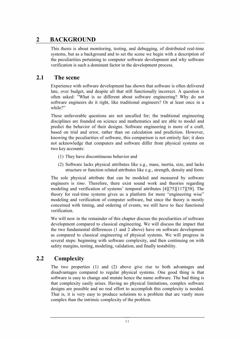
2.3 Safety marginsIn the classical engineering disciplines such as civilengineering it is common practice to make use of safetymargins. Bridges are, for example, often designed towithstand loads far greater than they would encounterduring normal use. For software it is in the classicalsense not possible to directly make use of safety marginsbecause software is pure design – like the blue prints forbridges. Safety margins on software would be likesubstituting the paper in the blue prints for thick sheets of steel. Software is puredesign and can thus not be worn-out or broken by physical means. The physicalmemory where the software resides can of course be corrupted due to physicalfailures (often transient), but not the actual software. All system failures due toerrors in the software are design-flaws, built into the system from the beginning(Figure 2-1).

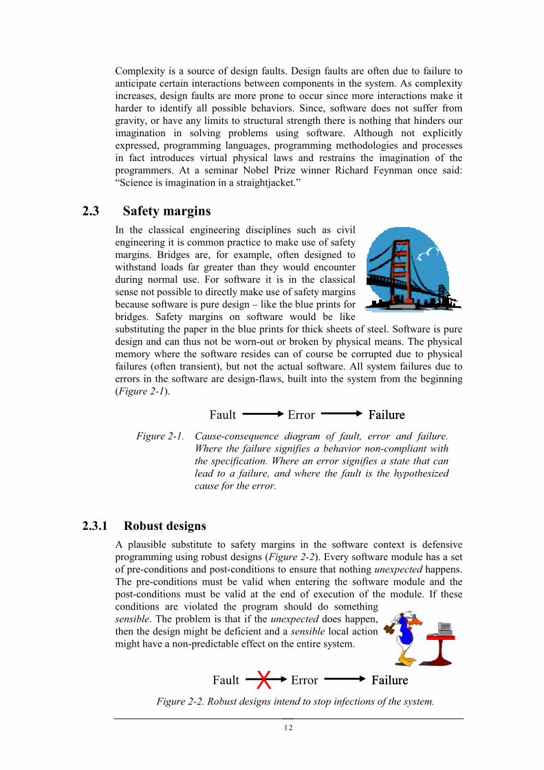
2.3.1 Robust designsA plausible substitute to safety margins in the software context is defensiveprogramming using robust designs (Figure 2-2). Every software module has a setof pre-conditions and post-conditions to ensure that nothing unexpected happens.The pre-conditions must be valid when entering the software module and thepost-conditions must be valid at the end of execution of the module. If theseconditions are violated the program should do somethingsensible. The problem is that if the unexpected does happen,then the design might be deficient and a sensible local actionmight have a non-predictable effect on the entire system.

Fault Error FailureFailureFigure 2-1. Cause-consequence diagram of fault, error and failure.

Where the failure signifies a behavior non-compliant withthe specification. Where an error signifies a state that canlead to a failure, and where the fault is the hypothesizedcause for the error.

Fault Error FailureFailureFigure 2-2. Robust designs intend to stop infections of the system.

13

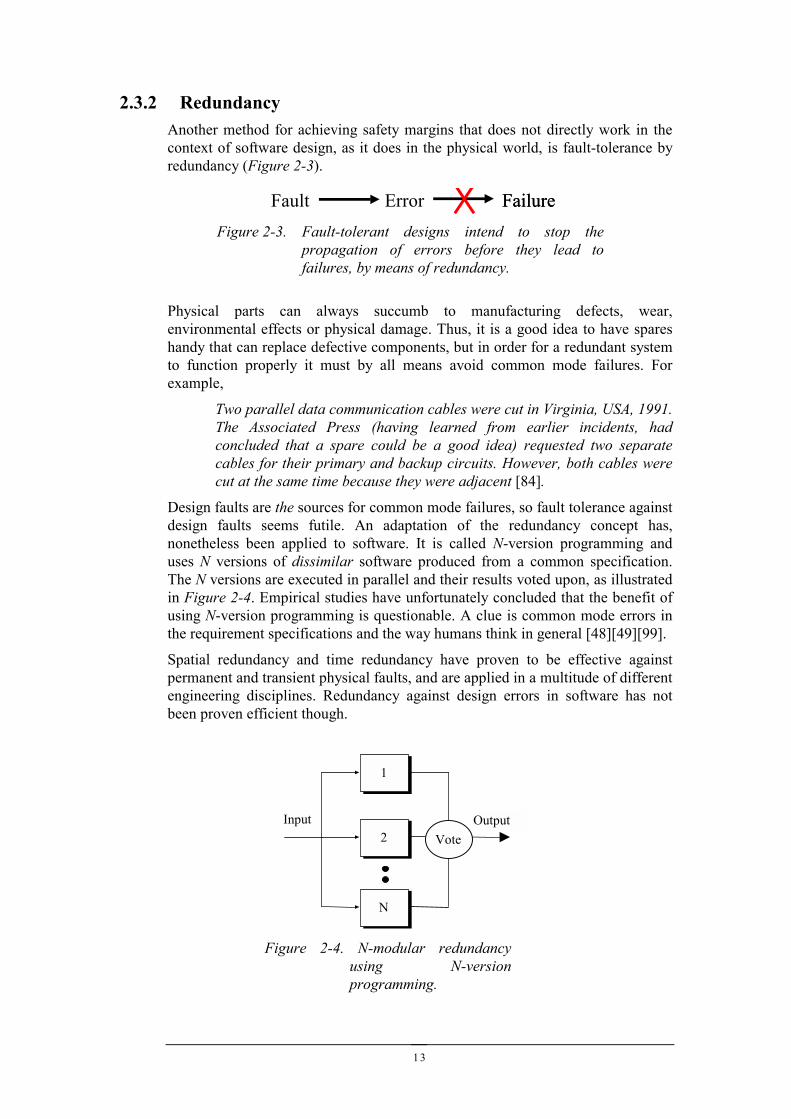
2.3.2 RedundancyAnother method for achieving safety margins that does not directly work in thecontext of software design, as it does in the physical world, is fault-tolerance byredundancy (Figure 2-3).

Physical parts can always succumb to manufacturing defects, wear,environmental effects or physical damage. Thus, it is a good idea to have spareshandy that can replace defective components, but in order for a redundant systemto function properly it must by all means avoid common mode failures. Forexample,

Two parallel data communication cables were cut in Virginia, USA, 1991.The Associated Press (having learned from earlier incidents, hadconcluded that a spare could be a good idea) requested two separatecables for their primary and backup circuits. However, both cables werecut at the same time because they were adjacent [84].

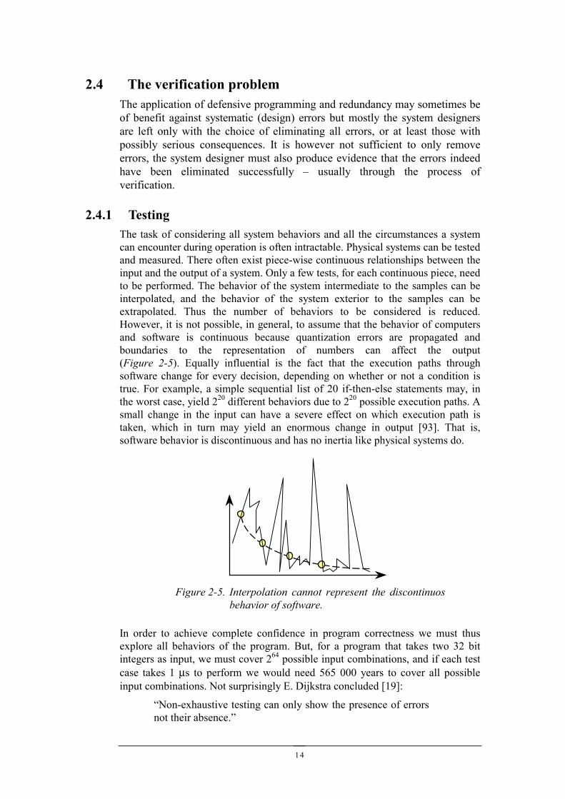
Design faults are the sources for common mode failures, so fault tolerance againstdesign faults seems futile. An adaptation of the redundancy concept has,nonetheless been applied to software. It is called N-version programming anduses N versions of dissimilar software produced from a common specification.The N versions are executed in parallel and their results voted upon, as illustratedin Figure 2-4. Empirical studies have unfortunately concluded that the benefit ofusing N-version programming is questionable. A clue is common mode errors inthe requirement specifications and the way humans think in general [48][49][99].

Spatial redundancy and time redundancy have proven to be effective againstpermanent and transient physical faults, and are applied in a multitude of differentengineering disciplines. Redundancy against design errors in software has notbeen proven efficient though.

Fault Error FailureFailureFigure 2-3. Fault-tolerant designs intend to stop the

propagation of errors before they lead tofailures, by means of redundancy.

Figure 2-4. N-modular redundancyusing N-versionprogramming.

Input Output2

N

1

Vote

14

2.4 The verification problemThe application of defensive programming and redundancy may sometimes beof benefit against systematic (design) errors but mostly the system designersare left only with the choice of eliminating all errors, or at least those withpossibly serious consequences. It is however not sufficient to only removeerrors, the system designer must also produce evidence that the errors indeedhave been eliminated successfully – usually through the process ofverification.

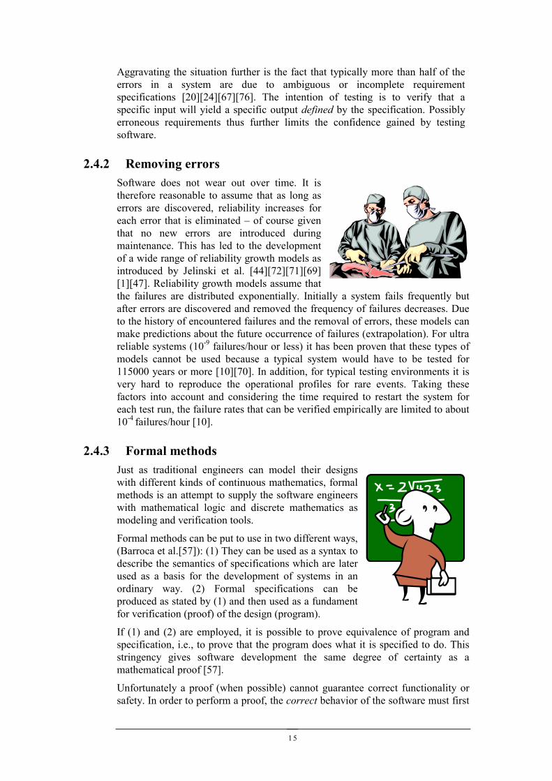
2.4.1 TestingThe task of considering all system behaviors and all the circumstances a systemcan encounter during operation is often intractable. Physical systems can be testedand measured. There often exist piece-wise continuous relationships between theinput and the output of a system. Only a few tests, for each continuous piece, needto be performed. The behavior of the system intermediate to the samples can beinterpolated, and the behavior of the system exterior to the samples can beextrapolated. Thus the number of behaviors to be considered is reduced.However, it is not possible, in general, to assume that the behavior of computersand software is continuous because quantization errors are propagated andboundaries to the representation of numbers can affect the output(Figure 2-5). Equally influential is the fact that the execution paths throughsoftware change for every decision, depending on whether or not a condition istrue. For example, a simple sequential list of 20 if-then-else statements may, inthe worst case, yield 220 different behaviors due to 220 possible execution paths. Asmall change in the input can have a severe effect on which execution path istaken, which in turn may yield an enormous change in output [93]. That is,software behavior is discontinuous and has no inertia like physical systems do.

In order to achieve complete confidence in program correctness we must thusexplore all behaviors of the program. But, for a program that takes two 32 bitintegers as input, we must cover 264 possible input combinations, and if each testcase takes 1 µs to perform we would need 565 000 years to cover all possibleinput combinations. Not surprisingly E. Dijkstra concluded [19]:

“Non-exhaustive testing can only show the presence of errorsnot their absence.”

Figure 2-5. Interpolation cannot represent the discontinuosbehavior of software.

15

Aggravating the situation further is the fact that typically more than half of theerrors in a system are due to ambiguous or incomplete requirementspecifications [20][24][67][76]. The intention of testing is to verify that aspecific input will yield a specific output defined by the specification. Possiblyerroneous requirements thus further limits the confidence gained by testingsoftware.

2.4.2 Removing errorsSoftware does not wear out over time. It istherefore reasonable to assume that as long aserrors are discovered, reliability increases foreach error that is eliminated – of course giventhat no new errors are introduced duringmaintenance. This has led to the developmentof a wide range of reliability growth models asintroduced by Jelinski et al. [44][72][71][69][1][47]. Reliability growth models assume thatthe failures are distributed exponentially. Initially a system fails frequently butafter errors are discovered and removed the frequency of failures decreases. Dueto the history of encountered failures and the removal of errors, these models canmake predictions about the future occurrence of failures (extrapolation). For ultrareliable systems (10-9 failures/hour or less) it has been proven that these types ofmodels cannot be used because a typical system would have to be tested for115000 years or more [10][70]. In addition, for typical testing environments it isvery hard to reproduce the operational profiles for rare events. Taking thesefactors into account and considering the time required to restart the system foreach test run, the failure rates that can be verified empirically are limited to about10-4 failures/hour [10].

2.4.3 Formal methodsJust as traditional engineers can model their designswith different kinds of continuous mathematics, formalmethods is an attempt to supply the software engineerswith mathematical logic and discrete mathematics asmodeling and verification tools.

Formal methods can be put to use in two different ways,(Barroca et al.[57]): (1) They can be used as a syntax todescribe the semantics of specifications which are laterused as a basis for the development of systems in anordinary way. (2) Formal specifications can beproduced as stated by (1) and then used as a fundamentfor verification (proof) of the design (program).

If (1) and (2) are employed, it is possible to prove equivalence of program andspecification, i.e., to prove that the program does what it is specified to do. Thisstringency gives software development the same degree of certainty as amathematical proof [57].

Unfortunately a proof (when possible) cannot guarantee correct functionality orsafety. In order to perform a proof, the correct behavior of the software must first

16

be specified in a formal, mathematical language. The task of specifying thecorrect behavior can be as difficult and error-prone as writing the software tobegin with [67][68]. In essence the difficulty comes from the fact that we cannotknow if we have accurately modeled the ”real system”, so we can never be certainthat the specification is complete. This distinction between model and realityattends all applications of mathematics in engineering. For example, the”correctness” of a control loop calculation for a robot depends on the fidelity ofthe control loop’s dynamics to the real behavior of the robot, on the accuracy ofthe stated requirements, and on the extent to which the calculations are performedwithout error.

These limitations are however, minimized in engineering by empirical validation.Aeronautical engineers believe that fluid dynamics accurately models the airflowing over the wing of an airplane, and civil engineers believe that structuralcalculus accurately models the structural integrity of constructions. Aeronauticalengineers and civil engineers have great confidence in their respective modelssince they have been validated in practice many times. Validation is an empiricalpursuit to test that a model accurately describes the real world.

Worth noting is that the validation of the formal models has to be done by testing,and as formal models are based on discrete mathematics they are discontinuous.The implication is thus that we cannot use interpolation or extrapolation, leavingus in the same position – again, as when using simple testing. We havenonetheless gained something compared to just applying testing solely; we canassume that the specifications are non-ambiguous and complete withinthemselves. Although, they may still be incomplete or erroneous with respect tothe real target system they attempt to model.

Further limitations to current formal methods are their lack of scalability (due toexponential complexity growth), and their inability to handle timing and resourceinadequacies, like violation of deadlines and overload situations (although sometools do handle time [60]). That is, any behavior (like overload) not described inthe formal model cannot be explored. Testing can however do just that, becausetesting explores the real system, not an abstraction.

2.5 TestabilitySo, even if we make use of formal methods and fault-tolerance we can nevereliminate testing completely. But, in order to achieve complete confidence in thecorrectness of software we must explore all possible behaviors, and from theabove discussion we can conclude that this is seemingly an impossible task.

A constructive approach to this situation has led to research into something calledtestability. It is known that some software is easier to verify than other software,and therefore potentially more reliable.

Definition. Testability. The probability for failures to be observed during testingwhen errors are present.

Consequently, a system with a high level of testability will require few test casesin order to reveal all errors, and vice versa a system with very low testability willrequire intractable quantities of test cases in order to reveal all errors. We couldthus potentially produce more reliable software, if we knew how to design forhigh testability.

17

In order to define the testability of a program we need to know when an error(bug) causes a failure. This occurs if and only if:

(1) the location of the error is executed in the program, (Execution)

(2) the execution of the error leads to an erroneous state, (Infection) and

(3) the erroneous state is propagated to output (Propagation).

Based on these three steps 1-2-3 Voas et al. [116][115][114] formally define thetestability, q, of a program P, due to an error l, with input range I and input datadistribution D as:

ql = Probability {executing error}

× Probability {infection | execution}

× Probability {propagation | infection}

Where the value of ql is the probability of failure caused by the error l, and whereql is viewed as the size of the error l. The testability, q, for the entire program isgiven by the smallest of all errors in P, that is, q = min{∀l | ql}. This smallesterror, q, will consequently be the most elusive during testing, and require thegreatest number of test cases before leading to a detectable failure. This modelhas been named the PIE model, by Voas [116].

Example 2-1

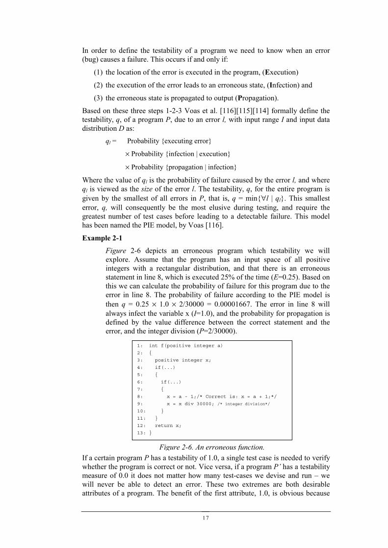
Figure 2-6 depicts an erroneous program which testability we willexplore. Assume that the program has an input space of all positiveintegers with a rectangular distribution, and that there is an erroneousstatement in line 8, which is executed 25% of the time (E=0.25). Based onthis we can calculate the probability of failure for this program due to theerror in line 8. The probability of failure according to the PIE model isthen q = 0.25 × 1.0 × 2/30000 = 0.00001667. The error in line 8 willalways infect the variable x (I=1.0), and the probability for propagation isdefined by the value difference between the correct statement and theerror, and the integer division (P=2/30000).

If a certain program P has a testability of 1.0, a single test case is needed to verifywhether the program is correct or not. Vice versa, if a program P’ has a testabilitymeasure of 0.0 it does not matter how many test-cases we devise and run – wewill never be able to detect an error. These two extremes are both desirableattributes of a program. The benefit of the first attribute, 1.0, is obvious because

1: int f(positive integer a)

2: {

3: positive integer x;

4: if(...)

5: {

6: if(...)

7: {

8: x = a - 1;/* Correct is: x = a + 1;*/

9: x = x div 30000; /* integer division*/

10: }

11: }

12: return x;

13: }

Figure 2-6. An erroneous function.

18

we can easily explore program correctness. The use of the second attribute, 0.0,might not be as obvious, but if we can never detect an error, it will never cause afailure either. A testability score of 1.0 is utopia for a tester and a testability scoreof 0.0 is utopia for a designer of fault-tolerance. A tester wants by all means todetect a failure, and a designer of fault-tolerance wants by all means to stop theexecution, infection and propagation of an error before it leads to a failure. Thereis thus a fundamental trade-off between testability and fault-tolerance.

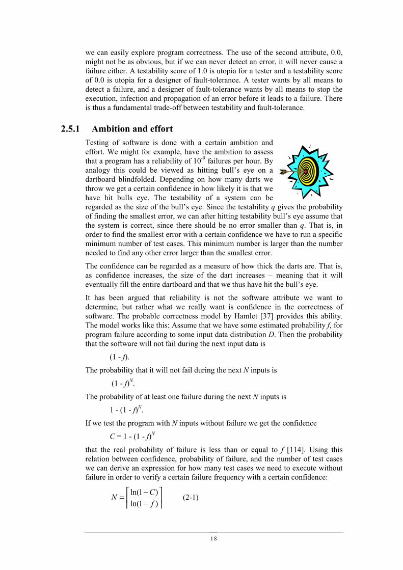
2.5.1 Ambition and effortTesting of software is done with a certain ambition andeffort. We might for example, have the ambition to assessthat a program has a reliability of 10-9 failures per hour. Byanalogy this could be viewed as hitting bull’s eye on adartboard blindfolded. Depending on how many darts wethrow we get a certain confidence in how likely it is that wehave hit bulls eye. The testability of a system can beregarded as the size of the bull’s eye. Since the testability q gives the probabilityof finding the smallest error, we can after hitting testability bull’s eye assume thatthe system is correct, since there should be no error smaller than q. That is, inorder to find the smallest error with a certain confidence we have to run a specificminimum number of test cases. This minimum number is larger than the numberneeded to find any other error larger than the smallest error.

The confidence can be regarded as a measure of how thick the darts are. That is,as confidence increases, the size of the dart increases – meaning that it willeventually fill the entire dartboard and that we thus have hit the bull’s eye.

It has been argued that reliability is not the software attribute we want todetermine, but rather what we really want is confidence in the correctness ofsoftware. The probable correctness model by Hamlet [37] provides this ability.The model works like this: Assume that we have some estimated probability f, forprogram failure according to some input data distribution D. Then the probabilitythat the software will not fail during the next input data is

(1 - f).

The probability that it will not fail during the next N inputs is

(1 - f)N.

The probability of at least one failure during the next N inputs is

1 - (1 - f)N.

If we test the program with N inputs without failure we get the confidence

C = 1 - (1 - f)N

that the real probability of failure is less than or equal to f [114]. Using thisrelation between confidence, probability of failure, and the number of test caseswe can derive an expression for how many test cases we need to execute withoutfailure in order to verify a certain failure frequency with a certain confidence:

−−=

)1ln()1ln(

fCN (2-1)

19

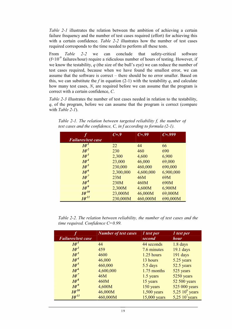
Table 2-1 illustrates the relation between the ambition of achieving a certainfailure frequency and the number of test cases required (effort) for achieving thiswith a certain confidence. Table 2-2 illustrates how the number of test casesrequired corresponds to the time needed to perform all these tests.

From Table 2-2 we can conclude that safety-critical software(f<10-9 failures/hour) require a ridiculous number of hours of testing. However, ifwe know the testability, q (the size of the bull’s eye) we can reduce the number oftest cases required, because when we have found the smallest error, we canassume that the software is correct – there should be no error smaller. Based onthis, we can substitute the f in equation (2-1) with the testability q, and calculatehow many test cases, N, are required before we can assume that the program iscorrect with a certain confidence, C.

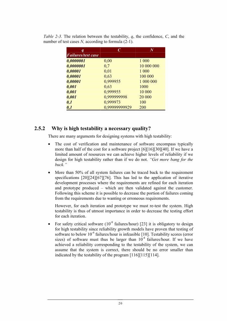
Table 2-3 illustrates the number of test cases needed in relation to the testability,q, of the program, before we can assume that the program is correct (comparewith Table 2-1).

Table 2-2. The relation between reliability, the number of test cases and thetime required. Confidence C=0.99.

fFailures/test case

Number of test cases 1 test persecond

1 test perhour

10-1 44 44 seconds 1.8 days10-2 459 7.6 minutes 19.1 days10-3 4600 1.25 hours 191 days10-4 46,000 13 hours 5.25 years10-5 460,000 5.5 days 52.5 years10-6 4,600,000 1.75 months 525 years10-7 46M 1.5 years 5250 years10-8 460M 15 years 52 500 years10-9 4,600M 150 years 525 000 years10-10 46,000M 1,500 years 5,25 106 years10-11 460,000M 15,000 years 5,25 107years

Table 2-1. The relation between targeted reliability f, the number oftest cases and the confidence, C, in f according to formula (2-1).

fFailures/test case

C=.9 C=.99 C=.999

10-1 22 44 6610-2 230 460 69010-3 2,300 4,600 6,90010-4 23,000 46,000 69,00010-5 230,000 460,000 690,00010-6 2,300,000 4,600,000 6,900,00010-7 23M 46M 69M10-8 230M 460M 690M10-9 2,300M 4,600M 6,900M10-10 23,000M 46,000M 69,000M10-11 230,000M 460,000M 690,000M

20

2.5.2 Why is high testability a necessary quality?There are many arguments for designing systems with high testability:

• The cost of verification and maintenance of software encompass typicallymore than half of the cost for a software project [6][16][30][40]. If we have alimited amount of resources we can achieve higher levels of reliability if wedesign for high testability rather than if we do not. “Get more bang for thebuck.”

• More than 50% of all system failures can be traced back to the requirementspecifications [20][24][67][76]. This has led to the application of iterativedevelopment processes where the requirements are refined for each iterationand prototype produced – which are then validated against the customer.Following this scheme it is possible to decrease the portion of failures comingfrom the requirements due to wanting or erroneous requirements.

However, for each iteration and prototype we must re-test the system. Hightestability is thus of utmost importance in order to decrease the testing effortfor each iteration.

• For safety critical software (10-9 failures/hour) [23] it is obligatory to designfor high testability since reliability growth models have proven that testing ofsoftware to below 10-4 failures/hour is infeasible [10]. Testability scores (errorsizes) of software must thus be larger than 10-4 failures/hour. If we haveachieved a reliability corresponding to the testability of the system, we canassume that the system is correct, there should be no error smaller thanindicated by the testability of the program [116][115][114].

qFailures/test case

C N

0,0000001 0,00 1 0000,0000001 0,7 10 000 0000,00001 0,01 1 0000,00001 0,63 100 0000,00001 0,999955 1 000 0000,001 0,63 10000,001 0,999955 10 0000,001 0,999999998 20 0000,1 0,999973 1000,1 0,99999999929 200

Table 2-3. The relation between the testability, q, the confidence, C, and thenumber of test cases N, according to formula (2-1).

21

2.6 SummaryIn this chapter we have given an introduction to the peculiarities of computersoftware. From that we conclude that the problems of designing and verifyingsoftware are fundamental in character: Software has discontinuous behavior, noinertia, and has no physical restrictions what so ever, except for time. Silver bullets,i.e., techniques or methods that solely will eliminate all bugs have shown to be myths[9][38][85]. Any Programming language, any formal method, any theory ofscheduling, any fault tolerance technique, and any testing technique will always beflawed or incomplete. To design reliable software we must thus make use of all theseconcepts in union. Consequently, we will never be able to eliminate testingcompletely. However, with respect to testing, debugging and monitoring of real-timesystems software there has been very little work done. We will therefore in theremainder of this thesis discuss and give solutions to the peculiarities of monitoring,debugging and testing of single program real-time systems, multitasking real-timesystems, and distributed real-time systems.

22

23

3 THE SYSTEM MODEL AND TERMINOLOGYIn this chapter we define a basic system model which we will refine and extend insubsequent chapters. We will also introduce basic terminology and vocabulary.

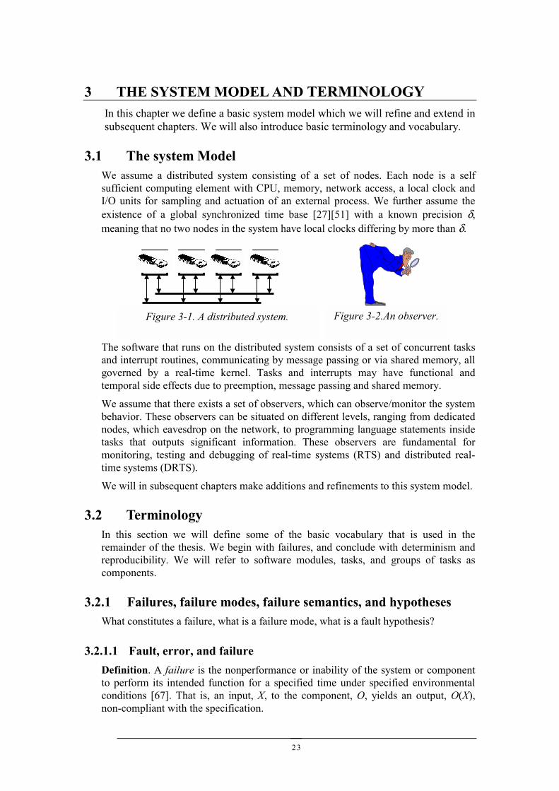
3.1 The system ModelWe assume a distributed system consisting of a set of nodes. Each node is a selfsufficient computing element with CPU, memory, network access, a local clock andI/O units for sampling and actuation of an external process. We further assume theexistence of a global synchronized time base [27][51] with a known precision δ,meaning that no two nodes in the system have local clocks differing by more than δ.

The software that runs on the distributed system consists of a set of concurrent tasksand interrupt routines, communicating by message passing or via shared memory, allgoverned by a real-time kernel. Tasks and interrupts may have functional andtemporal side effects due to preemption, message passing and shared memory.

We assume that there exists a set of observers, which can observe/monitor the systembehavior. These observers can be situated on different levels, ranging from dedicatednodes, which eavesdrop on the network, to programming language statements insidetasks that outputs significant information. These observers are fundamental formonitoring, testing and debugging of real-time systems (RTS) and distributed real-time systems (DRTS).

We will in subsequent chapters make additions and refinements to this system model.

3.2 TerminologyIn this section we will define some of the basic vocabulary that is used in theremainder of the thesis. We begin with failures, and conclude with determinism andreproducibility. We will refer to software modules, tasks, and groups of tasks ascomponents.

3.2.1 Failures, failure modes, failure semantics, and hypothesesWhat constitutes a failure, what is a failure mode, what is a fault hypothesis?

3.2.1.1 Fault, error, and failureDefinition. A failure is the nonperformance or inability of the system or componentto perform its intended function for a specified time under specified environmentalconditions [67]. That is, an input, X, to the component, O, yields an output, O(X),non-compliant with the specification.

Figure 3-1. A distributed system. Figure 3-2.An observer.

24

Definition. An error is a design flaw, or a deviation from a desired or intended state[67]. That is, if we view the program as a state machine, an error (bug) is anunwanted state. We can also view an error as a corrupted data state, caused by theexecution of an error (bug) but also due to e.g., physical electromagnetic radiation.

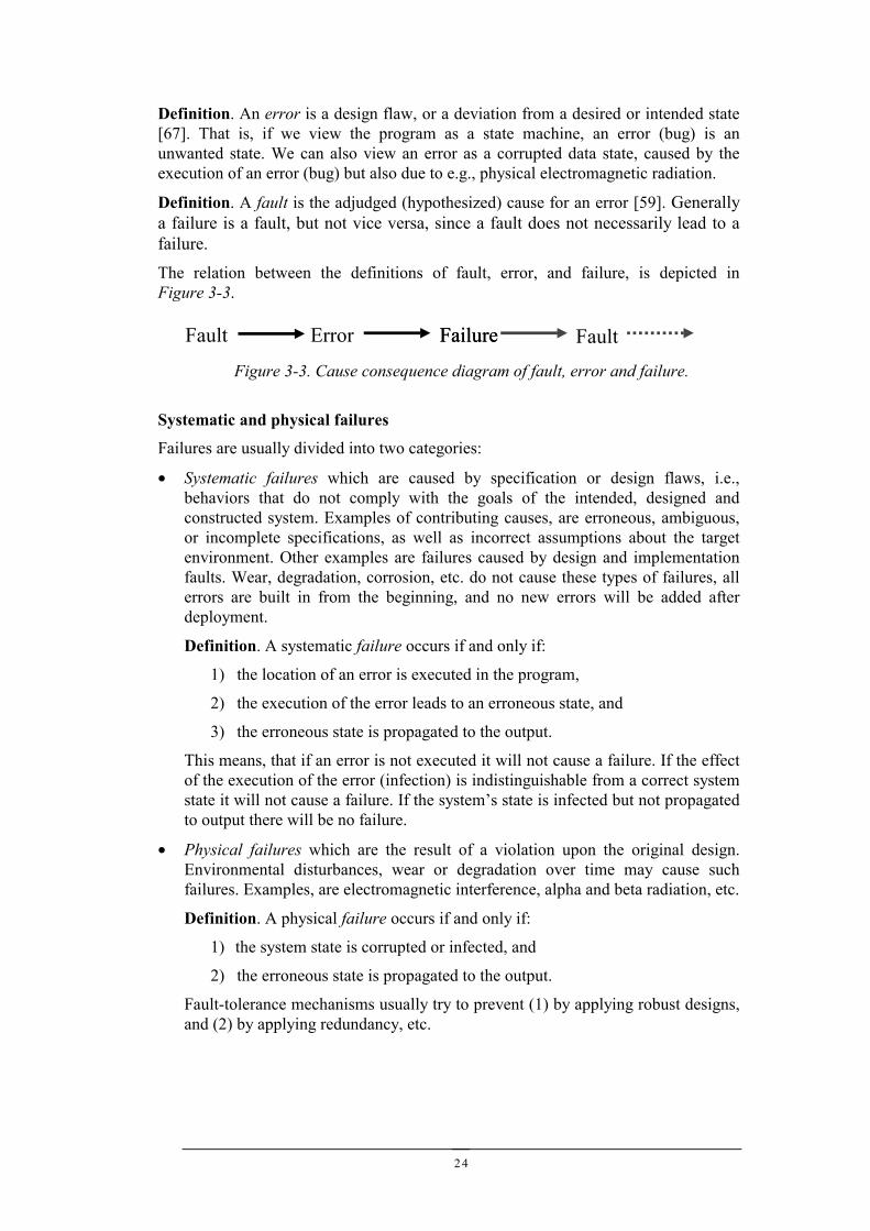
Definition. A fault is the adjudged (hypothesized) cause for an error [59]. Generallya failure is a fault, but not vice versa, since a fault does not necessarily lead to afailure.The relation between the definitions of fault, error, and failure, is depicted inFigure 3-3.

Systematic and physical failures

Failures are usually divided into two categories:

• Systematic failures which are caused by specification or design flaws, i.e.,behaviors that do not comply with the goals of the intended, designed andconstructed system. Examples of contributing causes, are erroneous, ambiguous,or incomplete specifications, as well as incorrect assumptions about the targetenvironment. Other examples are failures caused by design and implementationfaults. Wear, degradation, corrosion, etc. do not cause these types of failures, allerrors are built in from the beginning, and no new errors will be added afterdeployment.

Definition. A systematic failure occurs if and only if:

1) the location of an error is executed in the program,

2) the execution of the error leads to an erroneous state, and

3) the erroneous state is propagated to the output.

This means, that if an error is not executed it will not cause a failure. If the effectof the execution of the error (infection) is indistinguishable from a correct systemstate it will not cause a failure. If the system’s state is infected but not propagatedto output there will be no failure.

• Physical failures which are the result of a violation upon the original design.Environmental disturbances, wear or degradation over time may cause suchfailures. Examples, are electromagnetic interference, alpha and beta radiation, etc.

Definition. A physical failure occurs if and only if:

1) the system state is corrupted or infected, and

2) the erroneous state is propagated to the output.

Fault-tolerance mechanisms usually try to prevent (1) by applying robust designs,and (2) by applying redundancy, etc.

Fault Error FailureFailure FaultFigure 3-3. Cause consequence diagram of fault, error and failure.

25

3.2.1.2 Failure modesDepending on the architecture of the system we can assume different degrees, andclasses, of failure behavior. That is, certain types of failures are extremely improbable(impossible) in some systems, while in other systems it is very likely that they occur.For example, consider multitasking systems where we have to resolve access toshared resources by means of mutual exclusion. One approach is to make use ofsemaphores, and another to make use of separation in time. In the latter case deadlocksituations are impossible, while in the previous case deadlocks certainly are possible.Using synchronization in time we thus eliminate an entire class of failures, and cantherefore during testing eliminate the search for them.

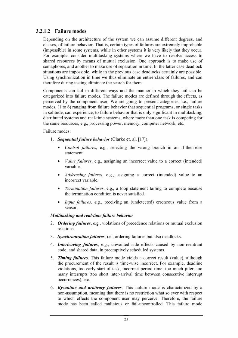
Components can fail in different ways and the manner in which they fail can becategorized into failure modes. The failure modes are defined through the effects, asperceived by the component user. We are going to present categories, i.e., failuremodes, (1 to 6) ranging from failure behavior that sequential programs, or single tasksin solitude, can experience, to failure behavior that is only significant in multitasking,distributed systems and real-time systems, where more than one task is competing forthe same resources, e.g., processing power, memory, computer network, etc.

Failure modes:

1. Sequential failure behavior (Clarke et. al. [17]):

• Control failures, e.g., selecting the wrong branch in an if-then-elsestatement.

• Value failures, e.g., assigning an incorrect value to a correct (intended)variable.

• Addressing failures, e.g., assigning a correct (intended) value to anincorrect variable.

• Termination failures, e.g., a loop statement failing to complete becausethe termination condition is never satisfied.

• Input failures, e.g., receiving an (undetected) erroneous value from asensor.

Multitasking and real-time failure behavior

2. Ordering failures, e.g., violations of precedence relations or mutual exclusionrelations.

3. Synchronization failures, i.e., ordering failures but also deadlocks.

4. Interleaving failures, e.g., unwanted side effects caused by non-reentrantcode, and shared data, in preemptively scheduled systems.

5. Timing failures. This failure mode yields a correct result (value), althoughthe procurement of the result is time-wise incorrect. For example, deadlineviolations, too early start of task, incorrect period time, too much jitter, toomany interrupts (too short inter-arrival time between consecutive interruptoccurrences), etc.

6. Byzantine and arbitrary failures. This failure mode is characterized by anon-assumption, meaning that there is no restriction what so ever with respectto which effects the component user may perceive. Therefore, the failuremode has been called malicious or fail-uncontrolled. This failure mode

26

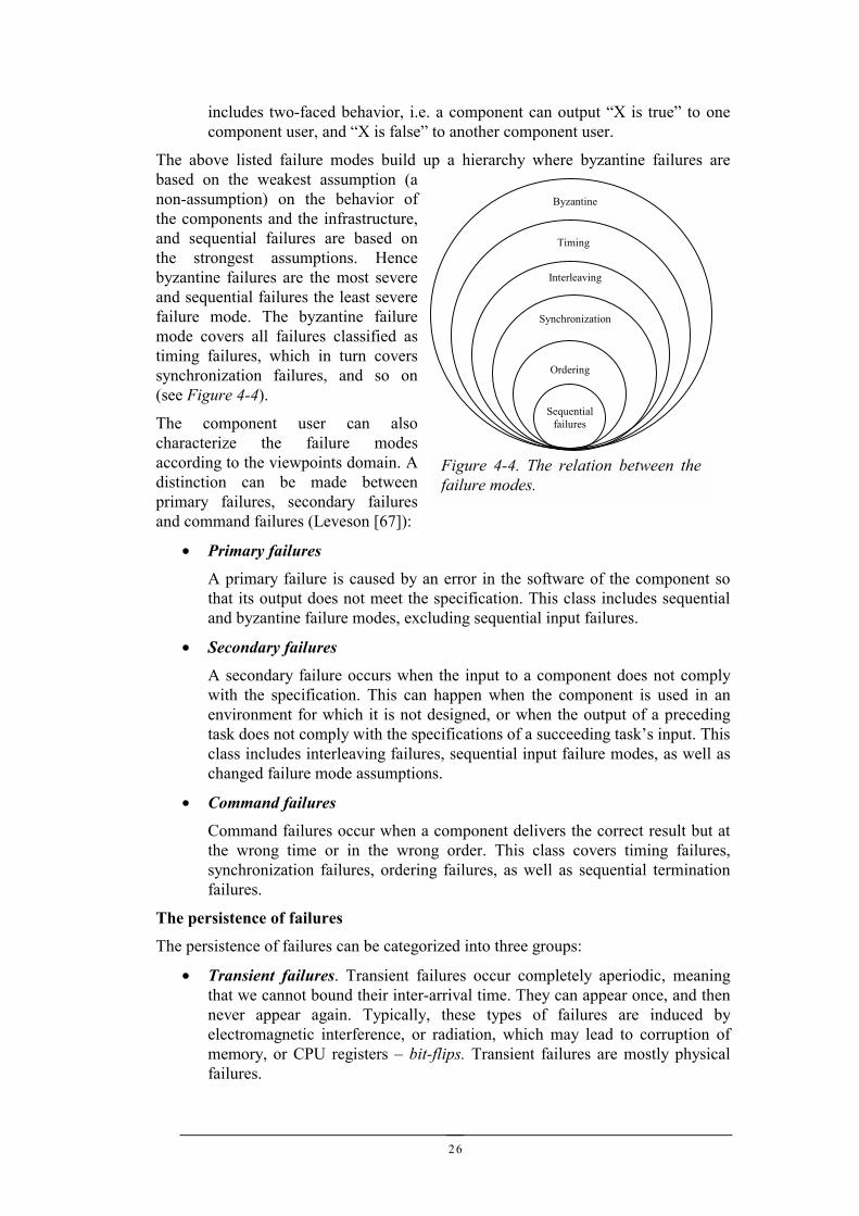
includes two-faced behavior, i.e. a component can output “X is true” to onecomponent user, and “X is false” to another component user.

The above listed failure modes build up a hierarchy where byzantine failures arebased on the weakest assumption (anon-assumption) on the behavior ofthe components and the infrastructure,and sequential failures are based onthe strongest assumptions. Hencebyzantine failures are the most severeand sequential failures the least severefailure mode. The byzantine failuremode covers all failures classified astiming failures, which in turn coverssynchronization failures, and so on(see Figure 4-4).

The component user can alsocharacterize the failure modesaccording to the viewpoints domain. Adistinction can be made betweenprimary failures, secondary failuresand command failures (Leveson [67]):

• Primary failures

A primary failure is caused by an error in the software of the component sothat its output does not meet the specification. This class includes sequentialand byzantine failure modes, excluding sequential input failures.

• Secondary failures

A secondary failure occurs when the input to a component does not complywith the specification. This can happen when the component is used in anenvironment for which it is not designed, or when the output of a precedingtask does not comply with the specifications of a succeeding task’s input. Thisclass includes interleaving failures, sequential input failure modes, as well aschanged failure mode assumptions.

• Command failures

Command failures occur when a component delivers the correct result but atthe wrong time or in the wrong order. This class covers timing failures,synchronization failures, ordering failures, as well as sequential terminationfailures.

The persistence of failures

The persistence of failures can be categorized into three groups:

• Transient failures. Transient failures occur completely aperiodic, meaningthat we cannot bound their inter-arrival time. They can appear once, and thennever appear again. Typically, these types of failures are induced byelectromagnetic interference, or radiation, which may lead to corruption ofmemory, or CPU registers – bit-flips. Transient failures are mostly physicalfailures.

Byzantine

Timing

Synchronization

Ordering

Sequentialfailures

Figure 4-4. The relation between thefailure modes.

Interleaving

27

• Intermittent failures. The inter-arrival time of intermittent failures can bebounded with a minimum and/or maximum inter-arrival time. These types offailures typically take place when a component is on the verge of breakingdown, for example, due to a glitch in a switch. Examples from the softwareworld could be failures due to sporadic interrupts.

• Permanent failures. A permanent failure that occurs, stays until removed(repaired). A permanent failure can be a damaged sensor, or typically forsoftware, a systematic failure – caused by an error in a program, which staysthere until removed.

3.2.1.3 Failure semanticsThe above classification of failure modes is not restricted to individual instances offailures, but can be used to classify the failure behavior of components, which iscalled a component’s failure semantics (Poledna [87]):

• Failure semantics

A component exhibits a given failure semantic if the probability of failure modes,which are not covered by the failure semantic, is sufficiently low.

If a given component is assumed to have synchronization failure semantics, then allindividual failures of the component should be synchronization-, ordering-, orsequential failures. The possibility of more severe failures, like timing failures, shouldbe sufficiently low. The failure semantic is a probabilistic specification of the failuremodes a component may exhibit. The semantic has to be chosen in relation to theapplication requirements. In other words, the failure semantics defines the mostsevere failure mode a component should experience. Fault-tolerant systems aredesigned with the assumption that any component that fails will do so according to agiven failure semantic. When we test a system we do so also with a certain failuresemantic in mind. That is, we look for failures of a certain kind. For plain sequentialprograms we usually do not look for interleaving failures, or timing failures.However, if the component will be used in a multitasking or real-time system wecertainly have to look for these types of failures.

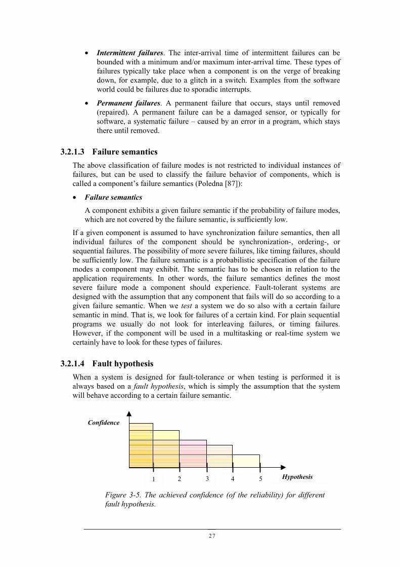
3.2.1.4 Fault hypothesisWhen a system is designed for fault-tolerance or when testing is performed it isalways based on a fault hypothesis, which is simply the assumption that the systemwill behave according to a certain failure semantic.

Confidence

2 4 Hypothesis51 3

Figure 3-5. The achieved confidence (of the reliability) for differentfault hypothesis.

28

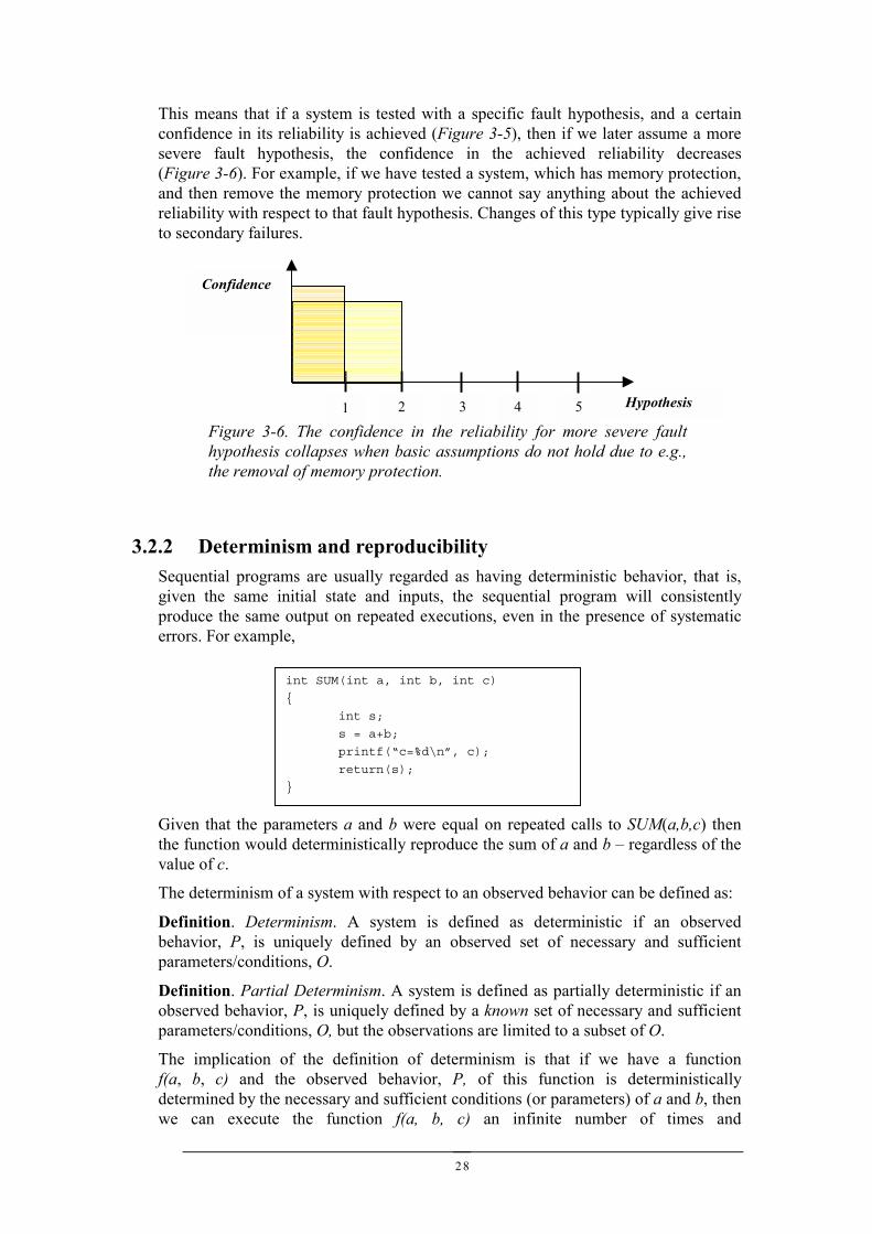
This means that if a system is tested with a specific fault hypothesis, and a certainconfidence in its reliability is achieved (Figure 3-5), then if we later assume a moresevere fault hypothesis, the confidence in the achieved reliability decreases(Figure 3-6). For example, if we have tested a system, which has memory protection,and then remove the memory protection we cannot say anything about the achievedreliability with respect to that fault hypothesis. Changes of this type typically give riseto secondary failures.

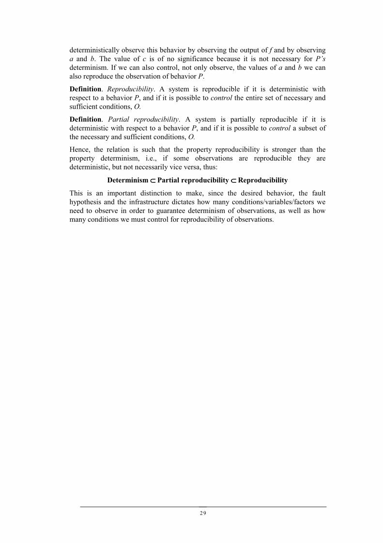
3.2.2 Determinism and reproducibilitySequential programs are usually regarded as having deterministic behavior, that is,given the same initial state and inputs, the sequential program will consistentlyproduce the same output on repeated executions, even in the presence of systematicerrors. For example,

Given that the parameters a and b were equal on repeated calls to SUM(a,b,c) thenthe function would deterministically reproduce the sum of a and b – regardless of thevalue of c.

The determinism of a system with respect to an observed behavior can be defined as:

Definition. Determinism. A system is defined as deterministic if an observedbehavior, P, is uniquely defined by an observed set of necessary and sufficientparameters/conditions, O.

Definition. Partial Determinism. A system is defined as partially deterministic if anobserved behavior, P, is uniquely defined by a known set of necessary and sufficientparameters/conditions, O, but the observations are limited to a subset of O.

The implication of the definition of determinism is that if we have a functionf(a, b, c) and the observed behavior, P, of this function is deterministicallydetermined by the necessary and sufficient conditions (or parameters) of a and b, thenwe can execute the function f(a, b, c) an infinite number of times and

int SUM(int a, int b, int c)

{

int s;

s = a+b;

printf(“c=%d\n”, c);

return(s);

}

Confidence

2 4 Hypothesis51 3

Figure 3-6. The confidence in the reliability for more severe faulthypothesis collapses when basic assumptions do not hold due to e.g.,the removal of memory protection.

29

deterministically observe this behavior by observing the output of f and by observinga and b. The value of c is of no significance because it is not necessary for P’sdeterminism. If we can also control, not only observe, the values of a and b we canalso reproduce the observation of behavior P.

Definition. Reproducibility. A system is reproducible if it is deterministic withrespect to a behavior P, and if it is possible to control the entire set of necessary andsufficient conditions, O.

Definition. Partial reproducibility. A system is partially reproducible if it isdeterministic with respect to a behavior P, and if it is possible to control a subset ofthe necessary and sufficient conditions, O.

Hence, the relation is such that the property reproducibility is stronger than theproperty determinism, i.e., if some observations are reproducible they aredeterministic, but not necessarily vice versa, thus:

Determinism ⊂⊂⊂⊂ Partial reproducibility ⊂⊂⊂⊂ Reproducibility

This is an important distinction to make, since the desired behavior, the faulthypothesis and the infrastructure dictates how many conditions/variables/factors weneed to observe in order to guarantee determinism of observations, as well as howmany conditions we must control for reproducibility of observations.

30

31

4 MONITORING DISTRIBUTED REAL-TIME SYSTEMSWe will in this chapter discuss how to observe the behavior of embedded real-timesystems (RTS), and how to observe and correlate observations between nodes indistributed real-time systems (DRTS). There are two significant differences betweendebugging and testing of software for desktop computers and embedded real-timesystems:

• It is more difficult to observe embedded computer systems, simply becausethey are embedded, and that they thus have very few interfaces to the outsideworld, and

• the actual act of observing RTS and DRTS can change their behavior.

In order to dynamically verify a system, i.e., to test or debug it, we must observe itsrun-time behavior and deem how well these observations comply with the systemrequirements. Fundamental in all physical sciences, as well as in testing of software,is the non-ambiguity, or determinism, of observations, and the ability to reproduceobservations. Of equal importance is that the actual act of observation does notdisturb, or intrude on, system behavior. If nonetheless the observations are intrusivethen it is imperative that their effect can be calculated and compensated for. If wecannot, there are no guarantees that the observations are accurate or reproducible.

Race conditions with respect to order of access to shared resources occur naturally inmulti-tasking real-time systems. Different inputs to the racing tasks may lead todifferent execution paths. These paths will in turn lead to different execution timesfor the tasks, which depending on the design may lead to different orders of access tothe shared resources. As a consequence there may be different system behaviors if theoutcome of the operations on the shared resources depend on the ordering ofaccesses.

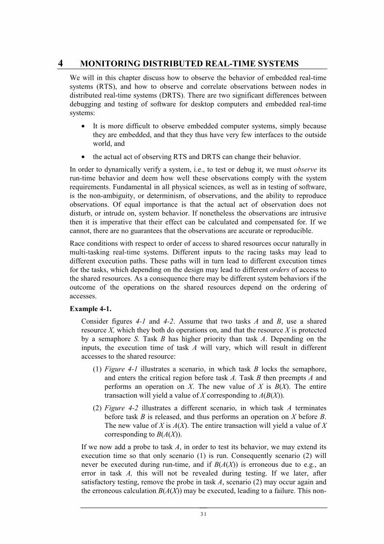
Example 4-1.

Consider figures 4-1 and 4-2. Assume that two tasks A and B, use a sharedresource X, which they both do operations on, and that the resource X is protectedby a semaphore S. Task B has higher priority than task A. Depending on theinputs, the execution time of task A will vary, which will result in differentaccesses to the shared resource:

(1) Figure 4-1 illustrates a scenario, in which task B locks the semaphore,and enters the critical region before task A. Task B then preempts A andperforms an operation on X. The new value of X is B(X). The entiretransaction will yield a value of X corresponding to A(B(X)).

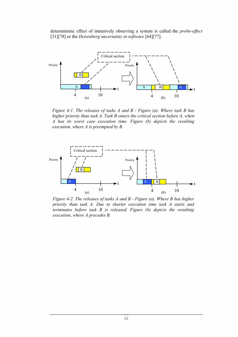
(2) Figure 4-2 illustrates a different scenario, in which task A terminatesbefore task B is released, and thus performs an operation on X before B.The new value of X is A(X). The entire transaction will yield a value of Xcorresponding to B(A(X)).

If we now add a probe to task A, in order to test its behavior, we may extend itsexecution time so that only scenario (1) is run. Consequently scenario (2) willnever be executed during run-time, and if B(A(X)) is erroneous due to e.g., anerror in task A, this will not be revealed during testing. If we later, aftersatisfactory testing, remove the probe in task A, scenario (2) may occur again andthe erroneous calculation B(A(X)) may be executed, leading to a failure. This non-

32

deterministic effect of intrusively observing a system is called the probe-effect[31][78] or the Heisenberg uncertainty in software [64][77].

Figure 4-1. The releases of tasks A and B - Figure (a). Where task B hashigher priority than task A. Task B enters the critical section before A, whenA has its worst case execution time. Figure (b) depicts the resultingexecution, where A is preempted by B.

t

Priority

4 10

B

A t

Priority

4 10

BA

Critical section

(a) (b)

A

t

Priority

4 10

Figure 4-2. The releases of tasks A and B - Figure (a). Where B has higherpriority than task A. Due to shorter execution time task A starts andterminates before task B is released. Figure (b) depicts the resultingexecution, where A precedes B.

B

A t

Priority

4 10

Critical section

(a) (b)

AA B

33

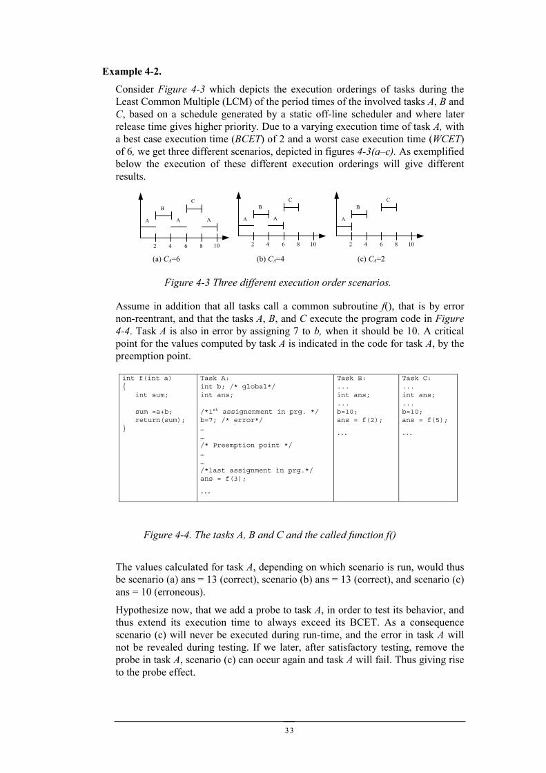
Example 4-2.

Consider Figure 4-3 which depicts the execution orderings of tasks during theLeast Common Multiple (LCM) of the period times of the involved tasks A, B andC, based on a schedule generated by a static off-line scheduler and where laterrelease time gives higher priority. Due to a varying execution time of task A, witha best case execution time (BCET) of 2 and a worst case execution time (WCET)of 6, we get three different scenarios, depicted in figures 4-3(a–c). As exemplifiedbelow the execution of these different execution orderings will give differentresults.

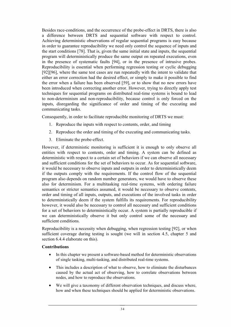
Assume in addition that all tasks call a common subroutine f(), that is by errornon-reentrant, and that the tasks A, B, and C execute the program code in Figure4-4. Task A is also in error by assigning 7 to b, when it should be 10. A criticalpoint for the values computed by task A is indicated in the code for task A, by thepreemption point.

The values calculated for task A, depending on which scenario is run, would thusbe scenario (a) ans = 13 (correct), scenario (b) ans = 13 (correct), and scenario (c)ans = 10 (erroneous).

Hypothesize now, that we add a probe to task A, in order to test its behavior, andthus extend its execution time to always exceed its BCET. As a consequencescenario (c) will never be executed during run-time, and the error in task A willnot be revealed during testing. If we later, after satisfactory testing, remove theprobe in task A, scenario (c) can occur again and task A will fail. Thus giving riseto the probe effect.

Figure 4-3 Three different execution order scenarios.

A A A

BC

2 4 6 8

A A

BC

2 4 6 8 1010

A

BC

2 4 6 8 10

(a) CA=6 (b) CA=4 (c) CA=2

Figure 4-4. The tasks A, B and C and the called function f()

int f(int a){

int sum;

sum =a+b;return(sum);

}

Task A:int b; /* global*/int ans;

/*1st assignenment in prg. */b=7; /* error*/……/* Preemption point */……/*last assignment in prg.*/ans = f(3);

…

Task B:...int ans;...b=10;ans = f(2);

…

Task C:...int ans;...b=10;ans = f(5);

…

34

Besides race-conditions, and the occurrence of the probe-effect in DRTS, there is alsoa difference between DRTS and sequential software with respect to control.Achieving deterministic observations of regular sequential programs is easy becausein order to guarantee reproducibility we need only control the sequence of inputs andthe start conditions [78]. That is, given the same initial state and inputs, the sequentialprogram will deterministically produce the same output on repeated executions, evenin the presence of systematic faults [94], or in the presence of intrusive probes.Reproducibility is essential when performing regression testing or cyclic debugging[92][96], where the same test cases are run repeatedly with the intent to validate thateither an error correction had the desired effect, or simply to make it possible to findthe error when a failure has been observed [59], or to show that no new errors havebeen introduced when correcting another error. However, trying to directly apply testtechniques for sequential programs on distributed real-time systems is bound to leadto non-determinism and non-reproducibility, because control is only forced on theinputs, disregarding the significance of order and timing of the executing andcommunicating tasks.

Consequently, in order to facilitate reproducible monitoring of DRTS we must:

1. Reproduce the inputs with respect to contents, order, and timing

2. Reproduce the order and timing of the executing and communicating tasks.

3. Eliminate the probe-effect.

However, if deterministic monitoring is sufficient it is enough to only observe allentities with respect to contents, order and timing. A system can be defined asdeterministic with respect to a certain set of behaviors if we can observe all necessaryand sufficient conditions for the set of behaviors to occur. As for sequential software,it would be necessary to observe inputs and outputs in order to deterministically deemif the outputs comply with the requirements. If the control flow of the sequentialprogram also depends on random number generators, we would have to observe thesealso for determinism. For a multitasking real-time systems, with ordering failuresemantics or stricter semantics assumed, it would be necessary to observe contents,order and timing of all inputs, outputs, and executions of the involved tasks in orderto deterministically deem if the system fulfills its requirements. For reproducibilityhowever, it would also be necessary to control all necessary and sufficient conditionsfor a set of behaviors to deterministically occur. A system is partially reproducible ifwe can deterministically observe it but only control some of the necessary andsufficient conditions.

Reproducibility is a necessity when debugging, when regression testing [92], or whensufficient coverage during testing is sought (we will in section 4.5, chapter 5 andsection 6.4.4 elaborate on this).

Contributions

• In this chapter we present a software-based method for deterministic observationsof single tasking, multi-tasking, and distributed real-time systems.

• This includes a description of what to observe, how to eliminate the disturbancescaused by the actual act of observing, how to correlate observations betweennodes, and how to reproduce the observations.

• We will give a taxonomy of different observation techniques, and discuss where,how and when these techniques should be applied for deterministic observations.

35

• We argue that it is essential to consider monitoring early in the design process, inorder to achieve efficient and deterministic observations.

4.1 MonitoringResearch on testing of shared memory multiprocessor systems and distributedsystems have been penetrated in some detail over the years. The focus has mainlybeen on monitoring, i.e. gathering of run-time information for debugging[86][111][112] and performance measurements [11].

The research issues have been:

• The intrusiveness (perturbation) of observations in software [31][64][78] andhow to eliminate the perturbations using special hardware [113].

• How to deterministically reproduce the observations using mechanisms insoftware [22][63] [104] or mechanisms in hardware [113]

• The problem of defining a global state in distributed systems [29] usinglogical clocks [12][58] or synchronized physical clocks [51][53][87].

However, the number of references on research regarding monitoring for testing anddebugging of single node real-time systems, and multiple node (distributed) real-timesystems, that consistently handle time, distribution, interrupts, clock synchronization,and scheduling, dwindle fast (to zip).

The observational requirements for testing and debugging differ, in the amount andtype of information required. The quintessential difference comes from the fact thattesting is used for finding failures (or showing their absence), while debugging is usedfor finding the errors that cause the failures. Another difference is that testing caneasily be automated, while debugging is essentially a manual task. For the verificationof safety-critical software (failure rates of 10-4 to 10-9 failures/hour) it is necessarythat the test process can be automated since the number of test cases required isenormous [10][70] (see chapter 2).

For testing of sequential programs it is usually sufficient to monitor inputs, andoutputs via predefined interfaces of the programs, and based on that informationdeem, according to the specification, if a test run was successful or not. For(distributed) real-time systems we need also observe the timing and order of theexecuting and communicating tasks, since the outputs depend on these variables, andthus also the determinism of the observations.

To detect errors using debugging it is also necessary to monitor the internal behaviorof the programs with respect to intermediate computed values, internal variables, andthe control flow. For interactive debugging, in the classical sense of sequentialprograms, it is required that the control flow can be altered via manual or conditionalbreakpoints, or via traces, all in order to be able to increase the observability of theprogram. Consequently, for debugging of (distributed) real-time systems, we need tocontrol the timing and order of the executing and communicating tasks, otherwise wecannot achieve deterministic debugging. However, the problem of defining a globalstate in distributed real-time systems, and break-pointing tasks on different nodes atexactly the same time, is a serious obstacle when debugging. Either we need to sendstop or continue messages from one node to a set of other nodes with the problem ofnonzero communication latencies, or we have a priori agreed upon times when theexecution on the processors should be halted or resumed. In the latter case there is theproblem of non-perfectly synchronized clocks, so the tasks may not halt or resume

36

their execution at the same time. Most real-time systems are also driven by theenvironment, so just because we breakpoint one task on one node, does not stop theexternal process.

When monitoring a DRTS there are some fundamental questions that must beanswered:

• How to extract enough information from the system?

• How to eliminate the perturbations that the observations cause?

• How to correlate the observations, i.e., how to define a consistent globalstate?

• How to reproduce the observations?

We are now going to address each of these questions in turn.

4.2 How to collect sufficient informationThe amount of monitoring needed in order to collect sufficient information isdependent on two basic factors:

• What is the fault hypothesis? That is, the more severe failure semantics, themore information we need to store and process in order to achievedeterministic observations. For sequential software it is sufficient to observeinputs and outputs. For multi-tasking systems we need also observe taskexecution orderings and their access to shared resources. For real-timesystems we further need to observe the timing of the tasks. However, if wewant to test a multitasking real-time system and assume sequential failuresemantics we need only test tasks in solitude, since we can regard each task asa sequential program. The probability that the multitasking real-time systemwill only exhibit sequential failure behavior in practice is not very highthough. It is therefore very important to chose a realistic fault-hypothesis andobserve the system based on that fault hypothesis.

• What is the a priori knowledge of the system with respect to its behavior andattributes? The validity of the fault-hypothesis is based on the support that theenvironment and the infrastructure (real-time kernel, hardware, etc.) give thefault hypothesis.

Does the system have memory protection? How does the system synchronizeaccess to shared resources (time or semaphores)? Is the execution strategytime-triggered or event-triggered?

For example, if the system is time-triggered and scheduled using e.g., strictperiodic fixed priority scheduling or static scheduling, we know that thesystem will repeat its execution every LCM. For event-triggered systems wehave no such general limit and might have to observe and store copiousamounts of information.

37

The actual information to be observed can be categorized into three groups:

• Data flow (internal and external)

• Control flow (execution and timing)

• Resources (memory and execution resources)

Data flow

• Inputs – determine for which input the task will execute, this is important ifthe actual input is not provided by a test oracle, but rather by an externalprocess or an environment simulator.

• Outputs – what are the produced outputs via the predefined interfaces of thetask? This includes messages that are passed between the system nodes, in aDRTS.

• Auxiliary outputs – output intermediately computed values, or program state,which are not visible via the predefined interfaces. For sequential softwarethese are commonly implemented using e.g., assertions, or even using printfstatements in C. For distributed real-time systems the situation is morecomplex and we need to define the type of data we additionally need.Typically these are related to memory mapped I/O interfaces, for examplereceived messages over the network, readings of A/D converters, readings ofthe local clock, etc. Because any additional outputs will require morememory, communication bandwidth, and execution time, we need to takethese auxiliary outputs into account when designing and scheduling, in orderto avoid the probe-effect. These auxiliary outputs could also beparameterized, i.e., we can during run-time switch between different auxiliaryoutputs, given of course that this parameterization is designed in such a waythat the timing behavior is constant.

Control flow

• Inputs, outputs, auxiliary outputs, and inter-node messages. At what time andin what order were the inputs received? At what time and in what order werethe outputs produced?

• Task switches – which, when, and in what order are tasks starting,preempting, and finishing? We can make use of this information for derivingthe synchronization and execution orderings between tasks. We can also makeuse of the timing information in order to deem if tasks start too early, too late,finish too late or finish too early. We can further measure the periodicity ofthe tasks and thus deem if jitter requirements are met. Making use of thistiming information we can also measure the execution times of the tasks.

• Interrupts – which, when, how long, and in what order are interruptsinterfering with tasks. Using this information we can judge how the interruptsinterfere with the execution of the tasks. We can thus measure if basicassumptions of interrupt overhead are true.

• Real-time kernel overhead. What is the execution time of the real-timekernel? What are the latencies due to interrupt disable, that is, when thekernel needs to perform atomic operations it usually disables all interferenceby interrupts, for how long time can the kernel block all interrupts?

38

• Tick rate. The tick rate is the frequency at which the real-time kernel isinvoked, and at which new scheduling decisions are taken. However, the tickrate can vary due to global clock synchronization. That is, the inter arrivaltime between ticks might increase or decrease if the local clock is to slow orto too fast compared to the global time base.

Resources

• Memory use – stack use, etc. How much of the memory is used by the tasks,interrupt service routines, or the kernel?

• CPU utilization. How much of the CPU’s calculating power is used?

• Network utilization. How much of the networks bandwidth is used?

• The state of the real-time kernel: Which tasks are waiting for their turn toexecute (waiting queue, list, or table)? Which task is running? Which tasksare blocked?

It is very important to deem which information is necessary for monitoring of thesystem, because if you extract too much there will be a heavy performance and costpenalty. If you extract too little, the precision of the observations will be too coarse orsimply non-deterministic for judging how and why the system behaved as it did. Fordeterminism there is a least necessary level of observability required, i.e., we need toobserve the necessary and sufficient parameters as defined in section 3.2.2. Anyadditional (useful) information surpassing the level of necessity for determinism willincrease the precision of the observations. Think of inputs, and outputs for sequentialsoftware as the least necessary level for determinism, while debugging provides ahigher level of observability (precision) since we can inspect the internal control flowand the contents of the variables.

4.3 Elimination of perturbationsAfter a decision on what entities to observe we need to decide on how to eliminatethe probe-effect. There are basically three approaches (1) non-intrusive/passivehardware, (2) intrusive software instrumentation, and a hybrid (3) where the softwareinstrumentation is minimized.

4.3.1 Hardware monitoringA transparent non-intrusive approach towards monitoring, is the application ofspecial hardware, e.g. hardware that allows buss sniffing, or non-intrusive access tomemory via dual-port memories, etc., but also through the use of hardware CPUemulators, (Lauterbach et al. [61]). Hardware monitoring has been applied forperformance measurements [8], execution monitoring of multiprocessor systems [73],and real-time systems [74][86][113]. Since the monitoring hardware is interfaced tothe target system’s hardware via the CPU socket (emulator) or via the data andaddress busses, it can observe the target system without interfering with its execution,and thus not introduce any probe-effects. The drawbacks are that the monitoringmechanisms must be very target specific and therefore very expensive, but also thatthe observations will be on a very low level of detail, since only the externalinterfaces of the microprocessors and shared resources such as dual-port memories,can be monitored. The ever-increasing integration of functionality in current general-purpose micro-controllers makes it correspondingly harder to observe the internalbehavior of the micro controllers/CPUs, due to cache memory, on-chip memory, etc.

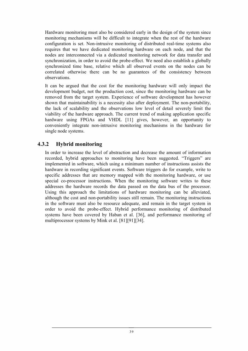
39

Hardware monitoring must also be considered early in the design of the system sincemonitoring mechanisms will be difficult to integrate when the rest of the hardwareconfiguration is set. Non-intrusive monitoring of distributed real-time systems alsorequires that we have dedicated monitoring hardware on each node, and that thenodes are interconnected via a dedicated monitoring network for data transfer andsynchronization, in order to avoid the probe-effect. We need also establish a globallysynchronized time base, relative which all observed events on the nodes can becorrelated otherwise there can be no guarantees of the consistency betweenobservations.

It can be argued that the cost for the monitoring hardware will only impact thedevelopment budget, not the production cost, since the monitoring hardware can beremoved from the target system. Experience of software development has howevershown that maintainability is a necessity also after deployment. The non-portability,the lack of scalability and the observations low level of detail severely limit theviability of the hardware approach. The current trend of making application specifichardware using FPGAs and VHDL [11] gives, however, an opportunity toconveniently integrate non-intrusive monitoring mechanisms in the hardware forsingle node systems.

4.3.2 Hybrid monitoringIn order to increase the level of abstraction and decrease the amount of informationrecorded, hybrid approaches to monitoring have been suggested. “Triggers” areimplemented in software, which using a minimum number of instructions assists thehardware in recording significant events. Software triggers do for example, write tospecific addresses that are memory mapped with the monitoring hardware, or usespecial co-processor instructions. When the monitoring software writes to theseaddresses the hardware records the data passed on the data bus of the processor.Using this approach the limitations of hardware monitoring can be alleviated,although the cost and non-portability issues still remain. The monitoring instructionsin the software must also be resource adequate, and remain in the target system inorder to avoid the probe-effect. Hybrid performance monitoring of distributedsystems have been covered by Haban et al. [36], and performance monitoring ofmultiprocessor systems by Mink et al. [81][91][34].

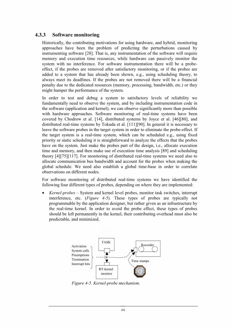
40

4.3.3 Software monitoringHistorically, the contributing motivations for using hardware, and hybrid, monitoringapproaches have been the problem of predicting the perturbations caused byinstrumenting software [28]. That is, any instrumentation of the software will requirememory and execution time resources, while hardware can passively monitor thesystem with no interference. For software instrumentation there will be a probe-effect, if the probes are removed after satisfactory monitoring, or if the probes areadded to a system that has already been shown, e.g., using scheduling theory, toalways meet its deadlines. If the probes are not removed there will be a financialpenalty due to the dedicated resources (memory, processing, bandwidth, etc.) or theymight hamper the performance of the system.

In order to test and debug a system to satisfactory levels of reliability wefundamentally need to observe the system, and by including instrumentation code inthe software (application and kernel), we can observe significantly more than possiblewith hardware approaches. Software monitoring of real-time systems have beencovered by Chodrow et al. [14], distributed systems by Joyce et al. [46][80], anddistributed real-time systems by Tokuda et al. [111][90]. In general it is necessary toleave the software probes in the target system in order to eliminate the probe-effect. Ifthe target system is a real-time system, which can be scheduled e.g., using fixedpriority or static scheduling it is straightforward to analyze the effects that the probeshave on the system. Just make the probes part of the design, i.e., allocate executiontime and memory, and then make use of execution time analysis [89] and schedulingtheory [4][75][117]. For monitoring of distributed real-time systems we need also toallocate communication bus bandwidth and account for the probes when making theglobal schedule. We need also establish a global time-base in order to correlateobservations on different nodes.

For software monitoring of distributed real-time systems we have identified thefollowing four different types of probes, depending on where they are implemented:

• Kernel-probes – System and kernel level probes, monitor task switches, interruptinterference, etc. (Figure 4-5). These types of probes are typically notprogrammable by the application designer, but rather given as an infrastructure bythe real-time kernel. In order to avoid the probe effect, these types of probesshould be left permanently in the kernel, their contributing overhead must also bepredictable, and minimized.

TASKRecorder

Time stamps

ActivationSystem callsPreemptionsTerminationInterrupt hits

RT-kernelmonitor

Figure 4-5. Kernel-probe mechanism.

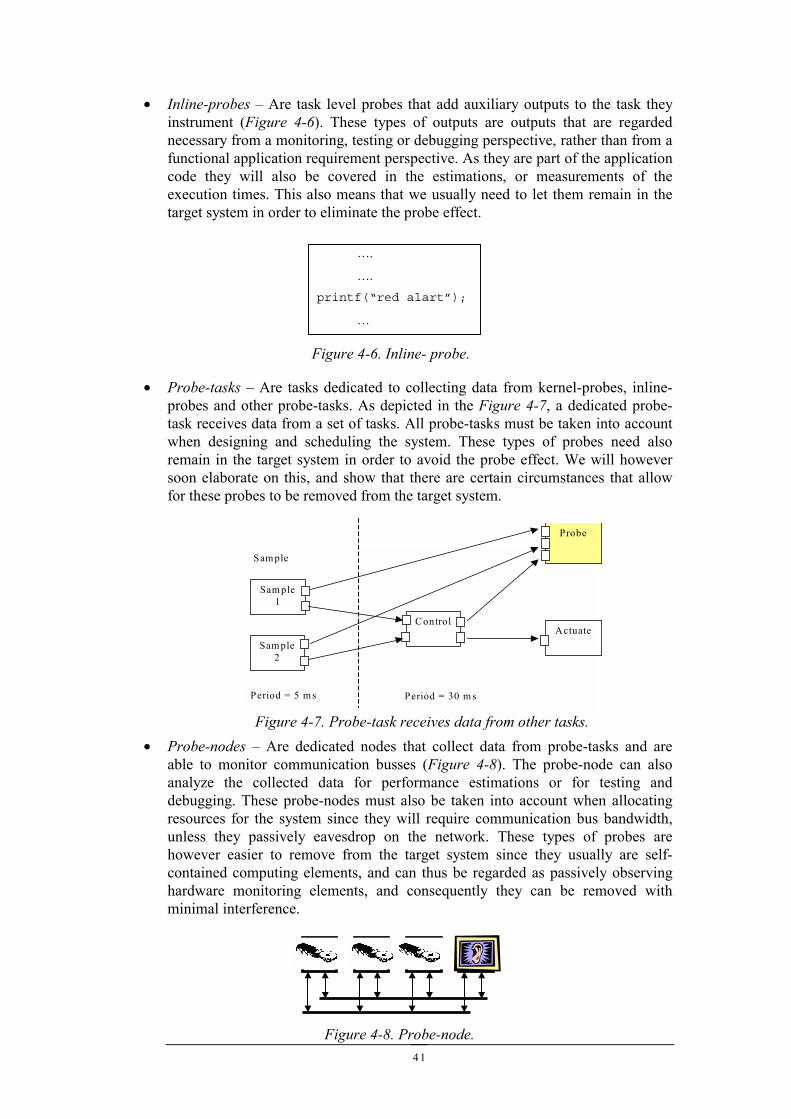
41

• Inline-probes – Are task level probes that add auxiliary outputs to the task theyinstrument (Figure 4-6). These types of outputs are outputs that are regardednecessary from a monitoring, testing or debugging perspective, rather than from afunctional application requirement perspective. As they are part of the applicationcode they will also be covered in the estimations, or measurements of theexecution times. This also means that we usually need to let them remain in thetarget system in order to eliminate the probe effect.

• Probe-tasks – Are tasks dedicated to collecting data from kernel-probes, inline-probes and other probe-tasks. As depicted in the Figure 4-7, a dedicated probe-task receives data from a set of tasks. All probe-tasks must be taken into accountwhen designing and scheduling the system. These types of probes need alsoremain in the target system in order to avoid the probe effect. We will howeversoon elaborate on this, and show that there are certain circumstances that allowfor these probes to be removed from the target system.

• Probe-nodes – Are dedicated nodes that collect data from probe-tasks and areable to monitor communication busses (Figure 4-8). The probe-node can alsoanalyze the collected data for performance estimations or for testing anddebugging. These probe-nodes must also be taken into account when allocatingresources for the system since they will require communication bus bandwidth,unless they passively eavesdrop on the network. These types of probes arehowever easier to remove from the target system since they usually are self-contained computing elements, and can thus be regarded as passively observinghardware monitoring elements, and consequently they can be removed withminimal interference.

….

….

printf(“red alart”);

…

Figure 4-6. Inline- probe.

Figure 4-8. Probe-node.

Sam ple

Sam ple1

ControlActuate

Sam ple2

Period = 5 m s Period = 30 m s

Probe

Figure 4-7. Probe-task receives data from other tasks.

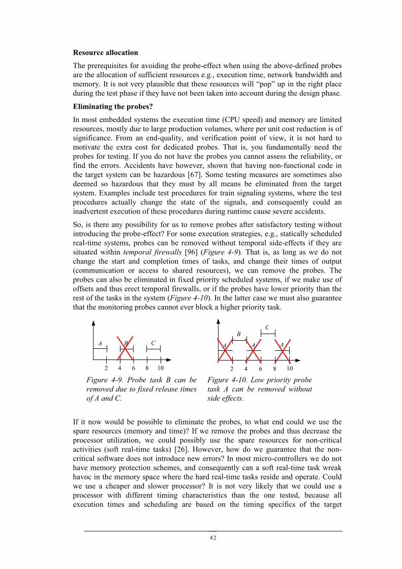
42

Resource allocation

The prerequisites for avoiding the probe-effect when using the above-defined probesare the allocation of sufficient resources e.g., execution time, network bandwidth andmemory. It is not very plausible that these resources will “pop” up in the right placeduring the test phase if they have not been taken into account during the design phase.

Eliminating the probes?

In most embedded systems the execution time (CPU speed) and memory are limitedresources, mostly due to large production volumes, where per unit cost reduction is ofsignificance. From an end-quality, and verification point of view, it is not hard tomotivate the extra cost for dedicated probes. That is, you fundamentally need theprobes for testing. If you do not have the probes you cannot assess the reliability, orfind the errors. Accidents have however, shown that having non-functional code inthe target system can be hazardous [67]. Some testing measures are sometimes alsodeemed so hazardous that they must by all means be eliminated from the targetsystem. Examples include test procedures for train signaling systems, where the testprocedures actually change the state of the signals, and consequently could aninadvertent execution of these procedures during runtime cause severe accidents.

So, is there any possibility for us to remove probes after satisfactory testing withoutintroducing the probe-effect? For some execution strategies, e.g., statically scheduledreal-time systems, probes can be removed without temporal side-effects if they aresituated within temporal firewalls [96] (Figure 4-9). That is, as long as we do notchange the start and completion times of tasks, and change their times of output(communication or access to shared resources), we can remove the probes. Theprobes can also be eliminated in fixed priority scheduled systems, if we make use ofoffsets and thus erect temporal firewalls, or if the probes have lower priority than therest of the tasks in the system (Figure 4-10). In the latter case we must also guaranteethat the monitoring probes cannot ever block a higher priority task.

If it now would be possible to eliminate the probes, to what end could we use thespare resources (memory and time)? If we remove the probes and thus decrease theprocessor utilization, we could possibly use the spare resources for non-criticalactivities (soft real-time tasks) [26]. However, how do we guarantee that the non-critical software does not introduce new errors? In most micro-controllers we do nothave memory protection schemes, and consequently can a soft real-time task wreakhavoc in the memory space where the hard real-time tasks reside and operate. Couldwe use a cheaper and slower processor? It is not very likely that we could use aprocessor with different timing characteristics than the one tested, because allexecution times and scheduling are based on the timing specifics of the target

A B C

2 4 6 8 10

Figure 4-9. Probe task B can beremoved due to fixed release timesof A and C.

A A AB

C

2 4 6 8 10

Figure 4-10. Low priority probetask A can be removed withoutside effects.

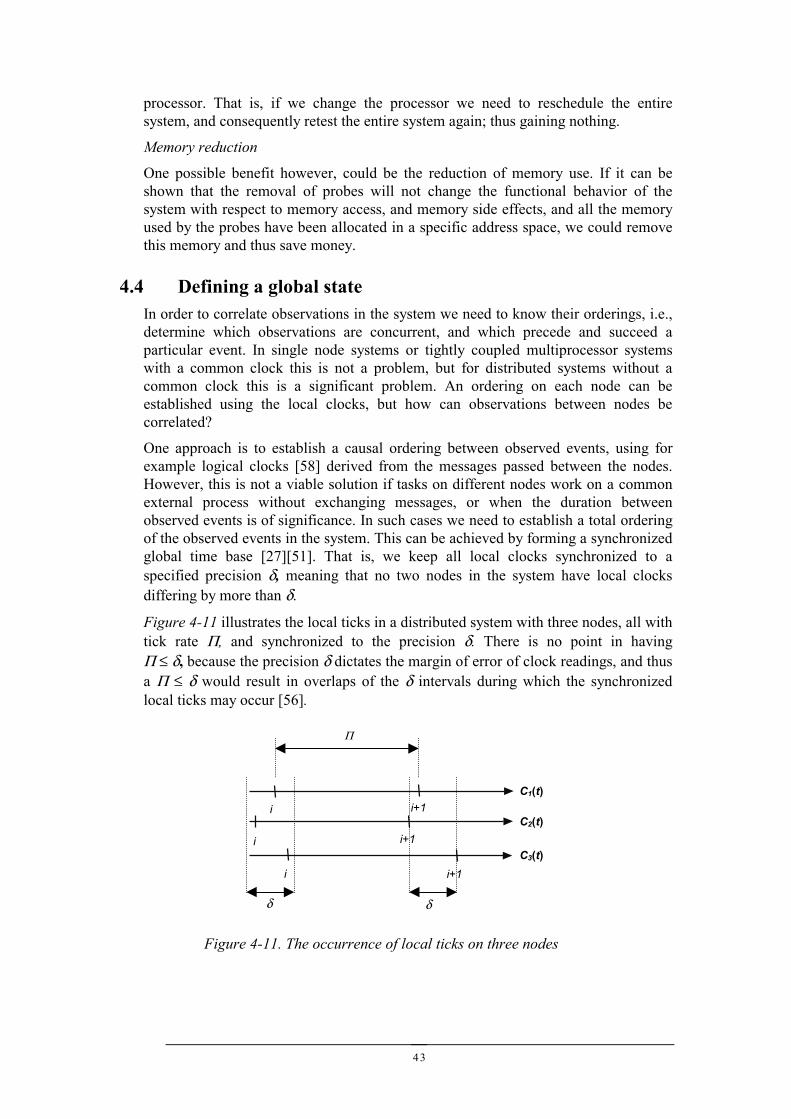
43

processor. That is, if we change the processor we need to reschedule the entiresystem, and consequently retest the entire system again; thus gaining nothing.

Memory reduction

One possible benefit however, could be the reduction of memory use. If it can beshown that the removal of probes will not change the functional behavior of thesystem with respect to memory access, and memory side effects, and all the memoryused by the probes have been allocated in a specific address space, we could removethis memory and thus save money.

4.4 Defining a global stateIn order to correlate observations in the system we need to know their orderings, i.e.,determine which observations are concurrent, and which precede and succeed aparticular event. In single node systems or tightly coupled multiprocessor systemswith a common clock this is not a problem, but for distributed systems without acommon clock this is a significant problem. An ordering on each node can beestablished using the local clocks, but how can observations between nodes becorrelated?

One approach is to establish a causal ordering between observed events, using forexample logical clocks [58] derived from the messages passed between the nodes.However, this is not a viable solution if tasks on different nodes work on a commonexternal process without exchanging messages, or when the duration betweenobserved events is of significance. In such cases we need to establish a total orderingof the observed events in the system. This can be achieved by forming a synchronizedglobal time base [27][51]. That is, we keep all local clocks synchronized to aspecified precision δ, meaning that no two nodes in the system have local clocksdiffering by more than δ.

Figure 4-11 illustrates the local ticks in a distributed system with three nodes, all withtick rate Π, and synchronized to the precision δ. There is no point in havingΠ ≤ δ, because the precision δ dictates the margin of error of clock readings, and thusa Π ≤ δ would result in overlaps of the δ intervals during which the synchronizedlocal ticks may occur [56].

Figure 4-11. The occurrence of local ticks on three nodes

δ δ

C1(t)i+1i

i+1

i+1

i

i

Π

C2(t)

C3(t)

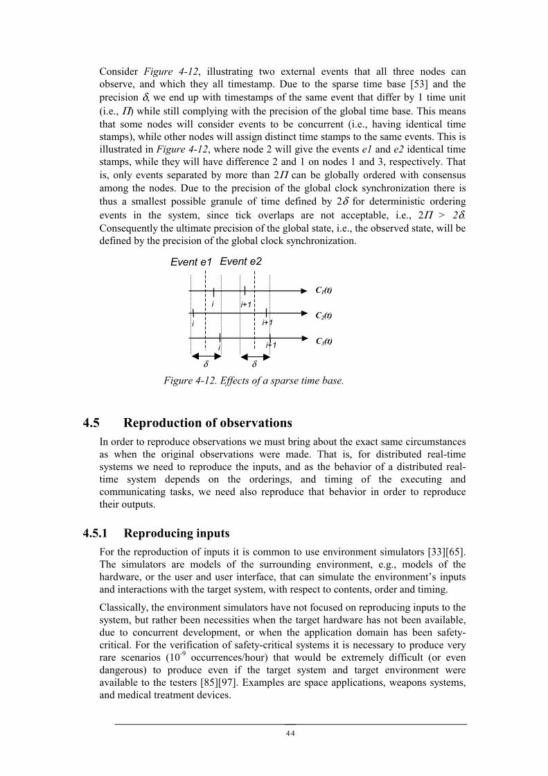
44

Consider Figure 4-12, illustrating two external events that all three nodes canobserve, and which they all timestamp. Due to the sparse time base [53] and theprecision δ, we end up with timestamps of the same event that differ by 1 time unit(i.e., Π) while still complying with the precision of the global time base. This meansthat some nodes will consider events to be concurrent (i.e., having identical timestamps), while other nodes will assign distinct time stamps to the same events. This isillustrated in Figure 4-12, where node 2 will give the events e1 and e2 identical timestamps, while they will have difference 2 and 1 on nodes 1 and 3, respectively. Thatis, only events separated by more than 2Π can be globally ordered with consensusamong the nodes. Due to the precision of the global clock synchronization there isthus a smallest possible granule of time defined by 2δ for deterministic orderingevents in the system, since tick overlaps are not acceptable, i.e., 2Π > 2δ.Consequently the ultimate precision of the global state, i.e., the observed state, will bedefined by the precision of the global clock synchronization.

4.5 Reproduction of observationsIn order to reproduce observations we must bring about the exact same circumstancesas when the original observations were made. That is, for distributed real-timesystems we need to reproduce the inputs, and as the behavior of a distributed real-time system depends on the orderings, and timing of the executing andcommunicating tasks, we need also reproduce that behavior in order to reproducetheir outputs.

4.5.1 Reproducing inputsFor the reproduction of inputs it is common to use environment simulators [33][65].The simulators are models of the surrounding environment, e.g., models of thehardware, or the user and user interface, that can simulate the environment’s inputsand interactions with the target system, with respect to contents, order and timing.

Classically, the environment simulators have not focused on reproducing inputs to thesystem, but rather been necessities when the target hardware has not been available,due to concurrent development, or when the application domain has been safety-critical. For the verification of safety-critical systems it is necessary to produce veryrare scenarios (10-9 occurrences/hour) that would be extremely difficult (or evendangerous) to produce even if the target system and target environment wereavailable to the testers [85][97]. Examples are space applications, weapons systems,and medical treatment devices.

Figure 4-12. Effects of a sparse time base.

Event e2Event e1

C1(t)

C2(t)

C3(t)

δ δ

i

i

i

i+1

i+1

i+1

45

4.5.2 Reproduction of complete system behaviorWhen it comes to the reproduction of the state and outputs of single tasking RTS,multitasking RTS and DRTS, with respect to the orderings, and timing of theexecuting and communicating tasks, there are two approaches:

(1) Off-line replays, i.e., record the runtime behavior and examine it whilereplaying it off-line.

(2) On-line reproduction, i.e., rerun the system while controlling all necessaryconditions.

We will in subsequent chapters discuss and give solutions to (1) and (2). That is,elaborate on how reproduction of observations can be made with respect todebugging and testing of distributed real-time systems.

4.6 SummaryWe have in this chapter presented a framework for monitoring single tasking, multi-tasking, and distributed real-time systems. This includes a description of what toobserve, how to eliminate the disturbances caused by the actual act of observing (theprobe effect), how to correlate observations (how to define a global state), and how toreproduce them. We have given a taxonomy of different observation techniques, andwhere, how and when these techniques should be applied to obtain deterministicobservations. We have argued that it is essential to consider monitoring early in thedesign process in order to achieve efficient and deterministic observations. Softwaremonitoring is also the preferable approach since it scales better than the hardwareapproaches. Software monitoring can compared to hardware monitoring also observethe system on many levels of abstraction while hardware monitoring is limited toobservation of low level details.

46

47

5 DEBUGGING DISTRIBUTED REAL-TIME SYSTEMSWe will in this chapter present a method for reproducible debugging of real-timesystems (RTS) and distributed real-time systems (DRTS). Classical debuggingtechniques used for cyclic debugging of sequential programs like breakpoints,watches and single stepping (tracing) cannot immediately be applied to real-timesystems software without sacrificing determinism and reproducibility. We will in thischapter discuss and describe a software based technique for achieving reproducibledebugging, based on on-line recording and off-line replay, that covers interleavingfailure semantics.

Testing is the process of revealing failures by exploring the runtime behavior of thesystem for violations of the specifications. Debugging on the other hand is concernedwith revealing the errors that cause the failures. The execution of an error infects thestate of the system, e.g., by infecting variables, memory, etc, and finally the infectedstate propagates to output. The process of debugging is thus to follow the trace of thefailure back to the error. In order to reveal the error it is imperative that we canreproduce the failure repeatedly. This requires knowledge of the start conditions anddeterministic executions. For sequential software with no real-time requirements it issufficient to apply the same input and the same internal state in order to reproduce afailure. For distributed real-time software the situation gets more complicated due totiming and ordering issues.

There are several problems to be solved in moving from debugging of sequentialprograms (as handled by standard commercial debuggers) to debugging of distributedreal-time programs. We will briefly discuss the main issues by making the transitionin three steps:

Debugging sequential real-time programs

In moving from debugging sequential non real-time programs to debuggingsequential real-time programs temporal constraints on interactions with the externalprocess have to be met. This means that classical debugging with breakpoints andsingle stepping (tracing) cannot be directly applied, since it would make timelyreproduction of outputs to the external process impossible. Likewise, using adebugger we cannot directly reproduce inputs to the system that depend on the timewhen the program is executed, e.g., readings of sensors and accesses to the local real-time clock. A mechanism, which during debugging faithfully and deterministicallyreproduces these interactions, is required.

Debugging multi-tasking real-time programs

In moving from debugging sequential real-time programs to debugging multitaskingreal-time programs executing on a single processor we must in addition havemechanisms for reproducing task interleavings. For example, we need to keep trackof preemptions, interrupts, and accesses to critical regions. That is, we must havemechanisms for reproducing the interactions and synchronizations between theexecuting tasks.

Reproducing rendezvous between tasks has been covered by Tai et al. [104], as havereproduction of interrupts and task-switches using special hardware, by Tsai et al.[113]. Reproducing interrupts and task switches using both special hardware andsoftware have been covered by Dodd et al. [22]. However, since both the two latterapproaches are relying on special hardware and profiling tools they are not very

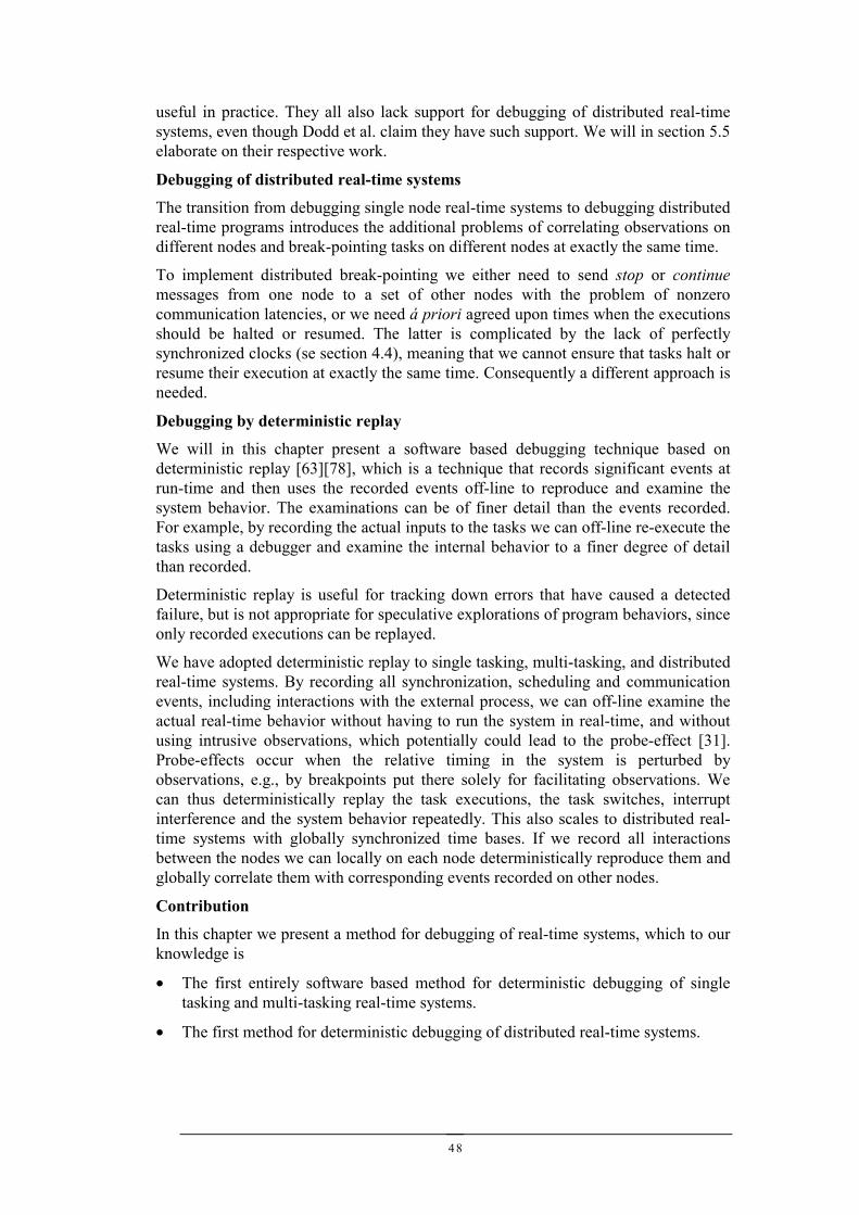
48

useful in practice. They all also lack support for debugging of distributed real-timesystems, even though Dodd et al. claim they have such support. We will in section 5.5elaborate on their respective work.

Debugging of distributed real-time systems

The transition from debugging single node real-time systems to debugging distributedreal-time programs introduces the additional problems of correlating observations ondifferent nodes and break-pointing tasks on different nodes at exactly the same time.

To implement distributed break-pointing we either need to send stop or continuemessages from one node to a set of other nodes with the problem of nonzerocommunication latencies, or we need á priori agreed upon times when the executionsshould be halted or resumed. The latter is complicated by the lack of perfectlysynchronized clocks (se section 4.4), meaning that we cannot ensure that tasks halt orresume their execution at exactly the same time. Consequently a different approach isneeded.

Debugging by deterministic replay

We will in this chapter present a software based debugging technique based ondeterministic replay [63][78], which is a technique that records significant events atrun-time and then uses the recorded events off-line to reproduce and examine thesystem behavior. The examinations can be of finer detail than the events recorded.For example, by recording the actual inputs to the tasks we can off-line re-execute thetasks using a debugger and examine the internal behavior to a finer degree of detailthan recorded.

Deterministic replay is useful for tracking down errors that have caused a detectedfailure, but is not appropriate for speculative explorations of program behaviors, sinceonly recorded executions can be replayed.

We have adopted deterministic replay to single tasking, multi-tasking, and distributedreal-time systems. By recording all synchronization, scheduling and communicationevents, including interactions with the external process, we can off-line examine theactual real-time behavior without having to run the system in real-time, and withoutusing intrusive observations, which potentially could lead to the probe-effect [31].Probe-effects occur when the relative timing in the system is perturbed byobservations, e.g., by breakpoints put there solely for facilitating observations. Wecan thus deterministically replay the task executions, the task switches, interruptinterference and the system behavior repeatedly. This also scales to distributed real-time systems with globally synchronized time bases. If we record all interactionsbetween the nodes we can locally on each node deterministically reproduce them andglobally correlate them with corresponding events recorded on other nodes.

Contribution

In this chapter we present a method for debugging of real-time systems, which to ourknowledge is

• The first entirely software based method for deterministic debugging of singletasking and multi-tasking real-time systems.

• The first method for deterministic debugging of distributed real-time systems.

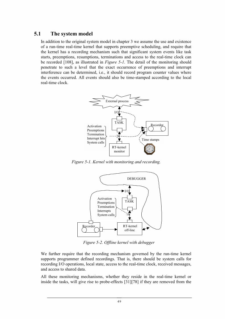
49

5.1 The system modelIn addition to the original system model in chapter 3 we assume the use and existenceof a run-time real-time kernel that supports preemptive scheduling, and require thatthe kernel has a recording mechanism such that significant system events like taskstarts, preemptions, resumptions, terminations and access to the real-time clock canbe recorded [108], as illustrated in Figure 5-1. The detail of the monitoring shouldpenetrate to such a level that the exact occurrence of preemptions and interruptinterference can be determined, i.e., it should record program counter values wherethe events occurred. All events should also be time-stamped according to the localreal-time clock.

We further require that the recording mechanism governed by the run-time kernelsupports programmer defined recordings. That is, there should be system calls forrecording I/O operations, local state, access to the real-time clock, received messages,and access to shared data.

All these monitoring mechanisms, whether they reside in the real-time kernel orinside the tasks, will give rise to probe-effects [31][78] if they are removed from the

TASKRecorder

Time stamps

External process

I/O

ActivationPreemptionsTerminationInterrupt hitsSystem calls

RT-kernelmonitor

Figure 5-1. Kernel with monitoring and recording.

Figure 5-2. Offline kernel with debugger

TASK

Recorder

I/O

ActivationPreemptionsTerminationInterruptsSystem calls

RT-kerneloff-line

DEBUGGER

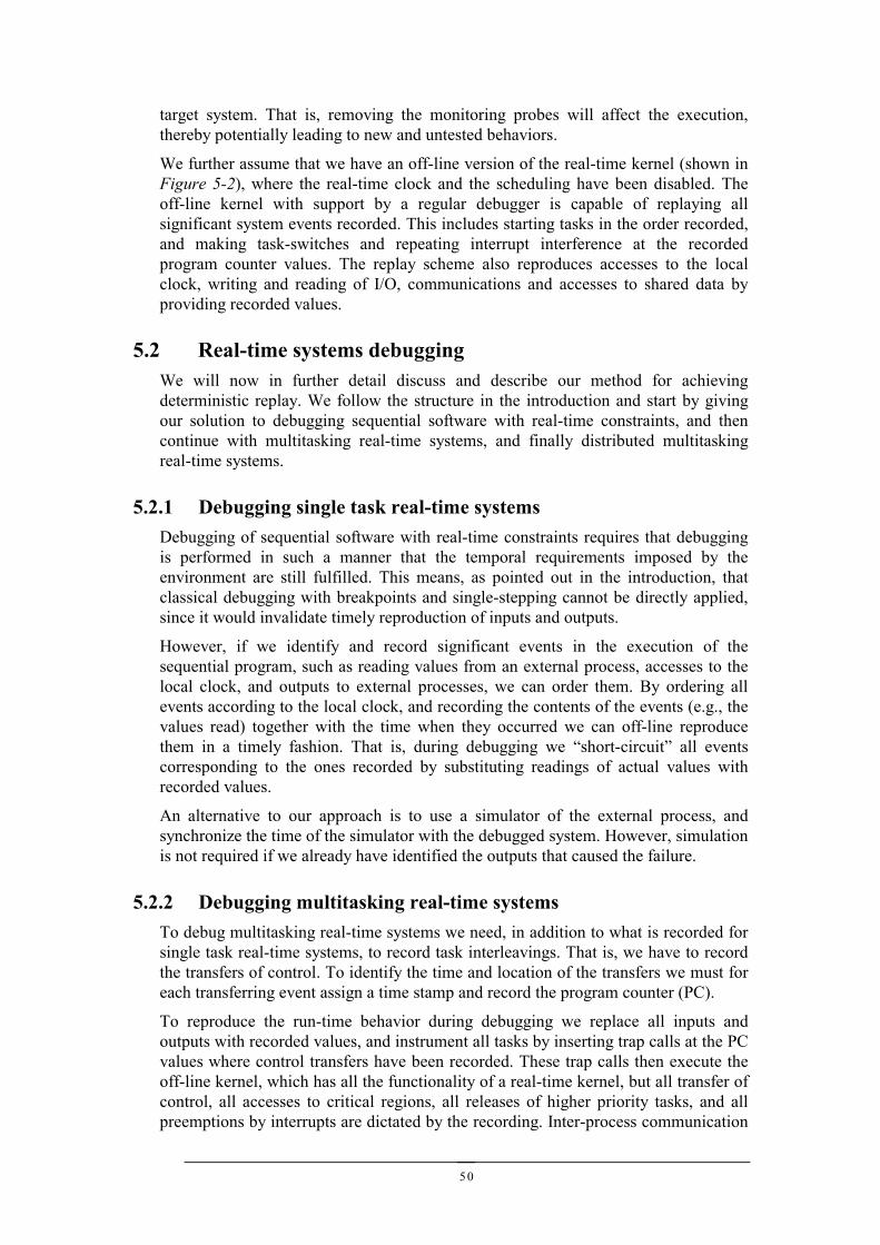
50

target system. That is, removing the monitoring probes will affect the execution,thereby potentially leading to new and untested behaviors.

We further assume that we have an off-line version of the real-time kernel (shown inFigure 5-2), where the real-time clock and the scheduling have been disabled. Theoff-line kernel with support by a regular debugger is capable of replaying allsignificant system events recorded. This includes starting tasks in the order recorded,and making task-switches and repeating interrupt interference at the recordedprogram counter values. The replay scheme also reproduces accesses to the localclock, writing and reading of I/O, communications and accesses to shared data byproviding recorded values.

5.2 Real-time systems debuggingWe will now in further detail discuss and describe our method for achievingdeterministic replay. We follow the structure in the introduction and start by givingour solution to debugging sequential software with real-time constraints, and thencontinue with multitasking real-time systems, and finally distributed multitaskingreal-time systems.

5.2.1 Debugging single task real-time systemsDebugging of sequential software with real-time constraints requires that debuggingis performed in such a manner that the temporal requirements imposed by theenvironment are still fulfilled. This means, as pointed out in the introduction, thatclassical debugging with breakpoints and single-stepping cannot be directly applied,since it would invalidate timely reproduction of inputs and outputs.

However, if we identify and record significant events in the execution of thesequential program, such as reading values from an external process, accesses to thelocal clock, and outputs to external processes, we can order them. By ordering allevents according to the local clock, and recording the contents of the events (e.g., thevalues read) together with the time when they occurred we can off-line reproducethem in a timely fashion. That is, during debugging we “short-circuit” all eventscorresponding to the ones recorded by substituting readings of actual values withrecorded values.

An alternative to our approach is to use a simulator of the external process, andsynchronize the time of the simulator with the debugged system. However, simulationis not required if we already have identified the outputs that caused the failure.

5.2.2 Debugging multitasking real-time systemsTo debug multitasking real-time systems we need, in addition to what is recorded forsingle task real-time systems, to record task interleavings. That is, we have to recordthe transfers of control. To identify the time and location of the transfers we must foreach transferring event assign a time stamp and record the program counter (PC).

To reproduce the run-time behavior during debugging we replace all inputs andoutputs with recorded values, and instrument all tasks by inserting trap calls at the PCvalues where control transfers have been recorded. These trap calls then execute theoff-line kernel, which has all the functionality of a real-time kernel, but all transfer ofcontrol, all accesses to critical regions, all releases of higher priority tasks, and allpreemptions by interrupts are dictated by the recording. Inter-process communication

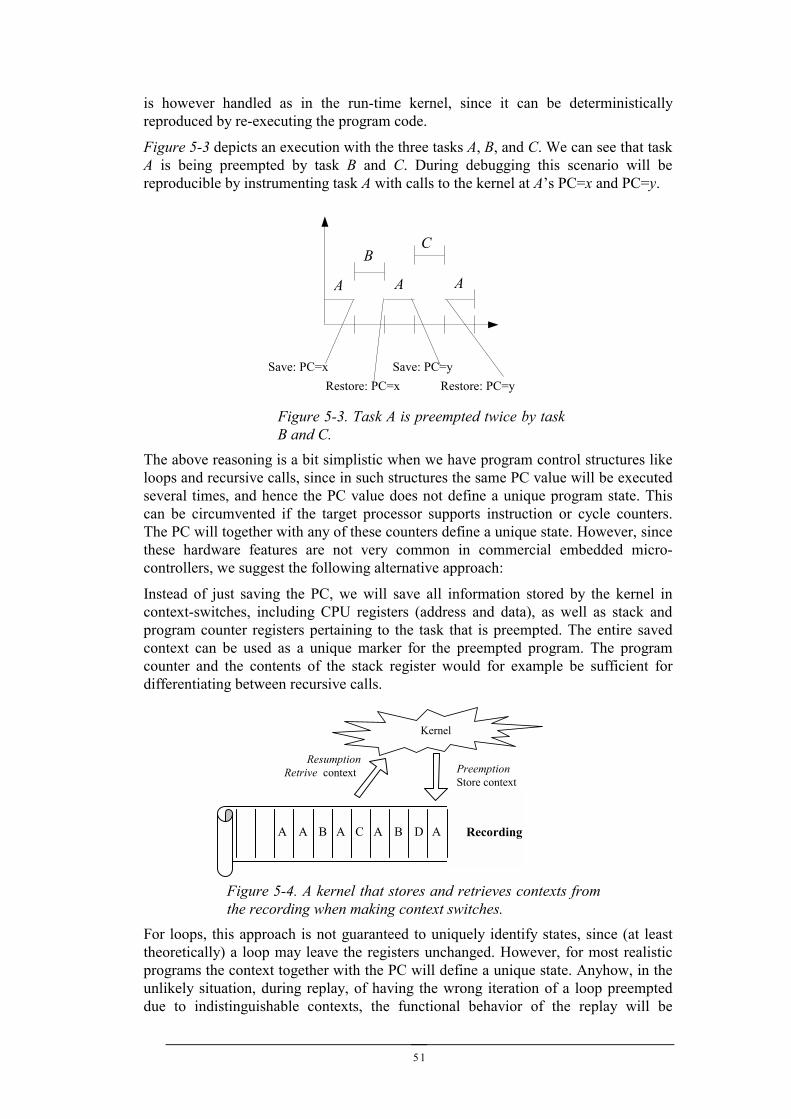
51

is however handled as in the run-time kernel, since it can be deterministicallyreproduced by re-executing the program code.

Figure 5-3 depicts an execution with the three tasks A, B, and C. We can see that taskA is being preempted by task B and C. During debugging this scenario will bereproducible by instrumenting task A with calls to the kernel at A’s PC=x and PC=y.

The above reasoning is a bit simplistic when we have program control structures likeloops and recursive calls, since in such structures the same PC value will be executedseveral times, and hence the PC value does not define a unique program state. Thiscan be circumvented if the target processor supports instruction or cycle counters.The PC will together with any of these counters define a unique state. However, sincethese hardware features are not very common in commercial embedded micro-controllers, we suggest the following alternative approach:

Instead of just saving the PC, we will save all information stored by the kernel incontext-switches, including CPU registers (address and data), as well as stack andprogram counter registers pertaining to the task that is preempted. The entire savedcontext can be used as a unique marker for the preempted program. The programcounter and the contents of the stack register would for example be sufficient fordifferentiating between recursive calls.

For loops, this approach is not guaranteed to uniquely identify states, since (at leasttheoretically) a loop may leave the registers unchanged. However, for most realisticprograms the context together with the PC will define a unique state. Anyhow, in theunlikely situation, during replay, of having the wrong iteration of a loop preempteddue to indistinguishable contexts, the functional behavior of the replay will be

A A A

BC

Figure 5-3. Task A is preempted twice by taskB and C.

Save: PC=xRestore: PC=x

Save: PC=yRestore: PC=y

Figure 5-4. A kernel that stores and retrieves contexts fromthe recording when making context switches.

ADBACABAA

Kernel

PreemptionStore context

ResumptionRetrive context

Recording

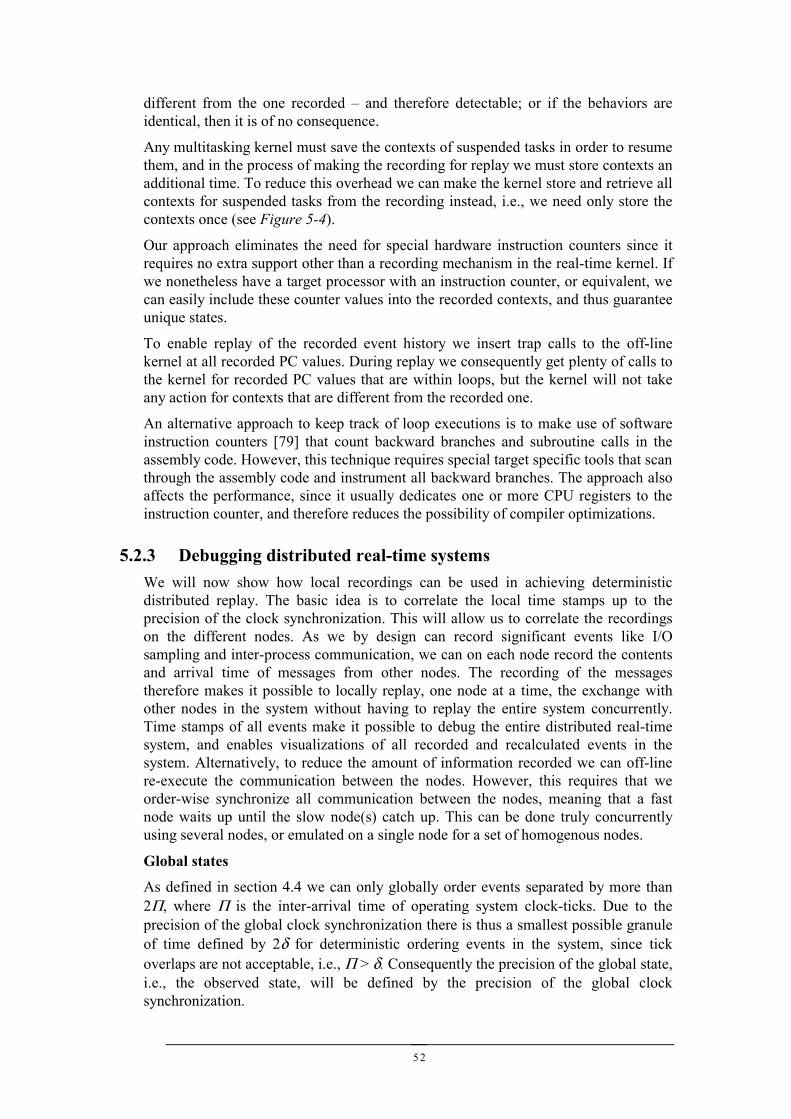
52

different from the one recorded – and therefore detectable; or if the behaviors areidentical, then it is of no consequence.

Any multitasking kernel must save the contexts of suspended tasks in order to resumethem, and in the process of making the recording for replay we must store contexts anadditional time. To reduce this overhead we can make the kernel store and retrieve allcontexts for suspended tasks from the recording instead, i.e., we need only store thecontexts once (see Figure 5-4).

Our approach eliminates the need for special hardware instruction counters since itrequires no extra support other than a recording mechanism in the real-time kernel. Ifwe nonetheless have a target processor with an instruction counter, or equivalent, wecan easily include these counter values into the recorded contexts, and thus guaranteeunique states.

To enable replay of the recorded event history we insert trap calls to the off-linekernel at all recorded PC values. During replay we consequently get plenty of calls tothe kernel for recorded PC values that are within loops, but the kernel will not takeany action for contexts that are different from the recorded one.

An alternative approach to keep track of loop executions is to make use of softwareinstruction counters [79] that count backward branches and subroutine calls in theassembly code. However, this technique requires special target specific tools that scanthrough the assembly code and instrument all backward branches. The approach alsoaffects the performance, since it usually dedicates one or more CPU registers to theinstruction counter, and therefore reduces the possibility of compiler optimizations.

5.2.3 Debugging distributed real-time systemsWe will now show how local recordings can be used in achieving deterministicdistributed replay. The basic idea is to correlate the local time stamps up to theprecision of the clock synchronization. This will allow us to correlate the recordingson the different nodes. As we by design can record significant events like I/Osampling and inter-process communication, we can on each node record the contentsand arrival time of messages from other nodes. The recording of the messagestherefore makes it possible to locally replay, one node at a time, the exchange withother nodes in the system without having to replay the entire system concurrently.Time stamps of all events make it possible to debug the entire distributed real-timesystem, and enables visualizations of all recorded and recalculated events in thesystem. Alternatively, to reduce the amount of information recorded we can off-linere-execute the communication between the nodes. However, this requires that weorder-wise synchronize all communication between the nodes, meaning that a fastnode waits up until the slow node(s) catch up. This can be done truly concurrentlyusing several nodes, or emulated on a single node for a set of homogenous nodes.

Global states

As defined in section 4.4 we can only globally order events separated by more than2Π, where Π is the inter-arrival time of operating system clock-ticks. Due to theprecision of the global clock synchronization there is thus a smallest possible granuleof time defined by 2δ for deterministic ordering events in the system, since tickoverlaps are not acceptable, i.e., Π > δ. Consequently the precision of the global state,i.e., the observed state, will be defined by the precision of the global clocksynchronization.

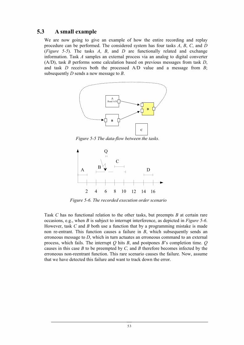
53

5.3 A small exampleWe are now going to give an example of how the entire recording and replayprocedure can be performed. The considered system has four tasks A, B, C, and D(Figure 5-5). The tasks A, B, and D are functionally related and exchangeinformation. Task A samples an external process via an analog to digital converter(A/D), task B performs some calculation based on previous messages from task D,and task D receives both the processed A/D value and a message from B;subsequently D sends a new message to B.

Task C has no functional relation to the other tasks, but preempts B at certain rareoccasions, e.g., when B is subject to interrupt interference, as depicted in Figure 5-6.However, task C and B both use a function that by a programming mistake is madenon re-entrant. This function causes a failure in B, which subsequently sends anerroneous message to D, which in turn actuates an erroneous command to an externalprocess, which fails. The interrupt Q hits B, and postpones B’s completion time. Qcauses in this case B to be preempted by C, and B therefore becomes infected by theerroneous non-reentrant function. This rare scenario causes the failure. Now, assumethat we have detected this failure and want to track down the error.

ARead A/D

C

B

D

Figure 5-5 The data-flow between the tasks.

2

BC

4 6 8 10

A D

12 14 16

Figure 5-6. The recorded execution order scenario

Q

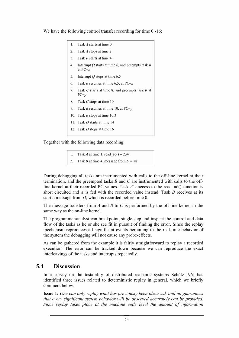
54

We have the following control transfer recording for time 0 -16:

Together with the following data recording:

During debugging all tasks are instrumented with calls to the off-line kernel at theirtermination, and the preempted tasks B and C are instrumented with calls to the off-line kernel at their recorded PC values. Task A’s access to the read_ad() function isshort circuited and A is fed with the recorded value instead. Task B receives at itsstart a message from D, which is recorded before time 0.

The message transfers from A and B to C is performed by the off-line kernel in thesame way as the on-line kernel.

The programmer/analyst can breakpoint, single step and inspect the control and dataflow of the tasks as he or she see fit in pursuit of finding the error. Since the replaymechanism reproduces all significant events pertaining to the real-time behavior ofthe system the debugging will not cause any probe-effects.

As can be gathered from the example it is fairly straightforward to replay a recordedexecution. The error can be tracked down because we can reproduce the exactinterleavings of the tasks and interrupts repeatedly.

5.4 DiscussionIn a survey on the testability of distributed real-time systems Schütz [96] hasidentified three issues related to deterministic replay in general, which we brieflycomment below:

Issue 1: One can only replay what has previously been observed, and no guaranteesthat every significant system behavior will be observed accurately can be provided.Since replay takes place at the machine code level the amount of information

1. Task A at time 1, read_ad() = 234

2. Task B at time 4, message from D = 78

1. Task A starts at time 0

2. Task A stops at time 2

3. Task B starts at time 4

4. Interrupt Q starts at time 6, and preempts task Bat PC=x

5. Interrupt Q stops at time 6,5

6. Task B resumes at time 6,5, at PC=x

7. Task C starts at time 8, and preempts task B atPC=y

8. Task C stops at time 10

9. Task B resumes at time 10, at PC=y

10. Task B stops at time 10,3

11. Task D starts at time 14

12. Task D stops at time 16

55

required is usually large. All inputs and intermediate events, e.g. messages, must bekept.

The amount and the necessary information required is of course a design issue, but itis not true that all inputs and intermediate messages must be recorded. The replay canas we have shown actually re-execute the tasks in the recorded event history. Onlythose inputs and messages which are not re-calculated, or re-sent, during the replaymust be kept. This is specifically the case for RTS with periodic tasks, where we canmake use of the knowledge of the schedule (precedence relations) and the durationbefore the schedule repeats it self (the LCM – the Least Common Multiple of the taskperiod times.) In systems where deterministic replay has previously been employed,e.g., distributed systems [83] and concurrent programming (ADA) [104] this has notbeen the case. The restrictions, and predictability, inherent to scheduled RTS dotherefore give us the great advantage of only recording the data that is notrecalculated during replay.

Issue 2: If a program has been modified (e.g., corrected) there are no guarantees thatthe old event history is still valid.

If a program has been modified, the relative timing between racing tasks can changeand thus the recorded history will not be valid. The timing differences can stem froma changed data flow, or that the actual execution time of the modified task haschanged. In such cases it is likely that a new recording must be made. However, theprobability of actually recording the sequence of events that pertain to themodification may be very low. This is an issue for regression testing [105][106]which we will discuss in chapter 6, section 6.4.4.

Issue 3: The recording can only be replayed on the same hardware as the recordingwas made on.

The event history can only be replayed on the target hardware. This is true to someextent, but should not be a problem if remote debugging is used. The replay couldalso be performed on the host computer if we have a hardware simulator, which couldrun the native instruction set of the target CPU. Another possibility would be toidentify the actual high-level language statements where task switches or interruptsoccurred, rather than trying to replay the exact machine code instructions, which ofcourse are machine dependent. In the latter case we of course run into the problem ofdefining a unique state when differentiating between e.g., iterations in loops.

56

5.5 Related workThere are a few descriptions of deterministic replay mechanisms (related to real-timesystems) in the literature:

• A deterministic replay method for concurrent Ada programs is presented by Tai etal. [104]. They log the synchronization sequence (rendezvous) for a concurrentprogram P with input X. The source code is then modified to facilitate replay;forcing certain rendezvous so that P follows the same synchronization sequencefor X. This approach can reproduce the synchronization orderings for concurrentAda programs, but not the duration between significant events, because theenforcement (changing the code) of specific synchronization sequencesintroduces gross temporal probe-effects. The replay scheme is thus not suited forreal-time systems. Further, issues like unwanted side effects caused bypreempting tasks are not considered. The granularity of the enforced rendezvousdoes not allow preemptions, or interrupts for that matter, to be replayed. It isunclear how the method can be extended to handle interrupts, and how it can beused in a distributed environment.

• Tsai et al. present a hardware monitoring and replay mechanism for real-timeuniprocessors [113]. Their approach can replay significant events with respect toorder, access to time, and asynchronous interrupts. The motivation for thehardware monitoring mechanism is to minimize the probe-effect, and thus make itsuitable for real-time systems. Although it does minimizes the probe-effect, itsoverhead is not predictable, because their dual monitoring processing unit causesunpredictable interference on the target system by generating an interrupt forevery event monitored [22]. They also record excessive details of the targetprocessors execution, e.g., a 6 byte immediate AND instruction on a Motorola68000 processor generates 265 bytes of recorded data. Their approach canreproduce asynchronous interrupts only if the target CPU has a dedicatedhardware instruction counter. The used hardware approach is inherently targetspecific, and hard to adapt to other systems. The system is designed for singleprocessor systems and has no support for distributed real-time systems.

• The software-based approach HMON [22] is designed for the HARTS distributed(real-time) system multiprocessor architecture [100]. A general-purpose processoris dedicated to monitoring on each multiprocessor. The monitor can observe thetarget processors via shared memory. The target systems software is instrumentedwith monitoring routines, by means of modifying system service calls, interruptservice routines, and making use of a feature in the pSOS real-time kernel formonitoring task-switches. Shared variable references can also be monitored, ascan programmer defined application specific events. The recorded events canthen be replayed off-line in a debugger. In contrast to the hardware supportedinstruction counter as used by Tsai et al., they make use of a software basedinstructions counter, as introduced by Mellor-Crummey et. al. [79]. Inconjunction with the program counter, the software instruction counter can beused to reproduce interrupt interferences on the tasks. The paper does notelaborate on this issue. Using the recorded event history, off-line debugging canbe performed while still having interrupts and task switches occurring at the samemachine code instruction as during run-time. Interrupt occurrences are guaranteedoff-line by inserting trap instructions at the recorded program counter value. Thepaper lacks information on how they achieve a consistent global state, i.e., how

57

the recorded events on different nodes can consistently be related to each other.As they claim that their approach is suitable for distributed real-time systems, thelack of a discussion concerning global time, clock synchronization, and theordering of events, diminish an otherwise interesting approach. Their basicassumption about having a distributed system consisting of multiprocessor nodesmakes their software approach less general. In fact, it makes it a hardwareapproach, because their target architecture is a shared memory multiprocessor,and their basic assumptions of non-interference are based on this shared memoryand thus not applicable to distributed uniprocessors.

5.6 SummaryWe have presented a method for deterministic debugging of distributed real-timesystems that handles interleaving failure semantics. The method relies on aninstrumented kernel to on-line record the timing and occurrences of major systemevents. The recording can then, using a special debug kernel, be replayed off-line tofaithfully reproduce the functional and temporal behavior of the recorded execution,while allowing standard debugging using break points etc. to be applied.

The cost for this dramatically increased debugging capability is the overhead inducedby the kernel instrumentation and by instrumentation of the application code. Toeliminate probe-effects, these instrumentations should remain in the deployed system.We are however convinced that this is a justifiable penalty for many applications,especially safety-critical such.

58

59

6 TESTING DISTRIBUTED REAL-TIME SYSTEMSIn this chapter we will present a novel method for integration testing of multitaskingreal-time systems (RTS) and distributed real-time systems (DRTS). This methodachieves deterministic testing of RTS by accounting for the effects of scheduling,jitter in RTS, and the inherent parallelism of DRTS applications.

A real-time system is by definition correct if it performs the correct function at thecorrect time. Using real-time scheduling theory we can provide guarantees that eachtask in the system will meet its timing requirements [4][75][117], given that the basicassumptions, e.g., task execution times and periodicity, are not violated at run-time.However, scheduling theory does not give any guarantees for the functional behaviorof the system, i.e., that the computed values are correct. To assess the functionalcorrectness other types of analysis are required. One possibility, although stillimmature, is to use formal methods to verify certain functional and temporalproperties of a model of the system. The formally verified properties are thenguaranteed to hold in the real system, as long as the model assumptions are notviolated. When it comes to validating the underlying assumptions (e.g., executiontimes, synchronization order and the correspondence between specification andimplemented code) we must use dynamic verification techniques which explore andinvestigate the run-time behavior of the real system. Testing [94] is the mostcommonly used such technique. Testing which is the state-of-practice can be used asa complement to, or a replacement for formal methods, in the functional verification.

Reproducible and deterministic testing of sequential programs can be achieved bycontrolling the sequence of inputs and the start conditions [78]. That is, given thesame initial state and inputs, the sequential program will deterministically producethe same output on repeated executions, even in the presence of systematic faults[93]. Reproducibility is essential when performing regression testing or cyclicdebugging, where the same test cases are run repeatedly with the intent to validatethat either an error correction had the desired effect, or simply to make it possible tofind the error when a failure has been observed [59]. However, trying to directlyapply test techniques for sequential programs on distributed real-time systems isbound to lead to non-determinism and non-reproducibility, because control is onlyforced on the inputs, disregarding the significance of order and timing of theexecuting and communicating tasks. Any intrusive observation of a distributed real-time system will, in addition, incur a temporal probe-effect [31] that subsequentlywill affect the temporal and functional behavior of the system (see chapter 4).

The main contribution of this chapter is a method for achieving deterministic testingof distributed real-time systems. We will specifically address task sets with recurringrelease patterns, executing in a distributed system where the scheduling on each nodeis handled by a priority driven preemptive scheduler. This includes staticallyscheduled systems that are subject to preemption [117][95], as well as strictlyperiodic fixed priority systems [4][5][75]. The method aims at transforming the non-deterministic distributed real-time systems testing problem into a set of deterministicsequential program testing problems. This is achieved by deriving all the possibleexecution orderings of the distributed real-time system and regarding each of them asa sequential program. A formal definition of what actually constitutes an executionorder scenario will be defined later in the chapter. The following small examplepresents the underlying intuition:

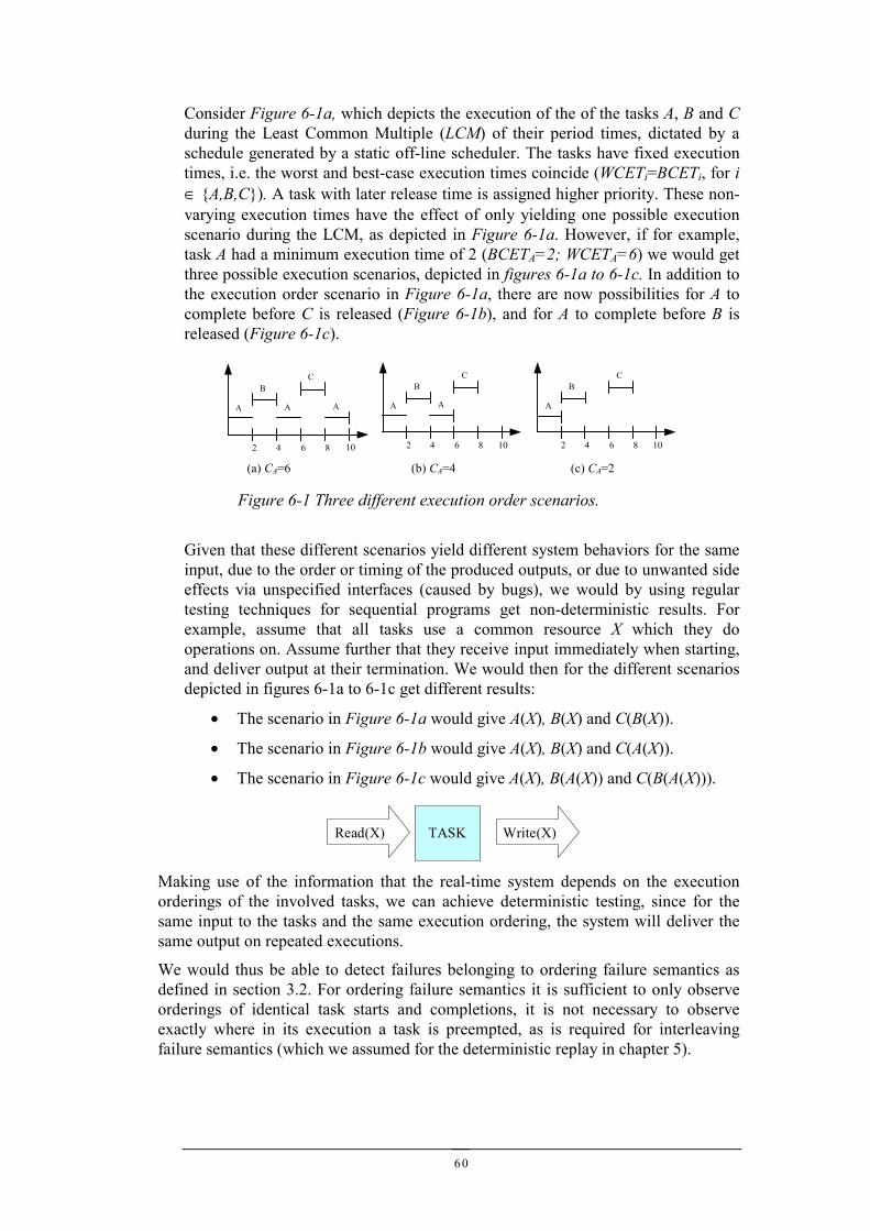
60

Consider Figure 6-1a, which depicts the execution of the of the tasks A, B and Cduring the Least Common Multiple (LCM) of their period times, dictated by aschedule generated by a static off-line scheduler. The tasks have fixed executiontimes, i.e. the worst and best-case execution times coincide (WCETi=BCETi, for i∈ {A,B,C}). A task with later release time is assigned higher priority. These non-varying execution times have the effect of only yielding one possible executionscenario during the LCM, as depicted in Figure 6-1a. However, if for example,task A had a minimum execution time of 2 (BCETA=2; WCETA=6) we would getthree possible execution scenarios, depicted in figures 6-1a to 6-1c. In addition tothe execution order scenario in Figure 6-1a, there are now possibilities for A tocomplete before C is released (Figure 6-1b), and for A to complete before B isreleased (Figure 6-1c).

Given that these different scenarios yield different system behaviors for the sameinput, due to the order or timing of the produced outputs, or due to unwanted sideeffects via unspecified interfaces (caused by bugs), we would by using regulartesting techniques for sequential programs get non-deterministic results. Forexample, assume that all tasks use a common resource X which they dooperations on. Assume further that they receive input immediately when starting,and deliver output at their termination. We would then for the different scenariosdepicted in figures 6-1a to 6-1c get different results:

• The scenario in Figure 6-1a would give A(X), B(X) and C(B(X)).

• The scenario in Figure 6-1b would give A(X), B(X) and C(A(X)).

• The scenario in Figure 6-1c would give A(X), B(A(X)) and C(B(A(X))).

Making use of the information that the real-time system depends on the executionorderings of the involved tasks, we can achieve deterministic testing, since for thesame input to the tasks and the same execution ordering, the system will deliver thesame output on repeated executions.

We would thus be able to detect failures belonging to ordering failure semantics asdefined in section 3.2. For ordering failure semantics it is sufficient to only observeorderings of identical task starts and completions, it is not necessary to observeexactly where in its execution a task is preempted, as is required for interleavingfailure semantics (which we assumed for the deterministic replay in chapter 5).

Figure 6-1 Three different execution order scenarios.

A A A

BC

2 4 6 8

A A

BC

2 4 6 8 1010

A

BC

2 4 6 8 10

(a) CA=6 (b) CA=4 (c) CA=2

TASKRead(X) Write(X)

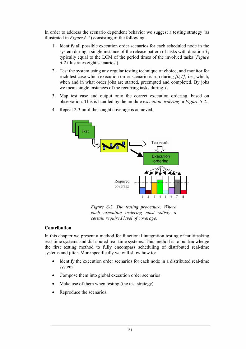
61

In order to address the scenario dependent behavior we suggest a testing strategy (asillustrated in Figure 6-2) consisting of the following:

1. Identify all possible execution order scenarios for each scheduled node in thesystem during a single instance of the release pattern of tasks with duration T;typically equal to the LCM of the period times of the involved tasks (Figure6-2 illustrates eight scenarios.)

2. Test the system using any regular testing technique of choice, and monitor foreach test case which execution order scenario is run during [0,T], i.e., which,when and in what order jobs are started, preempted and completed. By jobswe mean single instances of the recurring tasks during T.

3. Map test case and output onto the correct execution ordering, based onobservation. This is handled by the module execution ordering in Figure 6-2.

4. Repeat 2-3 until the sought coverage is achieved.

Contribution

In this chapter we present a method for functional integration testing of multitaskingreal-time systems and distributed real-time systems: This method is to our knowledgethe first testing method to fully encompass scheduling of distributed real-timesystems and jitter. More specifically we will show how to:

• Identify the execution order scenarios for each node in a distributed real-timesystem

• Compose them into global execution order scenarios

• Make use of them when testing (the test strategy)

• Reproduce the scenarios.

Figure 6-2. The testing procedure. Whereeach execution ordering must satisfy acertain required level of coverage.

Test result

Executionordering

1 2 3 4 5 6 7 8

Requiredcoverage

Test

62

6.1 The system modelWe refine the original system model from chapter 3 to encompass a distributedsystem consisting of a set of nodes, which communicate via a temporallypredictable broadcast network, i.e. upper and lower bounds on communicationlatencies are known or can be calculated [50][110]. Each node is a self sufficientcomputing element with CPU, memory, network access, a local clock and I/Ounits for sampling and actuation of the external system. We further assume theexistence of a global synchronized time base [51][27] with a known precision δ,meaning that no two nodes in the system have local clocks differing by more thanδ.

We further refine the original system model by assuming that the software thatruns on the distributed system consists of a set of concurrent tasks,communicating by message passing. Functionally related and cooperating tasks,e.g., sample-calculate-actuate loops in control systems, are defined astransactions. The relationship between the cooperating tasks with respect toprecedence (execution order), interactions (data-flow), and a period time typicallydefine each transaction. The tasks are distributed over the nodes, typically withtransactions that span several nodes, and with more than one task on each node.All synchronization is resolved before run-time and therefore no action is neededto enforce synchronization in the actual program code. Different release times andpriorities guarantee mutual exclusion and precedence. The distributed system isglobally scheduled, which results in a set of specific schedules for each node. Atrun-time we need only synchronize the local clocks to fulfill the global schedule[50].

Task model

We assume a fairly general task model that includes both preemptive schedulingof statically generated schedules [117] and fixed priority scheduling of strictlyperiodic tasks [4][75]:

• The system contains a set of jobs J, i.e. invocations of tasks, which arereleased in a time interval [t, t+TMAX], where TMAX is typically equal to theLeast Common Multiple (LCM) of the involved tasks period times, and tis an idle point within the time interval [0, TMAX] where no job isexecuting. The existence of such an idle point, t, simplifies the modelsuch that it prevents temporal interference between successive TMAX

intervals. To simplify the presentation we will henceforth assume an idlepoint at 0 for all participating nodes.

• Each job j∈ J has a release time rj, worst case execution time (WCETj),best case execution time (BCETj), a deadline Dj and a priority pj. Jrepresents one instance of a recurring pattern of job executions withperiod TMAX, i.e., job j will be released at time rj, rj+ TMAX, rj+ 2TMAX, etc.

• The system is preemptive and jobs may have identical release-times.

Related to the task model we assume that the tasks may have functional andtemporal side effects due to preemption, message passing and shared memory.Furthermore, we assume that data is sent at the termination of the sending task(not during its execution), and that received data is available when tasks start (andis made private in an atomic first operation of the task) [108][26][54].

63

Fault hypothesis

Note that, although synchronization is resolved by the off-line selection of releasetimes and priorities, we cannot dismiss unwanted synchronization side effects.The schedule design can be erroneous, or the assumptions about the executiontimes might not be accurate due to poor execution time estimates, or simply dueto design and coding errors.

Inter-task communication is restricted to the beginning and end of task execution,and therefore we can regard the interval of execution for tasks as atomic. Withrespect to access to shared resources, such as shared memory and I/O interfaces,the atomicity assumption is only valid if synchronization and mutual exclusioncan be guaranteed.

The fault hypothesis is thus:

Errors can only occur due to erroneous outputs and inputs to jobs, and/ordue to synchronization errors, i.e., jobs can only interfere via specifiedinteractions. This hypothesis corresponds to ordering failure semantics asdefined in section 3.2.

One way to guarantee the fault hypothesis in a shared memory system is to makeuse of hardware memory protection schemes, or during design eliminate orminimize shared resources using wait-free and lock-free communication[108][52][13].

6.2 Execution order analysisIn this section we present a method for identifying all the possible orders ofexecution for sets of jobs conforming to the task model introduced in section 6.1.We will also show how the model and analysis can be extended to accommodatefor interrupt interference and multiple nodes in a distributed system byconsidering clock-synchronization effects, parallel executions, and varyingcommunication latencies.

6.2.1 Execution OrderingsIn identifying the execution orderings of a job set we will only consider thefollowing major events of job executions:

• The start of execution of a job, i.e., when the first instruction of a job isexecuted. We will use S(J) to denote the set of start points for the jobs in ajob set J; S(J) ⊆ J × [0, TMAX] × J ∪{_}, that is S(J) is the set of triples(j1, time, j2), where j2 is the (lower priority) job that is preempted by thestart of j1 at time, or possibly “_” if no such job exists.

• The end of execution of a job, i.e., when the last instruction of a job isexecuted. We will use E(J) to denote the set of end points (terminationpoints) for jobs in a job set J; E(J) ⊆ J × [0, TMAX] × J ∪{_}, that is E(J) isa set of triples (j1, time, j2), where j2 is the (lower priority) job thatresumes its execution at the termination of j1, or possibly “_” if no suchjob exists.

64

We will now define an execution to be a sequence of job starts and jobterminations, using the additional notation that

• ev denotes an event, and Ev a set of events.

• ev.t denotes the time of the event ev,

• Ev\I denotes the set of events in Ev that occur in the time interval I,

• Prec(Ev, t) is the event in Ev that occurred most recently at time t(including an event that occurs at t).

• Nxt(Ev, t) denotes the next event in Ev after time t.

• First(Ev) and Last(Ev) denote the first and last event in Ev, respectively.

Definition 6-1. An Execution of a job set J is a set of events X ⊆ S(J) ∪ E(J),such that

1) For each j∈J, there is exactly one start and termination event in X,denoted s(j,X) and e(j,X) respectively, and s(j,X) precedes e(j,X), i.e.s(j,X).t ≤ e(j,X).t, where s(j,X) ∈ S(J) and e(j,X) ∈ E(J).

2) For each (j1, t, j2) ∈ S(J), pj1 > pj2, i.e., jobs are only preempted by higherpriority jobs.

3) For each j∈J, s(j,X).t ≥ rj, i.e., jobs may only start to execute after beingreleased.

4) After its release, the start of a job may only be delayed by intervals ofexecutions of higher priority jobs, i.e., using the convention thatX\[j.t, j.t)=∅.

For each job j∈J each event ev∈X\[Prec(X,rj).t, s(j,X).t) is either

• A start of the execution of a higher priority job, i.e. ev = s(j’, X) andpj’>pj

• A job termination, at which a higher priority job resumes itsexecution, i.e., ev = (j’, t, j”), where pj”>pj

5) The sum of execution intervals of a job j∈J is in the range[BCET(j), WCET(j)], i.e.,

BCET(j) ≤ ≤ WCET(j)

That is, we are summing up the intervals in which j starts or resumes itsexecution.

We will use EXt(J) to denote the set of executions of the job set J. Intuitively,EXt(J) denotes the set of possible executions of the job set J within [0,TMAX].Assuming a dense time domain EXt(J) is only finite if BCET(j)= WCET(j) for allj∈J. However, if we disregard the exact timing of events and only consider theordering of events we obtain a finite set of execution orderings for any finite jobset J.

Using ev{x/t} to denote an event ev with the time element t replaced by theundefined element “x”, we can formally define the set of execution orderingsEXo(J) as follows:

∑∈∪∈ )}(),,'(|),,'({ X)}{s(j, ev

ev.t -ev.t).t Nxt(X,JEjtjjtj

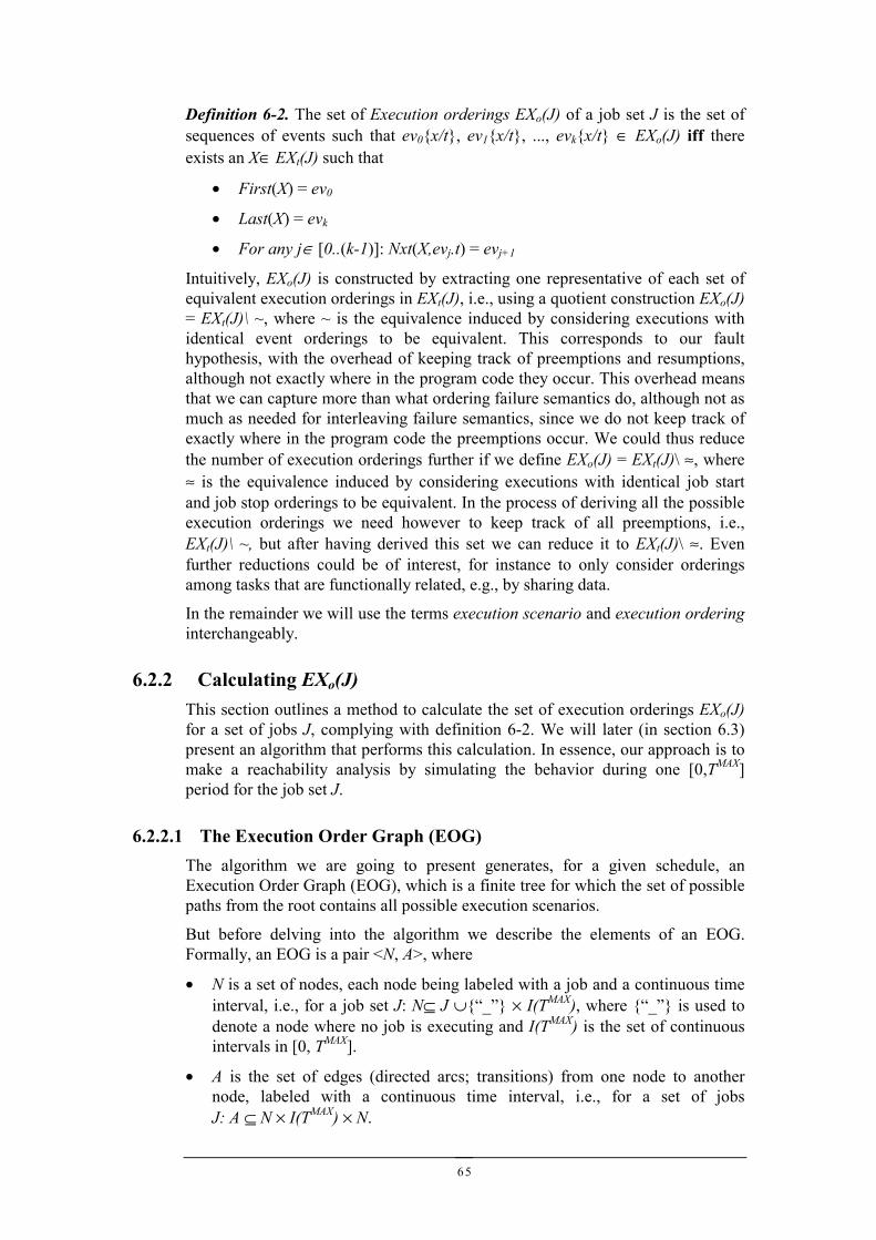
65

Definition 6-2. The set of Execution orderings EXo(J) of a job set J is the set ofsequences of events such that ev0{x/t}, ev1{x/t}, ..., evk{x/t} ∈ EXo(J) iff thereexists an X∈ EXt(J) such that

• First(X) = ev0

• Last(X) = evk

• For any j∈ [0..(k-1)]: Nxt(X,evj.t) = evj+1

Intuitively, EXo(J) is constructed by extracting one representative of each set ofequivalent execution orderings in EXt(J), i.e., using a quotient construction EXo(J)= EXt(J)\ ~, where ~ is the equivalence induced by considering executions withidentical event orderings to be equivalent. This corresponds to our faulthypothesis, with the overhead of keeping track of preemptions and resumptions,although not exactly where in the program code they occur. This overhead meansthat we can capture more than what ordering failure semantics do, although not asmuch as needed for interleaving failure semantics, since we do not keep track ofexactly where in the program code the preemptions occur. We could thus reducethe number of execution orderings further if we define EXo(J) = EXt(J)\ ≈, where≈ is the equivalence induced by considering executions with identical job startand job stop orderings to be equivalent. In the process of deriving all the possibleexecution orderings we need however to keep track of all preemptions, i.e.,EXt(J)\ ~, but after having derived this set we can reduce it to EXt(J)\ ≈. Evenfurther reductions could be of interest, for instance to only consider orderingsamong tasks that are functionally related, e.g., by sharing data.

In the remainder we will use the terms execution scenario and execution orderinginterchangeably.

6.2.2 Calculating EXo(J)This section outlines a method to calculate the set of execution orderings EXo(J)for a set of jobs J, complying with definition 6-2. We will later (in section 6.3)present an algorithm that performs this calculation. In essence, our approach is tomake a reachability analysis by simulating the behavior during one [0,TMAX]period for the job set J.

6.2.2.1 The Execution Order Graph (EOG)The algorithm we are going to present generates, for a given schedule, anExecution Order Graph (EOG), which is a finite tree for which the set of possiblepaths from the root contains all possible execution scenarios.

But before delving into the algorithm we describe the elements of an EOG.Formally, an EOG is a pair <N, A>, where

• N is a set of nodes, each node being labeled with a job and a continuous timeinterval, i.e., for a job set J: N⊆ J ∪{“_”} × I(TMAX), where {“_”} is used todenote a node where no job is executing and I(TMAX) is the set of continuousintervals in [0, TMAX].

• A is the set of edges (directed arcs; transitions) from one node to anothernode, labeled with a continuous time interval, i.e., for a set of jobsJ: A ⊆ N × I(TMAX) × N.

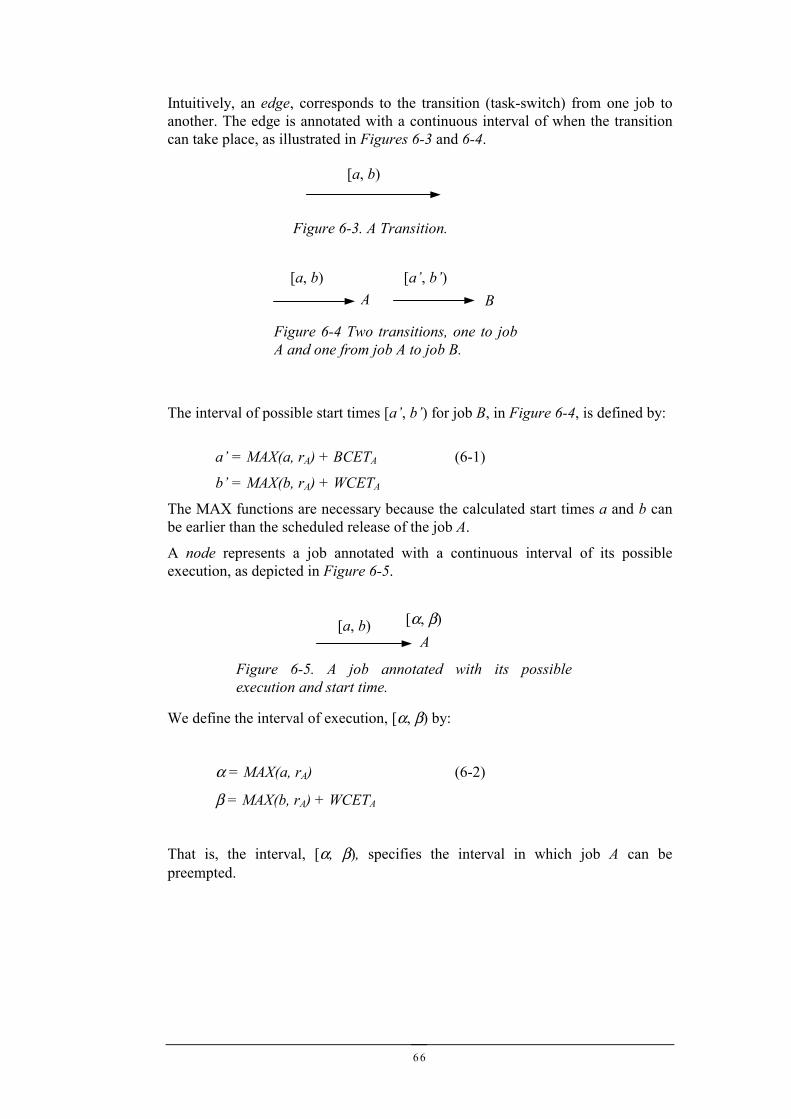
66

Intuitively, an edge, corresponds to the transition (task-switch) from one job toanother. The edge is annotated with a continuous interval of when the transitioncan take place, as illustrated in Figures 6-3 and 6-4.

The interval of possible start times [a’, b’) for job B, in Figure 6-4, is defined by:

a’ = MAX(a, rA) + BCETA (6-1)

b’ = MAX(b, rA) + WCETA

The MAX functions are necessary because the calculated start times a and b canbe earlier than the scheduled release of the job A.

A node represents a job annotated with a continuous interval of its possibleexecution, as depicted in Figure 6-5.

We define the interval of execution, [α, β) by:

α = MAX(a, rA) (6-2)

β = MAX(b, rA) + WCETA

That is, the interval, [α, β), specifies the interval in which job A can bepreempted.

[a, b)

Figure 6-3. A Transition.

[a, b)A

[a’, b’)B

Figure 6-4 Two transitions, one to jobA and one from job A to job B.

[α, β)A

[a, b)

Figure 6-5. A job annotated with its possibleexecution and start time.

67

From each node in the execution ordering graph there can be one or moretransitions, representing one of four different situations:

1) The job is the last job scheduled in this branch of the tree. In this case thetransition is labeled with the interval of finishing times for the node, andhas the empty job “_” as destination node, as exemplified in Figure 6-6.

2) The job has a WCET such that it definitely completes before the release ofany higher priority job. In this case we have two situations:

a) Normal situation. One single outgoing transition labeled with theinterval of finishing times for the job, [a’, b’). Exemplified by (1) inFigure 6-6.

b) Special case. If a higher priority job is immediately succeeding at[b’,b’] while b’ > a’, and there are lower priority jobs ready, or madeready during [α,β) then we have two possible transitions: One branchlabeled with the interval of finishing times [a’,b’) representing theimmediate succession of a lower priority job, and one labeled [b’, b’)representing the completion immediately before the release of thehigher priority job. Exemplified by (2) in Figure 6-6.

3) The job has a BCET such that it definitely is preempted by another job. Inthis case there is a single outgoing transition labeled with the preemptiontime t, expressed by the interval [t, t], as exemplified by (3) in Figure 6-6.

4) The job has a BCET and WCET such that it may either complete or bepreempted before any preempting job is released. In this case there can betwo or three possible outgoing edges depending on if there are any lowerpriority jobs ready. One branch representing the preemption, labeled withthe preemption time [t, t], and depending on if there are any lower priorityjobs ready for execution we have two more transition situations:

a) No jobs ready. Then there is one branch labeled [a’, t) representingthe possible completion prior to the release of the higher priority job.Exemplified by (4) in Figure 6-6.

b) Lower priority jobs ready. If β > α then there is one branch labeled[a’, t) representing the immediate succession of a lower priority job,and one labeled [t, t) representing the completion immediately beforethe release of the preempting job. Exemplified by (5) in Figure 6-6.

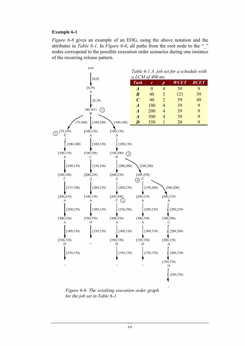
68

Example 6-1

Figure 6-6 gives an example of an EOG, using the above notation and theattributes in Table 6-1. In Figure 6-6, all paths from the root node to the “_”nodes correspond to the possible execution order scenarios during one instanceof the recurring release pattern.

Figure 6-6. The resulting execution order graphfor the job set in Table 6-1.

3

2

4

1

5

Table 6-1 A job set for a schedule witha LCM of 400 ms.Task r p WCET BCET

A 0 4 39 9B 40 3 121 39C 40 2 59 49A 100 4 39 9A 200 4 39 9A 300 4 39 9D 350 1 20 9

69

6.3 The EOG algorithmHere we will define the algorithm for generating the EOG (Figure 6-7).Essentially, the algorithm simulates the behavior of a strictly periodic fixedpriority preemptive real-time kernel, complying with the previously defined taskmodel and EOG primitives. In defining the algorithm we use the followingauxiliary functions and data structures:

1) rdy – the set of jobs ready to execute.2) Next_release(I) – returns the earliest release time of a job j∈J within the

interval I. If no such job exists then ∞ is returned . Also, we will use I.land I.r to denote the extremes of I.

3) P(t) – Returns the highest priority of the jobs that are released at time t.Returns -1 if t = ∞.

4) Make_ready(t, rdy) – adds all jobs that are released at time t to rdy.Returns ∅ if t=∞, else the set.

5) X(rdy) extracts the job with highest priority in rdy.6) Arc(n, I, n’) creates an edge from node n to node n’ and labels it with the

time interval I.7) Make_node(j, XI) creates a node and labels it with the execution interval

XI and the id of job j.The execution order graph for a set of jobs J is generated by a call Eog(ROOT,{}, [0, 0], [0, TMAX]), i.e., with a root node, an empty ready set, and the initialrelease interval [0,0], plus the considered interval [0, TMAX].

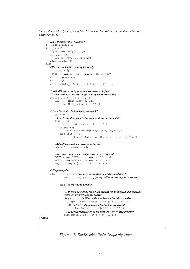
70

// n- previous node, rdy- set of ready jobs, RI – release interval, SI – the considered interval.Eog(n, rdy, RI, SI){

//When is the next job(s) released?t = Next_release(SI)

if (rdy = ∅)rdy = Make_ready(t, rdy)

if( rdy ≠ ∅)Eog (n, rdy, RI, (t,SI.r] )

else Arc(n, RI, _ )else

//Extract the highest priority job in rdy.T = X(rdy)

[α,β) = [max(rT, RI.l), max(rT, RI.l)+WCETT)

a’ = α + BCETTb’ = βn’ = Make_node(T, [α,β) ) Arc(n, RI, n’)

// Add all lower priority jobs that are released beforeT's termination, or before a high priority job is preempting T.while((t < β) ∧ (P(t) < pT))

rdy = Make_ready(t, rdy)t = Next_release((t, SI.r])

// Does the next scheduled job preempt T?if((pT < P(t)) ∧ (t < β))

// Can T complete prior to the release of the next job at t?if(t > a’)

Eog ( n’, rdy, [a’,t), [t,SI.r] )

if(rdy ≠ ∅)Eog(n’,Make_ready(t,rdy),[t,t),(t,SI.r])

else if(t = a’)Eog(n’, Make_ready(t, rdy), [t,t), (t,SI.r])

//Add all jobs that are released at time t.rdy = Make_ready(t, rdy)

//Best and worst case execution prior to preemption?BCETT = max(BCETT - (t–(max(rT, RI.l)),0)WCETT = max(WCETT - (t–(max(rT, RI.r)),0)Eog( n’, rdy + {T}, [t,t], (t,SI.r])

// No preemptionelse if(t = ∞ ) //Have we come to the end of the simulation?

Eog(n’, rdy, [a’,b’),[∞,∞]) //Yes, no more jobs to execute

else // More jobs to execute

//Is there a possibility for a high priority job to succeed immediately,while low priority jobs are ready?if(rdy ≠ ∅ ∧ t = β) //Yes, make one branch for this transition

Eog(n’, Make_ready(t, rdy),[t,t),(t,SI.r])

if(a’ ≠ b’) //And one branch for the low priority jobelse Eog(n’, rdy, [a’,b’),[t, SI.r))

// The regular succession of the next job (low or high priority)else Eog(n’, rdy, [a’,b’),[t, SI.r))

}//End

Figure 6-7. The Exection Order Graph algorithm.

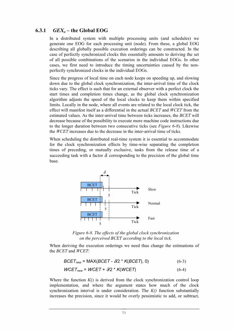
71

6.3.1 GEXo – the Global EOGIn a distributed system with multiple processing units (and schedules) wegenerate one EOG for each processing unit (node). From these, a global EOGdescribing all globally possible execution orderings can be constructed. In thecase of perfectly synchronized clocks this essentially amounts to deriving the setof all possible combinations of the scenarios in the individual EOGs. In othercases, we first need to introduce the timing uncertainties caused by the non-perfectly synchronized clocks in the individual EOGs.

Since the progress of local time on each node keeps on speeding up, and slowingdown due to the global clock synchronization, the inter-arrival time of the clockticks vary. The effect is such that for an external observer with a perfect clock thestart times and completion times change, as the global clock synchronizationalgorithm adjusts the speed of the local clocks to keep them within specifiedlimits. Locally in the node, where all events are related to the local clock tick, theeffect will manifest itself as a differential in the actual BCET and WCET from theestimated values. As the inter-arrival time between ticks increases, the BCET willdecrease because of the possibility to execute more machine code instructions dueto the longer duration between two consecutive ticks (see Figure 6-8). Likewisethe WCET increases due to the decrease in the inter-arrival time of ticks.

When scheduling the distributed real-time system it is essential to accommodatefor the clock synchronization effects by time-wise separating the completiontimes of preceding, or mutually exclusive, tasks from the release time of asucceeding task with a factor δ, corresponding to the precision of the global timebase.

When deriving the execution orderings we need thus change the estimations ofthe BCET and WCET:

BCETnew = MAX(BCET - δ/2 * K(BCET), 0) (6-3)

WCETnew = WCET + δ/2 * K(WCET) (6-4)

Where the function K() is derived from the clock synchronization control loopimplementation, and where the argument states how much of the clocksynchronization interval is under consideration. The K() function substantiallyincreases the precision, since it would be overly pessimistic to add, or subtract,

BCET

Tick

5 Tick

Slow

NormalBCET

5 TickFast

BCET

5

δ

Figure 6-8. The effects of the global clock synchronizationon the perceived BCET according to the local tick.

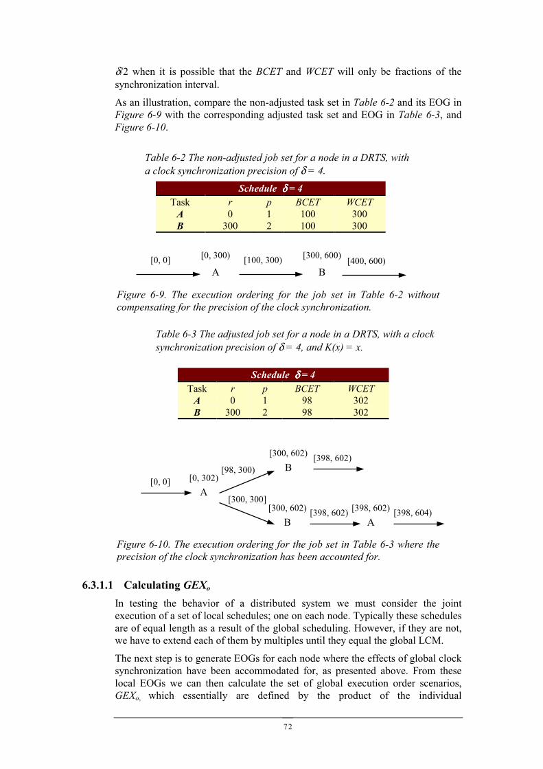
72

δ/2 when it is possible that the BCET and WCET will only be fractions of thesynchronization interval.

As an illustration, compare the non-adjusted task set in Table 6-2 and its EOG inFigure 6-9 with the corresponding adjusted task set and EOG in Table 6-3, andFigure 6-10.

6.3.1.1 Calculating GEXo

In testing the behavior of a distributed system we must consider the jointexecution of a set of local schedules; one on each node. Typically these schedulesare of equal length as a result of the global scheduling. However, if they are not,we have to extend each of them by multiples until they equal the global LCM.

The next step is to generate EOGs for each node where the effects of global clocksynchronization have been accommodated for, as presented above. From theselocal EOGs we can then calculate the set of global execution order scenarios,GEXo, which essentially are defined by the product of the individual

Schedule δδδδ = 4Task r p BCET WCET

A 0 1 98 302B 300 2 98 302

Table 6-3 The adjusted job set for a node in a DRTS, with a clocksynchronization precision of δ = 4, and K(x) = x.

[98, 300)[0, 0]

A[0, 302)

B[300, 602) [398, 602)

B[300, 602) [398, 602)

A[398, 602) [398, 604)

[300, 300]

Figure 6-10. The execution ordering for the job set in Table 6-3 where theprecision of the clock synchronization has been accounted for.

Schedule δδδδ = 4Task r p BCET WCET

A 0 1 100 300B 300 2 100 300

Table 6-2 The non-adjusted job set for a node in a DRTS, witha clock synchronization precision of δ = 4.

[0, 0]A

[0, 300) [100, 300)B

[300, 600) [400, 600)

Figure 6-9. The execution ordering for the job set in Table 6-2 withoutcompensating for the precision of the clock synchronization.

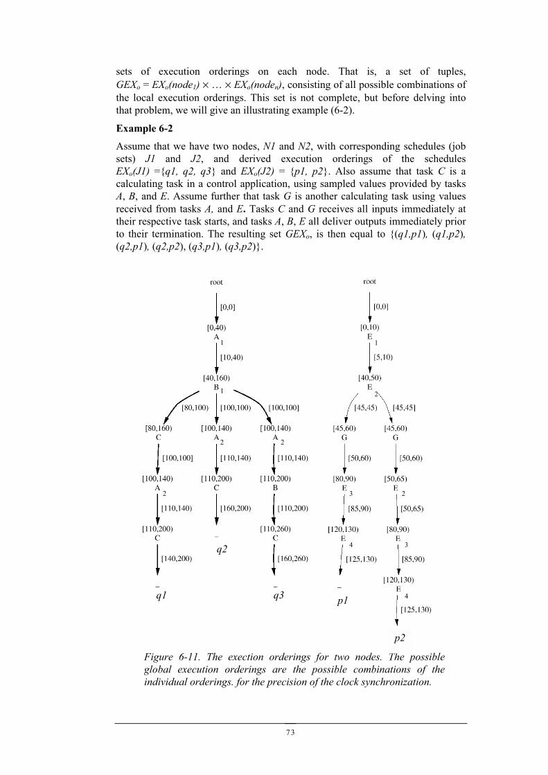
73

sets of execution orderings on each node. That is, a set of tuples,GEXo = EXo(node1) × … × EXo(noden), consisting of all possible combinations ofthe local execution orderings. This set is not complete, but before delving intothat problem, we will give an illustrating example (6-2).

Example 6-2

Assume that we have two nodes, N1 and N2, with corresponding schedules (jobsets) J1 and J2, and derived execution orderings of the schedulesEXo(J1) ={q1, q2, q3} and EXo(J2) = {p1, p2}. Also assume that task C is acalculating task in a control application, using sampled values provided by tasksA, B, and E. Assume further that task G is another calculating task using valuesreceived from tasks A, and E. Tasks C and G receives all inputs immediately attheir respective task starts, and tasks A, B, E all deliver outputs immediately priorto their termination. The resulting set GEXo, is then equal to {(q1,p1), (q1,p2),(q2,p1), (q2,p2), (q3,p1), (q3,p2)}.

Figure 6-11. The exection orderings for two nodes. The possibleglobal execution orderings are the possible combinations of theindividual orderings. for the precision of the clock synchronization.

q1

q2

1

1

2 2

2

p1

2

1

3 2

34

4q3

p2

74

The set GEXo = {(q1,p1), (q1,p2), (q2,p1), (q2,p2), (q3,p1), (q3,p2)}, is howevernot complete. Analyzing the data dependencies between task C on node N1 andtask E on node N2, we see that task C can receive data from different instances oftask E. The same goes for task G, on node N2, with respect to task A, on node N1.

For example, during the global scenario (q1, p1), task C has a varying start timeof [80,100) and within that interval task instance E3, has a completion interval of[85,90]. This means, if we assume communication latencies in the interval [3,6),that task C can receive data from task instance E2 or E3. In order to differentiatebetween these scenarios we should therefore substitute the global ordering (q1,p1)with the set (q1:C(E2), p1) and (q1:C(E3), p1). Where “(q1:C(E2), p1)” meansthat during scenario (q1,p1), task C receives data from task E, and that theoriginating instance of task E is of significance.

For task G, assuming the same communication latencies, this means that it canreceive data from task instance A0 or A1, yielding a new set of scenarios, e.g.,scenario (q1,p1) is substituted with (q1, p1:G(A0)) and (q1, p1:G(A1)). Thesetransformations necessitates that we, in addition to recording the executionorderings during runtime, need to tag all data such that we can differentiatebetween different instances, corresponding to different originators.

From the viewpoint of node N1 the transformed set would look like:{(q1:C(E2), p1), (q1:C(E3), p1), (q1:C(E2), p2), (q1:C(E3), p2),

(q2:C(E3), p1), (q2:C(E4), p1), (q2:C(E3), p2), (q2:C(E4), p2),

(q3:C(E3), p1), (q3:C(E4), p1), (q3:C(E3), p2), (q3:C(E4), p2)}.

From the viewpoint of node N2 the transformed set would look like:{(q1, p1:G(A0)), (q1, p1:G(A1)), (q1, p2:G(A0)), (q1, p2:G(A1)),

(q2, p1:G(A0)), (q2, p1:G(A1)), (q2, p2:G(A0)), (q2, p2:G(A1)),

(q3, p1:G(A0)), (q3, p1:G(A1)), (q3, p2:G(A0)), (q3, p2:G(A1))}

That is, the new transformed execution orderings are:• EXo(J1)={q1:C(E2), q1:C(E3), q2:C(E3), q2:C(E4), q3:C(E3), q3:C(E4)}

• EXo(J2)={ p1:G(A0), p1:G(A1), p2:G(A0), p2:G(A1)}

The new transformed set GEXo = EXo(J1) × EXo(J2) becomes:{(q1:C(E2), p1:G(A0)), (q1:C(E3), p1:G(A0)), (q1:C(E2), p2:G(A0)), (q1:C(E3), p2:G(A0)),

(q2:C(E3), p1:G(A0)), (q2:C(E4), p1:G(A0)), (q2:C(E3), p2:G(A0)), (q2:C(E4), p2:G(A0)),

(q3:C(E3), p1:G(A0)), (q3:C(E4), p1:G(A0)), (q3:C(E3), p2:G(A0)), (q3:C(E4), p2:G(A0)),

(q1:C(E2), p1:G(A1)), (q1:C(E3), p1:G(A1)), (q1:C(E2), p2:G(A1)), (q1:C(E3), p2:G(A1)),

(q2:C(E3), p1:G(A1)), (q2:C(E4), p1:G(A1)), (q2:C(E3), p2:G(A1)), (q2:C(E4), p2:G(A1)),

(q3:C(E3), p1:G(A1)), (q3:C(E4), p1:G(A1)), (q3:C(E3), p2:G(A1)), (q3:C(E4), p2:G(A1)}.

75

6.3.1.2 GEXo data dependency transformationWe will now more formally define these transformations. Assume the followingauxiliary functions:

• Start(j), returns the interval of start times for job j, (task instance)

• Finish(j), returns the interval of finishing times for job j.

• ComLatency(i,j), returns the communication latency interval for data sentby job i to job j.

• Precede(j), returns the immediately preceding instance of the same task asjob j. Note that this may be a job from the previous LCM.

Data dependency transformation definition

We transform the local execution orderings, EXo(node), with respect to the set ofglobal execution orderings, GEXo = EXo(node1) × … × EXo(noden):

1. For each tupel l ∈ GEXo.2. For each ordering x∈ EXo(n), where x is an element in tupel l, and

where K(x) is the set of jobs in x consuming data originating from theset of jobs, P, belonging to the other execution ordering elements of l.3. For each job j ∈ K(x).

4. For each subset Pt ⊆ P representing different instances of thesame task producing data for job j.5. Let Q be the set of jobs in Pt with finishing times +

communication delays, in the start time interval of job j,i.e., Q={u | start(j) ∩ (Finish(u) + ComLatency(u,j))≠∅}The set can be ordered by earliest finishing time. We use qto denote the earliest job in Q.

6. If Q ≠ ∅ substitute x. That is,EXo(n) = EXo(n)\x + x: j(Precede(q)) + (∀u ∈ Q| x:j(u)).

7. Substitute all x:j(y) ∈ EXo(n) where j ∈ K(x) and y ∈ P such thatwe for the scenario x, construct a substitute of all possiblecombinations of {x:j(ym), x:j’(y’m’),…, x:j”(y”m”)} ⊆ EXo(n) forconsuming jobs, {j,…,j”} ⊆ K(x) not belonging to the same taskinstance, i.e., combinations x:j(ym):j’(y’m’):…:j”(y”m”) in order ofstart time for jobs consuming data produced byjobs {ym,…,y”m”} ⊆ P.

8. New transformed GEXo = EXo(node1) × … × EXo(noden)

Example 6-3

Assume the same system as in Example 6-2, where the initialGEXo = { (q1,p1) , (q1,p2), (q2,p1), (q2,p2) , (q3,p1), (q3,p2) }.

The first tupel would be l = (q1,p1), the consuming task set in scenario q1 wouldbe K(q1) = {C}, the producing set of jobs for K(q1) would be Pt=P={Eold,E1, E2,E3, E4}, and the set of jobs Q that has a chance of producing data for the sole jobin K(q1), C, is Q={ E2, E3}. We thus substitute q1with q1:C(E2) and q1:C(E3).

76

Likewise we can transform all sets:

• EXo(J1)={q1:C(E2), q1:C(E3), q2:C(E3), q2:C(E4), q3:C(E3), q3:C(E4)}

• EXo(J2)={ p1:G(A0), p1:G(A1), p2:G(A0), p2:G(A1)}

The transformed global execution ordering set GEXo = EXo(J1) × EXo(J2) ={(q1:C(E2), p1:G(A0)), (q1:C(E3), p1:G(A0)), (q1:C(E2), p2:G(A0)), (q1:C(E3), p2:G(A0)),

(q2:C(E3), p1:G(A0)), (q2:C(E4), p1:G(A0)), (q2:C(E3), p2:G(A0)), (q2:C(E4), p2:G(A0)),

(q3:C(E3), p1:G(A0)), (q3:C(E4), p1:G(A0)), (q3:C(E3), p2:G(A0)), (q3:C(E4), p2:G(A0)),

(q1:C(E2), p1:G(A1)), (q1:C(E3), p1:G(A1)), (q1:C(E2), p2:G(A1)), (q1:C(E3), p2:G(A1)),

(q2:C(E3), p1:G(A1)), (q2:C(E4), p1:G(A1)), (q2:C(E3), p2:G(A1)), (q2:C(E4), p2:G(A1)),

(q3:C(E3), p1:G(A1)), (q3:C(E4), p1:G(A1)), (q3:C(E3), p2:G(A1)), (q3:C(E4), p2:G(A1)}.

6.4 Towards systematic testingWe will now outline a method for deterministic integration testing of distributedreal-time systems, based on the identification of execution orderings, as presentedabove. This method is suitable if we want to address ordering failure semantics.We can use it for interleaving failure semantics also, although since we do notkeep track of the exact interleavings we cannot guarantee deterministic testing,only partial determinism (as defined in section 3.2.2).If we are only interested in addressing sequential failure semantics we can makeuse of regular unit testing [6], and regard each task as a sequential program.However, if we want to take into account the effects that the tasks may have oneach other, we need to do integration testing, and assume ordering failuresemantics. In any case, we assume that some method for testing of sequentialprograms is used.

6.4.1 AssumptionsIn order to perform integration testing of distributed real-time systems we requirethe following:

• A feasible global schedule, including probes that will remain in the targetsystem in order to eliminate the probe effect (as discussed in chapter 4).

• Kernel-probes on each node that monitors task-switches. This information issent to dedicated tasks (probe-tasks) that identify execution orderings fromthe task-switch information and correlate it to run test cases.

• A set of in-line probes that instrument tasks, as well as probe-nodes, whichoutput and collect significant information to determine if a test run wassuccessful or not. This also includes auxiliary outputs of tasks’ state if theykeep state between invocations.

• Control over, or at least a possibility to observe, the input data to the systemwith regard to contents, order, and timing.

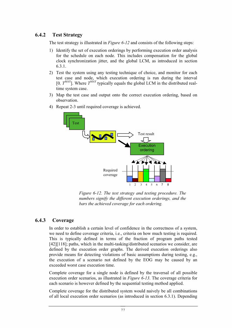
77

6.4.2 Test StrategyThe test strategy is illustrated in Figure 6-12 and consists of the following steps:

1) Identify the set of execution orderings by performing execution order analysisfor the schedule on each node. This includes compensation for the globalclock synchronization jitter, and the global LCM, as introduced in section6.3.1.

2) Test the system using any testing technique of choice, and monitor for eachtest case and node, which execution ordering is run during the interval[0, TMAX]. Where TMAX typically equals the global LCM in the distributed real-time system case.

3) Map the test case and output onto the correct execution ordering, based onobservation.

4) Repeat 2-3 until required coverage is achieved.

6.4.3 CoverageIn order to establish a certain level of confidence in the correctness of a system,we need to define coverage criteria, i.e., criteria on how much testing is required.This is typically defined in terms of the fraction of program paths tested[42][118]; paths, which in the multi-tasking/distributed scenarios we consider, aredefined by the execution order graphs. The derived execution orderings alsoprovide means for detecting violations of basic assumptions during testing, e.g.,the execution of a scenario not defined by the EOG may be caused by anexceeded worst case execution time.

Complete coverage for a single node is defined by the traversal of all possibleexecution order scenarios, as illustrated in Figure 6-13. The coverage criteria foreach scenario is however defined by the sequential testing method applied.

Complete coverage for the distributed system would naively be all combinationsof all local execution order scenarios (as introduced in section 6.3.1). Depending

Test result

Executionordering

1 2 3 4 5 6 7 8

Requiredcoverage

Figure 6-12. The test strategy and testing procedure. Thenumbers signify the different execution orderings, and thebars the achieved coverage for each ordering.

Test

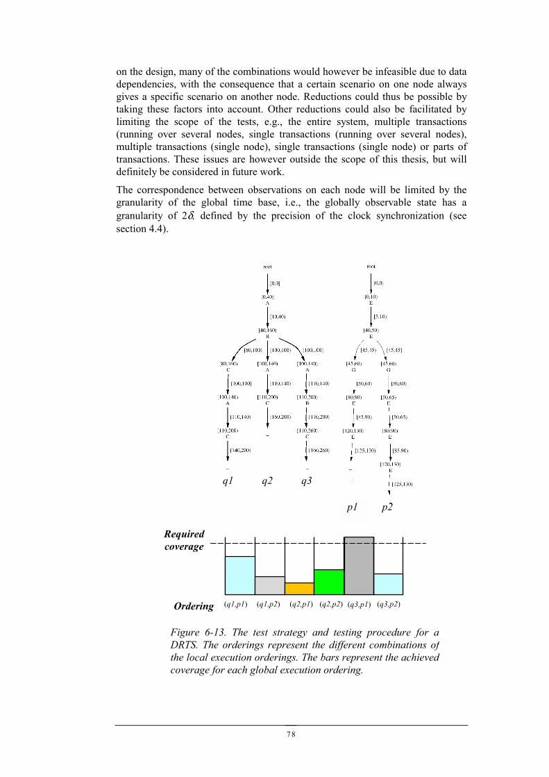
78

on the design, many of the combinations would however be infeasible due to datadependencies, with the consequence that a certain scenario on one node alwaysgives a specific scenario on another node. Reductions could thus be possible bytaking these factors into account. Other reductions could also be facilitated bylimiting the scope of the tests, e.g., the entire system, multiple transactions(running over several nodes, single transactions (running over several nodes),multiple transactions (single node), single transactions (single node) or parts oftransactions. These issues are however outside the scope of this thesis, but willdefinitely be considered in future work.

The correspondence between observations on each node will be limited by thegranularity of the global time base, i.e., the globally observable state has agranularity of 2δ, defined by the precision of the clock synchronization (seesection 4.4).

Figure 6-13. The test strategy and testing procedure for aDRTS. The orderings represent the different combinations ofthe local execution orderings. The bars represent the achievedcoverage for each global execution ordering.

q1 q2 pq3

p2p1

Requiredcoverage

Ordering (q3,p2)(q1,p1) (q1,p2) (q2,p2)(q2,p1) (q3,p1)

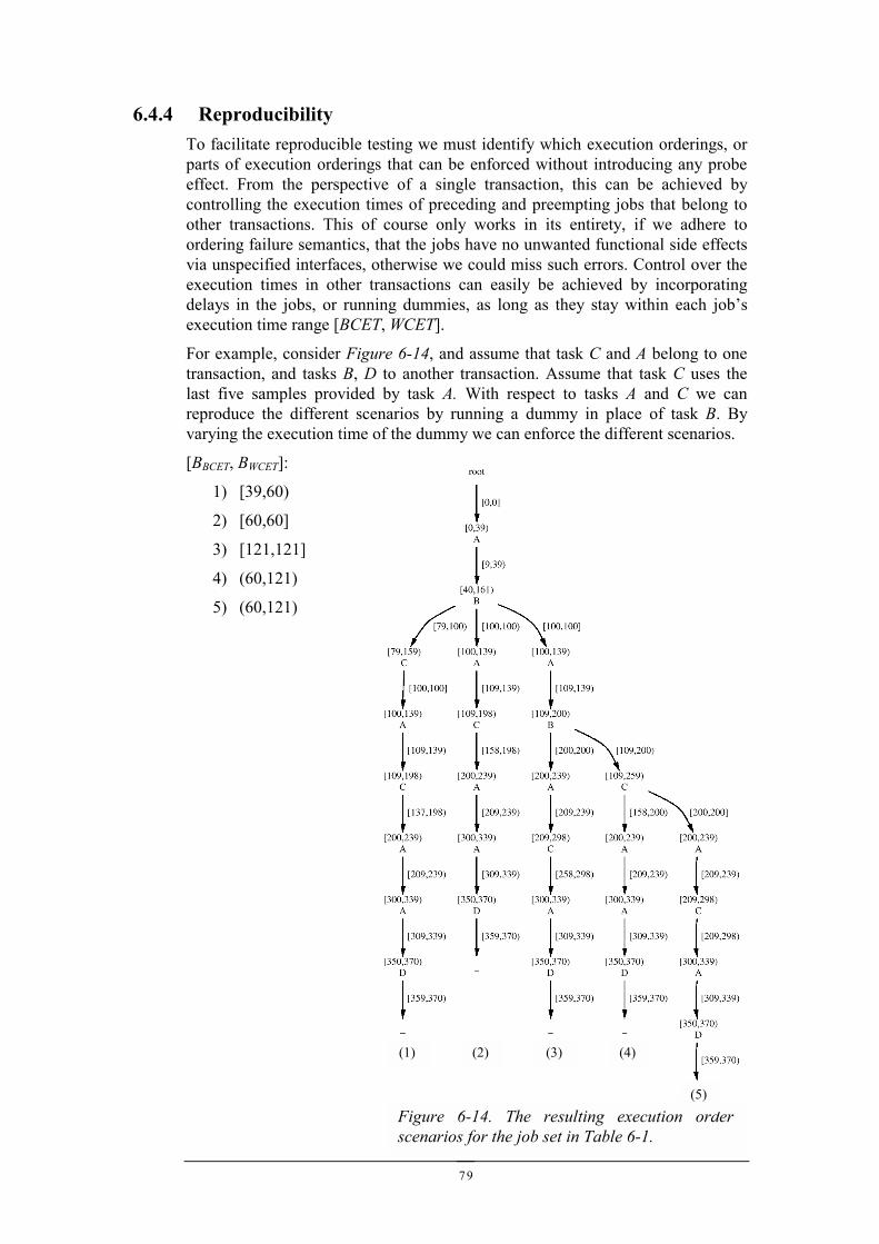
79

Figure 6-14. The resulting execution orderscenarios for the job set in Table 6-1.

(1) (2) (3) (4)

(5)

6.4.4 ReproducibilityTo facilitate reproducible testing we must identify which execution orderings, orparts of execution orderings that can be enforced without introducing any probeeffect. From the perspective of a single transaction, this can be achieved bycontrolling the execution times of preceding and preempting jobs that belong toother transactions. This of course only works in its entirety, if we adhere toordering failure semantics, that the jobs have no unwanted functional side effectsvia unspecified interfaces, otherwise we could miss such errors. Control over theexecution times in other transactions can easily be achieved by incorporatingdelays in the jobs, or running dummies, as long as they stay within each job’sexecution time range [BCET, WCET].

For example, consider Figure 6-14, and assume that task C and A belong to onetransaction, and tasks B, D to another transaction. Assume that task C uses thelast five samples provided by task A. With respect to tasks A and C we canreproduce the different scenarios by running a dummy in place of task B. Byvarying the execution time of the dummy we can enforce the different scenarios.

[BBCET, BWCET]:

1) [39,60)

2) [60,60]

3) [121,121]

4) (60,121)

5) (60,121)

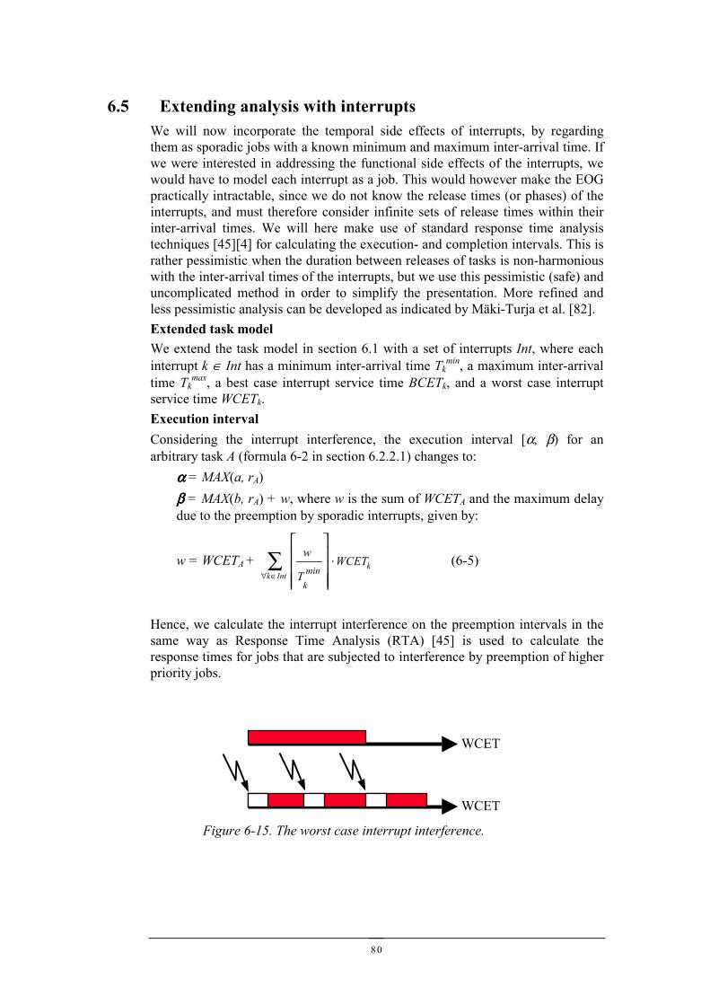
80

6.5 Extending analysis with interruptsWe will now incorporate the temporal side effects of interrupts, by regardingthem as sporadic jobs with a known minimum and maximum inter-arrival time. Ifwe were interested in addressing the functional side effects of the interrupts, wewould have to model each interrupt as a job. This would however make the EOGpractically intractable, since we do not know the release times (or phases) of theinterrupts, and must therefore consider infinite sets of release times within theirinter-arrival times. We will here make use of standard response time analysistechniques [45][4] for calculating the execution- and completion intervals. This israther pessimistic when the duration between releases of tasks is non-harmoniouswith the inter-arrival times of the interrupts, but we use this pessimistic (safe) anduncomplicated method in order to simplify the presentation. More refined andless pessimistic analysis can be developed as indicated by Mäki-Turja et al. [82].Extended task modelWe extend the task model in section 6.1 with a set of interrupts Int, where eachinterrupt k ∈ Int has a minimum inter-arrival time Tk

min, a maximum inter-arrivaltime Tk

max, a best case interrupt service time BCETk, and a worst case interruptservice time WCETk.Execution intervalConsidering the interrupt interference, the execution interval [α, β) for anarbitrary task A (formula 6-2 in section 6.2.2.1) changes to:

αααα = MAX(a, rA)ββββ = MAX(b, rA) + w, where w is the sum of WCETA and the maximum delaydue to the preemption by sporadic interrupts, given by:

w = WCETA + k Intk

WCETT

wmin

k

⋅

∑∈∀

(6-5)

Hence, we calculate the interrupt interference on the preemption intervals in thesame way as Response Time Analysis (RTA) [45] is used to calculate theresponse times for jobs that are subjected to interference by preemption of higherpriority jobs.

WCET

WCET

Figure 6-15. The worst case interrupt interference.

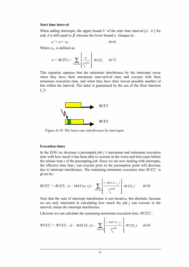
81

Start time interval

When adding interrupts, the upper bound b’ of the start time interval [a´, b’] fortask A is still equal to β, whereas the lower bound a’ changes to:

a’ = a + wa (6-6)

Where wa, is defined as:

w = BCETA + k Intk

BCETT

wmax

k

⋅

∑∈∀

(6-7)

This equation captures that the minimum interference by the interrupts occurwhen they have their maximum inter-arrival time and execute with theirminimum execution time, and when they have their lowest possible number ofhits within the interval. The latter is guaranteed by the use of the floor function( ).

Execution times

In the EOG we decrease a preempted job j’s maximum and minimum executiontime with how much it has been able to execute in the worst and best cases beforethe release time t of the preempting job. Since we are now dealing with interrupts,the effective time that j can execute prior to the preemption point will decreasedue to interrupt interference. The remaining minimum execution time BCETj’ isgiven by:

BCETj’ = BCETj - (t – MAX (a, rj) – kIntk

BCETT max

k

)jr (a, MAX- t⋅

∑

∈∀

) (6-8)

Note that the sum of interrupt interference is not iterative, but absolute, becausewe are only interested in calculating how much the job j can execute in theinterval, minus the interrupt interference.

Likewise we can calculate the remaining maximum execution time, WCETj’:

WCETj‘ = WCETj – (t – MAX (b, rj) – kIntk

WCETT min

k

)jr (b, MAX- t⋅

∑

∈∀

) (6-9)

BCET

BCET

Figure 6-16. The least case interference by interrupts.

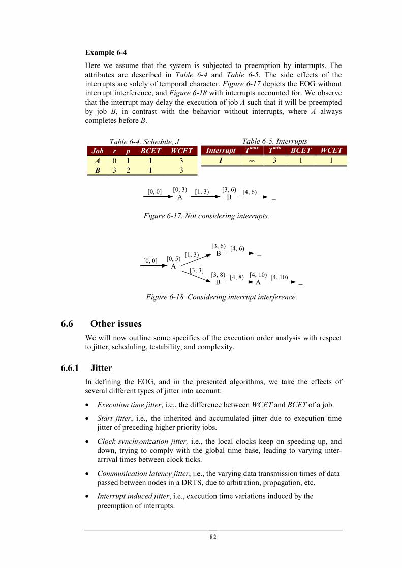
82

Example 6-4

Here we assume that the system is subjected to preemption by interrupts. Theattributes are described in Table 6-4 and Table 6-5. The side effects of theinterrupts are solely of temporal character. Figure 6-17 depicts the EOG withoutinterrupt interference, and Figure 6-18 with interrupts accounted for. We observethat the interrupt may delay the execution of job A such that it will be preemptedby job B, in contrast with the behavior without interrupts, where A alwayscompletes before B.

6.6 Other issuesWe will now outline some specifics of the execution order analysis with respectto jitter, scheduling, testability, and complexity.

6.6.1 JitterIn defining the EOG, and in the presented algorithms, we take the effects ofseveral different types of jitter into account:

• Execution time jitter, i.e., the difference between WCET and BCET of a job.

• Start jitter, i.e., the inherited and accumulated jitter due to execution timejitter of preceding higher priority jobs.

• Clock synchronization jitter, i.e., the local clocks keep on speeding up, anddown, trying to comply with the global time base, leading to varying inter-arrival times between clock ticks.

• Communication latency jitter, i.e., the varying data transmission times of datapassed between nodes in a DRTS, due to arbitration, propagation, etc.

• Interrupt induced jitter, i.e., execution time variations induced by thepreemption of interrupts.

[0, 0]A

[0, 3) [1, 3)B

[3, 6) [4, 6) _

Figure 6-17. Not considering interrupts.

[1, 3)[0, 0]

A[0, 5)

B[3, 6) [4, 6) _

B[3, 8) [4, 8)

A[4, 10) [4, 10) _

[3, 3]

Figure 6-18. Considering interrupt interference.

Table 6-4. Schedule, JJob r p BCET WCETA 0 1 1 3B 3 2 1 3

Table 6-5. InterruptsInterrupt Tmax Tmin BCET WCET

I ∞ 3 1 1

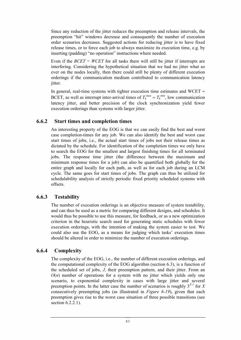
83

Since any reduction of the jitter reduces the preemption and release intervals, thepreemption “hit” windows decrease and consequently the number of executionorder scenarios decreases. Suggested actions for reducing jitter is to have fixedrelease times, or to force each job to always maximize its execution time, e.g. byinserting (padding) “no operation” instructions where needed.

Even if the BCET = WCET for all tasks there will still be jitter if interrupts areinterfering. Considering the hypothetical situation that we had no jitter what soever on the nodes locally, then there could still be plenty of different executionorderings if the communication medium contributed to communication latencyjitter.

In general, real-time systems with tighter execution time estimates and WCET ≈BCET, as well as interrupt inter-arrival times of Tk

max ≈ Tkmin, low communication

latency jitter, and better precision of the clock synchronization yield fewerexecution orderings than systems with larger jitter.

6.6.2 Start times and completion timesAn interesting property of the EOG is that we can easily find the best and worstcase completion-times for any job. We can also identify the best and worst casestart times of jobs, i.e., the actual start times of jobs not their release times asdictated by the schedule. For identification of the completion times we only haveto search the EOG for the smallest and largest finishing times for all terminatedjobs. The response time jitter (the difference between the maximum andminimum response times for a job) can also be quantified both globally for theentire graph and locally for each path, as well as for each job during an LCMcycle. The same goes for start times of jobs. The graph can thus be utilized forschedulability analysis of strictly periodic fixed priority scheduled systems withoffsets.

6.6.3 TestabilityThe number of execution orderings is an objective measure of system testability,and can thus be used as a metric for comparing different designs, and schedules. Itwould thus be possible to use this measure, for feedback, or as a new optimizationcriterion in the heuristic search used for generating static schedules with fewerexecution orderings, with the intention of making the system easier to test. Wecould also use the EOG, as a means for judging which tasks’ execution timesshould be altered in order to minimize the number of execution orderings.

6.6.4 ComplexityThe complexity of the EOG, i.e., the number of different execution orderings, andthe computational complexity of the EOG algorithm (section 6.3), is a function ofthe scheduled set of jobs, J, their preemption pattern, and their jitter. From anO(n) number of operations for a system with no jitter which yields only onescenario, to exponential complexity in cases with large jitter and severalpreemption points. In the latter case the number of scenarios is roughly 3X-1 for Xconsecutively preempting jobs (as illustrated in Figure 6-19), given that eachpreemption gives rise to the worst case situation of three possible transitions (seesection 6.2.2.1).

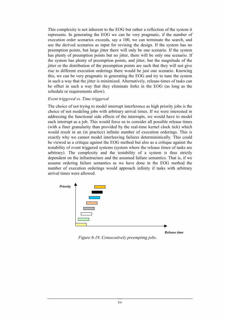
84

This complexity is not inherent to the EOG but rather a reflection of the system itrepresents. In generating the EOG we can be very pragmatic, if the number ofexecution order scenarios exceeds, say a 100, we can terminate the search, anduse the derived scenarios as input for revising the design. If the system has nopreemption points, but large jitter there will only be one scenario. If the systemhas plenty of preemption points but no jitter, there will be only one scenario. Ifthe system has plenty of preemption points, and jitter, but the magnitude of thejitter or the distribution of the preemption points are such that they will not giverise to different execution orderings there would be just one scenario. Knowingthis, we can be very pragmatic in generating the EOG and try to tune the systemin such a way that the jitter is minimized. Alternatively, release-times of tasks canbe offset in such a way that they eliminate forks in the EOG (as long as theschedule or requirements allow).

Event triggered vs. Time triggered

The choice of not trying to model interrupt interference as high priority jobs is thechoice of not modeling jobs with arbitrary arrival times. If we were interested inaddressing the functional side effects of the interrupts, we would have to modeleach interrupt as a job. This would force us to consider all possible release times(with a finer granularity than provided by the real-time kernel clock tick) whichwould result in an (in practice) infinite number of execution orderings. This isexactly why we cannot model interleaving failures deterministically. This couldbe viewed as a critique against the EOG method but also as a critique against thetestability of event triggered systems (system where the release times of tasks arearbitrary). The complexity and the testability of a system is thus strictlydependent on the infrastructure and the assumed failure semantics. That is, if weassume ordering failure semantics as we have done in the EOG method thenumber of execution orderings would approach infinity if tasks with arbitraryarrival times were allowed.

Figure 6-19. Consecutively preempting jobs.

Priority

Release time

85

6.7 SummaryIn this chapter we have introduced a novel method for achieving deterministictesting of distributed real-time systems (DRTS). We have specifically addressedtask sets with recurring release patterns, executing in a distributed system with aglobally synchronized time base, and where the scheduling on each node ishandled by a priority driven preemptive scheduler. The results can be summed upto:

• We have provided a method for finding all the possible execution scenariosfor a DRTS with preemption and jitter.

• We have proposed a testing strategy for deterministic and reproducible testingof DRTS.

• A benefit of the testing strategy is that it allows any testing technique forsequential software to be used for testing of DRTS.

• Jitter increases the number of execution order scenarios, and jitter reductiontechniques should therefore be used whenever possible to increase testability.

• The number of execution orderings is an objective measure of the testabilityof DRTS, which can be used as a new scheduling optimization criterion forgenerating schedules that are easier to test, or simply make it possible tocompare different designs with respect to testability.

• We can use the execution order analysis for calculating the exact best-caseand worst-case response-times for jobs, as well as calculating response-timejitter of the jobs. We could thus make use of the execution order analysis forschedulability analysis of strictly periodic fixed priority scheduled systemswith offsets.

86

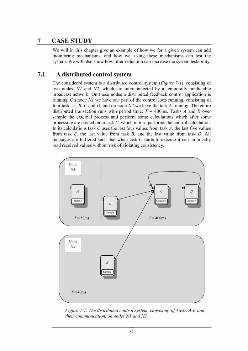
87

7 CASE STUDYWe will in this chapter give an example of how we for a given system can addmonitoring mechanisms, and how we, using these mechanisms can test thesystem. We will also show how jitter reduction can increase the system testability.

7.1 A distributed control systemThe considered system is a distributed control system (Figure 7-1), consisting oftwo nodes, N1 and N2, which are interconnected by a temporally predictablebroadcast network. On these nodes a distributed feedback control application isrunning. On node N1 we have one part of the control loop running, consisting offour tasks A, B, C and D, and on node N2 we have the task E running. The entiredistributed transaction runs with period time, T = 400ms. Tasks A and E oversample the external process and perform some calculations which after someprocessing are passed on to task C, which in turn performs the control calculation.In its calculations task C uses the last four values from task A, the last five valuesfrom task E, the last value from task B, and the last value from task D. Allmessages are buffered such that when task C starts to execute it can atomicallyread received values without risk of violating consistency.

A

Sample

C

Calculate

D

Actuate

T = 50ms T = 400ms

E

Sample

NodeN2

NodeN1

Figure 7-1. The distributed control system, consisting of Tasks A-E andtheir communication, on nodes N1 and N2.

B

Sample

T = 40ms

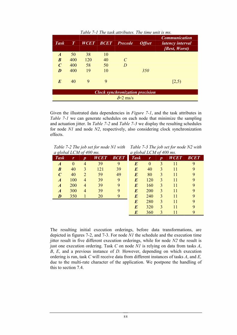
88

Given the illustrated data dependencies in Figure 7-1, and the task attributes inTable 7-1 we can generate schedules on each node that minimize the samplingand actuation jitter. In Table 7-2 and Table 7-3 we display the resulting schedulesfor node N1 and node N2, respectively, also considering clock synchronizationeffects.

The resulting initial execution orderings, before data transformations, aredepicted in figures 7-2, and 7-3. For node N1 the schedule and the execution timejitter result in five different execution orderings, while for node N2 the result isjust one execution ordering. Task C on node N1 is relying on data from tasks A,B, E, and a previous instance of D. However, depending on which executionordering is run, task C will receive data from different instances of tasks A, and E,due to the multi-rate character of the application. We postpone the handling ofthis to section 7.4.

Table 7-1 The task attributes. The time unit is ms.

Task T WCET BCET Precede OffsetCommunicationlatency interval

[Best, Worst)A 50 38 10B 400 120 40 CC 400 58 50 DD 400 19 10 350

E 40 9 9 [2,5)

Clock synchronization precisionδ=2 ms/s

Table 7-2 The job set for node N1 witha global LCM of 400 ms.Task r p WCET BCET

A 0 4 39 9B 40 3 121 39C 40 2 59 49A 100 4 39 9A 200 4 39 9A 300 4 39 9D 350 1 20 9

Table 7-3 The job set for node N2 witha global LCM of 400 ms.Task r p WCET BCET

E 0 3 11 9E 40 3 11 9E 80 3 11 9E 120 3 11 9E 160 3 11 9E 200 3 11 9E 240 3 11 9E 280 3 11 9E 320 3 11 9E 360 3 11 9

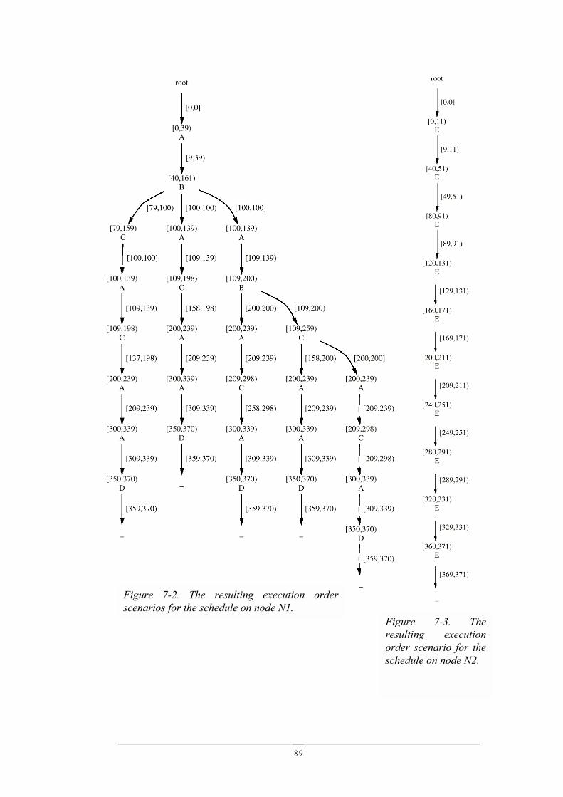
89

Figure 7-3. Theresulting executionorder scenario for theschedule on node N2.

Figure 7-2. The resulting execution orderscenarios for the schedule on node N1.

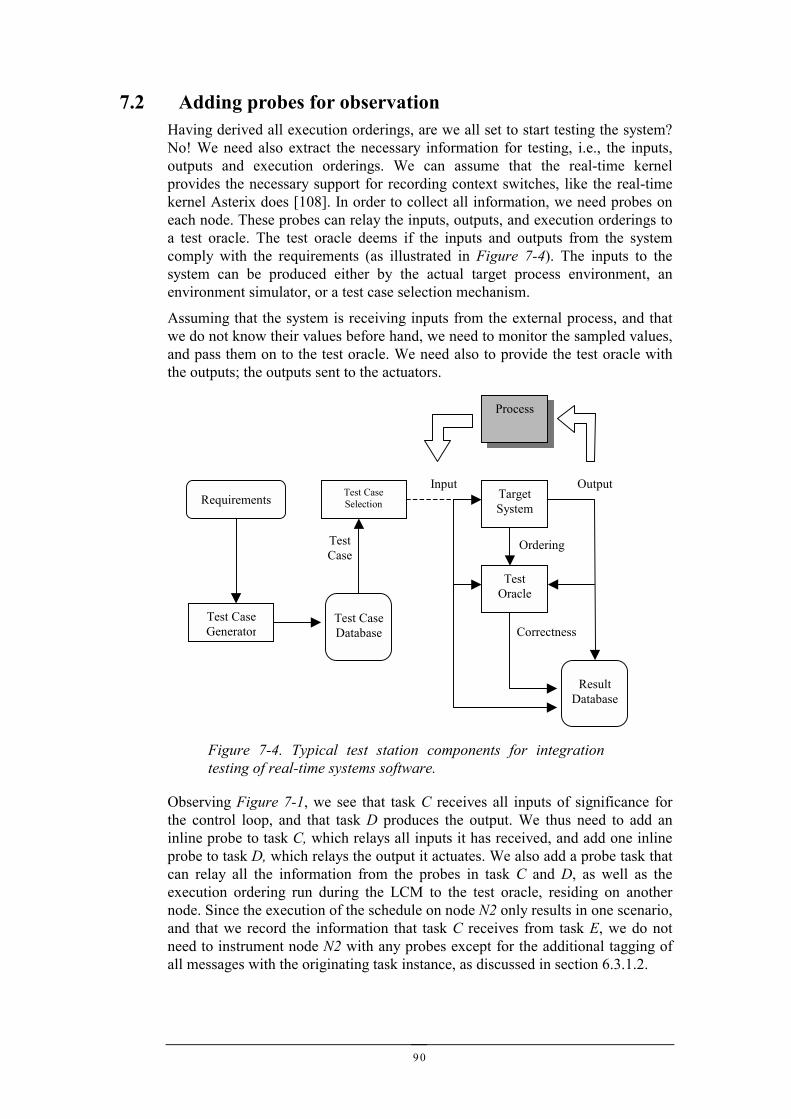
90

7.2 Adding probes for observationHaving derived all execution orderings, are we all set to start testing the system?No! We need also extract the necessary information for testing, i.e., the inputs,outputs and execution orderings. We can assume that the real-time kernelprovides the necessary support for recording context switches, like the real-timekernel Asterix does [108]. In order to collect all information, we need probes oneach node. These probes can relay the inputs, outputs, and execution orderings toa test oracle. The test oracle deems if the inputs and outputs from the systemcomply with the requirements (as illustrated in Figure 7-4). The inputs to thesystem can be produced either by the actual target process environment, anenvironment simulator, or a test case selection mechanism.

Assuming that the system is receiving inputs from the external process, and thatwe do not know their values before hand, we need to monitor the sampled values,and pass them on to the test oracle. We need also to provide the test oracle withthe outputs; the outputs sent to the actuators.

Observing Figure 7-1, we see that task C receives all inputs of significance forthe control loop, and that task D produces the output. We thus need to add aninline probe to task C, which relays all inputs it has received, and add one inlineprobe to task D, which relays the output it actuates. We also add a probe task thatcan relay all the information from the probes in task C and D, as well as theexecution ordering run during the LCM to the test oracle, residing on anothernode. Since the execution of the schedule on node N2 only results in one scenario,and that we record the information that task C receives from task E, we do notneed to instrument node N2 with any probes except for the additional tagging ofall messages with the originating task instance, as discussed in section 6.3.1.2.

TargetSystem

TestOracle

ResultDatabase

Test CaseSelection

Test CaseGenerator

Test CaseDatabase

RequirementsInput Output

Correctness

TestCase

Process

Ordering

Figure 7-4. Typical test station components for integrationtesting of real-time systems software.

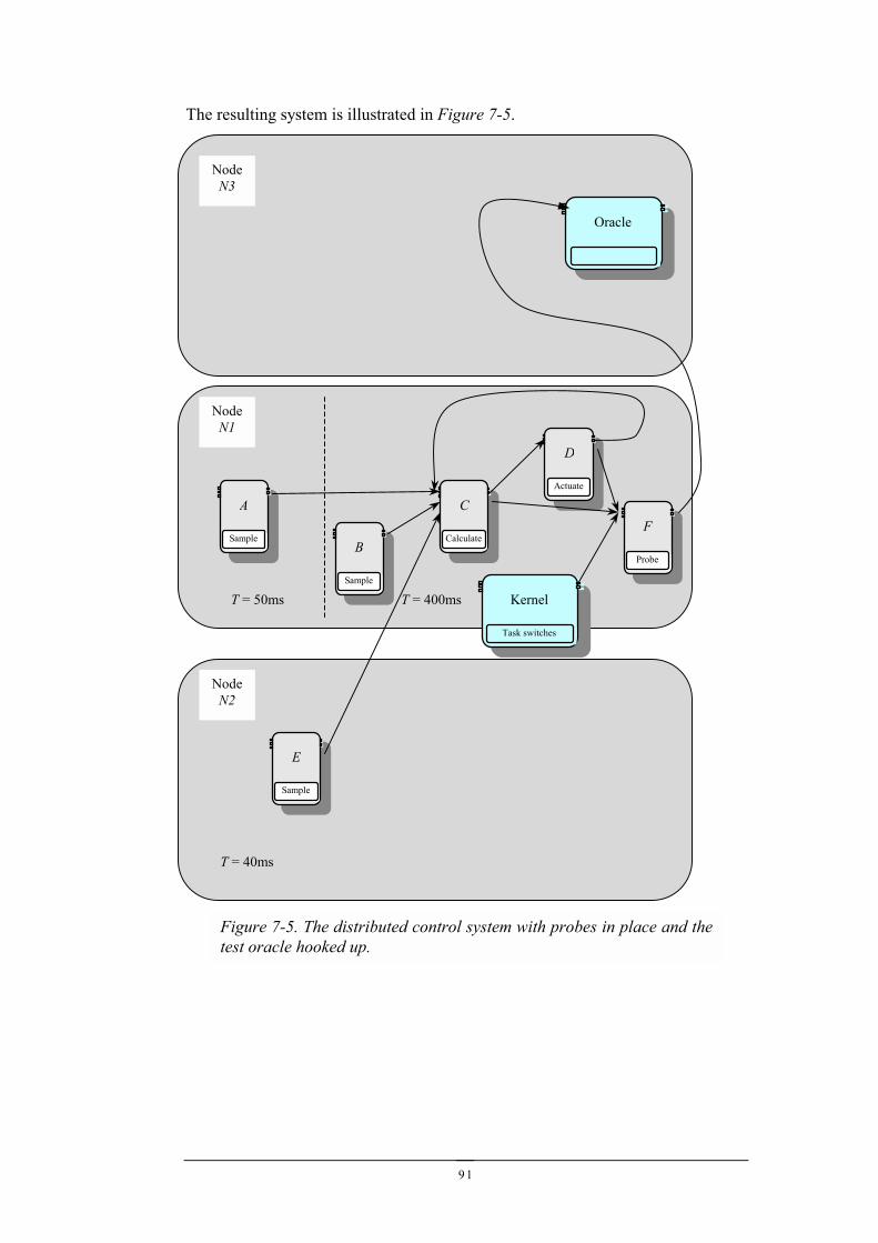
91

The resulting system is illustrated in Figure 7-5.

A

Sample

C

Calculate

D

Actuate

T = 50ms T = 400ms

E

Sample

NodeN2

NodeN1

B

Sample

T = 40ms

F

Probe

Kernel

Task switches

NodeN3

Oracle

Figure 7-5. The distributed control system with probes in place and thetest oracle hooked up.

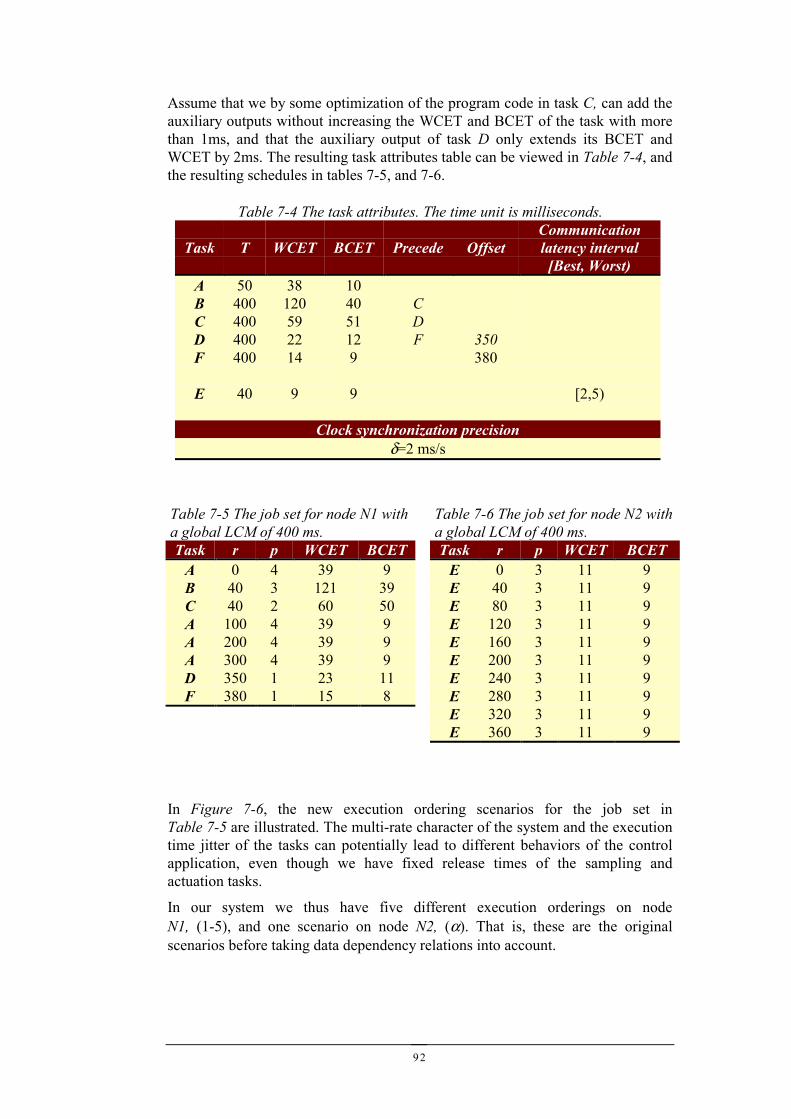
92

Assume that we by some optimization of the program code in task C, can add theauxiliary outputs without increasing the WCET and BCET of the task with morethan 1ms, and that the auxiliary output of task D only extends its BCET andWCET by 2ms. The resulting task attributes table can be viewed in Table 7-4, andthe resulting schedules in tables 7-5, and 7-6.

In Figure 7-6, the new execution ordering scenarios for the job set inTable 7-5 are illustrated. The multi-rate character of the system and the executiontime jitter of the tasks can potentially lead to different behaviors of the controlapplication, even though we have fixed release times of the sampling andactuation tasks.

In our system we thus have five different execution orderings on nodeN1, (1-5), and one scenario on node N2, (α). That is, these are the originalscenarios before taking data dependency relations into account.

Table 7-5 The job set for node N1 witha global LCM of 400 ms.Task r p WCET BCET

A 0 4 39 9B 40 3 121 39C 40 2 60 50A 100 4 39 9A 200 4 39 9A 300 4 39 9D 350 1 23 11F 380 1 15 8

Table 7-6 The job set for node N2 witha global LCM of 400 ms.Task r p WCET BCET

E 0 3 11 9E 40 3 11 9E 80 3 11 9E 120 3 11 9E 160 3 11 9E 200 3 11 9E 240 3 11 9E 280 3 11 9E 320 3 11 9E 360 3 11 9

Table 7-4 The task attributes. The time unit is milliseconds.

Task T WCET BCET Precede OffsetCommunicationlatency interval

[Best, Worst)A 50 38 10B 400 120 40 CC 400 59 51 DD 400 22 12 F 350F 400 14 9 380

E 40 9 9 [2,5)

Clock synchronization precisionδ=2 ms/s

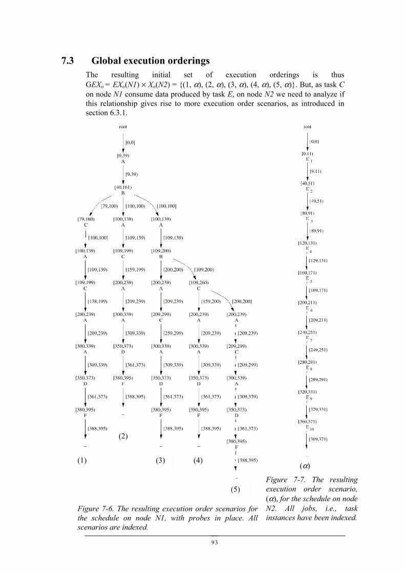
93

7.3 Global execution orderingsThe resulting initial set of execution orderings is thusGEXo = EXo(N1) × Xo(N2) = {(1, α), (2, α), (3, α), (4, α), (5, α)}. But, as task Con node N1 consume data produced by task E, on node N2 we need to analyze ifthis relationship gives rise to more execution order scenarios, as introduced insection 6.3.1.

(5)

Figure 7-6. The resulting execution order scenarios forthe schedule on node N1, with probes in place. Allscenarios are indexed.

(1)

(2)

(3) (4)(α)

Figure 7-7. The resultingexecution order scenario,(α), for the schedule on nodeN2. All jobs, i.e., taskinstances have been indexed.

2

3

4

5

6

8

9

10

1

7

94

7.4 Global execution ordering data dependency transformationBeginning with scenario (1, α) we see that task C has a start time interval ofstart(C) = [79,100). Considering the communication latency, [2,5), the onlycandidates are E2 and E3, thus scenario (1, α) transforms into scenario(1:E2, α), and (1:E3, α). Likewise:

• Scenario (2, α), where start(C) = [109,139), transforms into scenario(2:E3, α), and (2:E4, α).

• Scenario (3, α), where start(C) = [209,239), transforms into scenario(3:E5 α), and (3:E6, α).

• Scenario (4, α), where start(C) = [109,150), transforms into scenario(4:E3 α), and (4:E4, α).

• Scenario (5, α), where start(C) = [140,200), transforms into scenario(5:E4 α), and (5:E5, α).

The resulting global execution orderings set, GEXo, thus becomes:{(1:E2, α), (1:E3, α), (2:E3, α), (2:E4, α), (3:E5, α), (3:E6, α), (4:E3, α),(4:E4, α), (5:E4, α), (5:E5, α)}. Which we henceforth rename (1, α) … (10, α).

7.5 TestingAssuming that all sampling tasks sample the external process with 8bit A/Dconverters and that the actuator controls the process with an 8bit D/A converter,we get (28)4 = 232 input combinations, considering the feedback loop. This is ahuge state space, and we will thus never in practice be able to do exhaustivetesting, since running each LCM takes 400ms. Exhaustive testing would requirecontinuous testing for at least 54 years. One possibility is to resort to statisticalblack box testing, and decide on a reasonable level of reliability, and confidencein this reliability. As the tasks in the feedback control loop all work on the samephysical process it is however very likely that the sampled values by the tasks aredependent, which in practice will reduce the state space. Nonetheless, in this casestudy we assume that all input combinations are possible. Since we, as testers,cannot control the external process we have to settle for input observations. Thismeans that the basic assumption for statistical testing [6], that all inputs areunique, do not hold. Consequently, we can run the same test case over and overagain. The test oracle does thus need to remember if the same test case has beenrun or not. Having assumed all this we can start testing the system. The teststation can be viewed in Figure 7-8. Table 7-7 lists the resulting number of testcases and the time required for testing one scenario and ten scenariosrespectively.

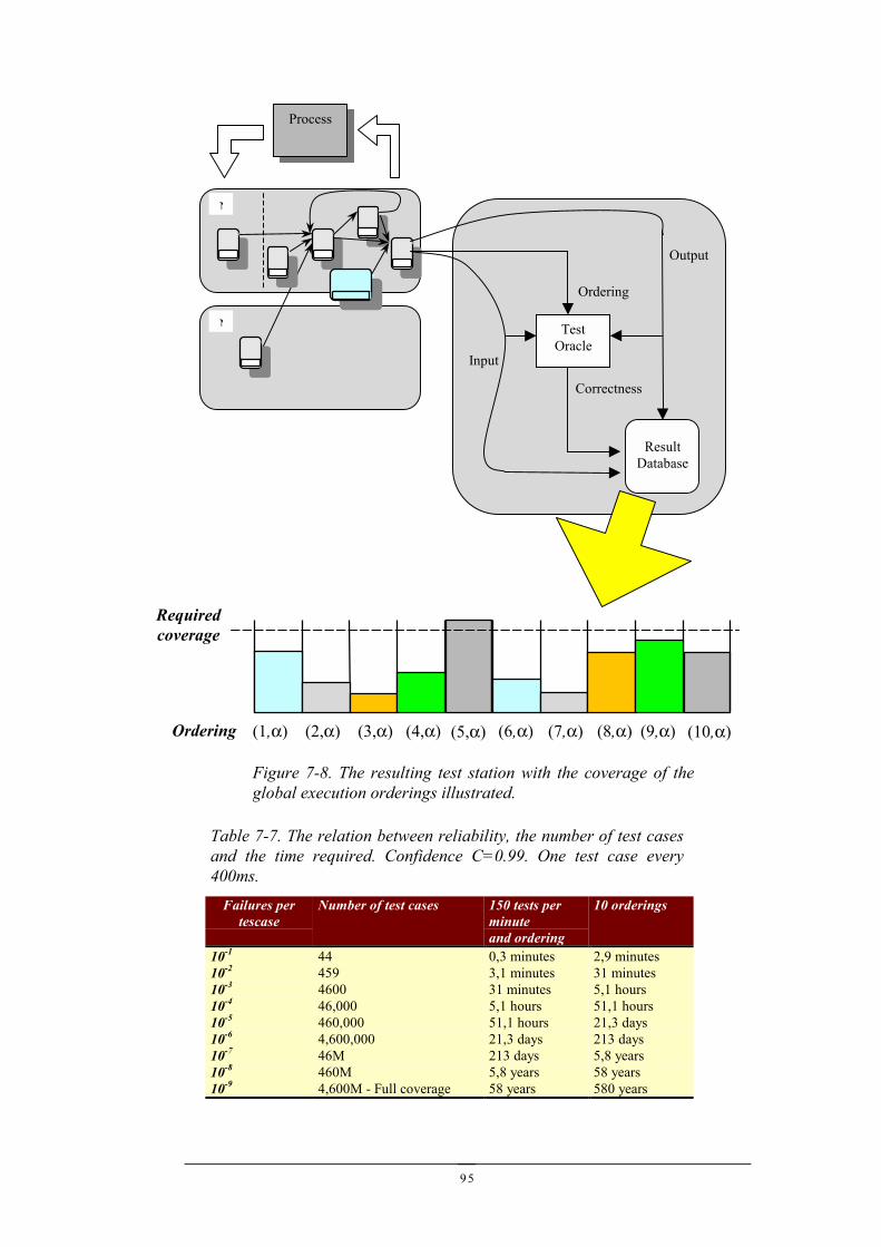
95

TestOracle

ResultDatabase

Input

Output

Correctness

Process

Ordering

N

N

Requiredcoverage

Ordering

Figure 7-8. The resulting test station with the coverage of theglobal execution orderings illustrated.

(6,α) (7,α) (9,α)(8,α) (10,α)(1,α) (2,α) (4,α)(3,α) (5,α)

Table 7-7. The relation between reliability, the number of test casesand the time required. Confidence C=0.99. One test case every400ms.

Failures pertescase

Number of test cases 150 tests perminuteand ordering

10 orderings

10-1 44 0,3 minutes 2,9 minutes10-2 459 3,1 minutes 31 minutes10-3 4600 31 minutes 5,1 hours10-4 46,000 5,1 hours 51,1 hours10-5 460,000 51,1 hours 21,3 days10-6 4,600,000 21,3 days 213 days10-7 46M 213 days 5,8 years10-8 460M 5,8 years 58 years10-9 4,600M - Full coverage 58 years 580 years

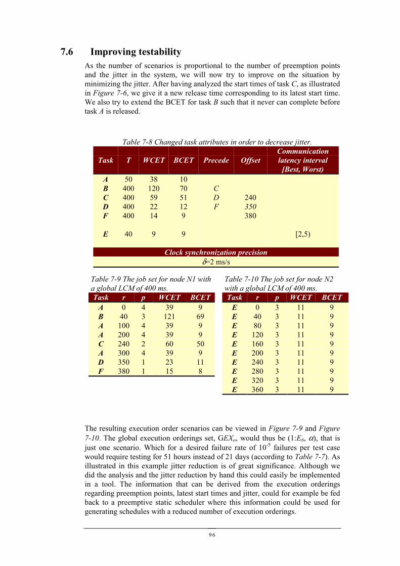
96

7.6 Improving testabilityAs the number of scenarios is proportional to the number of preemption pointsand the jitter in the system, we will now try to improve on the situation byminimizing the jitter. After having analyzed the start times of task C, as illustratedin Figure 7-6, we give it a new release time corresponding to its latest start time.We also try to extend the BCET for task B such that it never can complete beforetask A is released.

The resulting execution order scenarios can be viewed in Figure 7-9 and Figure7-10. The global execution orderings set, GEXo, would thus be (1:E6, α), that isjust one scenario. Which for a desired failure rate of 10-5 failures per test casewould require testing for 51 hours instead of 21 days (according to Table 7-7). Asillustrated in this example jitter reduction is of great significance. Although wedid the analysis and the jitter reduction by hand this could easily be implementedin a tool. The information that can be derived from the execution orderingsregarding preemption points, latest start times and jitter, could for example be fedback to a preemptive static scheduler where this information could be used forgenerating schedules with a reduced number of execution orderings.

Table 7-9 The job set for node N1 witha global LCM of 400 ms.Task r p WCET BCET

A 0 4 39 9B 40 3 121 69A 100 4 39 9A 200 4 39 9C 240 2 60 50A 300 4 39 9D 350 1 23 11F 380 1 15 8

Table 7-10 The job set for node N2with a global LCM of 400 ms.Task r p WCET BCET

E 0 3 11 9E 40 3 11 9E 80 3 11 9E 120 3 11 9E 160 3 11 9E 200 3 11 9E 240 3 11 9E 280 3 11 9E 320 3 11 9E 360 3 11 9

Table 7-8 Changed task attributes in order to decrease jitter.

Task T WCET BCET Precede OffsetCommunicationlatency interval[Best, Worst)

A 50 38 10B 400 120 70 CC 400 59 51 D 240D 400 22 12 F 350F 400 14 9 380

E 40 9 9 [2,5)

Clock synchronization precisionδ=2 ms/s

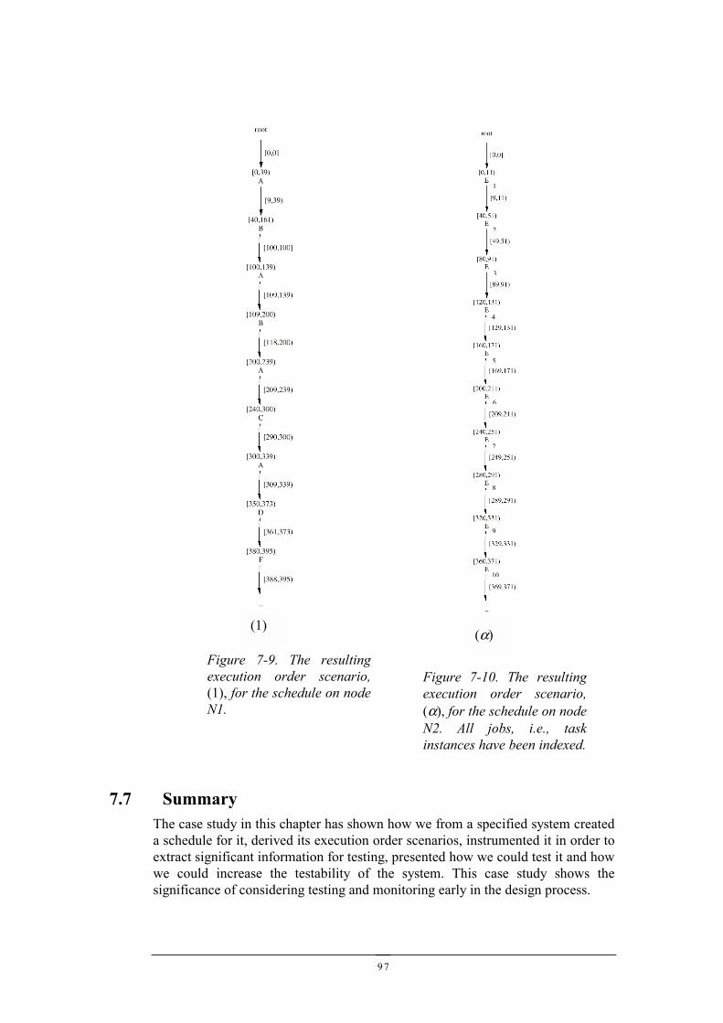
97

7.7 SummaryThe case study in this chapter has shown how we from a specified system createda schedule for it, derived its execution order scenarios, instrumented it in order toextract significant information for testing, presented how we could test it and howwe could increase the testability of the system. This case study shows thesignificance of considering testing and monitoring early in the design process.

Figure 7-10. The resultingexecution order scenario,(α), for the schedule on nodeN2. All jobs, i.e., taskinstances have been indexed.

(α)

2

3

4

5

6

8

9

10

1

7

Figure 7-9. The resultingexecution order scenario,(1), for the schedule on nodeN1.

(1)

98

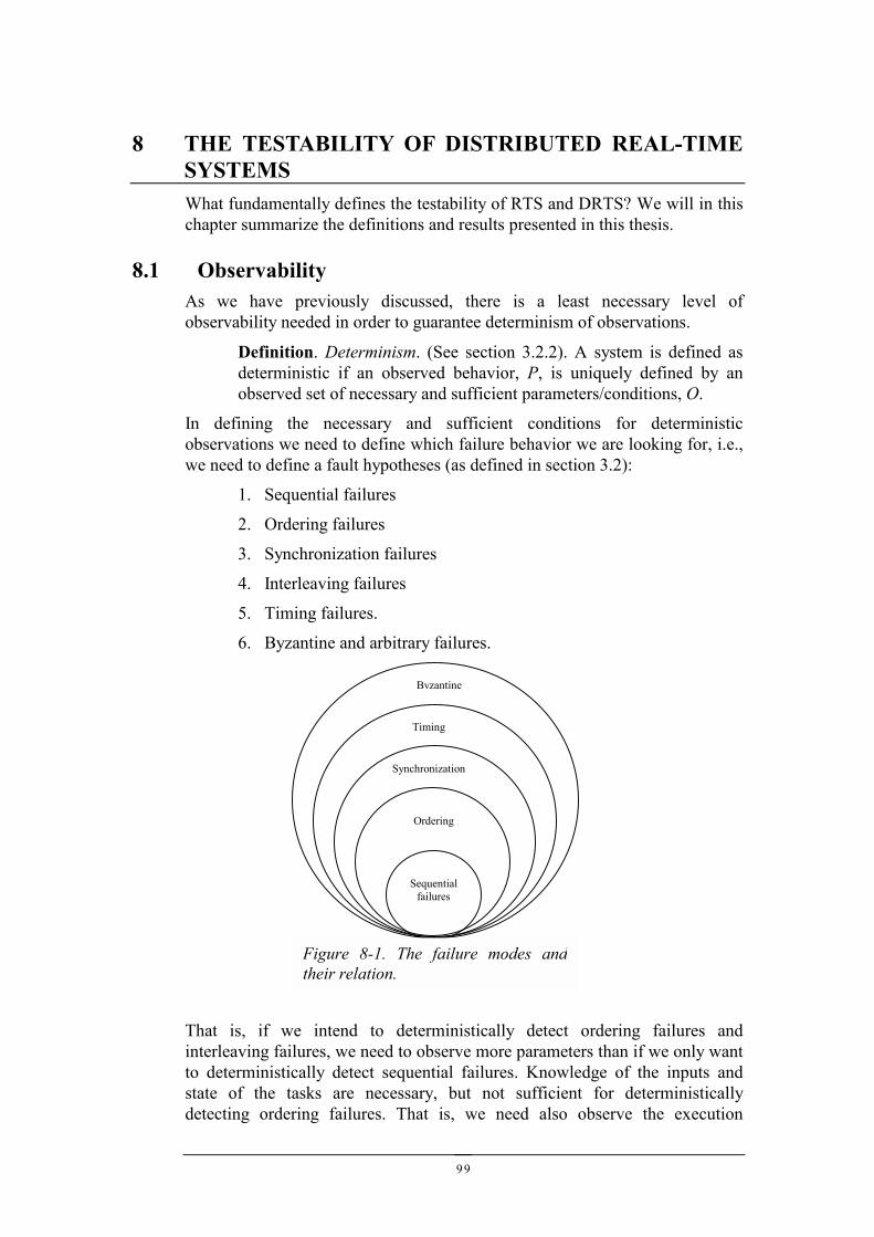
99

8 THE TESTABILITY OF DISTRIBUTED REAL-TIMESYSTEMSWhat fundamentally defines the testability of RTS and DRTS? We will in thischapter summarize the definitions and results presented in this thesis.

8.1 ObservabilityAs we have previously discussed, there is a least necessary level ofobservability needed in order to guarantee determinism of observations.

Definition. Determinism. (See section 3.2.2). A system is defined asdeterministic if an observed behavior, P, is uniquely defined by anobserved set of necessary and sufficient parameters/conditions, O.

In defining the necessary and sufficient conditions for deterministicobservations we need to define which failure behavior we are looking for, i.e.,we need to define a fault hypotheses (as defined in section 3.2):

1. Sequential failures

2. Ordering failures

3. Synchronization failures

4. Interleaving failures

5. Timing failures.

6. Byzantine and arbitrary failures.

That is, if we intend to deterministically detect ordering failures andinterleaving failures, we need to observe more parameters than if we only wantto deterministically detect sequential failures. Knowledge of the inputs andstate of the tasks are necessary, but not sufficient for deterministicallydetecting ordering failures. That is, we need also observe the execution

Byzantine

Timing

Synchronization

Ordering

Sequentialfailures

Figure 8-1. The failure modes andtheir relation.

100

orderings of the tasks. Likewise for deterministic observations of interleavingfailures, e.g., non-reentrant code, we need, in addition, to observe the orderingof task interleavings, also observe the exact timing (down to the exact machinecode instruction) when task interleavings occur, as done in the deterministicreplay in chapter 5. In contrast, if we are just looking for failures pertaining tosequential failure modes, it would be overkill to observe the system to such alevel that we can deterministically observe interleaving failures.

However, if the fault hypothesis is interleaving failures, but we have aninfrastructure that supports memory protection, we would be able to reducesome, if not all, interleaving failures pertaining to memory corruption and non-reentrant code. We would then be able to reduce the fault hypothesis tosynchronization, or even orderings failures, and therefore reduce theinformation necessary for observations. If we then, with memory protectionsupport, observe, test, and debug the system, we can achieve a certain level ofreliability. However, if we later remove the memory protection, more severefailure modes can occur, and we can thus not guarantee the achievedreliability, and as we have reduced the level of observation we cannotguarantee that the observations are deterministic. We will elaborate on this inthe future work in chapter 9.

8.2 CoverageIn order to establish a certain level of confidence in the correctness of asystem, we need to define coverage criteria, i.e., criteria on how much testingis required. This is typically defined in terms of sets of possible system statesthat must be explored. Examples are fractions of possible inputs tested,fractions of program paths tested, or in our case the number of executionorderings that needs to be explored. Consequently is the testability of aprogram a function of the number of states we must explore.

8.3 ControllabilityIn order to track down errors, achieve sufficient coverage when testing, or tofacilitate regression testing, we need to reproduce observations and failures.

Definition. Reproducibility. (See section 3.2). A system is reproducibleif it is deterministic with respect to a behavior P, and it is possible tocontrol the entire set of necessary and sufficient conditions, O.

Definition. Partial reproducibility. (See section 3.2). A system ispartially reproducible if it is deterministic with respect to a behavior P,and it is possible to control a subset of the necessary and sufficientconditions, O.

101

8.4 TestabilityBased on the above we can conclude that that the testability of a real-timesystem is a function of:

• the fault hypothesis

• the extent to which the necessary and sufficient parameters for thatfault hypotheses can be observed,

• the ability to control these parameters, and

• coverage.

The testability of a system pertaining to this definition is thus dependent on theinfrastructure available, i.e., to which extent we can observe the system, whichfault hypothesis we can discard, and on the number of behaviors we need toconsider (coverage). The latter is facilitated by the infrastructure’s support forcontrol over all parameters necessary for achieving sufficient coverage.

102

103

9 CONCLUSIONSWe have in this thesis shown that dynamic verification by testing can never beeliminated when developing reliable software. Even if we make use of formalmethods or fault tolerance techniques we will never be able to do away withtesting, since testing can be used to validate underlying assumptions and thefidelity of models. Software reliability is essential in computer controlled safety-critical systems, all of which (with a few exceptions) are real-time systems, andfrequently also distributed real-time systems. Any testing of safety-criticalsystems has thus to take into account the peculiarities of real-time systems (RTS)and of distributed real-time systems (DRTS).

We have in this paper described, discussed and provide solutions to a number ofareas:

Monitoring

We have presented a framework for monitoring single tasking, multi-tasking, anddistributed real-time systems. This includes a description of what to observe, howto eliminate the disturbances caused by the actual act of observing (the probeeffect), how to correlate observations between nodes (how to define a globalstate), and how to reproduce the observations. We have given a taxonomy ofdifferent observation techniques, and identified where, how and when thesetechniques should be applied for deterministic observations. We have argued thatit is essential to consider monitoring early in the design process, in order toachieve efficient and deterministic observations.

Debugging

We have presented a method for deterministic debugging of distributed real-timesystems, which to our knowledge is

• The first entirely software based method for deterministic debugging of singletasking and multi-tasking real-time systems.

• The first method for deterministic debugging of distributed real-time systems.

The method relies on an instrumented kernel to on-line record the occurrencesand timings of major system events. The recording can then, using a specialdebug kernel, be replayed off-line to faithfully reproduce the functional andtemporal behavior of the recorded execution, while allowing standard debuggingusing break points etc. to be applied.

The method scales from debugging of single real-time tasks, to multi-tasking anddistributed multitasking systems.

The cost for this dramatically increased debugging capability is the overheadinduced by the kernel instrumentation and by instrumentation of the applicationcode. To eliminate probe-effects, these instrumentations should remain in thedeployed system. We are however convinced that this is a justifiable penalty formany applications.

104

Testing

We have in this thesis introduced a novel method for deterministic testing ofmultitasking and distributed real-time systems. We have specifically addressedtask sets with recurring release patterns, executing in a distributed system with aglobally synchronized time base, and where the scheduling on each node ishandled by a priority driven preemptive scheduler. The results can be summed upto:

• We have provided a technique for finding all the possible execution scenariosfor a DRTS with preemption and jitter.

• We have proposed a testing strategy for deterministic and reproducible testingof DRTS.

• A benefit of the testing strategy is that it allows any testing technique forsequential software to be used to test DRTS.

• Jitter increases the number of execution order scenarios, and jitter reductiontechniques should therefore be used whenever possible to increase testability.

• The number of execution orderings is an objective measure of the testabilityof DRTS, which can be used as a new scheduling optimization criterion forgenerating schedules that are easier to test, or simply make it possible tocompare different designs with respect to testability.

• We can use the execution order analysis for calculating the exact best-caseand worst-case response-times for jobs, as well as calculating response-timejitter of the jobs. We could thus make use of the execution order analysis forschedulability analysis of strictly periodic fixed priority scheduled systemswith offsets.

Testability

We have in this thesis also argued that testability is an essential property of asystem, and that it is necessary to try to maximize the testability. The problems ofdesigning and verifying software are fundamental in character: software has adiscontinuous behavior, no inertia, and has no physical restrictions what so ever,except for time. Thus, we cannot make use of interpolation or extrapolation whentesting, and we conclude that it is essential to design for high testability. Ifsoftware engineering is going to be established as a real engineering discipline wemust take the quest for high testability seriously.

Finally

Any programming language, any formal method, any theory of scheduling, anyfault tolerance technique and any testing technique will always be flawed orincomplete. To design reliable software we must thus make use of all theseconcepts in union. Consequently we will never be able to eliminate testingcompletely. However, with respect to testing, debugging and monitoring of real-time systems software there has been very little work done. Relating to what waswritten in the introduction of this thesis, we believe however that thecontributions of this thesis increase the depth on the shallow side of the DRTSverification pool of knowledge (no risk of drowning though).

105

10 FUTURE WORKIn this chapter we will outline some issues that we consider relevant and important topursue in the future. We will begin with some extensions to the work presented inthis thesis, and then widen the scope by discussing the use of components in real-time systems, i.e., reusable software entities, and how these components affect thepotential reliability, and verification required.

10.1 Monitoring, testing and debuggingWith respect to the results presented in this thesis we suggest the followingextensions and pursuits:

• Experimentally validate the usefulness of the presented results. This pursuitwill hopefully be facilitated by the use of the real-time kernel Asterix [108]that has specifically been developed to give the necessary support formonitoring, debugging and testing.

• Extend the execution ordering analysis to also encompass critical regions, byfor example assuming immediate inheritance protocols for resource sharing.This analysis would however necessitate assumptions about the duration ofthe critical regions (intervals), and assumptions about the intervals of delaybefore entering the critical regions. Knowing these parameters we believe itis straightforward to extend the execution ordering analysis.

• Devise an exact analysis (less pessimistic) for interrupt interference on theexecution order graph. The method presented in this thesis is ratherpessimistic when the duration between releases of tasks is non-harmoniouswith the inter-arrival times of the interrupts. It is safe but pessimistic. Forexample, consider a system where we have two tasks, A and B, where task Bhas the highest priority, where rA=0, WCETA = 3, rB = 4, WCETB = 3, and aninterrupt with a Tmin = 3, and a service routine with a WCET of 1. Theresponse time for both tasks, just considering their execution time and theworst case interference by the interrupt, is 5 (two interrupt hits each). It ishowever not possible for both tasks to be hit twice by the interrupt during thesame scenario. We therefore suggest an extension of the analysis to minimizethe pessimism by taking these types of situations into account.

• Complete coverage for the distributed system would naively be allcombinations of all local execution order scenarios (as introduced in section6.3.1). Depending on the design, many of the combinations would howeverbe infeasible due to data dependencies, with the consequence that a certainscenario on one node always gives a specific scenario on another node.Reductions that take these factors into account should be further investigated.One possibility to reduce the required coverage could be to performparallel composition of the individual EOGs, using standard techniquesfor composing timed transition systems [101], this would probably reducethe pessimism introduced in the GEXo data dependency transformation.

We will now continue with a discussion on software reuse in real-time systems andwhat the effects are on verification.

106

10.2 Formal and probabilistic arguments for component reuseand testing in safety-critical real-time systems

In this section we will discuss how testing of real-time software relates tocomponent reuse in safety-critical real-time systems. Reuse of softwarecomponents is a new alleged silver bullet that will kill all bugs. This, as for allpreviously alleged silver bullets is of course just a myth. Experience of softwarereuse has shown that re-verification cannot be eliminated in general, which forsafety-critical systems is a significant problem since verification is the singlemost cost and time consuming activity during system development (as discussedin chapter 2).

In order to remedy this situation we will introduce a novel framework for formaland probabilistic arguments of component reuse and re-verification in safety-critical real-time systems. Using both quantitative and qualitative descriptions ofcomponent attributes and assumptions about the environment, we can relateinput-output domains, temporal characteristics, fault hypotheses, reliability levels,and task models. Using these quantitative and qualitative attributes we can deemif a component can be reused without re-verification or not. We can also deemhow much and which subsets, of say input-output domains, that need additionalfunctional testing.

In order to be able to design software that is as safe and reliable as the mechanicalor electromechanical parts it replaces, and to reduce the time to market, focus ofcurrent research and practice has turned to the reuse of proven softwarecomponents. The basic idea is that the system designer should be able to procure(or reuse) software components in the same manner as hardware components canbe acquired. Hardware components like nuts, bolts, CPUs, memory, A/Dconverters can be procured based on functionality, running conditions (theenvironment) and their reliability. Hardware components are typically dividedinto two classes, commercial and military grade components, where militarygrade electronics can withstand greater temperature spans, handle shock andhumidity better than commercial components. However, for software it is not soeasy to make the same classification since the metrics of software are not basedon physical attributes, but rather on its design, which is unique for each newdesign. As mentioned in the background of this thesis, software has no physicalrestrictions what so ever and the sole physical entity that can be modeled andmeasured by software engineers is time.

We will in this section elaborate on this idea of components for safety-criticalreal-time systems. The arguments for reuse of software (components) are usuallyarguments for rapid prototyping (reusing code), arguments for outsourcing, andarguments for higher reliability. In the latter case it is assumed that verification ofthe components can be eliminated and that the reliability of the component can be“inherited” from previous uses. Expensive and catastrophic experiences havehowever shown that it is not so simple: Ariane 5, and Therac 25. The explosion ofthe Ariane rocket [43][62], and the accidents due to excessive dosage by theradiotherapy machine Therac 25 [66] were all due to misconceptions, ordisregard, of changes in the target environment from earlier uses of the software(Ariane 4 and Therac 20). The believed proven reliability of the components hadno bearing in the new environments where they were reused. The belief in thereliability of the components meant in the cases of Ariane5 and Therac 25 that re-

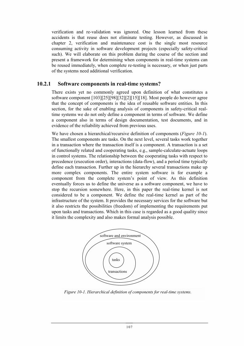
107

verification and re-validation was ignored. One lesson learned from theseaccidents is that reuse does not eliminate testing. However, as discussed inchapter 2, verification and maintenance cost is the single most resourceconsuming activity in software development projects (especially safety-criticalsuch). We will elaborate on this problem during the course of the section andpresent a framework for determining when components in real-time systems canbe reused immediately, when complete re-testing is necessary, or when just partsof the systems need additional verification.

10.2.1 Software components in real-time systems?There exists yet no commonly agreed upon definition of what constitutes asoftware component [103][25][98][32][2][15][18]. Most people do however agreethat the concept of components is the idea of reusable software entities. In thissection, for the sake of enabling analysis of components in safety-critical real-time systems we do not only define a component in terms of software. We definea component also in terms of design documentation, test documents, and inevidence of the reliability achieved from previous uses.

We have chosen a hierarchical/recursive definition of components (Figure 10-1).The smallest components are tasks. On the next level, several tasks work togetherin a transaction where the transaction itself is a component. A transaction is a setof functionally related and cooperating tasks, e.g., sample-calculate-actuate loopsin control systems. The relationship between the cooperating tasks with respect toprecedence (execution order), interactions (data-flow), and a period time typicallydefine each transaction. Further up in the hierarchy several transactions make upmore complex components. The entire system software is for example acomponent from the complete system’s point of view. As this definitioneventually forces us to define the universe as a software component, we have tostop the recursion somewhere. Here, in this paper the real-time kernel is notconsidered to be a component. We define the real-time kernel as part of theinfrastructure of the system. It provides the necessary services for the software butit also restricts the possibilities (freedom) of implementing the requirements putupon tasks and transactions. Which in this case is regarded as a good quality sinceit limits the complexity and also makes formal analysis possible.

Figure 10-1. Hierarchical definition of components for real-time systems.

tasks

transactions

software system

software and environment

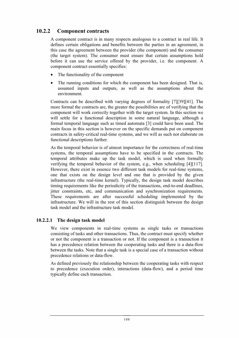
108

10.2.2 Component contractsA component contract is in many respects analogous to a contract in real life. Itdefines certain obligations and benefits between the parties in an agreement, inthis case the agreement between the provider (the component) and the consumer(the target system). The consumer must ensure that certain assumptions holdbefore it can use the service offered by the provider, i.e. the component. Acomponent contract essentially specifies:

• The functionality of the component

• The running conditions for which the component has been designed. That is,assumed inputs and outputs, as well as the assumptions about theenvironment.

Contracts can be described with varying degrees of formality [7][39][41]. Themore formal the contracts are, the greater the possibilities are of verifying that thecomponent will work correctly together with the target system. In this section wewill settle for a functional description in some natural language, although aformal temporal language such as timed automata [3] could have been used. Themain focus in this section is however on the specific demands put on componentcontracts in safety-critical real-time systems, and we will as such not elaborate onfunctional descriptions further.

As the temporal behavior is of utmost importance for the correctness of real-timesystems, the temporal assumptions have to be specified in the contracts. Thetemporal attributes make up the task model, which is used when formallyverifying the temporal behavior of the system, e.g., when scheduling [4][117].However, there exist in essence two different task models for real-time systems,one that exists on the design level and one that is provided by the giveninfrastructure (the real-time kernel). Typically, the design task model describestiming requirements like the periodicity of the transactions, end-to-end deadlines,jitter constraints, etc, and communication and synchronization requirements.These requirements are after successful scheduling implemented by theinfrastructure. We will in the rest of this section distinguish between the designtask model and the infrastructure task model.

10.2.2.1 The design task modelWe view components in real-time systems as single tasks or transactionsconsisting of tasks and other transactions. Thus, the contract must specify whetheror not the component is a transaction or not. If the component is a transaction ithas a precedence relation between the cooperating tasks and there is a data-flowbetween the tasks. Note that a single task is a special case of a transaction withoutprecedence relations or data-flow.

As defined previously the relationship between the cooperating tasks with respectto precedence (execution order), interactions (data-flow), and a period timetypically define each transaction.

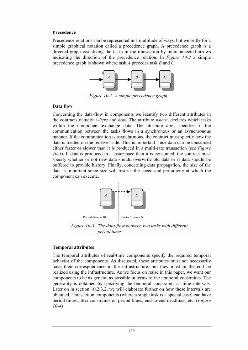
109

Precedence

Precedence relations can be represented in a multitude of ways, but we settle for asimple graphical notation called a precedence graph. A precedence graph is adirected graph visualizing the tasks in the transaction by interconnected arrowsindicating the direction of the precedence relation. In Figure 10-2 a simpleprecedence graph is shown where task A precedes task B and C.

Data flow

Concerning the data-flow in components we identify two different attributes inthe contracts namely: where and how. The attribute where, declares which taskswithin the component exchange data. The attribute how, specifies if thecommunication between the tasks flows in a synchronous or an asynchronousmanner. If the communication is asynchronous, the contract must specify how thedata is treated on the receiver side. This is important since data can be consumedeither faster or slower than it is produced in a multi-rate transaction (see Figure10-3). If data is produced in a faster pace than it is consumed, the contract mustspecify whether or not new data should overwrite old data or if data should bebuffered to provide history. Finally, concerning data propagation, the size of thedata is important since size will restrict the speed and periodicity at which thecomponent can execute.

Temporal attributes

The temporal attributes of real-time components specify the required temporalbehavior of the components. As discussed, these attributes must not necessarilyhave their correspondence in the infrastructure, but they must in the end berealized using the infrastructure. As we focus on reuse in this paper, we want ourcomponents to be as general as possible in terms of the temporal constraints. Thegenerality is obtained by specifying the temporal constraints as time intervals.Later on in section 10.2.3.2, we will elaborate further on how these intervals areobtained. Transaction components (where a single task is a special case) can haveperiod times, jitter constraints on period times, end-to-end deadlines, etc. (Figure10-4)

Figure 10-2. A simple precedence graph.

A B C

Figure 10-3. The data-flow between two tasks with differentperiod times.

Period time = 10 Period time = 5

A D

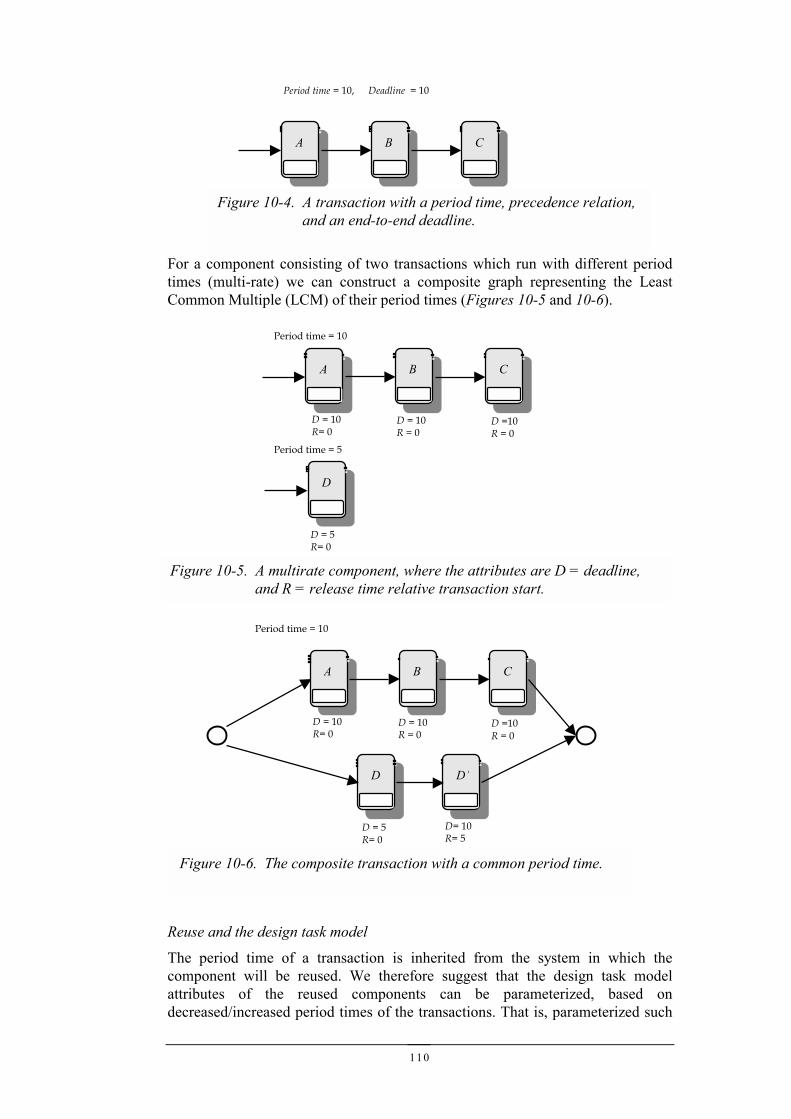
110

For a component consisting of two transactions which run with different periodtimes (multi-rate) we can construct a composite graph representing the LeastCommon Multiple (LCM) of their period times (Figures 10-5 and 10-6).

Reuse and the design task model

The period time of a transaction is inherited from the system in which thecomponent will be reused. We therefore suggest that the design task modelattributes of the reused components can be parameterized, based ondecreased/increased period times of the transactions. That is, parameterized such

Figure 10-4. A transaction with a period time, precedence relation,and an end-to-end deadline.

Period time = 10, Deadline = 10

A B C

A B C

Figure 10-5. A multirate component, where the attributes are D = deadline,and R = release time relative transaction start.

Period time = 10

D = 10R= 0

D = 10R = 0

D =10R = 0

Period time = 5

D = 5R= 0

D

D

Period time = 10

D = 10R= 0

D = 10R = 0

D =10R = 0

D = 5R= 0

D= 10R= 5

Figure 10-6. The composite transaction with a common period time.

A B C

D’

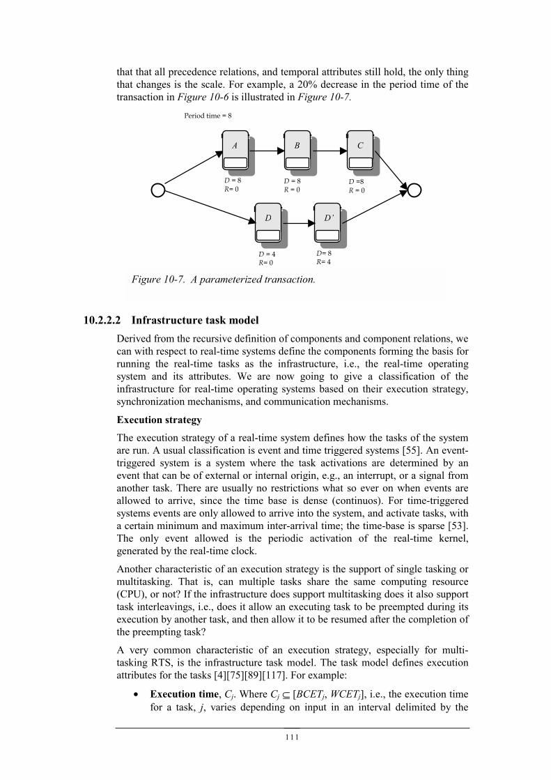
111

that that all precedence relations, and temporal attributes still hold, the only thingthat changes is the scale. For example, a 20% decrease in the period time of thetransaction in Figure 10-6 is illustrated in Figure 10-7.

10.2.2.2 Infrastructure task modelDerived from the recursive definition of components and component relations, wecan with respect to real-time systems define the components forming the basis forrunning the real-time tasks as the infrastructure, i.e., the real-time operatingsystem and its attributes. We are now going to give a classification of theinfrastructure for real-time operating systems based on their execution strategy,synchronization mechanisms, and communication mechanisms.

Execution strategy

The execution strategy of a real-time system defines how the tasks of the systemare run. A usual classification is event and time triggered systems [55]. An event-triggered system is a system where the task activations are determined by anevent that can be of external or internal origin, e.g., an interrupt, or a signal fromanother task. There are usually no restrictions what so ever on when events areallowed to arrive, since the time base is dense (continuos). For time-triggeredsystems events are only allowed to arrive into the system, and activate tasks, witha certain minimum and maximum inter-arrival time; the time-base is sparse [53].The only event allowed is the periodic activation of the real-time kernel,generated by the real-time clock.

Another characteristic of an execution strategy is the support of single tasking ormultitasking. That is, can multiple tasks share the same computing resource(CPU), or not? If the infrastructure does support multitasking does it also supporttask interleavings, i.e., does it allow an executing task to be preempted during itsexecution by another task, and then allow it to be resumed after the completion ofthe preempting task?

A very common characteristic of an execution strategy, especially for multi-tasking RTS, is the infrastructure task model. The task model defines executionattributes for the tasks [4][75][89][117]. For example:

• Execution time, Cj. Where Cj ⊆ [BCETj, WCETj], i.e., the execution timefor a task, j, varies depending on input in an interval delimited by the

D

Period time = 8

D = 8R= 0

D = 8R = 0

D =8R = 0

D = 4R= 0

D= 8R= 4

Figure 10-7. A parameterized transaction.

A B C

D’

112

task’s best case execution time (BCETj) and its worst case execution time(WCETj).

• Periodicity, Tj. Where Tj ⊆ [Tjmin, Tj

max], i.e., the inter-arrival timebetween the activations of a task, j, is delimited by an interval rangingfrom the minimum inter-arrival time, to the maximum inter-arrival time.For strictly periodic RTS, Tj

min = Tjmax.

• Release time, Rj. Where Rj defines an offset relative the period start atwhich the task j should be activated. Release time also go by the nameOffset.

• Priority, Pj. Where Pj defines the priority of task j. When several tasksare activated at the same time, or when an activated task has higherpriority than the currently running task, the priority determines which taskshould have access to the computing resource.

• Deadline, Dj. Where Dj defines the deadline for the task, j, that is, when ithas to be finished. The deadline can be defined relative task activation, itsperiod time, absolute time, etc.

For different infrastructures the task model vary with different flavors of theabove-exemplified attributes.

Synchronization

Depending on the infrastructure we can either make necessary synchronizationsbetween tasks off-line if it is time triggered and supports offsets, or we cansynchronize tasks on-line using primitives like semaphores. In the off-line casewe guarantee precedence and mutual exclusion relations by separating tasks time-wise, using offsets.

Communication

Communication between tasks in RTS can be achieved in a multitude of ways.We can make use of shared memory which is guarded by semaphores, or timesynchronization, or we can via the operating system infrastructure send messages,or signals between tasks. Depending on the relation between the communicatingtasks, in respect to periodicity, the communication can vary between totallysynchronous communication to totally asynchronous communication. That is, iftask i sends data to task j, and both tasks have equal periodicity, Tj = Ti, we canmake use of just one shared memory buffer. However, if Tj > Ti or Tj < Ti theissue gets more complicated. Either we make use of overwriting semantics (state-based communication), using just a few buffers, or we record all data that hasbeen sent by the higher frequency task so that it can be consumed by the lowerfrequency task when it is activated. There are several approaches to solving thisproblem [26][52][13].

10.2.3 Component contract analysisWe are now going to introduce a framework for formal and probabilisticarguments of component reuse in safety-critical real-time systems. The basic ideais to provide evidence, based on the components contracts and the experienceaccumulated, that a component can be reused immediately, or if only parts can bereused - or not at all. That is, we want to relate the environment for which thecomponent was originally designed and verified, with the new environment where

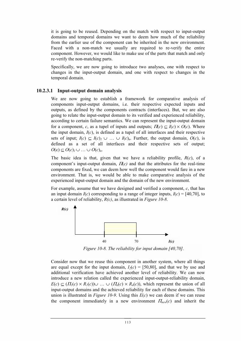
113

it is going to be reused. Depending on the match with respect to input-outputdomains and temporal domains we want to deem how much of the reliabilityfrom the earlier use of the component can be inherited in the new environment.Faced with a non-match we usually are required to re-verify the entirecomponent. However, we would like to make use of the parts that match and onlyre-verify the non-matching parts.

Specifically, we are now going to introduce two analyses, one with respect tochanges in the input-output domain, and one with respect to changes in thetemporal domain.

10.2.3.1 Input-output domain analysisWe are now going to establish a framework for comparative analysis ofcomponents input-output domains, i.e. their respective expected inputs andoutputs, as defined by the components contracts (interfaces). But, we are alsogoing to relate the input-output domain to its verified and experienced reliability,according to certain failure semantics. We can represent the input-output domainfor a component, c, as a tupel of inputs and outputs; Π(c) ⊆ I(c) × O(c). Wherethe input domain, I(c), is defined as a tupel of all interfaces and their respectivesets of input; I(c) ⊆ I(c)1 ∪ … ∪ I(c)n. Further, the output domain, O(c), isdefined as a set of all interfaces and their respective sets of output;O(c) ⊆ O(c)1 ∪ … ∪ O(c)n.

The basic idea is that, given that we have a reliability profile, R(c), of acomponent’s input-output domain, Π(c) and that the attributes for the real-timecomponents are fixed, we can deem how well the component would fare in a newenvironment. That is, we would be able to make comparative analysis of theexperienced input-output domain and the domain of the new environment.

For example, assume that we have designed and verified a component, c, that hasan input domain I(c) corresponding to a range of integer inputs, I(c) = [40,70], toa certain level of reliability, R(c), as illustrated in Figure 10-8.

Consider now that we reuse this component in another system, where all thingsare equal except for the input domain, I2(c) = [50,80], and that we by use andadditional verification have achieved another level of reliability. We can nowintroduce a new relation called the experienced input-output-reliability domain,E(c) ⊆ (Π1(c) × R1(c))∪ … ∪ (Πn(c) × Rn(c)), which represent the union of allinput-output domains and the achieved reliability for each of these domains. Thisunion is illustrated in Figure 10-9. Using this E(c) we can deem if we can reusethe component immediately in a new environment Πnew(c) and inherit the

40 70 I(c)

R(c)

Figure 10-8. The reliability for input domain [40,70].

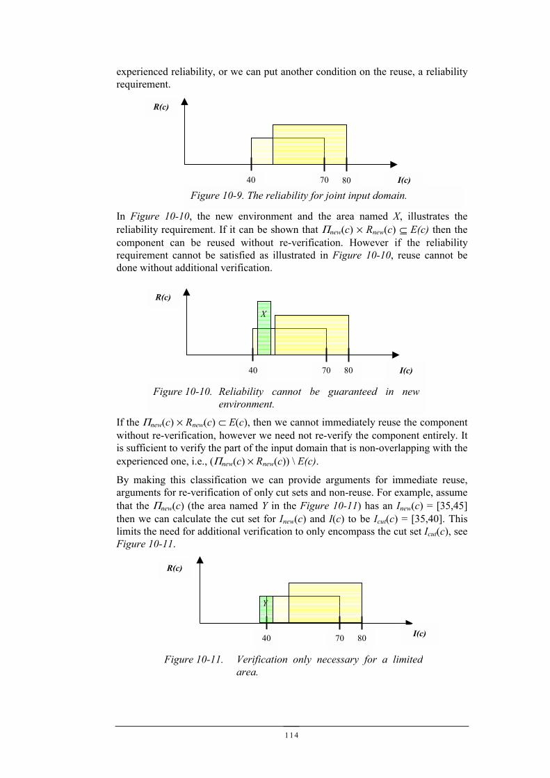
114

experienced reliability, or we can put another condition on the reuse, a reliabilityrequirement.

In Figure 10-10, the new environment and the area named X, illustrates thereliability requirement. If it can be shown that Πnew(c) × Rnew(c) ⊆ E(c) then thecomponent can be reused without re-verification. However if the reliabilityrequirement cannot be satisfied as illustrated in Figure 10-10, reuse cannot bedone without additional verification.

If the Πnew(c) × Rnew(c) ⊂ E(c), then we cannot immediately reuse the componentwithout re-verification, however we need not re-verify the component entirely. Itis sufficient to verify the part of the input domain that is non-overlapping with theexperienced one, i.e., (Πnew(c) × Rnew(c)) \ E(c).

By making this classification we can provide arguments for immediate reuse,arguments for re-verification of only cut sets and non-reuse. For example, assumethat the Πnew(c) (the area named Y in the Figure 10-11) has an Inew(c) = [35,45]then we can calculate the cut set for Inew(c) and I(c) to be Icut(c) = [35,40]. Thislimits the need for additional verification to only encompass the cut set Icut(c), seeFigure 10-11.

40 70 I(c)

R(c)

80

Figure 10-10. Reliability cannot be guaranteed in newenvironment.

X

R(c)

40 70 I(c)80

Figure 10-11. Verification only necessary for a limitedarea.

Y

40 70 I(c)

R(c)

80

Figure 10-9. The reliability for joint input domain.

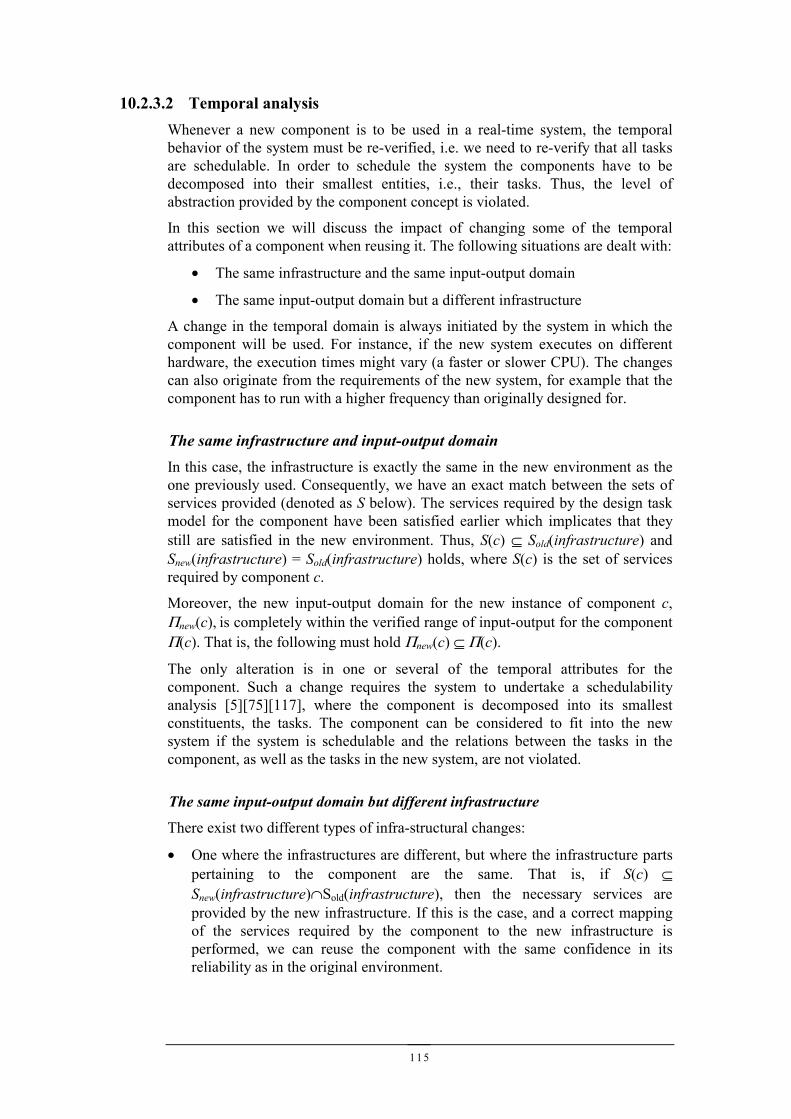
115

10.2.3.2 Temporal analysisWhenever a new component is to be used in a real-time system, the temporalbehavior of the system must be re-verified, i.e. we need to re-verify that all tasksare schedulable. In order to schedule the system the components have to bedecomposed into their smallest entities, i.e., their tasks. Thus, the level ofabstraction provided by the component concept is violated.

In this section we will discuss the impact of changing some of the temporalattributes of a component when reusing it. The following situations are dealt with:

• The same infrastructure and the same input-output domain

• The same input-output domain but a different infrastructure

A change in the temporal domain is always initiated by the system in which thecomponent will be used. For instance, if the new system executes on differenthardware, the execution times might vary (a faster or slower CPU). The changescan also originate from the requirements of the new system, for example that thecomponent has to run with a higher frequency than originally designed for.

The same infrastructure and input-output domainIn this case, the infrastructure is exactly the same in the new environment as theone previously used. Consequently, we have an exact match between the sets ofservices provided (denoted as S below). The services required by the design taskmodel for the component have been satisfied earlier which implicates that theystill are satisfied in the new environment. Thus, S(c) ⊆ Sold(infrastructure) andSnew(infrastructure) = Sold(infrastructure) holds, where S(c) is the set of servicesrequired by component c.

Moreover, the new input-output domain for the new instance of component c,Πnew(c), is completely within the verified range of input-output for the componentΠ(c). That is, the following must hold Πnew(c) ⊆ Π(c).

The only alteration is in one or several of the temporal attributes for thecomponent. Such a change requires the system to undertake a schedulabilityanalysis [5][75][117], where the component is decomposed into its smallestconstituents, the tasks. The component can be considered to fit into the newsystem if the system is schedulable and the relations between the tasks in thecomponent, as well as the tasks in the new system, are not violated.

The same input-output domain but different infrastructure

There exist two different types of infra-structural changes:

• One where the infrastructures are different, but where the infrastructure partspertaining to the component are the same. That is, if S(c) ⊆Snew(infrastructure)∩Sold(infrastructure), then the necessary services areprovided by the new infrastructure. If this is the case, and a correct mappingof the services required by the component to the new infrastructure isperformed, we can reuse the component with the same confidence in itsreliability as in the original environment.

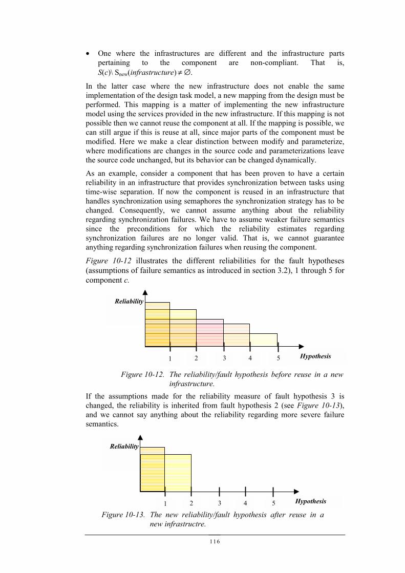
116

• One where the infrastructures are different and the infrastructure partspertaining to the component are non-compliant. That is,S(c)\ Snew(infrastructure) ≠ ∅.

In the latter case where the new infrastructure does not enable the sameimplementation of the design task model, a new mapping from the design must beperformed. This mapping is a matter of implementing the new infrastructuremodel using the services provided in the new infrastructure. If this mapping is notpossible then we cannot reuse the component at all. If the mapping is possible, wecan still argue if this is reuse at all, since major parts of the component must bemodified. Here we make a clear distinction between modify and parameterize,where modifications are changes in the source code and parameterizations leavethe source code unchanged, but its behavior can be changed dynamically.

As an example, consider a component that has been proven to have a certainreliability in an infrastructure that provides synchronization between tasks usingtime-wise separation. If now the component is reused in an infrastructure thathandles synchronization using semaphores the synchronization strategy has to bechanged. Consequently, we cannot assume anything about the reliabilityregarding synchronization failures. We have to assume weaker failure semanticssince the preconditions for which the reliability estimates regardingsynchronization failures are no longer valid. That is, we cannot guaranteeanything regarding synchronization failures when reusing the component.

Figure 10-12 illustrates the different reliabilities for the fault hypotheses(assumptions of failure semantics as introduced in section 3.2), 1 through 5 forcomponent c.

If the assumptions made for the reliability measure of fault hypothesis 3 ischanged, the reliability is inherited from fault hypothesis 2 (see Figure 10-13),and we cannot say anything about the reliability regarding more severe failuresemantics.

Reliability

2 4 Hypothesis51 3

Figure 10-12. The reliability/fault hypothesis before reuse in a newinfrastructure.

Reliability

2 4 Hypothesis51 3

Figure 10-13. The new reliability/fault hypothesis after reuse in anew infrastructre.

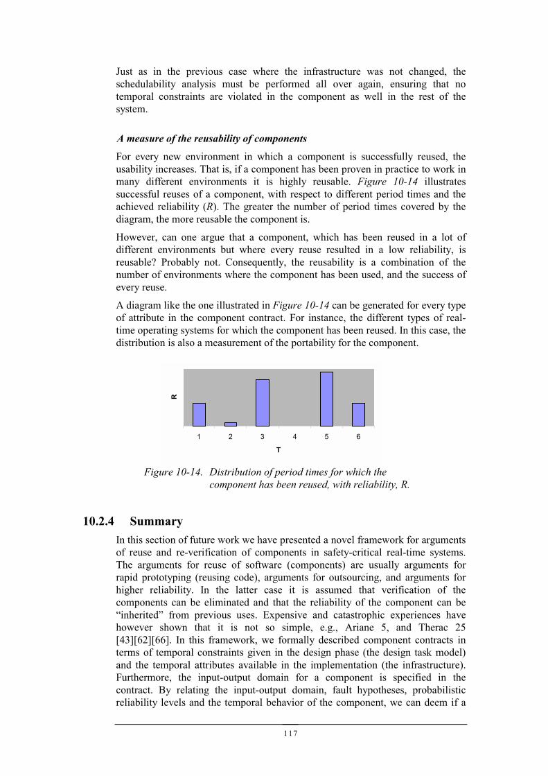
117

Just as in the previous case where the infrastructure was not changed, theschedulability analysis must be performed all over again, ensuring that notemporal constraints are violated in the component as well in the rest of thesystem.

A measure of the reusability of components

For every new environment in which a component is successfully reused, theusability increases. That is, if a component has been proven in practice to work inmany different environments it is highly reusable. Figure 10-14 illustratessuccessful reuses of a component, with respect to different period times and theachieved reliability (R). The greater the number of period times covered by thediagram, the more reusable the component is.

However, can one argue that a component, which has been reused in a lot ofdifferent environments but where every reuse resulted in a low reliability, isreusable? Probably not. Consequently, the reusability is a combination of thenumber of environments where the component has been used, and the success ofevery reuse.

A diagram like the one illustrated in Figure 10-14 can be generated for every typeof attribute in the component contract. For instance, the different types of real-time operating systems for which the component has been reused. In this case, thedistribution is also a measurement of the portability for the component.

10.2.4 SummaryIn this section of future work we have presented a novel framework for argumentsof reuse and re-verification of components in safety-critical real-time systems.The arguments for reuse of software (components) are usually arguments forrapid prototyping (reusing code), arguments for outsourcing, and arguments forhigher reliability. In the latter case it is assumed that verification of thecomponents can be eliminated and that the reliability of the component can be“inherited” from previous uses. Expensive and catastrophic experiences havehowever shown that it is not so simple, e.g., Ariane 5, and Therac 25[43][62][66]. In this framework, we formally described component contracts interms of temporal constraints given in the design phase (the design task model)and the temporal attributes available in the implementation (the infrastructure).Furthermore, the input-output domain for a component is specified in thecontract. By relating the input-output domain, fault hypotheses, probabilisticreliability levels and the temporal behavior of the component, we can deem if a

1 2 3 4 5 6

T

R

Figure 10-14. Distribution of period times for which thecomponent has been reused, with reliability, R.

118

component can be reused without re-verification or not. Of great significance isthat we can deem how much and which subsets, of say input-output domains, thatneed additional testing based on reliability requirements in the environment inwhich the reuse is intended. Faced with complete re-verification the possibility ofdecreasing the testing effort is attractive, and essential for safety-critical real-timesystems.

119

11 REFERENCES[1] Abdalla-Ghaly A. A. and Chan a. B. L. P. Y. Evaluation of competing reliability predictions.

IEEE Transactions on Software Engineering, pp. 950-967, 1986.[2] Alexander C. The Timeless Way of Building. Oxford University Press, 1979.[3] Alur R. and Dill D. A theory of timed automata. Theoretical Computer Science vol. 126 pp.

183-235, 1994.[4] Audsley N. C., Burns A., Davis R. I., Tindell K. W. Fixed Priority Pre-emptive Scheduling: A

Historical Perspective. Real-Time Systems journal, Vol.8(2/3), March/May, Kluwer A.P.,1995.

[5] Audsley N. C., Burns A., Richardson M.F., and Wellings A.J. Hard Real-Time Scheduling:The Deadline Monotonic Approach. Proc. 8th IEEE Workshop on Real-Time OperatingSystems and Software, pp. 127-132, Atlanta, Georgia, May, 1991

[6] Beizer B. Software testing techniques. Van Nostrand Reinhold, 1990.[7] Beugnard, Antoine, Jézéquel, Jean-Marc, Plouzeau, Noël and Watkins, Damien. Making

Component Contracts Aware. IEEE Computer July 1999, pp. 37-45.[8] Brantley W.C., MeAuliffe K.P. and Ngo T.A. RP3 performance monitoring hardware. In M.

Simmons, R. Koskela, and I. Bucher, eds. Instrumentation for Future Parallel ComputingSystems, pp. 35-45. Addison-Wesley, Reading, MA, 1989.

[9] Brooks F. P. No silver bullet – essence and accidents of software engineering. In informationprocessing 1986, the proceedings of the IFIP 10th world computing conference. H-J Kugler ed.Amsterdam: Elsevier Science, 1986, pp. 1069-1076.

[10] Butler, R.W. and Finelli, G.B. The infeasibility of quantifying the reliability of life-criticalreal-time software. IEEE Transactions on Software Engineering, (19): 3-12, January, 1993.

[11] Calvez J.P., and Pasquier O. Performance Monitoring and Assessment of Embedded HW/SWSystems. Design Automation for Embedded Systems journal, 3:5-22, Kluwer A.P., 1998.

[12] Chandy K. M. and Lamport L. Distributed snapshots: Determining global states of distributedsystems. ACM Trans. On Computing Systems, 3(1):63-75, February 1985.

[13] Chen J. and Burns A. Asynchronous Data Sharing in Muliprocessor Real-Time Systems UsingProcess Consensus. 10th Euromicro Workshop on Real-Time Systems, June 1998,

[14] Chodrow S.E, Jahanian F., and Donner M. Run-time monitoring of real-time systems. In Proc.of IEEE 12th Real-Time Systems Symposium, San Antonio, TX, pp. 74-83, December 1991.

[15] Ciupke O., Schmidt R. Components as Context-independent Units of Software. In Proc. ofECOOP, 1996.

[16] Clark G. and Powell A. Experiences with Sharing a Common Measurement Philosophy. InProceedings International Conference on Systems Engineering (INCOSE’99), Brighton, UK,1999.

[17] Clarke S.J. and McDermid JA. Software fault trees and weakest preconditions: a comparisonand analysis. Software Engineering Journal. 8(4):225-236, 1993.

[18] D’Souza D. F and Wills A. C. Objects, Components and Frameworks with UML. TheCatalysis Approach. Addison-Wesley, 1999.

[19] Dahl O.J, Dijskstra E.W., and Hoare C.A.R. Structured Programming. Academic Press, 1972.[20] DeMarco T. Structured Analysis and System Specification. Yourdon Press 1978. ISBN 0-

917072-07[21] DeMillo R. A., McCracken W.M., Martin R.J., and Passafiume J.F. Software Testing and

Evaluation. Benjamin/Cummings Publications. Co., 1987.[22] Dodd P. S., Ravishankar C. V. Monitoring and debugging distributed real-time programs.

Software-practice and experience. Vol. 22(10), pp. 863-877, October 1992.[23] E. Loyd and W. Tye. Systematic Safety: Safety Assessment of Aircraft Systems. Civil Aviation

Authority, London, England, 1982. Reprinted 1992.

120

[24] Ellis A. Achieving Safety in Complex Control Systems. Proceedings of the Safety-CriticalSystems Symposium. pp. 2-14. Brighton, England, 1995. Springr-Verlag. ISBN 3-540-19922-5

[25] Ellis W. J., Hilliard R.F., Poon P.T., Rayford D., Saunders T. F., Sherlund B., Wade R. L.,Toward a Recommended Practice for Architectural Description, Proceedings 2nd IEEEInternational Conference on Engineering of Complex Commuter Systems, Montreal, Quebec,Canada, October, 1996.

[26] Eriksson C., Mäki-Turja J., Post K., Gustafsson M., Gustafsson J., Sandström K., and BrorssonE. An Overview of RTT: A design Framework for Real-Time Systems. Journal of Parallel andDistributed Computing, vol. 36, pp. 66-80, Oct. 1996.

[27] Eriksson C., Thane H. and Gustafsson M. A Communication Protocol for Hard and Soft Real-Time Systems. In the proceedings of the 8th Euromicro Real-Time Workshop, L'Aquila Italy,June, 1996.

[28] Ferrari D. Consideration on the insularity of performance perturbations. IEEE Trans.Software Engineering, SE-16(6):678-683, June, 1986.

[29] Fidge, C. Fundamentals of distributed system observation. IEEE Software, (13):77 – 83,November, 1996.

[30] G J. Myers. The Art of Software Testing. John Wiley and Sons. New York 1979.[31] Gait J. A Probe Effect in Concurrent Programs. Software – Practice and Experience,

16(3):225-233, Mars, 1986.[32] Gamma E, Helm R., Johnson R., and Vlissides J. Design Patterns: Elements of Reusable

Object-Oriented Software. Addison Wesley, 1994.[33] Glass R. L. Real-time: The “lost world” of software debugging and testing. Communications

of the ACM, 23(5):264-271,May 1980.[34] Gorlick M. M. The flight recorder: An architectural aid for system monitoring. In Proc. of

ACM/ONR Workshop on Parallel and Distributed Debugging, Santa Cruz, CA, pp. 175-183,May 1991.

[35] Graham R. L. Bounds on Multiprocessing Timing Anomolies. SIAM journal of AppliedMathematics, 17(2), March, 1969.

[36] Haban D. and Wybranietz D. A Hyrbid monitor for behavior and performance analysis ofdistributed systems. IEEE Trans. Software Engineering, 16(2):197-211, February, 1990.

[37] Hamlet R. G. Probable Correctness Theory. Information processing letters 25, pp. 17-25,1987.

[38] Hatton L.. Unexpected (and sometimes unpleasant) Lessons from Data in Real SoftwareSystems. 12th Annual CSR Workshop, Bruges 12-15 September 1995. Proceedings, pp. 251-259. Springer. ISBN 3-540-76034-2.

[39] Helm R., Holland I. and Gangopadhyay D. Contracts: Specifying Behavioral Compositions inObject Oriented Systems. In Proc. of the Conference on Object Oriented Programming:Systems, Languages and Application, 1990.

[40] Hetzel B.. The Complete Guide to Software Testing. 2nd edition. QED Information Sciences,1988.

[41] Holland I. Specifying reusable components using contracts. In Proc. of ECOOP, 1992.[42] Hwang G.H, Tai K.C and Huang T.L. Reachability Testing: An Approach to Testing

Concurrent Software. Int. Journal of Software Engineering and Knowledge Engineering, vol.5(4):493-510, 1995.

[43] Inquiry Board. ARIANE 5 – Flight 50l Failure. Inquiry Board report,http://wxtnu.inria.fr/actualirdsfra.htrnl (July 1996), l8 p.

[44] Jelinski Z. and Moranda P. Software reliability research. In Statistical Computer PerformanceEvaluation (Frieberger W., ed.). New York: Academic Press.

[45] Joseph M. and Pandya P. Finding response times in a real-time system. The Computer Journal– British Computer Society, 29(5), pp.390-395, October, 1986.

[46] Joyce J., Lomow G., Slind K., and Unger B. Monitoring distributed systems. ACM Trans. OnComputer Systems, 5(2):121-150, May 1987.

121

[47] Keiller P. A. and Miller D. R. On the use and the performance of software reliability growthmodels. Reliability Engineering and System Safety, pp. 95-117, 1991.

[48] Knight J. C. and Leveson N. G. An experimental evaluation of the assumptions ofindependence in multiversion programming. IEEE Transactions on Software Engineering,vol. SE-12, pp. 96-109, Jan. 1986.

[49] Knight J. C. and N. G. Leveson. A reply to the criticism of the Knight and Leveson experiment.ACM SIGSOFT Software engineering Notes, 15, p. 25-35, January 1990.

[50] Kopetz H. and Grünsteidl H. TTP - A Protocol for Fault-Tolerant Real-Time Systems. IEEEComputer, January, 1994.

[51] Kopetz H. and Ochsenreiter W. Clock Synchronisation in Distributed Real-Time Systems.IEEE Trans. Computers, 36(8):933-940, Aug. 1987.

[52] Kopetz H. and Reisinger J. The Non-Blocking Write Protocol NBW: A Solution to a Real-Time Synchronization Problem. In Proceedings of he 14th Real-Time Systems Symposium, pp.131-137, 1993.

[53] Kopetz H. Sparse time versus dense time in distributed real-time systems. In the proceedingsof the 12th International Conference on Distributed Computing Systems, pp. 460-467, 1992.

[54] Kopetz H., Damm A., Koza Ch., Mulazzani M., Schwabl W., Senft Ch., and Zainlinger R..Distributed Fault-Tolerant Real-Time Systems: The MARS Approach. IEEE Micro, (9):25-40,1989.

[55] Kopetz H.. Event-Triggered versus Time-Triggered Real-Time Systems. Lecture Notes inComputer Science, vol. 563, Springer Verlag, Berlin, 1991.

[56] Kopetz, H. and Kim, K. Real-time temporal uncertainties in interactions among real-timeobjects. Proceedings of the 9th IEEE Symposium on Reliable Distributed Systems, Huntsville,AL, 1990.

[57] L Barroca and J McDermid. Formal Methods: Use and Relevance for Development of Safety-Critical Systems. The Computer Journal, Vol. 35, No. 6, 1992.

[58] Lamport L. Time, clock, and the ordering of events in a distributed systems. Comm. Of ACM,(21):558-565: July 1978.

[59] Laprie J.C. Dependability: Basic Concepts and Associated Terminology. DependableComputing and Fault-Tolerant Systems, vol. 5, Springer Verlag, 1992.

[60] Larsen K. G., Pettersson P. and Yi W. Uppaal in a Nutshell. In Springer International Journalof Software Tools for Technology Transfer 1(1+2), 1997.

[61] Lauterbach emulators. Lauterbach GmbH Germany. http://www.lauterbach.com/.[62] Le Lann, G. An analysis of the Ariane 5 flight 501 failure - a system engineering perspective.

Proceedings., International Conference and Workshop on Engineering of Computer-BasedSystems, pp. 339 - 346, 1997.

[63] LeBlanc T. J. and Mellor-Crummey J. M. Debugging parallel programs with instant replay.IEEE Trans. on Computers, C-36(4):471-482, April 1987.

[64] LeDoux C.H., and Parker D.S. Saving Traces for Ada Debugging. In the proceedings of Adaint. conf. ACM, Cambridge University press, pp. 97-108, 1985.

[65] Lee J.Y., Kang K.C.,Kim G.J., Kim H.J. Form the missing piece in effective real-time systemspecification and simulation. In proc. IEEE 4th Real-Time Technology and ApplicationsSymposium, pp.155 – 164, June 1998.

[66] Leveson N. and Turner C. An investigation of the Therac-25 accidents. IEEE Computer,26(7):18-41, July 1993.

[67] Leveson N. G. Safeware - System, Safety and Computers. Addison Wesley 1995. ISBN 0-201-11972-2.

[68] Leveson N. G. Software safety: What, why and How. ACM Computing surveys, 18(2),1986.[69] Littlewood B. and Keiller P. A. Adaptive software reliability modeling. In 14th International

Symposium on Fault-Tolerant Computing, pp. 108-113, IEEE Computer Society Press, 1984.[70] Littlewood B. and Strigini L. Validation of Ultrahigh Dependability for Software-based

Systems. Com. ACM, 11(36):69-80, November 1993.

122

[71] Littlewood B. Stochastic reliability-growth: A model for fault-removal in computer programsand hardware designs.' IEEE Transactions on Reliability, pp. 313-320, 1981.

[72] Littlewood B.and Verrall. A Bayesian Reliability Growth Model For Computer Software.Journal of the Royal Statistical Society, Series C, No. 22, p 332-346, 1973

[73] Liu A.C. and Parthasarathi R. Hardware monitoring of a multiprocessor systems. IEEE Micro,pp. 44-51, October 1989.

[74] Lozzerini B., Prete C. A., and Lopriore L. A programmable debugging aid for real-timesoftware development. IEEE Micro, 6(3):34-42, June 1986.

[75] Lui C. L. and Layland J. W.. Scheduling Algorithms for multiprogramming in a hard real-time environment. Journal of the ACM 20(1), 1973.

[76] Lutz R. R.. Analyzing software requirements errors in safety-critical, embedded systems. Insoftware requirements conference, IEEE, January 1992.

[77] Malony A. D., Reed D. A., and Wijshoff H. A. G. Performance measurement intrusion andperturbation analysis. IEEE Trans. on Parallel and Distributed Systems 3(4):433-450, July1992.

[78] McDowell C.E. and Hembold D.P. Debugging concurrent programs. ACM ComputingSurveys, 21(4), pp. 593-622, December 1989.

[79] Mellor-Crummey J. M. and LeBlanc T. J. A software instruction counter. In Proc. of 3dInternational Conference on Architectural Support for Programming Languages and OperatingSysterns, Boston, pp. 78-86, April 1989

[80] Miller B.P., Macrander C., and Sechrest S. A distributed programs monitor for BerkeleyUNIX. Software Practice and Experience, 16(2):183-200, February 1986.

[81] Mink K., Carpenter R., Nacht G., and Roberts J. Multiprocessor performance measurementinstrumentation. IEEE Computer, 23(9):63-75, September 1990.

[82] Mäki-Turja J., Fohler G. and Sandström K. Towards Efficient Analysis of Interrupts in Real-Time Systems. In proceedings of the 11th EUROMICRO Conference on Real-Time Systems,York, England, May 1999.

[83] Netzer R.H.B. and Xu Y. Replaying Distributed Programs Without Message Logging. In proc.6th IEEE Int. Symposium on High Performance Distributed Computing. Pp. 137-147. August1997.

[84] Neuman P G. Computer Related Risks. ACM Press, Adison-Wesley, 1995. ISBN 0-201-55805-x.

[85] Parnas D.L., van Schouwen J., and Kwan S.P. Evaluation of Safety-Critical Software.Communication of the ACM, 6(33):636-648, June 1990.

[86] Plattner B. Real-time execution monitoring. IEEE Trans. Software Engineering, 10(6), pp.756-764, Nov., 1984.

[87] Poledna S. Replica Determinism in Distributed Real-Time Systems: A Brief Survey. Real-Times systems Journal, Kluwer A.P., (6):289-316, 1994.

[88] Powell D. Failure Mode Assumptions and Assumption Coverage: In Proc. 22nd InternationalSymposium on Fault-Tolerant Computing. IEEE Computer Society Press, pp.386-395, July,1992.

[89] Puschner P. and Koza C. Calculating the maximum execution time of real-time programs.Journal of Real-time systems, Kluwer A.P., 1(2):159-176, September, 1989.

[90] Raju S. C. V., Rajkumar R., and Jahanian F. Monitoring timing constraints in distributed real-time systems. In Proc. of IEEE 13th Real-Time Systems Symposium, Phoenix, AZ, pp. 57-67,December 1992.

[91] Reilly M. Instrumentation for application performance tuning: The M3l system. In SimmonsM., Koskela R., and Bucher I., eds. Instrumentation for Future Parallel Computing Systems,pp. 143-158. Addison-Wesley, Reading, MA, 1989.

[92] Rothermel G. and Harrold M.J. Analyzing regression test selection techniques. IEEE trans.Software Engineering. 8(22):529-551. August 1996.

123

[93] Rushby J. Formal methods and their Role in the Certification of Critical Systems. Proc. 12th

Annual Center for Software Reliability Workshop, Bruges 12-15 Sept. 1995, pp. 2-42.Springer Verlag. ISBN 3-540-76034-2.

[94] Rushby J., Formal Specification and Verification for Critical systems: Tools, Achievements,and prospects. Advances in Ultra-Dependable Distributed Systems. IEEE Computer SocietyPress. 1995. ISBN 0-8186-6287-5.

[95] Sandström K., Eriksson C., and Fohler G. Handling Interrupts with Static Scheduling in anAutomotive Vehicle Control System. In proceedings of the 5th Int. Conference on Real-TimeComputing Systems and Applications (RTCSA’98). October 1998, Japan.

[96] Schütz W. Fundamental Issues in Testing Distributed Real-Time Systems. Real-Time Systemsjournal, vol. 7(2): 129-157, Kluwer A.P., 1994.

[97] Schütz W. Real-Time Simulation in the Distributed Real-Time System MARS. In proc.European Simulation Multiconference 1990, Erlangen, BRD, June 1990.

[98] Shaw M., Clements P., A field guide to boxology: preliminary classification of architecturalstyles. In proc. 21st Annual International Computer Software and Applications Conference,1997 (COMPSAC '97). ISBN: 0-8186-8105-5.

[99] Shimeall T. J. and Leveson N. G. An empirical comparison of software fault-tolerance andfault elimination. IEEE Transactions on Software Engineering, pp. 173-183, Feb. 1991.

[100] Shin K. G. HARTS: A distributed real-time architecture. IEEE Computer, 24(5), pp. 25-35,May, 1991.

[101] Sifakis J. and Yovine S. Compositional specification of timed systems. In Proc. 13th AnnualSymposium on Theoretical Aspects of Computer Science, STACS'96, Grenoble, France,Lecture Notes in Computer Science 1046, pp. 347-359. Springer Verlag, February 1996.

[102] Sommerville I. Software Engineering. Addison-Wesley, 1992. ISBN 0-201-56529-3.[103] Szyperski C. Component Software - Beyond Object-Oriented Programming. Addison-Wesley,

1997.[104] Tai K.C, Carver R.H., and Obaid E.E. Debugging concurrent Ada programs by deterministic

execution. IEEE transactions on software engineering. Vol. 17(1), pp. 45-63, January 1991.[105] Thane H. and Hansson H. Handling Interrupts in Testing of Distributed Real-Time Systems. In

proc. Real-Time Computing Systems and Applications conference (RTCSA’99), Hong Kong,December, 1999.

[106] Thane H. and Hansson H. Towards Systematic Testing of Distributed Real-Time Systems. Proc.20th IEEE Real-Time Systems Symposium, Phoenix, Arizona, December 1999.

[107] Thane H. and Hansson H. Using Deterministic Replay for Debugging of Distributed Real-Time Systems. In proceedings of the 12th Euromicro Conference on Real-Time Systems(ECRTS’00), Stockholm, June 2000.

[108] Thane H. Asterix the T-REX among real-time kernels. Timely, reliable, efficient andextraordinary. Technical report in preparation, Mälardalen Real-Time Research Centre, Dept.Computer Engineering, Mälardalen University, 2000

[109] Thane H. Design for Deterministic Monitoring of Distributed Real-Time Systems. Technicalreport, Mälardalen Real-Time Research Centre, Dept. Computer Engineering, MälardalenUniversity, 1999.

[110] Tindell K. W., Burns A., and Wellings A.J. Analysis of Hard Real-Time Communications.Journal of Real-Time Systems, vol. 9(2), pp.147-171, September 1995.

[111] Tokuda H., Kotera M., and Mercer C.W. A Real-Time Monitor for a Distributed Real-TimeOperating System. In proc. of ACM Workshop on Parallel and Distributed Debugging,Madison, WI, pp. 68-77, May, 1988.

[112] Tsai J.P., Bi Y.-D., Yang S., and Smith R.. Distributed Real-Time System: Monitoring,Visualization, Debugging, and Analysis. Wiley-Interscience, 1996. ISBN 0-471-16007-5.

[113] Tsai J.P., Fang K.-Y., Chen H.-Y., and Bi Y.-D. A Noninterference Monitoring and ReplayMechanism for Real-Time Software Testing and Debugging. IEEE Trans. on Software Eng.vol. 16, pp. 897 - 916, 1990.

[114] Voas J M and Freidman. Software Assessment: Reliability, Safety, testability. WileyInterscience, 1995. ISBN 0-471-01009-x.

124

[115] Voas J. and Miller. Designing Programs that are Less Likely to Hide Faults. Journal ofSystems Software, 20:93-100, 1993,

[116] Voas J. PIE: A dynamic Failure Based Technique. IEEE Transactions on SoftwareEngineering, vol. 18(8), Aug. 1992.

[117] Xu J. and Parnas D. Scheduling processes with release times, deadlines, precedence, andexclusion, relations. IEEE Trans. on Software Eng. 16(3):360-369, 1990.

[118] Yang R-D and Chung C-G. Path analysis testing of concurrent programs. Information andsoftware technology. vol. 34(1), January 1992.