MSSM with Non-holomorphic Soft Interactions

Utpal Chattopadhyay,School of Physical Sciences,

Indian Association for the Cultivation of Science,Kolkata, India

[Ref.: UC, Abhishek Dey, JHEP 1610 (2016) 027, arXiv:1604.06367],[UC, AseshKrishna Datta, Samadrita Mukherjee, Abhaya Kumar Swain, JHEP

1810 (2018) 202, arXiv: 1809.05438]IMHEP 2019, IOP, Bhubaneswar, January 17, 2019

1 / 28

MSSMI MSSM Superpotential and soft SUSY breaking terms::

W = µHD .HU − Y eij HD .Li Ej − Y d

ij HD .Qi Dj − Y uij Qi .HU Uj

A.B = εαβAαBβ

−Lsoft = [qiL.hu(Au)ij u∗jR + hd .qiL(Ad)ij d

∗jR + hd .liL(Ae)ij e

∗jR + h.c.]

+ (Bµhd .hu + h.c.) + m2d |hd |2 + m2

u|hu|2

+ q∗iL(M2q )

ij+ u∗iR(M2

u )ij ujR + d∗iR(M2d )

ijdjR + l∗iL(M2

l )ijljL

+ gaugino mass terms

I Possible origin of soft terms: SUSY breaking parametrized by vev ofF -term of a chiral superfield X , so that < X >= θθ < F >≡ θθF . Xcouples to Φ and a gauge strength superfield W a

α.

Type Term Naive Suppression Origin

φφ∗ |F |2M2 ∼ m2

W1

M2 [XX ∗ΦΦ∗]Dsoft φ2 µF

M∼ µmW

µM

[XΦ2]Fφ3 F

M∼ mW

1M

[XΦ3]Fλλ F

M∼ mW

1M

[XW αWα]F

I Are there any more possible soft terms ?

2 / 28

Nonholomorphic soft SUSY breaking termsI S. Martin, Phys. Rev D., 2000; Possible non-holomorphic soft SUSY breaking terms:

Type Term Naive Suppression Origin

φ2φ∗ |F |2M3 ∼

m2WM

1M3 [XX ∗Φ2Φ∗]D

“maybe soft” ψψ |F |2M3 ∼

m2WM

1M3 [XX ∗DαΦDαΦ]D

ψλ |F |2M3 ∼

m2WM

1M3 [XX ∗DαΦWα]D

I “maybe soft”: In the absence of any gauge singlet scalar the abovenon-holomorphic terms are of soft SUSY breaking in nature. But, thesehave mass scale suppression by M.

I A gauge singlet scalar field would have tadpole contributions causinghard SUSY breaking.

I NHSSM: MSSM + NH terms like φ2φ∗ and ψψ:

−L′soft = hcd .qiL(A′u)ij u

∗jR + qiL.h

cu(A′d)ij d

∗jR + liL.h

cu(A′e)ij e

∗jR + µ′hu.hd + h.c.

Higgs fields are replaced with their conjugates: hd going with up-type ofsquarks etc.

I VHiggs is unaffected. But, the potential involving charged and coloredscalar fields needs a separate study for CCB.

3 / 28

Nonholomorphic terms: A partial list of related

analyses and our present workI Hall and Randall, PRL 1990, Jack and Jones, PRD 2000: Quasi IF fixed points

and RG invariant trajectories; Jack and Jones PLB 2004: General analyses withNH terms involving RG evolutions.

I Works performed under Constrained MSSM (CMSSM)/minimalsupergravity(mSUGRA) setup for studying the Higgs mass and observables likeBr(B → Xs + γ) etc.: Hetherington JHEP 2001, Solmaz et. al. PRD 2005,PLB 2008, PRD 2015. The analyses involve mixed type of inputs given at theunification and electroweak scales.

I Ross, Schmidt-Hoberg, Staub PLB 2016, JHEP 2017. Focused on fine-tuningand higgsino DM, stressed the importance of the bilinear higgsino termidentifying various scenarios.

I UC, A. Dey JHEP 2016: No specific mechanism for SUSY breaking: all theparameters are given at the low scale. Impact on muon g − 2 apart from EWfine-tuning, Higgs mass etc.UC, D. Das, S. Mukherjee, JHEP 2018: On GMSB type of realization ofNHSSM.J. Beuria and A. Dey, JHEP 2017, CCB effects in NHSSMUC, A. Datta, S. Mukherjee, A. K. Swain: JHEP 2018, Sbottomphenomenology.

4 / 28

Bilinear Higgsino soft term

I The following reparametrization of µ, µ′ and Higgs scalar massparameters may evade the need of a bilinear higgsino soft term.µ→ µ+ δ, µ′ → µ′ + δ, and m2

HU,D→ m2

HU,D− 2µδ − δ2

I A reparametrization would however involve ad-hoc correlations betweenunrelated parameters [Jack and Jones 1999, Hetherington 2001 etc.].

I Such correlations are arbitrary, at least in view of fine-tuning. Inparticular, there may be a scenario where definite SUSY breakingmechanisms generate bilinear higgsino soft terms whereas it may keepthe scalar sector unaffected. [Ross et. al. 2016, 2017, Antoniadis et. al. 2008, Perez et. al.2008 etc].

I The µ′ term that is traditionally retained, isolates a fine-tuning measure(typically ∼ factor× µ2/M2

Z ) from the higgsino mass (µ+ µ′): ⇒Possibility of a large higgsino mass (like a TeV satisfying DM relic limits)while having a small fine-tuning.

In a general standpoint we acknowledge the importance of trilinear and bilinearNH soft terms, irrespective of a suppression predicted by a given model. Unlikeother analyses, we will use a pMSSM type of work on Non-holomorphicsupersymmetric SM (NHSSM).

5 / 28

NHSSM: scalars and electroweakinosI

Squarks : M2u =

m2Q

+ ( 12− 2

3sin2 θW )M2

Z cos 2β + m2u −mu(Au − (µ + A′u) cot β)

−mu(Au − (µ + A′u) cot β) m2u + 2

3sin2 θWM2

Z cos 2β + m2u

,Sleptons (off-diagonal): −mµ[Aµ − (µ + A′µ) tan β]⇒ A′µ tan β potentially enhances (g − 2)SUSY

µ ,

particularly affecting the χ01 − µ loop contributions.

I

Higgs mass corrections :∆m2h,top =

3g22 m

4t

8π2M2W

ln

(mt1

mt2

m2t

)+

X 2t

mt1mt2

1−X 2t

12mt1mt2

,Here, Xt = At − (µ + A′t ) cot β ⇒ influence on mh .

I

Charginos : Mχ± =

M2√

2MW sin β√

2MW cos β −(µ + µ′)

,mχ±1

>∼ 100 GeV⇒ |µ + µ′| >∼ 100 GeV. Muon g − 2 may be enhanced via a light higgsino.

I

Neutralinos : Mχ0 =

M1 0 −MZ cos β sin θW MZ sin β sin θW

0 M2 MZ cos β cos θW −MZ sin β cos θW

−MZ cos β sin θW MZ cos β cos θW 0 −(µ + µ′)

MZ sin β sin θW −MZ sin β cos θW −(µ + µ′) 0

.

I If |(µ + µ′)| << M1,M2 ⇒ χ01 is higgsino-like. It is possible to have an acceptable higgsino-like LSP

with small µ (∼ i.e. small electroweak fine-tuning.)6 / 28

Muon anomalous magnetic moment: (g − 2)µ in

MSSMI Large discrepancy from the SM (more than 3σ): aexpµ − aSMµ = (29.3± 8)× 10−10

I MSSM contributions to muon (g-2): Diagrams involving charginos and neutralinos

Gauge Eigenstate basis:. .

˜W− ˜H−

µL µRνµ(a)

˜B

µL µL

m2LR

µR µR

(b)

˜B˜H0

µL µRµL

(c)

˜W 0 ˜H0

µL µRµL

(d)

˜H0 ˜B

µL µRµR

(e)

I Slepton L-R mixing in MSSM:mµ(Aµ − µ tan β)

I The mixing influences the last item of ∆aµshown in blue. Typically, Aµ is quite smallerthan µ tan β, especially for large tan β.

I In NHSSM: mµ[(Aµ−A′µ tan β)−µ tan β]

A′µ effect is enhanced by tan β causing a

significant change in ∆aµ.

∆aµ(W , H, νµ) ' 15 × 10−9(

tan β

10

)((100 GeV)2

M2µ

)(fC

1/2

),

∆aµ(W , H, µL) ' −2.5 × 10−9(

tan β

10

)((100 GeV)2

M2µ

)(fN

1/6

),

∆aµ(B, H, µL) ' 0.76× 10−9(

tan β

10

)((100 GeV)2

M1µ

)(fN

1/6

),

∆aµ(B, H, µR ) ' −1.5 × 10−9(

tan β

10

)((100 GeV)2

M1µ

)(fN

1/6

),

∆aµ(µL, µR , B) ' 1.5 × 10−9(

tan β

10

) (100 GeV)2

m2µL

m2µR/M1µ

( fN

1/6

).

[Ref. arXiv 1303.4256 by Endo, Hamaguchi, Iwamoto,Yoshinaga]

7 / 28

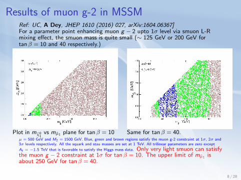
Results of muon g-2 in MSSMRef: UC, A Dey, JHEP 1610 (2016) 027, arXiv:1604.06367]For a parameter point enhancing muon g − 2 upto 1σ level via smuon L-Rmixing effect, the smuon mass is quite small (∼ 125 GeV or 200 GeV fortanβ = 10 and 40 respectively.)

Plot in mχ01

vs mµ1 plane for tanβ = 10 Same for tanβ = 40.µ = 500 GeV and M2 = 1500 GeV. Blue, green and brown regions satisfy the muon g-2 constraint at 1σ, 2σ and3σ levels respectively. All the squark and stau masses are set at 1 TeV. All trilinear parameters are zero except

At = −1.5 TeV that is favorable to satisfy the Higgs mass data. Only very light smuon can satisfythe muon g − 2 constraint at 1σ for tanβ = 10. The upper limit of mµ1 isabout 250 GeV for tanβ = 40.

8 / 28

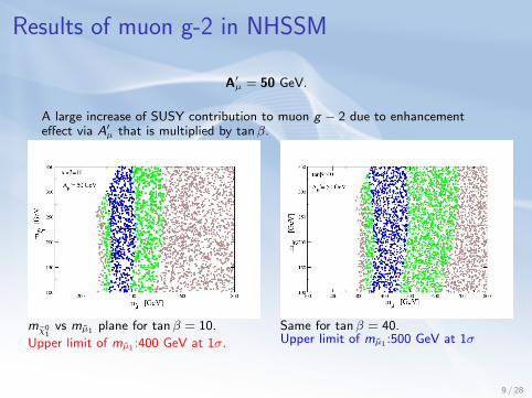
Results of muon g-2 in NHSSM

A′µ = 50 GeV.

A large increase of SUSY contribution to muon g − 2 due to enhancementeffect via A′µ that is multiplied by tanβ.

mχ01

vs mµ1 plane for tanβ = 10.

Upper limit of mµ1 :400 GeV at 1σ.

Same for tanβ = 40.Upper limit of mµ1 :500 GeV at 1σ

9 / 28

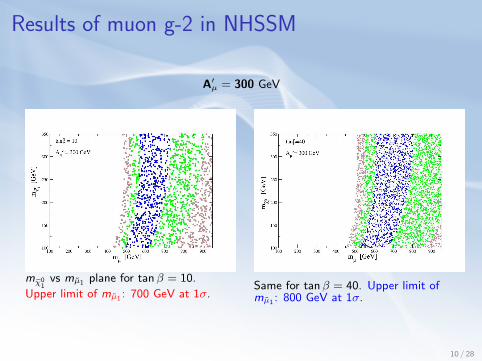
Results of muon g-2 in NHSSM

A′µ = 300 GeV

mχ01

vs mµ1 plane for tanβ = 10.

Upper limit of mµ1 : 700 GeV at 1σ.Same for tanβ = 40. Upper limit ofmµ1 : 800 GeV at 1σ.

10 / 28

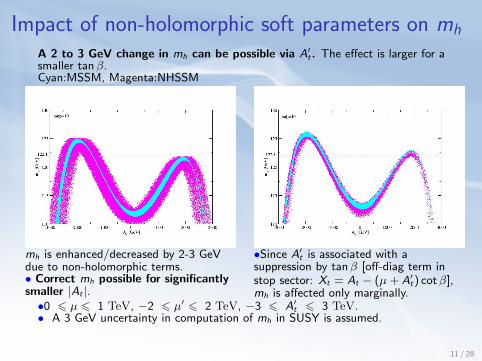
Impact of non-holomorphic soft parameters on mh

A 2 to 3 GeV change in mh can be possible via A′t . The effect is larger for asmaller tanβ.Cyan:MSSM, Magenta:NHSSM

mh is enhanced/decreased by 2-3 GeVdue to non-holomorphic terms.• Correct mh possible for significantlysmaller |At |.

•Since A′t is associated with asuppression by tanβ [off-diag term instop sector: Xt = At − (µ+ A′t) cotβ],mh is affected only marginally.

•0 6 µ 6 1 TeV, −2 6 µ′ 6 2 TeV, −3 6 A′t 6 3 TeV.• A 3 GeV uncertainty in computation of mh in SUSY is assumed.

11 / 28

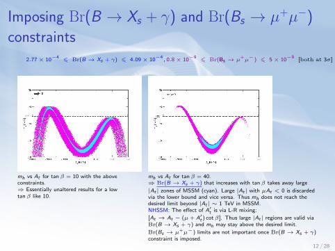
Imposing Br(B → Xs + γ) and Br(Bs → µ+µ−)

constraints2.77× 10−4 6 Br(B → Xs + γ) 6 4.09× 10−4

, 0.8× 10−9 6 Br(Bs → µ+µ−) 6 5× 10−9 [both at 3σ]

mh vs At for tan β = 10 with the aboveconstraints.⇒ Essentially unaltered results for a lowtan β like 10.

mh vs At for tan β = 40.⇒ Br(B → Xs + γ) that increases with tan β takes away large

|At | zones of MSSM (cyan). Large |At | with µAt < 0 is discardedvia the lower bound and vice versa. Thus mh does not reach thedesired limit beyond |At | ∼ 1 TeV in MSSM.NHSSM: The effect of A′t is via L-R mixing:

[At → At − (µ + A′t ) cot β]. Thus large |At | regions are valid viaBr(B → Xs + γ) and mh may stay above the desired limit.

Br(Bs → µ+µ−) limits are not important once Br(B → Xs + γ)constraint is imposed.

12 / 28

Electroweak fine-tuning in MSSM

EWSB conditions out of minimization of VHiggs :

m2Z

2=

m2Hd−m2

Hutan2 β

tan2 β − 1− |µ|2, sin 2β =

2b

m2Hd

+ m2Hu

+ 2|µ|2

(1)

Electroweak Fine-tuning:

∆pi =

∣∣∣∣∣∂ lnm2

Z (pi )

∂ ln pi

∣∣∣∣∣ , ∆Total =

√∑i∆2

pi,where pi ≡ µ2, b,mHu ,mHd

I For tanβ and µ both not too small the most important term is ∆(µ) ' 4µ2

m2Z

.

For a moderately large tanβ, a small µ means a small ∆Total .

I NH soft terms do not contribute to VHiggs at the tree level. Possibility of smallµ with a larger higgsino LSP mass ∼ |µ+ µ′| satisfying the DM data (as asingle component one). This is unlike MSSM.

13 / 28

Probing NHSSM via sbottom decay at the LHC: Outline

Ref: UC, AseshKrishna Datta, Samadrita Mukherjee, Abhaya Kumar Swain,JHEP 1810 (2018) 202, arXiv: 1809.05438

I b1 pair production and decay leading to 2b + /ET via b1 → b + χ01. Other

decay modes can be b1 → t + χ−1 and b1 → t1 + W−. Kinematic

elimination used for b1 → t1 + W−.

I Higgsino dominated χ01 (µ ≤ 350 GeV) is generally considered for

naturalness. µ′ = 0 is chosen in the main body of the analysis forsimplicity.

I We keep the left and the right mass parameters mbLand mbR

to be the

same. ⇒ For no mixing, b1 and b2 are very close to L and R likerespectively with effectively equal masses. With Ab = 0, mixing occursvia (µ+ A′b) that itself is associated with a tanβ enhancement.

I A significant amount of radiative correction may change yb in NHSSM.This, not only may affect the L-R mixing but may also change couplingsconcerned with the above electroweakinos and quarks in the bi decaymodes.

I Parton-level yields for (σb1 b1×BR[b1 → bχ0

1]2) in the final state 2b + /ET

arising from pair-produced b1 at the 13 TeV run are compared forNHSSM and MSSM for varying A′b. Parameter space explored for largeyield ratios.

14 / 28

Outline contd.

I Analysis is extended to involve b2. Comparison made with MSSM withproper ratio of yields involving b1 and b2 pair productions and decay into2b + /ET .

I Analysis is extended to varying mbLand mbR

.

I Implications on stop searches are probed in relation to appearance oflarge yb via radiative effects that may affect t1 → bχ+

1 .

Stepwise analysis involves understanding how the relevant couplings behavewhile A′b changes. Consequently, one investigates how the branching ratiosBr(b1 → b + χ0

1) and Br(b1 → t + χ±1 ) are affected and finally how the yieldsvary for changing A′b.

15 / 28

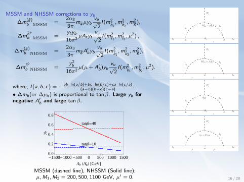
MSSM and NHSSM corrections to yb

∆m(g)b MSSM

=2α3

3πmgµyb

vu√2I (m2

b1,m2

b2,m2

g ),

∆mh+

b MSSM =ytyb

16π2µAtyt

vu√2I (m2

t1,m2

t2, µ2) ,

∆m(g)b NHSSM

=2α3

3πmgA

′byb

vu√2I (m2

b1,m2

b2,m2

g ),

∆mh0

b NHSSM =y2b

16π2µ(µ+ A′b)yb

vu√2I (m2

b1,m2

b2, µ2).

where, I (a, b, c) = − ab ln(a/b)+bc ln(b/c)+ca ln(c/a)(a−b)(b−c)(c−a)

.

• ∆mb(or ∆yb) is proportional to tanβ. Large yb fornegative A′b and large tanβ.

tanβ=10

tanβ=40

-1500-1000 -500 0 500 1000 1500

0.0

0.2

0.4

0.6

0.8

Ab (Ab ) [GeV]

y b

MSSM (dashed line), NHSSM (Solid line);µ,M1,M2 = 200, 500, 1100 GeV, µ′ = 0.

bL bR

bLbR

H∗u

g g

mg

M 2LR = µyb

×gs gs

bL bR

tRtL

Hu

h± h±µ

M 2LR ≃ Atyt

×

bL bR

bLbR

H∗u

g g

mg

A′byb

×gs gs

bL bR

bRbL

H∗u

χ01 χ0

1

µ

(µ + A′b)yb

×

16 / 28

Sbottom-electroweakino couplings

The decay rates will essentially beproportional to C2

L + C2R where CL,CR

appear in the expression for couplings asgiven below.For bi -b-χ0

1 coupling:

CL = − i

6(−3√

2g2N∗12Z

di3 + 6N13ybZ

di6

+√

2g1N11Zdi3),

CR = − i

3(3ybZ

di3N13 +

√2g1Z

di6N11).

For bi -t-χ−1 coupling:

CL = i(ytZdi3V12),

CR = i(−g2U∗11Z

di3 + U∗12ybZ

di6).

Nij are elements of neutralino diagonalizingmatrix elements. N13,N14 will be large forhiggsino dominated LSP. Zij ’s are forsquark diagonalizing matrix elementswhere large Zi3 and Zi6 would mean largeL and R-components in bi for i = 1, 2.

I We consider higgsino like χ01 and

χ±1 .

I For bi → bχ01 both CL and CR are

approximately proportional to yb.

I For bi → tχ−1 , couplings for L-type

bi is ∝ yt whereas for R-like bicoupling will be ∝ yb.

I A left like bi will largely decay viatχ−1 . Thus it will have a smallerBranching fraction for bχ0

1,2.

I NHSSM for non-vanishing A′b maybe associated with a large yb andthis will cause a significantlydifferent behaviour with respect toMSSM.

I We ignored b1 → t1W−

kinematically by the choice ofmb1

< mt1+ mW .

17 / 28

Sbottom-electroweakino couplings

For bi -b-χ01 coupling:

CL = −i

6(−3√

2g2N∗12Z

di3 + 6N13ybZ

di6

+√

2g1N11Zdi3),

CR = −i

3(3ybZ

di3N13 +

√2g1Z

di6N11).

For bi -t-χ−1 coupling:

CL = i(ytZdi3V12),

CR = i(−g2U∗11Z

di3 + U∗12ybZ

di6).

I Spread appears due to 100 < µ < 350 GeV.Region around µ+ A′b ' 0 refers to scenarios of

b1, b2 to be Left and Right like with negligiblemixing. Large non-vanishing A′b zones refer tolarger mixing.

I For bi → bχ01, a change of sign of Zd

13 occursnear the no mixing zone. ybenhancement/suppression occurs fornegative/positive A′b especially for large tan β.

I For bi → tχ−1 , the central region for b1 is Leftlike, henced peaked due to yt irrespective oftan β. For large negative A′b and large tan β ybenhancement effect is seen in the left zone. Forthe small tan β case, yt dominates over yb .

18 / 28

Branching ratios

tanβ=10

tanβ=40

-1500-1000 -500 0 500 1000 1500

0.0

0.2

0.4

0.6

0.8

Ab (Ab ) [GeV]

y b

I Br(b1 → bχ01) essentially follows the

profile of the couplings.

I When b1 is left dominated (centralregion) the b1 → tχ−1 decay rate isdriven by yt , hence becomes large.

I Difference of rates gets smaller forincrease in yb i.e. large negative A′band large tanβ cases wherecompetition sets in between themodes.

19 / 28

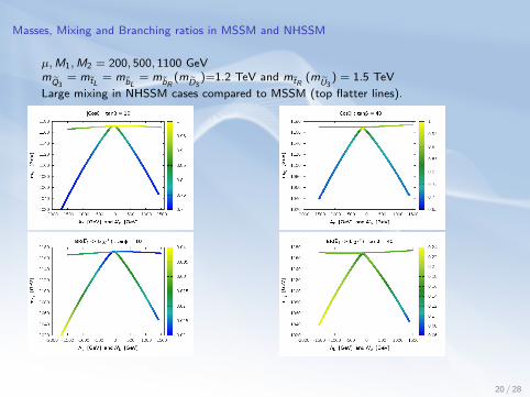
Masses, Mixing and Branching ratios in MSSM and NHSSM

µ,M1,M2 = 200, 500, 1100 GeVm

Q3= mtL

= mbL= mbR

(mD3

)=1.2 TeV and mtR(m

U3) = 1.5 TeV

Large mixing in NHSSM cases compared to MSSM (top flatter lines).

20 / 28

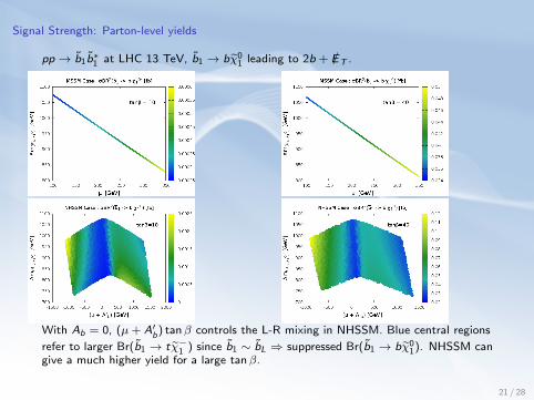
Signal Strength: Parton-level yields

pp → b1b∗1 at LHC 13 TeV, b1 → bχ01 leading to 2b + /ET .

With Ab = 0, (µ+ A′b) tanβ controls the L-R mixing in NHSSM. Blue central regions

refer to larger Br(b1 → tχ−1 ) since b1 ∼ bL ⇒ suppressed Br(b1 → bχ01). NHSSM can

give a much higher yield for a large tanβ.

21 / 28

Ratio of yields for b1

100 < µ < 350 GeV and |A′b| < 1.2 TeV.

α1(A′b) =

[(σb1 b1

× BR[b1 → bχ01]2)]NHSSM

[(σb1 b1

× BR[b1 → bχ01]2)]MSSM

Ratio α1 refers to same value of µ for MSSM and NHSSM. There is about an 8-foldincrease from the lowest to the highest value for tanβ = 10 and around a 6-foldincrease for tanβ = 40. Largest regions of α1 fall in the negative large A′b zone due toyb-enhancement.

22 / 28

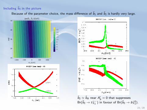
Including b2 in the picture

Because of the parameter choice, the mass difference of b1 and b2 is hardly very large.

-1000 -500 0 500 1000

10

20

30

40

50

A'b [GeV]

tanβ

Δm(b2 , b

1) [GeV]

20

40

60

80

100

120

140

160

180

b2 ' bR near A′b = 0 that suppresses

Br(b2 → tχ−1 ) in favour of Br(b2 → bχ01).

23 / 28

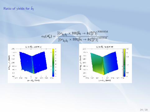
Ratio of yields for b2

α2(A′b) =

[(σb2 b2

× BR[b2 → bχ01]2)]NHSSM

[(σb2 b2

× BR[b2 → bχ01]2)]MSSM

24 / 28

Ratio of yields for b1 plus b2

αtotal(A′b) =

∑i=1,2

[(σbi bi

× BR[bi → bχ01]2)]NHSSM

∑i=1,2

[(σbi bi

× BR[bi → bχ01]2)]MSSM

Up to eight-fold (six-fold) increased rates could be possible for tanβ = 10 (40) overthe expected MSSM rates in the final state under consideration.

25 / 28

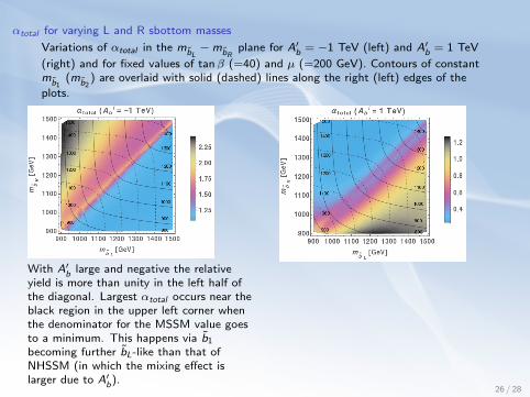
αtotal for varying L and R sbottom masses

Variations of αtotal in the mbL−mbR

plane for A′b = −1 TeV (left) and A′b = 1 TeV

(right) and for fixed values of tanβ (=40) and µ (=200 GeV). Contours of constantmb1

(mb2) are overlaid with solid (dashed) lines along the right (left) edges of the

plots.

With A′b large and negative the relativeyield is more than unity in the left half ofthe diagonal. Largest αtotal occurs near theblack region in the upper left corner whenthe denominator for the MSSM value goesto a minimum. This happens via b1

becoming further bL-like than that ofNHSSM (in which the mixing effect islarger due to A′b).

26 / 28

Implications for stop searches

Generally, NHSSM involves a tanβ suppression for stop mixing. However, ti − b − χ+1

vertex would indicate that a Left like stop would couple to a higgsino like chargino anda b-quark with strength yb. Hence its decay rate would be different from that ofMSSM depending on tanβ and A′b.tanβ = 40 and µ = 200 GeV.

27 / 28

Conclusion

I Non-holomorphic MSSM is a simple extension of MSSM with a fewvirtues like it is able to isolate the electroweakino sector to some degreefrom the scalar sector. Hence, it is able to reduce the EW fine-tuningwhile allowing a higgsino type of χ0

1 to be a single component DMcandidate.

I It can accommodate muon g − 2 result rather easily for some region ofparameter space.

I It has unique signatures for the scalar sector especially for the down typeof quarks and sleptons and it has some degree of influence on the Higgssector too. It may have interesting signature on flavor physics.

I Distinguishing the signatures of NHSSM from MSSM can be challenging.However, the bottom Yukawa coupling may receive large radiativecorrections and thus it may have some interesting consequences.

I A suitably designed multi-channel study may illuminate useful ways todistinguish the scenario from MSSM more effectively.

I Implications may be studied for suitable models by going beyond MSSM.

THANK YOU FOR YOUR ATTENTION

28 / 28

Backup pages

28 / 28

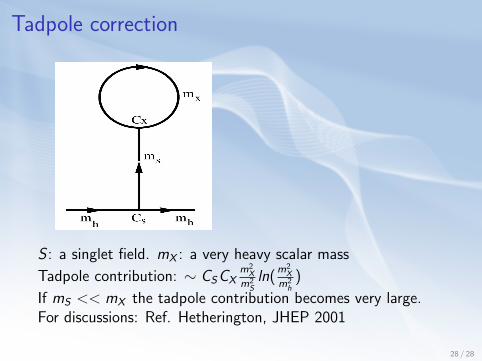
Tadpole correction

S : a singlet field. mX : a very heavy scalar mass

Tadpole contribution: ∼ CSCXm2

X

m2Sln(

m2X

m2h

)

If mS << mX the tadpole contribution becomes very large.For discussions: Ref. Hetherington, JHEP 2001

28 / 28

Hard SUSY breaking termsS. Martin, Phys. Rev D., 2000; Possible non-holomorphic hard SUSY breaking terms:

Type Term Naive Suppression Origin

φ4 FM2 ∼ mW

M1M2 [XΦ4]F

φ3φ∗ |F |2M4 ∼ m2

W

M21M4 [XX ∗Φ3Φ∗]D

φ2φ∗2 |F |2M4 ∼ m2

W

M21M4 [XX ∗Φ2Φ∗2]D

φψψ |F |2M4 ∼ m2

W

M21M4 [XX ∗ΦDαΦDαΦ]D

hard φ∗ψψ |F |2M4 ∼ m2

W

M21M4 [XX ∗Φ∗DαΦDαΦ]D

φψλ |F |2M4 ∼ m2

W

M21M4 [XX ∗ΦDαΦWα]D

φ∗ψλ |F |2M4 ∼ m2

W

M21M4 [XX ∗Φ∗DαΦWα]D

φλλ FM2 ∼ mW

M1M2 [XΦW αWα]F

φ∗λλ |F |2M4 ∼ m2

W

M21M4 [XX ∗Φ∗W αWα]D

28 / 28

Electroweak Fine-tuning Components

∆(µ) =4µ2

m2Z

(1 +

m2A + m2

Z

m2A

tan2 2β

),

∆(b) =

(1 +

m2A

m2Z

)tan2 2β,

∆(m2Hu

) =

∣∣∣∣∣ 1

2cos 2β +

m2A

m2Z

cos2β −

µ2

m2Z

∣∣∣∣∣×(

1−1

cos 2β+

m2A + m2

Z

m2A

tan2 2β

),

∆(m2Hu

) =

∣∣∣∣∣− 1

2cos 2β +

m2A

m2Z

sin2β −

µ2

m2Z

∣∣∣∣∣×∣∣∣∣∣1 +

1

cos 2β+

m2A + m2

Z

m2A

tan2 2β

∣∣∣∣∣ ,

∆Total =

√∑i

∆2pi, (1)

Ref. Perelstein, Spethmann: JHEP 2007, hep-ph/0702038

28 / 28

SM contributions: aSMµ

1 and 2-loop QED:

Weak contributions:

hadronic contributions:

28 / 28

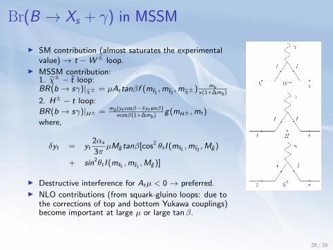
Br(B → Xs + γ) in MSSM

I SM contribution (almost saturates the experimentalvalue) → t −W± loop.

I MSSM contribution:1. χ± − t loop:BR(b → sγ)|χ± = µAttanβf (mt1 ,mt2 ,mχ±) mb

v(1+∆mb)

2. H± − t loop:

BR(b → sγ)|H± = mb(yt cosβ−δyt sinβ)vcosβ(1+∆mb)

g(mH± ,mt)

where,

δyt = yt2αs

3πµMg tanβ[cos2 θt I (msL ,mt2 ,Mg )

+ sin2θt I (msL ,mt1 ,Mg )]

I Destructive interference for Atµ < 0 → preferred.I NLO contributions (from squark-gluino loops: due to

the corrections of top and bottom Yukawa couplings)become important at large µ or large tanβ.

28 / 28

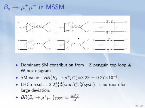
Bs → µ+µ− in MSSM

I Dominant SM contribution from : Z penguin top loop &W box diagram.

I SM value : BR(Bs → µ+µ−)=3.23 ± 0.27×10−9.

I LHCb result : 3.2+1.4−1.2(stat.)+0.5

−0.3(syst.)→ no room forlarge deviation.

I BR(Bs → µ+µ−)SUSY ∝ tan6βmA

4

28 / 28

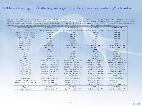
NH terms affecting or not affecting muon g-2 in two benchmark points where χ01 is bino-like

Table 1. Benchmark points for NHSSM. Masses are shown in GeV. Only the two NHSSM benchmark

points shown satisfy the phenomenological constraint of Higgs mass, dark matter relic density along with

direct detection cross section, muon anomaly, Br(B → Xs+γ) and Br(Bs → µ+µ−). The associated MSSM

points are only given for comparison and do not necessarily satisfy all the above constraints.

Parameters MSSM NHSSM MSSM NHSSM

m1,2,3 472, 1500, 1450 472, 1500, 1450 243, 250, 1450 243, 250, 1450

mQ3/mU3

/mD31000 1000 1000 1000

mQ2/mU2

/mD21000 1000 1000 1000

mQ1/mU1

/mD11000 1000 1000 1000

mL3/mE3

2236 2236 1000 1000

mL2/mE2

592 592 500 500

mL1/mE1

592 592 500 500

At, Ab, Aτ -1500, 0, 0 -1500, 0, 0 -1368.1, 0, 0 -1368.1, 0, 0

A′t, A

′µ, A

′τ 0, 0, 0 2234, 169, 0 0, 0, 0 3000, 200, 0

tanβ 10 10 40 40

µ 500 500 390.8 390.8

µ′ 0 -175 0 1655.5

mA 1000 1000 1000 1000

mg 1438.9 1439.1 1438.9 1438.9

mt1,mt2

894.4, 1151.2 865.5, 1154.9 907.8, 1137.5 903.4, 1141.4

mb1,mb2

1032.4, 1046.2 1026.3, 1045.1 1013.8, 1051.2 1017.7, 1056.5

mµL ,mνµ 596.4, 596.3 573.5, 595.9 502.0, 497.1 465.8, 496.3

mτ1 ,mντ 2237.1, 2238.5 2237.1, 2238.5 985.4, 997.2 988.5, 998.8

mχ±1,mχ±

2504.2, 1483.6 677.6, 1484.7 244.6, 421.0 262.3, 1255.2

mχ01,mχ0

2448.6, 509.0 464.0, 680.6 231.3, 249.9 240.9, 262.1

mχ03,mχ0

4522.6, 1483.5 683.2, 1484.7 400.7, 421.0 1253.3, 1253.7

mH± 1011.9 1005.8 955.7 1011.6

mH ,mh 1008.1, 121.4 984.8, 122.8 948.0, 122.4 990.2, 122.8

Br(B → Xs + γ) 3.00× 10−4 3.01× 10−4 2.01× 10−4 4.05× 10−4

Br(Bs → µ+µ−) 3.40× 10−9 3.45× 10−9 5.06× 10−9 1.65× 10−9

aµ 1.94× 10−10 22.3× 10−10 34.8× 10−10 35.8× 10−10

Ωχ01h2 0.035 0.095 0.0114 0.122

σSIχ01p

in pb 4.01× 10−9 3.47× 10−10 6.79× 10−9 3.15× 10−12

– 18 –

28 / 28

Electroweak fine-tuning and higgsino dark matter

∆Total vs mχ0

1for tan β = 10

MSSM (i.e. with µ′ = A′t = 0): Thin blue line andpartly green line in the middle. ∆Total is little above 400.

NHSSM: brown and magenta. Consistent region

satisfying a 3σ level of WMAP/PLANCK constraints are

shown. EWFT in NHSSM ranges from too high to too

low (∼ 50).

∆Total vs mχ0

1for tan β = 40

EWFT in NHSSM can be vanishingly small.−3 TeV < µ, µ′ < 3 TeV

−3 TeV < At,A′t < 3 TeV

EW fine-tuning differs from FT estimate in UV complete scenario like CMSSMwith NH terms. There, an FT expression would depend on NH parameters. TheFT related low scale parameters pi are no longer independent. NH+CMSSMstill has FT estimate dominantly controlled by µ2 (Ross et. al. 2016, 2017).

28 / 28