Embed Size (px)
Citation preview

Délivré par l’Université de Montpellier
Préparée au sein de l’école doctorale I2S - Information,Structures, Systèmes
Et de l’unité de recherche UMR 5149 - IMAG - InstitutMontpelliérain Alexander Grothendieck
Spécialité: Biostatistique
Présentée par Julien Stoehr
Méthodes d’inférencestatistique pour champs de
Gibbs
Soutenue le 29 octobre 2015 devant le jury composé de
Jean-Michel Marin Professeur Université de Montpellier DirecteurPierre Pudlo Professeur Université de Montpellier Co-directeurLionel Cucala Maître de Conférences Université de Montpellier Co-encadrantFlorence Forbes Directeur de recherche INRIA Grenoble Rhône-Alpes RapporteurHåvard Rue Professeur Norwegian University of Science Rapporteur
and TechnologyStéphanie Allassonnière Professeur chargée de cours École Polytechnique ExaminateurStéphane Robin Directeur de recherche INRA/AgroParisTech Président du
jury


Do the best you can until you know better.
Then, when you know better, do better.
— Maya Angelou
À la mémoire de ma grand-mère Marie-Madeleine, de mon grand-père Paul
et de mon amie Christiane.


Remerciements
S’il est un exercice qui s’avère tout aussi difficile que la rédaction de la thèse, c’est
bien l’écriture des remerciements. J’espère qu’au travers de ces lignes, je n’oublierai
de rendre hommage à aucune des personnes qui m’ont permis d’en être arrivé là.
Mes premiers remerciements vont tout naturellement à mes directeurs de thèse Jean-
Michel Marin, Pierre Pudlo et Lionel Cucala. Jean-Michel pour m’avoir initié à la
statistique bayésienne, pour avoir su laisser s’épanouir ma liberté de recherche tout
en me proposant un encadrement sans faille. Pour ton enthousiasme, pour ton soutien
constant aussi bien professionnel que personnel. Et enfin pour m’avoir fait découvrir
les beautés du vignoble languedocien. Pierre pour ta patience et ta disponibilité face à
l’étudiant chronophage et plein de questions que j’ai pu être. Pour ton investissement
hors norme qui m’a permis de gagner en maturité et de prendre du recul sur mes
travaux. Pour tes enseignements qui ont grandement contribué aux compétences que
j’ai développées au cours de cette thèse, soient elles mathématiques ou informatiques.
Lionel pour avoir été l’acteur de certaines tâches ingrates comme traiter à la main
des centaines de données. Pour ton œil de lynx infaillible qui traquait sans relâche
mes coquilles, parfois, plus que nombreuses. À tous les trois, pour la confiance que
vous m’avez accordée et pour tout ce que je ne peux simplement résumer en quelques
lignes, merci.
Je voudrais ensuite exprimer toute ma gratitude à Florence Forbes et Håvard Rue1
qui m’ont fait l’honneur de rapporter cette thèse avec beaucoup d’attention et de
rigueur malgré des emplois du temps chargés. L’intérêt que vous avez porté à mes
travaux, nos discussions et vos remarques sont pour moi le meilleur encouragement à
poursuivre dans le monde de la recherche.
À Stéphanie Allassonnière et Stéphane Robin pour avoir accepté de faire partie de ce
jury sans la moindre hésitation. J’aimerais, ici, également remercier Nathalie Peyrard.
1Jeg vil gjerne takke Håvard Rue, som gjorde meg den ære å gjennomgå denne avhandlingen på enoppmerksom og grundig måte til tross for en travel timeplan. Interessen du har vist for mitt arbeid, og idiskusjoner og tilbakemelding, er for meg den beste motivasjonen for å fortsette å forske.
i

Remerciements
Ce fut pour moi un immense privilège que Stéphanie et toi ayez suivi cette thèse
depuis ses débuts. Vos conseils lors des comités de suivi de thèse ont joué un rôle
primordial dans la réussite de ces travaux.
De façon plus générale, je souhaite remercier les membres de l’IMAG, et tout particu-
lièrement ceux de l’équipe EPS, pour votre accueil chaleureux. Un énorme merci à
Sophie Cazanave-Pin, Bernadette Lacan, Myriam Debus, Éric Hugounenq et Nathalie
Quintin. De par votre gentillesse, votre disponibilité, votre sympathie et votre aide pré-
cieuse en toute circonstance, vous êtes indiscutablement les super-héros du bâtiment
9. Une petite pensée pour Gemma Bellal qui a toujours un mot gentil. À Christian,
Catherine, Élodie, André, Fabien, Irène, Benjamin, Christophe, Gwladys, Jean-Noël,
Benoîte, Xavier, Ludovic, Cyrille, Baptiste, Mathieu, Pascal et Vanessa, que ce soit de
près ou de loin, vous avez contribué à faire de cette thèse une expérience enrichissante
et plaisante.
Une mention toute spéciale à Mathieu Ribatet pour tous nos échanges mathéma-
tiques, politiques ou sportifs autour d’une bonne bière (ou d’un plateau du restaurant
administratif... au choix). Ton amitié et ton soutien signifient beaucoup. Tu as accom-
pagné mes premiers pas d’enseignant et m’as fait profiter de tes compétences aussi
bien pédagogiques que scientifiques. Et si je devais te faire une dédicace particulière
dans cette thèse, ce serait le chapitre 2 auquel tu as grandement contribué sans être
officiellement impliqué.
Ali, je ne t’oublie pas. Tu me pardonneras les approximations orthographiques mais
que ce soit pour nos discussions sérieuses ou grivoiseries : choukran jazilan !
À celui qui en plus d’être mathématicien est également un SwingJammerz... Simon,
merci pour ton humour et ta simplicité.
I would like to thank Nial Friel. Your enthusiasm as I was just beginning my thesis has
been a source of motivation. Our collaboration is an integral part of this dissertation
and has driven us into interesting questions. I am looking forward working with you
in the future and developing all the project we already have.
Parmi tous mes professeurs, que je salue, je souhaite rendre un hommage tout par-
ticulier à deux d’entre eux. Nathalie Baumgarten, c’est avec toi que j’ai appris à lire.
Tu es le point de départ de ces longues années d’études et savoir qu’après tout ce
temps, tu continues de suivre mes pas d’écolier me fait chaud au cœur. Puis, cette
aventure montpelliéraine n’aurait pas eu lieu sans Benoît Cadre. Tu es celui par qui je
suis arrivé à la statistique. Tes conseils avisés et tes enseignements ont rendu tout cela
possible et je t’en suis extrêmement reconnaissant.
ii

Mes mots s’adressent maintenant aux doctorants actuels et passés pour les discus-
sions délirantes à base de petits poneys ou autres extravagances, et pour ces moments
de procrastination savamment dosés. Petit clin d’œil à mes co-bureaux : Benjamin qui
m’aura appris que les vraies mathématiques ne sont que des flèches à la craie blanche
sur un tableau noir... Et Joubine, que dire si ce n’est que tu resteras mon interlocuteur
privilégié concernant nordpresse.be ! Tu sais le succès que je te souhaite. Faire une
thèse, c’est aussi adopter une deuxième famille. Un énorme merci à mon grand-frère
de thèse Mohammed, ma petite sœur de thèse Coralie et mon petit demi-frère (ça
commence à devenir compliqué la filiation) Paul pour les moments de craquage
complet et tout le reste. Un seul regret : Momo il va définitivement falloir que tu
danses avec nous à la SFDS ! Merci à Mickaël Lallouche, partner in crime avec qui
j’ai pris énormément de plaisir à organiser le séminaire des doctorants. La liste est
encore longue et je n’ai pas de place ici pour raconter une anecdote sur tous mais vous
avez chacun eu une place particulière pendant cette thèse. Donc merci à Mathieu,
Angelina, Christophe, Yousri (aka Yousri the King), Étienne, Myriam, Jérémie, Gautier,
Nahla, Théo, Quentin, Boushra, Nejib, Romain, Wallid, Amina, Emmanuelle, Clau-
dia, Alexandre, Hanen, Guillaume, David, Mike, Antoine, Alaaeddine, Anis, Jocelyn,
Rebecca, Anthony, Wenran, Samuel, Francesco, Christian, Tutu, Elsa.
À cette longue liste je souhaite ajouter toutes les personnes avec qui j’ai pu discuter lors
de congrès ou de séminaires. Chaque échange a été l’occasion de faire avancer mes
travaux, de parfaire ou d’enrichir ma culture scientifique. Un merci tout particulier
à Christian Robert pour ses critiques toujours bénéfiques, à Benjamin Guedj pour
toutes ses recommandations, et enfin à Florian Maire pour son aide à Dublin.
L’achèvement d’une thèse passe par le subtil dosage entre ambiance studieuse et sas
de décompression. Tout ce travail n’aurait donc simplement pas été possible sans
ma famille et mes amis. À commencer par la dream team qui a répondu présente à
chacune de mes convocations loufoques. Je ne compte plus les matchs joués ni les
buts marqués, mais Arnold (tu peux le dire maintenant que tu as 28 ans...), Romain,
Rémi, Fabien, Isaie, Will, Ju, Tom, Max et Nico : une chose est sûre, ce qu’on a toujours
réussi ce sont les troisièmes mi-temps.
Je me dois ensuite de remercier ceux qui ont partagé une bonne partie de ma vie
pendant cette thèse : les SwingJammerz. À Oliv, Ben dit Scapino, JB, Tat pour m’avoir
accueilli et inspiré au quotidien. À Isaie et Claire pour votre confiance et votre soutien
permanent. À Sand, Mimi, Chacha, et Christelle, pour avoir été des partenaires et des
amies exceptionnelles. À Richard, Mélody, Billy, Annabelle et Sixte pour m’avoir fait
découvrir les joies de la team dont je ne peux citer le nom ici ! À Anne pour m’avoir
transmis le virus irlandais. À Karine pour ton optimisme indéfectible. À tous, un
iii

Remerciements
énorme merci pour les centaines de danses et les bons moments que nous avons
partagés. À mes chouchous qui m’ont suivi et supporté en cours de danse comme
en dehors, les Joséphine (Myriam, Émilie, Sally), David, Franck, Clara, Jean-Marie,
Marion & Marion, Jérémy et Fabien : keep on swinging !
À tous mes amis de la scène qui ont impulsé mes travaux sur le parquet comme
en dehors : Paulo, JP, Marlène, Irène, Lionel, Audrey, Aurélien, Rija, Peter, Marielle,
Béné, Paulopaul, Liliane, Henry, Margaux, Alexis, Aline, Niko, Audrey, Patrick, Patricia,
Jean-Marc, Céline, Séb, Anne-Laure et tout ceux que j’oublie de citer. À Charlie mon
camarade de voyage. À Flo une amie, une confidente, une révélatrice de créativité. À
Line, Gildas, Maxence et Corentin, l’alliance parfaite de l’Alsace et de la Bretagne. À
Thomas, Annie, Max, Dax et Sarah pour m’avoir aidé à me dépasser, à persévérer ! À
Will et Maéva pour avoir été là dans les bons comme dans les mauvais moments, pour
me rappeler au quotidien que tout ou presque est possible à force de travail. Je vous
embrasse !
À cette liste quasi exhaustive, il faut ajouter celles et ceux qui ont su faire de Montpellier
un foyer chaleureux où il fait bon vivre. À mes collocs Mathieu, Maïwenn et Jérémie qui
ont fait en sorte que la rédaction de ce manuscrit se passe dans des conditions idéales.
Votre amitié a été plus que bénéfique et appréciable dans les derniers kilomètres de
ce marathon qu’est la thèse. J’ai également une pensée pour mes collocs des premiers
jours Alice et Peter. De L.A. à Montpellier vous avez tous deux apporté beaucoup de
soleil dans ma vie de doctorant. À Katy, une muse inattendue qui a su faire avancer
ma réflexion. À Sally et Sylvia pour avoir donné une toute autre dimension aux soirées
Love Boat. À Hélian qui me laisse pantois d’admiration. À Julien mon bricoleur
préféré, tu as été un compagnon de galère et le complice parfait en toute circonstance.
À Vincent, mein elsässicher Freund, le seul ici à connaître la véritable grandeur de
notre région... Et surtout le seul à savoir que le Sundgau n’est pas une région d’Afrique.
À Pacchus mon président de cœur plein de philosophie. À Jean et Maud parce qu’on
pourrait presque tout résumer à une soirée quizz épique. À Leslie, Ev’ Ma, Val et
Pauline, pour les bouffées d’air frais. À Pierre Malaka pour l’analyse anthropologique
et psychologique des microcosmes ambiants ou tout simplement pour être toi. À
Carine un amour de volleyeuse pour ton oreille attentive et ta joie de vivre.
Pour terminer, il me reste à rendre hommage à ceux qui sont les plus chers à mon cœur.
À ma marraine et René, mon parrain et Léa, Fabienne, Didier, Lulu, Nico, Alex, Élise,
Patrice, Marie-Christine, Christian et Natacha pour avoir été présents, pour m’avoir
encouragé d’aussi loin que je m’en souvienne. À la Bes Léa, au Bof Guillaume et à vos
parents pour être une belle famille au top niveau. À Bernard, tu as été pour moi un
peu comme un grand-père... Avec Christiane vous n’avez manqué aucune des étapes
iv

importantes qui m’ont conduit ici. Cela a toujours compté énormément pour moi et
mon seul regret aujourd’hui est qu’elle ne soit pas avec nous pour partager ce moment.
À Mamie, même dépassée par mon parcours universitaire tu t’es toujours souciée
de mon avenir. Le petit garçon qui courait dans les prés et les forêts d’Horodberg
a bien grandi et j’aurais aimé que Papi voit ce que l’homme que je suis devenu a
réussi à accomplir. À Mémé qui malgré la distance m’a toujours porté, m’a toujours
donné la motivation pour faire de mon mieux. Je sais que tu continueras à veiller
sur moi de là où tu es. À Noémie, Sébastien et Baptiste, j’espère remplir mon rôle de
grand-frère aussi bien que possible. Il n’existe pas qu’un seul exemple de réussite et
vous en êtes l’exemple parfait. J’espère vous apporter au quotidien autant que ce que
chacun d’entre vous m’apporte. À Maman et Papa vous m’avez enseigné le respect,
l’humilité et l’amour du travail bien fait. Même dans les moments de doutes, vous
n’avez jamais cessé de croire en moi. J’ai toujours eu à cœur d’exceller pour être à la
hauteur des sacrifices que, sans hésiter, vous avez faits pour nous, pour être digne de
l’amour et du soutien que vous nous avez toujours témoignés. La plus belle réussite,
le plus beau cadeau, c’est de vous savoir fiers et, en dépit de tous les aléas de la vie,
inconditionnellement présents. À tous, simplement et sincèrement merci !
v


Contents
Remerciements i
List of figures ix
List of tables xi
Introduction 1
1 Statistical analysis issues for Markov random fields 9
1.1 Markov random field and Gibbs distribution . . . . . . . . . . . . . . . . 9
1.1.1 Gibbs-Markov equivalence . . . . . . . . . . . . . . . . . . . . . . 9
1.1.2 Autologistic model and related distributions . . . . . . . . . . . . 12
1.1.3 Phase transition . . . . . . . . . . . . . . . . . . . . . . . . . . . . . 15
1.1.4 Hidden Gibbs random field . . . . . . . . . . . . . . . . . . . . . . 17
1.2 How to simulate a Markov random field . . . . . . . . . . . . . . . . . . . 18
1.2.1 Gibbs sampler . . . . . . . . . . . . . . . . . . . . . . . . . . . . . . 19
1.2.2 Auxiliary variables and Swendsen-Wang algorithm . . . . . . . . 20
1.3 Recursive algorithm for discrete Markov random field . . . . . . . . . . 22
1.4 Parameter inference: maximum pseudolikelihood estimator . . . . . . 26
1.5 Parameter inference: computation of the maximum likelihood . . . . . 28
1.5.1 Monte Carlo maximum likelihood estimator . . . . . . . . . . . . 29
1.5.2 Expectation-Maximization algorithm . . . . . . . . . . . . . . . . 30
1.7 Parameter inference: computation of posterior distributions . . . . . . 36
1.7.1 The single auxiliary variable method . . . . . . . . . . . . . . . . 37
1.7.2 The exchange algorithm . . . . . . . . . . . . . . . . . . . . . . . . 39
1.8 Model selection . . . . . . . . . . . . . . . . . . . . . . . . . . . . . . . . . 41
1.8.1 Bayesian model choice . . . . . . . . . . . . . . . . . . . . . . . . . 41
1.8.2 ABC model choice approximation . . . . . . . . . . . . . . . . . . 42
1.8.3 Bayesian Information Criterion approximations . . . . . . . . . . 46
2 Adjustment of posterior parameter distribution approximations 53
2.1 Bayesian inference using composite likelihoods . . . . . . . . . . . . . . 53
vii

Contents
2.1.1 Composite likelihood . . . . . . . . . . . . . . . . . . . . . . . . . 53
2.1.2 Conditional composite posterior distribution . . . . . . . . . . . 57
2.1.3 Estimation algorithm of the Maximum a posteriori . . . . . . . . 58
2.1.4 On the asymptotic theory for composite likelihood inference . . 61
2.2 Conditional composite likelihood adjustments . . . . . . . . . . . . . . 63
2.2.1 Magnitude adjustment . . . . . . . . . . . . . . . . . . . . . . . . . 63
2.2.2 Curvature adjustment . . . . . . . . . . . . . . . . . . . . . . . . . 64
2.2.3 Mode adjustment . . . . . . . . . . . . . . . . . . . . . . . . . . . . 65
2.3 Examples . . . . . . . . . . . . . . . . . . . . . . . . . . . . . . . . . . . . . 67
3 ABC model choice for hidden Gibbs random fields 733.1 Local error rates and adaptive ABC model choice . . . . . . . . . . . . . 74
3.1.1 Background on Approximate Bayesian computation for model
choice . . . . . . . . . . . . . . . . . . . . . . . . . . . . . . . . . . 74
3.1.2 Local error rates . . . . . . . . . . . . . . . . . . . . . . . . . . . . . 78
3.3.1 Estimation algorithm of the local error rates . . . . . . . . . . . . 81
3.3.2 Adaptive ABC . . . . . . . . . . . . . . . . . . . . . . . . . . . . . . 82
3.4 Hidden random fields . . . . . . . . . . . . . . . . . . . . . . . . . . . . . 84
3.4.1 Hidden Potts model . . . . . . . . . . . . . . . . . . . . . . . . . . 84
3.4.2 Geometric summary statistics . . . . . . . . . . . . . . . . . . . . 86
3.4.3 Numerical results . . . . . . . . . . . . . . . . . . . . . . . . . . . . 89
4 Model choice criteria for hidden Gibbs random field 954.1 Block Likelihood Information Criterion . . . . . . . . . . . . . . . . . . . 96
4.1.1 Background on Bayesian Information Criterion . . . . . . . . . . 96
4.2.1 Gibbs distribution approximations . . . . . . . . . . . . . . . . . 99
4.2.2 Related model choice criteria . . . . . . . . . . . . . . . . . . . . . 102
4.3 Comparison of BIC approximations . . . . . . . . . . . . . . . . . . . . . 102
4.3.1 Hidden Potts models . . . . . . . . . . . . . . . . . . . . . . . . . . 103
4.3.2 First experiment: selection of the number of colors . . . . . . . . 104
4.3.3 Second experiment: selection of the dependency structure . . . 105
4.3.4 Third experiment: BLIC versus ABC . . . . . . . . . . . . . . . . . 107
Conclusion 109
Bibliography 113
viii

List of Figures
1.1 First and second order neighborhood graphs G with corresponding cliques. (a)
The four closest neighbors graph G4. Neighbors of the vertex in black are repre-
sented by vertices in gray. (b) The eight closest neighbors graph G8. Neighbors
of the vertex in black are represented by vertices in gray. (c) Cliques of graph
G4. (d) Cliques of graph G8. . . . . . . . . . . . . . . . . . . . . . . . . . . . . 10
1.2 Realization of a 2-states Potts model for various interaction parameter β on a
100×100 lattice with a first-order neighborhood (first row) or a second-order
neighborhood (second row). . . . . . . . . . . . . . . . . . . . . . . . . . . . 15
1.3 Phase transition for a 2-states Potts model with respect to the first order and
second order 100×100 regular square lattices. (a) Average proportion of homo-
geneous pairs of neighbors. (b) Variance of the number of homogeneous pairs
of neighbors. . . . . . . . . . . . . . . . . . . . . . . . . . . . . . . . . . . . 17
1.4 Auxiliary variables and subgraph illustrations for the Swendsen-Wang algo-
rithm. (a) Example of auxiliary variables Ui j for a 2-states Potts model configu-
ration on the first order square lattice. (b) Subgraph Γ(G4,x) of the first order
lattice G4 induced by the auxiliary variables Ui j . . . . . . . . . . . . . . . . . 21
2.1 Posterior parameter distribution (plain), non-calibrated composite posterior
distribution (dashed) and composite posterior distribution (green) with a uni-
form prior for a realization of the Ising model on a 16×16 lattice near the phase
transition. The conditional composite likelihood is computed for an exhaustive
set of 4×4 blocks. . . . . . . . . . . . . . . . . . . . . . . . . . . . . . . . . . 58
2.2 First experiment results. (a) Posterior parameter distribution (plain), non-
calibrated composite posterior parameter distribution (dashed) and composite
posterior distribution (green) of a first-order Ising model. (b) Boxplot displaying
the ratio of the variance of the composite posterior parameter by the variance
of the posterior parameter for 100 realisations of a first-order Ising model. . . 68
ix

List of Figures
2.3 Second experiment results. (a) Posterior parameter distribution (grey) and
non-calibrated composite posterior parameter distribution (pink) for a first-
order anisotropic Ising model. (b) Posterior parameter distribution (grey) and
composite posterior parameter distribution (green) with mode and magnitude
adjustments (w = w (2)). (c) Boxplots displaying 1p2‖VarCL(θ)Var−1(θ)‖F for 100
realisations of an anisotropic first-order Ising model. . . . . . . . . . . . . . . 70
2.4 Third experiment results. (a) Posterior parameter distribution (grey) and non-
calibrated composite posterior parameter distribution (pink) for a first-order
autologistic model. (b) Posterior parameter distribution (grey) and composite
posterior parameter distribution (green) with mode and curvature adjustments
(W = W (4)). (c) Boxplots displaying 1p2‖VarCL(ψ)Var−1(ψ)‖F for 100 realisa-
tions of a first-order autologistic model. . . . . . . . . . . . . . . . . . . . . . 72
3.1 The induced graph Γ(G4,y
)and Γ
(G8,y
)on a given bicolor image y of size
5× 5. The six summary statistics on y are thus R(G4,y
) = 22, T(G4,y
) = 7,
U(G4,y
)= 12, R(G8,y
)= 39, T(G8,y
)= 4 and U(G8,y
)= 16 . . . . . . . . . . . 87
3.2 First experiment results. (a) Prior error rates (vertical axis) of ABC with respect
to the number of nearest neighbors (horizontal axis) trained on a reference
table of size 100,000 (solid lines) or 50,000 (dashed lines), based on the 2D,
4D and 6D summary statistics. (b) Prior error rates of ABC based on the 2D
summary statistic compared with 4D and 6D summary statistics including
additional ancillary statistics. (c) Evaluation of the local error on a 2D surface. 90
3.3 Third experiment results. (a) Prior error rates (vertical axis) of ABC with re-
spect to the number of nearest neighbors (horizontal axis) trained on a refer-
ence table of size 100,000 (solid lines) or 50,000 (dashed lines), based on the
2D, 4D and 6D summary statistics. (b) Prior error rates of ABC based on the
2D summary statistics compared with 4D and 6D summary statistics including
additional ancillary statistics. (c) Evaluation of the local error on a 2D surface. 93
4.1 First experiment results. (a) BICMF-like, BICGBF and BLICMF-like2×2 values for one
realization of a first order hidden Potts model HPM(G ,θ,4). (b) Difference
between BLICMF-like2×2 values for 100 realization of a first order hidden Potts
model HPM(G4,θ,4) as K is increasing. (c) Difference between BLIC2×2 values
for 100 realization of a first order hidden Potts model HPM(G4,θ,4) as K is
increasing . . . . . . . . . . . . . . . . . . . . . . . . . . . . . . . . . . . . . 106
x

List of Tables
1.1 Interaction parametrisation for a homogeneous Gibbs random field in isotropic
and anisotropic cases. The table gives values of the parameter βi j correspond-
ing to the orientation of the edge (i , j ). . . . . . . . . . . . . . . . . . . . . . 13
1.2 Illustration of the curse of dimensionality for various dimension d and sample
sizes N . . . . . . . . . . . . . . . . . . . . . . . . . . . . . . . . . . . . . . . 44
2.1 Weight options for a magnitude adjustment in presence of anisotropy or poten-
tial on singletons (ψ ∈Rd ) . . . . . . . . . . . . . . . . . . . . . . . . . . . . 64
2.2 Evaluation of the relative mean square error (RMSE) and the expected KL-
divergence (EKLD) between the approximated posterior and true posterior
distributions for 100 simulations of a first-order Ising model in the first experi-
ment. . . . . . . . . . . . . . . . . . . . . . . . . . . . . . . . . . . . . . . . 69
2.3 Evaluation of the relative mean square error (RMSE) the expected KL-divergence
(EKLD) between the composite posterior distribution and true posterior distri-
bution for 100 simulations of an anisotropic first-order Ising model. . . . . . 71
2.4 Evaluation of the relative mean square error (RMSE) for 100 simulations of a
first-order autologistic model. . . . . . . . . . . . . . . . . . . . . . . . . . . 71
3.1 Evaluation of the prior error rate on a test reference table of size 30,000 in the
first experiment. . . . . . . . . . . . . . . . . . . . . . . . . . . . . . . . . . 91
3.2 Evaluation of the prior error rate on a test reference table of size 20,000 in the
second experiment. . . . . . . . . . . . . . . . . . . . . . . . . . . . . . . . . 92
3.3 Evaluation of the prior error rate on a test reference table of size 30,000 in the
third experiment. . . . . . . . . . . . . . . . . . . . . . . . . . . . . . . . . . 92
4.1 Selected K in the first experiment for 100 realizations from HPM(G4,θ,4) and
100 realizations from HPM(G8,θ,4) using Pseudolikelihood Information Cri-
terion (PLIC), mean field-like approximations (BICMF-like, BICGBF) and Block
Likelihood Information Criterion (BLIC) for various sizes of blocks and border
conditions. . . . . . . . . . . . . . . . . . . . . . . . . . . . . . . . . . . . . 105
xi

List of Tables
4.2 Selected G in the second experiment for 100 realizations from HPM(G4,θ,4)
and 100 realizations from HPM(G8,θ,4) using Pseudolikelihood Information
Criterion (PLIC), mean field-like approximations (BICMF-like, BICGBF) and Block
Likelihood Information Criterion (BLIC) for various sizes of blocks and border
conditions. . . . . . . . . . . . . . . . . . . . . . . . . . . . . . . . . . . . . 107
4.3 Evaluation of the prior error rate of ABC procedures and of the error rate for
the model choice criterion in the third experiment. . . . . . . . . . . . . . . . 108
xii

Introduction
The problem of developing satisfactory methodology for the analysis of spatial data
has been of a constant interest for more than half a century now. Constructing a
joint probability distribution to describe the global properties of data is somewhat
complicated but the difficulty can be bypassed by specifying the local characteristics
via conditional probability instead. This proposition has become feasible with the
introduction of Markov random fields (or Gibbs distribution) as a family of flexible
parametric models for spatial data (the Hammersley-Clifford theorem, Besag, 1974).
Markov random fields are spatial processes related to lattice structure, the conditional
probability at each nodes of the lattice being dependent only upon its neighbors,
that is useful in a wide range of applications. In particular, hidden Markov random
fields offer an appropriate representation for practical settings where the true state is
unknown. The general framework can be described as an observed data y which is a
noisy or incomplete version of an unobserved discrete latent process x.
Gibbs random fields originally come from physics (see for example, Lanford and
Ruelle, 1969) but have been useful in many other modelling areas. Indeed, they
have appeared as convenient statistical model to analyse different types of spatially
correlated data. Notable examples are the autologistic model (Besag, 1974) and its
extension the Potts model. Shaped by the development of Geman and Geman (1984)
and Besag (1986), these models have enjoyed great success in image analysis (e.g.,
Stanford and Raftery, 2002, Celeux et al., 2003, Forbes and Peyrard, 2003, Hurn et al.,
2003, Alfò et al., 2008, Moores et al., 2014) but also in other applications including
disease mapping (e.g., Green and Richardson, 2002) and genetic analysis (François
et al., 2006, Friel et al., 2009) to name a few. The exponential random graph model
or p∗ model (Wasserman and Pattison, 1996) is another prominent example (Frank
and Strauss, 1986) and arguably the most popular statistical model for social network
analysis (e.g., Robins et al., 2007).
Despite its popularity, the Gibbs distribution suffers from a considerable compu-
tational curse since its normalizing constant is of combinatorial complexity and
1

Introduction
generally can not be evaluated with standard analytical or numerical methods. This
forms a central issue in Bayesian inference as the computation of the likelihood is
an integral part of the procedure. Many deterministic or stochastic approximations
have been proposed for circumventing this difficulty and developing methods that are
computationally efficient and accurate is still an area of active research. Mention first
of all likelihood approximations involving a product of easily normalised distributions:
the pseudolikelihood (Besag, 1974, 1975), mean field approximations (e.g., Celeux
et al., 2003, Forbes and Peyrard, 2003), the reduced dependence approximation (Friel
et al., 2009) and composite likelihoods (e.g., Okabayashi et al., 2011, Friel, 2012). On
the other hand Monte Carlo approaches have played a major role to estimate the
intractable likelihood such as the maximum likelihood estimator of Geyer and Thomp-
son (1992) or the path sampling approach of Gelman and Meng (1998). More recently
Møller et al. (2006) present an auxiliary variable scheme that tackles this problem
by cancelling out the estimation of the normalizing constant, a work then further
developed by Murray et al. (2006) in their exchange algorithm. Another opportunity
is the approximate Bayesian computation (Pritchard et al., 1999) which provides a
Monte Carlo approximation of the targeted distribution. These manifold techniques
are reviewed among others and compared by Everitt (2012). Their main drawback is
the computing time involved that can be considerable. Alternatively McGrory et al.
(2009) construct a variational Bayes scheme with more efficient computing time to
analyse hidden Potts model.
The present work cares about the problem of carrying out Bayesian inference for
Markov random field. When dealing with hidden random fields, the focus is solely on
hidden data represented by Ising or Potts models. Both are widely used examples and
representative of the general level of difficulty. Aims may be to infer on parameters of
the model or on the latent state x.
Adjustment of posterior parameter distribution approxi-
mations
The first part of the present dissertation proposes to adjust substitute to the intractable
posterior parameter distribution. One of the earliest approaches to overcome the trou-
blesome constant is the pseudolikelihood method (Besag, 1974, 1975) which replaces
the likelihood function by the product of tractable full-conditional distributions of
all nodes. However the pseudolikelihood is not a genuine probability distribution
and leads to unreliable estimate of parameters (e.g., Geyer, 1991, Friel and Pettitt,
2004, Cucala et al., 2009). Despite this drawback, the pseudolikelihood has been used,
2

if only for its simplicity of calculation, in a wide range of applications, especially in
hidden Markov settings following the work of Besag et al. (1991) like in Heikkinen
and Hogmander (1994), Rydén and Titterington (1998). A natural generalization to
consider is the composite likelihood (Lindsay, 1988) which refines pseudolikelihood
by considering products of larger collections of variables. Composite likelihood has
been made popular in a context where marginal distributions can be computed (e.g.,
Varin et al., 2011, and references therein). Spatial lattice processes differ from that
class of models in the sense that dependence structure makes impossible the calcula-
tion of marginal probabilities and require the application of conditional composite
likelihood instead.
The purpose of this work is to use such composite likelihood methods for Bayesian
inference on observed Markov random fields. Currently, there is very little literature
on that possibility, although Pauli et al. (2011) and Ribatet et al. (2012) present a
discussion on the use of marginal composite likelihoods in a Bayesian setting. As
the neighbors relationship for Potts model is too complicated, the interest is solely
on conditional composite likelihood. Friel (2012) had a similar focus and studied
how the size of the collections of variables influences the resulting approximate
posterior distribution. His work follows a study conducted by Okabayashi et al. (2011)
although from a likelihood inference perspective. As in this dissertation, both consider
composite likelihood consisting in a product of joint distributions of collections of
neighbouring variables, namely blocks (or windows) of the lattice. The peculiarity
of Friel (2012) lies in the exact computation of conditional composite likelihood for
moderately large blocks using the recursive algorithm of Reeves and Pettitt (2004) for
general factorizable models, like Potts model, a method generalizing a result known for
hidden Markov models (Zucchini and Guttorp, 1991, Scott, 2002). The latter recursion
is a tempting alternative to stochastic approximations such as the path sampling
approach (Gelman and Meng, 1998). In the same way of Friel et al. (2009), we plug
it in a procedure that leads to reliable estimates based on exact calculation on small
lattices.
The main contribution of this work is the adjustment of posterior distributions result-
ing from using a misspecified likelihood function, referred to as composite posterior
distribution. Indeed, Friel (2012) is interested in the impact of the size of the blocks,
but he does not take advantage of the possibly weighting of blocks, even though he
observes that non-calibrated composite likelihood leads to overly precise posterior
parameters due to a substantial lower variability of the surrogate distribution. The
adjustment of composite likelihoods has long-standing antecedents in the frequentist
paradigm (e.g., Geys et al., 2001, Chandler and Bate, 2007), the primary goal being
to recover a chi-squared asymptotic null distribution. Our approach differs from the
3

Introduction
latter in the sense we make a shift from asymptotical behaviour of the composite
likelihood to local matching conditions about the posterior distribution. A key feature
to our proposal is the closed form of the gradient and of the Hessian matrix of the
log-posterior. Consequently it is possible to implement optimization algorithms that
allows to adjust the mode and the curvature at the mode of the composite posterior
distribution. Note that similar approach has been proposed in the context of Gaussian
Markov random fields (Rue et al., 2009).
Here we focus especially on how to formulate conditional composite likelihoods for
application to the autologistic model with possible anisotropy on the lattice. We
present numerical result for lattices small enough so that the true posterior distribu-
tion can be computed using the recursion of Reeves and Pettitt (2004) and serves as
a ground truth against which to compare the adjusted and non-adjusted composite
posterior distributions. The calibration is achieved for composite likelihoods that use
exhaustively all the blocks of the image, a challenging situation since there is a multi-
ple use of the data. The good results make this procedure an option worth exploring
for more complex settings such as hidden data or exponential random graph.
Approximate Bayesian computation model choice between
hidden Markov random fields
The second part of the current work aims at addressing the problem of selecting a
dependency structure for a hidden Markov random field in the Bayesian paradigm
and explores the opportunity of approximate Bayesian computation (e.g., Tavaré
et al., 1997, Pritchard et al., 1999, Marin et al., 2012, Baragatti and Pudlo, 2014). Up to
our knowledge, this important question has not yet been addressed in the Bayesian
literature. Alternatively we could have tried to set up a reversible jump Markov chain
Monte Carlo, but follows an important work for the statistician to adapt the general
scheme, as shown by Caimo and Friel (2011, 2013) in the context of exponential
random graph models where the observed data is a graph.
The Bayesian approach to model selection is based on posterior model probabili-
ties. When dealing with models whose likelihood cannot be computed analytically,
Bayesian model choice becomes challenging since the evidence of each model writes
as the integral of the likelihood over the prior distribution of the model parameter. To
answer the question of model choice, different opportunities have been tackled in
the literature but approximate Bayesian computation (ABC) method has appeared
as one of the most satisfactory approach to deal with intractable likelihood . ABC is
a simulation based approach that compares the observed data yobs with numerous
4

simulations y through summary statistics S(y) in order to supply a Monte Carlo ap-
proximation of the posterior probabilities of each model. The choice of such summary
statistics presents major difficulties that have been especially highlighted for model
choice (Robert et al., 2011, Didelot et al., 2011). Beyond the seldom situations where
sufficient statistics exist and are explicitly known (Gibbs random fields are surprising
examples, see Grelaud et al., 2009), Marin et al. (2014) provide conditions which en-
sure the consistency of ABC model choice. The present work has thus to answer the
absence of available sufficient statistics for hidden Potts fields as well as the difficulty
(if not the impossibility) to check the above theoretical conditions in practice.
Recent articles have proposed automatic schemes to construct theses statistics (rarely
from scratch but based on a large set of candidates) for Bayesian parameter inference
and are meticulously reviewed by Blum et al. (2013) who compare their performances
in concrete examples. But very few has been accomplished in the context of ABC
model choice apart from the work of Prangle et al. (2014). The statistics S(y) re-
constructed by Prangle et al. (2014) have good theoretical properties (those are the
posterior probabilities of the models in competition) but are poorly approximated
with a pilot ABC run (Robert et al., 2011), which is also time consuming.
ABC model choice is here presented as a k-nearest neighbor classifier, and we define a
local error rate which is the first contribution of the current work. We also provide an
adaptive ABC algorithm based on the local error to select automatically the dimension
of the summary statistics. The second contribution is the introduction of a general and
intuitive approach to produce geometric summary statistics for hidden Potts model.
This part of the dissertation concludes with numerical results in that framework.
Especially, we show with our approach that the number of simulation required by
ABC can be significantly cut down reducing at the same time the computational cost
whilst preserving performances.
Approximate model choice criterion: the Block Likelihood
Information Criterion
The last contribution considers model choice criterion for selecting the probabilis-
tic model that best accounts for the observation. This work is motivated by a more
general issue than the choice of an underlying graph for which we explore the oppor-
tunity of the Bayesian Information Criterion (BIC) (Schwarz, 1978) to overcome the
computational burden of ABC algorithms. Model choice is a problem of probabilistic
model comparison. The standard approach to compare one model against another
is based on the Bayes factor (Kass and Raftery, 1995) that involves the ratio of the
5

Introduction
evidence of each model. As already mentioned the evidence can not be computed
with standard procedure due to a high-dimensional integral. Various approximations
have been proposed but a commonly used one, if only for its simplicity, is BIC that is
an asymptotic estimate of the evidence based on the Laplace method. The criterion
is is a simple penalized function of the maximized log-likelihood. In this last part of
the dissertation, we provide an approximation of BIC able to infer both the number of
latent states and the dependency structure of a discrete hidden Markov random field.
The question of inferring the number of latent states has been recently tackled by
Cucala and Marin (2013) with an Integrated Completed Likelihood criterion(Biernacki
et al., 2000) but their complex algorithm cannot be extended easily to choose the
dependency structure.
In the context of Markov random fields, the difficulty comes from the maximized
log-likelihood part in BIC. Indeed, it involves the Gibbs distribution whose exact
computation is generally not feasible. For observed random field solutions proposed
to circumvent the problem are based for example on penalized pseudolikelihood
(Ji and Seymour, 1996) and MCMC approximations of BIC (Seymour and Ji, 1996).
When the random field is hidden little has been done before the work of Stanford and
Raftery (2002) and Forbes and Peyrard (2003). Both are interested in the question
of inferring the number of latent states and propose approximations that consist in
replacing the true likelihood with a product distribution on system of independent
variables to make the computation tractable. Stanford and Raftery (2002) handle the
burdensome likelihood with the pseudolikelihood of Qian and Titterington (1991) to
yield the so called Pseudo-Likelihood Information Criterion (PLIC). The latter appears
to be encompassed in the class of mean field-like approximations of BIC proposed by
Forbes and Peyrard (2003).
The proposal of Forbes and Peyrard (2003) derives from variational method that
provides a way to approximate the distribution through the introduction of a simpler
function that minimizes the Kullback-Leibler divergence between surrogate functions
and the Gibbs distribution. The divergence is minimized over the set of probability
distributions that factorize in a product on a set of single independent variables. Our
main contribution is to show that larger collections of variables, namely blocks of the
lattice, can be considered by taking advantage of the exact recursion of Reeves and
Pettitt (2004) and leads to an efficient criterion : the Block Likelihood Information
Criterion (BLIC). In particular, we will show that a reasonable approximation of the
Gibbs distribution is a product of Gibbs distributions on each independent block. To
assess the performances of the novel criterion, it is compared to the previous ones on
simulated data sets. Overall the criterion shows good results with notable benefits for
the estimation of the number of latent states. We fill in our study with a comparison
6

between BLIC and our second contribution related to ABC.
Overview
Chapter 1 is a reminder on Markov random fields introducing the notation and the
model of interest. It is an opportunity to present a brief state of the art related to
the inference issues tackled in this dissertation. Each chapter is then dedicated to
my own contributions to the analysis of Markov random fields. Chapter 2 presents
a correction of composite likelihoods to approximate the posterior distribution of
model parameter when the Markov random field is observed. My proposal is based
on the modification of the mode and the curvature at the mode of an approximated
posterior distribution resulting from a misspecified function to recover the true poste-
rior parameter distribution. This solution is appealing since its computational cost
is much lower than the Monte Carlo approaches such as the exchange algorithm
or the approximate Bayesian computation. The performances of the correction are
illustrated through simulated realizations of isotropic and anisotropic Ising models.
Both Chapters 3 and 4 are devoted to the question of model choice between hidden
Gibbs random fields. Throughout this dissertation, we tackle two model choice is-
sues: choosing the dependency structure and/or the number of latent states. My first
contribution developed in Chapter 3 concerns the approximate Bayesian computa-
tion methodology. The major difficulties addressed in Chapter 3 is the absence of
relevant summary statistics to choose a latent neighborhood structure. Chapter 3
first introduces a local error rate. The latter aims at evaluating the quality of a set
of summary statistics in the absence of the sufficiency property. Then I introduce
intuitive geometric summary statistics that leads to an efficient ABC model choice
procedure. Some numerical results are given to show the accuracy of the algorithm.
Chapter 4 extends the scope to a more general problem: the inference of the number
of latent states and the dependency structure. The main contribution of that part is to
replace the intractable likelihood with a product distribution on independent blocks
of a regular grid of nodes. Contrary to the substitute pixel by pixel proposed in the
literature, I suggest to include more spatial information by taking advantage of the
opportunity to make exact computation on small enough lattices. This leads a novel
approximation of BIC which is compared to PLIC (Stanford and Raftery, 2002) and
BIC approximations proposed by Forbes and Peyrard (2003) through simulated data.
Conclusions and further discussions are given at the end of the dissertation.
7


1 Statistical analysis issues for Markovrandom fields
Markov random fields have been used in many practical settings, surged by the de-
velopment in the statistical community since the 1970’s. Interests in these models
is not so much about Markov laws that may govern data but rather the flexible and
stabilizing properties they offer in modelling. The chapter presents a synopsis on
the existence of Markov random fields with some specific examples in Section 1.1.
The difficulties inherent to the analysis of the stochastic model are especially pointed
out. As befits a first chapter, a brief state of the art concerning parameter inference
(Section 1.4 and Section 1.5) and model selection (Section 1.8) is presented.
1.1 Markov random field and Gibbs distribution
1.1.1 Gibbs-Markov equivalence
A random field X is a collection of random variables Xi indexed by a finite set S ={1, . . . ,n}, whose elements are called sites, and taking values in a finite state space
Xi . In other words X is a random process on S taking its values in the configuration
space X = ∏ni=1 Xi . For a given subset A ⊂ S , XA and xA respectively define the
random process on A, i.e., {Xi , i ∈ A}, and a realisation of XA. Denotes S \ A =−A the
complement of A in S .
Markov random fields characterized by local interactions are of special interest. One
first introduces an undirected graph G which induces a topology on S . By definition,
sites i and j are adjacent or neighbor if and only if i and j are linked by an edge in G .
Denotes i G∼ j the adjacency relationship between sites i and j . The neighborhood of
site i , denoted hereafter by N (i ), is the set of all the adjacent sites to i in G .
Definition 1. A random field X is a Markov random field with respect to G , if for all
9

Chapter 1. Statistical analysis issues for Markov random fields
(a) (b)
(c) (d)
Figure 1.1 – First and second order neighborhood graphs G with corresponding cliques. (a)The four closest neighbors graph G4. Neighbors of the vertex in black are repre-sented by vertices in gray. (b) The eight closest neighbors graph G8. Neighbors ofthe vertex in black are represented by vertices in gray. (c) Cliques of graph G4. (d)Cliques of graph G8.
configuration x and for all sites i
P (Xi = xi | X−i = x−i ) = P(Xi = xi
∣∣ XN (i ) = xN (i ))
. (1.1)
The property (1.1) is a Markov property – the random variable at a site i is conditionally
independent of all other sites in S , given its neighbors values – that extends the notion
of Markov chains to spatial data. It is worth noting that any random field is a Markov
random field with respect to the trivial topology, that is the cliques of G are either the
empty set or the entire set of sites S . Recall a clique c in an undirected graph G is any
single vertex or a subset of vertices such that every two vertices in c are connected
by an edge in G . However, only Markov random fields with small neighborhood are
interesting in practice. Thereafter, we focus on two widely used adjacency structures,
namely the graph G4, respectively G8, for which the neighborhood of a site is composed
of the four, respectively eight, closest sites on a two-dimensional regular lattice, except
on the boundaries of the lattice, see Figure 1.1. We may speak of first order lattice for
G4 and second order lattice for G8. The present work makes the analogy with images,
such that random variables Xi are shades of grey or colors and the graph G is a regular
grid of pixels.
The difficulty with the Markov formulation is that one defines a set of conditional
10

1.1. Markov random field and Gibbs distribution
distributions which does not guarantee the existence of a joint distribution. Deriving
a consistent joint distribution of a Markov random field through its conditional prob-
abilities is not at all obvious, see Besag (1974) and the references therein. The joint
probability is uniquely determined by its conditional probabilities, when it satisfies
the positivity condition
P(x) > 0, for all configuration x. (1.2)
Under this assumption, the Hammersley-Clifford theorem yields a characterization of
a Markov random field joint probability, namely the distribution of a Markov random
field with respect to a graph G that satisfies the positivity condition (1.2) is a Gibbs
distribution for the same topology, see for example Grimmett (1973), Besag (1974) and
for a historical perspective Clifford (1990).
Definition 2. A Gibbs distribution with respect to a graph G is a probability measure π
on X with the following representation
π(x
∣∣ψ,G)= 1
Z(ψ,G
) exp{−H
(x
∣∣ψ,G)}
, (1.3)
where ψ is a free parameter, H denotes the energy function (or Hamiltonian) that
decomposes into potential functions Vc associated to the cliques c of G
H(x
∣∣ψ,G)=∑
cVc
(xc ,ψ
), (1.4)
and Z(ψ,G
)designates the normalizing constant, called the partition function,
Z(ψ,G
)= ∫X
exp{−H
(x
∣∣ψ,G)}µ(dx). (1.5)
where µ is the counting measure (discrete case) or the Lebesgue measure (continuous
case).
The primary interest of Gibbs distributions comes from statistical physics to describe
equilibrium state of a physical systems which consists of a very large number of
interacting particles such as ferromagnet ideal gases (Lanford and Ruelle, 1969). Gibbs
distribution actually represents disorder system that maximizes the entropy
S(P) =−E{logP
}=−∫X
logPdP
over the set of probability distribution P on configuration space X with the same
expected energy E{
H(X
∣∣ψ,G)}= ∫
X H(· ∣∣ψ,G
)dP. Ever since, Gibbs random fields
11
Chapter 1. Statistical analysis issues for Markov random fields
have been widely used to analyse different types of spatially correlated data with
a wide range of applications, including image analysis (e.g., Hurn et al., 2003, Alfò
et al., 2008, Moores et al., 2014), disease mapping (e.g., Green and Richardson, 2002),
genetic analysis (François et al., 2006) among others (e.g., Rue and Held, 2005).
Whilst the Gibbs-Markov equivalence provides an explicit form of the joint distribu-
tion and thus a global description of the model, this is marred by major difficulties.
Conditional probabilities can be easily computed from the likelihood (1.3), but the
joint and the marginal distribution are meanwhile unavailable due to the intractable
partition function (1.5). For instance in the discrete case, the normalizing constant is
a summation over all the possible configurations x and thus implies a combinatory
complexity. For binary variables Xi , the number of possible configurations reaches
2n .
1.1.2 Autologistic model and related distributions
The Hammersley-Clifford theorem provides valid probability distributions associated
with the random variables X1, . . . , Xn . The formulation in terms of potential allows the
local dependency of the Markov field to be specified and leads to a class of flexible
parametric models for spatial data. In most cases, cliques of size one (singleton) and
two (doubleton) are assumed to be satisfactory to model the spatial dependency and
potential functions related to larger cliques are set to zero. Thus, the energy (1.4)
becomes
H(x
∣∣ψ,G)= n∑
i=1Vi (xi ,α)+
∑iG∼ j
Vi j(xi , x j ,β
),
where ψ= (α,β) is the parameter of the Gibbs random field, more precisely α stands
for the parameter on sites and β stands for the parameter on edges. The above sum∑iG∼ j
ranges the set of edges of the graph G . When the full-conditional distribution
of each sites belongs to the exponential family, the models deriving from that energy
function are the so-called auto-models of Besag (1974). In what follows, attention is
aimed at specific discrete schemes, that is, the space configuration is X = {0, . . . ,K −1}n .
Definition 3. A Gibbs random field is said to be
(i) homogeneous, if the potential Vc is independent of the relative position of the
clique c in S ,
(ii) isotropic, if the potential Vc is independent of the orientation of the clique c.
12

1.1. Markov random field and Gibbs distribution
Table 1.1 – Interaction parametrisation for a homogeneous Gibbs random field in isotropicand anisotropic cases. The table gives values of the parameter βi j correspondingto the orientation of the edge (i , j ).
Orientation ofedge (i , j )
Dependencygraph
G4 G8 G4 G8 G8 G8
Isotropic Gibbs β
AnisotropicGibbs
β0 β1 β2 β3
The present dissertation will only focus on homogeneous Markov field with eventual
anisotropy. In the anisotropic case, βi j stands for the component of β corresponding
to the direction defined by the edge (i , j ) but does not depend on the actual position
of sites i and j , that is, given two edges (i1, j1) and (i2, j2) defining the same direction,
βi1, j1 =βi2, j2 (see Table 1.1). Mention nevertheless models hereafter do not necessarily
impose homogeneity and, indeed, are not tied to a regular lattice.
Autologistic model The autologistic model first proposed by Besag (1972) is a pairwise-
interaction Markov random field for binary (zero-one) spatial process. The joint
distribution is given by
π(x
∣∣ψ,G)= 1
Z(ψ,G
) exp
α n∑i=1
xi +∑iG∼ j
βi j xi x j
. (1.6)
The full-conditional probability thus writes
π(xi
∣∣ xN (i ),ψ,G)= exp
{αxi +∑
iG∼ jβi j xi x j
}1+exp
{α+∑
iG∼ jβi j x j
} ,
and is like a logistic regression where the explanatory variables are the neighbors and
themselves observations. The parameter α controls the level of 0−1 whereas the
parameters {βi j } model the dependency between two neighboring sites i and j .
One usually prefers to consider variables taking values in {−1,1} instead of {0,1} since
it offers a more parsimonious parametrisation and avoids non-invariance issues when
one switches states 0 and 1 as mentioned by Pettitt et al. (2003). Note the model stays
13

Chapter 1. Statistical analysis issues for Markov random fields
autologistic but the full-conditional probability turns into
π(xi
∣∣ xN (i ),ψ,G)= exp
{2αxi +2
∑iG∼ j
βi j xi x j
}1+exp
{2α+2
∑iG∼ j
βi j x j
} .
A well known example is the general Ising model of ferromagnetism (Ising, 1925) that
consists of discrete variables representing spins of atoms. The Gibbs distribution
(1.6) is referred to as the Boltzmann distribution in statistical physics. The potential
on singletons describes local contributions from external fields to the total energy.
Spins most likely line up in the same direction of α, that is, in the positive, respectively
negative, direction if α > 0, respectively α < 0. When α = 0, there is no external
influence. Putting differently α adjusts non-equal abundances of the two state values.
The parameters {βi j } represent the interaction strength between neighbors i and j .
When βi j > 0 the interaction is called ferromagnetic and adjacent spins tend to be
aligned, that is neighboring sites with same sign have higher probability. When βi j < 0
the interaction is called anti-ferromagnetic and adjacent spins tend to have opposite
signs. When βi j = 0, the spins are non-interacting.
Potts model The Potts model (Potts, 1952) is a pairwise Markov random field that
extends the Ising model to K possibles states. The model sets a probability distribution
on x parametrized by ψ, namely
π(x
∣∣ψ,G)= 1
Z(ψ,G
) exp
n∑i=1
K−1∑k=0
αk 1{xi = k}+ ∑iG∼ j
βi j 1{xi = x j }
, (1.7)
where 1{A} is the indicator function equal to 1 if A is true and 0 otherwise. For instance,
as regards the interaction parameter βi j , the indicator function takes the value 1 if
the two lattice points i and j take the same value, and 0 otherwise. Note that a
potential function can be defined up to an additive constant. To ensure that potential
functions on singletons are uniquely determined, one usually imposes the constraint∑K−1k=0 αk = 0.
For K = 2, the Potts model is equivalent to the Ising model up to a constant. This is
perhaps more transparent by rewriting the Ising model. Consider x a configuration of
the Ising model and assume now α=α1 =−α0,
(i) for any site i , αxi =α01{xi =−1}+α11{xi = 1},
(ii) for any neighboring sites i and j , xi x j = 21{xi = x j }−1.
14

1.1. Markov random field and Gibbs distribution
β= 0 β= 0.6 β= 0.8 β= 1
β= 0 β= 0.2 β= 0.4 β= 0.6
Figure 1.2 – Realization of a 2-states Potts model for various interaction parameter β on a100×100 lattice with a first-order neighborhood (first row) or a second-orderneighborhood (second row).
The transformation x = 2x−1 allows then to conclude. One shall remark here interac-
tion parameters are slightly different between Potts and Ising model. To obtain the
same strength of interaction in both model, parameters should satisfy βPotts = 2βIsing.
In the literature, one often uses these models in their simplified versions, that is,
isotropic (β ∈R) and without any external field (α= 0). For the sake of clarity, I keep
the same convention in what follows unless otherwise specified, namely
Ising: π(x
∣∣β,G)= 1
Z(β,G
) exp
β∑iG∼ j
xi x j
, (1.8)
Potts: π(x
∣∣β,G)= 1
Z(β,G
) exp
β∑iG∼ j
1{xi = x j }
. (1.9)
1.1.3 Phase transition
One major peculiarity of Markov random field is a symmetry breaking for large values
of parameter β due to a discontinuity of the partition function when the number of
sites n tends to infinity. In physics this is known as phase transition. This transition
phenomenon has been widely study in both physics and probability, see for example
15

Chapter 1. Statistical analysis issues for Markov random fields
Georgii (2011) for further details. This part gives particular results for Ising and Potts
models on a rectangular lattice.
As already mentioned, the parameter β controls the strength of association between
neighboring sites (see Figure 1.2). When the parameter β is zero, the random field
is a system of independent uniform variables and all configurations are equally dis-
tributed. Increasing β favours the variable Xi to be equal to the dominant state among
its neighbors and leads to patches of like-valued variables in the graph, such that once
β tends to infinity values xi are all equal. The distribution thus becomes multi-modal.
Mention here, this phenomenon vanishes in the presence of an external field (i.e.,
α 6= 0).
In dimension 2, the Ising model is known to have a phase transition at a critical value
βc . When the parameter is above the critical value, βc <β, one moves gradually to a
multi-modal distribution, that is, values xi are almost all equal for β sufficiently above
the critical value. Onsager (1944) obtained an exact value of βc for a homogeneous
Ising model on the first order square lattice, namely
βc = 1
2log
{1+p
2}≈ 0.44.
The latter extends to a Potts model with K states on the first order lattice
βc = log{
1+p
K}
,
see for instance Matveev and Shrock (1996) for specific results to Potts model on the
square lattice and Wu (1982) for a broader overview.
The transition is more rapid than the number of neighbors increases. To illustrate this
point, Figure 1.3 gives the average proportion of homogeneous pairs of neighbors,
and the corresponding variance, for 2-states Potts model on the first and second order
lattices of size 100×100. Indeed, phase transition corresponds to
β→ limn→∞
1
n∇ log Z
(β,G
)is discontinuous at βc . (1.10)
One can show that
∇ log Z (β,G ) =−E {S(X)} and ∇2 log Z (β,G ) = Var {S(X)} ,
where S(X) =∑iG∼ j
1{Xi = X j } is the number of homogeneous pairs of a Potts random
16

1.1. Markov random field and Gibbs distribution
0.0 0.2 0.4 0.6 0.8 1.0 1.2 1.4
0.5
0.6
0.7
0.8
0.9
1.0
4 neighbors8 neighborsβ c
=lo
g(1
+2)
(a)
0.0 0.2 0.4 0.6 0.8 1.0 1.2 1.4
0.0
0.5
1.0
1.5
2.0 4 neighbors
8 neighbors
βc ≈ 0.88
βc ≈ 0.36
(b)
Figure 1.3 – Phase transition for a 2-states Potts model with respect to the first order andsecond order 100×100 regular square lattices. (a) Average proportion of homoge-neous pairs of neighbors. (b) Variance of the number of homogeneous pairs ofneighbors.
field X, see Section 1.5.1. Condition (1.10) can thus be written as
limβ→βc
limn→∞Var {S(X)} =∞.
Mention this is all theoritical asymptotic considerations and the discontinuity does
not show itself on finite lattice realizations but the variance becomes increasingly
sharper as the size grows.
1.1.4 Hidden Gibbs random field
The main purpose of this work is to deal with hidden Markov random field, a frame-
work that has encountered a large interest over the past decade. In hidden Markov
random fields, the latent process is observed indirectly through another field; this
permits the modelling of noise that may happen upon many concrete situations:
image analysis, (e.g., Besag, 1986, Stanford and Raftery, 2002, Celeux et al., 2003,
Forbes and Peyrard, 2003, Hurn et al., 2003, Alfò et al., 2008, Friel et al., 2009, Moores
et al., 2014), disease mapping (e.g., Green and Richardson, 2002), genetic analysis
(François et al., 2006). The aim is to infer some properties of a latent state x given an
observation y. The present part gives a description, in all generality, of the hidden
Markov model framework that encompasses the particular cases of hidden Ising or
Potts model considered throughout this dissertation.
The unobserved data is modelled as a discrete Markov random field X associated
to an energy function H , as defined in (1.3), parametrized by ψ with state space
17

Chapter 1. Statistical analysis issues for Markov random fields
X = {0, . . . ,K −1}n . Given the realization x of the latent, the observation y is a family
of random variables indexed by the set of sites S , and taking values in a set Y , i.e.,
y = (yi ; i ∈S
), and are commonly assumed as independent draws that form a noisy
version of the hidden field. Consequently, we set the conditional distribution of Yknowing X = x, also called emission distribution, as the product
π(y
∣∣ x,φ)= ∏
i∈S
π(yi
∣∣ xi ,φ)
,
where π(yi | xi ,φ) is the marginal noise distribution parametrized by φ, that is given
for any site i . Those marginal distributions are for instance discrete distributions
(Everitt, 2012), Gaussian (e.g., Besag et al., 1991, Qian and Titterington, 1991, Celeux
et al., 2003, Forbes and Peyrard, 2003, Friel et al., 2009, Cucala and Marin, 2013) or
Poisson distributions (e.g., Besag et al., 1991). Model of noise that takes into account
information of the nearest neighbors have also been explored (Besag, 1986).
Assuming that all the marginal distributions π(yi | xi ,φ) are positive, one may write
π(y
∣∣ x,φ)= exp
{ ∑i∈S
logπ(yi
∣∣ xi ,φ)}
,
and thus the joint distribution of (X,Y), also called the complete likelihood, writes as
π(x,y
∣∣φ,ψ,G)=π(
y∣∣ x,φ
)π
(x
∣∣ψ,G)
= 1
Z(ψ,G
) exp
{−H
(x
∣∣ψ,G)+ ∑
i∈S
logπ(yi
∣∣ xi ,φ)}
.
The latter equality demonstrates the conditional field X given Y = y is a Markov random
field whose energy function satisfies
H(x
∣∣ y,φ,ψ,G)= H
(x
∣∣ψ,G)− ∑
i∈S
logπ(yi
∣∣ xi ,φ)
. (1.11)
Then, the noise can be interpreted as a non homogeneous external potential on
singleton which is a bond to the unobserved data.
1.2 How to simulate a Markov random field
Sampling from a Gibbs distribution can be a daunting task due to the correlation
structure on a high dimensional space, and standard Monte Carlo methods are im-
practicable except for very specific cases. In the Bayesian paradigm, Markov chain
18

1.2. How to simulate a Markov random field
Monte Carlo (MCMC) methods have played a dominant role in dealing with such
problems, the idea being to generate a Markov chain whose stationary distribution is
the distribution of interest. This section is a reminder of well known algorithms that I
make use of throughout numerical parts of this work.
1.2.1 Gibbs sampler
The Gibbs sampler is a highly popular MCMC algorithm in Bayesian analysis starting
with the influential development of Geman and Geman (1984). It can be seen as a
component-wise Metropolis-Hastings algorithm (Metropolis et al., 1953, Hastings,
1970) where variables are updated one at a time and for which proposal distributions
are the full conditionals themselves. It is particularly well suited to Markov random
field since the intractable joint distribution is fully determined by the conditional
distributions which are easy to compute. Algorithm 1 gives the corresponding algo-
rithmic representation for a joint distribution π(X | ψ,G ) with a known parameter
ψ.
Algorithm 1: Gibbs sampler
Input: a parameter ψ, a number of iterations TOutput: a sample x from the joint distribution π(· |ψ,G )
Initialization: draw an arbitrary configuration x(0) ={
x(0)1 , . . . , x(0)
n
};
for t ← 1 to T dofor i ← 1 to n do
draw x(t )i from the full conditional π
(X (t )
i
∣∣∣ x(t−1)N (i )
);
endendreturn the configuration x(T )
Geman and Geman (1984, Theorem A) have shown the convergence to the target
distribution π(· |ψ,G ) regardless of the initial configuration x(0). The algorithm obvi-
ously maintains the target distribution. Says X has distribution π(· |ψ,G ), at the t-th
iteration components of x(t−1) are replaced by one sampled from the corresponding
full conditional distribution induced by π(· |ψ,G ) such that for each of the n steps
π(X |ψ,G ) is stationary. In other words, if x and x differ at most from one component
i , that is x−i = x−i , then∑xi
π(x
∣∣ψ,G)π
(xi
∣∣ x−i ,ψ,G)=π(
xi∣∣ x−i ,ψ,G
)π
(x−i
∣∣ψ,G)=π(
x∣∣ψ,G
).
19

Chapter 1. Statistical analysis issues for Markov random fields
Under the irreducibility assumption, the chain converges toπ(X |ψ,G ). Note the order
in which the components are updated in Algorithm 1 does not make much difference
as long as every site is visited. Hence it can be deterministically or randomly modified,
especially to avoid possible bottlenecks when visiting the configuration space. A
synchronous version is nonetheless unavailable since updating the sites merely at the
end of cycle t would lead to incorrect limiting distribution.
We should mention here that Gibbs sampler faces some well known difficulties when
it is applied to the Ising or Potts model. The Markov chain mixes slowly, namely long
range interactions require many iterations to be taken into account, such that switch-
ing the color of a large homogeneous area is of low probability even if the distribution
of the colors is exchangeable. This peculiarity is even worse when the parameter β is
above the critical value of the phase transition, the Gibbs distribution being severely
multi-modal (each mode corresponding to a single color configuration). Liu (1996)
proposed a modification of the Gibbs sampler that overcome these drawbacks with a
faster rate of convergence. Note also that in the context of Gaussian Markov random
field some efficient algorithm have been proposed like the fast sampling procedure of
Rue (2001).
1.2.2 Auxiliary variables and Swendsen-Wang algorithm
An appealing alternative to bypass slow mixing issues of the Gibbs sampler is the
Swendsen-Wang algorithm (Swendsen and Wang, 1987) originally designed to speed
up simulation of Potts model close to the phase transition. This algorithm makes
a use of auxiliary variables in order to incorporate simultaneous updates of large
homogeneous regions (e.g., Besag and Green, 1993). This part describes the procedure
for the Potts model with homogeneous external field (1.7).
Denote x the current configuration of a Markov random field X. Auxiliary random
variables aim at decoupling the complex dependence structure between the compo-
nent of x. Hence we set binary (0-1) conditionally independent auxiliary variables Ui j
which satisfy
P(Ui j = 1
∣∣ x)={
1−exp(βi j 1{xi = x j }
)= pi j if i G∼ j ,
0 otherwise
with βi j ≥ 0 so that pi j takes value between 0 and 1. The latter then represents the
probability to keep an egde between neighboring sites in G .
The Swendsen-Wang algorithm iterates two steps : a clustering step and a swapping
20

1.2. How to simulate a Markov random field
(a) (b)
Figure 1.4 – Auxiliary variables and subgraph illustrations for the Swendsen-Wang algorithm.(a) Example of auxiliary variables Ui j for a 2-states Potts model configurationon the first order square lattice. (b) Subgraph Γ(G4,x) of the first order lattice G4
induced by the auxiliary variables Ui j .
step, see Algorithm 2. Given the configuration x, auxiliary variables yield a partition of
sites into single-valued clusters or connected components. Consider the subgraph
Γ(G ,x) of the graph G induced by Ui j on x, namely the undirected graph made of
edges of G for which Ui j = 1, see Figure 1.4, two sites belong to the same cluster if and
only if there is a path between them in Γ(G ,x). Then each cluster C is assigned to a
new state k with probability
P (XC = k) ∝ exp
{ ∑i∈C
αk
},
where αk is the component of α associated to the state k. We shall note that for the
special but important case where α= 0, new possible states are equally likely. Also for
large values of β, the algorithm manages to switch colors of wide areas, achieving a
better cover of the configuration space.
For the original proof of convergence, refer to Swendsen and Wang (1987) and for
further discussion see for example Besag and Green (1993). Whilst the ability to
change large set of variables in one step seems to be a significant advantage, this
can be marred by a slow mixing time, namely exponential in n (Gore and Jerrum,
1999). The mixing time of the algorithm is polynomial in n for Ising or Potts models
with respect to the graphs G4 and G8 but only for small enough value of β (Cooper
and Frieze, 1999). This was proved independently by Huber (2003) who also derive
a diagnostic tool for the convergence of the algorithm to its invariant distribution,
namely using a coupling from the past procedure.
It is worth mentioning that the algorithm can be extended to other Markov random
21

Chapter 1. Statistical analysis issues for Markov random fields
Algorithm 2: Swendsen-Wang algorithm
Input: a parameter ψ, a number of iterations TOutput: a sample x from the joint distribution π(· |ψ,G )
Initialization: draw an arbitrary configuration x(0) ={
x(0)1 , . . . , x(0)
n
};
for t ← 1 to T do
Clustering step: turn off edges of G with probability exp(βi j 1{x(t )
i = x(t )j }
);
// yields the subgraph Γ(G ,x(t )
)induced by the auxiliary variables, see
Figure 1.4Swapping step: assign a new state k to each connected component C of
Γ(G ,x(t )
)with probability P
(X(t )
C= k
)∝ exp
{∑i∈C αk
};
endreturn the configuration x(T )
field or models (e.g., Edwards and Sokal, 1988, Wolff, 1989, Higdon, 1998, Barbu and
Zhu, 2005) but is then not necessarily efficient. In particular, it is not well suited for
latent process. The bound to the data corresponds to a non-homogeneous external
field that slows down the computation since the clustering step does not make a use of
the data. A solution that might be effective is the partial decoupling of Higdon (1993,
1998). More recently, Barbu and Zhu (2005) make a move from the data augmenta-
tion interpretation to a Metropolis-Hastings perspective in order to generalize the
algorithm to arbitrary probabilities on graphs. Up to my knowledge, it is not straight-
forward to bound the Markov chain of such modifications and mixing properties are
still an open question despite good results in numerical experiments.
Another alternative for lattice models to make large moves in the configuration space
is the slice sampling (e.g., Higdon, 1998) that includes auxiliary variables to sample
full conditional distributions in a Gibbs sampler. The sampler is found to have good
theoretical properties (e.g., Roberts and Rosenthal, 1999, and the references therein)
but this possibility has not been adopted in the present work. Especially I could have
used the clever sampler of Mira et al. (2001) that provides exact simulations of Potts
models.
1.3 Recursive algorithm for discrete Markov random field
To answer the difficulty of computing the normalizing constant, generalised recursions
for general factorisable models such as the autologistic models have been proposed
by Reeves and Pettitt (2004). This method applies to lattices with a small number of
rows, up to about 20 for an Ising model, and is based on an algebraic simplification
22

1.3. Recursive algorithm for discrete Markov random field
due to the reduction in dependence arising from the Markov property. It applies to
unnormalized likelihoods that can be expressed as a product of factors, each of which
is dependent on only a subset of the lattice sites.
Denote q(x |ψ,G ) the unnormalized version of a Gibbs distribution π(x |ψ,G ) whose
state space is X = {0, . . . ,K −1}n . We can write q(x |ψ,G ) as
q(x
∣∣ψ,G)= n−r∏
i=1qi
(xi :i+r
∣∣ψ,G)
,
where each factor qi depends on a subset xi :r = {xi , . . . , xi+r } of x, where r is defined
to be the lag of the model. As a result of this factorisation, the summation for the
normalizing constant can be represented as
Z(ψ,G
)= ∑xn−r :n
qn−r(xn−r :n
∣∣ψ,G)
. . .∑
x1:1+r
q1(x1:1+r
∣∣ψ,G)
.
The latter can be computed much more efficiently than the straightforward summa-
tion over the K n possible lattice realisations using the following steps
Z1 (x2:1+r ) =∑x1
q1 (x1:1+r ) ,
Zi (xi+1:i+r ) =∑xi
qi (xi :i+r ) Zi−1 (xi :i+r−1) , for all i ∈ {2, . . . ,n − r },
Z(ψ,G
)= ∑xn−r+1:n
Zn−r (xn−r+1:n) .
The complexity of the troublesome summation is significantly cut down since the
forward algorithm solely relies on K r possible configurations. Note that the algorithm
of Reeves and Pettitt (2004) was extended in Friel and Rue (2007) to also allow exact
draws fromπ(x |ψ,G ) for small enough lattices. The reader can find below an example
of implementation for the general Potts model.
Example (Potts model with an external field) Consider a rectangular lattice h×w = n,
where h stands for the height and w for the width of the lattice, with a first order
neighborhood system G4 (see Figure 1.1.(a)). The model distribution is defined as
π(x |ψ,G4) = 1
Z (ψ,G4)exp
n∑i=1
K−1∑k=0
αk 1{xi = k}+ ∑iG4∼ j
βi j 1{xi = x j }
.
23

Chapter 1. Statistical analysis issues for Markov random fields
The minimum lag representation for a Potts lattice with a first order neighborhood
occurs for r given by the smaller of the number of rows or columns in the lattice.
Without the loss of generality, assume h ≤ w and lattice points are ordered from top
to bottom in each column and columns from left to right. It is straightforward to write
the unnormalized general Potts distribution as
q(x
∣∣ψ,G4)= n−h∏
i=1qi
(xi :i+h
∣∣ψ,G4)
,
where
• for all lattice point i except the ones on the last row or last column
qi(xi :i+h
∣∣ψ,G4)= exp
(K−1∑k=0
αk 1{xi = k}
+β01{xi = xi+1}+β11{xi = xi+h}
). (1.12)
• When lattice point i is on the last row xi+1 drops out ot (1.12), that is
qi(xi :i+h
∣∣ψ,G4)= exp
(K−1∑k=0
αk 1{xi = k}+β11{xi = xi+h}
). (1.13)
• The last factor takes into account all potentials within the last column
qn−h(xn−h:n
∣∣ψ,G4)= exp
(n∑
i=n−h
K−1∑k=0
αk 1{xi = k}
+β11{xn−h = xn}+β0
n∑i=n−h+1
1{xi = xi+1}
).
Identifying the number of rows with the smaller dimension of the lattice, the computa-
tion time increases by a factor of K for each additional row, but linearly for additional
columns.
One shall remark that for a homogeneous random field, factors (1.12) and (1.13) only
depend on the value of the random variables Xi :i+h but not on the actual position of
the sites. Hence the number of factors to be computed is 2K h instead of h(w −1)K h .
In term of implementation that also means factors can be computed for the different
possible configurations once upstream the recursion. Furthermore with a first order
24

1.3. Recursive algorithm for discrete Markov random field
Algorithm 3: Recursive algorithm
Output: The normalizing constant Z (ψ,G )
Compute all the possible factors q(·);
for j ← 0 to K h −1 docompute Z ( j ) ←∑K−1
j=0 q(υ3(k, j )); // Corresponds to the computation ofZ1(x2:1+r )
endfor i ← 2 to n −h do
save Zold ← (Z (1), . . . , Z (K h −1)
);
for j ← 0 to K h −1 doif i is not on the last row then
compute Z ( j ) ←∑K−1k=0 q(υ3(k, j ))Zold(υ(k, j ));
elsecompute Z ( j ) ←∑K−1
k=0 q(υ2(k, j ))Zold(υ(k, j ));end
endend
compute Znorm ←∑K h−1j=0 q( j )Z ( j );
return the normalizing constant Znorm
neighborhood, factor at a site merely involves its neighbor below and on its right,
thereby reducing the number of possible factor to K 3 +K 2.
Algorithm 3 presents the scheme I use in my C++ code which is at the core of numeri-
cal experiments presented in Chapter 2 and Chapter 4. Each configuration xi+1:i+h
corresponds to the unique representation of an integer j belonging to {0, . . . ,K h −1}
in the base-K system, namely
j = xi+1 +xi+2K + . . .+xi+hK h−1.
As already mentioned, it is enough to calculate factors (1.12) and (1.13) on {0, . . . ,K−1}3
and {0, . . . ,K −1}2 respectively. Using the previous one-to-one correspondence, the
following functions determine the value of the sites involved in potentials calculation
knowing a given state k and an integer j
υ2 : {0, . . . ,K −1}× {0, . . . ,K h −1} → {0, . . . ,K −1}2
(k, j ) 7→ (k, xi+h),
υ3 : {0, . . . ,K −1}× {0, . . . ,K h −1} → {0, . . . ,K −1}3
(k, j ) 7→ (k, xi+1, xi+h),
25

Chapter 1. Statistical analysis issues for Markov random fields
Hence, the recursion steps are based on the following factors stored for all (k, j ) in
{0, . . . ,K −1}× {0, . . . ,K h −1}
q(υ2(k, j )
)= q (k, xi+h) = exp(αk +β11{xi+h = k}
),
q(υ3(k, j )
)= q (k, xi+1, xi+h) = exp(αk +β01{xi+1 = k}+β11{xi+h = k}
).
To handle the last column instead of computing qn−h(·) upstream the recursion, the
following quantities are stored for all j in {0, . . . ,K h −1}
q( j ) = exp
(n∑
i=n−h+1
K−1∑k=0
αk 1{xi = k}+β0
n∑i=n−h+1
1{xi = xi+1}
). (1.14)
Finally, one shall remark that the transition from Zi (xi+1:i+r ) to Zi−1(xi :i+r−1) is based
on the transformation
υ : {0, . . . ,K −1}× {0, . . . ,K h −1} → {0, . . . ,K h −1}
(k, j ) 7→ k +K(
j (mod K h))
,
in Algorithm 3.
It is straightforward to extend this algorithm to hidden Markov random field since
as already mention in Section 1.1.4 the noise corresponds to a non homogeneous
potential on singleton and hence the model still writes as a general factorisable model.
Algorithm 3 remains the same except for a few details. With the exception of factors
(1.14), the potential deriving from the noise is not saved but is added at each step of
the recursion, that is the computation of Z ( j ) turns into
Z ( j ) ←K−1∑k=0
q(υ3(k, j )
)π
(yi
∣∣ xi = k,φ)
, or
Z ( j ) ←K−1∑k=0
q(·)Zold(υ(k, j )
)π
(yi
∣∣ xi = k,φ)
.
1.4 Parameter inference: maximum pseudolikelihood
estimator
Parameter estimation in the context of Markov random field is extremely challenging
due to the intractable normalizing constant. Much attention has been paid in the
literature to this problem arising from maximum likelihood estimation as well as
Bayesian inference. The present section presents the solution offered by the pseu-
26

1.4. Parameter inference: maximum pseudolikelihood estimator
dolikelihood of Besag (1975) from a maximum likelihood perspective. Its use in a
Bayesian framework is discussed in Chapter 2.
Maximum likelihood estimator
Consider a noisy or incomplete observation, say y, of a hidden Markov random field x.
Under the statistical model π(x,y | θ,G ), a possible estimate of parameter θ = (ψ,φ) is
the maximum likelihood estimator. It corresponds to the values of model parameters
that maximize the probability of (x,y) for the given statistical model, namely
θMLE = argmaxθ
π(x,y
∣∣ θ,G)
.
Equivalently, one can maximize the log-likelihood function. The maximization of the
complete likelihood is achieved by maximizing independently the marginal distribu-
tion of the hidden process and the conditional distribution of the observation,
φMLE = argmaxφ
logπ(y
∣∣ x,φ)
, (1.15)
ψMLE = argmaxψ
logπ(x
∣∣ψ,G)
, (1.16)
because π(x,y | θ,G ) = π(y | x,φ)π(x |ψ,G ). The emission distribution π(· | x,φ) has
generally some simple form that can at least be evaluated point-wise and the maxi-
mization (1.15) is straightforward. On the other hand the optimization problem (1.16)
cannot be addressed directly since the gradient has no analytical form and cannot be
computed exactly.
Maximum pseudolikelihood estimator
One of the earliest approaches to overcome the intractability of (1.5) is the pseudo-
likelihood (Besag, 1975) which approximates the joint distribution of x as the product
of full-conditional distributions for each site i ,
fpseudo(x
∣∣ψ,G)= n∏
i=1π
(xi
∣∣ x−i ,ψ,G)= n∏
i=1
exp
{− ∑
c|i∈cVc
(xc ,ψ
)}∑xi
exp
{− ∑
c|i∈cVc
(xc ,ψ
)} , (1.17)
where the sums∑
c|i∈c and∑
xirange over the set of cliques containing i and all the
possible realization of the random variable Xi respectively. For such a given clique c
27
Chapter 1. Statistical analysis issues for Markov random fields
and a given realization xi , xc denotes the subgraph that differs from xc only at sites
i , namely xc = {xi }∪ {x j , j ∈ c \ {i }
}. The property of Markov random fields ensures
that each term in the product only involves nearest neighbors, and so the normalising
constant of each full-conditional is straightforward to compute. It is worth noting
that pseudolikelihood methods are closely related to the coding method (Besag, 1974)
but have a lower computational cost. The maximum pseudolikelihood estimator is
computed by maximizing the log-pseudolikelihood
ψMPLE = argmaxψ
log fpseudo(x
∣∣ψ,G)
.
Similarly to (1.20), one can show that a unique maximum exists which can be esti-
mated with a simple optimization algorithm.
The pseudolikelihood (1.17) is not a genuine probability distribution, except if the
random variables Xi are independent. Nevertheless it has been used in preference
to Monte Carlo methods since it requires no simulations and provides much faster
procedures. Though Geman and Graffigne (1986) demonstrate the consistency of
the maximum pseudolikelihood estimator when the lattice size tends to infinity for
discrete Markov random field, the result does not imply a good behavior at finite
lattice size. Indeed this approximation has been shown to lead to unreliable estimates
of ψ especially nearby the phase transition (e.g., Geyer, 1991, Rydén and Titterington,
1998, Friel and Pettitt, 2004, Cucala et al., 2009). Considering it behaves poorly, the
much greater expense of Monte Carlo estimators presented in Section 1.5.1 is justified
to supersede the maximum pseudolikehood estimate.
1.5 Parameter inference: computation of the maximum
likelihood
Preferably to maximum pseudolikelihood estimates, many solutions have been ex-
plored in the literature to provide approximations of the maximum likelihood esti-
mator. Notable contributions have been given by Monte Carlo techniques even if
they may have the drawback of being time consuming (e.g., Younes, 1988, Geyer and
Thompson, 1992). An alternative broadly exploited in the context of latent variables is
the variational Expectation-Maximization-like algorithms based on an approximation
of the Gibbs distribution by product distributions (Celeux et al., 2003). The present
section is the occasion to present both solutions, which are used in Chapter 2 and
Chapter 4.
28

1.5. Parameter inference: computation of the maximum likelihood
1.5.1 Monte Carlo maximum likelihood estimator
The use of Monte-Carlo techniques in preference to pseudolikelihood to compute max-
imum likelihood estimates has been especially highlighted by Geyer and Thompson
(1992). Assume Gibbs distributions are of the exponential form, i.e., the Hamiltonian
linearly depends on the vector of parameters ψ= (ψ1, . . . ,ψd ), that is
H(x
∣∣ψ,G)=−ψT S(x),
where S(x) = (s1(x), . . . , sd (x)) is a vector of sufficient statistics. Such models have a
unique maximum likelihood. Indeed the score function for ψ writes as
∇ logπ(x
∣∣ψ,G)= S(x)−∇ log Z
(ψ,G
).
It is straightforward to show that the partial derivatives of the normalizing constant
Z (ψ,G ) satisfy
∂
∂ψ jlog Z
(ψ,G
)= ∑x∈X s j (x)exp
{ψT S(x)
}∑x∈X exp
{ψT S(x)
} = Eψ{
s j (X)}
, (1.18)
where Eψ(s j (X)) denotes the expected value of s j (X) with respect to π(· |ψ,G ). Hence
the score function can be written as a sum of moments of s(X), namely
∇ logπ(x
∣∣ψ,G)= S(x)−Eψ {s(X)} . (1.19)
Taking the partial derivatives of the previous expression yields similar identities for
the Hessian matrix of the log-likelihood for ψ,
∇2 logπ(x |ψ,G ) =−Varψ {S(X)} , (1.20)
where Varψ {S(X)} denotes the covariance matrix of S(X) with respect to π(· |ψ,G ). The
log-likelihood is thus a concave function and the maximum likelihood estimator ψMLE
is the unique zero of the score function ∇ logπ(x |ψ,G ), namely
ψMLE = argmaxψ
logπ(x
∣∣ψ,G)⇐⇒ S(x)−EψMLE {S(X)} = 0.
Hence a solution to solve problem (1.16) is to resort to stochastic approximations on
the basis of equation (1.19) (e.g., Younes, 1988, Descombes et al., 1999). Younes (1988)
provides a stochastic gradient algorithm converging under mild conditions. At each
iteration the algorithm takes the direction of the estimated gradient with a step size
small enough. Another approach to compute the maximum likelihood estimation is
29

Chapter 1. Statistical analysis issues for Markov random fields
to use direct Monte Carlo calculation of the likelihood such as the MCMC algorithm of
Geyer and Thompson (1992). The convergence in probability of the latter toward the
maximum likelihood estimator is proven for a wide range of models including Markov
random fields. Following that work, Descombes et al. (1999) derive also a stochastic
algorithm that, as opposed to Younes (1988), takes into account the distance to the
maximum likelihood estimator using importance sampling.
1.5.2 Expectation-Maximization algorithm
A method well suited for estimating parameters in the context of latent variables is
the Expectation-Maximization (EM) algorithm (Dempster et al., 1977). This iterative
procedure has encountered a great success especially in the context of independent
mixture model or hidden Markov models. When dealing with Gibbs distributions,
the method is subject to the inherent difficulties of the model but several solutions
have been proposed in the literature. This section is an opportunity to introduce the
solutions that will be particularly useful in Chapter 4.
The EM algorithm is based on complete-likelihood computation. Consider θ = (ψ,φ)
with ψ the parameter of the hidden process and φ the emission parameter. For the
statistical model π(y | θ) (referred to as incomplete likelihood in what follows), the
maximum likelihood estimator is defined as
θMLE = argmaxθ
π(y
∣∣ θ). (1.21)
The EM algorithm addresses problem (1.21) by maximizing at iteration t the expected
value of the complete log-likelihood with respect to the conditional distribution of the
latent X given Y = y at the current value θ(t ). In other words
θ(t+1) = argmaxθ
E{logπ
(X,y
∣∣ θ,G) ∣∣ Y = y,θ(t )}
= argmaxθ
∑x∈X
π(x
∣∣ y,θ,G)
logπ(x,y
∣∣ θ,G)
:= argmaxθ
Q(θ
∣∣ θ(t )) . (1.22)
Proposition 1.6. The log-likelihood logπ(y | θ(t )
)increases with t .
Proof. The result relies on a decomposition of the incomplete log-likelihood that
takes into account the latent variables. Given a current value θ(t ), the Bayes theorem
30

1.5. Parameter inference: computation of the maximum likelihood
allows to write the log-likelihood for all θ inΘ as
logπ(y
∣∣ θ,G)= logπ
(y
∣∣ θ) ∑x∈X
π(x
∣∣ y,θ(t ),G)
= ∑x∈X
log
{π
(x,y
∣∣ θ,G)
π(x
∣∣ y,θ,G)}π(
x∣∣ y,θ(t ),G
)= E
[log
{π
(X,y
∣∣ θ,G)
π(X
∣∣ y,θ,G)}∣∣∣∣Y = y,θ(t )
].
Hence, it decomposes into
logπ(y
∣∣ θ)=Q(θ
∣∣ θ(t ))−R(θ
∣∣ θ(t )) ,
where R(θ | θ(t )) = E{logπ(X | y,θ,G ) | Y = y,θ(t )
}and Q(θ | θ(t )) is defined in (1.22).
Using Jensen’s inequality, one can show that R(· | θ(t )) reaches its maximum for θ(t ):
for all θ inΘ,
R(θ
∣∣ θ(t ))−R(θ(t )
∣∣ θ(t ))≤ log
(E
{π
(X
∣∣ y,θ,G)
π(X
∣∣ y,θ(t ),G) ∣∣∣∣Y = y,θ(t )
})
≤ log
{ ∑x∈X
π(x
∣∣ y,θ,G)}≤ 0.
It follows from the previous inequality and θ(t+1) = argmaxθQ(θ | θ(t )) that
logπ(y
∣∣ θ(t+1))≥ logπ(y
∣∣ θ(t )) .
Wu (1983) demonstrated the convergence under regularity conditions of the sequence{θ(t )
}t≥0 of the EM algorithm toward a local maximum of π(y | θ) when t →∞. How-
ever, as often with optimization algorithms, the procedure may be very sensitive to
the initial value and may exhibit slow convergence rate especially if the log-likelihood
has saddle points or plateaus. In place of the genuine EM algorithm, some stochastic
versions have been proposed for circumventing these limitations such as the Stochas-
tic EM (SEM) algorithm (Celeux and Diebolt, 1985). The latter consists in simulating a
configuration x(t+1) from π(x | y,θ(t ),G ) after the E-step of Algorithm 4. In the M-step,
the maximization of the conditional expectation is replaced with
φ(t+1) = argmaxφ
logπ(y
∣∣ x(t+1),φ)
,
ψ(t+1) = argmaxψ
∑i∈S
logπ(x(t+1)
i
∣∣∣ XN (i ) = x(t+1)N (i ),ψ,G
).
31

Chapter 1. Statistical analysis issues for Markov random fields
Algorithm 4: Expectation-Maximization algorithm
Input: an observation y, a number of iterations TOutput: an estimate of the complete likelihood maximum θMLE
Initialization: start from an initial guess θ(0) for θ ; // the maximum pseudolikelihoodestimator can be used as an initial value for the spatial component of θ
for t ← 1 to T doE-step: compute Q
(θ
∣∣ θ(t ))
the expected value of the complete log-likelihoodwith respect to the conditional distribution of the latent X given Y = y at thecurrent value θ(t ) as a function of θ;
M-step: find θ(t+1) that maximizes Q(· ∣∣ θ(t )
), i.e., θ(t+1) = argmaxθQ
(θ
∣∣ θ(t ))
;endreturn θ(T )
The EM scheme cannot be applied directly to hidden Markov random fields due to
the difficulties inherent to the model. The algorithm yields analytically intractable
updates. The function Q can be written as
Q(θ
∣∣ θ(t ))= E{logπ
(X,y
∣∣ θ,G) ∣∣ Y = y,θ(t )}
= E{logπ
(y
∣∣ X,φ) ∣∣ Y = y,θ(t )}︸ ︷︷ ︸
=Q1(φ | θ(t ))
+E{logπ
(X
∣∣ψ,G) ∣∣ Y = y,θ(t )}︸ ︷︷ ︸
=Q2(ψ | θ(t ))
.
The first term of the right hand side only depends on the emission parameter whereas
the second one solely involves the Gibbs parameter. Both terms can be further devel-
oped as
Q1(φ
∣∣ θ(t ))= E
{ ∑i∈S
logπ(yi
∣∣ Xi ,φ) ∣∣∣∣∣ Y = y,θ(t )
}= ∑
i∈S
∑xi
π(xi
∣∣ y,θ(t ),G)
logπ(yi
∣∣ xi ,φ)
, (1.23)
Q2(ψ
∣∣ θ(t ))= E{− log Z
(ψ,G
)−∑c
Vc (Xc ,ψ)
∣∣∣∣ Y = y,θ(t )}
=− log Z(ψ,G
)−∑c
∑xc
π(xc
∣∣ y,θ(t ),G)
Vc(xc ,ψ
). (1.24)
The evaluation of Q presents two major difficulties. Neither the partition function
Z (ψ,G ) arising in Q2 nor the conditional probabilities π(xi | y,θ(t ),G ) and π(xc |y,θ(t ),G ) in Q1 and Q2 respectively can be easily computed. Many stochastic or
deterministic schemes have been proposed and an exhaustive state of art could not
be presented here. We focus below on variational EM-like algorithms that will be used
32

1.5. Parameter inference: computation of the maximum likelihood
in Chapter 4 for approximating model choice criterion. I could also have mentioned
attempts such as the Gibbsian-EM (Chalmond, 1989), the Monte-Carlo EM (Wei and
Tanner, 1990) or the Restoration-Maximization algorithm (Qian and Titterington,
1991).
Variational EM algorithm
Variational methods refer to a class of deterministic approaches. They consist in
introducing a variational function as an approximation to the likelihood in order to
solve a simplified version of the optimization problem. In practice, this relaxation
of the original issue has shown good performances for approximating the maximum
likelihood estimate (Celeux et al., 2003), as well as for Bayesian inference on hidden
Potts model (McGrory et al., 2009).
When dealing with Markov random fields, the mean-field EM is the most popular
version of variational EM (VEM) algorithms. The basis is to replace the complex Gibbs
distribution with a simple tractable model taken from a family of independent distri-
butions. The principle is to consider the E-step as a functional optimization problem
over a set D of probability distributions on the latent space (e.g., Neal and Hinton,
1998). Similarly to the previous decomposition of the incomplete log-likelihood, for
any probability distribution P in D, one can write
logπ(y
∣∣ θ)= ∑x∈X
log
{π
(x,y
∣∣ θ,G)
P(x)
}P(x)︸ ︷︷ ︸
=F (P,θ)
+ ∑x∈X
log
{P(x)
π(x
∣∣ y,θ,G)}P(x)︸ ︷︷ ︸
=KL(P, π(·|y,θ,G ))
. (1.25)
The last KL term denotes the Kullback-Leibler divergence between a given probability
distribution P and the Gibbs distributionπ(· | y,θ,G ). The Kullback-Leibler divergence
is a measure of the information lost when one approximates π(· | y,θ,G ) with P.
Although it is not a true metric, it has the non-negative property with divergence zero
if and only if distributions are equal almost everywhere. The function F introduced in
(1.25) is then a lower bound for the log-likelihood. The aim of the variational approach
is to maximize the function F instead of the function Q by choosing a distribution Peasy to compute and close enough to π(· | y,θ,G ). This shift in the formulation leads
to an alternating optimization procedure which can be described as follows: given a
current value (P(t ),θ(t )) in D×Θ, updates with
P(t+1) = argmaxP∈D
F(P,θ(t ))= argmin
P∈D
KL(P, π
(· ∣∣ y,θ(t ),G))
, (1.26)
θ(t+1) = argmaxθ
F(P(t+1),θ
)= argmaxθ
∑x∈X
P(t+1)(x) logπ(x,y
∣∣ θ,G)
. (1.27)
33

Chapter 1. Statistical analysis issues for Markov random fields
The minimization of the Kullback-Leibler divergence over the whole set of probability
distributions on X has an explicit solution which is the conditional distribution
π(· | y,θ,G ). Then the maximization over Θ corresponds to the maximization of Q
and we recover the standard EM scheme. The proposal of VEM to make the E-step
tractable is to solve (1.26) over a restricted set D of probability distributions: the class
of independent probability distributions P that factorize on sites, namely for all x in
X =∏i∈S Xi ,
P(x) = ∏i∈S
Pi (xi ), where Pi ∈M+1 (Xi ) and P ∈M+
1 (X ).
The mean field approximation is the optimal solution in D, in the sense that it is
the closest distribution to the Gibbs distribution that factorizes on sites. Despite
the introduction of the relaxation, the M-step remains intractable due to the latent
Markovian structure. Indeed functions Q1 and Q2 of equations (1.23) and (1.24) are
replaced by
QVEM1
(φ
∣∣ P(t ))= ∑i∈S
∑xi
P(t )(x) logπ(yi
∣∣ xi ,φ)
, (1.28)
QVEM2
(ψ
∣∣ P(t ))=− log Z(ψ,G
)−∑c
∑xc
P(t )(x)Vc (xc ,ψ). (1.29)
The update of the emission parameter φ(t+1), obtained by maximizing QVEM1 can
often be computed analytically. In contrast, the update of Gibbs parameter still
presents computational challenges since it requires either an explicit expression of the
partition function or an explicit expression of its gradient. Further algorithms have
been suggested to answer the question. Generalizing an idea originally introduced
by Zhang (1992), Celeux et al. (2003) have designed a class of VEM-like algorithm
that uses mean field-like approximations for both π(· | y,θ,G ) and π(· |ψ,G ). To put
it in simple terms mean field-like approximations refer to distributions for which
neighbors of site i are set to constants. Given a configuration x in X , the Gibbs
distribution π(· |ψ,G ) is replaced by
PMF-like (x
∣∣ψ,G)= ∏
i∈S
π(xi
∣∣ XN (i ) = xN (i ),ψ,G)
.
The main difference with the pseudolikelihood (1.17) is that neighbors are not ran-
dom anymore and setting them to constant values leads to a system of independent
variables. From this approximation, the EM path is set up with the corresponding
34

1.5. Parameter inference: computation of the maximum likelihood
joint distribution approximation
PMF-like (x,y
∣∣ θ,G)= ∏
i∈S
π(yi
∣∣ xi ,φ)π
(xi
∣∣ XN (i ) = xN (i ),ψ,G)
.
Note that this general procedure corresponds to the so-called point-pseudo-likelihood
EM algorithm proposed by Qian and Titterington (1991). The updates of φ and ψ
become fully tractable by replacing π(· | y,θ,G ) with its approximation that derives
from the Bayes formula
PMF-like (x
∣∣ y,θ,G)= π
(y
∣∣ x,φ)
PMF-like(x
∣∣ψ,G)
PMF-like(y
∣∣ θ)= ∏
i∈S
π(xi
∣∣ XN (i ) = xN (i ), yi ,θ,G)
.
Then functions QVEM1 and QVEM
2 of equations (1.28) and (1.29) are replaced with
QMF-like1
(φ
∣∣ θ(t ))= ∑i∈S
∑xi
π(xi
∣∣XN (i ) = x(t )N (i ),yi ,θ(t ),G
)logπ
(yi
∣∣ xi ,φ)
,
QMF-like2
(ψ
∣∣ θ(t ))= ∑i∈S
∑xi
π(xi
∣∣XN (i ) = x(t )N (i ),yi ,θ(t ),G
)logπ
(xi
∣∣∣ XN (i ) = x(t )N (i ),ψ,G
).
The flexibility of the approach proposed by Celeux et al. (2003) lies in the choice of the
configuration x that is not necessarily a valid configuration for the model. In this case
the Hamiltonian should be written differently in order to have a proper formulation of
the mean-field approximations. It is unnecessary to introduce this notation here and
we refer the reader to Celeux et al. (2003) for further details. When the neighbors XN (i )
are fixed to their mean value, or more precisely x is set to the mean field estimate of the
complete conditional distributionπ(x | y,θ,G ), this results in the Mean Field algorithm
of Zhang (1992). In practice, Celeux et al. (2003) obtain better performances with
their so-called Simulated Field algorithm (see Algorithm 5). In this stochastic version
of the EM-like procedure, x is a realization drawn from the conditional distribution
π(· | y,θ(t ),G ) for the current value of the parameter θ(t ). The latter is preferred to
other methods when dealing with maximum-likelihood estimation for hidden Markov
random field.
This extension of VEM algorithms suffers from a lack of theoretical support due to
the propagation of the approximation to the Gibbs distribution π(· |ψ,G ). One might
advocate in favour of the Monte-Carlo VEM algorithm of Forbes and Fort (2007) for
which convergence results are available. However the Simulated Field algorithm
35

Chapter 1. Statistical analysis issues for Markov random fields
Algorithm 5: Simulated Field algorithm
Input: an observation y, a number of iterations TOutput: an estimate of the complete likelihood maximum θMLE
Initialization: start from an initial guess θ(0) = (ψ(0),φ(0)
);
for t ← 1 to T doNeighborhood restoration: draw x(t ) from π
(· ∣∣ y,ψ(t−1),G);
E-step: compute
Q1(φ) := ∑i∈S
∑xi
π(xi
∣∣XN (i ) = x(t )N (i ), yi ,θ(t−1),G
)logπ
(yi
∣∣ xi ,φ)
;
Q2(ψ) := ∑i∈S
∑xi
π(xi
∣∣XN (i ) = x(t )N (i ), yi ,θ(t−1),G
)logπ
(xi
∣∣∣ XN (i ) = x(t )N (i ),ψ,G
);
M-step: set θ(t ) = (ψ(t ),φ(t )
)where
φ(t ) = argmaxφ
Q1(φ) and ψ(t ) = argmaxψ
Q2(ψ);
endreturn θ(T ) = (
ψ(T ),φ(T ))
provides better results for the estimation of the spatial parameter, as illustrated in
Forbes and Fort (2007).
1.7 Parameter inference: computation of posterior dis-
tributions
Bayesian inference faces the same difficulties than maximum likelihood estimation
since the computation of the likelihood is integral to the approach. Chapter 2 ad-
dresses the problem of computing the posterior parameter distribution when the
Markov random field is directly observed. To tackle the obstacle of the intractable nor-
malising constant, recent work have proposed simulation based approaches. This part
focuses on the single auxiliary variable method Møller et al. (2006) and the exchange
algorithm Murray et al. (2006): a Gibbs-within-Metropolis-Hastings algorithm. Both
solutions may suffer from computational difficulties, either a delicate calibration or a
high computational cost. Alternatives that are computationally efficient have been
proposed by Friel (2012). The author uses composite likelihoods, that generalize the
pseudolikelihood introduced in Section 1.4, within a Bayesian approach. However the
36

1.7. Parameter inference: computation of posterior distributions
approximation produced has a variability significantly lower than the true posterior.
Chapter 2 proposes a correction of composite likelihoods that leads to an accurate
estimate without being time consuming.
The current overview is devoted to the Bayesian parameter inference when the Markov
random field is fully observed. Recent works have tackled the issue of hidden Markov
random fields but it would not possible to describe these here. Nevertheless I shall
mention only a few like the exchange marginal particle MCMC of Everitt (2012) or
the estimation procedure in Cucala and Marin (2013) that are both based on the
exchange algorithm of Murray et al. (2006). Though these methods produce accurate
results they inherit the drawback of the exchange algorithm. Finally, I would add
in the toolbox solutions that are computationally more efficient like the reduced
dependence approximation of Friel et al. (2009) or the variational Bayes scheme of
McGrory et al. (2009).
Posterior parameter distribution
From a Bayesian perspective the focus is on the posterior parameter distribution. In
Chapter 2, we are solely interested in making Bayesian inference about unknown
parameters knowing an observed discrete Markov random field xobs. The hidden case
involves an additional level of intractability and is not of interest in the present work.
Assume
(i) a prior on the parameter spaceΨ, whose density is π(ψ) and
(ii) the likelihood of the data X, namely π(x |ψ,G ).
The posterior parameter distribution is
π(ψ
∣∣∣ xobs,G)∝π
(xobs
∣∣∣ψ,G)π(ψ). (1.30)
Posterior parameter estimation is called a doubly-intractable problem because both
the likelihood function and the normalizing constant of the posterior distribution are
intractable.
1.7.1 The single auxiliary variable method
The single auxiliary variable method (SAVM) introduced by Møller et al. (2006) is an
ingenious MCMC algorithm targeting the posterior distribution (1.30). The original
37

Chapter 1. Statistical analysis issues for Markov random fields
motivation arises from the impossibility to implement a standard Metropolis-Hastings
for doubly-intractable distributions. Indeed, to draw a sample from the posterior
distribution with a Metropolis-Hastings algorithm one needs to evaluate the ratio
r(ψ′ ∣∣ψ)= π
(ψ′ ∣∣ x,G
)π
(ψ
∣∣ x,G) ν(
ψ∣∣ψ′)
ν(ψ′ ∣∣ψ) = Z
(ψ,G
)Z
(ψ′,G
) π(ψ′)q(x
∣∣ψ′,G)ν
(ψ
∣∣ψ′)π(ψ)q
(x
∣∣ψ,G)ν
(ψ′ ∣∣ψ) , (1.31)
where ν(θ | θ′) is the proposal density for θ and q(x |ψ,G ) is the unnormalized Gibbs
distribution. A solution, while being time consuming, is to estimate the ratio of the
partition functions using path sampling (Gelman and Meng, 1998). Starting from
equation (1.18), the path sampling identity writes as
log
{Z
(ψ0,G
)Z
(ψ1,G
)}=∫ ψ1
ψ0
Eψ{S(X)}dψ.
Hence the ratio of the two normalizing constants can be evaluated with numerical
integration. For practical purpose, this approach can barely be recommended within
a Metropolis-Hastings scheme since each iteration would require to compute a new
ratio.
The proposal of Møller et al. (2006) consists in including an auxiliary variable U which
shares the same state space than X in order to cancel out the cumbersome normalizing
constants. Consider the posterior joint distribution for (ψ,U),
π(ψ,u
∣∣ x,G)∝π
(u
∣∣ x,ψ) q
(x
∣∣ψ,G)
Z(ψ,G
) π(ψ),
whereπ(· | x,ψ) is the conditional distribution for the auxiliary variable. The Metropolis-
Hastings ratio for the posterior joint distribution can be written as
r(ψ′,u′ ∣∣ψ,u
)= π(ψ′,u′ ∣∣ x,G
)ν
(ψ,u
∣∣ψ′,u′,x)
π(ψ,u
∣∣ x,G)ν
(ψ′,u′ ∣∣ψ,u,x
) ,
where ν(ψ′,u′ |ψ,u,x) denotes the proposal density for (ψ,U). Assuming the proposal
takes the form
ν(ψ′,u′ ∣∣ψ,u,x
)= ν(ψ′ ∣∣ψ,x
)ν
(u′ ∣∣ψ′) ,
Møller et al. (2006) suggest to pick out the intractable likelihood as proposal for the
auxiliary variable, namely
ν(u′ ∣∣ψ′)= 1
Z(ψ′,G
)q(u′ ∣∣ψ′,G
).
38

1.7. Parameter inference: computation of posterior distributions
Hence the Metropolis-Hastings acceptance becomes fully tractable,
r(ψ′,u′ ∣∣ψ,u
)= �����Z(ψ,G
)�����Z
(ψ′,G
) q(x
∣∣ψ′,G)π
(u′ ∣∣ x,ψ′)π(
ψ′)q
(x
∣∣ψ,G)π
(u
∣∣ x,ψ)π
(ψ
)ν
(ψ
∣∣ψ′,x)
q(u
∣∣ψ,G)
ν(ψ′ ∣∣ψ,x
)q
(u′ ∣∣ψ′,G
)�����Z(ψ′,G
)�����Z
(ψ,G
) .
It follows from the above and (1.31) that the SAVM is based on single point importance
sampling approximations of the partition functions Z (ψ,G ) and Z (ψ′,G ), namely
Z(ψ,G
)= q(u
∣∣ψ,G)
π(u
∣∣ x,ψ) and Z
(ψ′,G
)= q(u′ ∣∣ψ′,G
)π
(u′ ∣∣ x,ψ′) .
As mentioned by Everitt (2012), any algorithm producing an unbiased estimate of
the normalizing constant can thus be used in place of the importance sampling
approximation and will lead to a valid procedure.
The idea to apply MCMC methods to situation where the target distribution can be
estimated without bias by using an auxiliary variable construction has appeared in the
generalized importance Metropolis-Hasting of Beaumont (2003) and has then been
extented by Andrieu and Roberts (2009). This brings another justification to the SAVM
and possible improvement with the use of sequential Monte Carlo samplers (Andrieu
et al., 2010).
1.7.2 The exchange algorithm
Murray et al. (2006) develop this work further with their exchange algorithm. They
outline that SAVM can be improved by directly estimating the ratio Z (ψ,G )Z (ψ′,G ) instead
of using previous single point estimates. The scheme is a Metropolis-within-Gibbs
algorithm (see Algorithm 6) that samples from the augmented posterior distribution
π(ψ,ψ′,u
∣∣ x,G)∝π
(ψ
)ν
(ψ′ ∣∣ψ)
π(x
∣∣ψ,G)π
(u
∣∣ψ′,G)
.
Comparing the acceptance ratio of Algorithm 6 with the Metropolis-Hasting ratio
(1.31), we remark that the intractable ratio Z (ψ,G )Z (ψ′,G ) is replaced by q(u|ψ,G )
q(u|ψ′,G ) . The latter
can be viewed as a single point importance sampling estimate as pointed out by
Murray et al. (2006).
In comparison with the exchange algorithm, the SAVM faces a major drawback. In-
deed, the method of Møller et al. (2006) depends on the conditional distribution for
the auxiliary variable U, namely π(· | x,ψ), that makes it difficult to calibrate (see for
39

Chapter 1. Statistical analysis issues for Markov random fields
Algorithm 6: Exchange algorithm
Input: an initial guess(ψ(0),ψ′(0),u(0)
)for ψ, a number of iterations T
Output: a sample drawn from the augmented distribution π(ψ,ψ′,u
∣∣ x,G)
for t ← 1 to T dodraw ψ′ from ν
(· ∣∣ψ(t−1));
draw u from π(· ∣∣ψ′(t ),G
);
compute the Metropolis-Hastings acceptance ratio
r(ψ′ ∣∣ψ(t−1),u
)= q(u
∣∣ψ(t−1),G)
q(u
∣∣ψ′,G) π
(ψ′)q
(x
∣∣ψ′,G)ν
(ψ(t−1)
∣∣ψ′)π
(ψ(t−1)
)q
(x
∣∣ψ(t−1),G)ν
(ψ′ ∣∣ψ(t−1)
) ;
Exchange move: set(ψ(t ),ψ′(t ),u(t )
)= (ψ′,ψ(t−1),u
)with probability
min(1,r (ψ′ |ψ(t−1),u)
), else set
(ψ(t ),ψ′(t ),u(t )
)= (ψ(t−1),ψ′(t−1),u(t−1)
);
end
return{(ψ(t ),ψ′(t ),u(t )
)}Tt=1
example Cucala et al., 2009). As a suitable choice for the conditional distribution, the
authors advocate in favour of the Gibbs distribution taken at a preliminary estimate
ψ, such as the maximum pseudolikehood, that is
π(u
∣∣ x,ψ)= 1
Z(ψ,G
)q(u
∣∣ ψ,G)
.
By plugging in a particular value ψ, the normalizing constant Z (ψ,G ) drops out of
the acceptance ratio r (ψ′,u′ |ψ,u). Nevertheless Cucala et al. (2009) stress out that
the choice of ψ is paramount and may significantly affect the performances of the
algorithm. In this sense, the exchange algorithm is more convenient to implement
whilst outperforming the SAVM in Murray et al. (2006).
A practical difficulty remains to implement the exchange algorithm. An exact draw ufrom the likelihood π(· |ψ,G ) is required. This is generally infeasible when dealing
with Markov random fields with the exception of a very few instances. The Ising
model is one of these special cases where u can be drawn exactly using coupling from
the past (Propp and Wilson, 1996) but the perfect simulation may be very expensive
especially if the parameter is close to the phase transition. Alternatively, one can
run enough iterations of a suitable MCMC (such as Gibbs sampler, Swendsen-Wang
algorithm) to reach its stationnary distribution π(· |ψ,G ). This approach has shown
good performances in practice (e.g., Cucala et al., 2009, Caimo and Friel, 2011, Everitt,
2012). A theoretical justification is presented by Everitt (2012) who notably pointed
out that solely few iterations of the MCMC sampler are necessary.
40

1.8. Model selection
1.8 Model selection
Selecting the model that best fits an observation among a collection of Markov random
fields is a daunting task. The comparison of stochastic models is usually based on the
Bayes factor (Kass and Raftery, 1995) that is intractable due to a high-dimensional in-
tegral. The present dissertation is especially interested in selecting the neighborhood
structure and/or the number of components of hidden discrete Markov random fields
such as the hidden Potts model. Approximate Bayesian computation introduced in
Section 1.8.2 brings a solution in the Bayesian paradigm which is explored in Chapter
4. But it suffers from slow execution. The Bayesian Information Criterion (BIC), which
is a simple function of the intractable likelihood at its maximum, is introduced in
Section 1.8.3 and discussed further in Chapter 4.
1.8.1 Bayesian model choice
The peculiarity of the Bayesian approach to model selection is to consider the model it-
self as an unknown parameter of interest. Assume we are given a set M = {m : 1, . . . , M }
of stochastic models with respective parameter spacesΘm embedded into Euclidean
spaces of various dimensions. The joint Bayesian distribution sets
(i) a prior on the model space M , π(1), . . . ,π(M),
(ii) for each model m, a prior on its parameter spaceΘm , whose density with respect
to a reference measure (often the Lebesgue measure of the Euclidean space) is
πm(θm) and
(iii) the likelihood of the data Y within each model, namely πm(y | θm).
Consider the extended parameter space Θ = ⋃Mm=1{m}×θm , the Bayesian analysis
targets posterior model probabilities, that is the marginal in M of the posterior
distribution for (m,θ1, . . . ,θM ) given Y = y. By Bayes theorem, the posterior probability
of model m is
π(m | y) = e(y | m)π(m)∑Mm′=1 e(y | m′)π(m′)
,
where e(y | m) is the evidence of model m defined as
e(y | m) =∫Θm
πm(y | θm)πm(θm)dθm . (1.32)
41

Chapter 1. Statistical analysis issues for Markov random fields
When the goal of the Bayesian analysis is the selection of the model that best fits the
observed data yobs, it is performed through the maximum a posteriori (MAP) defined
by
mMAP(yobs) = argmaxm
π(m | yobs). (1.33)
One faces the usual difficulties of Markov random fields to compute the posterior
model distribution π(m | yobs). In the hidden case the problem is even more com-
plicated than parameter estimation issues and can be termed as a triply-intractable
problem. Indeed the stochastic model for Y is based on the latent process X in X ,
that is
πm(y | θm) =∫Xπ(y | x,φm)π(x |ψm ,Gm)µ(dx), (1.34)
with µ the counting measure (discrete case) or the Lebesgue measure (continuous
case). Both the integral and the Gibbs distribution are intractable and consequently
so is the posterior distribution.
1.8.2 ABC model choice approximation
Approximate Bayesian computation (ABC) is a simulation based approach that offers a
way to circumvent the difficulties of models which are intractable but can be simulated
from. Subsequently to a work of Tavaré et al. (1997) in population genetics, the method
is introduced by Pritchard et al. (1999) as a genuine acceptance-rejection method (see
Algorithm 7). The basis is to sample from an approximation of the target distribution
(1.30), namely
πε
(ψ
∣∣∣ yobs,G)∝
∫Yπ(ψ)π
(y
∣∣ψ,G)
Kε
(y
∣∣∣ yobs)
dy,
where Kε(· | yobs) is a probability density on the configuration space Y centered on
yobs with a support defined by ε. In its original version, assuming a metric space
(Y ,ρ), this density is set to the uniform distribution on the ball B(ε,yobs) of radius ε
centered at yobs, that is
Kε
(y
∣∣∣ yobs)∝ 1
{y ∈B
(ε,yobs
)}= 1
{ρ
(y,yobs
)≤ ε
}.
The use of a kernel function instead of the latter has been studied by Wilkinson (2013).
Concerning the calibration of ε, a trade-off has to be found to ensure good perfor-
mances of the procedure. If the threshold is small enough, πε(· | yobs,G ) provides
42

1.8. Model selection
an accurate approximation that may nonetheless suffer from a high computational
cost. For the limiting case ε= 0, we recover the true posterior distribution. However
decreasing the threshold, while maintaining the amount of simulations accepted, can
be problematic in terms of processing time since the acceptance probability can be
too low, if not zero, i.e., P(ρ(Y,yobs) ≤ ε) = ∫Y π(y |ψ,G )1
{ρ(y,yobs) ≤ ε}dy → 0. Con-
versely, a large threshold ε leads to a poor approximation of the posterior distribution
since almost all simulated particles are accepted, i.e., limε→∞ P(ρ(Y,yobs) ≤ ε) = 1. The
standard solution is to pick out an empirical quantile of the distance (e.g., Beaumont
et al., 2002). We refer the reader to Marin et al. (2012) and the reference therein for an
overview of this calibration question. This point is also discussed further in Chapter 3.
Algorithm 7: Acceptance-rejection algorithm
Input: an observation yobs, summary statistics S, a number of iterations T , anempirical quantile of the distance Tε
Output: a sample from the approximated target of πε(· ∣∣ yobs,G
)for t ← 1 to T do
draw ψ from π(·);draw y from π
(· ∣∣ψ,G);
compute S(y);save
{ψ(t ),S
(y(t )
)}← {ψ,S
(y)}
;endsort the replicates according to the distance ρ
{S
(y(t )
),S
(yobs
));
keep the Tε first replicates;return the sample of accepted particles
In practical terms, the data usually lies in a space of high dimension and the algorithm
faces the curse of dimensionality, namely that is almost impossible to sample dataset
in the neighborhood of y. The ABC algorithm performs therefore a (non linear)
projection of the observed and simulated datasets onto some Euclidean space of
reasonable dimension d via a function s, composed of summary statistics. The use of
summary statistics in place of the data leads to the pseudo-target
πε
(ψ
∣∣∣ S(yobs
),G
)∝
∫Yπ(ψ)π
(y
∣∣ψ,G)
1{ρ
(S(y),S
(yobs
))≤ ε
}dy.
Beyond the seldom situation where s is sufficient, i.e., P(ψ | s(yobs)
)= P(ψ | yobs), we
cannot recover better than π(ψ | ρ {
s(y), s(yobs)}≤ ε). Hence the calibration of ABC
can become complicated due to the difficulty or even the impossibility to quantify
the effect of the different approximations. Recent articles have proposed automatic
schemes to construct these statistics (rarely from scratch but based on a large set of
candidates) for Bayesian parameter inference and are meticulously reviewed by Blum
43

Chapter 1. Statistical analysis issues for Markov random fields
Table 1.2 – Illustration of the curse of dimensionality for various dimension d and samplesizes N .
d∞(d , N ) N = 100 N = 1000 N = 10000 N = 100000
d∞(1, N ) 0.0025 0.00025 0.000025 0.0000025d∞(2, N ) ≥ 0.033 ≥ 0.01 ≥ 0.0033 ≥ 0.001
d∞(10, N ) ≥ 0.28 ≥ 0.22 ≥ 0.18 ≥ 0.14d∞(200, N ) ≥ 0.48 ≥ 0.48 ≥ 0.47 ≥ 0.46
et al. (2013) who compare their performances in concrete examples.
Example (Curse of dimensionality). Consider Y,Y(1), . . . ,Y(N ) a sequence of random
variables in Rd independent and identically distributed according to the uniform
distribution on [0,1]d . Denote d∞(d , N ) the distance function to Y defined as
d∞(d , N ) = E{
mini=1,...,N
‖Y−Y(i )‖∞}
,
where ‖ ·‖∞ stands for the supremum norm on Rd .
d∞(d , N ) =∫ ∞
0P
(min
i=1,...,N‖Y−Y(i )‖∞ > t
)dt
=∫ ∞
01−P
(min
i=1,...,N‖Y−Y(i )‖∞ ≤ t
)dt .
Due to the independence assumption, the latter can be written as
P(
mini=1,...,N
‖Y−Y(i )‖∞ ≤ t
)≤ N P
(‖Y−Y(1)‖∞ ≤ t)
≤ N (2t )d
Starting from 1−N (2t )d ≥ 0 for t ≤ (2N 1/d
)−1, we get the following lower bound
d∞(d , N ) ≥∫ (
2N 1/d)−1
01−N (2t )d dt = d
2(d +1)N− 1
d .
Table 1.2 yields the lower bound for various dimension space d and sample sizes N .
The latter shows how paramount the calibration of the threshold ε is. When dealing
with discrete Markov random field, the dimension of Y is K |S | = K n , that is for binary
random variables defined on a 10×10 lattice the dimension of the configuration space
is 2100 ≈ 1030.
Once the parameter space includes models index M , the ABC model choice follows
44

1.8. Model selection
the same vein than the above ABC methodology used for Bayesian parameter inference.
To approximate mMAP, ABC starts by simulating numerous triplets (m,θm ,y) from the
joint Bayesian model. Afterwards, the algorithm mimics the Bayes classifier (1.33):
it approximates the posterior probabilities by the frequency of each model number
associated with simulated y’s in a neighborhood of yobs. If required, we can eventually
predict the best model with the most frequent model in the neighborhood, or, in other
words, take the final decision by plugging in (1.33) the approximations of the posterior
probabilities.
At this stage, this first, naive algorithm faces the curse of dimensionality illustrated in
Example 1.8.2. Then the algorithm compares the observed data yobs with numerous
simulations y through summary statistics S(·) = {s1(·), . . . , sM (·)}, that is the concatena-
tion of the summary statistics of each models with cancellation of possible replicates.
Algorithm 8: ABC model choice algorithm
Input: an observation yobs, summary statistics S, a number of iterations T , anempirical quantile of the distance Tε
Output: a sample from the approximated target of πε(· | S(yobs),G
)for t ← 1 to T do
draw m from π;draw θ from πm ;draw y from πm(· | θ);compute S(y);save
{m(t ),ψ(t ),S
(y(t )
)}← {m,ψ,S
(y)}
;endsort the replicates according to the distance ρ
(S
(y(t )
),S
(yobs
));
keep the Tε first replicates;return the sample of accepted particles
The accepted particles (m(t ),y(t )) at the end of Algorithm 8 are distributed according
to π(m | ρ (S(y),S(yobs)
) ≤ ε) and the estimate of the posterior model distribution is
given by
πε
(m
∣∣∣ yobs)=
∑1
{m(t ) = m,ρ
(S
(y(t )
),S
(yobs
))≤ ε}∑1
{ρ
(S
(y(t )
),S
(yobs
))≤ ε} .
The choice of such summary statistics presents major difficulties that have been
especially highlighted for model choice (Robert et al., 2011, Didelot et al., 2011). When
the summary statistics are not sufficient for the model choice problem, Didelot et al.
(2011) and Robert et al. (2011) found that the above probability can greatly differ from
45

Chapter 1. Statistical analysis issues for Markov random fields
the genuine π(m | yobs).
Model selection between Markov random fields whose energy function is of the form
H(y | θ,G ) = θT s(y), such as the Potts model, is a surprising example for which ABC is
consistent. Indeed Grelaud et al. (2009) have pointed out that the exponential family
structure ensures that the vector of summary statistics S(·) = {s1(·), . . . , sM (·)} is suffi-
cient for each model but also for the joint parameter across models (M ,θ1, . . . ,θM ).
This allows to sample exactly from the posterior model distribution when ε= 0. How-
ever the fact that the concatenated statistic inherits the sufficiency property from the
sufficient statistics of each model is specific to exponential families (Didelot et al.,
2011). When dealing with model choice between hidden Markov random fields, we
fall outside of the exponential families due to the bound to the data. Thus we face
the major difficulty outlined by Robert et al. (2011): it is almost impossible to build a
sufficient statistic of reasonable dimension, i.e., of dimension much lower than the
dimension of X .
Beyond the seldom situations where sufficient statistics exist and are explicitly known,
Marin et al. (2014) provide conditions which ensure the consistency of ABC model
choice. The present dissertation has thus to answer the absence of available sufficient
statistics for hidden Potts fields as well as the difficulty (if not the impossibility)
to check the above theoretical conditions in practice. If much attention has been
devoted to Bayesian parameter inference (e.g., Blum et al., 2013), very few has been
accomplished in the context of ABC model choice apart from the work of Prangle et al.
(2014). The statistics S(y) reconstructed by Prangle et al. (2014) have good theoretical
properties (those are the posterior probabilities of the models in competition) but
are poorly approximated with a pilot ABC run (Robert et al., 2011), which is also time
consuming.
1.8.3 Bayesian Information Criterion approximations
In most cases, we could not design good summary statistics for ABC model choice. The
method thus implies a loss of statistical information and raises many questions from
the choice of summary statistics to the consistency of the algorithm. This makes the
implementation of the procedure particularly difficult, the use of the whole dataset
being impossible due to the curse of dimensionality. In place of a fully Bayesian
approach, model choice criterion can be used.
As presented in Section 1.8.1, the Bayesian approach to model selection is based on
posterior model probabilities. Under the assumption of model being equally likely a
46

1.8. Model selection
priori, the posterior model distribution writes as
π(m | y) = e(y | m)∑Mm′=1 e(y | m′)
.
Hence, the MAP rule (1.33) is equivalent to choose the model with the largest evidence
(1.32). The integral is usually intractable, thus much of the research in model selection
area focuses on evaluating it by numerical methods.
The Bayesian Information Criterion (BIC) is a simple but reliable solution to approxi-
mate the evidence using Laplace method (Schwarz, 1978, Kass and Raftery, 1995). It
corresponds to the maximized log-likelihood with a penalization term, namely
BIC(m) =−2logπm(y
∣∣ θMLE)+dm log(n) ≈−2logπ(y | m), (1.35)
where θMLE is the maximum likelihood estimate for πm(y | θm), dm is the number of
free parameters of model m (usually the dimension ofΘm) and n = |S | is the number
of sites. The model with the highest posterior probability is the one that minimizes
BIC. The criterion is closely related to the Akaike Information Criterion (AIC, Akaike,
1973) that solely differs in the penalization term:
AIC(m) =−2logπm(y
∣∣ θMLE)+2dm .
AIC has been widely compared to BIC (e.g., Burnham and Anderson, 2002). Looking
at the penalization term indicates than BIC tends to favor simpler models than those
picked by AIC. We shall also mention that AIC has been shown to overestimate the
number of parameters, even asymptotically (e.g., Katz, 1981). We refer the reader to
Kass and Raftery (1995) and the references therein for a more detailed discussion on
AIC.
BIC is an asymptotic estimate of the evidence whose error is bounded as the sample
size grows to infinity regardless of the prior πm on the parameter space (Schwarz,
1978), see Chapter 4 for a more detailed presentation. The approximation may seem
somewhat crude due to this O (1) error. However as observed by Kass and Raftery
(1995) the criterion does not appear to be qualitatively misleading as long as the
sample size n is much larger than the number dm of free parameters in the model.
This dissertation tackles the issue of selecting a number of components from a col-
lection of hidden Markov random fields. The use of BIC might be questionable due
to the absence of results on the reliability of the evidence estimate in this context.
Though we follow an argument of Forbes and Peyrard (2003) that arises from the work
of Gassiat (2002) in hidden Markov chains.
47

Chapter 1. Statistical analysis issues for Markov random fields
"The question of the criterion ability to asymptotically choose the correct
model can be addressed independently of the integrated likelihood approxi-
mation issue. As an illustration, Gassiat (2002) has proven that for the more
specialized but related case of hidden Markov chains, under reasonable
conditions, the maximum penalized marginal likelihood estimator of the
number of hidden states in the chain is consistent. This estimator is de-
fined for a class of penalization terms that includes the BIC correction term
and involves an approximation of the maximized log-likelihood which is
not necessarily good, namely the maximized log-marginal likelihood. In
particular, this criterion is consistent even if there is no guarantee that it
provides a good approximation of the integrated likelihood. The choice of
BIC for hidden Markov model selection appears then reasonable."
Difficulties in the context of hidden Markov random field are of two kinds and both
come from the maximized log-likelihood term logπm(y | θMLE). Neither the maximum
likelihood estimate θMLE (see Section 1.5.2 ) nor the incomplete likelihood (1.34) are
available since they would require to integrate a Gibbs distribution over the latent
space configuration. As regards the simpler case of observed Markov random field
solutions have been brought by penalized pseudolikelihood (Ji and Seymour, 1996)
or MCMC approximation of BIC (Seymour and Ji, 1996). Over the past decade, only
few works have addressed the model choice issue for hidden Markov random field
from that BIC perspective. Arguably the most relevant has been suggested by Forbes
and Peyrard (2003) who, among other things, generalize an earlier approach of Stan-
ford and Raftery (2002). Their proposal is to use mean field-like approximations
introduced in Section 1.5.2 to estimate BIC. But other attempts based on simula-
tions techniques have been investigated (Newton and Raftery, 1994). Regarding the
question of inferring the number of latent states, one might avocate in favor of the
Integrated Completed Likelihood (ICL, Biernacki et al., 2000). This opportunity has
been explored by Cucala and Marin (2013) but their complex algorithm cannot be
extended easily to choose the dependency structure.
Approximations of the Gibbs distribution
The central question is the evaluation of the incomplete likelihood (1.34), that is
πm(y | θm
)= ∑x∈X
π(y
∣∣ x,φm)π
(x
∣∣ψm ,Gm)
.
The most straightforward approach to circumvent the computational burden is to
replace the Gibbs distribution with some simpler distributions such as the mean-field
48

1.8. Model selection
like approximations (see Section 1.5.2), namely
π(x
∣∣ψm ,G)≈ PMF-like (
x∣∣ψm ,G
)= ∏i∈S
π(xi
∣∣ XN (i ) = xN (i ),ψm ,G)
. (1.36)
The latter corresponds to an incomplete likelihood estimate of the form
PMF-likem
(y
∣∣ θm)= ∏
i∈S
∑xi
π(yi
∣∣ xi ,φm)π
(xi
∣∣ XN (i ) = xN (i ),ψm ,G)
.
This results in the following approximation of BIC
BICMF-like(m) =−2logPMF-likem
(y
∣∣ θMLE)+dm log(n). (1.37)
This approach includes the Pseudolikelihood Information Criterion (PLIC) of Stanford
and Raftery (2002) as well as the mean field-like approximations of BIC proposed
by Forbes and Peyrard (2003). For the latter, the authors suggest to use for (x, θMLE)
the output of the VEM-like algorithm based on the mean-field like approximations
described in Section 1.5.2. As regards neighborhood restoration step, Forbes and
Peyrard (2003) advocate in favor of the simulated field algorithm (see Algorithm 5).
Stanford and Raftery (2002) suggest to approximate the Gibbs distribution in (1.34)
with the pseudolikelihood of Qian and Titterington (1991). Note the latter differs from
the pseudolikelihood of Besag (1975). Instead of integrating over X , the idea is to
consider as x a configuration close to the Iterated Conditional Modes (ICM, Besag,
1986) estimate of x. ICM is an iterative procedure that aims at finding an estimate of
xMAP = argmaxx
π(x
∣∣ y,θ,G)
.
In its unsupervised version it alternates between a restoration step of the latent states
and an estimation step of the parameter θ. The restoration step corresponds to a
sequential update of the sites, namely given the current configuration x(t ) and the
current parameter θ(t )
x(t+1)i = argmax
xi
π(xi
∣∣∣ XN (i ) = x(t )N (i ),y, θ(t ),G
).
Afterwards the parameter is updated given the new configuration x(t+1), the spatial
component being updated by maximizing the pseudolihood (1.17),
φ(t+1) = argmaxφ
logπ(y
∣∣ x(t+1),φ)
,
ψ(t+1) = argmaxψ
log fpseudo(x(t+1) |ψ,G
).
49

Chapter 1. Statistical analysis issues for Markov random fields
Denote(xICM,θICM
)the output of the ICM algorithm, PLIC can be written as
PLIC(m) =−2log
{ ∏i∈S
∑xi
π(yi
∣∣ xi ,φICMm
)π
(xi
∣∣∣ XN (i ) = xICMN (i ),ψ
ICMm ,G
)}+dm log(n). (1.38)
Stanford and Raftery (2002) have also proposed the Marginal Mixture Information
Criterion (MMIC) but for the latter they report less satisfactory results.
Approximation of the partition function
Forbes and Peyrard (2003) have also derived another criterion considering that BIC
can express only in terms of partition functions. Let Z (ψ,G ) and Z (θ,G ) denote the
respective normalizing constants of the latent and the conditional fields (see Section
1.1.4), namely,
Z(ψ,G
)= ∑x∈X
exp{−H
(x
∣∣ψ,G)}
,
Z (θ,G ) =∑
x∈X
exp{−H
(x
∣∣ y,φ,ψ,G)}= ∑
x∈X
π(y
∣∣ x,φ)
exp{−H
(x
∣∣ψ,G)}
.
Starting from the Bayes formula, the incomplete likelihood can be written as
π(y
∣∣ θ)= π(y
∣∣ x,φ)π
(x
∣∣ψ,G)
π(x
∣∣ y,θ,G) = π
(y
∣∣ x,φ)
exp{−H
(x
∣∣ψ,G)}
exp{−H
(x
∣∣ y,φ,ψ,G)} Z (θ,G )
Z(ψ,G
)which using the definition of the Hamiltonian H(x | y,φ,ψ,G ) simplifies into
π(y
∣∣ θ)= Z (θ,G )
Z(ψ,G
) .
The expression (1.35) turns into
BIC(m) =−2log Z (θ,G )+2log Z(ψ,G
)+dm log(n).
Hence, the problem of estimating the Gibbs distribution becomes a problem of esti-
mating the normalizing constants. The latter issue could be addressed with Monte
Carlo estimator such as the path sampling (Gelman and Meng, 1998) while being
time consuming. Forbes and Peyrard (2003) propose to use instead a first order
approximation of the normalizing constant arising from mean field theory.
50

1.8. Model selection
Consider PMF(· |ψ,G ) the mean field approximation of the Gibbs distribution π(· |ψ,G ). The mean field approximation can be written as follows
PMF (x
∣∣ψ,G)= 1
Z MF(ψ,G
) exp{−H MF (
x∣∣ψ,G
)},
where Z MF(ψ,G ) and H MF(x |ψ,G ) are the mean field expressions for the normalizing
constant and the Hamiltonian. It is worth repeating that the mean field approximation
is the minimizer of the Kullback-Leibler divergence over the set of probability distri-
butions that factorize and hence both quantities are easy to compute. Denote EMF the
expectation under the mean field approximation, the Kullback-Leibler divergence can
be written as
KL(PMF(· |ψ,G ),π(· |ψ,G )
)= EMF(log
{PMF(X |ψ,G )
π(X |ψ,G )
}).
It follows from the positivity of the Kullback-Leibler divergence
Z(ψ,G
)≥ Z MF (ψ,G
)exp
(−EMF {H
(X
∣∣ψ,G)−H MF (
X∣∣ψ,G
)}). (1.39)
The mean field approximation yields the optimal lower bound which is used as an
estimate of the normalizing constant. The same applies to the Gibbs distribution
π(· | y,θ,G ) and we denote Z MF(θ,G ) and H MF(· | y,θ,G ) the corresponding mean
field expressions for the normalizing constant and the Hamiltonian. It follows another
approximation of BIC, namely
BICGBF(m) =−2log{
Z MF (θMLE
m ,G)}+2log
{Z MF (
ψMLEm ,G
)}+2EMF {
H(X
∣∣ y, θMLEm ,G
)−H MF (X
∣∣ y, θMLEm ,G
)}−2EMF {
H(X
∣∣ ψMLEm ,G
)−H MF (X
∣∣ ψMLEm ,G
)}+dm log(n). (1.40)
Forbes and Peyrard (2003) argue that the latter is more satisfactory than BICMF-like(m)
in the sense it is based on a optimal lower bound for the normalizing constants
contrary to the mean field-like approximations. However that does not ensure better
results as regards model selection.
51


2 Adjustment of posterior parameterdistribution approximations
Computing the posterior distribution of model parameters (1.30) is a key objective in
Bayesian analysis. Much of the literature has been devoted to Monte Carlo approaches
that are time consuming (see Section 1.7). An alternative when dealing with complex
model as Markov random fields is to use composite likelihoods, a class of non-genuine
probability distributions that extend the pseudolikelihood (Besag, 1975), for Bayesian
inference. This opportunity has been explored by Friel (2012) when dealing with
the autologistic model. However the resulting approximation has a much lower
variability than the true posterior distribution. Our main contribution is to present
an approach to correct the posterior distribution resulting from using a misspecified
likelihood function. The Chapter is organised as follows. Composite likelihoods are
introduced in Section 2.1.1 before defining the composite posterior distribution in
Section 2.1.2. In this Chapter we focus especially on how to formulate conditional
composite likelihoods for application to the autologistic model. Our proposal to
answer the issue of calibrating the composite likelihood function is developed through
Section 2.2. Section 2.3 illustrates the performance of the various estimators for
simulated data.
2.1 Bayesian inference using composite likelihoods
2.1.1 Composite likelihood
Composite likelihood methods are a natural extension of pseudolikelihood (Besag,
1975, see Section 1.4) that has encountered considerable interests in the statistics
literature. The reader may refer to Varin et al. (2011) for a recent overview but we
could mention headings such as pairwise likelihood methods (e.g., Nott and Rydén,
1999), composite likelihood (e.g. Heagerty and Lele, 1998) and split-data likelihood
53
Chapter 2. Adjustment of posterior parameter distribution approximations
(e.g. Rydén, 1994) to name a few. Composite likelihoods are originally motivated by
the fact that maximum pseudolikelihood estimator has generally larger asymptotic
variance than maximum likelihood estimator and does not achieve the Cramer-Rao
lower bound (Lindsay, 1988). Furthermore, empirical experiences have shown that
the pseudolikelihood leads to unreliable estimates (e.g., Geyer, 1991, Rydén and
Titterington, 1998, Friel and Pettitt, 2004, Cucala et al., 2009).
Remember that S = {1, . . . ,n} is the index set for the graph nodes. The pseudolike-
lihood is based on the finest partition of S but one could use any subsets of the
power set of S . The starting idea is to extend the product (1.17) to a product of
tractable joint probability distribution of a small number of variables, two in the
example of pairwise likelihood. Given an integer C ≤ n, we denote{
A(i )}C
i=1 ⊆P (S )
and{B(i )
}Ci=1 ⊆ P (S ) sets of subset of S , that is each A(i ) or B(i ) corresponds to
an index subset for the graph nodes. Following Asuncion et al. (2010), in its simple
version a composite likelihood can be written as follows
fCL(x
∣∣ψ,G)= C∏
i=1π
(xA(i )
∣∣ xB(i ),ψ,G)
. (2.1)
It is worth mentioning some special cases.
(i) The trivial situation where the set A(i ) contains all the sites, that is C = 1, A(i ) =S , B(i ) =;, , corresponds to the full likelihood.
(ii) When the product expresses only in terms of marginal distribution of the subset
A(i ), that is B(i ) =;, one usually talks about marginal composite likelihood.
(iii) When one takes for the subset B(i ) the absolute complement of A(i ), namely
B(i ) =S \ A(i ), the function is often termed conditional composite likelihood.
The pseudolikelihood is a particular case where the product is taken over all
graph nodes, i.e., C = n. Each A(i ) is then a singleton, namely A(i ) = {i }, and
B(i ) is the set of neighboring sites N (i ).
In this Chapter, following Lindsay (1988), we suggest that a composite likelihood
should take the general form
f calCL
(x
∣∣ψ,G)= C∏
i=1π
(xA(i )
∣∣ xB(i ),ψ,G)wi , (2.2)
where wi are positive weights that are to specify in the present work.
54

2.1. Bayesian inference using composite likelihoods
Composite likelihood has been made popular in a context where marginal distribu-
tions can be computed (e.g., Varin et al., 2011). Spatial lattice processes such as the
autologistic model differ from that class of models in the sense that dependence struc-
ture makes impossible the calculation of marginal probabilities. Indeed factors thus
involve integrals over the absolute complement of A(i ) that are of the same complexity
than the cumbersome normalizing constant. Throughout the Chapter the focus is
thus solely on conditional composite likelihood. We limit our study to models defined
on a regular rectangular lattice of size h ×w , where h stands for the height and w for
the width of the lattice, and whose Hamiltonian is of the form H(x |ψ,G ) =ψT S(x)
where S(x) = {s1(x), . . . , sd (x)
}is a vector of sufficient statistics. We shall remark that
this vector of sufficient statistics is a function depending on G (see Example 2.1.1)
even if it is omitted in the notation for the sake of simplicity. We restrict each A(i ) to
be of the same dimension and in particular to correspond to contiguous square blocks
of lattice points of size k ×k. In terms of the value of C in case (iii), an exhaustive
set of blocks would result in C = (h −k +1)× (w −k +1). In particular, we allow the
collection of blocks{
A(i )}C
i=1 to overlap with one another.
The conditional composite likelihood relies on evaluating
π(xA(i )
∣∣ x−A(i ),ψ,G)= exp
(ψT S
(xA(i )
∣∣ x−A(i )))
Z(ψ,G ,x−A(i )
) ,
where S(xA(i )
∣∣ x−A(i ))= {
s1(xA(i )
∣∣ x−A(i ))
, . . . , sd(xA(i )
∣∣ x−A(i ))}
is the restriction of S(x)
to the subgraph defined on the set A(i ) and conditioned on the realised x−A(i ), that is
conditioned by all the lattice point of x−A(i ) connected to a lattice point of xA(i ) by an
edge of G . This can be understood in terms of induced graph.
Definition 4. The graph induced by G on the set of graph nodes A(i ), denotedΓ (G , A(i )),
is the undirected graph whose set of edges gathers the edges of G attached to at least one
nodes in A(i ), i.e.,
`Γ(G ,A(i ))∼ j ⇐⇒ `
G∼ j with ` ∈ A(i ) or j ∈ A(i ).
Hence, S(· ∣∣ x−A(i )
)is the function defined on the graph Γ (G , A(i )) for which the value
of nodes ` is set to x` if ` is not in A(i ).
Besides the normalizing constant now includes the argument x−A(i ) emphasising that
it involves a summation over all possible realisations of sub-lattices defined on the set
A(i ) conditionally to the realised x−A(i ), namely
Z(ψ,G ,x−A(i )
)= ∑xA(i )
exp(ψT S
(xA(i )
∣∣ x−A(i )))
.
55

Chapter 2. Adjustment of posterior parameter distribution approximations
Generalised recursions for computing the normalizing constant of general factorisable
models such as the autologistic models (see Section 1.3) extends easily to allow on to
compute the latter.
Example. The autologistic model (see Section 1.1.2) is defined in terms of two sufficient
statistics,
s0(x) =n∑
i=1xi , and s1(x) = ∑
iG∼ j
xi x j ,
where i G∼ j means that lattice points i and j are connected by an edge in G . Henceforth
we assume that the lattice points have been indexed from top to bottom in each column
and where columns are ordered from left to right. For example, for a first order neigh-
bourhood model an interior point xi has neighbours {xi−h , xi−1, xi+1, xi+h}. Along the
edges of the lattice each point has either 2 or 3 neighbours. The full-conditional of an
inner lattice point xi can be written as
π(xi
∣∣ x−i ,ψ,G)∝ exp
(αyi +β
{xi xi−h +xi xi−1 +xi xi+1 +xi xi+h
}).
When considering conditional composite likelihood with blocks, the full-conditional
distribution of A(i ) can be written as
π(xA(i )
∣∣ x−A(i ),ψ,G)= exp
(αs0
(xA(i )
)+βs1(xA(i )
∣∣ x−A(i )))
Z(ψ,G ,x−A(i )
) ,
where
s0(xA(i )
)= ∑j∈A(i )
x j , and
s1(xA(i )
∣∣ x−A(i ))= ∑
`Γ(G ,A(i ))∼ j
x`x j =∑`
G∼ j
x`x j(1{` ∈ A(i )}+1{ j ∈ A(i )}
).
In the normalizing constant, we shall note that the expression of s1 is slightly different
s1(xA(i )
∣∣ x−A(i ))= ∑
`G∼ j
(x`1
{` ∈ A(i )
}+x`1{` ∉ A(i )
})(x j 1
{j ∈ A(i )
}+x j 1{
j ∉ A(i )})
.
The auto-models of Besag (1974) allow variations on the level of dependencies between
edges and a potential anisotropy can be introduced on the graph. Indeed, consider a set
of graphs{G1, . . . ,GM
}with a single parameter on the edges. Each graph of dependency
56
2.1. Bayesian inference using composite likelihoods
Gm induces a summary statistic
sm(x) =n∑
j=1
∑iGm∼ j
xi x j .
For instance, one can consider an anisotropic configuration of a first order neighbour-
hood model: that is edges of G1 are all the vertical edges of the lattice and edges of G2 are
all the horizontal ones. Then an interior point xi has neighbours {xi−1, xi+1} according
to G1 and {xi−m , xi+m} according to G2. This allows to set an interaction strength that
differs according to the direction (see Table 1.1).
2.1.2 Conditional composite posterior distribution
Turning back to the issue of computing the posterior distribution (1.30), our proposal
is to replace the true likelihood π(· |ψ,G ) with a conditional composite likelihood,
leading us to concentrate on the approximated posterior distribution, referred to as
(calibrated) composite posterior distribution,
πcalCL
(ψ
∣∣ x,G)∝ f cal
CL
(x
∣∣ψ,G)π
(ψ
). (2.3)
For the sake of clarity, in the special case of wi = 1, we refer to the above as non-
calibrated composite posterior distribution and we denote it
πCL(ψ
∣∣ x,G)∝ fCL
(x
∣∣ψ,G)π
(ψ
). (2.4)
Currently, there is very little literature on the use of composite likelihoods in the
Bayesian setting, although Pauli et al. (2011) and Ribatet et al. (2012) present a dis-
cussion on the use of marginal composite likelihoods in the Bayesian setting. From
the standpoint of conditional composite likelihood, mention the work of Friel (2012)
subsequent to a study conducted by Okabayashi et al. (2011) although from a maxi-
mum likelihood perspective. Friel (2012) is interested in the formulation of posterior
approximations for the autologistic model. His proposal is to work with a product of
conditional distribution of blocks of the lattice for which the normalizing constant
can be computed using the recursion of Section 1.3. A similar approach has also been
lead by Friel et al. (2009) in the context of hidden Markov random field.
In his related work, Friel (2012) has examined composite likelihood for various block
sizes but only for wi = 1. Whilst the approximation is easy to compute, we highlight
here the empirical observation that non-calibrated composite likelihood leads to a
composite posterior distribution with substantially lower variability than the true
57

Chapter 2. Adjustment of posterior parameter distribution approximations
0.2 0.3 0.4 0.5 0.6
05
1015
2025
3035
π (ψ | x)πCL (ψ | x)πCL
cal (ψ | x)
Figure 2.1 – Posterior parameter distribution (plain), non-calibrated composite posterior dis-tribution (dashed) and composite posterior distribution (green) with a uniformprior for a realization of the Ising model on a 16×16 lattice near the phase transi-tion. The conditional composite likelihood is computed for an exhaustive set of4×4 blocks.
posterior distribution, leading to overly precise posterior parameters, see Figure 2.1.
The main contribution of this Chapter is to present an approach to tune the weights
wi in order to correct the posterior distribution resulting from using a misspecified
likelihood function. In our context, there exists no particular reason to weight each
block differently. Consequently we assume that each block has the same weight and
we denote it w , so that
πcalCL
(ψ
∣∣ x,G)∝{
C∏i=1
π(xA(i )
∣∣ xB(i ),ψ,G)}w
π(ψ
).
2.1.3 Estimation algorithm of the Maximum a posteriori
Our proposal to adjust the non-calibrated composite posterior distribution relies on
matching conditions about the posterior mode so that the estimation of maximum
a posteriori is paramount to the approach. For this purpose, we propose to use a
stochastic gradient algorithm (see also Section 1.5.1) to address the issue of estimating
ψMAP = argmaxψ
π(ψ
∣∣ x,G)
and ψCL = argmaxψ
πCL(ψ
∣∣ x,G)
.
58

2.1. Bayesian inference using composite likelihoods
Using (1.19) and (1.20) as a starting point, we can write the gradient of the log-posterior
for ψ as
∇ logπ(ψ
∣∣ x,G)= S(x)−Eψ {S (X)}+∇ logπ(ψ), (2.5)
where Eψ {S(X)} denotes the expected value of S(X) with respect to π(· |ψ,G ), and the
Hessian matrix of the log-posterior for ψ,
∇2 logπ(ψ
∣∣ x,G)=−Varψ {S(X)}+∇2 logπ(ψ), (2.6)
where Varψ {S(X)} denotes the covariance matrix of S(X) with respect to π(· | ψ,G ).
Addressing the issue of estimation of ψMAP, we note generally from equation (2.6) that
logπ(· | x,G ) is not a concave function and one can ask if the assumption of a single
mode is valid. The Hessian of the log-likelihood is a semi-negative matrix for any ψ,
namely −Varψ {S(X)}, and so the log-likelihood is uni-modal. A reasonable choice of
prior, for example with ∇2 logπ(ψ) a semi-negative Hessian matrix for any ψ, will thus
lead to a uni-modal, or at least locally concave, posterior distribution.
Similar to (2.5) and (2.6), one can express the gradient and Hessian of the composite
log-posterior logπCL(· | x,G ) in terms of moments of statistics, namely
∇ logπCL(ψ
∣∣ x,G)= C∑
i=1S
(xA(i )
∣∣ x−A(i ))−Eψ
{S
(XA(i )
∣∣ x−A(i ))}+∇ logπ(ψ),
∇2 logπCL(ψ
∣∣ x,G)=−
C∑i=1
Varψ{
S(XA(i )
∣∣ x−A(i ))}+∇2 logπ(ψ).
Hence conclusion towards unicity of the maximum and uni-modality of the distribu-
tion remains the same for the composite posterior distribution πCL(· | x,G ).
Equation (2.5) suggests that it is possible to estimate the gradient of the posterior for
ψ using Monte Carlo draws from π(· | ψ,G ) (see Section 1.2). On this basis, in the
frequentist paradigm, Younes (1988) sets a stochastic gradient algorithm to estimate
the maximum likelihood of Markov random fields with finite number of states. At
each step t of the algorithm the expectation Eψ(t ) {S(X)} is replaced by the value of the
statistic function for a realization of the random field x(t ). The update of parameters
at iteration t of the gradient descent can thus be written as
ψ(t+1) =ψ(t ) + δ
t +1
{S(x)−S
(x(t ))+∇ logπ
(ψ(t ))} ,
where the step size depends on a threshold δ Younes (1988) demonstrated the conver-
gence of the algorithm for small enough δ. In practical terms the theoretical value of
59

Chapter 2. Adjustment of posterior parameter distribution approximations
δ yields a step size too small to ensure the convergence to be achieved in reasonable
amount of time. Instead following a remark of Younes (1988), we consider a step of
the form 1t+n0
. The integer n0 controls the probability of non-convergence and shall
be chosen large enough. Indeed care must be taken with the optimization algorithm
especially when applied to the composite posterior distribution since it is typically
very sharp around the mode, as shown in Figure 2.1. Hence for a too large step size,
algorithm oscillates a long time before converging. To avoid this phenomenon one
usually sets for example n0 to 1000. Nevertheless using solely one realization per
iteration is somewhat crude especially if the statistic S(X(t )
)has a great variability. We
advocate in favour of the gradient descent based on a Monte-Carlo estimator of the
expectation, namely
ψ(t+1) =ψ(t ) + 1
t +n0
{S(x)− 1
N
N∑j=1
S(x(t )
j
)+∇ logπ
(ψ(t ))} ,
where x(t )j are drawn from π(· |ψ(t ),G ).
In our experiments we have found that using a Broyden–Fletcher–Goldfarb–Shanno
(BFGS) algorithm which is based on a Hessian matrix approximation using rank-
one updates calculated from approximate gradient evaluations, can provide good
performance but lack theoretical support. The scheme can be described as
ψ(t+1) =ψ(t ) +δ(t )B (t )
{S(x)− 1
N
N∑j=1
S(x(t )
j
)+∇ logπ
(ψ(t ))} ,
where δ(t ) is the step size and B (t ) is a matrix approximating the Hessian. Adding the
information contained in the Hessian can speed up the convergence of the algorithm
but requires a careful choice of the step size δ(t ) otherwise the algorithm might be
numerically unstable. One generally uses golden section search or line search in the
direction
B (t )
{S(x)− 1
N
N∑j=1
S(x(t )
j
)+∇ logπ
(ψ(t ))}
to find an acceptable step size. This solution is obviously not suitable to our context
since it requires to evaluate several times the function and the gradient of the function
to maximize. Our strategy is to use the information contained in the prior π(ψ) to
define a convex compact set D, namely a subset of the parameter space such that
P(ψ ∈D) ≥α, with α in ]0,1]. The step size is then design so that updates remain in D,
60

2.1. Bayesian inference using composite likelihoods
that is given a norm ‖ ·‖ on Rd we choose δ(t ) such that∥∥∥∥∥δ(t )B (t )
{S(x)− 1
N
N∑j=1
S(x(t )
j
)+∇ logπ
(ψ(t ))}∥∥∥∥∥≤ max{‖a −b‖, (a,b) ∈D} .
The primary drawback of this stochastic gradient algorithm lies in the Monte Carlo
draws. When applying this algorithm to composite posterior distribution, it is possible
to use recursions of Section 1.3 as outlined in Friel and Rue (2007) to draw exactly from
π(xA(i ) | x−A(i ),ψ,G ) instead. Finally estimating ψMAP using a random initialization
point in gradient algorithm is inefficient. Indeed, estimating Eψ {S(X)} is the most
cumbersome part of the algorithm since it involves sampler such as the Gibbs sampler
or the Swendsen-Wang algorithm and should be done as little as possible. Despite that
ψCL differs from ψMAP it is usually close and turns out to yield a good initialization to
the optimization algorithm.
2.1.4 On the asymptotic theory for composite likelihood inference
The calibration question of the composite likelihood has long-standing antecedents
in the frequentist paradigm (Varin et al., 2011, Section 2.3 and the references therein).
In this context, the adjustments are required to recover the asymptotic chi-squared
distribution of the likelihood ratio statistic. To precise this statement, consider r
independent and identically distributed observations x(1), . . . ,x(r ) from the statistical
modelπ(· |ψ,G ) and denote d = dim(Ψ) the dimension of the parameter space. Under
regularity conditions, it follows by a simple Taylor series expansion that
W (ψ) = 2r∑
j=1
{logπ
(x( j )
∣∣ψMLE,G)− logπ
(x( j )
∣∣ψ,G)} −→
r→+∞χ2d ,
where ψMLE = argmaxψ∑r
j=1 logπ(x( j ) |ψ,G ) is the maximum likelihood estimator
(Wilks, 1938). This result is slightly modified for misspecified models, that is when the
likelihood is replaced with non-calibrated composite likelihoods (2.1) in the above.
Within that framework, the score function is replaced with the composite score func-
tion which is the linear combination of the scores associated to each marginal or
conditional densities of (2.1)
∇ log fCL(x
∣∣ψ,G)= C∑
i=1∇ logπ
(xA(i )
∣∣ xB(i ),ψ,G)
.
With respect to this score function, denote,
61

Chapter 2. Adjustment of posterior parameter distribution approximations
• ψMCLE the maximum composite likelihood estimator, that is the solution of the
composite score function∑r
j=1∇ log fCL(x( j ) |ψ,G ),
• H (ψ) the sensitivity matrix defined as the Hessian of the composite log-likelihood
log f calCL (· |ψ,G ) with respect to the Gibbs distribution π(· |ψ,G ):
H(ψ) = Eψ{−∇2 log fCL
(X
∣∣ψ,G)}
=−∫X
∇2 log fCL(x
∣∣ψ,G)π
(x
∣∣ψ,G)µ(dx),
• J(ψ) the variability matrix defined as the covariance matrix of the composite
score function with respect to the Gibbs distribution π(· |ψ,G ):
J (ψ) = Varψ{∇ log fCL
(X
∣∣ψ,G)}
.
The asymptotic distribution of the composite likelihood ratio statistic is a linear
combination of independent chi-squared variates Z1, . . . , Zd (e.g., Varin et al., 2011),
namely
2r∑
j=1
{log fCL
(x( j )
∣∣ψMCLE,G)− log fCL
(x( j )
∣∣ψ,G)} −→
r→+∞
d∑j=1
λ j (ψ)Z j ,
where λ1(ψ), . . . ,λd (ψ) are the eigenvalues of H(ψ)−1 J (ψ). The non-standard asymp-
totic null distribution is due to that the maximum composite likelihood estimator
is consistant but has an asymptotic variance larger than the maximum likelihood
estimator. Indeed, under regularity conditions, the maximum composite likelihood
estimator is asymptocally normally distributed,
pr(ψMCLE −ψ
) −→r→+∞ Nd
(0, H−1(ψ)J (ψ)H(ψ)−1) ,
where Nd (·, ·) denotes the d-dimensional normal distribution (e.g., Kent, 1982, Lind-
say, 1988). In the context of single time series or random field, it may be interesting to
have asymptotic results when the number of replicates is fixed (usually r = 1) and the
observation size n grows to infinity (e.g., Geman and Graffigne, 1986, Cox and Reid,
2004). The asymptotic properties depend on ergodicity conditions and r is replaced
by n in the above.
Pauli et al. (2011) and Ribatet et al. (2012) independently suggest to use adjusted
composite likelihood functions to define a composite posterior distribution (2.3) and
establish the asymptotic normality of the latter. The corrections used are of two
kinds. The first is a moment matching solution (Geys et al., 2001) which ensures
62

2.2. Conditional composite likelihood adjustments
that the expectation of the adjusted composite likelihood ratio converges toward
the expectation of the chi-squared distribution. The second is a scaling solution
(Chandler and Bate, 2007) that recovers the right asymptotic null distribution by
modifying the curvature of the composite likelihood. Both modifications rely on
the evaluation of the sensitivity matrix H(ψ) and the variability matrix J(ψ) but do
not include any information about the true likelihood or the prior. In our context, a
calibration based on asymptotic efficiency is questionable since it is possible to get
punctual estimates of the gradient and the Hessian of the log-posterior distribution
on the basis of equations (1.19) and (1.20).
2.2 Conditional composite likelihood adjustments
Our proposal is to make a shift from asymptotical behaviour to local matching condi-
tions to calibrate the weight w . The following Sections provide modifications that aim
at correcting the mode and the variance of a sample drawn from a composite posterior
distribution by adjusting the mode and the curvature at the mode of the latter. The
idea behind has appeared in other contexts such as Gaussian Markov random fields
(e.g., Rue et al., 2009).
2.2.1 Magnitude adjustment
The general approach we propose to adjust the covariance of the composite posterior
is to temper the conditional composite likelihood with some weight w in order to
modify its curvature around the mode. We remark that the curvature of a scalar field
at its maximum is directly linked to the Hessian matrix. Based on that observation,
our proposal is to choose w such that
∇2 logπ(ψMAP
∣∣ x,G)= w ∇2 logπCL
(ψCL
∣∣ x,G)
, (2.7)
where both ψMAP and ψCL are computed with the stochastic gradient algorithm of
Section 2.1.3.
For a homogeneous and isotropic Markov random field without potential on single-
tons such as the Ising model, the model parameter is scalar (ψ≡β ∈R) which yields a
simple expression for w , namely
w = VarψMAP {S (X)}−∇2 logπ(ψMAP
)∑Ci=1 VarψCL
{S
(XA(i )
∣∣ x−A(i ))}−∇2 logπ
(ψCL
) . (2.8)
63

Chapter 2. Adjustment of posterior parameter distribution approximations
Table 2.1 – Weight options for a magnitude adjustment in presence of anisotropy or potentialon singletons (ψ ∈Rd )
Weight Definition
w (1) tr{∇2 logπ(ψMAP | x,G )}tr{∇2 logπCL(ψCL | x,G )}
w (2) 1d
∑dj=1
VarψMAP
{s j (X)
}−{∇2 logπ(ψMAP)} j j∑Ci=1 VarψCL
{s j (XA(i ) | x−A(i ))
}−{∇2 logπ(ψCL)} j j
w (3) 1d tr
[∇2 logπ
(ψMAP
∣∣ x,G){∇2 logπCL
(ψCL
∣∣ x,G)}−1
]
w (4)[
det{∇2 logπ(ψMAP | x,G )}det{∇2 logπCL(ψCL | x,G )}
] 1d
w (5) ‖∇2 logπ(ψMAP | x,G )‖F‖∇2 logπCL(ψCL | x,G )‖F, where ‖ ·‖F is the Frobenius norm
However in presence of anisotropy or potential on singletons, the system of equations
2.7 is overdetermined such that a unique solution does not exist in general. Thus,
we have explored different necessary conditions for fulfilling the scalar constraint
between the two Hessian matrices (see Table 2.1). The weights w (1) and w (2) neglect
the covariance between the summary statistics by including only the information
contained in the diagonal of each matrix whereas weights w (3), w (4) and w (5) take
advantage of these covariances.
2.2.2 Curvature adjustment
The magnitude adjustment aims at scaling the composite posterior distribution down
to the appropriate magnitude by performing a non-linear transformation of vertical
axis. The weight w similarly affects each direction of space parameters leaving the
overall geometry unchanged. The latter does not take into account a possible modi-
fication of the correlation between the variables induced by the use of a composite
likelihood. We expect this phenomenon to be particularly important when dealing
with models where there is a potential on singletons such as the autologistic model.
Indeed estimations of the abundance parameterα and interaction parameter β do not
suffer from the same level of approximation relating to the independence assumption
between blocks. Thus we should move from the general form (2.2) with a scalar weight
on blocks to one involving a matrix of weights.
64

2.2. Conditional composite likelihood adjustments
We follow a suggestion of Chandler and Bate (2007) who, in the context of hypothesis
testing, modify the curvature of the composite likelihood around its global maximum
by
f calCL
(x
∣∣ψ,G)= fCL
(x
∣∣ ψMCLE +W (ψ− ψMCLE))
,
for some constant d ×d matrix W . While the substitution keeps the same maximum,
it deforms the geometry of the parameter space through the matrix W by stretching
linearly the horizontal axis. Hereafter, the resulting composite posterior is referred to
as
πcalCL
(ψ
∣∣ x,G ,W)∝ fCL
(x
∣∣ ψCL +W (ψ− ψCL))π
(ψ
).
Chandler and Bate (2007) set up the matrix W such that the composite likelihood ratio
has an asymptotic chi-squared distribution, which leads to choose W such that
W T H(ψMCLE
)W = H
(ψMCLE
)J(ψMCLE
)−1 H(ψMCLE
).
We rather focus on the covariance matrix at the estimated maximum a posteriori.
Indeed, we follow the approach introduced in Section 2.2.1 and we choose W such
that,
∇2 logπ(ψ
∣∣ x,G)∣∣ψ=ψMAP
= ∇2 logπCL(ψCL +W (ψ− ψCL)
)∣∣ψ=ψCL
which is equivalent to
∇2 logπ(ψMAP
∣∣ x,G)=W T ∇2 logπCL
(ψCL
)W. (2.9)
The choice of W is not unique due to the absence of uniqueness of the square root
of a matrix. This problem is also encountered by Ribatet et al. (2012) who suggest
to take any semi-definite negative matrix. In what follows, we assume that W is
a lower triangular matrix. In practice we have observe that any lower triangular
matrix solution yield almost equivalent performances. We would like to draw reader’s
attention to the fact that the choice of W deserves to be further probed.
2.2.3 Mode adjustment
Once the composite posterior distribution adjusted, it remains the issue of what we
could call a mode misspecification. A drawback with composite posterior distribution
in most cases is the bias with the maximum a posteriori ψMAP. In this Section, πcalCL
65

Chapter 2. Adjustment of posterior parameter distribution approximations
stands for any of the composite posterior distribution resulting from a magnitude or
curvature adjustment unless otherwise specified. The present modification ensures
that the posterior and the composite posterior have the same mode. Under reason-
able assumptions on the prior, these distributions have a unique maximum and the
adjustment is simply the substitution
π calCL
(ψ
∣∣ x,G)=πcal
CL
(ψ− ψMAP + ψcal
∣∣ x,G)
, (2.10)
ψcal is the maximum a posteriori of the adjusted composite posterior distribution,
namely
ψcal = argmaxψ
πcalCL
(ψ
∣∣ x,G)
.
The value of ψMAP being estimated upstream the computation of w , we solely have to
compute ψcal. This is done for a low computational cost by once again applying the
stochatic gradient algorithm of Section 2.1.3 to logπcalCL (· | x,G ) with ψCL as an initial
guess.
This new call to the stochastic algorithm is explained by the fact that πCL (· | x,G ) and
πcalCL
(ψ
∣∣ x,G)
do not share the same maximum a posteriori. Indeed the magnitude
and the curvature adjustments involve the prior on parameter ψ in their construction.
Hence, once we plug the weight in πcalCL the prior induces a bias between ψCL and ψcal
aside from special cases where the maximum a posteriori ψCL is a local extremum
for the prior. As an example, concentrate on the magnitude adjustment even though
the argument stays in essence the same for the curvature adjustment. The composite
posterior distribution can be written as
πcalCL
(ψ
∣∣ x,G)∝ fCL
(x
∣∣ψ,G)wπ(ψ)
∝πCL(ψ
∣∣ x,G)wπ(ψ)1−w .
It follows that
∇ logπcalCL
(ψCL
∣∣ x,G)= (1−w)∇ logπ
(ψCL
),
which is generally non-zero.
Note there is a difference between adjusting the composite likelihood and the com-
posite posterior difference. We chose to correct the composite posterior distribution
instead of plugging in an adjusted composite likelihood since the latter possibility
does not guarantee that the resulting composite posterior and posterior distributions
would have the maximum a posteriori. Even if the techniques are the same, in addition
66
2.3. Examples
of the maximum composite likelihood estimator ψMCLE and the maximum likelihood
estimator ψMLE, one has to estimate ψcal and ψMAP which is the most cumbersome
part of the procedure.
2.3 Examples
In this numerical part of the paper, we focus on models defined on a 16×16 lattice and
we use exhaustively all 4×4 blocks. For the lattice of this dimension the recursions
proposed by Friel and Rue (2007) can be used to compute exactly the normalizing
constants Z (ψ,G ), Z (θ,G ,xA(i )) and to draw exactly from the distribution π(· |ψ,G )
or from the full-conditional distribution of blocks A(i ), namely π(· | x−A(i ),ψ,G ). This
exact computation of the posterior serves as a ground truth against which to compare
with the posterior estimates of ψ using the various composite likelihood estimators.
Computation was carried out on a desktop PC with six 3.47Ghz processors and with
8Gb of memory. Computing the normalizing constant of each block took 0.0004
second of CPU time. One iteration of the BFGS algorithm took 0.09 seconds to esti-
mate the MAP of the composite likelihood and 1 second to estimate the MAP of true
likelihood. The weight calibration for one dataset took approximately four minutes.
Note that for more realistic situations involving larger lattices, one requires a sampler
to draw from the full likelihood such as the Swendsen-Wang algorithm (Swendsen
and Wang, 1987), however the computational cost of using this algorithm increases
dramatically with the size of the lattice. One possible alternative is the slice sampler
of Mira et al. (2001) that provides exact simulations of Ising models.
In all experiments, we simulated 100 realisations from the model and we placed
uniform priors on ψ. For each realisation, we used the BFGS algorithm described in
Section 2.2.3 with an adhoc stopping condition to get the estimators ψMAP and ψCL.
One iteration of the algorithm was based on a Monte Carlo estimator of either Eψ {S(X)}
or Eψ{
S(XA(i ) | x−A(i ),ψ,G )}
calculated from 100 exact draws whereas the Monte Carlo
estimators of the covariance matrix VarψMAP {S(X)} and VarψCL
{S(XA(i ) | x−A(i ))
}used
to compute the different weights were based on 50000 exact draws.
When the parameter space lies in R2, system of equations can be easily solved and
the curvature adjustment was considered for all possible lower triangular matrices
solutions. For the examples below we have four possible choices for W . Denote
W =(
w11 0
w21 w22
)
a solution of (2.9). Then possible solutions{W (1),W (2),W (3),W (4)
}are set such that
67

Chapter 2. Adjustment of posterior parameter distribution approximations
0.2 0.3 0.4 0.5 0.6
05
1015
2025
3035
π (ψ | x)πCL (ψ | x)πCL
cal (ψ | x)
(a)
0.5
1.0
1.5
πCL (ψ | x) πCLcal (ψ | x)
(b)
Figure 2.2 – First experiment results. (a) Posterior parameter distribution (plain), non-calibrated composite posterior parameter distribution (dashed) and compositeposterior distribution (green) of a first-order Ising model. (b) Boxplot displayingthe ratio of the variance of the composite posterior parameter by the variance ofthe posterior parameter for 100 realisations of a first-order Ising model.
• det(W (1)
)< 0 and w21 > 0,
• det(W (2)
)> 0 and w21 > 0,
• det(W (3)
)< 0 and w21 < 0,
• det(W (4)
)> 0 and w21 < 0.
As a mean to assess the performance of the various adjustments, we propose to
compare the posterior covariance matrices for ψ. The latter are computed using
numerical integration methods which are detailed below. Denote VarCL{ψ
}and
Var{ψ
}the variance of the composite posterior parameter and the variance of the
posterior parameter respectively. In particular, we evaluate the relative mean square
error
RMSE = E[∥∥1−VarCL(ψ)Var−1(ψ)
∥∥2F
],
where ‖ · ‖F it the Frobenius norm. When it is relevant, we also report the expected
Kullback-Leibler divergence between the composite posterior and true posterior
distributions
EKLD = E{
KL(πcal
CL ,π(· | X,G ))}
.
First experiment We considered a first-order Ising model with a single interaction
parameter ψ≡ β= 0.4, which is close to the critical phase transition beyond which
all realised lattices takes either value +1 or -1. This parameter setting is the most
68

2.3. Examples
challenging for the Ising model, since realised lattices exhibit strong spatial correlation
around this parameter value. Using a fine grid of {ψk } values, the right hand side of:
π(ψk
∣∣ x,G)∝π
(x
∣∣ψk ,G)π
(ψk
), k = 1, . . . , N ,
can be evaluated exactly. Summing up the right hand side – using the trapezoidal
rule – yields an estimate of the evidence, π(x), which is the normalizing constant for
the expression above and which in turn can be used to give a very precise estimate
of π(ψk | x,G ). The posterior variance of ψ and the Kullback-Leibler divergence is
estimated with trapezoidal rule on the same grid.
The plot so obtained for the posterior distribution and composite posterior distribu-
tion are given by Figure 2.2(a). On this example it should be clear that using an non-
calibrated conditional composite likelihood leads to considerably underestimated
posterior variances. But once we perform the mode adjustment and the magnitude
adjustment, this provides a very good approximation of the true posterior. In Figure
2.2(b) we display the ratio of the variance of the composite posterior parameter by
the variance of the posterior parameter based on nobs = 100 realisations of a first-
order Ising model. In view of these results there is no question that the magnitude
adjustment (2.8) provides an efficient correction of the variance. Table 2.2 fills in these
empirical results through evaluation of the relative mean square error (RMSE) and the
expected Kullback-Leibler divergence (EKLD) between the composite posterior and
true posterior distributions.
Table 2.2 – Evaluation of the relative mean square error (RMSE) and the expected KL-divergence (EKLD) between the approximated posterior and true posterior distri-butions for 100 simulations of a first-order Ising model in the first experiment.
Composite posterior distribution RMSE EKLD
πCL(ψ
∣∣ x,G)
0.870 0.337
π calCL
(ψ
∣∣ x,G)
0.021 0.010
Second experiment We were interested in an anisotropic configuration of a first-
order Ising model. We set ψ = (β1,β2) = (0.3,0.5) (see Table 1.1). The numerical
integration is performed using an unstructured grid of triangles on the domain of the
prior. Overall, the adjustments perform very well and as for the isotropic case, the
mode and the magnitude adjustment allows us to build an accurate approximation
of the posterior. Figure 2.3(a) and Figure 2.3(b) represent a comparison between
the posterior distribution and the composite posterior distribution. In Figure 2.3(c)
we display boxplots of the ratio 1p2‖VarCL(ψ)Var−1(ψ)‖F, where ‖ · ‖F denotes the
69

Chapter 2. Adjustment of posterior parameter distribution approximations
β1
β 20.
40.
50.
60.
70.
8
0.0 0.1 0.2 0.3
π (ψ | x)πCL (ψ | x)
(a)
β1
β 20.
40.
50.
60.
70.
8
0.0 0.1 0.2 0.3
π (ψ | x)πCL
cal (ψ | x, w(2))
(b)
0.0
0.2
0.4
0.6
0.8
1.0
1.2
w = 1 w(1) w(2) w(3) w(4) w(5) W(4)
(c)
Figure 2.3 – Second experiment results. (a) Posterior parameter distribution (grey) and non-calibrated composite posterior parameter distribution (pink) for a first-orderanisotropic Ising model. (b) Posterior parameter distribution (grey) and com-posite posterior parameter distribution (green) with mode and magnitude ad-justments (w = w (2)). (c) Boxplots displaying 1p
2‖VarCL(θ)Var−1(θ)‖F for 100
realisations of an anisotropic first-order Ising model.
Frobenius norm, for 100 realisations of an anisotropic first-order Ising model. The
different weight options are almost equivalent in term of variance correction even if it
seems that the Frobenius norm (weight w (5)) leads to somewhat underestimate the
posterior variance.
These observations can be further discussed with Table 2.3 that presents the relative
mean square error and the average KL-divergence between the composite posterior
distribution and the posterior distribution for 100 realisations of the model. As regards
the magnitude adjustment, whilst the RMSE is little lower for weights w (1) and w (2),
the performance of the composite posterior distributions are significantly the same in
term of the Kullback-Leibler divergence. By contrast, we can observe that the curva-
70

2.3. Examples
Table 2.3 – Evaluation of the relative mean square error (RMSE) the expected KL-divergence(EKLD) between the composite posterior distribution and true posterior distribu-tion for 100 simulations of an anisotropic first-order Ising model.
Composite posterior distribution RMSE EKLD
πCL(ψ
∣∣ x,G)
1.28 1.68
π calCL
(ψ
∣∣ x,G)
with w = w (1) 0.269 0.044
π calCL
(ψ
∣∣ x,G)
with w = w (2) 0.265 0.042
π calCL
(ψ
∣∣ x,G)
with w = w (3) 0.272 0.042
π calCL
(ψ
∣∣ x,G)
with w = w (4) 0.285 0.043
π calCL
(ψ
∣∣ x,G)
with w = w (5) 0.283 0.047
π calCL
(ψ
∣∣ x,G ,W (4))
0.266 0.038
ture adjusment for the same RMSE, yields better result regarding the Kullback-Leibler
divergence. The use of the curvature adjustment allows to reduce the importance of
local dissimilarities and to capture more of the distribution tails.
Third experiment Here we focused on an autologistic model with a first-order de-
pendence structure. The abundance parameter was set toα= 0.05 and the interaction
parameter to β = 0.4. The different implementations settings are exactly the same
as for the second experiment. This example illustrates how the use of composite
posterior distribution can induce a modification of the geometry of the distribution
as shown in Figure 2.4(a).
Indeed in addition to the mode and variance misspecifications the conditional com-
posite likelihood also changes the correlation between the variables. It should be
evident that a magnitude adjustment would not be fruitful here since it would not
Table 2.4 – Evaluation of the relative mean square error (RMSE) for 100 simulations of a first-order autologistic model.
Composite posterior distribution RMSE
πCL(ψ
∣∣ x,G)
1.19
π calCL
(ψ
∣∣ x,G ,W (1))
0.86
π calCL
(ψ
∣∣ x,G ,W (2))
0.89
π calCL
(ψ
∣∣ x,G ,W (3))
0.77
π calCL
(ψ
∣∣ x,G ,W (4))
0.69
71

Chapter 2. Adjustment of posterior parameter distribution approximations
α
β
−0.1 0.0 0.1 0.2 0.3 0.4
0.25
0.30
0.35
0.40
0.45
0.50
0.55
π (ψ | x)πCL (ψ | x)
(a)α
β
−0.1 0.0 0.1 0.2 0.3 0.4
0.25
0.30
0.35
0.40
0.45
0.50
0.55
π (ψ | x)πCL (ψ | x, W(4))
(b)
0.0
0.5
1.0
1.5
2.0
2.5
w = 1 W(1) W(2) W(3) W(4)
(c)
Figure 2.4 – Third experiment results. (a) Posterior parameter distribution (grey) and non-calibrated composite posterior parameter distribution (pink) for a first-orderautologistic model. (b) Posterior parameter distribution (grey) and compositeposterior parameter distribution (green) with mode and curvature adjustments(W =W (4)). (c) Boxplots displaying 1p
2‖VarCL(ψ)Var−1(ψ)‖F for 100 realisations
of a first-order autologistic model.
affect the correlation. Instead the curvature adjustment manages to do so and thus
yields a good approximation of the posterior, see Figure 2.4(b). Overall adjusted com-
posite posterior distribution perform better than the somewhat crude non-calibrated
surrogate. We observe on Figure 2.4(c) a trend to overestimate the posterior variance
of model parameter. This observation comes from we do not detect posterior tails
(Figure 2.4(b)). In addition to the latter observations Table 2.4 shows the efficiency
in terms of the RMSE and concludes that the best performances are obtained with
W =W (4).
72

3 ABC model choice for hidden Gibbsrandom fields
Selecting between different dependency structures of hidden Markov random field
can be very challenging, due to the intractable normalizing constant in the likelihood.
In this chapter, we answer this question with approximate Bayesian computation
(ABC, Tavaré et al., 1997, Pritchard et al., 1999, Marin et al., 2012, Baragatti and Pudlo,
2014) which provides a model choice method in the Bayesian paradigm. This comes
after the work of Grelaud et al. (2009) who exhibited sufficient statistics on directly
observed Gibbs random fields. As pointed in Section 1.8.2 this property is a peculiarity
of models whose potential linearly depends on parameters and the sufficiency falls in
the hidden case. This raises major difficulties that have been especially highlighted for
model choice (Robert et al., 2011, Didelot et al., 2011). Beyond the seldom situations
where sufficient statistics exist and are explicitly known, Marin et al. (2014) provide
conditions which ensure the consistency of ABC model choice. The present work has
thus to answer the absence of available sufficient statistics for hidden Potts fields as
well as the difficulty (if not the impossibility) to check the above theoretical conditions
in practice.
Recent articles have proposed automatic schemes to construct theses statistics (rarely
from scratch but based on a large set of candidates) for Bayesian parameter inference
and are meticulously reviewed by Blum et al. (2013) who compare their performances
in concrete examples. But very few has been accomplished in the context of ABC
model choice apart from the work of Prangle et al. (2014). The statistics S(y) re-
constructed by Prangle et al. (2014) have good theoretical properties (those are the
posterior probabilities of the models in competition) but are poorly approximated
with a pilot ABC run (Robert et al., 2011), which is also time consuming.
We propose to complement the set with geometric summary statistics. The general
approach to construct these intuitive statistics relies on a clustering analysis of the
sites based on the observed colors and plausible latent graphs.
73

Chapter 3. ABC model choice for hidden Gibbs random fields
The Chapter is organized as follows: Section 3.1 presents ABC model choice as a k-
nearest neighbor classifier, and defines a local error rate which is the first contribution
of the Chapter. As a byproduct we provide an ABC algorithm based on the local error
to select automatically the dimension of the summary statistics without distorting
the model selection. The second contribution is the introduction of a general and
intuitive approach to produce geometric summary statistics for hidden Potts model
in Section 3.4. We end the Chapter with numerical results in that framework.
3.1 Local error rates and adaptive ABC model choice
When dealing with models whose likelihood cannot be computed analytically, Bayesian
model choice becomes challenging since the evidence of each model writes as the in-
tegral of the likelihood over the prior distribution of the model parameter (see Section
1.8.1). ABC provides a method to escape from the intractability problem and relies
on many simulated datasets from each model either to learn the model that fits the
observed data yobs or to approximate the posterior probabilities. We refer the reader
to Section 1.8.2 and to reviews on ABC (Marin et al., 2012, Baragatti and Pudlo, 2014)
to get a wider presentation.
3.1.1 Background on Approximate Bayesian computation for model
choice
Recall the framework of Bayesian model selection introduced in Section 1.8.1. Assume
we are given a set M = {m : 1, . . . , M
}of stochastic models with respective parameter
spacesΘm embedded into Euclidean spaces of various dimensions. The joint Bayesian
distribution sets
(i) a prior on the model space M , π(1), . . . ,π(M),
(ii) for each model m, a prior on its parameter spaceΘm , whose density is πm (θm)
and
(iii) the likelihood of the data Y within each model, namely πm(y
∣∣ θm).
The evidence of model m is then defined as
e(y
∣∣ m)= ∫
πm(y
∣∣ θm)πm (θm)dθm .
74

3.1. Local error rates and adaptive ABC model choice
and the posterior probability of model m as
π(m
∣∣ y)= π(m)e
(y
∣∣ m)∑
m′ π(m′)e(y
∣∣ m′) . (3.1)
When the goal of the Bayesian analysis is the selection of the model that best fits the
observed data yobs, it is performed through the maximum a posteriori (MAP) defined
by
mMAP
(yobs
)= argmax
mπ
(m
∣∣∣ yobs)
. (3.2)
The latter can be seen as a classification problem predicting the model number given
the observation of y. From this standpoint, mMAP is the Bayes classifier, well known
to minimize the 0-1 loss (Devroye et al., 1996). One might argue that mMAP is an
estimator defined as the mode of the posterior probabilities which form the density of
the posterior with respect to the counting measure. But the counting measure, namely
δ1+·· ·+δM , is a canonical reference measure, since it is invariant to any permutation
of{1, . . . , M
}whereas no such canonical reference measure (invariant to one-to-one
transformation) exists on compact subset of the real line. Thus (3.2) does not suffer
from the drawbacks of posterior mode estimators (Druilhet and Marin, 2007).
To approximate mMAP, ABC starts by simulating numerous triplets (m,θm ,y) from
the joint Bayesian model. Afterwards, the algorithm mimics the Bayes classifier (3.2):
it approximates the posterior probabilities by the frequency of each model number
associated with simulated y’s in a neighborhood of yobs. If required, we can eventually
predict the best model with the most frequent model in the neighborhood, or, in other
words, take the final decision by plugging in (3.2) the approximations of the posterior
probabilities.
If directly applied, this first, naive algorithm faces the curse of dimensionality, as
simulated datasets y can be complex objects and lie in a space of high dimension
(e.g., numerical images). Indeed, finding a simulated dataset in the vicinity of yobs is
almost impossible when the ambient dimension is high. The ABC algorithm performs
therefore a (non linear) projection of the observed and simulated datasets onto some
Euclidean space of reasonable dimension via a function S, composed of summary
statistics. Moreover, due to obvious reasons regarding computer memory, instead of
keeping track of the whole simulated datasets, one commonly saves only the simu-
lated vectors of summary statistics, which leads to a table composed of iid replicates{m,θm ,S(y)
}, often called the reference table in the ABC literature, see Algorithm 9.
75

Chapter 3. ABC model choice for hidden Gibbs random fields
Algorithm 9: Simulation of the ABC reference table
Output: A reference table of size nREF
for j ← 1 to nREF dodraw m from the prior π;draw θ from the prior πm ;draw y from the likelihood πm (· | θ);compute S(y);save
{m( j ),θ( j ),S
(y( j )
)}← {m,θ,S(y)
};
end
return the table of{m( j ),θ( j ),S
(y( j )
)}, j = 1, . . . ,nREF
From the standpoint of machine learning, the reference table serves as a training
database composed of iid replicates drawn from the distribution of interest, namely
the joint Bayesian model. The regression problem of estimating the posterior proba-
bilities or the classification problem of predicting a model number are both solved
with non-parametric methods. The neighborhood of yobs is thus defined as simula-
tions whose distances to the observation measured in terms of summary statistics,
i.e., ρ{
S(y),S(yobs
)}, fall below a threshold ε commonly named the tolerance level.
The calibration of ε is delicate, but had been partly neglected in the papers dealing
with ABC that first focused on decreasing the total number of simulations via the
recourse to Markov chain Monte Carlo (Marjoram et al., 2003) or sequential Monte
Carlo methods (Beaumont et al., 2009, Del Moral et al., 2012) whose common target
is the joint Bayesian distribution conditioned by ρ{
S(y),S(yobs
)} ≤ ε for a given ε.
By contrast, the simple setting we adopt here reveals the calibration question. In
accepting the machine learning viewpoint, we can consider the ABC algorithm as a
k-nearest neighbor (knn) method, see Biau et al. (2013); the calibration of ε is thus
transformed into the calibration of k. The Algorithm we have to calibrate is given in
Algorithm 10.
Before entering into the tuning of k, we highlight that the projection via the sum-
mary statistics generates a difference with the standard knn methods. Under mild
conditions, knn are consistent non-parametric methods. Consequently, as the size
of the reference table tends to infinity, the relative frequency of model m returned by
Algorithm 10 converges to
π(m
∣∣∣ S(yobs))
.
Unfortunately, when the summary statistics are not sufficient for the model choice
problem, Didelot et al. (2011) and Robert et al. (2011) found that the above probability
76

3.1. Local error rates and adaptive ABC model choice
Algorithm 10: Uncalibrated ABC model choice
Output: A sample of size k distributed according to the ABC approximation of theposterior
simulate the reference table T according to Algorithm 9;
sort the replicates of T according to ρ{
S(y( j )
),S
(yobs
)};
keep the k first replicates;
return the relative frequencies of each model among the k first replicates and themost frequent model;
can greatly differ from the genuine π(m | yobs). Afterwards Marin et al. (2014) provide
necessary and sufficient conditions on S(·) for the consistency of the MAP based on
π(m
∣∣ S(yobs))
when the information included in the dataset yobs increases, i.e. when
the dimension of yobs tends to infinity. Consequently, the problem that ABC addresses
with reliability is classification, and the mentioned theoretical results requires a shift
from the approximation of posterior probabilities. Practically the frequencies returned
by Algorithm 10 should solely be used to order the models with respect to their fits to
yobs and construct a knn classifier m that predicts the model number.
It becomes therefore obvious that the calibration of k should be done by minimiz-
ing the misclassification error rate of the resulting classifier m. This indicator is the
expected value of the 0-1 loss function, namely 1{m(y) 6= m
}, over a random (m,y) dis-
tributed according to the marginal (integrated in θm) of the joint Bayesian distribution,
whose density in (m,y) writes
π(m)∫πm
(y
∣∣ θm)πm (θm)dθm . (3.3)
Ingenious solutions have been already proposed and are now well established to
fulfil this minimization goal and bypass the overfitting problem, based on cross-
validation on the learning database. But, for the sake of clarity, particularly in the
following sections, we decided to take advantage of the fact that ABC aims at learning
on simulated databases, and we will use a validation reference table, simulated also
with Algorithm 9, but independently of the training reference table, to evaluate the
misclassification rate with the averaged number of differences between the true model
numbers m( j ) and the predicted values m(y( j )) by knn (i.e., by ABC) on the validation
reference table.
77

Chapter 3. ABC model choice for hidden Gibbs random fields
3.1.2 Local error rates
The misclassification rate τ of the knn classifier m at the core of Algorithm 10 provides
consistent evidence of its global accuracy. It supplies indeed a well-known support to
calibrate k in Algorithm 10. The purpose of ABC model choice methods though is the
analyse of an observed dataset yobs and this first indicator is irrelevant to assess the
accuracy of the classifier at this precise point of the data space, since it is by nature a
prior gauge. We propose here to disintegrate this indicator, and to rely on conditional
expected value of the misclassification loss 1{m(y) 6= m
}knowing y as an evaluation
of the efficiency of the classifier at y. We recall the following proposition whose proof
is easy, but might help clarifying matters when applied to the joint distribution (3.3).
Proposition 3.2. Consider a classifier m that aims at predicting m given y on data
drawn from the joint distribution f (m,y). Let τ be the misclassification rate of m,
defined by P(m(Y) 6=M ), where (M ,Y) is a random pair with distribution f under the
probability measure P. Then, (i) the expectation of the loss function is
τ=∑m
∫Y
1{m(y) 6= m
}f (m,y)dy.
Additionally, (ii), the conditional expectation knowing y, namely
τ(y) = P(m(Y) 6=M
∣∣ Y = y)
,
is
τ(y) =∑m
1{m(y) 6= m
}f (m | y) (3.4)
and τ= ∫Y f (y)τ(y)dy, where f (y) denotes the marginal distribution of f (integrated
over m) and f (m | y) = f (m,y)/ f (y) the conditional probability of m given y. Further-
more, we have
τ(y) = 1− f (m(y) | y). (3.5)
The last result (3.5) suggests that a conditional expected value of the misclassification
loss is a valuable indicator of the error at y since it is admitted that the posterior prob-
ability of the predicted model reveals the accuracy of the decision at y. Nevertheless,
the whole simulated datasets are not saved into the ABC reference table but solely
some numerical summaries S(y) per simulated dataset y, as explained above. Thus
the disintegration process of τ is practically limited to the conditional expectation of
the loss knowing some non one-to-one function of y. Its definition becomes therefore
78

3.1. Local error rates and adaptive ABC model choice
much more subtle than the basic (3.4). Actually, the ABC classifier can be trained on a
subset S1(y) of the summaries S(y) saved in the training reference table, or on some
deterministic function (we still write S1(y)) of S(y) that reduces the dimension, such
as the projection on the LDA axes proposed by Estoup et al. (2012). To highlight this
fact, the ABC classifier is denoted by m(S1(y)) in what follows. It is worth noting here
that the above setting encompasses any dimension reduction technique presented in
the review of Blum et al. (2013), though the review in oriented on parameter inference.
Furthermore we might want to disintegrate the misclassification rate with respect to
another projection S2(y) of the simulated data that can or cannot be related to the
summaries S1(y) used to train the ABC classifier, albeit S2(y) is also limited to be a
deterministic function of S(y). This yields the following.
Definition 5. The local error rate of the m(S1(y)) classifier with respect to S2(y) is
τS1 (S2(y)) := P(m(S1(Y)) 6=M
∣∣ S2(Y) = S2(y))
,
where (M ,Y) is a random variable with distribution given in (3.3).
The purpose of the local misclassification rate in the present Chapter is twofold and
requires to play with the distinction between S1 and S2, as the last part will show on
numerical examples. The first goal is the construction of a prospective tool that aims
at checking whether a new statistic S′(y) carries additional information regarding the
model choice, beyond a first set of statistics S1(y). In the latter case, it can be useful to
localize the misclassification error of m(S1(y)) with respect to the concatenated vector
S2(y) = (S1(y),S′(y)
). Indeed, this local error rate can reveal concentrated areas of the
data space, characterized in terms of S2(y), in which the local error rate rises above
(M −1)/M , the averaged (local) amount of errors of the random classifier among M
models, so as to approach 1. The interpretation of the phenomenon is as follows:
errors committed by m(S1(y)), that are mostly spread on the S1(y)-space, might gather
in particular areas of subspaces of the support of S2(y) = (S1(y),S′(y)
). This peculiarity
is due to the dimension reduction of the summary statistics in ABC before the training
of the classifier and represents a concrete proof of the difficulty of ABC model choice
already raised by Didelot et al. (2011) and Robert et al. (2011).
The second goal of the local error rate given in Definition 5 is the evaluation of the
confidence we may concede in the model predicted at yobs by m(S1(y)), in which
case we set S2(y) = S1(y). And, when both sets of summaries agree, the results of
79

Chapter 3. ABC model choice for hidden Gibbs random fields
Proposition 3.2 extend to
τS1 (S1(y)) =∑mπ
(m
∣∣ S1(y))
1{m(S1(y)) = m
}= 1−π(
m(S1(y))∣∣ §1(y)
). (3.6)
Besides the local error rate we propose in Definition 5 is an upper bound of the
Bayes classifier if we admit the loss of information committed by replacing y with the
summaries.
Proposition 3.3. Consider any classifier m(S1(y)). The local error rate of this classifier
satisfies
τS1 (s2) = P (m(S1(Y)) 6=M | S2(Y) = s2)
≥ P (mMAP(Y) 6=M | S2(Y) = s2) , (3.7)
where mMAP is the Bayes classifier defined in (3.2) and s2 any value in the support of
S2(Y). Consequently,
P (m(S1(Y)) 6=M ) ≥ P (mMAP(Y) 6=M ) . (3.8)
Proof. Proposition 3.2, in particular (3.5), implies that mMAP(y) is the ideal classifier
that minimizes the conditional 0-1 loss knowing y. Hence, we have
P(m(S1(Y)) 6=M
∣∣ Y = y)≥ P
(mMAP(Y) 6=M
∣∣ Y = y)
.
Integrating the above with respect to the distribution of Y knowing S2(Y) leads to (3.7),
and a last integral to (3.8).
Proposition 3.3 shows that the introduction of new summary statistics cannot distort
the model selection insofar as the risk of the resulting classifier cannot decrease below
the risk of the Bayes classifier mMAP. We give here a last flavour of the results of Marin
et al. (2014) and mention that, if S1(y) = S2(y) = S(y) and if the classifiers are perfect
(i.e., trained on infinite reference tables), we can rephrase part of their results as
providing mild conditions on S under which the local error τS(S(y)) tends to 0 when
the size of the dataset y tends to infinity.
80

3.1. Local error rates and adaptive ABC model choice
3.3.1 Estimation algorithm of the local error rates
The numerical estimation of the local error rate τS1 (S2(y)), as a surface depending on
S2(y), is therefore paramount to assess the difficulty of the classification problem at
any s2 = SS(y), and the local accuracy of the classifier. Naturally, when S1(y) = S2(y)
for all y, the local error can be evaluated at S2(yobs) by plugging in (3.6) the ABC
estimates of the posterior probabilities (the relative frequencies of each model among
the particles returned by Algorithm 10) as substitute for π(m | S(yobs)). This estimation
procedure is restricted to the above mentioned case where the set of statistics used
to localize the error rate agrees with the set of statistics used to train the classifier.
Moreover, the approximation of the posterior probabilities returned by Algorithm 10,
i.e., a knn method, might not be trustworthy: the calibration of k performed by
minimizing the prior error rate τ does not provide any certainty on the estimated
posterior probabilities beyond a ranking of these probabilities that yields the best
classifier in terms of misclassification. In other words, the knn method calibrated to
answer the classification problem of discriminating among models does not produce
a reliable answer to the regression problem of estimating posterior probabilities.
Certainly, the value of k must be increased to face this second kind of issue, at the
price of a larger bias that might even swap the model ranking (otherwise, the empirical
prior error rate would not depend on k, see the numerical result section).
For all these reasons, we propose here an alternative estimate of the local error. The
core idea of our proposal is the recourse to a non-parametric method to estimate
conditional expected values based on the calls to the classifier m on a validation
reference table, already simulated to estimate the global error rate τ. Nadaraya-
Watson kernel estimators of the conditional expected values
τS1 (S2(y)) = E(1
{m(S1(Y)) 6=M
} ∣∣ S2(Y) = S2(y))
(3.9)
rely explicitly on the regularity of this indicator, as a function of s2 = S2(y), which
contrasts with the ABC plug-in estimate described above. We thus hope improvements
in the accuracy of error estimate and a more reliable approximation of the whole
function τS1 (S2(y)). Additionally, we are not limited anymore to the special case where
S1(y) = S2(y) for all y. It is worth stressing here that the bandwidth of the kernels must
be calibrated by minimizing the L2-loss, since the target is a conditional expected
value.
Practically, this leads to Algorithm 11 which requires a validation or test reference
table independent of the training database that constitutes the ABC reference table.
We can bypass the requirement by resorting to cross validation methods, as for the
computation of the global prior misclassification rate τ. But the ensued algorithm
81

Chapter 3. ABC model choice for hidden Gibbs random fields
Algorithm 11: Estimation of τS1 (S2(y)) given an classifier m(S1(y)) on a validation ortest reference tableInput: A validation or test reference table and a classifier m(S1(y)) fitted with a first
reference tableOutput: Estimations of (3.9) at each point of the second reference table
for each(m( j ),y( j )
)in the test table do
compute δ( j ) = {m(S1(y( j ))) 6= m( j )
};
end
calibrate the bandwidth h of the Nadaraya-Watson estimator predicting δ( j ) knowingS2(y( j )) via cross-validation on the test table;
for each(m( j ),y( j )
)in the test table do
evaluate the Nadaraya-Watson estimator with bandwidth h at S2(y( j )
);
end
is complex and it induces more calls to the classifier (consider, e.g., a ten-fold cross
validation algorithm computed on more than one random grouping of the reference
table) than the basic Algorithm 11, whereas the training database can always be
supplemented by a validation database since ABC, by its very nature, is a learning
problem on simulated databases. Moreover, to display the whole surface τS1 (S2(y)), we
can interpolate values of the local error between points S2(y) of the second reference
table with the help of a Kriging algorithm. We performed numerical experiments
(not detailed here) concluding that the resort to a Kriging algorithm provides results
comparable to the evaluation of Nadaraya-Watson estimator at any point of the
support of S2(y), and can reduce computation times.
3.3.2 Adaptive ABC
The local error rate can also represent a valuable way to adjust the summary statistics
to the data point y and to build an adaptive ABC algorithm achieving a local trade off
that increases the dimension of the summary statistics at y only when the additional
coordinates add information regarding the classification problem. Assume that we
have at our disposal a collection of ABC classifiers,mλ(y) := mλ(Sλ(y)), λ = 1, . . . ,Λ,
trained on various projections of y, namely the Sλ(y)’s, and that all these vectors, sorted
with respect to their dimension, depend only on the summary statistics registered
in the reference tables. Sometimes low dimensional statistics may suffice for the
classification (of models) at y, whereas other times we may need to examine statistics
82

3.1. Local error rates and adaptive ABC model choice
of larger dimension. The local adaptation of the classifier is accomplished through
the disintegration of the misclassification rates of the initial classifiers with respect
to a common statistic S0(y). Denoting τλ(S0(y)) the local error rate of mλ(y) knowing
S0(y), this reasoning yields the adaptive classifier defined by
m(S(y)) := m λ(y)(y), where λ(y) := argminλ=1,...,Λ
τλ(S0(y)). (3.10)
This last classifier attempts to avoid bearing the cost of the potential curse of dimen-
sionality from which all knn classifiers suffer and can help reduce the error of the
initial classifiers, although the error of the ideal classifier (3.2) remains an absolute
lower bound, see Proposition 3.3. From a different perspective, (3.10) represents a way
to tune the similarity ρ{
S(y),§(yobs)}
of Algorithm 10 that locally includes or excludes
components of S(y) to assess the proximity between S(y) and S(yobs). Practically, we
rely on the following algorithm to produce the adaptive classifier, that requires a
validation reference table independent of the reference table used to fit the initial
classifiers.
Algorithm 12: Adaptive ABC model choice
Input: A collection of classifiers mλ(y), λ= 1, . . . ,Λ and a validation reference tableOutput: An adaptive classifier m(y)
for each λ ∈ {1, . . . ,Λ} doestimate the local error of mλ(y) knowing S0(y) with the help of Algorithm 11;
end
return the adaptive classifier m as a function computing (3.10);
The local error surface estimated within the loop of Algorithm 12 must contrast the
errors of the collection of classifiers. Our advice is thus to build a projection S0(y) of
the summaries S(y) registered in the reference tables as follow. Add to the validation
reference table a qualitative trait which groups the replicates of the table according
to their differences between the predicted numbers by the initial classifiers and the
model numbers m( j ) registered in the database. For instance, when the collection is
composed of Λ= 2 classifiers, the qualitative trait takes three values: value 0 when
both classifiers mλ(y( j )) agree (whatever the value of m( j )), value 1 when the first
classifier only returns the correct number, i.e., m1(y( j )) = m( j ) 6= m2(y( j )), and value
2 when the second classifier only returns the correct number, i.e., m1(y( j )) 6= m( j ) =m2(y( j )). The axes of the linear discriminant analysis (LDA) predicting the qualitative
trait knowing S(y) provide a projection S0(y) which contrasts the errors of the initial
collection of classifiers.
83

Chapter 3. ABC model choice for hidden Gibbs random fields
Finally it is important to note that the local error rates are evaluated in Algorithm 12
with the help of a validation reference table. Therefore, a reliable estimation of the
accuracy of the adaptive classifier cannot be based on the same validation database
because of the optimism bias of the training error. Evaluating the accuracy requires
the simulation of a test reference table independently of the two first databases used
to train and adapt the predictor, as is usually performed in the machine learning
community.
3.4 Hidden random fields
Our primary intent with the ABC methodology exposed in Section 3.1 was the study
of new summary statistics to discriminate between hidden random fields models.
The following materials numerically illustrate how ABC can choose the dependency
structure of latent Potts models among two possible neighborhood systems, both
described with undirected graphs, whilst highlighting the generality of the approach.
3.4.1 Hidden Potts model
This numerical part of the Chapter focuses on hidden Potts models, that are repre-
sentative of the general level of difficulty while at the same time being widely used in
practice (see for example Hurn et al., 2003, Alfò et al., 2008, François et al., 2006, Moores
et al., 2014). We recall that the latent random field x is a family of random variables xi
indexed by a finite set S and taking values in a finite state space X = {0, . . . ,K −1}.
When modelling a digital image, the sites are lying on a regular 2D-grid of pixels,
and their dependency is given by an undirected graph G which defines an adjacency
relationship on the set of sites S : by definition, both sites i and j are adjacent if and
only if the graph G includes an edge that links directly i and j (see Chapter 1). A Potts
model sets a probability distribution on x, parametrized by a scalar β that adjusts the
level of dependency between adjacent sites and defined by
π(x
∣∣β,G)= 1
Z(β,G
) exp
β∑iG∼ j
1{
xi = x j} .
We refer the reader to Section 1.1.2 for further details on Potss model.
In hidden Markov random fields, the latent process is observed indirectly through
another field; this permits the modelling of a noise that may be encountered in many
concrete situations. Precisely, given the realization x of the latent field, the observation
y is a family of random variables indexed by the set of sites, and taking values in a set
84

3.4. Hidden random fields
Y , i.e., y = {yi : i ∈S
}, and are commonly assumed as independent draws that form
a noisy version of the hidden fields. Consequently, we set the conditional distribution
of y knowing x as the product π(y | x,φ) =∏i∈S π(yi | xi ,φ), where π(yi | xi ,φ) is the
marginal noise distribution parametrized by some scalar φ. Hence the likelihood
of the hidden Potts model with parameter β on the graph G and noise distribution
π(· | x,φ), denoted HPM(G ,φ,β), is given by
π(y
∣∣φ,β,G)= ∑
x∈X
π(x
∣∣β,G)π(y | x,φ)
and faces a double intractable issue as neither the likelihood of the latent field, nor
the above sum can be computed directly: the cardinality of the range of the sum is of
combinatorial complexity. The following numerical experiments are based on two
classes of noises, producing either observations in {0,1, . . . ,K −1}, the set of latent
colors, or continuous observations that take values in R.
The common point of our examples is to select the hidden Gibbs model that better fits
a given yobs composed of n = 100×100 pixels within different neighborhood systems
represented as undirected graphs G . We considered the two widely used adjacency
structures in our simulations, namely the graph G4 (respectively G8) in which the
neighborhood of a site is composed of the four (respectively eight) closest sites on
the two-dimensional lattice, except on the boundaries of the lattice, see Fig. 1.1. The
prior probabilities of both models were set to 1/2 in all experiments. The Bayesian
analysis of the model choice question adds another integral beyond the two above
mentioned sums that cannot be calculated explicitly or numerically either and the
problem we illustrate are said triple intractable. Up to our knowledge the choice of
the latent neighborhood structure has never been seriously tackled in the Bayesian
literature. We mentioned here the mean field approximation of Forbes and Peyrard
(2003) whose software can estimate parameters of such models, and compare models
fitness via a BIC criterion. This is discussed further in Chapter 4. The detailed settings
of our three experiments are as follows.
First experiment. We considered Potts models with K = 2 colors and a noise process
that switches each pixel independently with probability
exp(−φ)
exp(φ)+exp(−φ),
following the proposal of Everitt (2012). The prior on φ was uniform over (0.42;2.3),
where the bounds of the interval were determined to switch a pixel with a probability
less than 30%. Regarding the dependency parameter β, we set prior distributions
85

Chapter 3. ABC model choice for hidden Gibbs random fields
below the phase transition which occurs at different levels depending on the neigh-
borhood structure. Precisely we used a uniform distribution over (0;1) when the
adjacency is given by G4 and a uniform distribution over (0;0.35) with G8.
Second experiment. We increased the number of colors in the Potts models and
set K = 16. Likewise, we set a noise that changes the color of each pixel with a given
probability parametrized by φ, and conditionally on a change at site i , we rely on the
least favourable distribution, which is a uniform draw within all colors except the
latent one. To extend the parametrization of Everitt (2012), the marginal distribution
of the noise is defined by
π(yi
∣∣ xi ,φ)= exp
{φ
(21
{xi = x j −1
})}exp(φ)+ (K −1)exp(−φ)
and a uniform prior on φ over the interval (1.78;4.8) ensures that the probability of
changing a pixel with the noise process is at most 30%. The uniform prior on the Potts
parameter β was also tuned to stay below the phase transition. Hence β ranges the
interval (0;2.4) with a G4 structure and the interval (0;1) with a G8 structure.
Third experiment. We introduced a homoscedastic Gaussian noise whose marginal
distribution is characterized by
yi | xi = c ∼N (c,σ2) c ∈ {0;1}
over bicolor Potts models. And both prior distributions on parameter β are similar to
the ones on the latent fields of the first experiment. The standard deviation σ= 0.39
was set so that the probability of a wrong prediction of the latent color with a marginal
MAP rule on the Gaussian model is about 10%.
3.4.2 Geometric summary statistics
Performing a Bayesian model choice via ABC algorithms requires summary statistics
that capture the relevant information from the observation yobs to discriminate among
the competing models. When the observation is noise-free, Grelaud et al. (2009)
noted that the joint distribution resulting from the Bayesian modelling falls into the
exponential family, and they obtained consecutively a small set of summary statistics,
depending on the collection of considered models, that were sufficient. In front of
noise, the situation differs substantially as the joint distribution lies now outside the
exponential family due to the bound to the data, and the above mentioned statistics
86
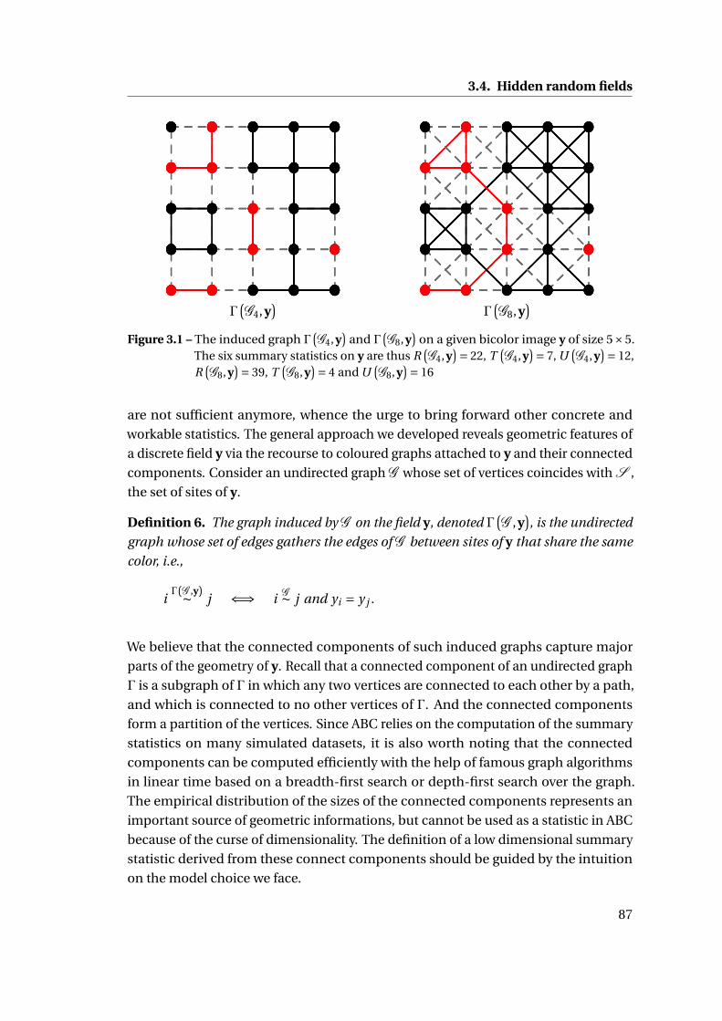
3.4. Hidden random fields
Γ(G4,y
)Γ
(G8,y
)Figure 3.1 – The induced graph Γ
(G4,y
)and Γ
(G8,y
)on a given bicolor image y of size 5×5.
The six summary statistics on y are thus R(G4,y
)= 22, T(G4,y
)= 7, U(G4,y
)= 12,R
(G8,y
)= 39, T(G8,y
)= 4 and U(G8,y
)= 16
are not sufficient anymore, whence the urge to bring forward other concrete and
workable statistics. The general approach we developed reveals geometric features of
a discrete field y via the recourse to coloured graphs attached to y and their connected
components. Consider an undirected graph G whose set of vertices coincides with S ,
the set of sites of y.
Definition 6. The graph induced by G on the field y, denoted Γ(G ,y
), is the undirected
graph whose set of edges gathers the edges of G between sites of y that share the same
color, i.e.,
iΓ(G ,y)∼ j ⇐⇒ i G∼ j and yi = y j .
We believe that the connected components of such induced graphs capture major
parts of the geometry of y. Recall that a connected component of an undirected graph
Γ is a subgraph of Γ in which any two vertices are connected to each other by a path,
and which is connected to no other vertices of Γ. And the connected components
form a partition of the vertices. Since ABC relies on the computation of the summary
statistics on many simulated datasets, it is also worth noting that the connected
components can be computed efficiently with the help of famous graph algorithms
in linear time based on a breadth-first search or depth-first search over the graph.
The empirical distribution of the sizes of the connected components represents an
important source of geometric informations, but cannot be used as a statistic in ABC
because of the curse of dimensionality. The definition of a low dimensional summary
statistic derived from these connect components should be guided by the intuition
on the model choice we face.
87

Chapter 3. ABC model choice for hidden Gibbs random fields
Our numerical experiments discriminate between a G4- and a G8-neighborhood struc-
ture and we considered two induced graphs on each simulated y, namely Γ(G4,y
)and Γ
(G8,y
). Remark that the two-dimensional statistics proposed by Grelaud et al.
(2009), which are sufficient in the noise-free context, are the total numbers of edges
in both induced graphs. After very few trials without success, we fixed ourselves on
four additional summary statistics, namely the size of the largest component of each
induced graph, as well as the total number of connect components in each graph. See
Fig. 3.1 for an example on a bicolor picture y. To fix the notations, for any induced
graph Γ(G ,y
), we define
• R(G ,y
)as the total number of edges in Γ
(G ,y
),
• T(G ,y
)as the number of connected components in Γ
(G ,y
)and
• U(G ,y
)as the size of the largest connected component of Γ
(G ,y
).
And to sum up the above, the set of summary statistics that where registered in the
reference tables for each simulated field y is
S(y) ={
R(G4,y
);R
(G8,y
);T
(G4,y
);T
(G8,y
);U
(G4,y
);U
(G8,y
)}in the first and second experiments.
In the third experiment, the observed field y takes values in R and we cannot apply
directly the approach based on induced graphes because no two pixels share the same
color. All of the above statistics are meaningless, including the statistics R(G ,y
)used
by Grelaud et al. (2009) in the noise-free case. We rely on a quantization preprocessing
performed via a kmeans algorithm on the observed colors that forgets the spatial
structure of the field. The algorithm was tuned to uncover the same number of groups
of colors as the number of latent colors, namely K = 2. If q2(y) denotes the resulting
field, the set of summary statistics becomes
S(y) ={
R(G4, q2(y)
);R
(G8, q2(y)
);T
(G4, q2(y)
);
T(G8, q2(y)
);U
(G4, q2(y)
);U
(G8, q2(y)
)}.
We have assumed here that the number of latent colors is known to keep the same
purpose of selecting the correct neighborhood structure. Indeed Cucala and Marin
88

3.4. Hidden random fields
(2013) have already proposed a (complex) Bayesian method to infer the appropriate
number of hidden colors. But more generally, we can add statistics based on various
quantizations qk (y) of y with k groups.
3.4.3 Numerical results
In all three experiments, we compare three nested sets of summary statistics S2D (y),
S4D (y) and S6D (y) of dimension 2, 4 and 6 respectively. They are defined as the
projection onto the first two (respectively four and six) axes of S(y) described in the
previous section. We stress here that S2D (y), which is composed of the summaries
given by Grelaud et al. (2009), are used beyond the noise-free setting where they are
sufficient for model choice. In order to study the information carried by the connected
components, we add progressively our geometric summary statistics to the first set,
beginning by the T(G ,y
)-type of statistics in S4D (y). Finally, remark that, before
evaluating the Euclidean distance in ABC algorithms, we normalize the statistics in
each reference tables with respect to an estimation of their standard deviation since all
these summaries take values on axis of different scales. Simulated images have been
drawn thanks to the Swendsen and Wang (1987) algorithm. In the least favourable
experiment, simulations of one hundred pictures (on pixel grid of size 100×100) via
20,000 iterations of this Markovian algorithm when parameters drawn from our prior
requires about one hour of computation on a single CPU with our optimized C++ code.
Hence the amount of time required by ABC is dominated by the simulations of y via
the Swedsen-Wang algorithm. This motivated Moores, Drovandi, Mengersen, and
Robert (2015) to propose a cut down on the cost of running an ABC experiment by
removing the simulation of an image from hidden Potts model, and replacing it by an
approximate simulation of the summary statistics. Another alternative is the clever
sampler of Mira et al. (2001) that provides exact simulations of Ising models and can
be extended to Potts models.
First experiment. Fig. 3.2(a) illustrates the calibration of the number of nearest
neighbors (parameter k of Algorithm 10) by showing the evolution of the prior error
rates (evaluated on a validation reference table including 20,000 simulations) when k
increases. We compared the errors of six classifiers to inspect the differences between
the three sets of summary statistics (in yellow, green and magenta) and the impact
of the size of the training reference table (100,000 simulations in solid lines; 50,000
simulations in dashed lines). The numerical results exhibit that a good calibration
of k can reduce the prior misclassification error. Thus, without really degrading the
performance of the classifiers, we can reduce the amount of simulations required in
89

Chapter 3. ABC model choice for hidden Gibbs random fields
0 100 200 300 400 500 600
0.00
0.02
0.04
0.06
0.08
0.10
Err
or
dim 2
dim 4
dim 6
(a)
0 100 200 300 400 500 600
0.00
0.05
0.10
0.15
0.20
0.25
0.30
0.35
dim 2 dim 4 dim 6
(b)
0.0
0.2
0.4
0.6
0.8
1.0
(c)
Figure 3.2 – First experiment results. (a) Prior error rates (vertical axis) of ABC with respectto the number of nearest neighbors (horizontal axis) trained on a reference tableof size 100,000 (solid lines) or 50,000 (dashed lines), based on the 2D, 4D and 6Dsummary statistics. (b) Prior error rates of ABC based on the 2D summary statisticcompared with 4D and 6D summary statistics including additional ancillarystatistics. (c) Evaluation of the local error on a 2D surface.
the training reference table, whose computation cost (in time) represents the main
obstacle of ABC methods, see also Table 3.1. Moreover, as can be guessed from
Fig. 3.2(a), the sizes of the largest connected components of induced graphs (included
only in S6D (y)) do not carry additional information regarding the model choice and
Table 3.1 confirms this results through evaluations of the errors on a test reference
table of 30,000 simulations drawn independently of both training and validation
reference tables.
90

3.4. Hidden random fields
Table 3.1 – Evaluation of the prior error rate on a test reference table of size 30,000 in the firstexperiment.
Prior error rates
Train size 5,000 100,000
2D statistics 8.8% 7.9%4D statistics 6.5% 6.1%6D statistics 7.1% 7.1%
Adaptive ABC 6.2% 5.5%
One can argue that the curse of dimensionality does not occur with such low dimen-
sional statistics and sizes of the training set, but this intuition is wrong, as shown in
Fig. 3.2(b). The latter plot shows indeed the prior misclassification rate as a function
of k when we replace the last four summaries by ancillary statistics drawn indepen-
dently of m and y. We can conclude that, although the three sets of summary statistics
carry then the same information in this artificial setting, the prior error rates increase
substantially with the dimension (classifiers are not trained on infinite reference ta-
bles!). This conclusion shed new light on the results of Fig. 3.2(a): the U(G ,y
)-type
summaries, based on the size of the largest component, are not concretely able to
help discriminate among models, but are either highly correlated with the first four
statistics; or the resolution (in terms of size of the training reference table) does not
permit the exploitation of the possible information they add.
Fig. 3.2(c) displays the local error rate with respect to a projection of the image space on
a plan. We have taken here S1(y) = S2D (y) in Definition 5. And S2(y) ranges a plan given
by a projection of the full set of summaries that has been tuned empirically in order to
gather the errors committed by calls of m(S2D (y)) on the validation reference table.
The most striking fact is that the local error rises above 0.9 in the oval, reddish area
of Fig. 3.2(c). Other reddish areas of Fig. 3.2(c) in the bottom of the plot correspond
to parts of the space with very low probability, and may be a dubious extrapolation
of the Kriging algorithm. We can thus conclude that the information of the new
geometric summaries depends highly on the position of y in the image space and
have confidence in the interest of Algorithm 12 (adaptive ABC) in this framework. As
exhibited in Table 3.1(d), this last classifier does not decrease dramatically the prior
misclassification rates. But the errors of the non-adaptive classifiers are already low
and the error of any classifier is bounded from below, as explained in Proposition 3.3.
Interestingly though, the adaptive classifier relies on m(S2D (y)) (instead of the most
informative m(S6D (y))) to take the final decision at about 60% of the images of our
test reference table of size 30,000.
91

Chapter 3. ABC model choice for hidden Gibbs random fields
Table 3.2 – Evaluation of the prior error rate on a test reference table of size 20,000 in thesecond experiment.
Prior error rates
Train size 50,000 100,000
2D statistics 4.5% 4.4%4D statistics 4.6% 4.1%6D statistics 4.6% 4.3%
Second experiment. The framework was designed here to study the limitations of
our approach based on the connected components of induced graphs. The number
of latent colors is indeed relatively high and the noise process do not rely on any
ordering of the colors to perturbate the pixels. Table 3.2 indicates the difficulty of
capturing relevant information with the geometric summaries we propose. Only the
sharpness introduced by a training reference table composed of 100,000 simulations
distinguishes m(S4D (y)) and m(S6D (y)) from the basic classifier m(§2D (y)). This con-
clusion is reinforced by the low value of number of neighbors after the calibration
process, namely k = 16, 5 and 5 for m(S2D (y)), m(S4D (y)) and m(S6D (y)) respectively.
Hence we do not display in this Chapter other diagnosis plots based on the prior error
rates or the conditional error rates, which led us to the same conclusion. The adaptive
ABC algorithm did not improve any of these results.
Third experiment. The framework here includes a continuous noise process as
described at the end of Section 3.4.1. We reproduced the entire diagnosis process
performed in the first experiment and we obtained the results given in Fig. 3.3 and
Table 3.3. The most noticeable difference is the extra information carried by the
U(G ,y
)-statistics, representing the size of the largest connected component, and the
adaptive ABC relies on the simplest m(S2D (y)) in about 30% of the data space (mea-
sured with the prior marginal distribution in y). Likewise, the gain in misclassification
errors is not spectacular, albeit positive.
Table 3.3 – Evaluation of the prior error rate on a test reference table of size 30,000 in the thirdexperiment.
Prior error rates
Train size 5,000 100,000
2D statistics 14.2% 13.8%4D statistics 10.8% 9.8%6D statistics 8.6% 6.9%
Adaptive ABC 8.2% 6.7%
92

3.4. Hidden random fields
0 100 200 300 400 500 600
0.00
0.05
0.10
0.15
Err
or
dim 2
dim 4
dim 6
(a)
0 100 200 300 400 500 600
0.0
0.1
0.2
0.3
0.4
dim 2 dim 4 dim 6
(b)
−0.2
0.0
0.2
0.4
0.6
0.8
(c)
Figure 3.3 – Third experiment results. (a) Prior error rates (vertical axis) of ABC with respectto the number of nearest neighbors (horizontal axis) trained on a reference tableof size 100,000 (solid lines) or 50,000 (dashed lines), based on the 2D, 4D and6D summary statistics. (b) Prior error rates of ABC based on the 2D summarystatistics compared with 4D and 6D summary statistics including additionalancillary statistics. (c) Evaluation of the local error on a 2D surface.
93


4 Model choice criteria for hiddenGibbs random field
Throughout Chapter 3, the number of latent states K was assumed to be known but in
many concrete situation this is not the case. Shaped by the development of Geman
and Geman (1984) and Besag (1986), hidden Markov random fields have enjoyed
great success in image segmentation, where one aims at estimating an unknown
class assignment from the observation of a noisy copy of a latent random field. In
this Chapter, we are interested in the joint selection of the dependency structure
and the number of latent states of a hidden Potts model. The Bayesian Information
Criterion (BIC, Schwarz, 1978) is an asymptotical estimate of the evidence that allows
to answer the question from a Bayesian viewpoint but its exact computation within the
context of hidden Markov random field is not feasible due to the intrinsic challenges
of intractable likelihoods. Up to our knowledge, few attention has been paid to this
specific issue in the literature aside from the work of Stanford and Raftery (2002)
and Forbes and Peyrard (2003). The solution of Forbes and Peyrard (2003) derives
from mean field theory which approximates the Markov random field by a system
of independent variables whose distributions are fully tractable. This approach has
proven great efficiency as regards to parameter estimation (Celeux et al., 2003) but
surprisingly encounters difficulties to select a number of latent states. We could have
also mentioned the suggestion of Cucala and Marin (2013) but from an Integrated
Completed Likelihood estimation point of view. Nevertheless their complex algorithm
is time consuming and cannot be easily extended to wider scope such as the choice of
a dependency graph.
In this chapter, we propose approximations of BIC. The general approach described
in Section 4.1 is to replace the intractable Gibbs distribution with a system of indepen-
dent random vectors, namely blocks of the lattice, by taking advantage of the recursive
algorithm of Section 1.3. To illustrate the performance of our approximations of BIC,
in Section 4.3 we focus on three different experiments on simulated data. In particular
95

Chapter 4. Model choice criteria for hidden Gibbs random field
we address the question of the selection of the number of colors and the neighbor-
hood system of a hidden Potts model. We conclude the numerical part of this Chapter
with a comparison between the ABC procedures of Chapter 3 and our model choice
criterion.
4.1 Block Likelihood Information Criterion
4.1.1 Background on Bayesian Information Criterion
The Bayesian Information Criterion offers a mean arising from Bayesian viewpoint to
select a statistical model. This Section is a brief reminder on the construction of BIC
and we refer the reader for instance to Raftery (1995) for a more detailed presentation.
We are given n independent and identically distributed observations y = {y1, . . . , yn
}from an unknown statistical model to estimate. The Bayesian approach to model
selection is based on posterior model probabilities. Consider a finite set of models
{m : 1, . . . , M } where each one is defined by a probability density function πm related
to a parameter spaceΘm . The model that best fits an observation y is the model with
the highest posterior probability
π(m
∣∣ y)= π(m)e
(y
∣∣ m)∑
m′ π(m′)e(y
∣∣ m′) ,
where e(y
∣∣ m)
denotes the evidence of m, that is the joint distribution of (y,θm)
integrated over space parameterΘm
e(y
∣∣ m)= ∫
πm(y
∣∣ θm)πm (θm)dθm .
Under the assumption of model being equally likely a priori, it is equivalent to choose
the model with the largest evidence.
BIC is an asymptotical estimate of the evidence based on Laplace method for integral
(e.g., Schwarz, 1978, Tierney and Kadane, 1986, Raftery, 1995) defined by
−2loge(y
∣∣ m)' BIC(m) =−2logπm
(y
∣∣ θMLE)+dm log(n), (4.1)
where θMLE is the maximum likelihood estimator of πm and dm is the number of free
parameters for model m. The dm log(n) term corresponds to a penalty term which
increases with the complexity of the model. Thus selecting the model with the largest
evidence is equivalent to choose the model which minimizes BIC.
96

4.1. Block Likelihood Information Criterion
The definition of BIC derives from the following result for which proof can be found,
amongst others, in the orignal paper of Schwarz (1978). We refer also the reader to
Tierney and Kadane (1986) for a formalization of some of the arguments.
Proposition 4.2. Under regularity conditions, the evidence of model m can be written
as
loge(y
∣∣ m)= logπm
(y
∣∣ θMLE)− dm
2log(n)+Rm
(θMLE
)+O(n− 1
2
), (4.2)
where Rm is bounded as the sample size grows to infinity.
Proof. Consider the Taylor series expansion of gm(θ) = log{πm(y | θ)πm(θm)
}about
the posterior mode, that is about the value θ∗ that maximizes g (θ). The expansion
writes as
gm(θ) = gm(θ∗
)+ 1
2
(θ−θ∗)T ∇2 gm
(θ∗
)(θ−θ∗)+o
(∥∥θ−θ∗∥∥).
It follows from the Laplace method for integrals applied to e(y
∣∣ m)= ∫
exp{
gm(θ))
dθ
that
e(y
∣∣ m)= logπm
(y
∣∣ θ∗)+ logπm(θ∗
)+ dm
2log(2π)− 1
2det(Am)+O
(n−1) , (4.3)
where Am =−∇2gm (θ∗).
The idea now is that in large samples θ∗ can be approximated with the maximum
likelihood estimator θMLE and the Hessian matrix Am with n times the Fisher infor-
mation matrix I(θMLE
)for one observation, that is Am = nI
(θMLE
)where I
(θMLE
) =−E
{∇2 logπm(Y1 | θMLE
)}, the expectation being taken with respect to the density of
Y1. Hence the determinant of the Hessian matrix taken at the maximum likelihood es-
timator can be estimated by det(Am) ≈ ndm det(I(θMLE
)). These two approximations
lead to an O(n− 1
2
)error into equation (4.3).
The result immediately follows with
Rm(θMLE
)= logπm(θ∗
)+ dm
2log(2π)− 1
2det
(I(θMLE
)).
Proposition 4.2 means that regardless of the prior on parameter, the error is, in general,
solely bounded and does not go to zero even with an infinite amount of data. The
approximation may hence seem somewhat crude. However as observed by Kass and
Raftery (1995) the criterion does not appear to be qualitatively misleading as long as
97

Chapter 4. Model choice criteria for hidden Gibbs random field
the sample size n is much larger than the number dm of free parameters in the model.
In addition, a reasonable choice of the prior can lead to much smaller error. Indeed,
Kass and Wasserman (1995) have found that the error is O(n−1/2
)for a well chosen
multivariate normal prior distribution.
BIC can be defined beside the special case of independent random variables. In the
latter case the approximations at the core of the proof of Proposition 4.2 are slightly
different and the number of free parameter is, in general, not equal to the dimension
of the parameter space as for the independent case. The consistency of BIC has
been proven in various situations such as independent and identically distributed
processes from the exponential families (Haughton, 1988), mixture models (Keribin,
2000), Markov chains (Csiszár et al., 2000, Gassiat, 2002) and Markov random fields
for the selection of a neighborhood system (Csiszár and Talata, 2006).
When dealing with Markov random fields, penalized likelihood criteria like BIC faces
the problem of an intractable likelihood. In addition to this issue that has been widely
underlined in this dissertation, the number of free parameters in the penalty term has
no simple formula. In the context of selecting a neighborhood system, Csiszár and
Talata (2006) proposed to replace the likelihood by the pseudolikelihood and modify
the penalty term as the number of all possible configurations for the neighboring sites.
The resulting criterion is shown to be consistent as regards this model choice.
Up to our knowledge such a result has not been yet derived for hidden Markov random
field for which another challenge appears as the incomplete likelihood requires to
integrate over the latent
πm(y
∣∣ θ)= ∫Xπ
(y
∣∣ x,φ)π
(x
∣∣β,G)µ(dx). (4.4)
The problem of approximating BIC could be once again termed a triple intractable
problem since neither the maximum likelihood estimate θMLE nor the incomplete
likelihood πm(· | θ) can be computed with standard methods and no simple definition
of dm is available.
Newton and Raftery (1994) tackled the issue of approximating BIC with an importance
sampling procedure to supersede the crude Monte Carlo estimate based on compu-
tation over all realisations of a Markov chain with stationary distribution π(· |ψ,G ).
Such an approach could have been set up here by considering the likelihood of the
conditional field π(· | y,θ,G ) as an importance sampling function but follows time
consuming procedure that we have decided not to pursue. In what follows, we rather
focus on approximations of the criterion based on approximations of the Gibbs dis-
tribution such as the pseudolikelihood (Stanford and Raftery, 2002) or the mean
98

4.1. Block Likelihood Information Criterion
field-like approximations (Forbes and Peyrard, 2003).
4.2.1 Gibbs distribution approximations
The alternate proposal to simulation methods is to replace the Gibbs distribution by
an approximation. As for the pseudolikelihood (Besag, 1975), the main idea consists
in replacing the original Markov distribution by a product easier to deal with. But
while pseudolikelihood is not a genuine probability distribution for Gibbs random
field, the focus hereafter is solely on valid probability function by considering system
of independent variables. This choice is motivated by the observations of Chapter 2
that at finite sample size, misspecification of the model has to be taken into account,
so that constant terms may appear in the remainder Rm of Proposition 4.2.
Finding good approximations of the Gibbs distribution has long standing antecedents
in statistical mechanics when one aims at predicting the response to the system to
a change in the Hamiltonian. One important technique is based on a variational
approach as the minimizer of the free energy, sometimes referred to as variational or
Gibbs free energy, defined with the Kullback-Leibler divergence between P and the
target distribution π(· |ψ,G ) as
F (P) =− log Z(ψ,G
)+KL(P,π(· |ψ,G )
). (4.5)
The Kullback-Leibler divergence being non-negative and zero if and only if P =π(· |ψ,G ), the free energy has an optimal lower bound achieved for P =π(· |ψ,G ). Mini-
mizing the free energy with respect to the set of probability distribution on X allows
to recover the Gibbs distribution but presents the same computational intractability.
A solution is to minimize the Kullback-Leibler divergence over a restricted class of
tractable probability distribution on X . This is the basis of mean field approaches
that aim at minimizing the Kullback-Leibler divergence over the set of probability
functions that factorize on sites of the lattice (see also Section 1.8.3). The minimiza-
tion of (4.5) over this set leads to fixed point equations for each marginal of P (see for
example Jordan et al., 1999).
Instead of considering distributions that completely factorize on single sites, we are
interested in tractable approximations that factorize over larger sets of nodes, namely
blocks of the lattice. Consider a partition of S into contiguous rectangular blocks,
namely
S =C⊔`=1
A(`),
99
Chapter 4. Model choice criteria for hidden Gibbs random field
and denote D the class of independent probability distributions P that factorize with
respect to this partition, that is if XA(`) =∏
i∈A(`) Xi stands for the configuration space
of the block A(`), for all x in X
P(x) =C∏`=1
P`(xA(`)
), where P` ∈M+
1
(XA(`)
)and P ∈M+
1 (X ).
Our proposal is to derive BIC approximations by replacing the intractable Gibbs
distribution with a well chosen probability distribution in D .
To take over from the Gibbs likelihood, we propose probability distribution of the
form
P(x
∣∣ x, A(1), . . . , A(C ),ψ)= C∏
`=1π
(xA(`)
∣∣ XB(`) = xB(`),ψ,G)
, (4.6)
where x is a constant field in X to specify and B(`) is either the border of A(`), i.e.,
elements of the absolute complement of A(`) that are connected to elements of A(`)
in G , or the empty set. In the latter case, we are cancelling the edges in G that link
elements of A(`) to elements of any other subset of S such that the factorization is
independent of x. The Gibbs distribution is simply replaced by the product of the
likelihood restricted to A(`). For instance a Potts model on X is replaced with a
product of Potts models on XA(`). To underline that point, x is omitted in what follows
when B(`) = ;. Note that the composite likelihood (2.1) differs from (4.6) in most
cases since blocks are not allowed to overlap and contrary to conditional composite
likelihoods, neighbors are set to constants. The only example of composite likelihoods
that lies in D is marginal composite likelihoods for non overlapping blocks.
The assumption of independent blocks leads to tractable BIC approximations. Indeed,
plugging the probability distribution (4.6) in place of the Gibbs distribution in (4.4)
yields
Pm(y
∣∣ x,θ)= ∑
x∈X
π(y
∣∣ x,φ)
P(x
∣∣ x, A(1), . . . , A(C ),ψ)
=C∏`=1
∑xA(`)
{ ∏i∈A(`)
π(yi
∣∣ xi ,φ)}π
(xA(`)
∣∣ XB(`) = xB(`),ψ,G)
=C∏`=1
∑xA(`)
π(yA(`)
∣∣ xA(`),φ)π
(xA(`)
∣∣ XB(`) = xB(`),ψ,G)
. (4.7)
This estimate of the incomplete likelihood πm(· | θ) leads to the following BIC approxi-
100

4.1. Block Likelihood Information Criterion
mations
BIC(m) ≈−2logPm(y
∣∣ x,θ∗)+dm log(|S |) := BLIC x (
m∣∣ θ∗)
, (4.8)
where θ∗ = (φ∗,ψ∗)
is a parameter value to specify. We refer to these approximations
as Block Likelihood Information Criterion (BLIC). In the first instance, the number
of free parameters dm is set to the dimension of Θm , that is we are neglecting the
interaction between variables within a block in the penalty term.
Our proposal relies on that each term of the product (4.7) can be computed using the
recursion of Friel and Rue (2007) as long as the blocks are small enough (see Section
1.3). Indeed for models whose potential linearly depends on the parameter, that is
H (x |ψ,G ) =ψT S(x) with S a vector of sufficient statistics, the probability distribution
on A(`) can be written as a Gibbs distribution on the block conditioned on the fixed
border xB(`), namely
π(xA(`)
∣∣ XB(`) = xB(`),ψ,G)= 1
Z(ψ,G , xB(`)
) exp(ψT S
(xA(`)
∣∣ x))
,
where S(xA(`)
∣∣ x)
is the restriction of S to the subgraph defined on the set A(`) and
conditioned on the fixed border xB(`) (see Example 2.1.1). Assuming that all the
marginals of the emission distribution are positive, it follows
∑xA(`)
π(yA(`)
∣∣ xA(`),φ)π
(xA(`)
∣∣ XB(`) = xB(`),ψ,G)
= 1
Z(ψ,G , xB(`)
) ∑xA(`)
exp{logπ
(yA(`)
∣∣ xA(`),φ)+ψT S
(xA(`)
∣∣ x)}
︸ ︷︷ ︸=Z (θ,G ,yA(`),xB(`))
.
The term Z(θ,G ,yA(`), xB(`)
)corresponds to the normalizing constant of the condi-
tional random field XA(`) knowing YA(`) = yA(`) and XB(`) = xB(`), that is the initial
model with an extra potential on singletons. Then the algebraic simplification at the
core of Algorithm 3 applies for both normalizing constants, such that we can exactly
compute the Block Likelihood Information Criterion, namely
BLIC x (m
∣∣ θ∗)=−2C∑`=1
{log Z
(θ∗,G ,yA(`), xB(`)
)− log Z
(ψ∗,G , xB(`)
)}+dm log(|S |). (4.9)
101

Chapter 4. Model choice criteria for hidden Gibbs random field
4.2.2 Related model choice criteria
This approach encompasses the Pseudolikelihood Information Criterion (PLIC, (1.38))
of Stanford and Raftery (2002) as well as the mean field-like approximations BICMF-like
(1.37) proposed by Forbes and Peyrard (2003) (see Section 1.8.3). When one considers
the finest partition of S , that is distributions that factorize on sites, they have already
proposed ingenious solutions for choosing x and estimating θMLE in (4.8). Indeed,
Stanford and Raftery (2002) suggest to set (x, θMLE) to the final estimates (θICM, xICM)
of the unsupervised Iterated Conditional Modes (ICM, Besag, 1986) algorithm, while
Forbes and Peyrard (2003) put forward the use of the output (θMF-like, xMF-like) of the
simulated field algorithm of Celeux et al. (2003) (see Algorithm 5 in Section 1.5.2). To
make this statement clear, we could note
PLIC(m) = BLIC xICM (m
∣∣ θICM),
BICMF-like(m) = BLIC xMF-like(m
∣∣∣ θMF-like)
.
Whilst PLIC shows good result as regards the selection of the number of components
of the hidden state, ICM performs poorly for the parameter estimation in comparison
with the EM-like algorithm of Celeux et al. (2003). Hence we advocate in favour of the
latter in what follows to get estimates of θMLE and to fix a segmented random field x.
We shall also remark that for a factorization over the graph nodes when B(`) = ;we retrieve a mixture model. Indeed, turning off all the edges in G leads to approxi-
mate the Gibbs distribution by a multinomial distribution with event probabilities
depending on the potential on singletons. Hence if marginal emission distribution are
Gaussian random variables depending on the component on the latent site associated,
we would deal with a classical Gaussian mixture model.
4.3 Comparison of BIC approximations
Our primary intent with the BIC approximations exposed in Section 4.1 was to choose
the number of latent states and a dependency structure of a hidden Markov random
fields. The following numerical experiments illustrate the performances as regards
these questions for realizations of a hidden Potts model. Section 4.3.2 and Section
4.3.3 focus on a comparison between the different criteria to discriminate between
hidden models in various settings while Section 4.3.4 presents a comparison with the
ABC procedures introduced in Chapter 3.
102

4.3. Comparison of BIC approximations
4.3.1 Hidden Potts models
This numerical part of the Chapter focuses on observations for which the hidden
field is modelled by a K -states Potts model parametrized by ψ≡β. The model sets a
probability distribution on X = {1, . . . ,K }n defined by
π(x
∣∣β,G)= 1
Z(β,G
) exp
β∑iG∼ j
1{
xi = x j} .
We set the emission law π(y | x,φ) =∏i∈S π(yi | xi ,φ), such that the marginal distribu-
tion are Gaussian distribution depending on the related latent state, namely
yi | xi = k ∼N(µk ,σ2
k
)k ∈ {0, . . . ,K −1},
where µk is the mean and σk is the standard deviation for sites belonging to class k.
The parameter to be estimated with the ICM or simulated field algorithms is then
θ = (φ,β
), with φ= {(
µk ,σk)
: k = 0, . . . ,K −1}
.
We denote HPM(G ,θ,K ), the hidden K-states Potts model defined above.
The common point of our examples is to select the hidden Potts model that better fits
a given observation yobs composed of n = 100×100 pixels among a collection
M = {HPM(G ,θ,K ) : K = Kmin, . . . ,Kmax ; G ∈ {
G4,G8}}
,
where K is the number of colors of the corresponding model and G is one of the
two possible neighborhood systems: G4 and G8 defined in Chapter 1, see Figure 1.1.
For each model HPM(G ,θ,K ), the estimate θMLE and the segmented field x were
computed using SpaCEM3 (see the Documentation on http://spacem3.gforge.inria.fr).
The software allows the implementation of the unsupervised ICM algorithm as well as
the simulated field algorithm and provides computation of PLIC, the mean field-like
approximations BICMF-like and BICGBF (Equation (1.40)). The ICM and the EM-like
algorithms were both initialized with a simple K -means procedure. The stopping
criterion is then settled to a number of 200 iterations that is enough to ensure the
convergence of the procedure.
In what follows, we restrict each A(`) to be of the same dimension and in particular
square block of dimension b ×b. For the sake of clarity the Block Likelihood Criterion
is indexed by the dimension of the blocks, namely for a partition of square blocks of
size b ×b for which x = xMF-like and θMLE = θMF-like, we note it BLICMF-likeb×b . As already
103

Chapter 4. Model choice criteria for hidden Gibbs random field
mentioned, we then have BICMF-like = BLICMF-like1×1 . We recall that when B(`) =;, x is
omitted in the previous notations, that is for a square blocks partition we note our
criterion BLICb×b . Then BLIC1×1 is the BIC approximations corresponding to a finite
independent mixture model. All criterion were tested on simulated images obtained
using the Swendsen-Wang algorithm. We describe below the different experiments
settings we have considered and the results we got.
4.3.2 First experiment: selection of the number of colors
We considered realizations from hidden Potts models with KT = 4 colors. We carried
out 100 simulations from the first order neighborhood structure G4 and 100 simu-
lations from the second order neighborhood structure G8. In this experiment the
dependency structure is assumed to be known and the aim is to recover the number
K of colors of the latent configuration. The interaction parameter β was set close
to the phase transition, namely β = 1 and β = 0.4 for G4 and G8 respectively. These
values of the parameter ensure the images present homogeneous regions and then the
observations exhibit some spatial structure. Such settings illustrate the advantage of
taking into account spatial information of the model. Obviously, for values of β where
the interaction is weaker, the benefit of the criterion that include the dependency
structure of the model is not clear. The latter could even be misleading in comparison
with BIC approximations for independent mixture models when β is close to zero. On
the other side, when β is above the phase transition, the distribution on X becomes
heavily multi-modal and there is almost solely one class represented in the image
regardless the number of colors of the model.
The noise process is a homoscedastic Gaussian noise centered at the value of the
related nodes, namely
yi | xi = k ∼N(k,σ2
k
)k ∈ {0, . . . ,K −1},
where σk = 0.5 for k = 1, . . . ,K . Even though the noise model is homoscedastic, we still
index the standard deviation by k since we do not use the assumption of a constant
variance in the estimation procedure, such that the number of parameters estimated
is dm = 2×k +1.
The results obtained for the different criterion are reported in Table 4.1. For b ≥ 2,
BLICb×b outperform the different criterion even though PLIC and BLIC1×1 provide
good results. By contrast approximations based on mean field-like approximations,
that is BICMF-like, BICGBF and BLICMF-like2×2 , perform poorly. These conclusions need
nonetheless to be put into perspective. Figure 4.1(a) shows that the main issue encoun-
104
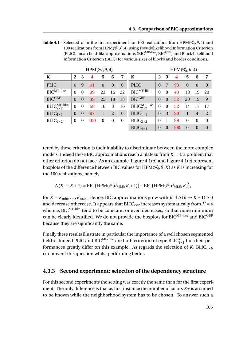
4.3. Comparison of BIC approximations
Table 4.1 – Selected K in the first experiment for 100 realizations from HPM(G4,θ,4) and100 realizations from HPM(G8,θ,4) using Pseudolikelihood Information Criterion(PLIC), mean field-like approximations (BICMF-like, BICGBF) and Block LikelihoodInformation Criterion (BLIC) for various sizes of blocks and border conditions.
HPM(G4,θ,4)
K 2 3 4 5 6 7
PLIC 0 9 91 0 0 0
BICMF-like 0 0 39 23 16 22
BICGBF 0 0 39 25 18 18
BLICMF-like2×2 0 0 58 18 8 16
BLIC1×1 0 0 97 1 2 0
BLIC2×2 0 0 100 0 0 0
HPM(G8,θ,4)
K 2 3 4 5 6 7
PLIC 0 7 93 0 0 0
BICMF-like 0 0 43 18 19 20
BICGBF 0 0 52 20 19 9
BLICMF-like2×2 0 0 52 14 17 17
BLIC1×1 0 3 90 1 4 2
BLIC2×2 0 1 99 0 0 0
BLIC4×4 0 0 100 0 0 0
tered by these criterion is their inability to discriminate between the more complex
models. Indeed these BIC approximations reach a plateau from K = 4, a problem that
other criterion do not face. As an example, Figure 4.1(b) and Figure 4.1(c) represent
boxplots of the difference between BIC values for HPM(G4,θ,K ) as K is increasing for
the 100 realizations, namely
∆ (K → K +1) = BIC(HPM(G , θMLE,K +1)
)−BIC(HPM(G , θMLE,K )
),
for K = Kmin, . . . ,Kmax. Hence, BIC approximations grow with K if ∆ (K → K +1) ≥ 0
and decrease otherwise. It appears that BLIC2×2 increases systematically from K = 4
whereas BICMF-like tend to be constant, or even decreases, so that none minimum
can be clearly identified. We do not provide the boxplots for BICMF-like and BICGBF
because they are significantly the same.
Finally these results illustrate in particular the importance of a well chosen segmented
field x. Indeed PLIC and BICMF-like are both criterion of type BLICx1×1 but their per-
formances greatly differ on this example. As regards the selection of K , BLICb×b
circumvent this question whilst performing better.
4.3.3 Second experiment: selection of the dependency structure
For this second experiments the setting was exactly the same than for the first experi-
ment. The only difference is that as first instance the number of colors KT is assumed
to be known while the neighborhood system has to be chosen. To answer such a
105

Chapter 4. Model choice criteria for hidden Gibbs random field
2 3 4 5 6 7
2500
026
000
2700
028
000
B2[
16, ]
BIC MF−like
BIC GBF
BLIC 2x2 MF−like
(a)
−20
00−
1500
−10
00−
500
0
∆(2 → 3) ∆(3 → 4) ∆(4 → 5) ∆(5 → 6) ∆(6 → 7)
(b)
−80
0−
600
−40
0−
200
020
0
∆(2 → 3) ∆(3 → 4) ∆(4 → 5) ∆(5 → 6) ∆(6 → 7)
(c)
Figure 4.1 – First experiment results. (a) BICMF-like, BICGBF and BLICMF-like2×2 values for one
realization of a first order hidden Potts model HPM(G ,θ,4). (b) Difference be-tween BLICMF-like
2×2 values for 100 realization of a first order hidden Potts modelHPM(G4,θ,4) as K is increasing. (c) Difference between BLIC2×2 values for 100realization of a first order hidden Potts model HPM(G4,θ,4) as K is increasing
question it is obvious that we can not use criterion BLIC1×1 based on independent
mixture model.
As regards this question, all but two criterion perform very well, see Table 4.2. In the
first place, PLIC faces trouble to select the correct G4. This illustrate the importance
of the estimation of the interaction parameter β. We have observed that the ICM
algorithm whilst providing good segmented field, produces poorer estimates of the
parameter than the simulated field algorithm. This has an impact quite important
since β sets the strength of interaction between neighboring nodes of the graph G
and is most representative of the spatial correlation. On the other hand, BLIC2×2 fails
to select the neighborhood system for second order hidden Potts model HPM(G8,θ,4).
This conclusion can be simply explained by the fact that the block does not include
106
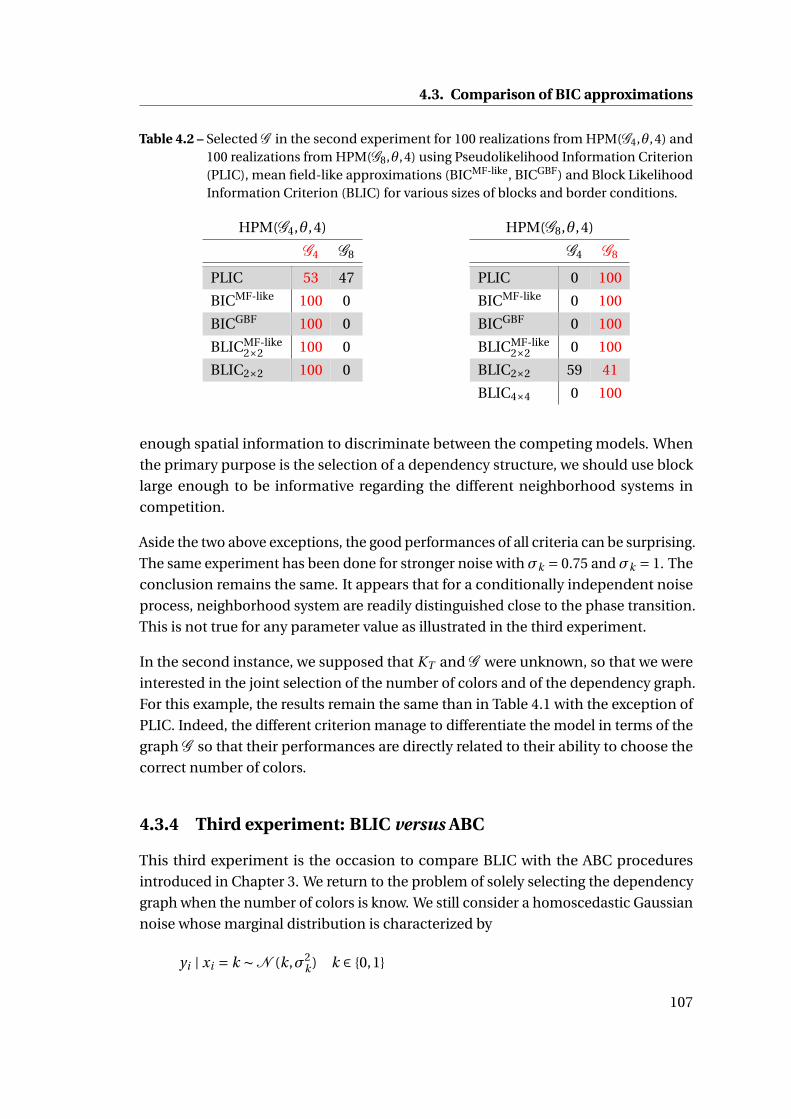
4.3. Comparison of BIC approximations
Table 4.2 – Selected G in the second experiment for 100 realizations from HPM(G4,θ,4) and100 realizations from HPM(G8,θ,4) using Pseudolikelihood Information Criterion(PLIC), mean field-like approximations (BICMF-like, BICGBF) and Block LikelihoodInformation Criterion (BLIC) for various sizes of blocks and border conditions.
HPM(G4,θ,4)
G4 G8
PLIC 53 47
BICMF-like 100 0
BICGBF 100 0
BLICMF-like2×2 100 0
BLIC2×2 100 0
HPM(G8,θ,4)
G4 G8
PLIC 0 100
BICMF-like 0 100
BICGBF 0 100
BLICMF-like2×2 0 100
BLIC2×2 59 41
BLIC4×4 0 100
enough spatial information to discriminate between the competing models. When
the primary purpose is the selection of a dependency structure, we should use block
large enough to be informative regarding the different neighborhood systems in
competition.
Aside the two above exceptions, the good performances of all criteria can be surprising.
The same experiment has been done for stronger noise withσk = 0.75 and σk = 1. The
conclusion remains the same. It appears that for a conditionally independent noise
process, neighborhood system are readily distinguished close to the phase transition.
This is not true for any parameter value as illustrated in the third experiment.
In the second instance, we supposed that KT and G were unknown, so that we were
interested in the joint selection of the number of colors and of the dependency graph.
For this example, the results remain the same than in Table 4.1 with the exception of
PLIC. Indeed, the different criterion manage to differentiate the model in terms of the
graph G so that their performances are directly related to their ability to choose the
correct number of colors.
4.3.4 Third experiment: BLIC versus ABC
This third experiment is the occasion to compare BLIC with the ABC procedures
introduced in Chapter 3. We return to the problem of solely selecting the dependency
graph when the number of colors is know. We still consider a homoscedastic Gaussian
noise whose marginal distribution is characterized by
yi | xi = k ∼N (k,σ2k ) k ∈ {0,1}
107

Chapter 4. Model choice criteria for hidden Gibbs random field
Table 4.3 – Evaluation of the prior error rate of ABC procedures and of the error rate for themodel choice criterion in the third experiment.
Train size 5,000 100,000 Criterion Error rate
2D statistics 14.2% 13.8% PLIC 19.8%
4D statistics 10.8% 9.8% BICMF-like 7.6%
6D statistics 8.6% 6.9% BICGBF 7.1%
Adaptive ABC 8.2% 6.7% BLIC4×4 7.7%
but over bicolor Potts models. The standard deviation σk = 0.39, k ∈ {0,1}, was set so
that the probability of a wrong prediction of the latent color with a marginal MAP rule
on the Gaussian model is about 10% in the thresholding step of the ABC procedure.
Regarding the dependency parameter β, we set prior distributions below the phase
transition which occurs at different levels depending on the neighborhood structure.
Precisely we used a uniform distribution over (0;1) when the adjacency is given by G4
and a uniform distribution over (0;0.35) with G8. In order to examine the performance
of model choice criteria in comparison of ABC, we carried out 1000 realizations from
HPM(G4,θ,2) and 1000 realizations from HPM(G8,θ,2) with parameters from the
priors. The results are presented in Table 4.3
The novel ABC procedure introduced in Chapter 3 appears to provide the best per-
formances but for a training reference table of size 100 000. This reinforces the idea
that for unlimited computation possibilities, ABC can efficiently address situations
where the likelihood is intractable. However, Table 4.3 suggest that for a much lower
computational cost it is possible to get equivalent, or even better, error rate by using
model choice criterion BICMF-like, BICGBF or BLICb×b , while PLIC seems not to be over-
taken. In this example, BICGBF slightly supersede BICMF-like and BLICb×b . This can be
explained by the fact that for parameter from the prior close to zero, the assumption
of independence between the sites is almost true. In the latter case, estimating BIC
using the first order approximations of the partition function of Gibbs distribution
(see the lower bound 1.39 in Section 1.8.3) may be preferable than using normalizing
constants defined on blocks.
108

Conclusion
The present dissertation addresses well-known statistical inference issues for Markov
random fields. One of our contribution concerns the calibration of approximate
Bayesian computation algorithms for model choice as a classification problem. In this
context, we have derived a local error rate that is an indicator of the gain or the loss of
statistical information induced by the summary statistics conditional on the observed
value. Consequently, we set up an adaptive classifier which is an attempt to fight
locally against the curse of dimensionality. Our approach is an advance over most
projection methods which are focused on parameter estimation (Blum et al., 2013).
While most of these techniques perform a global trade off between the dimension and
the information of the summary statistics over the whole prior domain, our proposal
allows to select, at least in theory, the optimal set of summary statistic as the one
minimizing the local error rate at the observed value. Principles of our proposal
are well founded by avoiding the well-known optimism of the training error rates
and by resorting to validation and test reference tables in order to evaluate the error
practically. Another possibility taken by Pudlo et al. (2014) is to resort to a machine
learning classifier adapted to a large number of covariates such as random forest.
Regarding latent Markov random fields, the proposed method of constructing sum-
mary statistics based on the induced graphs yields a promising route to construct
relevant summary statistics in this framework. The approach is very intuitive and
can be reproduced in other settings. For instance, if the goal is to select between
isotropic latent Gibbs models and anisotropic models, the averaged ratio between the
width and the length of the connected components or the ratio of the width and the
length of the largest connected components can be relevant numerical summaries.
We have also explained how to adapt the method to a continuous noise by performing
a quantization of the observed values at each site of the fields. The detailed analysis
of the numerical results demonstrates that the approach is promising. However the
results on the 16 color example indicate the limitation of the induced graph approach
as the number of colors grows. We believe that there exists a road we did not explore
above with an induced graph that add weights on the edges of the graph according to
109

Conclusion
the proximity of the colors, but the grouping of sites on such weighted graph is not
trivial.
The numerical results of Chapter 3 opens up new vistas regarding the calibration of
ABC algorithms. Our contribution could be especially interesting for statistical models
on high dimensional space for which ABC is the only solution available. Our work has
put this statement into perspective for hidden Markov random fields. The numerical
results in Chapter 3 highlighted that the calibration of the number of neighbors in
ABC provides better results (in terms of misclassification) than a threshold set as a
fixed quantile of the distances between the simulated and the observed datasets (as
proposed in Marin et al., 2012). Consequently, we pointed out that the shift from
posterior distribution regression to classification problem allows to reduce noticeably
the number of simulation required in the ABC reference table without increasing the
misclassification error rates. The latter represents an important conclusion since
the simulation of a latent Markov random field requires a non-negligible amount of
time. Even though the computational cost is cut down, ABC procedures remain time
consuming in comparison with methods based on approximations of the likelihood
and their relative efficiency in certain situations regarding Markov random fields
can barely justify the extra computational cost. However, mention that we run into
that problem because the computation of the summary statistics require to simulate
from the model. Following Moores et al. (2015), it would be interesting to see if
we could directly simulate the summary statistics which will reduce once again the
computational burden.
Other contributions of the present dissertation focus on possible block approxima-
tions of the Gibbs distribution. These approaches allow to circumvent the major
drawback of Monte Carlo approaches, namely their time complexity. As regards the
estimation of posterior model parameter, we have illustrated the important role con-
ditional composite likelihood approximations can play in the statistical analysis of
Markov random field, and in particular Ising and autologistic models in spatial statis-
tics, as a mean for overcoming the intractability of the likelihood function. In the
Bayesian setting, we proposed an adjustment of the mode and the curvature at the
mode of the posterior distribution as a way to correct the underestimated posterior
mean and variance resulting from the use of a composite likelihood. This work has
in particular pointed out that the main difficulty of such approaches is to handle the
misspecification induced by non genuine likelihood functions.
In a context of model section, we proposed to move towards variational methods and
in particular to use valid probability distributions in place of the intractable likelihood.
Our proposal is to consider a product of valid distributions over non-overlapping
110

blocks of the lattice. Consequently, we derived Block Likelihood Information Criterion
to discriminate between hidden Markov random fields. According to the numerical
results of Chapter 4, the opportunity appears to be a satisfactory alternative to ABC
model choice algorithms.
Perspectives
The first aspect of a further work is to scale-up all our approaches/algorithms to
lattices of much larger size. Indeed, most of the results were carried out for regular 2D-
grid of 100×100 sites. The flexibility and the ability of the approach to handle larger
graph will play a decisive role in the design of useful methodology. The extension of
the present work is not restricted to the only issue of larger graphs but can also be
studied towards Gibbs random fields with larger number of parameters, such as the
exponential random graph model particularly interesting for the analysis of social
network. In the latter case, it could be interesting to adapt the methods of Chapter 2 to
the hidden case and to study its performance as regards inference on random graph.
Another possibility yet to be explored is the robustness of the model choice approaches
to the noise process. As a motivation of the question, we observed the limitation of
the induced graph approach on the 16 colors example of Chapter 3 with a completely
disordered noise. For continuous noise model, we have made two assumptions. The
emission distribution was assumed to be first Gaussian and secondly conditionally
independent. Whilst the latter modelling is quite standard, it would be interesting
to further look noise process with heavier distribution tails such as the Student or
Cauchy distributions as well as noise process that includes spatial information.
Besides modelling and practical limitations, the dissertation has raised some other
questions. Our primary interest goes to the approximations of the Gibbs likelihood by
probability distributions that factorize over blocks of the lattice. The latter approach
offers an appealing trade-off between efficient computation and reliable results. Chap-
ter 4 has introduced a novel criterion which makes in its current version two major
approximations that are worth exploring. First mention, the choice of a particular
substitute is lead by any optimality conditions. From that viewpoint, the construction
of an optimal approximations regarding the variational free energy over the set of
probability distributions that factorize on blocks is yet to be studied. At first sight, the
existence of an explicit solution seems far from obvious. However it would be inter-
esting to study their possible relation with region-based approximations of Yedidia
et al. (2005). Their generalized belief propagation algorithms could give an estimate of
the Kullback-Leibler divergence solution to build up the intended optimal approxi-
111

Conclusion
mations. Overall, variational methods, through the development of new calculation
means, may offers reliable solution for hidden Markov random fields.
The second level of approximations concerns the penalty term. The next step of our
work cannot be reduced to the sole aim of improving the quality of the approximations.
Through Chapter 4, we have seen that an optimal solution with respect to the Kullback-
Leibler divergence is not sufficient to ensure a good behaviour of model choice criteria,
especially if the more complex model are not enough penalized. The penalty term
used is solely valid for independent variable. We have neglected the interaction within
a block, an assumption that slightly modified the number of free parameter. The
impact of dependence variables on the penalty term is a logical follow-up to our work.
112

Bibliography
H. Akaike. Information theory and an extension of the maximum likelihood princi-
ple. In Second International Symposium on Information Theory, pages 267–281.
Akademinai Kiado, 1973.
M. Alfò, L. Nieddu, and D. Vicari. A finite mixture model for image segmentation.
Statistics and Computing, 18(2):137–150, 2008.
C. Andrieu and G. O. Roberts. The Pseudo-Marginal Approach for Efficient Monte
Carlo Computations. The Annals of Statistics, 37(2):697–725, 2009.
C. Andrieu, A. Doucet, and R. Holenstein. Particle Markov Chain Monte Carlo methods.
Journal of the Royal Statistical Society: Series B (Statistical Methodology), 72(3):269–
342, 2010.
A. U. Asuncion, Q. Liu, A. T. Ihler, and P. Smyth. Learning with blocks: Composite
likelihood and contrastive divergence. In AISTATS, Journal of Machine Learning
Research: W&CP, volume 9, pages 33–40, 2010.
M. Baragatti and P. Pudlo. An overview on approximate Bayesian computation. ESAIM:
Proc., 44:291–299, 2014.
A. Barbu and S.-C. Zhu. Generalizing Swendsen-Wang to sampling arbitrary posterior
probabilities. Pattern Analysis and Machine Intelligence, IEEE Transactions on, 27
(8):1239–1253, 2005.
M. A. Beaumont. Estimation of Population Growth or Decline in Genetically Moni-
tored Populations. Genetics, 164(3):1139–1160, 2003.
M. A. Beaumont, W. Zhang, and D. J. Balding. Approximate Bayesian Computation in
Population Genetics. Genetics, 162(4):2025–2035, 2002.
M. A. Beaumont, J.-M. Cornuet, J.-M. Marin, and C. P. Robert. Adaptive approximate
Bayesian computation. Biometrika, 2009. doi: 10.1093/biomet/asp052.
113

Bibliography
J. E. Besag. Nearest-neighbour Systems and the Auto-Logistic Model for Binary Data.
Journal of the Royal Statistical Society. Series B (Methodological), 34(1):75–83, 1972.
J. E. Besag. Spatial Interaction and the Statistical Analysis of Lattice Systems (with
Discussion). Journal of the Royal Statistical Society. Series B (Methodological), 36(2):
192–236, 1974.
J. E. Besag. Statistical Analysis of Non-Lattice Data. The Statistician, 24:179–195, 1975.
J. E. Besag. On the Statistical Analysis of Dirty Pictures. Journal of the Royal Statistical
Society. Series B (Methodological), 48(3):259–302, 1986.
J. E. Besag and P. J. Green. Spatial Statistics and Bayesian Computation. Journal of the
Royal Statistical Society. Series B (Methodological), 55(1):25–37, 1993.
J. E. Besag, J. York, and A. Mollié. Bayesian image restoration, with two applications in
spatial statistics. Annals of the institute of statistical mathematics, 43(1):1–20, 1991.
G. Biau, F. Cérou, and A. Guyader. New insights into Approximate Bayesian Compu-
tation. Annales de l’Institut Henri Poincaré (B) Probabilités et Statistiques, in press,
2013.
C. Biernacki, G. Celeux, and G. Govaert. Assessing a mixture model for clustering with
the integrated completed likelihood. Pattern Analysis and Machine Intelligence,
IEEE Transactions on, 22(7):719–725, 2000.
M. G. B. Blum, M. A. Nunes, D. Prangle, and S. A. Sisson. A Comparative Review of
Dimension Reduction Methods in Approximate Bayesian Computation. Statistical
Science, 28(2):189–208, 2013.
K. P. Burnham and D. R. Anderson. Model selection and multimodel inference: a
practical information-theoretic approach. Springer Science & Business Media, 2002.
A. Caimo and N. Friel. Bayesian inference for exponential random graph models.
Social Networks, 33(1):41–55, 2011.
A. Caimo and N. Friel. Bayesian model selection for exponential random graph models.
Social Networks, 35(1):11 – 24, 2013.
G. Celeux and J. Diebolt. The SEM algorithm: a probabilistic teacher algorithm derived
from the EM algorithm for the mixture problem. Computational Statistics Quarterly,
2(1):73–82, 1985.
114

Bibliography
G. Celeux, F. Forbes, and N. Peyrard. EM procedures using mean field-like approxi-
mations for Markov model-based image segmentation. Pattern Recognition, 36(1):
131–144, 2003.
B. Chalmond. An iterative Gibbsian technique for reconstruction of m-ary images.
Pattern Recognition, 22(6):747–761, 1989.
R. E. Chandler and S. Bate. Inference for clustered data using the independence
loglikelihood. Biometrika, 94(1):167–183, 2007.
P. Clifford. Markov random fields in statistics. Disorder in physical systems: A volume
in honour of John M. Hammersley, pages 19–32, 1990.
C. Cooper and A. M. Frieze. Mixing properties of the Swendsen-Wang process on
classes of graphs. Random Structures and Algorithms, 15(3-4):242–261, 1999.
D. R. Cox and N. Reid. A note on pseudolikelihood constructed from marginal densities.
Biometrika, 91(3):729–737, 2004.
I. Csiszár and Z. Talata. Consistent Estimation of the Basic Neighborhood of Markov
Random Fields. The Annals of Statistics, 34(1):123–145, 2006.
I. Csiszár, P. C. Shields, et al. The consistency of the BIC Markov order estimator. The
Annals of Statistics, 28(6):1601–1619, 2000.
L. Cucala and J.-M. Marin. Bayesian Inference on a Mixture Model With Spatial
Dependence. Journal of Computational and Graphical Statistics, 22(3):584–597,
2013.
L. Cucala, J.-M. Marin, C. P. Robert, and D. M. Titterington. A Bayesian Reassessment
of Nearest-Neighbor Classification. Journal of the American Statistical Association,
104(485):263–273, 2009.
P. Del Moral, A. Doucet, and A. Jasra. An adaptive sequential monte carlo method for
approximate bayesian computation. Statistics and Computing, 22(5):1009–1020,
2012.
A. P. Dempster, N. M. Laird, and D. B. Rubin. Maximum Likelihood from Incom-
plete Data via the EM Algorithm. Journal of the Royal Statistical Society. Series B
(Methodological), 39(1):1–38, 1977.
X. Descombes, R. D. Morris, J. Zerubia, and M. Berthod. Estimation of Markov random
field prior parameters using Markov chain Monte Carlo maximum likelihood. Image
Processing, IEEE Transactions on, 8(7):954–963, 1999.
115

Bibliography
L. Devroye, L. Györfi, and G. Lugosi. A probabilistic theory of pattern recognition,
volume 31 of Applications of Mathematics (New York). Springer-Verlag, New York,
1996.
X. Didelot, R. G. Everitt, A. M. Johansen, and D. J. Lawson. Likelihood-free estimation
of model evidence. Bayesian Analysis, 6(1):49–76, 2011.
P. Druilhet and J.-M. Marin. Invariant HPD credible sets and MAP estimators. Bayesian
Analysis, 2(4):681–691, 2007.
R. G. Edwards and A. D. Sokal. Generalization of the Fortuin-Kasteleyn-Swendsen-
Wang representation and Monte Carlo algorithm. Physical review D, 38(6):2009,
1988.
A. Estoup, E. Lombaert, J.-M. Marin, C. Robert, T. Guillemaud, P. Pudlo, and J.-M. Cor-
nuet. Estimation of demo-genetic model probabilities with Approximate Bayesian
Computation using linear discriminant analysis on summary statistics. Molecular
Ecology Ressources, 12(5):846–855, 2012.
R. G. Everitt. Bayesian Parameter Estimation for Latent Markov Random Fields and
Social Networks. Journal of Computational and Graphical Statistics, 21(4):940–960,
2012.
F. Forbes and G. Fort. Combining Monte Carlo and Mean Field-Like Methods for
Inference in Hidden Markov Random Fields. Image Processing, IEEE Transactions
on, 16(3):824–837, 2007.
F. Forbes and N. Peyrard. Hidden Markov random field model selection criteria based
on mean field-like approximations. Pattern Analysis and Machine Intelligence, IEEE
Transactions on, 25(9):1089–1101, 2003.
O. François, S. Ancelet, and G. Guillot. Bayesian Clustering Using Hidden Markov
Random Fields in Spatial Population Genetics. Genetics, 174(2):805–816, 2006.
O. Frank and D. Strauss. Markov graphs. Journal of the American Statistical Association,
81(395):832–842, 1986.
N. Friel. Bayesian Inference for Gibbs Random Fields Using Composite Likelihoods.
In Proceedings of the Winter Simulation Conference, number 28 in WSC ’12, pages
1–8. Winter Simulation Conference, 2012.
N. Friel and A. N. Pettitt. Likelihood Estimation and Inference for the Autologistic
Model. Journal of Computational and Graphical Statistics, 13(1):232–246, 2004.
116

Bibliography
N. Friel and H. Rue. Recursive computing and simulation-free inference for general
factorizable models. Biometrika, 94(3):661–672, 2007.
N. Friel, A. N. Pettitt, R. Reeves, and E. Wit. Bayesian Inference in Hidden Markov
Random Fields for Binary Data Defined on Large Lattices. Journal of Computational
and Graphical Statistics, 18(2):243–261, 2009.
E. Gassiat. Likelihood ratio inequalities with applications to various mixtures. In
Annales de l’IHP Probabilités et statistiques, volume 38, pages 897–906, 2002.
A. Gelman and X.-L. Meng. Simulating normalizing constants: From importance
sampling to bridge sampling to path sampling. Statistical science, 13(2):163–185,
1998.
S. Geman and D. Geman. Stochastic Relaxation, Gibbs Distributions, and the Bayesian
Restoration of Images. IEEE Transactions on Pattern Analysis and Machine Intelli-
gence, 6(6):721–741, 1984.
S. Geman and C. Graffigne. Markov Random Field Image Models and Their Ap-
plications to Computer Vision. In Proceedings of the International Congress of
Mathematicians, volume 1, pages 1496–1517, 1986.
H. Georgii. Gibbs Measures and Phase Transitions. De Gruyter studies in mathematics.
De Gruyter, 2011.
C. J. Geyer. Markov Chain Monte Carlo Maximum Likelihood. 1991.
C. J. Geyer and E. A. Thompson. Constrained Monte Carlo Maximum Likelihood for
Dependent Data. Journal of the Royal Statistical Society. Series B (Methodological),
54(3):657–699, 1992.
H. Geys, M. M. Regan, P. J. Catalano, and G. Molenberghs. Two Latent Variable Risk
Assessment Approaches for Mixed Continuous and Discrete Outcomes from De-
velopmental Toxicity Data. Journal of Agricultural, Biological, and Environmental
Statistics, 6(3):340–355, 2001.
V. K. Gore and M. R. Jerrum. The Swendsen–Wang process does not always mix rapidly.
Journal of Statistical Physics, 97(1-2):67–86, 1999.
P. J. Green and S. Richardson. Hidden Markov Models and Disease Mapping. Journal
of the American Statistical Association, 97(460):1055–1070, 2002.
A. Grelaud, C. P. Robert, J.-M. Marin, F. Rodolphe, and J.-F. Taly. ABC likelihood-free
methods for model choice in Gibbs random fields. Bayesian Analysis, 4(2):317–336,
2009.
117

Bibliography
G. R. Grimmett. A theorem about random fields. Bulletin of the London Mathematical
Society, 5(1):81–84, 1973.
W. K. Hastings. Monte Carlo sampling methods using Markov chains and their appli-
cations. Biometrika, 57(1):97–109, 1970.
D. M. A. Haughton. On the Choice of a Model to Fit Data from an Exponential Family.
The Annals of Statistics, 16(1):342–355, 1988.
P. J. Heagerty and S. R. Lele. A composite likelihood approach to binary spatial data.
Journal of the American Statistical Association, 93(443):1099–1111, 1998.
J. Heikkinen and H. Hogmander. Fully Bayesian approach to image restoration with
an application in biogeography. Journal of the Royal Statistical Society. Series C
(Applied Statistics), 43(4):569–582, 1994.
D. M. Higdon. Discussion on the Meeting on the Gibbs Sampler and Other Markov
Chain Monte Carlo Methods. Journal of the Royal Statistical Society. Series B, 55(1):
78, 1993.
D. M. Higdon. Auxiliary variable methods for Markov chain Monte Carlo with applica-
tions. Journal of the American Statistical Association, 93(442):585–595, 1998.
M. Huber. A bounding chain for Swendsen-Wang. Random Structures & Algorithms,
22(1):43–59, 2003.
M. A. Hurn, O. K. Husby, and H. Rue. A Tutorial on Image Analysis. In Spatial Statistics
and Computational Methods, volume 173 of Lecture Notes in Statistics, pages 87–141.
Springer New York, 2003.
E. Ising. Beitrag zur Theorie des Ferromagnetismus. Zeitschrift fur Physik, 31:253–258,
1925.
C. Ji and L. Seymour. A consistent model selection procedure for Markov random
fields based on penalized pseudolikelihood. The annals of applied probability,
pages 423–443, 1996.
M. I. Jordan, Z. Ghahramani, T. S. Jaakkola, and L. K. Saul. An Introduction to Varia-
tional Methods for Graphical Models. Machine learning, 37(2):183–233, 1999.
R. E. Kass and A. E. Raftery. Bayes factors. Journal of the american statistical association,
90(430):773–795, 1995.
118

Bibliography
R. E. Kass and L. Wasserman. A reference Bayesian test for nested hypotheses and its
relationship to the schwarz criterion. Journal of the American Statistical Association,
90(431):928–934, 1995.
R. W. Katz. On Some Criteria for Estimating the Order of a Markov Chain. Technomet-
rics, 23(3):243–249, 1981.
J. T. Kent. Robust Properties of Likelihood Ratio Test. Biometrika, 69(1):19–27, 1982.
C. Keribin. Consistent Estimation of the Order of Mixture Models. Sankhy: The Indian
Journal of Statistics, Series A (1961-2002), 62(1):49–66, 2000.
I. Lanford, O.E. and D. Ruelle. Observables at infinity and states with short range
correlations in statistical mechanics. Communications in Mathematical Physics, 13
(3):194–215, 1969.
B. G. Lindsay. Composite likelihood methods. Contemporary Mathematics, 80(1):
221–39, 1988.
J. S. Liu. Peskun’s theorem and a modified discrete-state gibbs sampler. Biometrika,
83(3):681–682, 1996.
J.-M. Marin, P. Pudlo, C. P. Robert, and R. J. Ryder. Approximate Bayesian Computa-
tional methods. Statistics and Computing, 22(6):1167–1180, 2012.
J.-M. Marin, N. S. Pillai, C. P. Robert, and J. Rousseau. Relevant statistics for Bayesian
model choice. Journal of the Royal Statistical Society: Series B (Statistical Methodol-
ogy), 76(5):833–859, 2014.
P. Marjoram, J. Molitor, V. Plagnol, and S. Tavaré. Markov chain Monte Carlo without
likelihoods. Proceedings of the National Academy of Sciences, 100(26):15324–15328,
2003.
V. Matveev and R. Shrock. Complex-temperature singularities in Potts models on the
square lattice. Physical Review E, 54(6):6174, 1996.
C. A. McGrory, D. M. Titterington, R. Reeves, and A. N. Pettitt. Variational Bayes for
estimating the parameters of a hidden Potts model. Statistics and Computing, 19
(3):329–340, 2009.
N. Metropolis, A. W. Rosenbluth, M. N. Rosenbluth, A. H. Teller, and E. Teller. Equation
of state calculations by fast computing machines. The journal of Chemical Physics,
21(6):1087–1092, 1953.
119
Bibliography
A. Mira, J. Møller, and G. O. Roberts. Perfect slice samplers. Journal of the Royal
Statistical Society. Series B (Statistical Methodology), 63(3):593–606, 2001.
J. Møller, A. N. Pettitt, R. Reeves, and K. K. Berthelsen. An efficient Markov chain Monte
Carlo method for distributions with intractable normalising constants. Biometrika,
93(2):451–458, 2006.
M. T. Moores, C. E. Hargrave, F. Harden, and K. Mengersen. Segmentation of cone-
beam CT using a hidden Markov random field with informative priors. Journal of
Physics : Conference Series, 489, 2014.
M. T. Moores, C. C. Drovandi, K. Mengersen, and C. Robert. Pre-processing for approx-
imate Bayesian computation in image analysis. Statistics and Computing, 25(1):
23–33, 2015.
I. Murray, Z. Ghahramani, and D. J. C. MacKay. MCMC for doubly-intractable distri-
butions. In Proceedings of the 22nd Annual Conference on Uncertainty in Artificial
Intelligence (UAI-06), pages 359–366. AUAI Press, 2006.
R. Neal and G. Hinton. A View of the EM Algorithm that Justifies Incremental, Sparse,
and other Variants. In M. Jordan, editor, Learning in Graphical Models, volume 89
of NATO ASI Series, pages 355–368. Springer Netherlands, 1998.
M. A. Newton and A. E. Raftery. Approximate Bayesian inference with the weighted
likelihood bootstrap. Journal of the Royal Statistical Society. Series B (Methodologi-
cal), pages 3–48, 1994.
D. J. Nott and T. Rydén. Pairwise likelihood methods for inference in image models.
Biometrika, 86(3):661–676, 1999.
S. Okabayashi, L. Johnson, and C. J. Geyer. Extending pseudo-likelihood for Potts
models. Statistica Sinica, 21(1):331, 2011.
L. Onsager. Crystal Statistics. I. A Two-Dimensional Model with an Order-Disorder
Transition. Phys. Rev., 65:117–149, 1944.
F. Pauli, W. Racugno, and L. Ventura. Bayesian composite marginal likelihoods. Statis-
tica Sinica, 21(1):149, 2011.
A. N. Pettitt, N. Friel, and R. W. Reeves. Efficient calculation of the normalizing constant
of the autologistic and related models on the cylinder and lattice. Journal of the
Royal Statistical Society. Series B (Statistical Methodology), 65(1):235–246, 2003.
120

Bibliography
R. B. Potts. Some generalized order-disorder transformations. In Mathematical
proceedings of the cambridge philosophical society, volume 48, pages 106–109. Cam-
bridge Univ Press, 1952.
D. Prangle, P. Fearnhead, M. P. Cox, P. J. Biggs, and N. P. French. Semi-automatic
selection of summary statistics for ABC model choice. Statistical Applications in
Genetics and Molecular Biology, 13(1):67–82, 2014.
J. K. Pritchard, M. T. Seielstad, A. Perez-Lezaun, and M. W. Feldman. Population
Growth of Human Y Chromosomes: A Study of Y Chromosome Microsatellites.
Molecular Biology and Evolution, 16(12):1791–1798, 1999.
J. G. Propp and D. B. Wilson. Exact Sampling with Coupled Markov chains and
Applications to Statistical Mechanics. Random structures and Algorithms, 9(1-2):
223–252, 1996.
P. Pudlo, J.-M. Marin, A. Estoup, J.-M. Cornuet, M. Gautier, and C. P. Robert. ABC
model choice via random forests. ArXiv e-prints, 1406.6288v2, 2014.
W. Qian and D. Titterington. Estimation of parameters in hidden Markov models.
Philosophical Transactions of the Royal Society of London. Series A: Physical and
Engineering Sciences, 337(1647):407–428, 1991.
A. E. Raftery. Bayesian model selection in social research. Sociological methodology,
25:111–164, 1995.
R. Reeves and A. N. Pettitt. Efficient recursions for general factorisable models.
Biometrika, 91(3):751–757, 2004.
M. Ribatet, D. Cooley, and A. Davison. Bayesian inference for composite likelihood
models and an application to spatial extremes. Statista Sinica, 22:813–845, 2012.
C. P. Robert, J.-M. Cornuet, J.-M. Marin, and N. S. Pillai. Lack of confidence in approxi-
mate Bayesian computation model choice. Proceedings of the National Academy of
Sciences, 108(37):15112–15117, 2011.
G. O. Roberts and J. S. Rosenthal. Convergence of slice sampler Markov chains. Journal
of the Royal Statistical Society: Series B (Statistical Methodology), 61(3):643–660,
1999.
G. Robins, P. Pattison, Y. Kalish, and D. Lusher. An introduction to exponential random
graph (p*) models for social networks. Social networks, 29(2):173–191, 2007.
H. Rue. Fast Sampling of Gaussian Markov Random Fields. Journal of the Royal
Statistical Society. Series B (Statistical Methodology), 63(2):325–338, 2001.
121

Bibliography
H. Rue and L. Held. Gaussian Markov random fields: theory and applications. CRC
Press, 2005.
H. Rue, S. Martino, and N. Chopin. Approximate Bayesian inference for latent Gaussian
models by using integrated nested Laplace approximations. Journal of the Royal
Statistical Society: Series B (Statistical Methodology), 71(2):319–392, 2009.
T. Rydén. Consistent and asymptotically normal parameter estimates for hidden
Markov models. The Annals of Statistics, 22(4):1884–1895, 1994.
T. Rydén and D. Titterington. Computational Bayesian analysis of hidden Markov
models. Journal of Computational and Graphical Statistics, 7(2):194–211, 1998.
G. Schwarz. Estimating the dimension of a model. The annals of statistics, 6(2):
461–464, 1978.
S. L. Scott. Bayesian Methods for Hidden Markov Models. Journal of the American
Statistical Association, 97(457), 2002.
L. Seymour and C. Ji. Approximate Bayes model selection procedures for Gibbs-
Markov random fields. Journal of Statistical Planning and Inference, 51(1):75–97,
1996.
D. C. Stanford and A. E. Raftery. Approximate Bayes factors for image segmentation:
The pseudolikelihood information criterion (PLIC). Pattern Analysis and Machine
Intelligence, IEEE Transactions on, 24(11):1517–1520, 2002.
R. H. Swendsen and J.-S. Wang. Nonuniversal critical dynamics in Monte Carlo
simulations. Physical Review Letters, 58(2):86–88, 1987.
S. Tavaré, D. J. Balding, R. C. Griffiths, and P. Donnelly. Inferring Coalescence Times
From DNA Sequence Data. Genetics, 145(2):505–518, 1997.
L. Tierney and J. B. Kadane. Accurate Approximations for Posterior Moments and
Marginal Densities. Journal of the American Statistical Association, 81(393):82–86,
1986.
C. Varin, N. Reid, and D. Firth. An overview of composite likelihood methods. Statistica
Sinica, 21(1):5–42, 2011.
S. Wasserman and P. Pattison. Logit models and logistic regressions for social networks:
I. An introduction to Markov graphs andp. Psychometrika, 61(3):401–425, 1996.
122
Bibliography
G. C. G. Wei and M. A. Tanner. A Monte Carlo Implementation of the EM Algorithm and
the Poor Man’s Data Augmentation Algorithms. Journal of the American Statistical
Association, 85(411):699–704, 1990.
R. D. Wilkinson. Approximate Bayesian computation (ABC) gives exact results under
the assumption of model error. Statistical Applications in Genetics and Molecular
Biology, 12(2):129–141, 2013.
S. S. Wilks. The Large-Sample Distribution of the Likelihood Ratio for Testing Com-
posite Hypotheses. The Annals of Mathematical Statistics, 9(1):60–62, 1938.
U. Wolff. Collective Monte Carlo updating for spin systems. Physical Review Letters,
62(4):361, 1989.
C. J. Wu. On the convergence properties of the EM algorithm. The Annals of Statistics,
11(1):95–103, 1983.
F.-Y. Wu. The Potts model. Reviews of modern physics, 54(1):235, 1982.
J. S. Yedidia, W. T. Freeman, and Y. Weiss. Constructing Free Energy Approxima-
tions and Generalized Belief Propagation Algorithms. Information Theory, IEEE
Transactions on, 51(7):2282–2312, 2005.
L. Younes. Estimation and annealing for Gibbsian fields. Annales de l’Institut Henri
Poincaré, 24:269–294, 1988.
J. Zhang. The mean field theory in EM procedures for Markov random fields. Signal
Processing, IEEE Transactions on, 40(10):2570–2583, 1992.
W. Zucchini and P. Guttorp. A Hidden Markov Model for Space-Time Precipitation.
Water Resources Research, 27(8):1917–1923, 1991.
123


Résumé
La constante de normalisation des champs de Markov se présente sous la forme d’une intégrale hautement mul-tidimensionnelle et ne peut être calculée par des méthodes analytiques ou numériques standards. Ceci constitueune difficulté majeure pour l’estimation des paramètres ou la sélection de modèle. Pour approcher la loi a posteriorides paramètres lorsque le champ de Markov est observé, nous remplaçons la vraisemblance par une vraisemblancecomposite, c’est à dire un produit de lois marginales ou conditionnelles du modèle, peu coûteuses à calculer. Nousproposons une correction de la vraisemblance composite basée sur une modification de la courbure au maximumafin de ne pas sous-estimer la variance de la loi a posteriori.Ensuite, nous proposons de choisir entre différents modèles de champs de Markov cachés avec des méthodes bayési-ennes approchées (ABC, Approximate Bayesian Computation), qui comparent les données observées à de nombreusessimulations de Monte-Carlo au travers de statistiques résumées. Pour pallier l’absence de statistiques exhaustivespour ce choix de modèle, des statistiques résumées basées sur les composantes connexes des graphes de dépendancedes modèles en compétition sont étudiées à l’aide d’un taux d’erreur conditionnel original mesurant la puissance lo-cale de ces statistiques à discriminer les modèles. Nous montrons alors que nous pouvons diminuer sensiblement lenombre de simulations requises tout en améliorant la qualité de décision, et utilisons cette erreur locale pour con-struire une procédure ABC qui adapte le vecteur de statistiques résumées aux données observées.Enfin, pour contourner le calcul impossible de la vraisemblance dans le critère BIC (Bayesian Information Criterion)de choix de modèle, nous étendons les approches champs moyens en substituant la vraisemblance par des produitsde distributions de vecteurs aléatoires, à savoir des blocs du champ. Le critère BLIC (Block Likelihood InformationCriterion) que nous en déduisons permet de répondre à des questions de choix de modèle plus large que les méthodesABC, en particulier le choix conjoint de la structure de dépendance et du nombre d’états latents. Nous étudions doncles performances de BLIC dans une optique de segmentation d’images.
Mots clefs: méthodes de Monte-Carlo, champs de Markov, statistique bayésienne, sélection de modèle, méthodesABC, vraisemblances composites.
Abstract
Due to the Markovian dependence structure, the normalizing constant of Markov random fields cannot be computedwith standard analytical or numerical methods. This forms a central issue in terms of parameter inference or modelselection as the computation of the likelihood is an integral part of the procedure. When the Markov random field isdirectly observed, we propose to estimate the posterior distribution of model parameters by replacing the likelihoodwith a composite likelihood, that is a product of marginal or conditional distributions of the model easy to compute.Our first contribution is to correct the posterior distribution resulting from using a misspecified likelihood functionby modifying the curvature at the mode in order to avoid overly precise posterior parameters.In a second part we suggest to perform model selection between hidden Markov random fields with approximateBayesian computation (ABC) algorithms that compare the observed data and many Monte-Carlo simulations throughsummary statistics. To make up for the absence of sufficient statistics with regard to this model choice, we introducesummary statistics based on the connected components of the dependency graph of each model in competition. Weassess their efficiency using a novel conditional misclassification rate that evaluates their local power to discriminatebetween models. We set up an efficient procedure that reduces the computational cost while improving the qualityof decision and using this local error rate we build up an ABC procedure that adapts the summary statistics to theobserved data.In a last part, in order to circumvent the computation of the intractable likelihood in the Bayesian Information Crite-rion (BIC), we extend the mean field approaches by replacing the likelihood with a product of distributions of randomvectors, namely blocks of the lattice. On that basis, we derive BLIC (Block Likelihood Information Criterion) that an-swers model choice questions of a wider scope than ABC, such as the joint selection of the dependency structure andthe number of latent states. We study the performances of BLIC in terms of image segmentation.
Key words: Monte-Carlo methods, Markov random fields, Bayesian statistics, model selection, approximate Bayesiancomputation, composite likelihood.