1

Multi-Level Modeling with HLM S. J. Ross 香港大学 Sept. 2006 Rationale Educational research has traditionally been focused on the individual learner independently of the context in which the learner is situated. Efforts to aggregate contexts typically lead to estimation errors. Recent modeling advances have yielded more accurate methods of analyzing the impact of contexts on individuals, and the impact of organizational factors on the contexts. These are the levels of multi-level modeling. Core Concepts Individual learners are nested in contexts. A context can be a classroom or a school. Organizations have a nesting hierarchy with larger organizational units containing smaller ones. As in all linear models, there is an outcome of interest (Y) for each individual. The multi-level approach aims to examine factors affecting Y at the individual level, and factors influencing differences between the contextual variable (classes or schools). The outcome is thus Yij, i=individual, j=context. Two Level Models Leve1 1 contains information about individual learners: attitude, motivation, aptitude, prior achievement, proficiency, grade, gender, etc. Level 2 contains information about context: type of class, level, ability stream, average achievement, type of instruction used, teacher qualification, etc. Three Level Models Level 1 contains information about learners, often over time: Y1,Y2,Y3. These can be repeated measures over time in a time-series design measure growth. Level 2 contains information about context: type of class, level, ability stream, average achievement, type of instruction used, teacher qualification, etc. Level 3 contains information about the organization of the contexts: a program of intervention, public vs private, centralized vs laissez faire, etc.

2

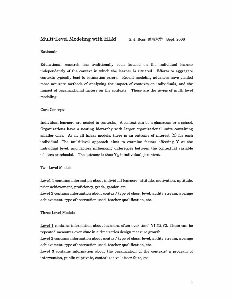
Two Level Models Step 1 Check Level 1 file structure. The key field should be left-most and indicate the nesting structure at level 1. Here, ‘sect’ (classes) are the larger nested unit..

In the Level 1 file, variables of interest at the individual student level are held. The left-most variable ‘sect’ indicates that the first 15 students are nested in Class 1.

Three individual difference variables are listed for each student: gender, previous

achievement (GPA) and initial proficiency (TOEFL). These may serve as covariates or as moderators for the outcomes of interest.

The right-most variables Fscor1 and Fscor2 are ‘factor scores’ for each individual

student indicating his or her own tendency to agree with a 10 item survey about the usefulness and validity of PEER ASSESSMENT. These serve as the two dependent variables in the multi-level analysis.

3

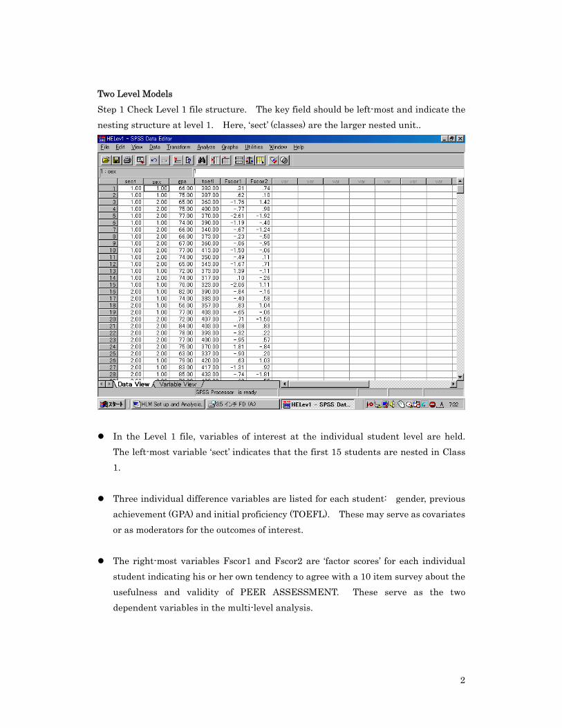
Step 2: Check Level 2 file structure. The left-most field should be the key variable for nesting at both Level 1 and Level 2. Here ‘Sect’ indicates classes. Fac1 and Fac2 are class averages for the PEER ASSESSMENT attitude survey. COHORT refers to those classes experiencing a PA training module vs classes that did not experience one.

Level 2 variables describe features of the sections (classes), not the individuals nested within the classes. These can be dummy codes (e.g. cohort identifier), or can be averages for the class variables (e.g. SES, Proficiency, Motivation, etc). They should define the ‘context’ in which individuals are nested.

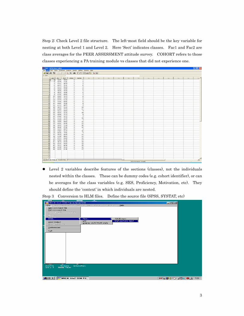
Step 3 Conversion to HLM files. Define the source file (SPSS, SYSTAT, etc)

4

Step 4 Locate data sets

Step 5. Browse Level 1 file first and identify the key field. Specify variables for analysis.

5

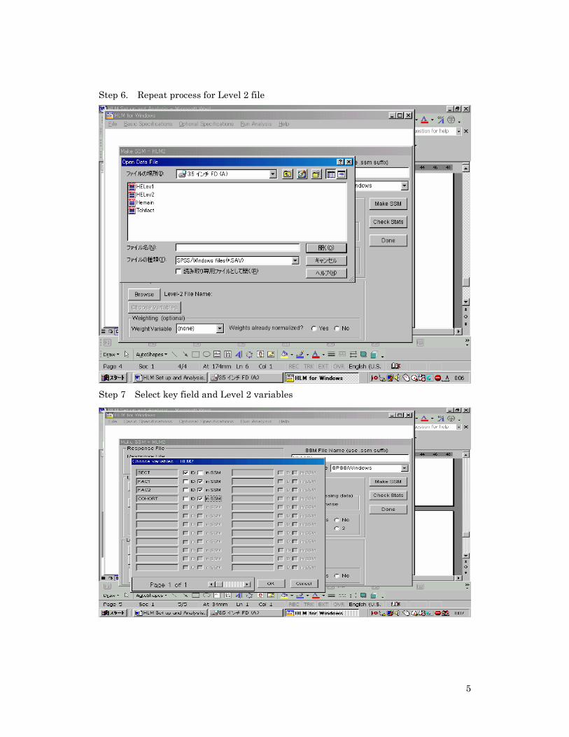
Step 6. Repeat process for Level 2 file

Step 7 Select key field and Level 2 variables

6

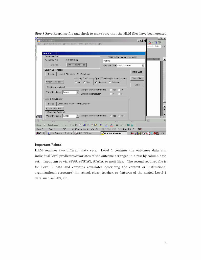
Step 8 Save Response file and check to make sure that the HLM files have been created

Important Points: HLM requires two different data sets. Level 1 contains the outcomes data and individual level predictors/covariates of the outcome arranged in a row by column data set. Input can be via SPSS, SYSTAT, STATA, or ascii files. The second required file is for Level 2 data and contains covariates describing the context or institutional organizational structure: the school, class, teacher, or features of the nested Level 1 data such as SES, etc.

7

HLM Analysis. Example 1. Learner attitudes toward peer assessment are the object of interest. A survey is given to 569 undergraduates who recently experienced peer assessment. Students are nested in 39 classes. Teachers are assigned multiple class sections. Can learner attitudes towards peer assessment be influenced by ‘innovation training’? In a contiguous cohort design, one cohort of learners does formative assessment over an academic year. The following year, another cohort does formative assessment, but receives modules designed to instruct the learners on how to do fair and accurate peer assessment. Does innovation training help? Survey Factorial Structure

Factor Loadings Plot

-1.0 -0.5 0.0 0.5 1.0FACTOR(1)

-1.0

-0.5

0.0

0.5

1.0

FAC

TOR

(2)

CLAR

EASY

HONEST

SIM

MOTDEEP

MORE

UNDER

Factor 1 members: More PA is needed, PA is motivating, PA gives deep assessments, PA gives learners better understanding. Factor 2 members: PA are honest, PA instructions are clear, PA is easy to do, PA is simple to implement. High scores imply agreement.

8

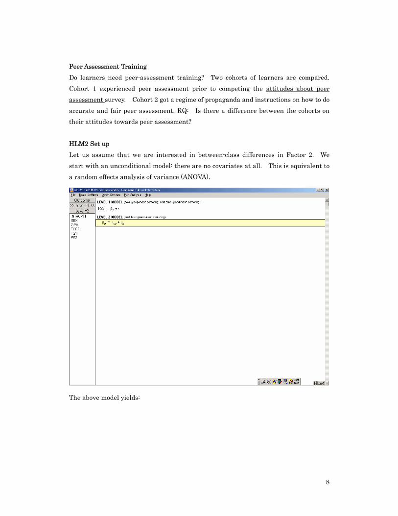
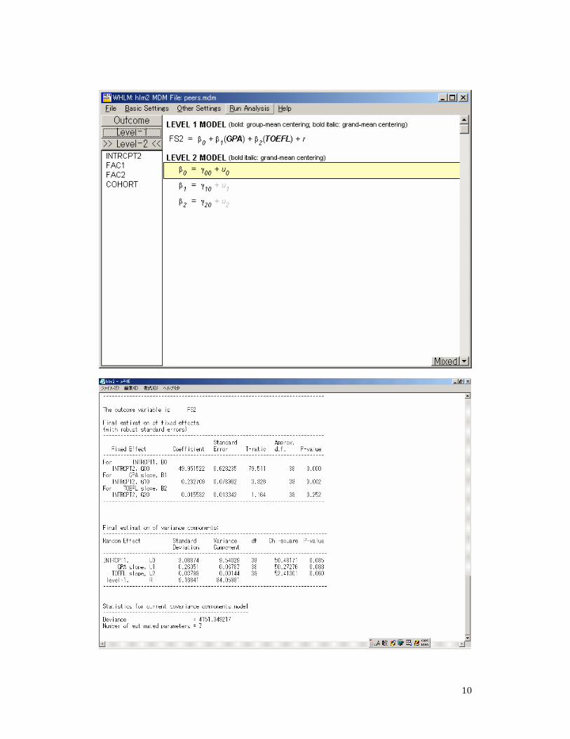
Peer Assessment Training Do learners need peer-assessment training? Two cohorts of learners are compared. Cohort 1 experienced peer assessment prior to competing the attitudes about peer assessment survey. Cohort 2 got a regime of propaganda and instructions on how to do accurate and fair peer assessment. RQ: Is there a difference between the cohorts on their attitudes towards peer assessment? HLM2 Set up Let us assume that we are interested in between-class differences in Factor 2. We start with an unconditional model: there are no covariates at all. This is equivalent to a random effects analysis of variance (ANOVA).

The above model yields:

9

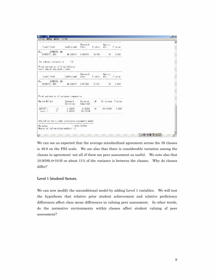
We can see as expected that the average standardized agreement across the 39 classes is 49.8 on the FS2 scale. We see also that there is considerable variation among the classes in agreement: not all of them see peer assessment as useful. We note also that 10.9/(89.4+10.9) or about 11% of the variance is between the classes. Why do classes differ? Level 1 (student) factors. We can now modify the unconditional model by adding Level 1 variables. We will test the hypothesis that relative prior student achievement and relative proficiency differences affect class mean differences in valuing peer assessment. In other words, do the normative environments within classes affect student valuing of peer assessment?

10

11

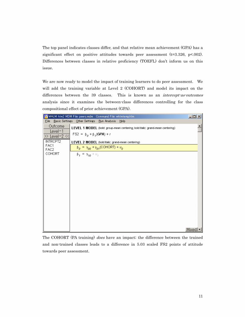
The top panel indicates classes differ, and that relative mean achievement (GPA) has a significant effect on positive attitudes towards peer assessment (t=3.326, p<.002). Differences between classes in relative proficiency (TOEFL) don’t inform us on this issue. We are now ready to model the impact of training learners to do peer assessment. We will add the training variable at Level 2 (COHORT) and model its impact on the differences between the 39 classes. This is known as an intercept-as-outcomes analysis since it examines the between-class differences controlling for the class compositional effect of prior achievement (GPA).

The COHORT (PA training) does have an impact; the difference between the trained and non-trained classes leads to a difference in 5.03 scaled FS2 points of attitude towards peer assessment.

12

We now turn to a related question. How does PA training moderate (interact with) the average achievement effect (GPA)? Does training have a differential affect for relative high and low achievers? Each class’s relative mean achievement (centered GPA) is the Level 1 covariate. The object of interest is whether the training in peer assessment moderates the effect of prior achievement (GPA) in each student’s attitude toward peer assessment. Here we focus on the slopes as outcome model.

13

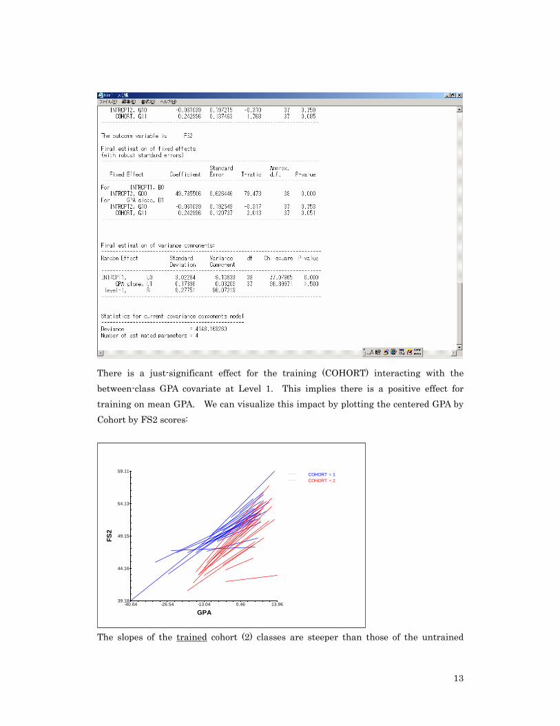
There is a just-significant effect for the training (COHORT) interacting with the between-class GPA covariate at Level 1. This implies there is a positive effect for training on mean GPA. We can visualize this impact by plotting the centered GPA by Cohort by FS2 scores:

-40.04 -26.54 -13.04 0.46 13.9639.18

44.16

49.15

54.13

59.11

GPA

FS2

COHORT = 1COHORT = 2

The slopes of the trained cohort (2) classes are steeper than those of the untrained

14

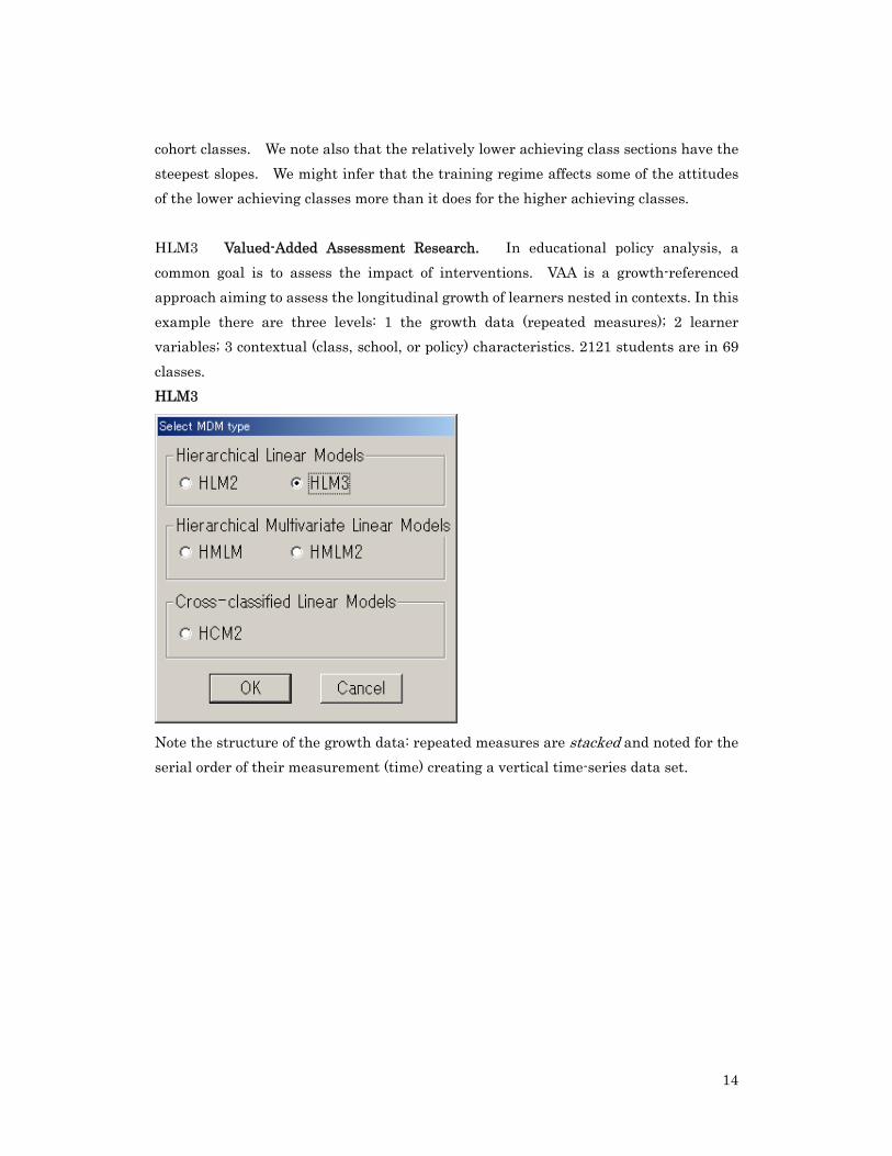
cohort classes. We note also that the relatively lower achieving class sections have the steepest slopes. We might infer that the training regime affects some of the attitudes of the lower achieving classes more than it does for the higher achieving classes. HLM3 Valued-Added Assessment Research. In educational policy analysis, a common goal is to assess the impact of interventions. VAA is a growth-referenced approach aiming to assess the longitudinal growth of learners nested in contexts. In this example there are three levels: 1 the growth data (repeated measures); 2 learner variables; 3 contextual (class, school, or policy) characteristics. 2121 students are in 69 classes. HLM3

Note the structure of the growth data: repeated measures are stacked and noted for the serial order of their measurement (time) creating a vertical time-series data set.

15

And locate the level 1 data set designed here as an SPSS file

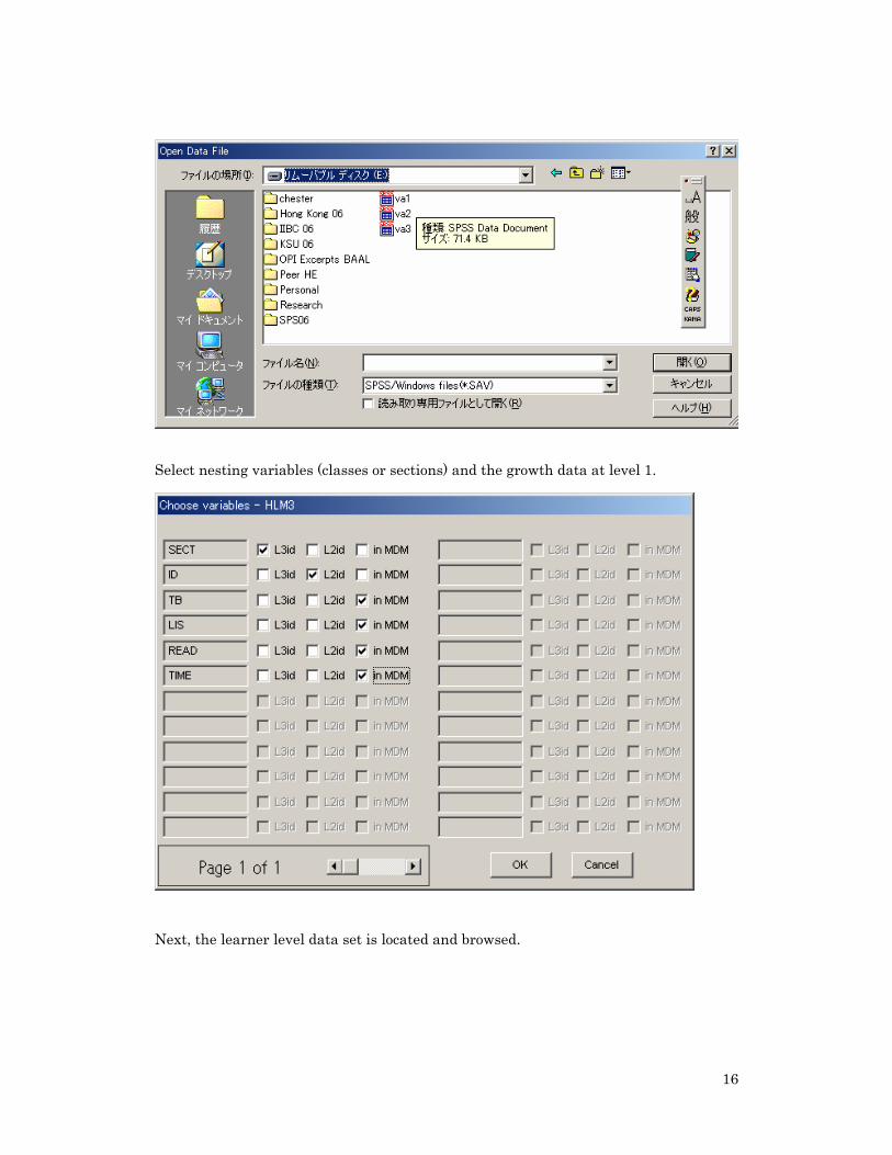
16

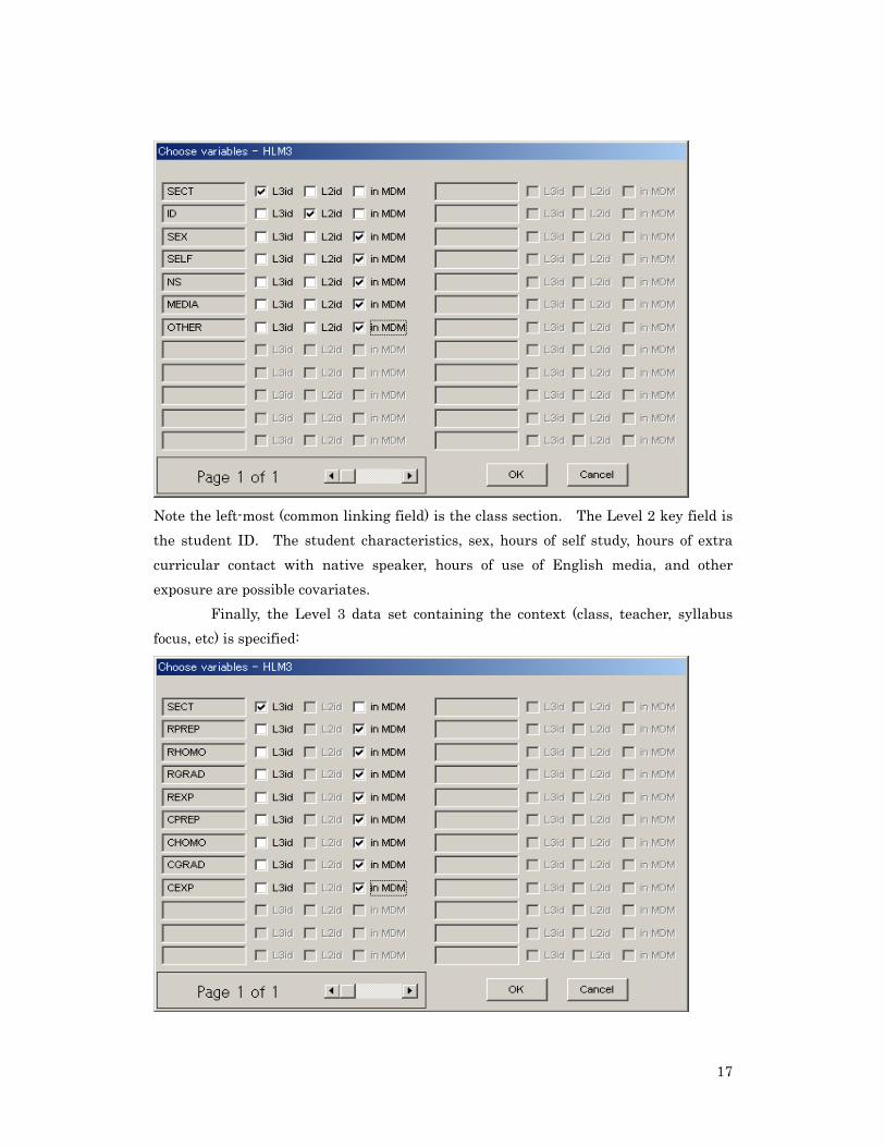
Select nesting variables (classes or sections) and the growth data at level 1.

Next, the learner level data set is located and browsed.

17

Note the left-most (common linking field) is the class section. The Level 2 key field is the student ID. The student characteristics, sex, hours of self study, hours of extra curricular contact with native speaker, hours of use of English media, and other exposure are possible covariates.

Finally, the Level 3 data set containing the context (class, teacher, syllabus focus, etc) is specified:

18

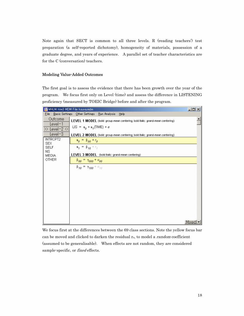
Note again that SECT is common to all three levels. R (reading teachers’) test preparation (a self-reported dichotomy), homogeneity of materials, possession of a graduate degree, and years of experience. A parallel set of teacher characteristics are for the C (conversation) teachers. Modeling Value-Added Outcomes The first goal is to assess the evidence that there has been growth over the year of the program. We focus first only on Level (time) and assess the difference in LISTENING proficiency (measured by TOEIC Bridge) before and after the program.

We focus first at the differences between the 69 class sections. Note the yellow focus bar can be moved and clicked to darken the residual ro, to model a random coefficient (assumed to be generalisable). When effects are not random, they are considered sample-specific, or fixed effects.

19

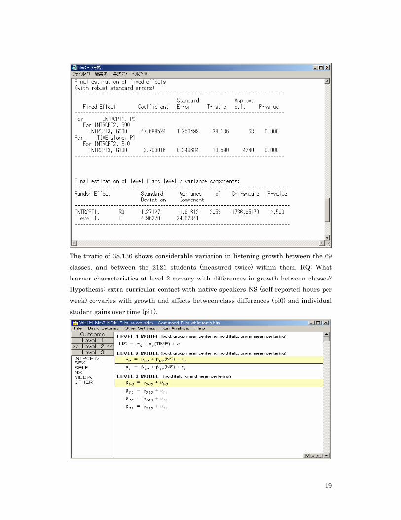
The t-ratio of 38.136 shows considerable variation in listening growth between the 69 classes, and between the 2121 students (measured twice) within them. RQ: What learner characteristics at level 2 co-vary with differences in growth between classes? Hypothesis: extra curricular contact with native speakers NS (self-reported hours per week) co-varies with growth and affects between-class differences (pi0) and individual student gains over time (pi1).

20

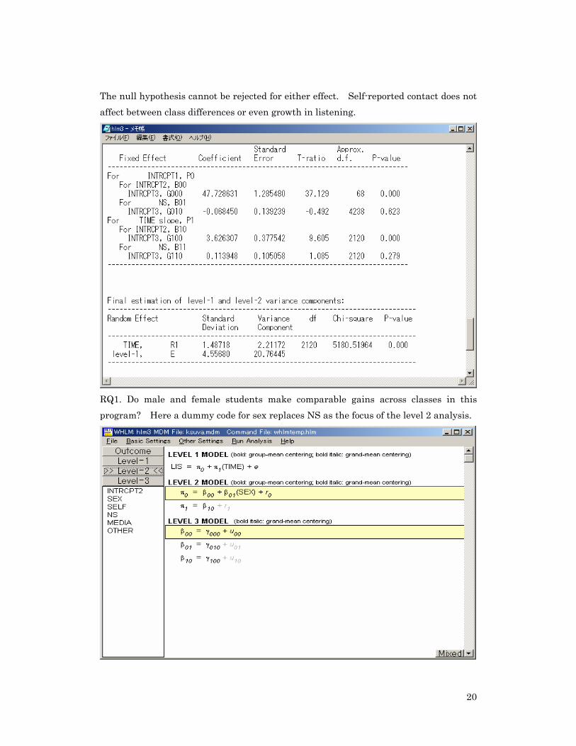
The null hypothesis cannot be rejected for either effect. Self-reported contact does not affect between class differences or even growth in listening.

RQ1. Do male and female students make comparable gains across classes in this program? Here a dummy code for sex replaces NS as the focus of the level 2 analysis.

21

The t-ratio of 2.78 indicates p<.006 that there is a gender difference influencing the difference between the class sections. Level 3 Analysis: What is the moderating influence of teachers’ decision to focus on test-prep on the gains in listening between class sections?

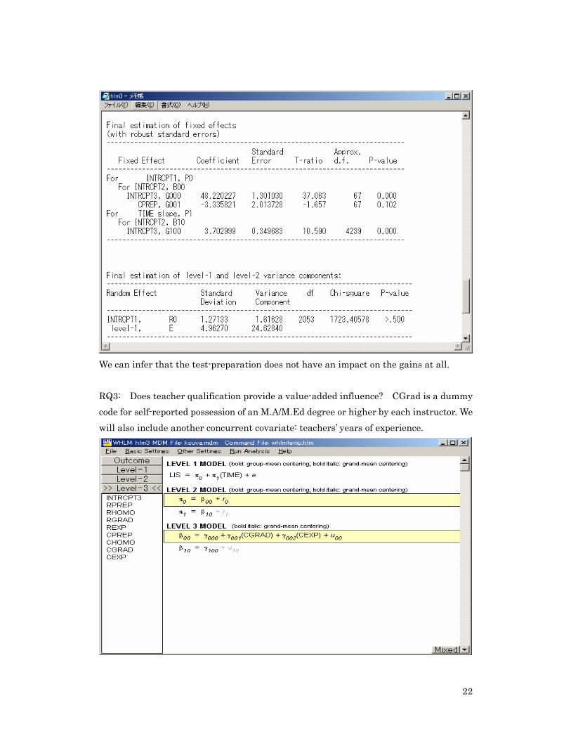
22

We can infer that the test-preparation does not have an impact on the gains at all. RQ3: Does teacher qualification provide a value-added influence? CGrad is a dummy code for self-reported possession of an M.A/M.Ed degree or higher by each instructor. We will also include another concurrent covariate: teachers’ years of experience.

23

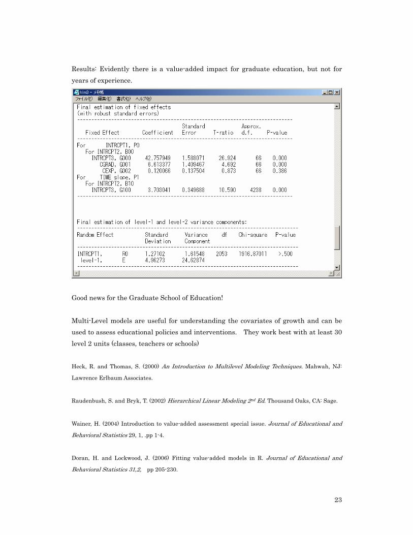
Results: Evidently there is a value-added impact for graduate education, but not for years of experience.

Good news for the Graduate School of Education! Multi-Level models are useful for understanding the covariates of growth and can be used to assess educational policies and interventions. They work best with at least 30 level 2 units (classes, teachers or schools) Heck, R. and Thomas, S. (2000) An Introduction to Multilevel Modeling Techniques. Mahwah, NJ:

Lawrence Erlbaum Associates.

Raudenbush, S. and Bryk, T. (2002) Hierarchical Linear Modeling 2nd Ed. Thousand Oaks, CA: Sage.

Wainer, H. (2004) Introduction to value-added assessment special issue. Journal of Educational and

Behavioral Statistics 29, 1, .pp 1-4.

Doran, H. and Lockwood, J. (2006) Fitting value-added models in R. Journal of Educational and

Behavioral Statistics 31,2, pp 205-230.

24