Embed Size (px)
Citation preview
University of Edinburgh
School of Informatics
Multiplication With Neurons
Author
Panagiotis E Nezis
Supervisor
Dr Mark van Rossum
Thesis
MSc in Informatics
August 17 2008
ἐν οἶδα ὁτι οὐδὲν οἶδαSocrates
ldquoI know that I donrsquot knowrdquo
Καὶ πάσχειν δή τι ὑπὸ τοῦ χρόνου καθάπερ καὶλέγειν εἰώθαμεν ὅτι κατατήκει ὁ χρόνος καὶ γηράσκει πάνθ᾿ὑπὸ τοῦ χρόνου καὶ ἐπιλανθάνεται διὰ τὸν χρόνον ἀλλ᾿ οὐ
μεμάθηκεν οὐδὲ νέον γέγονεν οὐδὲ καλόν φθορᾶς γὰρ αἴτιοςκαθ᾿ αὑτὸν μᾶλλον ὁ χρόνος ἀριθμὸς γὰρ κινήσεως ἡ δὲ
κίνησις ἐξίστησι τὸ ὑπάρχονAristotle
Physics Book IV Ch 12
A thing then will be affected by time just as we are accustomed to say that time wastes things awayand that all things grow old through time and that there is oblivion owing to the lapse of time
but we do not say the same of getting to know or of becoming young or fairFor time is by its nature the cause rather of decay
since it is the number of change and change removes what is
Translated from Greek by R P Hardie and R K Gaye
Abstract
Experimental evidence can be found that supports the existence of multiplicative mechanismsin the nervous system [23] The exact way multiplication is implemented in neurons is unclearHowever there is a lot of interest about its details driven by the experimental observationswhich imply its existence In this thesis we used feed forward networks of integrate-and-fireneurons in order to approximate multiplication The main hypothesis done is that the minimumfunction can give a multiplicative like response Networks that implement the minimum functionof two inputs were created and tested The results show that the hypothesis was correct andwe successfully managed to approach multiplication in most cases The limitations and someinteresting observations like the importance of spike timing are also described
i
ii
Acknowledgments
I would like to thank my supervisor Mark van Rossum for his enthusiasm encouragementand insight our discussions were as enjoyable as they were productive
I am also grateful to all other Professors I had both in the University of Edinburgh and theNational Technical University of Athens for turning me into a scientist
There is also a number of persons who may not have been directly involved in this projectbut without whom things would have been much harder
Last but not least my family receives my deepest gratitude and love for their faith and theirsupport during the current and previous studies
iii
iv
Declaration
I declare that this thesis was composed by myself that the work contained herein is my ownexcept where explicitly stated otherwise in the text and that this work has not been submittedfor any other degree or professional qualification except as specified
(Panagiotis Evangelou Nezis)
v
vi
Contents
Abstract i
Acknowledgments iii
Declaration v
1 Introduction 111 Proposal 112 Layout of the Thesis 2
2 Integrate-and-Fire Neuron Models 321 Introduction 322 Biological Background 4
221 Anatomy of a Neuron 4222 Membrane and Ion Channels 5223 Synapses 6
23 Electrical Properties of Cells 7231 Membrane Voltage - Resting Potential 7232 Spike Generation 7233 Membrane Capacitance amp Resistance 8234 Synaptic Reversal Potential and Conductance 8235 Electrical Structure of Neurons 9
24 The Integrate-and-Fire Model 9241 Nonleaky Integrate-and-Fire Neuron 9242 Leaky Integrate-and-Fire Neuron 10243 Synaptic Input 10
3 Multiplication in the Nervous System 1131 Introduction 1132 Importance of Multiplication 11
321 Function Approximation 11322 Relationship Between Operators 12323 Multiplication and Decision Making 12
33 Biological Evidence of Multiplication 13331 Barn Owlrsquos Auditory System 13332 The Lobula Giant Movement Detector LGMD of Locusts 14333 Other Evidence 16
34 Existing Models 17341 Multiplication via Silent Inhibition 17
vii
viii CONTENTS
342 Spike Coincidence Detector 17
4 Multiplication with Networks of IampF Neurons 2141 Introduction 2142 Aim of the Thesis 2143 Firing Rates and Rate Coding 21
431 Firing Rates 22432 Rate Coding 23
44 Excitation vs Inhibition 23441 Subtractive Effects of Inhibitory Synapses 24
45 Rectification 25451 Power-law Nonlinearities 27
46 Approximating Multiplication 2747 Proposed Networks 28
471 Network 1 29472 Network 2 29
5 Simulation Results 3151 Introduction 3152 Neuronrsquos Behavior 3153 Adjusting the Parameters 3354 Multiplication of Firing Rates 33
541 Experimental Procedure 33542 Experiment 1 34543 Experiment 2 36544 Experiment 3 36
55 Comparison of the Two Networks 3756 Spike Timing is Important 40
6 Discussion 4361 Introduction 4362 Achievements and Limitations 4363 Future Work 4364 Final Remarks 44
A Simulating Biological Neural Networks using SIMULINK 45A1 Introduction 45A2 SIMULINK 45
A21 Advantages of Simulink 45A22 S-functions 46
A3 The Biological Neural Networks SIMULINK Library (BNNSL) 49A31 Current Sources 49A32 Output Devices 49A33 Neuronal Models 49A34 BNNSL in Action 50
Bibliography 52
Chapter 1
Introduction
The way information is transmitted in the brain is a central problem in neuroscience Neuronsrespond to a certain stimulus by the generation of action potentials which are called spike trainsSpike trains are stochastic and repeated presentation of the same stimulus donrsquot cause identicalfiring patterns It is believed that information is encoded in the spatiotemporal pattern of thesetrains of action potentials There is a debate between those who support that information isembedded in temporal codes and researchers in favor of rate coding
In rate coding hypothesis one of the oldest ideas about neural coding [30] information isembedded in the mean firing rates of a population of neurons On the other hand temporalcoding relies on precise timing of action potentials and inter-spike intervals Aim of this proposalis to explore how networks of rate-coding neurons can do multiplication of signals
In the literature experimental evidence can be found that supports the existence of multiplica-tive mechanisms in the nervous system Studies have shown that the optomotor control in the flyis controlled by neural circuits performing multiplication [14][12] More recent experiments havefound a multiplicative like response in auditory neurons of the barn owlrsquos midbrain [23] [9]
The exact way multiplication is implemented in neurons is unclear However there is a lotof interest about its details driven by the experimental observations which imply its existenceKoch and Poggio [18] have discussed different biophysical properties present in single cells capableof producing multiplicative interactions In this proposal we are going to use integrate-and-fireneurons which donrsquot include the nonlinearities Koch and Poggio propose As a result the mainaim is to approximate multiplication being confined by the limits of these neuronal models
11 Proposal
In this project we are going to use feed-forward networks of integrate-and-fire neurons Theaim of these small population models is not to do exact multiplication since this is not possiblebut to approximate it Synaptic input is inserted in the neurons among with a noisy bias currentThe synapses may be either excitatory or inhibitory
An excitatory synapse is a synapse in which an action potential in the presynaptic cell increasesthe probability of an action potential occurring in the postsynaptic cell A postsynaptic potentialis considered inhibitory when the resulting change in membrane voltage makes it more difficult forthe cell to fire an action potential lowering the firing rate of the neuron They are the oppositeof excitatory postsynaptic potentials (EPSPs) which result from the flow of ions like sodium intothe cell
In our case inhibition is implemented through GABAA synapses with a reversal potentialequal to the resting one [30] This is called shunting inhibition and it has been shown to have asubtractive effect to the firing rate in most circumstances (the shunting conductance is independent
1
2 Chapter 1 - Introduction
of the firing rate) [16] despite its divisive effect in subthreshold amplitudesSince the firing rate of a neuron cannot take a negative value the output will be a rectified copy
of the input which is the difference between the excitatory and inhibitory synaptic inputs Theonly nonlinearity present in this neuronal model is the rectification We are going to combine itwith excitation and subtractive inhibition in order to approximate multiplication The minimumfunction is going to be used to approximate multiplication Boolean functions like minimum ormaximum can easily be implemented using rate coding neurons
12 Layout of the Thesis
The contents of this thesis are structured in such a way that the non-specialist reader ispresented initially with all the background knowledge needed The aim was to make the thesisas self-contained as possible Readers who are familiarised with the concepts presented in thebackground chapter could skip it or read it selectively
The remainder of this thesis is outlined as follows Chapter 2 presents all background knowl-edge needed in order a non-specialist reader to be able to understand the rest of this thesis Themain aim of this chapter is to present the Integrate-and-Fire neuron model but first the necessaryunderlying biological concepts are described We present the anatomy of a neuron we analyzethe electrical properties of neural cells and how action potential are generated before giving theequations that describe the Integrate-and-Fire model This chapter (or part of it) could be skippedby somebody familiar with this background information
In Chapter 3 we try to mention the importance of this thesis Initially we explain abstractlythe necessity of a multiplicative operation in perceptive tasks and describe its relation with theBoolean AND operation Next we present experimental evidence of multiplicative operations inthe neural system The fact that the mechanisms that implement such multiplicative operationsare not well researched despite there are multiple reports about neural multiplication mademe interested in this thesis Finally on the same chapter we present some of the models thatresearchers have proposed
In Chapter 4 we present our approach to the problem of multiplication like operations in thebrain Initially we show that an Integrate-and-Fire neuron with an excitatory and an inhibitoryinput acts as a rectifying unit Next we show that multiplication could be approached with theminimum function given that we donrsquot care for the exact multiplication of two firing rates butfor a proportional relation Finally we present two feed forward networks of IampF neurons thatimplement the minimum function and were used in the simulations
The results of our research can be seen in Chapter 5 The simple networks proposed inChapter 4 are able to implement multiplicative like operations however their performance is notthe same We show which of the two networks performs better and try to analyze why thishappens We also ldquoproverdquo another important fact that spike timing is important even whendealing just with rate coding networks Finally in Chapter 6 we discuss the results of this thesisand propose some things that could be done if time permitted it
In order to do the simulations we created a SIMULINK library specific for Integrate-and-Fireneurons The Appendix describes how SIMULINK works its advantages compared to otherapproaches the Library we created and some examples of its usage
Chapter 2
Integrate-and-Fire Neuron Models
21 Introduction
The nervous system which is responsible for every action we make has a magnificent structureincluding billions of neurons connected to each other in an intricate pattern [13] Neurons arethe elementary processing units in the brain and communicate with short electrical pulses knownas spikes or action potentials It is believed that information is transmitted through firingsequences of spikes Although spiking neurons are the majority of cells present in the cortex thereis also a large number of glia cells that play a supporting role and are responsible for energysupply of the brain In Figure 21 we can see coloured hippocampal neurons and glia cells
Figure 21 Left-Hippocampal neurons (green) and glial cells (red) Right- Hippocam-pal neuron expressing monomeric Green Fluorescent Protein (GFP) (Images taken fromhttpwwwgreenspineca)
Biological research has produced detailed knowledge about the biophysical mechanisms under-lying neuronal functionality and spike generation From a modeling perspective this knowledgecan be used in order to construct neuron models which can be used in computer simulations ofneurons and neural networks These simulations can help us understand how information is en-coded into neural signals and how the network connectivity determines the firing activity A largenumber of neuron models has been proposed ranging from complex realistic descriptions of the
3
4 Chapter 2 - Integrate-and-Fire Neuron Models
Figure 22 Diagram of a typical neuron (Image taken from Wikipedia)
biophysical mechanisms to simplified models involving a small number of differential equationsThese simplified models may seem unrealistic but are very useful for the study and analysis oflarge neural systems
In this chapter we are going to present the Integrate-and-Fire model one of the most widelyused neuron models which uses just one differential equation to describe the membrane potentialof a neuron in terms of the current it receives (injected current and synaptic inputs) This is themodel we are going to use for the multiplication networks in this thesis Before it we will describesome underlying biological concepts like the anatomy of neurons and the electrical properties ofthe membrane
22 Biological Background
Before describing the Integrate-and-Fire model it would be helpful to give some biologicalbackground about neurons and biological cells in general In this section the anatomy of neuronsis described along with the structure of cellular membranes the operation of ion channels whichare responsible for spike generation and finally the synapses and synaptic transmission
221 Anatomy of a Neuron
Neurons are electrically excitable cells in the nervous system that process and transmit infor-mation They are the most important units of the brain and of the whole nervous system There isa wide variety in the shape size and electrochemical properties of neurons which can be explainedby the diverse functions they perform
In Figure 22 we can see a diagram of the anatomy of a typical neuron The soma is thecentral part of the neuron where all the ldquocomputationalrdquo procedures like spike generation occur
Section 22 - Biological Background 5
Several branched tendrils are attached to neurons Each neuron has multiple dendrites whichplay a critical role in integrating synaptic inputs and in determining the extent to which actionpotentials are produced by the neuron
There is just one axon which is a long nerve fiber which can extend tens hundreds or eventens of thousands of times the diameter of the soma in length In contrast with dendrites theaxon conducts electrical impulses away from the neuronrsquos cell body acting as a transmission lineAction potentials almost always begin at the axon hillock (the part of the neuron where thesoma and the axon are connected) and travel down the axon
Finally synapses pass information from a presynaptic cell to a postsynaptic cell We will seesynapses and synaptic transmission in more detail in a following paragraph
222 Membrane and Ion Channels
The cell membrane is a selectively permeable lipid bilayer found in all cells It contains a widevariety of biological molecules mainly proteins and lipids which play a significant role for manycellular processes such as ion channel conductance and cell signaling
In Figure 23 we can see an illustration of the membrane The spherical lipid bilayer is ap-proximately 7 nm thick and is responsible for regulating the movement of materials into and outof cells Except the phospholipid bilayer we can see that the membrane includes several mem-brane proteins which determine the selective permeability of the membrane and passive and activetransport mechanisms
Figure 23 Illustration of a cell membrane We can see the phospholipid bilayer and some of theproteins lipids and other biological molecules that it contains Among these proteins we can see an ionchannel (Image taken from Wikipedia)
6 Chapter 2 - Integrate-and-Fire Neuron Models
The most important proteins for neural functionality are the ion channels integral membraneproteins through which ions can cross the membrane There are plenty such channels most ofthem being highly selective and allowing only a single type of ion to pass through them Thephospholipid bilayer is nearly impermeable to ions so these proteins are the elementary unitsunderlying principal functionalities such as spike generation and electrical signaling (within andbetween neurons)
223 Synapses
Synapses are specialized junctions responsible for the communication between neurons Thereare two main types of synapses the chemical ones and the electrical synapses which are also knownas gap-junctions [6] Chemical synapses are the most important and most numerous in the nervoussystem Despite gap junctions are very important parts of the nervous system (for example theyare particularly important in cardiac muscle [25]) in this thesis we will assume that only chemicalsynapses are present on the dendritic tree In the following paragraphs we will briefly describehow a synapse works
In chemical synapses transmission is mediated by a chemical called neuro-transmitter [31]Synaptic transmission begins when an action potential reaches the presynaptic axon terminalThe occurring depolarization of the presynaptic membrane initiates a sequence of events lead-ing to neurotransmitter release and activation of receptors on the postsynaptic membrane Anillustration of a synapse can be seen on Figure 24
Figure 24 Illustration of a synapse and synaptic transmission (Image taken from [21])
Axon terminal contains a ldquopoolrdquo of synaptic vesicles which are little balls filled with neuro-transmitter When the axon terminal is depolarized voltage-gated calcium (Ca) channels openand calcium ions (Ca2+) rush into the axon terminal Some of these ions bind to synaptic vesi-cles bringing them closer to the presynaptic membrane causing a fusion between the vesicle andsynaptic membrane and finally the neurotransmitter is released which goes into the extracellularspace
Some of the neurotransmitter molecules bind to special receptor molecules on the postsy-naptic membrane The response of the postsynaptic cell varies since it depends on the kind oftransmitter-receptor combination For excitatory synapses the neurotransmitter causes the open-ing of channels which let through ions of potassium K+ and Sodium Na+ On the other handinhibitory synapses activate mainly Chlorine channels Clminus
Section 23 - Electrical Properties of Cells 7
23 Electrical Properties of Cells
A neural cell can be modeled using electrical components like resistors capacitors and voltagesources The occurring electrical circuits are used for computational simulations and approachsufficiently the behavior of real cells
231 Membrane Voltage - Resting Potential
If one measures the intracellular (Vi) and extracellular (Ve) potentials of a neuron one willobserve the existence of a voltage difference (Vm) across its membrane
Vm(t) = Vi(t) minus Ve(t) (21)
Different intracellular and extracellular concentrations of ions are responsible for this voltageMost of the times Vm is negative (except when a spike occurs)
If the neuron is in rest (the sum of ionic currents flowing it and out of the membrane is zero)then the electrical potential across the membrane is called resting potential Vrest For a typicalneuron Vrest is about minus70 mV
232 Spike Generation
Figure 25 Generation of an action potential
The uniqueness of neurons is their abilityto produce propagate and decode spike trainsBefore presenting the way a neural cell can berepresented electrically it would be interestingto see how a spike is generated
If we inject the neuron with current theVm increases When the membrane potentialreaches a certain threshold enough voltage-gated sodium channels open and the relativeionic permeability favors sodium (Na) overpotassium (K) The number of channels thatopen depends on the injected current andequivalently to the voltage applied at the mem-brane This explains why higher potentialcause faster spikes When the cell is in restthere is a negative electrical potential inside itThe opening of the channels makes the Na+
ions flow into the cell causing a rapid depolar-ization of the membrane The flow of positivecharged ions inside the cell leads the membraneto a potential close to ENa After it the volt-age gated sodium channels inactivate and thevoltage-gated potassium channels open As aresult K+ ions rush out of the cell through theopen channels causing the membrane potentialto become negative again Since at this timethere is very little sodium permeability the po-
tential approaches EK causing a hyperpolarization close to the resting potential until the potas-sium channels close again This is the process of a spike generation Sodium channels cannot beactivated again until some time has passed (this time is known as the absolute refractory period)
8 Chapter 2 - Integrate-and-Fire Neuron Models
233 Membrane Capacitance amp Resistance
Capacitance Cm
The neuron membrane as we have already seen is an insulating layer consisting mainly oflipids and proteins However both the intracellular and extracellular solutions contain ions andhave conducting properties So the role of the insulating membrane is ldquoequivalentrdquo to that of acapacitor on an electrical circuit
The actual membrane capacitance Cm is specified in terms of the specific capacitance per unitarea cm measured in units of Farad per square centimeter (Fcm2) If A is the area of a cell (incm2) then the actual capacitance Cm (in F ) is given by
Cm = cm middot A (22)
Cm is proportional to membrane area A so the bigger the neuron the larger its capacitance Giventhat the charge distributed on a surface is proportional to the capacitance (Q = CV ) we can seethat larger neurons have bigger amounts of ions (charge) distributed across their membranes Atypical value for the specific capacitance cm which was used in our simulations is 1 microFcm2
Resistance Rm
The ion channels allow the ionic current to flow through the cellrsquos membrane Since there is adifference between the membrane voltage Vm and the resting voltage Vrest of the cell we can modelthe current flow through the ionic channels with a simple resistance Rm
The actual membrane resistance Rm is specified in terms of the specific resistance (or resistivity)rm measured in units of ohms-square centimeter (Ω middot cm2) If A the area of a cell (in cm2) thenthe actual resistance Rm (measured in Ω) is given by
Rm =rm
A (23)
We can see that Rm is inversely proportional to membrane area A so big neurons are more leakythan smaller cells A typical value for the resistivity rm which was used in our simulations is20 kΩ middot cm2
234 Synaptic Reversal Potential and Conductance
An ionic reversal potential V revsyn is associated to every synapse At this potential there is no
net flux of ions through the ionic channel and the membrane potential across it is stabilized toV rev
syn [17] For an excitatory synapse the reversal potential is about 0 mV while for an inhibitoryone V rev
syn has a value close to the neuronrsquos resting potential (minus70 mV )
It has been experimentally observed that spiking activity on the presynaptic cell causes aconductance change in the membrane of the postsynaptic cell This synaptic conductance gsyn(t)depends on the presence of presynaptic action potentials and changes with time It increasesalmost instantly to a maximum value g0 and then subsides exponentially within a time period of5 ms This is the synaptic time constant τsyn
Although ionic channels and synaptic transmission is a highly nonlinear phenomenon the pres-ence of a synapse in a membrane clatch can be modeled satisfactory with the synaptic conductancegsyn(t) in series with the synapsersquos reversal potential V rev
syn
Section 24 - The Integrate-and-Fire Model 9
235 Electrical Structure of Neurons
Using the aforementioned electrical properties of neural cells we can describe the dynamicsof the membrane potential Vm(t) in response to the input current using a single RC circuit Theexistence of a chemical synapse can be modeled by adding the synaptic conductance gsyn(t) andthe reversal potential V rev
syn in parallel with the RC circuit
R
V
CI m
m
rest
inj Vm
(a) Simple RC circuit
R
V
Cm
m
rest
Vm
Vrev
gsyn
( t )
(b) With synapse
Figure 26 Equivalent electrical circuits of a simple neuron (a) and a neuron with a fast chemicalsynapse (b)
24 The Integrate-and-Fire Model
The Integrate-and-Fire (IampF) is a very simple neuron model used widely to simulate andanalyse neural systems [3] Despite its simplicity the IampF model captures key features of realneuronrsquos behaviour like the rapid spike generation The Integrate-and-Fire model emphasizes onthe subthreshold membrane voltage properties and doesnrsquot take into account complex mechanismsresponsible for spike generation like the ionic channels The exclusion of such difficult to modelbiophysical mechanisms makes the IF model capable of being analysed mathematically and idealfor simulations including large numbers of neurons Other neuron models like the Hodgkin-Huxleymodel [15] although they capture in a better way the biological mechanisms are too complex tobe used in computational simulations of larger networks For example the Hodgkin-Huxley modeldescribes both the subthreshold and the spiking behavior of membrane potential but is using fourcoupled differential equations
In 1907 Lapicque [19] introduced the IampF model which is a passive circuit consisting of aresistor and a capacitor in parallel which represent the leakage and capacitance of the membraneIn this simple model the capacitor is charged until a certain voltage threshold is reached At thispoint a spike occurs (the capacitor discharges) and the voltage is reset to a specific value (Vreset)There are two basic versions of the Integrate-and-Fire model which are described below
241 Nonleaky Integrate-and-Fire Neuron
The nonleaky (or perfect) IampF model includes only a single capacitance C which is chargeduntil a fixed and stationary voltage threshold Vthr is reached
This model doesnrsquot take into account the membrane resistance and as a result the leakingcurrent which makes it unphysiological However it is very simple to be described mathematicallyAssuming an input current I(t) the differential equation governing the voltage is
10 Chapter 2 - Integrate-and-Fire Neuron Models
CdV (t)
dt= I(t) (24)
When Vth is reached at time ti a spike δ(t minus ti) is triggered and voltage is reset to Vreset Fortref seconds following the spike generation any input is shunted to ground making another spikeduring the absolute refractory period impossible [17]
242 Leaky Integrate-and-Fire Neuron
In the more general leaky model the summed contributions to the membrane potential decaywith a characteristic time constant τm which is called the membrane time constant Again whenthe membrane voltage Vm reaches a fixed threshold Vthr an action potential is initiated After thespiking the voltage is reset to a resting value Vrest and the neuron is inactivated for a brief timecorresponding to the absolute refractory period
The model is described by the following differential equation
Cm
dVm(t)
dt= Ileak(t) + Inoise(t) + Iin(t) (25)
where Ileak(t) the current due to the passive leak of the membrane Inoise(t) the current due tonoise (0 for non noisy neurons) and Iin(t) the input current (injected through an electrode Iinj(t)andor through synaptic input Isyn(t)) So there are two components for Iin(t)
Iin(t) = Iinj(t) + Isyn(t) (26)
The leaking current is given by the equation
Ileak(t) = minus1
Rm
[Vm(t) minus Vrest] = minusCm
τm
[Vm(t) minus Vrest] (27)
where τm = RmCm the passive membrane time constant depending solely on membranersquos capac-itance Cm and leak resistance Rm For our simulations we used a membrane time constant ofτm = 20 ms
243 Synaptic Input
Although the study of neuronrsquos response to injected current pulses and noise is interesting froman experimental perspective it is not realistic In a real cell the main source of ldquoinput currentrdquo issynaptic input
Each neuron is synaptically connected to multiple other neurons through its dendrites Whenan external stimulus is presented to an organism (for example a visual stimulus) some cells activateand the generated spike trains propagate through the axons of the activated neurons acting asinputs to the cells connected on them
Assuming a presynaptic spike at time tspike the postsynaptic current Isyn(t) applied on theneuron at time t can be given by the following exponential equation describing an AMPA synapse
Isyn(t) = g(t)(
V revsyn minus Vm(t)
)
(28)
where the synaptic conductance g(t) is given by
g(t) = g0eminus
tminustspike
τsyn (29)
In the previous equations V revsyn is the synapsersquos reversal potential g0 the maximum synaptic
conductance and τsyn the synapsersquos time constant
Chapter 3
Multiplication in the Nervous System
31 Introduction
In the literature experimental evidence can be found that supports the existence of multiplica-tive mechanisms in the nervous system Studies have shown that the optomotor control in the flyis controlled by neural circuits performing multiplication [12] [14] More recent experiments havefound a multiplicative like response in auditory neurons of the barn owl rsquos midbrain [23]
The exact way multiplication is implemented in neurons is unclear However there is a lotof interest about its details driven by the experimental observations which imply its existenceKoch and Poggio [18] have discussed different biophysical properties present in single cells ca-pable of producing multiplicative interactions Also in the literature some other neuronal modelsimplementing multiplicative operations can be found (for example [27])
In this chapter we will initially try to show why multiplication is important and how it couldplay central role in decision making and perceptive tasks Following we present biological evidenceof multiplicative operation in the neural system and in the end we describe some of the modelsthat can be found in literature
32 Importance of Multiplication
The simplest neuron models operate under a regime of thresholding if the sum of all inputsexcitatory and inhibitory (inhibitory synapses have a negative weight while excitatory a positiveone) exceeds a certain threshold then the neuron is active otherwise there is no spike generationThis binary threshold function is the only nonlinearity present in the model In artificial neuralnetworks sigmoid functions are used to give a smoother input-output relationship
The threshold function may be the dominant nonlinearity present in neurons but it is notthe only one As we will see on the next section literature is full of experimental evidence thatsupports the presence of multiplicative operations in the nervous system Given that multiplicationis the simplest possible nonlinearity neuronal networks implementing multiplicative interactionscan process information [18]
Below we will try to show how powerful this simple operation is and we will highlight itsconnection with the logical AND operation We will also see how important multiplication is fordecision making tasks
321 Function Approximation
The Weierstrass approximation theorem states that every continuous function defined on aninterval [a b] can be uniformly approximated as closely as desired by a polynomial function More
11
12 Chapter 3 - Multiplication in the Nervous System
formally the theorem has the following statement
Theorem Suppose f is a continuous complex-valued function defined on the real interval [a b]For every ǫ gt 0 there exists a polynomial function p over C such that for all x in [a b] we have|f(x) minus p(x)| lt ǫ or equivalently the supremum norm ||f minus p|| lt ǫ
If f is real-valued the polynomial function can be taken over R
The only nonlinear operation present in the construction of a polynomial is multiplicationAs a result if neural networks are capable of doing multiplicative-like operators then they couldapproximate under weak conditions all smooth input-output transductions [18]
A polynomial can be expressed as the sum of a set of monominals A monominal of order kcan be modeled with a multiplicative neural unit which has k inputs
P (x) = a1 + b1x1 + b2x2 + c1x21 + c2x1x2 + (31)
322 Relationship Between Operators
In order to understand the importance of multiplication we should first understand that mul-tiplication is in fact a close relative of another far more fundamental operation the logical AND(and) operation In Boolean algebra x1 and and xi and xn is true only if xi is true for all i If thereexists some xi which is false then the whole expression is false This ldquobehaviorrdquo is similar to themultiplication with zero in classical algebra x middot 0 = 0 forallx isin R More strictly the behavior of theand operator is similar to the minimum function
On the other hand the second more common Boolean operation OR (or) can be parallelizedwith addition or more strictly with the maximum function On the following table we illustratethese relations in a truth-like table form
Relationship Between Operators
x y x and y x times y min(x y) x or y x + y max(x y)0 0 0 0 0 0 0 00 1 0 0 0 1 1 11 0 0 0 0 1 1 11 1 1 1 1 1 2 1
323 Multiplication and Decision Making
The parallelism between multiplication and the logical AND operation could explain the im-portance of multiplicative neural mechanisms from a decision making perspective Logical AND(and) operations are fundamental in such tasks and generally in the organization of perception Wewill try to demonstrate this importance with a simplified example
Imagine a bird whose diet includes an edible red flower In order to discriminate this flowerfrom another similar one our bird detects its characteristic odour So it eats only these red flowerswhich also have the desired smell This is nothing more than an AND based perceptive task
Assume that there are two regions in the birdrsquos neural system one responsible for recognisingthe red color and the other for recognising the desired odour The outputs of these neural regionsare combined in a third region which decides if a specific flower is edible or not If the two outputswere just added then a very strong output of the ldquocolor detectorrdquo would produce a stronger outputsignal than a modest output of both detectors That could lead the bird to eat a poisonous flowerIf on the other hand the outputs of the two detectors are multiplied then the performance wouldbe better The absence of one feature (color or odour) would suppress the output and prevent the
Section 33 - Biological Evidence of Multiplication 13
bird from classifying the flower as edible If on the other hand both features are present but weakthen the multiplicative operation would lead to a supra-linear enhancement of the output signal
Through this intuitive example we showed that perceptive tasks which include and operationscan modeled better using multiplication than simple addition However it is not known to whatextent multiplicative like mechanisms are present in the neural system In the next section wedo a literature research presenting evidence of such multiplicative behaviors However for binarysignals when imposing a threshold the difference between the AND operation and addition isminor
33 Biological Evidence of Multiplication
Multiplicative operations are thought to be important in sensory processing Despite theresearch on this topic is limited there is significant experimental evidence that reinforces the ideasfor multiplicative biophysical mechanisms The most interesting clue of multiplicative propertiesof neurons can be found in the auditory system There is also evidence that multiplication iscarried out in the nervous system for motion perception tasks [18] In the following sections wewill present these clues trying to underline the importance of multiplication
331 Barn Owlrsquos Auditory System
Barn owls are able to use their very accurate directional hearing to strike prey in completedarkness This impressive capability is based on a very complex auditory system barn owls havewhich among other specializations includes asymmetric external ears
As a consequence of this asymmetry the owlrsquos auditory system computes both interaural time(ITD) and level (ILD) differences in order to create a two dimensional map of auditory space [22]Interaural level differences (ILDs) vary with elevation allowing barn owls to use ILDs in orderto localize sounds in the vertical plane Similarly interaural time differences (ITDs) are used forlocalization in the horizontal plane
Neuronal sensitivity to these binaural cues first appears in the owls brainstem with separatenuclei responsible for processing ILDs and ITDs Both ITDs and ILDs information are mergedin space-specific neurons that respond maximally to sounds coming from a particular directionin space The parallel pathways that process this information merge in a region known as theexternal nucleus of the inferior colliculus (ICx) eventually leading to the construction of a neuralmap of auditory space (see Figure 31)
The research of Pena and Konishi [22] suggests that the space-specific neurons in the barnowl ICx tune at the location of an auditory stimulus by multiplying postsynaptic potentials tunedto ITD and ILD So the subthreshold responses of these neurons to ITD-ILD pairs have a multi-plicative rather than an additive behavior
Owls were anesthetized and postsynaptic potentials generated by ICx neurons in response todifferent combinations of ITDs and ILDs were recorded with the help of intracellular electroderecordings Acoustic stimuli were digitally synthesized with a personal computer and delivered toboth ears by calibrated earphone assemblies giving rise to the various ITD-ILD pairs [23] Theresearchers discovered that a model based on the product of the ITD and ILD inputs could accountfor more of the observed responses An additive model was also tested but it was not efficientand could not reconstruct the original data matrix as well as the multiplicative model In Figure32 we can see the success of the multiplicative model in reconstructing the measures membranepotential for different ITD-ILD pairs
14 Chapter 3 - Multiplication in the Nervous System
Figure 31 Space-specific neuron in barn owl rsquos auditory system that respond maximally to soundscoming from a particular direction in space (A) A drawing of an ICx neuron and its axon projectingto the optic tectum (OT ) (B) The same neuron labeled with neurobiotin (C) Postsynaptic potentialsin response to different ITD-ILD pairs Dotted lines indicate the mean resting potential (D) Spikingresponses of the same neuron to different ITD-ILD pairs The large peak is the excitatory center andthe flat area around it is the inhibitory surround [compare (C) and (D)] Negative (-)ITD and negative(-)ILD mean respectively sound in ipsilateral ear leading and louder (Figure and caption taken from[22])
332 The Lobula Giant Movement Detector LGMD of Locusts
Gabbiani et al [11] mention that there is evidence for the existence of a multiplicative operationin the processing of looming stimuli They experimented with a neuron in the locust visual system(the LGMD neuron) that responds well to objects looming on a collision course towards theanimal Multiplication could be used for the computation of an angular threshold that couldprevent collision with looming objects
The firing rate of the LGMD neuron was monitored by recording the action potentials of itspost-synaptic target neuron (DCMD) The insect was presented with black squares or disks on abright background which simulated approaching The monitored firing rate a firing rate initiallyincreased until a peak and finally it decayed as the approach ended
Section 33 - Biological Evidence of Multiplication 15
If we denote by l the looming object half-size by t the time to collision and by v its approachvelocity then the angular size is given by [10]
θ(t) = 2arctan
(
l
vt
)
(32)
In a beautiful analysis the researchers suggest that ldquothe angular threshold might be the image-based retinal variable used to trigger escape responses in the face of an impending collision Indeeda leg flexion (presumably in preparation for an escape jump) has been shown to follow the peakLGMD firing rate with a fixed delayrdquo [11]
The researchers tried to figure out how the the angular threshold is calculated by the insectrsquosnervous system They tried different models which were based on the size of the forthcomingobject and the velocity that could describe the recorded responses of the LGMD One input wasexcitatory and the other one inhibitory By using selective activation and inactivation of preand postsynaptic inhibition they found out that postsynaptic inhibition played a very importantrole suggesting that multiplication is implemented within the neuron itself [10] Experimentaland theoretical results are consistent with multiplication being implemented by subtraction oftwo logarithmic terms followed by exponentiation via active membrane conductances accordingtoa times 1
b= exp(ln(a) minus ln(b)) In Figure 33 we can see some of their results
Figure 32 Multiplicative combination of ILD and ITD inputs (A) Raw data matrix (B) Reconstruc-tion of the matrix from the computed left and right singular vectors and the first singular value Additionof V0 [DC offset (blue area)] that minimizes the second singular value almost restores the original matrix(C) ITD curve (D) ILD curve (E) Computed left singular vector (F) Computed right singular vector(Figure and caption taken from [22])
16 Chapter 3 - Multiplication in the Nervous System
Figure 33 Transformation between membrane potential (Vm) and firing rate at the spike initiationzone (a) Approaching stimulus (top) recordings from the DCMD (middle extracellular) and from theLGMD (bottom intracellular) close to its spike initiation zone (b inset) Orange trace is membranepotential after median filtering (V m) Inset bracketed portion of Vm and (V m) expanded 3 times (b)Top panel presents median filtered membrane potential (orange line is same trace as in a 5 repetitions)Bottom 5 traces were recorded after TTX application to the axon (inset) (c) Mean traces in control andTTX (from b) were fitted with a third-order polynomial (black) and used to compute the mean temporaldifference (352 ms) in membrane potential over the response rising phase (d) Fit of mean instantaneousfiring rate 〈g〉 as a function of mean median filtered membrane potential (mean plusmn sd solid and dottedblack lines) with linear third-power and exponential models (Figure and caption taken from [11])
333 Other Evidence
Multiplicative evidence can also be found in the optomotor control of the fly [12] [14] Theflyrsquos optomotor response to transient stimuli was studied under open loop conditions The stimuliused were moving edges and stripes A comparison of the flyrsquos responses to these stimuli led theresearchers to the result that progressive moving patterns elicit stronger responses (from front toback) than regressive moving ones (from back to front) The existence of such deviations in flyrsquosresponse to different moving edges suggests the evidence of nonlinearities in insectrsquos perceivingsystem
Section 34 - Existing Models 17
Research done by Reichardt [24] has also suggested that the optomotor response of insects tomoving stimuli is mediated by a correlation like operation which can be seen abstractly seen as aform of multiplication Similar experimental observations exist for pigeons as well [28]
Finally Andersen [1] reviews some research papers which indicate that ldquosensory signals frommany modalities converge in the posterior parietal cortex in order to code the spatial locationsof goals for movement These signals are combined using a specific gain mechanism rdquo
34 Existing Models
In the literature there are some papers which propose models for multiplicative neural oper-ations Most of these models are single cellrsquos specific biophysical mechanisms which could giverise to a multiplicative-like operation However we should note that the research in this field islimited despite the importance of understanding how multiplicative-like operations are neurallyimplemented In our proposal we wonrsquot concern with single cell models but with small feed for-ward networks of Integrate-and-Fire neurons On the following paragraphs we will briefly explainsome of the multiplicative models found in literature
341 Multiplication via Silent Inhibition
Silent inhibition in some special cases can give rise to a multiplicative behavior We have seenin the previous chapter that synaptic current is given by
Isyn(t) = gsyn(t)(
V revsyn minus Vm(t)
)
(33)
If we suppose that the synaptic input changes slowly [18] then we can assume that the synapticconductance gsyn(t) changes slowly with time As a result there will be a stationary current andgsyn will be the constant synaptic input If Rsyn the synaptic resistance then using Ohmrsquos lawV = R middot I we take the following equation for the membrane voltage
Vm =gsynRsynV rev
syn
1 + RsynV revsyn
(34)
If the synaptic reversal is close to the resting potential of the cell (shunting inhibition) then theaction of this synapse to Vm remains invisible
From the previous equation we can take a multiplicative relation if we assume that the productof the synaptic resistance and synaptic conductance is small gsynRsyn ≪ 1
Vm asymp gsynRsynV revsyn (35)
If we also have an excitatory synaptic input with an associated conductance change ge and areversal potential V rev
exc then using Taylor expansion we take [18]
Vm asymp V revexc Rsyn
(
ge minus g2e minus gegsynRsyn +
)
(36)
which includes quadratic contributions from the excitatory synaptic terms and higher order termsfrom combinations of the excitatory and inhibitory inputs
342 Spike Coincidence Detector
Srinivasan and Bernard [27] used an input spike coincidence detector in order to model mul-tiplication like responses The main aim of the authors was not to model exact multiplication
18 Chapter 3 - Multiplication in the Nervous System
but to describe a scheme by which a neuron can produce a response which is proportional to theproduct of the input signals that it receives from two other neurons
They investigated a neuronal model in which the neuron produces a spike only if it receivestwo spikes from the two external neurons that are coincident in time or nearly so In Figure 34we can see how such a neuron operates
Figure 34 Neuron C receives input from two neurons AB Cell C fires a spike only if two input actionpotentials arrive within a ∆ ms Only in this case the voltage membrane reaches the threshold As aresult the output firing rate of neuron C is proportional to the firing rates of AB (Figure taken from[27])
In order to model coincidence detection the proposed neuron spikes when its membrane voltageVm is above a certain threshold Vthr The presence of only one presynaptic spike cannot causeenough EPSP to discharge the cell but if two spikes arrive within ∆ ms then the voltage thresholdis reached and an output spike is generated If Vmax the maximum membrane potential theneuron can reach from a single input spike then there is an exponential decaying relation betweenmembrane voltage and time
V (t) = Vmaxeminus
tτ (37)
where τ the neuronrsquos time constant The authors make the assumption that Vmax lt Vthr lt 2Vmax
so a single spike cannot initiate a postsynaptic action potential If we have an input spike at timet0 there should be another spike in an interval of ∆ ms before (or after) t0 ([t0 minus ∆ t0 + ∆]) inorder to have the postsynaptic action potential Given two spikes at t and t + ∆ then the neuronwill fire an action potential and as a result ∆ can easily be determined by the equation
Vmaxeminus
∆
τ + Vmax = Vthr (38)
The authors assumed statistical independence of the two input firing rates (a natural assump-tion in most cases for example when the stimuli causing activation of the two presynaptic cells
Section 34 - Existing Models 19
are independent) and showed that the output firing rate is proportional to the product of the twoinput firing frequencies [27]
fout = 2∆fAfB (39)
20 Chapter 3 - Multiplication in the Nervous System
Chapter 4
Multiplication with Networks of IampFNeurons
41 Introduction
In the previous chapter we presented evidence of multiplicative behavior in neural cells Wealso argued for the importance of this simple nonlinear operation Despite its simplicity it isunclear how biological neural networks implement multiplication Also the research done in thisfield is limited and the models found in bibliography (we presented some of them in the previouschapter) are complex single cell biophysical mechanisms
We try to approach multiplication using very simple networks of Integrate-and-Fire neuronsand a combination of excitatory and inhibitory synapses In this chapter we are going to presentthe underlying theory and the proposed models We also analyze in depth the main idea behind thisdissertation which is the usage of the minimum function for implementing a neural multiplicativeoperator
42 Aim of the Thesis
The aim of this thesis is to find feed-forward networks of Integrate-and-Fire neurons which domultiplication of the input firing rates The problem can be defined as follows
ProblemGiven two firing rates ρ1 ρ2 [in Hz] find a network of Integrate-and-Fire neurons whose outputspike train has a firing rate ρout where
ρout = ρ1 middot ρ2 (41)
In the next sections we will see that the exact multiplication is not possible so we will try toapproximate it Before presenting the proposed networks we will give the definitions for firingrates and rate coding
43 Firing Rates and Rate Coding
The way information is transmitted in the brain is a central problem in neuroscience Neuronsrespond to a certain stimulus by the generation of action potentials which are called spike trainsSpike trains are stochastic and repeated presentation of the same stimulus donrsquot cause identicalfiring patterns It is believed that information is encoded in the spatiotemporal pattern of these
21
22 Chapter 4 - Multiplication with Networks of IampF Neurons
trains of action potentials There is a debate between those who support that information isembedded in temporal codes and researchers in favor of rate coding
In rate coding hypothesis one of the oldest ideas about neural coding [30] information isembedded in the mean firing rates of a population of neurons On the other hand temporalcoding relies on precise timing of action potentials and inter-spike intervals
431 Firing Rates
Suppose that we record the output of an integrate-and-fire neuron for a specific time intervalof duration T In total n spikes are observed which occur at times ti i = 1 n Then theneural response r(t) can be represented as a sum of Dirac functions
r(t) =n
sum
i=1
δ(t minus ti) (42)
The specific timing of each action potential is useful only if we use temporal coding In thisthesis we study the multiplication of firing rates so the times ti are not useful Due to theirstochastic nature neural responses can be characterized by firing rates instead of specific spiketrains [5]
Figure 41 Firing rates approximated by different procedures (A) A spike train from a neuron inthe inferotemporal cortex of a monkey recorded while that animal watched a video on a monitor underfree viewing conditions (B) Discrete time firing rate obtained by binning time and counting spikes for∆t = 100 ms (C) Approximate firing rate determined by sliding a rectangular window function along thespike train with ∆t = 100 ms (D) Approximate firing rate computed using a Gaussian window functionwith σt = 100 ms (E) Approximate firing rate using the window function w(τ) =
[
α2τ exp(minusατ)]
+
where 1α = 100 ms (Figure and caption taken from [5])
If there is low variability in the spiking activity then the firing rate can be accurately approachedby the spike count rate which is nothing more than the frequency if the n action potentials duringa time T
Section 44 - Excitation vs Inhibition 23
ρ =n
T=
1
T
int T
0
r(t)dt (43)
Of course if there is variability in the frequency of spikes this approximation is not sufficient anda time-dependent firing rate should be used The firing rate at time t in this case can be definedas the time of spikes between t and t + ∆t where ∆t a small time interval [5] So mathematicallywe can express ρ(t) as
ρ(t) =1
∆t
int t+∆t
t
〈r(t)〉dt (44)
where the trial averaged neural response 〈r(t)〉 is the sum of spike occurrences over the interval[t t + ∆t] for K trials divided by the number of trials K
432 Rate Coding
According to the rate coding hypothesis information is encoded in the mean firing rate of apopulation of neurons and not the exact timing of the action potentials It has been observedthat different stimuli cause spike trains of different frequencies on the same neurons Generallyas the intensity of a stimulus increases so does the frequency or rate of action potentials Theseexperimental observations have lead to the formation of rate coding hypothesis
Theunissen [29] defines rate coding as ldquoa coding scheme in which there is significant correlationbetween the relevant stimulus parameter and the mean number of spikes in the elicited responsewithin the encoding window and no additional correlation between the stimulus parameter andany higher-order moments (or higher-order principal components) of the elicited spike patternrdquo
Unlike rate coding [32] temporal coding relies on precise timing of action potentials or inter-spike intervals Combined with traditional rate coding models temporal coding can provideadditional information with the same rate There is strong evidence that temporal codes areused for cortical information transmission especially after the discovery of spike timing dependentplasticity [26]
Theunissen [29] defines temporal coding as ldquoa coding scheme in which there is significantadditional correlation between the relevant stimulus parameter and any moments of the elicitedspike pattern having higher order than the meanrdquo
44 Excitation vs Inhibition
We have seen in Chapter 2 that the main difference between an excitatory and an inhibitorysynapse is the reversal synaptic potential We are going to analyze on this section how the typeof the synapse affects the response of the cell for an input spike train
The synaptic current Isyn(t) is given by the following equation and depends on the synapticconductance g(t) and the difference between the reversal potential V rev
syn and the membrane voltageVm
Isyn(t) = g(t)(
V revsyn minus Vm(t)
)
(45)
where g(t) changes with time as we have already seen Let a time moment t0 where g(t0) = gt0 =50 pS For this time moment we plot the synaptic current for different values of the reversalpotential and the membrane voltage
For an inhibitory synapse the reversal synaptic potential is close to the resting potential ofthe neuron Vrest which in most cases is about minus70 mV On the other hand the reversal potentialfor an excitatory synapse is close to 0 mV In Figure 42 we can see that as V rev
syn increases sodoes Isyn For values of the reversal potential close to the ones observed on inhibitory synapses we
24 Chapter 4 - Multiplication with Networks of IampF Neurons
minus100minus80
minus60minus40
minus200
20
minus70
minus65
minus60
minus55
minus50minus3
minus2
minus1
0
1
2
3
4
x 10minus12
Reversal PotentialMembrane Voltage
Syn
aptic
Cur
rent
Figure 42 Plot of the synaptic current Isyn(t) for different values of the reversal synaptic potentialV rev
syn and the membrane voltage Vm The synaptic conductance was assumed constant to 50 pS
have negative synaptic current while a reversal potential of 0 mV can produce synaptic currentof about 3 pA
The positive synaptic current for an excitatory synapse has the following effect an actionpotential in the presynaptic cell increases the probability of an action potential occurring in thepostsynaptic cell On the other hand the minor synaptic currents caused by inhibitory synapsesresult in inconsiderable changes in the membrane voltage Vm and as a result to low firing possibili-ties Of course the existence of neural noise can cause the firing of a spike even if there is no inputcurrent In the case of both excitatory and inhibitory inputs on a neuron the negative inhibitorycurrent acts subtractively to the positive current of excitation In Figure 43 we can see how thefiring sequence of a neuron depends on the kind of the synapse for the same spike train input
Synapt ic Input
Cell Response
IampF
Excitatory
Inhibitory
Figure 43 Output spike train of an IampF neuron after stimulation with the sequence of action potentialpresented on the left We can see how the output depends on the kind of the synapse
441 Subtractive Effects of Inhibitory Synapses
A synapse is called inhibitory when its reversal potential is less than the threshold for actionpotential generation If it is close to the resting potential of the cell then this is called shuntinginhibition and has a divisive effect on subthreshold EPSP amplitudes [7]
However this divisive effect is not observed in firing rates Holt and Koch [16] have shownthat there is a subtractive effect on the firing rate This happens because the current that passes
Section 45 - Rectification 25
through the shunting conductance is independent of the firing rate The voltage at the shuntingsite cannot take a larger value than the spiking threshold and as a result the inhibitory synapticcurrent is limited for different firing rates Under these circumstances a linear subtractive operationis implemented
We simulated an Integrate-and-Fire neuron which had an excitatory and an inhibitory synapseThe reversal potential of the inhibitory one was close to the resting potential of the neuron makingit shunting On the following diagram we can see that there is indeed a subtractive effect on firingrates The firing rate of the spike train used as input to the excitatory synapse is 80 Hz whilethe inhibitory firing rates change from 0 to 80 Hz The firing rates of the output spike train areplotted among with the actual difference of the two input firing rates ρexc minus ρinh
0 10 20 30 40 50 60 70 800
20
40
60
80
100
120
Mean firing rate of the inhibitory input [in Hz]
Out
put f
iring
rat
e [in
Hz]
Figure 44 A noisy IampF neuron with two synaptic inputs (one excitatory and one inhibitory) wasstimulated and the output firing rates were recorded The firing rate of the excitatory input was keptconstant to 80 Hz while we were increasing the firing rate of the inhibitory input from 0 to 80 Hz witha step of 5 Hz With black circles we see the recorded output firing rates while the red triangles arethe difference between the excitatory and inhibitory firing rates ρexc minus ρinh We can see that there is asubtractive effect as expected
45 Rectification
Let an Integrate and Fire neuron (IampF) which is stimulated with excitatory presynaptic actionpotential whose average firing rate is ρexc
in and with inhibitory ones having a firing rate ρinhin The
output spike train depends on both the excitatory and inhibitory inputs and its firing rate is ρoutIf ρinh
in = 0 Hz then output firing rate will be close to the firing rate of the spike train arrivingat the excitatory synapse On the other hand the absence of excitatory input or the presenceonly of inhibitory presynaptic spikes will deter the neuron from spiking
26 Chapter 4 - Multiplication with Networks of IampF Neurons
If we have both excitatory and inhibitory synapses then as we have seen the inhibition has asubtractive effect on firing rates Since the firing rate of a neuron cannot take a negative valuethe output will be a rectified copy of the input
ρout = max(
0 ρexcin minus ρinh
in
)
=[
ρexcin minus ρinh
in
]
+(46)
where [middot]+ stands for rectification Since in our model we care only about firing rates (and notmembrane voltage dynamics) we should note that rectification will be the only present nonlinearityin the approximation of multiplication
A noisy integrate and fire neuron which has two synaptic inputs one excitatory and oneinhibitory was simulated for different values of ρexc
in and ρinhin The output firing rate ρout in all
cases was close to the rectified difference of the two inputs ρexcin minus ρinh
in as suggested by theory Theexpected output firing rates and the recorded ones are presented on the following figure for bothsimple rectification and power-law Nonlinearity
020
4060
80100
0
20
40
60
80
1000
20
40
60
80
100
Excitatory firing rates [in Hz]Inhibitory firing rates [in Hz]
Out
put f
iring
rat
es [i
n H
z]
(a) Recorded Firing Rates
020
4060
80100
0
20
40
60
80
1000
10
20
30
40
50
60
70
80
Excitatory firing rates [in Hz]Inhibitory firing rates [in Hz]
Out
put f
iring
rat
es [i
n H
z]
(b) Expected Firing Rates - Simple
020
4060
80100
0
20
40
60
80
1000
100
200
300
400
500
600
Excitatory firing rates [in Hz]Inhibitory firing rates [in Hz]
Out
put f
iring
rat
es [i
n H
z]
(c) Expected Firing Rates - Power Law
Figure 45 An IampF neuron with two synaptic inputs was simulated for different input firing rates inorder to examine if there is rectifying behavior Both the excitatory and inhibitory inputs ρexc
in ρinhin were
gradually increased from 5 to 90 Hz with a step of 5 Hz (a) Recorded output firing rates (b) Expectedinput-output relation according to the equation ρout =
[
ρexcin minus ρinh
in
]
+ (c) Expected input-output relation
according to the equation ρout =[
ρexcin minus ρinh
in
]145
+
Section 46 - Approximating Multiplication 27
We can see that the neuron responds as expected but there are some errors In Figure 46 weplot the error surface which is nothing more than the difference between the observed output firingrates and the expected ones The maximum error is 18 Hz and it was recorded for large firingrates of the excitatory input This is natural considering that for large excitatory input firingrates inter spike intervals are smaller than the synaptic time constant giving synaptic currentcapable of generating postsynaptic spikes This in combination with the noisy background currentcan explain this error of 20 Hz For smaller input firing rates the observed error is not more than5 Hz in most cases
020
4060
80100
0
20
40
60
80
100minus10
minus5
0
5
10
15
20
25
30
Excitatory firing rates [in Hz]Inhibitory firing rates [in Hz]
Err
or [i
n H
z]
(a) Error - Simple
020
4060
80100
0
20
40
60
80
100minus10
minus5
0
5
10
15
20
25
30
Excitatory firing rates [in Hz]Inhibitory firing rates [in Hz]
Err
or [i
n H
z]
(b) Error - Power Law
Figure 46 Error surfaces for a rectifying IampF neuron for different values of input firing rates Ifρexp the expected output firing rate and ρobs the observed one for two given values of input firing ratesρexc
in ρinhin then the error is defined as |ρobs minus ρexp| For both cases the error is similar
451 Power-law Nonlinearities
The approximation of multiplication using networks that do the minimum function can beimproved if the input-output relation is slightly nonlinear Generally a non-linear input-outputrelation of a rectifying neuron will have the form
ρout = ([
ρexcin minus ρinh
in
]
+)n (47)
where n is close to 1It can be found [30] that for n = 145 the error between the approximation and the exact
multiplication is minimum (see also Figure 47) Supra-linear relations of this kind have beenobserved in catrsquos visual cortex [2] Anderson et al compared the orientation tuning of spikes andmembrane potential responses in single cells They showed that noise can smooth the relationbetween membrane potential and spike rate since even subthreshold responses are capable ofgenerating spikes Miller and Troyer [20] extended Andersonrsquos work proving analytically that apower-law nonlinearity is the only input-output function that ldquoconverts contrast-invariant voltagetuning into contrast-invariant spiking tuningrdquo But the most important observation they made isthat addition of Gaussian noise to the cell causes a relationship between membrane voltage andfiring rate that is well approximated by an expansive power law
46 Approximating Multiplication
Ideally we want to find a network of Integrate and Fire neurons whose output is the product oftwo input firing rates ρ1 ρ2 But the exact multiplication is not possible since the only nonlinear
28 Chapter 4 - Multiplication with Networks of IampF Neurons
operator we have is the rectification So we will try to approach multiplication using the availablefunctionalities
Somebody would ask how we define the abstract term ldquoapproximation of multiplicationrdquo Whatwe actually want to approach is the output firing rates landscape Imagine that we have a firstpopulation of N neurons each responding with a specific firing rate fi 1 le i le N to a stimuluss1 and a second population of M neurons which respond with firing rates gj 1 le j le M to asecond stimulus s2 Consider a set of N timesM neurons arranged in a matrix form where the (i j)element is selective to the iminusth neuron of the first population and the jminusth neuron of the secondpopulation The output firing rates of these N timesM can be visualized as a three dimensional plotwhere the x and y axis correspond to the f g firing rates The z axis corresponds to the outputfiring rate of the set of N times M neurons
If the network approximates multiplication then the three dimensional plots should resembleto the landscape obtained if we multiplied every pair of fi gj and creating the corresponding plotSince exact multiplication is not possible in order to see how well a certain network approachesthe desired output we normalize the output firing rates and check which network minimizes theerror surface
The only ldquotoolsrdquo we have in order to construct networks performing a multiplication-like op-eration are excitation subtractive inhibition and rectification Multiplication is a close relative ofanother more fundamental operation the logical AND (and) Actually and is the binary equivalentof times Logical AND (like other logical operators) is fundamental in perceptive tasks and thatrsquosone more reason of the importance of multiplication Actually logical AND is nothing more thanthe minimum of the two binary digits So we could abstractly approach the multiplication of twofiring rates with the minimum of these two
HypothesisThe multiplication of two firing rates ρ1 ρ2 can be approached using the minimum function
ρ1 middot ρ2 asymp min (ρ1 ρ2) (48)
Actually multiplication is accurately approached using the minimum function [30] Usingrectifying neurons its very simple to create simple networks which theoretically have as output aspike train whose firing rate is the minimum of the two inputs ρ1 ρ2 For example
min (ρ1 ρ2) =[
ρ1 minus [ρ1 minus ρ2]+]
+
Let ρ1(x) = 4
1+eminusx and ρ2(y) = sin(y)+1 where x y take values from predefined intervals On thefollowing figure we can see the resemblance between the actual multiplication and the landscapeobtained using the minimum function If there exists a power law nonlinearity then the error isminimal
47 Proposed Networks
Since it is very easy to find networks of Integrate and Fire neurons that do Boolean operationslike the minimum function and given that multiplication can be approached accurately using theminimum we can restate our initial problem
ProblemGiven two firing rates ρ1 ρ2 [in Hz] find a network of Integrate-and-Fire neurons whose outputspike train has a firing rate ρout where
ρout = min (ρ1 ρ2) (49)
Section 47 - Proposed Networks 29
(a) Exact (b) Linear (c) Non-Linear
Figure 47 Multiplication of the firing rates ρ1(x) = 4
1+eminusx and ρ2(y) = sin(y) + 1 (a) Exact multi-plication (b) Approximation using the minimum function (c) Approximation if there is a supra-linearinput-output relation
In the following sections we are going to present two networks that find the minimum of thetwo input firing rates and were used for the simulations We should note that these networksare not unique and somebody could find many other networks that implement the same functionHowever their simplicity and the fact that they could easily be implemented computationallymade us select them Only feed forward connections are used despite computation could be alsoimplemented using feedback connections [30]
471 Network 1
The first proposed network can be seen in Figure 48 With arrows excitatory synapses arerepresented while circles stand for inhibitory synapses The minimum function is easily taken usingthe rectification function and a combination of excitatoryinhibitory synapses In this network alateral connection is used If f g the input firing rates then the firing rate of the output will bethe minimum of these two
The following rectifying function is implemented
min(f g) =[
f minus [f minus g]+
]
+(410)
472 Network 2
The second network (Figure 49) finds the double of the minimum using four integrate andfire neurons in a two layers feed forward neuron The rectifying function follows
2min(f g) =[
[f + g]+minus [f minus g]
+minus [g minus f ]
+
]
+(411)
30 Chapter 4 - Multiplication with Networks of IampF Neurons
g
fmin(fg)
if f gt g then f-g
else 0
if f gt g then f-(f-g) = g
else f-0 = f
Figure 48 A simple feed-forward network of IampF neurons which implements the minimum functionExcitatory synapses are represented as arrows while for inhibitory synapses circles are used
g
f
2min(fg)
if f gt g then f-g
else 0
f+g
if f gt g then 0
else g-f
if f gt g then f+g-(f-g)-0 = 2g
else f+g-0-(g-f) = 2f
Figure 49 A second feed-forward network of IampF neurons which implements the double of the minimumfunction Excitatory synapses are represented as arrows while for inhibitory synapses circles are used
Chapter 5
Simulation Results
51 Introduction
The networks presented in the previous chapter will be used for our simulations In this chapterwe are going to present the experimental results and discuss about the performance of the twonetworks We will see that in most cases our networks manage to approach multiplication
Before presenting the results we will show how we adjusted the parameters of the integrate-and-fire neurons in order to have the desired input-output relation Another very importantobservation we made and we will analyze in this chapter is the importance of spike timing Wewill see that the output of the networks does not depend only on the input firing rates but alsoon the exact timing of the spikes This may be a clue that temporal coding is also present inseemingly just rate coding functionalities Maybe the spatiotemporal pattern of the input spiketrains plays a minor role among with the crucial role of their firing rate
All computational simulations presented here were done using Simulink Simulink is an envi-ronment for multidomain simulation and Model-Based Design for dynamic and embedded systemsIt offers tight integration with the rest of the MATLAB environment and its usage is very simpleWe developed a library for the needs of our dissertation which can be used for simulations ofnetworks of Integrate-and-Fire neurons In the Appendix we present in detail this library
52 Neuronrsquos Behavior
Theoretically when an integrate-and-fire neuron has only one excitatory input then the firingrate of the output spike train should be equal to the input one But what happens in reality
We used Poisson spike generators to create spike trains with firing rates from 0 to 120 Hzwith a step of 5 Hz These spike trains were used as input at a noisy integrate-and-fire neuronwith the following parameters Vthr = minus50 mV Vrest minus 70 mV Vreset = minus70 mV τm = 20 msV exc
rev = 0 mV τsyn = 15 ms and g0 = 50 pS In order to have statistically correct results eachexperiment was repeated 100 times and the mean output firing rate was calculated
We plotted (Figure 51 a) the input-output firing rate relations Surprisingly we observe thatwhile for the first 40 Hz there is a linear relation for input firing rates greater than 40 Hz ρin 6= ρoutThe best fit is obtained with a cubic curve We can see that for the linear relation (red curve)significant errors are observed (Figure 51 b)
31
32 Chapter 5 - Simulation Results
0 20 40 60 80 100 120minus20
0
20
40
60
80
100
120
140
Input firing rate [in Hz]
Out
put f
iring
rat
e [in
Hz]
Data
Linear Fit
Cubic Fit
Quadratic Feet
(a)
0 20 40 60 80 100 120
minus10
minus5
0
5
10
Input firing rate [in Hz]
Err
or [i
n H
z]
linearquadraticcubic
(b)
Figure 51 (a) The input output relation for different input firing rates and polynomials (up to cu-bic) that fit this relation (b) Errors between the observed relation and the three polynomials Whiletheoretically there exists a linear relation we observe that a cubic curve approaches better the recordedinput-output firing rates
Section 53 - Adjusting the Parameters 33
53 Adjusting the Parameters
Before simulating the proposed networks we adjusted the parameters of the integrate and fireunits We remind that given an excitatory synaptic input with firing rate ρexc and an inhibitoryone with rate ρinh then the firing rate of the output spike train ρout should be
ρout = max (0 ρexc minus ρinh) = [ρexc minus ρinh]+
Given that parameters like the resting potential of the neuron or the threshold voltage areconstant and cannot be modified we will adjust the two parameters of the inhibitory synapse its reversal potential V inh
rev and the synaptic time constant τsynIn order to find the best pair
(
τsyn V inhrev
)
we used an error minimization criterion For twopredetermined input firing rates ρexc ρinh the absolute error between the expected output firingrate ρexpected
out and the observed one ρrecordedout is
error =| ρexpectedout minus ρrecorded
out | (51)
In order to take a more statistically accurate result we repeat the experiment with the samepair of parameters
(
τsyn V inhrev
)
P times and take the average error
error =
sumP
i=1| ρexpected
out minus ρrecordedout |
P=
sumP
i=1| [ρexc minus ρinh]+ minus ρrecorded
out |
P (52)
We varied the synaptic time constant τsyn from 5 to 25 ms and the reversal potential of theinhibitory synapse from minus100 to minus60 mV Both these value ranges are realistic and such parametervalues have been observed in biological neurons For every pair of parameters
(
τsyn V inhrev
)
wepresented the integrate and fire neuron with many different combinations of ρexc ρinh and averagedthe error Figure 52 is a plot of the mean error for different values of τsyn and V inh
rev We cansee that for τsyn = 15 ms and V inh
rev = minus90 mV the error is minimal These were the synapticparameters that were used in the simulations of the proposed networks
54 Multiplication of Firing Rates
Using the parameters that give the smallest error we simulated the two networks proposed inthe previous chapter In this Section we present the experimental results for different input firingrates All these experiments were conducted using the first proposed network (Figure 53-a) Inthe next section we will see that the second network has not so good performance The comparisonof the two architectures will be presented on a following section Before presenting the results wedescribe first the experimental procedure
541 Experimental Procedure
The input firing rates f g take values from two predefined vectors fvalues gvalues Let Nthe number of elements of vector fvalues and M the elements of gvalues Poisson spike generatorsare used to produce spike trains with the desired firing rates These vectors can be seen as apopulation response to a certain input
The simulation is run for every combination fvalues(i) gvalues(j) 1 le i le N 1 le j le M givingan array N timesM of output firing rates This can be seen as the output of a set of N timesM neuronswhere the (i j)th element is selective to the iminusth neuron of population ldquofrdquo and the jminusth neuronof population ldquogrdquo
34 Chapter 5 - Simulation Results
5
10
15
20
25
minus100
minus90
minus80
minus70
minus600
10
20
30
40
50
60
70
Synaptic time constant [in ms]V
rev [in mV]
Err
or [i
n H
z]
Figure 52 Mean Error (in Hz) for different pairs of synaptic time constant τsyn and reversal potentialof the inhibitory synapse V inh
rev For every pair of parameters an integrate-and-fire neuron was simulatedfor various inputs ρexc ρinh and the average error was taken We can see that for τsyn = 15 ms andV inh
rev = minus90 mV the error surface is minimized and the neuron ldquofitsrdquo better the desired rectifying behavior
542 Experiment 1
In this experiment two identical Gaussian like population responses are multiplied (Figure 54)There are 15 neurons in each population so 15times 15 output firing rates were recorded In order tounderstand better the results we make some three dimensional plots The x axis can be consideredas the number of neuron in population f while the y axis as the neuron in population g So forexample the (3 5) point in the xminus y plane corresponds to the neuron in the set of N timesM neuronsthat is selective to the third neuron of population f and the fifth one from population g Thecorresponding z axis value is the firing rate that was recorded
Three plots are created each time The lower left subplot (c) corresponds to the real multipli-cation of the two firing rate vectors
ρout(i j) = fvalues(i) middot gvalues(j) 1 le i le N and 1 le j le M (53)
Since Poisson spike generators are used there is a deviation between the mean firing rates asdefined in the two vectors and the spikes that are actually generated If f real
values(i) grealvalues(j) the
real input firing rates then on the upper right (b) plot we draw the expected result
ρout(i j) = min(
f realvalues(i) greal
values(j))
1 le i le N and 1 le j le M (54)
Finally on the lower right figure (d) we plot the firing rate that was recorded at the output ofthe network In order to evaluate the performance of the network this actual result (d) should becompared to the expected one (b)
Section 54 - Multiplication of Firing Rates 35
(a) Network 1 (b) Network 2
Figure 53 The two proposed networks that implement the minimum function
0 5 10 150
10
20
30
40
50
60
70
Neuron
Firi
ng R
ate
[in H
z]
(a) Firing Rates
0
5
10
15
0
5
10
150
10
20
30
40
50
60
70
f
Expected Result
g
(b) Expected Output
0
5
10
15
0
5
10
150
1
2
3
4
5
6
7
8
x 104
fg
(c) Exact Multiplication
0
5
10
15
0
5
10
150
5
10
15
20
25
30
35
40
45
f
Actual Result
g
(d) Recorded Output
Figure 54 Two identical Gaussian-like firing rates (a) are used to stimulate the network of Figure 53-a The exact multiplication (c) the expected one according to the recorded Poisson generatorsrsquo outputfiring rates (b) and the recorded firing rates at the output of the network (d) are plotted
36 Chapter 5 - Simulation Results
543 Experiment 2
A Gaussian like population response f (red curve on Figure 55-a ) and a two peak sinusoidallike population response g (blue curve on Figure 55-a ) was used as inputs On Figure 55 wecan see the expected and recorded outputs Once again the network performs a multiplicative likeoperation
0 2 4 6 8 10 12 14 160
10
20
30
40
50
60
70
80
90
Neuron
Firi
ng R
ate
[in H
z]
(a) Firing Rates
0
5
10
15
0
5
10
15
200
10
20
30
40
50
60
70
Neuron (f)
Expected Result
Neuron (g)F
iring
Rat
e [in
Hz]
(b) Expected Output
0
5
10
15
0
5
10
15
200
1000
2000
3000
4000
5000
6000
7000
8000
Neuron (f)
Multiplication
Neuron (g)
Firi
ng R
ate
[in H
z]
(c) Exact Multiplication
0
5
10
15
0
5
10
15
200
10
20
30
40
50
60
Neuron (f)
Network Output
Neuron (g)
Firi
ng R
ate
[in H
z]
(d) Recorded Output
Figure 55 The population responses f (red trace) g (blue trace) plotted in (a) are used to stimulatethe network of Figure 53-a The exact multiplication (c) the expected one according to the recordedPoisson generatorsrsquo output firing rates (b) and the recorded firing rates at the output of the network (d)are plotted
544 Experiment 3
Now we will examine if under some circumstances the network doesnrsquot have the desired be-havior Actually itrsquos a case were the minimum function doesnrsquot approach multiplication Imaginethat one of the two input population responses (for example f) is constant to some value c whichis smaller than any value in the other population response (g) Then while a multiplicative opera-tion would be a proportional projection of the g population response on the x axis correspondingto the neurons of population f the minimum gives always the value c So theoretically if gi thefiring rates of population g where gj gt c forallj min(gj c) = c while gj middot c sim gj So theoretically wetake a horizontal plane of height c instead of the desired projection
Section 55 - Comparison of the Two Networks 37
This is demonstrated with an example All g firing rates are 5 Hz while the population responseg is a Gaussian with a minimum firing rate of 10 Hz (Figure 56-a) We can see how different is theobserved output than the desired result (c) Even in this case network implements multiplicationand the recorded output firing rates are similar to the expected ones (compare subplots b and d)
0 2 4 6 8 10 12 140
10
20
30
40
50
60
70
80
Neuron
Firi
ng R
ate
[in H
z]
(a) Firing Rates
02
46
810
1214
0
2
4
6
8
100
2
4
6
8
10
12
Neuron (f)
Expected Result
Neuron (g)
Firi
ng R
ate
[in H
z](b) Expected Output
02
46
810
1214
0
2
4
6
8
1050
100
150
200
250
300
350
400
Neuron (f)
Multiplication
Neuron (g)
Firi
ng R
ate
[in H
z]
(c) Exact Multiplication
02
46
810
1214
0
2
4
6
8
102
4
6
8
10
12
14
16
Neuron (f)
Network Output
Neuron (g)
Firi
ng R
ate
[in H
z]
(d) Recorded Output
Figure 56 The population responses f (red trace) g (blue trace) plotted in (a) are used to stimulatethe network of Figure 53-a The exact multiplication (c) the expected one according to the recordedPoisson generatorsrsquo output firing rates (b) and the recorded firing rates at the output of the network (d)are plotted While the network finds the minimum between the two input firing rates in such an extremecase the minimum function is not able to approach the actual multiplication
55 Comparison of the Two Networks
The first network as we have seen gives accurate results according to the ones expected Onthe other hand the second network didnrsquot manage to approach multiplication so well We willnow present some examples trying to explain the different behavior of the two networks despitetheoretically they should both have similar results
In Figure 57 we see the network outputs of the two networks when both stimulated withthe same Gaussian-like firing rates of Figure 54 a On the left column we can see the output of
38 Chapter 5 - Simulation Results
Network 1 and the expected output (a and c respectively) while on the right column the respectiveplots for Network 2 are presented
0
5
10
15
0
5
10
150
5
10
15
20
25
30
35
40
45
f
Actual Result
g
(a) Network 1 - Recorded Output
0
5
10
15
0
5
10
150
10
20
30
40
50
60
70
Neuron (f)
Network Output
Neuron (g)
Firi
ng R
ate
[in H
z]
(b) Network 2 - Recorded Output
0
5
10
15
0
5
10
150
10
20
30
40
50
60
70
f
Expected Result
g
(c) Network 1 - Expected Output
0
5
10
15
0
5
10
150
20
40
60
80
100
120
140
Neuron (f)
Expected Result
Neuron (g)
Firi
ng R
ate
[in H
z]
(d) Network 2 - Expected Output
Figure 57 The population responses f (red trace) g (blue trace) plotted in 54 (a) are used to stimulatethe networks of Figure 53 We can see the recorded and expected outputs for both network architecturesIt is obvious that the first network has a better performance
In order to verify the better performance we conducted the same experiment but this time theinput firing rates were these plotted on Figure 55-a Again (Figure 58) we discover that Network1 has a much better performance
The reason for this difference in the experimental results between the two architectures can bejustified from the fact that the second network doesnrsquot return the minimum but twice the minimumAs we observe in both experiments for small expected firing rates (lt 70 Hz) the second networkhas the desired performance But for larger expected output firing rates this is not the case Thiscan be explained from the single neuronrsquos behavior Remember from the second Section of thischapter (Figure 51) that for large input firing rates there is no linear relation between input andoutput
Suppose that we have as inputs a firing rate f = 80 Hz and a firing rate g = 70 Hz Theoret-ically we would expect an output firing rate of ρout = 2 min(80 70) = 140 Hz This means that atotal firing rate of 140 Hz is the input of the output neuron of the second Network (ρe
inxcminus ρinhin )
Due to the nonlinear relation between input and output such a large input firing rate will not be
Section 55 - Comparison of the Two Networks 39
0
5
10
15
0
5
10
15
200
10
20
30
40
50
60
Neuron (f)
Network Output
Neuron (g)
Firi
ng R
ate
[in H
z]
(a) Network 1 - Recorded Output
0
5
10
15
0
5
10
15
200
10
20
30
40
50
60
70
80
Neuron (f)
Network Output
Neuron (g)
Firi
ng R
ate
[in H
z]
(b) Network 2 - Recorded Output
0
5
10
15
0
5
10
15
200
10
20
30
40
50
60
70
Neuron (f)
Expected Result
Neuron (g)
Firi
ng R
ate
[in H
z]
(c) Network 1 - Expected Output
0
5
10
15
0
5
10
15
200
50
100
150
Neuron (f)
Expected Result
Neuron (g)
Firi
ng R
ate
[in H
z]
(d) Network 2 - Expected Output
Figure 58 The population responses f (red trace) g (blue trace) plotted in 55 (a) are used to stimulatethe networks of Figure 53 We can see the recorded and expected outputs for both network architecturesIt is obvious that the first network has a better performance
40 Chapter 5 - Simulation Results
able to produce a spike train with firing rate greater than 100 Hz This combined with the neuralnoise and the losses of the previous layers among with the refractory period of the integrate-and-fire neurons are the reasons for this output
56 Spike Timing is Important
We will now examine how spike timing affects the behavior and the performance of our net-works Our models are based in the rectifying hypothesis The output of an integrate-and-fire neu-ron (with excitatory and inhibitory synaptic inputs) has a firing rate which is max (0 ρexc minus ρinh)We have shown in the previous chapter that this hypothesis is correct and our neurons have thedesired behavior But this ldquocorrectnessrdquo depends solely on the stochasticity of the Poisson inputspike trains
Imagine a very simple scenario where an integrate and fire neuron is stimulated with anexcitatory synaptic input of 10 Hz and an inhibitory input of 50 Hz Theoretically no spikes willbe generated and the postsynaptic firing rate will be 0 Hz If we simulate the neuron for 1 s andall 10 excitatory input spikes appear in the first 100 ms while all 50 inhibitory ones in the last900 ms then about 10 spikes will be generated This happens because in the first 100 ms of thesimulation there is no inhibitory current to reduce the excitatory one As a result the excitatorypresynaptic spikes are able to ldquocauserdquo a postsynaptic spike firing
In order to verify the importance of spike timing we cannot use Poisson spike train as inputsdue to their stochasticity We decided to eliminate any stochasticity and randomness in order tocheck the effect spike timing has In order to do so we used spike generators with constant firingrates which fired at exact times Given a firing rate r and the time of the first spike tstart then wecan determine the inter-spike interval χ using
χ =1000
rms (55)
The first spike is fired at tstart and then a new spike is generated every χ ms
0
5
10
15
0
5
10
150
10
20
30
40
50
60
70
Neuron (f)
Expected Result
Neuron (g)
Firi
ng R
ate
[in H
z]
(a) Exact
0
5
10
15
0
5
10
150
20
40
60
80
100
Neuron (f)
Network Output
Neuron (g)
Firi
ng R
ate
[in H
z]
(b) Observed
Figure 59 Importance of spike timing An integrate-and-fire neuron was simulated for different inputand output firing rates The spike generators generate action potentials with predetermined inter-spikeintervals In Case 1 g spikes occur at least 10 ms before the f ones (tfstart = tgstart + 10) (a) Expectedoutput (b) Observed output We see that in this case the recorded output firing rates approach the desiredones
Section 56 - Spike Timing is Important 41
For our simulations we used the first network while the experimentation methodology is iden-tical to the one used in the previous Sections We managed to demonstrate with a very simpleexperiment that spike timing is crucial
Case 1
The second input g is activated 10 ms before the first one (tfstart = tgstart + 10) So for smallfiring rates g spikes occur at least 10 ms before the f spikes In this case the result approachedthe desired one as we can see in Figure 59
Case 2
The second input g is activated 20 ms before f (tfstart = tgstart + 20)) So for small firing ratesg spikes occur at least 20 ms before the f spikes In this case the output is does not approach thedesired one the network does not perform multiplication and there is substantial difference withthe result of Case 1 as we can see in Figure 510
0
5
10
15
0
5
10
150
10
20
30
40
50
60
70
Neuron (f)
Expected Result
Neuron (g)
Firi
ng R
ate
[in H
z]
(a) Exact
0
5
10
15
0
5
10
150
10
20
30
40
50
60
Neuron (f)
Network Output
Neuron (g)
Firi
ng R
ate
[in H
z]
(b) Observed
Figure 510 Importance of spike timing An integrate-and-fire neuron was simulated for different inputand output firing rates The spike generators generate action potentials with predetermined inter-spikeintervals In Case 2 g spikes occur at least 20 ms before the f ones (tfstart = tgstart + 20) (a) Expectedoutput (b) Observed output The importance of spike timing is obvious compared to Figure 59
Explanation
Why is spike timing so important and there is such difference between Case 1 and Case 2Remember that the synaptic time constant is 15 ms In the second case at the lower left neuronof the network (Figure 48) excitatory input spikes occur at least 20 ms after the inhibitory onesThe synaptic current is decaying exponentially and τsyn determines how fast it goes back to zeroafter a presynaptic spike So the synaptic current due to the inhibitory synapse has a very smallvalue 15 ms after the presynaptic inhibitory event which doesnrsquot manage to restrain the effect ofthe excitatory inputs As a result most of the time presynaptic spikes of the excitatory synapsemanage to raise the membrane voltage Vm above threshold and an action potential is generated
So neurons in this case have different behavior from the expected one and as a result the wholenetwork cannot perform multiplication as theory predicted Of course in real neurons spike trainsare stochastic and such an extreme case where there are determined inter-spike intervals are notrealistic
42 Chapter 5 - Simulation Results
Chapter 6
Discussion
61 Introduction
This chapter summarizes the project including its achievements and limitations and puts itin a wider context for review
62 Achievements and Limitations
The project was successful in achieving its outlined aims and objectives The proposed networksmanaged to approach multiplication This was shown through a series of experiments Howeverthe performance of the two networks was not the same (as expected) and also in some extremecases the result is not proportional to a multiplicative operator
We also showed that inhibition has a subtractive effect in rate codes under certain circum-stances This makes the proposed networks more realistic Compared to the other models formultiplication of neural signals found in the literature our two networks are very simple andstraight forward to understand
Finally one other achievement of this thesis was the development of the Biological NeuralNetworks Library for Simulink It is a tool that can be used for the simulation of any neuralnetwork while one can extend it by adding models of other cells
63 Future Work
If time permitted there are several issues that could be improved and more tests done Firstof all we could study in detail the importance of noise There is enough evidence that noise playsa crucial part in neural information processing and neural signals transmission Actually in thecortex of the brain noise is not just noise at all but contains information reflecting the activityin other parts of the brain [8]
We could also simulate other networks which implement the minimum function The twoproposed are not unique but are the simplest ones It would be interesting to see how a scaling inthe number of neurons affects performance despite the fact that theoretically the result should bethe same We could also adjust the parameters in larger network in order to take better results
If time permitted we could implement some other neuronal models for the BNNS Library likethe Hodgkin - Huxley model and use it instead of the Integrate-and-Fire neuron A comparison ofthe results would be interesting especially if the performance was not much better given the highcomplexity of the latter models
43
44 Chapter 6 - Discussion
64 Final Remarks
The authorrsquos experience of undertaking this project was overall quite positive Despite thelimited research in this field a multiplicative network of IampF neurons was successfully developedthat managed to address all the aims and objectives outlined for the project Solutions were foundto all the difficulties occur ed during the project
Appendix A
Simulating Biological Neural Networksusing SIMULINK
A1 Introduction
In order to simulate the proposed networks in this dissertation we created a Biological NeuralNetwork Library for the SIMULINK package This library can be used for simulating any kind ofneural network and it is very easy to be extended by adding models for other neurons It offer theadvantage that no coding is needed and through a graphical interface one can create any networkand simulate it In the following paragraphs we will describe the BNNSL and give some examples
A2 SIMULINK
Simulink developed by The MathWorks is a commercial tool for modeling simulating andanalyzing multidomain dynamic systems Its primary interface is a graphical block diagrammingtool and a customizable set of block libraries It offers tight integration with the rest of theMATLAB environment and can either drive MATLAB or be scripted from it
A21 Advantages of Simulink
bull Easy to use Graphical User InterfaceNo coding is needed somebody can create any network by dragging and dropping itemsfrom the library By double clicking on any model one can change its parameters while thesimulation starts by pressing a button
bull Convenient for rapid development amp EfficientSIMULINK models can be written in MATLAB scripting language but also in more effectiveprogramming languages like C or ADA This improves the efficiency of the models At thesame time the built-in real time simulation algorithms are effective
bull Provides inbuilt visualiation (scopes)By connecting the output of any model (for example the spikes of an IampF neuron) to a scopeyou can see this output during the simulation Convenient when simulating for long periodsof time and we want to see if the behavior of our model is the desired one
bull Easily change parameters through dialog boxes No programming neededAnyone can use SIMULINK and BNNSL without knowing how to program Everything canbe modified through dialog boxes
45
46 Chapter A - Simulating Biological Neural Networks using SIMULINK
bull Vectorization for simulation of large numbers of neuronsVectors of neurons can be created in order to simulate large populations Actually there isno limit to the maximum number of neurons since MATLAB is the MATrix LAnguage andit is very simple to work with vectors and matrices
bull Easy extraction of desired variables for processing later Any variable can be stored at afile or at the Workspace through the corresponding Output items They are treated asMATLAB variables and can be easily processed
bull A simple MATLAB script can automate the simulation for different values of specific pa-rametersThe close relation between SIMULINK and MATLAB makes the automation of experimentalprocedure very easy Through simple MATLAB scripts somebody can simulate the modelfor different variable values and then analyze the results A MATLAB script could even beused to build a model
A22 S-functions
In order to add blocks in a SIMULINK library somebody should create a special type offunctions called S-functions S-functions (system-functions) provide a powerful mechanism forextending the capabilities of the Simulink environment It is nothing more than a computerlanguage description of a Simulink block written in MATLAB C C++ Ada or Fortran
S-functions follow a general form and can accommodate continuous discrete and hybrid sys-tems By following a set of simple rules one can implement an algorithm in an S-function Thenone can create simple blocks that correspond to this S-function and use the block within modelsBelow we describe the general form of an S-function
Structure of S-functions
An M-file S-function consists of a MATLAB function of the following form
[ sys x0 s t r t s ]= f ( t x u flag p1 p2 )
where f is the name of the S-function During simulation of a model Simulink repeatedly invokes fusing the flag argument to indicate the task (or tasks) to be performed for a particular invocationEach time the S-function performs the task and returns the results in an output vector
Simulink passes the following arguments to an S-functiont Current timex State vectoru Input vectorflag Integer value that indicates the task to be performed by the S-function
The following table describes the values that flag can assume and lists the corresponding S-function method for each value Table taken from [4]
Section A2 - SIMULINK 47
Flag S-Function Routine Description0 mdlInitializeSizes Defines basic S-Function block characteristics including
sample times initial conditions of continuous and dis-crete states and the sizes array
1 mdlDerivatives Calculates the derivatives of the continuous state vari-ables
2 mdlUpdate Updates discrete states sample times and major timestep requirements
3 mdlOutputs Calculates the outputs of the S-function4 mdlGetTimeOfNextVarHit Calculates the time of the next hit in absolute time This
routine is used only when you specify a variable discrete-time sample time in mdlInitializeSizes
9 mdlTerminate Performs any necessary end-of-simulation tasks
An S-function Example
The following code corresponds to the S-function that implements a Poisson spike generator
neuronPoissonSpGen Sminusf unc t i on t ha t implements a s imple Poisson Spike Generator g iven an es t imate o f the f i r i n g ra te The parameters o f the Poisson proce s s are dt Spike durat ion r e s t Est imate o f the f i r i n g ra t e A sp i k e occurs at a moment ( time s t e p ) t i f r e s t lowast dt gt x rand where x rand a number chosen uni formly in the range [ 0 1 ]
switch flag I n i t i a l i z a t i o ncase 0
[ sys x0 s t r t s ]= m d l I n i t i a l i z e S i z e s ( dt )
Outputscase 3
sys=mdlOutputs ( t x u dt r e s t )
Unused f l a g scase 1 2 4 9
sys = [ ]
Unexpected f l a g sotherw i s e
error ( [ rsquoUnhandled flag = rsquo num2str ( f lag ) ] ) end end neuronPoissonSpGen
=============================================================================
48 Chapter A - Simulating Biological Neural Networks using SIMULINK
md l I n i t i a l i z e S i z e s Return the s i z e s i n i t i a l cond i t i ons and sample t imes f o r the Sminusf unc t i on =============================================================================function [ sys x0 s t r t s ]= m d l I n i t i a l i z e S i z e s ( dt )
c a l l s ims i z e s f o r a s i z e s s t ruc tu re f i l l i t in and conver t i t to a s i z e s array Note t ha t in t h i s example the v a l u e s are hard coded This i s not a recommended p r a c t i c e as the c h a r a c t e r i s t i c s o f the b l o c k are t y p i c a l l y de f ined by the Sminusf unc t i on parameters
s i z e s = s im s i z e s
s i z e s NumContStates = 0 0 cont inuous s t a t e ss i z e s NumDiscStates = 0 0 d i s c r e t e s t a t e ss i z e s NumOutputs = 1 1 output s p i k e occurences i z e s NumInputs = 0 0 inputs e s t imate o f f i r i n g ra t e i s g iven
as parameters i z e s DirFeedthrough = 0 no d i r e c t f e ed throughs i z e s NumSampleTimes = 1 at l e a s t one sample time i s needed
sys = s im s i z e s ( s i z e s )
i n i t i a l i z e the i n i t i a l c ond i t i on sx0 = [ ]
s t r i s always an empty matrixs t r = [ ]
i n i t i a l i z e the array o f sample t imest s = [ dt 0 ]
end md l I n i t i a l i z e S i z e s
============================================================================= mdlOutputs Return the b l o c k ou tpu t s =============================================================================function sys=mdlOutputs ( t x u dt r e s t )
x rand = rand r e s t i s g iven in Hz so the expec t ed s p i k e s in the i n t e r v a l d t i s r e s t lowast dt 1000i f ( r e s t lowastdt 1000 gt x rand )
sys = 1 else
sys = 0 end
end mdlOutputs
Section A3 - The Biological Neural Networks SIMULINK Library (BNNSL) 49
A3 The Biological Neural Networks SIMULINK Library
(BNNSL)
The Biological Neural Networks SIMULINK Library (BNNSL) is a specific library we createdfor the needs of this dissertation However it can easily be extended and used for the simulationof any architecture The creation of new blocks is a very simple procdesure and one has only towrite the S-function for his neuronal model Then he can create a corresponding block and add itto the library Any new block can be used with the existing ones for any simulation
When calling the BNNS Library the window of Figure A1 appears There are three maincategories of blocks which are described in the following sections
Figure A1 The main window of the BNNS Library
A31 Current Sources
This category includes blocks used to inject current into neurons (Figure A2) like Pulsegenerators noisy current source or constant current source
Figure A2 The input current sources of the BNNS Library
A32 Output Devices
Blocks used to visualize andor save the desired variables (Figure A3) like Scopes Save toFile Save to Workspace
A33 Neuronal Models
Blocks that implement some basic neuronal models (A4) like Poisson Spike Generator IampFNeurons with or without Synaptic Input etc
50 Chapter A - Simulating Biological Neural Networks using SIMULINK
Figure A3 The output devices of the BNNS Library
Figure A4 The neuronal models of the BNNS Library
A34 BNNSL in Action
The simplicity of a SIMULINK library lies on the fact that one can create a model by draggingobjects in an empty sheet and connecting them with lines Any parameter of a specific block canbe modified by changing the values on a dialog box In Figure A5 we can see the modification ofthe parameters of a simple model in action
(a) The Model (b) The Dialog Box
Figure A5 (a) A simple model created with BNNSL (b) Changing the parameters of a neuron with adialog box after double clicking on the neuron block
Section A3 - The Biological Neural Networks SIMULINK Library (BNNSL) 51
Another intereting feature is the visualization capabilities of SIMULINK We illustrate it witha very simple example (Figure A6) The action potentials produced by a Poisson spike generator(yellow) with firing rate ρ = 50 Hz are the inputs at the excitatory synapse of an IampF neuronThe membrane voltage and the output spikes (purple) can be seen on the scopes in real timeduring the simulation
(a) The Model
(b) Input and Output Spikes (c) Membrane Voltage
Figure A6 (a) A simple model created with BNNSL (b)Plot of Input and Output Spikes (c) Plotof Voltage Membrane
52 Chapter A - Simulating Biological Neural Networks using SIMULINK
Bibliography
[1] Andersen R A Snyder L H Bradley D C and Xing J Multimodal repre-sentation of space in the posterior parietal cortex and its use in planning movements AnnualReview of Neuroscience 20 (1997) 303ndash330
[2] Anderson J S Lampl I Gillespie D C and Ferster D The contribution ofnoise to contrast invariance of orientation tuning in cat visual cortex Science 290 5498 (Dec2000) 1968ndash1972
[3] Burkitt A N A review of the integrate-and-fire neuron model I homogeneous synapticinput Biological Cybernetics 95 1 (Jul 2006) 1ndash19
[4] Dabney J and Harman T Mastering SIMULINK Prentice Hall PTR Upper SaddleRiver NJ USA 1997
[5] Dayan P and Abbott L Theoretical neuroscience computational and mathematicalmodeling of neural systems MIT Press 2001
[6] Dermietzel R and Spray D Gap junctions in the brain where what type how manyand why Trends in Neuroscience 16 5 (1993) 186ndash92
[7] Doiron B Longtin A Berman N and Maler L Subtractive and divisive inhi-bition Effect of voltage-dependent inhibitory conductances and noise Neural Computation13 1 (2001) 227ndash248
[8] Ferster D Is Neural Noise Just a Nuisance Science 273 5283 (1996) 1812
[9] Fischer B J Pea J L and Konishi M Emergence of multiplicative auditoryresponses in the midbrain of the barn owl Journal of Neurophysiology 98 3 (Sep 2007)1181ndash1193
[10] Gabbiani F Krapp H G Hatsopoulos N Mo C-H Koch C and Lau-
rent G Multiplication and stimulus invariance in a looming-sensitive neuron Journal ofPhysiology - Paris 98 1-3 (2004) 19ndash34
[11] Gabbiani F Krapp H G Koch C and Laurent G Multiplicative computationin a visual neuron sensitive to looming Nature 420 6913 (Nov 2002) 320ndash324
[12] Geiger G Optomotor responses of the fly Musca domestica to transient stimuli of edgesand stripes Biological Cybernetics 16 1 (1974) 37ndash43
[13] Gerstner W and Kistler W Spiking Neuron Models Single Neurons PopulationsPlasticity Cambridge University Press 2002
53
54 BIBLIOGRAPHY
[14] Gotz K The optomotor equilibrium of the Drosophila navigation system Journal ofComparative Physiology A Sensory Neural and Behavioral Physiology 99 3 (1975) 187ndash210
[15] Hodgkin A and Huxley A A quantitative description of membrane current and itsapplication to conduction and excitation in nerve Journal of Physiology 117 4 (1952) 500ndash544
[16] Holt G R and Koch C Shunting inhibition does not have a divisive effect on firingrates Neural Computation 9 5 (Jul 1997) 1001ndash1013
[17] Koch C Biophysics of Computation Oxford University Press 1999
[18] Koch C and Poggio T Multiplying with synapses and neurons Single Neuron Com-putation (1992) 315ndash345
[19] Lapicque L Researches quantitatives sur lrsquo excitation electrique des nerfs traitee commeune polarization J Physiol Pathol Gen (1907) 620ndash635
[20] Miller K D and Troyer T W Neural noise can explain expansive power-lawnonlinearities in neural response functions Journal of Neurophysiology 87 2 (Feb 2002)653ndash659
[21] Morris C and Maisto A Psychology An Introduction Prentice Hall 1999
[22] Pena J L and Konishi M Auditory spatial receptive fields created by multiplicationScience 292 5515 (Apr 2001) 249ndash252
[23] Pena J L and Konishi M Robustness of multiplicative processes in auditory spatialtuning Journal of Neuroscience 24 40 (Oct 2004) 8907ndash8910
[24] Reichardt W Evaluation of optical motion information by movement detectors Journalof comparative physiology A Sensory neural and behavioral physiology 161 4 (1987) 533ndash547
[25] Severs N Cardiac muscle cell interaction from microanatomy to the molecular make-upof the gap junction Histology and Histopathology 10 2 (1995) 481ndash501
[26] Song S Miller K and Abbott L Competitive Hebbian learning through spike-timing-dependent synaptic plasticity Nature Neuroscience 3 (2000) 919ndash926
[27] Srinivasan M V and Bernard G D A proposed mechanism for multiplication ofneural signals Biological Cybernetics 21 4 (Feb 1976) 227ndash236
[28] Sun H and Frost B J Computation of different optical variables of looming objectsin pigeon nucleus rotundus neurons Nature Neuroscience 1 4 (Aug 1998) 296ndash303
[29] Theunissen F and Miller J Temporal encoding in nervous systems A rigorousdefinition Journal of Computational Neuroscience 2 2 (1995) 149ndash162
[30] van Rossum M C Computing with rate-coded spike trains Principles and limitationsUnpublished paper
[31] van Rossum M C Neural Comutation (Lecture Notes) Edinburgh 2007
[32] Van Rullen R and Thorpe S Rate Coding Versus Temporal Order Coding What theRetinal Ganglion Cells Tell the Visual Cortex Neural Computation 13 6 (2001) 1255ndash1283
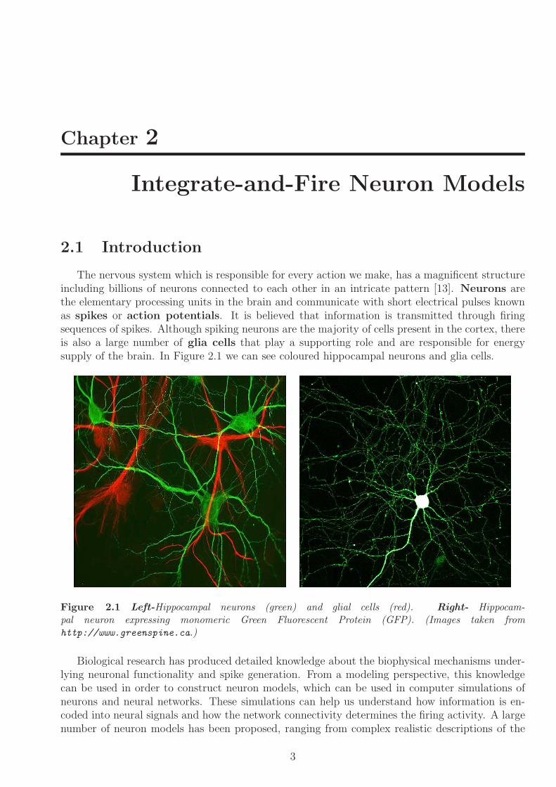
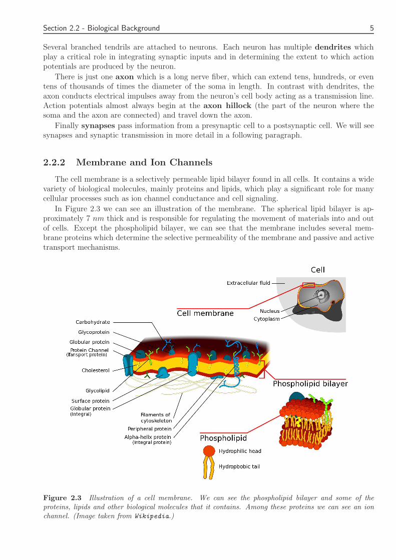
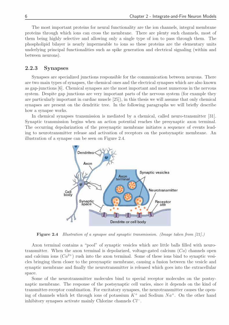
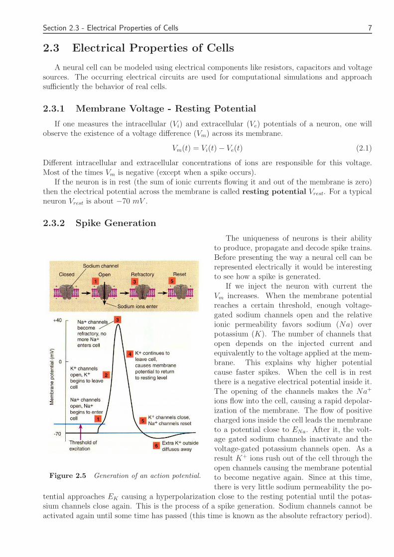
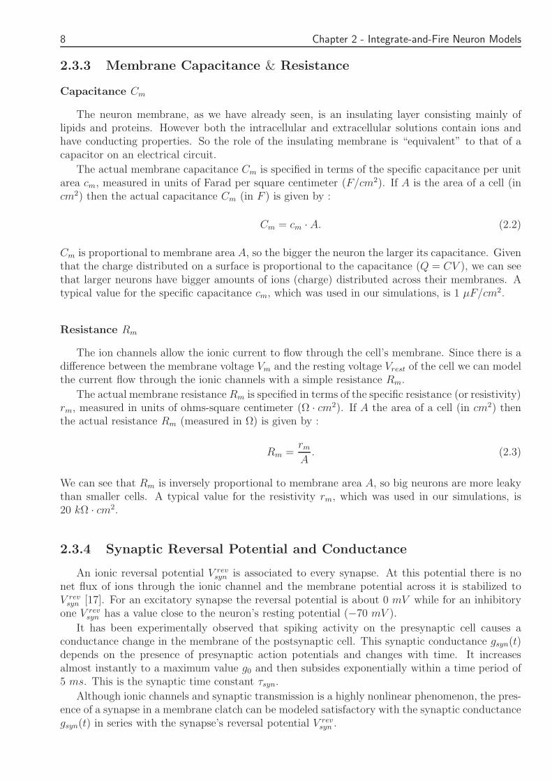
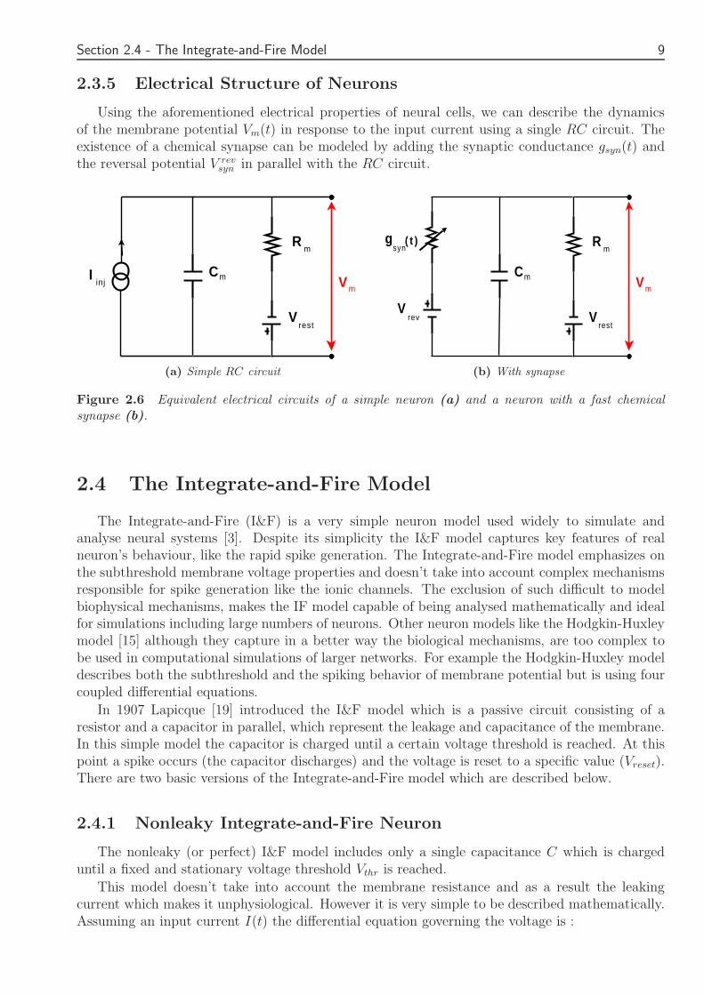
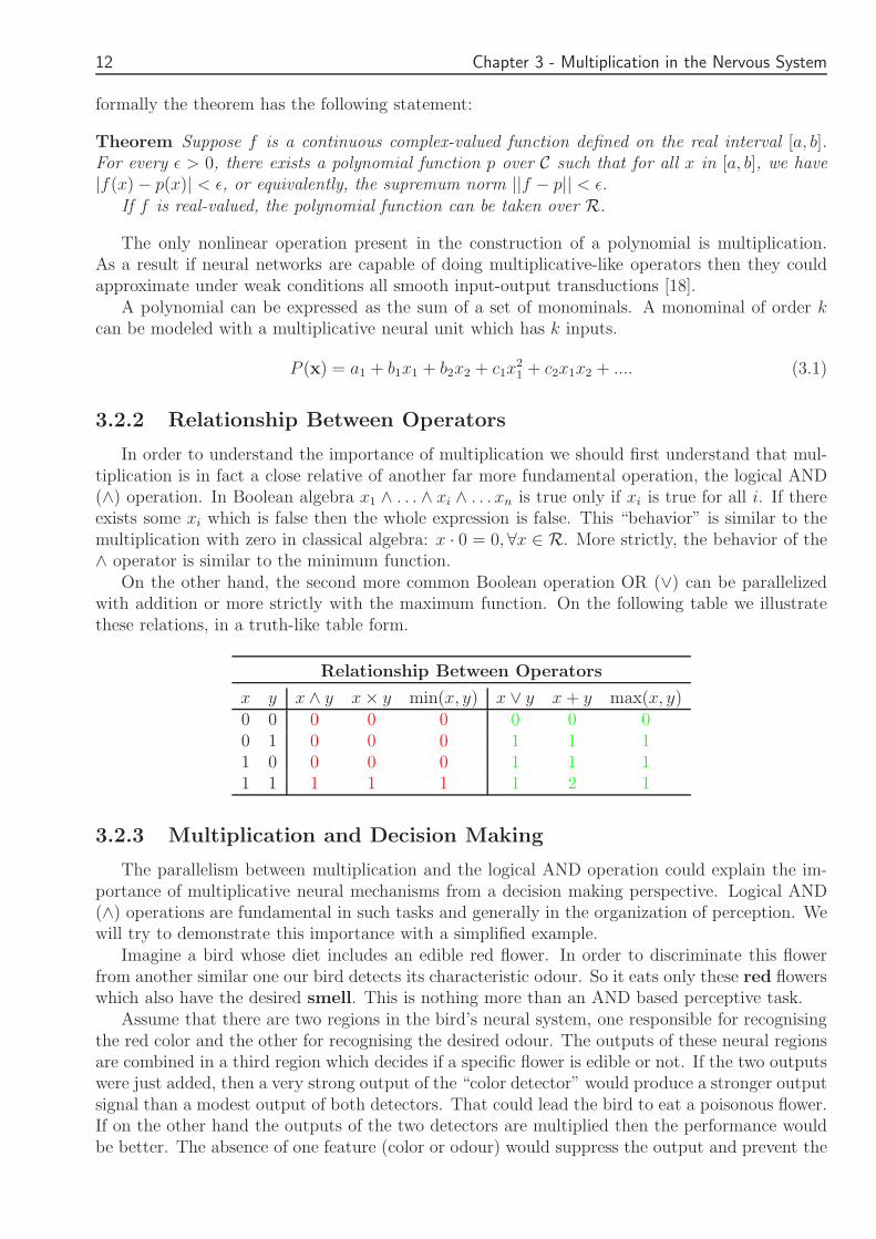
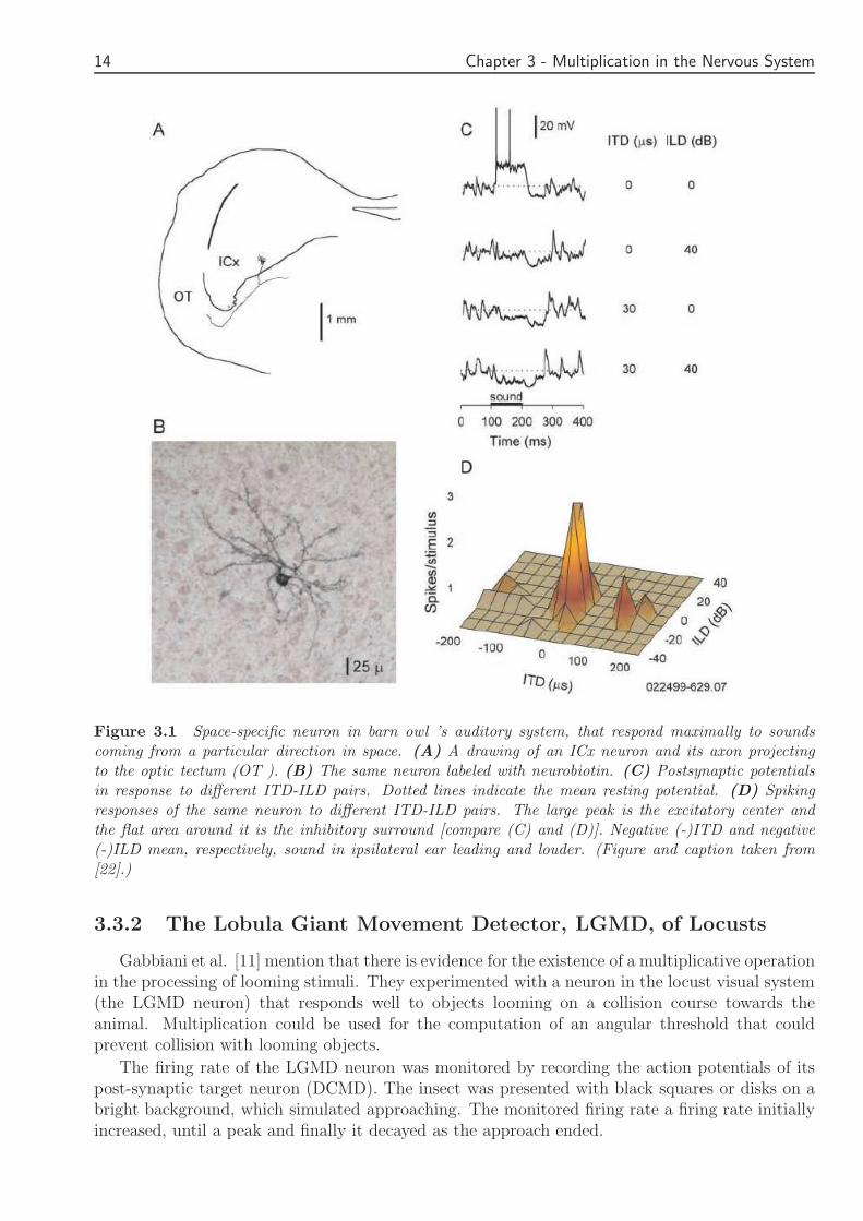
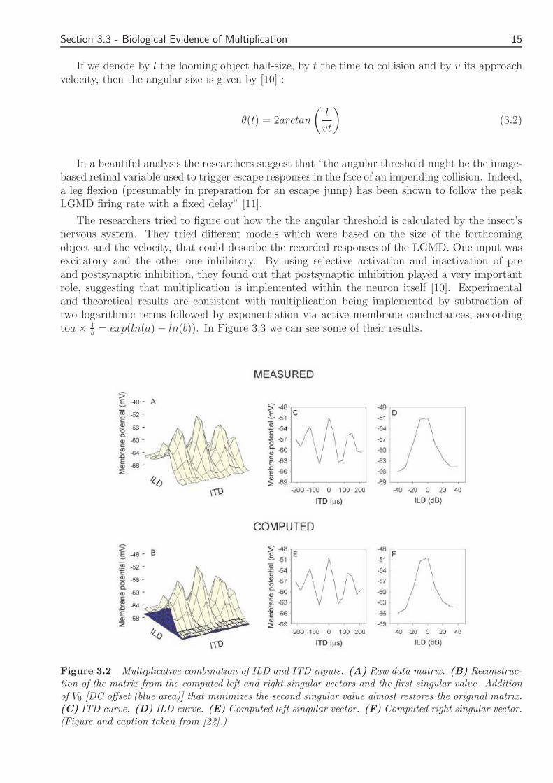
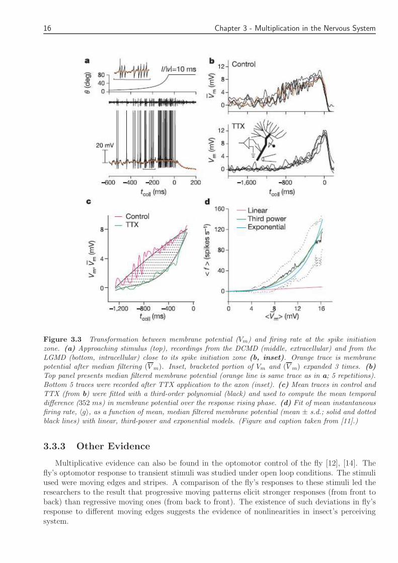
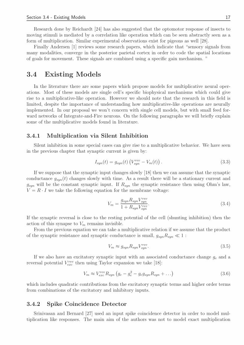
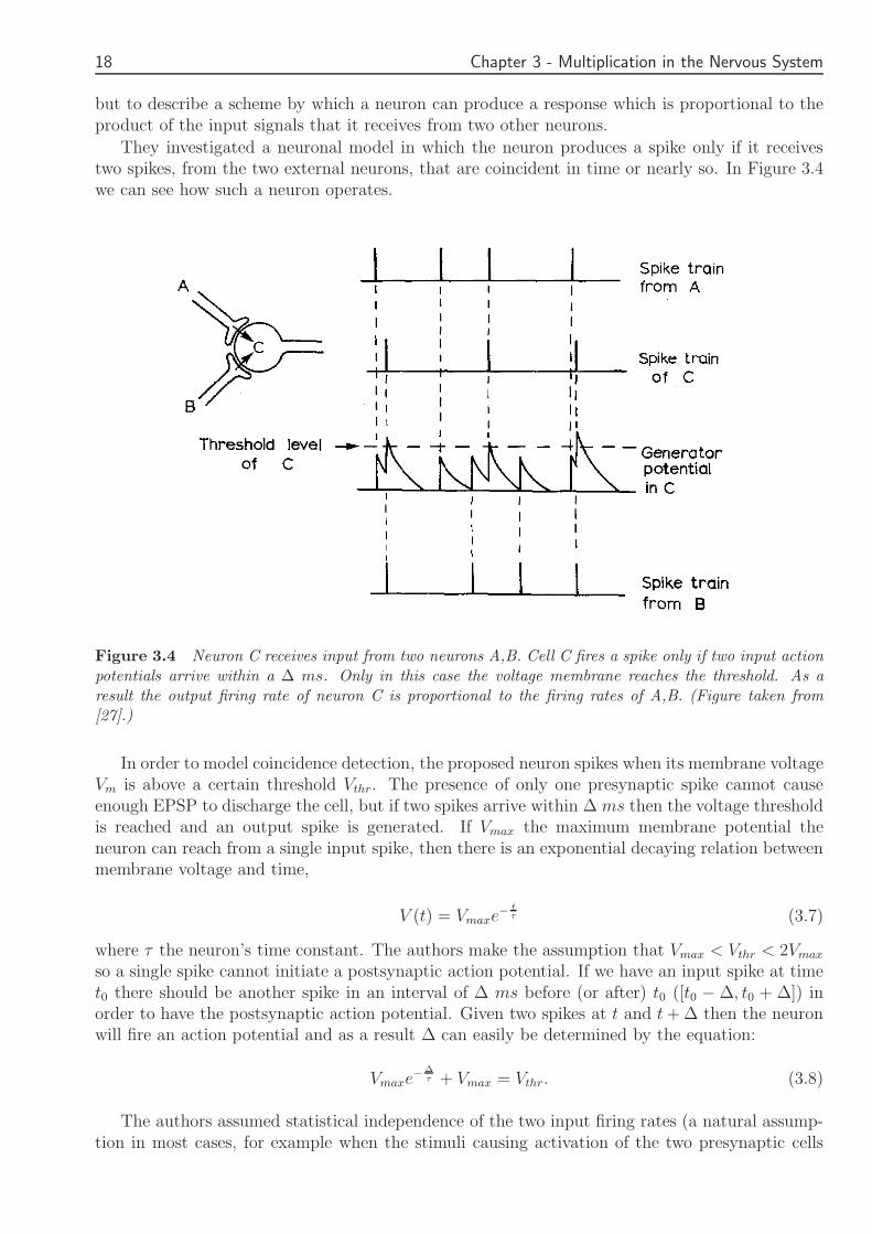
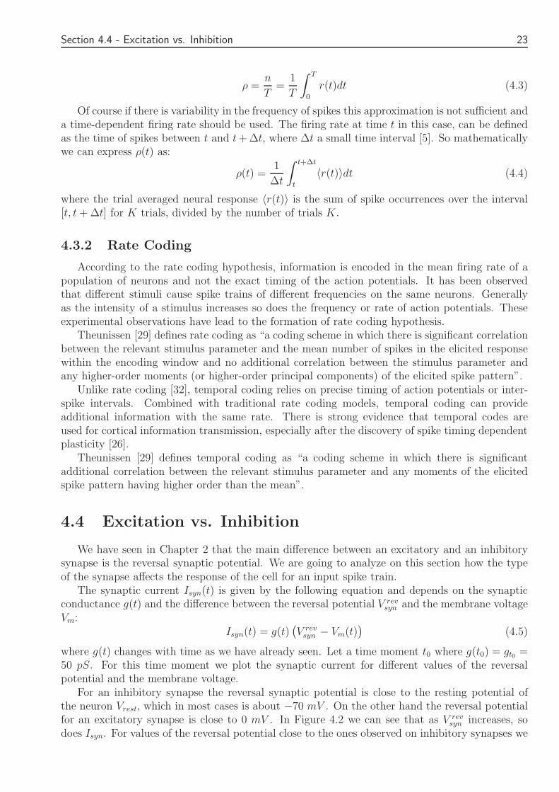
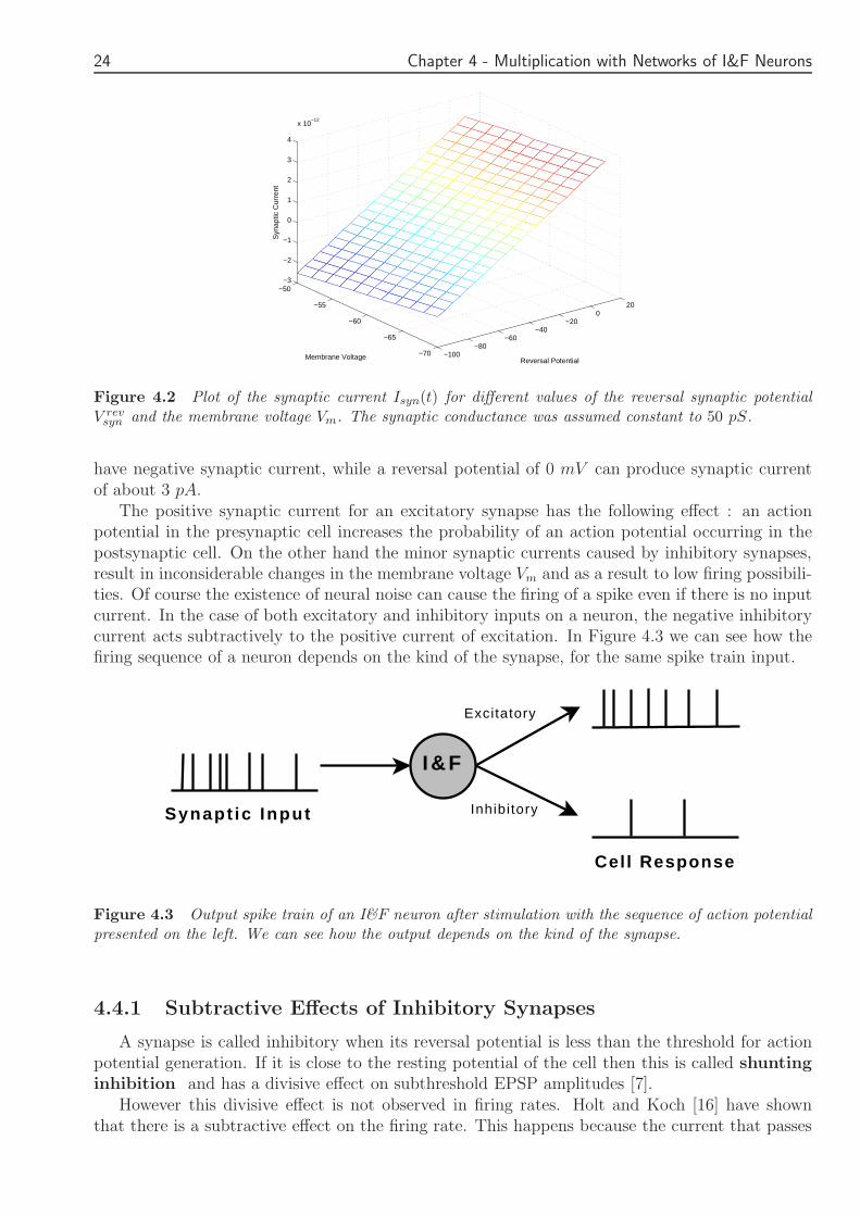
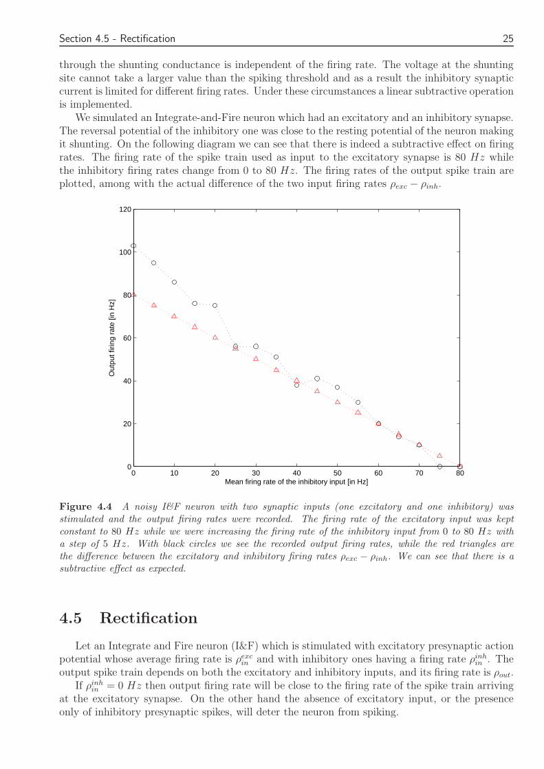
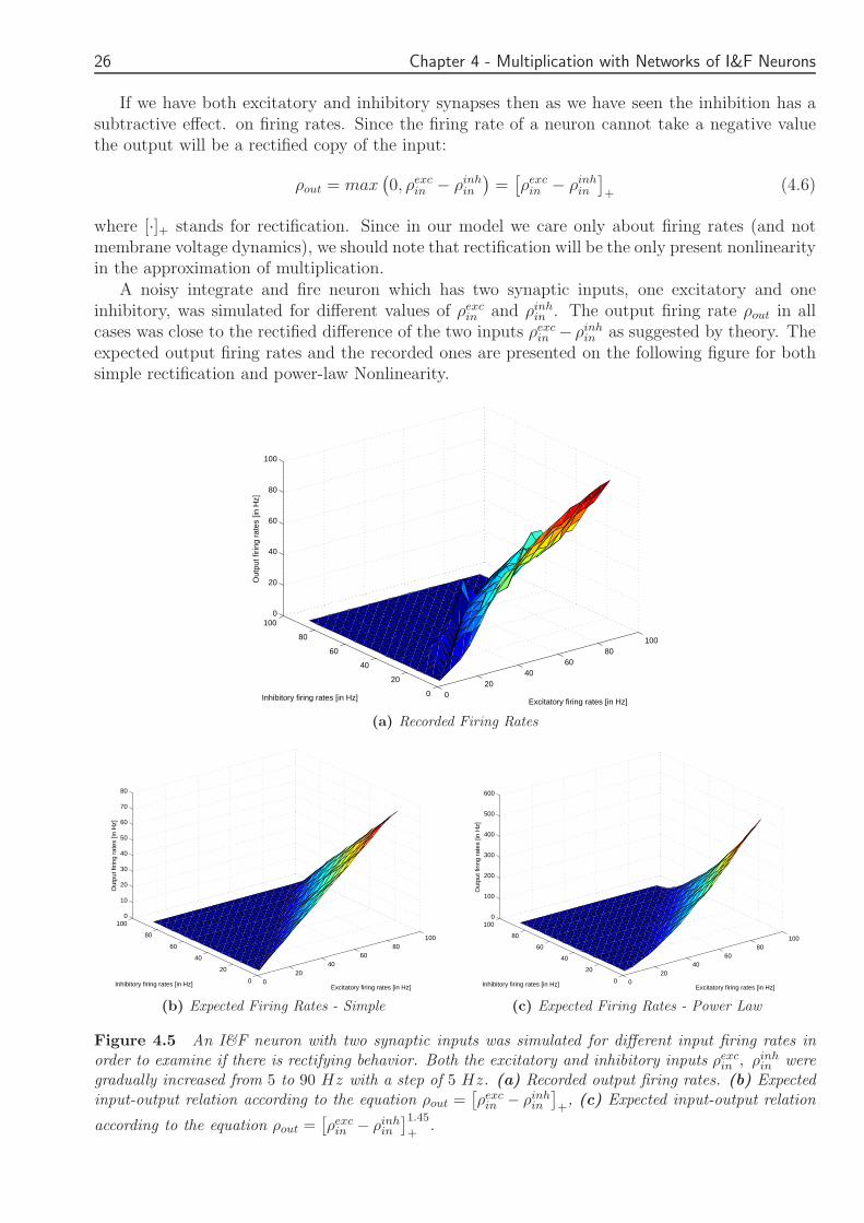
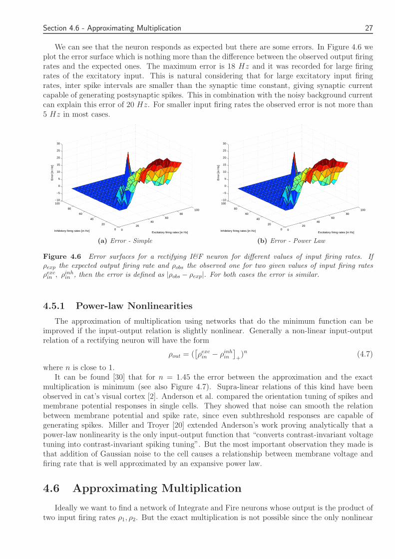
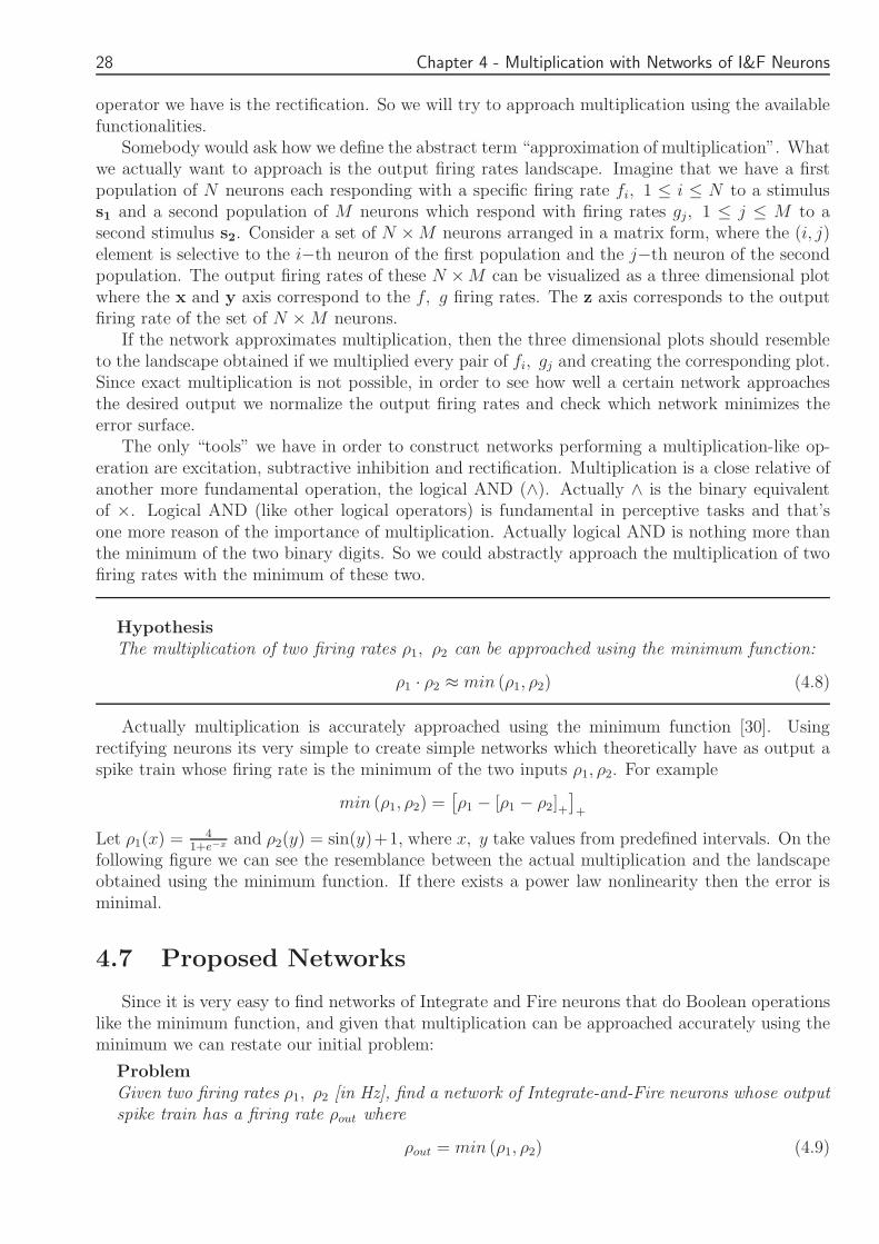
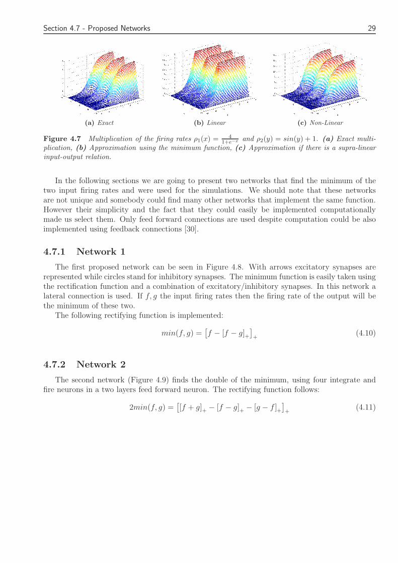
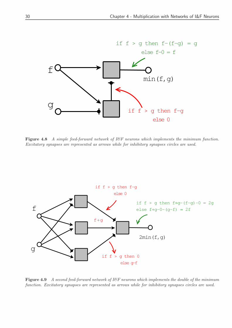
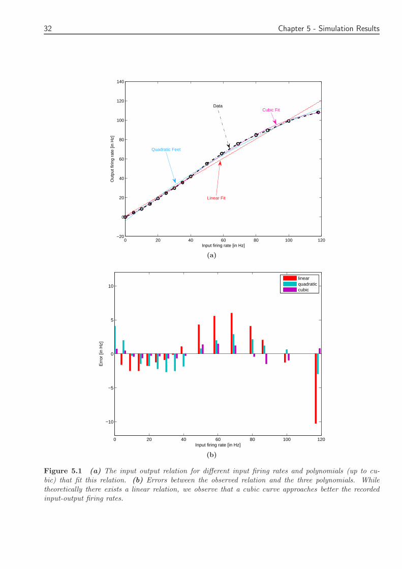
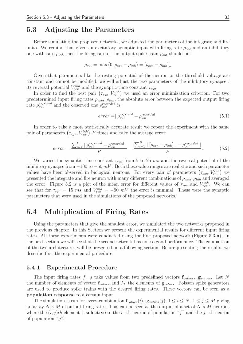
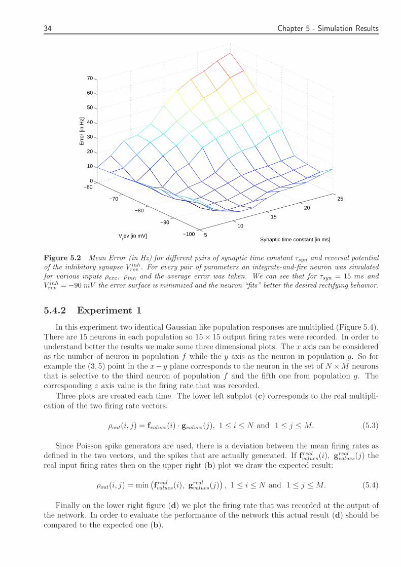
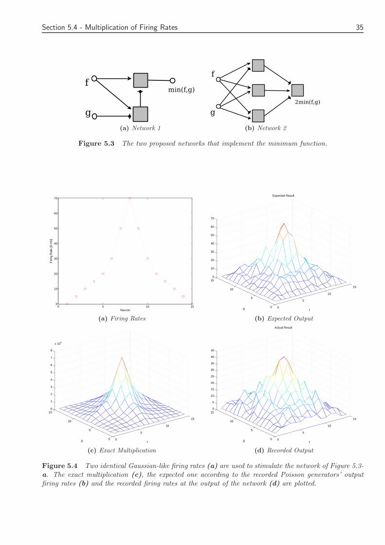
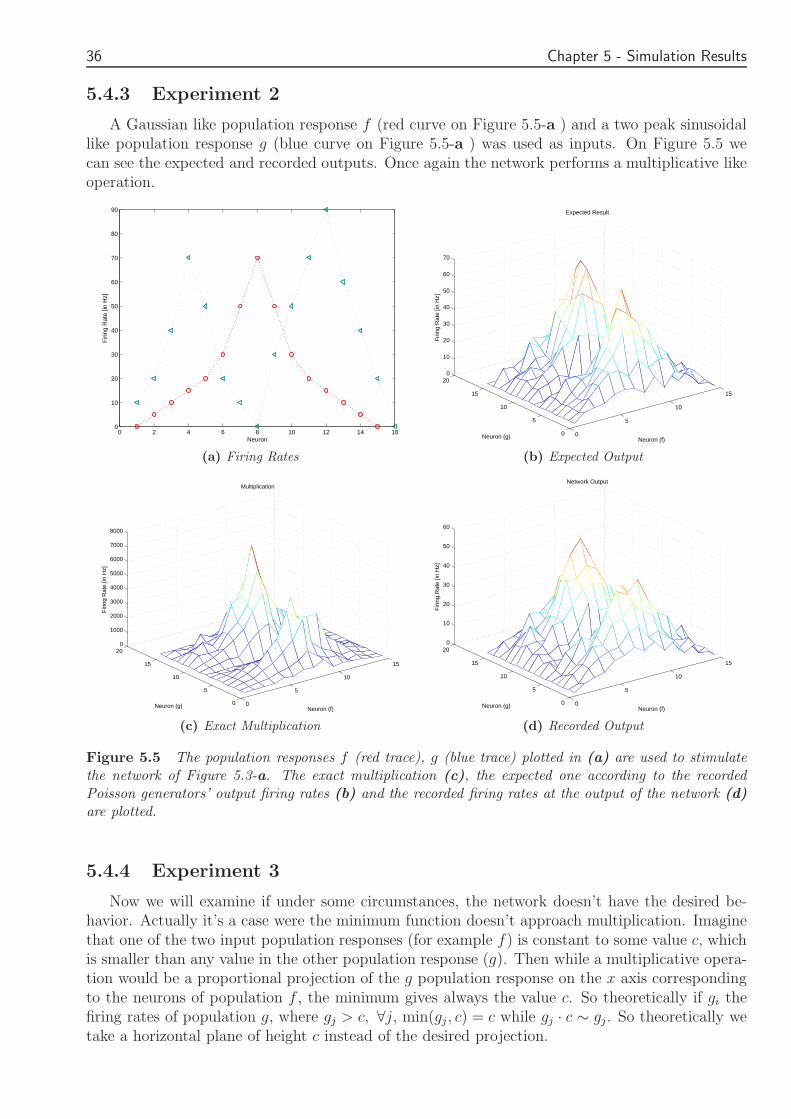
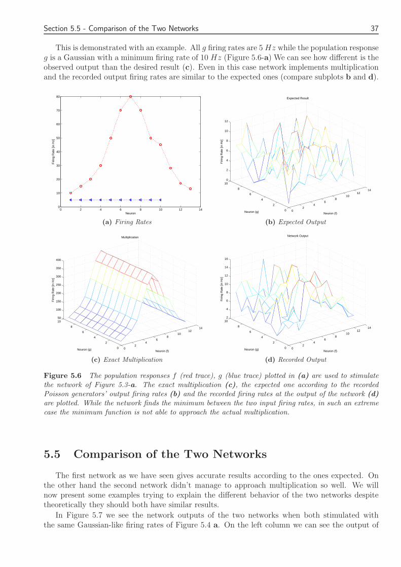
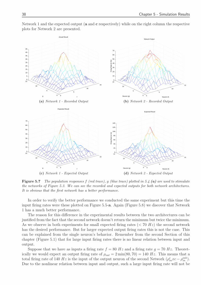
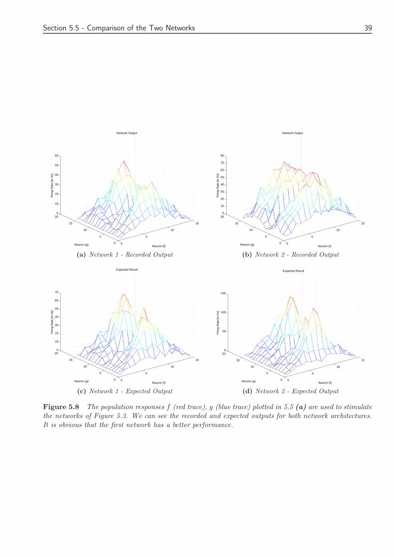
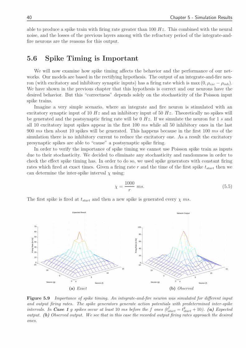
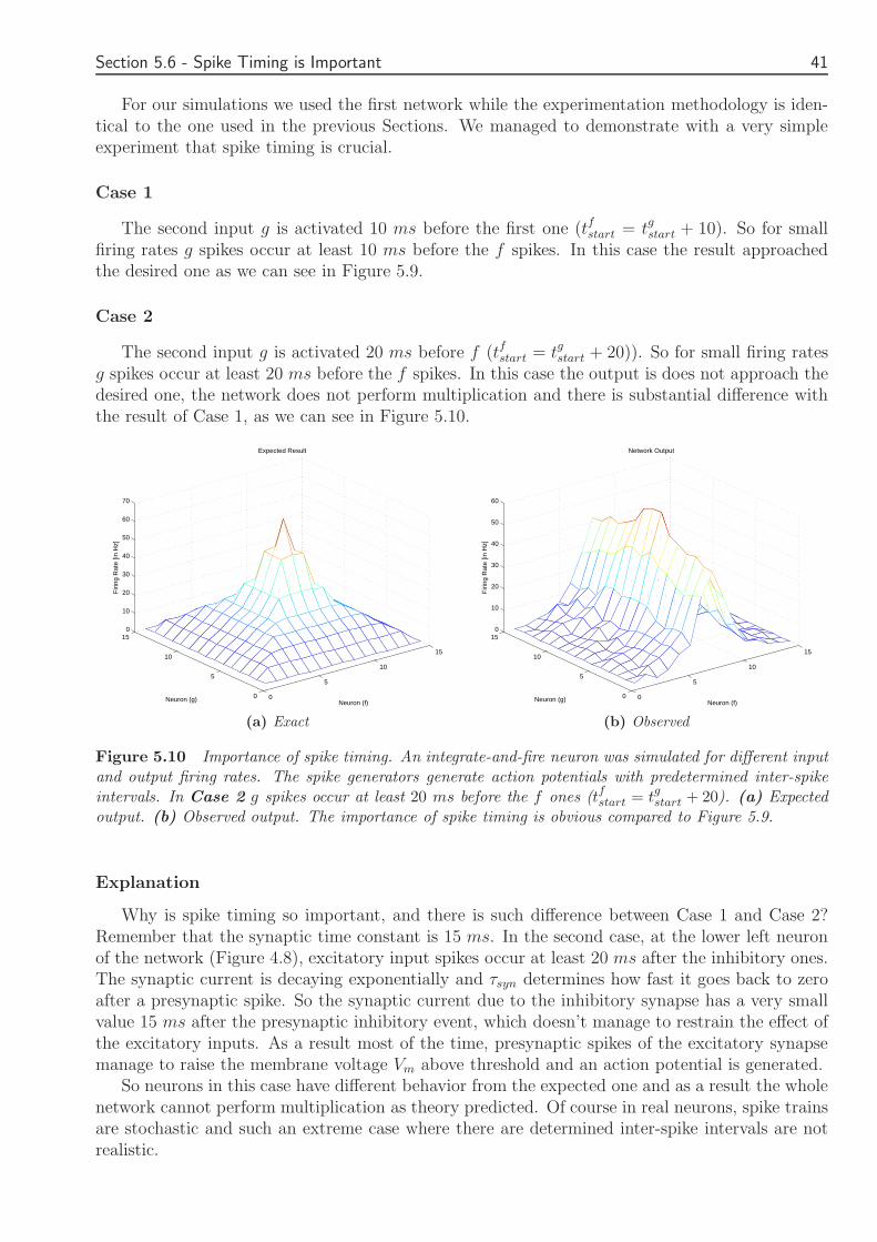
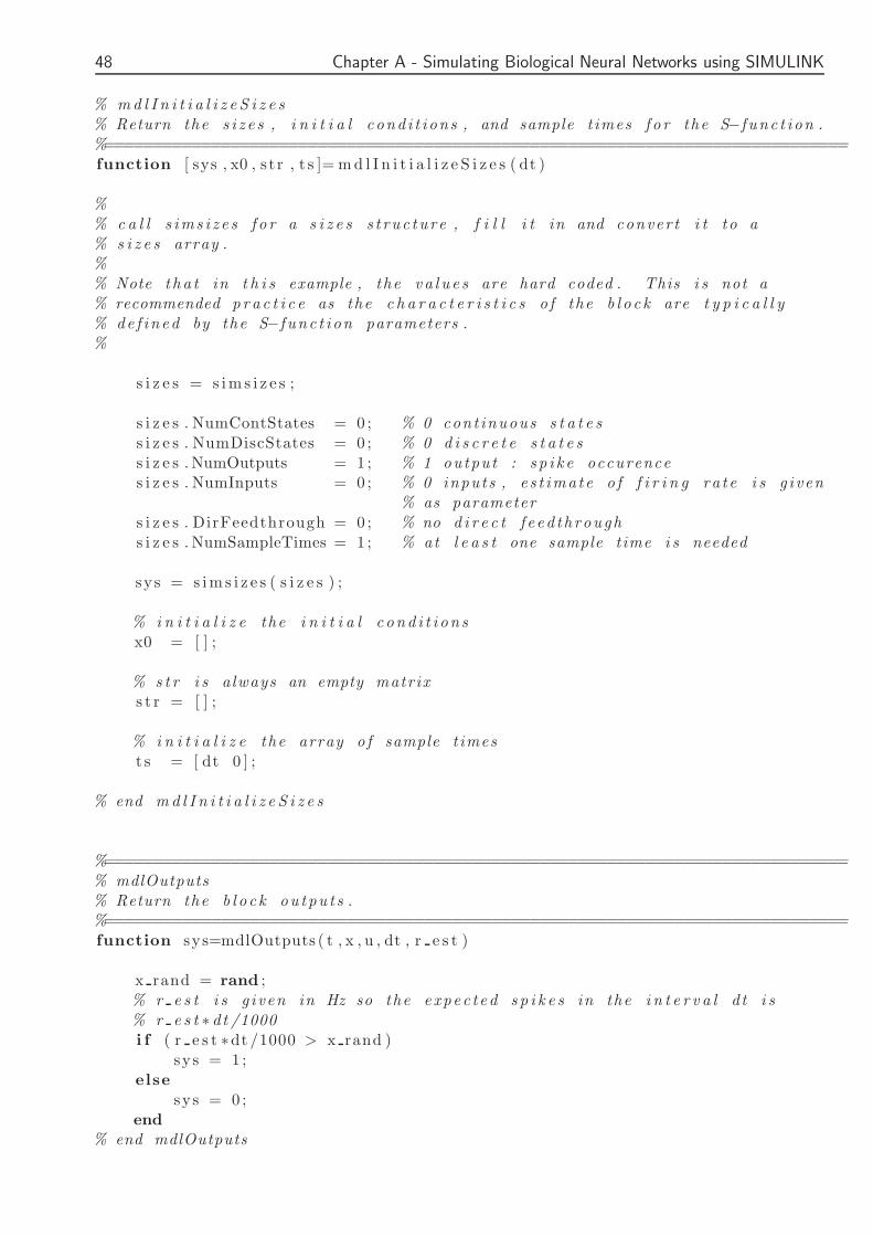
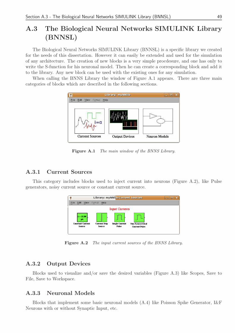
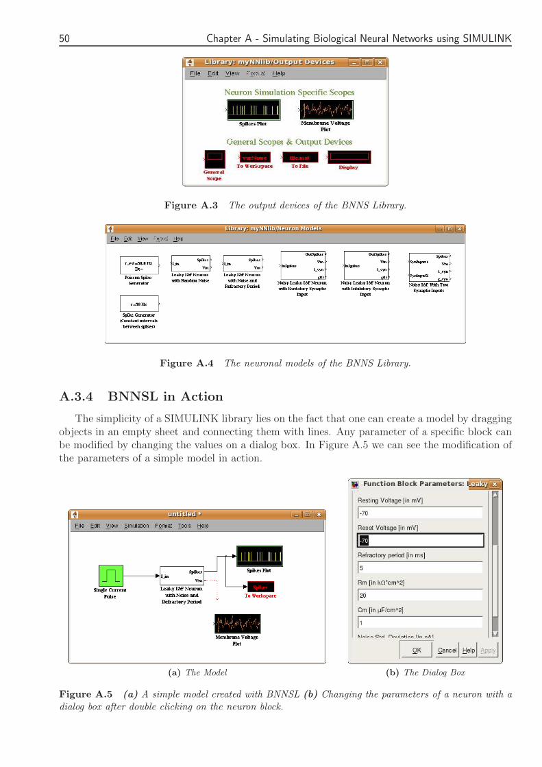
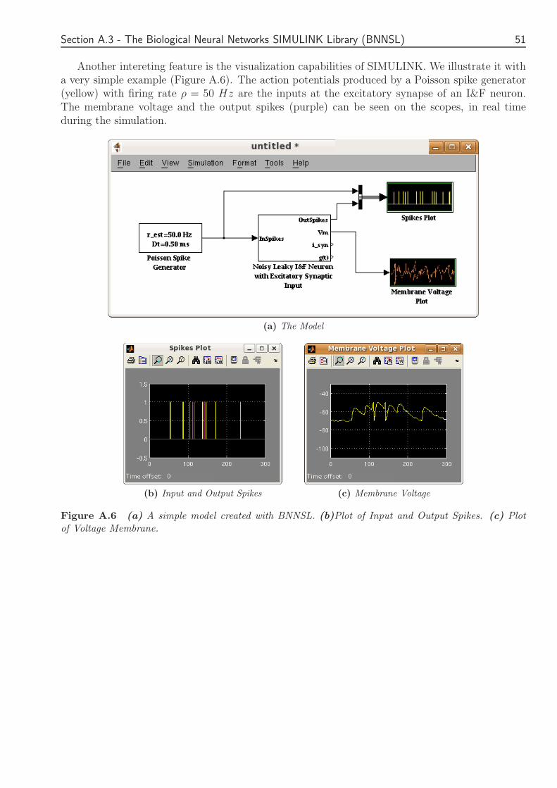