Embed Size (px)
DESCRIPTION
Muon simulations. Anna Kiseleva. Outline. Muon system 2006 New Mu on Ch amber system ( MuCh ) Track finding und selection Results for low-mass vector mesons J/ ψ simulations Detector resolution study: preliminary results Conclusions and next steps. MuCh system 2006. - PowerPoint PPT Presentation
Citation preview
Muon simulationsMuon simulations
Anna Kiseleva
OutlineOutline
• Muon system 2006
• New Muon Chamber system (MuCh)
• Track finding und selection
• Results for low-mass vector mesons
• J/ψ simulations
• Detector resolution study: preliminary results
• Conclusions and next steps
• Muon system 2006
• New Muon Chamber system (MuCh)
• Track finding und selection
• Results for low-mass vector mesons
• J/ψ simulations
• Detector resolution study: preliminary results
• Conclusions and next steps
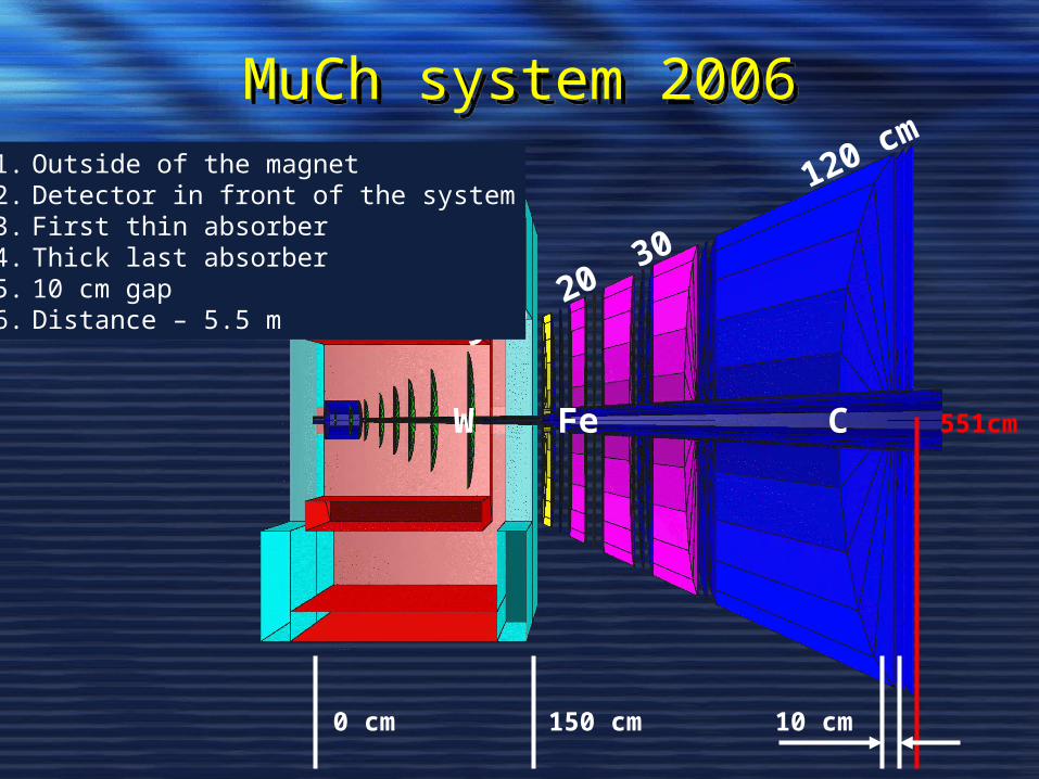
MuCh system 2006MuCh system 2006
5 10 20 30
120 cm
150 cm 10 cm
W Fe C
0 cm
551cm
1. Outside of the magnet2. Detector in front of the system3. First thin absorber4. Thick last absorber5. 10 cm gap 6. Distance – 5.5 m
ProblemsProblems
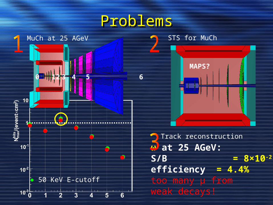
● 50 KeV E-cutoff
ω at 25 AGeV:S/B = 8×10⁻²
efficiency = 4.4%too many μ from weak decays!
MAPS?
MuCh at 25 AGeV STS for MuCh
Track reconstruction
0 12 3 4 5 6
ProblemsProblems
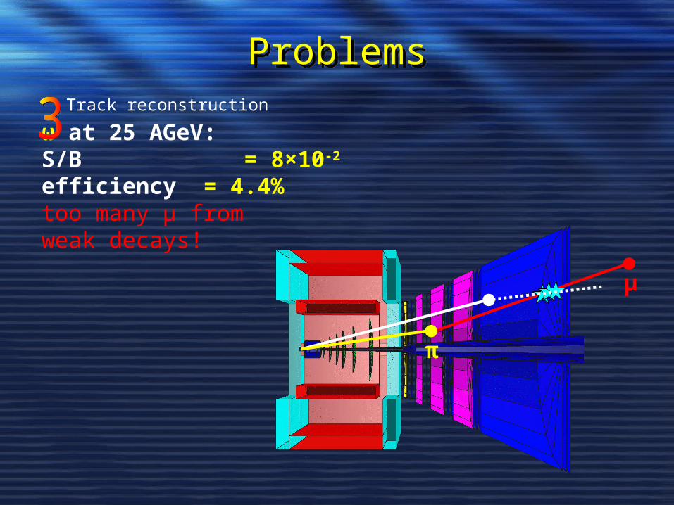
ω at 25 AGeV:S/B = 8×10⁻²
efficiency = 4.4%too many μ from weak decays!
Track reconstruction
π
μ
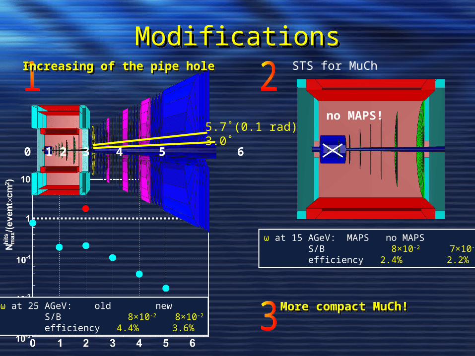
ModificationsModifications
no MAPS!
STS for MuCh
More compact MuCh!More compact MuCh!
0 1 2 3 4 5 6
ω at 25 AGeV: old new S/B 8×10⁻² 8×10⁻²
efficiency 4.4% 3.6%
5.7˚(0.1 rad)3.0˚
ω at 15 AGeV: MAPS no MAPS S/B 8×10⁻² 7×10⁻²
efficiency 2.4% 2.2%
Increasing of the pipe holeIncreasing of the pipe hole
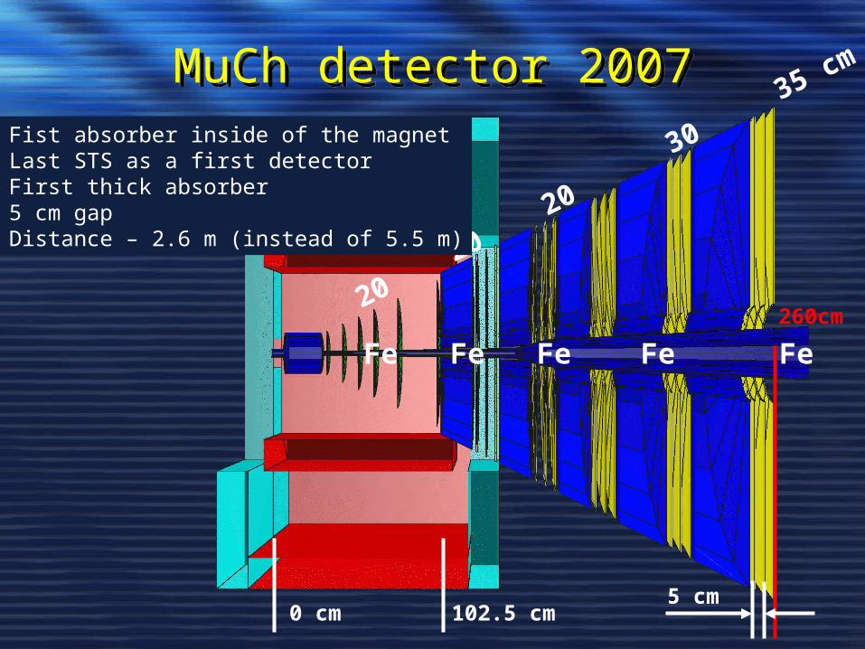
MuCh detector 2007MuCh detector 2007
Fe Fe Fe Fe Fe
20 20 2
0 30
35 cm
102.5 cm0 cm5 cm
260cm
1. Fist absorber inside of the magnet2. Last STS as a first detector3. First thick absorber4. 5 cm gap 5. Distance – 2.6 m (instead of 5.5 m)
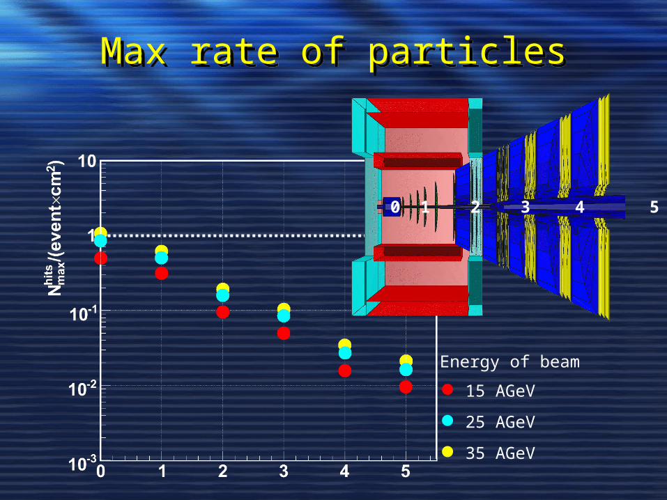
Max rate of particlesMax rate of particles
Energy of beam
● 15 AGeV
● 25 AGeV
● 35 AGeV
0 1 2 3 4 5
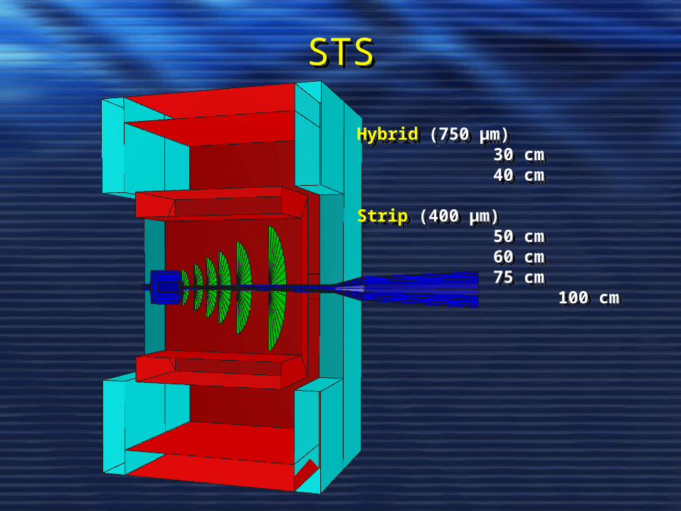
STSSTS
Hybrid (750 μm) 30 cm 40 cm
Strip (400 μm) 50 cm
60 cm75 cm
100 cm
Hybrid (750 μm) 30 cm 40 cm
Strip (400 μm) 50 cm
60 cm75 cm
100 cm
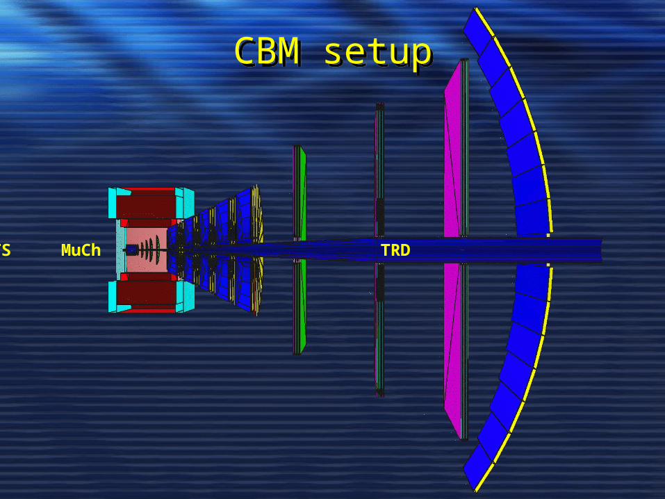
CBM setupCBM setup
STS MuCh TRD ToF
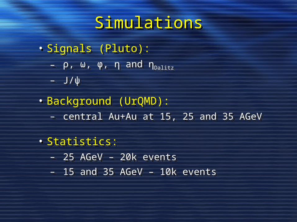
SimulationsSimulations
• Signals (Pluto):
– ρ, ω, φ, η and ηDalitz
– J/ψ
• Background (UrQMD):– central Au+Au at 15, 25 and 35 AGeV
• Statistics:– 25 AGeV – 20k events
– 15 and 35 AGeV – 10k events
• Signals (Pluto):
– ρ, ω, φ, η and ηDalitz
– J/ψ
• Background (UrQMD):– central Au+Au at 15, 25 and 35 AGeV
• Statistics:– 25 AGeV – 20k events
– 15 and 35 AGeV – 10k events
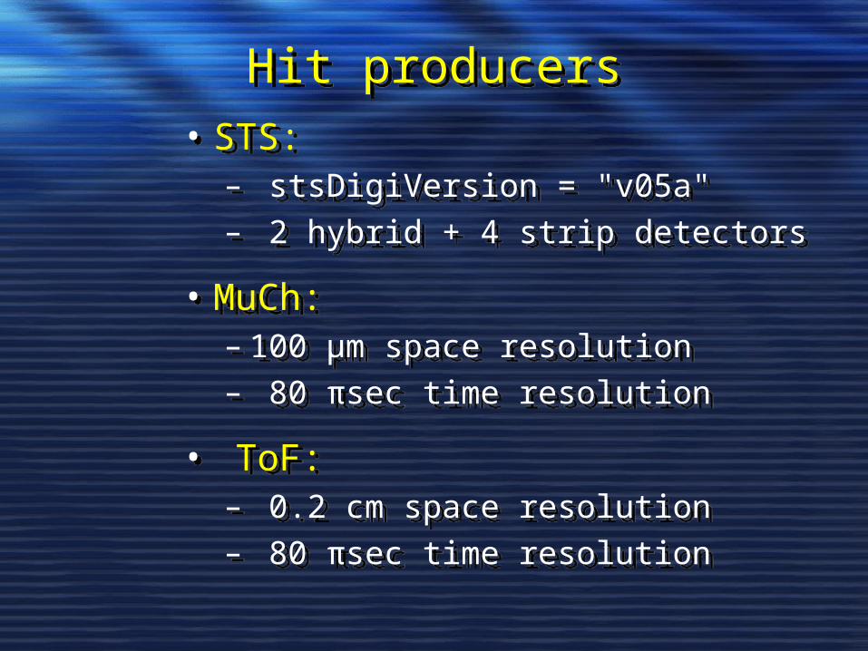
Hit producersHit producers
• STS:– stsDigiVersion = "v05a"– 2 hybrid + 4 strip detectors
• MuCh:– 100 μm space resolution– 80 πsec time resolution
• ToF:– 0.2 cm space resolution– 80 πsec time resolution
• STS:– stsDigiVersion = "v05a"– 2 hybrid + 4 strip detectors
• MuCh:– 100 μm space resolution– 80 πsec time resolution
• ToF:– 0.2 cm space resolution– 80 πsec time resolution
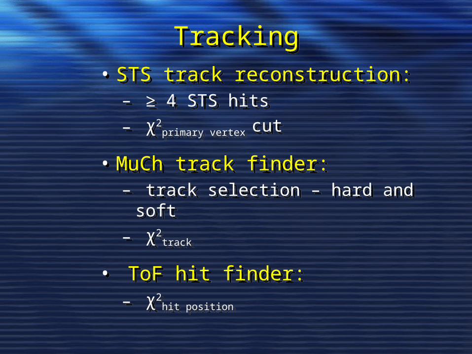
TrackingTracking
• STS track reconstruction:– ≥ 4 STS hits
– χ2primary vertex cut
• MuCh track finder:– track selection – hard and soft
– χ2track
• ToF hit finder:– χ2
hit position
• STS track reconstruction:– ≥ 4 STS hits
– χ2primary vertex cut
• MuCh track finder:– track selection – hard and soft
– χ2track
• ToF hit finder:– χ2
hit position
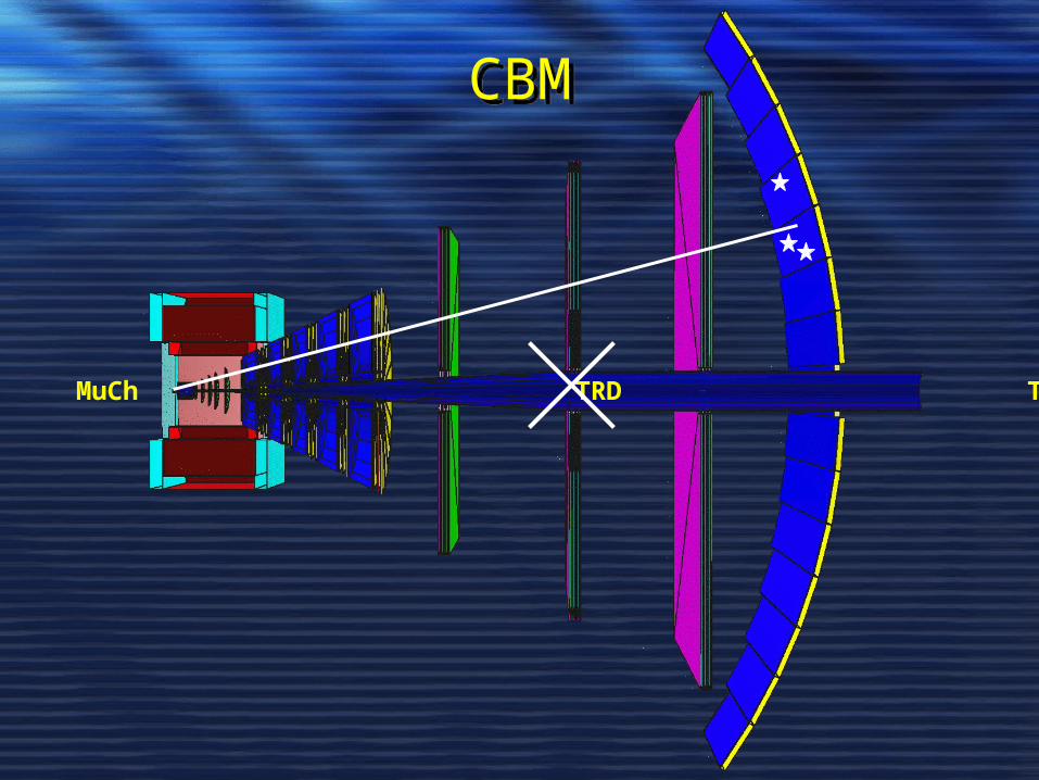
CBMCBM
STS MuCh TRD ToF
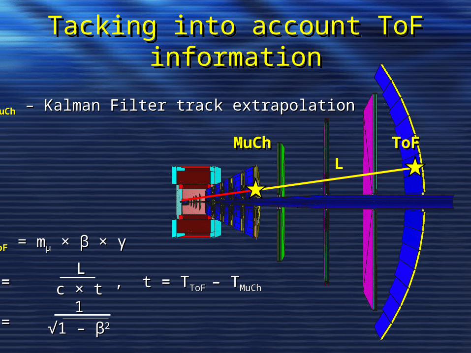
Tacking into account ToF information
Tacking into account ToF information
PPToFToF = m = mμμ × × ββ × × γγ
ββ = , t = T = , t = TToF ToF – T– TMuChMuCh
γγ = =
LLc × tc × t
√√1 – 1 – ββ22
11
PPMuChMuCh – Kalman Filter track extrapolation – Kalman Filter track extrapolation
MuChMuChL
ToFToF
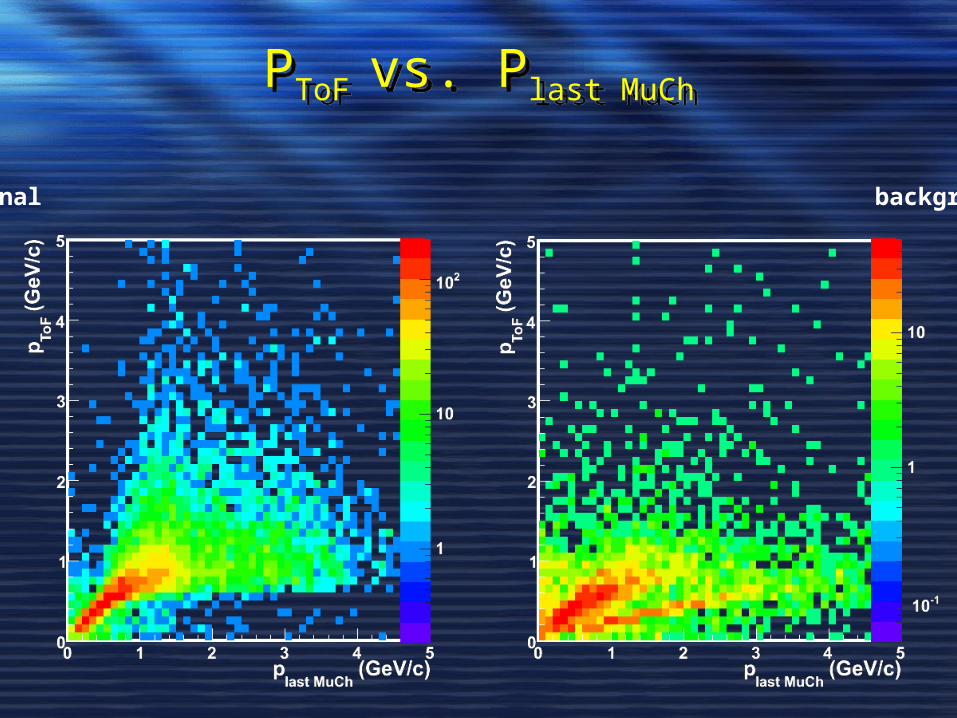
PToF vs. Plast MuChPToF vs. Plast MuCh
φ signal background
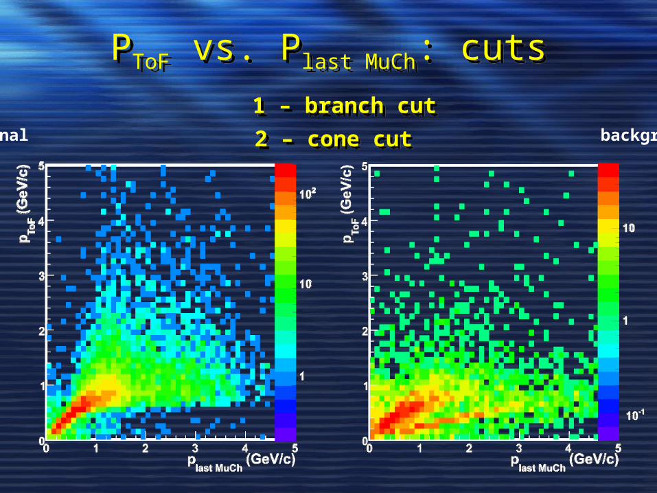
PToF vs. Plast MuCh: cutsPToF vs. Plast MuCh: cuts
φ signal background
1 – branch cut1 – branch cut
2 – cone cut2 – cone cut
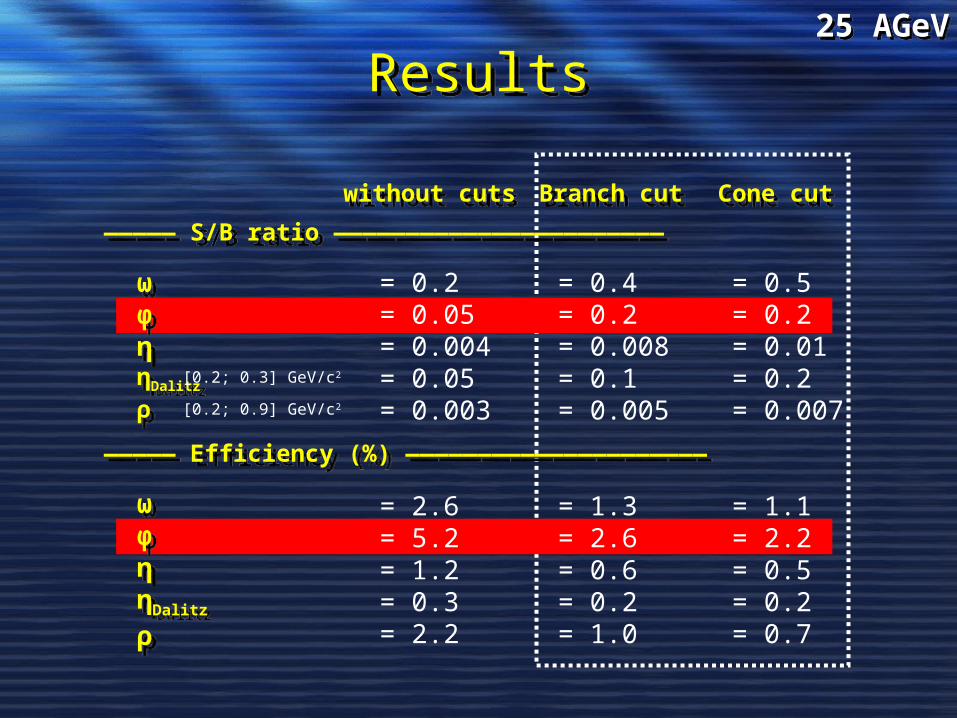
ResultsResults
= 0.5= 0.2= 0.01= 0.2= 0.007
= 1.1= 2.2= 0.5= 0.2= 0.7
= 0.4= 0.2= 0.008= 0.1= 0.005
= 1.3= 2.6= 0.6= 0.2= 1.0
= 0.2= 0.05= 0.004= 0.05= 0.003
= 2.6= 5.2= 1.2= 0.3= 2.2
————— S/B ratio ———————————————————————————— S/B ratio ———————————————————————
Branch cutBranch cut Cone cutCone cut
————— Efficiency (%) —————————————————————————— Efficiency (%) —————————————————————
ωφηηDalitz
ρ
ωφηηDalitz
ρ
ωφηηDalitz
ρ
ωφηηDalitz
ρ
[0.2; 0.9] GeV/c2
[0.2; 0.3] GeV/c2
without cutswithout cuts
25 AGeV25 AGeV
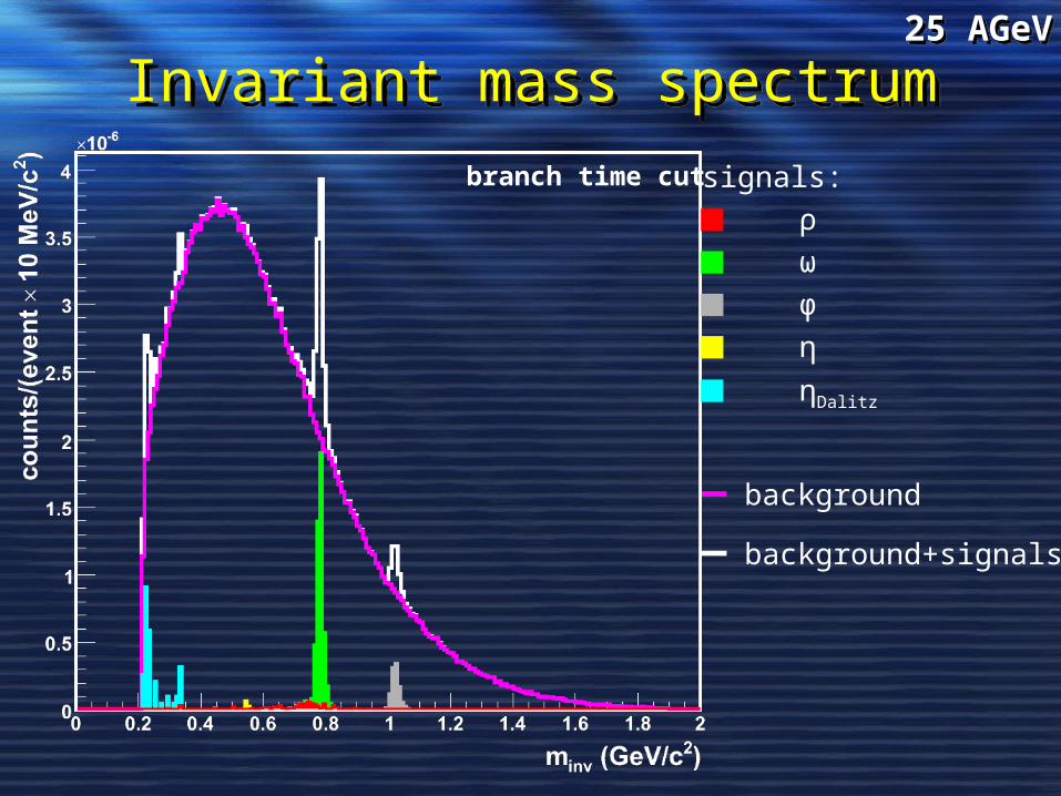
Invariant mass spectrumInvariant mass spectrum
signals:
ρ
ω
φ
η
ηDalitz
— background
— background+signals
branch time cut
25 AGeV25 AGeV
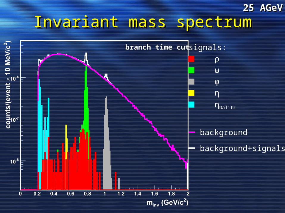
Invariant mass spectrumInvariant mass spectrum
signals:
ρ
ω
φ
η
ηDalitz
— background
— background+signals
branch time cut
25 AGeV25 AGeV
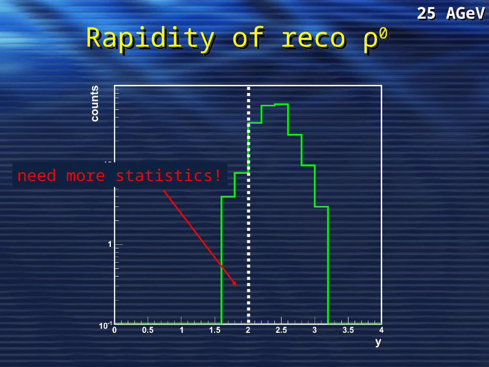
Rapidity of reco ρ0 Rapidity of reco ρ0
need more statistics!
25 AGeV25 AGeV
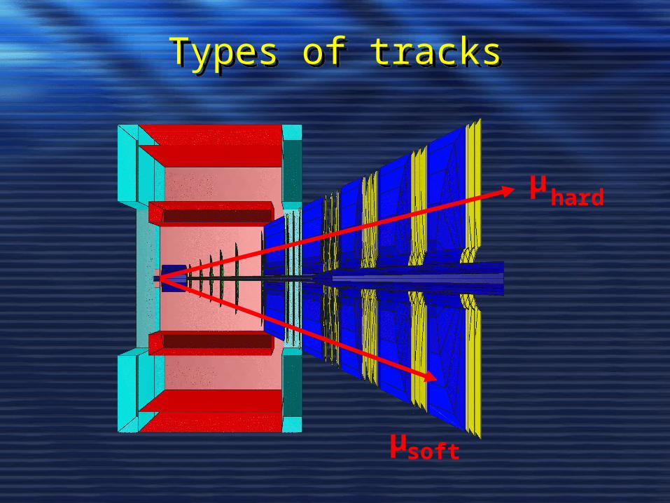
Types of tracksTypes of tracks
soft
μ
μ
hard
mean ± 2σmean ± 2σ
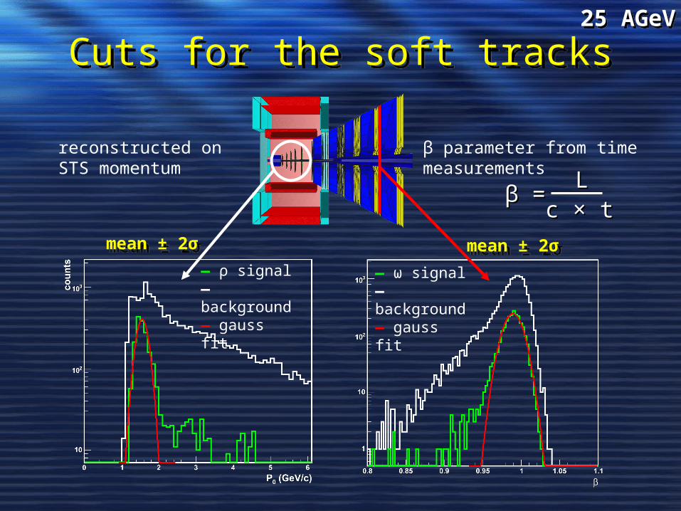
— ρ signal— background— gauss fit
Cuts for the soft tracksCuts for the soft tracks
— ω signal— background— gauss fit
mean ± 2σmean ± 2σ
reconstructed on STS momentum
β parameter from timemeasurements
ββ = =LL
c × tc × t
25 AGeV25 AGeV
ωφηηDalitz
ρ
ωφηηDalitz
ρ
ωφηηDalitz
ρ
ωφηηDalitz
ρ
[0.2; 0.9] GeV/c2
[0.2; 0.3] GeV/c2
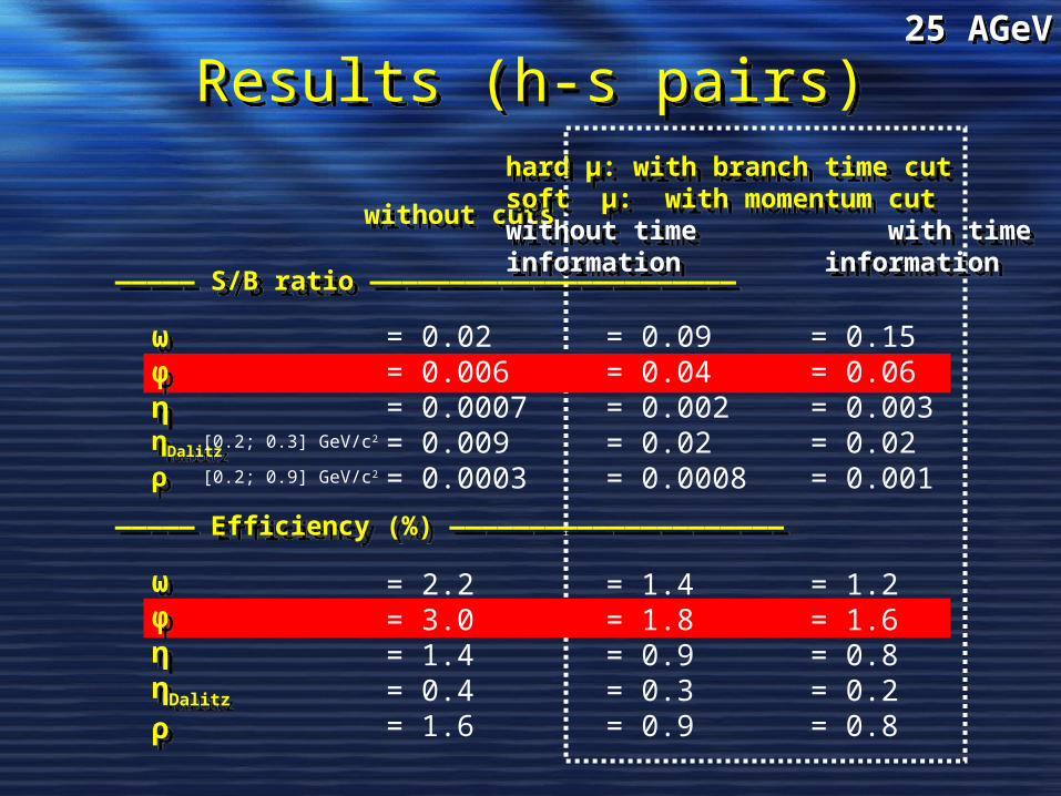
Results (h-s pairs)Results (h-s pairs)
= 0.15= 0.06= 0.003= 0.02= 0.001
= 1.2= 1.6= 0.8= 0.2= 0.8
= 0.02= 0.006= 0.0007= 0.009= 0.0003
= 2.2= 3.0= 1.4= 0.4= 1.6
————— S/B ratio ———————————————————————————— S/B ratio ———————————————————————
————— Efficiency (%) —————————————————————————— Efficiency (%) —————————————————————
without cutswithout cuts
hard μ: with branch time cutsoft μ: with momentum cutwithout time with timeinformation information
hard μ: with branch time cutsoft μ: with momentum cutwithout time with timeinformation information
= 0.09= 0.04= 0.002= 0.02= 0.0008
= 1.4= 1.8= 0.9= 0.3= 0.9
25 AGeV25 AGeV
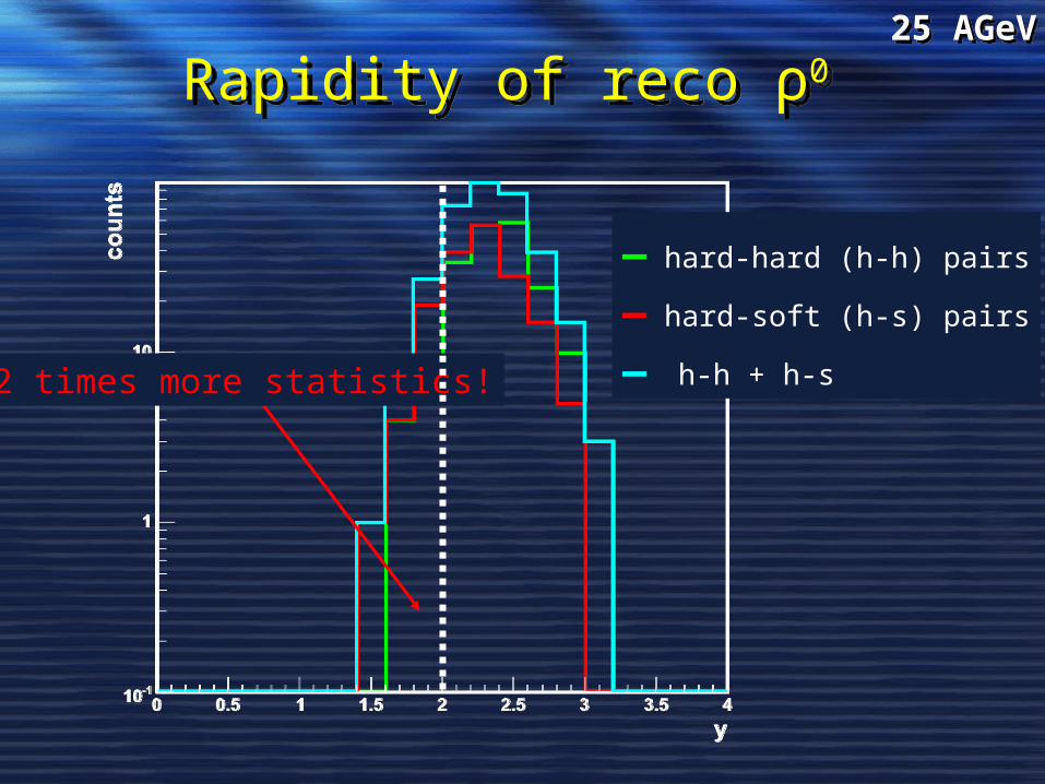
Rapidity of reco ρ0 Rapidity of reco ρ0
— hard-hard (h-h) pairs
— hard-soft (h-s) pairs
— h-h + h-s2 times more statistics!
25 AGeV25 AGeV
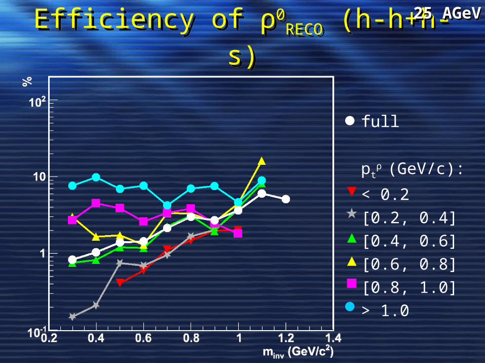
Efficiency of ρ0RECO (h-h+h-s)Efficiency of ρ0RECO (h-h+h-s)
full
ptρ (GeV/c):
< 0.2
[0.2, 0.4]
[0.4, 0.6]
[0.6, 0.8]
[0.8, 1.0]
> 1.0
▼
▲
▲
25 AGeV25 AGeV
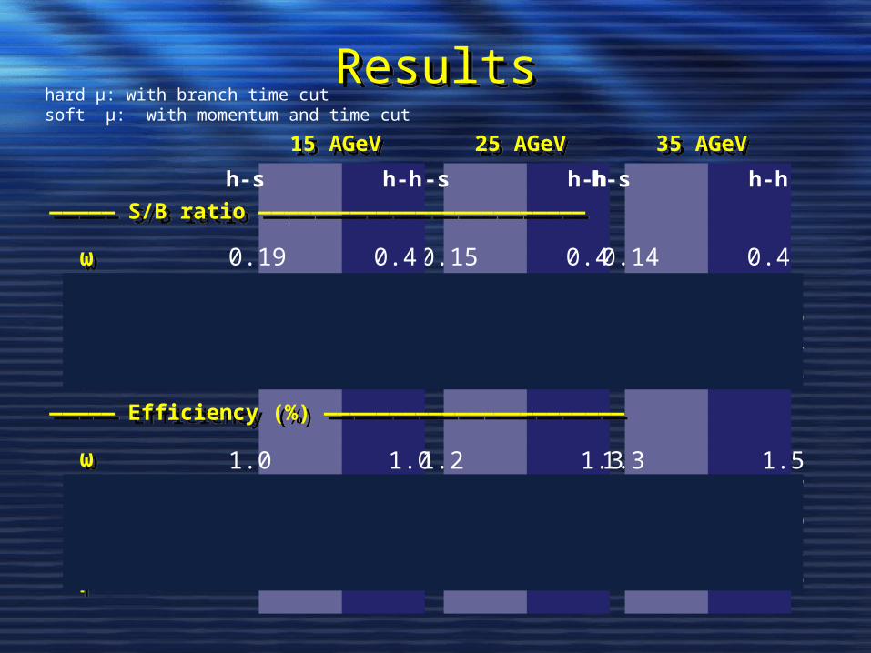
ResultsResults
0.15 0.40.06 0.20.003 0.0080.02 0.10.001 0.005
1.2 1.31.6 2.60.8 0.60.2 0.20.8 1.0
25 AGeV25 AGeV
h-s h-h
0.19 0.40.03 0.070.004 0.0080.04 0.050.002 0.003
1.0 1.01.0 1.40.7 0.40.3 0.060.8 0.4
15 AGeV15 AGeV
h-s h-h
0.14 0.40.05 0.10.002 0.0060.03 0.040.001 0.003
1.3 1.51.7 2.70.7 0.60.4 0.10.9 0.8
35 AGeV35 AGeV
h-s h-h
ωφηηDalitz
ρ
ωφηηDalitz
ρ
ωφηηDalitz
ρ
ωφηηDalitz
ρ
[0.2; 0.9] GeV/c2
[0.2; 0.3] GeV/c2
————— S/B ratio —————————————————————————————— S/B ratio —————————————————————————
————— Efficiency (%) ———————————————————————————— Efficiency (%) ———————————————————————
hard μ: with branch time cut soft μ: with momentum and time cut
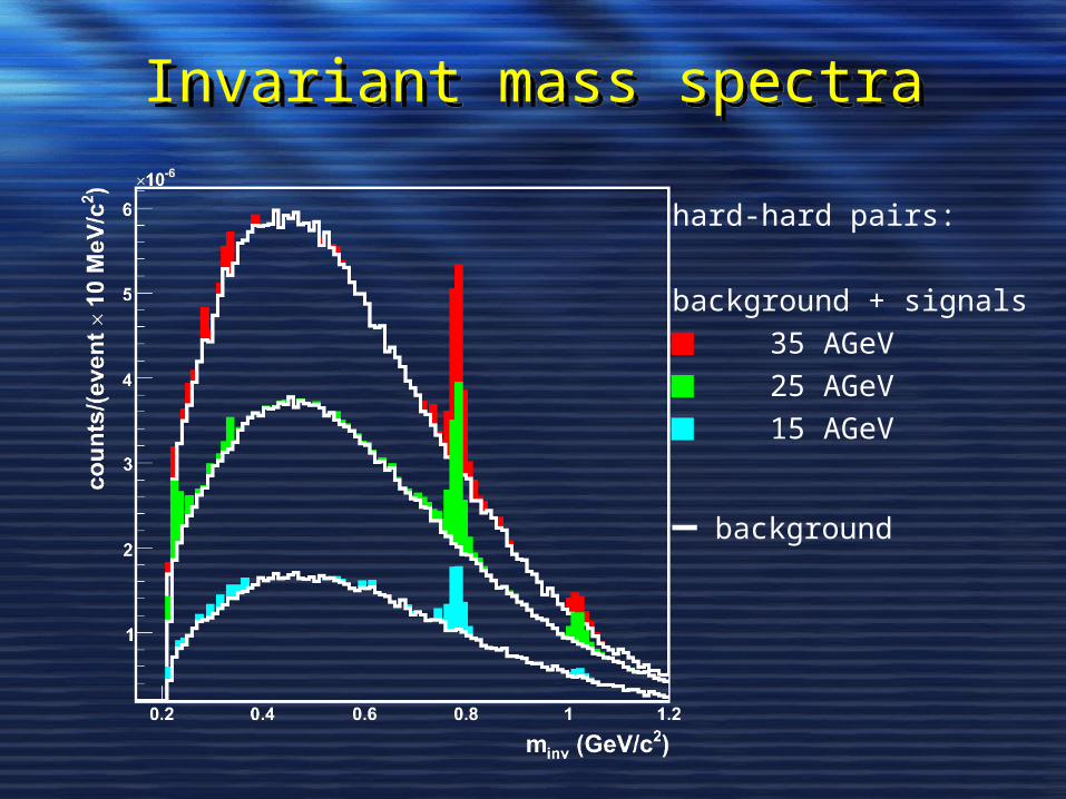
Invariant mass spectraInvariant mass spectra
hard-hard pairs:
background + signals
35 AGeV
25 AGeV
15 AGeV
— background
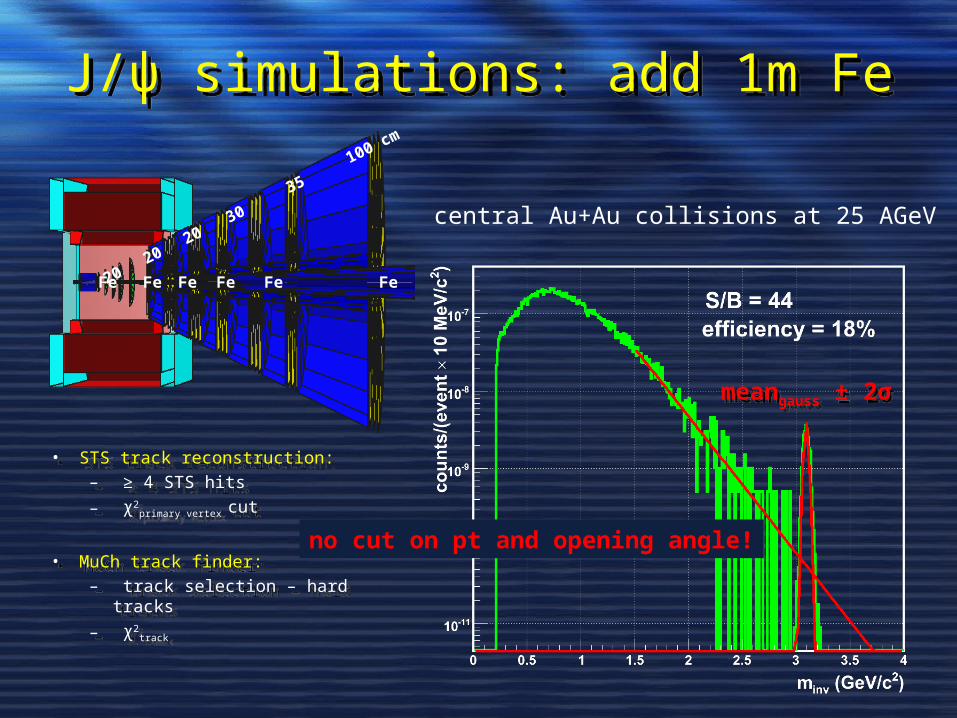
J/ψ simulations: add 1m FeJ/ψ simulations: add 1m Fe
Fe Fe Fe Fe Fe Fe
20 20 2
0 30
35 100 cm
central Au+Au collisions at 25 AGeV
• STS track reconstruction:– ≥ 4 STS hits
– χ2primary vertex cut
• MuCh track finder:– track selection – hard tracks
– χ2track
• STS track reconstruction:– ≥ 4 STS hits
– χ2primary vertex cut
• MuCh track finder:– track selection – hard tracks
– χ2track
no cut on pt and opening angle!
meangauss ± 2σmeangauss ± 2σ
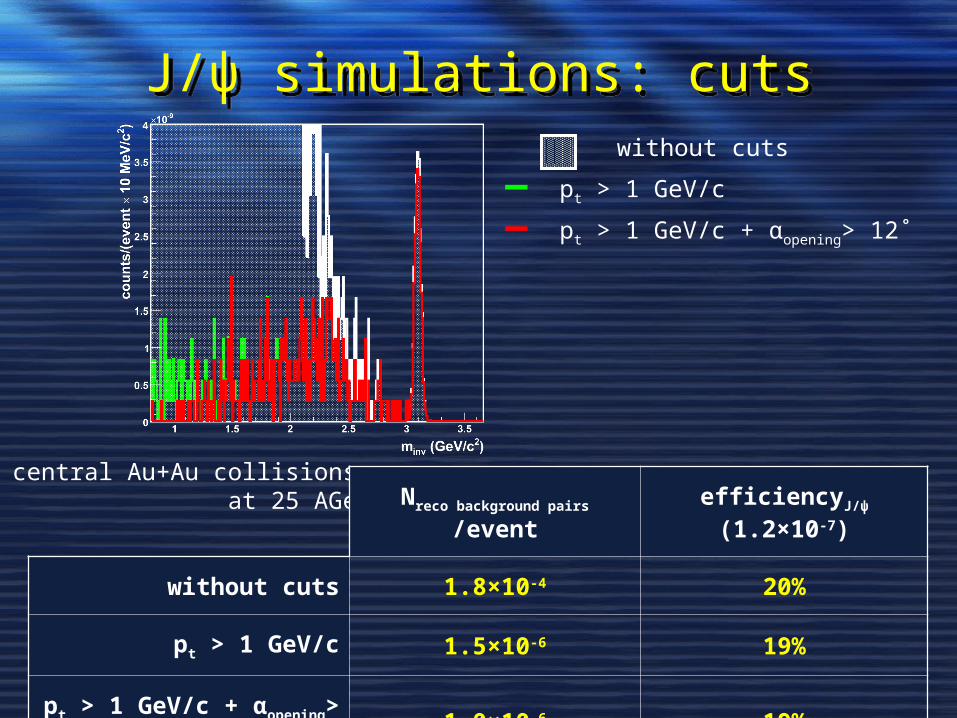
J/ψ simulations: cutsJ/ψ simulations: cuts
central Au+Au collisions at 25 AGeV
without cuts
— pt > 1 GeV/c
— pt > 1 GeV/c + αopening> 12˚
Nreco background pairs /event efficiencyJ/ψ (1.2×10⁻⁷)
without cuts 1.8×10⁻⁴ 20%
pt > 1 GeV/c 1.5×10⁻⁶ 19%
pt > 1 GeV/c + αopening> 12˚ 1.0×10⁻⁶ 19%
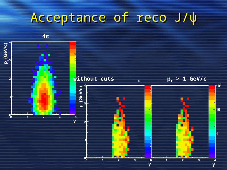
Acceptance of reco J/ψAcceptance of reco J/ψ
without cuts % pt > 1 GeV/c %
4π
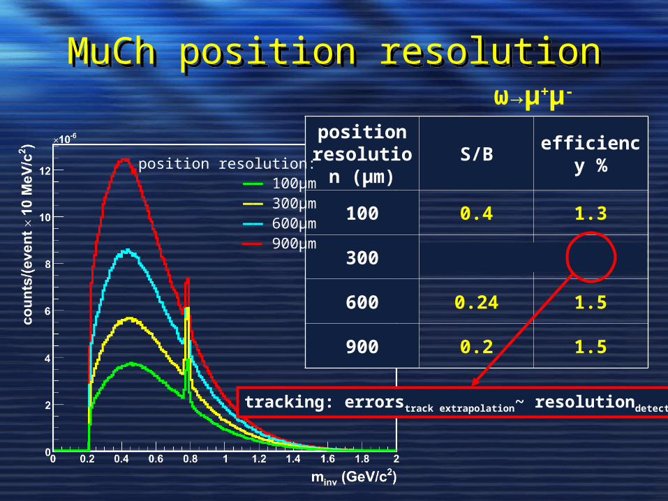
MuCh position resolutionMuCh position resolutionω→μ+μ-
position resolution
(μm)S/B
efficiency %
100 0.4 1.3
300 0.5 2.3
600 0.24 1.5
900 0.2 1.5
tracking: errorstrack extrapolation~ resolutiondetector
position resolution:—— 100μm—— 300μm—— 600μm—— 900μm
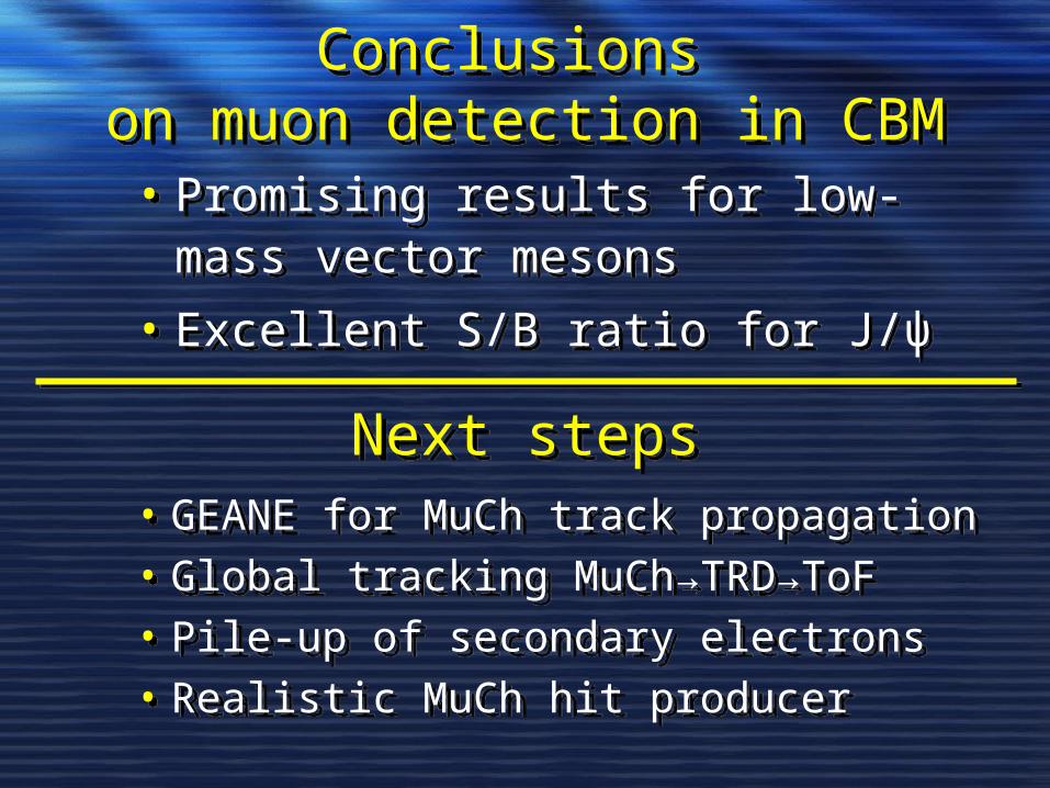
Next stepsNext steps• GEANE for MuCh track propagation
• Global tracking MuCh→TRD→ToF
• Pile-up of secondary electrons
• Realistic MuCh hit producer
• GEANE for MuCh track propagation
• Global tracking MuCh→TRD→ToF
• Pile-up of secondary electrons
• Realistic MuCh hit producer
Conclusions on muon detection in CBM
Conclusions on muon detection in CBM• Promising results for low-mass vector
mesons
• Excellent S/B ratio for J/ψ
• Promising results for low-mass vector mesons
• Excellent S/B ratio for J/ψ
Thank you for your attention!Thank you for your attention!