New Metrics in Voltage Partitioning with Application to Floorplanning

New Metrics in Voltage Partitioning with Application to Floorplanning

Shiyan HuDept of Electrical and Computer Engineering

Michigan Technological University

1

Peak Power Density Driven Voltage Partitioning

Introduction1

The Algorithm2

Conclusion4

Experimental Results3

2

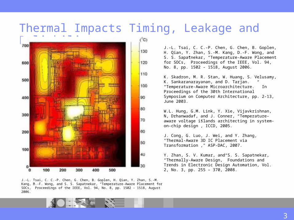
Thermal Impacts Timing, Leakage and Reliability

J.-L. Tsai, C. C.-P. Chen, G. Chen, B. Goplen, H. Qian, Y. Zhan, S.-M. Kang, D.-F. Wong, and S. S. Sapatnekar, “Temperature-Aware Placement for SOCs,” Proceedings of the IEEE, Vol. 94, No. 8, pp. 1502 - 1518, August 2006.

K. Skadron, M. R. Stan, W. Huang, S. Velusamy, K. Sankaranarayanan, and D. Tarjan. “Temperature-Aware Microarchitecture.” In Proceedings of the 30th International Symposium on Computer Architecture, pp. 2-13, June 2003.

W.L. Hung, G.M. Link, Y. Xie, Vijavkrishnan, N, Drhanwadaf, and J. Conner, “Temperature-aware voltage islands architecting in system-on-chip design”, ICCD, 2005.

J. Cong, G. Luo, J. Wei, and Y. Zhang, "Thermal-Aware 3D IC Placement via Transformation ," ASP-DAC, 2007.

Y. Zhan, S. V. Kumar, and S. S. Sapatnekar, “Thermally-Aware Design,” Foundations and Trends in Electronic Design Automation, Vol. 2, No. 3, pp. 255 – 370, 2008.

J.-L. Tsai, C. C.-P. Chen, G. Chen, B. Goplen, H. Qian, Y. Zhan, S.-M. Kang, D.-F. Wong, and S. S. Sapatnekar, “Temperature-Aware Placement for SOCs,” Proceedings of the IEEE, Vol. 94, No. 8, pp. 1502 - 1518, August 2006.

3

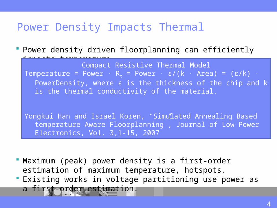
Power Density Impacts Thermal

Power density driven floorplanning can efficiently impacts temperature.

Maximum (peak) power density is a first-order estimation of maximum temperature, hotspots.

Existing works in voltage partitioning use power as a first-order estimation.

Compact Resistive Thermal ModelTemperature = Power Rt = Power ɛ/(k Area) = (ɛ/k) PowerDensity, where

ɛ is the thickness of the chip and k is the thermal conductivity of the material.

Yongkui Han and Israel Koren, “Simulated Annealing Based temperature Aware Floorplanning”, Journal of Low Power Electronics, Vol. 3,1-15, 2007

4

Previous Voltage Partitioning Works Do Not Consider Peak Power Density [1] Z. Gu, Y. Yang, J. Wang, R. Dick, and L. Shang, “Taphs: thermal-

aware unified physical-level and high-level synthesis,” ASPDAC, pp. 879 – 885, 2006.

[2] H.-Y. Liu, W.-P. Lee, and Y.-W. Chang, “A provably good approximation algorithm for power optimization using multiple supply voltages,” DAC, pp. 887 – 890, 2007.

[3] Tao Lin, Sheqin Dong, Bei Yu, Song Chen, and Satoshi Goto: A revisit to voltage partitioning problem. GLSVLSI, pp.115 –118, 2010.

5

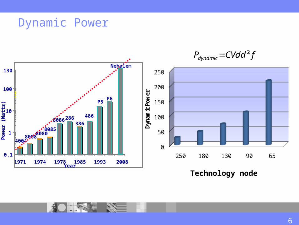
Dynamic Power

Technology node

0

50

100

150

200

250

250 180 130 90 65D

ynam

ic P

ower

fCVddPdynamic2

P6

486

3862868086

80858080

80084004

0.1

1

10

100

1971 1974 1978 1985 1993 2008Year

Po

we

r (W

att

s)

130Nehalem

P5

6

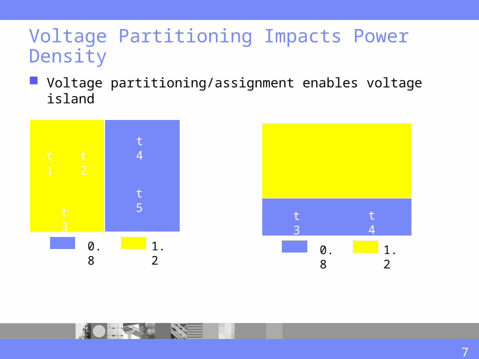
Voltage Partitioning Impacts Power Density

Voltage partitioning/assignment enables voltage island

0.8 1.2

t1 t2

t3

t4

t5

0.8 1.2

t1 t2

t3 t4

t5

7

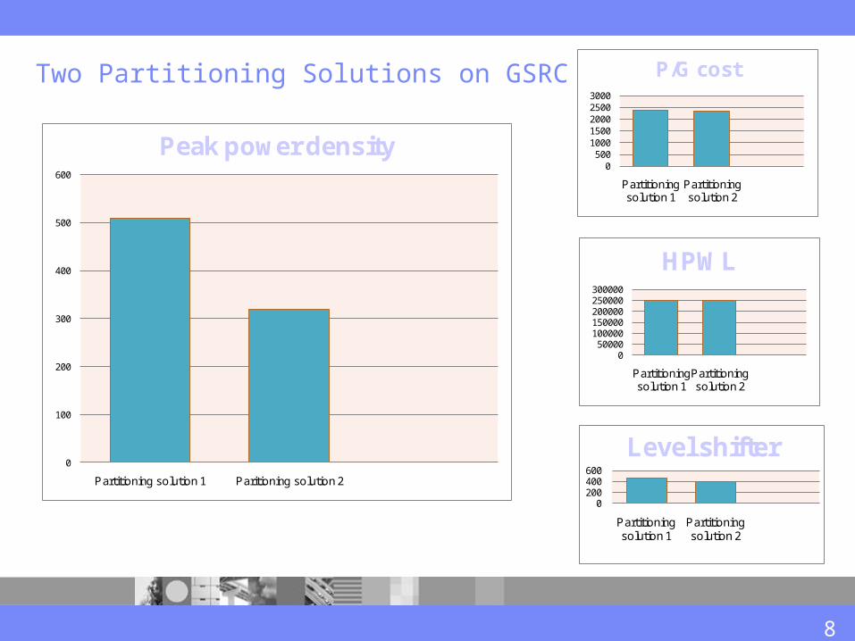
Two Partitioning Solutions on GSRC n100

0

100

200

300

400

500

600

Partitioning solution 1 Paritioning solution 2

Peak power density

0200400600

Partitioning solution 1


Level shifter

0500

10001500200025003000



P/G cost

050000

100000150000200000250000300000



HPWL

8

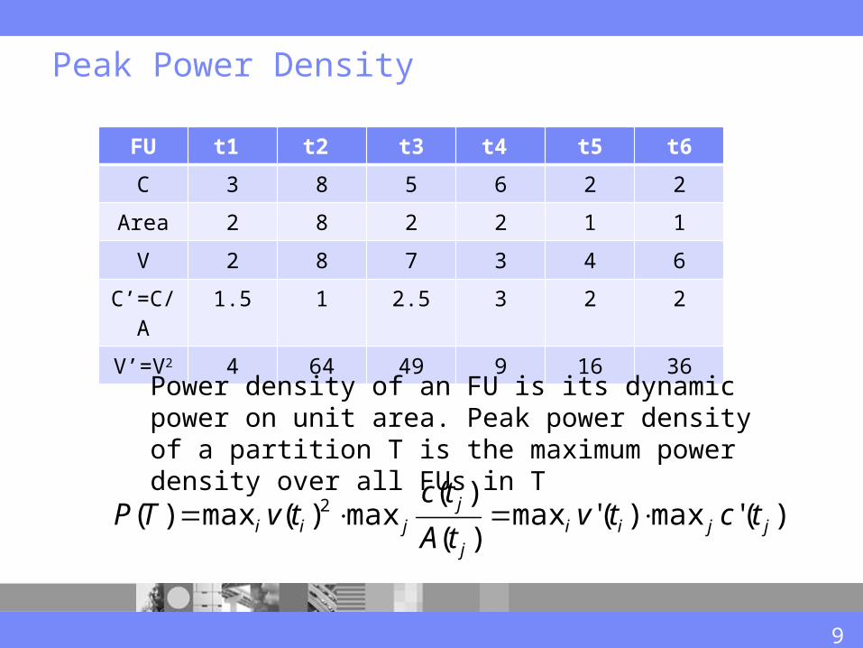
Peak Power Density

FU t1 t2 t3 t4 t5 t6

C 3 8 5 6 2 2

Area 2 8 2 2 1 1

V 2 8 7 3 4 6

C’=C/A 1.5 1 2.5 3 2 2

V’=V2 4 64 49 9 16 36

)('max)('max)(

)(max)(max)( 2

jjiij

jjii tctvtA

tctvTP

Power density of an FU is its dynamic power on unit area. Peak power density of a partition T is the maximum power density over all FUs in T

9

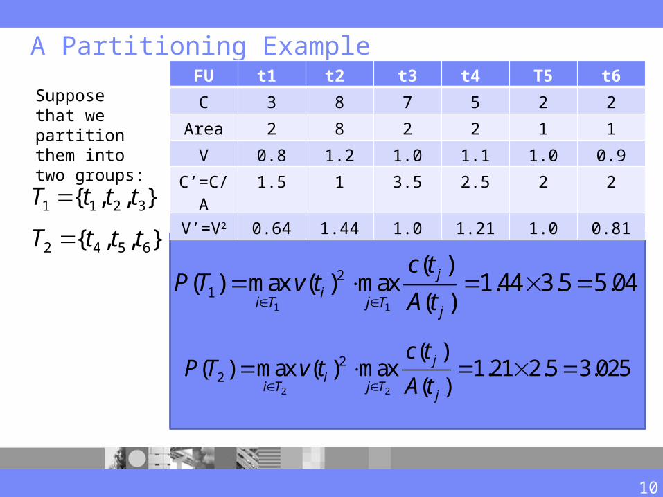
A Partitioning Example

Suppose that we partition them into two groups:

},,{ 3211 tttT

},,{ 6542 tttT

1 1

21

( )( ) max ( ) max 1.44 3.5 5.04

( )j

ii T j T

j

c tP T v t

A t

2 2

22

( )( ) max ( ) max 1.21 2.5 3.025

( )j

ii T j T

j

c tP T v t

A t

FU t1 t2 t3 t4 T5 t6

C 3 8 7 5 2 2

Area 2 8 2 2 1 1

V 0.8 1.2 1.0 1.1 1.0 0.9

C’=C/A 1.5 1 3.5 2.5 2 2

V’=V2 0.64 1.44 1.0 1.21 1.0 0.81

10

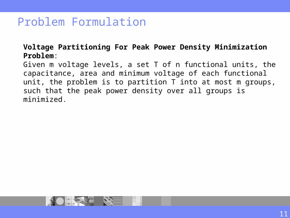
Problem Formulation

Voltage Partitioning For Peak Power Density Minimization Problem: Given m voltage levels, a set T of n functional units, the capacitance, area and minimum voltage of each functional unit, the problem is to partition T into at most m groups, such that the peak power density over all groups is minimized.

11

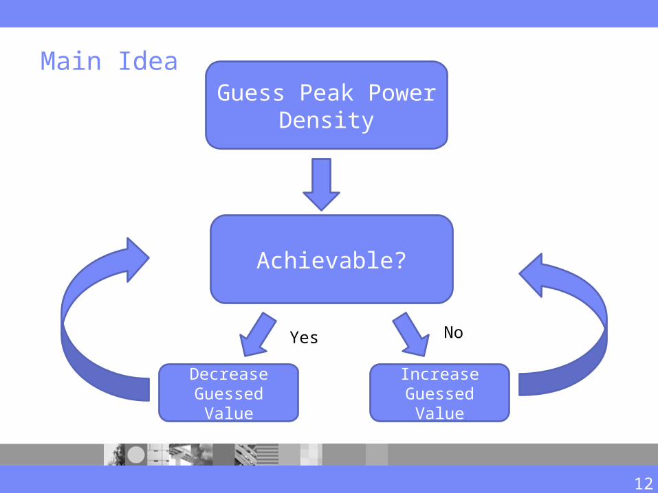
Main IdeaGuess Peak Power

Density

Achievable?

Decrease Guessed Value

Increase Guessed Value

Yes No

12

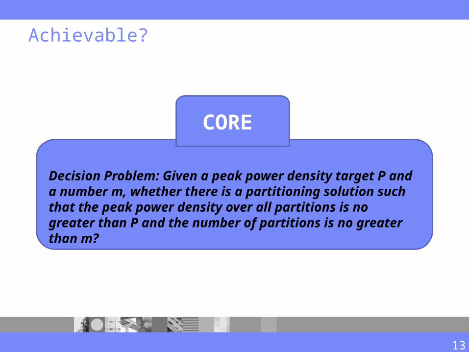
Achievable?

Decision Problem: Given a peak power density target P and a number m, whether there is a partitioning solution such that the peak power density over all partitions is no greater than P and the number of partitions is no greater than m?

CORE

13

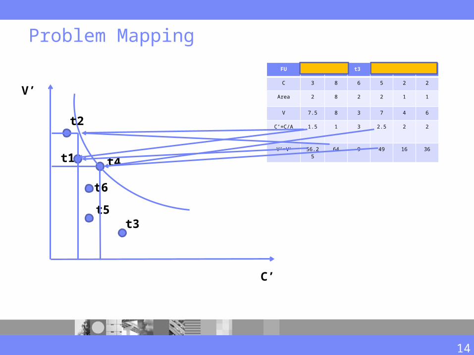
Problem Mapping

FU t1 t2 t3 T4 t5 t6

C 3 8 6 5 2 2

Area 2 8 2 2 1 1

V 7.5 8 3 7 4 6

C’=C/A 1.5 1 3 2.5 2 2

V’=V2 56.25 64 9 49 16 36

C’

V’

t1

t2

t4

t3t5

t6

14

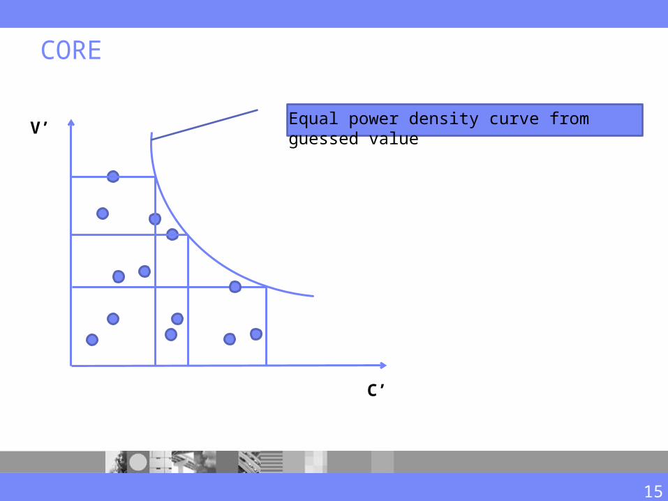
CORE

Equal power density curve from guessed value

C’

V’

15

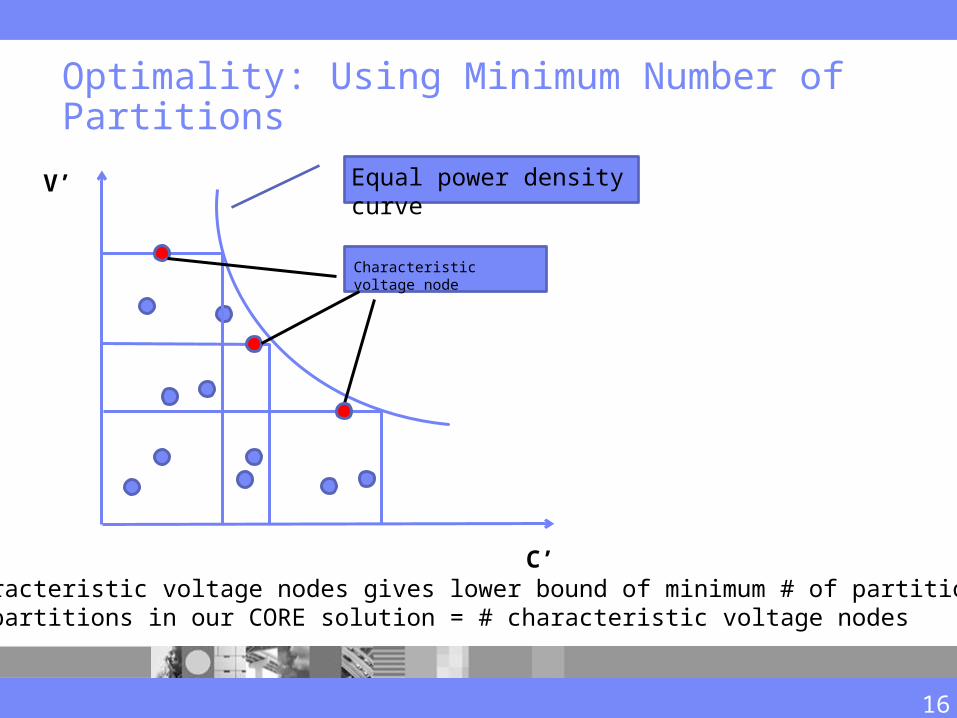
Optimality: Using Minimum Number of Partitions

Equal power density curve

C’

V’

Characteristic voltage node

16

# characteristic voltage nodes gives lower bound of minimum # of partitions# of partitions in our CORE solution = # characteristic voltage nodes

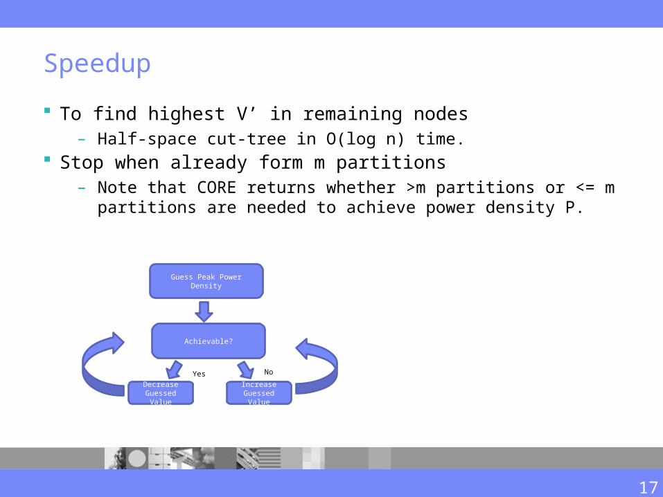
Speedup

To find highest V’ in remaining nodes– Half-space cut-tree in O(log n) time.

Stop when already form m partitions– Note that CORE returns whether >m partitions or <= m partitions are

needed to achieve power density P.

Guess Peak Power Density

Achievable?

Decrease Guessed

Value

Increase Guessed

Value

Yes No

17

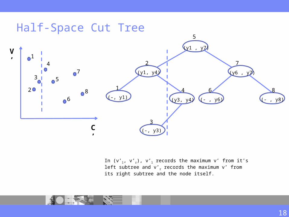
Half-Space Cut Tree

1

2

3

4

57

68

C’

V’

(-, y3)

3

1

2

4 6 8

7

5

(y3, y4)(-, y1)

(y1, y4)

(- , y6) (- , y8)

(y6 , y7)

(y1 , y7)

In (v’l, v’r), v’l records the maximum v’ from it’s left subtree and v’r records the maximum v’ from its right subtree and the node itself.

18

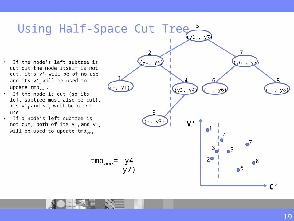
Using Half-Space Cut Tree

tmpvmax= 0max (y4, 0)

(-, y3)

3

1

2

4 6 8

7

5

(y3, y4)(-, y1)

(y1, y4)

(- , y6) (- , y8)

(y6 , y7)

(y1 , y7)

• If the node’s left subtree is cut but the node itself is not cut, it’s v’l will be of no use and its v’r will be used to update tmpvmax.

• If the node is cut (so its left subtree must also be cut), its v’l and v’r will be of no use.

• If a node’s left subtree is not cut, both of its v’l and v’r will be used to update tmpvmax

y4max (y4, y7)y4

1

2

3

4

57

68

C’

V’

19

CORE Theorem

Theorem 1: Given a set of T with n functional units, a power density target P and a number m, deciding whether there is a partitioning solution such that the peak power density over all partitions is no greater than P and the number of partitions is no greater than m can be performed in O(mlog n) time, excluding the O(nlog n) preprocessing time.

20

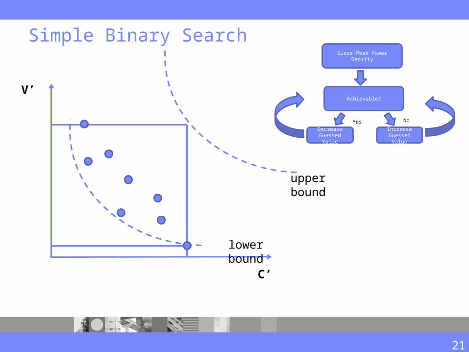
C’

V’

lower bound

upper bound

Guess Peak Power Density

Achievable?

Decrease Guessed

Value

Increase Guessed

Value

Yes No

Simple Binary Search

21

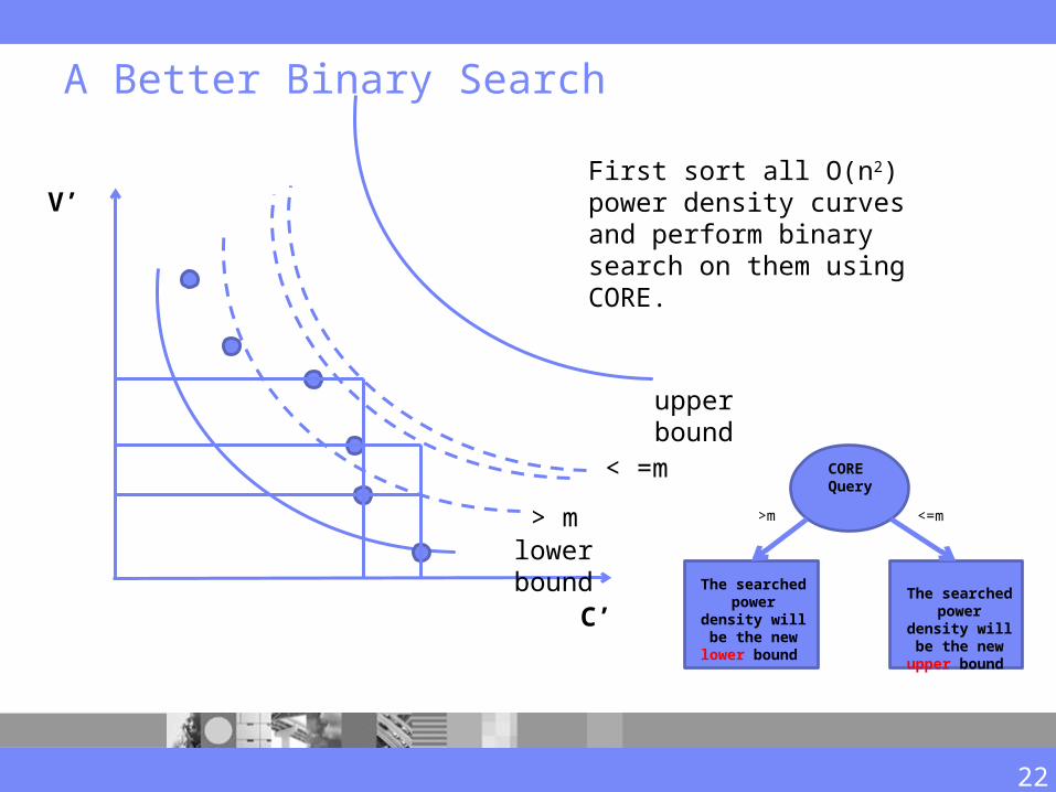
A Better Binary Search

C’

V’

lower bound

upper bound

First sort all O(n2) power density curves and perform binary search on them using CORE.

< =m

> m

CORE Query

>m <=m

The searched power density will be the new lower bound

The searched power density will be the new upper bound

22

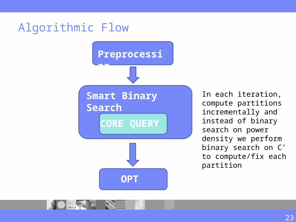
Algorithmic Flow

OPT

Smart Binary Search

Preprocessing

CORE QUERY

In each iteration, compute partitions incrementally and instead of binary search on power density we perform binary search on C’ to compute/fix each partition

23

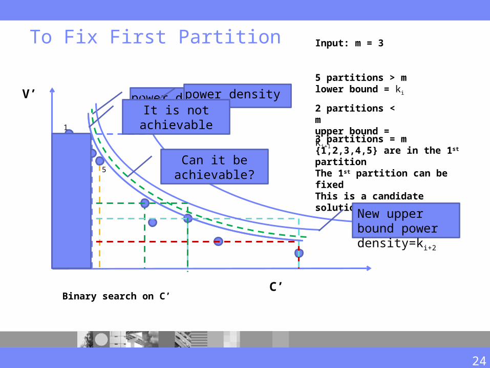
To Fix First Partition

C’

V’

Input: m = 3

5 partitions > mlower bound = ki

3 partitions = m{1,2,3,4,5} are in the 1st partitionThe 1st partition can be fixedThis is a candidate solution.

power density =ki2 partitions < mupper bound = ki+1

power density =ki+1

New upper bound power density=ki+2

Binary search on C’

1

2

3

4

5Can it be

achievable?

24

It is not achievable

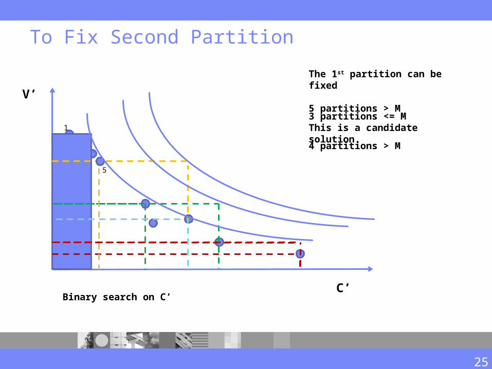
To Fix Second Partition

C’

V’


1

2

3

4

5

The 1st partition can be fixed

5 partitions > M

3 partitions <= MThis is a candidate solution.

4 partitions > M

25

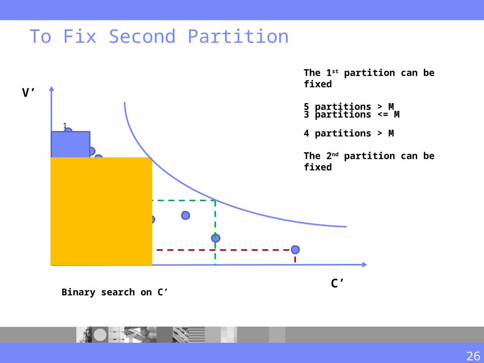
To Fix Second Partition

C’

V’


1

2

3

4

5

The 1st partition can be fixed

5 partitions > M

3 partitions <= M

4 partitions > M

The 2nd partition can be fixed

26

C’

V’


1

2

3

4

5

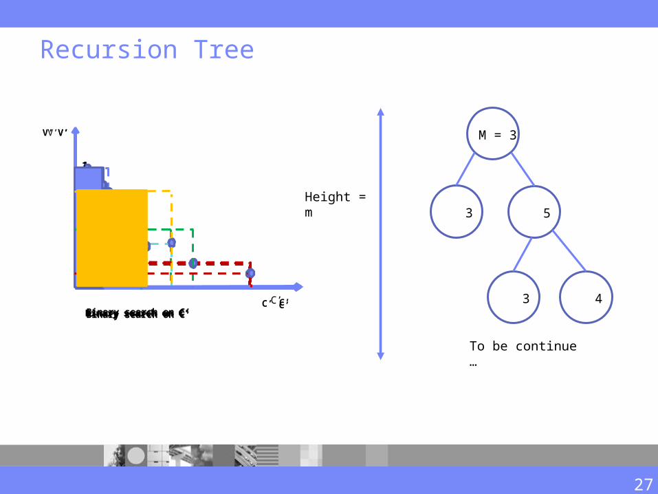
M = 3

3 5

3 4C’

V’


1

2

3

4

5

C’

V’


1

2

3

4

5

C’

V’


1

2

3

4

5 Height = m

To be continue …

Recursion Tree

27

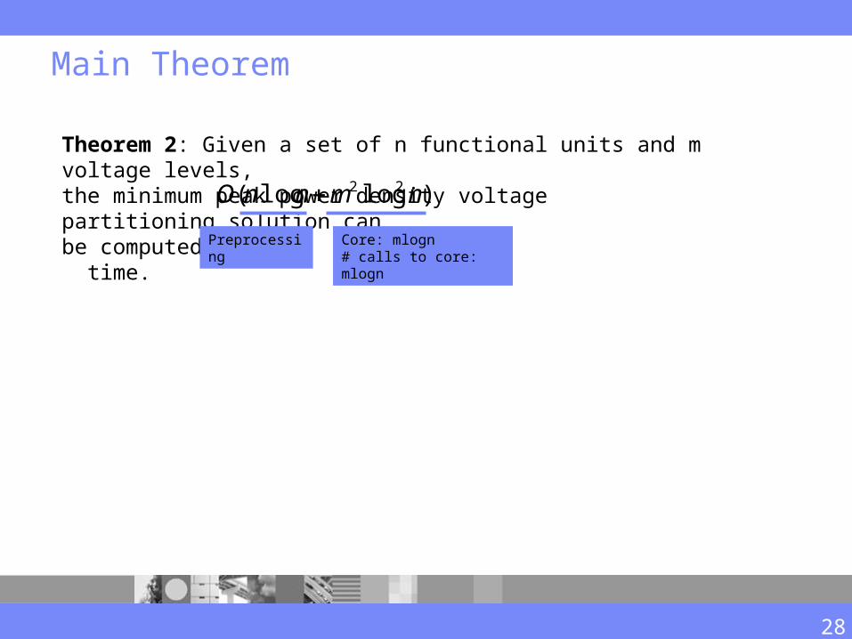
Main Theorem

Theorem 2: Given a set of n functional units and m voltage levels,the minimum peak power density voltage partitioning solution canbe computed in time.)loglog( 22 nmnnO

Preprocessing Core: mlogn# calls to core: mlogn

28

Experimental Setup

The algorithm is tested on a machine with a quad-core CPU at 2.4 GHz and 8G memory.

Randomly generated testcases whose sizes are from 100K to 1M. Compare to a natural greedy algorithm which iteratively assigns a

functional unit to the partition such that the power density can be minimized in this iteration.

29

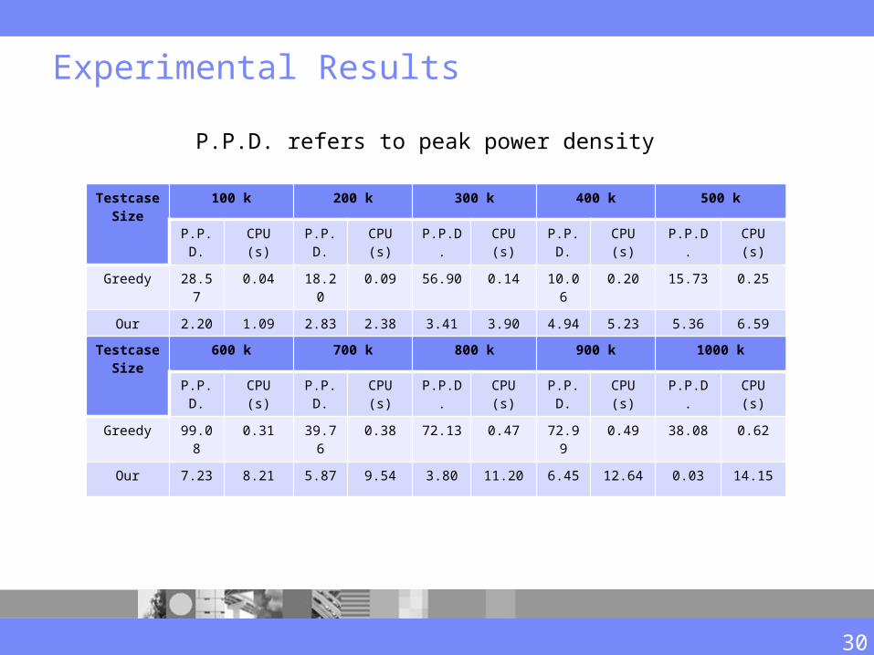
Experimental Results

TestcaseSize

100 k 200 k 300 k 400 k 500 k

P.P.D. CPU (s) P.P.D. CPU (s)

P.P.D. CPU (s)

P.P.D. CPU (s)

P.P.D. CPU (s)

Greedy 28.57 0.04 18.20 0.09 56.90 0.14 10.06 0.20 15.73 0.25

Our 2.20 1.09 2.83 2.38 3.41 3.90 4.94 5.23 5.36 6.59

TestcaseSize

600 k 700 k 800 k 900 k 1000 k

P.P.D. CPU (s) P.P.D. CPU (s)

P.P.D. CPU (s)

P.P.D. CPU (s)

P.P.D. CPU (s)

Greedy 99.08 0.31 39.76 0.38 72.13 0.47 72.99 0.49 38.08 0.62

Our 7.23 8.21 5.87 9.54 3.80 11.20 6.45 12.64 0.03 14.15

P.P.D. refers to peak power density

30

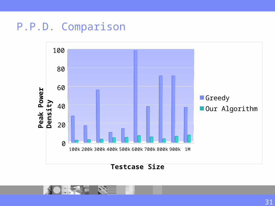
P.P.D. Comparison

100k 200k 300k 400k 500k 600k 700k 800k 900k 1M0

102030405060708090

100

GreedyOur Algorithm

Testcase Size

Pea

k P

ow

er D

ensi

ty

31

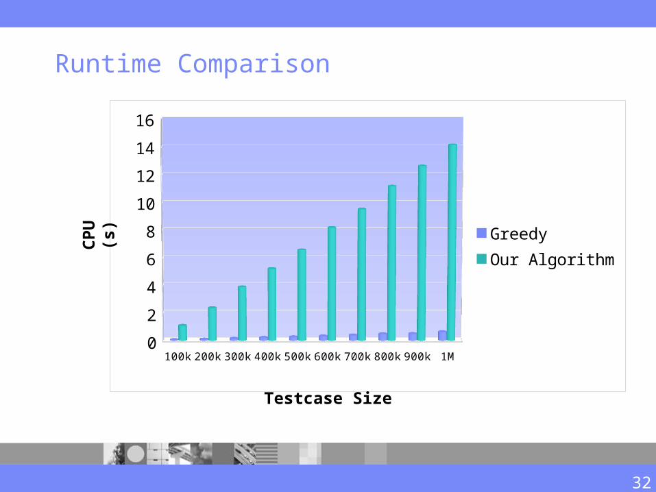
Runtime Comparison

100k 200k 300k 400k 500k 600k 700k 800k 900k 1M0

2

4

6

8

10

12

14

16

GreedyOur Algorithm

Testcase Size

CP

U (

s)

32

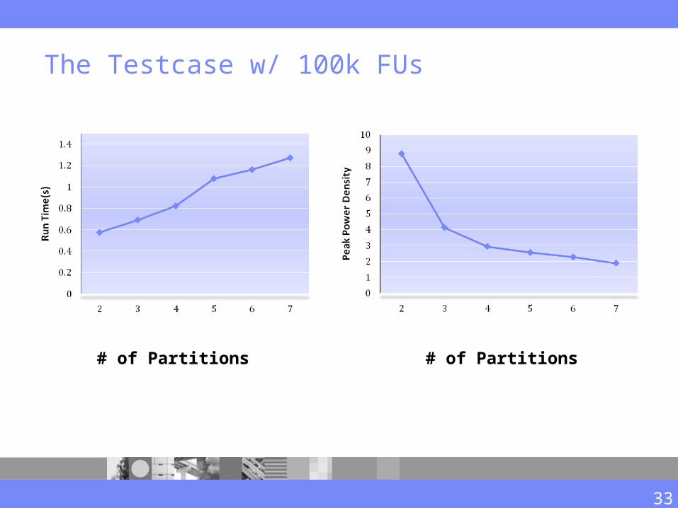
The Testcase w/ 100k FUs

# of Partitions # of Partitions

33

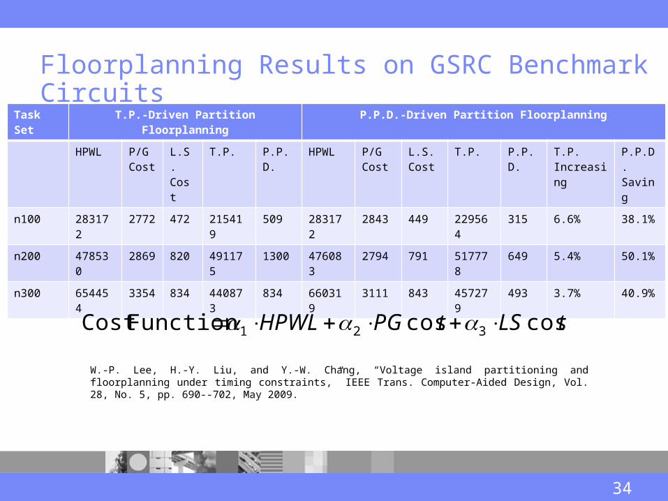
Floorplanning Results on GSRC Benchmark Circuits

Task Set T.P.-Driven Partition Floorplanning P.P.D.-Driven Partition Floorplanning

HPWL P/GCost

L.S. Cost

T.P. P.P.D. HPWL P/G Cost

L.S. Cost

T.P. P.P.D. T.P. Increasing

P.P.D. Saving

n100 283172 2772 472 215419 509 283172 2843 449 229564 315 6.6% 38.1%

n200 478530 2869 820 491175 1300 476083 2794 791 517778 649 5.4% 50.1%

n300 654454 3354 834 440873 834 660319 3111 843 457279 493 3.7% 40.9%

tLStPGHPWL coscos Function Cost 321

34

W.-P. Lee, H.-Y. Liu, and Y.-W. Chang, “Voltage island partitioning and floorplanning under timing constraints,” IEEE Trans. Computer-Aided Design, Vol. 28, No. 5, pp. 690--702, May 2009.

Conclusion for Peak Power Density Driven Voltage Partitioning This work proposes an efficient optimal voltage partitioning algorithm

for peak power density minimization, – The algorithm runs in O(nlogn + m2log2n) time, where n refers to the

number of functional units and m refers to the number of partitions.

– Experimental results on large testcases demonstrate that the proposed algorithm can achieve large amount of (about 9.7 X) reduction in peak power density compare to a natural greedy algorithm.

– Our algorithm needs only 14.15 seconds to optimize 1M functional units. Future work seeks to perform peak power density driven thermal

aware floorplanning.

35

Peak Power Driven Voltage Partitioning

Problem Formulation1

NP-Complete Proof2

The Algorithm3

Experimental Result4

5 Conclusion

36

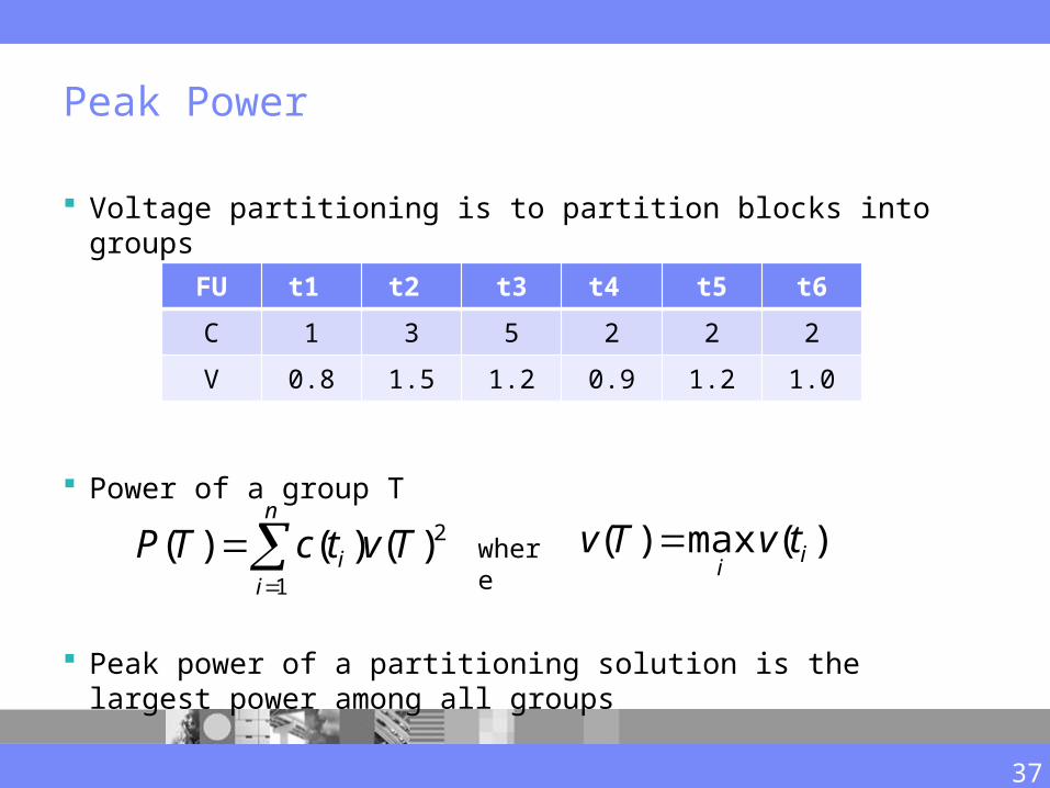
Peak Power

Voltage partitioning is to partition blocks into groups

Power of a group T

Peak power of a partitioning solution is the largest power among all groups


C 1 3 5 2 2 2

V 0.8 1.5 1.2 0.9 1.2 1.0

n

ii TvtcTP

1

2)()()( )(max)( ii

tvTv where

37

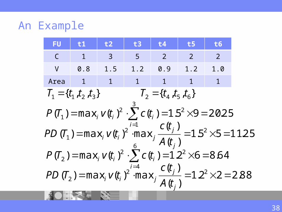
An Example

25.2095.1)()(max)( 23

1

21

iiii tctvTP

},,{ 3211 tttT },,{ 6542 tttT

64.862.1)()(max)( 26

4

22

iiii tctvTP


C 1 3 5 2 2 2

V 0.8 1.5 1.2 0.9 1.2 1.0

Area 1 1 1 1 1 1

25.1155.1)(

)(max)(max)( 22

1 j

jjii tA

tctvTPD

88.222.1)(

)(max)(max)( 22

2 j

jjii tA

tctvTPD

38

Power Balancing

t1 t2 t4t5

t3t6


C 1 3 5 2 2 2

V 0.8 1.5 1.2 0.9 1.2 1.0

t1 t2t4t5

t3t6

39

},,{ 5211 tttT },,{ 6432 tttT

46.2696.125.13 TP

},,,,{ 654311 tttttT }{ 22 tT

03.2475.628.17 TP

Pow

er

Partition 1 Partition 2

Pow

er


Why balancing?

We tend to obtain a solution that power for each partition is similar to each other while the maximum power is minimized. Thus, the total power of our solution is also small.In contrast, total power minimization ignores balancing and peak power minimization.

Voltage Island Shutdown

When all blocks in a voltage island are not in use, the entire island can be shutdown to reduce power.

40

Ciprian Seiculescu, Srinivasan Murali, Giovanni De Micheli, “NoC Topology Synthesis for Supporting Shutdown of Voltage Islands in SoCs,” DAC’09.

Ashoka Visweswara Sathanur, Luca Benini, Alberto Macii, Enrico Macii and Massimo Poncino, "Multiple power-gating domain (multi-VGND) architecture for improved leakage power reduction", ISLPED’08.

David E. Lackey, Paul S. Zuchowski, Thomas R. Bednar, Douglas W. Stout, Scott W. Gould and John M. Cohn, "Managing power and performance for System-on-Chip designs using Voltage Islands", ICCAD’02.

Qiang Ma and Evangeline F.Y. Young, Voltage Island-Driven Floorplanning, ICCAD’07.

Shutdown v.s. Peak Power Reduction

Previous works assume that the shutdown frequency for each voltage island is known.

– They design application specific floorplan good for known shutdown frequency

– Valid for some very specific applications

– Not valid for general applications

– Shutdown frequency depends on input data, which are quite difficult to predict. For example, whether the user will surf the internet more or watch DVD more is not known

41

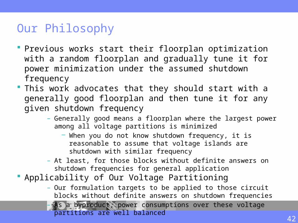
Our Philosophy

Previous works start their floorplan optimization with a random floorplan and gradually tune it for power minimization under the assumed shutdown frequency

This work advocates that they should start with a generally good floorplan and then tune it for any given shutdown frequency

– Generally good means a floorplan where the largest power among all voltage partitions is minimized

– When you do not know shutdown frequency, it is reasonable to assume that voltage islands are shutdown with similar frequency

– At least, for those blocks without definite answers on shutdown frequencies for general application

Applicability of Our Voltage Partitioning– Our formulation targets to be applied to those circuit blocks without definite

answers on shutdown frequencies– As a byproduct, power consumptions over these voltage partitions are well

balanced

42

Problem Formulation

Given a set of voltage levels, a set T of n functional units, the capacitance and minimum voltage of each functional unit, and a set of discrete voltage levels, to compute a voltage partitioning solution with m partitions such that the peak power over all partitions is minimized.

43

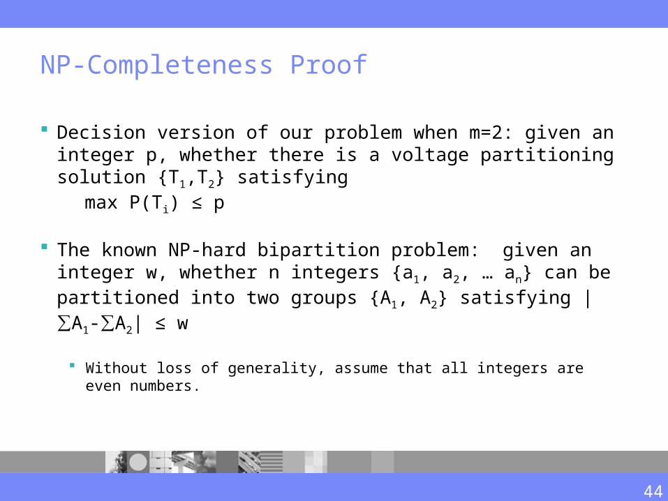
NP-Completeness Proof

Decision version of our problem when m=2: given an integer p, whether there is a voltage partitioning solution {T1,T2} satisfying

max P(Ti) ≤ p

The known NP-hard bipartition problem: given an integer w, whether n integers {a1, a2, … an} can be partitioned into two groups {A1, A2} satisfying |∑A1-∑A2| ≤ w

Without loss of generality, assume that all integers are even numbers.

44

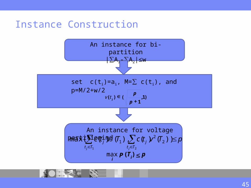
Instance Construction

An instance for voltage partitioning

set c(ti)=ai, M=∑ c(ti), and p=M/2+w/2

An instance for bi-partition|∑A1-∑A2|≤w

)1,1

()(+

Îp

ptvi

pTP ii£)(max

45

pTvtcTvtcTt

jTt

j

jj

))()(),()(max( 22

12

21

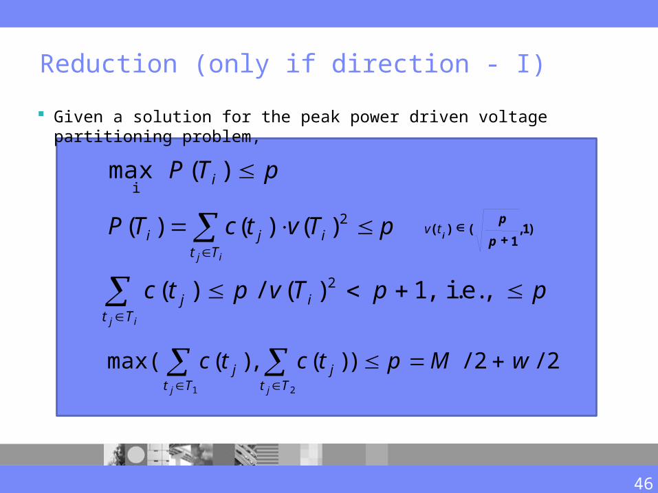
Reduction (only if direction - I)

Given a solution for the peak power driven voltage partitioning problem,

2( ) / ( ) 1, i.e., j i

j it T

c t p v T p p

2/2/))(,)(max(21

wMptctcTt

jTt

j

jj

pTvtcTP iTt

ji

ij

2)()()( )1,1

()(+

Îp

ptvi

46

pTP i )( maxi

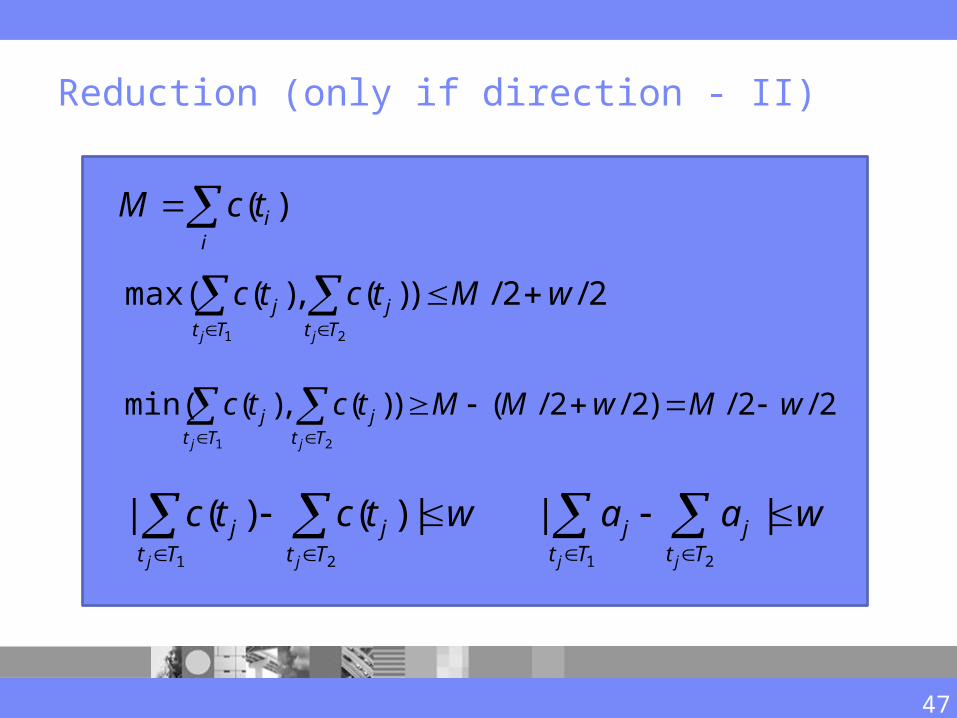
Reduction (only if direction - II))

2/2/)2/2/())(,)(min(21

wMwMMtctcTt

jTt

j

jj

i

itcM )(

wtctcTt

jTt

j

jj

|)()(|21

2/2/))(,)(max(21

wMtctcTt

jTt

j

jj

47

1 2

| |j j

j jt T t T

a a w

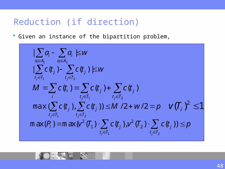
Reduction (if direction)

Given an instance of the bipartition problem,

wtctcTt

jTt

j

jj

|)()(|21

pwMtctcTt

jTt

j

jj

2/2/))(,)(max(21

1)( 2 iTv

48

21

)()()(Tt

jTt

ji

i

jj

tctctcM

waaAa Aa

ii

i i

||1 2

1 2

2 21 2max( ) max( ( ) ( ), ( ) ( ))

j j

i j jt T t T

P v T c t v T c t p

NP-Completeness Theorem

Theorem 1: The voltage partitioning for peak power minimization problem is NP-complete.

49

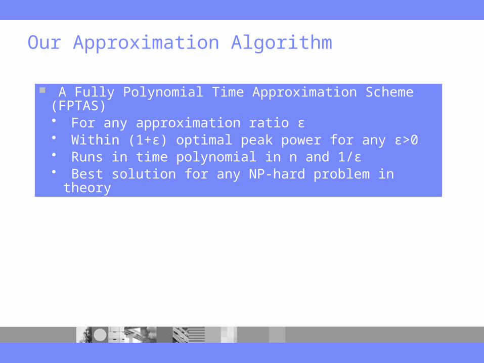
Our Approximation Algorithm

A Fully Polynomial Time Approximation Scheme (FPTAS)• For any approximation ratio ɛ • Within (1+ɛ) optimal peak power for any ɛ>0• Runs in time polynomial in n and 1/ɛ• Best solution for any NP-hard problem in theory

Naive Dynamic Programming

51


{t1} {--}

{--} {t1}

{t1 ,t2} {--}

{t2}{t1}

{t2} {t1}

{t1,t2}{--}

Exponential (mn) # Solutions

Needs speedup

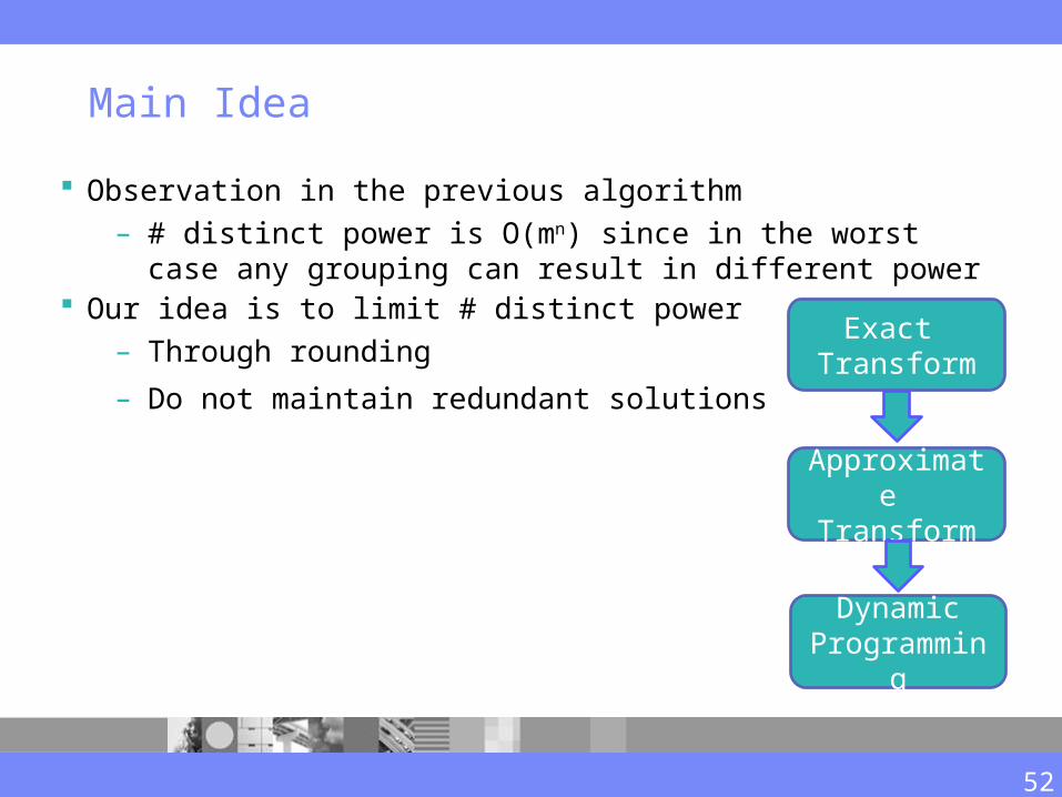
Main Idea

52

Exact Transform

Approximate Transform

Observation in the previous algorithm– # distinct power is O(mn) since in the worst case any grouping

can result in different power Our idea is to limit # distinct power

– Through rounding

– Do not maintain redundant solutions

Dynamic Programming

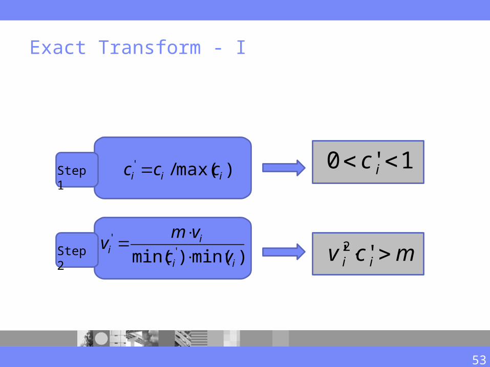
Exact Transform - I

mcv ii ''2

1'0 ic)max(/'iii ccc

)min()min( ''

ii

ii vc

vmv

Step 1

Step 2

53

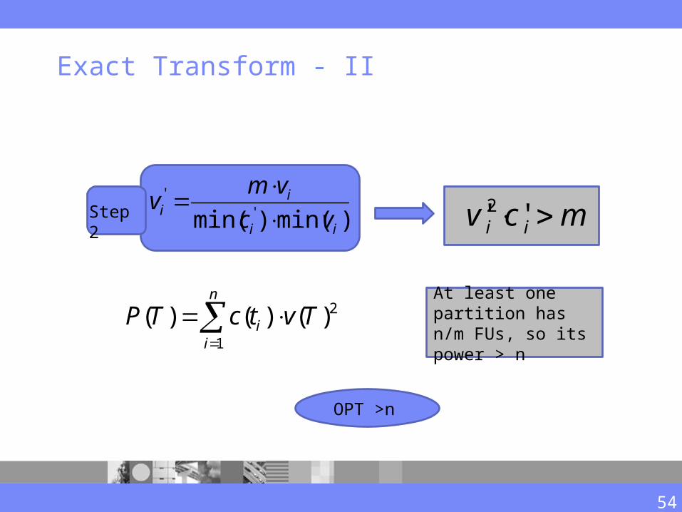
Exact Transform - II

mcv ii ''2)min()min( ''

ii

ii vc

vmv

Step 2

n

ii TvtcTP

1

2)()()(

OPT >n

At least one partition has n/m FUs, so its power > n

54

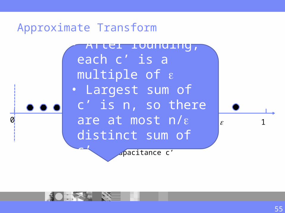
Approximate Transform

2 10 1

55

Capacitance c’

• After rounding, each c’ is a multiple of

• Largest sum of c’ is n, so there are at most n/ distinct sum of c’

New Dynamic Programming

Previously, # of solutions in tenth iteration = (# of solutions in nineth iteration) x m

56


{t1, t3, t5, t7, t8 } {t2 , t4, t6, t9, t10 }

{t1, t2, t3, t5, t7, t8 } {t4 , t6, t9, t10 }

{t1, t4, t7, t8 } {t2, t3, t5, t6, t9, t10 }

{t1, t3, t4 } {t2, t5, t6, t7, t8, t9, t10 }

{t1, t6, t7, t8 } {t2, t3, t4, t5, t9, t10 }

{t1, t9, t10} {t2, t3, t4, t5, t6, t7, t8}

{t1, t6, t7, t8 } {t2, t3, t4, t5, t9, t10 }

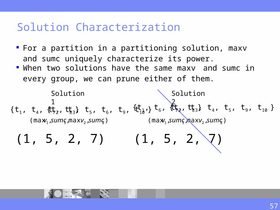
Solution Characterization

For a partition in a partitioning solution, maxv and sumc uniquely characterize its power.

When two solutions have the same maxv and sumc in every group, we can prune either of them.

57

(1, 5, 2, 7)

),max,,(max 2211 sumcvsumcv

Solution 1

(1, 5, 2, 7)


Solution 2

{t1, t6, t7, t8 } {t2, t3, t4, t5, t9, t10 }{t1, t4, t7, t8 } {t2, t3, t5, t6, t9, t10 }

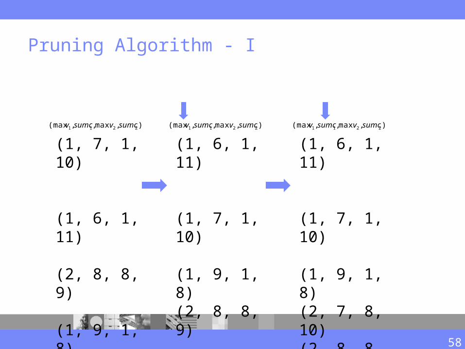
Pruning Algorithm - I

(1, 7, 1, 10) (1, 6, 1, 11) (2, 8, 8, 9) (1, 9, 1, 8) (2, 7, 8, 10) (2, 8, 8, 9)

),max,,(max 2211 sumcvsumcv ),max,,(max 2211 sumcvsumcv

(1, 6, 1, 11) (1, 7, 1, 10) (1, 9, 1, 8)(2, 8, 8, 9) (2, 7, 8, 10) (2, 8, 8, 9)


(1, 6, 1, 11) (1, 7, 1, 10) (1, 9, 1, 8)(2, 7, 8, 10) (2, 8, 8, 9) (2, 8, 8, 9)

58

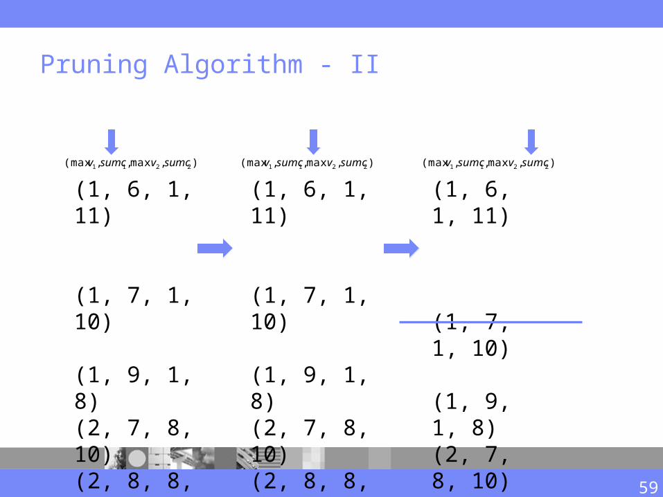
Pruning Algorithm - II

(1, 6, 1, 11) (1, 7, 1, 10) (1, 9, 1, 8)(2, 7, 8, 10) (2, 8, 8, 9) (2, 8, 8, 9)


(1, 6, 1, 11) (1, 7, 1, 10) (1, 9, 1, 8)(2, 7, 8, 10) (2, 8, 8, 9) (2, 8, 8, 9)


(1, 6, 1, 11) (1, 7, 1, 10) (1, 9, 1, 8)(2, 7, 8, 10) (2, 8, 8, 9) (2, 8, 8, 9)


59

Time Complexity

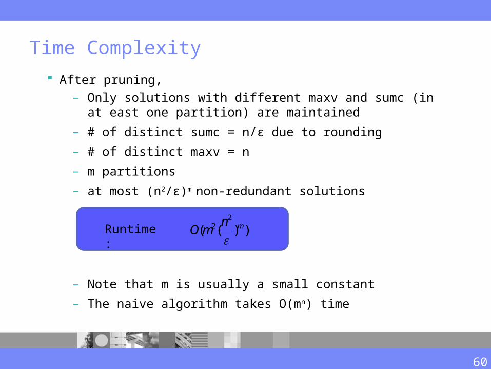
After pruning,

– Only solutions with different maxv and sumc (in at east one partition) are maintained

– # of distinct sumc = n/ε due to rounding

– # of distinct maxv = n

– m partitions

– at most (n2/ε)m non-redundant solutions

– Note that m is usually a small constant

– The naive algorithm takes O(mn) time

))((2

2 mnmO

Runtime :

60

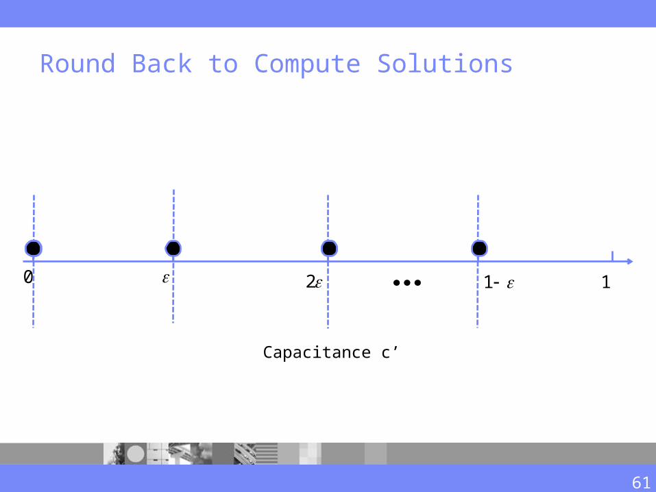
Round Back to Compute Solutions

2 10 1

61

Capacitance c’

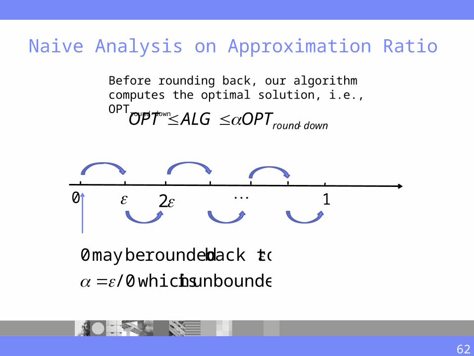
Naive Analysis on Approximation Ratio

downroundOPTALGOPT

0 1

62

2

unbounded is which /0

back to rounded bemay 0

Before rounding back, our algorithm computes the optimal solution, i.e., OPTround-down

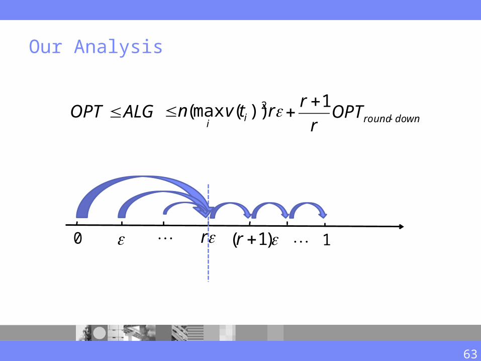
Our Analysis

ALGOPT

r )1( r0 1

63

downroundOPTr

r

1rtvn ii

2))(max(

Approximation Guarantee

rtvOPTOPTr

rALG i

i

2))(max(1

8))((max

1,

1

ii

tvrSet

OPTOPTALG )21()1( 4/14/1

OPT)'1(

64

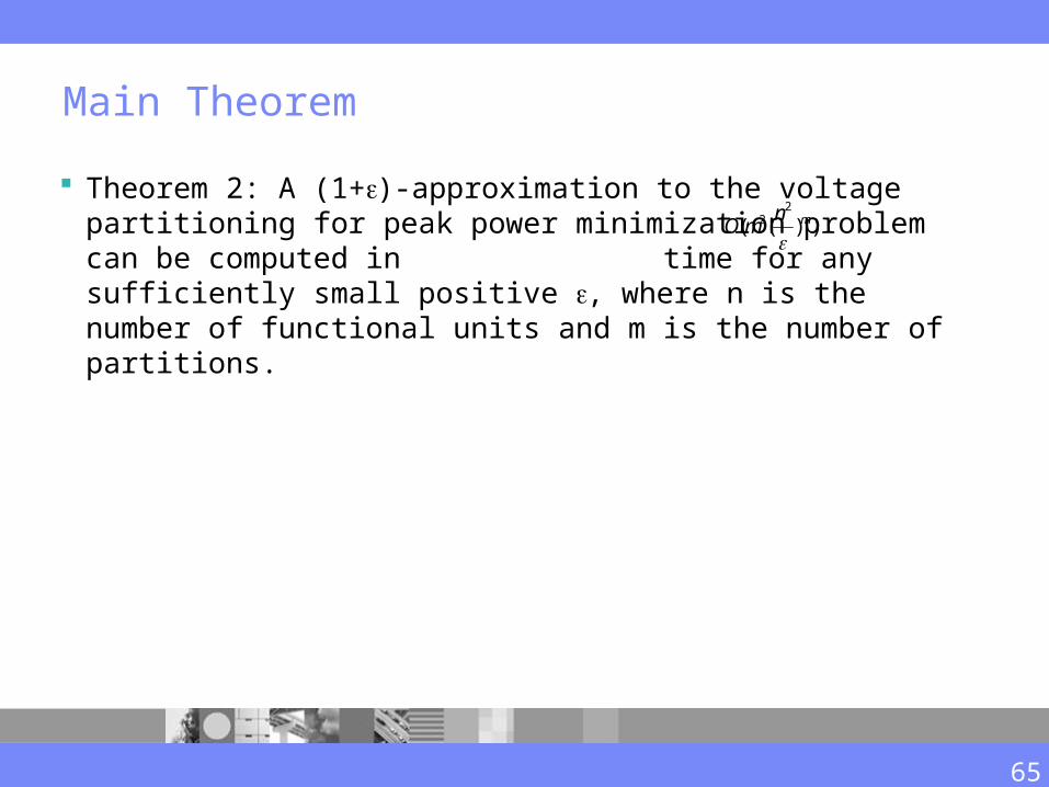
Main Theorem

Theorem 2: A (1+)-approximation to the voltage partitioning for peak power minimization problem can be computed in time for any sufficiently small positive , where n is the number of functional units and m is the number of partitions.

))((2

2 mnmO

65

Experimental Setup

The algorithm is tested on a machine with a dual-core CPU at 1.8 GHz and 2G memory.

The experiments are performed on a set of 10 randomly generated data flow graphs of various scales using TGFF.

For each testcase, the capacitances are randomly generated with means of 20pF. Five voltage levels are used in the technology library.

R. Dick, D. Rhodes, and W. Wolf, “TGFF: Task Graphs for Free,” Proceedings of the 6th International Workshop on Hardware/Software Codesign, pp. 97 – 101, 1998.

66

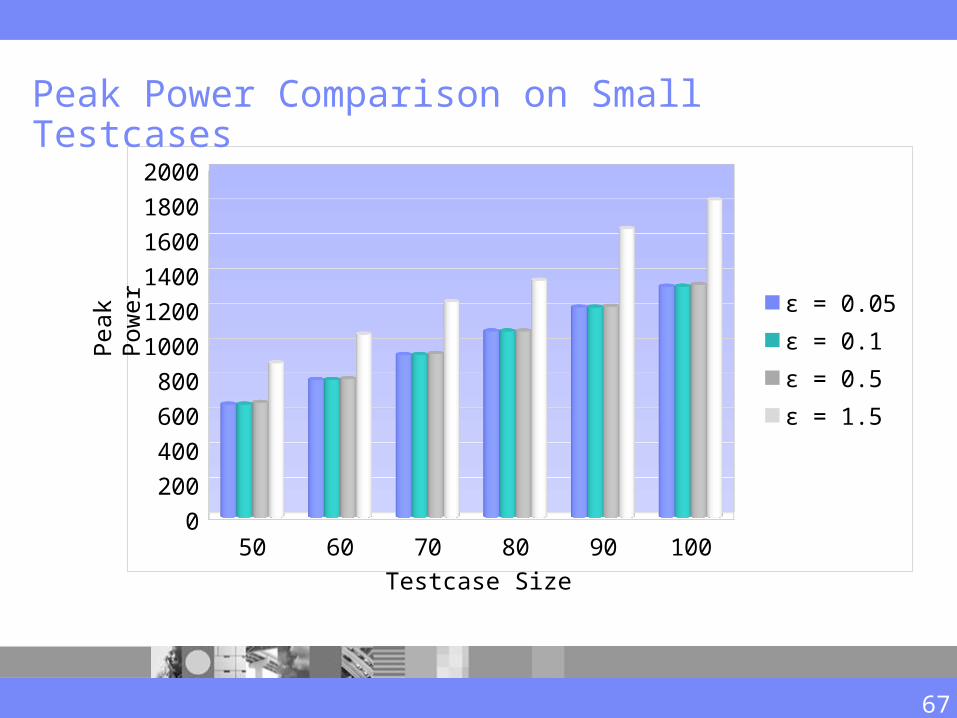
50 60 70 80 90 1000

200

400

600

800

1000

1200

1400

1600

1800

2000

ɛ = 0.05ɛ = 0.1ɛ = 0.5ɛ = 1.5

Peak Power Comparison on Small Testcases

Testcase Size

Pea

k P

ower

67

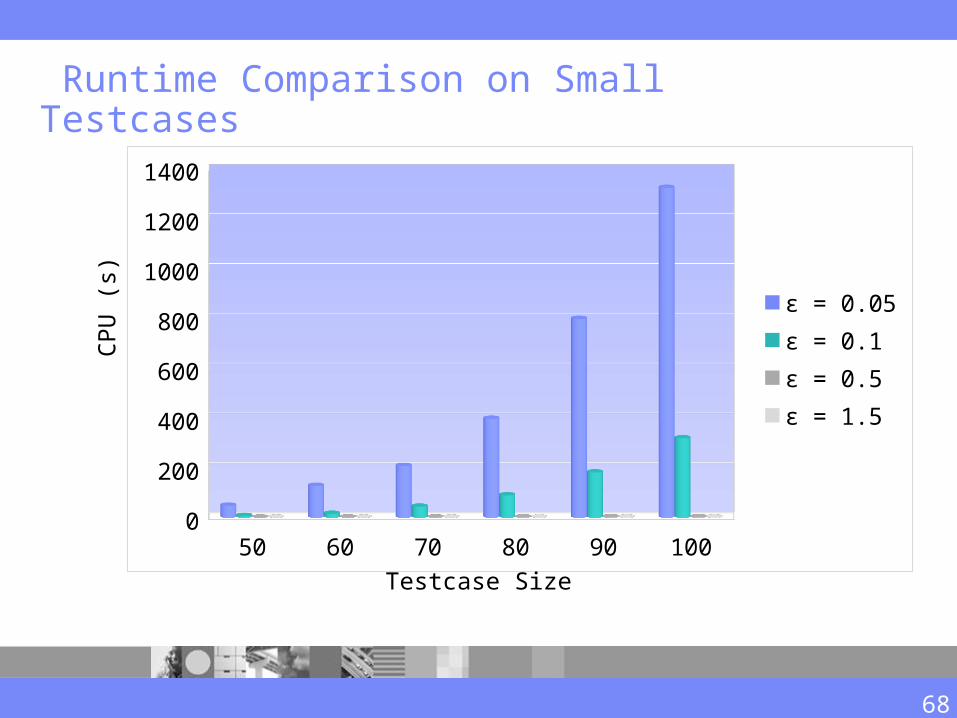
Runtime Comparison on Small Testcases

50 60 70 80 90 1000

200

400

600

800

1000

1200

1400

ɛ = 0.05ɛ = 0.1ɛ = 0.5ɛ = 1.5

Testcase Size

CP

U (

s)

68

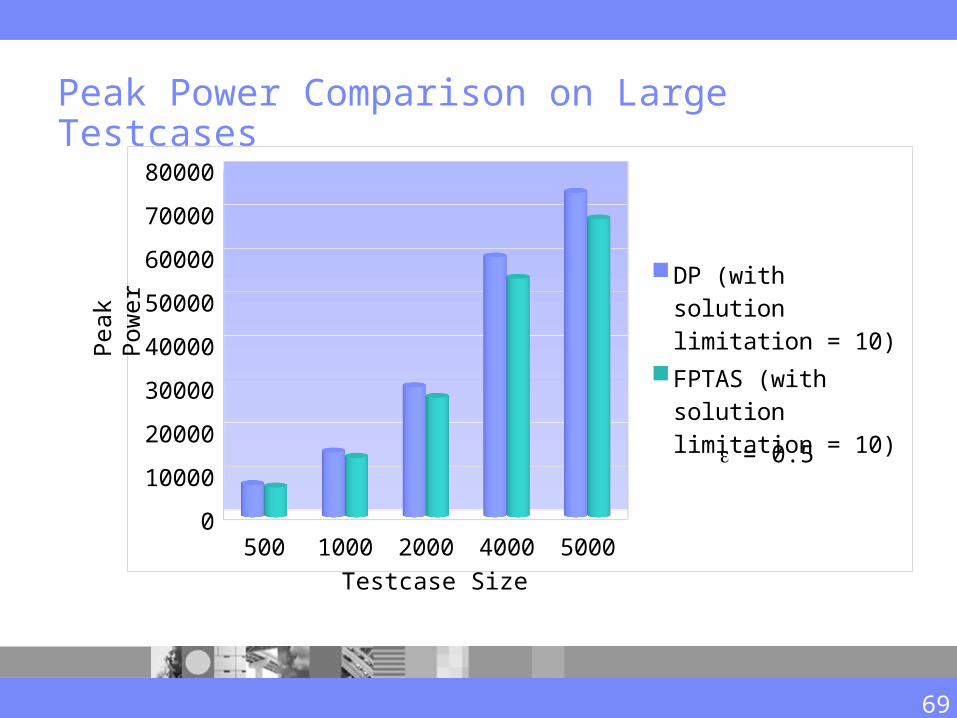
Peak Power Comparison on Large Testcases

500 1000 2000 4000 50000

10000

20000

30000

40000

50000

60000

70000

80000

DP (with solution limi-tation = 10)FPTAS (with solution limitation = 10)

Pea

k P

ower

69

Testcase Size

= 0.5

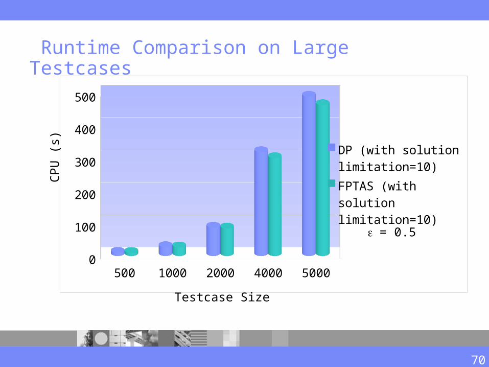
Runtime Comparison on Large Testcases

500 1000 2000 4000 50000

50100150200250300350400450500

DP (with solution limi-tation=10)FPTAS (with solution limitation=10)

CP

U (

s)

70

Testcase Size

= 0.5

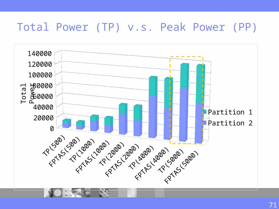
Total Power (TP) v.s. Peak Power (PP)

TP(500

)

FPTAS(500

)

TP(100

0)

FPTAS(100

0)

TP(200

0)

FPTAS(200

0)

TP(400

0)

FPTAS(400

0)

TP(500

0)

FPTAS(500

0)

0

20000

40000

60000

80000

100000

120000

140000

Partition 1Partition 2

Tota

l P

ower

71

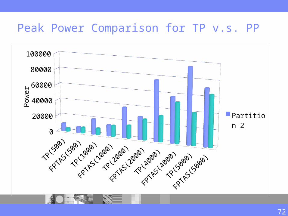
Peak Power Comparison for TP v.s. PPP

ower

72

TP(500

)

FPTAS(500

)

TP(100

0)

FPTAS(100

0)

TP(200

0)

FPTAS(200

0)

TP(400

0)

FPTAS(400

0)

TP(500

0)

FPTAS(500

0)

0

20000

40000

60000

80000

100000

Partition 2Partition 1

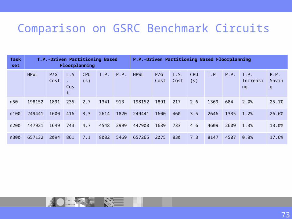
Comparison on GSRC Benchmark Circuits

Task set

T.P.-Driven Partitioning Based Floorplanning P.P.-Driven Partitioning Based Floorplanning

HPWL P/G Cost

L.S. Cost

CPU(s)

T.P. P.P. HPWL P/G Cost

L.S. Cost

CPU(s)

T.P. P.P. T.P.Increasing

P.P.Saving

n50 198152 1891 235 2.7 1341 913 198152 1891 217 2.6 1369 684 2.0% 25.1%

n100 249441 1600 416 3.3 2614 1820 249441 1600 460 3.5 2646 1335 1.2% 26.6%

n200 447921 1649 743 4.7 4548 2999 447900 1639 733 4.6 4609 2609 1.3% 13.0%

n300 657132 2094 861 7.1 8082 5469 657265 2075 830 7.3 8147 4507 0.8% 17.6%

73

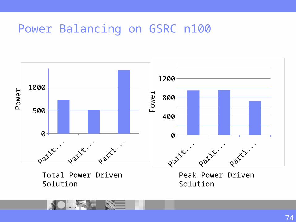
Power Balancing on GSRC n100

Parition 1

Parition 2

Partition 3

0200400600800

100012001400

Parition 1

Parition 2

Partition 3

0200400600800

100012001400

74

Pow

er

Pow

er

Total Power Driven Solution Peak Power Driven Solution

Conclusion for Peak Power Driven Voltage Partitioning The problem of voltage partitioning for peak power minimization is

proven to be NP-complete. An FPTAS algorithm is proposed to approximate the optimal solution

within a factor of 1 + ε in O(m2 (n2/ε)m) time for any sufficiently small positive ε, where n is the number of functional units and m is the number of partitions, which is a small constant in practice.

Our future work seeks to integrate the proposed peak power driven voltage partitioning with voltage islands shutdown techniques for power reduction.

75

Documents

New Metrics in Voltage Partitioning with Application to Floorplanning