Non linear studies on ALBA lattice

Zeus Martí

CELLS site

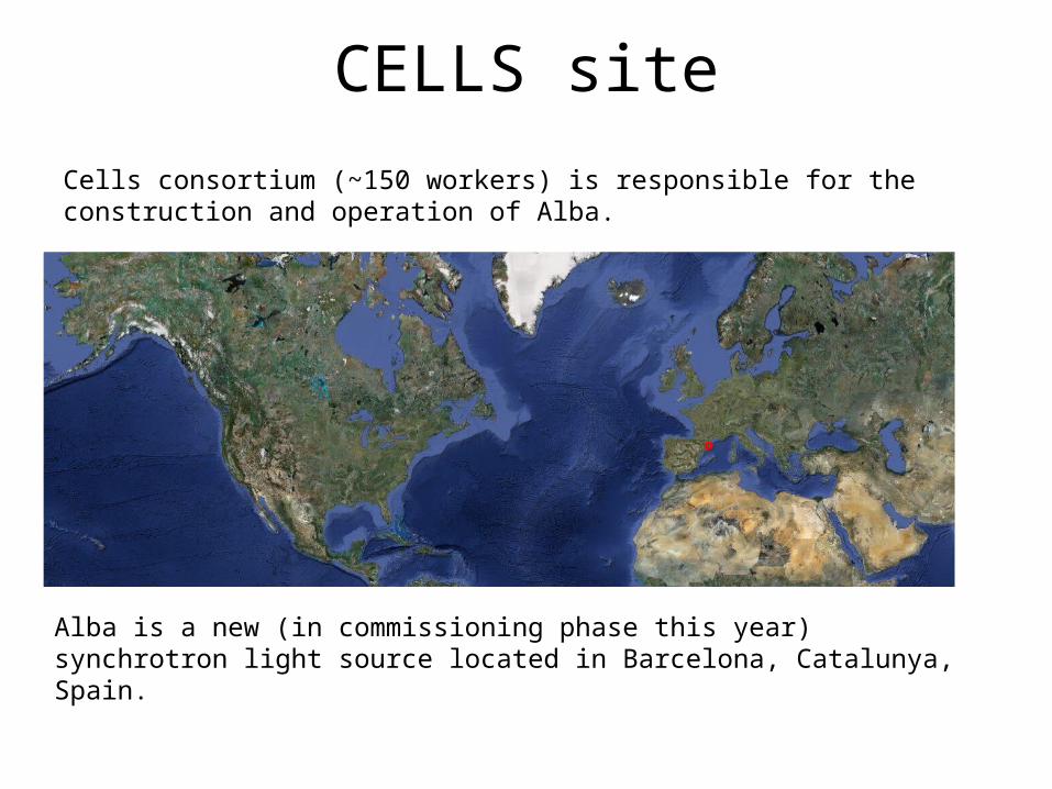
Alba is a new (in commissioning phase this year) synchrotron light source located in Barcelona, Catalunya, Spain.

Cells consortium (~150 workers) is responsible for the construction and operation of Alba.

Alba Lattice

Per

iodi

c S

ym.

Mirror S

ym.

Periodic Sym.

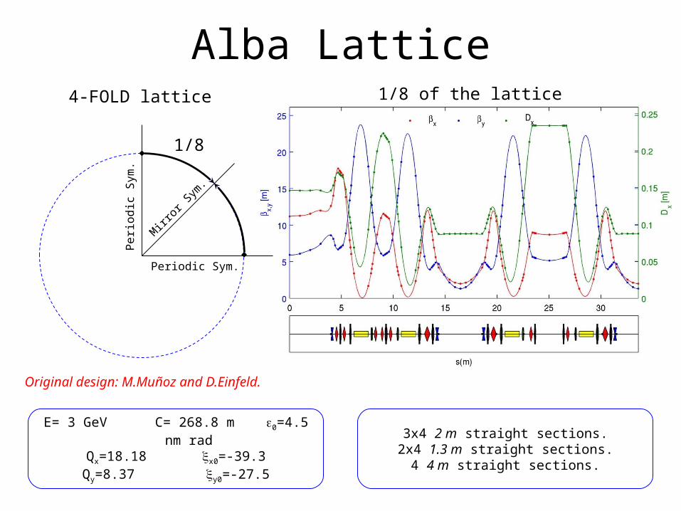
4-FOLD lattice 1/8 of the lattice

E= 3 GeV C= 268.8 m 0=4.5 nm radQx=18.18 x0=-39.3Qy=8.37 y0=-27.5

3x4 2 m straight sections.2x4 1.3 m straight sections.

4 4 m straight sections.

Original design: M.Muñoz and D.Einfeld.

1/8

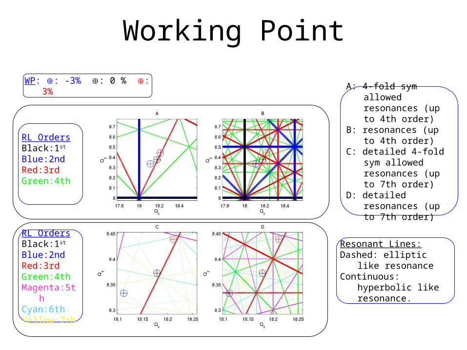
A: 4-fold sym allowed resonances (up to 4th order)

B: resonances (up to 4th order)

C: detailed 4-fold sym allowed resonances (up to 7th order)

D: detailed resonances (up to 7th order)

RL OrdersBlack:1st

Blue:2ndRed:3rdGreen:4thMagenta:5thCyan:6thYellow:7th

WP: : -3% : 0 % : 3%

RL OrdersBlack:1st

Blue:2ndRed:3rdGreen:4th

Resonant Lines:Dashed: elliptic like

resonanceContinuous: hyperbolic like

resonance.

Working Point

Tune shifts

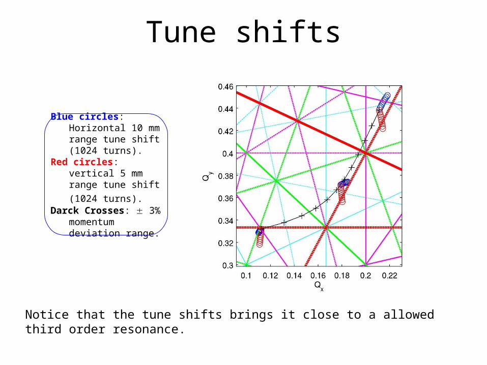
Blue circles: Horizontal 10 mm range tune shift (1024 turns).

Red circles: vertical 5 mm range tune shift (1024 turns).

Darck Crosses: 3% momentum deviation range.

Notice that the tune shifts brings it close to a allowed third order resonance.

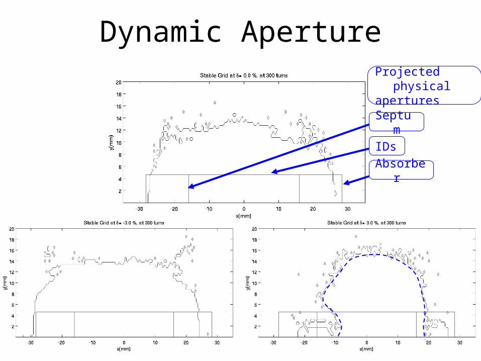
Projected physicalapertures

Septum

IDs

Absorber

Dynamic Aperture

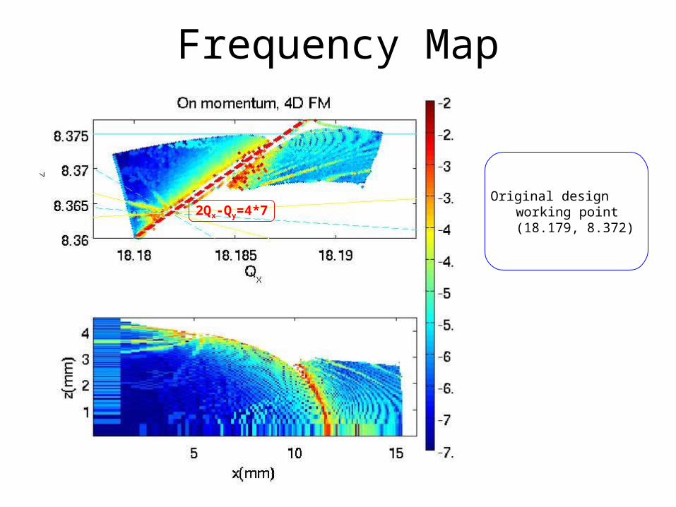
2Qx-Qy=4*7

Frequency Map

Original design working point (18.179, 8.372)

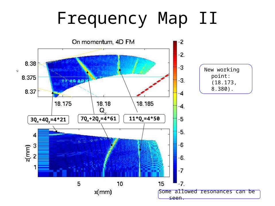
7Qx+2Qy=4*613Qx+4Qy=4*21 11*Qx=4*50

Some allowed resonances can be seen.

New working point: (18.173, 8.380).

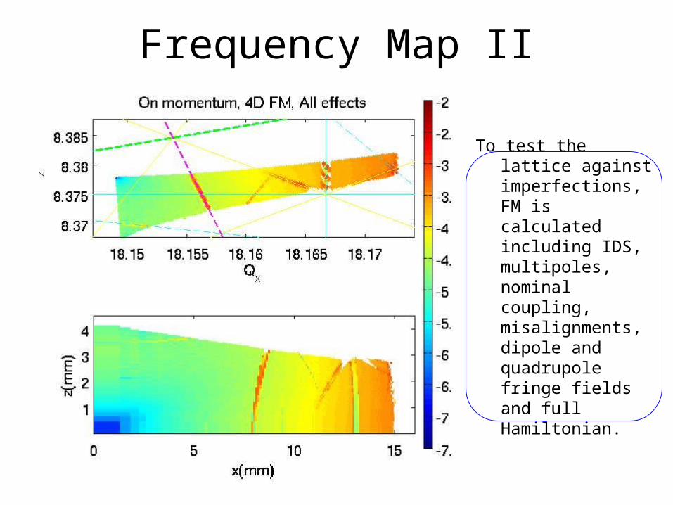
Frequency Map II

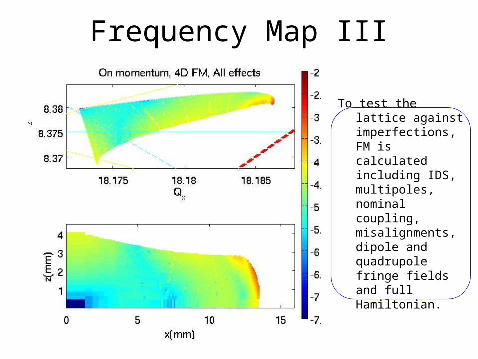
Frequency Map III

To test the lattice against imperfections, FM is calculated including IDS, multipoles, nominal coupling, misalignments, dipole and quadrupole fringe fields and full Hamiltonian.

Non linear dynamics Optimization

Alba layout is fixed, hence we had some time to play around…the sextupole settings (9 families) give margin for optimization.

Traditionally, at Alba, OPA sextupole optimization (analytical hijklp minimization) has been used.

The OPA GUI for sextupole optimization provides a fast and intuitive tool for non linear optimization. However in general, if the optimizer is iterated until convergence, the provided solutions are only good at small amplitudes.

Some effort has been dedicated to find a more systematic (numerical) method for sextupole optimization. AT written in Mathlab and c, provides a good environment for this.

Simplex algorithm has been used with different numerical cost functions. The most successful ones were:

Using AT, The optimization is performed at constant chromaticity (ex: x= y =1). Hence the configuration space has 7 degrees of freedom.

1. DA.2. Tune shifts.3. FFT.

And mostly combinations of these techniques. In all cases, the optimization takes into account off momentum dynamics.

Non linear dynamics Optimization II

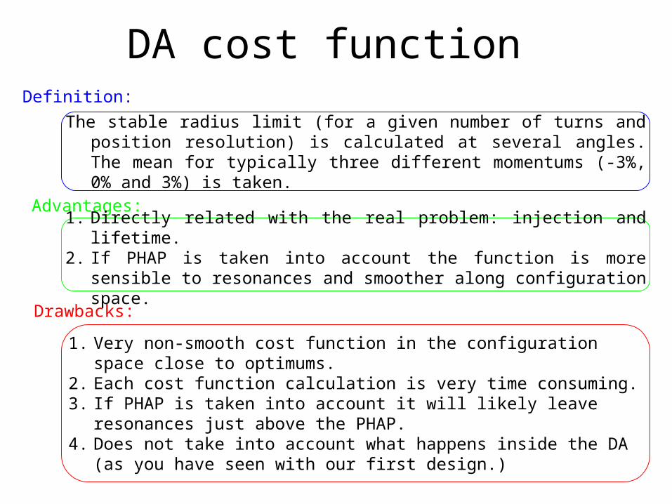
DA cost function

Advantages:

Definition:

Drawbacks:

The stable radius limit (for a given number of turns and position resolution) is calculated at several angles. The mean for typically three different momentums (-3%, 0% and 3%) is taken.

1. Directly related with the real problem: injection and lifetime.2. If PHAP is taken into account the function is more sensible to resonances

and smoother along configuration space.

1. Very non-smooth cost function in the configuration space close to optimums.

2. Each cost function calculation is very time consuming.3. If PHAP is taken into account it will likely leave resonances just above the

PHAP.4. Does not take into account what happens inside the DA (as you have

seen with our first design.)

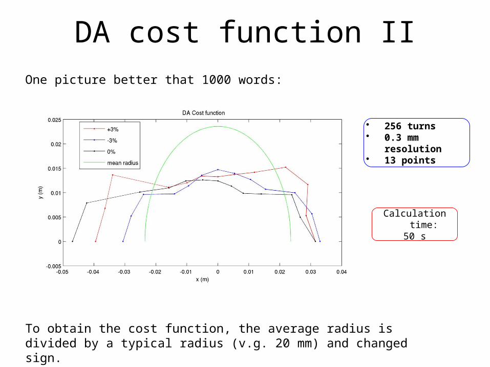
DA cost function IIOne picture better that 1000 words:

To obtain the cost function, the average radius is divided by a typical radius (v.g. 20 mm) and changed sign.

• 256 turns• 0.3 mm resolution• 13 points

Calculation time:50 s

Advantages:

Definition:

Drawbacks:

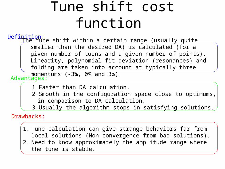
The tune shift within a certain range (usually quite smaller than the desired DA) is calculated (for a given number of turns and a given number of points). Linearity, polynomial fit deviation (resonances) and folding are taken into account at typically three momentums (-3%, 0% and 3%).

1. Faster than DA calculation.2. Smooth in the configuration space close to optimums, in comparison to

DA calculation.3. Usually the algorithm stops in satisfying solutions.

1. Tune calculation can give strange behaviors far from local solutions (Non convergence from bad solutions).

2. Need to know approximately the amplitude range where the tune is stable.

Tune shift cost function

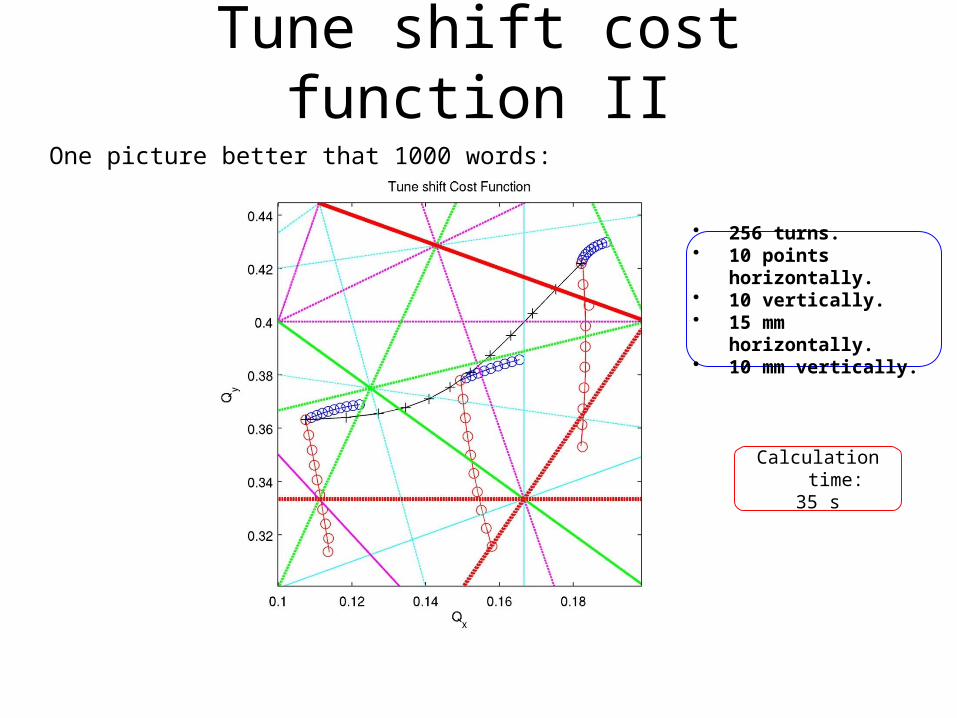
Tune shift cost function IIOne picture better that 1000 words:

• 256 turns.• 10 points horizontally.• 10 vertically.• 15 mm horizontally.• 10 mm vertically.

Calculation time:35 s

Advantages:

Definition:

Drawbacks:

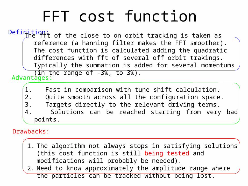
The fft of the close to on orbit tracking is taken as reference (a hanning filter makes the FFT smoother). The cost function is calculated adding the quadratic differences with fft of several off orbit trakings. Typically the summation is added for several momentums (in the range of -3%, to 3%).

1. Fast in comparison with tune shift calculation.2. Quite smooth across all the configuration space.3. Targets directly to the relevant driving terms.4. Solutions can be reached starting from very bad points.

1. The algorithm not always stops in satisfying solutions (this cost function is still being tested and modifications will probably be needed).

2. Need to know approximately the amplitude range where the particles can be tracked without being lost.

FFT cost function

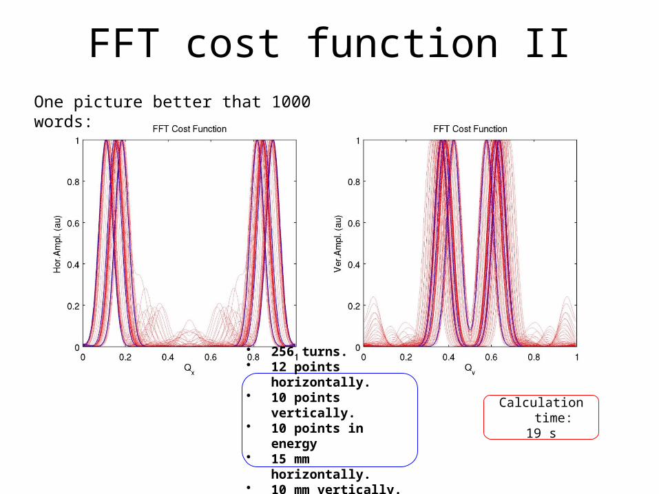
• 256 turns.• 12 points horizontally.• 10 points vertically.• 10 points in energy• 15 mm horizontally.• 10 mm vertically.

One picture better that 1000 words:

FFT cost function II

Calculation time:19 s

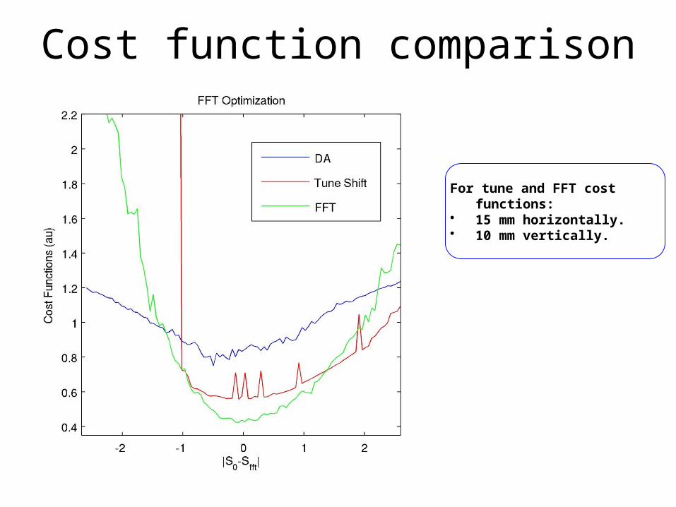
Cost function comparison

For tune and FFT cost functions: • 15 mm horizontally.• 10 mm vertically.

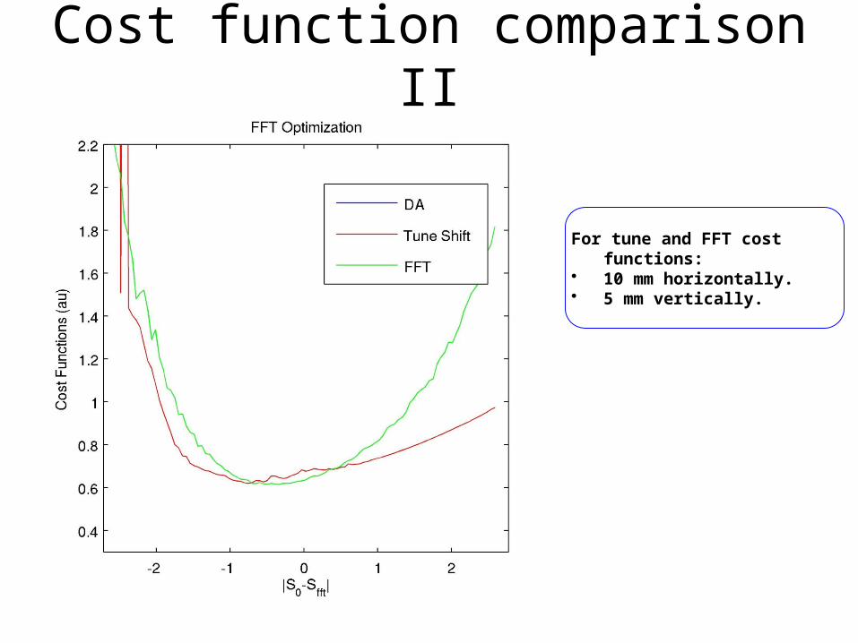
For tune and FFT cost functions: • 10 mm horizontally.• 5 mm vertically.

Cost function comparison II

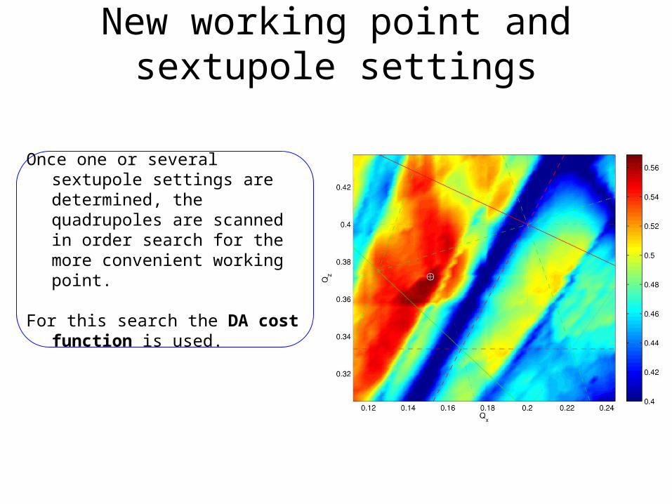
New working point and sextupole settings

Once one or several sextupole settings are determined, the quadrupoles are scanned in order search for the more convenient working point.

For this search the DA cost function is used.

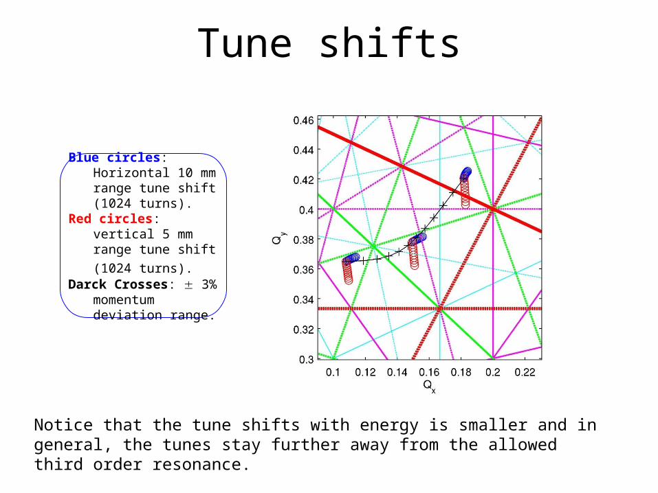
Tune shifts

Blue circles: Horizontal 10 mm range tune shift (1024 turns).

Red circles: vertical 5 mm range tune shift (1024 turns).

Darck Crosses: 3% momentum deviation range.

Notice that the tune shifts with energy is smaller and in general, the tunes stay further away from the allowed third order resonance.

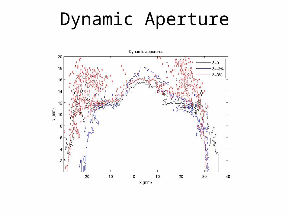
Dynamic Aperture

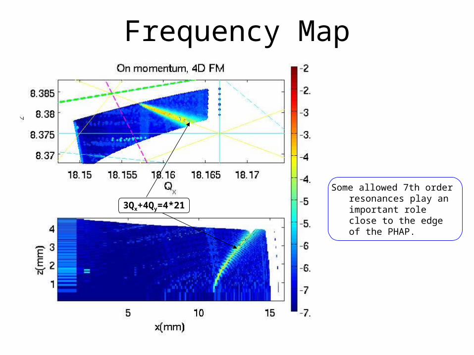
Frequency Map

3Qx+4Qy=4*21Some allowed 7th order

resonances play an important role close to the edge of the PHAP.

Frequency Map II

To test the lattice against imperfections, FM is calculated including IDS, multipoles, nominal coupling, misalignments, dipole and quadrupole fringe fields and full Hamiltonian.

Conclusions1. Alba lattice non linear proprieties have been studied, optimized and tested

against perturbations.2. There is not (or we could not find it) a perfect way to descrive numerically

the non linearities of the lattice. Optimization is done throught several cost functions.

3. Two alternative working points have been presented as fairly good candidates for the operation working point. Final decision could be made based on the future experimental data.

Acknowledgements

This work has been strongly influenced by my bosses during these lat 3 years: M.Muñoz and D.Eindfeld. Also, I owe many thanks to many colleagues, among them G.Benedetti, J.Marcos, P.Campmany, V.Massana…