Nonlinear Regression, Nonlinear Least Squares, and ...change a nonlinear relationship into a linear one (in these data, replacing population by its cube-root linearizes the plot, as

Nonlinear Regression, Nonlinear Least Squares, and Nonlinear

Mixed Models in R

An Appendix to An R Companion to Applied Regression, third edition

John Fox & Sanford Weisberg

last revision: 2018-06-02

Abstract

The nonlinear regression model generalizes the linear regression model by allowing for meanfunctions like E(y|x) = θ1/ {1 + exp[−(θ2 + θ3x)]}, in which the parameters, the θs in this model,enter the mean function nonlinearly. If we assume additive errors, then the parameters in modelslike this one are often estimated via least squares. In this appendix to Fox and Weisberg (2019)we describe how the nls() function in R can be used to obtain estimates, and briefly discusssome of the major issues with nonlinear least squares estimation. We also describe how to usethe nlme() function in the nlme package to fit nonlinear mixed-effects models. Functions inthe car package than can be helpful with nonlinear regression are also illustrated.

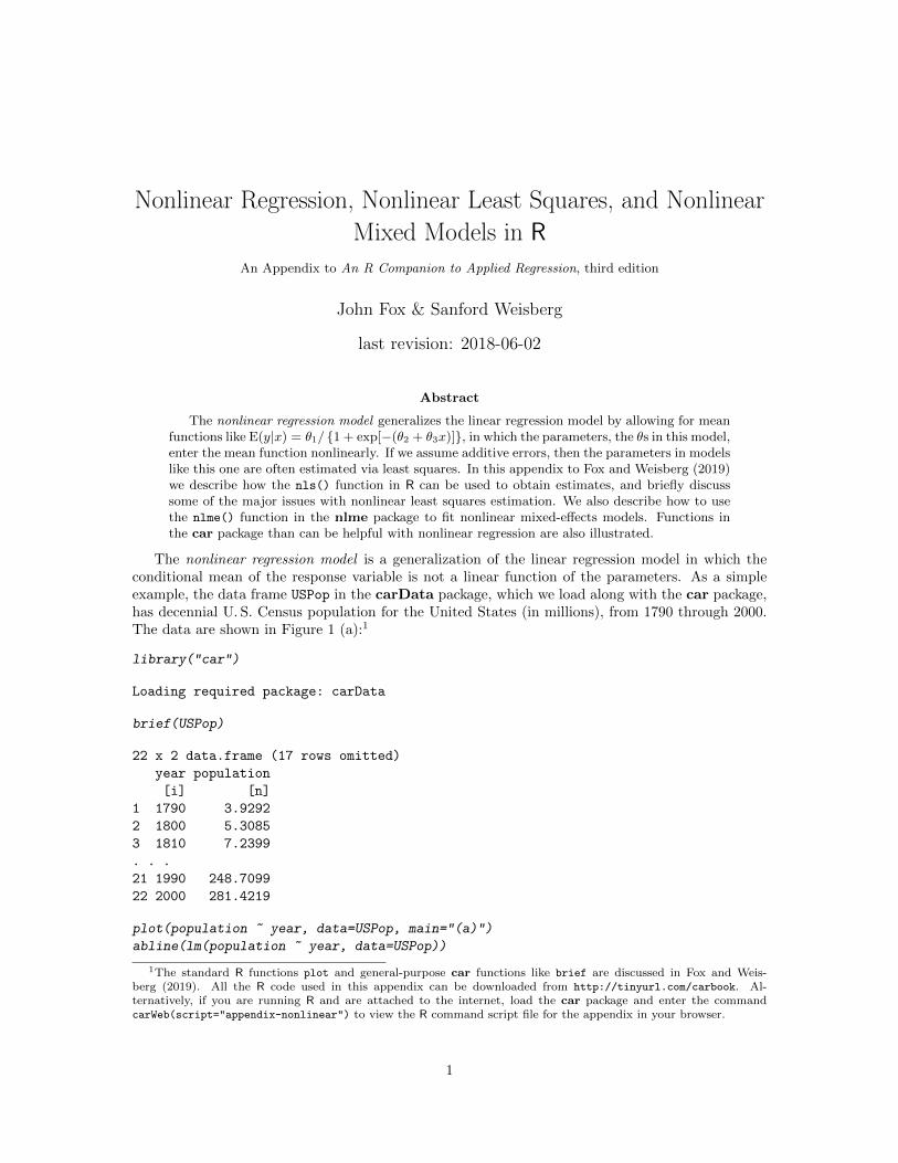
The nonlinear regression model is a generalization of the linear regression model in which theconditional mean of the response variable is not a linear function of the parameters. As a simpleexample, the data frame USPop in the carData package, which we load along with the car package,has decennial U. S. Census population for the United States (in millions), from 1790 through 2000.The data are shown in Figure 1 (a):1

library("car")

Loading required package: carData

brief(USPop)

22 x 2 data.frame (17 rows omitted)

year population

[i] [n]

1 1790 3.9292

2 1800 5.3085

3 1810 7.2399

. . .

21 1990 248.7099

22 2000 281.4219

plot(population ~ year, data=USPop, main="(a)")

abline(lm(population ~ year, data=USPop))

1The standard R functions plot and general-purpose car functions like brief are discussed in Fox and Weis-berg (2019). All the R code used in this appendix can be downloaded from http://tinyurl.com/carbook. Al-ternatively, if you are running R and are attached to the internet, load the car package and enter the commandcarWeb(script="appendix-nonlinear") to view the R command script file for the appendix in your browser.

1

1800 1850 1900 1950 2000

050

100

150

200

250

(a)

year

popu

latio

n

−4 −2 0 2 4

0.0

0.2

0.4

0.6

0.8

1.0

(b)

x

1/(1

+ e

xp(−

(−1

+ 1

* x

)))

Figure 1: (a) U. S. population, from the U. S. Census, and (b) a generic logistic growth curve.

The simple linear regression least-squares line shown on the graph clearly does not match thesedata: The U. S. population is not growing by the same amount in each decade, as is required bythe straight-line model. While in some problems transformation of predictors or the response canchange a nonlinear relationship into a linear one (in these data, replacing population by its cube-rootlinearizes the plot, as can be discovered using the powerTransform() function in the car package),in many instances modeling the nonlinear pattern with a nonlinear mean function is desirable.

A common simple model for population growth is the logistic growth model,

y = m(x,θ) + ε

=θ1

1 + exp[−(θ2 + θ3x)]+ ε (1)

where y is the response, population size in our example, and we will take the predictor x = year.We introduce the notation m(x,θ) for the mean function, which depends on a possibly vector-valuedparameter θ and a possibly vector-valued predictor x, here the single predictor x. More generally,we assume that the predictor vector x consists of fixed, known values.

As a function of x, the mean function in Equation 1 is a curve, as shown in Figure 1 (b) for thespecial case of θ1 = 1, θ2 = 1, θ3 = 1:

curve(1/(1+exp(-(-1 + 1*x))), from=-5, to=5, main="(b)")

abline(h=1/2, v=1, lty=2)

Changing the values of the parameters θ = (θ1, θ2, θ3)′ stretches or shrinks the axes, and changesthe rate at which the curve varies from its lower value at 0 to its maximum value. If θ3 > 0, then asx gets larger the term exp[−(θ2 + θ3x)] gets closer to 0, and so m(x,θ) will approach the value θ1as an asymptote. Assuming logistic population growth therefore imposes a limit to population size.Similarly, again if θ3 > 0, as x → −∞, the term exp[−(θ2 + θ3x)] grows large without bound andso the mean will approach 0. Interpreting the meaning of θ2 and θ3 is more difficult. The logisticgrowth curve is symmetric about the value of x for which m(x,θ) is midway between 0 and θ1. It isnot hard to show that m(x = −θ2/θ3,θ) = θ1/2, and so the curve is symmetric about the midpointx = −θ2/θ3. The parameter θ3 controls how quickly the curve transitions from the lower asymptoteof 0 to the upper asymptote at θ1, and is therefore a growth-rate parameter.

2

It is not obvious that a curve of the shape in Figure 1 (b) can match the data shown in Figure 1(a), but a part of the curve, from about x = −3 to x = 2, may be able to fit the data fairlywell. Fitting the curve corresponds to estimating parameters to get a logistic growth function thatmatches the data. Determining whether extrapolation of the curve outside this range makes senseis beyond the scope of this brief report.

1 Fitting Nonlinear Regressions with the nls() Function

The standard nls() function in R is used for estimating parameters via nonlinear least squares.Following Weisberg (2014, Chap. 11), the general nonlinear regression model is2

y = E(y|x) + ε = m(x,θ) + ε

This model posits that the mean E(y|x) depends on x through the kernel mean function m(x,θ),where the predictor x has one or more components and the parameter vector θ also has one or morecomponents. In the logistic growth example in Equation 1, x consists of the single predictor x = year

and the parameter vector θ = (θ1, θ2, θ3)′ has three components. The model further assumes thatthe errors ε are independent with variance σ2/w, where the w are known nonnegative weights, andσ2 is a generally unknown variance to be estimated from the data.3 In many applications w = 1 forall observations.

The nls() function can be used to estimate θ as the values that minimize the residual sum ofsquares,

S(θ) =∑

w [y −m(θ,x)]2

(2)

We will write θ̂ for the minimizer of the residual sum of squares.Unlike the linear least-squares problem, there is usually no closed-form formula that provides the

minimizer of Equation 2. An iterative procedure is used, which in broad outline is as follows:

1. The user supplies an initial guess, say t0 of starting values for the parameters. Whether or notthe algorithm can successfully find a minimizer will depend on getting starting values that arereasonably close to the solution. We discuss how this might be done for the logistic growthfunction below. For some special mean functions, including logistic growth, R has self-startingfunctions that can avoid this step.

2. At iteration j ≥ 1, the current guess tj is obtained by updating tj−1. If S(tj) is smaller thanS(tt−1) by at least a predetermined amount, then the counter j is increased by 1 and this step

is repeated. If no such improvement is possible, then tj−1 is taken as the estimator θ̂ of θ.

This simple algorithm hides at least three important considerations. First, we want a method thatwill guarantee that at each step we either get a smaller value of S or at least S will not increase. Thereare many nonlinear least-squares algorithms; see, for example, Bates and Watts (1988). Many algo-rithms make use of the derivatives of the mean function with respect to the parameters. The defaultalgorithm in nls() uses a form of Gauss-Newton iteration that employs derivatives approximatednumerically unless we provide functions to compute the derivatives. Second, the sum-of-squaresfunction S may be a perverse function with multiple minima. As a consequence, the purportedleast-squares estimates could be a local rather than global minimizer of S. Third, as given thealgorithm can go on forever if improvements to S are small at each step. As a practical matter,therefore, there is an iteration limit that specifies the maximum number of iterations permitted, anda tolerance that defines the minimum improvement that will be considered to be greater than 0.

The call to nls() is similar to the call to lm() for linear models. Here are the arguments:

2Also see Fox (2016, Sec. 17.4)3The assumption of independent errors is often untenable for time-series data such as the U. S. population data,

where errors may be substantially autocorrelated. See the appendix on time-series regression.

3

args(nls)

function (formula, data = parent.frame(), start, control = nls.control(),

algorithm = c("default", "plinear", "port"), trace = FALSE,

subset, weights, na.action, model = FALSE, lower = -Inf,

upper = Inf, ...)

NULL

We discuss each of these arguments in turn:

formula The formula argument is used to tell nls() about the mean function. The formula equiv-alent to Equation 1 (page 2) is

population ~ theta1/(1 + exp(-(theta2 + theta3*year)))

As in lm(), the left side of the formula specifies the response variable, and is followed by thetilde (˜) as a separator that is commonly read as “is regressed on” or “is modeled by.” The rightside of the formula for nonlinear models is very different from lm() models. In the simplest formfor nls(), the right side is a mathematical expression consisting of constants, like the number1; predictors, in this case just year; named parameters like theta1, theta2 and theta3; andmathematical functions and operators like exp() for exponentiation, / for division and + foraddition. Factors, interactions, and in general the Wilkinson-Rogers notation employed forlinear models, are not used with nls(). Parentheses are used with the usual precedence rulesfor mathematics, but square brackets “[ ]” and curly braces “{ }” cannot be used. If values ofthe parameters and predictors were specified, then the right side of the formula would evaluateto a number. We can name the parameters with any legal R names, such as theta1, alpha,t1, or Asymptote.

The formula for nls() can take several other forms beyond the sample form described here.We will use a few other forms in later sections of this appendix, but even so we won’t describethis argument in full generality.

start The argument start is a list that tells nls() which of the named quantities on the right sideof the formula are parameters, and thus implicitly which are predictors. The argument also pro-vides starting values for the parameter estimates. For the example, start=list(theta1=440,theta2= -4, theta3=0.2) names the thetas as the parameters and also specifies startingvalues for them. Since year has no starting value, it is taken by nls() to be a predictor. Thestart argument is required unless a self-starting function is used in the formula argument.

algorithm = "default" The "default" algorithm used in nls() is a Gauss-Newton algorithm.Other possible values are "plinear" for the Golub-Pereyra algorithm for partially linear modelsand "port" for a algorithm that should be selected if there are constraints on the parameters(see the next argument). The help page for nls() gives references.

lower = -Inf, upper = Inf Parameters of the model might be constrained to lie in a certain region.In the logistic population-growth model, for example, we must have θ3 > 0, as population sizeis increasing, and we must also have θ1 > 0. In some problems we would like to be certainthat the algorithm never considers values for θ outside the feasible range. The argumentslower and upper are vectors of lower and upper bounds, replicated to be as long as start.If unspecified, all parameters are assumed to be unconstrained. Bounds can only be used withthe "port" algorithm. They are ignored, with a warning, if given for other algorithms.

control = nls.control() This argument is set to a call to the nls.control() function, whichmay be used to modify characteristics of the computing algorithm:

4

args(nls.control)

function (maxiter = 50, tol = 1e-05, minFactor = 1/1024, printEval = FALSE,

warnOnly = FALSE)

NULL

Users will generally be concerned with the control argument only if convergence problemsare encountered. For example, to change the maximum number of iterations to 40 and theconvergence tolerance to 10−6, set control=nls.control(maxiter=40, tol=1e-6).

trace = FALSE If TRUE, print the value of the residual sum of squares and the parameter estimatesat each iteration. The default is FALSE.

data, subset, na.action, weights These arguments are the same as for lm(), with data, subset,and na.action specifying the data to which the model is to be fit, and weights giving theweights w to be used for the least-squares fit. If the weights argument is missing then allweights are set equal to 1.

2 Starting Values

Most nonlinear least-squares algorithms require specification of starting values for the parameters,which are θ1, θ2 and θ3 for the logistic growth model of Equation 1 (page 2).4 There are many waysto determine starting values in nonlinear regression, but they generally require consideration of themathematical form of the model. For the logistic growth model, for example, we can write

y ≈ θ11 + exp[−(θ2 + θ3x)]

y/θ1 ≈ 1

1 + exp[−(θ2 + θ3x)]

log

[y/θ1

1− y/θ1

]≈ θ2 + θ3x

The first of these three equations is the original logistic growth function. In the second equation,we divide through by the asymptote θ1, so the left side is now a positive number between 0 and 1.We then apply the logit transformation, as in binomial regression with a logit link, to get a linearmodel. Consequently, if we have a starting value t1 for θ1 we can compute starting values for theother θs by the OLS linear regression of the logit of y/t1 on x.

A starting value of the asymptote θ1 should be some value larger than any value in the data,and so a value of around t1 = 400 is a reasonable choice. (The Census count for 2010, which wedeliberately omitted from the data, was 308,745,538.) Using lm() and the logit() function fromthe car package, we compute starting values for the other two parameters:

lm(logit(population/400) ~ year, USPop)

Call:

lm(formula = logit(population/400) ~ year, data = USPop)

Coefficients:

(Intercept) year

-49.2499 0.0251

4Generalized linear models use a similar iterative estimation method, but finding starting values is usually notimportant because a set of default starting values is almost always adequate.

5

Thus, starting values for the other θs are t2 = −49 and t3 = 0.025.

pop.mod <- nls(population ~ theta1/(1 + exp(-(theta2 + theta3*year))),

start=list(theta1 = 400, theta2 = -49, theta3 = 0.025),

data=USPop, trace=TRUE)

3060.8 : 400.000 -49.000 0.025

558.54 : 426.061991 -42.307856 0.021421

457.97 : 438.414699 -42.836902 0.021677

457.81 : 440.890336 -42.698662 0.021602

457.81 : 440.816807 -42.708050 0.021606

457.81 : 440.834471 -42.706883 0.021606

457.81 : 440.833344 -42.706977 0.021606

By setting trace=TRUE, we can see that S evaluated at the starting values is 3061. The first iterationreduces this to 558.5, the next iteration to 458, and the remaining iterations result in only very smallchanges. We get convergence in 6 iterations.

We use the summary() function to print a report for the fitted model:

summary(pop.mod)

Formula: population ~ theta1/(1 + exp(-(theta2 + theta3 * year)))

Parameters:

Estimate Std. Error t value Pr(>|t|)

theta1 440.83334 35.00014 12.6 1.1e-10

theta2 -42.70698 1.83914 -23.2 2.1e-15

theta3 0.02161 0.00101 21.4 8.9e-15

Residual standard error: 4.91 on 19 degrees of freedom

Number of iterations to convergence: 6

Achieved convergence tolerance: 1.24e-06

The column marked Estimate displays the least squares estimates of the parameters. The estimatedupper bound for the U. S. population is thus 440.8, or about 441 million. The column markedStd. Error displays the standard errors of thes estimated regression coefficients. The very largestandard error for the θ̂1 reflects the uncertainty in the estimated asymptote when all the observeddata are much smaller than the asymptote. The estimated year in which the population is halfthe asymptote is −θ̂3/θ̂2 = 1976.6. The standard error of this estimate can be computed by thedeltaMethod() function in the car package:

deltaMethod(pop.mod, "-theta2/theta3")

Estimate SE 2.5 % 97.5 %

-theta2/theta3 1976.6 7.5558 1961.8 1991.4

and so the standard error is about 7.6 years.The column t value in the summary() output shows the ratio of each parameter estimate to its

standard error. In sufficiently large samples, this ratio will generally have a normal distribution, butinterpreting “sufficiently large” is difficult with nonlinear models. Even if the errors ε are normallydistributed, the estimates may be far from normally distributed in small samples. The p-values shown

6

are based on asymptotic normality, and test the null hypotheses that each θ is equal to 0. In thisexample, and frequently in nonlinear models, these hypotheses are not really of interest; for example,it isn’t sensible to suppose that the asymptotic population of the U. S. is 0. The residual standarddeviation is the estimate of σ,

σ̂ =

√S(θ̂)/(n− k)

where k is the number of parameters in the mean function, 3 in this example.The Confint() function in the car package can be used to get confidence intervals for each of

the parameter estimates. These intervals are based on the profile log-likelihood, and are generallymuch more accurate than are intervals based on asymptotic normality:

Confint(pop.mod)

Waiting for profiling to be done...

Estimate 2.5% 97.5%

theta1 440.833344 381.493655 536.938593

theta2 -42.706977 -46.586310 -39.110835

theta3 0.021606 0.019613 0.023719

Many familiar generic functions, such as residuals(), have methods for the nonlinear-modelobjects produced by nls(). For example, the predict() function makes it simple to plot the fit ofthe model as in Figure 2:

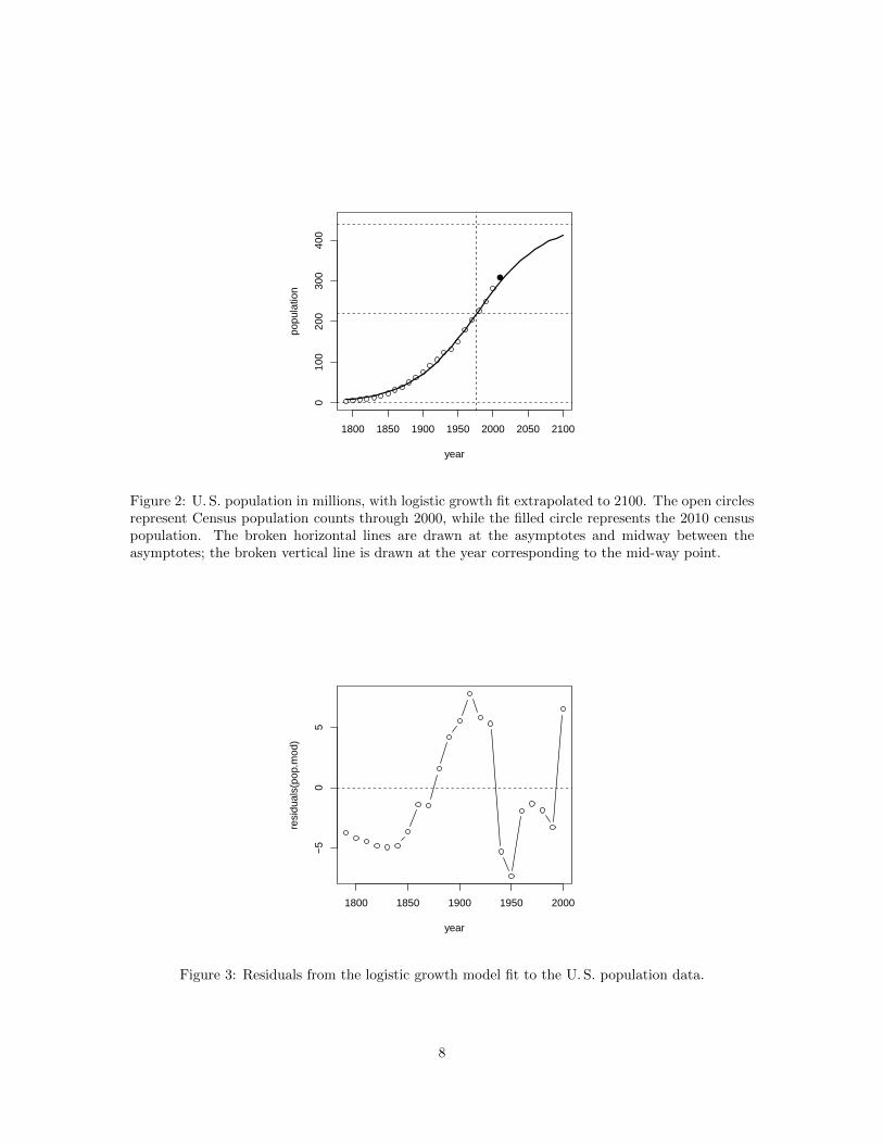
plot(population ~ year, USPop, xlim=c(1790, 2100), ylim=c(0, 450))

with(USPop, lines(seq(1790, 2100, by=10),

predict(pop.mod, data.frame(year=seq(1790, 2100, by=10))), lwd=2))

points(2010, 308.745538, pch=16, cex=1.3)

abline(h=0, lty=2)

abline(h=coef(pop.mod)[1], lty=2)

abline(h=0.5*coef(pop.mod)[1], lty=2)

abline(v= -coef(pop.mod)[2]/coef(pop.mod)[3], lty=2)

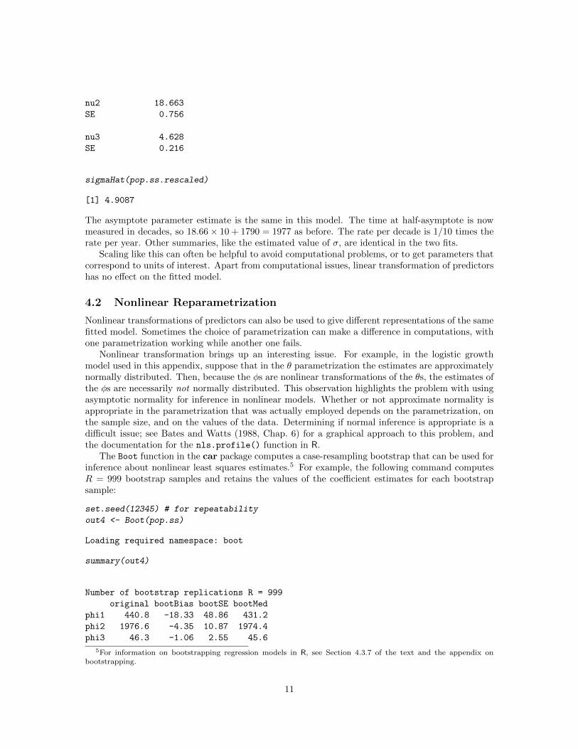
We made this plot more complicated than necessary simply to display the fit of the logistic modelto the data, in order to show the shape of the fitted curve projected into the future, to include theCensus population in 2010, and to add lines for the asymptotes and for the point half way betweenthe asymptotes. While Figure 2 confirms that the logistic growth mean function generally matchesthe data, the residual plot in Figure 3 suggests that there are systematic features that are missed,reflecting differences in growth rates, perhaps due to factors such as changes in immigration policies:

with(USPop, plot(year, residuals(pop.mod), type='b'))

abline(h=0, lty=2)

3 Self-Starting Models

Bates and Watts (1988, Sec. 3.2) describe many techniques for finding starting values for fittingnonlinear models. For the logistic growth model described in this paper, for example, finding startingvalues amounts to (1) guessing the parameter θ1 as a value larger than any observed in the data; and(2) substituting this value into the mean function, rearranging terms, and then getting other startingvalues by OLS simple linear regression. This algorithm can of course be written as an R function toget starting values automatically, and this is the basis of the self-starting nonlinear models describedby Pinheiro and Bates (2000, Sec. 8.1.2).

7

1800 1850 1900 1950 2000 2050 2100

010

020

030

040

0

year

popu

latio

n

Figure 2: U. S. population in millions, with logistic growth fit extrapolated to 2100. The open circlesrepresent Census population counts through 2000, while the filled circle represents the 2010 censuspopulation. The broken horizontal lines are drawn at the asymptotes and midway between theasymptotes; the broken vertical line is drawn at the year corresponding to the mid-way point.

1800 1850 1900 1950 2000

−5

05

year

resi

dual

s(po

p.m

od)

Figure 3: Residuals from the logistic growth model fit to the U. S. population data.

8

The self-starting logistic growth model in R is based on a different, but equivalent, parametriza-tion of the logistic function. We will start again with the logistic growth model, with mean function

m(x,θ) =θ1

1 + exp[−(θ2 + θ3x)]

We have seen that the ratio −θ2/θ3 is an interesting function of the θs, and so we might reparametrizethis mean function as:

m(x,φ) =φ1

1 + exp[−(x− φ2)/φ3]

As the reader can verify, we have defined φ1 = θ1 φ2 = −θ2/θ3, and φ3 = 1/θ3. In the φ-parametrization, φ1 is the upper asymptote, φ2 is the value of x at which the response is half itsasymptotic value, and φ3 is a rate parameter. Because the φ-parameters are a one-to-one nonlineartransformation of the θ-parameters, the two models provide the same fit to the data.

Fitting a nonlinear model with the self-starting logistic growth function in R is quite easy:

pop.ss <- nls(population ~ SSlogis(year, phi1, phi2, phi3), data=USPop)

summary(pop.ss)

Formula: population ~ SSlogis(year, phi1, phi2, phi3)

Parameters:


phi1 440.83 35.00 12.6 1.1e-10

phi2 1976.63 7.56 261.6 < 2e-16

phi3 46.28 2.16 21.4 8.9e-15

Residual standard error: 4.91 on 19 degrees of freedom



The right side of the formula is now the name of a function that has the responsibility for computingthe mean function and for finding starting values. The estimate of the asymptote parameter φ1 andits standard error are identical to the estimate and standard error for θ̂1 in the θ-parametrization.Similarly, the estimate for φ2 and its standard error are identical to the estimate and standard errorfor −θ2/θ3 obtained from the delta method (page 6). Finally, applying the delta method again,

deltaMethod(pop.mod, "1/theta3")


1/theta3 46.284 2.1574 42.055 50.512

we see that φ̂3 = 1/θ̂3 with the same standard error from the delta method as from the φ-parametrized model.

Table 1 lists the self-starting nonlinear functions that are available in the standard R system.Pinheiro and Bates (2000, Sec. 8.1.2) discuss how users can make their own self-starting functions.

4 Parametrization

4.1 Linear Reparametrization

In some problems it may be useful to transform a predictor linearly to make the resulting parametersmore meaningful. In the U. S. population data, we might consider replacing the predictor year bydecade = (year− 1790)/10.

9

Function Equation, m(x, φ) =SSasymp Asymptotic regression

φ1 + (φ2 − φ1) exp[− exp(φ3)x]SSasympOff() Asymptotic regression with an offset

φ1{1− exp[− exp(φ2)× (x− φ3)]}SSasympOrig() Asymptotic regression through the origin

φ1{1− exp[− exp(φ2)x]}SSbiexp() Biexponential model

φ1 exp[− exp(φ2)x] + φ3 exp[− exp(φ4)x]SSfol() First-order compartment model

D exp(φ1+φ2)exp(φ3)[exp(φ2)−exp(φ1)]

{exp[− exp(φ1)x]− exp([− exp(φ2)x]}SSfpl() Four-parameter logistic growth model

φ1 + φ2−φ2

1+exp[(φ3−x)/φ4]

SSgompertz() Gompertz modelφ1 exp(φ2x

φ3)SSlogis() Logistic model

φ1/(1 + exp[(φ2 − x)/φ3])SSmicmen() Michaelis-Menten model

φ1x/(φ2 + x)SSweibull() Weibull model

φ1 + (φ2 − φ1) exp[− exp(φ3)xφ4 ]

Table 1: The self-starting functions available in R, from Pinheiro and Bates (2000, Appendix C).Tools are also available for users to write their own self-starting functions.

USPop$decade <- (USPop$year - 1790)/10

pop.ss.rescaled <- nls(population ~ SSlogis(decade, nu1, nu2, nu3), data=USPop)

compareCoefs(pop.ss, pop.ss.rescaled)

Calls:

1: nls(formula = population ~ SSlogis(year, phi1, phi2, phi3),

data = USPop, algorithm = "default", control = list(maxiter =

50, tol = 1e-05, minFactor = 0.0009765625, printEval = FALSE,

warnOnly = FALSE), trace = FALSE)

2: nls(formula = population ~ SSlogis(decade, nu1, nu2, nu3),

data = USPop, algorithm = "default", control = list(maxiter =

50, tol = 1e-05, minFactor = 0.0009765625, printEval = FALSE,

warnOnly = FALSE), trace = FALSE)

Model 1 Model 2

phi1 441

SE 35

phi2 1976.63

SE 7.56

phi3 46.28

SE 2.16

nu1 441

SE 35

10

nu2 18.663

SE 0.756

nu3 4.628

SE 0.216

sigmaHat(pop.ss.rescaled)

[1] 4.9087

The asymptote parameter estimate is the same in this model. The time at half-asymptote is nowmeasured in decades, so 18.66× 10 + 1790 = 1977 as before. The rate per decade is 1/10 times therate per year. Other summaries, like the estimated value of σ, are identical in the two fits.

Scaling like this can often be helpful to avoid computational problems, or to get parameters thatcorrespond to units of interest. Apart from computational issues, linear transformation of predictorshas no effect on the fitted model.

4.2 Nonlinear Reparametrization

Nonlinear transformations of predictors can also be used to give different representations of the samefitted model. Sometimes the choice of parametrization can make a difference in computations, withone parametrization working while another one fails.

Nonlinear transformation brings up an interesting issue. For example, in the logistic growthmodel used in this appendix, suppose that in the θ parametrization the estimates are approximatelynormally distributed. Then, because the φs are nonlinear transformations of the θs, the estimates ofthe φs are necessarily not normally distributed. This observation highlights the problem with usingasymptotic normality for inference in nonlinear models. Whether or not approximate normality isappropriate in the parametrization that was actually employed depends on the parametrization, onthe sample size, and on the values of the data. Determining if normal inference is appropriate is adifficult issue; see Bates and Watts (1988, Chap. 6) for a graphical approach to this problem, andthe documentation for the nls.profile() function in R.

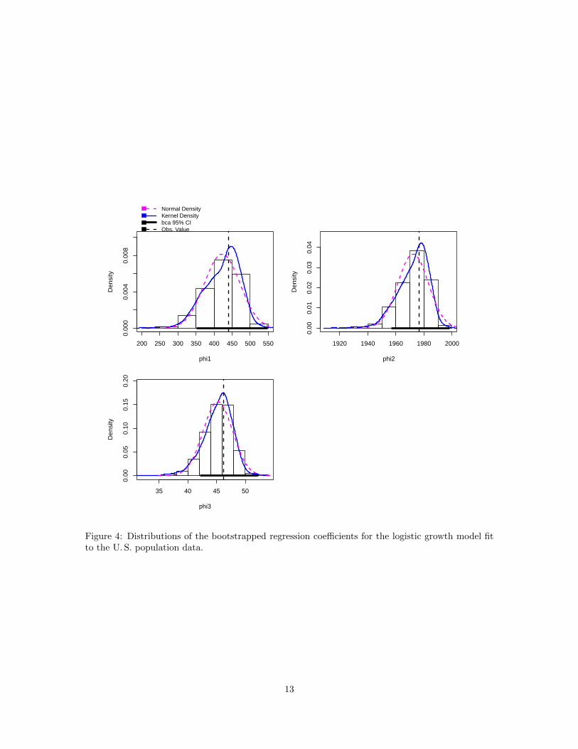
The Boot function in the car package computes a case-resampling bootstrap that can be used forinference about nonlinear least squares estimates.5 For example, the following command computesR = 999 bootstrap samples and retains the values of the coefficient estimates for each bootstrapsample:

set.seed(12345) # for repeatability

out4 <- Boot(pop.ss)

Loading required namespace: boot

summary(out4)

Number of bootstrap replications R = 999

original bootBias bootSE bootMed

phi1 440.8 -18.33 48.86 431.2

phi2 1976.6 -4.35 10.87 1974.4

phi3 46.3 -1.06 2.55 45.6

5For information on bootstrapping regression models in R, see Section 4.3.7 of the text and the appendix onbootstrapping.

11

hist(out4)

Confint(out4)

Bootstrap bca confidence intervals

Estimate 2.5 % 97.5 %

phi1 440.833 353.380 545.613

phi2 1976.634 1957.428 1997.657

phi3 46.284 42.208 52.215

The differences between the original estimates and the bootstrap means, recorded in the columnnamed bootBias, suggest substantial bias in the estimates. The nominal standard errors reportedin summary output for the model on page 9 are also considerably smaller than the standard errorsbased on the bootstrap. Histograms and density estimates of the bootstrap samples, produced bythe hist() function and shown in Figure 4, reveal that the marginal distribution of each parameterestimate is moderately to severely skewed, suggesting that inference based on asymptotic normality isa poor idea. By default, the Confint() function reports BCa biased-corrected bootstrap confidenceintervals, which also appear in the graphs produced by hist(): See ?Confint.boot and ?hist.boot.

5 Nonlinear Mean Functions

Some problems will dictate the form of the nonlinear mean function that is of interest, possiblythrough theoretical considerations, differential equations, and the like. In other cases, the choiceof a mean function is largely arbitrary, as only qualitative characteristics of the curve, such as theexistence of an asymptote, are known in advance. Ratkowsky (1990) provides a very helpful catalogof nonlinear mean functions that are commonly used in practice, a catalog that both points out thevariety of available functions and some of the ambiguity in selecting a particular function to study.

For example, consider the following three-parameter asymptotic regression models:

m1(x,θ) = α− βγx

m2(x,θ) = α− β exp(−κx)

m3(x,θ) = α{1− exp[−κ(x− ζ)]}m4(x,θ) = α+ (µ− α)γx

m5(x,θ) = α+ (µ− α) exp(−κx)

m6(x,θ) = α− exp[−(δ + κx)]

m7(x,θ) = θ1 + β[1− exp(−κx)]

All of these equations describe exactly the same function! In each equation, α corresponds to theasymptote as x→∞, β = α− µ is the range of y from its minimum to its maximum, µ is the meanvalue of y when x = 0, δ = log(β) is the log of the range, ζ is the value of x when the mean responseis 0, and κ and γ are rate parameters. Many of these functions have names in particular areas ofstudy; for example, m3(x,θ) is called the von Bertalanffy function and is commonly used in thefisheries literature to model fish growth. Ratkowsky (1990, Sec. 4.3) points out that none of theseparametrizations dominates the others with regard to computational and asymptotic properties.Indeed, other parametrizations of this same function may be used in some circumstances. Forexample, Weisberg et al. (2010) reparametrize m3(x,θ) as

m30(x,θ) = α{1− exp[−(log(2)/κ0)(x− ζ)]}

If x is the age of an organism, then in this parametrization the transformed rate parameter κ0 is theage at which the size y of the organism is expected to be one-half its asymptotic size.

12

phi1

Den

sity

200 250 300 350 400 450 500 550

0.00

00.

004

0.00

8

Normal DensityKernel Densitybca 95% CIObs. Value

phi2

Den

sity

1920 1940 1960 1980 2000

0.00

0.01

0.02

0.03

0.04

phi3

Den

sity

35 40 45 50

0.00

0.05

0.10

0.15

0.20

Figure 4: Distributions of the bootstrapped regression coefficients for the logistic growth model fitto the U. S. population data.

13

6 Nonlinear Models Fit with a Factor

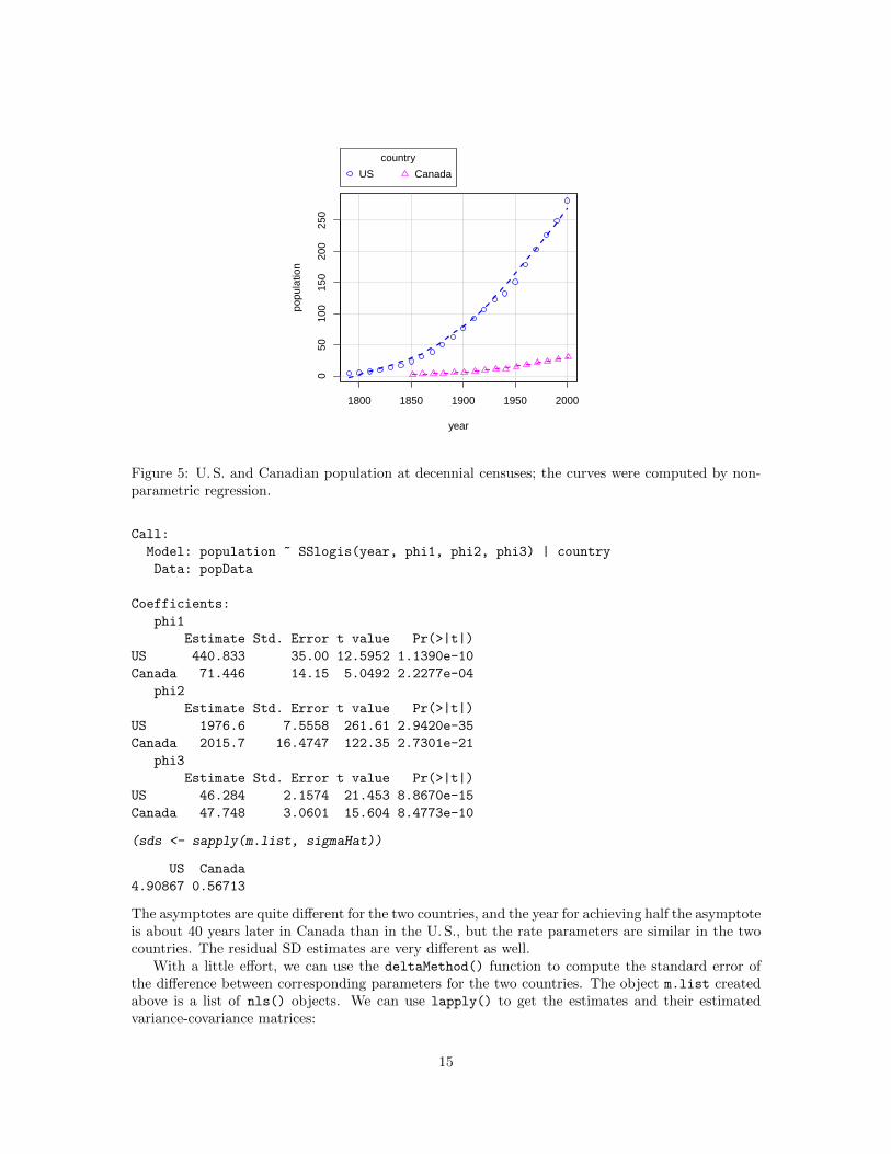
A common problem with nonlinear models is fitting the same mean function to each of several groupsof data. For example, the data frame CanPop in the car package has Canadian population data inthe same format at the U. S. data. We combine the two data frames into one, and then draw a graphof the data for both countries:

brief(CanPop)


year population

[n] [n]

1 1851 2.436

2 1861 3.230

3 1871 3.689

. . .

15 1991 26.429

16 2001 30.007

popData <- data.frame(rbind(data.frame(country="US", USPop[,1:2]),

data.frame(country="Canada", CanPop)))

brief(popData)


country year population

[f] [n] [n]

1 US 1790 3.9292

2 US 1800 5.3085

3 US 1810 7.2399

. . .

151 Canada 1991 26.4290

161 Canada 2001 30.0070

The combined data frame has a new variable called country with values US or Canada. The brief()function from the car package displays a few of the rows of popData.

scatterplot(population ~ year|country, data=popData, box=FALSE,

reg=FALSE)

The scatterplot() function in the car package allows for automatic differentiation of the points bygroups. Setting both box and reg to FALSE suppresses the irrelevant boxplots and simple-regressionlines, respectively. The lines shown on the plot are nonparametric smooths, which we could alsohave suppressed by adding smooth=FALSE to the function call.

We can fit a logistic growth mean function separately to each country. The nlsList() functionin the nlme package (Pinheiro and Bates, 2000) makes this easy. By default nlsList() assumesthe same variance for the errors in all groups, but this is not appropriate in this example becausethe population counts for the larger U. S. are more variable than the counts for Canada. We use theargument pool=FALSE to force separate estimates of error variance for the two countries:

library("nlme")

m.list <- nlsList(population ~ SSlogis(year, phi1, phi2, phi3)|country,

pool=FALSE, data=popData)

summary(m.list)

14

1800 1850 1900 1950 2000

050

100

150

200

250

year

popu

latio

n

country

US Canada

Figure 5: U. S. and Canadian population at decennial censuses; the curves were computed by non-parametric regression.

Call:

Model: population ~ SSlogis(year, phi1, phi2, phi3) | country

Data: popData

Coefficients:

phi1


US 440.833 35.00 12.5952 1.1390e-10

Canada 71.446 14.15 5.0492 2.2277e-04

phi2


US 1976.6 7.5558 261.61 2.9420e-35

Canada 2015.7 16.4747 122.35 2.7301e-21

phi3


US 46.284 2.1574 21.453 8.8670e-15

Canada 47.748 3.0601 15.604 8.4773e-10

(sds <- sapply(m.list, sigmaHat))

US Canada

4.90867 0.56713

The asymptotes are quite different for the two countries, and the year for achieving half the asymptoteis about 40 years later in Canada than in the U. S., but the rate parameters are similar in the twocountries. The residual SD estimates are very different as well.

With a little effort, we can use the deltaMethod() function to compute the standard error ofthe difference between corresponding parameters for the two countries. The object m.list createdabove is a list of nls() objects. We can use lapply() to get the estimates and their estimatedvariance-covariance matrices:

15

(betas <- lapply(m.list, coef))

$US

phi1 phi2 phi3

440.833 1976.634 46.284

$Canada

phi1 phi2 phi3

71.446 2015.663 47.748

(vars <- lapply(m.list, vcov))

$US

phi1 phi2 phi3

phi1 1225.012 262.854 69.1283

phi2 262.854 57.090 15.2287

phi3 69.128 15.229 4.6546

$Canada

phi1 phi2 phi3

phi1 200.225 232.479 40.835

phi2 232.479 271.416 48.461

phi3 40.835 48.461 9.364

We then use unlist to combine the estimates into a single vector, and also combine the two covari-ance matrices into a single block-diagonal matrix; the block-diagonal structure makes sense becausewe have independent estimates of the parameters for the two countries:

(betas <- unlist(betas))

US.phi1 US.phi2 US.phi3 Canada.phi1 Canada.phi2

440.833 1976.634 46.284 71.446 2015.663

Canada.phi3

47.748

zero <- matrix(0, nrow=3, ncol=3)

(var <- rbind( cbind(vars[[1]], zero), cbind(zero, vars[[2]])))

phi1 phi2 phi3

phi1 1225.012 262.854 69.1283 0.000 0.000 0.000

phi2 262.854 57.090 15.2287 0.000 0.000 0.000

phi3 69.128 15.229 4.6546 0.000 0.000 0.000

phi1 0.000 0.000 0.0000 200.225 232.479 40.835

phi2 0.000 0.000 0.0000 232.479 271.416 48.461

phi3 0.000 0.000 0.0000 40.835 48.461 9.364

deltaMethod(betas, "US.phi3 - Canada.phi3", vcov=var)


US.phi3 - Canada.phi3 -1.4645 3.7441 -8.8028 5.8739

deltaMethod(betas, "US.phi2 - Canada.phi2", vcov=var)


US.phi2 - Canada.phi2 -39.029 18.125 -74.553 -3.5051

16

The rate parameters differ by about half a standard error of the difference, while the times athalf-asymptotic population differ by about two standard errors, with the U. S. earlier.

If we number the countries as k = 1, 2 for the U. S. and Canada respectively, then the model fitby nlsList() is

yk(x) =φ1k

1 + exp[−(x− φ2k)/φ3k]+ εk

Interesting hypotheses could consist of testing φ21 = φ22, φ31 = φ32, or both of these. We nowproceed to test these relevant hypotheses in R using likelihood-ratio tests. Because the error variancesare different for the two countries, we can do this only approximately, by setting weights as follows:

w <- ifelse(popData$country == "Canada", (sds[1]/sds[2])^2, 1)

head(w) # first few for U.S.

[1] 1 1 1 1 1 1

tail(w) # last few for Canada

[1] 74.914 74.914 74.914 74.914 74.914 74.914

This procedure adjusts the residual sum of squares for the combined data to give the same standarderrors we obtained using nlsList(). To get exact tests we would need to weight according to theunknown population variance ratio, rather than the sample variance ratio.

We let can be a dummy variable that has the value 1 for Canada and 0 for the U. S.,

popData$can <- ifelse(popData$country == "Canada", 1, 0)

The largest model we contemplate has separate parameters for each country. We fit this model firstdefining the formula, then getting starting values from m.list, and finally computing the fit:

form1 <- population ~ (1 - can)*(phi11/(1 + exp(-(year - phi21)/phi31))) +

can*(phi12/(1 + exp(-(year - phi22)/phi32)))

b <- coef(m.list)

m1 <- nls(form1, data=popData, weights=w,

start=list(phi11=b[1, 1], phi12=b[1, 2], # U.S.

phi21=b[1, 2], phi22=b[2, 2], phi31=b[1, 3], phi32=b[2, 3])) # Canada

A model with the same rate parameter for the two countries, φ31 = φ32 = φ3, is

form2 <- population ~ (1 - can)*(phi11/(1 + exp(-(year - phi21)/phi3))) +

can*(phi12/(1 + exp(-(year - phi22)/phi3)))

m2 <- nls(form2, data=popData, weights=w, start=list(phi11=b[1, 1], phi12=b[1, 2],

phi21=b[1, 2], phi22=b[2, 2], phi3=b[1, 3]))

The anova function can be used to get the (approximate, because of weighting) likelihood-ratio testof equal rate parameters:

anova(m2, m1)

Analysis of Variance Table

Model 1: population ~ (1 - can) * (phi11/(1 + exp(-(year - phi21)/phi3)))

+ can * (phi12/(1 + exp(-(year - phi22)/phi3)))

Model 2: population ~ (1 - can) * (phi11/(1 + exp(-(year - phi21)/phi31)))

+ can * (phi12/(1 + exp(-(year - phi22)/phi32)))

Res.Df Res.Sum Sq Df Sum Sq F value Pr(>F)

1 33 775

2 32 771 1 3.8 0.16 0.69

17

The p-value of nearly 0.7 suggests no evidence against a common rate. Confidence intervals (alsoapproximate because of the approximate weights) for all parameters in the common-rate model aregiven by

Confint(m2)

Waiting for profiling to be done...

Estimate 2.5% 97.5%

phi11 448.423 396.009 526.073

phi12 67.491 55.329 89.348

phi21 1978.290 1966.601 1993.380

phi22 2010.821 1994.653 2033.297

phi3 46.772 43.478 50.448

There is considerable imprecision in the estimates of the asymptotes, φ̂11 and φ̂12.In problems with many groups that can be viewed as sampled from a population of groups, an

appropriate model may be a nonlinear mixed model, as we explain in Section 8.

7 Analytic Derivatives

If the errors are assumed to be normally distributed, then the likelihood for the nonlinear regressionmodel is

L(θ, σ2) = − 1√2π

(∏[wσ

])exp

[− 1

2σ2S(θ)

]where the product is over the n observations, and S(θ) is the residual sum of squares (Equation 2on page 3) evaluated at θ. Because S(θ) ≥ 0, the likelihood is maximized by making S(θ) as smallas possible, leading to the least squares estimates.

Suppose we let r(θ) =√w(y −m(x,θ)) be the (Pearson) residual at x for a given value of θ.

Differentiating S(θ) with respect to θ gives

∂S(θ)

∂θ= −2

∑[r(θ)

∂m (θ,x)

∂θ

]Setting the partial derivatives to 0 produces estimating equations for the regression coefficients.Because these equations are in general nonlinear, they require solution by numerical optimization.As in a linear model, it is usual to estimate the error variance by dividing the residual sum of squaresfor the model by the number of observations less the number of parameters (in preference to the MLestimator, which divides by n).

Coefficient variances may be estimated from a linearized version of the model. Let

Fij =∂m (θ,xi)

∂θj

where i indexes the observation number and j the element of θ. Then the estimated asymptoticcovariance matrix of the regression coefficients is

V̂(θ̂) = σ̂2(F′F)−1

where σ̂2 is the estimated error variance, and F = {Fij} is evaluated at the least squares estimates.The square roots of the diagonal elements of this matrix are the standard errors returned by thesummary() function.

18

The process of maximizing the likelihood involves calculating the gradient matrix F. By default,nls() computes the gradient numerically using a finite-difference approximation, but it is alsopossible to provide a formula for the gradient directly to nls(). This is done by writing a functionof the parameters and predictors that returns the fitted values of y, with the gradient as an attribute.

For the logistic growth model in the θ-parametrization we used at the beginning of this appendix,the partial derivatives of m(x,θ) with respect to θ are

∂m(x,θ)

∂θ1= [1 + exp(−(θ2 + θ3x))]−1

∂m(x,θ)

∂θ2= θ1[1 + exp(−(θ2 + θ3x))]−2 exp(−(θ2 + θ3x))

∂m(x,θ)

∂θ3= θ1[1 + exp(θ2 + θ3x)]−2 exp[−(θ2 + θ3x)x]

In practice, the derivatives are evaluated at the current estimates of the θs.To use an analytical gradient, the quantity on the right side of the formula must have an attribute

called gradient. Here is how this is done for the logistic growth model:

model <- function(theta1, theta2, theta3, year){

yhat <- theta1/(1 + exp(-(theta2 + theta3*year)))

term <- exp(-(theta2 + theta3*year))

gradient <- cbind((1 + term)^-1, # in proper order

theta1*(1 + term)^-2 * term,

theta1*(1 + term)^-2 * term * year)

attr(yhat, "gradient") <- gradient

yhat

}

The model() function takes as its arguments all the parameters (theta1, theta2, theta3) and thepredictors (in this case, just year). In the body of the function, yhat is set equal to the logisticgrowth function, and gradient is the gradient computed according to the formulas just given. Weuse the attr() function to assign yhat the gradient as an attribute. Our function then returns yhat.The model() function is used with nls() as follows:

(nls(population ~ model(theta1, theta2, theta3, year),

data=USPop, start=list(theta1=400, theta2=-49, theta3=0.025)))

Nonlinear regression model

model: population ~ model(theta1, theta2, theta3, year)

data: USPop

theta1 theta2 theta3

440.8334 -42.7070 0.0216

residual sum-of-squares: 458



In many—perhaps most—cases, little is gained by this procedure, because the increase in computa-tional efficiency is more than offset by the additional mathematical and programming effort required.It might be possible, however, to have one’s cake and eat it too, by using the deriv() function inR to compute a formula for the gradient and to build the requisite function for the right side of themodel. For the example:

19

(model2 <- deriv(~ theta1/(1 + exp(-(theta2 + theta3*year))), # rhs of model

c("theta1", "theta2", "theta3"), # parameter names

function(theta1, theta2, theta3, year){} # arguments for result

))

function (theta1, theta2, theta3, year)

{

.expr4 <- exp(-(theta2 + theta3 * year))

.expr5 <- 1 + .expr4

.expr9 <- .expr5^2

.value <- theta1/.expr5

.grad <- array(0, c(length(.value), 3L), list(NULL, c("theta1",

"theta2", "theta3")))

.grad[, "theta1"] <- 1/.expr5

.grad[, "theta2"] <- theta1 * .expr4/.expr9

.grad[, "theta3"] <- theta1 * (.expr4 * year)/.expr9

attr(.value, "gradient") <- .grad

.value

}

(nls(population ~ model2(theta1, theta2, theta3, year),

data=USPop, start=list(theta1=400, theta2=-49, theta3=0.025)))

Nonlinear regression model

model: population ~ model2(theta1, theta2, theta3, year)

data: USPop

theta1 theta2 theta3

440.8334 -42.7070 0.0216

residual sum-of-squares: 458



The first argument to deriv() gives the right side of the model as a one-sided formula; the secondargument specifies the names of the parameters, with respect to which derivatives are to be found;and the third argument is a function with an empty body, specifying the arguments for the functionthat is returned by deriv.

8 Fitting Nonlinear Mixed-Effects Models

One extension of the nonlinear regression model to include random effects, due to Pinheiro and Bates(2000) and available in the nlme() function in the nlme package, is as follows (but with differentnotation than in the original source):6

yi = f(θi,Xi) + εi (3)

θi = Aiβ + Biδi

where

� yi is the ni × 1 response vector for the ni observations in the ith of m groups.

6The material in this section closely follows Fox (2016, Sec. 24.2), some of it verbatim or nearly so.

20

� Xi is a ni×s matrix of predictors (some of which may be categorical) for observations in groupi.

� εi ∼ Nni(0,σ2

εΛi) is a ni × 1 vector of multivariately normally distributed errors for observa-tions in group i; the matrix Λi, which is ni × ni, is typically parametrized in terms of a muchsmaller number of parameters, and Λi = Ini

if the observations are independently sampledwithin groups.

� θi is a ni × 1 composite coefficient vector for the observations in group i, incorporating bothfixed and random effects.

� β is the p× 1 vector of fixed-effect parameters.

� δi ∼ Nq(0,Ψ) is the q × 1 vector of random-effect coefficients for group i.

� Ai and Bi are, respectively, ni × p and ni × q matrices of known constants for combining thefixed and random effects in group i. These will often be “incidence matrices” of zeroes andones but may also include group-level explanatory variables, treated as conditionally fixed (asin the standard linear model).

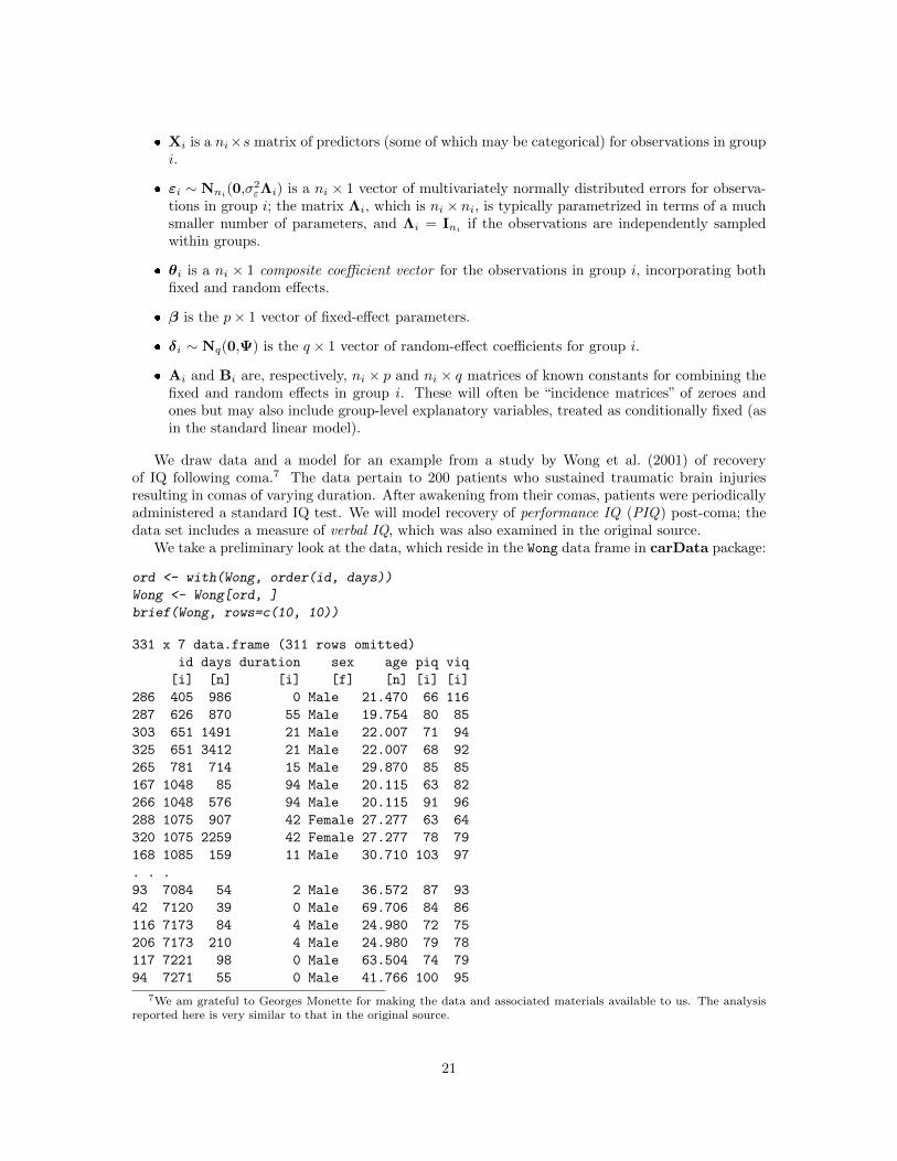
We draw data and a model for an example from a study by Wong et al. (2001) of recoveryof IQ following coma.7 The data pertain to 200 patients who sustained traumatic brain injuriesresulting in comas of varying duration. After awakening from their comas, patients were periodicallyadministered a standard IQ test. We will model recovery of performance IQ (PIQ) post-coma; thedata set includes a measure of verbal IQ, which was also examined in the original source.

We take a preliminary look at the data, which reside in the Wong data frame in carData package:

ord <- with(Wong, order(id, days))

Wong <- Wong[ord, ]

brief(Wong, rows=c(10, 10))


id days duration sex age piq viq

[i] [n] [i] [f] [n] [i] [i]

286 405 986 0 Male 21.470 66 116

287 626 870 55 Male 19.754 80 85

303 651 1491 21 Male 22.007 71 94

325 651 3412 21 Male 22.007 68 92

265 781 714 15 Male 29.870 85 85

167 1048 85 94 Male 20.115 63 82

266 1048 576 94 Male 20.115 91 96

288 1075 907 42 Female 27.277 63 64

320 1075 2259 42 Female 27.277 78 79

168 1085 159 11 Male 30.710 103 97

. . .

93 7084 54 2 Male 36.572 87 93

42 7120 39 0 Male 69.706 84 86

116 7173 84 4 Male 24.980 72 75

206 7173 210 4 Male 24.980 79 78

117 7221 98 0 Male 63.504 74 79

94 7271 55 0 Male 41.766 100 95

7We am grateful to Georges Monette for making the data and associated materials available to us. The analysisreported here is very similar to that in the original source.

21

43 7309 31 0 Female 50.667 85 95

44 7321 23 0 Male 26.004 84 83

95 7371 55 1 Male 56.786 80 88

45 7548 31 0 Male 24.367 108 106

nrow(Wong)

[1] 331

patients <- unique(with(Wong, id))

length(patients)

[1] 200

table(xtabs(~id, data=Wong))

1 2 3 4 5

107 61 27 4 1

with(Wong, sum(days > 1000))

[1] 40

plot(piq ~ days, xlab="Days Post Coma",

ylab="PIQ", xlim=c(0, 1000),

data=Wong, subset = days <= 1000)

for (patient in patients){

with(Wong, lines(days[id==patient], piq[id == patient], col="gray"))

}

with(Wong, lines(lowess(days, piq), lwd=2, col="darkblue"))

The variable id records patient number; days, the days post-recovery at which the IQ measurmentswere taken; duration, the length in days of the coma; and piq, the measured performance IQ of thepatient. The other variables, sex, age, and viq won’t enter our analysis and are self-explanatory.We sort the data by patient id and days within patients. Sorting isn’t necessary for fitting amixed-effects model to the data, but helps us to draw graphs of the data.8

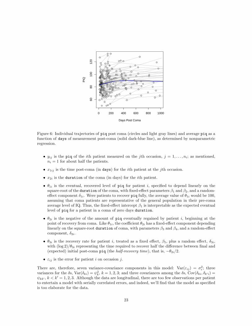
About half of the patients in the study (107) completed a single IQ test, but the remainder weremeasured on two to five irregularly timed occasions, raising the possibility of tracing the trajectoryof IQ recovery post-coma. A mixed-effects model is very useful here because it allows us to poolthe information in the small number of observations available per patient to estimate the typicalwithin-subject trajectory of recovery along with variation in this trajectory. The data are graphedin Figure 6, which shows the individual patients’ piq trajectories post-coma along with an averagetrajectory computed by the lowess() nonparametric-regression function. This graph is a scatterplotof piq versus number of days post-coma at the time of measurement, with the observations for eachpatient connected by lines. Forty of the 331 measurements were taken after 1000 days post-coma,and these are omitted from the graph to allow us to discern more clearly the general pattern of thedata.

After examining the data, Wong et al. (2001) posited an asymptotic growth model for IQ recovery:

yij = θ1i + θ2ie−θ3ix1ij + εij (4)

θ1i = β1 + β2√x2i + δ1i

θ2i = β3 + β4√x2i + δ2i

θ3i = β5 + δ3i

where the variables and parameters of the model have the following interpretations:

8Actually, the Wong.txt data file is effectively presorted within patients, and so this step isn’t strictly necessary.

22

0 200 400 600 800 1000

6080

100

120

Days Post Coma

PIQ

Figure 6: Individual trajectories of piq post coma (circles and light gray lines) and average piq as afunction of days of measurement post-coma (solid dark-blue line), as determined by nonparametricregression.

� yij is the piq of the ith patient measured on the jth occasion, j = 1, . . . , ni; as mentioned,ni = 1 for about half the patients.

� x1ij is the time post-coma (in days) for the ith patient at the jth occasion.

� x2i is the duration of the coma (in days) for the ith patient.

� θ1i is the eventual, recovered level of piq for patient i, specified to depend linearly on thesquare-root of the duration of the coma, with fixed-effect parameters β1 and β2, and a random-effect component δ1i. Were patients to recover piq fully, the average value of θ1i would be 100,assuming that coma patients are representative of the general population in their pre-comaaverage level of IQ. Thus, the fixed-effect intercept β1 is interpretable as the expected eventuallevel of piq for a patient in a coma of zero days duration.

� θ2i is the negative of the amount of piq eventually regained by patient i, beginning at thepoint of recovery from coma. Like θ1i, the coefficient θ2i has a fixed-effect component dependinglinearly on the square-root duration of coma, with parameters β3 and β4, and a random-effectcomponent, δ2i.

� θ3i is the recovery rate for patient i, treated as a fixed effect, β5, plus a random effect, δ3i,with (log 2)/θ3i representing the time required to recover half the difference between final and(expected) initial post-coma piq (the half-recovery time), that is, −θ2i/2.

� εij is the error for patient i on occasion j.

There are, therefore, seven variance-covariance components in this model: Var(εij) = σ2ε ; three

variances for the δs, Var(δki) = ψ2k, k = 1, 2, 3; and three covariances among the δs, Cov(δki, δk′i) =

ψkk′ , k < k′ = 1, 2, 3. Although the data are longitudinal, there are too few observations per patientto entertain a model with serially correlated errors, and indeed, we’ll find that the model as specifiedis too elaborate for the data.

23

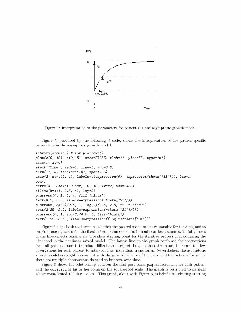
0 Time

PIQ

0

θ1i

− θ2i

− θ2i 2

(log 2) θ3i

Figure 7: Interpretation of the parameters for patient i in the asymptotic growth model.

Figure 7, produced by the following R code, shows the interpretation of the patient-specificparameters in the asymptotic growth model:

library(sfsmisc) # for p.arrows()

plot(c(0, 10), c(0, 5), axes=FALSE, xlab="", ylab="", type="n")

axis(1, at=0)

mtext("Time", side=1, line=1, adj=0.9)

text(-1, 5, labels="PIQ", xpd=TRUE)

axis(2, at=c(0, 4), labels=c(expression(0), expression(theta["1i"])), las=1)

box()

curve(4 - 3*exp(-0.5*x), 0, 10, lwd=2, add=TRUE)

abline(h=c(1, 2.5, 4), lty=2)

p.arrows(0, 1, 0, 4, fill="black")

text(0.5, 3.5, labels=expression(-theta["2i"]))

p.arrows(log(2)/0.5, 1, log(2)/0.5, 2.5, fill="black")

text(2.25, 2.0, labels=expression(-theta["2i"]/2))

p.arrows(0, 1, log(2)/0.5, 1, fill="black")

text(1.25, 0.75, labels=expression((log~2)/theta["3i"]))

Figure 6 helps both to determine whether the posited model seems reasonable for the data, and toprovide rough guesses for the fixed-effects parameters. As in nonlinear least squares, initial guessesof the fixed-effects parameters provide a starting point for the iterative process of maximizing thelikelihood in the nonlinear mixed model. The lowess line on the graph combines the observationsfrom all patients, and is therefore difficult to interpret, but, on the other hand, there are too fewobservations for each patient to establish clear individual trajectories. Nevertheless, the asymptoticgrowth model is roughly consistent with the general pattern of the data, and the patients for whomthere are multiple observations do tend to improve over time.

Figure 8 shows the relationship between the first post-coma piq measurement for each patientand the duration of his or her coma on the square-root scale. The graph is restricted to patientswhose coma lasted 100 days or less. This graph, along with Figure 6, is helpful in selecting starting

24

values for the model parameters.

Wong.first <- aggregate(Wong[, c("piq", "duration", "days")],

by=list(id=Wong$id), function(x) x[1])

Wong.first <- subset(Wong.first, duration <= 100)

brief(Wong.first)


id piq duration days

[i] [i] [i] [n]

1 405 66 0 986

2 626 80 55 870

3 651 71 21 1491

. . .

199 7371 80 1 55

200 7548 108 0 31

plot(piq ~ sqrt(duration), data=Wong.first,

xlab="Days in Coma (square-root scale)", ylab="Initial PIQ",

axes=FALSE, frame=TRUE)

axis(2)

axis(1, at=sqrt(c(0, 5, 10, seq(20, 100, by=20))),

labels=c(0, 5, 10, seq(20, 100, by=20)))

(mod.ag <- lm(piq ~ sqrt(duration), data=Wong.first))

Call:

lm(formula = piq ~ sqrt(duration), data = Wong.first)

Coefficients:

(Intercept) sqrt(duration)

88.49 -1.93

abline(mod.ag, lwd=2, lty=2)

with(Wong.first,

lines(lowess(sqrt(duration), piq), lwd=2, col="darkblue"))

We use the aggregate() function to create a data set that contains the first piq score for eachpatient, along with the patient’s duration of coma and the days post-coma at the first IQ measure-ment, and then limit the data set to durations of 100 days or less. The first measurement for eachpatient was never taken immediately upon recovery from coma (i.e., at days = 0), complicatinginterpretation, but our purpose is to get roughly reasonable start values for the parameters.

� Figure 6 leads us to expect that the average eventual level of recovered piq will be less than100, but Figure 8 also suggests that the average initial and hence eventual level for those whospent fewer days in a coma should be somewhat higher. We therefore use the start valueβ1 = 100.

� The slope of the least-squares line in Figure 8, relating initial piq to the square-root of dura-tion of coma, is −1.9, and thus we take β2 = −2.

� The parameter β3 represents the negative of the expected eventual gain in piq for a patientwho spent zero days in a coma. On the basis of the graphs, we guess that such patients starton average at a piq of 90 and eventually recover to an average of 100, suggesting the startvalue β3 = −10.

25

Days in Coma (square−root scale)

Initi

al P

IQ

6080

100

120

0 5 10 20 40 60 80 100

Figure 8: Scatterplot of initial piq for each patient versus duration of coma. The black broken lineis the least-squares line, the solid dark blue line is a nonparametric-regression smooth.

� The parameter β4 represents the change in expected eventual piq gain with a one-unit increasein the duration of the coma on the square-root scale. Our examination of the data does notprovide a basis for guessing the value of this parameter, and so we take β4 = 0.

� Recall that the time to half-recovery is (log 2)/β5. From Figure 6, it seems reasonable to guessthat the half-recovery time is around 100 days. Thus, β5 = (log 2)/100 = 0.007.

With the start values in hand, we call nlme() to fit the model:9

piq.mod.1 <- nlme(piq ~ theta1 + theta2*exp(-theta3*days), data=Wong,

fixed=list(

theta1 ~ 1 + sqrt(duration),


theta3 ~ 1),

random=list(id = list(theta1 ~ 1, theta2 ~ 1, theta3~1)),

start=list(fixed=c(100, -2, -10, 0, 0.007)),

control=nlmeControl(msMaxIter=500))

Warning in nlme.formula(piq ~ theta1 + theta2 * exp(-theta3 * days), data = Wong:

Iteration 3, LME step: nlminb() did not converge (code = 1).

PORT message: function evaluation limit reached without convergence (9)

Warning in nlme.formula(piq ~ theta1 + theta2 * exp(-theta3 * days), data = Wong:

Singular precision matrix in level -1, block 1

The specification of the model follows the general nonlinear mixed model in Equation 3 (page 20).Unlike for linear mixed models fit by lme(), the structure of the model is specified hierarchically.

9The default method in nlme() for fitting nonlinear mixed models is maximum likelihood, obtained explicitlyby the argument method="ML". Alternatively, we can fit by method="REML", but that proves even more unstablefor this problem. We invite the reader to refit the final model by REML, say piq.mod.3r <- update(piq.mod.3,

method="REML"), and compare the results.

26

The first (formula) argument is expressed in terms of patient-specific coefficients and is similar tothe formula for a nonlinear regression model fit by nls() (see Section ??). The fixed argumentspecifies relationships between the subject-specific coefficients and subject-level characteristics, hereduration. The random argument specifies the random-effect structure of the model, which is herejust a random error associated with each subject-specific coefficient, allowing these coefficients tovary by subject.

There are numerical problems in fitting this model, and so we consider simpler random-effectsstructures by successively removing δ3 and δ2 from the model:


fixed=list(



theta3 ~ 1),

random=list(id = list(theta1 ~ 1, theta2 ~ 1)),

start=list(fixed=c(100, -2, -10, 0, 0.007)))

Warning in nlme.formula(piq ~ theta1 + theta2 * exp(-theta3 * days), data = Wong,:


Do increase 'msMaxIter'!

Warning in nlme.formula(piq ~ theta1 + theta2 * exp(-theta3 * days), data = Wong,:


Do increase 'msMaxIter'!


fixed=list(



theta3 ~ 1),

random=list(id = list(theta1 ~ 1)),

start=list(fixed=c(100, -2, -10, 0, 0.007)))

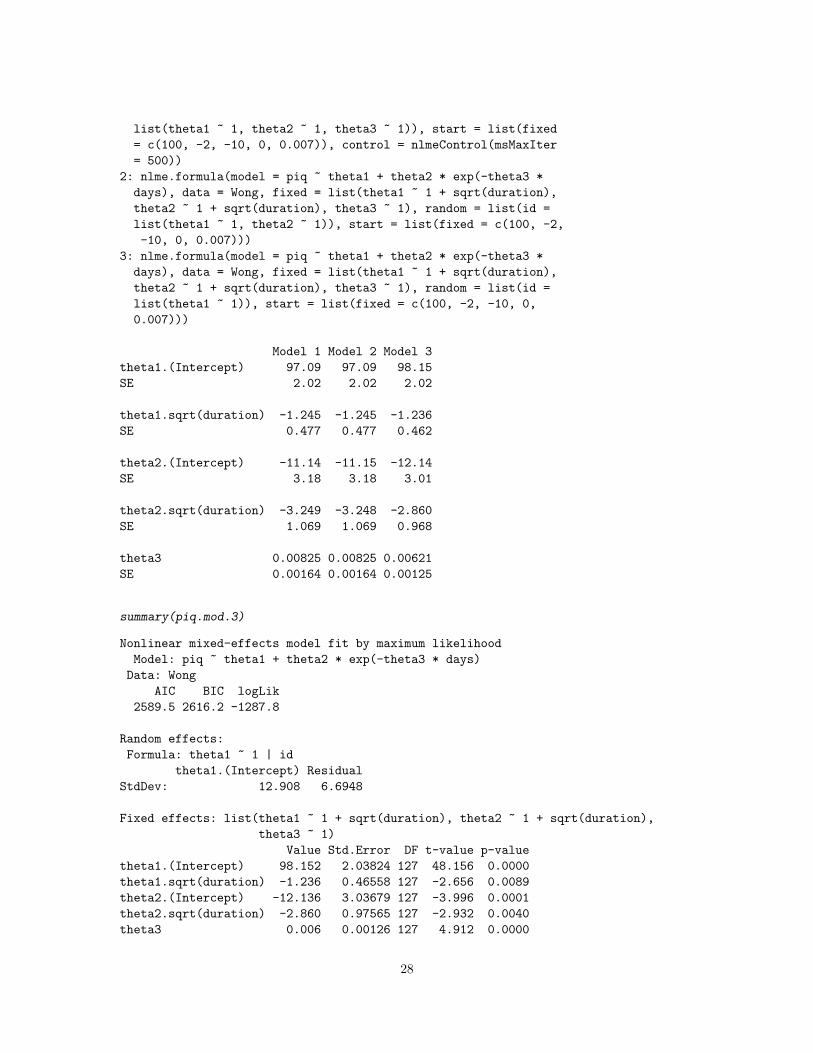
Only the simplest model, piq.mod.3, fits without difficulty. Likelihood-ratio tests, AIC, and BICsuggest that there’s no reason to prefer the more complex models:

anova(piq.mod.1, piq.mod.2, piq.mod.3)

Model df AIC BIC logLik Test L.Ratio p-value

piq.mod.1 1 12 2599.4 2645.0 -1287.7

piq.mod.2 2 9 2593.4 2627.6 -1287.7 1 vs 2 0.002278 1.0000

piq.mod.3 3 7 2589.5 2616.2 -1287.8 2 vs 3 0.185001 0.9116

The LR tests compare each model to the one immediately above it. Moreover, as is frequently thecase, the fixed-effect estimates are quite similar for the three random-effect specifications, even withconvergence problems apparent in fitting the models:

compareCoefs(piq.mod.1, piq.mod.2, piq.mod.3)

Calls:

1: nlme.formula(model = piq ~ theta1 + theta2 * exp(-theta3 *

days), data = Wong, fixed = list(theta1 ~ 1 + sqrt(duration),

theta2 ~ 1 + sqrt(duration), theta3 ~ 1), random = list(id =

27

list(theta1 ~ 1, theta2 ~ 1, theta3 ~ 1)), start = list(fixed

= c(100, -2, -10, 0, 0.007)), control = nlmeControl(msMaxIter

= 500))




list(theta1 ~ 1, theta2 ~ 1)), start = list(fixed = c(100, -2,

-10, 0, 0.007)))




list(theta1 ~ 1)), start = list(fixed = c(100, -2, -10, 0,

0.007)))

Model 1 Model 2 Model 3

theta1.(Intercept) 97.09 97.09 98.15

SE 2.02 2.02 2.02

theta1.sqrt(duration) -1.245 -1.245 -1.236

SE 0.477 0.477 0.462

theta2.(Intercept) -11.14 -11.15 -12.14

SE 3.18 3.18 3.01

theta2.sqrt(duration) -3.249 -3.248 -2.860

SE 1.069 1.069 0.968

theta3 0.00825 0.00825 0.00621

SE 0.00164 0.00164 0.00125

summary(piq.mod.3)

Nonlinear mixed-effects model fit by maximum likelihood

Model: piq ~ theta1 + theta2 * exp(-theta3 * days)

Data: Wong

AIC BIC logLik

2589.5 2616.2 -1287.8

Random effects:

Formula: theta1 ~ 1 | id

theta1.(Intercept) Residual

StdDev: 12.908 6.6948

Fixed effects: list(theta1 ~ 1 + sqrt(duration), theta2 ~ 1 + sqrt(duration),

theta3 ~ 1)

Value Std.Error DF t-value p-value

theta1.(Intercept) 98.152 2.03824 127 48.156 0.0000

theta1.sqrt(duration) -1.236 0.46558 127 -2.656 0.0089

theta2.(Intercept) -12.136 3.03679 127 -3.996 0.0001

theta2.sqrt(duration) -2.860 0.97565 127 -2.932 0.0040

theta3 0.006 0.00126 127 4.912 0.0000

28

Correlation:

t1.(I) th1.() t2.(I) th2.()

theta1.sqrt(duration) -0.712

theta2.(Intercept) -0.584 0.444

theta2.sqrt(duration) 0.455 -0.443 -0.805

theta3 -0.352 0.009 0.128 -0.336

Standardized Within-Group Residuals:

Min Q1 Med Q3 Max

-3.067982 -0.375418 0.013861 0.375336 2.460507

Number of Observations: 331

Number of Groups: 200

Focusing then on model piq.mod.3, the average final level of recovered piq following a coma

of zero days is β̂1 = 98.15, and this level declines with the square-root duration of the coma atthe rate β̂2 = −1.236 points per square-root day (e.g., from day 1 to day 4 or from day 4 to day

9). On average, patients who spend zero days in coma recover −β̂3 = 12.14 piq points, and the

size of the recovery grows with the square-root duration of the coma, −β̂4 = 2.860. The estimatedhalf-recovery time is (log 2)/β̂5 = (log 2)/0.00621 = 112 days. We can use the delta method to geta standard error and confidence limits (which turn out to be wide) for this estimate:

deltaMethod(piq.mod.3, "log(2)/beta5", parameterNames=paste0("beta", 1:5))


log(2)/beta5 111.67 22.564 67.446 155.89

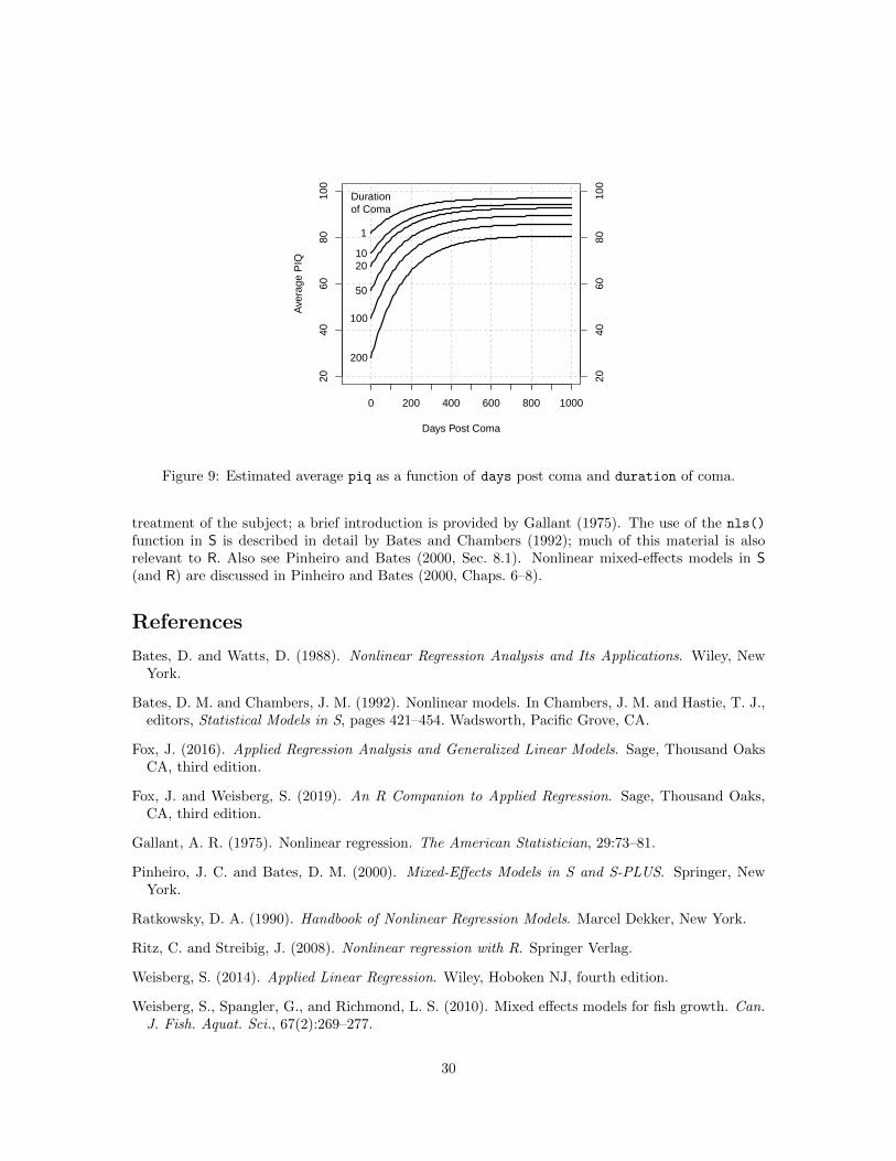
Figure 9 is a fixed-effect display for the model, similar to one that appears in Wong et al. (2001),showing estimated average piq as a function of duration of coma and days post coma:

newdata <- expand.grid(duration=c(1, 10, 20, 50, 100, 200),

days=seq(0, 1000, 20))

newdata$piq <- predict(piq.mod.3, newdata, level=0)

plot(piq ~ days, type="n", xlab="Days Post Coma", ylab="Average PIQ",

ylim=c(20, 100), xlim=c(-100, 1000), data=newdata, axes=FALSE, frame=TRUE)

axis(2) # left

axis(4) # right

axis(1, at=seq(0, 1000, by=100)) # bottom

grid(lty=2, col="gray")

for (dur in c(1, 10, 20, 50, 100, 200)){

with(newdata, {

lines(spline(seq(0, 1000, 20), piq[duration == dur]), lwd=2)

text(-25, piq[duration == dur][1], labels=dur, adj=0.9)

})

}

text(-100, 95, labels="Duration\nof Coma", adj=0)

9 Complementary Reading and References

Nonlinear regression and nonlinear least squares are discussed in Weisberg (2014, Chap. 11) and Fox(2016, Chap. 17), and in Ritz and Streibig (2008). Bates and Watts (1988) present a comprehensive

29

Days Post Coma

Ave

rage

PIQ

2040

6080

100

2040

6080

100

0 200 400 600 800 1000

1

1020

50

100

200

Durationof Coma

Figure 9: Estimated average piq as a function of days post coma and duration of coma.

treatment of the subject; a brief introduction is provided by Gallant (1975). The use of the nls()

function in S is described in detail by Bates and Chambers (1992); much of this material is alsorelevant to R. Also see Pinheiro and Bates (2000, Sec. 8.1). Nonlinear mixed-effects models in S(and R) are discussed in Pinheiro and Bates (2000, Chaps. 6–8).

References

Bates, D. and Watts, D. (1988). Nonlinear Regression Analysis and Its Applications. Wiley, NewYork.

Bates, D. M. and Chambers, J. M. (1992). Nonlinear models. In Chambers, J. M. and Hastie, T. J.,editors, Statistical Models in S, pages 421–454. Wadsworth, Pacific Grove, CA.

Fox, J. (2016). Applied Regression Analysis and Generalized Linear Models. Sage, Thousand OaksCA, third edition.

Fox, J. and Weisberg, S. (2019). An R Companion to Applied Regression. Sage, Thousand Oaks,CA, third edition.

Gallant, A. R. (1975). Nonlinear regression. The American Statistician, 29:73–81.

Pinheiro, J. C. and Bates, D. M. (2000). Mixed-Effects Models in S and S-PLUS. Springer, NewYork.

Ratkowsky, D. A. (1990). Handbook of Nonlinear Regression Models. Marcel Dekker, New York.

Ritz, C. and Streibig, J. (2008). Nonlinear regression with R. Springer Verlag.

Weisberg, S. (2014). Applied Linear Regression. Wiley, Hoboken NJ, fourth edition.

Weisberg, S., Spangler, G., and Richmond, L. S. (2010). Mixed effects models for fish growth. Can.J. Fish. Aquat. Sci., 67(2):269–277.

30

Wong, P. P., Monette, G., and Weiner, N. I. (2001). Mathematical models of cognitive recovery.Brain Injury, 15:519–530.

31

Documents

Nonlinear Regression, Nonlinear Least Squares, and ...change a nonlinear relationship into a linear one (in these data, replacing population by its cube-root linearizes the plot, as