An International Journal

computers & mathematics with applicatloM

PERGAMON Computers and Mathematics with Applications 45 (2003) 1059-1073 www.elsevier.nl/locate/camwa

Normal Forms for Nonautonomous Difference Equations

S. SIEGMUND Department of Mathematics

University of California Berkeley, CA 94720, U.S.A.

siegmund&nath.berkeley.edu

Abstract-we extend Henry Poincare’s normal form theory for autonomous difference equations "k+l = f(xk) to nonautonomous difference equations zk+r = fk(zk). Poincare’s nonresonance condition Xj - nz, Xpi # 0 for eigenvalues is generalized to the new nonresonance condition Xj n nbl Xy = 0 for spectral intervals. @ 2003 Elsevier Science Ltd. All rights reserved.

Keywords-Poincare normal form theory, Nonautonomous normal forms, Resonance, Nonau- tonomous difference equations.

1. INTRODUCTION

The famous French mathematician Henry Poincare founded the normal form theory for au- tonomous differential equations j. = f( x near a rest point in his thesis in 1879. Soon a parallel ) theory for autonomous difference equations xk+i = f(xk) was developed. If the eigenvalues Xl,... ,X, of the linearization xk+i = Df(x’)xk at the rest point x0 satisfy the nonresonance condition

xj #x;l...x~, (1)

j E (1,. . . ) n}, qi E NO = {O,l,. . . }, Cy=“=, qi 2 2, then the difference equation can be formally linearized.

As an example, we consider the following planar autonomous system:

xk+l = 2xk,

Yk+l = xyk + &

with A E (0, oo). We are looking for a near-identity transformation

H(x, y) = ; + h2(X,Y), 0

which eliminates the second order nonlinearity (,“2) an d we choose hz E span{(f), (s), (y), (,“,), (“,a), ($)}. It is not difficult to show that the transformed equation has no second-order nonlin- earity if and only if the so-called homological equation

= f2(? Y)

08981221/03/$ - see front matter @ 2003 Elsevier Science Ltd. All rights reserved. Typeset by dM-l’$$ PII: SO898-1221(03)00085-3

1060 S. SIEGMUND

is satisfied with

and fibc,~)= (3

It is solvable if and only if X # 4 and with its unique solution we get

X

H(X,Y) = ( ) 1 * -x2

y+A-4

In this simple example, the transformed equation xk+i = 2xk, yk+r = k& is linear. In general, the elimination of second-order nonlinearities produces higher-order nonlinearities, and the process has to be iterated. The resulting transformation is the composition of the transformations of each elimination step, and it is nonlinear but is constructed by solving a sequence of linear equations.

In this article, we consider nonautonomous invertible difference equations

Xk+l = fk(2k) (2)

not in the vicinity of a rest point as Poincare did it in the autonomous case, but in the vicinity of an arbitrary reference solution w” : z + RN. For some p 2 2 we assume fk : Df, C

RN -t fk(Dfk) c RN to be a 0’ diffeomorphism for every k E Z = (0, fl, . . . }. We will extend Poincare’s normal form theory by showing that if the linearization xk+r = Dfk($)xk of (2) along the reference solution v” has invertible coefficient matrices Dfk(vg) E BNX N, k E Z, and satisfies a nonresonance condition, then system (2) is locally 0’ equivalent to a system xk+l = gh(xk) in normal form; i.e., with zero reference solution, block diagonal linear part xk+l = Dgk(O)xk and all nonresonant Taylor coefficients of g up to order p are zero.

We therefore have to use a proper replacement of the “linear algebra” for autonomous systems (i.e., eigenvalues and eigenspaces) in our nonautonomous situation. A spectral theory for nonau- tonomous difference equations is developed in [l]. The dichotomy spectrum of the linearized difference equation xk+i = Dfk(vi)xk consists of at most N closed intervals of the positive real line Wf = (0, co); in general, the spectrum may be empty or unbounded. It is nonempty and compact, i.e., consists of n compact intervals with 1 5 n 5 N, if the system has bounded growth. A linear system xk+l = Akxk has bounded growth if its evolution operator @ satisfies the esti- mate ll@(k,l)ll 5 Ku Ikeel for k, e E Z with constants K, a 1 1. Bounded growth is equivalent to the boundedness of the coefficients and their inverses [l, Lemma 2.31, and hence, the linearized difference equation xk+l = Dfk($!)Xk has bounded growth if ]]&]I 5 kf and llAk’/l 5 M for k E Z with some constant M 2 0 and Ak = Dfk(vi).

For simplicity, we assume in the following that the linearized equation has bounded growth, although the theory could also be developed in the general case.

2. PRELIMINARIES

Let d(- ; C t) : Ie,c + RN denote the uniq ue maximal solution of the initial value problem (2), xe = < for E E Df, where It,< is a Z-interval (i.e., an intersection of an interval with Z) containing f? such that the solution identity

4(k + 1; 6 8 = fk(d(k e, t)), for k, k + 1 E It,<,

holds. We have q5(-$ e, 6) = [ and d(k; 4(m; -t, f)) = $(k + m; !, t) for m, k + m E Ie,<. There is no straightforward way to define a notion of conjugacy for nonautonomous difference

equations. What do we mean by this? Two autonomous difference equations xk+i = f ‘(xk) and xk+i = f2(zk) in RN are said to be conjugate if there exists a homeomorphism H : RN + RN such that the flows &(e ;[), respectively, q52(.; 11) satisfy the conjugacy relation H(&(k;e)) = &(k;H([)) for all t E RN, k E IE; i.e., H maps solutions of the first equation onto solutions of

Nonautonomous Difference Equations 1061

the second equation and vice versa for H- l. Now if we would define a conjugacy between two nonautonomous difference equations zk+l = fJ(zk) and X&l = fi(zk) by the same property, but now with a k-dependent H, then for every C E Ik,r

&c(X) := h(k; l, 4l(C k, x))

would establish a conjugacy; i.e., H maps solutions of the first equation onto solutions of the second equation and vice versa with

H,y’(x) := 4l(k;C4$;k,x)).

In the nonautonomous situation, we need, therefore, some additional conditions which ensure that qualitative behaviour-at least for a single reference solution-is preserved under the trans- formation.

It is easy to see in the autonomous situation that for a conjugacy, periodic solutions, limit sets, and invariant sets of the first equation are bijectively mapped onto periodic solutions, limit sets, and invariant sets, respectively, of the second equation and that (asymptotic) stability, attractivity, and instability of bounded solutions are preserved under the conjugacy. In most cases this is enough, but note that the assumption of boundedness of solutions is essential for the preservation of stability. For example: the two linear systems xk+l = xk + 1, Yk+l = (1/2)yk and z&l = ICY + 1, yk+l = !& are conjugate via H(x, y) = (z,$~~), but the first system is stable and the second is unstable. To preserve the stability of an unbounded solution vk, it would be necessary to pose some uniformity condition on H, e.g., limz.+o H(vk + z) = H(vk) uniformly in k E Z. Such a uniformity condition is exactly what we need in the nonautonomous situation to define a meaningful notion of 0’ equivalence.

Consider difference equations together with reference solutions

xk+l = fk(ek)r v” :Z+RN, (3)

z/c+1 = gk(xk)r wO:Z+RN, (4

where fk and gk are 0’ diffeomorphisms, i.e., .fk E Diffp(Df,, fk(Dfr)), gk E DiffP(D,,,gk(ogk)), p > 0. We assume that uniform neighbourhoods of the reference solutions are contained in the corresponding sets of definition, i.e., there exist E > 0 and S > 0 such that

J% (WE) c Df, and Bs (WE) c D,, , for k E Z,

where BE(xo) := {x E RN : 11x - x011 < E}. Define UE(vo) := {(k,x) E Z x RN : z E BE(vg)}.

DEFINITION 1. Consider systems (3) and (4). If there exist E’, 6’ with 0 < E’ 5 E and 0 < b’ 5 b together with functions

H : U&I”) -+ RN, H-l : U&I (w’) -+ RN,

then H is called a local CP equivalence between system (3) with solution v” and system (4) with solution w”, if the following statements are valid.

(A) For each k E Z, the mappings

Hk : B,, (WE) + Hk (Be (u;)) C Bs (‘WE) ,

H,-’ : B&t (w;) + H; ’ (BP (w:)) c B, ($$

are 0’ diffeomorphisms (or homeomorphisms if p = 0) with

&(&l(x)) = x and H;‘(Hk(x)) = x

for all x for which the compositions are defined.

1062 S. SIEGMUND

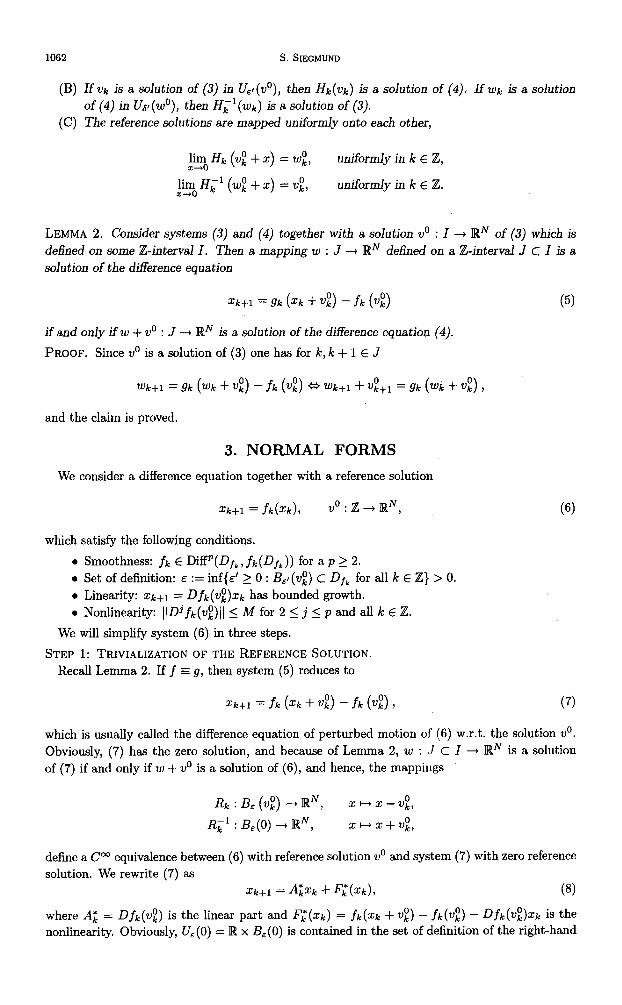
(B) If vk is a solution of (3) in UEl(vo), then I-I k vk is a Sohkn of (4). If ?.L& is a solution ( ) Of (4) in up(W”), then Hi’(Wk) is a SdutiOn Of (3).

(C) The reference solutions are mapped uniformly onto each other,

;FoHk (Vi +Z) = W;,

liio I?,-’ (wi + x) = vi,

uniformly in k E Z,

uniformly in k E Z.

LEMMA 2. Consider systems (3) and (4) together with a solution v” : I --t RN of (3) which is defined on some Z-interval I. Then a mapping w : J --) RN defined on a Z-interval J c I is a solution of the difference equation

zk+l = gk (ek + vi) - fk (Vi) (5)

ifandonlyifw+v’: J-+WN is a solution of the difference equation (4).

PROOF. Since v” is a solution of (3) one has for k, k + 1 E J

wk+l = gk (wk + Vi) - fk (Vi) * wk+l+v:+l = gk(Wi + Vi),

and the claim is proved.

3. NORMAL FORMS We consider a difference equation together with a reference solution

xk+l = fk(zk), v" : z + RN, (6)

which satisfy the following conditions.

l Smoothness: fk E DiffP(Dfk, fk(D&)) for a p 2 2. l Set of definition: E := inf{$ 2 0 : &(v~) c Df, for all k E Z} > 0. l Linearity: xk+l = Dfk(v$xk has bounded growth. l Nonlinearity: II@fk(vg)II 5 M for 2 5 j 5 p and all k E Z.

We will simplify system (6) in three steps.

STEP 1: TRIVIALIZATION OF THE REFERENCE SOLUTION. F&call Lemma 2. If f E g, then system (5) reduces to

xk+l = fk (xk + v,$ - fk (vi) , (7)

which is usually called the difference equation of perturbed motion of (6) w.r.t. the solution v”. Obviously, (7) has the zero solution, and because of Lemma 2, w : .I c I + RN is a solution of (7) if and only if w + v” is a solution of (6), and hence, the mappings

Rk : & (71;) -+ RN, x H x -vi,

Ril : BE(O) -+ RN, xcx+v;,

define a C” equivalence between (6) with reference solution v” and system (7) with zero reference solution. We rewrite (7) as

Xk+l = A;% + $(xk), (8)

where A; = Dfk (v:) is the linear part and &?(xk) = fk(xk + vi) - fk(Vz) - Dfk(Vi)Xk is the nonlinearity. Obviously, U, (0) = R x BE(O) is contained in the set of definition of the right-hand

Nonautonomous Difference Equations 1063

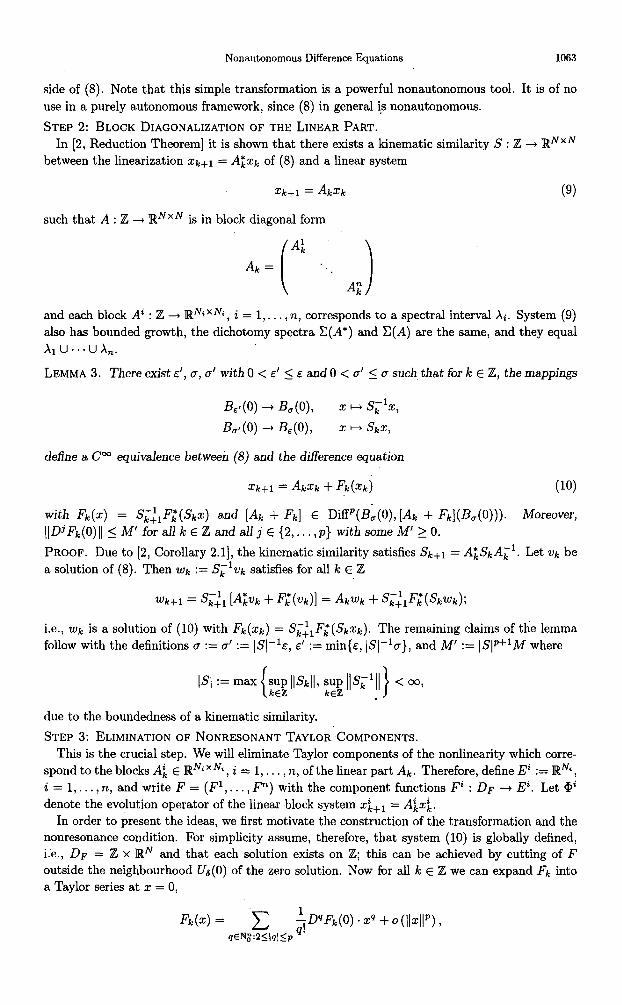
side of (8). Note that this simple transformation is a powerful nonautonomous tool. It is of no use in a purely autonomous framework, since (8) in general is nonautonomous.

STEP 2: BLOCK DIAGONALIZATION OF THE LINEAR PART. In [2, Reduction Theorem] it is shown that there exists a kinematic similarity S : Z --+ WNX N

between the linearization ~k+l = A& of (8) and a linear system

xk+l = AkXk (9)

such that A : Z + RNX N is in block diagonal form

4 A,, = i I

. . 4

and each block Ai : Z -+ WNix Ni, i = 1 , . . . , n, corresponds to a spectral interval Xi. System (9) also has bounded growth, the dichotomy spectra C(A*) and C(A) are the same, and they equal Xl u . . . u A,.

LEMMA 3. There exist E’, (T, (r’ with 0 < E’ 5 E and 0 < C’ 5 u such that for k E Z, the mappings

define a C” equivalence between (8) and the difference equation

Zk+l = AkXk + Fk(%kj (10)

with F&) = s&F;(s@) and [Ak + Fk] E Diff’(Bb(O), [Ak + Fk](B,(O))). Moreover, IlojFk(O)ll 5 M’ for all k E Z and aI1 j E (2,. . . ,p} with some M’ 2 0. PROOF. Due to [2, Corollary 2.11, the kinematic similarity satisfies sk+l = A;skAil. Let ?& be a solution of (8). Then ‘wk := sil?& satisfies for all k E Z

wk+l = s,& [A;Vk + &+(vk)] = AkWk + s$F;(skWk);

i.e., Wk iS a solution Of (10) with Fk(xk) = SiilFc(S@&). The remahing claims of the lemma follow with the definitions ~7 := 0 := JS(-l~, E’ := min{&, JSI-la}, and M’ := ISlp+lM where

due to the boundedness of a kinematic similarity.

STEP 3: ELIMINATION OF NONRESONANT TAYLOR’COMPONENTS. This is the crucial step. We will eliminate Taylor components of the nonlinearity which corre-

spondtotheblocksAkEIWNixNi,i=l,... , n, of the linear part Ah. Therefore, define Ei := RN;, i=l , . . . ,n, and write F = (Fl,. . . , F”) with the component functions Fi : DF + E’. Let @’ denote the evolution operator of the linear block system x:+~ = Aix:.

In order to present the ideas, we first motivate the construction of the transformation and the nonresonance condition. For simplicity assume, therefore, that system (10) is globally defined, i.e., DF = iZ x RN and that each solution exists on Z; this can be achieved by cutting of F outside the neighbourhood Us(O) of the zero solution. Now for all k E Z we can expand Fk into a Taylor series at x = 0,

F/c(x) = -c -$Dq&(0) . x4 + fJ (1141”) 7 s~r”r,-:21lql<P .

1064 S. SIEGMUND

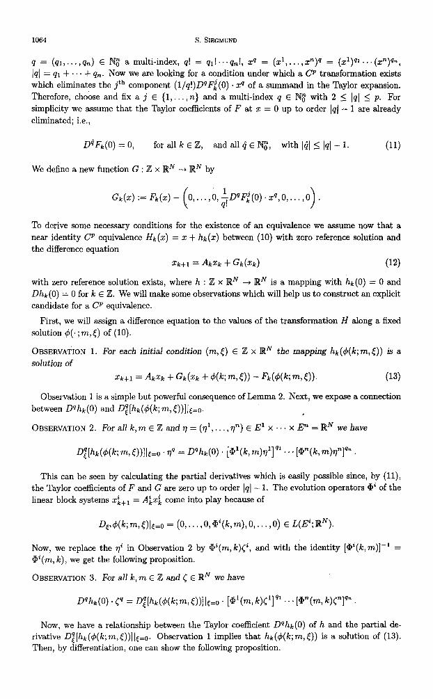
q = (41,. . . ,qn) E IV: a multi-index, q! = ql! ... q,,!, 29 = (d, . . . ,zn)q = (x1)91 . . . (cP)qn, IQI = 41 f... + qn. Now we are looking for a condition under which a 0’ transformation exists which eliminates the jth component (l/q!)DQFl(O) . ZQ of a summand in the Taylor expansion. Therefore, choose and fix a j E (1, . . . ,n} and a multi-index q E N2; with 2 5 141 5 p. For simplicity we assume that the Taylor coefficients of F at 2 = 0 up to order 1q( - 1 are already eliminated; i.e.,

DQFk(0) = 0, for all Ic E Z, and all 4 E Nz, with 141 5 141 - 1. (11)

We define a new function G : Z x RN --+ RN by

G,(x) := F/&T) - x4,0,. , , ,o >

.

To derive some necessary conditions for the existence of an equivalence we assume now that a near identity Cp equivalence Hk(z) = z + hk(z) between (10) with zero reference solution and the difference equation

zk+l = AkQ + Gk(Q) (12)

with zero reference solution exists, where h : Z x RN + RN is a mapping with hk(0) = 0 and Dhk(O) = 0 for k E Z. We will make some observations which will help us to construct an explicit candidate for a CP equivalence.

First, we will assign a difference equation to the values of the transformation H along a fixed solution d(.;m,[) of (10).

OBSERVATION 1. For each initial condition (m,<) E Z x RN the mapping hk($(k; m,t)) is a solution of

zk+l = h& + Gk(Q + +(k; m, t)) - Fk(+(k; m, 5)). (13)

Observation 1 is a simple but powerful consequence of Lemma 2. Next, we expose a connection between Dqhk(0) and Di[hk(4(k; m,[))]I+o. *

OBSERVATION 2. For all k, m E Z and 77 = (r]‘, . . . ,v”) E El x . . . x E” = RN we have

D;[h&b(k;m,[))]I+o . vq = D’hk(O) . [@l(k,+‘]q’ a** [Q”(k,~)rl”Iq”~

This can be seen by calculating the partial derivatives which is easily possible since, by (ll), the Taylor coefficients of F and G are zero up to order IqI - 1. The evolution operators Qd of the linear block systems ~i+r = A:xi come into play because of

+$(k; m,<)IE=o = (0,. . . ,O, @(k, m), 0,. . . 70) E L(Ei; RN).

Now, we replace the vi in Observation 2 by @(m, k)c, and with the identity [@(k,m)]-’ = @(m, k), we get the following proposition.

OBSERVATION 3. For all k,m E iz and C E RN we have

Dqhk(0) .Cq = DEQ[hk(~(k;m,~))]l~=o. [~l(~,k)C1]ql...[~n(~,k)C”lq”.

Now, we have a relationship between the Taylor coefficient Dqhk(0) of h and the partial de- rivative Dg[hk(4(k, . m, E))] ]~=c. Observation 1 implies that hk(d(k; m, t)) is a solution of (13). Then, by differentiation, one can show the following proposition.

Nonautonomous Difference Equations 1065

OBSERVATION 4. The function o,“[hk(4(k;m, t))]+~ is a solution of

x/c+1 = Am + ck,

the variational equation of (13) in Lq(E1, . . . , E”; RN), where

(14)

ck=- 0,s.. (

,o,Dq(o),o,. . . ,o >

. [ipl(k,m)]q’ . *. [vyk,m)]qn .

So far, we have assumed that a CP equivalence Hk(z) = z + hk(2) between (10) and (12) exists and by Observation 3, the Taylor coefficient (l/q!)D’hk(O) . xq is a function of a special solution Di[hk(+(k; m, c))]l.+c of the difference equation (14) and the known evolution operators @.

From now on, we want to use this information to construct a candidate for a CP equivalence between (10) and (12). We make the ansatz

&(x) = x + --D’hk(o) . x9; ,‘!

i.e., hk(x) = (l/q!)Dqhk(o). XQ has only one nontrivial Taylor coefficient. We make use of Observations 3 and 4 in the way that we choose a special solution z of (14)

and interpret Zk as o:[hk(f$(k; m, <))I JE=~ for an arbitrary but fixed m E Z. With Observation 3 and our ansatz, this yields

. Hk(x) =x-k $zk. [@l(m,k)X’]ql -.‘[+“(m,k)xn]qn. (15)

Which solution .z of (14) should we choose ? To satisfy the condition (C) of Definition 1, it is necessary that lirnZ+o Hk(X) = 0 uniformly in k E Z, and this is satisfied if Zk . [a1 (m, k).]ql . . . [an(m, Ic).]qn is bounded for k E Z. Using [2], one knows that the borders of the spectral intervals Xi = [ai,bi] yield the exponential growth rates of the evolution operators ai of x:+~ = Atxi. Now it is the exponential growth rate of z we have to take care of. Here a key lemma comes in Play.

LEMMA 8. Consider the jth component of (14)

xcjktl = Ajk2; + c$. (16)

(A) Assume that the spectral intervals Xi = [ai, bi] satisfy the condition

aj > bp’...bF. (17)

Choose a y E (b:’ . . . bg, aj). Then zi := - Czk @j(k,! + l)c$ is the unique solution of (16) with the exponential growth rate yk for k -+ 00, i.e., jlz;II < C’y” for all k 2 0 with some C’ 2 0.

(B) Assume the condition b. <+..@ (18)

Choose a y E (bj, @ * . . a? ). Td, 4 := &tm @(k, e + l)d is the unique solution of (16) with the exponential growth rate y” for k --t -oo.

PROOF. We prove only (A). For every E > 1 we get with [2, Corollary 3.11 a constant K > 1 with

5 MIe (by’ . . . b$&?l)e-m , for e 2 m,

(4’ ..-a~s-lql)e-m, for e 5 m.

The rest follows from [3, Lemma 3.41.

1066 S. SIEGMUND

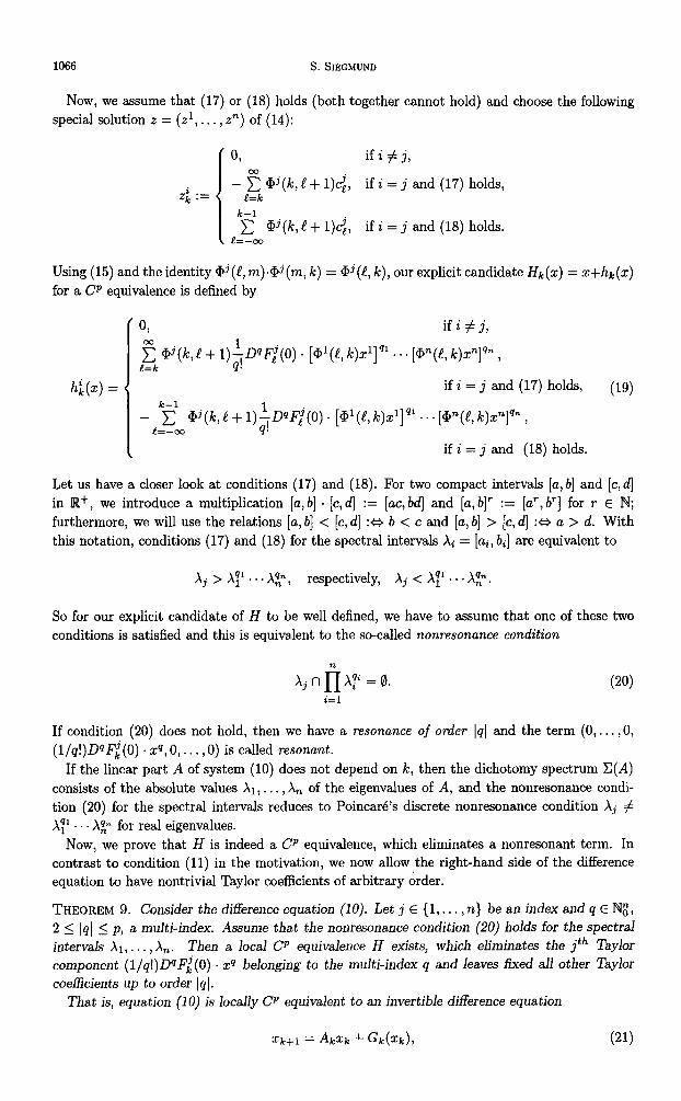
Now, we assume that (17) or (18) holds (both together cannot hold) and choose the following special solution z = (zl, . . . ,z”) of (14):

0, if i # j,

- 5 @(lc,C + l)d, if i = j and (17) holds, e=k

k-l c @(k,C + l)d, if i = j and (18) holds.

e=--oo

Using (15) and the identity @j (f?, m)@ (m, lc) = @j(f!, k), our explicit candidate Hk(x) = z+hk(z) for a CP equivalence is defined by

I 0, if i # j,

E @j(k,l+ l)+F:(o) . pyc, k)xl]Q1 *. . [@ye, k)xc”]Q” , e=k

h;(x) =

1

if i = j and (17) holds, (19) k-l

-e=C_~~(k,(+l)~DQ~~(0). [@‘(C,~)X’]‘~ +I?~(@)x~]~“,

if i = j and (18) holds.

Let us have a closer look at conditions (17) and (18). For two compact intervals [a, b] and [c, d] in W+, we introduce a multiplication [o,b] . [c,d] := [ac, bd] and [a, b]’ := [ur, b’] for r E NJ; furthermore, we will use the relations [a, b] < [c, d] :e b < c and [a, b] > [c, d] :e a > d. With this notation, conditions (17) and (18) for the spectral intervals Xi = [ai, bi] are equivalent to

Xj > Xyl * * . A:, respectively, Xj < XT1 . . . A:.

So for our explicit candidate of H to be well defined, we have to assume that one of these two conditions is satisfied and this is equivalent to the so-called nonresonance condition

AjflfiAy =0. (20) i=l

If condition (20) does not hold, then we have a resonance of order 141 and the term (0,. . . ,O, (l/q!)DF~(O) . xQ, 0,. . . ,0) is called resonant.

If the linear part A of system (10) does not depend on k, then the dichotomy spectrum C(A) consists of the absolute values Xi, . . . ,X, of the eigenvalues of A, and the nonresonance condi- tion (20) for the spectral intervals reduces to Poincare’s discrete nonresonance condition Xj # x71 . . . Xe for real eigenvalues.

Now, we prove that H is indeed a CP equivalence, which eliminates a nonresonant term. In contrast to condition (11) in the motivation, we now allow the right-hand side of the difference equation to have nontrivial Taylor coefficients of arbitrary order.

THEOREM 9. Consider the difference equation (10). Let j E { 1,. . . , n} be an index and q E NE, 2 5 141 < p, a multi-index. Assume that the nonresonance condition (20) holds for the spectral intervals Xi,. . . ,X,. Then a local CP equivalence H exists, which eliminates the jt” TayJor component (l/q!)DQFkj(O) . xQ belonging to the multi-index q and leaves fixed all other Taylor coefficients up to order 141.

That is, equation (10) is locally CP equivalent to an invertible difference equation

xk+l = AkXk + Gk(Vc), (21)

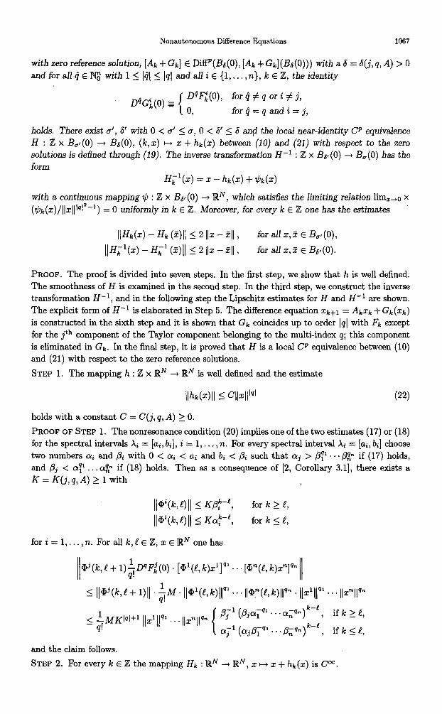
Nonautonomous Difference Equations 1067

with zero reference solution, [Ak + Gk] E DiP(&(O), [Ak + Ck](&(O))) with a 6 = b(j, q, A) > 0 and for all 4 E NG with 1 5 141 5 (41 and all i E (1,. . . , n}, k E Z, the identity

for 4 # q or i # j,

for 4 = q and i = j,

holds. There exist g’, 6’ with 0 < u’ 5 u, 0 < 6’ 2 6 an+ the local near-identity CP equivalence H : Z x B,,(O) + B&(O), (k, ) z H 2 + hk(z) between (10) and (21) with respect to the zero solutions is defined through (19). The inverse transformation H-l : Z x Bg,(O) + Bb(0) has the form

Hil(x) = x - h/c(x) + @k(x)

with a continuous mapping II, : Z x Bgj (0) + RN, which satisfies the limiting relation limZ+o x ($k(x)/IIx[I’q’a-l) = 0 uniformly in k E Z. Moreover, for every k E Z one has the estimates

lb%(x) - Hk @)I1 I 2 1(x - 311, for all x, 5 E B,,(O),

/HF’(x) - HL1 (?)I( 5 2 112 - 211, for all z,f E Bp(0).

PROOF. The proof is divided into seven steps. In the first step, we show that h is well defined. The smoothness of H is examined in the second step. In the third step, we construct the inverse transformation H-l, and in the following step the Lipschitz estimates for H and H-’ are shown. The explicit form of H-l is elaborated in Step 5. The difference equation xk+l = &xk + Gk(Xk)

is constructed in the sixth step and it is shown that Ck coincides up to order 141 with Fk except for the jth component of the Taylor component belonging to the multi-index q; this component is eliminated in Ck. In the final step, it is proved that H is a local CP equivalence between (10) and (21) with respect to the zero reference solutions.

STEP 1. The mapping h : Z x RN + R N is well defined and the estimate

(22)

holds with a constant C = C(j, q, A) 2 0.

PROOF OF STEP 1. The nonresonance condition (20) implies one of the two estimates (17) or (18) for the spectral intervals Xi = [ai, bi], i = 1,. . . , n. For every spectral interval Xi = [ai, bi] choose two numbers cyi and /?i with 0 < (pi < ai and bi < /3i such that aj > /3? . . . /3? if (17) holds, and pj < a?...@ if (18) holds. Then as a consequence of [2, Corollary 3.11, there exists a K = K(j, q, A) 2 1 with

IJ@(k,Oll I Kpfe, for k 2 .&

Il@(k,C)II I Kafe, for k 5 .&

fori=l,..., n. Forallk,~EZ,xEWNonehss

I/ @(k,L + l)-+‘F;(O) . [@‘(e, k)xl]” . . . [P(fJ, k)xn]qnll

I ll@jW+ 1111 . . $M. 1191(1, k)jl” . . . @l”(l, k)ll”” . )lxlllql . . . llxnllQn

and the claim follows. STEP 2. For every k E Z the mapping Hk : RN + RN, x H z + hk(x) is Coo.

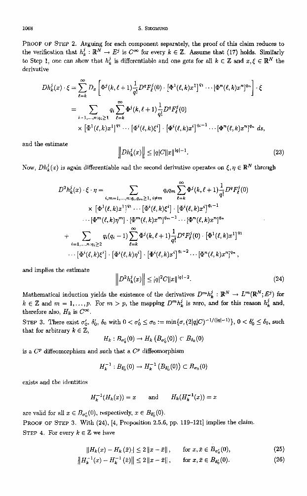
1068 S. SIEGMUND

PROOF OF STEP 2. Arguing for each component separately, the proof of this claim reduces to the verification that hi : RN + Ej is C”O for every k E Z. Assume that (17) holds. Similarly to Step 1, one can show that hi is differentiable and one gets for all k E Z and x,e E RN the derivative

Dhj&) . t = ED, [mj(k, C + l)$D’@(O) . [(a’(!, k)x’lql . . . [a)“([, k)i”l’.] . E e=k

x [@I(& k)xllq’ . . . [@(t, k)Ei] . [@(l, k)xi]q’-l . . . [+“(l, k)xnlq” ds,

and the estimate

IlDhjk(x)(l I IqlCl141’q’-‘. (23) Now, Oh:(x) is again differentiable and the second derivative operates on <, q E RN through

D2h;(x) . E. 77 = c i,m=l,..., n:qi,q,>l, i#m

qiqm 2 @(k,P + l);D’F’(O) e=k

x [@‘(t, k)xl]‘l . . . [@(!, k@] . [@(l, k)xilq’-’

. . + [@“(t, k)vn] . [@“(l, k)xm]qm-l . . . [@“(e, k)xnlqn

and implies the estimate

11D2h’k(x)l( I (q(2CJIxll’q’-2. (24)

Mathematical induction yields the existence of the derivatives D”hjk : RN + L”(R”; Ej) for kEZandm=l , . . . , p. For m > p, the mapping Dmhi is zero, and for this reason hi and, therefore also, Hk is Cm.

STEP 3. There exist CA, 66, 60 with 0 < uI, 5 a0 := min{a, (2/qlC)-1/(1qf-1)}, 0 < 66 5 60, such that for arbitrary k E Z,

Hk : &;)(o) --) & (B,;(o)) C B&,(o)

is a CP diffeomorphism and such that a CP diffeomorphism

H,-’ : Ba;, (0) + Hi ’ (Bz, (0)) c % (0)

exists and the identities

H;‘@,,(x)) = x and Hk(H;l(x)) = x

are valid for all x E B,;, (0), respectively, x E Ba;, (0).

PROOF OF STEP 3. With (24), [4, Proposition 2.5.6, pp. 119-1211 implies the claim.

STEP 4. For every k E Z we have

llHk(x) - Hk (ff)II I 2 1(x - ffll, for x,x E B,;, (0), (25)

IIH~‘(x) - HF1 (%)[I 5 2 112 - 311, for x,l E B&;(O). (26)

Nonautonomous Difference Equations 1069

PROOF OF STEP 4. First we prove the Lipschitz continuity of hk : B,;(O) -+ RN. Estimate (23) for the derivative of hi implies for all k E Z and 2 E Bb;(0) the inequality IIDhk(z)l) L l/2, and hence,

1 llW> - h/c @)ll 5 - llz - fll , 2 (27)

which implies (25). To prove the Lipschitz estimate for H-’ we use (27) to show for k E Z and y, k E B,;, (0) the estimate

IIY - !-Jll - ; 11~ - 811 ~5 11~ - 811 - Ilhk(~) - hk @)I1 >

and it follows that

f II?/ -&II 5 IIHk(Y) - Hk @)I1 .

Step 3 implies for z,a: E B&;(O) the identities Hk(&‘(z)) = z and Hk(HFl(%)) = Z and with y := H;‘(z), g := Hi’(?) and one gets estimate (26).

STEP 5. For k E Z, the mapping Hi1 : B&;,(O) + RN is of the form

&l(X) = X - hlc(x) + +k(z)

with a continuous mapping -$k : &b (0) + RN, which satisfies

lbh(x) 11 !%I ~~5~p12-l

= 0, uniformly in k E Z. (28)

PROOF OF STEP 5. For k E Z the inverse of Hk can be given explicitely with the Neumann-series (see, e.g., [4, p. 1171)

H,-‘(z) := $-h&(T), for 2 E B6;, (0). i=o

With the mapping $k : &6(O) -+ RN, z H czz(-hk)i( 2 one has for arbitrary z E B&b(O) the ) identity

H,&) = 2 - h&) + $‘k(x).

To show the limiting relation (28) one has to apply twice estimate (22) together with (27) to get for all z E B&;(O) and i 12 the following inequalities:

II(+$(x)II I c jl(-h/$-l(z)ll’q’ 5 C2 (l(-hh)i-2(cz$1(‘q’a

1 0 (~--2M2 5 c2

5 l141’q’a 7

and this implies

lbbk(x)~~ 5 c2

1 - (1/2)1q12 l141’Q’2,

and therefore, the limiting relation (28). STEP 6. Define b := min{#,, a/2,0~/2~}[), b’ := 6, and 0’ := minIa&, S/2} where A% > 0 is a constant, with

II& + DFk(x)ll 5 G, for 2 E B,(O).

If u is a solution of (10) in B,J (0), then H k vk iS a SOhtiOn of xk+l = @k(zk) with Gk E ( ) DiffP(&(0), ek(BJ(O))) and

ek(xk) = Hk+l (Ak&‘(xk) + Fk (H,-%k))) .

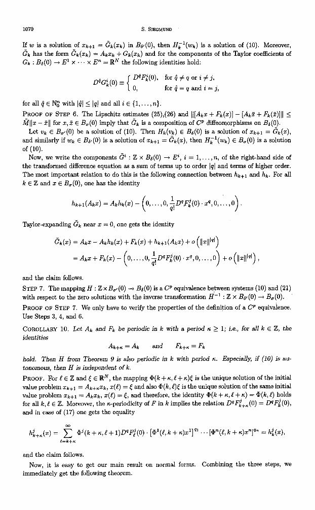
1070 S. SIEGMUND

If w is a solution of xk+r = Ck(xk) in Bat(O), then HL’( wk is a solution of (10). Moreover, ) Ck has the form Ck(xk) = &xk + Ck(xk) and for the components of the Taylor coefficients of Gk :&(o) + t? X ..* x E” = RN the following identities hold:

D”G;(O) z D@FL(O), for i # q or i # j, o

, for i = q and i = j,

for all G E NJ;; with ]G] I IqJ and all i E (1,. . . ,n}.

PROOF OF STEP 6. The Lipschitz estimates (25),(26) and ]([&a: + Fk(X)] - [i&Z + 4(x)]]] 5 A?]]x - z]] for x, 1 E B,(O) imply that Ck is a composition of 0’ diffeomorphisms on B&(O).

Let Vk E B,,(O) be a solution of (10). Then Hk(Vk) E &(O) is a dUtiOn of Xk+l = tik(X),

and similarly if wk E &r(O) is a solution of xk+l = Ck(x), then &‘(wk) E B,(O) is a solution of (10).

Now, we write the components ti : Z x B&(O) + E”, i = 1 , . . . , n, of the right-hand side of the transformed difference equation as a sum of terms up to order IqI and terms of higher order. The most important relation to do this is the following connection between hk+r and hk. For all k E Z and x E B,(O), one has the identity

hk+l(AkX) = A&r,(X) - . Xq, 0,. . . ,o .

Taylor-expanding Ck near x = 0, one gets the identity

ek(2) = Akx - hchc(Z) + Fk(x) + &+1(&X) + 0 (11X1[“‘)

=&X+&(X)- (

0 ,..., o+‘F~(o)*Xq,o ,..., 0 > (

+0 ~~X~~lql),

and the claim follows.

STEP 7. The mapping H : Z x B,, (0) --f Ba(O) is a 0’ equivalence between systems (10) and (21) with respect to the zero solutions with the inverse transformation H-l : Z x B&l (0) + B,(O).

PROOF OF STEP 7. We only have to verify the properties of the definition of a 0’ equivalence. Use Steps 3, 4, and 6.

COROLLARY 10. Let Ak and 4 be periodic in k with a period K 2 1; i.e., for all k E iz, the identities

Ak+n = A,, and Fk+n = Ftc

hold. Then H from Theorem 9 is abo periodic in k with period IE. Especially if (10) is au- tonomous, then H is independent of k.

PROOF. For e E Z and E E RN, the mapping @(k + K, I + K)< is the unique solution of the initial value problem Xk+l = &+nxk, x(e) = [ and also Q(k, a)[ is the unique solution of the same initial value problem xk+r = Akxk, x(e) = E, and therefore, the identity 9(k + K, c + K) = @(k, e) holds for all k,C E Z. Moreover, the n-periodicity of F in k implies the relation D’JFi+,(O) = DqFi(O), and in case of (17) one gets the equality

h;+,(x) = 2 @(k + ~,e + l)D”Fi(O) . [a’(!, k + IE)x~]‘~ . . . [a”(& k -t +?]” = h;(x), e=k+n

and the claim follows.

Now, it is easy to get our main result on normal forms. Combining the three steps, we immediately get the following theorem.

Nonautonomous Difference Equations 1071

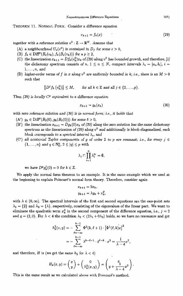
THEOREM 11. NORMAL FORM. Consider a difference equation

x/c+1 = h(x) . (29)

together with a reference solution v” : Z + RN. Assume that

(A) a neighbourhood UE(vo) is contained in Df for some E > 0, (B) d E DiffP(&(vk), fk(&(vk))) for a P 12, (C) the linearization xk+l = Dfk(v$k of (29) along v” has bounded growth, and therefore, [I]

the dichotomy spectrum consists of n, 1 5 n 2 N, compact intervals Xi = [ai, bi], i = 1 T”‘, n, and

(D) higher-order terms off in x along v” are uniformly bounded in k; i.e., there is an M > 0 such that

for all k E Z and all j E (2,. . . ,p}.

Then (29) is locally CP equivalent to a difference equation

with zero reference solution and (30) is in normal form; i.e., it holds that

(A’) P’)

((3

gk E Diffp(Ba(0),gk(&(O))) for some 6 > 0, the linearization Xk+l = Dgk(O)xk of (30) along the zero solution has the same dichotomy spectrum as the linearization of (29) ! a on g v” and additionally is block-diagonalized, each block corresponds to a spectral interval Xi, and all nontrivial Taylor components of g of order 2 to p are resonant; i.e., for every j E

(1,. * * I n} and q E N$, 2 < 141 5 p with

x,“iljXP’=0, i=l

we have Dqgi(O) = 0 fork E Z.

We apply the normal form theorem to an example. It is the same example which we used at the beginning to explain PoincarB’s normal form theory. Therefore, consider again

xk+l = 2xk,

Yk+l = h/k + xc:,

with X E (0, m). The spectral intervals of the first and second equations are the one-point sets X1 = (2) and X2 = {X}, respectively, consisting of the eigenvalues of the linear part. We want to eliminate the quadratic term xi in the second component of the difference equation, i.e., j = 2 and q = (2,O). For X < 4 the condition X2 < (2X1+ 0x2) holds, so we have no resonance and get

k-l

h;(x,y) = - c @(k,l+ 1). [@I@, kjx12 e=-oo

k-l

=- c ~“4-1 . 4t-k. x2 _ 1 &2

e=-oo A-4 ’

and therefore, H is (we get the same h2 for X < 4)

Hk(2,y)= (;.)+(h:(:,y)) = (y+&x+ This is the same result as we calculated above with Poincark’s method.

1072 S. SIEGMUND

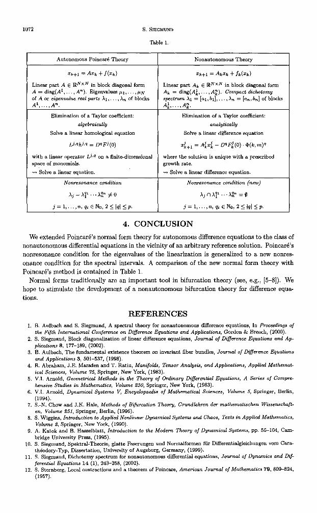
Table 1.

Autonomous Poincar6 Theory Nonautonomous Theory

lk+l = A% + fbk) “k+l = AkXk + fkbk)

Linear part A E RN x N in block diagonal form Linear part Ak E RN x N in block diagonal form A = diag(A’ , . , A”). Eigenvalues ~1,. . . , PN & = diag(A:, . . . , A;). Compact dichotomy of A or eigenvalue real parts Xl, . . , X, of blocks spectrum X1 = [al, bl], . . . , X, = [a,, bn] of blocks A’,...,A”. A;,...,A;.

Elimination of a Taylor coefficient: Elimination of a Taylor coefficient:

algebraically analytically

Solve a linear homological equation Solve a linear difference equation

Lj,4/& = DqFj (0) xi,, = A;xjk - DqF;(O) +(k,m)q

with a linear operator Ljlq on a finite-dimensional where the solution is unique with a prescribed space of monomials. growth rate.

+-+ Solve a linear equation. u) Solve a linear difference equation.

Nonresonance condition Nonresonance condition (new)

xj - $1 xff # 0 xj n $1 . A$= = 0

j = 1,. . . , It, Qi E No, 2 I IPI I P. j=l,...,n,qiEW0,2I{ql<p.

4. CONCLUSION

We extended Poincark’s normal form theory for autonomous difference equations to the class of nonautonomous differential equations in the vicinity of an arbitrary reference solution. Poincark’s nonresonance condition for the eigenvalues of the linearization is generalized to a new nonres- onance condition for the spectral intervals. A comparison of the new normal form theory with PoincarB’s method is contained in Table 1.

Normal forms traditionally are an important tool in bifurcation theory (see, e.g., [5-81). We hope to stimulate the development of a nonautonomous bifurcation theory for difference equa- tions.

REFERENCES 1. B. Aulbach and S. Siegmund, A spectral theory for nonautonomous difference equations, In Proceedings of

the Fifth International Conference on Difference Equations and Applications, Gordon & Breach, (2000). 2. S. Siegmund, Block diagonaliaation of linear difference equations, Journal of Difierence Equations and Ap-

plications 8, 177-189, (2002). 3. B. Aulbach, The fundamental existence theorem on invariant fiber bundles, Journal of Diflerence Equations

and Applications 3, 501-537, (1998). 4. R. Abraham, J.E. Marsden and T. Ratiu, Manifolds, Tensor Analysis, and Applications, Applied Mathemat-

ical Sciences, Volume 75, Springer, New York, (1983). 5. V.I. Arnold, Geometrical Methods in the Theory of Ordinary Differential Equations, A Series of Compre-

hensive Studies in Mathematics, Volume 250, Springer, New York, (1983). 6. V.I. Arnold, Dynamical Systems V, Encyclopaedia of Mathematical Sciences, Volume 5, Springer, Berlin,

(1994). 7. S.-N. Chow and J.K. Hale, Methods of Bifurcation Theory, Grundlehren der mathematischen Wissenschaft-

en, Volume 251, Springer, Berlin, (1996). 8. S. Wiggins, Introduction to Applied Nonlinear Dynamical Systems and Chaos, Texts in Applied Mathematics,

Volume 2, Springer, New York, (1990). 9. A. Katok and B. Hasselblatt, Introduction to the Modern Theory of Dynamical Systems, pp. 56-104, Cam-

bridge University Press, (1995). 10. S. Siegmund, Spektral-Theorie, glatte Fsserungen und Normalformen fiir Differentialgleichungen vom Cara-

th&dory-Typ, Dissertation, University of Augsburg, Germany, (1999). 11. S. Siegmund, Dichotomy spectrum for nonautonomous differential equations, Journal of Dynamics and Dif-

ferential Equations 14 (l), 243-258, (2002). 12. S. Sternberg, Local contractions and a theorem of Poincare, American Journal of Mathematics 79, 809-824,

(1957).

Nonautonomous Difference Equations 1073

13. S. Sternberg, On the structure of local homeomorphisms of Euclidian n-space. II., American Journal of MaULematics 80, 623-631, (1958).

14. S. Sternberg, The structure of local homeomorphisms. III, American Jounal of Mathematics 81, 578-604, (1959).

15. F. Takens, Partially hyperbolic fixed points, Topology 10, 133-147, (1971).