Embed Size (px)
Citation preview

NSOFT
Maxwell® 2D
Getting StartedA 2D Transient Linear Motion
Problem
December 2000

ii
NoticeThe information contained in this document is subject to changewithout notice.Ansoft makes no warranty of any kind with regard to this material,including, but not limited to, the implied warranties ofmerchantability and fitness for a particular purpose. Ansoft shall notbe liable for errors contained herein or for incidental or consequentialdamages in connection with the furnishing, performance or use ofthis material.This document contains proprietary information which is protectedby copyright. All rights are reserved.
Ansoft CorporationFour Station SquareSuite 200Pittsburgh, PA 15219(412) 261 - 3200
Motif is a trademark of the Open Software FoundationUNIX is a registered trademark of UNIX Systems Laboratories, Inc.WindowsTM and Windows NTTM are trademarks of Microsoft®
CorporationAIXwindowsTM is a trademark of International Business MachinesCorporationDECwindowsTM is a trademark of Digital Equipment CorporationOpenWindowsTM is a trademark of Sun Microsystems, Inc.
© Copyright 1994-2000 Ansoft Corporation

iii
Printing HistoryNew editions of this manual will incorporate all material updatedsince the previous edition. The manual printing date, which indicatesthe manual’s current edition, changes when a new edition is printed.Minor corrections and updates which are incorporated at reprint donot cause the date to change.Update packages may be issued between editions and containadditional and/or replacement pages to be merged into the manualby the user. Note that pages which are rearranged due to changes ona previous page are not considered to be revised.
Edition DateSoftwareRevision
1 October 1999 7.0
2 December 2000 8.0

iv
Welcome!This manual is a tutorial guide for setting up an electrostatic problemusing version 8.0 of Maxwell 2D, a software package for analyzingelectromagnetic fields in cross sections of structures.
Installation GuideWhen installing Maxwell 2D, refer to the Maxwell Installation Guide.
User’s ReferenceFor information on all of the Maxwell Control Panel and Maxwell 2DField Simulator commands, refer to the following sources:■ Maxwell Control Panel online documentation. This online
manual contains a detailed description of all of thecommands in the Maxwell Control Panel and in the Utilitiespanel. The Maxwell Control Panel allows you to create andopen projects, print screens, and translate files. Through theMaxwell Control Panel, you may access the Utilities panel,which allows you to either view licensing information (onthe workstation) or enter codewords (on the PC), adjustcolors, open and create 2D models, open and create plotsusing parametric equations, and evaluate mathematicalexpressions.
■ Maxwell 2D online documentation. This online manual containsa detailed description of Maxwell 2D and ParametricAnalysis module. The Parametric Analysis module allowsyou to define variables for different parts of the model, suchas geometric dimensions, material properties, andexcitations, so that you can assign different values to thesevariables during the solution. You then can analyze themodel’s behavior after these particular aspects of the modelare changed.

v
Getting StartedIf you are using Maxwell 2D for the first time, refer to the followingguides:■ Getting Started: An Electrostatic Problem■ Getting Started: A Magnetostatic Problem■ Getting Started: A 2D Parametric Problem
These short tutorials guide you through the process of setting up andsolving simple problems in Maxwell 2D. Using them will provideyou with a good overview of how to use the software.

vi
Using this ManualThis manual is organized in a manner that follows the sequence inwhich a problem is set up and solved as closely as possible. It isdivided into the following major sections:
For an overview of the general procedure to follow when you set up,solve, and analyze a problem, see Chapter 1, “Introduction.”
Section Title Contents
Chapter 1 Introduction Describes the purpose of Maxwell 2Dand summarizes the general procedurefor creating a model and solving aproblem.
Chapter 2 Creating theTransientProject
Describes the procedure for creating anew project directory and a Maxwell2D project.
Chapter 3 Accessing theSoftware
Describes how to open and run Max-well 2D. Also provides a brief overviewof the Maxwell 2D Executive com-mands window.
Chapter 4 Creating theModel
Describes the 2D Modeler and the pro-cedure for drawing the microstripmodel.
Chapter 5 DefiningMaterialsand Sources
Describes the procedure for assigningmaterials to the objects and definingboundary conditions and sources.
Chapter 6 Generating aSolution
Describes the procedure for enteringsolution criteria and generating a solu-tion.
Chapter 7 Analyzingthe Solution
Describes the procedure for analyzingthe results by plotting equipotentialcontours and calculating capacitance.
Index The index for the manual.

vii
Typeface ConventionsComputer Computer type is used for on-screen prompts
and messages, for field names, and for key-board entries that must be typed in theirentirety exactly as shown. For example, theinstruction “copy file1” means to type the wordcopy, to type a space, and then to type file1.
Menu/Command Computer type is also used to display the com-mands that are needed to perform a specifictask. Menu levels are separated by forwardslashes (/). For example, the instruction“Choose File/Open” means to choose the Opencommand under the File menu.
Italics Italic type is used for emphasis and for thetitles of manuals and other publications. Italictype is also used for keyboard entries when aname or a variable must be typed in place ofthe words in italics. For example, the instruc-tion “copy filename” means to type the wordcopy, to type a space, and then to type thename of a file, such as file1.
Keys Helvetica type is used for labeled keys on thecomputer keyboard. For example, the instruc-tion “Press Return” means to press the key onthe computer that is labeled Return.

viii

Contents-1
Table of Contents
1. Introduction . . . . . . . . . . . . . . . . . . . . . . . . . . . . . . . . . . 1-1Sample Problem . . . . . . . . . . . . . . . . . . . . . . . . . . . . . . . . . . . . . . . . . . . . . 1-3Results to Expect . . . . . . . . . . . . . . . . . . . . . . . . . . . . . . . . . . . . . . . . . . . . 1-3
2. Creating the Transient Project . . . . . . . . . . . . . . . . . . . 2-1Access the Maxwell Control Panel . . . . . . . . . . . . . . . . . . . . . . . . . . . . . . 2-2Create a Project Directory . . . . . . . . . . . . . . . . . . . . . . . . . . . . . . . . . . . . . 2-3
Add the Project Directory . . . . . . . . . . . . . . . . . . . . . . . . . . . . . . . . . . . . 2-4Create a Project . . . . . . . . . . . . . . . . . . . . . . . . . . . . . . . . . . . . . . . . . . . . . 2-5
Access the Project Directory . . . . . . . . . . . . . . . . . . . . . . . . . . . . . . . . . . 2-5Create the New Project . . . . . . . . . . . . . . . . . . . . . . . . . . . . . . . . . . . . . . 2-5Save Project Notes . . . . . . . . . . . . . . . . . . . . . . . . . . . . . . . . . . . . . . . . . . 2-6
3. Accessing the Software . . . . . . . . . . . . . . . . . . . . . . . . 3-1Open the New Project and Run the Software . . . . . . . . . . . . . . . . . . . . . . 3-2Executive Commands Window . . . . . . . . . . . . . . . . . . . . . . . . . . . . . . . . . 3-3
Executive Commands Menu . . . . . . . . . . . . . . . . . . . . . . . . . . . . . . . . . . 3-3Display Area . . . . . . . . . . . . . . . . . . . . . . . . . . . . . . . . . . . . . . . . . . . . . . 3-3Solution Monitoring Area . . . . . . . . . . . . . . . . . . . . . . . . . . . . . . . . . . . . 3-3
Sample Problem . . . . . . . . . . . . . . . . . . . . . . . . . . . . . . . . . . . . . . . . . . . . . 3-4General Procedure . . . . . . . . . . . . . . . . . . . . . . . . . . . . . . . . . . . . . . . . . . . 3-5
4. Creating the Model . . . . . . . . . . . . . . . . . . . . . . . . . . . . 4-1Specify Solver Type . . . . . . . . . . . . . . . . . . . . . . . . . . . . . . . . . . . . . . . . . . 4-2Specify Drawing Plane . . . . . . . . . . . . . . . . . . . . . . . . . . . . . . . . . . . . . . . 4-2

Contents-2
Access the 2D Modeler . . . . . . . . . . . . . . . . . . . . . . . . . . . . . . . . . . . . . . . 4-3Layout of the 2D Modeler . . . . . . . . . . . . . . . . . . . . . . . . . . . . . . . . . . . . . 4-4
General Areas . . . . . . . . . . . . . . . . . . . . . . . . . . . . . . . . . . . . . . . . . . . . . . 4-4Accessing Commands . . . . . . . . . . . . . . . . . . . . . . . . . . . . . . . . . . . . . . . 4-4Project Windows . . . . . . . . . . . . . . . . . . . . . . . . . . . . . . . . . . . . . . . . . . . 4-5Subwindows . . . . . . . . . . . . . . . . . . . . . . . . . . . . . . . . . . . . . . . . . . . . . . . 4-5
Set Up the Drawing Region . . . . . . . . . . . . . . . . . . . . . . . . . . . . . . . . . . . . 4-6Define the Drawing Size . . . . . . . . . . . . . . . . . . . . . . . . . . . . . . . . . . . . . 4-6
Create the Geometry . . . . . . . . . . . . . . . . . . . . . . . . . . . . . . . . . . . . . . . . . 4-7Keyboard Entry . . . . . . . . . . . . . . . . . . . . . . . . . . . . . . . . . . . . . . . . . . . . 4-7Drawing the Band Object . . . . . . . . . . . . . . . . . . . . . . . . . . . . . . . . . . . . . 4-8
Create a Rectangle . . . . . . . . . . . . . . . . . . . . . . . . . . . . . . . . . . . . . . . . . . . . 4-8Define the Band’s Name and Color . . . . . . . . . . . . . . . . . . . . . . . . . . . . . . . 4-8
Draw the Magnet . . . . . . . . . . . . . . . . . . . . . . . . . . . . . . . . . . . . . . . . . . . 4-9Draw the Left Bar . . . . . . . . . . . . . . . . . . . . . . . . . . . . . . . . . . . . . . . . . . 4-10Draw the Right Bar . . . . . . . . . . . . . . . . . . . . . . . . . . . . . . . . . . . . . . . . . 4-11
Select and Copy the Left Bar . . . . . . . . . . . . . . . . . . . . . . . . . . . . . . . . . . . . 4-11Rename the Right Bar . . . . . . . . . . . . . . . . . . . . . . . . . . . . . . . . . . . . . . . . . 4-12Displaying Zoomed Models . . . . . . . . . . . . . . . . . . . . . . . . . . . . . . . . . . . . . 4-12
Completed Geometry . . . . . . . . . . . . . . . . . . . . . . . . . . . . . . . . . . . . . . . . . 4-13Exit the 2D Modeler . . . . . . . . . . . . . . . . . . . . . . . . . . . . . . . . . . . . . . . . . . 4-13
5. Defining Materials and Boundaries . . . . . . . . . . . . . . . 5-1Setup Materials . . . . . . . . . . . . . . . . . . . . . . . . . . . . . . . . . . . . . . . . . . . . . 5-2
Access the Material Manager . . . . . . . . . . . . . . . . . . . . . . . . . . . . . . . . . . 5-3Material Manager Layout . . . . . . . . . . . . . . . . . . . . . . . . . . . . . . . . . . . . . 5-3
Objects . . . . . . . . . . . . . . . . . . . . . . . . . . . . . . . . . . . . . . . . . . . . . . . . . . . . . 5-3Materials . . . . . . . . . . . . . . . . . . . . . . . . . . . . . . . . . . . . . . . . . . . . . . . . . . . . 5-3Display Area . . . . . . . . . . . . . . . . . . . . . . . . . . . . . . . . . . . . . . . . . . . . . . . . . 5-4Material Attributes . . . . . . . . . . . . . . . . . . . . . . . . . . . . . . . . . . . . . . . . . . . . 5-4
Assign NdFe35 to the Magnet . . . . . . . . . . . . . . . . . . . . . . . . . . . . . . . . . 5-4Assign Copper to the Flanking Magnets . . . . . . . . . . . . . . . . . . . . . . . . . 5-5Assign a Vacuum to the Band . . . . . . . . . . . . . . . . . . . . . . . . . . . . . . . . . 5-5Assigning Materials to the Background . . . . . . . . . . . . . . . . . . . . . . . . . . 5-6Exit the Material Manager . . . . . . . . . . . . . . . . . . . . . . . . . . . . . . . . . . . . 5-7
Setup Boundaries and Sources . . . . . . . . . . . . . . . . . . . . . . . . . . . . . . . . . . 5-8Display the Boundary Manager . . . . . . . . . . . . . . . . . . . . . . . . . . . . . . . . 5-9Boundary Manager Screen Layout . . . . . . . . . . . . . . . . . . . . . . . . . . . . . 5-9
Boundary . . . . . . . . . . . . . . . . . . . . . . . . . . . . . . . . . . . . . . . . . . . . . . . . . . . 5-9Display Area . . . . . . . . . . . . . . . . . . . . . . . . . . . . . . . . . . . . . . . . . . . . . . . . . 5-9Boundary/Source Information . . . . . . . . . . . . . . . . . . . . . . . . . . . . . . . . . . . 5-9
Contents-3
Types of Boundary Conditions and Sources . . . . . . . . . . . . . . . . . . . . . . 5-10Set Voltage on Copper Bars . . . . . . . . . . . . . . . . . . . . . . . . . . . . . . . . . . . 5-11
Select the Copper Bars . . . . . . . . . . . . . . . . . . . . . . . . . . . . . . . . . . . . . . . . . 5-11Define a Functional Voltage . . . . . . . . . . . . . . . . . . . . . . . . . . . . . . . . . . . . 5-11Assign a Voltage . . . . . . . . . . . . . . . . . . . . . . . . . . . . . . . . . . . . . . . . . . . . . 5-12Assign the Coil Value . . . . . . . . . . . . . . . . . . . . . . . . . . . . . . . . . . . . . . . . . 5-12
Balloon the Background . . . . . . . . . . . . . . . . . . . . . . . . . . . . . . . . . . . . . . 5-13Select the Background . . . . . . . . . . . . . . . . . . . . . . . . . . . . . . . . . . . . . . . . . 5-13Assign Balloon Boundary . . . . . . . . . . . . . . . . . . . . . . . . . . . . . . . . . . . . . . 5-13
Displaying, Modifying, and Deleting Boundaries and Sources . . . . . . . . 5-14Exit the Boundary Manager . . . . . . . . . . . . . . . . . . . . . . . . . . . . . . . . . . . 5-14
6. Generating a Solution . . . . . . . . . . . . . . . . . . . . . . . . . . 6-1Access the Setup Solution Menu . . . . . . . . . . . . . . . . . . . . . . . . . . . . . . . . 6-2Modify Solution Criteria . . . . . . . . . . . . . . . . . . . . . . . . . . . . . . . . . . . . . . 6-3
Manual Mesh . . . . . . . . . . . . . . . . . . . . . . . . . . . . . . . . . . . . . . . . . . . . . . 6-3Create the Mesh . . . . . . . . . . . . . . . . . . . . . . . . . . . . . . . . . . . . . . . . . . . . . . 6-4Exit the Meshmaker . . . . . . . . . . . . . . . . . . . . . . . . . . . . . . . . . . . . . . . . . . . 6-5
Solver Residual . . . . . . . . . . . . . . . . . . . . . . . . . . . . . . . . . . . . . . . . . . . . 6-5Solver Choice . . . . . . . . . . . . . . . . . . . . . . . . . . . . . . . . . . . . . . . . . . . . . . 6-5Transient Analysis . . . . . . . . . . . . . . . . . . . . . . . . . . . . . . . . . . . . . . . . . . 6-6Transient Solution Criteria . . . . . . . . . . . . . . . . . . . . . . . . . . . . . . . . . . . . 6-6Exit Setup Solution . . . . . . . . . . . . . . . . . . . . . . . . . . . . . . . . . . . . . . . . . 6-6
Define the Motion Attributes . . . . . . . . . . . . . . . . . . . . . . . . . . . . . . . . . . . 6-7Define the Band Object . . . . . . . . . . . . . . . . . . . . . . . . . . . . . . . . . . . . . . 6-7Define the Moving Object . . . . . . . . . . . . . . . . . . . . . . . . . . . . . . . . . . . . 6-8Define the Stationary Objects . . . . . . . . . . . . . . . . . . . . . . . . . . . . . . . . . 6-8Define the Mechanical Transient . . . . . . . . . . . . . . . . . . . . . . . . . . . . . . . 6-8
Define the Motion Variables . . . . . . . . . . . . . . . . . . . . . . . . . . . . . . . . . . . . 6-9Define the Spring Constant . . . . . . . . . . . . . . . . . . . . . . . . . . . . . . . . . . 6-9Define the Weight . . . . . . . . . . . . . . . . . . . . . . . . . . . . . . . . . . . . . . . . . 6-9Define the Restoring Force . . . . . . . . . . . . . . . . . . . . . . . . . . . . . . . . . . 6-9Define the Damping Coefficient . . . . . . . . . . . . . . . . . . . . . . . . . . . . . . 6-9Define the Forces Factor . . . . . . . . . . . . . . . . . . . . . . . . . . . . . . . . . . . . 6-10Define the Mechanical Transient . . . . . . . . . . . . . . . . . . . . . . . . . . . . . 6-10
Exit the Motion Setup Window . . . . . . . . . . . . . . . . . . . . . . . . . . . . . . . . 6-10Generate the Solution . . . . . . . . . . . . . . . . . . . . . . . . . . . . . . . . . . . . . . . . . 6-11Monitoring the Solution . . . . . . . . . . . . . . . . . . . . . . . . . . . . . . . . . . . . . . . 6-11Completing the Solution Process . . . . . . . . . . . . . . . . . . . . . . . . . . . . . . . . 6-12
Viewing Statistics . . . . . . . . . . . . . . . . . . . . . . . . . . . . . . . . . . . . . . . . . . 6-13Viewing the Results . . . . . . . . . . . . . . . . . . . . . . . . . . . . . . . . . . . . . . . . . . 6-14

Contents-4
View the Plots . . . . . . . . . . . . . . . . . . . . . . . . . . . . . . . . . . . . . . . . . . . . . 6-14
7. Analyzing the Solution . . . . . . . . . . . . . . . . . . . . . . . . . 7-1Post Process the 0.1-second Time Step . . . . . . . . . . . . . . . . . . . . . . . . . . . 7-2
Access the Post Processor . . . . . . . . . . . . . . . . . . . . . . . . . . . . . . . . . . . . 7-2Post Processor Screen Layout . . . . . . . . . . . . . . . . . . . . . . . . . . . . . . . . . 7-3
General Areas . . . . . . . . . . . . . . . . . . . . . . . . . . . . . . . . . . . . . . . . . . . . . . . . 7-3Executing Commands . . . . . . . . . . . . . . . . . . . . . . . . . . . . . . . . . . . . . . . . . 7-3Project Window . . . . . . . . . . . . . . . . . . . . . . . . . . . . . . . . . . . . . . . . . . . . . . 7-3Subwindows . . . . . . . . . . . . . . . . . . . . . . . . . . . . . . . . . . . . . . . . . . . . . . . . . 7-3
Plotting the 0.1-second Flux Density . . . . . . . . . . . . . . . . . . . . . . . . . . . . 7-4Calculators . . . . . . . . . . . . . . . . . . . . . . . . . . . . . . . . . . . . . . . . . . . . . . . . 7-6
Plane Calculator . . . . . . . . . . . . . . . . . . . . . . . . . . . . . . . . . . . . . . . . . . . . . . 7-6Line Calculator . . . . . . . . . . . . . . . . . . . . . . . . . . . . . . . . . . . . . . . . . . . . . . . 7-6Number Calculator . . . . . . . . . . . . . . . . . . . . . . . . . . . . . . . . . . . . . . . . . . . . 7-6
Calculate the Induced Current . . . . . . . . . . . . . . . . . . . . . . . . . . . . . . . . . 7-7Calculate and Plot the 0.1-second Induced Current . . . . . . . . . . . . . . . . . 7-8
Load and Compute J . . . . . . . . . . . . . . . . . . . . . . . . . . . . . . . . . . . . . . . . . . . 7-8Refresh the Screen . . . . . . . . . . . . . . . . . . . . . . . . . . . . . . . . . . . . . . . . . . . . 7-8Plot J . . . . . . . . . . . . . . . . . . . . . . . . . . . . . . . . . . . . . . . . . . . . . . . . . . . . . . . 7-9
Return to the Executive Commands Window . . . . . . . . . . . . . . . . . . . . . 7-10Post Process the 0.3-second Time Step . . . . . . . . . . . . . . . . . . . . . . . . . . . 7-11
Plotting the 0.3-second Flux . . . . . . . . . . . . . . . . . . . . . . . . . . . . . . . . . . 7-11Calculate and Plot the 0.3-second Induced Current . . . . . . . . . . . . . . . . . 7-12
Load and Compute J . . . . . . . . . . . . . . . . . . . . . . . . . . . . . . . . . . . . . . . . . . . 7-12Refresh the Screen . . . . . . . . . . . . . . . . . . . . . . . . . . . . . . . . . . . . . . . . . . . . 7-12Plot J . . . . . . . . . . . . . . . . . . . . . . . . . . . . . . . . . . . . . . . . . . . . . . . . . . . . . . . 7-13
Exit Maxwell 2D . . . . . . . . . . . . . . . . . . . . . . . . . . . . . . . . . . . . . . . . . . . . 7-14Exit the Maxwell Software . . . . . . . . . . . . . . . . . . . . . . . . . . . . . . . . . . . . 7-14

Introduction 1-1
1
Introduction
Maxwell 2D is an interactive software package that uses finite element analy-sis to solve two-dimensional electromagnetic problems. To analyze a prob-lem, you specify the appropriate geometry, material properties, andexcitations for a device or system of devices. The Maxwell software then doesthe following:● Creates the required finite element mesh, either automatically or from
user-defined seeding requirements.● Iteratively calculates the desired field solution and special quantities of
interest, including force, torque, inductance, capacitance, and power loss.● With EMpulse, simulates the transient, large motion of the system.● Allows you to analyze, manipulate, and display field solutions.
1-2 Introduction
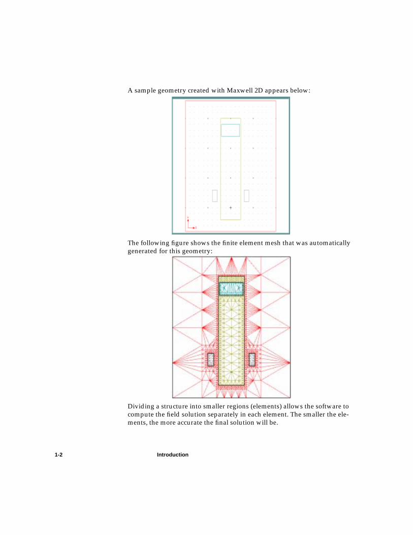
A sample geometry created with Maxwell 2D appears below:
The following figure shows the finite element mesh that was automaticallygenerated for this geometry:
Dividing a structure into smaller regions (elements) allows the software tocompute the field solution separately in each element. The smaller the ele-ments, the more accurate the final solution will be.

Sample Problem
Introduction 1-3
Sample ProblemIn this guide, you will draw, set up, and solve the transient motion simulationshown below:
This problem is a simple example of a time-dependent physics problem. Thesimulation incorporates the use of “mechanical components,” large motion,and a steady state source — in this case, a permanent magnet.
Results to ExpectAfter setting up the motion problem and generating a solution, you willobserve the following changes with respect to time:● The winding current.● The back EMF.● The flux linkage.● The position of the magnet.● The velocity of the magnet’s motion.
Time: This guide should take approximately 3 hours to work through.

Results to Expect
1-4 Introduction

Creating the Transient Project 2-1
2
Creating the Transient Project
This guide assumes that Maxwell 2D has already been installed as describedin the Maxwell Installation Guide.
Your goals in this chapter are as follows:● Create a project directory in which to save sample problems.● Create a new project in that directory in which to save the motion
problem.
➥Warning: If you have not installed the software or you are not set up to run the
software yet, STOP! Follow the instructions in the Maxwell InstallationGuide before proceeding with this guide.
Time: This chapter should take approximately 15 minutes to work through.

Access the Maxwell Control Panel
2-2 Creating the Transient Project
Access the Maxwell Control PanelTo access Maxwell 2D, you must first access the Maxwell Control Panel,which allows you to create and open projects for all Ansoft projects.
➤ To access the Maxwell Control Panel:● Do one of the following:
■ On a UNIX workstation, enter the following command at the UNIXprompt:
maxwell &
■ On the PC, double-click the left mouse button on the Maxwell icon.
The Maxwell Control Panel appears as shown below:
See the Maxwell Control Panel online documentation for a detailed descrip-tion of the other options in the Maxwell Control Panel. If the Maxwell ControlPanel doesn’t appear, refer to the Maxwell Installation Guide for possible rea-sons.You will create a new project directory to store the projects for the Maxwell2D Getting Started guides.

Create a Project Directory
Creating the Transient Project 2-3
Create a Project DirectoryThe first step in using Maxwell 2D to solve a problem is to create a projectdirectory and a project in which to save all the data associated with the prob-lem.A project directory is a directory that contains a specific set of projects createdwith the Ansoft software. You can use project directories to categorize projectsany number of ways. For example, you might want to store all projects relatedto a particular facility or application in one project directory.The Project Manager should still be on the screen. You will add the getstartdirectory that will contain the Maxwell 2D project you create using this Get-ting Started guide.
➤ Access the Project Manager and add the project directories:● Choose Projects from the Maxwell Control Panel. The Project Manager
appears as shown below, listing the current path and any existingprojects:
☞Note: If you’ve already created a project directory while working through one of
the other Getting Started guides, skip to the “Create a Project” section onpage 2-5.

Create a Project Directory
2-4 Creating the Transient Project
Add the Project Directory➤ Now add the project directory:
1. Choose Add from the Project Directories list at the bottom left of the win-dow. The following window appears, listing the directories and subdirec-tories:
2. Type the following in the Alias field:getst2d
3. Choose Make New Directory near the bottom of the pop-up window. Bydefault, getst2d appears in this field.
4. Choose OK.The directory getst2d is created under the current default project directory.You return to the Project Manager, and getst2d now appears in the ProjectDirectories list.
☞Note: Maxwell 2D projects are created in directories which have aliases — that
is, directories that have been identified as project directories using theAdd command.➤ Do the following if you want to temporarily change directories
for an alias:1. Choose Change Dir from the Project Directories box.2. Double-click the left mouse button on the desired directory.
(Choose ../ to move up a level in the directory structure.)3. After you are done, choose Cancel.
See the Maxwell Control Panel online documentation for more informa-tion on changing directories and other Project Manager functions.

Create a Project
Creating the Transient Project 2-5
Create a ProjectNow you are ready to create a new project named 2dmotion in the projectdirectory getst2d.
Access the Project DirectoryBefore you create the new project, access the project directory getst2d.
➤ Access the project directory:● Select getst2d from the Project Directories list at the bottom-left of the
menu. It is now highlighted.The current directory displayed at the top of the Project Manager menuchanges to show the path name of the directory associated with the aliasgetst2d. If you have previously created a model, it will be listed in the Projectsbox. Otherwise, the Projects box is empty — no projects have been created yetin this project directory.
Create the New Project➤ Create a new project as follows:
1. Choose New from the Projects area at the top-left of the menu. A windowsimilar to the following one appears:
2. Type 2dmotion in the Name field. Use the Back Space and Delete keys tocorrect typos.
3. If Maxwell 2D Version 8 does not appear in the Type field, do the follow-ing:a. Click the left mouse button on the software package listed in the Type
field. A menu appears, listing all of the Maxwell software packagesyou purchased.
b. Choose Maxwell 2D Version 8.4. Optionally, enter your name in the Created By field. The name of the per-
son who logged onto the system appears by default.5. Deselect Open project upon creation. This will allow you to enter project
notes prior to opening the project.6. Choose OK or press Return.

Create a Project
2-6 Creating the Transient Project
The information that you just entered is now displayed in the correspondingfields in the Project list. Because you created the project, Writable is selected,showing that you have access to the project.
Save Project NotesIt is a good idea to save notes about your new project so that the next timeyou use Maxwell 2D, you can view information about a project without open-ing it.
➤ Enter notes for the 2dmotion problem as follows:1. Leave Notes selected by default.2. Click the left mouse button in the area under the Notes option. This places
an I-beam cursor in the upper-left corner of the Notes area, indicating thatyou can begin typing text.
3. Enter your notes on the project, such as the following:This is the sample transient problem created usingthe Maxwell 2D and the 2D Linear Motion GettingStarted guide.
When you start entering project notes, the text of the Save Notes button(located below the Notes area) changes to black, indicating that it isenabled. Before you began typing in the Notes area, Save Notes wasgrayed out, or disabled.
4. When you are done entering the description, choose Save Notes to save it.After you do, the Save Notes option is grayed out again.
Now you are ready to open the new Maxwell 2D project and run Maxwell 2D.
☞Note: The Model option displays a picture of the selected model in the Notes
area. It is disabled now because you are creating a new project. After youcreate the 2dmotion problem, its geometry will appear in this area bydefault when the 2dmotion project is selected. For a detailed descriptionof the Model option, refer to the Maxwell Control Panel online documen-tation.
☞Note: Grayed out text on commands or buttons means that the command or
button is temporarily disabled.

Accessing the Software 3-1
3
Accessing the Software
In the last chapter, you created the getst2d project directory and created the2dmotion project within that directory.This chapter describes:● How to open the project you just created and run Maxwell 2D.● The Maxwell 2D Executive Commands window.● The general procedure for creating a linear motion problem in Maxwell
2D.● The sample problem and the procedures you will use to simulate its time-
varying magnetic fields.
Time: This chapter should take approximately 10 minutes to work through.

Open the New Project and Run the Software
3-2 Accessing the Software
Open the New Project and Run the SoftwareThe newly created 2dmotion project should still be highlighted in the Projectsbox. (If it is not, move the cursor on it and click the left mouse button.)
➤ Run Maxwell 2D as follows:● Choose Open from the Project Manager.The Executive Commands window of Maxwell 2D appears as shown below:
Depending on the licenses already installed for the software, your windowmay appear slightly different.

Executive Commands Window
Accessing the Software 3-3
Executive Commands WindowThe Executive Commands window is divided into three sections: the Execu-tive Commands menu, the display area, and the Solution Monitoring area.
Executive Commands MenuThe Executive Commands menu acts as a doorway to each step of creatingand solving the model problem. You select each module through the Execu-tive Commands menu, and the software brings you back to this menu whenyou are finished. You also view the solution process through this menu.
Display AreaThe display area shows the project’s geometry in a model window, or thesolutions to the problem once a solution has been generated. Since youhaven’t yet drawn the model, this area is blank. The commands along the bot-tom of the window allow you to change your view of the model:
The buttons along the top of the window are used when you are generatingand analyzing a solution. These are described in more detail in Chapter 6,“Generating a Solution.”
Solution Monitoring AreaThis area displays solution profile and convergence information while theproblem is solving, as described in Chapter 6, “Generating a Solution.”
Zoom In Zooms in on an area of the window, magnifying the view.Zoom Out Zooms out of an area, shrinking the view.Fit All Changes the view to display all items in the window. Items will
appear as large as possible without extending beyond the window.Fit Drawing Displays the entire drawing space.Fill Solids Displays objects as solids rather than outlined objects. Toggles
with Wire Frame.Wire Frame Displays objects as wire-frame outlines. Toggles with Fill Solids.

Sample Problem
3-4 Accessing the Software
Sample ProblemThe rest of this manual guides you through the setup, solution, and analysisof a simple linear motion problem. The sample problem, shown below, is amechanically coupled, time-dependent structure that includes the following:● A band object. Band objects define the region in which motion occurs. No
motion can ever take place outside the band object.● A magnet that moves linearly in the negative x-direction within the band
object.● Two copper bars that flank the band object and magnet as it moves.Detailed dimensions and instructions for drawing this model are given inChapter 4, “Creating the Model.”

General Procedure
Accessing the Software 3-5
General ProcedureThe general procedure for solving 2D linear motion problem is as follows:1. Use the Solver command to specify which of the following electric or
magnetic field quantities to compute:■ Electrostatic■ Magnetostatic■ Eddy Current■ DC Conduction■ AC Conduction■ Eddy Axial■ Transient■ Thermal
2. Use the Drawing command to select one of the following model types:
3. Use the Define Model command to access the following options:
4. Use the Setup Materials command to assign materials to all objects in thegeometric model.
5. Use the Setup Boundaries/Sources command to define the boundaries andsources for the problem.
6. Use the Setup Executive Parameters command to compute the following:■ Matrix (capacitance, inductance, admittance, impedance, or conduc-
tance matrix, depending on the selected solver)■ Force■ Torque■ Flux Linkage
☞Note: Only the Maxwell 2D packages that you have purchased and installed
appear on the menu.
XY Plane Visualize cartesian models as sweeping perpendicu-larly to the cross-section.
RZ Plane Visualize axisymmetric models as revolving around anaxis of symmetry in the cross-section.
Draw Model Allows you to access the 2D Modeler and draw theobjects that make up the geometric model.
Group Objects Allows you to group discrete objects that are actuallyone electrical object. For instance, two terminations of aconductor that are drawn as separate objects in thecross-section can be grouped to represent one conduc-tor.

General Procedure
3-6 Accessing the Software
■ Current Flow7. Use the Setup Solution/Options command to enter parameters that affect
how the solution is computed.8. Use the Setup Solution/Motion Setup command to define the motion
parameters of the system.9. Use the Solve/Nominal Problem command to solve for the appropriate
field quantities.10. Use the Post Process/Nominal Problem command to analyze the solution
as follows:■ Plot the field solution. Common quantities (such as φ, E, and D) are
directly accessible from menus and can be plotted a number of ways.For instance, you can display a plot of equipotential contours or youcan graph potential as a function of distance.
■ Use the calculators. A post processor allows you to take curls, diver-gences, integrals, and cross and dot products to derive special quanti-ties of interest.
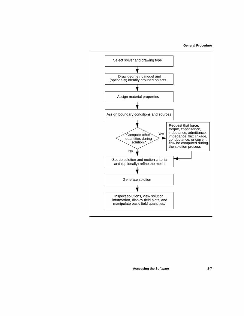
The commands shown in the Executive Commands menu must be chosen inthe sequence in which they appear. For example, you must first create a geo-metric model with the Define Model command before you specify materialcharacteristics for objects with the Setup Materials command. A checkmarkappears on the menu next to the completed steps.These steps are summarized in the following flowchart:
General Procedure
Accessing the Software 3-7
Select solver and drawing type
Draw geometric model and
Assign material properties
Assign boundary conditions and sources
Yes
No
Request that force,
Set up solution and motion criteria
Generate solution
Inspect solutions, view solution
Compute otherquantities during
solution?
torque, capacitance,inductance, admittance,impedance, flux linkage,
flow be computed duringthe solution process
and (optionally) refine the mesh
information, display field plots, and manipulate basic field quantities.
(optionally) identify grouped objects
conductance, or current

General Procedure
3-8 Accessing the Software

Creating the Model 4-1
4
Creating the Model
In the last chapter, you opened the 2dmotion project, examined the ExecutiveCommands window, and reviewed the procedure for creating a 2D model.Now you are ready to use Maxwell 2D and EMpulse to solve the linearmotion problem. The first step is to create the geometry for the system beingstudied.This chapter shows you how to create the geometry for the motion problemthat was described in Chapter 1, “Introduction,” and in Chapter 3, “Accessingthe Software.”Your goals for this chapter are as follows:● Set up the problem region.● Create the objects that make up the geometric model.● Save the geometric model to a disk file.
Time: The total time needed to complete this chapter is approximately 35 min-utes.

Specify Solver Type
4-2 Creating the Model
Specify Solver TypeThe Maxwell 2D Executive Commands window should still be on the screen.Before you start drawing your model, you need to specify which field quanti-ties to compute. By default, Electrostatic appears as the Solver type. Becauseyou will be solving a motion problem, you will need to select it as the solvertype.
➤ Select the solver type:● Choose Transient from the Solver menu.
Specify Drawing PlaneThe model you will be drawing is actually the xy cross-section of a structurethat extends into the z direction. This is known as a cartesian or xy planemodel. By default, XY Plane appears as the Drawing plane. Because the modelyou will be creating is in the xy plane, leave this type selected.Now you are ready to draw the model.

Access the 2D Modeler
Creating the Model 4-3
Access the 2D ModelerTo draw the geometric model, use the 2D Modeler, which allows you to createtwo-dimensional structures.
➤ Access the 2D Modeler:● Choose Define Model/Draw Model. The 2D Modeler appears as shown
below:
☞Note: Throughout this manual, “choose” means to move the cursor to the
appropriate field or menu item and click any mouse button. Also,sequences of commands will be presented as Menu/Command. Forexample, “choose Model/Drawing Units” means to display the Modelmenu and then click on the Drawing Units command.

Layout of the 2D Modeler
4-4 Creating the Model
Layout of the 2D ModelerThe following sections provide a brief overview of the 2D Modeler.
General AreasThe 2D Modeler is divided into the following general areas:
For more information on these areas of the 2D Modeler, refer to the Maxwell2D online documentation.
Accessing CommandsYou can use either the tool bar to access the most commonly used commands,or the menu bar to access any of the commands in the 2D Modeler.
➤ To access commands from the menu, do one of the following:● Use the mouse buttons in the following ways:
■ Use the left mouse button to access, execute, and complete com-mands.
■ Use the right mouse button to abort commands.
Menu Bar Appears at the top of the 2D Modeler window. Each itemin the menu bar has a menu of commands associated withit.
Tool Bar Appears below the menu bar in the 2D Modeler windowas either a vertical stack or horizontal row of icons. Theicons give you easy access to the most frequently usedcommands.
Drawing Region Appears as the grid-covered area in which you drawobjects.
Message Bar Appears at the bottom of the screen. It displays the nameof that part of the software program and its version num-ber, help messages for commands, mouse button func-tions, number of items currently selected, andmagnification level when you change the view in a sub-window.
Status Bar Appears below the message bar. It contains fields that dis-play the coordinates of the mouse and which allow you toenter coordinates for object point. It also displays the cur-rent unit of length and the snap-to-point behavior of themouse.

Layout of the 2D Modeler
Creating the Model 4-5
● Use the keyboard in the following ways:■ Use the Alt key to display the commands for a menu.
■ Use the hotkeys, which appear next to the names of the commands inthe menus, to access a command.
■ Use the arrow or Tab keys to move around in the menu.
Project WindowsThe outermost window in the 2D Modeler is called the project window. Aproject window contains the geometry for a specific project and displays theproject’s name in its title bar. By default, one subwindow is contained withinthe project window.
SubwindowsSubwindows, or view windows, contain the drawing region in which youdraw the geometric model. By default, this window:● Has points specified in relation to a local uv coordinate system: the u-axis
is horizontal; the v-axis is vertical, and the origin is marked by a cross inthe middle of the window.
● Uses millimeters as the default drawing unit.● Has grid points 2 millimeters apart. The default window size is 70 mm by
100 mm.
☞Note: If you do not have an Alt key on your keyboard, use any one of the fol-
lowing keys instead:● The Meta key.● The Extend char key.● The Compose key.In this manual, however, it will be referred to as the Alt key.
☞Note: Optionally, open additional projects in the 2D Modeler using the File/
Open command. Opening several projects at once is useful if you want tocopy objects between geometries. See the Maxwell 2D online documen-tation for more details.
☞Note: If a geometry is complex, you may want to open additional subwindows
so that you can alter your view of the geometry from one subwindow tothe next. To do so, use the Windows commands that are described in theMaxwell 2D online documentation. For the linear motion geometry,however, a single subwindow is sufficient.

Set Up the Drawing Region
4-6 Creating the Model
Set Up the Drawing RegionThe first step in using the 2D Modeler is to specify the drawing units to use increating the model.
➤ Set up the drawing region as follows:1. Choose Model/Drawing Units. The following window appears:
2. Select inches from the list.3. Select Rescale to new units if it is not already selected. This rescales the
current units (mm) to inches.4. Choose OK.The units are changed from millimeters to inches, and inches now appearsnext to UNITS in the status bar at the bottom of the modeling window.
Define the Drawing SizeWith the drawing region defined, you can now specify the drawing size. Thiswill allow you to more easily locate exact points in the model.
➤ Define the drawing size:1. Choose Model/Drawing Size. The Drawing Size window appears.2. Enter -5 for the X Minima value. Press the Tab key to move to the next
field.3. Enter -2 for the Y Minima value. Again, use the Tab key to move to the
next field.4. Enter 5 for the X Maxima value. Press the Tab key.5. Enter 9 for the Y Maxima value.6. Leave all other values set to their defaults.7. Choose OK. The drawing size is now defined and the window closes.You return to the 2D Modeler.

Create the Geometry
Creating the Model 4-7
Create the GeometryNow you are ready to draw the objects that make up the geometric model. Allobjects are created using the Object commands as described in the followingsections.
Keyboard EntryWhen you specified the drawing region, you changed the drawing units frommillimeters to inches and left the default grid spacing set to two inches. In thefollowing section, several of the points that you will select as you createobjects lie between grid points. You can position these points in one of twoways:● Change the grid spacing so that the object’s dimensions lie on grid points.● Use “keyboard entry” — that is, enter the coordinates directly into the U
and V fields in the status bar.If you change grid spacing, the screen may become cluttered with too manytightly-spaced grid points and make point selection difficult. Therefore, usekeyboard entry to enter several of the dimensions of the sample geometry.
☞Note: To change the grid spacing, use the Model/Grid command. To change the
size of the problem region, use the Model/Drawing Size command. Formore details on these commands, see the Maxwell 2D online documenta-tion.

Create the Geometry
4-8 Creating the Model
Drawing the Band ObjectThe band consists of a simple rectangle in which the magnet will fall.
Create a Rectangle
Create a rectangle to represent the substrate. Because the vertices of the bandobject do not lie on an exact axis point, use the keyboard to enter the points.
➤ Create the rectangle:1. Choose Object/Rectangle. Again, the cursor changes to crosshairs.2. Select the first corner of the substrate, the upper-left corner, as follows:
a. Double-click the left mouse button in the U field in the status bar.b. Enter -1.1. (Use the Back Space and Delete keys to correct typos.)c. Use the Tab key to move to the V field in the status bar.d. Enter 7.5.
3. Press Return or use the mouse to choose Enter. The dU and dV fieldappear, displaying the offset distances from the initial point. Because youhave not specified an offset, these fields are set to zero.
4. Select the second corner of the substrate:a. Double-click the left mouse button in the U field in the status bar.b. Enter 1.1.c. Use the Tab key to move to the V field in the status bar.d. Enter –1.
5. Press Return or choose Enter from the status bar to accept the point.After you do, the New Object window appears:
Define the Band’s Name and Color
By default, objects you create are assigned the name objectx and the color red,and the Name field is selected.
➤ Define the name and color as follows:1. Type band in the Name field. Do not press Return.2. Click the left mouse button on the red box. A palette of 16 colors appears.3. Click the left mouse button on one of the green boxes in the palette.4. Choose OK.
☞Note: Be sure to change the name of the object to indicate its function and to
assign a different color to different objects. This will be important laterwhen you assign boundary conditions, voltages, and so forth.
Create the Geometry
Creating the Model 4-9
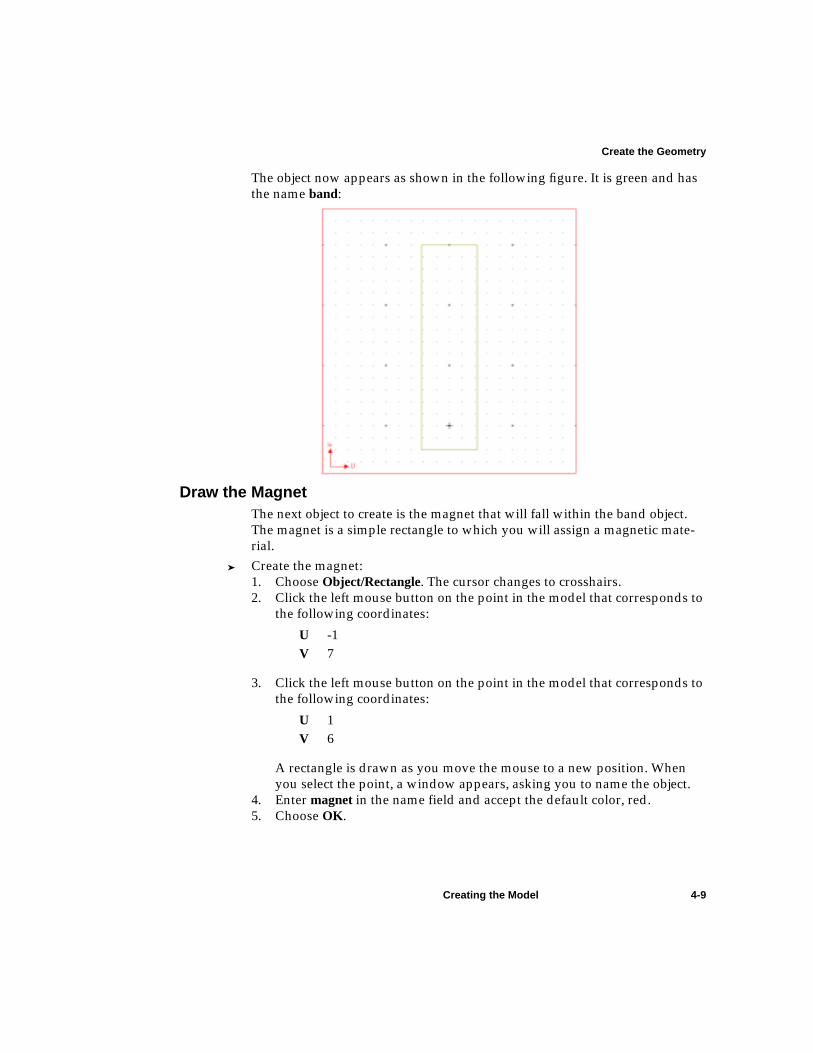
The object now appears as shown in the following figure. It is green and hasthe name band:
Draw the MagnetThe next object to create is the magnet that will fall within the band object.The magnet is a simple rectangle to which you will assign a magnetic mate-rial.
➤ Create the magnet:1. Choose Object/Rectangle. The cursor changes to crosshairs.2. Click the left mouse button on the point in the model that corresponds to
the following coordinates:
3. Click the left mouse button on the point in the model that corresponds tothe following coordinates:
A rectangle is drawn as you move the mouse to a new position. Whenyou select the point, a window appears, asking you to name the object.
4. Enter magnet in the name field and accept the default color, red.5. Choose OK.
U -1V 7
U 1V 6

Create the Geometry
4-10 Creating the Model
Draw the Left BarNow that you have drawn the band and the magnet, draw the left bar. Theleft and right bars are used to simulate the cross-sections of copper coils. Dur-ing the solution generation, the magnet’s change in position and time willcause a change in flux. The copper bars increase the flux, allowing you tomore easily observe this effect.
➤ Create the left bar:1. Choose Object/Rectangle. The cursor changes to crosshairs.2. Click the left mouse button on the point in the model that corresponds to
the following coordinates:
3. Click the left mouse button on the point in the model that corresponds tothe following coordinates:
A rectangle is drawn as you move the mouse to a new position. Whenyou select the point, a window appears, asking you to name the object.
4. Enter left in the name field.5. Change the color to grey.6. Choose OK.
U -2V 1.5
U -1.5V .5

Create the Geometry
Creating the Model 4-11
Draw the Right BarBecause the left and right microstrip have the same dimensions, create theright microstrip by copying the left one.
Select and Copy the Left Bar➤ Create the right bar:
1. Click the left mouse button on the left bar to select it as the object to becopied. A double outline appears around it, indicating that it has beenselected.
2. Choose Edit/Duplicate/Along Line. You must now select two points: firstan “anchor” point, and then a “target” point, which will be the new loca-tion for the anchor point.
3. Choose the lower-left corner of the left bar as the anchor point. After youdo, two new fields appear in the status bar: dU and dV. These fields allowyou to select the target point by specifying its offset from the anchor pointrather than its u- and v-coordinates.
4. Enter 3.5 in the field dU to specify the offset between the anchor and tar-get points.
5. Press Return or use the mouse to choose Enter. The Linear Duplicateswindow appears.
6. Leave the default 2 in the Total Number field.7. Choose OK to accept the value and complete the command.Now both bars have been created. By default, the new object — the right bar— is the selected object.
☞Note: As an alternative to selecting an object by clicking on it, use the Edit/
Select commands. After an object or objects are selected, they are theobjects on which all other Edit commands operate. See the Maxwell 2Donline documentation for more details on the Edit commands.

Create the Geometry
4-12 Creating the Model
Rename the Right Bar
The 2D Modeler automatically assigns names to copied objects by appendinga number to the end of the original object’s name. For instance, the right bar isassigned the name left1 because it is the first copy of the object left. Because itis a good idea to assign meaningful names to objects, change the name of left1to right.
➤ Rename the right bar:1. Choose Edit/Attributes/Rename. A window which lists the names of all
selected objects appears. Because left1 is the only selected object, itappears in the field beneath the object list.
2. Change the name left1 that appears below the list to right.3. Choose Rename. The new name now appears in the object list at the top of
the window.4. Choose OK.
Since you will create other objects, it is a good idea to deselect the right bar.➤ Deselect the right bar:
● Click the left mouse button on the right bar.The bar is deselected.
Displaying Zoomed Models
Scroll bars appear on the right side and bottom of the subwindow when theentire geometric model is not displayed in the window. In these cases, use thescroll bars to change your view.
➤ To change your view, do one of the following:● Click the left mouse button on the arrow buttons that appear at the top
and bottom of the scroll bar.● To scroll through the model:
1. Move the cursor to the off-colored bar, or “thumb scroll,” thatappears in the scroll bar.
2. Drag the thumb scroll up, down, left, or right in the scroll bar to theportion of the model that you want to display.
For instance, to pan down a geometric model, drag the thumb scroll in thevertical scroll bar down. If the portion of the geometry in which you are inter-ested does not appear, continue to manipulate the thumb scrolls until it does.

Completed Geometry
Creating the Model 4-13
Completed Geometry➤ Now fit all objects of the model in the window.
● Choose Window/Change View/Fit All. The completed geometry shouldnow resemble the following one:
Exit the 2D Modeler➤ Exit the 2D Modeler as follows:
1. Choose File/Exit. A window appears, prompting you to save the defaultwindow size.
2. Choose Yes to save the window settings. A second window appears,prompting you to save the changes before exiting. Because the Maxwell2D Modeler does not automatically save changes, you must either use theFile/Save command to save the changes, or save them as you exit themodule.
3. Choose Yes. The geometry is saved to a disk file in the project directory2dmotion.pjt and the Executive Commands window appears.
A checkmark appears next to Define Model, indicating that this step has beencompleted.
☞Note: Because none of the objects that you created are electrically connected at
any point in a three-dimensional rendering of the model, you do nothave to use the Define/Model/Group Objects command. For more detailson this command, refer to the Maxwell 2D online documentation.

Exit the 2D Modeler
4-14 Creating the Model

Defining Materials and Boundaries 5-1
5
Defining Materials and Boundaries
Now that you have drawn the geometry for the motion problem and returnedto the Executive Commands window, you are ready to set up the problem.Your goals for this chapter are as follows:● Assign materials to each object in the geometric model.● Define any boundary conditions, such as the behavior of the electric field
at the edge of the problem region and potentials on the surfaces of thebars.
Time: The total time needed to complete this chapter is approximately 35minutes.

Setup Materials
5-2 Defining Materials and Boundaries
Setup MaterialsTo define the material properties for the objects in the geometric model, youmust:● Assign the properties of NdFe35 to the magnet.● Assign copper to the bars.In general, to assign materials to objects:1. If necessary, add materials with the properties of the objects in your
model to the material database.2. Assign a material to each object in the geometric model:
a. Select the object(s) for which a specific material applies.b. Select the appropriate material.c. Choose Assign to assign the selected material to the selected object(s).
In this sample problem, you do not have to add materials to the material data-base — all materials that you will need are already included in the globalmaterial database that the simulator makes available to every project.
☞Note: You must assign a material to each object in the model.

Setup Materials
Defining Materials and Boundaries 5-3
Access the Material Manager➤ Access the Material Manager:
● Choose Setup Materials. The Material Manager appears:
Material Manager LayoutThe Material Manager (Material Setup window) is divided into several areasthat allow you to define and assign material properties.
Objects
The names of all the objects in the model appear in the Object list on the leftside of the menu along with their assigned materials. Only the object back-ground is assigned a material — vacuum — by default. UNASSIGNEDappears next to all other object names.
Materials
All materials in the global material database appear in the Material list on theleft side of the menu. External (Lock) appears next to each global material’sname, indicating that the properties of these objects cannot be changed. Mate-rials that you add to the database appear in the Material list with Local dis-played under Definition. Local materials may be modified.
☞Note: For the sample problem, you do not have to add any new materials to
the database. You will use the default materials contained within theglobal database. For details on how to create new materials, refer to theMaxwell 2D online documentation.

Setup Materials
5-4 Defining Materials and Boundaries
Display Area
The model is displayed so that you can choose objects simply by clicking onthem. The following buttons that appear at the bottom of the display areaallow you to manipulate your view of the model:
■ Zoom In■ Zoom Out■ Fit All■ Fit Drawing■ Fill Solids■ Window
They perform the same functions as the commands with the same names thatappear on the Model and Window menus of the 2D Modeler. These aredescribed in more detail in the Maxwell 2D online documentation.
Material Attributes
The Material Attributes area that appears below the geometric model displaysthe properties of the selected material. For instance, to display the attributesof glass, choose glass from the Material list on the left side of the menu.
Assign NdFe35 to the MagnetNow assign a material to the magnet.
➤ Assign a material to the magnet:1. Select magnet from the Object list or click on the substrate in the geomet-
ric model. Capitalized material names are listed first.2. Select NdFe35 from the Material list. If it does not appear in the box, use
the scroll bars to scroll through the list as described in Chapter 4, “Creat-ing the Model.”
3. Choose Assign. The Assignment Coord. Sys. window appears, allowingyou to define the alignment of the x-axis.
4. Select Align with a given direction. Because the magnet will move perpen-dicular to the x-axis, you will need to define the direction of motionaccordingly.
5. Enter 90 in the Angle field.6. Choose OK. The Assignment Coord. Sys. window closes.NdFe35 now appears next to magnet in the Object list.

Setup Materials
Defining Materials and Boundaries 5-5
Assign Copper to the Flanking MagnetsNow you can assign copper to the bars that flank the band.
➤ Assign materials to the conductors:1. Choose Multiple Select from the top of the menu, if it isn’t already
selected.2. Do one of the following to choose left and right from the object list:
■ If you are running the software on a workstation, click the left mousebutton on each of the object names.
■ If you are running the software on a PC, do one of the following:● Hold down the Ctrl key while clicking the left mouse button
on each of the object names.● Hold down the Shift key and click on the last object name.
To deselect an object, simply click the left mouse button on it, or for PCs,hit Ctrl-click to deselect a selected object.
3. Choose copper from the Material box.4. Choose the Assign button.The magnets have now been assigned the properties of a perfect conductor (agood approximation of which is copper). Also, copper appears next to thoseobjects’ names.
Assign a Vacuum to the BandNow assign a vacuum to the band object.
➤ Assign a material to the magnet:1. Select band from the Objects list or click on the substrate in the geometric
model. Capitalized material names are listed first.2. Select vacuum from the Material list, if it is not already selected. If it does
not appear in the box, use the scroll bars to scroll through the list asdescribed in Chapter 4, “Creating the Model.”
3. Choose Assign.Vacuum now appears next to band in the Object list.
☞Note: The potentials on the surfaces of conductors are specified with the Setup
Boundaries/Sources command that is described later in this chapter.

Setup Materials
5-6 Defining Materials and Boundaries
Assigning Materials to the BackgroundThe background object is the only object that is assigned a material by default.Include it as part of the problem region in which to generate the solution.When a material name — such as vacuum — appears next to background inthe Object list, the background object is included as part of the solutionregion.Because the model is assumed to be surrounded by a vacuum, accept thedefault material, vacuum, for the background.
☞Note: In some cases, such as when all objects and electromagetic fields of inter-
est are contained within an enclosure, including the background as partof the problem region wastes computing resources. It also prevents youfrom setting boundary conditions defining an external electric or mag-netic field for the model.➤ In these cases, exclude the background from the solution as
follows:1. Choose background from the Material list.2. Choose the Exclude button that appears above the Object
list. This button toggles between Include, the default, andExclude.
EXCLUDED then appears next to background in the Object list, indicat-ing that it will not be included as part of the solution region.However, do not exclude the background from the model.

Setup Materials
Defining Materials and Boundaries 5-7
Exit the Material ManagerNow materials have been assigned to each object.
➤ Exit the Material Setup window as follows:1. Choose Exit from the bottom-left of the Material Setup window. A win-
dow with the following prompt appears:Save changes before closing?
2. Choose Yes.You are returned to the Executive Commands menu. A checkmark nowappears next to Setup Materials, and Setup Boundaries/Sources is enabled.
☞Note: If you exit the Material Manager before excluding or assigning a mate-
rial to each object in the model, a checkmark does not appear next toSetup Materials on the Executive Commands menu, and Setup Bound-aries/Sources remains disabled.

Setup Boundaries and Sources
5-8 Defining Materials and Boundaries
Setup Boundaries and SourcesAfter setting material properties, the next step in creating the motion model isto define boundary conditions and sources.By default, the surfaces of all objects are Neumann or natural boundaries.That is, the magnetic field is defined to be perpendicular to the edges of theproblem space, and continuous across all object interfaces.To finish setting up the motion problem, you need to explicitly define the fol-lowing:● The voltages on the two copper bars.● The behavior of the electric field on all surfaces exposed to the area
beyond the problem region. Because you included the background aspart of the problem region, this exposed surface is that of the backgroundobject.
☞Note: Maxwell 2D will not solve the problem unless you specify some type of
source or magnetic field — either a current source, an external field sourceusing boundary conditions, or a permanent magnet. In this model, thecopper bars serve as sources of electric potential.
Setup Boundaries and Sources
Defining Materials and Boundaries 5-9
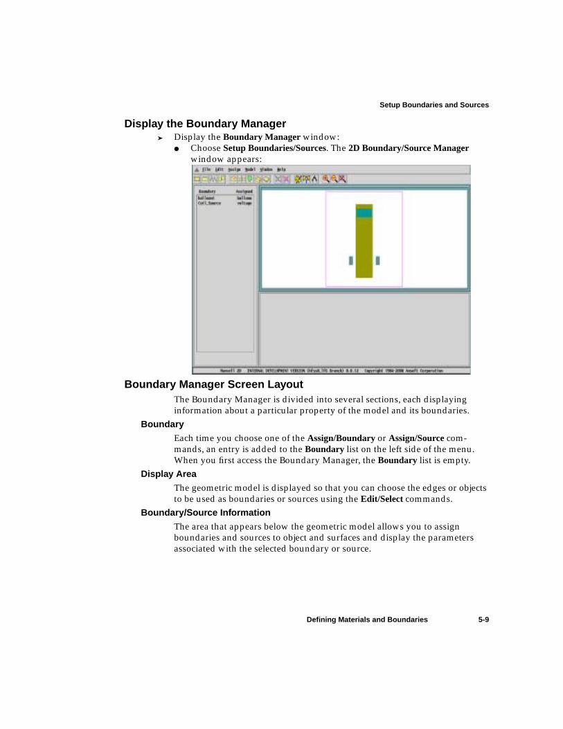
Display the Boundary Manager➤ Display the Boundary Manager window:
● Choose Setup Boundaries/Sources. The 2D Boundary/Source Managerwindow appears:
Boundary Manager Screen LayoutThe Boundary Manager is divided into several sections, each displayinginformation about a particular property of the model and its boundaries.
Boundary
Each time you choose one of the Assign/Boundary or Assign/Source com-mands, an entry is added to the Boundary list on the left side of the menu.When you first access the Boundary Manager, the Boundary list is empty.
Display Area
The geometric model is displayed so that you can choose the edges or objectsto be used as boundaries or sources using the Edit/Select commands.
Boundary/Source Information
The area that appears below the geometric model allows you to assignboundaries and sources to object and surfaces and display the parametersassociated with the selected boundary or source.

Setup Boundaries and Sources
5-10 Defining Materials and Boundaries
Types of Boundary Conditions and SourcesThere are two types of boundary conditions and sources that you will use inthis problem:
You will assign boundary conditions and sources to the following objects inthe geometry:
There are several ways to select objects’ surfaces, but in this sample problemyou will select each object individually. As a result, the object’s surface will beselected.
Balloon boundary Can only be applied to the outer boundary and models inwhich the structure is infinitely far away from all otherelectromagnetic sources.
Voltage sources Specifies the voltage on an object in the model. The elec-tric scalar potential, φ, is set to a constant value, forcingthe electric field to be perpendicular to the objects’ sur-faces.
Left bar This surface will be assigned a stranded voltage of 0volts.
Right bar This surface will be assigned a stranded voltage of 0volts.
Background The outer boundary of the problem region. This surfacewill be ballooned to simulate a magnetically insulatedsystem.

Setup Boundaries and Sources
Defining Materials and Boundaries 5-11
Set Voltage on Copper BarsTo define the voltage on the copper bars, you must first select them. Once anobject has been selected, it can be assigned either a source or boundary condi-tion. In this case, the copper bars will receive a voltage source.
Select the Copper Bars
Now, select the bars to which to assign the voltage.➤ Select the bars:
1. Choose Edit/Select/Object/By Clicking. The menu bar commands are dis-abled and the system expects you to select an item by clicking on it in themodel.
2. Click the left mouse button on the left and right bars. After you do, theybecome highlighted.
3. Click the right mouse button anywhere in the display area to stop select-ing objects.
Define a Functional Voltage
The copper bars possess a functional voltage based on the motion of the mag-net. To specify the source on the bars, you must first define the functionalvalue assigned to them.
➤ Define the functional voltage:1. Choose Assign/Source/Solid. The name source1 appears in the Boundary
list, and NEW appears next to it, indicating that it has not yet beenassigned to an object or surface.
2. Choose Options. The Property Options window appears.3. Select Function to define the source as a functional value.4. Choose OK. The Property Options window closes.5. Choose Functions. The Boundary/Source Symbol Table appears.6. Enter Coil in the blank field to the left of the equals sign.7. Enter 0 in the blank field to the right of the equals sign.8. Choose Add. Coil is added to the symbol table and is assigned a base
value of 0.9. Choose Done.The symbol table closes. You return to the 2D Boundary Manager.
☞Note: ➤ If the appropriate object is not highlighted, or if more than one
object is highlighted, do the following:1. Exit the select mode by cancelling the command or clicking
on the right mouse button.2. Choose Edit/Deselect All. After you do, no objects are
highlighted.3. Choose Edit/Select/Object/By Clicking and select the object.

Setup Boundaries and Sources
5-12 Defining Materials and Boundaries
Assign a Voltage
The voltage assigned to the copper bars is a functional value.➤ Assign the voltage to the bars:
1. Enter Coil_Source in the Name field2. Select Voltage to define the source as a voltage.3. Select Strand. The Winding button becomes active.4. Choose Winding to define a winding for the system. The following win-
dow appears:
5. Select left from the Object list.6. Leave Positive selected.7. Choose Assign.8. Select right from the Object list.9. Select Negative. The right bar is now assigned negative polarity.10. Choose Assign.11. Enter 50 in the Resistance field.12. Enter 100 as the Total turns as seen from terminal. This defines the wind-
ing as having 100 turns.13. Leave all other values set to their defaults and choose OK. The window
closes.Assign the Coil Value
Now define the source value.➤ Define the source value:
1. Enter Coil in the Value field.2. Choose the Assign button from the bottom of the window. The bars
change to red.A functional value of Coil_Source has now been specified for the bars, andvoltage replaces NEW next to Coil_Source in the Boundary list.

Setup Boundaries and Sources
Defining Materials and Boundaries 5-13
Balloon the BackgroundAssign a balloon boundary to the background. The balloon boundary extendsthe object it is assigned to “infinitely” far away from all other sources in alldirections.
Select the Background➤ Select the background:
1. Choose Window/Change View/Fit Drawing so that the limits of the draw-ing region are displayed.
2. Choose Edit/Select/Object/By Clicking.3. Click the left mouse button anywhere on the background so that the
boundary of the drawing region is highlighted.4. Click the right mouse button.Now you are ready to place a balloon boundary on the background.
Assign Balloon Boundary
Since the structure of the motion problem is an electrically insulated system,balloon the background.
➤ Assign the balloon boundary:1. Choose Assign/Boundary/Balloon. The boundary balloon1 appears in the
Boundary box, and the Balloon button appears.2. Select the Balloon button if it is not already active.3. Choose Assign to accept the balloon boundary. The background is bal-
looned and balloon replaces NEW next to balloon 1 in the Boundary list.
☞Note: For this sample problem, all surfaces of the background are ballooned.
Thus, you selected background to pick its entire surface before ballooningit. If you create only part of an electromagnetically symmetrical model, atleast one surface — the one representing the symmetry plane — would notbe ballooned. In this case, do not select the object’s entire surface with theEdit/Select/Object commands. Instead, use the Edit/Select/Edge command,described in the Maxwell 2D online documentation, to select the threeedges to balloon separately from the edge representing the symmetryplane.

Setup Boundaries and Sources
5-14 Defining Materials and Boundaries
Displaying, Modifying, and Deleting Boundaries and Sources➤ Do one of the following to display, modify, or delete boundaries and
sources:● To display boundaries and sources, simply click the left mouse button on
the boundary or source name in the Boundaries list. After you do, allparameters associated with the boundary or source are displayed at thebottom of the window.
● To modify boundaries and sources, display them, change parameters,and then choose Assign.
● To delete a boundary or source, select it from the Boundary list and thenchoose Edit/Clear.
Exit the Boundary ManagerOnce the boundaries and sources have been defined, you can exit the Bound-ary Manager.
➤ Exit the Boundary Manager:1. Choose File/Exit. A window with the following prompt appears:
Save changes to 2dmotion before closing?
2. Choose Yes.You are returned to the Executive Commands menu. A checkmark nowappears next to Setup Boundaries/Sources, and Setup Solution, Solve, and PostProcess are now enabled.

Generating a Solution 6-1
6
Generating a Solution
Now that you have created the geometry and set up the problem, you areready to specify solution parameters and generate a motion solution.Your goals for this chapter are as follows:● Modify the criteria that affect how Maxwell 2D computes the solution.● Define the motion attributes of the objects.● Setup and generate the transient solution. The transient solver calculates
magnetic fields at all time steps.● View information about how the solution converged and what
computing resources were used.
Time: The total time needed to complete this chapter is approximately 35minutes.

Access the Setup Solution Menu
6-2 Generating a Solution
Access the Setup Solution MenuSince Maxwell 2D automatically assigns a set of default solution criteria afteryou assign boundaries and sources, a checkmark automatically appears nextto the Setup Solution/Options command on the Executive Commands menuafter you use the Setup Boundaries/Sources command.You can generate a solution using the default criteria. In this problem, how-ever, you will change two of the criteria to make the solution converge morequickly.
➤ Choose Setup Solution/Options. The Solve Setup window appears:

Modify Solution Criteria
Generating a Solution 6-3
Modify Solution CriteriaWhen the simulator generates a solution, it explicitly calculates the potentialvalues at each node in the finite element mesh and interpolates the values atall other points in the problem region.During the motion solution, the mesh inside the band object is regeneratedfor each time step.
Manual MeshFor this problem, use the 2D Meshmaker to generate a mesh with manualseeding. Manual seeding allows you to control the density and refinementlevel of the finite element mesh. This allows for a more accurate solution byrefining the areas in which the calculated errors are highest.
➤ Access the 2D Meshmaker:● Choose Manual Mesh from the Starting Mesh options. The 2D Meshmaker
appears, displaying the geometry of the motion problem:

Modify Solution Criteria
6-4 Generating a Solution
Create the Mesh
The software would automatically creates an initial mesh too coarse for thismotion problem. Because of this, you will manually seed a new one to use inthe problem.
➤ Seed and create the mesh:1. Choose Mesh/Seed/QuadTree. A window appears, asking for the number
of seed levels to add.2. Choose OK to accept the default value. The window closes and the seeds
are drawn along the edges of the geometry.3. Choose Mesh/Seed/Surface. The following window appears:
4. Select band, left, magnet, and right from the Object Name list.5. Enter 0.1 in the Seed Value field.6. Choose Seed. The number of points for each object is computed and
appears in the # Points list.7. Leave all other values set to their defaults.8. Choose OK. The Surface Seed window closes.9. Choose Mesh/Make. The Mesh Generation window appears, indicating
that the mesh is being generated. The window vanishes once the meshgeneration is complete.

Modify Solution Criteria
Generating a Solution 6-5
Exit the Meshmaker
With the mesh complete, you can exit the 2D Meshmaker and define the solu-tion parameters.
➤ Exit the 2D Meshmaker:1. Choose File/Exit. A window appears, asking you to save the changes to
the mesh before exiting.2. Choose Yes.The mesh is saved and you return to the Solve Setup window. Note that theStarting Mesh has changed to Current, meaning that the default initial meshthat would automatically be created during the solution process will beignored in favor of the manually created one.
Solver ResidualThe solver residual specifies how close each solution must come to satisfyingthe equations that are used to generate the solution. For this model, thedefault setting is sufficient.
➤ Leave the Solver Residual field set to the default.
Solver ChoiceYou can specify which type of matrix solver to use to solve the problem. In thedefault Auto position, the software makes the choice. The ICCG solver isfaster for large matrices, but on rare occasions may fail to converge (usuallyon magnetostatic problems with exceptionally high permeabilites and smallair-gaps). The Direct solver will always converge, but is much slower for largematrices. In the Auto position, the software evaluates the matrix beforeattempting to solve; if it appears to be ill-conditioned, the Direct solver isused, otherwise the ICCG solver is used. If the ICCG solver fails to convergewhile the solver choice is in the Auto position, the software will fall back tothe Direct solver automatically. For this model, allow the software to select thesolver.
➤ Leave the Solver Choice set to Auto.
☞Note: Some solution criteria are given in scientific notation shorthand. For
instance, 1e-05 is equal to 1x10⁻⁵, or 0.00001. When entering numeric val-ues, you can use either notation.

Modify Solution Criteria
6-6 Generating a Solution
Transient AnalysisThe Solution options in the Transient Analysis field define the time steps forthe solutions. Because you will observe how the system comes to rest from itsinitial position, start the simulation from time-zero.
➤ Start the simulation from time-zero:● Leave the Start from time zero option selected.
Transient Solution CriteriaNow set the time steps and limits for the transient solution.
➤ Adaptively refine the mesh and solution as follows:● Enter 0.655 as the Stop time. This instructs the solver to compute the
solutions from time-zero to 0.655 seconds.● Enter 0.005 as the Time Step. This instructs the solver to compute the
solutions every0.005 seconds during the solution process.● Enter 0.1 as the Save fields time step. This allows the solver to save the
field solutions every 0.1 seconds.● Enter 2 for the Model depth. Because you are modeling a 2-inch bar, the
model depth must be set to 2.● Accept 1 as the Symmetry multiplier. Because you are defining the entire
model, and not a portion of a symmetric one, you need not multiply themodel to simulate the entire motion system.
Exit Setup SolutionWhen the solution criteria have been defined, you can exit the Solve Setupwindow. The solution criteria are saved automatically upon exiting.
➤ Save your changes and exit the Solve Setup window:● Choose OK or press Return.You return to the Executive Commands menu.
Define the Motion Attributes
Generating a Solution 6-7
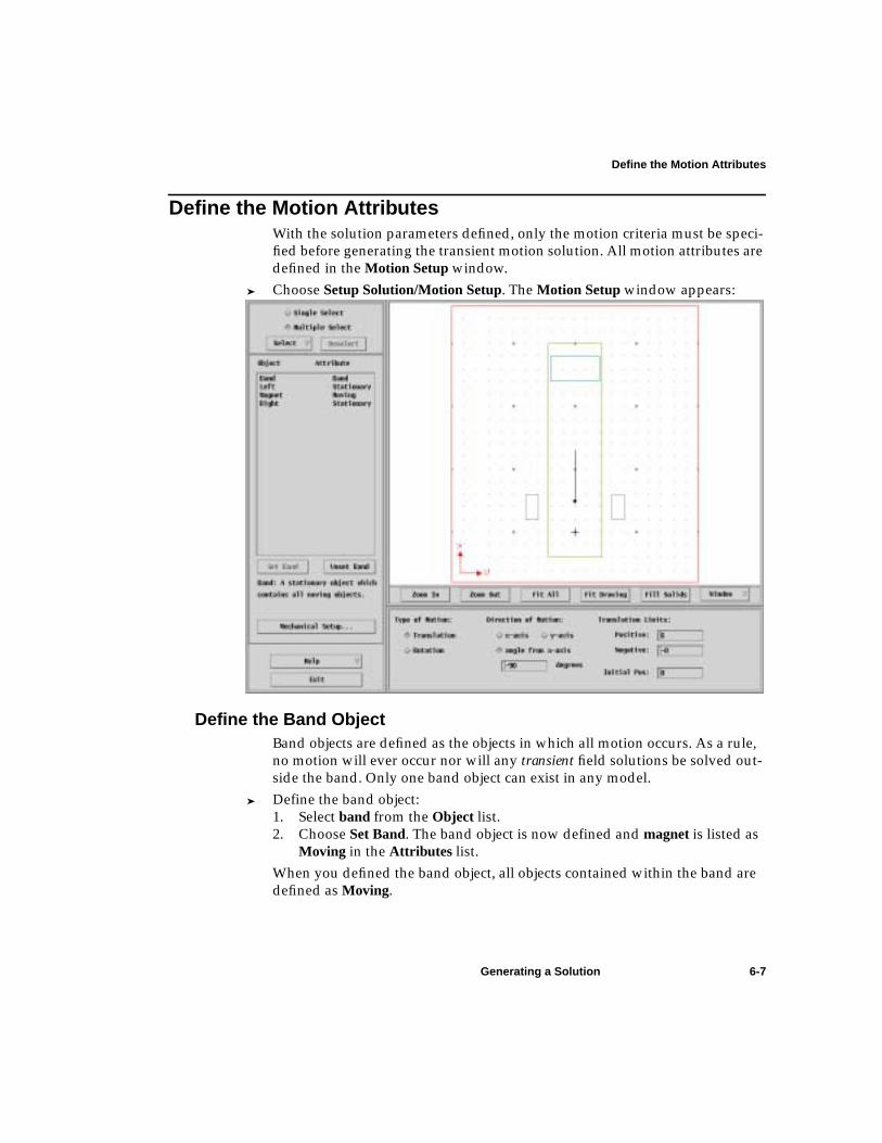
Define the Motion AttributesWith the solution parameters defined, only the motion criteria must be speci-fied before generating the transient motion solution. All motion attributes aredefined in the Motion Setup window.
➤ Choose Setup Solution/Motion Setup. The Motion Setup window appears:
Define the Band ObjectBand objects are defined as the objects in which all motion occurs. As a rule,no motion will ever occur nor will any transient field solutions be solved out-side the band. Only one band object can exist in any model.
➤ Define the band object:1. Select band from the Object list.2. Choose Set Band. The band object is now defined and magnet is listed as
Moving in the Attributes list.When you defined the band object, all objects contained within the band aredefined as Moving.

Define the Motion Attributes
6-8 Generating a Solution
Define the Moving ObjectMoving objects must reside in the band object. In this model, the magnet fallsin the band at a deviation of -90 degrees from the x-axis to cause an oscillationof motion. Because the magnet was present inside the band object at the timethe band was defined, it was automatically assigned the Moving attribute.
➤ Define the motion of the magnet:1. Select Magnet from the Object list.2. Select Translation as the Type of Motion.3. Select angle from x-axis as the Direction of Motion. The degrees field
becomes active.4. Enter -90 in the degrees field.5. Under Translation Limits, do the following:
■ Enter 6 in the Positive limit field.■ Enter 0 in the Negative limit field.This defines the limits of motion to be within six inches of the initial posi-tion.
6. Leave Initial Pos set to 0. This is the initial position of the magnet.
Define the Stationary ObjectsStationary objects can exist anywhere in the model, either inside or outsidethe band object. Placing a stationary object inside the band would allow youto calculate the force and torque on the object, while leaving it outside theband would leave it unaffected by the motion.In this example, both copper bars are stationary.Leave the left and right bars set to their defaults.
Define the Mechanical TransientNow you may define the mechanical setup of the example. Because themotion of the magnet involves a spring effect, you will need to define themotion variables as functions of time.
➤ Define the mechanical transient:1. Choose Mechanical Setup. The Mechanical Setup window appears.2. Choose Functions.The Motion Setup Symbol Table appears.

Define the Motion Attributes
Generating a Solution 6-9
Define the Motion Variables
To simulate the spring effect of the motion, you must define the followingvariables:
Define the Spring Constant
To accurately obtain the restoring force, you must first define the spring con-stant for the motion problem.
➤ Define the spring constant:1. Enter k in the field to the left of the equals sign.2. Enter 11 in the field to the right of the equals sign.3. Choose Add. The k value is added to the table.Define the Weight
Define the weight of the magnet. The magnet’s weight is based on its massand gravity.
➤ Define the weight:1. Enter weight in the field to the left of the equals sign.2. Enter 9.8/2.2 in the field to the right of the equals sign.3. Choose Add. The weight value is added to the table.Define the Restoring Force
➤ Now define the spring-related restoring force:1. Enter spring in the field to the left of the equals sign.2. Enter -k*(P-4) in the field to the right of the equals sign.3. Choose Add. The spring value is added to the table.Define the Damping Coefficient
The damping value is defined as a conditional expression based on the posi-tion, P, of the magnet as it moves. You must define the damping based on thiscondition.
➤ Define the damping value:1. Enter DD in the field to the left of the equals sign.2. Enter if (((P>4)&&(P<=6)),5,0) in the field to the right of the equals sign.
This establishes a condition that if the position falls between four and sixinches, a damping value will be applied. The damping is intended todecrease the magnitude of the oscillation of position over time.
3. Choose Add. The DD value is added to the table.
k The spring constant.DD The damping coefficient.FF The forces based on the weight, damping coefficient,
and the spring constant.spring The spring-related restoring force.weight The weight of the magnet.

Define the Motion Attributes
6-10 Generating a Solution
Define the Forces Factor
Like the damping value, the forces value is also conditional, based on theposition, weight, and spring constant.
➤ Define the forces value:1. Enter FF in the field to the left of the equals sign.2. Enter if (((P>4)&&(P<=6)),weight+spring,weight) in the field to the right of
the equals sign.3. Choose Add. The FF value is added to the table.4. Choose Done. The table vanishes.Define the Mechanical Transient
Now you can use the function values to define the physical parameters.➤ Define the mechanical transient:
1. Select Consider Mechanical Transient if it is not already selected. Fieldsappear, allowing you to define the velocity, mass, damping, and loadforce of the system.
2. Leave 0 in the Initial Velocity field.3. Enter 0.4545 for the Mass of the moving object.4. Choose Options. The Options window appears.5. Select both Damping and Load from the list. This defines both parameters
as having functional values.6. Choose OK. The Options window closes. You return to the Mechanical
Setup window.7. Enter DD in the Damping field. This is the functional value you defined
for the damping.8. Enter FF in the Load Force field. This is the functional load force value
you defined in the Motion Setup Symbol Table.9. Choose OK to close the Mechanical Setup window.You return to the Motion Setup window.
Exit the Motion Setup WindowWith the motion completely defined, you are ready to exit the Motion Setupwindow and solve the problem.
➤ Exit the Motion Setup window:1. Choose Exit. A window appears, prompting you to save your changes
before exiting.2. Choose Yes.The Motion Setup window closes.

Generate the Solution
Generating a Solution 6-11
Generate the SolutionNow that you’ve set up the solution parameters, the problem is ready to besolved. Depending upon how closely you followed the guide, the results thatyou obtain should be approximately the same as the ones given in the follow-ing sections.
➤ Execute the solution now as follows:● Choose Solve/Nominal Problem. The solution process begins and the
following things happen:■ The system creates the initial finite element mesh for the structure. A
bar labeled Making Initial Mesh appears in the Solution Monitoringbox at the bottom of the screen. It shows the system’s progress as itgenerates the mesh.
■ Buttons labeled Abort, Stop, and Refresh appear next to the progressbar and remain there throughout the entire solution process. Ifdesired, you can use them to abort the solution process, temporarilystop the solution generation, or refresh the plots in the window. If theconvergence panel is displayed, choosing Refresh plots the tangentialforce of the model and lists the available parameters for plotting.
■ A bar labeled Setting up solution files appears.After the system makes the initial finite element mesh, the motion solutionprocess begins.
Monitoring the SolutionThe Solving for Transient monitoring bar appears in the Solution Monitoringbox at the bottom of the menu. This allows you to monitor the simulator’sprogress as it computes the required time steps.
☞Note: The solutions given in this guide were computed on a SPARCstation 2
workstation. Depending on the platform and available memory, youranswers may differ slightly from those presented.

Completing the Solution Process
6-12 Generating a Solution
Completing the Solution ProcessWhen the solution is complete, a window with the following messageappears:
Solution Process is complete
➤ Choose OK to continue.You are now ready to view the completed solution.
☞Note: After a solution is generated, the system does not allow you to change
the geometry, material properties, mesh, or boundary conditions of themodel unless you first delete the solution. Therefore, you must generatea new solution if you change the model after generating a solution.
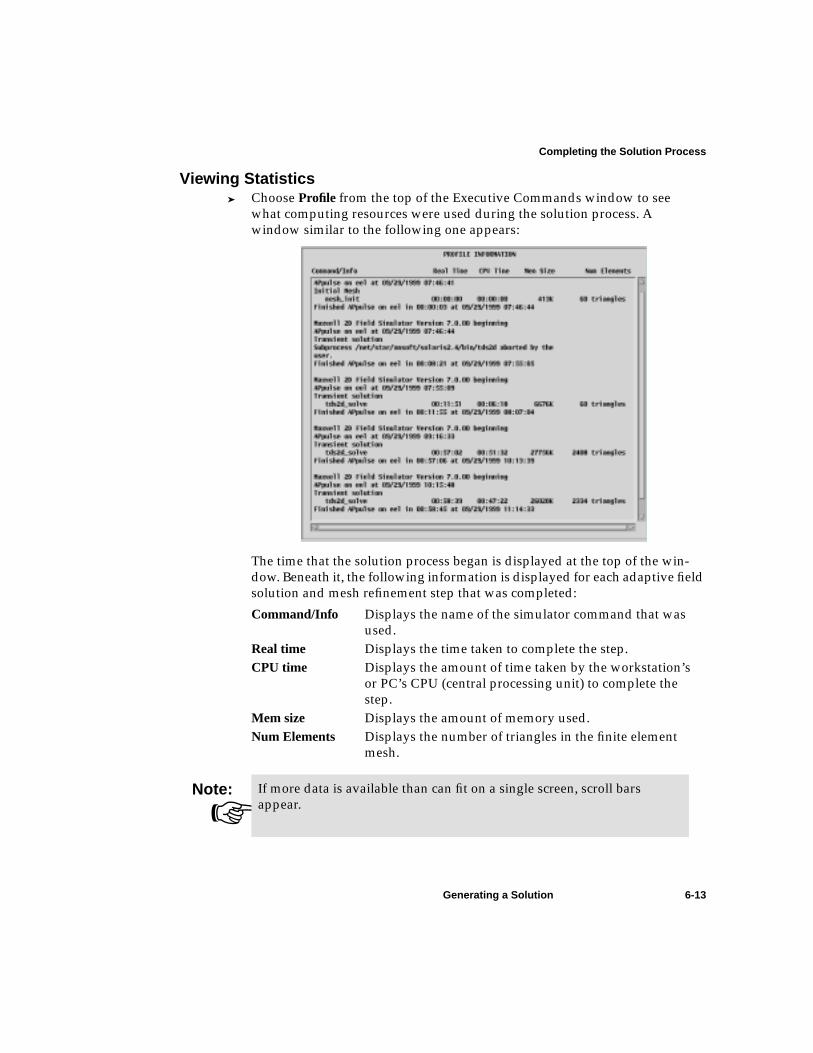
Completing the Solution Process
Generating a Solution 6-13
Viewing Statistics➤ Choose Profile from the top of the Executive Commands window to see
what computing resources were used during the solution process. Awindow similar to the following one appears:
The time that the solution process began is displayed at the top of the win-dow. Beneath it, the following information is displayed for each adaptive fieldsolution and mesh refinement step that was completed:
Command/Info Displays the name of the simulator command that wasused.
Real time Displays the time taken to complete the step.CPU time Displays the amount of time taken by the workstation’s
or PC’s CPU (central processing unit) to complete thestep.
Mem size Displays the amount of memory used.Num Elements Displays the number of triangles in the finite element
mesh.
☞Note: If more data is available than can fit on a single screen, scroll bars
appear.
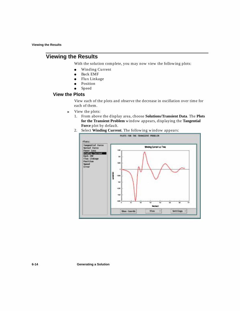
Viewing the Results
6-14 Generating a Solution
Viewing the ResultsWith the solution complete, you may now view the following plots:● Winding Current● Back EMF● Flux Linkage● Position● Speed
View the PlotsView each of the plots and observe the decrease in oscillation over time foreach of them.
➤ View the plots:1. From above the display area, choose Solutions/Transient Data. The Plots
for the Transient Problem window appears, displaying the TangentialForce plot by default.
2. Select Winding Current. The following window appears:

Viewing the Results
Generating a Solution 6-15
3. Select Back EMF. The following window appears:
4. Select Flux Linkage. The following window appears:

Viewing the Results
6-16 Generating a Solution
5. Select Position from the Plots list. The following plot appears:
6. Select Speed. The following window appears:
Now you are ready to analyze the transient solutions.

Analyzing the Solution 7-1
7
Analyzing the Solution
Now that you have generated the transient solution for the motion problem,you can analyze it using the post-processing features of Maxwell 2D.Your goals for this chapter are as follows:● Plot the results of the induced current and flux density for the saved time
steps.● Use the plane calculator to derive the induced current from the current
density.
Time: The total time needed to complete this chapter is approximately 35 min-utes.

Post Process the 0.1-second Time Step
7-2 Analyzing the Solution
Post Process the 0.1-second Time StepUse the 2D Post Processor to plot quantities and access the calculator menus.For this problem, you will plot the current and flux density values at 0.1 and0.3 seconds.
Access the Post ProcessorYou must access the 2D Post Processor before selecting the time steps youwish to analyze.
➤ Access the 2D Post Processor and select the time step:1. Choose Post Process/Fields. The following window appears, listing both
the saved time steps and their respective directories:
2. Select 0.1 from the Time list.3. Choose Post Process.The 2D Post Processor window appears:

Post Process the 0.1-second Time Step
Analyzing the Solution 7-3
Post Processor Screen LayoutThe following sections provide a brief overview of the Post Processor in Max-well 2D. For more details, refer to the Maxwell 2D online documentation.
General Areas
The 2D Post Processor is divided into the following general areas:
Executing Commands
Use the mouse to access, execute, and abort Post Processor commands. Unlikethe other software module windows in Maxwell 2D, you cannot access com-mands via a tool bar or hotkeys.
Project Window
The outermost window in the post processor is called the project window.The project window contains the geometry for a specific project and displays2D Post Processor and the output directory name, out0, in its title bar. Bydefault, one subwindow is contained within the project window.
Subwindows
Subwindows, or view windows, are the windows in which you display plots.Up to eight subwindows may be displayed within the project window, allow-ing you to display different plots in each subwindow. For the sample prob-lem, however, the single subwindow is in the project window, which issubwindow 3 by default.
Menu Bar Appears at the top of the Post Processor window. Gener-ally, it is set up the same way as the 2D Modeler’s menubar.
Project Window Contains the geometry and subwindow(s), allowing youto view the model and plots.
Status Area Displays the following information:● Version number of the 2D Post Processor.● “snap-to-point” behavior of the mouse.● Maximum and minimum values of x- and y-
coordinates of displayed objects.● Coordinates of cursor.● Current unit of length.● Mouse button functions.
☞Note: The Post Processor can only display one project window at a time.
Therefore, because each project requires a separate project window, onlyone project can be opened in the post processor at any given time.

Post Process the 0.1-second Time Step
7-4 Analyzing the Solution
Plotting the 0.1-second Flux DensityNow you are ready to plot the B fields. Use the Plot Menu as follows to plotthe flux throughout the problem region at 0.1 seconds.
➤ Plot the flux:1. Choose Post/Plot. The Plot Menu appears:
2. Set Mag B under Value to Yes. Because you may only plot one value at atime from this window, all other values in the list are set to No when youchoose this.
3. Set Shaded under Plot type to Yes, if it is not already set.4. Set Plane under Location set to Yes, if it is not already set.5. Leave Window 3 under Window set to Yes. (By default, the single window
displayed is referred to by the simulator as window 3.)6. Set Spectrum to Yes.7. Set Better Hardcopy to Yes. This creates a more detailed plot for the flux.8. Choose Execute to plot the flux density for the 0.1-second time step. The
Shade Plot window appears, displaying a status bar as the shade plot isgenerated. When the plot window closes, the following plot appears, dis-

Post Process the 0.1-second Time Step
Analyzing the Solution 7-5
playing both the flux density and the color scale of corresponding values:
☞Note: If you wish, you can change the number of divisions for this plot using
the Post/Plane/Shade command. For more details, refer to the Maxwell 2Donline documentation.

Post Process the 0.1-second Time Step
7-6 Analyzing the Solution
CalculatorsTo calculate the induced current, use the solution calculators that allow you tomanipulate the field quantities. All functions of the following three calcula-tors are described in the Maxwell 2D online documentation.
Plane Calculator
The plane calculator allows you to manipulate field quantities using a stack ofregisters, each of which is able to hold a separate field quantity. For example,to manipulate voltage, you must first load that field into a plane register, thenyou can manipulate the field using the various plane calculator commands.
Line Calculator
The line calculator allows you to map values from a plane register onto a lineand to perform operations such as integration over that line. Like the planecalculator, the line calculator can be visualized as a stack of registers, exceptthat these registers are one-dimensional, containing field values only at pointsalong the line you select.
Number Calculator
The number calculator allows you to manipulate a stack of numbers. Use theregisters in this calculator to store the scalar results of operations such as lineintegrals.
☞Note: Regardless of the current unit of length, the simulator expresses all out-
put quantities in MKS (SI) units.
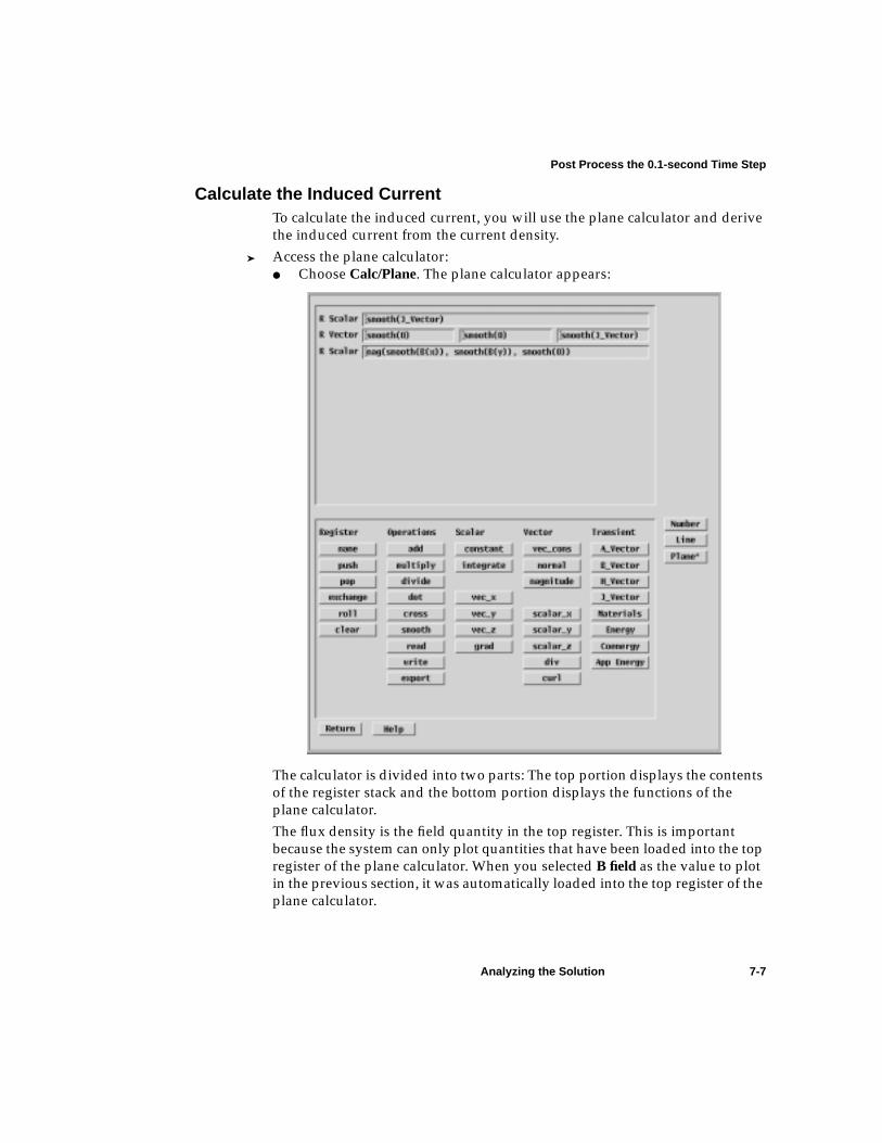
Post Process the 0.1-second Time Step
Analyzing the Solution 7-7
Calculate the Induced CurrentTo calculate the induced current, you will use the plane calculator and derivethe induced current from the current density.
➤ Access the plane calculator:● Choose Calc/Plane. The plane calculator appears:
The calculator is divided into two parts: The top portion displays the contentsof the register stack and the bottom portion displays the functions of theplane calculator.The flux density is the field quantity in the top register. This is importantbecause the system can only plot quantities that have been loaded into the topregister of the plane calculator. When you selected B field as the value to plotin the previous section, it was automatically loaded into the top register of theplane calculator.

Post Process the 0.1-second Time Step
7-8 Analyzing the Solution
Calculate and Plot the 0.1-second Induced CurrentTo plot the induced current for the 0.1-second time step, you must first loadthe current density, J, into the field calculator.
Load and Compute J
The first step in computing the induced current is to load the J vector in thetop register of the stack.
➤ Load the J vector:1. Choose J_Vector to load J into the top register of the plane calculator first.
After J is loaded, the top register appears as follows:R Vector 0 0 J_Vector
The R indicates that the vector value is a real number, as opposed to acomplex number.
2. Choose smooth to refine the value in the top register of the plane calcula-tor. Because the vector values are derived from the nodes of the trianglesin the mesh, smoothing the values allows the software to select the bestvalue for the induced current. The top register appears as follows:
R Vector smooth(0) smooth(0) smooth(J_vector)
3. Choose scalar_z. This forces the z-component of the current density tobecome a scalar value.
4. Choose Return.Now you can plot the induced current.
Refresh the Screen
Refresh the window before plotting the induced current. This allows you toplot the values in a clear window, without unnecessary confusion of overlap-ping plots.
➤ Refresh the screen:● Choose Window/Refresh.The window is refreshed and cleared of plotted data.
☞Note: Complex numbers — such as phasor quantities — are not accessible from
the transient solver. They are accessible from the AC Magnetics solvers,however.
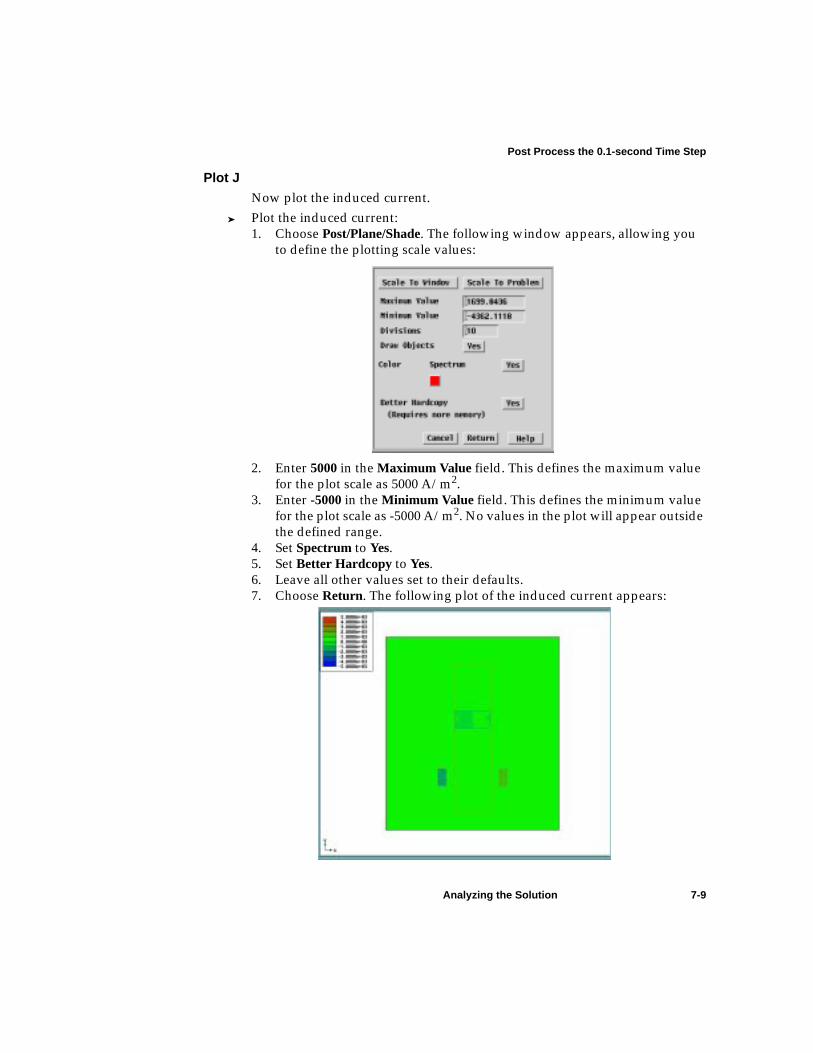
Post Process the 0.1-second Time Step
Analyzing the Solution 7-9
Plot J
Now plot the induced current.➤ Plot the induced current:
1. Choose Post/Plane/Shade. The following window appears, allowing youto define the plotting scale values:
2. Enter 5000 in the Maximum Value field. This defines the maximum valuefor the plot scale as 5000 A/m2.
3. Enter -5000 in the Minimum Value field. This defines the minimum valuefor the plot scale as -5000 A/m2. No values in the plot will appear outsidethe defined range.
4. Set Spectrum to Yes.5. Set Better Hardcopy to Yes.6. Leave all other values set to their defaults.7. Choose Return. The following plot of the induced current appears:

Post Process the 0.1-second Time Step
7-10 Analyzing the Solution
Return to the Executive Commands WindowOnce the calculations for the 0.1-second time step are complete, you can exitthe post processor and return to the Executive Commands window and postprocess the results for the 0.3-second time step.
➤ To return to the Executive Commands window:1. Choose File/Exit. A window appears, asking you to confirm the exit.2. Choose Yes. The 2D Post Processor window closes.You return to the Executive Commands window.

Post Process the 0.3-second Time Step
Analyzing the Solution 7-11
Post Process the 0.3-second Time StepUse the 2D Post Processor to plot quantities and access the calculator menus.For this problem, you will plot the current and flux values at 0.1 and 0.3 sec-onds.
➤ Access the Post Processor:1. Choose Post Process/Fields. The Post-Process Saved Fields window again
appears, listing both the saved time steps and their respective directories.2. Select 0.3 from the Time list.3. Choose Post Process.4. Again, the 2D Post Processor appears, this time displaying the model for
the 0.3-second time step.Notice that the magnet has fallen significantly from its position in the 0.1-sec-ond time step.
Plotting the 0.3-second FluxNow you are ready to plot the B fields. Again, use the Plot Menu to plot theflux throughout the problem region at 0.3 seconds.
➤ Plot the flux:1. Choose Post/Plot. The Plot Menu appears.2. Set Mag B under Value to Yes.3. Set Shaded under Plot Type to Yes.4. Leave Plane under Location set to Yes.5. Leave Window 3 under Window set to Yes.6. Set Spectrum to Yes.7. Set Better Hardcopy to Yes.8. Choose Execute. A progress bar appears, monitoring the plotting process.
When the progress bar vanishes, the following plot appears:

Post Process the 0.3-second Time Step
7-12 Analyzing the Solution
Calculate and Plot the 0.3-second Induced CurrentAs you did for the 0.1-second time step, first access the plane calculator andload the current density, J, into the field calculator before computing theinduced current.
Load and Compute J➤ Load the J vector:
1. Choose Calc/Plane. The plane calculator appears.2. Choose J_Vector to load J into the top register of the plane calculator first.
After J is loaded, the top register appears as follows:R Vector 0 0 J_Vector
3. Choose smooth to refine the value in the top register of the plane calcula-tor. The top register appears as follows:
R Vector smooth(0) smooth(0) smooth(J_vector)
4. Choose scalar_z. This forces the z-component of the current density tobecome a scalar value.
5. Choose Return.Now refresh the window and plot the induced current for the 0.3-second timestep.
Refresh the Screen
Refresh the window before plotting the induced current for the 0.3-secondtime step.
➤ Refresh the screen:● Choose Window/Refresh.The window is refreshed and cleared of plotted data.

Post Process the 0.3-second Time Step
Analyzing the Solution 7-13
Plot J➤ Plot the induced current:
1. Choose Post/Plane/Shade. The following window appears, allowing youto define the plotting scale values:
2. Enter 2500 in the Maximum Value field.3. Enter -2500 in the Minimum Value field. No values in the plot will appear
outside the defined range.4. Set Spectrum to Yes.5. Set Better Hardcopy to Yes.6. Leave all other values set to their defaults.7. Choose Return. The following plot appears:

Exit Maxwell 2D
7-14 Analyzing the Solution
Exit Maxwell 2DOnce you have finished with the post processing functions, you are ready toexit the software.
➤ Exit Maxwell 2D:1. Choose File/Exit from the Post Processor. A window with the following
prompt appears:Exit Post Processor?
2. Choose Yes. The Executive Commands window appears.3. Choose Exit from the bottom of the Executive Commands menu. The fol-
lowing prompt appears:Exit from Maxwell 2D?
4. Choose Yes.The Executive Commands window disappears.
Exit the Maxwell SoftwareYou can exit the Project Manager and the Print Manager when you exit theMaxwell Control Panel.
➤ Exit the Maxwell Control Panel:1. Display the Maxwell Control Panel in the foreground.2. Choose Exit. A window with the following prompt appears:
Exit Maxwell?
3. Choose Yes.Now you have exited the Project Manager, Print Manager, and the MaxwellControl Panel. Workstation users now return to the UNIX prompt, and PCusers return to Microsoft Windows.

Index-1
Index
Numerics2D Modeler
accessing 4-3exiting 4-13
2D Post Processor 7-2, 7-11
Aaliases 2-4Assign/Boundary command, Balloon 5-13Assign/Source commands, Solid 5-12
Bbackground
and boundary conditions 5-8ballooning 5-13default material for 5-6excluding from solution region 5-6extending 5-13including in solution region 5-6
band, assigning a material to 5-5bars, applying voltages to 5-11boundary conditions 5-8
and symmetry 5-13changing 5-14
deleting 5-14displaying 5-9, 5-14electrically grounded system 5-13electrically insulated system 5-13for sample problem 5-10screen layout 5-9use of 5-8
Boundary Manager 5-9Boundary Manager, exiting 5-14buttons
choosing 4-3disabled 2-6
CCalc commands, Plane 7-7, 7-12calculators
accessing the plane 7-7, 7-12complex values in registers 7-8display of functions 7-7display of registers 7-7line calculator 7-6menu 7-7number calculator 7-6overview 7-6plane calculator 7-6real values in registers 7-8
capacitance, calculating with solution calculators 7-6
Index-2
Change Dir 2-4charges, and ballooned boundaries 5-13colors, changing for objects 4-8computing resources
and background 5-6viewing 6-13
convergence data, viewing 6-11CPU time 6-13
DDefine Model 3-5, 4-3D-field 7-8, 7-12direct solver 6-5directories
project 4-1selecting project 2-5
dot product calculations 7-9Draw Model 3-5Drawing 3-5drawing plane 4-2drawing region
adjusting view of 4-13setting up 4-6
EEdit/Attributes/Rename command 4-12Edit/Duplicate/Along Line command 4-11Edit/Select commands 4-11Edit/Select/Object commands 5-13E-field 7-8, 7-12electric fields 5-10electric scalar potential
and electric fields 5-10plotting 7-4
Electrostatic 4-2electrostatic solver 4-2Executive Commands menu
Define Model 4-3Post Process 7-2, 7-11Setup Boundaries/Sources 5-8Setup Materials 5-3Setup Solution 6-1
Solve 6-11Solver 4-2
executive commands menu 3-3executive commands window 3-3
Ffield of view, fitting all objects in 4-13field quantities
dot products of 7-9loading into registers 7-6, 7-8, 7-12manipulating with solution calculators 7-6plotting 7-4real versus complex 7-8
File commands, Exit 4-13Fit All 4-13
Ggeometric models, general strategy for creating 4-3geometry, sample problem model 1-3ground plane, assigning a material to 5-5grounded system 5-13Group Objects 3-5, 4-13
IICCG solver 6-5insulated system 5-13
Kkeyboard
selecting points with 4-8using hotkeys 4-5
Lline calculator 7-6lines, for use as registers 7-6

Index-3
Mmagnet, assigning a material to 5-4material database
adding materials to 5-2global versus local 5-3
Material Manager, accessing 5-3materials
adding to database 5-2assigning to microstrips 5-5assigning to objects 5-2assigning to the background 5-6assigning to the ground plane 5-5assigning to the substrate 5-4attributes 5-4global 5-3global versus local database 5-3screen layout 5-3
Maxwell 2Dexecutive commands 3-5general procedure 3-5model window 3-3
Maxwell 2D Modeler 4-3accessing menu commands 4-4layout 4-4project windows 4-5subwindows 4-5tool bar 4-4
Maxwell Control Panel, accessing 2-2Maxwell Control Panel commands, Projects 2-3memory size 6-13mesh
and solution accuracy 6-3default 6-3example of 1-2initial 6-11starting 6-3use of 1-2
message bar 6-11Model/Drawing Units command 4-6modeling
creating the geometry 4-7drawing microstrips 4-10
using the keyboard 4-7
Nnames
changing for objects 4-8, 4-12defining object names 4-8
number calculator 7-6
OObject commands, Rectangle 4-8objects
assigning materials to 5-2attributes of 4-12changing the colors of 4-8changing the names of 4-8, 4-12copying 4-11creating 4-7, 4-8rectangles 4-8
Pplane calculator 7-6planes, for use as registers 7-6Plot 7-4plots
common quantities 7-4equipotential contours 7-4from calculator registers 7-7
pointsentering from the keyboard 4-8selecting with the mouse 4-8
Post Process 3-6, 7-2, 7-11post processing 7-2, 7-11
plotting results 7-4post processing, screen layout 7-3
project window 7-3subwindows 7-3
post processor, screen layout 7-3Post/Plot command 7-4project alias 2-4project directory
adding 2-4

Index-4
creating 2-3definition of 2-3
Project Manager commandsChange Dir 2-4Projects 2-3
Project Manager optionsNew 2-5Save Notes 2-6
Projects 2-3projects
creating 2-5entering descriptions of 2-6naming 2-5project notes 2-6selecting and accessing 2-5selecting project type 2-5
RRectangle 4-8registers
complex values in 7-8in the line calculator 7-6in the number calculator 7-6in the plane calculator 7-6loading values into the plane 7-8, 7-12real values in 7-8
residual 6-5
Ssaving geometry files 4-13scientific notation 6-6Setup Boundaries/Sources 3-5, 5-8Setup Executive Parameters 3-5, 6-6Setup Materials 3-5, 5-3Setup Solution 3-6, 6-1solution monitoring area 3-3solutions
analysis 7-1calculated values 6-3computing 6-11convergence 6-11CPU time 6-13
criteria for computing 6-3effect of mesh 6-3generating 6-11interpolated values 6-3interrupting 6-11memory used 6-13monitoring 6-11plotting 7-4real time used 6-13satisfying equations 6-5types 6-6
Solve 3-6, 6-11Solver 3-5, 4-2solver choice 6-5solver residual 6-5solver type 4-2solvers
auto 6-5direct 6-5ICCG 6-5
sources 5-8changing 5-14deleting 5-14displaying 5-9, 5-14for sample problem 5-10screen layout 5-9
specifying drawing planes 4-2starting mesh 6-3subwindows 7-3symmetry boundary conditions 5-13
Ttool bar 4-4
Uunits
changing 4-6displaying 4-6rescaling geometric models 4-6

Index-5
Vvoltages
and ballooned boundaries 5-13applying to microstrips 5-11
Wwindows
project windows 7-3subwindows 7-3

Index-6