Title: Numerical investigation of noise generation and radiation from an existing modular expansion joint between prestressed concrete bridges Authors Jhabindra P. Ghimire, Yasunao Matsumoto, Hiroki Yamaguchi and Itsumi Kurahashi Affiliation Department of Civil and Environmental Engineering, Saitama University, 255 Shimo-Ohkubo, Sakura, Saitama, 338-8570, Japan Correspondence address: Yasunao Matsumoto, PhD Department of Civil and Environmental Engineering, Saitama University, 255 Shimo-Ohkubo, Sakura, Saitama, 338-8570, Japan E-mail: ymatsu@mail.saitama-u.ac.jp Telephone: +81 (0)48 858 3557 Fax: +81 (0)48 858 7374

Abstract Noise generated from modular bridge expansion joints during vehicle pass-bys has caused localized environmental problems in Japan and elsewhere. The objective of this study was to understand the mechanism of noise generation and radiation from a modular expansion joint installed in an expressway bridge. A numerical investigation was conducted in order to understand the dynamic characteristics of the joint and the acoustic characteristics of the sound field around the joint that measurements cannot reveal due to their limitations, such as the number of measurement locations that are required. Vibro-acoustic analysis was conducted by using the finite element method–boundary element method (FEM–BEM) approach: dynamic analysis of the joint was carried out by FEM and the sound fields inside the cavity located beneath the joint and outside of the cavity were analyzed by BEM. It was concluded that dominant frequency components in the sound pressure inside the cavity were due to excitation of the structural modes of the joint and/or acoustic modes of the cavity. For the expansion joint investigated, the sound field farther than about 35 m from the joint–cavity center could be considered as far field in the range 50–400 Hz. Keywords: modular bridge expansion joint; FEM–BEM approach; sound generation mechanism; far field

1. Introduction Bridge expansion joints serve to permit the static and dynamic deformations of bridge decks caused by various external effects, such as thermal changes, traffic loading, wind, and earthquake. Requirements for expansion joints have become more sophisticated as bridge technology has developed. Bridges with long spans or continuous-type spans require expansion joints which bridge larger gaps than those of ordinary single-span bridges. Curved bridges and base-isolated bridges require expansion joints which can cope with the multi-dimensional movements of bridge decks. Modular bridge expansion joints can allow greater movements in translation and rotation than ordinary expansion joints, such as finger-type joints. A typical modular expansion joint consists of a set of several parallel steel I-beams (referred to as center beams in this paper) aligned perpendicular to the longitudinal axis of the bridge, which is supported by a set of several parallel steel H-beams (referred to as support beams) in parallel with the axis of the bridge. This structure allows the total movement required for the joint to be divided into small movements which need to be accommodated by each gap between the center beams. Because of this advantage, modular bridge expansion joints have been increasingly used on road bridges. However, it has been recognized that the modular bridge expansion joints may cause noise during vehicle pass-bys [1], which sometimes causes localized environmental problem. Ancich and Brown [2] have reported that noise generated by the impact of a motor vehicle on a modular bridge expansion joint can propagate over a long distance and is audible up to 500 m from a bridge in a semi-rural environment. Although, some methods to reduce noise generated from the modular expansion joint have been reported [3], the mechanism of noise generation and radiation from the modular bridge expansion joint has not yet been understood fully. Barnard and Cuninghame [4] have mentioned the possible contribution of the acoustic resonance of the cavity located beneath the joint to noise while vehicles pass over the joint. There have been studies of the mechanism of noise generation from modular expansion joint by using a full-scale joint model [5, 6]. It was concluded from these studies that the noise generated from the top side of the joint may be related to resonances of the air within the gap formed by the rubber sealing between two adjacent center beams and the car tire. The noise generated from the bottom side of the joint was attributed to sound radiation from vibrations of the joint structure, such as the center beams. Since vibrations of the joint structure appeared to be related to the noise generated from the bottom side of the joint, understanding of the dynamic characteristics of the joint structure is useful to develop effective measures for noise reduction. There have been a few studies on the dynamic response of the modular expansion joint to traffic loading, although the objectives of these studies were to investigate the durability of the joint structure exposed to repeated dynamic loadings due to vehicle pass-bys. In an analytical study by Steenbergen [7], a mathematical model of an expansion joint was developed to identify the dynamic characteristics of the expansion joint including the

frequency response function and dynamic amplification factors. The importance of dynamic amplification factors in the design of the expansion joints was highlighted. The natural modes and operational response modes of vibration of the expansion joint installed in a highway bridge were identified in an experimental study by Ancich et al. [8]. In addition, measurements of static and dynamic strain were carried out to assess the fatigue performance of the expansion joint. In relation to the mechanism of noise generation from the bottom side of modular expansion joint, Ancich and Brown [2] have discussed the possibility that the structural vibration modes of the joint and acoustic modes of a cavity located beneath the joint may interact by comparing the natural frequencies of those vibration and acoustic modes. They reported that a Helmholtz absorber installed in the cavity beneath the joint was effective for noise reduction, which implies that the acoustic modes of the cavity may contribute to noise generation. A numerical investigation of the sound field inside the cavity of the full-scale test joint used in previous studies [5, 6] was conducted to understand the generation of noise inside the cavity during vehicle pass-by by Ghimire et al. [9]. The results from numerical analysis using the FEM–BEM approach were compared with experimental results from impact testing. The study showed that the dominant frequency components in the noise inside the cavity were due to the excitation of structural modes of the joint and/or excitation of acoustic modes of the cavity. However, the characteristics of noise radiation from the cavity to the surrounding sound field were not investigated because the full-scale test joint was installed on top of a cavity constructed under the ground. Noise generated from the bottom side of the bridge expansion joint will be radiated from the openings of the cavity beneath the joint possibly due to the propagation of the acoustic modes of the cavity. As far as the authors were aware, the characteristics and mechanism of noise radiation from modular expansion joints have not been studied. Understanding the mechanism of noise generation and radiation from the expansion joint–cavity system is necessary for noise control. The objective of this study was to understand the mechanisms of noise generation and radiation from an existing modular bridge expansion joint installed in an expressway bridge to the surrounding area. First, field measurements of the noise and vibration of the expansion joint under its operating conditions were conducted. A numerical investigation, the main content of the present paper, was then conducted to understand the mechanisms of noise generation and radiation. In the numerical investigation, the modular expansion joint, the cavity and the surrounding sound field were considered to be a vibro-acoustic system. Frequency responses of this system were calculated using the FEM–BEM approach with harmonic dynamic loadings applied to the joint as an input and sound pressures in the sound field around the joint as an output so as to understand the fundamental dynamic and acoustic characteristics of the vibro-acoustic system. The structural modal properties of the joint and the acoustic modal properties of the cavity were obtained in FE analyses of the joint and cavity,

respectively, and used to interpret the frequency responses calculated for the vibro-acoustic system. Additionally, vibration response analysis of the expansion joint to transient loadings on the joint was carried out so as to investigate the relationship of the dynamic responses of the joint under harmonic loadings and transient loadings. The objective of this analysis was to investigate the fundamental characteristics of the dynamic response of the joint to transient loadings. There have been limitations in the numerical analysis conducted with transient loadings in this study. For example, the effect of spatial variation of vehicle loadings on the dynamic response of the joint and the acoustic response of the vibro-acoustic system to the transient loadings have not been investigated due to the limitation of the numerical tools used in this study. Further investigations are required to fully understand the noise generation and radiation from the joint due to real vehicle loadings.

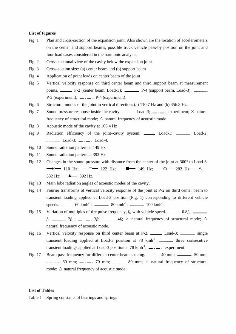
2. Noise and vibration measurement 2.1 Modular expansion joint studied This study has investigated noise generation and radiation from an existing modular expansion joint installed between two prestressed concrete (PC) girder bridges in an expressway. This particular expansion joint was used because the contribution of PC bridges to noise generation was expected to be small due to their relatively heavy mass and also the joint was located in a rural region and there were no other main noise sources. The two-lane bridge was 12.16 m wide. Figure 1 shows the plan and cross-section of the joint. The joint length was the same as the width of the bridge, i.e., 12.16 m. The joint was installed in the bridges in a skewed position such that the angle between the bridge axis and expansion joint axis was 76°. The expansion joint investigated had a single support beam system, which was produced by Kawaguchi Metal Industries Co., Ltd. based on the design by mageba sa: each support beam supported all the center beams. The expansion joint consisted of five center beams that were supported by eight support beams. Control mechanisms consisting of a steel plank (referred to as the control beam) and rubber springs installed between a control beam and the bottom flange of a center beam were designed to prevent excessive displacement between two center beams. Steel frames were placed vertically to accommodate rubber springs and a polyamide bearing between a center beam and a support beam. Polyamide bearings were placed beneath the ends of the support beams and between the support and center beams, as shown in Fig. 1, so as to allow relative movements between the support beams and the bridge girder and relative movements between support beams and center beams, respectively. Similarly, rubber springs were placed on top of the ends of support beams and between the support beams and the frames. The joint also had water and debris drainage capability with the installation of rubber sealing into the gap between two adjacent center beams. There was a cavity beneath the joint between adjacent bridge girders as shown in Fig. 2. The cavity was surrounded by the joint at the top, the bridge girders at the sides, and the concrete pier at the bottom.

FIGURES 1 AND 2 ABOUT HERE

2.2 Measurement and analysis Noise generated when vehicles passed over the expansion joint was measured with sound level meters, RION NL-21 and NL-32. The sound pressure inside the cavity beneath the joint was measured at the center of the cavity at 1.5 m above the floor of the cavity. Sound pressure above the joint was measured with a sound level meter mounted on the parapet wall beside the joint. A sound level meter was placed below the joint on the ground near the pier at 1.5 m above the ground, which was grassy land. To measure the sound radiated outside from the joint–cavity system, two sound level meters were placed at 5 m and 15 m from the edge of the bridge slab. They were placed transverse to the bridge axis and along the longitudinal axis of the cavity beneath the joint. Additionally, the vibration responses of the joint during vehicle pass-bys were measured with piezoelectric accelerometers (RION PV-85) at several locations simultaneously, as shown in Fig. 1. Lateral and vertical accelerations were measured at locations in the first, third and fifth center beams, and only vertical acceleration was measured on the second and third support beams. The lateral direction was defined as the direction perpendicular to the longitudinal axis of the center beam.

Signals from the sound level meters and accelerometers were digitized at 10,000 samples per second after anti-aliasing filtering. Spectral analysis was applied to time histories of sound pressures and accelerations for a period of 0.7 s that included the transient response signals when the front and rear wheels of the vehicle excited the joint. A Hanning window having a length of 0.4096 s was used in the analysis with an overlap of 75% when using the scanning averaging method [10]. The frequency resolution of spectra was therefore 2.44 Hz.

3. Vibro-acoustic analysis of joint–cavity system with harmonic loading 3.1 Finite element model of the joint and its modal properties A three-dimensional FE model of the expansion joint was developed in a similar manner to that used in the full-scale joint model developed in previous studies [6, 9] by using ANSYS 10.0. The center beams, support beams, control beams and frames were modeled with shell elements so that the velocity response of the joint could be transferred directly into the BE analysis of the sound field as the velocity boundary condition. The polyamide bearings and rubber springs were simplified and modeled by using spring elements. The cross-sections of the center beam and the support beam are shown in Fig. 3. Young’s Modulus and Poisson’s ratio of steel components in the joint were 2.06 × 1011 Nm-2 and 0.3, respectively. Material properties of the rubber springs and polyamide bearings used in the joint are shown in Table 1. The maximum size of the FE meshes used in the analysis was 60 mm. The maximum frequency that could be analyzed was 895 Hz, according to the rule of thumb of 6 elements per wavelength, which applies to discussion in the following sections also.

FIGURE 3 AND TABLE 1 ABOUT HERE A total of 663 vibration modes were identified by modal analysis at frequencies below 800 Hz which

was double the maximum frequency of interest, i.e., 400 Hz, in this study. The FE model of the joint structure consisted of several components that had the same geometric and mechanical properties, such as the center beams and the support beams, which may have resulted in many closely spaced modes being identified. It is clear that vehicle pass-bys will not necessarily induce all the vibration modes obtained in the modal analysis.

3.2 Calculation of vibration response The dynamic response of the joint depends on its loading. This has both spatial and temporal characteristics. These are coupled, yielding a transient loading. In this study, the velocity response of the joint was calculated by applying harmonic point loadings to the joint. Although there should be differences between the vibration responses, especially the torsional responses, to transient dynamic loadings caused by different vehicles and the responses to stationary harmonic point loadings, the harmonic loadings were used because of the limitations of the numerical tools used for the acoustic analysis described later in this paper. With the harmonic loadings, the fundamental dynamic and acoustic characteristics of the joint–cavity vibro-acoustic system could be identified so as to assist in understanding the mechanism of noise generation from the joint, although the use of the harmonic point loadings is a limitation of this study. A combination of vertical and lateral harmonic point loads was exerted on the center beams of the joint so as to consider a possible inclined impact of a vehicle tire on the joint. The point loadings were applied to the joint at locations where loadings might be applied during a vehicle pass-by. Figure 1 shows the position of the traffic lanes with a width of 3.5 m on the expansion joint. Figure 1 also shows the names of the structural components of the expansion joint used in this study. Since the joint was installed in a skewed position at an angle of 76° between the joint and bridge axes, as shown in Fig. 1, a vehicle crosses the expansion joint in an inclined orientation. The positions of loading on the two traffic lanes were not considered to be symmetric about the center of the joint as observed in Fig. 1, so the vibration responses of the expansion joint may be different depending on the direction of the traffic. Assuming that a heavy truck with an axle width of 1.8 m passes at the center of a traffic lane, the possible positions of external loading due to a truck pass-by were determined, as shown in Fig. 1. A pass-by of a heavy truck was assumed because the experimental results showed that heavy trucks caused greater vibration responses of the expansion joint. Figure 1 shows that a truck impacts the joint approximately at the middle of adjacent two support beams in the left lane (referred to as Lane 1 in this paper) and near the support beams in the right lane (referred to as Lane 2). Therefore, the loadings were applied at the middle of adjacent two support beams in Lane 1 and near the support beam in Lane 2. Four different load cases were considered in the numerical analysis to calculate velocity responses of the expansion joint as shown in Fig. 1. The point loads were exerted on the central center beam

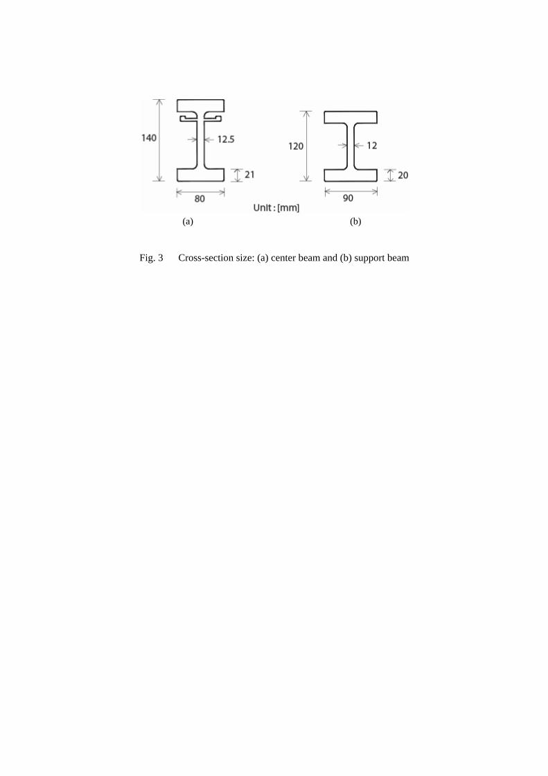
(referred to as the third center beam) at four different positions: (i) between the second and third support beams (Load-1); (ii) between the third and fourth support beams (Load-2); (iii) near the fifth support beam (Load-3); and (iv) near the sixth support beam (Load-4). Only one loading position was considered for each load case given that, when one tire of an axle is on the third center beam, another tire of the same axle is off the joint because of the skewed position of the joint. There were two shell elements in the top flange of the center beam in the direction perpendicular to the joint axis in the FE model so that there were three nodes on the top surface in that direction. The vertical and lateral point loads were applied at the center nodes of those three nodes, i.e., both point loads were applied just above the web of the center beam (Fig. 4). Additionally, the velocity responses of the joint were calculated with harmonic loadings applied at several different positions around those loading positions described above, so as to investigate the effect of the loading position on the vibration responses, because the exact position of the loading during a truck pass-by was not known. Although the results of these calculations are not shown in this paper, the general trend of the vibration response remains similar although there were minor variations in the vibration responses for different loading positions, particularly at higher frequencies.

FIGURE 4 ABOUT HERE Harmonic point loadings with unit amplitude were applied in the frequency range 50–400 Hz at 1 Hz intervals. This range was determined based on the frequency range of the noise generated from the joint–cavity system observed in the measurements. Modal-based forced response analysis was carried out by using the structural modes identified by the modal analysis in the frequency range below 800 Hz by using LMS Virtual.Lab Rev 6A.In general, the highest natural frequency of the structural mode considered in the response calculation should be double the maximum frequency of interest [11]. In the previous studies, the modular expansion joint was found to be lightly damped with a damping ratio less than 3% for most of the lateral and vertical bending modes identified up to 500 Hz from the experiment [6] and less than 2% for all the first four vertical bending modes identified from the experiment [8]. A modal damping ratio of 1% was assumed for all the modes considered in the analysis.

3.3 Boundary element model of the joint–cavity system The sound field around the expansion joint was computed by the indirect boundary element method (IBEM). In the direct BEM, there is a distinction between interior and exterior analysis depending on whether the primary variables are defined on the interior or exterior side of a model. In the indirect method, however, the primary variables, which are layer potentials, contain information about both sides of a boundary surface so that the acoustic medium on both sides of the boundary surface is considered simultaneously. This enables openings and multiple connections to be included in an indirect BE model [12]. Detailed explanations about the BEM can be found elsewhere [12–14]. In the BE model of the joint–cavity system, the boundary of the cavity was discretized by using

quadrilateral and triangular elements. The length of each side of the acoustic BE was 120 mm so that the highest frequency that could be analyzed was 472 Hz. The two openings at the end along the length of the cavity and other small openings between the rubber bearings of the bridge girders were included in the model. The length of the cavity beneath the joint was shorter than the length of the joint. The top boundary of the BE model was made exactly the same as the FE model of the joint so that the velocity response of the joint could be transferred directly to the BE model. The sound speed and the density of the air used in the analysis were 340 ms-1 and 1.225 kgm-3, respectively.

In this analysis, it was assumed that the vibration response calculated from the in vacuo structural modes of the joint calculated separately in the previous section can be used to analyze the acoustic field of the joint–cavity system, i.e., a weak coupling was assumed between the expansion joint and cavity beneath it (vibrations of the expansion joint were not influenced by the fluid), according to the criterion to assess the degree of coupling explained by Kim and Brennan [15]. Layer potentials of the boundary surface were calculated by the IBEM with the velocity responses of the joint calculated to harmonic loadings described in Section 3.2 as a boundary condition. The analysis of the acoustic field was conducted using LMS Virtual.Lab Rev 6A. The layer potentials obtained above were used to calculate the sound pressure at any field point inside the acoustic domain [13]. In this study, field points to calculate the sound pressure were chosen to be identical to the measurement location in the experiment described in Section 2.2.

3.4 Acoustic modal analysis of the cavity beneath the joint In addition to the analysis described above, the cavity beneath the joint was modeled by FE to identify the acoustic modal parameters (i.e., acoustic modes and their corresponding natural frequencies). The acoustic field inside the cavity was modeled by cubical fluid elements of mesh size 130 mm so that acoustic modes having natural frequencies up to 435 Hz could be calculated. The openings at both ends of the cavity length and other small openings between the bearings of bridge girder were modeled by applying the impedance boundary condition: a characteristic acoustic impedance of 416 kgm-2s-1 (corresponding to a sound speed of 340 ms-1 and air density of 1.225 kgm-3) was applied to model these openings.

3.5 Results Figure 5 shows vertical velocity responses calculated with Load-3. The vertical velocity responses calculated at a position in the third center beam between the third and fourth support beams (P-2 in Fig. 1) and at the center of the third support beam (P-4) are shown in Fig. 5. Load-3 in Lane 2 was selected as an example to show the results and used in the interpretation of the experimental results later in this paper. This was because, during the vehicle pass-by experiment, more heavy trucks crossed the joint in Lane 2 than in Lane 1 and, therefore, discussion on the measurements could be

made with more confidence as more experimental data were available for Lane 2 with heavy trucks inducing greater vibration responses.

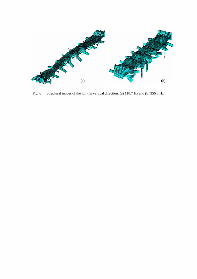
FIGURE 5 ABOUT HERE In the frequency range below 400 Hz, there were several dominant peaks in the vertical velocity responses of the center beams and support beams, which may have corresponded to the excitation of vibration modes of the joint. Figure 5 implies that the motion of the center beams and motion of the support beams were coupled together in some of the peaks observed: for example, at about 110 Hz and 356 Hz, both the velocity response of the center beam and that of the support beam showed a peak. Figure 6 shows the modal shapes of the joint that may correspond to these peaks. In the structural vibration mode at 110.7 Hz shown in Fig. 6(a), almost all parts of the joint move in phase in the vertical direction, while the center beams vibrate out-of-phase in the lateral direction. The maximum amplitude in the vertical direction was observed near the center of the joint. In the vibration mode at 356.8 Hz shown in Fig. 6(b), higher bending/lateral/torsional modes of the center beams with out-of-phase motions within the joint were observed. They may reduce the efficiency of the sound generation.

FIGURE 6 ABOUT HERE Figure 5 also shows an example of the vertical velocity responses of the center and support beams measured at the measurement points shown in Fig. 1 while a heavy truck crossed the joint in Lane 2. The measurement locations of the data shown in Fig. 5 correspond to the locations in the numerical results shown in the figure. Although the loadings applied to the joint in the experiment were not known, they were clearly different from the harmonic loading in the numerical analysis. Thus, although the numerical results cannot be compared directly with the experimental results, some similar trends may be observed between the vibration responses measured experimentally and those calculated numerically. At frequencies around 120 Hz and around 355 Hz, the vertical response of the center beam was comparable with that of the support beam in the numerical analysis and the experiment. In the frequency range 140–180 Hz, the center beam response was greater than the support beam response. The data recorded with other vehicles also showed similar trends to those shown in Fig. 5, although variations were observed possibly because different vehicles had different dynamic loadings and impacted the joint at different locations, depending on the type of vehicle, vehicle speed, and so on. Figure 7 shows the sound pressure at the measurement point inside the cavity, calculated numerically with Load-3. Figure 7 also shows the sound pressure recorded at the corresponding point in the measurement during a heavy truck pass-by in Lane 2 that corresponds to the vibration response shown in Fig. 5. Although the magnitudes of the sound pressure response obtained from the numerical analysis cannot be compared directly with those obtained in the measurements, some similarities were observed in the numerical analysis and the measurement, such as dominant frequency components.

FIGURE 7 ABOUT HERE

4. Discussion 4.1 Dynamic characteristics of the joint The modal analysis of the joint yielded a total of 663 vibration modes at frequencies below 800 Hz, as mentioned above. Similar studies [6, 9] of numerical modeling of the joint have shown reasonable agreements in the modal properties between the numerical and experimental modal analyses. Roeder [16] has conducted a numerical modal analysis of a modular expansion joint in the "single support bar swivel joist design", and reported that "the modes of vibration for this modular expansion joint were closely spaced with hundreds needed to include the predominate portion of the mass in three-dimensional vibration". This may be consistent with the many closely spaced vibration modes identified for the joint in this study. At frequencies around 110 Hz, a vibration mode in which almost all parts of the joint move in phase in the vertical direction was identified for the joint in this study, as shown in Fig. 6(a). This was also confirmed by an approximate calculation of the natural frequency obtained from the mass of the joint and the sum of the vertical stiffnesses of the polyamide bearings, the rubber springs and the support beams. A "translational (bounce/bending) mode" in the vertical direction, in which all parts of the joint vibrated in phase, was identified for a modular expansion joint in a "hybrid design" at 71 Hz by Ancich et al. [8]. The difference in the natural frequency of a similar mode between this study and Ancich et al. [8] might be caused by the differences in the design of the joint. Roeder [16] has stated that the vibration modes of the joint with the lowest natural frequencies "were associated with horizontal movement", which suggests similar characteristics to those of the joint investigated in this study. The lowest order mode of the joint identified in this study was a mode in which the whole body of the joint moved in phase in the lateral direction. This can be understood from the less stiffness of the bearings and rubber springs at the ends of support beams in lateral direction than in vertical direction, as shown in Table 1. Other lowest order modes were also dominated by lateral vibrations of the joint, which may be attributed to weak axis of cross-section of the center beam being the lateral direction, as shown in Fig. 3.

4.2 Sound generation mechanism inside the cavity The peaks in the frequency response function calculated for the sound pressure inside the cavity, as observed in Fig. 7, may be attributed to the excitation of the structural modes of the joint and/or the acoustic modes of the cavity. Sound generation due to the interaction between a vibrating structure and an enclosed acoustic cavity has been discussed elsewhere [15, 17, 18]. Those studies showed that the dominant peaks in the sound pressure inside the cavity could be due to major contribution from the structural modes of the joint with a minor contribution from the acoustic modes of the cavity or vice-versa. These mechanisms were considered to be possible causes of the peak frequency components in the sound pressure inside the cavity beneath the full-scale joint model of modular expansion joint in the previous study [9]. A similar argument can be made in this study for possible

causes of the peaks in the sound pressure observed in the joint–cavity system investigated. For example, the sound pressure peak at 110 Hz observed in Fig. 7 may be attributed mainly to the excitation of a vibration mode of the joint at 110.7 Hz with significant in-phase vertical vibration of the center and support beams, as shown in Fig. 6(a). This hypothesis may be supported by significant vibration response of the joint at about 110 Hz as seen in Fig. 5. The acoustic modal analysis of the cavity beneath the joint showed that there was an acoustic mode at 106.4 Hz shown in Fig. 8. The comparison between the mode shape of the structural mode shown in Fig. 6(a) and the pressure distribution in the top plane of the cavity in the acoustic modes shown in Fig. 8 implies that there may be little interaction between the structural and the acoustic modes: the structural mode was a symmetric mode about the center of the joint while the acoustic mode was asymmetric. In addition, the acoustic mode had a nodal plane that included the location for the pressure calculation. The sound pressures at around 122, 150, 230, 250 and 392 Hz may also be caused by the structural modes and/or the acoustic modes with varying contributions from those modes depending on frequency.

FIGURE 8 ABOUT HERE Figure 7 shows some other peaks in the sound pressure response at frequencies where there were acoustic modes but no corresponding structural modes. This implies that those sound pressure peaks were caused by the acoustic modes alone. Those peaks were observed especially in the higher frequency range where the acoustic modal density was high. For example, the sound pressure peak at around 332 Hz may be due solely to the excitation of acoustic modes, since there were no structural modes of the joint at around this frequency while there were many acoustic modes as shown in Fig. 7.

4.3 Radiation efficiency of the joint–cavity system The radiation efficiency is an index which expresses how effectively a vibrating structure converts mechanical energy into sound energy. The radiation efficiency is defined as the ratio of the active output power to the input power [19]:

i

activeo

WW

efficiencyRadiation ,= (1)

where is the active output power that is the real part of the output power and corresponds to

the average power radiated by the vibrating structure during one vibration cycle. In the IBEM, the active output power is given by:

activeoW ,

∫=S

nactiveo dSvcW *)Re(21

, μρ (2)

where ρ is the density of the acoustic medium, c is the velocity of sound in the medium, μ is the double-layer potential (or jump of pressure) and the complex conjugate of the normal velocity.

in Eq. (1) is the input power, that is the power associated with the mechanical vibration. It is

obtained by integrating the squared normal velocities of the boundary surface as:

*nv

iW

∫∫ ==S

nS

rmsi dSvcdSvcW 22

21 ρρ (3)

where is the root-mean-square value of the local normal velocity boundary conditions, . The

input power depends only on the prescribed velocity boundary conditions. rmsv nv

The sound radiation efficiencies calculated for the joint–cavity system with all four load cases used in this study are shown in Fig. 9. The figure shows that the mechanical power at frequencies below 100 Hz was not converted efficiently into acoustic power. In the frequency range below 100 Hz, the vibration modes of the joint were dominated by lateral vibration of the whole joint structure and the center beams, although the results of modal analysis are not shown in this paper. This implies that the lateral vibration of the joint did not radiate sound efficiently. Vibration modes of any structure below the critical frequency cannot radiate sound efficiently. The critical frequency of the center beam

of the joint in lateral and vertical directions was calculated by using the simplified expression [20]: cf

k

fc64.3

= (4)

where k is the radius of gyration of the second moment of area in meters. The critical frequency of

the lateral vibration of the center beam calculated using Eq. (4) was 180 Hz. The critical frequency of the vertical vibration of the center beam was 67 Hz indicating that all vertical vibration modes above this frequency could contribute to the sound radiation.

FIGURE 9 ABOUT HERE High radiation efficiency was observed in the range from 100–160 Hz. In this frequency range, there were several vertical vibration modes of the joint with significant vibration in both center and support beams (coupled modes) including the whole body-like mode at 110.7 Hz as shown in Fig. 6(a). In these modes, all the center beams vibrated in phase with the support beams. As observed in Fig. 9, the radiation efficiency was low in the range 160–225 Hz. There were vibration modes of the joint with dominant coupled vertical and torsional vibrations of the center beams and less vibration of the support beams. In these vibration modes, the center beams moved out of phase with each other and the acoustic power radiating from different center beams may have been canceling each other out. These characteristics of the vibration modes may have caused low radiation efficiency. The radiation efficiency was high at frequencies above 275 Hz. At such frequencies, the modal density of the acoustic modes of the cavity was high and the interaction between the vibration modes of the joint and many acoustic modes may have caused high sound radiation efficiency.

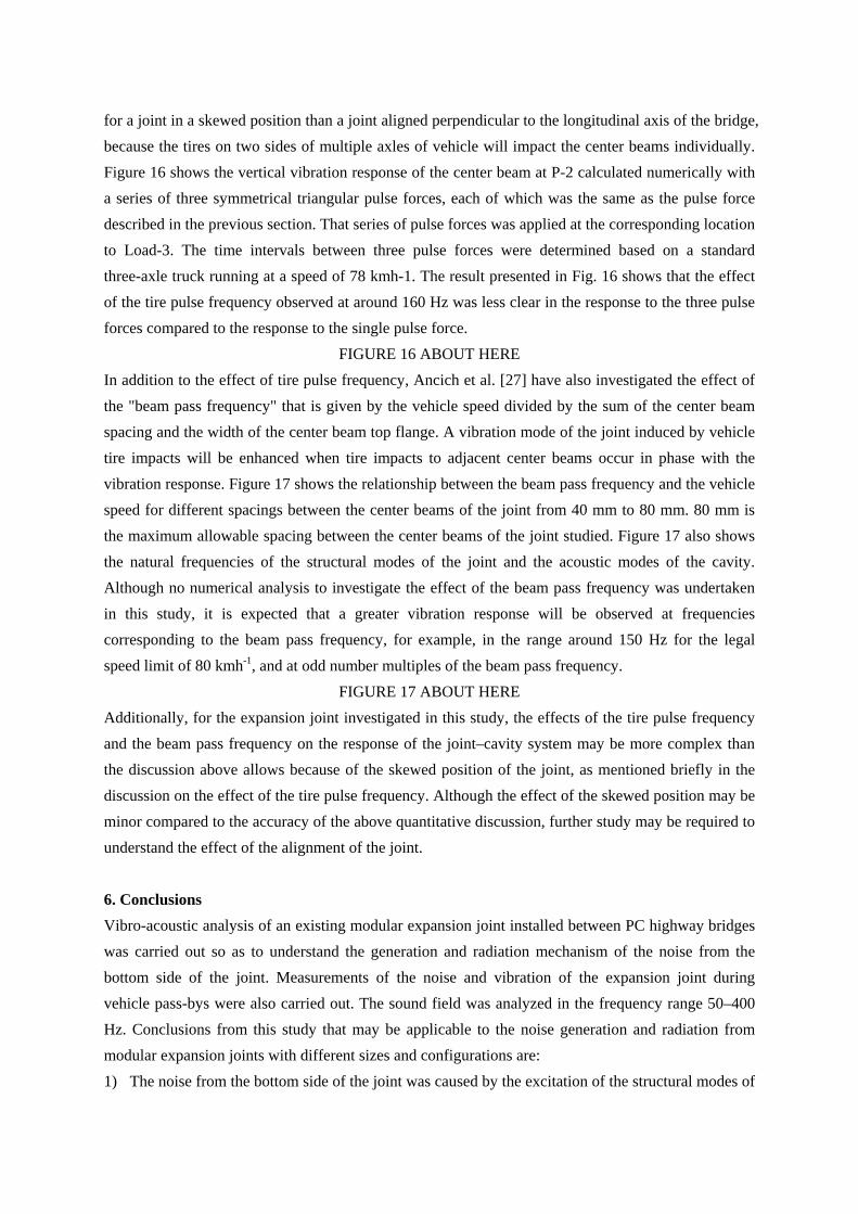
4.4 Effect of distance on directivity of sound radiation It is important to understand the sound radiation characteristics of the joint–cavity system with respect

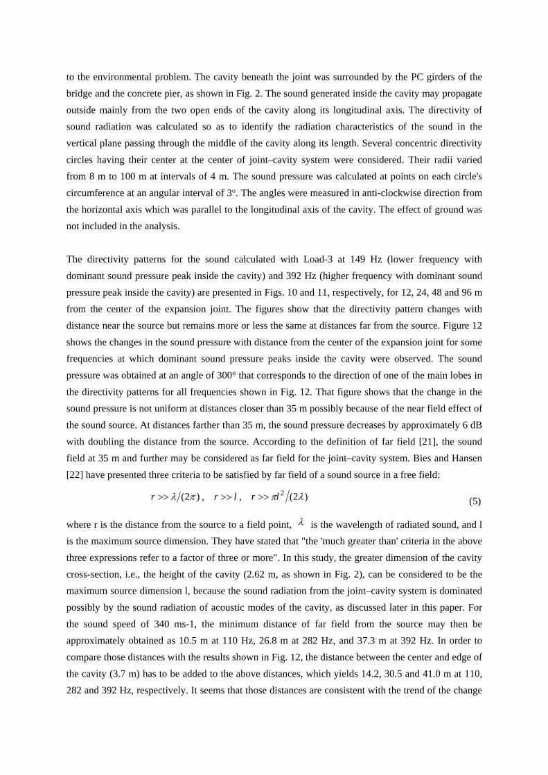
to the environmental problem. The cavity beneath the joint was surrounded by the PC girders of the bridge and the concrete pier, as shown in Fig. 2. The sound generated inside the cavity may propagate outside mainly from the two open ends of the cavity along its longitudinal axis. The directivity of sound radiation was calculated so as to identify the radiation characteristics of the sound in the vertical plane passing through the middle of the cavity along its length. Several concentric directivity circles having their center at the center of joint–cavity system were considered. Their radii varied from 8 m to 100 m at intervals of 4 m. The sound pressure was calculated at points on each circle's circumference at an angular interval of 3°. The angles were measured in anti-clockwise direction from the horizontal axis which was parallel to the longitudinal axis of the cavity. The effect of ground was not included in the analysis. The directivity patterns for the sound calculated with Load-3 at 149 Hz (lower frequency with dominant sound pressure peak inside the cavity) and 392 Hz (higher frequency with dominant sound pressure peak inside the cavity) are presented in Figs. 10 and 11, respectively, for 12, 24, 48 and 96 m from the center of the expansion joint. The figures show that the directivity pattern changes with distance near the source but remains more or less the same at distances far from the source. Figure 12 shows the changes in the sound pressure with distance from the center of the expansion joint for some frequencies at which dominant sound pressure peaks inside the cavity were observed. The sound pressure was obtained at an angle of 300° that corresponds to the direction of one of the main lobes in the directivity patterns for all frequencies shown in Fig. 12. That figure shows that the change in the sound pressure is not uniform at distances closer than 35 m possibly because of the near field effect of the sound source. At distances farther than 35 m, the sound pressure decreases by approximately 6 dB with doubling the distance from the source. According to the definition of far field [21], the sound field at 35 m and further may be considered as far field for the joint–cavity system. Bies and Hansen [22] have presented three criteria to be satisfied by far field of a sound source in a free field:

)2(,,)2( 2 λππλ lrlrr >>>>>> (5)

where r is the distance from the source to a field point, λ is the wavelength of radiated sound, and l is the maximum source dimension. They have stated that "the 'much greater than' criteria in the above three expressions refer to a factor of three or more". In this study, the greater dimension of the cavity cross-section, i.e., the height of the cavity (2.62 m, as shown in Fig. 2), can be considered to be the maximum source dimension l, because the sound radiation from the joint–cavity system is dominated possibly by the sound radiation of acoustic modes of the cavity, as discussed later in this paper. For the sound speed of 340 ms-1, the minimum distance of far field from the source may then be approximately obtained as 10.5 m at 110 Hz, 26.8 m at 282 Hz, and 37.3 m at 392 Hz. In order to compare those distances with the results shown in Fig. 12, the distance between the center and edge of the cavity (3.7 m) has to be added to the above distances, which yields 14.2, 30.5 and 41.0 m at 110, 282 and 392 Hz, respectively. It seems that those distances are consistent with the trend of the change

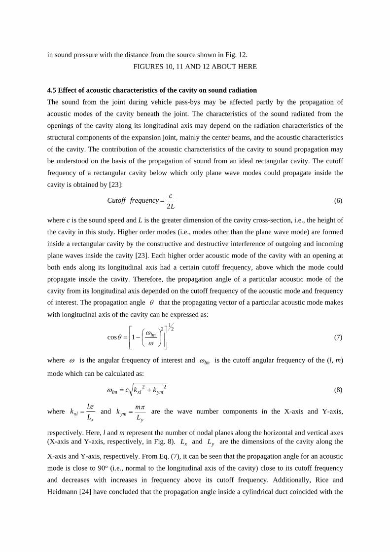
in sound pressure with the distance from the source shown in Fig. 12. FIGURES 10, 11 AND 12 ABOUT HERE

4.5 Effect of acoustic characteristics of the cavity on sound radiation The sound from the joint during vehicle pass-bys may be affected partly by the propagation of acoustic modes of the cavity beneath the joint. The characteristics of the sound radiated from the openings of the cavity along its longitudinal axis may depend on the radiation characteristics of the structural components of the expansion joint, mainly the center beams, and the acoustic characteristics of the cavity. The contribution of the acoustic characteristics of the cavity to sound propagation may be understood on the basis of the propagation of sound from an ideal rectangular cavity. The cutoff frequency of a rectangular cavity below which only plane wave modes could propagate inside the cavity is obtained by [23]:

LcfrequencyCutoff

2= (6)

where c is the sound speed and L is the greater dimension of the cavity cross-section, i.e., the height of the cavity in this study. Higher order modes (i.e., modes other than the plane wave mode) are formed inside a rectangular cavity by the constructive and destructive interference of outgoing and incoming plane waves inside the cavity [23]. Each higher order acoustic mode of the cavity with an opening at both ends along its longitudinal axis had a certain cutoff frequency, above which the mode could propagate inside the cavity. Therefore, the propagation angle of a particular acoustic mode of the cavity from its longitudinal axis depended on the cutoff frequency of the acoustic mode and frequency of interest. The propagation angle θ that the propagating vector of a particular acoustic mode makes

with longitudinal axis of the cavity can be expressed as:

2

12

1cos⎥⎥⎦

⎤

⎢⎢⎣

⎡⎟⎠⎞

⎜⎝⎛−=ωω

θ lm (7)

where ω is the angular frequency of interest and lmω is the cutoff angular frequency of the (l, m)

mode which can be calculated as:

22ymxllm kkc +=ω (8)

where x

xl Llk π

= and y

ym Lmk π

= are the wave number components in the X-axis and Y-axis,

respectively. Here, l and m represent the number of nodal planes along the horizontal and vertical axes (X-axis and Y-axis, respectively, in Fig. 8). and are the dimensions of the cavity along the

X-axis and Y-axis, respectively. From Eq. (7), it can be seen that the propagation angle for an acoustic mode is close to 90° (i.e., normal to the longitudinal axis of the cavity) close to its cutoff frequency and decreases with increases in frequency above its cutoff frequency. Additionally, Rice and Heidmann [24] have concluded that the propagation angle inside a cylindrical duct coincided with the

xL yL

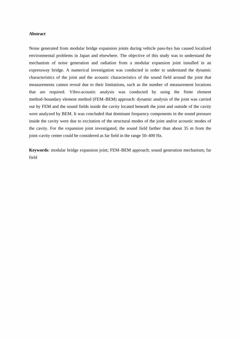
principal lobe of the far field radiation. With respect to the effect of the acoustic characteristics of the cavity beneath the joint on sound propagation, the cutoff frequency of the cavity cross-section was 56 Hz from Eq. (6). The cutoff frequencies of the acoustic modes of the cavity were calculated from Eq. (8) and used to obtain the radiation angle of the main lobe of the acoustic modes in the far field using Eq. (7). The radiation angle of the main lobe of acoustic modes of the cavity of orders (0, 1) to (1, 4) which were present in the frequency range 50–400 Hz are shown in Fig. 13.

FIGURE 13 ABOUT HERE Figures 10 and 11 show that sound radiation pattern of the joint–cavity system depends on frequency. At 149 Hz, as shown in Fig. 10, one of the main radiation lobe in the far field was at approximately 51°. In Fig. 13, the radiation angle of a main lobe in the far field at 149 Hz was 48° for the (0, 2) mode and 20° for the (0, 1) mode. Therefore, the radiation from the (0, 2) mode may be dominant in the radiation at this frequency. At 392 Hz, as shown in Fig. 11, there were many radiation lobes in the far field at different angles from the cavity axis. There was significant sound radiation along the cavity axis (i.e., horizontal direction in the figure) at 392 Hz, unlike at 149 Hz. At frequencies significantly higher than the cutoff frequency of an acoustic mode, the radiation angle of the mode from the cavity axis decreases. Therefore, at high frequencies, the sound could radiate in directions close to the cavity axis by lower order acoustic modes and at greater angles from the cavity axis by acoustic modes having their cutoff frequency close to the frequency of interest. The radiation characteristics at 392 Hz that show many lobes at different angles may be caused by different acoustic modes radiated at different angles as shown in Fig. 13. Radiation from the lower part of the joint within the cavity length may occur through the propagation of the cavity's acoustic modes. Sound radiation from the top and overhanging portion of the joint may have some effect on the radiation patterns of the joint–cavity system.

5. Analysis of joint vibration caused by transient loading Although harmonic loadings applied at a single point were used to calculate the frequency response of the joint–cavity system because of the limitation of numerical tools used in this study, the dynamic loadings on the joint during vehicle pass-bys have temporal and spatial variations in practice. The characteristics of the response of the joint to dynamic vehicle loadings will be different from those to stationary harmonic loadings to some extent. Therefore, in this section, a preliminary investigation of the vibration response of the joint to transient loadings, partly analogous to vehicle loadings, is described. Although a loading on the center beam caused by a vehicle pass-by has spatial and temporal variation, spatial variation of loading was not considered in this analysis for simplicity, which is a limitation of this study.

5.1 Analysis method

The loading on the joint from a vehicle is due to the impacts between tires and the joint structure. The characteristics of tire impact loading on the center beam of the joint will depend on various factors such as: type of vehicle, vehicle speed, tire contact length, and the width of the top flange of the center beam. In previous numerical studies of fatigue of the modular expansion joint, tire impact loading on a center beam was modeled by a symmetrical triangular pulse [16] and a half-cycle sine pulse [25], by assuming a constant vehicle speed. Steenbergen [7] discussed that half-cycle sine pulse was not an exact model of transient vehicle load and suggested a more exact load description in both space and time. In this study, a symmetrical triangular pulse force was used for simplicity. The effect of a possible dynamic interaction between vehicle and joint structure was not considered, as in previous studies [16, 25]. This may be a reasonable assumption because the frequency range of interest in noise generation is much higher than the natural frequencies of vibration modes of the vehicle with a significant modal mass, such as bounce mode and axle-hop mode [26], which will have an effect on the vehicle loading. The duration of the tire impact loading on a center beam of the joint, , was calculated by dividing the sum of the tire contact length, , and the width of the top flange of the center beam, , by the

vehicle speed, v [7, 16, 25]:

dt

cL fb

v

bLt fcd

+= (9)

The reciprocal of the duration of the tire impact loading, , was referred to as the "tire pulse

frequency" by Ancich et al. [27]. In this study, while the tire contact length was assumed to be 0.20 m and the width of the top flange of the center beam was fixed at 0.08 m (Fig. 3), the vehicle speed was in the range 50–100 kmh-1. A unit maximum magnitude was used for the symmetrical triangular pulse forces in the analysis.

dt

The above defined loading in the vertical direction was applied on the third center beam at the same locations as in the analysis with harmonic loadings described in the preceding section: a single pulse force was applied at a location to obtain the vibration response of the joint so as to understand the fundamental characteristics of the joint response to transient loading. As in the harmonic loading analysis, spatial variation of the force in the top flange of the center beam during vehicle pass-by was not considered in the analysis. The model of the joint was exactly the same as the model used in the analysis with harmonic loadings. Transient analysis was carried out using the modal superposition technique in ANSYS 10.0. The structural modes of the joint that were identified in the preceding section were used in the analysis. The integration time step was 0.0002 s so that the frequency range in the analysis was limited to 250 Hz and below to reduce computational load.

5.2 Vibration response of the expansion joint to transient loading Figure 14 shows the spectra of the velocity responses of the joint at P-2 (Fig. 1) calculated in the

transient analysis with the loadings corresponding to vehicle speeds of 60, 80 and 100 kmh-1 applied at Load-3 position. The figure clearly shows that the dynamic response of the joint was dependent on the vehicle speed. The differences in the response caused by the loadings corresponding to different vehicle speeds may be attributed to the effect of the duration of loading.

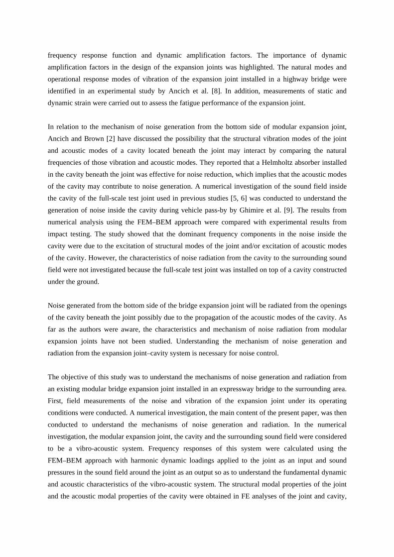
FIGURE 14 ABOUT HERE The relationship between the duration of loading and the response of a single-degree-of-freedom (SDOF) system for a symmetrical triangular pulse loading has been discussed in some textbooks [10, 28]. It is understood that a vibration mode will be excited efficiently when the ratio of the duration of loading, td, to the natural period of the system, Tn, and, in other words, the ratio of the natural frequency of the system, Fn, to the tire pulse frequency, ft, are close to odd numbers. When a vibration mode satisfies the ratios td/Tn and Fn/ft by being close to even numbers, the vibration mode will not be excited efficiently. These characteristics were observed in the velocity responses of the joint calculated shown in Fig. 14. For example, for a vehicle speed of 60 kmh-1, the ratios td/Tn and Fn/ft are about 3 for the natural frequency, Fn, of 178 Hz, and about 2 and 4 for Fn of 119 and 238 Hz, respectively. It seems that these frequencies correspond to a peak frequency of about 173 Hz and trough frequencies of about 118 and 238 Hz in the velocity response calculated for a vehicle speed of 60 kmh-1 shown in Fig. 14. A similar argument can be made for the results with 80 and 100 kmh-1 shown in the figure. Figure 15 shows the relation between the vehicle speed and the tire pulse frequency multiplied by integers from 1 to 4. It also shows the natural frequencies of the structural modes of the joint and the acoustic modes of the cavity. The natural frequency Fn that satisfies the ratios td/Tn and Fn/ft being integers from 1 to 4 can be found for different vehicle speeds. Figure 15 also shows the relationship between the vehicle speed and the tire pulse frequency multiplied by 0.8, because the maximum response of the SDOF system will be induced when the ratios td/Tn and Fn/ft are about 0.8. The figure indicates that, within the range of vehicle speed practically expected, the tire pulse frequency can be a factor affecting the dynamic response of the joint, as discussed elsewhere [27].

FIGURE 15 ABOUT HERE Figure 16 compares the vertical vibration responses of the center beam at P-2 calculated numerically with the harmonic loading Load-3 and the transient loading applied at Load-3 position calculated for a vehicle speed of 78 kmh-1. The figure also shows the experimental data measured at P-2 during a truck pass-by at 78 kmh-1, which are the same data as those shown in Fig. 5. Although the magnitude of the spectra cannot be compared to each other in the figure because each spectrum has different physical meanings, the effect of the tire pulse frequency observed in the response to the transient loading, i.e., a trough at around 160 Hz, was not found in the response to the harmonic loading, as expected. The effect of the tire pulse frequency was not clear also in the experimental data, possibly because the numerical analysis did not account for multiple loadings caused by the multiple tires of vehicle. Additionally, the effect of the tire pulse frequency may appear in more complicated manner

for a joint in a skewed position than a joint aligned perpendicular to the longitudinal axis of the bridge, because the tires on two sides of multiple axles of vehicle will impact the center beams individually. Figure 16 shows the vertical vibration response of the center beam at P-2 calculated numerically with a series of three symmetrical triangular pulse forces, each of which was the same as the pulse force described in the previous section. That series of pulse forces was applied at the corresponding location to Load-3. The time intervals between three pulse forces were determined based on a standard three-axle truck running at a speed of 78 kmh-1. The result presented in Fig. 16 shows that the effect of the tire pulse frequency observed at around 160 Hz was less clear in the response to the three pulse forces compared to the response to the single pulse force.

FIGURE 16 ABOUT HERE In addition to the effect of tire pulse frequency, Ancich et al. [27] have also investigated the effect of the "beam pass frequency" that is given by the vehicle speed divided by the sum of the center beam spacing and the width of the center beam top flange. A vibration mode of the joint induced by vehicle tire impacts will be enhanced when tire impacts to adjacent center beams occur in phase with the vibration response. Figure 17 shows the relationship between the beam pass frequency and the vehicle speed for different spacings between the center beams of the joint from 40 mm to 80 mm. 80 mm is the maximum allowable spacing between the center beams of the joint studied. Figure 17 also shows the natural frequencies of the structural modes of the joint and the acoustic modes of the cavity. Although no numerical analysis to investigate the effect of the beam pass frequency was undertaken in this study, it is expected that a greater vibration response will be observed at frequencies corresponding to the beam pass frequency, for example, in the range around 150 Hz for the legal speed limit of 80 kmh-1, and at odd number multiples of the beam pass frequency.

FIGURE 17 ABOUT HERE Additionally, for the expansion joint investigated in this study, the effects of the tire pulse frequency and the beam pass frequency on the response of the joint–cavity system may be more complex than the discussion above allows because of the skewed position of the joint, as mentioned briefly in the discussion on the effect of the tire pulse frequency. Although the effect of the skewed position may be minor compared to the accuracy of the above quantitative discussion, further study may be required to understand the effect of the alignment of the joint.

6. Conclusions Vibro-acoustic analysis of an existing modular expansion joint installed between PC highway bridges was carried out so as to understand the generation and radiation mechanism of the noise from the bottom side of the joint. Measurements of the noise and vibration of the expansion joint during vehicle pass-bys were also carried out. The sound field was analyzed in the frequency range 50–400 Hz. Conclusions from this study that may be applicable to the noise generation and radiation from modular expansion joints with different sizes and configurations are: 1) The noise from the bottom side of the joint was caused by the excitation of the structural modes of

the expansion joint and/or acoustic modes of the cavity beneath the joint, which is consistent with an earlier conclusion [9] derived from a full-scale model of a modular expansion joint;

2) The sound radiation efficiency of the joint–cavity system appeared to be high at natural frequencies of vibration modes of the joint with significant vertical vibration of center and support beams;

3) Noise from the joint–cavity system may be propagated most effectively at radiation angles of acoustic modes of the cavity, which can be predicted roughly from the fundamental theory of sound radiation from cavities and waveguides;

4) The boundary between near field and far field in the sound field around the joint–cavity system may be predicted approximately by the previous findings of the characteristics of radiation field of a sound source by considering the greater dimension of the cavity cross-section as the maximum source dimension.

7. Acknowledgement This study was conducted in collaboration with Kawaguchi Metal Industries Co., Ltd. The support from the personnel of that company is gratefully acknowledged.

8. References [1] G. Ramberger, Structural bearings and expansion joints for bridges, Structural Engineering

Documents 6, Zurich, Switzerland, IABSE, 2002. [2] E.J. Ancich, S.C. Brown, Engineering methods of noise control for modular bridge expansion

joints, Acoustics Australia, 32(3) (2004) 101-107. [3] W. Fobo, Noisy neighbors, Bridge Design & Engineering, 35 (2004) 75. [4] C.P. Barnard, J.R. Cuninghame, Improving the performance of bridge expansion joints: bridge

deck expansion joint working group final report, TRL Report 236, Transport Research Laboratory, Crowthorne, Berkshire, UK, 1997, p. 92.

[5] Y. Matsumoto, H. Yamaguchi, N. Tomida, T. Kato, Y. Uno, Y. Hiromoto, K.A. Ravshanovich, Experimental investigation of noise generated by modular expansion joint and its control, Journal of the Japan Society of Civil Engineers, Division A 63(1) (2007) 75-92. [In Japanese]

[6] K.A. Ravshanovich, H. Yamaguchi, Y. Matsumoto, N. Tomida, S. Uno, Mechanism of noise generation from a modular expansion joint under vehicle passage, Engineering Structures 29 (2007) 2206-2218.

[7] M.J.M.M. Steenbergen, Dynamic response of expansion joints to traffic loading, Engineering Structures 26 (2004) 1677-1690.

[8] E.J. Ancich, G. J. Chirgwin, S. C. Brown, Dynamic anomalies in a modular bridge expansion joint, Journal of Bridge Engineering, ASCE 11(5) (2006) 541-554.

[9] J.P. Ghimire, Y. Matsumoto, H. Yamaguchi, Vibro-acoustic analysis of noise generation from a full scale model of modular bridge expansion joint, Noise Control Engineering Journal 56 (6)

(2008) 442-450. [10] C.M. Harris, Editor, Shock and Vibration Handbook, Fourth Edition, McGraw-Hill Co., Inc.

1995. [11] R. Citarella, L. Federico, A Cicatiello, Modal acoustic transfer vector approach in FEM-BEM

vibro-acoustic analysis, Engineering Analysis with Boundary Elements 31(3) (2007) 248-258. [12] N. Vlahopoulos, S.T. Raveendra, Formulation, implementation and validation of multiple

connection and free edge constraints in an indirect boundary element formulation, Journal of Sound and Vibration 210 (1) (1998) 137-152.

[13] S.T. Raveendra, N. Vlahopoulos, A. Glaves, An indirect boundary element formulation for multi-valued impedance simulation in structural acoustics, Applied Mathematical Modelling 22 (1998) 379-393.

[14] Z. Zhang, N. Vlahopoulos, S.T. Raveendra, Formulation of a numerical process for acoustic impedance sensitivity analysis based on the indirect boundary element method, Engineering Analysis with Boundary Elements 27 (2003) 671-681.

[15] S.M. Kim, M.J. Brennan, A compact matrix formulation using the impedance and mobility approach for the analysis of structural-acoustic systems, Journal of Sound and Vibration 223(1) (1999) 97-113.

[16] C.W. Roeder, Fatigue and dynamic load measurements on modular expansion joints, Construction and Building Materials 12(2-3) (1998) 143-150.

[17] E.H. Dowell, G.F. Gorman, III, D.A. Smith, Acoustoelasticity: General theory, acoustic natural modes and forced response to sinusoidal excitation, including comparison with experiment, Journal of Sound and Vibration 52(4) (1977) 519-542.

[18] C. Luo, M. Zhao, Z. Rao, The analysis of structural-acoustic coupling of an enclosure using Green’s function method, International Journal of Advanced Manufacturing Technology 27 (2005) 242-247.

[19] SYSNOISE Manual Revision 5.4, LMS International, Leuven, Belgium, 1999. [20] R.K. Jeyapalan, E.J. Richards, Radiation efficiencies of beams in flexural vibration, Journal of

sound and vibration 67(1) (1979) 55-67. [21] M.C. Junger, D. Feit, Chapter 3: Application of the elementary acoustic solutions, Sound,

Structures and Their Interaction, Second Edition, MIT Press, 1986. [22] D.A. Bies, C.H. Hansen, Chapter 6: Sound power, Engineering Noise Control, Unwin Hyman

Ltd. 1988. [23] L.E. Kinsler, A. R. Frey, A.B. Coppens, J. V. Sanders, Chapter 9: Cavity and waveguides,

Fundamental of Acoustics, Fourth Edition, Wiley and Sons, Inc. 2000. [24] E.J. Rice, M.F. Heidmann, Modal propagation angles in a cylindrical duct with flow and their

relation to sound radiation, Proceeding of 17th Aerospace Sciences Meeting 1979, New Orleans, 1979, pp. 1-10.

[25] R. Crocetti, B. Edlund, Fatigue performance of modular bridge expansion joints, Journal of

Performance of Constructed Facilities, ASCE 17(4) (2003) 167-176. [26] C.W. Kim, M. Kawatani, K.B. Kim, Three dimensional dynamic analysis for bridge-vehicle

interaction with roadway roughness, Computers and Structures 83 (2005) 1627-1645. [27] E.J. Ancich, S.C. Brown, G.J. Chirgwin, The role of modular bridge expansion joint vibration

in environmental noise emissions and joint fatigue failure, Proceeding of Acoustics Conference 2004, Gold Coast, Australia, 2004, pp. 135-140.

[28] A.K. Chopra, Dynamics of structures, Second edition, Prentice Hall, 2001.

List of Figures Fig. 1 Plan and cross-section of the expansion joint. Also shown are the location of accelerometers

on the center and support beams, possible truck vehicle pass-by position on the joint and four load cases considered in the harmonic analysis.

Fig. 2 Cross-sectional view of the cavity below the expansion joint Fig. 3 Cross-section size: (a) center beam and (b) support beam Fig. 4 Application of point loads on center beam of the joint Fig. 5 Vertical velocity response on third center beam and third support beam at measurement

points. P-2 (center beam, Load-3); P-4 (support beam, Load-3); P-2 (experiment); P-4 (experiment).

Fig. 6 Structural modes of the joint in vertical direction: (a) 110.7 Hz and (b) 356.8 Hz. Fig. 7 Sound pressure response inside the cavity. Load-3; experiment; natural

frequency of structural mode; natural frequency of acoustic mode. Fig. 8 Acoustic mode of the cavity at 106.4 Hz Fig. 9 Radiation efficiency of the joint–cavity system. Load-1; Load-2;

Load-3; Load-4. Fig. 10 Sound radiation pattern at 149 Hz Fig. 11 Sound radiation pattern at 392 Hz Fig. 12 Changes in the sound pressure with distance from the center of the joint at 300° to Load-3.

110 Hz; 122 Hz; 149 Hz; 282 Hz; 332 Hz; 392 Hz.

Fig. 13 Main lobe radiation angles of acoustic modes of the cavity. Fig. 14 Fourier transforms of vertical velocity response of the joint at P-2 on third center beam to

transient loading applied at Load-3 position (Fig. 1) corresponding to different vehicle speeds. 60 kmh-1; 80 kmh-1; 100 kmh-1.

Fig. 15 Variation of multiples of tire pulse frequency, ft, with vehicle speed. 0.8ft; ft; 2ft ; 3ft; 4ft; natural frequency of structural mode; natural frequency of acoustic mode.

Fig. 16 Vertical velocity response on third center beam at P-2. Load-3; single transient loading applied at Load-3 position at 78 kmh-1; three consecutive transient loadings applied at Load-3 position at 78 kmh-1; experiment.

Fig. 17 Beam pass frequency for different center beam spacing. 40 mm; 50 mm; 60 mm; 70 mm; 80 mm; natural frequency of structural

mode; natural frequency of acoustic mode.

List of Tables Table 1 Spring constants of bearings and springs

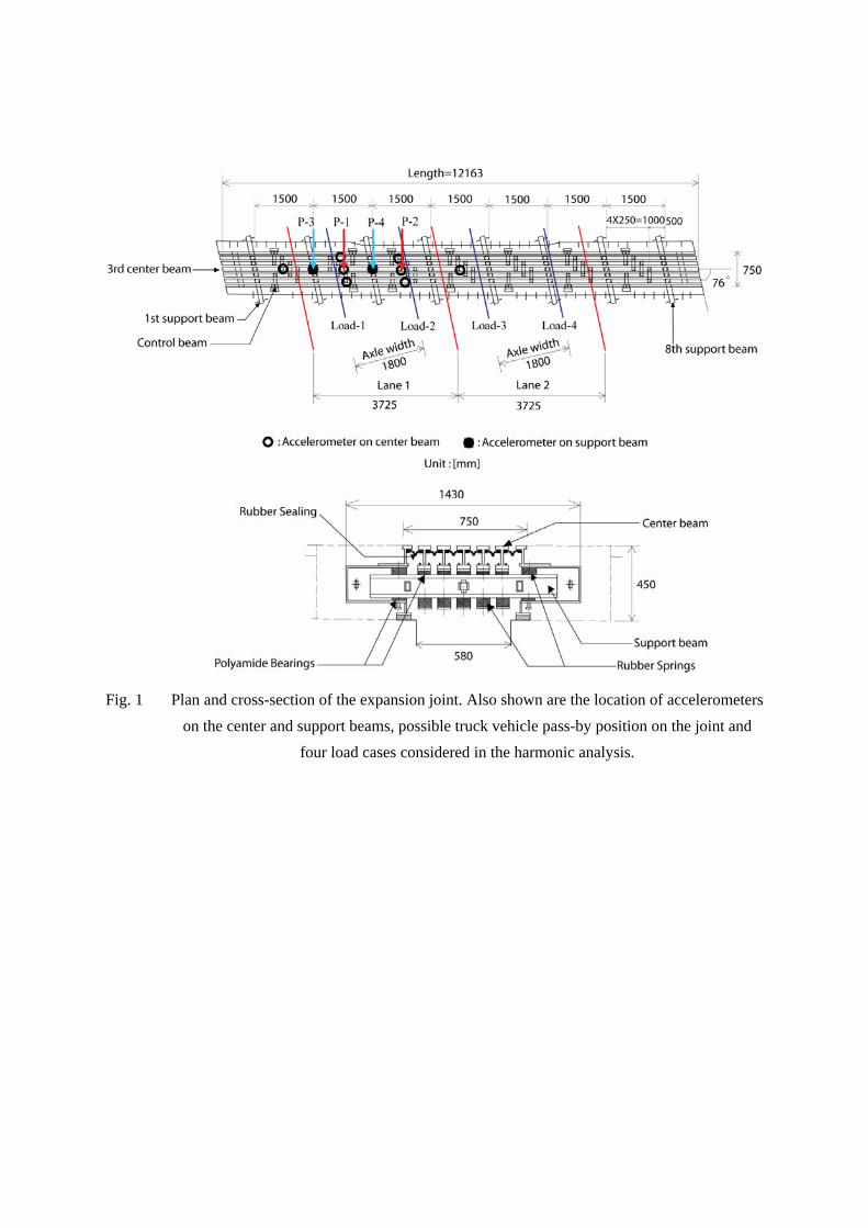
Fig. 1 Plan and cross-section of the expansion joint. Also shown are the location of accelerometers on the center and support beams, possible truck vehicle pass-by position on the joint and

four load cases considered in the harmonic analysis.

Fig. 2 Cross-sectional view of the cavity below the expansion joint

(a) (b)

Fig. 3 Cross-section size: (a) center beam and (b) support beam

Fig. 4 Application of point loads on center beam of the joint

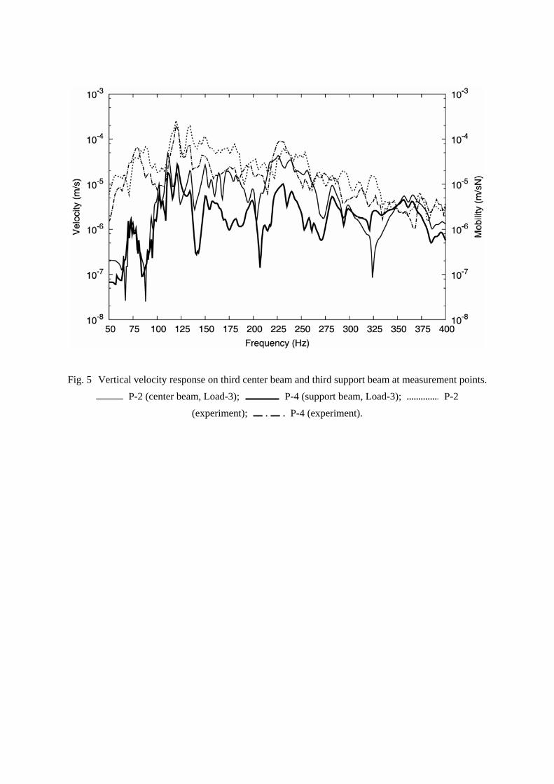
Fig. 5 Vertical velocity response on third center beam and third support beam at measurement points. P-2 (center beam, Loa P-4 (support beam, Lo P-2

P-4 (experimd-3); ad-3);

(experiment); ent).

(a) (b)

Fig. 6 Structural modes of the joint in vertical direction: (a) 110.7 Hz and (b) 356.8 Hz.

Fig. 7 Sound pressure response inside the cavity. Load-3; experiment; natural frequency of structural mode; natural frequency of acoustic mode.

Z Y

X

Fig. 8 Acoustic mode of the cavity at 106.4 Hz

Fig. 9 Radiation efficiency of the joint-cavity system. Load-1; Load-2;

Load-3; Load-4.

0 degree

12 m 24 m

48 m 96 m

Fig. 10 Sound radiation pattern at 149 Hz

96 m 48 m

24 m 12 m

Fig. 11 Sound radiation pattern at 392 Hz

Fig. 12 Changes in the sound pressure with distance from the center of the joint at 300° to Load-3.

110 Hz; 122 Hz; 149 Hz; 282 Hz; 332 Hz; 392 Hz.

80 m

-6 dB

40 m

(0,1)

(0,2) (0,3)

(0,4)

(0,5)

(1,1) (1,2)

(0,6)

(1,3) (1,4)

Fig. 13 Main lobe radiation angles of acoustic modes of the cavity.

Fig. 14 Fourier transforms of vertical velocity response of the joint at P-2 on third center beam to transient loading applied at Load-3 position (Fig. 1) corresponding to different vehicle speeds. 60 kmh-1; 80 kmh-1; 100 kmh-1.

Fig. 15 Variation of multiples of tire pulse frequency, ft, with vehicle speed. 0.8ft ;

ft; 2ft ; 3ft; 4ft; natural frequency of structural mode; natural frequency of acoustic mode.

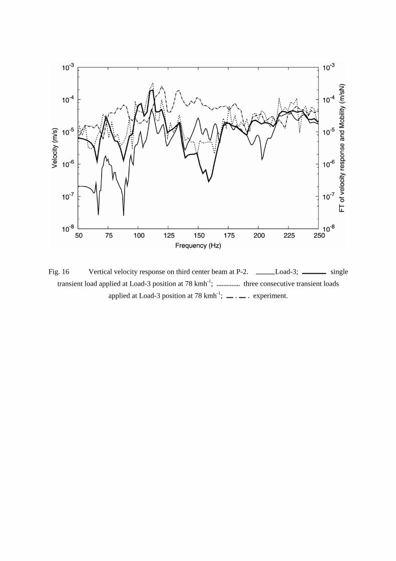
Fig. 16 Vertical velocity response on third center beam at P-2. Load-3; single transient load applied at Load-3 position at 78 kmh-1; three consecutive transient loads

applied at Load-3 position at 78 kmh-1; experiment.

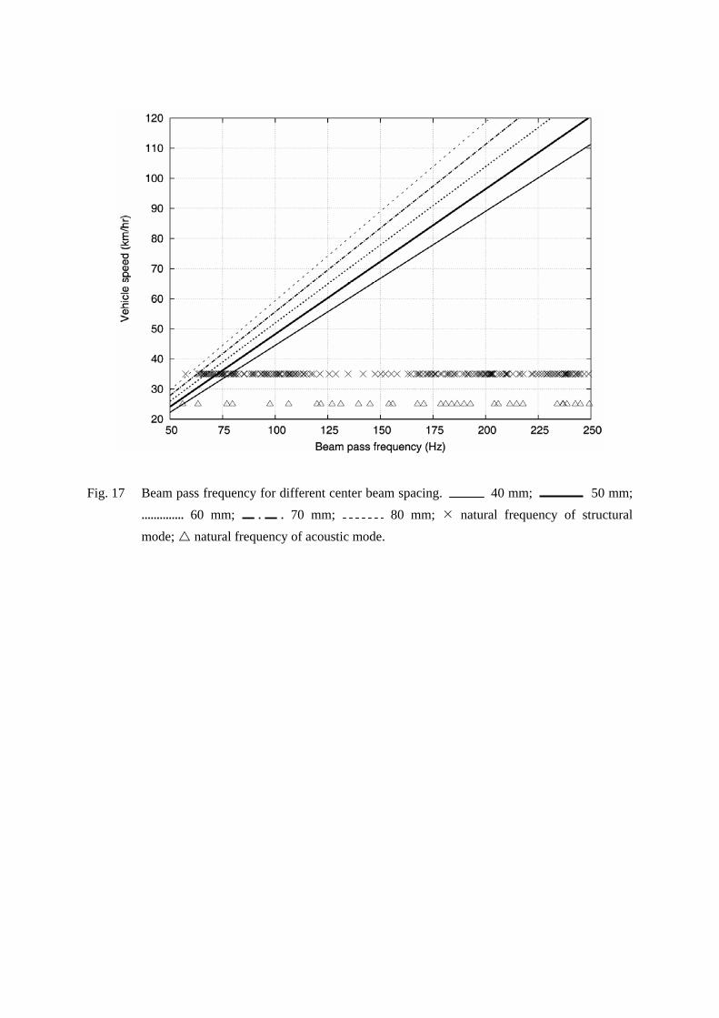
Fig. 17 Beam pass frequency for different center beam spacing. 40 mm; 50 mm; 60 mm; 70 mm; 80 mm; natural frequency of structural

mode; natural frequency of acoustic mode.

Table 1 Spring constants of bearings and springs

Center beam Support beam Control beam

Polyamide

bearing Rubber spring

Polyamide

bearing Rubber spring Control spring

Vertical (N/m) 5.67 x 108 1.50 x 106 5.97 x 108 5.83 x 106 3.52 x 105

Lateral (N/m) 2.02 x 108 5.07 x 105 0 1.97 x 106 1.19 x 105

Torsion (Nm) 3.94 x 106 9.76 x 103 0 3.89 x 104 2.32 x 103

Rotation (Nm) 2.15 x 105 5.56 x 102 0 2.27 x 103 1.34 x 102