Proceedings World Geothermal Congress 2010 Bali, Indonesia, 25-29 April 2010

1

Numerical Modeling of Complex Geothermal Steam Transportation Networks: the Cases of Cerro Prieto and Los Azufres, Mexico

Alfonso García-Gutiérrez1, J. Ignacio Martínez-Estrella1, Abel. F. Hernández-Ochoa1, Ismael Canchola-Félix2, Alfredo Mendoza-Covarrubias3

1Instituto de Investigaciones Eléctricas, Gerencia de Geotermia, Av. Reforma 113, Col. Palmira, 62490 Cuernavaca, Mor., México 2Comisión Federal de Electricidad, Residencia Cerro Prieto, Km.25 Carr. Mexicali-Pascualitos-Pescaderos, B.C., México

3Comisión Federal de Electricidad, Residencia Los Azufres, Campamento Agua Fría, Mich., México

aggarcia@iie.org.mx

Keywords: Geothermal; Steam transportation network; Numerical simulation; Hydraulic model; Pressure loss; Heat loss; Cerro Prieto; Los Azufres; Mexico

ABSTRACT

Modeling and simulation of steam flow in the transportation networks of the Cerro Prieto and Los Azufres geothermal fields, Mexico were carried out in order to determine steam pressures, temperatures, flow directions and velocities, using commercially available simulation software. For each field, a detailed hydraulic model of the pipeline network was first constructed and then each model validated by comparing simulation results with specific data measured for calibration purposes. Then, flow simulations were performed for specific dates and cases for each network. The results showed in general a good agreement between computed and measured well pressures and flow rates at the power plants inlet, with mean relative differences of less than 10%, which is considered a highly satisfactory result given the geometrical complexity and length of each geothermal field network. The low-pressure network of the CPGF showed originally larger pressure and steam flowrate differences, so that an analysis was made in order to reduce these differences and to try to explain the more likely causes of such differences. The experience from these study cases demonstrate the usefulness and suitability of numerical modeling as a tool to evaluate the overall performance of complex steam transportation systems under different operating conditions, and the feasibility of simulating large pipeline network systems reliably using state-of-the-art simulation tools.

1. INTRODUCTION

In geothermal fields, the steam from producing wells is usually transported through a network of pipelines to the power plants which may be sited several hundred meters or even some kilometers away. The network geometry becomes rather complicated and this fact quite difficult to predict the pressure or flow rates changes due to the normal operation of the transportation network or due to specific events like the opening or closing of valves; the integration of new wells; shut-down of existing wells, and start-up or shut down of power plants without a numerical tool. Therefore, numerical modeling and simulation of the steam transportation network constitutes an essential tool to evaluate the operating conditions (pressure, temperature and flow rate) at almost any position in the network; information which otherwise is very difficult to obtain experimentally since steam pipelines are regarded as high-pressure vessels.

Marconcini and Neri (1979) pioneered work on geothermal steam pipeline network simulation. They developed the VAPSTAT-1 computer code and simulated a six-well steam pipeline network of the type used at Larderello, Italy. Huang (1990) and Huang and Freeston (1992; 1993) developed a model of steam supply and reinjection pipeline network which was applied to the simulation of the Ohaki and Larderello geothermal fields, and to the study pipe of roughness effects in a reinjection network. Bettagli and Bidini (1996) carried out an energy-exergy study of a 32-well and three-turbine system of the Larderello-Valle Secolo-Farinello geothermal area. DiMaria (2000) developed the PowerPipe numerical code and analyzed the pipe network of a geothermal power plant under design and off-design conditions.

Regarding the Mexican geothermal fields, Sánchez et al. (1987) developed a homogeneous drift-model for sizing pipelines with elevation changes and tested it in Los Azufres, Mexico. Peña (1986) and Peña and Campbell (1988) derived a model based on the polytropic expansion of steam and determined the energy losses in a horizontal network at Cerro Prieto. Cruickshank et al. (1990) developed an adiabatic model of steam flow for the Cerro Prieto pipeline network. However, these models were not tested extensively and their real applicability is unknown. In the last few years, two extensive studies were performed by García-Gutiérrez et al. (2006; 2008; 2009), in which they developed detailed hydraulic models and simulated the steam flow in the transportation networks of the Cerro Prieto and Los Azufres geothermal fields, respectively, using commercially available simulation software.

This paper is based on the results obtained from the last two studies aforementioned. Simulation results are presented and analyzed on the behavior of each field-wide pipeline network for specific dates. A brief description on the methodology for documentating the numerical models is also included.

2. DESCRIPTION OF THE CERRO PRIETO AND LOS AZUFRES STEAM TRANSPORTATION NETWORKS

2.1 Cerro Prieto Pipeline Network

The Cerro Prieto geothermal field (CPGF) is one of the largest liquid dominant geothermal fields in the world and its present installed capacity is 720 MWe. It is composed of four field areas named progressively from Cerro Prieto One (CP1) to Cerro Prieto Four (CP4). The installed power plants are of the condensing type and include four-37.5MWe units and one-30MWe unit in CP1; two-

García-Gutiérrez et al.

2

110MWe units in CP2 and in CP3, and four-25MWe units in CP4 (Gutiérrez-Negrín and Quijano-León, 2005).

The Cerro Prieto pipe network is essentially of the distributed system type (Huang, 1990) where most of the separators are located immediately adjacent to each production well and individual pipelines transport steam to the main collecting ducts, called branches. The network is composed essentially by a set of pipes over a rather flat terrain however its multiple interconnections and different arrangements for steam separation make it rather complex.. CP1 has high-pressure steam separation only whereas CP2, CP3 and CP4 have both high- and low-pressure separation. In CP4 there are “separation islands” which are squared areas 125 x 125 m, subdivided into four modules. Each module has four high-pressure separators, each receiving the two-phase flow from a well. Then, the separated water of the four streams is mixed and fed to a single separator to obtain low-pressure steam. Most of the separated water is finally sent to the evaporative pond via open channels, although some water is re-injected back into the reservoir.

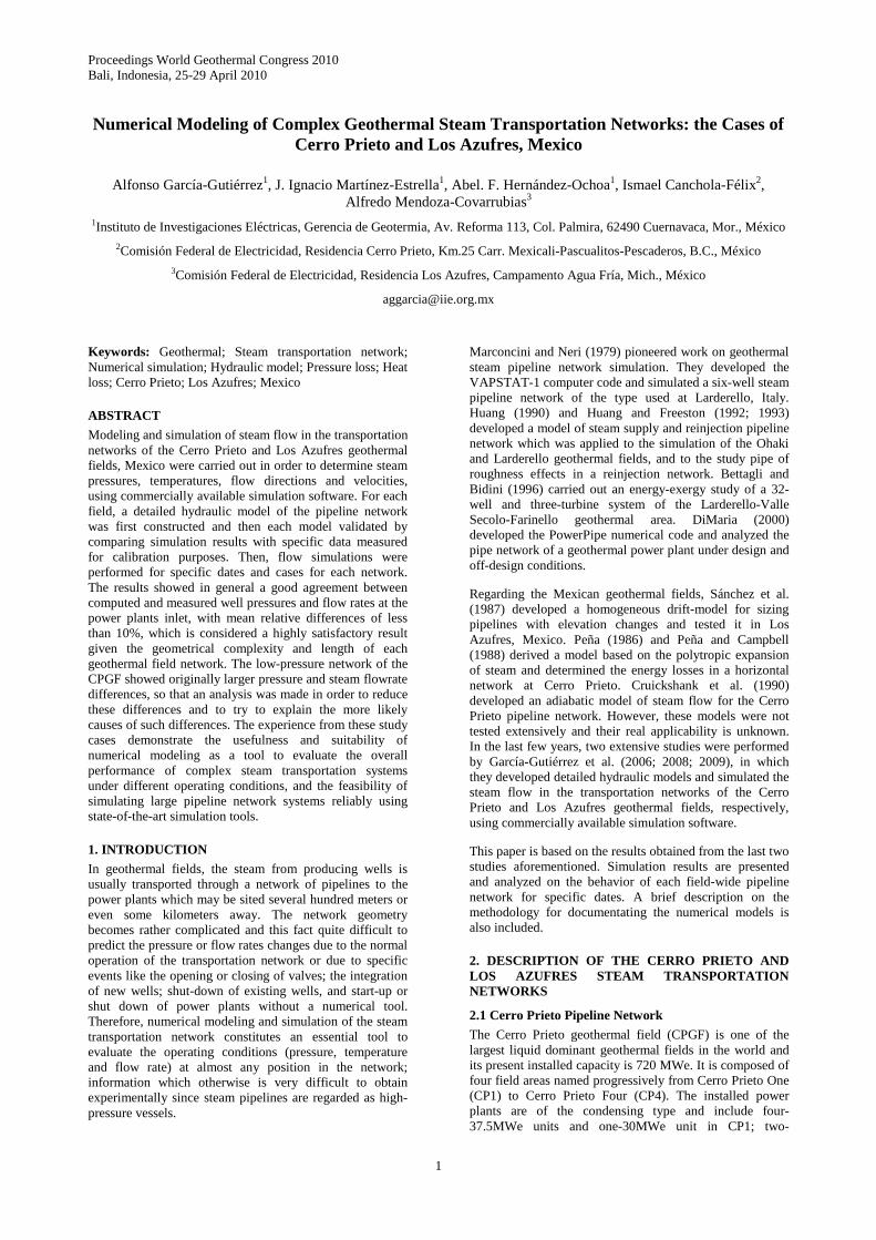
The separated steam is transported to the power plants in a pipeline network 125 km long approximately, with high- and low-pressure pipelines running parallel. The pipe diameters range from 8” to 46”. They are thermally insulated with mineral wool or glass fiber and an exterior layer of aluminum or wrought iron. The network has 183 connected wells of which 162 are producing wells, the rest being wells for future integration; yet, a single branch may collect the steam from 1 to 36 wells. These branches feed steam to the power plants. The network has several interconnections among wells and pipelines that allow for an adequate steam supply to the power plants by sending steam in different directions to specific points on the network. Figure 1 shows the CPGF transportation network.

2.1 Los Azufres Pipeline Network

The Los Azufres geothermal field (LAGF) is located in the central part of Mexico, in the physiographic province of the Mexican Volcanic Belt. It is situated in a mountainous range with elevations ranging from 2800 to 3000 m.a.s.l. The field is divided into two well-defined zones: Maritaro in the North and Tejamaniles in the South, with a separation of a few kilometers between them.

Presently there are 14 power plants in the field with a total installed capacity of 188 MWe. The plants include one-50 MWe; four-25 MWe single-flash units, seven-5 MWe wellhead (back-pressure) units, and two-1.5 MWe binary units. The installed capacity of the North and South zones is 95 MWe and 93 MWe, respectively. Seven units are installed in each zone.

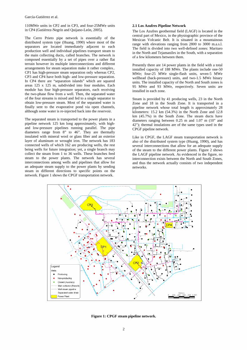
Steam is provided by 41 producing wells, 23 in the North Zone and 18 in the South Zone. It is transported in a pipeline network whose total length is approximately 28 kilometers: 15.2 km (54.3%) in the North Zone and 12.8 km (45.7%) in the South Zone. The steam ducts have diameters ranging between 0.25 m and 1.07 m (10" and 42"); thermal insulations are of the same types used in the CPGF pipeline network.

Like in CPGF, the LAGF steam transportation network is also of the distributed system type (Huang, 1990), and has several interconnections that allow for an adequate supply of the steam to the different power plants. Figure 2 shows the LAGF pipeline network. As evidenced in the figure, no interconnection exists between the North and South Zones, and thus the network actually consists of two independent networks.

Figure 1: CPGF steam pipeline network.

García-Gutiérrez et al.

3

Figure 2: LAGF steam pipeline network.

3. METHODOLOGY

3.1 Data Gathering and Documentation of the Hydraulic Models

The development of both CPGF and LAGF steam transportation network models followed a similar procedure. It began with the gathering of design and construction information related to each pipeline network such as drawings, diagrams, and other available field sources of information, such as topographical maps and digital aerial photographs, etc. Primary data for building the models included pipe geometric characteristics and materials, insulating materials, fittings, etc. Field visits were made whenever missing or obsolete information was found, a task that was complicated due to the geometrical complexity of the networks and, in the case of LAGF, by its topographical and dense vegetation characteristics.

When needed, MS Excel spreadsheets were used to carry out automated trigonometric calculations in order to build the plant and elevation profiles of each pipeline. Input data for the numerical simulator were obtained from these profiles, such as the actual length of pipe segments, elevation differences and angles of elbows and bends, etc. This was particularly detailed for the LAGF steam transportation network.

This process allowed definition of the structure of each network model through the identification of all existing interconnection nodes and the segments of each pipeline between nodes, as well as the sequence of all flow components (pipes, fittings, valves, elbows, etc.) that are

connected in each network pipeline. Additionally, a specific nomenclature was developed in order to identify each network pipeline and to facilitate handling of the enormous amount of network data.

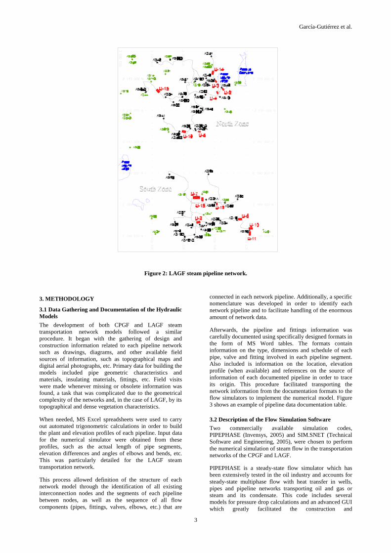
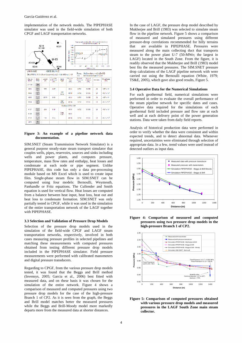
Afterwards, the pipeline and fittings information was carefully documented using specifically designed formats in the form of MS Word tables. The formats contain information on the type, dimensions and schedule of each pipe, valve and fitting involved in each pipeline segment. Also included is information on the location, elevation profile (when available) and references on the source of information of each documented pipeline in order to trace its origin. This procedure facilitated transporting the network information from the documentation formats to the flow simulators to implement the numerical model. Figure 3 shows an example of pipeline data documentation table.

3.2 Description of the Flow Simulation Software

Two commercially available simulation codes, PIPEPHASE (Invensys, 2005) and SIM.SNET (Technical Software and Engineering, 2005), were chosen to perform the numerical simulation of steam flow in the transportation networks of the CPGF and LAGF.

PIPEPHASE is a steady-state flow simulator which has been extensively tested in the oil industry and accounts for steady-state multiphase flow with heat transfer in wells, pipes and pipeline networks transporting oil and gas or steam and its condensate. This code includes several models for pressure drop calculations and an advanced GUI which greatly facilitated the construction and

García-Gutiérrez et al.

4

implementation of the network models. The PIPEPHASE simulator was used in the field-wide simulation of both CPGF and LAGF transportation networks.

Figure 3: An example of a pipeline network data documentation.

SIM.SNET (Steam Transmission Network Simulator) is a general purpose steady-state steam transport simulator that couples wells, pipes, reservoirs, sources and sinks including wells and power plants, and computes pressure, temperature, mass flow rates and enthalpy, heat losses and condensate at each node or pipe segment. Unlike PIPEPHASE, this code has only a data pre-processing module based on MS Excel which is used to create input files. Single-phase steam flow in SIM.SNET can be computed using four models: Bernoulli, Weymouth, Panhandle or Fritz equations. The Cullender and Smith equation is used for vertical flow. Heat losses are computed from a balance between heat input, heat loss, heat out and heat loss to condensate formation. SIM.SNET was only partially tested in CPGF, while it was used in the simulation of the entire transportation network of the LAGF together with PIPEPHASE.

3.3 Selection and Validation of Pressure Drop Models

Selection of the pressure drop models used in the simulation of the field-wide CPGF and LAGF steam transportation networks, respectively, involved in both cases measuring pressure profiles in selected pipelines and matching these measurements with computed pressures obtained from testing different pressure drop models included in the PIPEPHASE simulator. Field pressure measurements were performed with calibrated manometers and digital pressure transducers.

Regarding to CPGF, from the various pressure drop models tested, it was found that the Beggs and Brill method (Invensys, 2005; Garcia et al., 2006) best fitted with measured data, and on these basis it was chosen for the simulation of the entire network. Figure 4 shows a comparison of measured and computed pressures using two pressure drop models for the case of the high-pressure Branch 1 of CP2. As it is seen from the graph, the Beggs and Brill model matches better the measured pressures while the Beggs and Brill-Moody model more markedly departs more from the measured data at shorter distances.

In the case of LAGF, the pressure drop model described by Mukherjee and Brill (1983) was selected to simulate steam flow in the pipeline network. Figure 5 shows a comparison of measured and simulated pressures using different pressure-drop correlations recommended for hilly terrains that are available in PIPEPHASE. Pressures were measured along the main collecting duct that transports steam to the power plant U-7 (50-MWe; the largest in LAGF) located in the South Zone. From the figure, it is readily observed that the Mukherjee and Brill (1983) model best fits the measured pressures. The SIM.SNET pressure drop calculations of the LAGF pipeline network with were carried out using the Bernoulli equation (White, 1979; TS&E, 2005), which gave also good results, Figure 5.

3.4 Operative Data for the Numerical Simulations

For each geothermal field, numerical simulations were performed in order to evaluate the overall performance of the steam pipeline network for specific dates and cases. Operative data required for the simulations of each geothermal field included pressure and flow rate at each well and at each delivery point of the power generation stations. Data were taken from daily field reports.

Analysis of historical production data were performed in order to verify whether the data were consistent and within expected trends, and to detect abnormal data. Whenever required, uncertainties were eliminated through selection of appropriate data. In a few, trend values were used instead of detected outliers as input data.

1.20

1.25

1.30

1.35

1.40

1.45

1.50

1.55

1.60

0 200 400 600 800 1000 1200 1400

Pre

ssu

re (M

Pa)

Distance (m)

Measured data with pressure transducer

Measured pressure with manometers

Simulation PIPEPHASE - Beggs & Brill-Moody

Simulation PIPEPHASE - Beggs & Brill

Figure 4: Comparison of measured and computed pressures using two pressure drop models in the high-pressure Branch 1 of CP2.

0.92

0.94

0.96

0.98

1.00

1.02

1.04

1.06

0 200 400 600 800 1000 1200 1400

Pre

ssu

re (M

Pa)

Distance (m)

Measured with manometer

Measured with pressure transducer

Simulation PIPEPHASE - Mukherjee & Brill

Simulation PIPEPHASE - Beggs & Brill

Simulation PIPEPHASE - Beggs & Brill - Moody

Simulation SIM.SNET - Bernoulli

Fixed Pressure in U-7 = 0.956 MPaFixed Flowrate in U-13 = 190 t/hFixed Flowrate at

well Az-06 = 56.6

Butterfly valve Nominal diameter 1.07 m (42")

Aperture = 70%

Figure 5: Comparison of computed pressures obtained with various pressure drop models and measured pressures in the LAGF South Zone main steam collector.

García-Gutiérrez et al.

5

4. SIMULATION RESULTS AND DISCUSSION

4.1 Simulation Results of the Cerro Prieto Pipeline Network

As described previously, the CPGF steam pipeline network is a large and complex system which includes high- and low-pressure steam ducts running in parallel, although primary and secondary separated steam typically do not mix during their transport to the delivery points of the power plants. This allowed modeling the steam transportation system as two independent networks rather than a single system. Simulation results of the CPGF are then presented for both the high- and low-pressure pipeline networks.

4.1.1 Cerro Prieto high-pressure pipeline network

Once the high-pressure pipeline network model was set-up in the PIPEPHASE simulator according to the operative information of the selected date for simulation, it was observed that the model was further subdivided into two submodels, one including mostly wells from the CP3 and CP4 field areas, and the other grouping wells from the CP1 and CP2 field areas.

These two submodels or “blocks” were connected only through a pipeline running between the CP2 and CP3 field areas, which had installed a bypass equipped with a 12” butterfly valve opened at 5% of full aperture. Given this

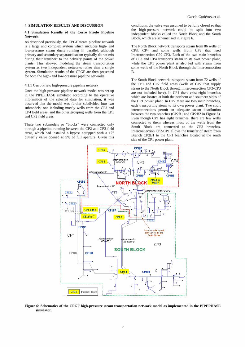
conditions, the valve was assumed to be fully closed so that the high-pressure network could be split into two independent blocks called the North Block and the South Block, which are schematized in Figure 6.

The North Block network transports steam from 86 wells of CP3, CP4 and some wells from CP2 that feed Interconnection CP2-CP3. Each of the two main branches of CP3 and CP4 transports steam to its own power plant, while the CP1 power plant is also fed with steam from some wells of the North Block through the Interconnection B.

The South Block network transports steam from 72 wells of the CP1 and CP2 field areas (wells of CP2 that supply steam to the North Block through Interconnection CP2-CP3 are not included here). In CP1 there exist eight branches which are located at both the northern and southern sides of the CP1 power plant. In CP2 there are two main branches, each transporting steam to its own power plant. Two short interconnections permit an adequate steam distribution between the two branches (CP2B1 and CP2B2 in Figure 6). Even though CP1 has eight branches, there are few wells connected to them whereas most of the wells from the South Block are connected to the CP2 branches. Interconnection CP2-CP1 allows the transfer of steam from Branch CP2B1 to the CP1 branches located at the south side of the CP1 power plant.

Figure 6: Schematics of the CPGF high-pressure steam transportation network model as implemented in the PIPEPHASE simulator.

García-Gutiérrez et al.

6

For the simulations of the CPGF high-pressure pipeline network, each well was considered as a source boundary condition since flow rate at the orifice plate of each well is known. Similarly, pressures at the inlet of each power plant were originally fixed as sink boundary conditions. However, under this scheme, numerical instability and convergence problems arose, and thus some of the sinks were modeled with flow rate as boundary condition (see Tables 1 and 2).

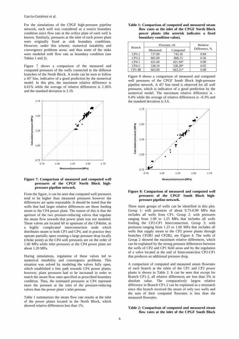
Figure 7 shows a comparison of the measured and computed pressures of the wells connected to the different branches of the North Block. A tredn can be seen to follow a 45º line, indicative of a good prediction by the numerical model. In this plot, the maximum relative difference is 6.61% while the average of relative differences is 2.36% and the standard deviation is 2.19.

0.75

1.00

1.25

1.50

1.75

0.75 1.00 1.25 1.50 1.75

Cal

cula

ted

pre

ssu

re (M

Pa)

Measured pressure (MPa)

Figure 7: Comparison of measured and computed well pressures of the CPGF North Block high-pressure pipeline network.

From the figure, it can be seen that computed well pressures tend to be higher than measured pressures however the differences are quite reasonable. It should be noted that the wells that had larger relative differences are those feeding steam to the CP4 power plant. The reason of this is that the aperture of the two pressure-reducing valves that regulate the steam flow towards that power plant was not modeled. These valves are located 60 m upstream of the CP4inlet, in a highly complicated interconnection node which distributes steam to both CP3 and CP4, and in practice they operate partially open creating a large pressure drop locally (choke point) as the CP4 well pressures are on the order of 1.60 MPa while inlet pressures at the CP4 power plant are about 1.20 MPa.

During simulations, regulation of these valves led to numerical instability and convergence problems. This situation was solved by modeling the valves fully open, which established a free path towards CP4 power plants; however, plant pressures had to be increased in order to match the steam flow rates specified as prescribed boundary condition. Thus, the estimated pressures at CP4 represent more the pressure at the inlet of the pressure-reducing valves than the power plant´s inlet pressue.

Table 1 summarizes the steam flow rate results at the inlet of the power plants located in the North Block, which showed relative differences less than 1%.

Table 1: Comparison of computed and measured steam flow rates at the inlet of the CPGF North Block power plants (the asterisk indicates a fixed boundary condition value).

Flowrate, t/h Branch

Measured Computed

Relative Difference, %

CP3-1 737.00 743.18 0.84 CP3-2 865.00 868.15 0.36 CP4-1 421.60 421.94* 0.08 CP4-2 338.10 338.28* 0.05 CP1-IB 663.00 663.51* 0.08

Figure 8 shows a comparison of measured and computed well pressures of the CPGF South Block high-pressure pipeline network. A 45º line trend is observed for all well pressures, which is indicative of a good prediction by the numerical model. The maximum relative difference is -0.4% while the average of relative differences is –0.3% and the standard deviation is 3.6.

0.75

1.00

1.25

1.50

1.75

0.75 1.00 1.25 1.50 1.75

Cal

cula

ted

pre

ssu

re (M

Pa)

Measured pressure (MPa)

Figure 8: Comparison of measured and computed well pressures of the CPGF South Block high-pressure pipeline network.

Three main groups of wells can be identified in this plot. Group 1: with pressures of about 0.75-0.90 MPa that includes all wells from CP1. Group 2: with pressures ranging from 1.00 to 1.25 MPa that includes all wells feeding the CP2-CP1 Interconnection. Group 3: with pressures ranging from 1.25 to 1.60 MPa that includes all wells that supply steam to the CP2 power plants through branches CP2B1 and CP2B2, see Figure 4. The wells of Group 2 showed the maximum relative differences, which can be explained by the strong pressure differences between the wells of CP2 and CP1 field areas and by the regulation of a valve located at the end of Interconnection CP2-CP1 that produces an additional pressure drop.

A comparison of computed and measured steam flowrates of each branch at the inlets of the CP1 and CP2 power plants is shown in Table 2. It can be seen that except for Branch CP1-2, all relative differences are less than 5% in absolute value. The comparatively largest relative difference in Branch CP1-2 can be explained as a mismatch since this branch received the steam of only two wells and the sum of their computed flowrates is less than the measured flowrates.

Table 2: Comparison of computed and measured steam flow rates at the inlet of the CPGF South Block

García-Gutiérrez et al.

7

power plants (the asterisk indicates a fixed boundary condition value).

Flowrate, t/h Branch

Measured Computed

Relative Difference, %

CP1-1 58.71 61.47 4.69 CP1-2 34.79 31.85 -8.46 CP1-3 21.29 20.55 -3.48 CP1-5 187.99 195.91 4.21 CP1-6 197.67 205.29 3.86 CP1-7 244.00* 243.41 -0.24 CP2-1 794.00 774.72 -2.43 CP2-2 754.00* 748.23 -0.76

4.1.2 Cerro Prieto low-pressure pipeline network

The low-pressure steam transportation network of the CPGF is fed with the steam from the secondary separation of 77 producing wells of CP2, CP3 and CP4 field areas. No wells from CP1 field area supply steam to the low-pressure steam pipeline network.

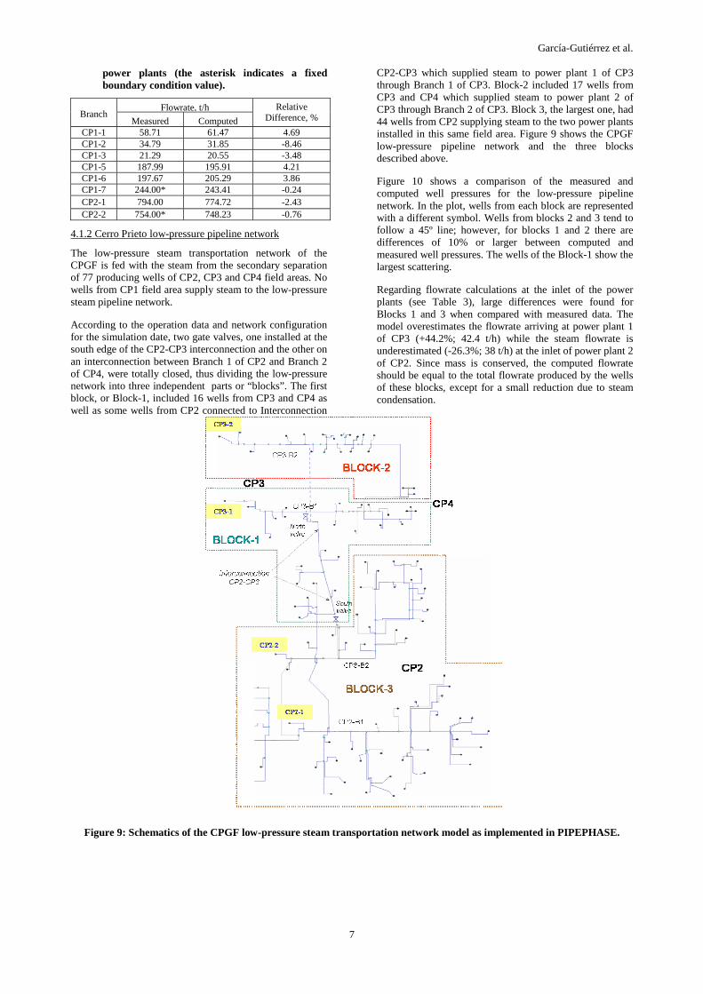
According to the operation data and network configuration for the simulation date, two gate valves, one installed at the south edge of the CP2-CP3 interconnection and the other on an interconnection between Branch 1 of CP2 and Branch 2 of CP4, were totally closed, thus dividing the low-pressure network into three independent parts or “blocks”. The first block, or Block-1, included 16 wells from CP3 and CP4 as well as some wells from CP2 connected to Interconnection

CP2-CP3 which supplied steam to power plant 1 of CP3 through Branch 1 of CP3. Block-2 included 17 wells from CP3 and CP4 which supplied steam to power plant 2 of CP3 through Branch 2 of CP3. Block 3, the largest one, had 44 wells from CP2 supplying steam to the two power plants installed in this same field area. Figure 9 shows the CPGF low-pressure pipeline network and the three blocks described above.

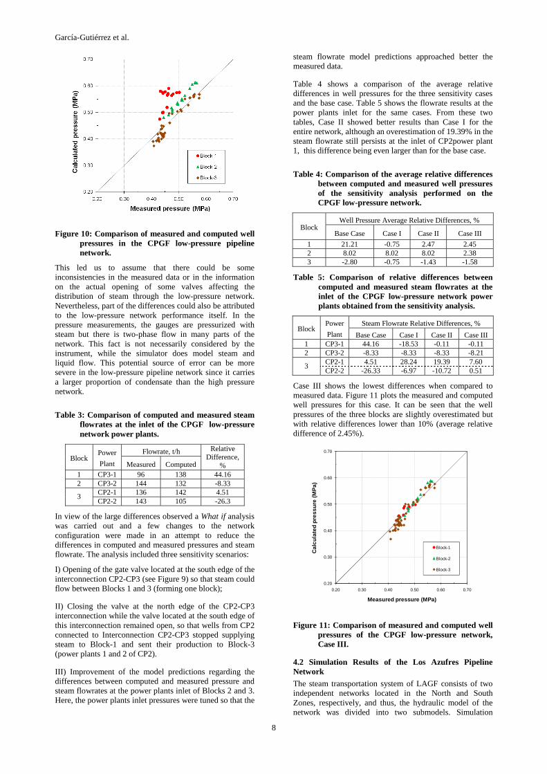
Figure 10 shows a comparison of the measured and computed well pressures for the low-pressure pipeline network. In the plot, wells from each block are represented with a different symbol. Wells from blocks 2 and 3 tend to follow a 45º line; however, for blocks 1 and 2 there are differences of 10% or larger between computed and measured well pressures. The wells of the Block-1 show the largest scattering.

Regarding flowrate calculations at the inlet of the power plants (see Table 3), large differences were found for Blocks 1 and 3 when compared with measured data. The model overestimates the flowrate arriving at power plant 1 of CP3 (+44.2%; 42.4 t/h) while the steam flowrate is underestimated (-26.3%; 38 t/h) at the inlet of power plant 2 of CP2. Since mass is conserved, the computed flowrate should be equal to the total flowrate produced by the wells of these blocks, except for a small reduction due to steam condensation.

Figure 9: Schematics of the CPGF low-pressure steam transportation network model as implemented in PIPEPHASE.

García-Gutiérrez et al.

8

Figure 10: Comparison of measured and computed well pressures in the CPGF low-pressure pipeline network.

This led us to assume that there could be some inconsistencies in the measured data or in the information on the actual opening of some valves affecting the distribution of steam through the low-pressure network. Nevertheless, part of the differences could also be attributed to the low-pressure network performance itself. In the pressure measurements, the gauges are pressurized with steam but there is two-phase flow in many parts of the network. This fact is not necessarily considered by the instrument, while the simulator does model steam and liquid flow. This potential source of error can be more severe in the low-pressure pipeline network since it carries a larger proportion of condensate than the high pressure network.

Table 3: Comparison of computed and measured steam flowrates at the inlet of the CPGF low-pressure network power plants.

Flowrate, t/h Block

Power

Plant Measured Computed

Relative Difference,

% 1 CP3-1 96 138 44.16 2 CP3-2 144 132 -8.33

CP2-1 136 142 4.51 3

CP2-2 143 105 -26.3

In view of the large differences observed a What if analysis was carried out and a few changes to the network configuration were made in an attempt to reduce the differences in computed and measured pressures and steam flowrate. The analysis included three sensitivity scenarios:

I) Opening of the gate valve located at the south edge of the interconnection CP2-CP3 (see Figure 9) so that steam could flow between Blocks 1 and 3 (forming one block);

II) Closing the valve at the north edge of the CP2-CP3 interconnection while the valve located at the south edge of this interconnection remained open, so that wells from CP2 connected to Interconnection CP2-CP3 stopped supplying steam to Block-1 and sent their production to Block-3 (power plants 1 and 2 of CP2).

III) Improvement of the model predictions regarding the differences between computed and measured pressure and steam flowrates at the power plants inlet of Blocks 2 and 3. Here, the power plants inlet pressures were tuned so that the

steam flowrate model predictions approached better the measured data.

Table 4 shows a comparison of the average relative differences in well pressures for the three sensitivity cases and the base case. Table 5 shows the flowrate results at the power plants inlet for the same cases. From these two tables, Case II showed better results than Case I for the entire network, although an overestimation of 19.39% in the steam flowrate still persists at the inlet of CP2power plant 1, this difference being even larger than for the base case.

Table 4: Comparison of the average relative differences between computed and measured well pressures of the sensitivity analysis performed on the CPGF low-pressure network.

Well Pressure Average Relative Differences, % Block

Base Case Case I Case II Case III

1 21.21 -0.75 2.47 2.45 2 8.02 8.02 8.02 2.38 3 -2.80 -0.75 -1.43 -1.58

Table 5: Comparison of relative differences between computed and measured steam flowrates at the inlet of the CPGF low-pressure network power plants obtained from the sensitivity analysis.

Steam Flowrate Relative Differences, % Block

Power

Plant Base Case Case I Case II Case III 1 CP3-1 44.16 -18.53 -0.11 -0.11 2 CP3-2 -8.33 -8.33 -8.33 -8.21

CP2-1 4.51 28.24 19.39 7.60 3

CP2-2 -26.33 -6.97 -10.72 0.51

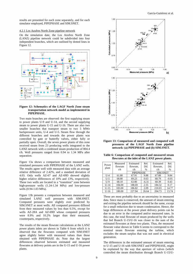
Case III shows the lowest differences when compared to measured data. Figure 11 plots the measured and computed well pressures for this case. It can be seen that the well pressures of the three blocks are slightly overestimated but with relative differences lower than 10% (average relative difference of 2.45%).

0.20

0.30

0.40

0.50

0.60

0.70

0.20 0.30 0.40 0.50 0.60 0.70

Cal

cula

ted

pre

ssu

re (

MP

a)

Measured pressure (MPa)

Block-1

Block-2

Block-3

Figure 11: Comparison of measured and computed well pressures of the CPGF low-pressure network, Case III.

4.2 Simulation Results of the Los Azufres Pipeline Network

The steam transportation system of LAGF consists of two independent networks located in the North and South Zones, respectively, and thus, the hydraulic model of the network was divided into two submodels. Simulation

García-Gutiérrez et al.

9

results are presented for each zone separately, and for each simulator employed, PIPEPHASE and SIM.SNET.

4.2.1 Los Azufres North Zone pipeline network

On the simulation date, the Los Azufres North Zone (LANZ) pipeline network could be subdivided into four independent branches, which are outlined by dotted lines in Figure 12.

Figure 12: Schematics of the LAGF North Zone steam transportation network model as implemented in PIPEPHASE.

Two main branches are observed: the first supplying steam to power plants U-9 and U-14, and the second supplying steam to power plants U-15 and U-16. There are also two smaller branches that transport steam to two 5 MWe backpressure units, U-4 and U-5. Steam flow through the different branches and towards the power plants was controlled by gate or butterfly valves, either fully or partially open. Overall, the seven power plants of this zone received steam from 23 producing wells integrated to the LANZ network with a combined steam production of 804.4 t/h. Well pressures ranged from 0.94 to 1.34 MPa after separation.

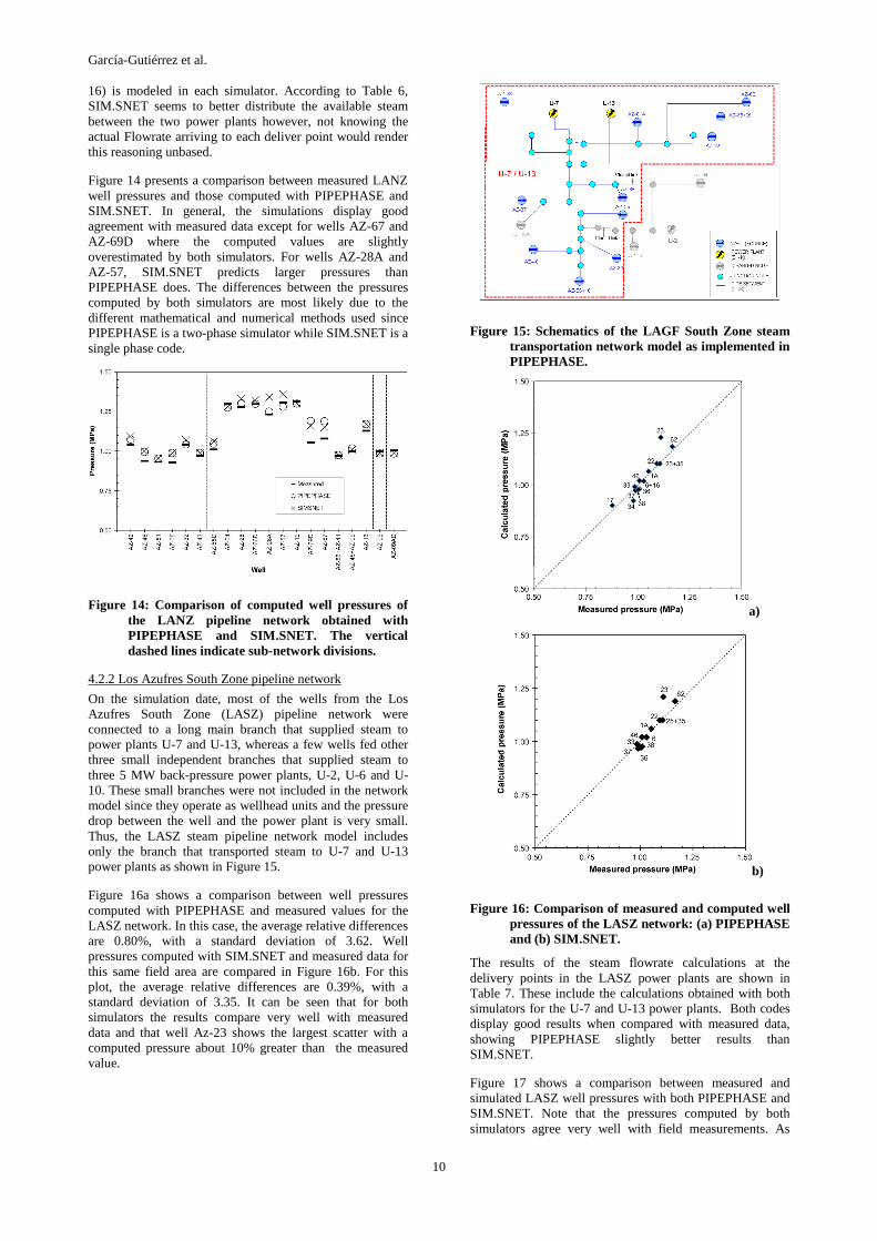
Figure 13a shows a comparison between measured and simulated pressures with PIPEPHASE of the LANZ wells. The results agree well with measured data with an average relative difference of 2.42%, and a standard deviation of 4.03. Only wells AZ-67 and AZ-69D showed slightly higher relative differences of 10% and 13%, respectively. These two wells are located in a “transition” zone between high-pressure wells (1.24-1.34 MPa) and low-pressure wells (0.94-1.03 MPa).

Figure 13b presents a comparison between measured and simulated LANZ well pressures with SIM.SNET. Computed pressures were slightly over predicted by SIM.SNET at most wells. All computed pressures differed from their measured values by less than 6.5%, except for wells AZ-28A and AZ-69D whose computed pressures were 8.9% and 10.2% larger than their measured, counterparts, respectively.

The results of the steam flowrate calculations at the LANZ power plants inlets are shown in Table 6 from which it is observed that the flowrates computed with SIM.SNET agree slightly better with measured values than those obtained with PIPEPHASE do. Note that the largest differences observed between estimated and measured flowrates at delivery points are in the U-15 and U-16 power plants.

a)

b)

Figure 13: Comparison of measured and computed well pressures of the LAGF North Zone pipeline network: (a) PIPEPHASE and (b) SIM.SNET.

Table 6: Comparison of computed and measured steam flowrates at the inlet of the LANZ power plants.

Estimated flowrate,

t/h

Rel. Dif. %

Estimated flowrate,

t/h

Rel. Dif. %

Power plant

Measured flowrate

t/h PIPEPHASE SIM.SNET

U-4 61.80 67.91 9.88 67.88 9.84 U-5 68.80 69.23 0.63 68.79 -0.01 U-9 68.10 63.80 -6.31 68.39 0.43

U-14 184.00 188.69 2.55 184.32 0.17 U-15 183.00 186.82 2.09 210.03 14.77 U-16 180.00 227.94 26.64 204.73 13.74

These are most probably due to an uncertainty in measured data. Since mass is conserved, the amount of steam entering and exiting the pipeline network should be the same, except for a small reduction due to steam condensation. Hence, the large differences at the power plant delivery points can be due to an error in the computed and/or measured rates. In this case, the total flowrate of steam produced by the wells that fed Branch U-15/U-16 was closer to the sum of the estimated flowrates at these two plants. Thus, the measured flowrate value shown in Table 6 seems to correspond to the nominal steam flowrate entering the turbine, which excludes the steam surplus that was not used in electrical generation.

The differences in the estimated amount of steam entering to U-15 and U-16 with SIM.SNET and PIPEPHASE, might be explained by the way that aperture of valves (which controlled the steam distribution through Branch U-15/U-

García-Gutiérrez et al.

10

16) is modeled in each simulator. According to Table 6, SIM.SNET seems to better distribute the available steam between the two power plants however, not knowing the actual Flowrate arriving to each deliver point would render this reasoning unbased.

Figure 14 presents a comparison between measured LANZ well pressures and those computed with PIPEPHASE and SIM.SNET. In general, the simulations display good agreement with measured data except for wells AZ-67 and AZ-69D where the computed values are slightly overestimated by both simulators. For wells AZ-28A and AZ-57, SIM.SNET predicts larger pressures than PIPEPHASE does. The differences between the pressures computed by both simulators are most likely due to the different mathematical and numerical methods used since PIPEPHASE is a two-phase simulator while SIM.SNET is a single phase code.

Figure 14: Comparison of computed well pressures of the LANZ pipeline network obtained with PIPEPHASE and SIM.SNET. The vertical dashed lines indicate sub-network divisions.

4.2.2 Los Azufres South Zone pipeline network

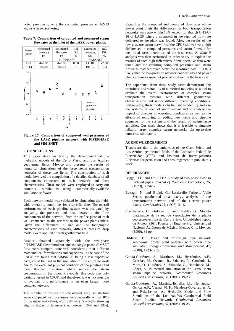
On the simulation date, most of the wells from the Los Azufres South Zone (LASZ) pipeline network were connected to a long main branch that supplied steam to power plants U-7 and U-13, whereas a few wells fed other three small independent branches that supplied steam to three 5 MW back-pressure power plants, U-2, U-6 and U-10. These small branches were not included in the network model since they operate as wellhead units and the pressure drop between the well and the power plant is very small. Thus, the LASZ steam pipeline network model includes only the branch that transported steam to U-7 and U-13 power plants as shown in Figure 15.

Figure 16a shows a comparison between well pressures computed with PIPEPHASE and measured values for the LASZ network. In this case, the average relative differences are 0.80%, with a standard deviation of 3.62. Well pressures computed with SIM.SNET and measured data for this same field area are compared in Figure 16b. For this plot, the average relative differences are 0.39%, with a standard deviation of 3.35. It can be seen that for both simulators the results compare very well with measured data and that well Az-23 shows the largest scatter with a computed pressure about 10% greater than the measured value.

Figure 15: Schematics of the LAGF South Zone steam transportation network model as implemented in PIPEPHASE.

a)

b)

Figure 16: Comparison of measured and computed well pressures of the LASZ network: (a) PIPEPHASE and (b) SIM.SNET.

The results of the steam flowrate calculations at the delivery points in the LASZ power plants are shown in Table 7. These include the calculations obtained with both simulators for the U-7 and U-13 power plants. Both codes display good results when compared with measured data, showing PIPEPHASE slightly better results than SIM.SNET.

Figure 17 shows a comparison between measured and simulated LASZ well pressures with both PIPEPHASE and SIM.SNET. Note that the pressures computed by both simulators agree very well with field measurements. As

García-Gutiérrez et al.

11

noted previously, only the computed pressure in AZ-23 shows a larger scattering.

Table 7: Comparison of computed and measured steam flowrates at the inlet of the LASZ power plants.

Estimated flowrate,

t/h

Rel. Dif. %

Estimated flowrate,

t/h

Rel. Dif. %

Power plant

Measured flowrate

t/h PIPEPHASE SIM.SNET

U-7 440.00 443.85 0.88 430.84 -2.08 U-13 185.00 187.42 1.31 191.12 3.31

Figure 17: Comparison of computed well pressures of the LASZ pipeline network with PIPEPHASE and SIM.SNET.

5. CONCLUSIONS

This paper describes briefly the development of the hydraulic models of the Cerro Prieto and Los Azufres geothermal fields, Mexico and presents the results of numerical simulations of the large steam transportation networks of these two fields. The construction of each model involved the compilation of a detailed database of all components connected to each network and their characteristics. These models were employed to carry out numerical simulations using commercially-available simulation software.

Each network model was validated by simulating the field-wide operating conditions for a specific date. The overall performance of each pipeline system was evaluated by analyzing the pressure and heat losses in the flow components of the network, from the orifice plate of each well connected to the network to the power plants inlets. Given the differences in size and the topographic characteristics of each network, different pressure drop models were applied of each geothermal field.

Results obtained separately with the two-phase PIPEPHASE flow simulator and the single-phase SIMSET flow codes compare quite well considering their different mathematical formulations and capacities. In the case of the LAGF, we found that SIMSNET, being a less expensive code, could be used in the simulation of the entire network due to the excellent physical condition of the pipelines and their thermal insulation which reduce the steam condensation in the pipes. Previously, this code was only partially tested in CPGF, and therefore, it was not possible to evaluate this performance in an even larger, more complex network.

The simulation results are considered very satisfactory since computed well pressures were generally within 10% of the measured values, with only very few wells showing slightly higher differences (i.e. between 10% and 13%).

Regarding the computed and measured flow rates at the power plant inlets the differences for both transportation networks were also within 10%, except for Branch U-15/U-16 of LAGF where a mismatch in the reported flow rate delivered to the plant was found. Also, the results of the low-pressure steam network of the CPGF showed very high differences in computed pressures and steam flowrate for the initial case, herein called the base case. A What if analysis was then performed in order to try to explain the reasons of such high differences. Some operative data were tuned and the resulting computed pressures and steam flowrates matched much better the measured data. It is thus likely that the low-pressure network connectivity and power plants pressures were not properly defined in the base case.

The experience from these study cases demonstrate the usefulness and suitability of numerical modeling as a tool to evaluate the overall performance of complex steam transportation systems with different geometrical characteristics and under different operating conditions. Furthermore, these models can be used to identify areas in the systems in need of improvement and to analyze the impact of changes in operating conditions, as well as the effects of removing or adding new wells and pipeline segments to the system and the result of maintenance activities. Our work shows that it is feasible to simulate reliably large, complex steam networks via up-to-date numerical simulators.

ACKNOWLEDGEMENTS

Thanks are due to the authorities of the Cerro Prieto and Los Azufres geothermal fields of the Comisión Federal de Electricidad (CFE), and Instituto de Investigaciones Eléctricas for permission and encouragement to publish this work.

REFERENCES

Beggs, H.D. and Brill, J.P.: A study of two-phase flow in inclined pipes, Journal of Petroleum Technology, 25, (1973), 607-617.

Bettagli, N. and Bidini, G.: Larderello–Farinello–Valle Secolo geothermal area: exergy analysis of the transportation network and of the electric power plants, Geothermics 25, (1996), 3-16.

Cruickshank, C., Ordoñez, E. and Castillo, G.: Modelo matemático de la red de vaporductos de la planta geotermoeléctrica de Cerro Prieto. Unpublished report on Project 9361, Faculty of Engineering, Universidad Nacional Autónoma de México, Mexico City, Mexico, (1990), 31 pp.

DiMaria, F.: Design and off-design pipe network geothermal power plant analysis with power pipe simulator, Energy Conversion and Management, 41, (2000), 1223-1235.

García-Gutiérrez, A., Martínez, J.I., Hernández, A.F., Ceceñas, M., Ovando, R., Salaices, E., Canchola, I., Mora, O., Gutiérrez, S., Miranda, C., Hernández, M., López, S.: Numerical simulation of the Cerro Prieto steam pipeline network, Geothermal Resources Council Transactions, 30, (2006), 19-23.

García-Gutiérrez, A., Martínez-Estrella, J.I., Hernández-Ochoa, A.F., Verma, M. P., Mendoza-Covarrubias, A. and Ruiz-Lemus, A.: Hydraulic Model and Flow Simulation of the Los Azufres Geothermal Field Steam Pipeline Network, Geothermal Resources Council Transactions, 32, (2008), 19-23.

García-Gutiérrez et al.

12

García-Gutiérrez, A., Martínez-Estrella, J.I., Hernández-Ochoa, A.F., Verma, M. P., Mendoza-Covarrubias, A. and Ruiz-Lemus, A.: Development of a numerical hydraulic model of the Los Azufres steam pipeline network, Geothermics (2009), doi:10.1016/j.geothermics.2008.11.003

Huang, Y.: Geothermal pipe network system modeling, MS Thesis, The University of Auckland, Auckland, New Zealand, (1990), 126 pp.

Huang, Y., Freeston, D.H.: Non-linear modeling of a geothermal steam pipe network, Proceedings, 14th New Zealand Geothermal Workshop, University of Auckland, Auckland, New Zealand, (1992), pp. 105- 110.

Huang, Y., Freeston, D.H.: Geothermal pipe network simulation sensitivity to pipe roughness, Proceedings, 15th New Zealand Geothermal Workshop, University of Auckland, Auckland, New Zealand, (1993), pp. 253-258.

Marconcini, R., Neri, G.: Numerical simulation of a steam pipeline network, Geothermics, 7, (1979), 17-27.

Mukherjee, H.K.: An experimental study of inclined two-phase flow. PhD Dissertation, University of Tulsa, Tulsa, OK, USA, (1979), 168 pp.

Mukherjee, H.K., Brill, J.P., Liquid holdup correlations for inclined two-phase flow, Journal of Petroleum Technology, 35, (1983), 1003-1008.

Peña, J.M.: Energy losses in horizontal steam lines. Geothermal Resources Council Transactions, 10, (1986), 347–435.

Peña, J.M., Campbell, H.: Evaluación de las pérdidas de calor en líneas de vapor geotérmico, Proceedings, Third Latin American Congress on Heat and Mass Transfer, Guanajuato, México, 4-7 July (1988), pp. 53-64.

Sánchez, F., Quevedo, M.A., De Santiago, M.R.: Developments in geothermal energy in México. Part Eleven. Two-phase flow and the sizing of pipelines using the FLUDOF computer programme. Journal of Heat Recovery Systems, CHP 7, (1987), 231-242.

Simsci-Esscor: PIPEPHASE v9.1 User’s Guide. Lake Forest, CA, USA (2006), 104 pp.

Technical Software & Engineering: User’s Manual for Steam Transmission Network Simulator, Richardson, TX, USA (2005), 70 pp.