Numerical Predictions of Heat Transfer in the Fluidized Bed Heat Exchangerials.gnu.ac.kr/gnuboard4/data/paper/%C1%A644%B1%… · · 2011-01-21effects of circulating solid particles

농업생명과학연구 44(4) pp.29-43

Journal of Agriculture & Life Science 44(4) pp.29-43

ABSTRACT

The numerical analysis by using CFX 11.0 commercial code was done for proper design of the heat exchanger. The present experimental studies were also conducted to investigate the effects of circulating solid particles on the characteristics of fluid flow, heat transfer and cleaning effect in the fluidized bed vertical shell and tube type heat exchanger with counterflow, at which a variety of solid particles such as glass (3 mmΦ), aluminum (2～3 mmΦ), steel (2～2.5 mmΦ), copper (2.5 mmΦ) and sand (2～4 mmΦ) were used in the fluidized bed with a smooth tube. Seven different solid particles have the same volume, and the effects of various parameters such as water flow rates, particle diameter, materials and geometry were investigated. The present experimental and numerical results showed that the flow velocity range for collision of particles to the tube wall was higher with heavier density solid particles, and the increase in heat transfer was in the order of sand, copper, steel, aluminum, and glass. This behavior might be attributed to the parameters such as surface roughness or particle heat capacity.

Key words - Fluidized bed, Vertical type exchanger, Collision of particle, Heat transfer coefficient

Numerical Predictions of Heat Transfer in the

Fluidized Bed Heat Exchanger

Soo-Whan Ahn*

Mechanical and System Engineering, Gyeongsang National Univ., Tongyeong, 650-160, Korea.

Received: MAR. 26. 2010, Revised: JUL. 06. 2010, Accepted: AUG. 16. 2010

Ⅰ. INTRODUCTION

Numerous industrial applications of liquid-solid

systems require transfer characteristics determination and

research of heat transfer in liquid-solid systems. Note

that, many industrial continuous processing types of

equipment treat a two-phase mixture of solid and fluid

such as water treatment, polymerization, biotechnology,

food processing, etc.

Liquid fluidized-bed technology offers the potential

for scale control and increased heat transfer coefficients

in heat exchangers. Extensive work has been done with

gas fluidized beds, but liquid fluidized beds are still in

the developmental stage. Fluidized beds consist of a

bed of solid particles (e.g. sand) with fluid passing

upward through them. When the fluid reaches a

velocity which causes the drag force on the individual

particles to equal the particle weight, the particles are

suspended or fluidized. The bed of particles will

continue to expand as the velocity increases and it will

behave as a fluid until the terminal velocity is reached

(Bird et al., 1960). This process of fluidization has

been applied to liquid heat exchangers to eliminate the

common problem of heat transfer surface scaling. The

primary fluid may be used to fluidize a bed material

such as sand. The fluidizing action of the bed creates

two distinct advantages over conventional shell-and-tube

flow arrangements: (i) the scouring action of the bed

prevents scaling and limits corrosion on the tubes and

(ii) the heat transfer coefficient for the fluidized bed is

almost double the coefficient for a conventional

exchanger. These two advantages make development of

this type of heat exchanger desirable since preliminary

cost estimates have shown fluidized bed heat exchangers

*Corresponding author: Soo-Whan Ahn

Tel: +82-55-640-3125Fax: +82-55-640-3128E-mail: [email protected]

30 … Journal of Agriculture & Life Science 44(4)

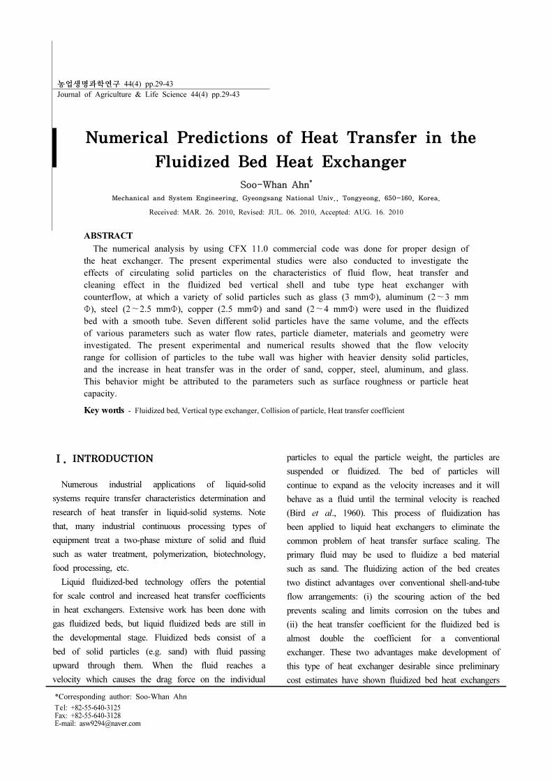
are cost competitive with conventional units as shown

in “Fig. 1.”

Fig. 1. Vertical liquid fluidized bed type and typical type shell and tube heat exchanger.

A number of studies on heat transfer in liquid

fluidized beds dealt exclusively with heat transfer, either

from a tube wall to liquid or from a heated object to

liquid in vertical cylindrical glass vessels of small scale.

The concept of a liquid-solid fluidized bed heat

exchanger was proposed by Klaren (1975) for sea water

desalination in the early 1970s. The proposed heat

exchanger consists of one or more vertical tubes in

which an upward flowing fouling liquid fluidizes inert

particles. For liquid-solid fluidized beds Richardson et

al. (1976) found that heat transfer coefficients are up to

8 times higher than for single phase flow at the same

velocity. The same author accented that particles in

suspension have scouring action because they reduce the

formation of deposits on the heat transfer surfaces.

Experimental studies by Haid et al. (1994) have shown

that the presence of solid particles in fluidized beds can

significantly enhance wall-to-bed heat transfer

coefficients, compared to flow without particles.

Moreover the fluidized bed heat exchangers were used

to prevent fouling in various process applications

(Rautenbach & Katz, 1996; Klaren, 2000).

The fluidized solid particles not only increases heat

transfer rates but have a cleaning function eliminating

contained substances caused from condensate water. For

proper design of a circulating fluidized bed heat

exchanger it is important to know the effect of design

and operating parameters on the bed to the wall heat

transfer coefficient.

In the present work, experimental and numerical

studies have been conducted to examine the

characteristics of fluid flow and heat transfer in a

vertical fluidized bed shell and tube type heat

exchanger with counterflow, at which 7 different solid

particles in water are circulated.

Ⅱ. EXPERIMENTAL SETUP

The heat transfer and fouling eliminating experiments

were conducted with seven different particles transported

and fluidized with water as shown in Figs. 1 and 2 (L

– heat transfer setup; R–visualization setup). Seven

different particles such as glass (bed, 3 mmΦ),

aluminum (cylinder, 2 mm and 3 mmΦ), copper

(cylinder, 2.5 mmΦ), steel (cylinder, 2 mm and 2.5

mmΦ) and sand (grain, 2~4 mmΦ) were used (see

Table 1). In case of stainless steel or aluminum,

particles are generally made of wire and are therefore

cylindrically shaped; glass particles are mostly spherical.

All the particles had the same volume of 14 mm3

except the sand and the volume fraction of solid

particles in the test section were maintained 1.4%. The

particles are circulated by installing the plate with same

size holes as tube diameters in the in let. When a

particle moves downward through the vertical tube, the

collision of particle to the tube wall hardly occurs.

Therefore, in order to make a high frequency of the

collision, the heat exchanger is designated that

two-sided tubes have upperward particle movements and

a core tube has a downward particle movement. The

dimensions of the heat exchanger were 705 mm in

Ahn : Numerical Predictions of Heat Transfer in the Fluidized Bed Heat Exchanger … 31

height, 80.4 mm in shell diameter. The tubes for heat

transfer and visualization have same inner diameter of

14.2 mm. Flow rate was controlled by the valves which

bypassed a relevant amount of water back to a

reservoir, and the fluid flow rate in the tube was

measured with cumulative type flow meter. Downstream

of the test section, a condensing coil was installed to

maintain the constant temperature of circulating fluid at

the entrance of test section. The test section and the

fluidized bed heat exchanger (see the right hand side in

Fig. 2. were fabricated with a transparent acrylic

material for CCD camera. The heat transfer test section

(left hand side) was made of stainless steel in the shell

and copper in the tubes. The inlet and outlet

temperatures of cold water correspond to 26~28℃ and

31~40℃, respectively. And the inlet and outlet

temperatures of hot water in the shell side become

83~75℃ and 71~51℃. The wall temperature (Tw) is

measured by three thermocouples with beads buried

inside the tube thickness starting 14 cm downstream of

the inlet. The water temperatures are measured by

thermocouples placed at inlet and outlet of the test

section. The local water temperature along the axial

distance is estimated by linear interpolation between the

measured inlet and exit temperatures. The velocity in

the sided tubes of heat transfer experiment were read

from the water head in two calibration tubes of a

single tube (center) and a visualization test section.

Table 1. Details of particles

Classification DimensionThermal

conductivity(W/m K)

Density(kg/m3)

Glass Bead 3 mmΦ 1.2 2225

Aluminum 2 mmΦ 237 2702

Aluminum 3 mmΦ 237 2702

Steel 2 mmΦ 80.2 7870

Steel 2.5 mmΦ 80.2 7870

Copper 2.5 mmΦ 401 8933

Sand 3 mmΦ 1.8 1515

The equality between heat transfer rate in the tube

side (Qc) and heat transfer rate in the shell (Qh) was

not allowed in the present fluidized bed shell and tube

type heat exchanger because the range of fluid velocity

for possible particle collision to the wall is very

restricted. Therefore, the heat transfer coefficient (hc)

for tubes in the shell and tube type heat exchanger was

obtained from the preparatory experimental section

where the hot water inlet and outlet valves are shut

down in Fig. 2. The heat transfer coefficient for tubes

(hc) was obtained from the measured temperatures and

flow rates in the preparatory sections where the hot

water inlet and outlet valves in Fig. 2. are shut down

as follows:

)](/[ fwc TTDLQh −= π (1)

)( inoutp TTcmQ −= & (2)

Where m& , cp, D, L, Tout, Tin, Tw and Tf are the

flow rate, specific heat, inner diameter of tube, length

of tube, inlet and outlet bulk temperatures, average wall

and water temperatures, respectively. The solid particle

volume fraction of 1.4% was maintained not to

intervene with the flow in the mid tube in terms of

accumulating particles on the baffle plate. Heat transfer

rates in the tubes (Qc) and in the shell (Qh) in the

counterflow were obtained from the following equations:

)(21 ccpcc TTcmQ −= & (3)

)(21 hhphh TTcmQ −= & (4)

The effect of fluidized bed on log mean temperature

difference (LMTD) was examined, at which the water

was flowed in the velocity range of 0.2 ～ 1.5 m/s.

The log mean temperature difference (LMTD) for

counterflow defined as

)/()ln[(

)()(

1221

1221

chch

chch

TTTT

TTTTLMTD

−−

−−−

=

(5)


T

Hotwater

T

T

T

T

T T

CalibrationHot water

Heat transfer

experiment

Visualization

experiment

Coolingwater

Condensing coil

Reservoir

Coolingwater

Calibration

5kW heater

Fluidized bedheat exchanger(Stainless steel)

Preparatoryexperiment(Copper)

Fluidized bedheat exchanger

(Acrylic)

tube

Transferpump

outlet

T Temperature measurementValveFlow meter

tube 77

487705

141

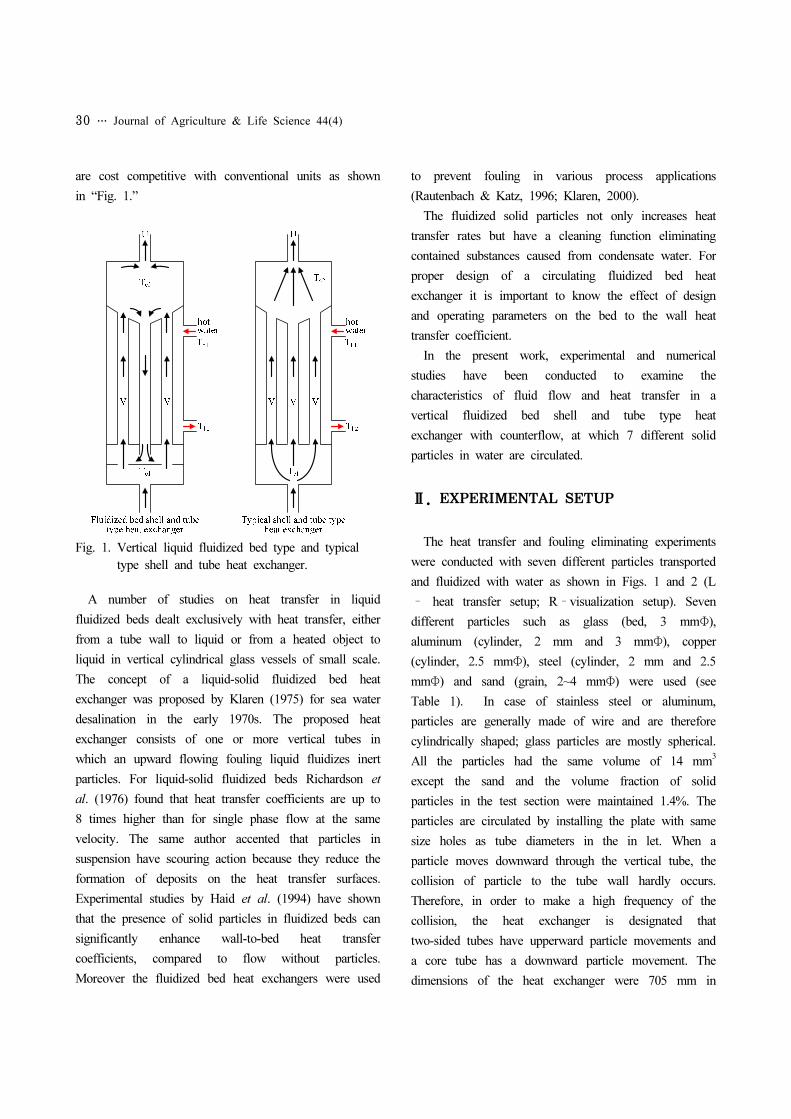
Fig. 2. Schematic diagram of experimental setup.

Here, the subscripts h and c designated the hot (shell

side) and cold (tube side) fluids and 1 and 2 means the

inlet and outlet section. D and di are diameters in the outlet

of heat exchanger and in the tube as shown in Fig. 3.

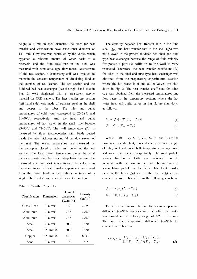
(a) distance between tube and baffle plate (b) lower side (c) upper side

Fig. 3. Configuration of test section for simulation.

Every experimental data were obtained by averaging

the ten repeated values to check out the conformity.

The experimental uncertainties were estimated using the

procedure outlined by Kline & McClintock (1953). The

maximum uncertainty in the mass flow rate•

m was

estimated to be 3.9%, resulting in the maximum

uncertainty of the convective heat transfer coefficient hc

of 6.4% at tube side water velocity of 0.6m/s.

Ⅲ. NUMERICAL METHODLOGY

3.1 PARTICLE TRANSPORT MODEL


The numerical simulations of the fluid flow and heat

transfer in the analyzed square duct geometries are

conducted with the CFX 11.0 commercial code. For the

working fluid, material properties of water are taken.

Since the description of the basic conservation equations

(mass, momentum and thermal energy) used in the code

can be found in any classical fluid dynamics textbook

or CFX manual, it is not repeated, here, but just

explained the particle transport model as well as the

shear stress transport (SST) model. The particle

transport model is capable of modeling dispersed phases

which are discretely distributed in a continuous phase.

The modeling involves the separate calculation of each

phase with source terms generated to account for the

effects of the particles on the continuous phase. The

implementation of particle transport modeling can be

thought of as a multiphase flow in which the particles

are a dispersed phase, where particulates are tracked

through the flow in a Lagrangian way, rather than

being modeled as an extra Eularian phase. The full

particulate phase is modeled by just a sample of

individual particles. The tracking is carried out by

forming a set of ordinary differential equations in time

for each particle, consisting of equations for position,

velocity, temperature, and masses of species. These

equations are then integrated using a simple integration

method to calculate the behavior of the particles as

they traverse the flow domain. All continuous phases

are treated as the Eulerian model.

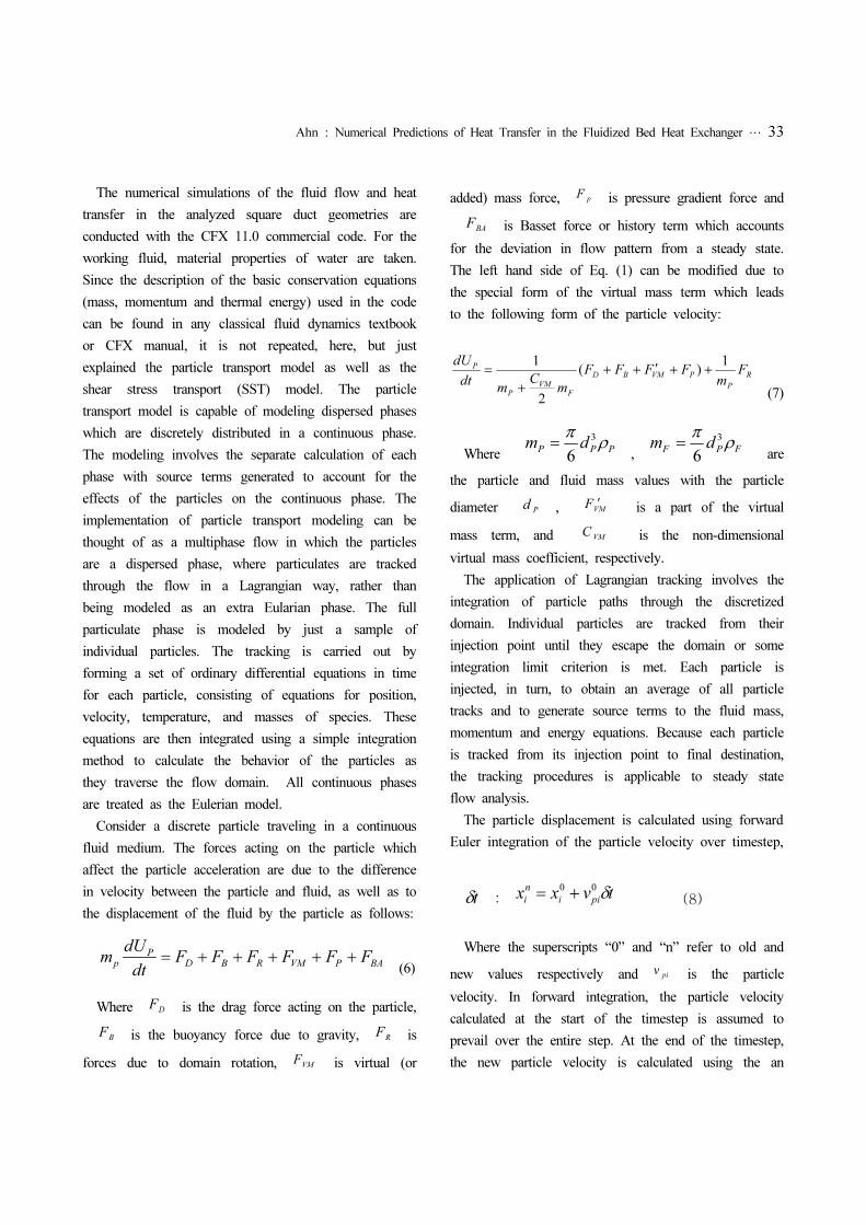
Consider a discrete particle traveling in a continuous

fluid medium. The forces acting on the particle which

affect the particle acceleration are due to the difference

in velocity between the particle and fluid, as well as to

the displacement of the fluid by the particle as follows:

BAPVMRBDP

p FFFFFFdt

dUm +++++=

(6)

Where DF is the drag force acting on the particle,

BF is the buoyancy force due to gravity, R

F is

forces due to domain rotation, VMF is virtual (or

added) mass force, pF is pressure gradient force and

BAF is Basset force or history term which accounts

for the deviation in flow pattern from a steady state.

The left hand side of Eq. (1) can be modified due to

the special form of the virtual mass term which leads

to the following form of the particle velocity:

R

P

PVMBD

F

VM

P

PF

mFFFF

mC

mdt

dU 1)(

2

1++′++

+

=

(7)

Where PPPdm ρ

π 3

6=

, FPFdm ρ

π 3

6=

are

the particle and fluid mass values with the particle

diameter Pd , VM

F ′ is a part of the virtual

mass term, and VMC is the non-dimensional

virtual mass coefficient, respectively.

The application of Lagrangian tracking involves the

integration of particle paths through the discretized

domain. Individual particles are tracked from their

injection point until they escape the domain or some

integration limit criterion is met. Each particle is

injected, in turn, to obtain an average of all particle

tracks and to generate source terms to the fluid mass,

momentum and energy equations. Because each particle

is tracked from its injection point to final destination,

the tracking procedures is applicable to steady state

flow analysis.

The particle displacement is calculated using forward

Euler integration of the particle velocity over timestep,

tδ : tvxxpii

n

iδ

00+= (8)

Where the superscripts “0” and “n” refer to old and

new values respectively and piv is the particle

velocity. In forward integration, the particle velocity

calculated at the start of the timestep is assumed to

prevail over the entire step. At the end of the timestep,

the new particle velocity is calculated using the an


alytical solution to Eq. (1) as follows:

⎟⎟⎠

⎞⎜⎜⎝

⎛⎟⎠

⎞⎜⎝

⎛−−+⎟

⎠

⎞⎜⎝

⎛−−+=

τ

δτ

τ

δ tF

tvvvv allfpfp exp1exp)( 0

(9)

The fluid properties are taken from the start of the

timestep. For the particle momentum, 0f would

correspond to the particle velocity at the start of the

timestep. In the calculation of all the forces, many fluid

variables, such as density, viscosity and velocity are

needed at the position of the particle. These variables

are always obtained accurately by calculating the

element in which the particle is traveling, calculating

the computational position within the element, and using

the underlying shape functions of the discretization

algorithm to interpolate from the vertices to the particle

position.

According to Eq. (6), the fluid affects the particle

motion through the viscous drag and a difference in

velocity between the particle and fluid. Conversely,

there is a counteracting influence of the particle on the

fluid flow due to the viscous drag. This effect is

termed coupling between the phases. If the fluid is

allowed to influence trajectories but particles do not

affect the fluid, then the interaction is termed one-way

coupling. If the particles also affect the fluid behavior,

then the interaction is termed two-way coupling.

The flow prediction of the two phases in one-way

coupled systems is relatively straightforward. The fluid

flow field may be calculated irrespective of the particle

trajectories. One-way coupling may be an acceptable

approximation in flows with low dispersed phase

loadings where particles have a negligible influence on

the fluid flow. Two-way coupling requires that the

particle source terms are included in the momentum

equations. The momentum sources could be due to

turbulent dispersion forces or drag. The particle source

terms are generated for each particle as they are

tracked through the flow. Particle sources are applied in

the control volume that the particle is in during the

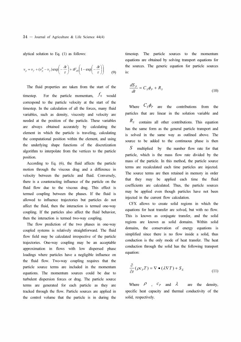
timestep. The particle sources to the momentum

equations are obtained by solving transport equations for

the sources. The generic equation for particle sources

is:

SPS

PRC

dt

dS+= φ

(10)

Where PSC φ are the contributions from the

particles that are linear in the solution variable and

SR contains all other contributions. This equation

has the same form as the general particle transport and

is solved in the same way as outlined above. The

source to be added to the continuous phase is then

S multiplied by the number flow rate for that

particle, which is the mass flow rate divided by the

mass of the particle. In this method, the particle source

terms are recalculated each time particles are injected.

The source terms are then retained in memory in order

that they may be applied each time the fluid

coefficients are calculated. Thus, the particle sources

may be applied even though particles have not been

injected in the current flow calculation.

CFX allows to create solid regions in which the

equations for heat transfer are solved, but with no flow.

This is known as conjugate transfer, and the solid

regions are known as solid domains. Within solid

domains, the conservation of energy equations is

simplified since there is no flow inside a solid, thus

conduction is the only mode of heat transfer. The heat

conduction through the solid has the following transport

equation:

EPSTTc

t+∇•∇=

∂

∂)()( λρ

(11)

Where ρ , Pc and λ are the density,

specific heat capacity and thermal conductivity of the

solid, respectively.


At a solid-fluid 1:1 interface duplicate nodes exit.

The conservative value for the solid-side node is the

variable values averaged over the half on the control

volume that lies inside the solid. The conservative value

for the fluid-side node is the variable values averaged

over the half of the control volume that lies in the

fluid. Consider the example of heat transfer from a hot

solid to a cool fluid when advection dominates within

the fluid. If a plot across the solid-fluid interface using

conservative values of temperature is created, then a

sharp change in temperature across the interface can be

seen. This is because values are interpolated from the

interface into the bulk of the solid domain using the

value for the solid-side node at the interface, while

values are interpolated from the interface into the bulk

of the fluid domain using the value for the fluid-side

node at the interface.

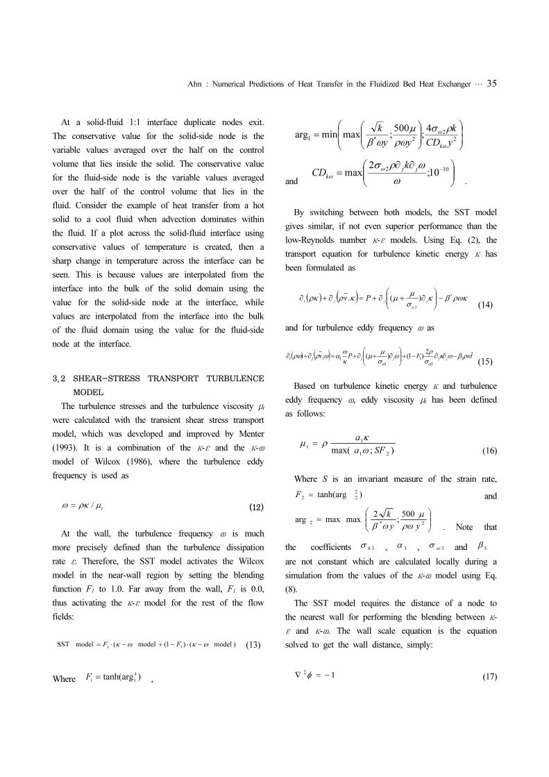
3.2 SHEAR-STRESS TRANSPORT TURBULENCE

MODEL

The turbulence stresses and the turbulence viscosity μt

were calculated with the transient shear stress transport

model, which was developed and improved by Menter

(1993). It is a combination of the κ-ε and the κ-ω

model of Wilcox (1986), where the turbulence eddy

frequency is used as

tμρκω /= (12)

At the wall, the turbulence frequency ω is much

more precisely defined than the turbulence dissipation

rate ε. Therefore, the SST model activates the Wilcox

model in the near-wall region by setting the blending

function F1 to 1.0. Far away from the wall, F1 is 0.0,

thus activating the κ-ε model for the rest of the flow

fields:

)model()1(model(modelSST11

ωκωκ −⋅−+−⋅= FF (13)

Where )tanh(arg 4

11=F ,

⎟⎟

⎠

⎞

⎜⎜

⎝

⎛

⎟⎟⎠

⎞⎜⎜⎝

⎛=

2

2

2*1

4;

500;maxminarg

yCD

k

yy

k

kω

ωρσ

ρω

μ

ωβ

and ⎟⎟⎠

⎞⎜⎜⎝

⎛ ∂∂= −102

10;2

maxω

ωρσω

ω

jj

k

kCD

.

By switching between both models, the SST model

gives similar, if not even superior performance than the

low-Reynolds number κ-ε models. Using Eq. (2), the

transport equation for turbulence kinetic energy κ has

been formulated as

( ) ( ) ρωκβκσ

μμκρρκ

κ

*

3

)( −⎟⎟⎠

⎞⎜⎜⎝

⎛∂+∂+=∂+∂

jjjjtPv

(14)

and for turbulence eddy frequency ω as

( ) ( ) 2

3

2

1

3

3

2)1()( ρωβωκσ

ρω

σ

μμ

κ

ωαωρρω

ωω

−∂∂−+⎟⎟⎠

⎞⎜⎜⎝

⎛∂+∂+=∂+∂ jjjjjjt FPv

(15)

Based on turbulence kinetic energy κ and turbulence

eddy frequency ω, eddy viscosity μt has been defined

as follows:

);max(21

1

SFa

a

t

ω

κρμ =

(16)

Where S is an invariant measure of the strain rate,

)tanh(arg 2

22=F and

⎟⎟⎠

⎞⎜⎜⎝

⎛=

2*2

500;

2maxmaxarg

yy

k

ρω

μ

ωβ . Note that

the coefficients 3kσ , 3

α , 3ωσ and 3

β

are not constant which are calculated locally during a

simulation from the values of the κ-ω model using Eq.

(8).

The SST model requires the distance of a node to

the nearest wall for performing the blending between κ-

ε and κ-ω. The wall scale equation is the equation

solved to get the wall distance, simply:

12

−=∇ φ (17)


Where φ is the value of the wall scale. The

turbulence model using in a particle tracking simulation

only applies to the continuous phases. Turbulence can

affect the particles through the particle dispersion force,

but the particles can have no effect on the turbulence

of the continuous phase, other than indirectly by

affecting the velocity field.

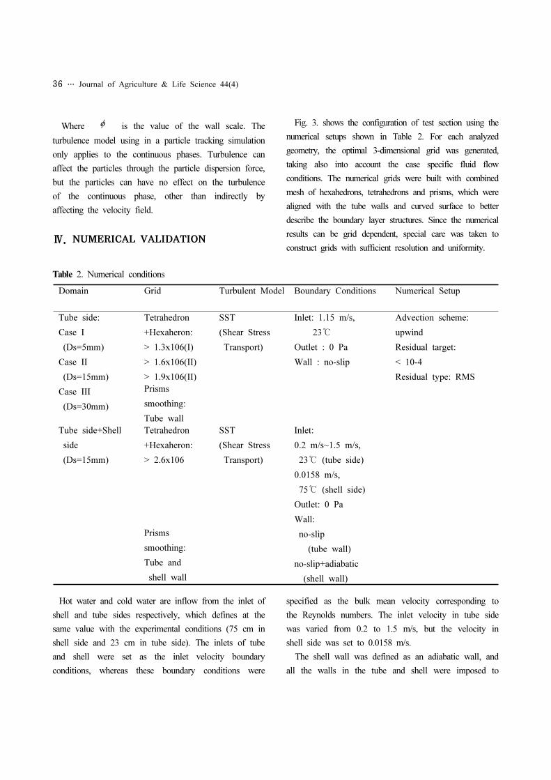
Ⅳ. NUMERICAL VALIDATION

Fig. 3. shows the configuration of test section using the

numerical setups shown in Table 2. For each analyzed

geometry, the optimal 3-dimensional grid was generated,

taking also into account the case specific fluid flow

conditions. The numerical grids were built with combined

mesh of hexahedrons, tetrahedrons and prisms, which were

aligned with the tube walls and curved surface to better

describe the boundary layer structures. Since the numerical

results can be grid dependent, special care was taken to

construct grids with sufficient resolution and uniformity.

Table 2. Numerical conditions

Domain Grid Turbulent Model Boundary Conditions Numerical Setup

Tube side:

Case I

(Ds=5mm)

Case II

(Ds=15mm)

Case III

(Ds=30mm)

Tetrahedron

+Hexaheron:

> 1.3x106(I)

> 1.6x106(II)

> 1.9x106(II)

SST

(Shear Stress

Transport)

Inlet: 1.15 m/s,

23℃

Outlet : 0 Pa

Wall : no-slip

Advection scheme:

upwind

Residual target:

< 10-4

Residual type: RMSPrisms

smoothing:

Tube wallTube side+Shell

side

(Ds=15mm)

Tetrahedron

+Hexaheron:

> 2.6x106

SST

(Shear Stress

Transport)

Inlet:

0.2 m/s~1.5 m/s,

23℃ (tube side)

0.0158 m/s,

75℃ (shell side)

Outlet: 0 Pa

Wall:

no-slip

(tube wall)

no-slip+adiabatic

(shell wall)

Prisms

smoothing:

Tube and

shell wall

Hot water and cold water are inflow from the inlet of

shell and tube sides respectively, which defines at the

same value with the experimental conditions (75 cm in

shell side and 23 cm in tube side). The inlets of tube

and shell were set as the inlet velocity boundary

conditions, whereas these boundary conditions were

specified as the bulk mean velocity corresponding to

the Reynolds numbers. The inlet velocity in tube side

was varied from 0.2 to 1.5 m/s, but the velocity in

shell side was set to 0.0158 m/s.

The shell wall was defined as an adiabatic wall, and

all the walls in the tube and shell were imposed to


no-slip boundary conditions. In the inlet boundary

condition of tube side, the setting of turbulent intensity

plays an important role in influencing the heat transfer

behaviors. It is found that the turbulent intensity

( Uu /2' ) of 5% was suitable for this

simulation (Kim et al., 1994). A particle is assumed to

be spherical type, where the diameter of the particle is

calculated from the mass of the particle divided by its

density. A constant time step of 0.0001 s was used

for all cases.

In order to capture the thermal layers and the

transitional boundary layers correctly, the grid must

have a y+ ( μρ

τ/yuΔ= )of approximately one.

One of the well known deficiencies of the k-ε model is

its inability to handle low turbulent Reynolds number

computations. Complex damping functions can be added

to the k-ε model, as well as the requirement of highly

refined near-wall grid resolution (y+ < 0.2) in an

attempt to model low turbulent Reynolds number flows

or high wall heat transfer. This approach often leads to

numerical instability. Some of these difficulties may be

avoided by using the k-ω model, making it more

appropriate than the k-ε model for flows requiring high

near-wall resolution. However, a strict low-Reynolds

number implementation of the model would also require

a near wall grid resolution of at least y+ < 2.0. This

condition cannot be guaranteed in most applications at

all walls. For this reason, a new near wall treatment

for high accuracy boundary layer simulations was

developed by CFX for the k-ω based

Shear-Stress-Transport(SST) turbulence model that allows

for a smooth shift from a low-Reynolds number form

to a wall function formulations.

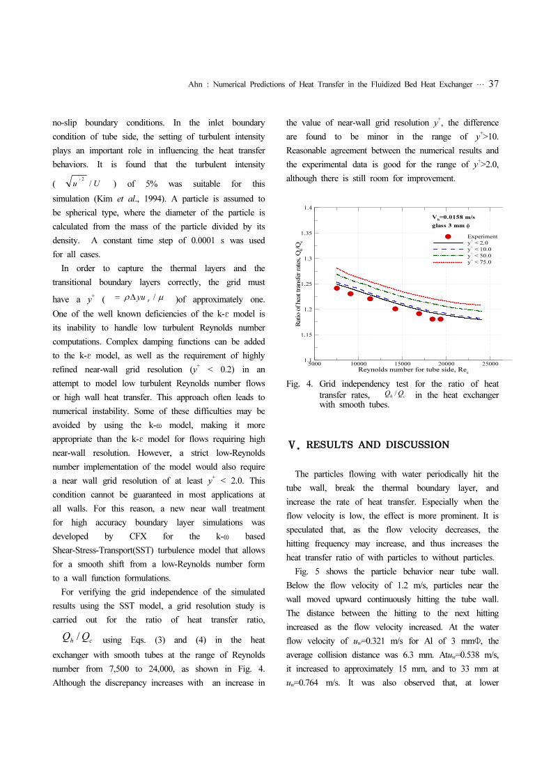
For verifying the grid independence of the simulated

results using the SST model, a grid resolution study is

carried out for the ratio of heat transfer ratio,

chQQ / using Eqs. (3) and (4) in the heat

exchanger with smooth tubes at the range of Reynolds

number from 7,500 to 24,000, as shown in Fig. 4.

Although the discrepancy increases with an increase in

the value of near-wall grid resolution y+, the difference

are found to be minor in the range of y+>10.

Reasonable agreement between the numerical results and

the experimental data is good for the range of y+>2.0,

although there is still room for improvement.

Reynolds number for tube side, Rec

Ratioofheattransferrates,Qh/Q

c

5000 10000 15000 20000 250001.1

1.15

1.2

1.25

1.3

1.35

1.4

Experiment

y+

< 2.0

y+

< 10.0

y+

< 50.0

y+

< 75.0

Vh=0.0158 m/s

glass 3 mm φ

Fig. 4. Grid independency test for the ratio of heat transfer rates, ch

QQ / in the heat exchanger with smooth tubes.

Ⅴ. RESULTS AND DISCUSSION

The particles flowing with water periodically hit the

tube wall, break the thermal boundary layer, and

increase the rate of heat transfer. Especially when the

flow velocity is low, the effect is more prominent. It is

speculated that, as the flow velocity decreases, the

hitting frequency may increase, and thus increases the

heat transfer ratio of with particles to without particles.

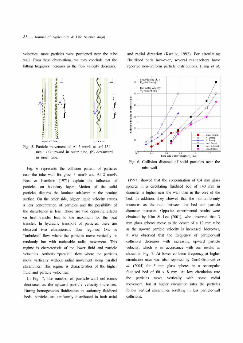
Fig. 5 shows the particle behavior near tube wall.

Below the flow velocity of 1.2 m/s, particles near the

wall moved upward continuously hitting the tube wall.

The distance between the hitting to the next hitting

increased as the flow velocity increased. At the water

flow velocity of uw=0.321 m/s for Al of 3 mmΦ, the

average collision distance was 6.3 mm. Atuw=0.538 m/s,

it increased to approximately 15 mm, and to 33 mm at

uw=0.764 m/s. It was also observed that, at lower


velocities, more particles were positioned near the tube

wall. From these observations, we may conclude that the

hitting frequency increases as the flow velocity decreases.

(a) 0.2 ~ 0.7 sec

Fig. 5. Particle movement of Al 3 mmΦ at u=1.154 m/s : (a) upward in outer tube, (b) downward in inner tube.

Fig. 6 represents the collision pattern of particles

near the tube wall for glass 3 mmΦ and Al 2 mmΦ.

Brea & Hamilton (1971) explain the influence of

particles on boundary layer. Motion of the solid

particles disturbs the laminar sub-layer at the heating

surface. On the other side, higher liquid velocity causes

a less concentration of particles and the possibility of

the disturbance is less. These are two opposing effects

on heat transfer lead to the maximum for the heat

transfer. In hydraulic transport of particles, there are

observed two characteristic flow regimes: One is

“turbulent” flow where the particles move vertically or

randomly but with noticeable radial movement. This

regime is characteristic of the lower fluid and particle

velocities. Antheris “parallel” flow where the particles

move vertically without radial movement along parallel

streamlines. This regime is characteristics of the higher

fluid and particle velocities.

In Fig. 7, the number of particle-wall collisions

decreases as the upward particle velocity increases.

During homogeneous fluidization in stationary fluidized

beds, particles are uniformly distributed in both axial

and radial direction (Kwauk, 1992). For circulating

fluidized beds however, several researchers have

reported non-uniform particle distributions. Liang et al.

Tube side water velocity, Vc(m/s)

Collisiondistanceofparticles(mm)

0.2 0.4 0.6 0.8 1 1.20

10

20

30

40

50

60

glass 3mmφAl 2mmφAl 3mmφsteel 2mmφsteel 2.5mmφCu 2.5mmφ

Smooth tube (S0)

Dvi=14.2 mmφ

Hot water velocityV

h=0.0158 m/s

Fig. 6. Collision distance of solid particles near the

tube wall.

(1997) showed that the concentration of 0.4 mm glass

spheres in a circulating fluidized bed of 140 mm in

diameter is higher near the wall than in the core of the

bed. In addition, they showed that the non-uniformity

increases as the ratio between the bed and particle

diameter increases. Opposite experimental results were

obtained by Kim & Lee (2001), who observed that 3

mm glass spheres move to the center of a 12 mm tube

as the upward particle velocity is increased. Moreover,

it was observed that the frequency of particle-wall

collisions decreases with increasing upward particle

velocity, which is in accordance with our results as

shown in Fig. 7. At lower collision frequency at higher

circulation rates was also reported by Garić-Grulović et

al. (2004) for 5 mm glass spheres in a rectangular

fluidized bed of 60 x 8 mm. At low circulation rate

the particles move vertically with some radial

movement, but at higher circulation rates the particles

follow vertical streamlines resulting in less particle-wall

collisions.


Water velocity, m/s

No.ofcollisionper

1centimeter

0 0.2 0.4 0.6 0.8 1 1.2 1.40

1

2

3

4

glass bead 3 mmφ

Al cylinder 3 mmφ

Cu cylinder 2.5 mmφ

Lee et al. (glass bead 3 mmφ)

Fig. 7. Collision pattern of the particles near the tube wall for various particles.

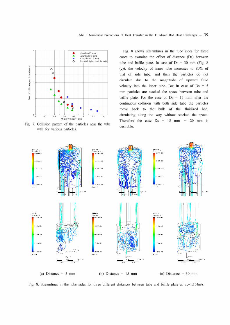
Fig. 8 shows streamlines in the tube sides for three

cases to examine the effect of distance (Ds) between

tube and baffle plate. In case of Ds = 30 mm (Fig. 8

(c)), the velocity of inner tube increases to 80% of

that of side tube, and then the particles do not

circulate due to the magnitude of upward fluid

velocity into the inner tube. But in case of Ds = 5

mm particles are stacked the space between tube and

baffle plate. For the case of Ds = 15 mm, after the

continuous collision with both side tube the particles

move back to the bulk of the fluidized bed,

circulating along the way without stacked the space.

Therefore the case Ds = 15 mm ～ 20 mm is

desirable.

(a) Distance = 5 mm (b) Distance = 15 mm (c) Distance = 30 mm

Fig. 8. Streamlines in the tube sides for three different distances between tube and baffle plate at uw=1.154m/s.


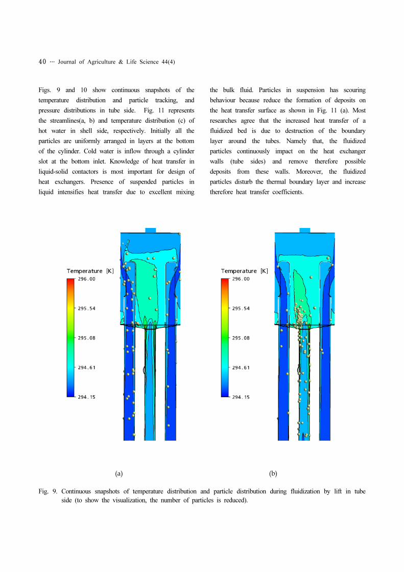
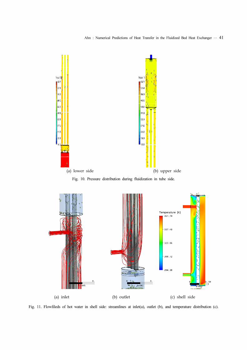
Figs. 9 and 10 show continuous snapshots of the

temperature distribution and particle tracking, and

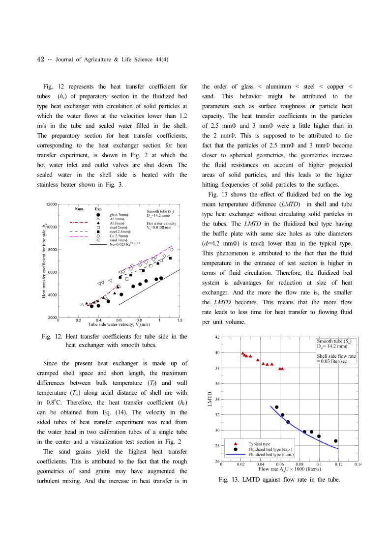
pressure distributions in tube side. Fig. 11 represents

the streamlines(a, b) and temperature distribution (c) of

hot water in shell side, respectively. Initially all the

particles are uniformly arranged in layers at the bottom

of the cylinder. Cold water is inflow through a cylinder

slot at the bottom inlet. Knowledge of heat transfer in

liquid-solid contactors is most important for design of

heat exchangers. Presence of suspended particles in

liquid intensifies heat transfer due to excellent mixing

the bulk fluid. Particles in suspension has scouring

behaviour because reduce the formation of deposits on

the heat transfer surface as shown in Fig. 11 (a). Most

researches agree that the increased heat transfer of a

fluidized bed is due to destruction of the boundary

layer around the tubes. Namely that, the fluidized

particles continuously impact on the heat exchanger

walls (tube sides) and remove therefore possible

deposits from these walls. Moreover, the fluidized

particles disturb the thermal boundary layer and increase

therefore heat transfer coefficients.

(a) (b)

Fig. 9. Continuous snapshots of temperature distribution and particle distribution during fluidization by lift in tube side (to show the visualization, the number of particles is reduced).


(a) lower side (b) upper side

Fig. 10. Pressure distribution during fluidization in tube side.

(a) inlet (b) outlet (c) shell side

Fig. 11. Flowfileds of hot water in shell side: streamlines at inlet(a), outlet (b), and temperature distribution (c).


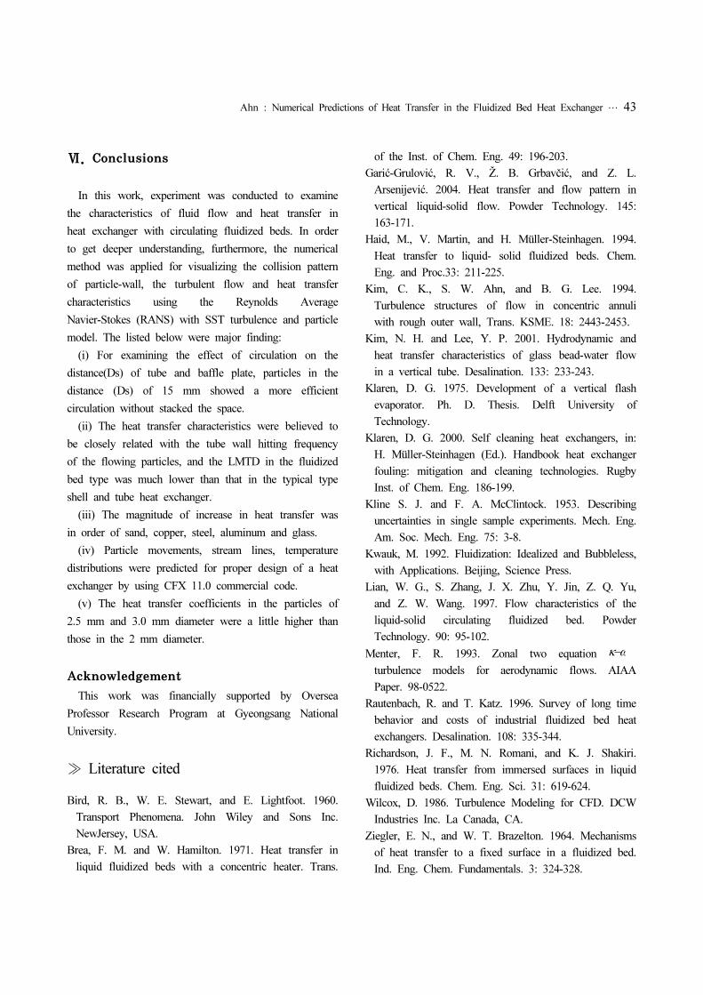
Fig. 12 represents the heat transfer coefficient for

tubes (hc) of preparatory section in the fluidized bed

type heat exchanger with circulation of solid particles at

which the water flows at the velocities lower than 1.2

m/s in the tube and sealed water filled in the shell.

The preparatory section for heat transfer coefficients,

corresponding to the heat exchanger section for heat

transfer experiment, is shown in Fig. 2 at which the

hot water inlet and outlet valves are shut down. The

sealed water in the shell side is heated with the

stainless heater shown in Fig. 3.

Tube side water velocity, Vc(m/s)

Heattransfercoefficientfortubeside,hc

0 0.2 0.4 0.6 0.8 1 1.22000

4000

6000

8000

10000

12000

glass 3mmφAl 2mmφAl 3mmφsteel 2mmφsteel 2.5mmφCu 2.5mmφsand 3mmφNu=0.023 Re

0.8Pr

0.4

Smooth tube (So)

Dvi=14.2 mmφ

Hot water velocityV

h=0.0158 m/s

Num. Exp.

Fig. 12. Heat transfer coefficients for tube side in the heat exchanger with smooth tubes.

Since the present heat exchanger is made up of

cramped shell space and short length, the maximum

differences between bulk temperature (Tf) and wall

temperature (Tw) along axial distance of shell are with

in 0.8oC. Therefore, the heat transfer coefficient (hc)

can be obtained from Eq. (14). The velocity in the

sided tubes of heat transfer experiment was read from

the water head in two calibration tubes of a single tube

in the center and a visualization test section in Fig. 2

The sand grains yield the highest heat transfer

coefficients. This is attributed to the fact that the rough

geometries of sand grains may have augmented the

turbulent mixing. And the increase in heat transfer is in

the order of glass < aluminum < steel < copper <

sand. This behavior might be attributed to the

parameters such as surface roughness or particle heat

capacity. The heat transfer coefficients in the particles

of 2.5 mmΦ and 3 mmΦ were a little higher than in

the 2 mmΦ. This is supposed to be attributed to the

fact that the particles of 2.5 mmΦ and 3 mmΦ become

closer to spherical geometries, the geometries increase

the fluid resistances on account of higher projected

areas of solid particles, and this leads to the higher

hitting frequencies of solid particles to the surfaces.

Fig. 13 shows the effect of fluidized bed on the log

mean temperature difference (LMTD) in shell and tube

type heat exchanger without circulating solid particles in

the tubes. The LMTD in the fluidized bed type having

the baffle plate with same size holes as tube diameters

(di=4.2 mmΦ) is much lower than in the typical type.

This phenomenon is attributed to the fact that the fluid

temperature in the entrance of test section is higher in

terms of fluid circulation. Therefore, the fluidized bed

system is advantages for reduction at size of heat

exchanger. And the more the flow rate is, the smaller

the LMTD becomes. This means that the more flow

rate leads to less time for heat transfer to flowing fluid

per unit volume.

Flow rate AuU × 1000 (liter/s)

LMTD

0 0.02 0.04 0.06 0.08 0.1 0.12 0.1426

28

30

32

34

36

38

40

42

Typical type

Fluidized bed type (exp.)

Fluidized bed type (num.)

Smooth tube (So)

Dvi= 14.2 mmφ

Shell side flow rate= 0.03 liter/sec

Fig. 13. LMTD against flow rate in the tube.


Ⅵ. Conclusions

In this work, experiment was conducted to examine

the characteristics of fluid flow and heat transfer in

heat exchanger with circulating fluidized beds. In order

to get deeper understanding, furthermore, the numerical

method was applied for visualizing the collision pattern

of particle-wall, the turbulent flow and heat transfer

characteristics using the Reynolds Average

Navier-Stokes (RANS) with SST turbulence and particle

model. The listed below were major finding:

(i) For examining the effect of circulation on the

distance(Ds) of tube and baffle plate, particles in the

distance (Ds) of 15 mm showed a more efficient

circulation without stacked the space.

(ii) The heat transfer characteristics were believed to

be closely related with the tube wall hitting frequency

of the flowing particles, and the LMTD in the fluidized

bed type was much lower than that in the typical type

shell and tube heat exchanger.

(iii) The magnitude of increase in heat transfer was

in order of sand, copper, steel, aluminum and glass.

(iv) Particle movements, stream lines, temperature

distributions were predicted for proper design of a heat

exchanger by using CFX 11.0 commercial code.

(v) The heat transfer coefficients in the particles of

2.5 mm and 3.0 mm diameter were a little higher than

those in the 2 mm diameter.

Acknowledgement

This work was financially supported by Oversea

Professor Research Program at Gyeongsang National

University.

≫ Literature cited

Bird, R. B., W. E. Stewart, and E. Lightfoot. 1960.

Transport Phenomena. John Wiley and Sons Inc.

NewJersey, USA.

Brea, F. M. and W. Hamilton. 1971. Heat transfer in

liquid fluidized beds with a concentric heater. Trans.

of the Inst. of Chem. Eng. 49: 196-203.

Garić-Grulović, R. V., Ž. B. Grbavčić, and Z. L.

Arsenijević. 2004. Heat transfer and flow pattern in

vertical liquid-solid flow. Powder Technology. 145:

163-171.

Haid, M., V. Martin, and H. Müller-Steinhagen. 1994.

Heat transfer to liquid- solid fluidized beds. Chem.

Eng. and Proc.33: 211-225.

Kim, C. K., S. W. Ahn, and B. G. Lee. 1994.

Turbulence structures of flow in concentric annuli

with rough outer wall, Trans. KSME. 18: 2443-2453.

Kim, N. H. and Lee, Y. P. 2001. Hydrodynamic and

heat transfer characteristics of glass bead-water flow

in a vertical tube. Desalination. 133: 233-243.

Klaren, D. G. 1975. Development of a vertical flash

evaporator. Ph. D. Thesis. Delft University of

Technology.

Klaren, D. G. 2000. Self cleaning heat exchangers, in:

H. Müller-Steinhagen (Ed.). Handbook heat exchanger

fouling: mitigation and cleaning technologies. Rugby

Inst. of Chem. Eng. 186-199.

Kline S. J. and F. A. McClintock. 1953. Describing

uncertainties in single sample experiments. Mech. Eng.

Am. Soc. Mech. Eng. 75: 3-8.

Kwauk, M. 1992. Fluidization: Idealized and Bubbleless,

with Applications. Beijing, Science Press.

Lian, W. G., S. Zhang, J. X. Zhu, Y. Jin, Z. Q. Yu,

and Z. W. Wang. 1997. Flow characteristics of the

liquid-solid circulating fluidized bed. Powder

Technology. 90: 95-102.

Menter, F. R. 1993. Zonal two equation ωκ−

turbulence models for aerodynamic flows. AIAA

Paper. 98-0522.

Rautenbach, R. and T. Katz. 1996. Survey of long time

behavior and costs of industrial fluidized bed heat

exchangers. Desalination. 108: 335-344.

Richardson, J. F., M. N. Romani, and K. J. Shakiri.

1976. Heat transfer from immersed surfaces in liquid

fluidized beds. Chem. Eng. Sci. 31: 619-624.

Wilcox, D. 1986. Turbulence Modeling for CFD. DCW

Industries Inc. La Canada, CA.

Ziegler, E. N., and W. T. Brazelton. 1964. Mechanisms

of heat transfer to a fixed surface in a fluidized bed.

Ind. Eng. Chem. Fundamentals. 3: 324-328.

Documents

Numerical Predictions of Heat Transfer in the Fluidized Bed Heat Exchangerials.gnu.ac.kr/gnuboard4/data/paper/%C1%A644%B1%… · · 2011-01-21effects of circulating solid particles