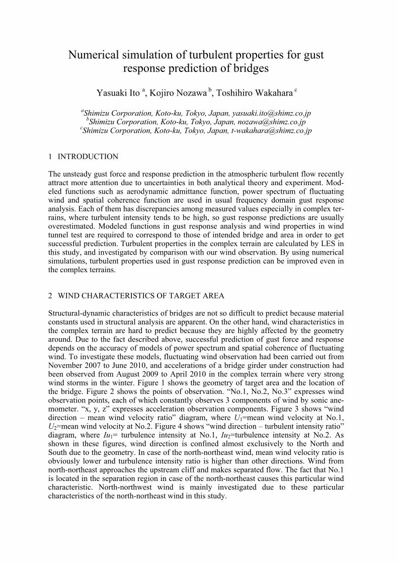
Numerical simulation of turbulent properties for gust response prediction of bridges

Yasuaki Ito a, Kojiro Nozawa b, Toshihiro Wakahara c

aShimizu Corporation, Koto-ku, Tokyo, Japan, yasuaki.ito@shimz.co.jp bShimizu Corporation, Koto-ku, Tokyo, Japan, nozawa@shimz.co.jp

cShimizu Corporation, Koto-ku, Tokyo, Japan, t-wakahara@shimz.co.jp

1 INTRODUCTION

The unsteady gust force and response prediction in the atmospheric turbulent flow recently attract more attention due to uncertainties in both analytical theory and experiment. Mod-eled functions such as aerodynamic admittance function, power spectrum of fluctuating wind and spatial coherence function are used in usual frequency domain gust response analysis. Each of them has discrepancies among measured values especially in complex ter-rains, where turbulent intensity tends to be high, so gust response predictions are usually overestimated. Modeled functions in gust response analysis and wind properties in wind tunnel test are required to correspond to those of intended bridge and area in order to get successful prediction. Turbulent properties in the complex terrain are calculated by LES in this study, and investigated by comparison with our wind observation. By using numerical simulations, turbulent properties used in gust response prediction can be improved even in the complex terrains.

2 WIND CHARACTERISTICS OF TARGET AREA

Structural-dynamic characteristics of bridges are not so difficult to predict because material constants used in structural analysis are apparent. On the other hand, wind characteristics in the complex terrain are hard to predict because they are highly affected by the geometry around. Due to the fact described above, successful prediction of gust force and response depends on the accuracy of models of power spectrum and spatial coherence of fluctuating wind. To investigate these models, fluctuating wind observation had been carried out from November 2007 to June 2010, and accelerations of a bridge girder under construction had been observed from August 2009 to April 2010 in the complex terrain where very strong wind storms in the winter. Figure 1 shows the geometry of target area and the location of the bridge. Figure 2 shows the points of observation. “No.1, No.2, No.3” expresses wind observation points, each of which constantly observes 3 components of wind by sonic ane-mometer. “x, y, z” expresses acceleration observation components. Figure 3 shows “wind direction – mean wind velocity ratio” diagram, where U1=mean wind velocity at No.1, U2=mean wind velocity at No.2. Figure 4 shows “wind direction – turbulent intensity ratio” diagram, where Iu1= turbulence intensity at No.1, Iu2=turbulence intensity at No.2. As shown in these figures, wind direction is confined almost exclusively to the North and South due to the geometry. In case of the north-northeast wind, mean wind velocity ratio is obviously lower and turbulence intensity ratio is higher than other directions. Wind from north-northeast approaches the upstream cliff and makes separated flow. The fact that No.1 is located in the separation region in case of the north-northeast causes this particular wind characteristic. North-northwest wind is mainly investigated due to these particular characteristics of the north-northeast wind in this study.

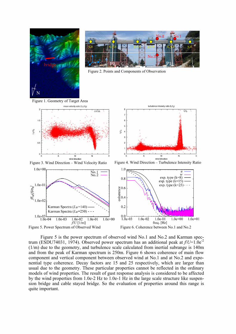
Figure 5. Power Spectrum of Observed Wind Figure 6. Coherence between No.1 and No.2

Figure 5 is the power spectrum of observed wind No.1 and No.2 and Karman spec-trum (ESDU74031, 1974). Observed power spectrum has an additional peak at f/U=1.0e-2 (1/m) due to the geometry, and turbulence scale calculated from inertial subrange is 140m and from the peak of Karman spectrum is 250m. Figure 6 shows coherence of main flow component and vertical component between observed wind at No.1 and at No.2 and expo-nential type coherence. Decay factors are 15 and 25 respectively, which are larger than usual due to the geometry. These particular properties cannot be reflected in the ordinary models of wind properties. The result of gust response analysis is considered to be affected by the wind properties from 1.0e-2 Hz to 1.0e-1 Hz in the large scale structure like suspen-sion bridge and cable stayed bridge. So the evaluation of properties around this range is quite important.

P2 P1

x,y,z

y z x

y,z y,y,z y,y,z x,y,z y,z

No.1 No.2

No.3

Figure 1. Geometry of Target Area

Figure 2. Points and Components of Observation

Figure 3. Wind Direction – Wind Velocity Ratio Figure 4. Wind Direction – Turbulence Intensity Ratio

bridge

N

3 FREQUENCY DOMAIN GUST RESPONSE ANALYSIS

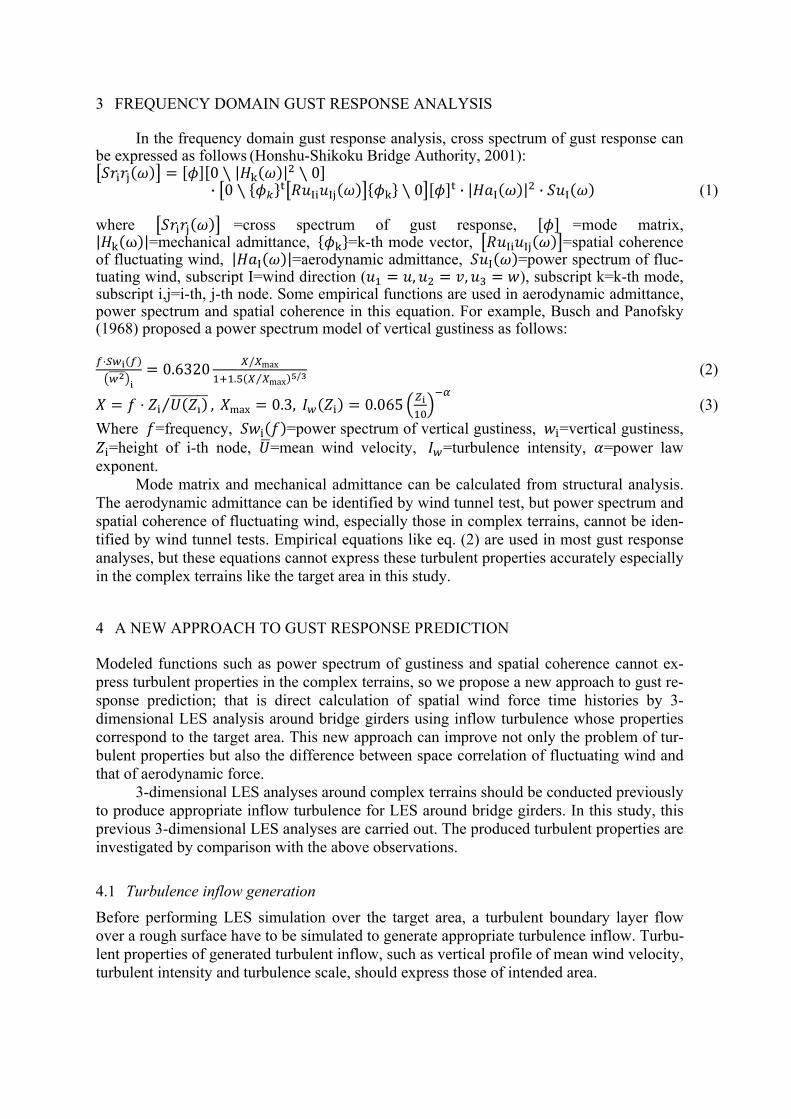
In the frequency domain gust response analysis, cross spectrum of gust response can be expressed as follows (Honshu-Shikoku Bridge Authority, 2001):

0 | | 0 · 0 I I 0 · | I | · I (1)

where =cross spectrum of gust response, =mode matrix, | ω |=mechanical admittance, =k-th mode vector, I I =spatial coherence of fluctuating wind, | I |=aerodynamic admittance, I =power spectrum of fluc-tuating wind, subscript I=wind direction ( , , ), subscript k=k-th mode, subscript i,j=i-th, j-th node. Some empirical functions are used in aerodynamic admittance, power spectrum and spatial coherence in this equation. For example, Busch and Panofsky (1968) proposed a power spectrum model of vertical gustiness as follows:

0.6320 / max

. max⁄ /   (2)

⁄ ,   max 0.3,   0.065 (3) Where =frequency, =power spectrum of vertical gustiness, =vertical gustiness,

=height of i-th node, =mean wind velocity,   =turbulence intensity, =power law exponent. Mode matrix and mechanical admittance can be calculated from structural analysis. The aerodynamic admittance can be identified by wind tunnel test, but power spectrum and spatial coherence of fluctuating wind, especially those in complex terrains, cannot be iden-tified by wind tunnel tests. Empirical equations like eq. (2) are used in most gust response analyses, but these equations cannot express these turbulent properties accurately especially in the complex terrains like the target area in this study.

4 A NEW APPROACH TO GUST RESPONSE PREDICTION

Modeled functions such as power spectrum of gustiness and spatial coherence cannot ex-press turbulent properties in the complex terrains, so we propose a new approach to gust re-sponse prediction; that is direct calculation of spatial wind force time histories by 3-dimensional LES analysis around bridge girders using inflow turbulence whose properties correspond to the target area. This new approach can improve not only the problem of tur-bulent properties but also the difference between space correlation of fluctuating wind and that of aerodynamic force. 3-dimensional LES analyses around complex terrains should be conducted previously to produce appropriate inflow turbulence for LES around bridge girders. In this study, this previous 3-dimensional LES analyses are carried out. The produced turbulent properties are investigated by comparison with the above observations.

4.1 Turbulence inflow generation Before performing LES simulation over the target area, a turbulent boundary layer flow over a rough surface have to be simulated to generate appropriate turbulence inflow. Turbu-lent properties of generated turbulent inflow, such as vertical profile of mean wind velocity, turbulent intensity and turbulence scale, should express those of intended area.

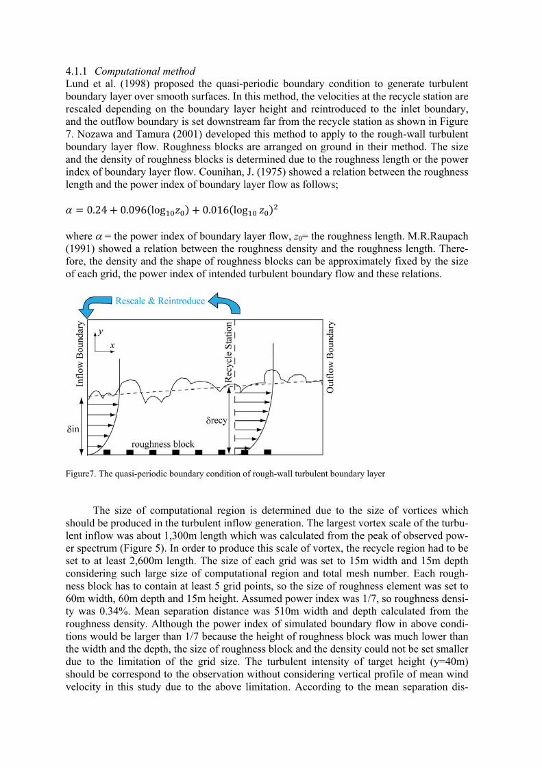
4.1.1 Computational method Lund et al. (1998) proposed the quasi-periodic boundary condition to generate turbulent boundary layer over smooth surfaces. In this method, the velocities at the recycle station are rescaled depending on the boundary layer height and reintroduced to the inlet boundary, and the outflow boundary is set downstream far from the recycle station as shown in Figure 7. Nozawa and Tamura (2001) developed this method to apply to the rough-wall turbulent boundary layer flow. Roughness blocks are arranged on ground in their method. The size and the density of roughness blocks is determined due to the roughness length or the power index of boundary layer flow. Counihan, J. (1975) showed a relation between the roughness length and the power index of boundary layer flow as follows;

0.24 0.096 log 0.016 log where α = the power index of boundary layer flow, z0= the roughness length. M.R.Raupach (1991) showed a relation between the roughness density and the roughness length. There-fore, the density and the shape of roughness blocks can be approximately fixed by the size of each grid, the power index of intended turbulent boundary flow and these relations.

Figure7. The quasi-periodic boundary condition of rough-wall turbulent boundary layer

The size of computational region is determined due to the size of vortices which should be produced in the turbulent inflow generation. The largest vortex scale of the turbu-lent inflow was about 1,300m length which was calculated from the peak of observed pow-er spectrum (Figure 5). In order to produce this scale of vortex, the recycle region had to be set to at least 2,600m length. The size of each grid was set to 15m width and 15m depth considering such large size of computational region and total mesh number. Each rough-ness block has to contain at least 5 grid points, so the size of roughness element was set to 60m width, 60m depth and 15m height. Assumed power index was 1/7, so roughness densi-ty was 0.34%. Mean separation distance was 510m width and depth calculated from the roughness density. Although the power index of simulated boundary flow in above condi-tions would be larger than 1/7 because the height of roughness block was much lower than the width and the depth, the size of roughness block and the density could not be set smaller due to the limitation of the grid size. The turbulent intensity of target height (y=40m) should be correspond to the observation without considering vertical profile of mean wind velocity in this study due to the above limitation. According to the mean separation dis-

tance, the recycle region was finally set to 3,060m and the computational region to 4,590m length, 2,550m width, and 2,000m height, and mesh size was 306x170x120.

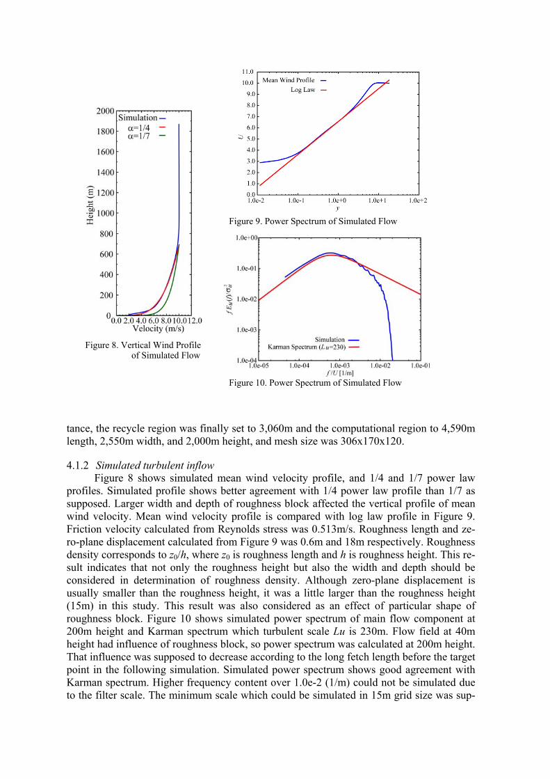
4.1.2 Simulated turbulent inflow Figure 8 shows simulated mean wind velocity profile, and 1/4 and 1/7 power law

profiles. Simulated profile shows better agreement with 1/4 power law profile than 1/7 as supposed. Larger width and depth of roughness block affected the vertical profile of mean wind velocity. Mean wind velocity profile is compared with log law profile in Figure 9. Friction velocity calculated from Reynolds stress was 0.513m/s. Roughness length and ze-ro-plane displacement calculated from Figure 9 was 0.6m and 18m respectively. Roughness density corresponds to z0/h, where z0 is roughness length and h is roughness height. This re-sult indicates that not only the roughness height but also the width and depth should be considered in determination of roughness density. Although zero-plane displacement is usually smaller than the roughness height, it was a little larger than the roughness height (15m) in this study. This result was also considered as an effect of particular shape of roughness block. Figure 10 shows simulated power spectrum of main flow component at 200m height and Karman spectrum which turbulent scale Lu is 230m. Flow field at 40m height had influence of roughness block, so power spectrum was calculated at 200m height. That influence was supposed to decrease according to the long fetch length before the target point in the following simulation. Simulated power spectrum shows good agreement with Karman spectrum. Higher frequency content over 1.0e-2 (1/m) could not be simulated due to the filter scale. The minimum scale which could be simulated in 15m grid size was sup-

Figure 8. Vertical Wind Profile of Simulated Flow

Figure 9. Power Spectrum of Simulated Flow

Figure 10. Power Spectrum of Simulated Flow

posed to 1.0e-2 (1/m), so this result is quite reasonable comparing with the supposition. Higher frequency content over 1.0e-2 (1/m) can be produced in following simulation with much smaller grid size over the target geometry.

4.2 Numerical simulation over the complex terrain

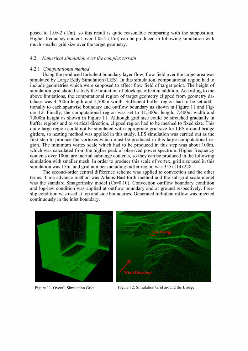
4.2.1 Computational method Using the produced turbulent boundary layer flow, flow field over the target area was simulated by Large Eddy Simulation (LES). In this simulation, computational region had to include geometries which were supposed to affect flow field of target point. The height of simulation grid should satisfy the limitation of blockage effect in addition. According to the above limitations, the computational region of target geometry clipped from geometry da-tabase was 4,700m length and 2,500m width. Sufficient buffer region had to be set addi-tionally to each spanwise boundary and outflow boundary as shown in Figure 11 and Fig-ure 12. Finally, the computational region was set to 11,300m length, 7,400m width and 7,000m height as shown in Figure 11. Although grid size could be stretched gradually in buffer regions and to vertical direction, clipped region had to be meshed to fixed size. This quite large region could not be simulated with appropriate grid size for LES around bridge girders, so nesting method was applied in this study. LES simulation was carried out as the first step to produce the vortexes which must be produced in this large computational re-gion. The minimum vortex scale which had to be produced in this step was about 100m, which was calculated from the higher peak of observed power spectrum. Higher frequency contents over 100m are inertial subrange contents, so they can be produced in the following simulation with smaller mesh. In order to produce this scale of vortex, grid size used in this simulation was 15m, and grid number including buffer region was 355x114x228.

The second-order central difference scheme was applied to convection and the other terms. Time advance method was Adams-Bashforth method and the sub-grid scale model was the standard Smagorinsky model (Cs=0.10). Convection outflow boundary condition and log-law condition was applied at outflow boundary and at ground respectively. Free-slip condition was used at top and side boundaries. Generated turbulent inflow was injected continuously in the inlet boundary.

Figure 11. Overall Simulation Grid Figure 12. Simulation Grid around the Bridge

The Bridge

Wind Direction

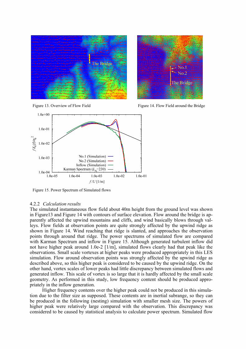
4.2.2 Calculation results The simulated instantaneous flow field about 40m height from the ground level was shown in Figure13 and Figure 14 with contours of surface elevation. Flow around the bridge is ap-parently affected the upwind mountains and cliffs, and wind basically blows through val-leys. Flow fields at observation points are quite strongly affected by the upwind ridge as shown in Figure 14. Wind reaching that ridge is slanted, and approaches the observation points through around that ridge. The power spectrums of simulated flow are compared with Karman Spectrum and inflow in Figure 15. Although generated turbulent inflow did not have higher peak around 1.0e-2 [1/m], simulated flows clearly had that peak like the observations. Small scale vortexes at higher peaks were produced appropriately in this LES simulation. Flow around observation points was strongly affected by the upwind ridge as described above, so this higher peak is considered to be caused by the upwind ridge. On the other hand, vortex scales of lower peaks had little discrepancy between simulated flows and generated inflow. This scale of vortex is so large that it is hardly affected by the small scale geometry. As performed in this study, low frequency content should be produced appro-priately in the inflow generation. Higher frequency contents over the higher peak could not be produced in this simula-tion due to the filter size as supposed. These contents are in inertial subrange, so they can be produced in the following (nesting) simulation with smaller mesh size. The powers of higher peak were relatively large compared with the observation. This discrepancy was considered to be caused by statistical analysis to calculate power spectrum. Simulated flow

Figure 13. Overview of Flow Field Figure 14. Flow Field around the Bridge

Figure 15. Power Spectrum of Simulated flows

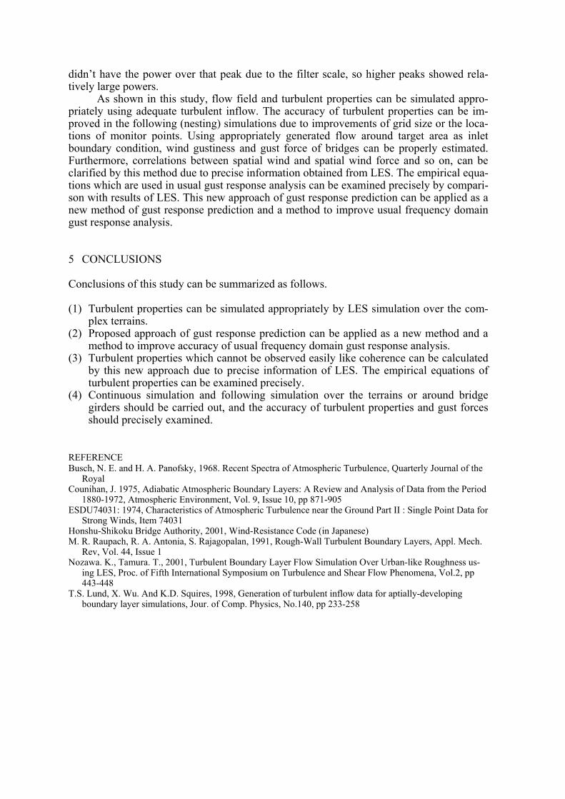
didn’t have the power over that peak due to the filter scale, so higher peaks showed rela-tively large powers.

As shown in this study, flow field and turbulent properties can be simulated appro-priately using adequate turbulent inflow. The accuracy of turbulent properties can be im-proved in the following (nesting) simulations due to improvements of grid size or the loca-tions of monitor points. Using appropriately generated flow around target area as inlet boundary condition, wind gustiness and gust force of bridges can be properly estimated. Furthermore, correlations between spatial wind and spatial wind force and so on, can be clarified by this method due to precise information obtained from LES. The empirical equa-tions which are used in usual gust response analysis can be examined precisely by compari-son with results of LES. This new approach of gust response prediction can be applied as a new method of gust response prediction and a method to improve usual frequency domain gust response analysis.

5 CONCLUSIONS

Conclusions of this study can be summarized as follows.

(1) Turbulent properties can be simulated appropriately by LES simulation over the com-plex terrains.

(2) Proposed approach of gust response prediction can be applied as a new method and a method to improve accuracy of usual frequency domain gust response analysis.

(3) Turbulent properties which cannot be observed easily like coherence can be calculated by this new approach due to precise information of LES. The empirical equations of turbulent properties can be examined precisely.

(4) Continuous simulation and following simulation over the terrains or around bridge girders should be carried out, and the accuracy of turbulent properties and gust forces should precisely examined.

REFERENCE Busch, N. E. and H. A. Panofsky, 1968. Recent Spectra of Atmospheric Turbulence, Quarterly Journal of the

Royal Counihan, J. 1975, Adiabatic Atmospheric Boundary Layers: A Review and Analysis of Data from the Period

1880-1972, Atmospheric Environment, Vol. 9, Issue 10, pp 871-905 ESDU74031: 1974, Characteristics of Atmospheric Turbulence near the Ground Part II : Single Point Data for

Strong Winds, Item 74031 Honshu-Shikoku Bridge Authority, 2001, Wind-Resistance Code (in Japanese) M. R. Raupach, R. A. Antonia, S. Rajagopalan, 1991, Rough-Wall Turbulent Boundary Layers, Appl. Mech.

Rev, Vol. 44, Issue 1 Nozawa. K., Tamura. T., 2001, Turbulent Boundary Layer Flow Simulation Over Urban-like Roughness us-

ing LES, Proc. of Fifth International Symposium on Turbulence and Shear Flow Phenomena, Vol.2, pp 443-448

T.S. Lund, X. Wu. And K.D. Squires, 1998, Generation of turbulent inflow data for aptially-developing boundary layer simulations, Jour. of Comp. Physics, No.140, pp 233-258