Embed Size (px)
Citation preview
Occasional Paper Series Macroprudential stress test of the euro area banking system
Katarzyna Budnik, Mirco Balatti Mozzanica, Ivan Dimitrov, Johannes Groß, Ib Hansen,
Giovanni di Iasio, Michael Kleemann, Francesco Sanna, Andrei Sarychev,
Nadežda Siņenko, Matjaz Volk
No 226 / July 2019
Disclaimer: This paper should not be reported as representing the views of the European Central Bank (ECB). The views expressed are those of the authors and do not necessarily reflect those of the ECB.
ECB Occasional Paper Series No 226 / July 2019 1
Contents
Abstract 3
Executive summary 4
1 Introduction 6
2 Methodology 8
3 Baseline scenario 11
4 Adverse scenario 14
4.1 The risk narrative 14
4.2 Impact on the banking system 16
Box 1 Comparing micro- and macroprudential versions of the euro area stress test 21
Box 2 Comparison with the IMF Euro Area Financial System Stability Assessment of 2018 27
4.3 Augmenting the adverse scenario with a feedback loop 28
5 Discussion of selected results 31
5.1 Solvency: banks deleverage to meet requirements 31
5.2 Legacy assets: balance sheet quality and banks’ vulnerability in the adverse scenario 34
5.3 Vulnerabilities: low profitability and low capital 36
5.4 Foreign lending: a source of cross-country spillovers 37
5.5 Profit distribution: dividend payouts considerably constrained and depressed 38
5.6 Contagion channels 39
6 The role of non-bank financial intermediaries 42
7 Conclusions 48
References 49
Appendices 51
Appendix 1: Implementation of the feedback loop and cure rates 51
Appendix 2: Contagion Model 53

ECB Occasional Paper Series No 226 / July 2019
2
ECB Occasional Paper Series No 226 / July 2019
3
Abstract
This paper presents an approach to a macroprudential stress test for the euro area banking system, comprising the 91 largest euro area credit institutions across 19 countries. The approach involves modelling banks’ reactions to changing economic conditions. It also examines the effects of adverse scenarios on economies and the financial system as a whole by acknowledging a broad set of interactions and interdependencies between banks, other market participants, and the real economy. Our results highlight the importance of the starting level of bank capital, bank asset quality, and banks’ adjustments for the propagation of shocks to the financial sector and real economy.
Keywords: macro stress test, macroprudential policy, banking sector deleveraging, real-financial feedback mechanism
JEL codes: E37, E58, G21, G28
ECB Occasional Paper Series No 226 / July 2019
4
Executive summary
Stress tests are an important tool for assessing banking sector vulnerabilities and resilience. The complexity of financial institutions’ balance sheets and the diversity of their business models make it challenging to correctly identify banks' sensitivities. Stress test exercises illustrate how the banking system would perform under adverse circumstances and provide information about potential capital needs of institutions. As such they have high value in informing regulators and market participants about weak spots in the functioning of financial intermediation.
This paper presents the methodology of a macroprudential stress test of the euro area banking sector. This methodology differs from that of the regular European Union wide stress test led by the European Banking Authority (EBA) in two main respects: (i) the constant balance sheet assumption is relaxed in order to study dynamic adjustments of banks; (ii) it permits the comprehensive modelling of an adverse feedback loop between the banking sector and the real economy. The core of the feedback mechanism is a link between banks’ capitalisation and aggregate credit to the real economy. The purpose of including the feedback loop is to increase awareness of systemic risks that can be triggered by adverse macroeconomic developments. Another difference between the two approaches is that the macroprudential stress test assesses the resilience of the banking system as a whole, while the EBA supervisory exercise is applied to assess the resilience of individual institutions.
To illustrate the proposed methodology we evaluate the performance of the euro area banking sector in 2018-20 under the scenarios of the 2018 EBA supervisory stress test. In the exercise we focus on 91 significant euro area banks. Our results complement the findings of the supervisory stress test and confirm that the euro area banking system is resilient to deep simultaneous recessions in the euro area and global economies combined with large falls in asset prices.
Compared with the results derived under the constant balance sheet assumption, banks’ system-wide capital depletion in the adverse scenario is higher in the macroprudential stress test. When comparing adverse system-wide CET1 capital levels in 2020 against the end of 2017, the macroprudential stress test reveals a €35 billion higher capital depletion then the analogous constant balance sheet exercise for the same sample of banks. However, because of banks’ deleveraging, CET1 ratios are on average higher in the macroprudential stress test.
Compared with the 2018 Financial Sector Assessment Program (FSAP) stress test results, the timing of the impact on bank solvency differs. The FSAP foresees a gradual impact of the adverse scenario on banks’ capital, in contrast to the more frontloaded impact in the macroprudential stress test. The prediction of relatively lower capital ratios by the FSAP is mainly driven by higher severity for certain high-spread economies, and by the less pronounced deleveraging of banks facing strained capital levels.
ECB Occasional Paper Series No 226 / July 2019
5
Banks experiencing a CET1 capital shortfall compared with their capital requirement decrease their lending to a relatively greater degree than do banks with a CET1 surplus. Accordingly, loan growth of a large share of banks in the adverse scenario is negative, especially in the case of non-financial corporations. In the recession, non-performing loan (NPL) ratios double from 4% to 8% up to 2020. The sharpest increase in the ratio is observed for consumer credit. Finally, most banks cut dividends sharply when they face negative net returns.
In addition to the results based on the original adverse scenario, the report introduces an augmented adverse scenario involving a ‘credit crunch’. Excessive bank deleveraging followed by a ‘credit crunch’ could result in additional strain on the macroeconomy and further amplify the severity of the recession. The amplification effect is most likely to arise in banking systems with lower capitalisation. Against this background, the original adverse scenario could be considered a lower bound for the severity of the subsequent recession. In the augmented adverse scenario GDP drops by an additional 1.6% at the euro area level. In the cross-country perspective, the amplification mechanism is more pronounced for those countries that already show relatively low capitalisation of their banking systems at the beginning of the scenario horizon.
Interbank contagion may advance the deterioration of banks’ capital shortfalls. A contagion mechanism related to the direct interconnected-ness between banks could lead to an additional CET1 ratio depletion amounting to 75 basis points by the end of 2020. This estimate involves both solvency and liquidity distress and assumes a default on bilateral exposures and short-term funding withdrawal by those banks experiencing capital shortfalls.
Credit from non-bank financial firms would only partially compensate for the drop in bank loans. When facing a reduction in the supply of bank loans, non-financial corporations (NFCs) will issue more bonds that are mainly acquired by non-banks and other real money investors. However, this will only partially compensate for the reduction in bank loans. Additionally, adverse macroeconomic and market conditions may trigger outflows from investment funds, as well as mutually reinforcing asset fire sales that impact negatively on banks and may further hamper their credit supply.
ECB Occasional Paper Series No 226 / July 2019
6
1 Introduction
Following the last financial crisis with its international dimension, in Europe great hopes have been vested in area-wide stress testing. Since 2011 the European Banking Authority (EBA), in cooperation with the European Systemic Risk Board (ESRB) and the European Central Bank (ECB), has been conducting a European Union (EU)-wide stress test of the banking system. This exercise benefits from the EU-wide coordination of macroeconomic scenarios, methodologies, benchmarks and broad cross-country coverage of all large EU banking institutions. Its methodology includes a range of assumptions, which increases the prudence of the exercise. For instance, the methodology excludes any action that banks may undertake to adjust the size or the composition of their assets and liabilities in response to adverse developments. At the same time, the constant balance sheet assumption rules out credit crunches and feedback from the financial sector to the real economy.
This paper discusses a complementary approach to stress testing where banks are allowed to adjust their balance sheets in response to macroeconomic developments. The core analysis rests on a semi-structural model of the euro area economies and 91 significant euro area banks. We choose to illustrate the approach using the same baseline and adverse scenarios as were used for the 2018 EU-wide exercise. In this setup, we discuss in detail banking sector results. Further, we look at the interactions between banks and the real economy and at how bank responses to stress may lead to additional amplification of initial, especially adverse, shocks. Last, using a set of partial equilibrium models we discuss the implications of contagion between banks and between banks and other financial market participants.
The analyses presented in this paper comprise but are not limited to the evolution of solvency ratios. In line with its macroprudential focus, the paper also discusses banks’ own-fund volumes, credit to the non-financial private sector, and aggregate economic output. The results show that once banks are allowed to adjust their balance sheets in response to adverse shocks, their solvency ratios are likely to remain higher than under the constant balance sheet assumption. However, affected economies may experience deeper contractions in credit, causing further deterioration in output. In order to prevent excessive credit shortages in adverse circumstances, capitalisation of the banking system may consequently need to be further increased.
Such a macroprudential stress test can be particularly relevant for macroprudential authorities. It can achieve one or more of three objectives. First, it may build a complementary metric for judging the resilience of the banking sector. Second, it can encourage banks and regulators to think about the system-wide consequences of banks’ most likely decisions in the situation of stress. And third, it can be used for scenario analysis to assess the reaction of the banking system when considering alternative macroprudential policy paths.
By acknowledging that banks react to market conditions, a macroprudential stress test builds a complementary metric for judging the resilience of the
ECB Occasional Paper Series No 226 / July 2019
7
banking sector. It offers insight into system dynamics under a more ‘realistic’ though often also less prudent set of assumptions compared with constant balance sheet stress tests. In addition, it provides information to policy-makers about: (i) the evolution of the system as a whole including e.g. credit dynamics, and (ii) the strength of the second-round effects, i.e. the intensity of endogenous systemic risks.
By illustrating how banks are likely to adjust in adverse circumstances, it encourages reflection on optimal adaptation strategies. A macroprudential stress test can provide additional information to banks on the impact on the system of single but often correlated decisions. In this role, stress tests constitute a ‘public good’ by providing better information to economic agents and facilitating the fine-tuning of their strategies.
Lastly, a macroprudential stress test can help to select and calibrate macroprudential instruments. The reaction of banks depends on their initial and target levels of capitalisation, with the latter being closely related to the regulatory setup. The outcomes of macroprudential stress tests will help in assessing the appropriateness of already announced capital buffers for the resilience of the banking sector and the supply of credit to the economy. The methodology and supporting analysis allow a quicker reaction of macroprudential authorities in the face of a crisis and facilitate anticipatory setting of macroprudential measures.1
The paper is structured as follows. The next section summarises our modelling approach. Section 3 presents the stress test results in the baseline scenario, while Section 4 lays out the main results for the adverse scenario. All results summarised are based on banks’ reactions to the original adverse scenario included in the 2018 EU-wide stress testing exercise. Section 5 elaborates on selected aspects of the adverse and baseline scenarios along with the macroprudential perspective. It also introduces estimates of the effect of triggering the second-round effects on output and the real economy more broadly. Section 6 discusses the potential role of non-banks in the transmission of the adverse scenario. Section 7 concludes.
1 In a 2015 speech, Vítor Constâncio contrasted the scope of macroprudential stress testing and that of
supervisory stress test exercises along four dimensions: (i) constant versus dynamic balance sheet perspective, (ii) banks’ reactions, (iii) two-way interaction between liquidity and the real economy, and (iv) the interactions between banks and other sectors of the economy.
ECB Occasional Paper Series No 226 / July 2019
8
2 Methodology
The most notable element of our approach is the relaxation of the static balance sheet assumption in order to study the dynamic adjustments of banks and economies. The static balance sheet assumption is an important element of many supervisory stress tests, as it helps to ensure comparability of results across banks. At the same time, it precludes an analysis of banks’ reactions in response to the stress, reactions which are of genuine interest to macroprudential supervision.
The analysis in the next three sections employs a large scale semi-structural model linking macro and bank-level data. The model features a macroeconomic block for the 19 euro area economies and the representation of 91 significant banks2 with their individual balance sheets and profit and loss accounts. The macro block captures dynamic interdependencies of aggregate real and financial variables as well as cross-country spillovers via trade linkages. Banks in the model cover broadly 70% of banking sector assets in the euro area. They are represented with a sufficiently granular sectoral and geographical breakdown of assets and liabilities to reflect the main sources of heterogeneity across banks and their differential sensitivities towards macroeconomic shocks. The liability side distinguishes equity as well as wholesale and retail funding dynamics. For each bank, profitability and capital trends are further broken down into the impact of credit and market risk, net interest income, and dividend payouts.3
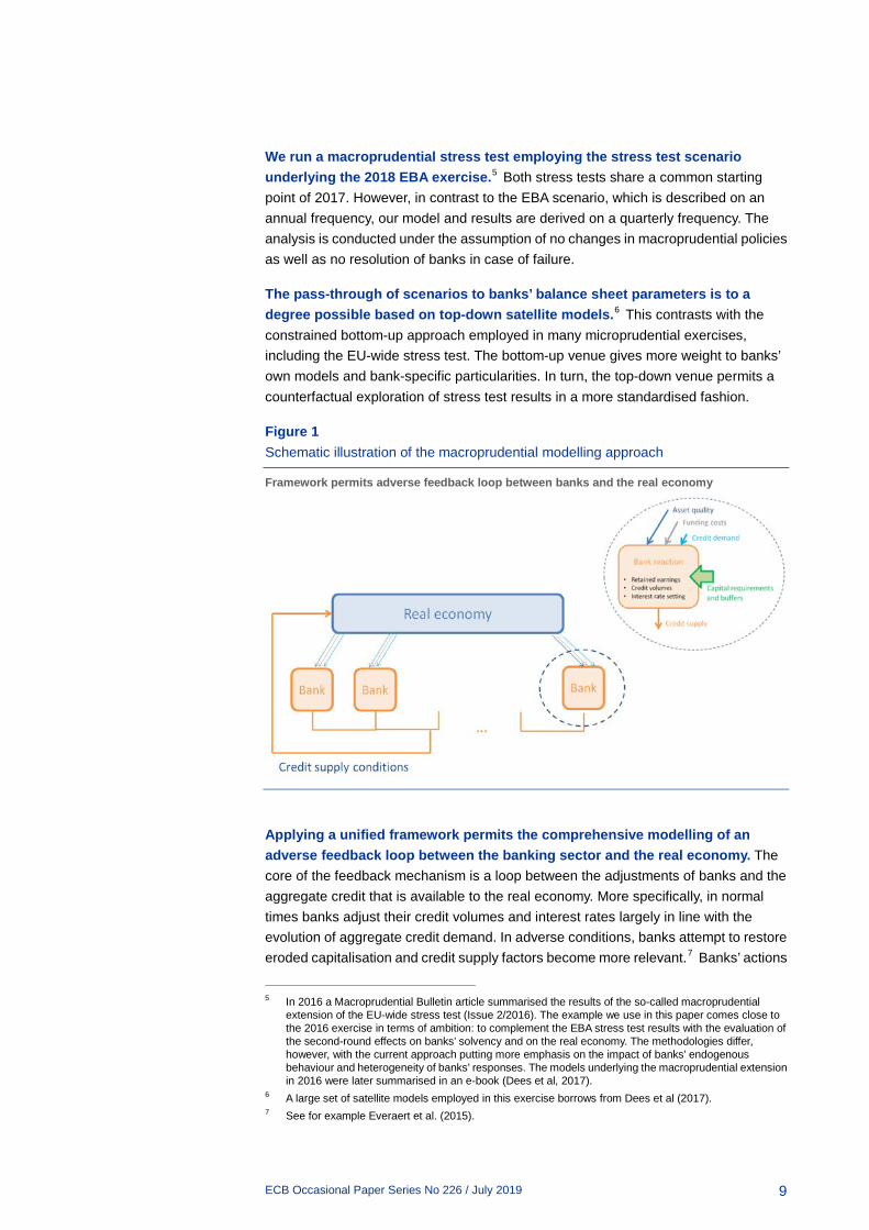
Estimated behavioural relationships govern banks’ behavioural responses to the evolution of loan volumes, loan pricing, funding costs and profit distribution policies (Figure 1). In particular, banks react to changes in general economic conditions and avoid undercutting capital targets set by a combination of regulatory capital minimum requirements and buffers. Evidence suggests that such solvency constraints are enforced not only by the regulator but also by market discipline.4
The model analyses amplification effects through banks’ adjustments in the presence of solvency constraints. In times of stress, solvency thresholds that prompt banks to adjust their balance sheets are likely to lie above regulatory minimum requirements.
2 The sample of banks includes 6 banks headquartered in Austria, 6 in Belgium, 2 in Cyprus, 19 in
Germany, 11 in Spain, 2 in Finland, 10 in France, 4 in Greece, 4 in Ireland, 9 in Italy, 5 in Luxembourg, 2 in Malta, 6 in the Netherlands, 2 in Portugal and 3 in Slovenia.
3 The detailed description of the model is included in “Banking euro area stress test model”, by Budnik, K., Balatti, M, Dimitrov, I., Gross, J, Kleemann, M., Reichenbachas, T., Sanna, F., Sarychev, A., Sinienko, N., Volk, M., to be published still in 2019. The manuscript is available from the authors upon request.
4 See for example Estrella (2004), Gropp and Heider (2010), Cummings and Durrani (2016).
ECB Occasional Paper Series No 226 / July 2019
9
We run a macroprudential stress test employing the stress test scenario underlying the 2018 EBA exercise.5 Both stress tests share a common starting point of 2017. However, in contrast to the EBA scenario, which is described on an annual frequency, our model and results are derived on a quarterly frequency. The analysis is conducted under the assumption of no changes in macroprudential policies as well as no resolution of banks in case of failure.
The pass-through of scenarios to banks’ balance sheet parameters is to a degree possible based on top-down satellite models.6 This contrasts with the constrained bottom-up approach employed in many microprudential exercises, including the EU-wide stress test. The bottom-up venue gives more weight to banks’ own models and bank-specific particularities. In turn, the top-down venue permits a counterfactual exploration of stress test results in a more standardised fashion.
Figure 1 Schematic illustration of the macroprudential modelling approach
Framework permits adverse feedback loop between banks and the real economy
Applying a unified framework permits the comprehensive modelling of an adverse feedback loop between the banking sector and the real economy. The core of the feedback mechanism is a loop between the adjustments of banks and the aggregate credit that is available to the real economy. More specifically, in normal times banks adjust their credit volumes and interest rates largely in line with the evolution of aggregate credit demand. In adverse conditions, banks attempt to restore eroded capitalisation and credit supply factors become more relevant.7 Banks’ actions
5 In 2016 a Macroprudential Bulletin article summarised the results of the so-called macroprudential
extension of the EU-wide stress test (Issue 2/2016). The example we use in this paper comes close to the 2016 exercise in terms of ambition: to complement the EBA stress test results with the evaluation of the second-round effects on banks’ solvency and on the real economy. The methodologies differ, however, with the current approach putting more emphasis on the impact of banks’ endogenous behaviour and heterogeneity of banks’ responses. The models underlying the macroprudential extension in 2016 were later summarised in an e-book (Dees et al, 2017).
6 A large set of satellite models employed in this exercise borrows from Dees et al (2017). 7 See for example Everaert et al. (2015).
ECB Occasional Paper Series No 226 / July 2019
10
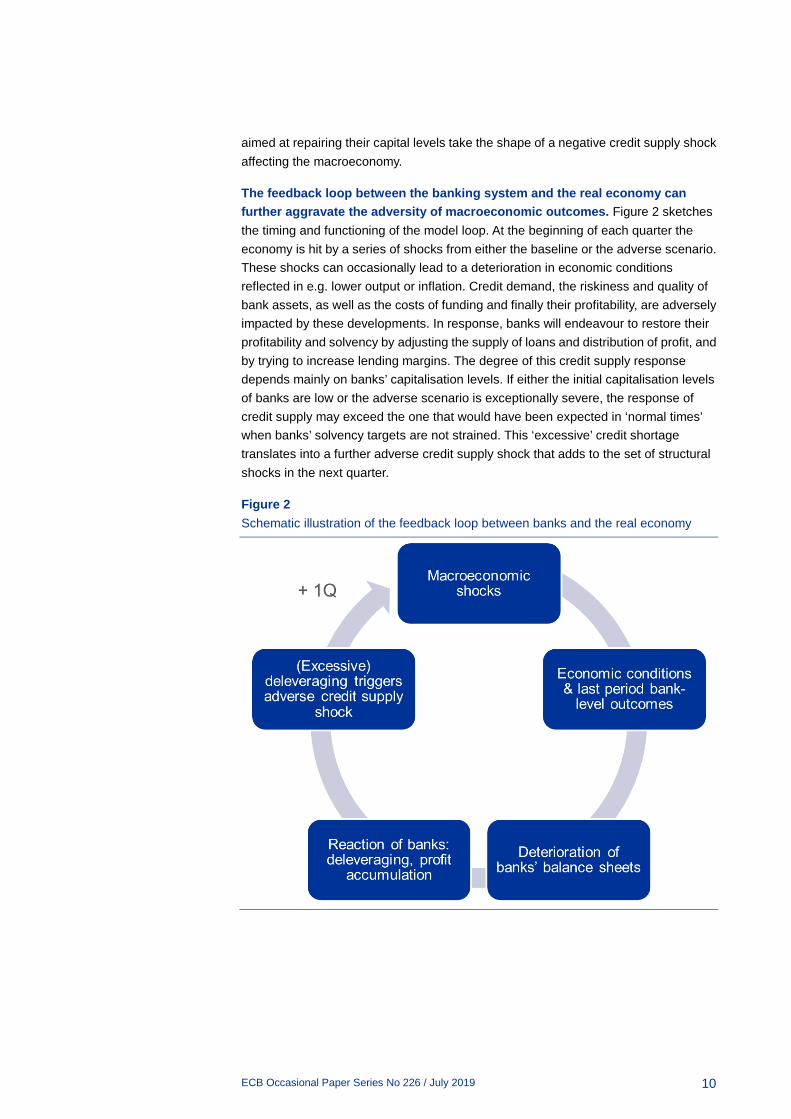
aimed at repairing their capital levels take the shape of a negative credit supply shock affecting the macroeconomy.
The feedback loop between the banking system and the real economy can further aggravate the adversity of macroeconomic outcomes. Figure 2 sketches the timing and functioning of the model loop. At the beginning of each quarter the economy is hit by a series of shocks from either the baseline or the adverse scenario. These shocks can occasionally lead to a deterioration in economic conditions reflected in e.g. lower output or inflation. Credit demand, the riskiness and quality of bank assets, as well as the costs of funding and finally their profitability, are adversely impacted by these developments. In response, banks will endeavour to restore their profitability and solvency by adjusting the supply of loans and distribution of profit, and by trying to increase lending margins. The degree of this credit supply response depends mainly on banks’ capitalisation levels. If either the initial capitalisation levels of banks are low or the adverse scenario is exceptionally severe, the response of credit supply may exceed the one that would have been expected in ‘normal times’ when banks’ solvency targets are not strained. This ‘excessive’ credit shortage translates into a further adverse credit supply shock that adds to the set of structural shocks in the next quarter.
Figure 2 Schematic illustration of the feedback loop between banks and the real economy
ECB Occasional Paper Series No 226 / July 2019
11
3 Baseline scenario
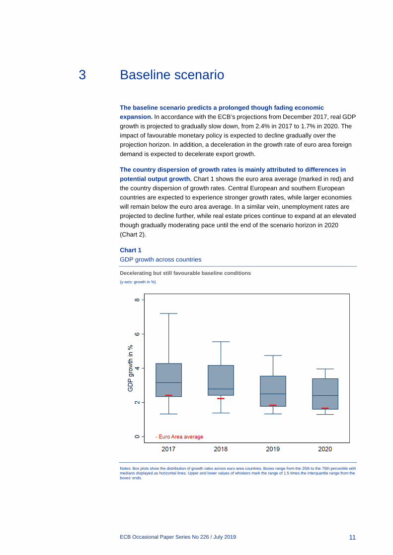
The baseline scenario predicts a prolonged though fading economic expansion. In accordance with the ECB’s projections from December 2017, real GDP growth is projected to gradually slow down, from 2.4% in 2017 to 1.7% in 2020. The impact of favourable monetary policy is expected to decline gradually over the projection horizon. In addition, a deceleration in the growth rate of euro area foreign demand is expected to decelerate export growth.
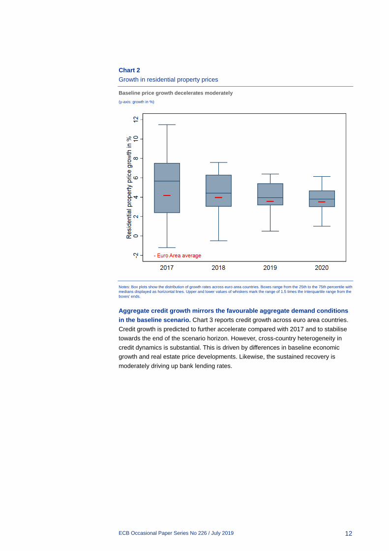
The country dispersion of growth rates is mainly attributed to differences in potential output growth. Chart 1 shows the euro area average (marked in red) and the country dispersion of growth rates. Central European and southern European countries are expected to experience stronger growth rates, while larger economies will remain below the euro area average. In a similar vein, unemployment rates are projected to decline further, while real estate prices continue to expand at an elevated though gradually moderating pace until the end of the scenario horizon in 2020 (Chart 2).
Chart 1 GDP growth across countries
Decelerating but still favourable baseline conditions (y-axis: growth in %)
Notes: Box plots show the distribution of growth rates across euro area countries. Boxes range from the 25th to the 75th percentile with medians displayed as horizontal lines. Upper and lower values of whiskers mark the range of 1.5 times the interquartile range from the boxes’ ends.
ECB Occasional Paper Series No 226 / July 2019
12
Chart 2 Growth in residential property prices
Baseline price growth decelerates moderately (y-axis: growth in %)
Notes: Box plots show the distribution of growth rates across euro area countries. Boxes range from the 25th to the 75th percentile with medians displayed as horizontal lines. Upper and lower values of whiskers mark the range of 1.5 times the interquartile range from the boxes’ ends.
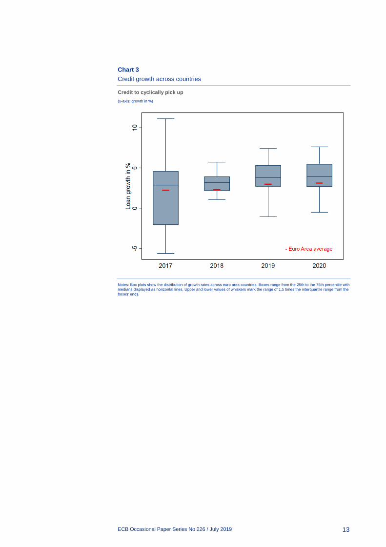
Aggregate credit growth mirrors the favourable aggregate demand conditions in the baseline scenario. Chart 3 reports credit growth across euro area countries. Credit growth is predicted to further accelerate compared with 2017 and to stabilise towards the end of the scenario horizon. However, cross-country heterogeneity in credit dynamics is substantial. This is driven by differences in baseline economic growth and real estate price developments. Likewise, the sustained recovery is moderately driving up bank lending rates.
ECB Occasional Paper Series No 226 / July 2019
13
Chart 3 Credit growth across countries
Credit to cyclically pick up (y-axis: growth in %)
Notes: Box plots show the distribution of growth rates across euro area countries. Boxes range from the 25th to the 75th percentile with medians displayed as horizontal lines. Upper and lower values of whiskers mark the range of 1.5 times the interquartile range from the boxes’ ends.
ECB Occasional Paper Series No 226 / July 2019
14
4 Adverse scenario
4.1 The risk narrative
The adverse scenario assumes the materialisation of four financial stability risks, which the European Systemic Risk Board has identified as representing the most material threats to the euro area banking sector. The first of these risks is an abrupt and sizeable repricing of risk premia in global financial markets. Its materialisation spills over to the European countries though financial markets and foreign demand. The second risk relates to the decline in economic activity in the euro area, affecting in particular countries facing structural challenges in their banking sector. The third risk concerns increased political uncertainty and a resurgence of public and private debt sustainability concerns amid a potential repricing of risk premia. Fourth, liquidity risks in the non-bank financial sector materialise and spill over into the broader financial system.
The materialisation of the four risks is expected to result in a severe recession. The strongest negative impact on economic activity is expected in 2018 and 2019, with annual GDP growth rates of -0.9% and -2% respectively. This is 3.1 percentage points and 3.9 percentage points below the baseline projections. In 2020 the euro area is predicted to experience positive growth at a rate of 0.5% again, which still ranges 1.2 percentage points below baseline. Overall, the adverse scenario underlying the EBA exercise implies a deviation of euro area GDP from its baseline level by 7.8% in 2020 (Chart 4). Putting this in perspective, the cumulative GDP drop between the beginning and the trough of this recession would be 4.1% of GDP, which is still less severe than in the last recession, when it was equal to 6.1%.8
In the scenario, negative domestic demand shocks reflect the impacts of the systemic risks associated with the euro area’s weak nominal growth, structural challenges, and debt sustainability concerns.9 Chart 4 presents a decomposition of the difference between the adverse and the baseline scenarios into the effect of economic shocks reflecting the narrative underlying the adverse scenario. This model-based decomposition serves two aims. First, it illustrates relative impacts of several shocks to the build-up of the adverse scenario. Second, it shows the evolution of the economy in the adverse scenario in the absence of an amplification effect stemming from non-linear response of banks’ credit supply.
8 A detailed description of the adverse scenario underlying the EBA’s EU-wide stress test exercise in 2018,
including details of the methodology, is available here. 9 The baseline and adverse scenarios assume the same path of monetary policy interest rates in line with
market expectations. All other things being equal, this amplifies the gap between the baseline and adverse forecasts of growth.

ECB Occasional Paper Series No 226 / July 2019
15
Chart 4 Adverse scenario impact on GDP
Real and financial risks from the global economy matter (y-axis: deviation from baseline in %)
Another factor contributing to the reduction in GDP is the evolution of aggregate foreign demand. This derives from the global repricing of risk premia and the consecutive slowdown in advanced economies and global trade.
House price shocks capture an abrupt reversal of price trends in overheating real estate markets and contribute to the adverse real estate price developments. These two risks trigger an abrupt fall in residential real estate prices, which decrease by 25% to the end of the scenario horizon (Chart 5).
Chart 5 Adverse scenario impact on house prices
The scenario foresees a sudden and substantial drop (y-axis: deviation from baseline in %)
-8
-7
-6
-5
-4
-3
-2
-1
0
Q1 Q2 Q3 Q4 Q1 Q2 Q3 Q4 Q1 Q2 Q3 Q4
2018 2019 2020
Aggregated demand shockAggregated supply shockHousing price shock
Equity price shockForeign demand shock
-30
-25
-20
-15
-10
-5
0
Q1 Q2 Q3 Q4 Q1 Q2 Q3 Q4 Q1 Q2 Q3 Q4
2018 2019 2020
Aggregated demand shockAggregated supply shockHousing price shock
Equity price shockForeign demand shock
ECB Occasional Paper Series No 226 / July 2019
16
Last, equity price shocks reflect direct spillover from financial markets affected by the global repricing of risk premia. They contribute to a general deterioration in asset prices, and more specifically to a sharp decline in euro area equity price indices, by 31%.
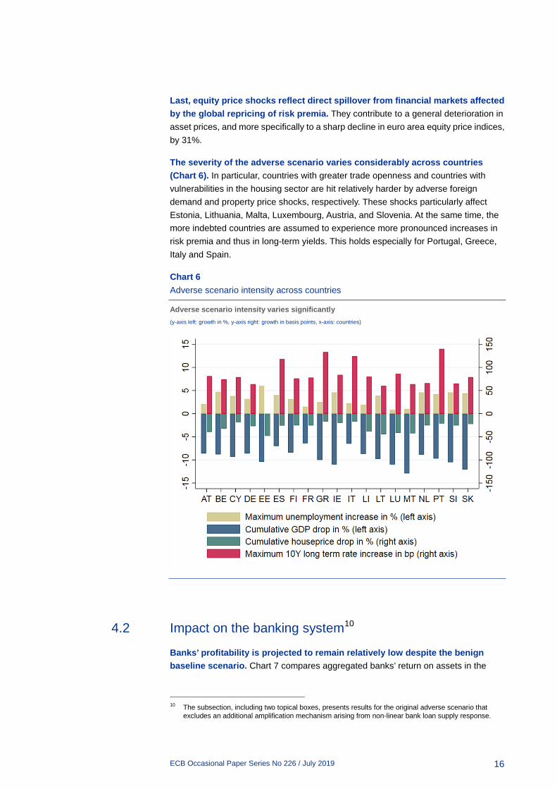
The severity of the adverse scenario varies considerably across countries (Chart 6). In particular, countries with greater trade openness and countries with vulnerabilities in the housing sector are hit relatively harder by adverse foreign demand and property price shocks, respectively. These shocks particularly affect Estonia, Lithuania, Malta, Luxembourg, Austria, and Slovenia. At the same time, the more indebted countries are assumed to experience more pronounced increases in risk premia and thus in long-term yields. This holds especially for Portugal, Greece, Italy and Spain.
Chart 6 Adverse scenario intensity across countries
Adverse scenario intensity varies significantly (y-axis left: growth in %, y-axis right: growth in basis points, x-axis: countries)
4.2 Impact on the banking system10
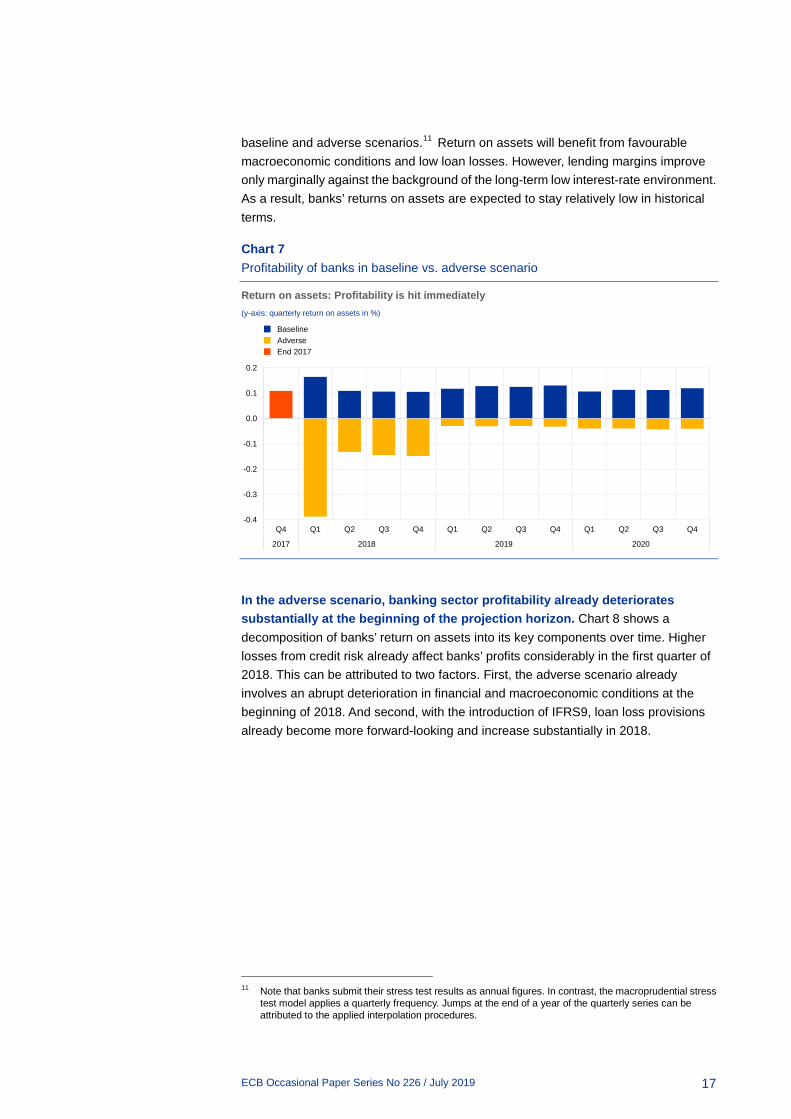
Banks’ profitability is projected to remain relatively low despite the benign baseline scenario. Chart 7 compares aggregated banks’ return on assets in the
10 The subsection, including two topical boxes, presents results for the original adverse scenario that
excludes an additional amplification mechanism arising from non-linear bank loan supply response.
ECB Occasional Paper Series No 226 / July 2019
17
baseline and adverse scenarios.11 Return on assets will benefit from favourable macroeconomic conditions and low loan losses. However, lending margins improve only marginally against the background of the long-term low interest-rate environment. As a result, banks’ returns on assets are expected to stay relatively low in historical terms.
Chart 7 Profitability of banks in baseline vs. adverse scenario
Return on assets: Profitability is hit immediately (y-axis: quarterly return on assets in %)
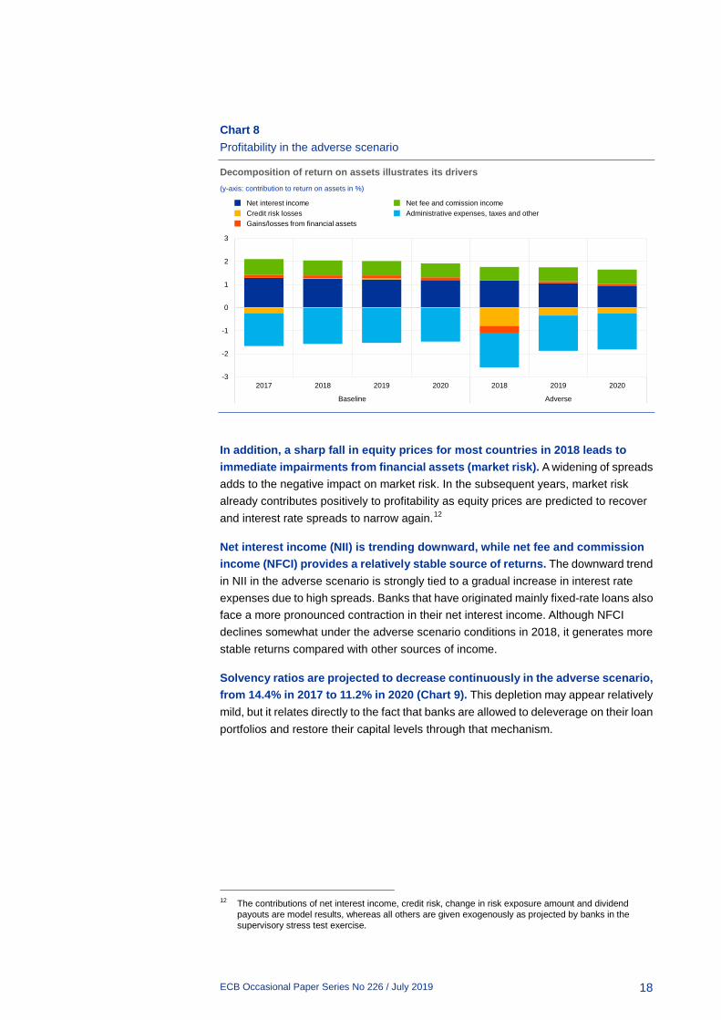
In the adverse scenario, banking sector profitability already deteriorates substantially at the beginning of the projection horizon. Chart 8 shows a decomposition of banks’ return on assets into its key components over time. Higher losses from credit risk already affect banks’ profits considerably in the first quarter of 2018. This can be attributed to two factors. First, the adverse scenario already involves an abrupt deterioration in financial and macroeconomic conditions at the beginning of 2018. And second, with the introduction of IFRS9, loan loss provisions already become more forward-looking and increase substantially in 2018.
11 Note that banks submit their stress test results as annual figures. In contrast, the macroprudential stress
test model applies a quarterly frequency. Jumps at the end of a year of the quarterly series can be attributed to the applied interpolation procedures.
-0.4
-0.3
-0.2
-0.1
0.0
0.1
0.2
Q4 Q1 Q2 Q3 Q4 Q1 Q2 Q3 Q4 Q1 Q2 Q3 Q4
2017 2018 2019 2020
BaselineAdverseEnd 2017
ECB Occasional Paper Series No 226 / July 2019
18
Chart 8 Profitability in the adverse scenario
Decomposition of return on assets illustrates its drivers (y-axis: contribution to return on assets in %)
In addition, a sharp fall in equity prices for most countries in 2018 leads to immediate impairments from financial assets (market risk). A widening of spreads adds to the negative impact on market risk. In the subsequent years, market risk already contributes positively to profitability as equity prices are predicted to recover and interest rate spreads to narrow again.12
Net interest income (NII) is trending downward, while net fee and commission income (NFCI) provides a relatively stable source of returns. The downward trend in NII in the adverse scenario is strongly tied to a gradual increase in interest rate expenses due to high spreads. Banks that have originated mainly fixed-rate loans also face a more pronounced contraction in their net interest income. Although NFCI declines somewhat under the adverse scenario conditions in 2018, it generates more stable returns compared with other sources of income.
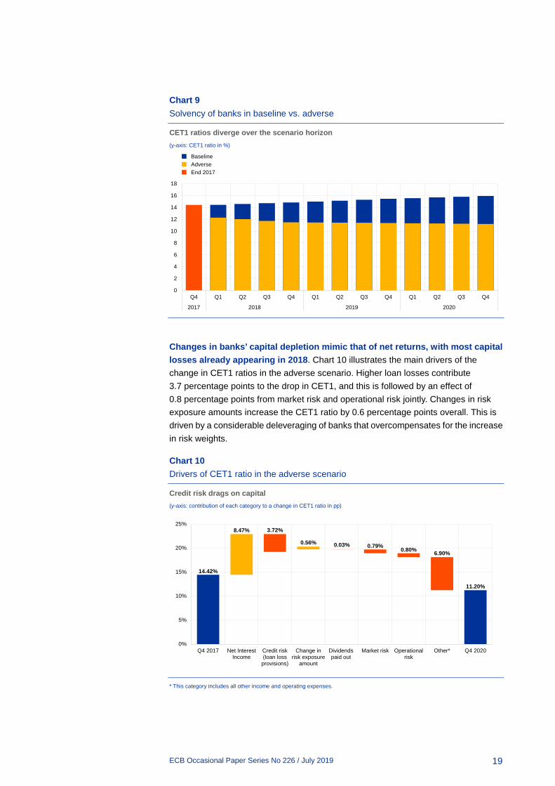
Solvency ratios are projected to decrease continuously in the adverse scenario, from 14.4% in 2017 to 11.2% in 2020 (Chart 9). This depletion may appear relatively mild, but it relates directly to the fact that banks are allowed to deleverage on their loan portfolios and restore their capital levels through that mechanism.
12 The contributions of net interest income, credit risk, change in risk exposure amount and dividend
payouts are model results, whereas all others are given exogenously as projected by banks in the supervisory stress test exercise.
-3
-2
-1
0
1
2
3
2017 2018 2019 2020 2018 2019 2020
Baseline Adverse
Net interest incomeCredit risk lossesGains/losses from financial assets
Net fee and comission incomeAdministrative expenses, taxes and other
ECB Occasional Paper Series No 226 / July 2019
19
Chart 9 Solvency of banks in baseline vs. adverse
CET1 ratios diverge over the scenario horizon (y-axis: CET1 ratio in %)
Changes in banks’ capital depletion mimic that of net returns, with most capital losses already appearing in 2018. Chart 10 illustrates the main drivers of the change in CET1 ratios in the adverse scenario. Higher loan losses contribute 3.7 percentage points to the drop in CET1, and this is followed by an effect of 0.8 percentage points from market risk and operational risk jointly. Changes in risk exposure amounts increase the CET1 ratio by 0.6 percentage points overall. This is driven by a considerable deleveraging of banks that overcompensates for the increase in risk weights.
Chart 10 Drivers of CET1 ratio in the adverse scenario
Credit risk drags on capital (y-axis: contribution of each category to a change in CET1 ratio in pp)
* This category includes all other income and operating expenses.
0
2
4
6
8
10
12
14
16
18
Q4 Q1 Q2 Q3 Q4 Q1 Q2 Q3 Q4 Q1 Q2 Q3 Q4
2017 2018 2019 2020
BaselineAdverseEnd 2017
14.42%
8.47% 3.72%
0.56% 0.03% 0.79% 0.80% 6.90%
11.20%
0%
5%
10%
15%
20%
25%
Q4 2017 Net InterestIncome
Credit risk(loan lossprovisions)
Change inrisk exposure
amount
Dividendspaid out
Market risk Operationalrisk
Other* Q4 2020
ECB Occasional Paper Series No 226 / July 2019
20
Considering banking system-wide capital in 2020, regulatory capital (CET1) decreases by €266 billion relative to 2017 or €457 billion relative to the baseline scenario.
Banks’ loan volumes respond endogenously to the scenario conditions in the macroprudential stress test. Accordingly, lending to the non-financial private sector tightens sharply in the adverse scenario. At the end of the scenario horizon, in 2020, euro area wide credit volumes would be expected to have contracted by 11%.13 This is a considerable contraction compared with an expected increase in the volume of loans of 9% in the baseline.
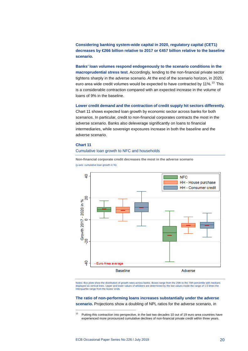
Lower credit demand and the contraction of credit supply hit sectors differently. Chart 11 shows expected loan growth by economic sector across banks for both scenarios. In particular, credit to non-financial corporates contracts the most in the adverse scenario. Banks also deleverage significantly on loans to financial intermediaries, while sovereign exposures increase in both the baseline and the adverse scenario.
Chart 11 Cumulative loan growth to NFC and households
Non-financial corporate credit decreases the most in the adverse scenario (y-axis: cumulative loan growth in %)
Notes: Box plots show the distribution of growth rates across banks. Boxes range from the 25th to the 75th percentile with medians displayed as vertical lines. Upper and lower values of whiskers are determined by the last values inside the range of 1.5 times the interquartile range from the boxes’ ends.
The ratio of non-performing loans increases substantially under the adverse scenario. Projections show a doubling of NPL ratios for the adverse scenario, in 13 Putting this contraction into perspective, in the last two decades 10 out of 19 euro area countries have
experienced more pronounced cumulative declines of non-financial private credit within three years.
ECB Occasional Paper Series No 226 / July 2019
21
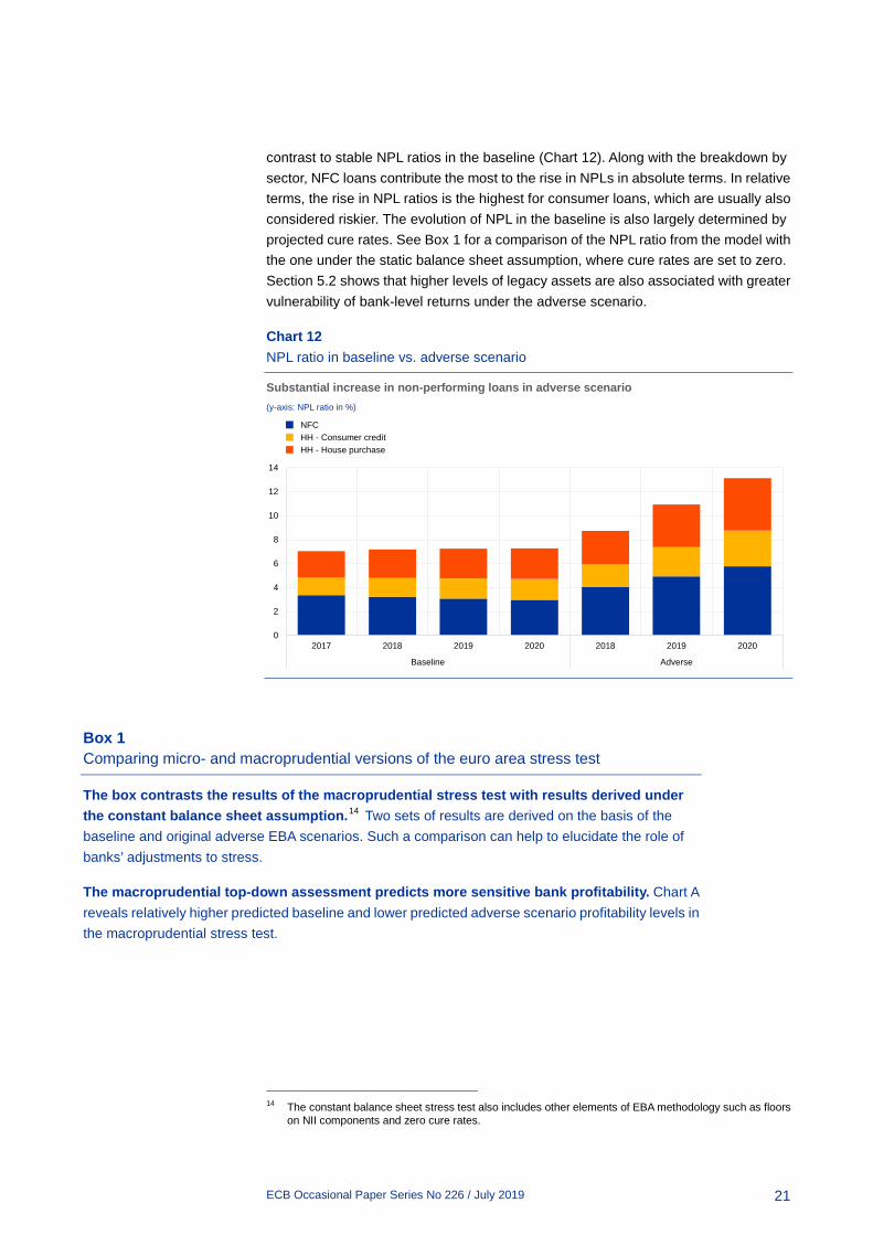
contrast to stable NPL ratios in the baseline (Chart 12). Along with the breakdown by sector, NFC loans contribute the most to the rise in NPLs in absolute terms. In relative terms, the rise in NPL ratios is the highest for consumer loans, which are usually also considered riskier. The evolution of NPL in the baseline is also largely determined by projected cure rates. See Box 1 for a comparison of the NPL ratio from the model with the one under the static balance sheet assumption, where cure rates are set to zero. Section 5.2 shows that higher levels of legacy assets are also associated with greater vulnerability of bank-level returns under the adverse scenario.
Chart 12 NPL ratio in baseline vs. adverse scenario
Substantial increase in non-performing loans in adverse scenario (y-axis: NPL ratio in %)
Box 1 Comparing micro- and macroprudential versions of the euro area stress test
The box contrasts the results of the macroprudential stress test with results derived under the constant balance sheet assumption.14 Two sets of results are derived on the basis of the baseline and original adverse EBA scenarios. Such a comparison can help to elucidate the role of banks’ adjustments to stress.
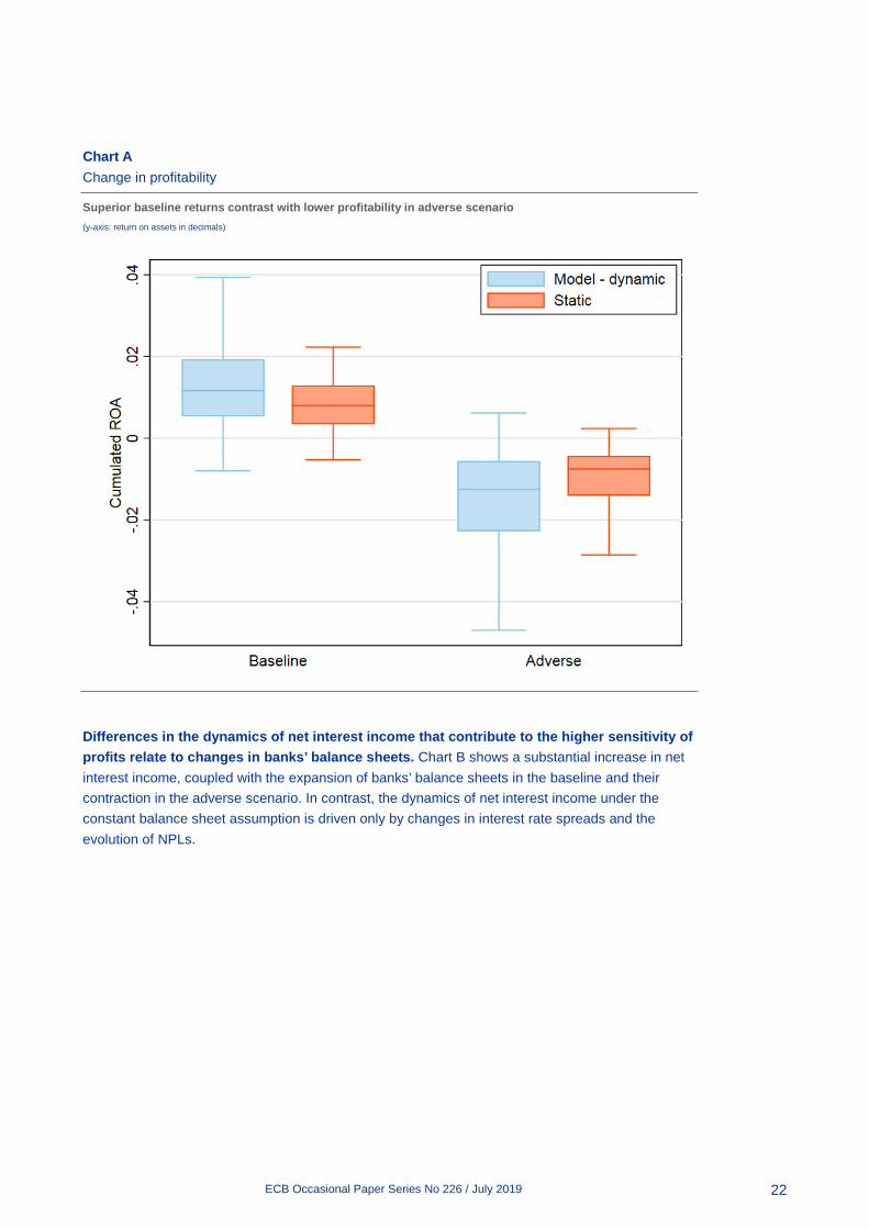
The macroprudential top-down assessment predicts more sensitive bank profitability. Chart A reveals relatively higher predicted baseline and lower predicted adverse scenario profitability levels in the macroprudential stress test.
14 The constant balance sheet stress test also includes other elements of EBA methodology such as floors
on NII components and zero cure rates.
0
2
4
6
8
10
12
14
2017 2018 2019 2020 2018 2019 2020
Baseline Adverse
NFCHH - Consumer creditHH - House purchase
ECB Occasional Paper Series No 226 / July 2019
22
Chart A Change in profitability
Superior baseline returns contrast with lower profitability in adverse scenario (y-axis: return on assets in decimals)
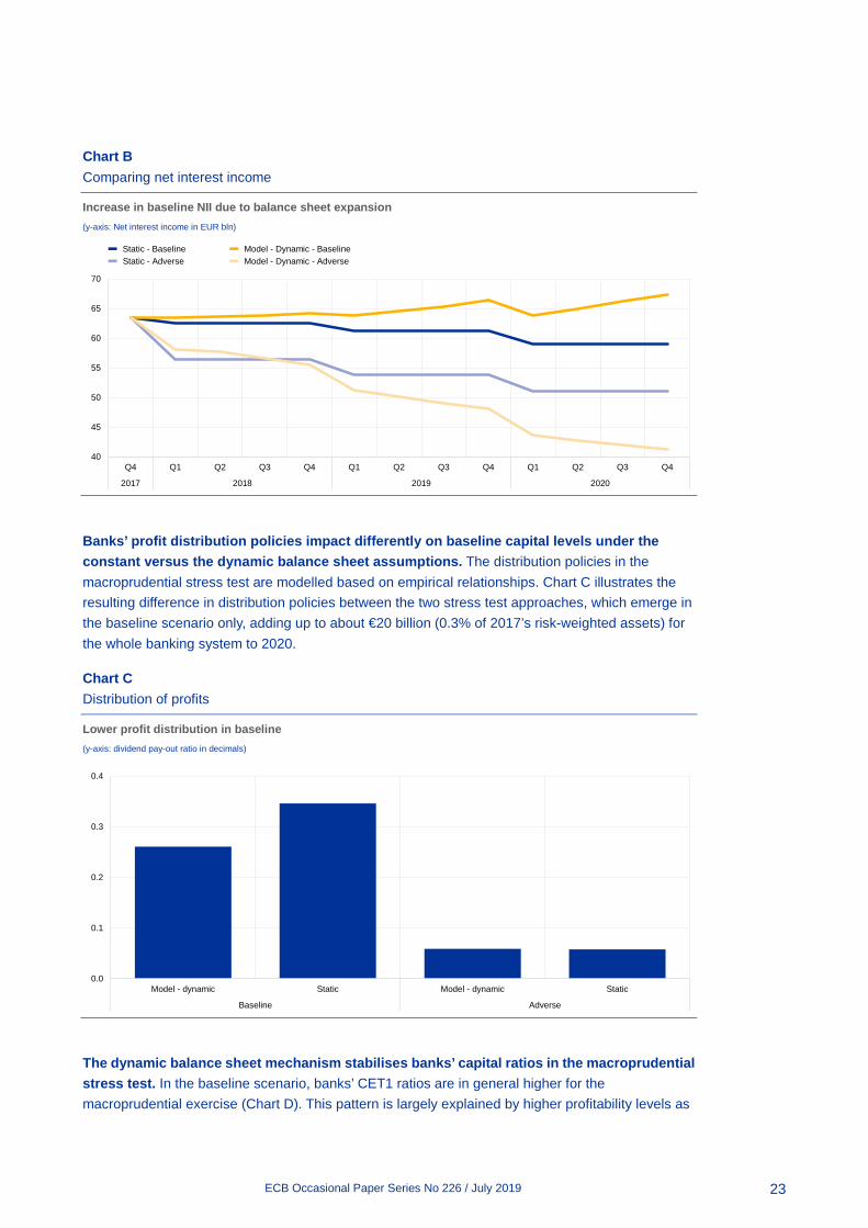
Differences in the dynamics of net interest income that contribute to the higher sensitivity of profits relate to changes in banks’ balance sheets. Chart B shows a substantial increase in net interest income, coupled with the expansion of banks’ balance sheets in the baseline and their contraction in the adverse scenario. In contrast, the dynamics of net interest income under the constant balance sheet assumption is driven only by changes in interest rate spreads and the evolution of NPLs.
ECB Occasional Paper Series No 226 / July 2019
23
Chart B Comparing net interest income
Increase in baseline NII due to balance sheet expansion (y-axis: Net interest income in EUR bln)
Banks’ profit distribution policies impact differently on baseline capital levels under the constant versus the dynamic balance sheet assumptions. The distribution policies in the macroprudential stress test are modelled based on empirical relationships. Chart C illustrates the resulting difference in distribution policies between the two stress test approaches, which emerge in the baseline scenario only, adding up to about €20 billion (0.3% of 2017’s risk-weighted assets) for the whole banking system to 2020.
Chart C Distribution of profits
Lower profit distribution in baseline (y-axis: dividend pay-out ratio in decimals)
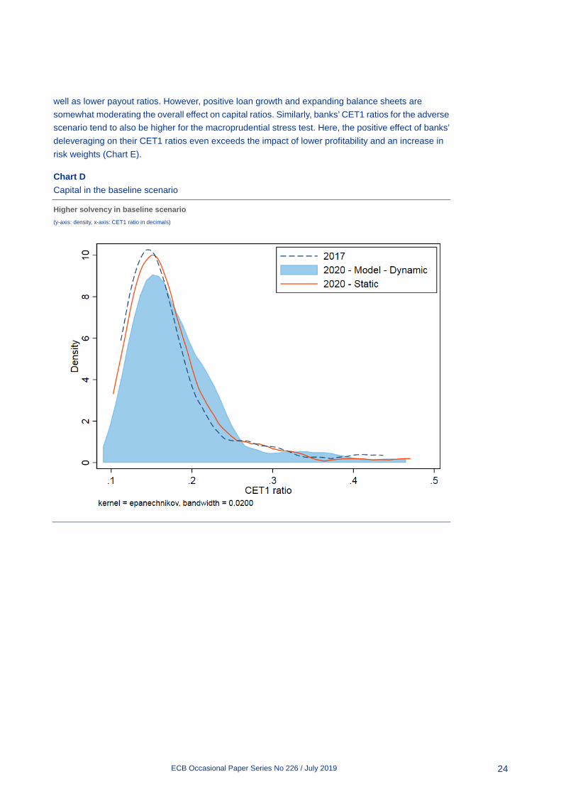
The dynamic balance sheet mechanism stabilises banks’ capital ratios in the macroprudential stress test. In the baseline scenario, banks’ CET1 ratios are in general higher for the macroprudential exercise (Chart D). This pattern is largely explained by higher profitability levels as
40
45
50
55
60
65
70
Q4 Q1 Q2 Q3 Q4 Q1 Q2 Q3 Q4 Q1 Q2 Q3 Q4
2017 2018 2019 2020
Static - BaselineStatic - Adverse
Model - Dynamic - BaselineModel - Dynamic - Adverse
0.0
0.1
0.2
0.3
0.4
Model - dynamic Static Model - dynamic Static
Baseline Adverse
ECB Occasional Paper Series No 226 / July 2019
24
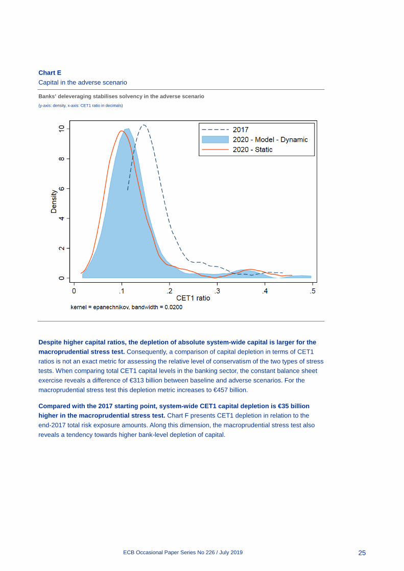
well as lower payout ratios. However, positive loan growth and expanding balance sheets are somewhat moderating the overall effect on capital ratios. Similarly, banks’ CET1 ratios for the adverse scenario tend to also be higher for the macroprudential stress test. Here, the positive effect of banks’ deleveraging on their CET1 ratios even exceeds the impact of lower profitability and an increase in risk weights (Chart E).
Chart D Capital in the baseline scenario
Higher solvency in baseline scenario (y-axis: density, x-axis: CET1 ratio in decimals)
ECB Occasional Paper Series No 226 / July 2019
25
Chart E Capital in the adverse scenario
Banks’ deleveraging stabilises solvency in the adverse scenario (y-axis: density, x-axis: CET1 ratio in decimals)
Despite higher capital ratios, the depletion of absolute system-wide capital is larger for the macroprudential stress test. Consequently, a comparison of capital depletion in terms of CET1 ratios is not an exact metric for assessing the relative level of conservatism of the two types of stress tests. When comparing total CET1 capital levels in the banking sector, the constant balance sheet exercise reveals a difference of €313 billion between baseline and adverse scenarios. For the macroprudential stress test this depletion metric increases to €457 billion.
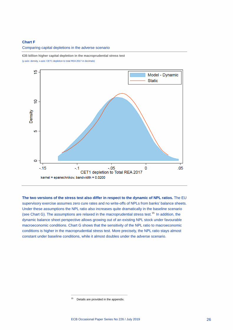
Compared with the 2017 starting point, system-wide CET1 capital depletion is €35 billion higher in the macroprudential stress test. Chart F presents CET1 depletion in relation to the end-2017 total risk exposure amounts. Along this dimension, the macroprudential stress test also reveals a tendency towards higher bank-level depletion of capital.
ECB Occasional Paper Series No 226 / July 2019
26
Chart F Comparing capital depletions in the adverse scenario
€35 billion higher capital depletion in the macroprudential stress test (y-axis: density, x-axis: CET1 depletion to total REA 2017 in decimals)
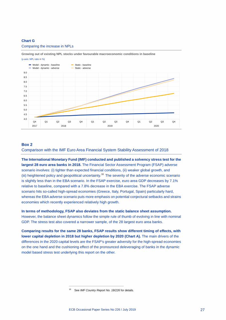
The two versions of the stress test also differ in respect to the dynamic of NPL ratios. The EU supervisory exercise assumes zero cure rates and no write-offs of NPLs from banks’ balance sheets. Under these assumptions the NPL ratio also increases quite dramatically in the baseline scenario (see Chart G). The assumptions are relaxed in the macroprudential stress test.15 In addition, the dynamic balance sheet perspective allows growing out of an existing NPL stock under favourable macroeconomic conditions. Chart G shows that the sensitivity of the NPL ratio to macroeconomic conditions is higher in the macroprudential stress test. More precisely, the NPL ratio stays almost constant under baseline conditions, while it almost doubles under the adverse scenario.
15 Details are provided in the appendix.
ECB Occasional Paper Series No 226 / July 2019
27
Chart G Comparing the increase in NPLs
Growing out of existing NPL stocks under favourable macroeconomic conditions in baseline (y-axis: NPL ratio in %)
Box 2 Comparison with the IMF Euro Area Financial System Stability Assessment of 2018
The International Monetary Fund (IMF) conducted and published a solvency stress test for the largest 28 euro area banks in 2018. The Financial Sector Assessment Program (FSAP) adverse scenario involves: (i) tighter than expected financial conditions, (ii) weaker global growth, and (iii) heightened policy and geopolitical uncertainty.16 The severity of the adverse economic scenario is slightly less than in the EBA scenario. In the FSAP exercise, euro area GDP decreases by 7.1% relative to baseline, compared with a 7.8% decrease in the EBA exercise. The FSAP adverse scenario hits so-called high-spread economies (Greece, Italy, Portugal, Spain) particularly hard, whereas the EBA adverse scenario puts more emphasis on potential conjectural setbacks and strains economies which recently experienced relatively high growth.
In terms of methodology, FSAP also deviates from the static balance sheet assumption. However, the balance sheet dynamics follow the simple rule of thumb of evolving in line with nominal GDP. The stress test also covered a narrower sample, of the 28 largest euro area banks.
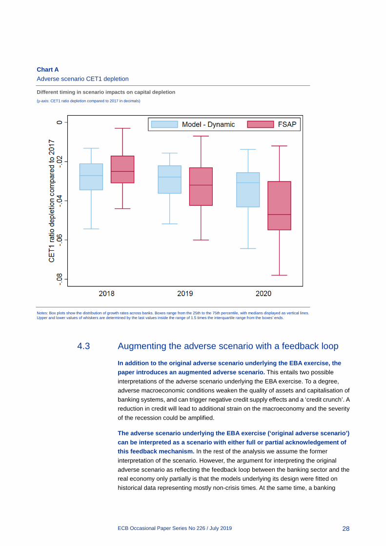
Comparing results for the same 28 banks, FSAP results show different timing of effects, with lower capital depletion in 2018 but higher depletion by 2020 (Chart A). The main drivers of the differences in the 2020 capital levels are the FSAP’s greater adversity for the high-spread economies on the one hand and the cushioning effect of the pronounced deleveraging of banks in the dynamic model based stress test underlying this report on the other.
16 See IMF Country Report No. 18/226 for details.
4.0
4.5
5.0
5.5
6.0
6.5
7.0
7.5
8.0
8.5
9.0
Q4 Q1 Q2 Q3 Q4 Q1 Q2 Q3 Q4 Q1 Q2 Q3 Q4
2017 2018 2019 2020
Model - dynamic - baselineModel - dynamic - adverse
Static - baselineStatic - adverse
ECB Occasional Paper Series No 226 / July 2019
28
Chart A Adverse scenario CET1 depletion
Different timing in scenario impacts on capital depletion (y-axis: CET1 ratio depletion compared to 2017 in decimals)
Notes: Box plots show the distribution of growth rates across banks. Boxes range from the 25th to the 75th percentile, with medians displayed as vertical lines. Upper and lower values of whiskers are determined by the last values inside the range of 1.5 times the interquartile range from the boxes’ ends.
4.3 Augmenting the adverse scenario with a feedback loop
In addition to the original adverse scenario underlying the EBA exercise, the paper introduces an augmented adverse scenario. This entails two possible interpretations of the adverse scenario underlying the EBA exercise. To a degree, adverse macroeconomic conditions weaken the quality of assets and capitalisation of banking systems, and can trigger negative credit supply effects and a ‘credit crunch’. A reduction in credit will lead to additional strain on the macroeconomy and the severity of the recession could be amplified.
The adverse scenario underlying the EBA exercise (‘original adverse scenario’) can be interpreted as a scenario with either full or partial acknowledgement of this feedback mechanism. In the rest of the analysis we assume the former interpretation of the scenario. However, the argument for interpreting the original adverse scenario as reflecting the feedback loop between the banking sector and the real economy only partially is that the models underlying its design were fitted on historical data representing mostly non-crisis times. At the same time, a banking
ECB Occasional Paper Series No 226 / July 2019
29
system that experiences aggregate capital shortfalls17 in crisis times may react differently from the same well-capitalised system. Such a non-linearity in the response of the macro-financial system is unlikely to be captured in the original adverse scenario, and can be replicated in the model used in the macroprudential stress test.
The ‘augmented adverse scenario’ adds an adverse feedback loop between banks and the real economy that emerges due to non-linear reaction of banks to stress. This assumes that the response of banks to their capital shortfall is not fully reflected in the original adverse scenario and needs greater emphasis. More precisely, banks ‘normal’ linear reaction to the deterioration in profit, asset quality and capitalisation is assumed to be accommodated in the original scenario, while their ‘excessive’ non-linear reaction needs to be accounted for. Linear and non-linear changes in bank lending are separated based on empirical estimates. The difference between the two scenarios reflects the working of the feedback loop and non-linear reaction of banks to the deterioration in their balance sheets.
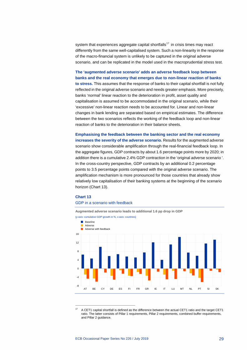
Emphasising the feedback between the banking sector and the real economy increases the severity of the adverse scenario. Results for the augmented adverse scenario show considerable amplification through the real-financial feedback loop. In the aggregate figures, GDP contracts by about 1.6 percentage points more by 2020; in addition there is a cumulative 2.4% GDP contraction in the ‘original adverse scenario ’. In the cross-country perspective, GDP contracts by an additional 0.2 percentage points to 3.5 percentage points compared with the original adverse scenario. The amplification mechanism is more pronounced for those countries that already show relatively low capitalisation of their banking systems at the beginning of the scenario horizon (Chart 13).
Chart 13 GDP in a scenario with feedback
Augmented adverse scenario leads to additional 1.6 pp drop in GDP (y-axis: cumulative GDP growth in %, x-axis: countries)
17 A CET1 capital shortfall is defined as the difference between the actual CET1 ratio and the target CET1
ratio. The latter consists of Pillar 1 requirements, Pillar 2 requirements, combined buffer requirements, and Pillar 2 guidance.
-8
-4
0
4
8
12
16
AT BE CY DE ES FI FR GR IE IT LU MT NL PT SI SK
BaselineAdverseAdverse with feedback
ECB Occasional Paper Series No 226 / July 2019
30
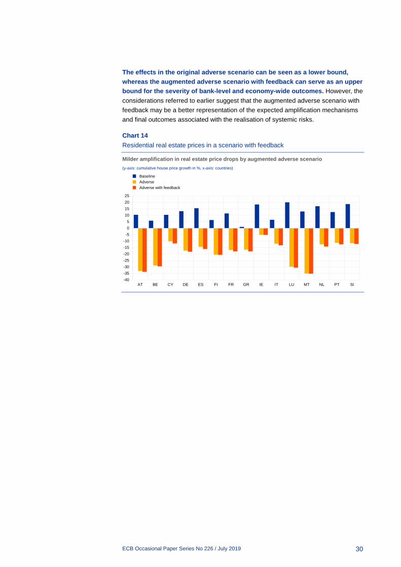
The effects in the original adverse scenario can be seen as a lower bound, whereas the augmented adverse scenario with feedback can serve as an upper bound for the severity of bank-level and economy-wide outcomes. However, the considerations referred to earlier suggest that the augmented adverse scenario with feedback may be a better representation of the expected amplification mechanisms and final outcomes associated with the realisation of systemic risks.
Chart 14 Residential real estate prices in a scenario with feedback
Milder amplification in real estate price drops by augmented adverse scenario (y-axis: cumulative house price growth in %, x-axis: countries)
-40-35-30-25-20-15-10-505
10152025
AT BE CY DE ES FI FR GR IE IT LU MT NL PT SI
BaselineAdverseAdverse with feedback
ECB Occasional Paper Series No 226 / July 2019
31
5 Discussion of selected results18
5.1 Solvency: banks deleverage to meet requirements
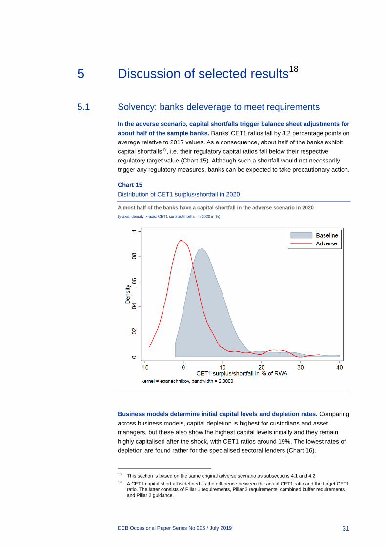
In the adverse scenario, capital shortfalls trigger balance sheet adjustments for about half of the sample banks. Banks’ CET1 ratios fall by 3.2 percentage points on average relative to 2017 values. As a consequence, about half of the banks exhibit capital shortfalls19, i.e. their regulatory capital ratios fall below their respective regulatory target value (Chart 15). Although such a shortfall would not necessarily trigger any regulatory measures, banks can be expected to take precautionary action.
Chart 15 Distribution of CET1 surplus/shortfall in 2020
Almost half of the banks have a capital shortfall in the adverse scenario in 2020 (y-axis: density, x-axis: CET1 surplus/shortfall in 2020 in %)
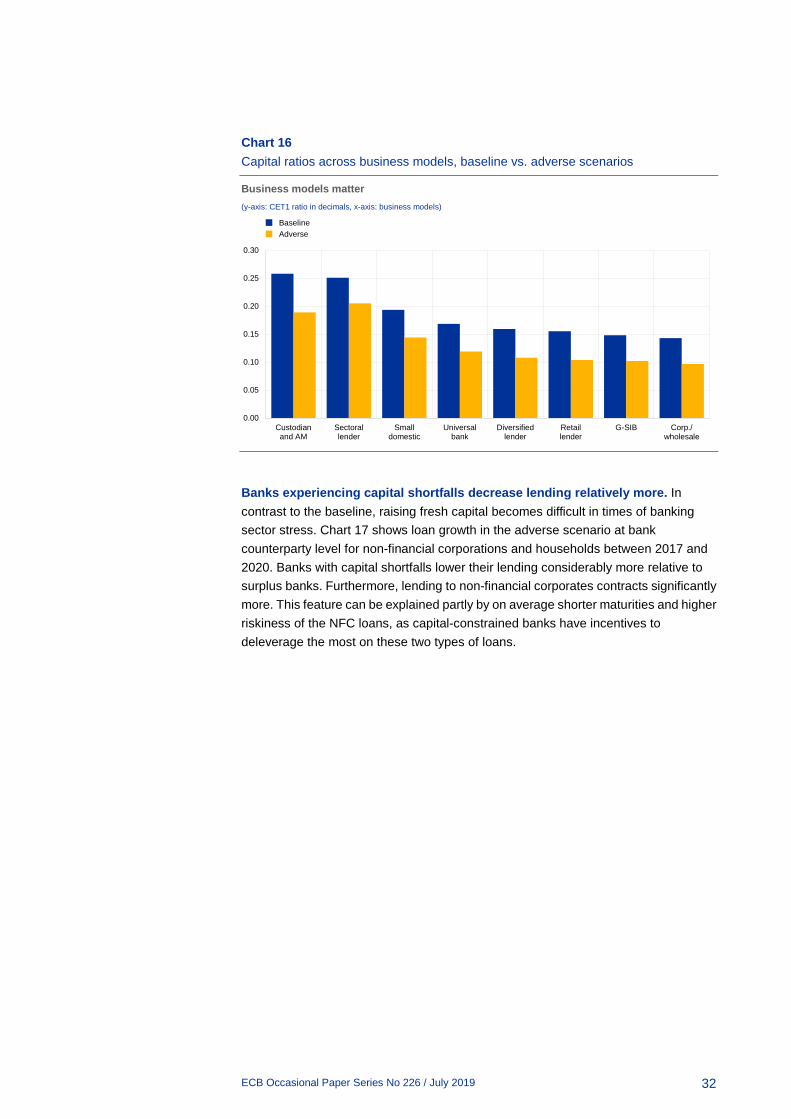
Business models determine initial capital levels and depletion rates. Comparing across business models, capital depletion is highest for custodians and asset managers, but these also show the highest capital levels initially and they remain highly capitalised after the shock, with CET1 ratios around 19%. The lowest rates of depletion are found rather for the specialised sectoral lenders (Chart 16).
18 This section is based on the same original adverse scenario as subsections 4.1 and 4.2. 19 A CET1 capital shortfall is defined as the difference between the actual CET1 ratio and the target CET1
ratio. The latter consists of Pillar 1 requirements, Pillar 2 requirements, combined buffer requirements, and Pillar 2 guidance.
ECB Occasional Paper Series No 226 / July 2019
32
Chart 16 Capital ratios across business models, baseline vs. adverse scenarios
Business models matter (y-axis: CET1 ratio in decimals, x-axis: business models)
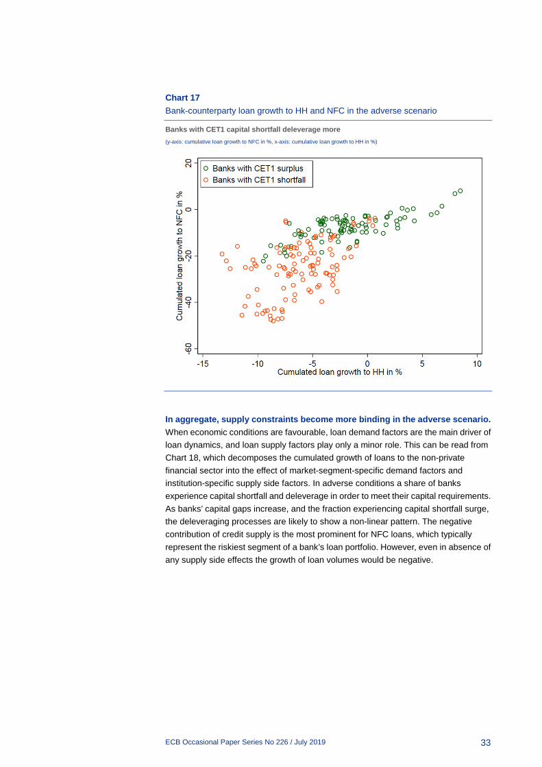
Banks experiencing capital shortfalls decrease lending relatively more. In contrast to the baseline, raising fresh capital becomes difficult in times of banking sector stress. Chart 17 shows loan growth in the adverse scenario at bank counterparty level for non-financial corporations and households between 2017 and 2020. Banks with capital shortfalls lower their lending considerably more relative to surplus banks. Furthermore, lending to non-financial corporates contracts significantly more. This feature can be explained partly by on average shorter maturities and higher riskiness of the NFC loans, as capital-constrained banks have incentives to deleverage the most on these two types of loans.
0.00
0.05
0.10
0.15
0.20
0.25
0.30
Custodianand AM
Sectorallender
Smalldomestic
Universalbank
Diversifiedlender
Retaillender
G-SIB Corp./wholesale
BaselineAdverse
ECB Occasional Paper Series No 226 / July 2019
33
Chart 17 Bank-counterparty loan growth to HH and NFC in the adverse scenario
Banks with CET1 capital shortfall deleverage more (y-axis: cumulative loan growth to NFC in %, x-axis: cumulative loan growth to HH in %)
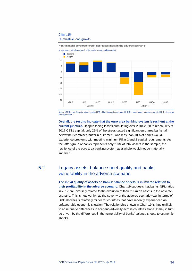
In aggregate, supply constraints become more binding in the adverse scenario. When economic conditions are favourable, loan demand factors are the main driver of loan dynamics, and loan supply factors play only a minor role. This can be read from Chart 18, which decomposes the cumulated growth of loans to the non-private financial sector into the effect of market-segment-specific demand factors and institution-specific supply side factors. In adverse conditions a share of banks experience capital shortfall and deleverage in order to meet their capital requirements. As banks’ capital gaps increase, and the fraction experiencing capital shortfall surge, the deleveraging processes are likely to show a non-linear pattern. The negative contribution of credit supply is the most prominent for NFC loans, which typically represent the riskiest segment of a bank’s loan portfolio. However, even in absence of any supply side effects the growth of loan volumes would be negative.
ECB Occasional Paper Series No 226 / July 2019
34
Chart 18 Cumulative loan growth
Non-financial corporate credit decreases most in the adverse scenario (y-axis: cumulative loan growth in %, x-axis: sectors and scenarios)
Notes: NFPS = Non-financial private sector; NFC = Non-financial corporates; HHCC = Households – consumer credit; HHHP = loans for house purchase.
Overall, the results indicate that the euro area banking system is resilient at the current juncture. Despite facing losses cumulating over 2018-2020 to reach 20% of 2017 CET1 capital, only 26% of the stress-tested significant euro area banks fall below their combined buffer requirement. And less than 10% of banks would experience problems with meeting minimum Pillar 1 and 2 capital requirements. As the latter group of banks represents only 2.8% of total assets in the sample, the resilience of the euro area banking system as a whole would not be materially impaired.
5.2 Legacy assets: balance sheet quality and banks’ vulnerability in the adverse scenario
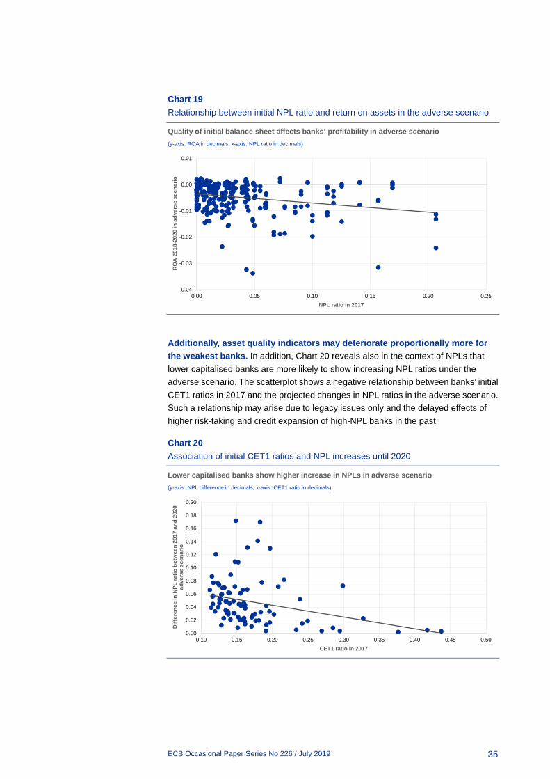
The initial quality of assets on banks’ balance sheets is in inverse relation to their profitability in the adverse scenario. Chart 19 suggests that banks’ NPL ratios in 2017 are inversely related to the evolution of their return on assets in the adverse scenario. This is noteworthy, as the severity of the adverse scenario (e.g. in terms of GDP decline) is relatively milder for countries that have recently experienced an unfavourable economic situation. The relationship shown in Chart 19 is thus unlikely to arise due to differences in scenario adversity across countries alone. It may in turn be driven by the differences in the vulnerability of banks’ balance sheets to economic shocks.
-25
-20
-15
-10
-5
0
5
10
NFPS NFC HHCC HHHP NFPS NFC HHCC HHHP
Baseline Adverse
DemandSupply
ECB Occasional Paper Series No 226 / July 2019
35
Chart 19 Relationship between initial NPL ratio and return on assets in the adverse scenario
Quality of initial balance sheet affects banks’ profitability in adverse scenario (y-axis: ROA in decimals, x-axis: NPL ratio in decimals)
Additionally, asset quality indicators may deteriorate proportionally more for the weakest banks. In addition, Chart 20 reveals also in the context of NPLs that lower capitalised banks are more likely to show increasing NPL ratios under the adverse scenario. The scatterplot shows a negative relationship between banks’ initial CET1 ratios in 2017 and the projected changes in NPL ratios in the adverse scenario. Such a relationship may arise due to legacy issues only and the delayed effects of higher risk-taking and credit expansion of high-NPL banks in the past.
Chart 20 Association of initial CET1 ratios and NPL increases until 2020
Lower capitalised banks show higher increase in NPLs in adverse scenario (y-axis: NPL difference in decimals, x-axis: CET1 ratio in decimals)
-0.04
-0.03
-0.02
-0.01
0.00
0.01
0.00 0.05 0.10 0.15 0.20 0.25
RO
A 2
018-
2020
in a
dver
se s
cena
rio
NPL ratio in 2017
0.00
0.02
0.04
0.06
0.08
0.10
0.12
0.14
0.16
0.18
0.20
0.10 0.15 0.20 0.25 0.30 0.35 0.40 0.45 0.50
Diff
eren
ce in
NPL
ratio
bet
wee
n 20
17 a
nd 2
020
adve
rse
scen
ario
CET1 ratio in 2017
ECB Occasional Paper Series No 226 / July 2019
36
5.3 Vulnerabilities: low profitability and low capital
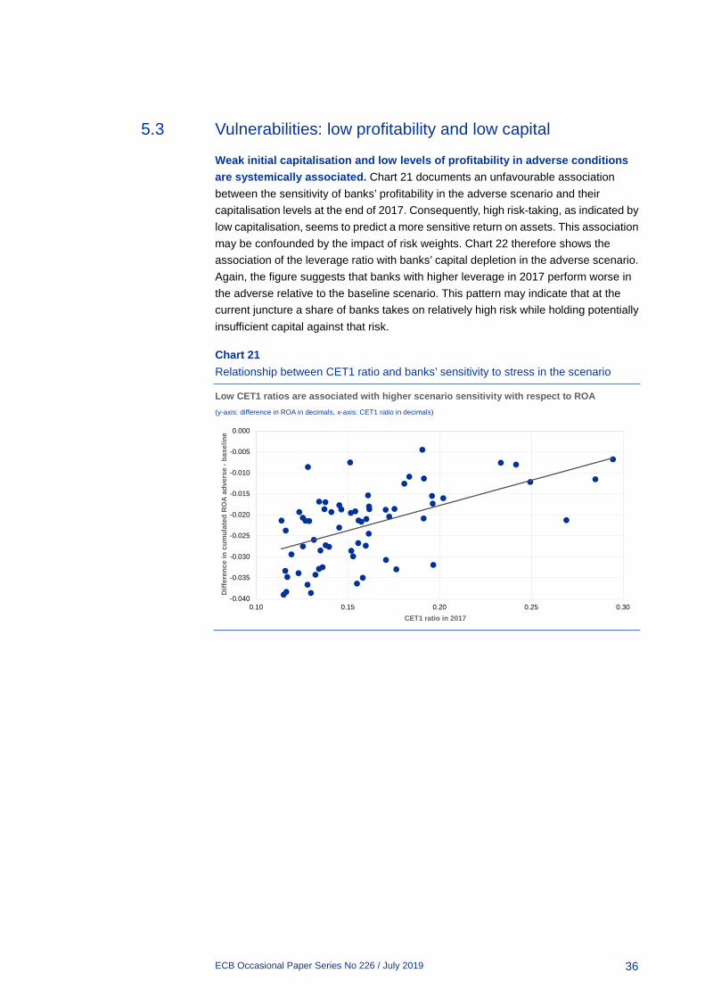
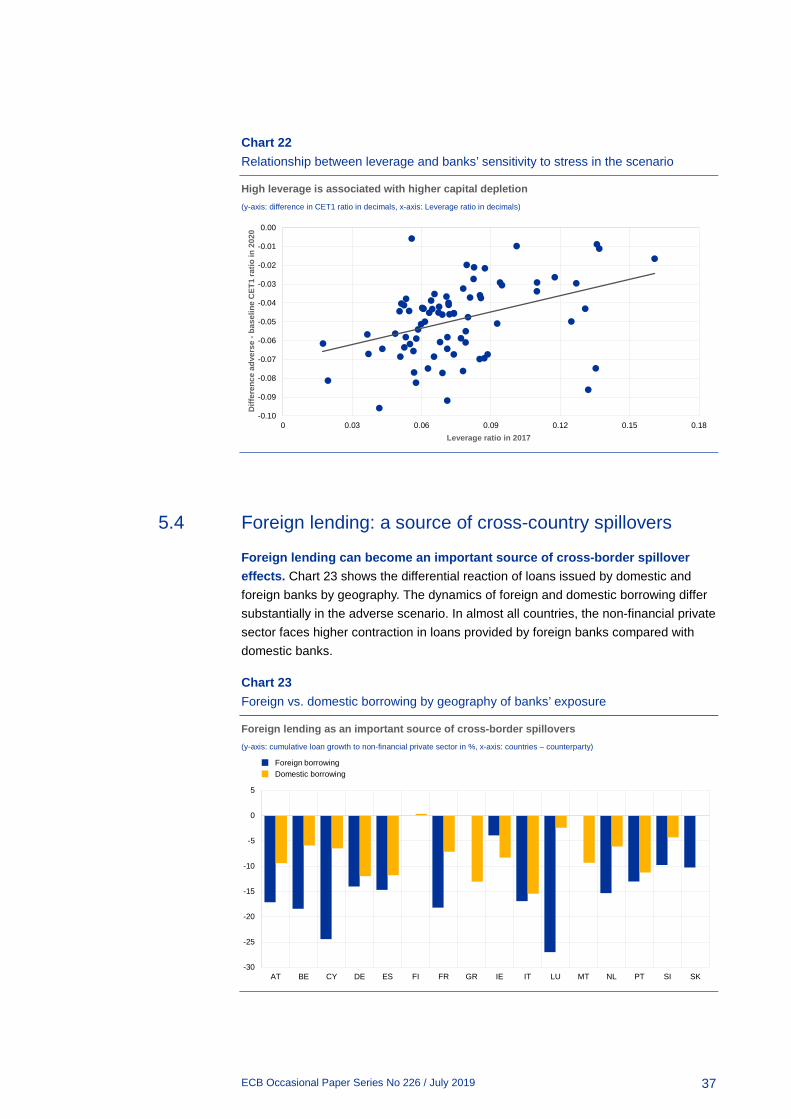
Weak initial capitalisation and low levels of profitability in adverse conditions are systemically associated. Chart 21 documents an unfavourable association between the sensitivity of banks’ profitability in the adverse scenario and their capitalisation levels at the end of 2017. Consequently, high risk-taking, as indicated by low capitalisation, seems to predict a more sensitive return on assets. This association may be confounded by the impact of risk weights. Chart 22 therefore shows the association of the leverage ratio with banks’ capital depletion in the adverse scenario. Again, the figure suggests that banks with higher leverage in 2017 perform worse in the adverse relative to the baseline scenario. This pattern may indicate that at the current juncture a share of banks takes on relatively high risk while holding potentially insufficient capital against that risk.
Chart 21 Relationship between CET1 ratio and banks’ sensitivity to stress in the scenario
Low CET1 ratios are associated with higher scenario sensitivity with respect to ROA (y-axis: difference in ROA in decimals, x-axis: CET1 ratio in decimals)
-0.040
-0.035
-0.030
-0.025
-0.020
-0.015
-0.010
-0.005
0.000
0.10 0.15 0.20 0.25 0.30
Diff
eren
ce in
cum
ulat
ed R
OA
adv
erse
-ba
selin
e
CET1 ratio in 2017
ECB Occasional Paper Series No 226 / July 2019
37
Chart 22 Relationship between leverage and banks’ sensitivity to stress in the scenario
High leverage is associated with higher capital depletion (y-axis: difference in CET1 ratio in decimals, x-axis: Leverage ratio in decimals)
5.4 Foreign lending: a source of cross-country spillovers
Foreign lending can become an important source of cross-border spillover effects. Chart 23 shows the differential reaction of loans issued by domestic and foreign banks by geography. The dynamics of foreign and domestic borrowing differ substantially in the adverse scenario. In almost all countries, the non-financial private sector faces higher contraction in loans provided by foreign banks compared with domestic banks.
Chart 23 Foreign vs. domestic borrowing by geography of banks’ exposure
Foreign lending as an important source of cross-border spillovers (y-axis: cumulative loan growth to non-financial private sector in %, x-axis: countries – counterparty)
-0.10
-0.09
-0.08
-0.07
-0.06
-0.05
-0.04
-0.03
-0.02
-0.01
0.00
0 0.03 0.06 0.09 0.12 0.15 0.18
Diff
eren
ce a
dver
se -
base
line
CET
1 ra
tio in
202
0
Leverage ratio in 2017
-30
-25
-20
-15
-10
-5
0
5
AT BE CY DE ES FI FR GR IE IT LU MT NL PT SI SK
Foreign borrowingDomestic borrowing
ECB Occasional Paper Series No 226 / July 2019
38
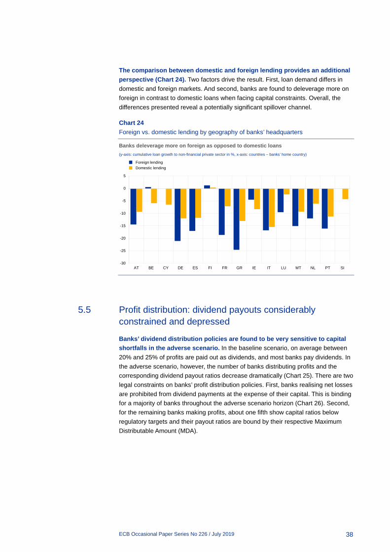
The comparison between domestic and foreign lending provides an additional perspective (Chart 24). Two factors drive the result. First, loan demand differs in domestic and foreign markets. And second, banks are found to deleverage more on foreign in contrast to domestic loans when facing capital constraints. Overall, the differences presented reveal a potentially significant spillover channel.
Chart 24 Foreign vs. domestic lending by geography of banks’ headquarters
Banks deleverage more on foreign as opposed to domestic loans (y-axis: cumulative loan growth to non-financial private sector in %, x-axis: countries – banks’ home country)
5.5 Profit distribution: dividend payouts considerably constrained and depressed
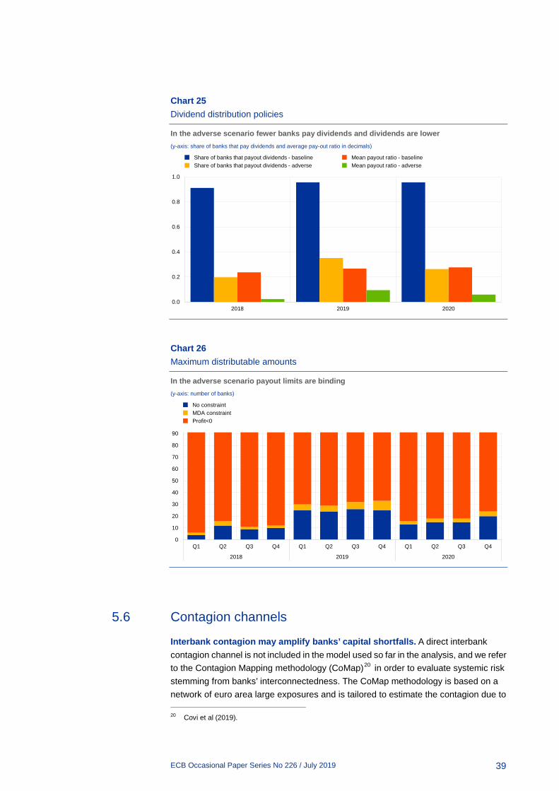
Banks’ dividend distribution policies are found to be very sensitive to capital shortfalls in the adverse scenario. In the baseline scenario, on average between 20% and 25% of profits are paid out as dividends, and most banks pay dividends. In the adverse scenario, however, the number of banks distributing profits and the corresponding dividend payout ratios decrease dramatically (Chart 25). There are two legal constraints on banks’ profit distribution policies. First, banks realising net losses are prohibited from dividend payments at the expense of their capital. This is binding for a majority of banks throughout the adverse scenario horizon (Chart 26). Second, for the remaining banks making profits, about one fifth show capital ratios below regulatory targets and their payout ratios are bound by their respective Maximum Distributable Amount (MDA).
-30
-25
-20
-15
-10
-5
0
5
AT BE CY DE ES FI FR GR IE IT LU MT NL PT SI
Foreign lendingDomestic lending
ECB Occasional Paper Series No 226 / July 2019
39
Chart 25 Dividend distribution policies
In the adverse scenario fewer banks pay dividends and dividends are lower (y-axis: share of banks that pay dividends and average pay-out ratio in decimals)
Chart 26 Maximum distributable amounts
In the adverse scenario payout limits are binding (y-axis: number of banks)
5.6 Contagion channels
Interbank contagion may amplify banks’ capital shortfalls. A direct interbank contagion channel is not included in the model used so far in the analysis, and we refer to the Contagion Mapping methodology (CoMap)20 in order to evaluate systemic risk stemming from banks’ interconnectedness. The CoMap methodology is based on a network of euro area large exposures and is tailored to estimate the contagion due to 20 Covi et al (2019).
0.0
0.2
0.4
0.6
0.8
1.0
2018 2019 2020
Share of banks that payout dividends - baselineShare of banks that payout dividends - adverse
Mean payout ratio - baselineMean payout ratio - adverse
0
10
20
30
40
50
60
70
80
90
Q1 Q2 Q3 Q4 Q1 Q2 Q3 Q4 Q1 Q2 Q3 Q4
2018 2019 2020
No constraintMDA constraintProfit<0
ECB Occasional Paper Series No 226 / July 2019
40
credit and funding risks via bilateral linkages. It evaluates first-round effects (direct losses), and second-round (and subsequent) effects (cascade losses) due to domino defaults and fire sale losses as banks respond to shocks by liquidating assets.
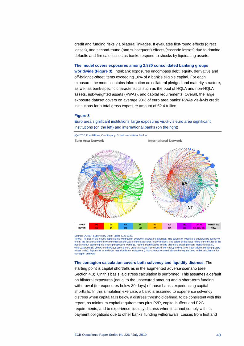
The model covers exposures among 2,830 consolidated banking groups worldwide (Figure 3). Interbank exposures encompass debt, equity, derivative and off-balance-sheet items exceeding 10% of a bank’s eligible capital. For each exposure, the model contains information on collateral pledged and maturity structure, as well as bank-specific characteristics such as the pool of HQLA and non-HQLA assets, risk-weighted assets (RWAs), and capital requirements. Overall, the large exposure dataset covers on average 90% of euro area banks’ RWAs vis-à-vis credit institutions for a total gross exposure amount of €2.4 trillion.
Figure 3 Euro area significant institutions’ large exposures vis-à-vis euro area significant institutions (on the left) and international banks (on the right)
(Q4-2017; Euro Billions, Counterparty: SI and International Banks)
Euro Area Network International Network
Source: COREP Supervisory Data: Tables C.27-C.28. Notes: The size of the nodes captures the weighted in-degree of interconnectedness. The colours of nodes are clustered by country of origin, the thickness of the flows summarises the value of the exposures in EUR billions. The colour of the flows refers to the source of the node’s colour capturing the lender perspective. Panel (a) reports interlinkages among only euro area significant institutions (Sis), whereas panel (b) shows interlinkages among euro area significant institutions (inner circle) and vis-à-vis international banking groups (outer circle). Exposures to and from less significant institutions (LSIs) are not reported, although they are used in the calculations for contagion analysis.
The contagion calculation covers both solvency and liquidity distress. The starting point is capital shortfalls as in the augmented adverse scenario (see Section 4.3). On this basis, a distress calculation is performed. This assumes a default on bilateral exposures (equal to the unsecured amount) and a short-term funding withdrawal (for exposures below 30 days) of those banks experiencing capital shortfalls. In this simulation exercise, a bank is assumed to experience solvency distress when capital falls below a distress threshold defined, to be consistent with this report, as minimum capital requirements plus P2R, capital buffers and P2G requirements, and to experience liquidity distress when it cannot comply with its payment obligations due to other banks’ funding withdrawals. Losses from first and
EA
INT
INNER DE ES FR IT NL AT BE LU, FI OTHER EAOUTER CN JP US UK TR CA CH SE, NO, DK ROW
ECB Occasional Paper Series No 226 / July 2019
41
subsequent rounds are accrued to the initial capital shortfalls. The contagion is computed as one-off effects for each quarter in the three-year stress-test horizon and it does not feed back to the rest of the economy.
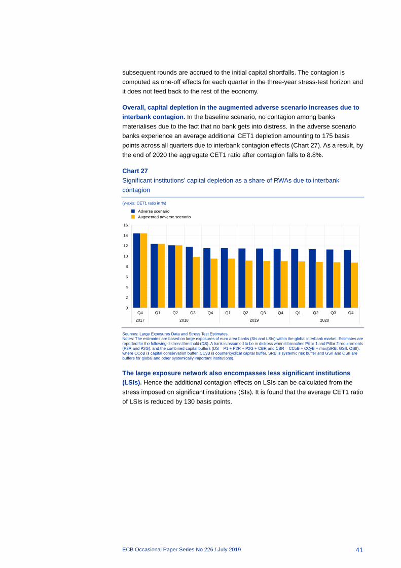
Overall, capital depletion in the augmented adverse scenario increases due to interbank contagion. In the baseline scenario, no contagion among banks materialises due to the fact that no bank gets into distress. In the adverse scenario banks experience an average additional CET1 depletion amounting to 175 basis points across all quarters due to interbank contagion effects (Chart 27). As a result, by the end of 2020 the aggregate CET1 ratio after contagion falls to 8.8%.
Chart 27 Significant institutions’ capital depletion as a share of RWAs due to interbank contagion
(y-axis: CET1 ratio in %)
Sources: Large Exposures Data and Stress Test Estimates. Notes: The estimates are based on large exposures of euro area banks (SIs and LSIs) within the global interbank market. Estimates are reported for the following distress threshold (DS). A bank is assumed to be in distress when it breaches Pillar 1 and Pillar 2 requirements (P2R and P2G), and the combined capital buffers (DS = P1 + P2R + P2G + CBR and CBR = CCoB + CCyB + max(SRB, GSII, OSII), where CCoB is capital conservation buffer, CCyB is countercyclical capital buffer, SRB is systemic risk buffer and GSII and OSII are buffers for global and other systemically important institutions).
The large exposure network also encompasses less significant institutions (LSIs). Hence the additional contagion effects on LSIs can be calculated from the stress imposed on significant institutions (SIs). It is found that the average CET1 ratio of LSIs is reduced by 130 basis points.
0
2
4
6
8
10
12
14
16
Q4 Q1 Q2 Q3 Q4 Q1 Q2 Q3 Q4 Q1 Q2 Q3 Q4
2017 2018 2019 2020
Adverse scenarioAugmented adverse scenario
ECB Occasional Paper Series No 226 / July 2019
42
6 The role of non-bank financial intermediaries
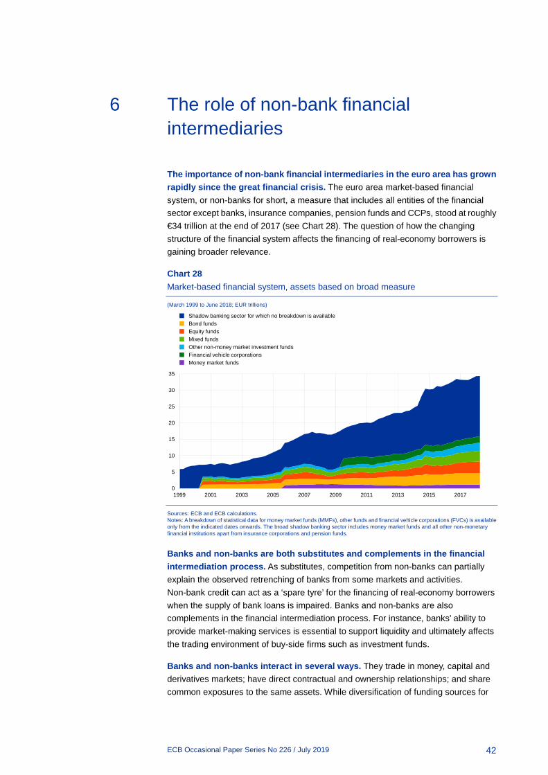
The importance of non-bank financial intermediaries in the euro area has grown rapidly since the great financial crisis. The euro area market-based financial system, or non-banks for short, a measure that includes all entities of the financial sector except banks, insurance companies, pension funds and CCPs, stood at roughly €34 trillion at the end of 2017 (see Chart 28). The question of how the changing structure of the financial system affects the financing of real-economy borrowers is gaining broader relevance.
Chart 28 Market-based financial system, assets based on broad measure
(March 1999 to June 2018; EUR trillions)
Sources: ECB and ECB calculations. Notes: A breakdown of statistical data for money market funds (MMFs), other funds and financial vehicle corporations (FVCs) is available only from the indicated dates onwards. The broad shadow banking sector includes money market funds and all other non-monetary financial institutions apart from insurance corporations and pension funds.
Banks and non-banks are both substitutes and complements in the financial intermediation process. As substitutes, competition from non-banks can partially explain the observed retrenching of banks from some markets and activities. Non-bank credit can act as a ‘spare tyre’ for the financing of real-economy borrowers when the supply of bank loans is impaired. Banks and non-banks are also complements in the financial intermediation process. For instance, banks’ ability to provide market-making services is essential to support liquidity and ultimately affects the trading environment of buy-side firms such as investment funds.
Banks and non-banks interact in several ways. They trade in money, capital and derivatives markets; have direct contractual and ownership relationships; and share common exposures to the same assets. While diversification of funding sources for
0
5
10
15
20
25
30
35
1999 2001 2003 2005 2007 2009 2011 2013 2015 2017
Shadow banking sector for which no breakdown is availableBond fundsEquity fundsMixed fundsOther non-money market investment fundsFinancial vehicle corporationsMoney market funds
ECB Occasional Paper Series No 226 / July 2019
43
real-economy borrowers normally contributes to the efficiency of financial intermediation, some types of interaction between banks and non-banks can contribute to amplifying shocks. Contagion channels and spillovers include the materialisation of credit and counterparty risk from direct exposures, risks associated with liquidity and maturity transformation of open-end investment funds, price-mediated mechanisms due to overlapping portfolios, and contingent liabilities from derivatives contracts.
This section proposes three exercises that delve deeper into the possible behaviour of non-banks in the adverse scenario envisaged by the stress test. The discussion around system-wide stress analysis, i.e. the idea of modelling the complex interactions between banks and non-banks in a unified, consistent framework, is still open. In turn, this section presents three exercises, each of them providing one specific angle on the behaviour of non-banks in the scenario. The first exercise helps to understand how the scenario could directly impact inflows and outflows for different types of investment fund, the fast-growing entities in the non-bank universe. The second exercise investigates how banks and investment funds could interact in an environment of asset fire sales. Finally, the third exercise discusses how and to what extent non-bank finance could substitute for a decline in bank loans to non-financial corporations.
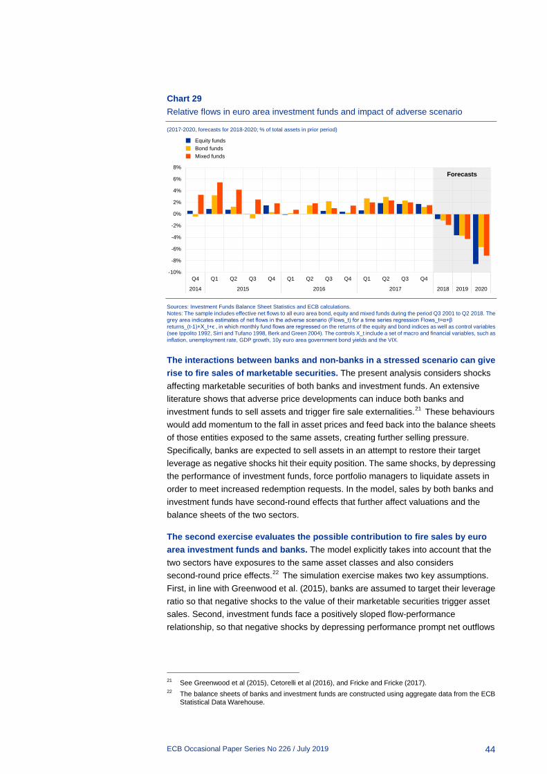
Equity, bond and mixed investment funds are expected to experience large outflows in the adverse scenario (Chart 29). The first exercise focuses on expected flows in and out of euro area investment funds under the adverse scenario. Since the crisis, the euro area asset management complex has experienced continued and strong growth, mirroring a global trend. Total assets of euro area investment funds were roughly €12 trillion in March 2018, almost three times their level back in 2008. In this very simple exercise, effective net flows experienced by different categories of investment funds during the period Q3 2001 to Q2 2018 are regressed on a set of macro and financial market variables. These results are then used to estimate net inflows, given the macro and financial conditions envisaged under the adverse scenario in the period 2018-20. Estimated outflows are significant for all funds, with equity funds expected to experience major falls in assets under management due to large losses for equity indices envisaged in the adverse scenario.
ECB Occasional Paper Series No 226 / July 2019
44
Chart 29 Relative flows in euro area investment funds and impact of adverse scenario
(2017-2020, forecasts for 2018-2020; % of total assets in prior period)
Sources: Investment Funds Balance Sheet Statistics and ECB calculations. Notes: The sample includes effective net flows to all euro area bond, equity and mixed funds during the period Q3 2001 to Q2 2018. The grey area indicates estimates of net flows in the adverse scenario (Flows_t) for a time series regression Flows_t=α+β returns_(t-1)+X_t+ϵ , in which monthly fund flows are regressed on the returns of the equity and bond indices as well as control variables (see Ippolito 1992, Sirri and Tufano 1998, Berk and Green 2004). The controls X_t include a set of macro and financial variables, such as inflation, unemployment rate, GDP growth, 10y euro area government bond yields and the VIX.
The interactions between banks and non-banks in a stressed scenario can give rise to fire sales of marketable securities. The present analysis considers shocks affecting marketable securities of both banks and investment funds. An extensive literature shows that adverse price developments can induce both banks and investment funds to sell assets and trigger fire sale externalities.21 These behaviours would add momentum to the fall in asset prices and feed back into the balance sheets of those entities exposed to the same assets, creating further selling pressure. Specifically, banks are expected to sell assets in an attempt to restore their target leverage as negative shocks hit their equity position. The same shocks, by depressing the performance of investment funds, force portfolio managers to liquidate assets in order to meet increased redemption requests. In the model, sales by both banks and investment funds have second-round effects that further affect valuations and the balance sheets of the two sectors.
The second exercise evaluates the possible contribution to fire sales by euro area investment funds and banks. The model explicitly takes into account that the two sectors have exposures to the same asset classes and also considers second-round price effects.22 The simulation exercise makes two key assumptions. First, in line with Greenwood et al. (2015), banks are assumed to target their leverage ratio so that negative shocks to the value of their marketable securities trigger asset sales. Second, investment funds face a positively sloped flow-performance relationship, so that negative shocks by depressing performance prompt net outflows
21 See Greenwood et al (2015), Cetorelli et al (2016), and Fricke and Fricke (2017). 22 The balance sheets of banks and investment funds are constructed using aggregate data from the ECB
Statistical Data Warehouse.
-10%
-8%
-6%
-4%
-2%
0%
2%
4%
6%
8%
Q4 Q1 Q2 Q3 Q4 Q1 Q2 Q3 Q4 Q1 Q2 Q3 Q4
2014 2015 2016 2017 2018 2019 2020
Equity fundsBond fundsMixed funds
Forecasts
ECB Occasional Paper Series No 226 / July 2019
45
and, ultimately, asset sales to accommodate redemption requests.23 The impact of asset sales on prices is calculated using the Amihud ratio of relevant market indices for equity holdings and, for debt securities.24
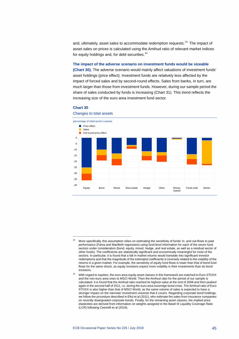
The impact of the adverse scenario on investment funds would be sizeable (Chart 30). The adverse scenario would mainly affect valuations of investment funds’ asset holdings (price effect). Investment funds are relatively less affected by the impact of forced sales and by second-round effects. Sales from banks, in turn, are much larger than those from investment funds. However, during our sample period the share of sales conducted by funds is increasing (Chart 31). This trend reflects the increasing size of the euro area investment fund sector.
Chart 30 Changes to total assets
(percentage of initial sector’s assets)
23 More specifically, this assumption relies on estimating the sensitivity of funds’ in- and out-flows to past
performance (Fama and MacBeth regression) using fund-level information for each of the seven fund sectors under consideration (bond, equity, mixed, hedge, and real estate, as well as a residual sector of other funds). The coefficients are statistically significant and economically meaningful for most of the sectors. In particular, it is found that a fall in market returns would translate into significant investor redemptions and that the magnitude of the estimated coefficients is inversely related to the volatility of the returns in a given market. For example, the sensitivity of equity fund flows is lower than that of bond fund flows for the same shock, as equity investors expect more volatility in their investments than do bond investors.
24 With regard to equities, the euro area equity asset classes in this framework are matched to Euro STOXX and the non-euro area ones to MSCI World. Then the Amihud ratio for the period of our sample is calculated. It is found that the Amihud ratio reached its highest value at the end of 2008 and then peaked again in the second half of 2011, i.e. during the euro area sovereign bond crisis. The Amihud ratio of Euro STOXX is also higher than that of MSCI World, as the same volume of sales is expected to have a stronger impact on the narrower investment universe that it covers. Regarding corporate bond holdings, we follow the procedure described in Ellul et al (2011), who estimate fire sales from insurance companies on recently downgraded corporate bonds. Finally, for the remaining asset classes, the implied price elasticities are derived from information on weights assigned in the Basel III Liquidity Coverage Ratio (LCR) following Cetorelli et al (2016).
-40
-35
-30
-25
-20
-15
-10
-5
0
Equity Bond Mixed Real estate Hedge Other Moneymarket
Funds total Banks
Price effectSales2nd round price effect
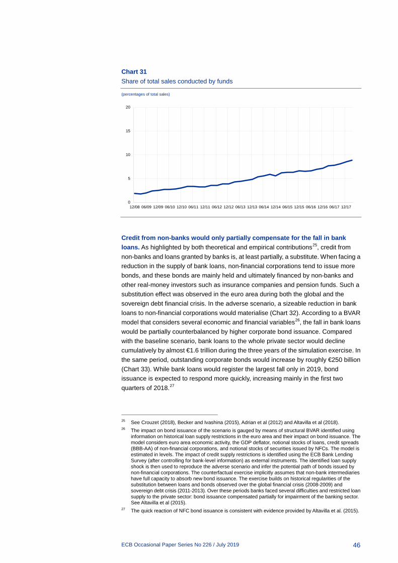
ECB Occasional Paper Series No 226 / July 2019
46
Chart 31 Share of total sales conducted by funds
(percentages of total sales)
Credit from non-banks would only partially compensate for the fall in bank loans. As highlighted by both theoretical and empirical contributions25, credit from non-banks and loans granted by banks is, at least partially, a substitute. When facing a reduction in the supply of bank loans, non-financial corporations tend to issue more bonds, and these bonds are mainly held and ultimately financed by non-banks and other real-money investors such as insurance companies and pension funds. Such a substitution effect was observed in the euro area during both the global and the sovereign debt financial crisis. In the adverse scenario, a sizeable reduction in bank loans to non-financial corporations would materialise (Chart 32). According to a BVAR model that considers several economic and financial variables26, the fall in bank loans would be partially counterbalanced by higher corporate bond issuance. Compared with the baseline scenario, bank loans to the whole private sector would decline cumulatively by almost €1.6 trillion during the three years of the simulation exercise. In the same period, outstanding corporate bonds would increase by roughly €250 billion (Chart 33). While bank loans would register the largest fall only in 2019, bond issuance is expected to respond more quickly, increasing mainly in the first two quarters of 2018.27
25 See Crouzet (2018), Becker and Ivashina (2015), Adrian et al (2012) and Altavilla et al (2018). 26 The impact on bond issuance of the scenario is gauged by means of structural BVAR identified using
information on historical loan supply restrictions in the euro area and their impact on bond issuance. The model considers euro area economic activity, the GDP deflator, notional stocks of loans, credit spreads (BBB-AA) of non-financial corporations, and notional stocks of securities issued by NFCs. The model is estimated in levels. The impact of credit supply restrictions is identified using the ECB Bank Lending Survey (after controlling for bank-level information) as external instruments. The identified loan supply shock is then used to reproduce the adverse scenario and infer the potential path of bonds issued by non-financial corporations. The counterfactual exercise implicitly assumes that non-bank intermediaries have full capacity to absorb new bond issuance. The exercise builds on historical regularities of the substitution between loans and bonds observed over the global financial crisis (2008-2009) and sovereign debt crisis (2011-2013). Over these periods banks faced several difficulties and restricted loan supply to the private sector: bond issuance compensated partially for impairment of the banking sector. See Altavilla et al (2015).
27 The quick reaction of NFC bond issuance is consistent with evidence provided by Altavilla et al. (2015).
0
5
10
15
20
12/08 06/09 12/09 06/10 12/10 06/11 12/11 06/12 12/12 06/13 12/13 06/14 12/14 06/15 12/15 06/16 12/16 06/17 12/17
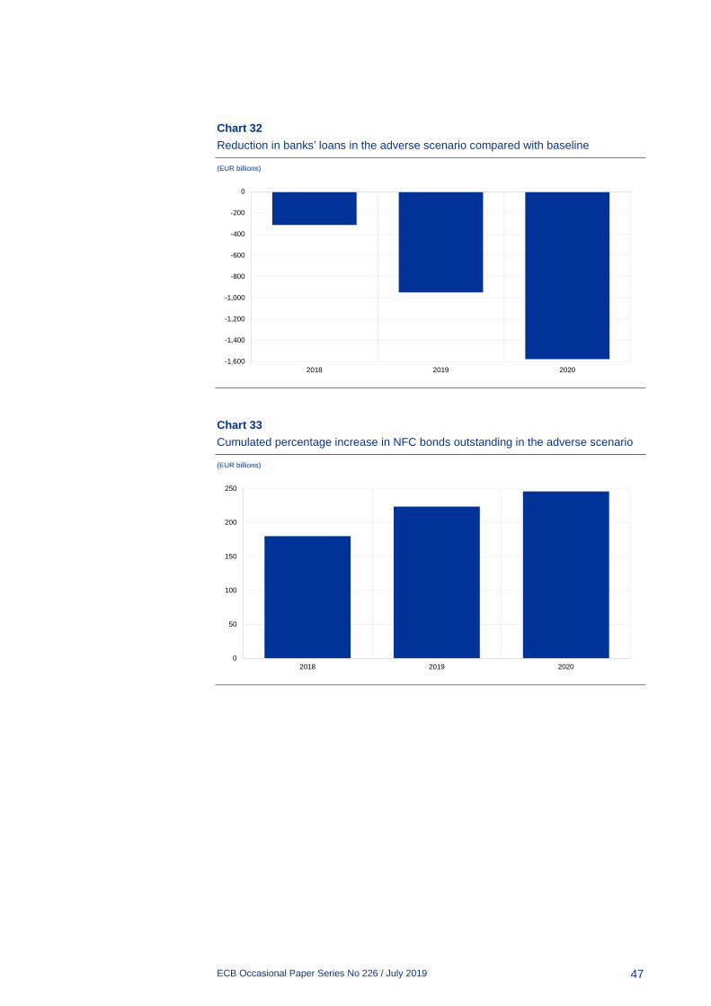
ECB Occasional Paper Series No 226 / July 2019
47
Chart 32 Reduction in banks’ loans in the adverse scenario compared with baseline
(EUR billions)
Chart 33 Cumulated percentage increase in NFC bonds outstanding in the adverse scenario
(EUR billions)
-1,600
-1,400
-1,200
-1,000
-800
-600
-400
-200
0
2018 2019 2020
0
50
100
150
200
250
2018 2019 2020
ECB Occasional Paper Series No 226 / July 2019
48
7 Conclusions
In this paper we present a macroprudential stress test for 91 significant euro area banks. The stress test considers the evolution of the financial system as a whole and includes various amplification mechanisms. It starts from an adverse but plausible macroeconomic scenario, and includes banks’ endogenous responses to shocks. By including bank reactions, it offers a metric for judging the resilience of the banking sector that incorporates banks’ behaviour according to historically observed patterns. The paper also evaluates the effect of adding the feedback loops between the financial and real sectors, as well as the interactions between banks and other counterparties in financial and capital markets.
The stress test exercise illustrates the relevance of assumptions regarding banks’ behaviour, especially of a static vs. a dynamic balance sheet assumption. Compared with the results under the static balance sheet assumption, which is typically applied in the microprudential stress test exercise, under the dynamic balance sheet assumption this paper finds lower depletion in terms of the CET1 ratio, but higher depletion in terms of absolute system-wide CET1 capital. The lower depletion of capital ratios results from banks’ deleveraging that improves their capital ratios compared with the results under the static balance sheet assumption. In contrast, the higher depletion in terms of absolute system-wide capital is driven by the additional amplification mechanisms that increase losses and hence lower capital, though banks still deleverage and mute the effect on their capital ratios. The deleveraging, however, constitutes an externality and imposes costs in terms of an additional credit contraction that translates into lower economic activity. For the adverse scenario considered, a credit supply shock propagates back to the real economy and results in an additional 1.6 percentage point decrease in euro area cumulative GDP growth.
The proposed methodology for the macroprudential stress test will develop further. The results presented are based on many exogenous paths of bank-level variables that are intended to be endogenised in future versions of the model. This concerns for instance the market risk or selected components of funding costs. Further, semi-structural approach, while overcoming many modelling obstacles, is still not free from limitations imposed by generally low bank-level and loan-level data availability. For instance, separate estimation of many model equations may foster higher estimation errors. To address the latter concern at least partially, one of the appendices of the paper reports the results of an outside model validation of the reported results.
ECB Occasional Paper Series No 226 / July 2019
49
References
Adrian, T., Colla, P. and Shin, H. (2013), “Which Financial Frictions? Parsing the Evidence from the Financial Crisis of 2007 to 2009”, NBER Macroeconomics Annual, 27, issue 1, p. 159 – 214.
Altavilla, C., Darracq Pariès, M. and Nicoletti, G. (2015), “Loan supply, credit markets and the euro area financial crisis”, Working Paper Series, No 1861, European Central Bank.
Barnett, A. and Thomas, R. (2013), “Has weak lending and activity in the United Kingdom been driven by credit supply shocks?” Bank of England working papers, No 482, Bank of England.
Becker, B. and Ivashina, V. (2015), “Reaching for Yield in the Bond Market”, Journal of Finance, 70, issue 5, p. 1863-1902.
Brinkhoff, J., Langfield, S. and Weeken, O. (2018), “From the horse’s mouth: surveying responses to stress by banks and insurers”, ESRB Occasional Paper Series No 15 / April 2018
Budnik, K., Balatti, M, Dimitrov, I., Gross, J, Kleemann, M., Reichenbachas, T., Sanna, F., Sarychev, A., Sinienko, N. and Volk, M. (2019), “Banking euro area stress test model”, manuscript to be published in Autumn 2019
Covi, G., Gorpe, M.Z. and Kok, C. (2019), “CoMap: Mapping Contagion in the Euro Area Banking Sector”, ECB Working Paper, No 2224.
Cetorelli, N., Duarte, F. and Eisenbach T. (2016), "Are Asset Managers Vulnerable to Fire Sales?”. Blogpost Liberty Street Economics (Feb 18, 2016)
Crouzet, N. (2018), “Aggregate Implications of Corporate Debt Choices," Review of Economic Studies, Oxford University Press, vol. 85(3), pages 1635-1682.
Cummings, J.R. and Durrani, K.J. (2016), “Regulatory capital and internal capital targets: An examination of the Australian banking industry”, CIFR Paper No 112/2016 / Project T023.
Dees, S., Henry, J., and Martin, R. (2017), “STAMP€: Stress-test analytics for macroprudential purposes in the euro area”, European Central Bank.
Duchi, F. and Elbourne, A. (2016), “Credit supply shocks in the Netherlands”, Journal of Macroeconomics, Vol. 50(C), Elsevier, pp. 51-71.
Ellul, A., Chotibhak, J., and Lundblad, Ch. (2011), "Regulatory pressure and fire sales in the corporate bond market." Journal of Financial Economics 101.3, pp. 596-620.
ECB Occasional Paper Series No 226 / July 2019
50
Espinosa-Vega, M. and Solé, J. (2011), "Cross-border financial surveillance: a network perspective," Journal of Financial Economic Policy, Emerald Group Publishing, vol. 3(3), pp. 182-205.
Greetje Everaert, G., Che, N., Geng, N., Gruss, B., Impavido, G., Lu, Y., Saborowski, Ch., Vandenbussche, J., and Zeng, L. (2015), ” Supply or Demand Drive the Credit Cycle? Evidence from Central, Eastern, and Southeastern Europe”, IMF Working Papers 15/15.
Estrella, A. (2004), “The cyclical behavior of optimal bank capital”, Journal of Banking and Finance, Vol. 28, No 6, pp. 1469-1498.
ESRB (2018), “Adverse macro-financial scenario for the 2018 EU-wide banking sector stress test”.
Fricke, Ch. and Fricke, D. (2017), “Vulnerable Asset Management? The Case of Mutual Funds”, Bundesbank Discussion Paper No. 32/2017
Greenwood, R., Landier, A. and Thesmar, D. (2015), “Vulnerable banks”, Journal of Financial Economics, 115, issue 3, p. 471-485.
Hristov, N., Hülsewig, O. and Wollmershäuser, T. (2012), "Loan supply shocks during the financial crisis: Evidence for the Euro area," Journal of International Money and Finance, Elsevier, vol. 31(3), pages 569-592.
IMF (2018). IMF Country Report No. 18/226
Khwaja A.I. and Mian A. (2008). Tracing the impact of bank liquidity shocks: Evidence from an emerging market. The American Economic Review, 98(4):1413–1442.
ECB Occasional Paper Series No 226 / July 2019
51
Appendices
Appendix 1: Implementation of the feedback loop and cure rates
Model and feedback loop
This appendix elaborates on the design of the feedback loop in the augmented adverse scenario. The details of the model and its dynamics are described in the accompanying paper “Banking euro area stress test model” (BEAST), while the appendix summarises only the functioning of selected elements of the model relevant to implementation of the feedback loop.
The macroeconomic module of the BEAST can be described as a reduced-form multi-country setup. The dynamics of single euro area economies are estimated using a structural panel vector autoregressive model (SPVAR). An additional block of cross-country trade spillovers links countries’ import volumes to foreign demand variables, and their export prices to foreign price variables.
The SPVAR distinguishes between 10 structural shocks. It is estimated for 19 euro area countries and includes 11 endogenous and two exogenous variables for each country. Credit supply shock in particular is identified by a set of sign and zero restrictions following Hristov et al. (2012), Barnett et al. (2013) and Duchi et al. (2016). It leads to lending rates and lending volumes moving in opposite directions. To distinguish the shock from aggregated demand innovations we also impose zero contemporaneous restrictions on price inflation, unemployment rate, and short- and long-term interest rates. Along with the estimates, on average a favourable credit supply shock increases loan volume by about 1.1% on impact and decreases lending rates by 5 basis points on impact. After the credit supply shock, GDP increases by about 0.25% on impact before slowly returning to baseline. The effect of the credit supply shock on other variables is relatively limited.
Bank loan dynamics are driven by demand- and supply-side factors. Loan demand depends on aggregate economic conditions such as GDP growth, unemployment and interest rates. Loan supply, on the other hand, depends on individual bank characteristics such as solvency, asset quality and profitability, which determine bank capacity to provide financing sources to the real economy. The working of the feedback loop relates to loan supply factors and in particular to the non-linear response of banks to capital shortage.
In order to uncover the dependency of loan supply on bank capitalisation we estimate in a difference-in-difference type of model on detailed bank-level data (COREP/FINREP). Following Khwaja and Mian (2008) we use information on banks that have exposures to at least two countries (counterparties) and use bank-counterparty fixed effects to control for all counterparty-time related drivers that
ECB Occasional Paper Series No 226 / July 2019
52
are likely to overlap with loan demand changes. Our assumption is that loan demand is not bank-specific, i.e. it applies equally to all the banks exposed to the same counterparty.
Quarter-on-quarter growth rate of loans is linked to a CET1 ratio surplus or shortfall, sector-counterparty specific share of non-performing loans, and return on assets. CET1 surplus/shortfall is defined as a difference between the actual CET1 capital ratio and the regulatory limit derived as the sum of minimum capital requirements, Pillar 2 requirements (P2R), capital buffers, and Pillar 2 guidance (P2G). It is included both linearly and interacted with a dummy variable taking the value of 1 if a bank experiences a capital shortfall (non-linear term). The regressions are run separately for corporate, household (consumer and mortgage), central banking, and government sectors.
The effect of a CET1 surplus/shortfall appears strongest for corporates and consumer loans. The effect of a CET1 surplus/shortfall is amplified when a bank experiences a capital shortfall. As expected, this non-linearity is more pronounced for higher risk-weighted corporate loans. The effect of a capital surplus/shortfall is stronger for foreign exposures. When hit by a capital shortfall, banks will reduce lending abroad rather in the domestic market.
The feedback loop from the banking sector to the real economy has been described as a set of additional credit supply shocks that amount to a non-linear reaction of banks to adverse developments in their capitalisation and asset quality. The baseline and adverse scenarios have first been decomposed into structural shocks present in the BEAST assuming that credit supply shocks are absent in the stress-test horizon. Absence of credit supply innovations does not preclude the response of credit supply to other shocks, and this is incorporated into the scenarios.
The non-linear loan reactions of individual banks to a CET1 shortfall and changes in NPL ratios in terms of credit supply have been aggregated at a country level in order to derive the measure of an additional credit shortage. Country-level aggregation provides a measure of a percentage drop in lending compared with the previous period. These have been mapped into proportional credit supply shocks hitting individual euro area economies, and as such incorporated into the augmented adverse scenario.
It is worth noting that specification of the feedback loop is particular to this exercise. Specification is tailored to the situation where the baseline and adverse scenarios have been developed outside the model and are expected to already incorporate credit demand and at least a part of the credit supply response to economic developments.
Cure rates
The model allows non-zero cure rates in the baseline scenario. These are calculated on the basis of the information reported by banks in the 2018 stress test for
ECB Occasional Paper Series No 226 / July 2019
53
the purpose of LGD (Los Given Default) calculation. Banks were required to provide the proportion of exposures in stage 3 along with IRFS9 standards (S3) that cure through repayments and with zero losses in all years until maturity. We adjust bank-specific life-time cure rates by their average portfolio maturity as reported in net-interest income template. The maturity structure was cross-checked with the average maturity of defaulted exposures as reported in COREP to rule out the maturity of non-performing and performing loans substantially differing for some banks. Bank-level cure rates are set to sector-country-level average parameters weighted by loan exposures and kept constant for the projection horizon. In the adverse scenario, cure rates are assumed to be zero for all portfolios.
Appendix 2: Contagion Model
The estimated induced losses in the large exposure network are computed following a variant of the Eisenberg and Noe (2001) framework. This was developed by Covi et al (2019) and built on the Espinosa and Sole (2011). This augmented contagion modelling framework includes bank-specific (𝑖𝑖) and/or exposure-specific (𝑗𝑗) parameters in order to precisely estimate credit and funding shocks, among others, a loss given default (𝜆𝜆𝑖𝑖𝑖𝑖𝑘𝑘 ), a funding shortfall (𝜌𝜌𝑖𝑖), and a fire sale discount rate (𝛿𝛿𝑖𝑖). These parameters have been calibrated by exploiting additional information embodied in the large exposure data, which have been complemented by other COREP and FINREP supervisory templates.
Given a distress event, the capital of exposed counterparties, such as bank i, must absorb the losses on impact. Then bank i becomes insolvent if its capital falls below a certain threshold 𝑐𝑐𝑖𝑖𝑑𝑑, which may be defined as the bank’s minimum capital requirements with or without capital buffers. In other words, bank i is said to fail if its capital surplus (𝑐𝑐𝑖𝑖 − 𝑐𝑐𝑖𝑖𝑑𝑑) is insufficient to fully cover the losses:
𝑐𝑐𝑖𝑖 − 𝑐𝑐𝑖𝑖𝑑𝑑 < � � 𝜆𝜆𝑖𝑖𝑖𝑖𝑘𝑘 𝑥𝑥𝑖𝑖𝑖𝑖𝑘𝑘𝑘𝑘𝑖𝑖∈𝒴𝒴
+ 𝛿𝛿𝑖𝑖𝑚𝑚𝑖𝑖𝑚𝑚 �1
1 − 𝛿𝛿𝑖𝑖𝑚𝑚𝑚𝑚𝑥𝑥 �0,� 𝜌𝜌𝑖𝑖𝑥𝑥𝑖𝑖𝑖𝑖
𝑖𝑖∈𝒴𝒴− 𝛾𝛾𝑖𝑖� ,𝜃𝜃𝑖𝑖� (1)
In terms of the impact through the liquidity channel, bank i’s liquidity surplus (𝛾𝛾𝑖𝑖) serves as the first line of defence. However, the remaining liquidity shortages might require a large-scale fire sale operation relative to its financial assets. Having already exhausted its liquidity surplus, bank i becomes illiquid if its remaining assets (𝜃𝜃𝑖𝑖) are insufficient to match the liquidity shortage:
𝜃𝜃𝑖𝑖 < 1
1 − 𝛿𝛿𝑖𝑖𝑚𝑚𝑚𝑚𝑥𝑥 �0,� 𝜌𝜌𝑖𝑖𝑥𝑥𝑖𝑖𝑖𝑖
𝑖𝑖∈𝒴𝒴− 𝛾𝛾𝑖𝑖� (2)
Notably, in our framework, a bank may default contemporaneously via solvency and liquidity when inequalities (1) and (2) are jointly satisfied. This implies that the funding shortfall is larger than the funds retrieved from the liquidity surplus and the fire sale operations, and, at the same time, that the cumulated losses incurred via credit losses and fire sales are larger than the capital surplus.

ECB Occasional Paper Series No 226 / July 2019
54
Bringing the full network of banks into the picture, in each simulation the exercise tests the system for a given set of banks in distress. The initial trigger is provided by those banks breaching the distress threshold in the stress test exercise. The exercise moves to subsequent rounds if there are additional failures in the system and stops when there are no other failures. The contagion exercise is performed for every quarter according to the new inputs from the stress test exercise.

Acknowledgements Project lead Katarzyna Budnik European Central Bank, Frankfurt am Main, Germany; email: [email protected] Other contributors Mirco Balatti Mozzanica European Central Bank, Frankfurt am Main, Germany; email: [email protected] Ivan Dimitrov European Central Bank, Frankfurt am Main, Germany; email: [email protected] Johannes Groß European Central Bank, Frankfurt am Main, Germany; email: [email protected] Ib Hansen European Central Bank, Frankfurt am Main, Germany; email: [email protected] Michael Kleemann Deutsche Budesbank, Frankfurt am Main, Germany; email: [email protected] Tomas Reichenbachas Lietuvos Bankas, Vilnius, Lithuania; email: [email protected] Francesco Sanna European Central Bank, Frankfurt am Main, Germany; email: [email protected] Andrei Sarychev European Central Bank, Frankfurt am Main, Germany; email: [email protected] Nadežda Siņenko Latvijas Banka, Riga, Latvia; email: [email protected] Matjaz Volk European Central Bank, Frankfurt am Main, Germany; email: [email protected] Box on contagion Giovanni Covi European Central Bank, Frankfurt am Main, Germany; email: [email protected] Chapter 6 Giovanni di Iasio European Central Bank, Frankfurt am Main, Germany; email: [email protected] Katharina Cera European Central Bank, Frankfurt am Main, Germany; email: [email protected] Margherita Giuzio European Central Bank, Frankfurt am Main, Germany; email: [email protected] Harun Mirza European Central Bank, Frankfurt am Main, Germany; email: [email protected] Diego Moccero European Central Bank, Frankfurt am Main, Germany; email: [email protected] Giulio Nicoletti European Central Bank, Frankfurt am Main, Germany; email: [email protected] Cosimo Pancaro European Central Bank, Frankfurt am Main, Germany; email: [email protected]

Spyros PalligkinisEuropean Central Bank, Frankfurt am Main, Germany; email: [email protected]
© European Central Bank, 2019
Postal address 60640 Frankfurt am Main, Germany Telephone +49 69 1344 0Website www.ecb.europa.eu
All rights reserved. Any reproduction, publication and reprint in the form of a different publication, whether printed or produced electronically, in whole or in part, is permitted only with the explicit written authorisation of the ECB or the authors.
This paper can be downloaded without charge from the ECB website, from the Social Science Research Network electronic library or from RePEc: Research Papers in Economics. Information on all of the papers published in the ECB Occasional Paper Series can be found on the ECB’s website.
PDF ISBN 978-92-899-3691-0, ISSN 1725-6534, doi:10.2866/413007, QB-AQ-19-009-EN-N