國國國國立立立立交交交交通通通通大大大大學學學學 · (VB)以及語音清晰化(VC)的方法，它們分別闡述將頻寬往低頻拓展以 ... (LMS)

國國國國立立立立交交交交通通通通大大大大學學學學

機械工程學系機械工程學系機械工程學系機械工程學系

碩士論文碩士論文碩士論文碩士論文

3D3D3D3D 聲音訊號處理實現於汽車音訊聲音訊號處理實現於汽車音訊聲音訊號處理實現於汽車音訊聲音訊號處理實現於汽車音訊::::以單麥克風背景噪以單麥克風背景噪以單麥克風背景噪以單麥克風背景噪

音估測為基礎之適應性音訊增益控制器音估測為基礎之適應性音訊增益控制器音估測為基礎之適應性音訊增益控制器音估測為基礎之適應性音訊增益控制器

3D Audio Signal Processing on Automotive Audio: Adaptive

Audio Gain Controller Based on One-Microphone Noise

Level Estimation

研研研研究究究究生生生生: : : : 艾學安艾學安艾學安艾學安

指導教授指導教授指導教授指導教授: : : : 白明憲白明憲白明憲白明憲

中華民國九十八中華民國九十八中華民國九十八中華民國九十八年七年七年七年七月月月月

3D3D3D3D 聲音訊號處理實現於汽車音訊聲音訊號處理實現於汽車音訊聲音訊號處理實現於汽車音訊聲音訊號處理實現於汽車音訊::::以單麥克風背以單麥克風背以單麥克風背以單麥克風背景噪景噪景噪景噪




Level Estimation

研究生：艾學安 Student：Shie-An Ai

指導教授：白明憲 Advisor：Mingsian R. Bai

國立交通大學

機械工程學系

碩士論文

A thesis Submitted to Department of Mechanical Engineering

Collage of Engineering National Chiao Tung University

In Partial Fulfillment of Requirements for the Degree of Master of Science

in Mechanical Engineering

July 2009 HsinChu, Taiwan, Republic of China

中華民國九十八年七月

I

3D3D3D3D 聲聲聲聲音訊號處理實現於汽車音訊音訊號處理實現於汽車音訊音訊號處理實現於汽車音訊音訊號處理實現於汽車音訊::::以單麥克風背景噪以單麥克風背景噪以單麥克風背景噪以單麥克風背景噪


研究生研究生研究生研究生：：：：艾學安艾學安艾學安艾學安指導教授指導教授指導教授指導教授：：：：白明憲白明憲白明憲白明憲教授教授教授教授

國立交通大學國立交通大學國立交通大學國立交通大學機械工程機械工程機械工程機械工程學系學系學系學系碩士班碩士班碩士班碩士班

摘摘摘摘要要要要

本論文的研究著重於提升汽車音訊的聆聽品質。現今車內的多聲

道視聽系統進展的十分快速，然而，汽車內部仍然因為一些背景噪音

像引擎、震動、冷氣而被視為不良的聆聽環境。再來敘述一些可以在

車內惡劣環境下拓展頻寬以及提升聆聽品質的聲音系統。本研究提出

三個方法在車內產生聲音特效，第一、二部份分別敘述虛擬重低音

(VB)以及語音清晰化(VC)的方法，它們分別闡述將頻寬往低頻拓展以

及強調中頻的技術。第三部份提出聲道拓展/壓縮，提出如何針對狹

小且反射多的環境提供較好的聲場。本研究也提出了一個新的系統，

運用噪音估測系統(NLE)結合動態控制系統(DRC)來適應性的調整汽

車音訊系統的增益。此方法運用了兩個系統，首先使用最小均方(LMS)

演算法來估測背景噪音的大小，之後計算先驗的訊噪比(SNR)再根據

事先設計的靜態曲線(Static curve)可以得到適應性調整後的增益。

II



Level Estimation

Student: Shie-An Ai Advisor: Mingsian R. Bai

Department of Mechanical Engineering

National Chiao-Tung University

ABSTRACT

A comprehensive study was conducted to improve the listening quality of

automotive audio. There is increased proliferation nowadays of multichannel

audiovisual systems used in cars. However, the interior of a car is known as a

notorious listening environment due to background noise like engine, vibration and air

conditioning. It is then desirable to develop audio systems that are capable of

extending the bandwidth and improving the audio quality in harsh car environments.

This study brings three approaches to generate the audio effect in a car. First and

second section is virtual bass (VB) and voice clarity (VC), describes the bandwidth

expansion toward the low-frequency and emphasizes the middle-frequency. Third

section is updownmix, describes how to render spatial sound field to cope with the

reflections in the confined space. This study also proposes a new system that makes

use of a Noise Level Estimator (NLE) combines Dynamic Range Control (DRC) to

adaptively adjust the gain of an automotive audio system. NLE and DRC are used in

the system for noise estimation and automatic gain control, respectively. The system

needs one microphone to receive the noisy signal. Background noise level is

estimated by a system that uses Least-Mean-Squares (LMS) algorithm and then

III

calculated a priori signal to noise ratio (SNR). According to the static curve

designed in advance, the gain of the audio input can be adjusted dynamically based on

the SNR determined. These processing algorithms have been practically

implemented on a car. Simulations and experiments were conducted for validating

the proposed adaptive audio gain control systems.

IV

誌謝誌謝誌謝誌謝

短短兩年的研究生生涯轉眼即逝。在此感謝白明憲教授的諄諄教誨與照顧，

在白明憲教授的指導期間，深刻的感受到教授對於追求學問的熱忱，更是佩服教

授淵博的學問與解決問題的方法。在教授豐富的專業知識以及嚴謹的治學態度

下，使我能夠順利完成學業與論文，在此致上最誠摯的謝意。

在論文寫作方面，感謝本系陳宗麟教授和鄭泗東教授在百忙中撥冗閱讀，並

提出寶貴的意見與指導，使得本文的內容更趨完善與充實，在此學生致上無限的

感激。

在這兩年的研究生生涯中，承蒙博士班陳榮亮學長、林家鴻學長，以及已畢

業的李志中學長、施畊宇學長、洪志仁學長、謝秉儒學長、劉青育學長、黃兆民

學長在研究與學業上的適時指點，並有幸與王俊仁同學、郭育志同學、何克男同

學、劉冠良同學互相切磋討論，讓我獲益甚多。此外學弟妹陳俊宏、廖國志、廖

士涵、曾智文、桂振益、張濬閣、劉孆婷以及學姐李雨容在生活上的朝夕相處與

砥礪磨練，亦值得細細回憶。並且感謝昔日同學偉豪、子睿、建凱、東垣、博群

在我困惑的時候同我一起奮鬥，因為有了你們，讓實驗室裡總是充滿歡笑。能順

利取得碩士學位，要感謝的人很多，上述名單恐有疏漏，在此一併致上我最深的

謝意。

最後僅以此篇論文，獻給我摯愛的家人，奶奶楊光珍女士、母親陳秀華女士、

父親艾武先生，這一路上，因為有你們的付出與支持，給了我最大的精神支柱，

也讓我有勇氣面對更艱難的挑戰。

V

TABLE OF CONTENTS

摘摘摘摘要要要要.........................................................................................................................I

ABSTRACT..................................................................................................................... II

誌謝誌謝誌謝誌謝..............................................................................................................................IV

TABLE OF CONTENTS....................................................................................................V

LIST OF TABLES ...........................................................................................................VI

LIST OF FIGURES .........................................................................................................VI

1 INTRODUCTION ......................................................................................................1

2 BANDWIDTH EXTENSION.......................................................................................2

2.1 NONLINEAR PROCESSING..........................................................................4

2.1.1 Clipper ..........................................................................................4

2.1.2 Hyperbolic tangent.......................................................................5

2.2 Virtual bass ...............................................................................................6

2.2.1 Timbre Loudness Control ...........................................................7

2.3 Voice clarity ..............................................................................................8

3 INTRODUCTION OF UP/DOWNMIX PROCESSING .................................................10

3.1 Upmix algorithm ....................................................................................11

3.1.1 The passive surround decoder method ....................................12

3.1.2 Reverberation based method ....................................................13

3.2 Downmix algorithm ...............................................................................18

3.2.1 The standard downmix method ................................................18

3.2.2 The HRTF-based downmix method .........................................18

3.3 Two-channel inputs for automotive audio ...........................................19

3.4 5.1-channel inputs for automotive audio .............................................20

4 ADAPTIVE AUDIO GAIN CONTROLLER BASED ON NOISE LEVEL ESTIMATION.20

4.1 Noise level estimation by least mean square method ..........................21

VI

4.2 Dynamic range control ..........................................................................23

4.3 Integration of NLE and DRC modules ................................................24

4.4 System simulation and experimental investigation.............................25

5 CONCLUSIONS......................................................................................................27

REFERENCE .................................................................................................................27

LIST OF TABLES

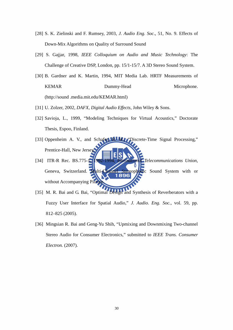
Table 1 Comparison between direct design and Multistage design.............................31

LIST OF FIGURES

Fig. 1 The waveforms of a pure-tone (a) and its truncated signal by a clipper (b)......32

Fig. 2 The frequency spectrum of only odd harmonics generated by a clipper using a

sine wave 100Hz. .........................................................................................................33

Fig. 3 The transform of a sine wave 100 Hz on the time and frequency domains by the

methods of hyperbolic tangent. (a) time domain (b) frequency domain......................34

Fig. 4 The complete Structure of virtual bass realization. ...........................................35

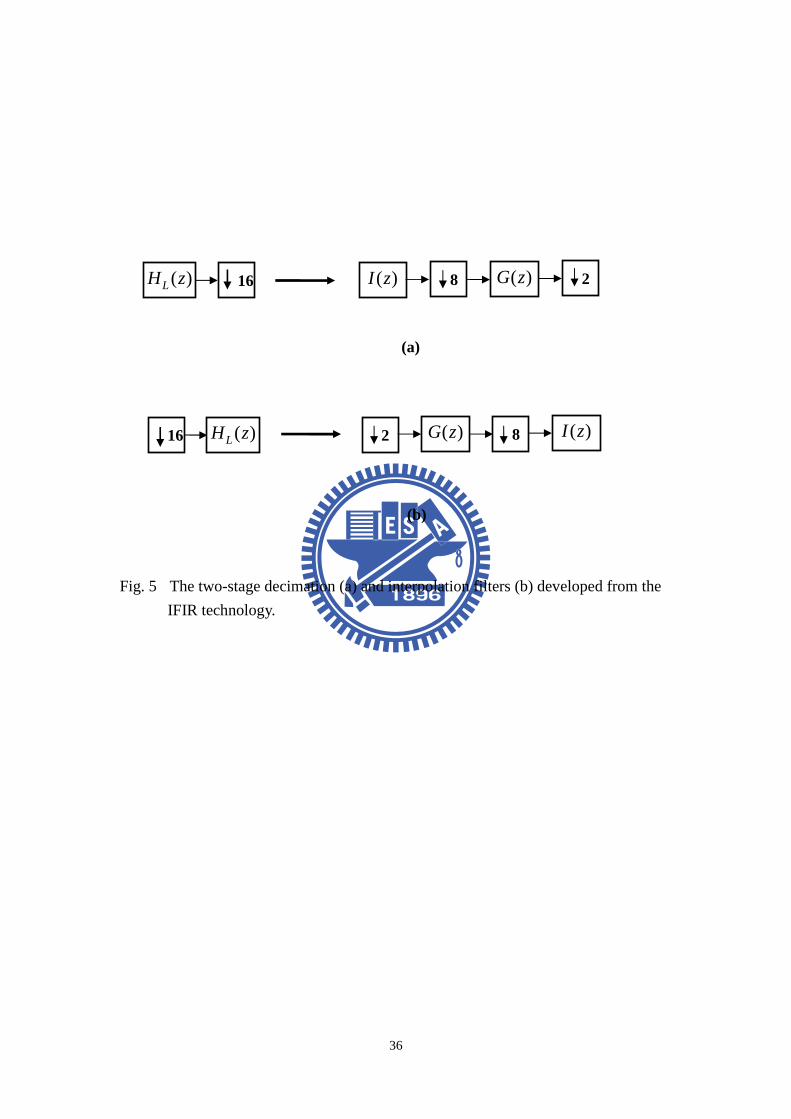
Fig. 5 The two-stage decimation (a) and interpolation filters (b) developed from the

IFIR technology. ..........................................................................................................36

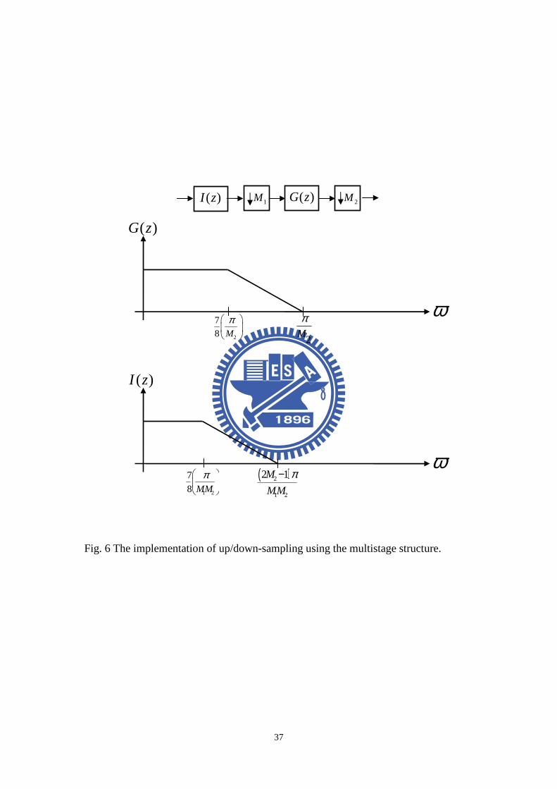
Fig. 6 The implementation of up/down-sampling using the multistage structure. ......37

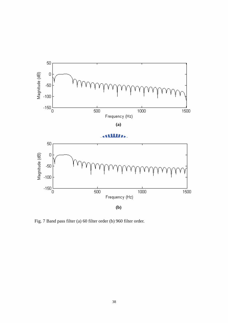
Fig. 7 Band pass filter (a) 60 filter order (b) 960 filter order.......................................38

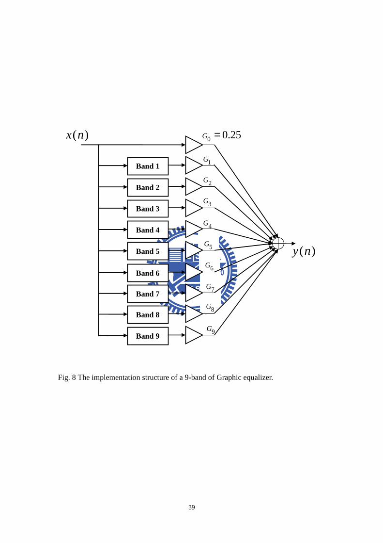
Fig. 8 The implementation structure of a 9-band of Graphic equalizer. ......................39

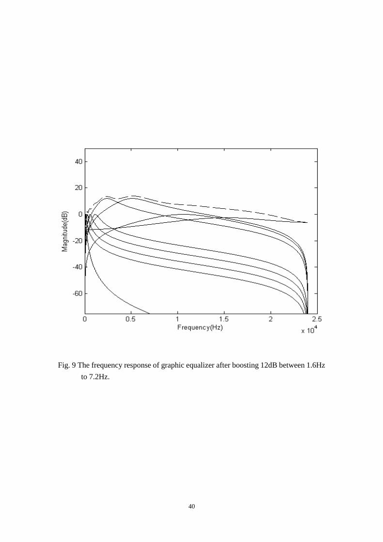
Fig. 9 The frequency response of graphic equalizer after boosting 12dB between

1.6Hz to 7.2Hz. ............................................................................................................40

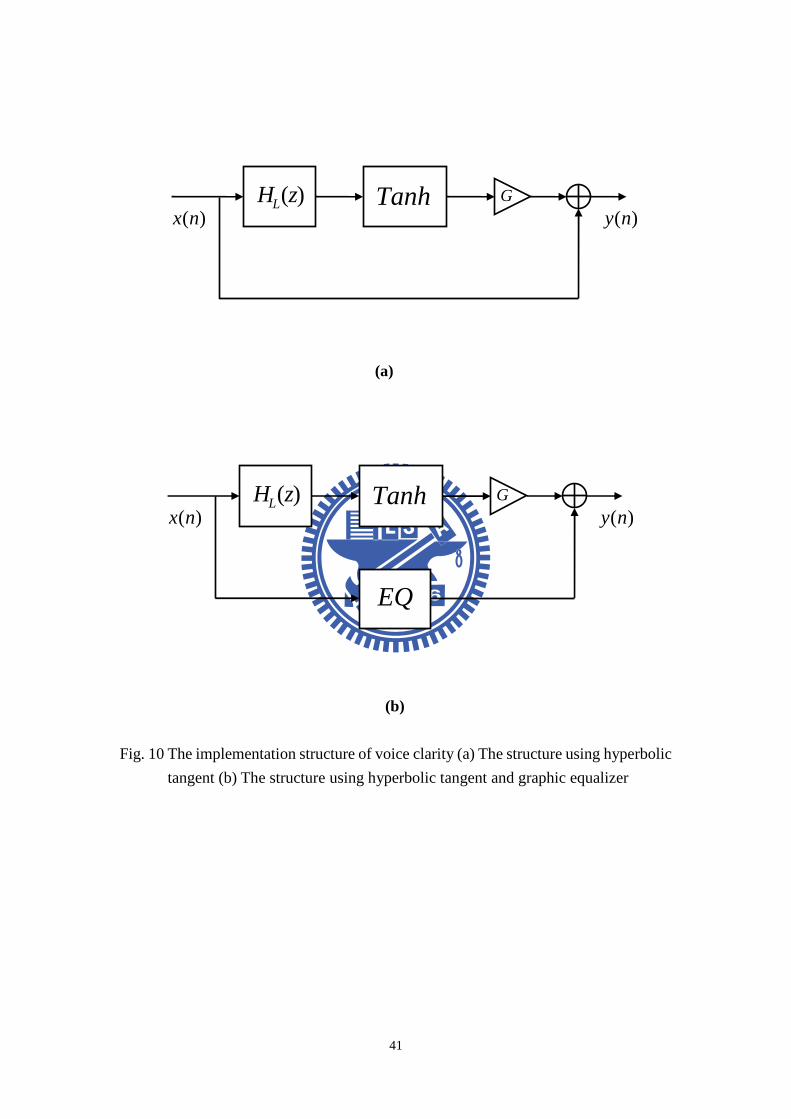
Fig. 10 The implementation structure of voice clarity (a) The structure using

hyperbolic tangent (b) The structure using hyperbolic tangent and graphic equalizer 41

VII

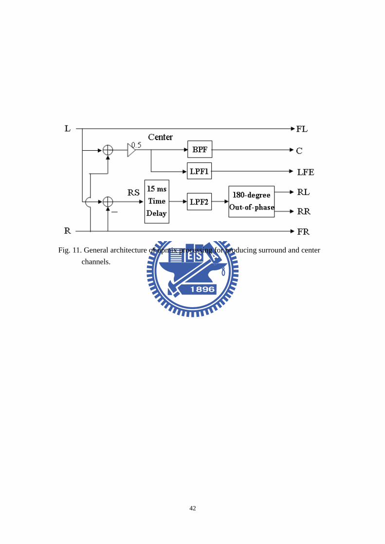
Fig. 11. General architecture of upmix processing for producing surround and center

channels........................................................................................................................42

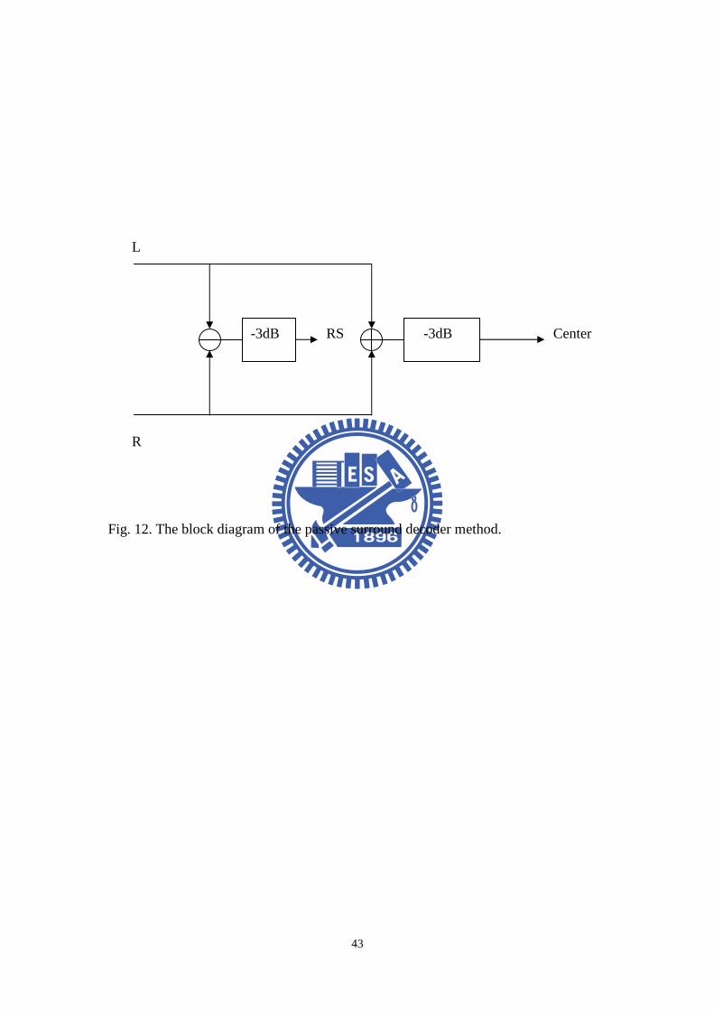
Fig. 12. The block diagram of the passive surround decoder method. ........................43

Fig. 13. Comb filter. (a) Block diagram. (b) Zero-pole plot. (c) Impulse response. (d)

Frequency response......................................................................................................45

Fig. 14. All-pass filter. (a) Block diagram. (b) Zero-pole plot. (c) Impulse response. (d)

Frequency response......................................................................................................47

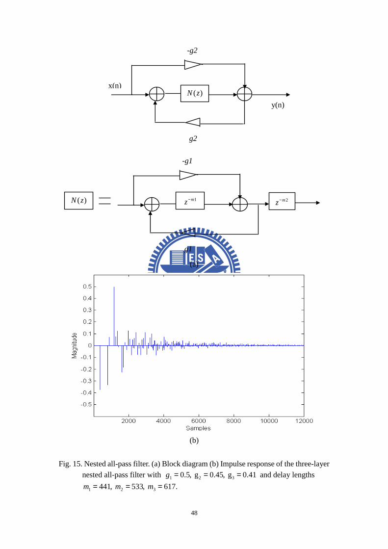
Fig. 15. Nested all-pass filter. (a) Block diagram (b) Impulse response of the

three-layer nested all-pass filter with 1 2 30.5, g 0.45, g 0.41g = = = and delay lengths

1 2 3441, 533, 617.m m m= = = ....................................................................................48

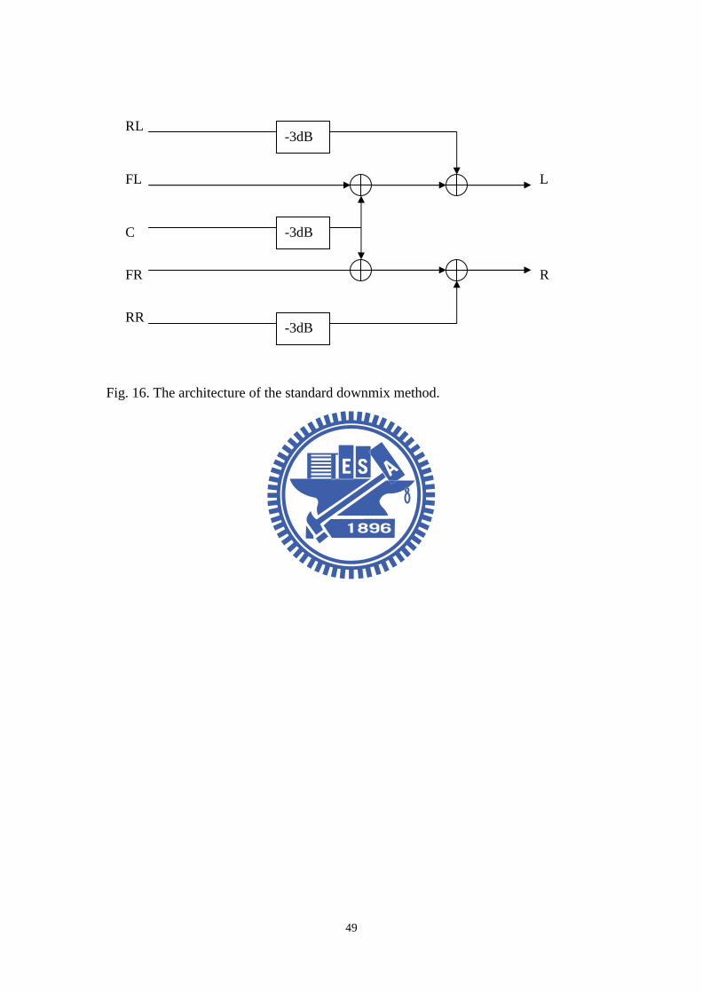
Fig. 16. The architecture of the standard downmix method. .......................................49

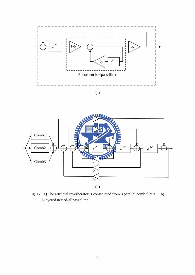
Fig. 17. (a) The artificial reverberator is constructed from 3 parallel comb filters. (b)

3-layered nested-allpass filter. .....................................................................................50

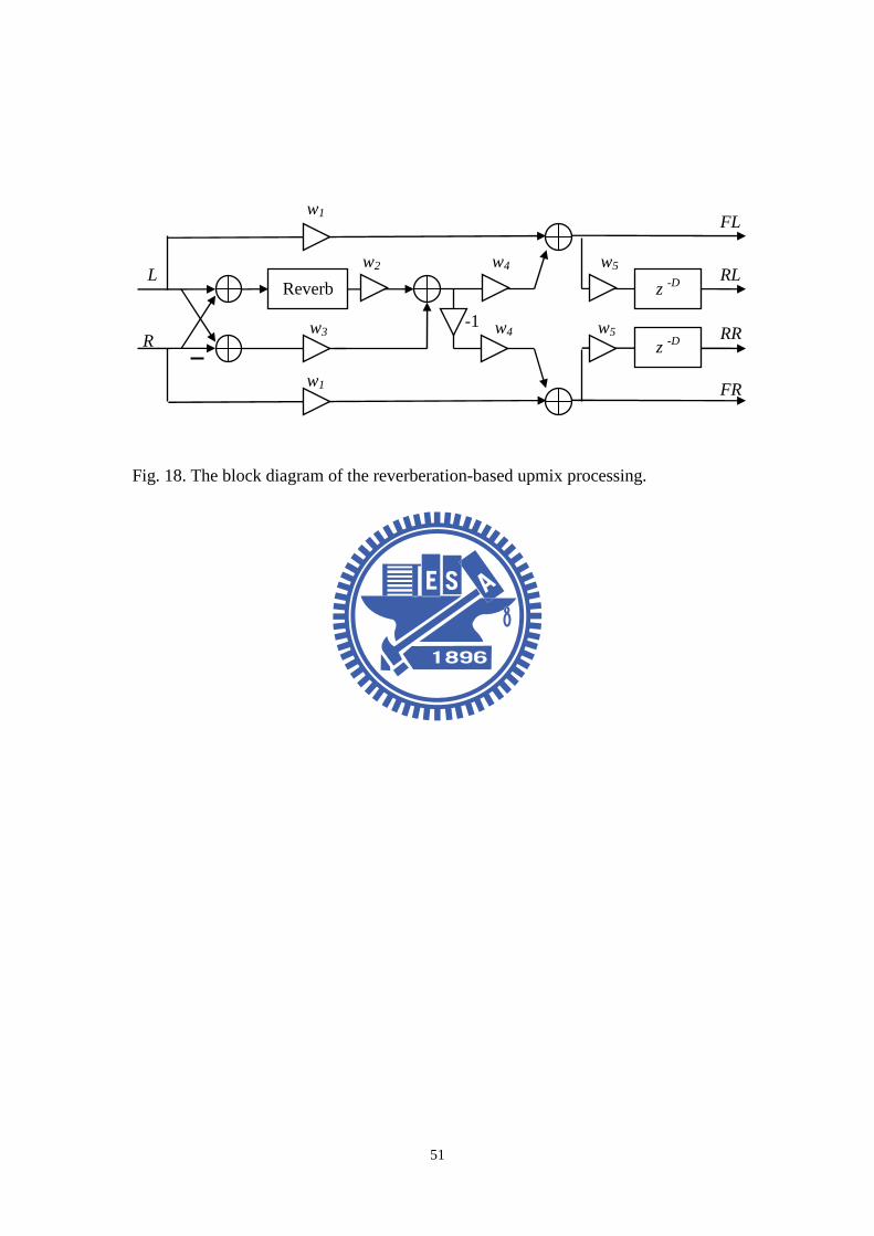
Fig. 18. The block diagram of the reverberation-based upmix processing..................51

Fig. 19. The block diagram of the standard downmix adding weighting and delay. ...52

Fig. 20 The structure of the noise level estimation system. .....................................53

Fig. 21 The block diagram of the dynamic range control system. ...........................54

Fig. 22 The RMS measurement. ..................................................................................55

Fig. 23 The static curve which is designed for using the SNR to calculate the output

gain. 56

Fig. 24 The block diagram of the adaptive gain control system. .............................57

Fig. 25 The level varying whitenoise. The upper row is the original noise. The

lower row is the estimated noise..................................................................................58

Fig. 26 The SNR which is calculated by a signal and a level varying whitenoise...59

Fig. 27 The output gain. ...........................................................................................60

Fig. 28 The experimental arrangement. ...................................................................61

VIII

Fig. 29 The waveform of case 1. The upper row is the waveform when system off.

The lower row is the waveform when system on. .......................................................62


The lower row is the waveform when system on. .......................................................63

1

1 INTRODUCTION

With rapid growth in digital telecommunication and display technologies,

multimedia audiovisual presentation has become reality for automobiles. However,

there remain numerous challenges in automotive audio reproduction due to the

notorious nature of the automotive listening environment. This study proposed

bandwidth extension (BEW) algorithms and up/downmix algorithms to create a more

ambience listening feel. And also, proposed an adaptive audio gain controller (AGC)

to enhance the listening environment.

This study presents an approach of adaptive gain controller. Two systems are

described in this study. System identification with LMS algorithm is employed to

determine the unknown plant. NLE system is used to estimate the background noise.

The DRC system is employed to obtain the output gain mapping.

With the increased proliferation nowadays of automotive audio systems, the

interior of a car is also known as a notorious listening environment due to engine,

vibration, wind and air conditioning. The background noise causes an unclear music.

This motivates the current research to develop an adaptive gain controller (AGC) to

maintain a stable signal to noise ratio (SNR) for vehicles. The AGC is also used in

speech processing [1] and hearing aids. Speech processing in an ambient noise

environment uses Artificial Neural Network (ANN) to train the weighting in different

noise conditions [2]. Another method used optimal nonlinear filtering of the

short-time spectral amplitude (STSA) envelope [3]. For the hearing aids, it is

achieved by using two control voltages to determine the gain. One changes slowly

as the input varies in level. The other comes into operation when an intense transient

occurs [4]. However, those approaches are not considered as a suitable technique for

automotive audio. The key issue is the complex processing, which limits its

implementation in practical systems. NLE achieved by LMS algorithm is

2

considering as an efficiency method for noise estimation. NLE combines DRC

approach will be presented in this study.

In order to achieve the noise estimation processing, the plant in a car

environment need to be determined. The adaptive filter [5], [6] is quite important

because its capability to track an unknown system. LMS [7]-[9] and

Recursive-Least-Squares (RLS) are two popular algorithms for adaptive filtering. In

comparison, LMS has better tracking ability, while RLS has faster convergence speed.

The LMS technique possesses the advantages of simplicity in its underlying structure,

computational efficiency, and robustness. Therefore, the LMS approach will be

presented in this study. However, we still need a DRC system [10]-[13] to

accomplish the process. DRC is described by their static and dynamic

characteristics. Static characteristics describe the DRC output response to constant

level signal. The static characteristics are typically split into four sections:

expansion, no-action, compression and limiting. The regions are separated by

threshold signal levels. Each characteristic is affected by its slope.

The proposed approaches have been implemented on a real car using a

fixed-point digital signal processor (DSP), one microphone and the loudspeakers

installed in the cars. The simulation results and the experiment setup will be

discussed in this study.

2 BANDWIDTH EXTENSION

Bandwidth extension (BWE) refers to methods that increase the frequency

bandwidth of signals. It is desired when the frequency content of the signal at some

point should be enhanced to improve audio effects or if the bandwidth of signal has

been reduced because of some economical constraints. An obvious way to

categorize various BWE methods is based on the frequency range of interest (high

3

frequency or low frequency) and where the signal bandwidth is actually extended

(physical or psycho-acoustical extension) [14]. The psycho-acoustical extension,

different to physical BWE, use no practical implementation to contain the frequency

range of interest, but exploit the property of human hearing to achieve bandwidth

extension. In this study, we described three kinds of BWE applications respectively

virtual bass (VB) and voice clarity (VC).

The first application refers to the virtual bass technology, it focuses on how to

increase bass enhancement using a loudspeaker which has no low-frequency

capability such as a cell phone. A common solution to this problem is to use

equalizers that make use of shelving filters or other electronic means, but it does not

usually get a good result. If the power amplifier and the loudspeaker are not

redesigned for the low-frequency purpose, boosting bass directly will cause

distortions or even permanent damage. To overcome the above-mentioned problems,

the virtual bass technology exploits a psycho-acoustic property of human hearing that

humans are capable of “extrapolating” the missing fundamental in the low frequency

range based on higher harmonics. The pitch-shifting algorithm of phase vocoder

can realize the concept by modifying the phase properly, and then the equal loudness

contour is exploited to adjust the loudness [15]. Instead of generating harmonics by

pitch-shifting algorithm which requires a complex calculation of phase [16],

nonlinear processing can create new bandwidth more efficiently and conveniently.

Even if the fundamental frequency is missing, it will still perceived as a residue pitch,

which in this case is sometimes called ‘virtual pitch’ or ‘missing fundamental.’

Finally, we use the implementation of multistage up/down-sampling structure to save

evaluation [17]. The second application refers to the voice clarity technology; it is

requested when the speech is not clarified enough for listening. This problem is

probably because of the low loudness of voice we want to listen or the loud

4

background music. It usually happens as someone watching movies or talking by

telephone. In this study we aim to overcome the problem by some simple

algorithms including nonlinear processing.

Because it is generally difficult to have a good low frequency loudspeaker

response with small loudspeakers, it is pertinent to ask whether other options are

available. One option is to use BWE, with the ‘extension’ taking part in the auditory

system, instead of extending the actual physical bandwidth of the signal. This

approach is to make use of the ‘missing fundamental’ effect: a special case of residue

pitch, also known as virtual pitch. We can substitute an 1f f< by a series

, 2kf k > , to evoke the residue pitch of f , while the loudspeaker does not radiate

energy at frequency f . For voice clarity, we try to make the muffled voice more

brilliant and clear by three simple algorithms. First of all, we modulate the

magnitude of certain frequency components by graphic equalizers [18] to enhance

human speech. Second, we use nonlinear process to generate high frequency

harmonics. Finally we combine aforementioned two.

2.1 NONLINEAR PROCESSING

In this chapter we describe an efficient nonlinear operation to extend frequency

bandwidth. This algorithm is convenient ways for generating harmonics signals with

odd or even harmonics. They have their own spectral characteristics and can create

different kinds of audio effects. Before explaining the applications of BWE, how the

nonlinear processing works and what the characteristics of nonlinear process are

should be described [19].

2.1.1 Clipper

A convenient way to generate a harmonics signal with only odd harmonics

5

is by means of a clipper. The clipper output signal cg in response to an input f

is

( ) | ( ) |

( ) ( )

- ( ) - ,

c

c c c

c c

f t if f t l

g t l if f t l

l if f t l

≤= > <

(1)

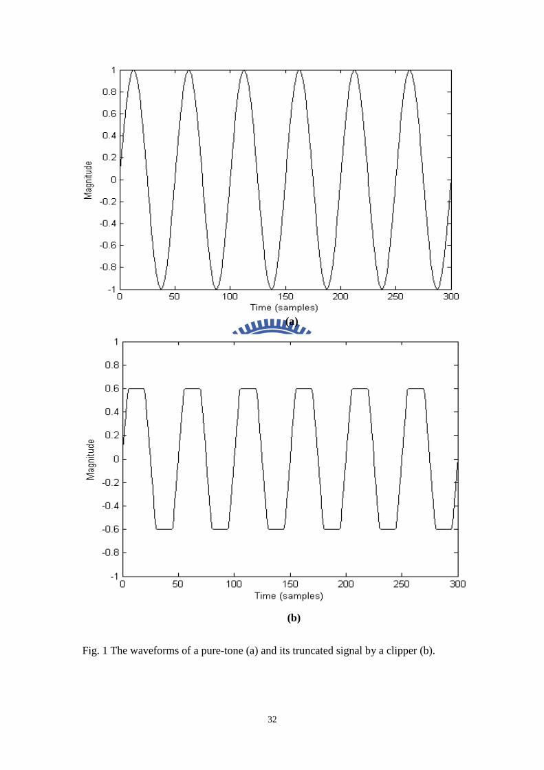
where cl is the threshold. The clipper in Fig. 1 demonstrates very good subjective

results in the low-frequency psychoacoustic BWE application. This effect due to

clipper sounds low-pitched and saturated enough, so the method is applicable to the

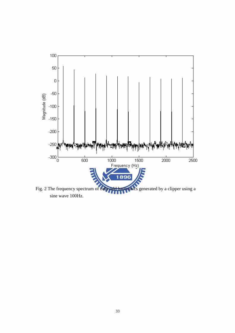
realization of virtual bass. We can get information from Fig. 2 that only odd

harmonics are created by clipper and the fundamental frequency is still preserved.

The differences between clipper and rectifier are not only positions of harmonics

generated but also preservation of the fundamental frequency. Another disadvantage

for a clipper, like a rectifier, cannot control the magnitude of harmonics.

2.1.2 Hyperbolic tangent

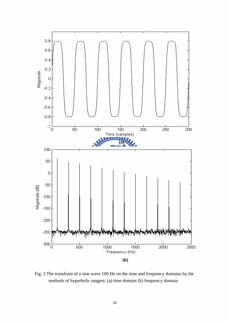
Unlike the clipper that is a “hard” clipper, the hyperbolic tangent function

shown belongs to a “soft” clipper. Fig. 3 shows the transform of a sine wave 100 Hz

on the time and frequency domains by the methods of hyperbolic tangent. We can

notice that the waveform modified by the hyperbolic tangent in Fig. 3(a) seems to be

compressed. This approach is especially suitable for dialogues but not music, which

will be validated in section 2.3. It uses a function that has a gain at low and

moderate signal levels, but attenuation at high signal levels. It is different form

ordinary compressors because it’s memoryless. That is, it is an instantaneous

compressor. During experiments, it appeared that the function where ( )x t is the

input time signal, and ( )y t is the modified output signal by hyperbolic tangent.

1 2( ) tanh( ( ))y t c c x t= (2)

6

The constant 1c determines the maximum output level and 2c determines the gain at

low signal levels.

2.2 Virtual bass

With good properties of spectral characteristics, temporal characteristics and

inter-modulation distortion [20], we choose the clipper as the method of creating

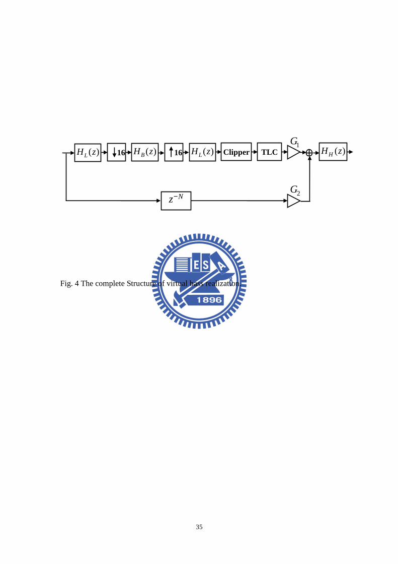
harmonics because of the best low-frequency psychoacoustic performance. Figure 4

shows the whole process of VB realization. There are two paths, the first path is the

main structure performing virtual bass, and another path just contains delay. First of

all, because of efficiency of running program, we use the method of multistage to

execute the up/down-sampling [21] to save evaluation, we chose the

up/down-sampling ratio as 16M = , and the length of original signal will decrease 16

times after operation. Figure 5 shows that the up/down-sampling process divides

into two sections, it is called the interpolated FIR (IFIR) technique [22]. We choose

8 as the first up/down-sampling ratio as well as choose 2 as the second.

In order to avoid frequency aliasing, we must design low pass filters I(z) and

G(z). Figure 6 shows how we design the multistage filter. As I(z) is concerned, if

the first up/down-sampling ratio is 1M and the second is 2M , the pass band

frequency is determined as 1 2

7

8 M M

π

when the stop band frequency is determined

as 2

1 2

(2 1)M

M M

π−, where π is the half of sampling rate. After we get the frequencies

of pass band and stop band, we can design filter on our self by matlab toolbox. One

important parameter should be noticed is the filter order, it is determined by the

equation as follows.

1, 2( )2

s p

DN

δ δπ

ω ω≈

− (3)

7

Where 1, 2( )D δ δ is a function of the peak pass-band ripple1,δ and peak stop ripple2δ ,

2π is sampling rate, sω is the stop band frequency, and pω is the pass band

frequency Form above discussions, we see that the order of ( )G z in terms of the

specifications 1δ , 2δ , pω , and sω can be written as

1, 2

1

(0.5 )2

( )gs p

DN

M

δ δπ

ω ω=

− (4)

The order of ( )I z

1, 2 1

1

(0.5 )2

2 ( )is p

D MN

M

δ δπ

π ω ω=

− + (5)

The number of MPU is approximately

1, 2 1, 2

1 1 1

(0.5 ) (0.5 )

2 2 ( ) 2 ( )g i

s p s p

N D DN

M M MM M

π δ δ π δ δω ω π ω ω

+ = +− − +

(6)

Next, between the up-sampling with down-sampling process, a band-pass filter

should be designed. The filtering signal is applied to create harmonics for virtual

bass. The bandwidth becomes 3 kHz after executing the down-sampling process, so

the band pass filter order is much less than that without doing down-sampling process.

Figure 7 shows that band pass filters (a) and (b) have almost the same performance,

however, (a) only need 60 filter order when (b) must need 960 filter taps. This is

because (a) was done by down-sampling.

Table 1 shows the comparison between a direct design without

up/down-sampling and the multistage design. We can observe that using multistage

design is more efficient in running the program.

2.2.1 Timbre Loudness Control

We use clipper, which described in Section 2.1 for creating harmonics after

8

doing up and down sampling process. Then an adjustable gain control will be used.

If this procedure is not performed, the signal modified by clipper is not amplified or

attenuated as a desired output. Instead of adjusting the loudness by equal loudness

contour, we use timbre loudness control to obtain a suitable spectrum and timbre. It

not only controls the loudness but avoids the distortion of timbre. As the equalizer is

concerned, it is similar to adjust again control over the whole bandwidth. Now the

work we do is the same purpose as the equalizer to design frequency curves which fit

with different requirements. Each step is introduced as follows.

First, we use the white noise as the input signal, and pass it along clipper and

also create a long bandwidth of harmonics. Next, we try to design a frequency curve

in frequency domain, and let the input signal be filtered off the frequency curve.

After try and error, if the output sounds like the white noise in loudness and timbre,

this frequency curve is the optimal design. Finally, after combination of the first and

second path, a high pass filter should be design for avoiding reduction of high

frequency components.

Virtual bass can also be performed on a cell phone whose loudspeaker size is

much smaller than the common one, but we must redesign the range of band pass

filter. The fundamental resonant frequency of a cell phone is almost 1000Hz when

the fundamental resonant frequency of ordinary speakers is 200Hz~300Hz

approximately. That is why I want to shift the range of band pass filter to

500Hz~1000Hz instead of 50Hz~200Hz. This process is also implemented on

automotive audio.

2.3 Voice clarity

Figure 8 shows our structure for implementing a 9 band graphic equalizer using

second order IIR filters. The feed forward path is a fixed gain of 0.25, while each

9

filter band can be multiplied by a variable gain for gain or attenuation. a and b

coefficients can be generated for the following second-order transfer function and

equivalent input and output difference equations:

1 20 1 2

1 21 2

( )( )

( ) 1

b b z b zY zH z

X z a z a z

− −

− −

+ += =− −

(7)

In theory, coefficients 1a , 2a can be found by the relation between the center

frequency nω and quality factor Q .

1

2nQ

BW

ωζ

= = (8)

where ζ is the damping ratio. After determining the nature frequencies 1ω and

2ω , the center frequency nω , bandwidth BW ,and quality factor Q will be found

rapidly. Then, we can obtain the coefficients1a , 2a . Practically, to get the

coefficients of the low-pass filters, we use MATLAB filter design toolbox. After

determining and setting up the filter type, design method, filter order, and frequency

specification, then the coefficients will be found soon.

After describing the theory of graphic equalizer, we try to implement voice

clarity by means of it. A simple way performed easily is boosting the amplitude

within proper frequency ranges to clarify human voice. Figure 9 shows the

frequency response of frequency range and magnitude for boosting. Each solid line

indicates the frequency response of each filter band in different frequency ranges, and

the dashed line represents the sum of total frequency response.

Hyperbolic tangent has been described in Section 2.2 and it is suitable for high

frequency extension and dialogues processing. Similar to graphic equalizer, a simple

way is proposed to realize voice clarity. Figure 10(a) shows the structure. Because

the magnitude of bass or low frequency is usually much louder than the one of high

frequency, let original signal pass through a high pass filter is our first step. Next,

10

use hyperbolic tangent to enhance voice or high frequency component. After

gain-adjusted, add the original music from the other path and the output is done.

In this section there is no innovation proposed, we have aforementioned methods

combined to achieve voice clarity. Figure 10(b) shows the structure.

3 INTRODUCTION OF UP/DOWNMIX PROCESSING

In recent years, computer, communication, and consumer, generally referred to

as the 3C industries are rapidly advancing. The appearance of the digital versatile disk

(DVD) and the super audio CD (SACD) has provided high quality audio and video

presentations. Also, the rapidly-developed third-generation (3G) handsets equipped

with dual-loudspeaker would have a chance to deliver high quality audio reproduction.

Using multichannel audio reproduction technology, consumers are now able to

immerse themselves seamlessly with multimedia in a theater-like environment. In

multichannel audio reproduction, upmix and downmix processing plays an important

role in many audio applications, where the number of channels of either the audio

content or the reproducing loudspeakers is limited In order to support the

compatibility with two-channel stereo signals, the upmix processing, having been

studied extensively, is employed to creating additional channels based on original

audio channels [23~27]. Since five channels have been shown to be sufficient for

simulating ambience circumstance [25], it is focused on translating the two-channel

signals into the multichannel 5.1 reproduction format in this chapter. Two general

strategies for upmix processing including the direct-ambient approach and the

‘in-the-band’ approach have been proposed [28]. The direct-ambient approach

describes that the front speakers refer to position the direct sound images and deliver

dialog, whereas the rear surround speakers refer to reproduce only diffuse and

background sound field giving rise to a sense of ambience and envelopment. The

11

‘in-the-band’ approach suggests that all loudspeakers are required to produce a sound

field in the foreground as if the listener were surrounded by sources. Furthermore, the

fact that upmix processing creates additional channels on the basis of the stereo inputs

can be achieved by using two strategies. One approach attempts to extract the

“de-correlated” part of the original audio signals, whereas another approach attempts

to produce the additional ambient reverberation that simulates the diffuse sound field

in the background. There are two methods of the first category including the passive

surround decoder method [26] and reverberation based method. And the room

response simulator mentioned before is employed to create the spaciousness and

ambience. Contrary to the upmix processing, the downmix processing refers to reduce

the number of channels due to practical reasons such as availability of loudspeakers.

In this thesis, it is focused on remixing the 5.1 audio inputs into two-channel signals

since the rendering loudspeakers are predominantly stereo in 3C products. For this

purpose, downmix can be accomplished by simple mixing or the head related transfer

function (HRTF) filtering, as in Sound Retrieval System (SRS) 3D stereo sound

system [29]. HRTF [30] is a mathematical model representing the propagation process

from a sound source to the human ears and contains spatial cues such as propagation

delay and diffraction effects due to the head, ears, and even the torso. This allows us

to create a directional impression by properly synthesizing HRTFs. As described,

upmix refers to creating additional channels of signals based on original audio

channels, whereas downmix refers to remixing multichannel audio inputs into a

decreased number of channels. However, it is noted that if the audio inputs and the

reproducing loudspeakers are both of two-channel stereo configuration, then upmix

could be concatenated with downmix to simulate a multichannel environment.

3.1 Upmix algorithm

12

In this section, five upmix algorithms including the passive surround decoder

method, the adaptive panning method, the LMS-based method, the PCA-based

method, and the artificial room simulator method are introduced. These methods

differ in how to generate the additional channels based on original audio channels. In

general, the center (C) channel corresponds to the most correlated portion between the

front right (FR) and the front left (FL) channels. A 128-tap FIR band-pass filter with

cut-off frequencies 100 Hz and 4 kHz is employed to emphasize voice and dialog for

center channel. The rear left (RL) and the rear right (RR) channels are intended to

provide ambience and environment affects. Thus, a 15 ms delay is added to the rear

channels to comply with the precedence effect. The feature of high-frequency

absorption can be simulated by filtering the rear channels with a 7 kHz cut-off,

128-tap FIR low-pass filter. In addition, the rear channels are also 180-degree

out-of-phase with one another, which helps spaciousness of the ambient field [31].

The low frequency enhancement (LFE) channel is derived from the center channel

before band-pass filtering. A 128-tap FIR low-pass filter is used to retain the signals

below 120 Hz for the LFE channel. The general architecture of the direct-ambient

upmix approach for creating the additional channels is shown in Fig. 11.

3.1.1 The passive surround decoder method

The first approach employed in this study attempts to emulate an early passive

version of the Dolby Surround Decoder [26] as shown in Fig. 12. The center channel

results from the average of the original stereo channels, whereas the rear surround

signals result from the difference. As above-stated, the center channel is band-pass

filtered to focus on the voice signal and the rear surround channels are delayed,

low-pass filtered and 180-degree out-of-phase with one another. The LFE channel is

generated by filtering the center channel by the 120 Hz low-pass filter.

13

3.1.2 Reverberation based method

The reverb has room modes such as church, small club, living room or

gymnasium. We can select the mode of Reverb filter to produce the effect of the true

environment. The algorithm of reverb can make the sound have more surround

effect. There are many important properties about the room response needed to be

considerer in the design of efficient reverberators and we will discuss them as follow.

� Echo Density

In the time domain, the echo density of a room response was defined as the

number of echoes reaching the listener per second.

34 ( )

3t

ctN

V

π= , (9)

where tN is the number of echoes, t is the time (in s), ct is the radius of the sphere

(in m) centered at the listener, and V is the volume of the room (in m3). As

differentiating with respect to t, we obtain that the density of echoes is proportional to

the square of time:

3

24tdN ct

dt V

π= . (10)

� Modal Density

The normal modes of a room are the frequencies that are naturally amplified by

the room. The number of normal modes tN below frequency f is nearly

independent of the room shape and is given as follow:

3 23 2

4

4 8f

V S LN f f f

c c c

π π= + + , (11)

where c is the speed of sound (in m/s), S is the area of all walls (in m2), and L is the

sum of all edge length of the room (in m). The modal density was defined as the

number of modes per Hertz.

14

23

4fdN Vf

df c

π≈ , (12)

Thus, the modal density of a room response grows proportionally to the square of the

frequency.

� Reverberation Time

The room effect is often characterized by its reverberation time, a concept first

established by Sabine in 1990. The reverberation time is proportional to the volume

of the room and inversely proportional to the amount of sound absorption of the walls,

floor and ceiling of the room. The Sabine’s empirical formula estimating the

reverberation time lists as follows:

60

0.163 0.163

i ii

V VT

A a S

⋅ ⋅= =∑

, (13)

where 60T is the time for the sound pressure to decay 60 dB, V is the volume of the

room (in m3), iS and ia are the surface of a material employed in the room and the

associated absorption coefficient, and the total absorption of material is A. Since

most materials of surface in a room are more absorptive at high frequencies, the

reverberation time of a room is also decreases as the frequency increases. The

reverberation time is used for estimating the degree of sound absorption in a room.

� Energy Decay Curve (EDC) and Energy Decay Relief (EDR)

The method to determine the reverberation time of a measured room is finding

the time when the associated sound pressure attenuate 60 dB in the plot of the EDC,

Schoroeder proposed in 1965. He suggested integrating the impulse response of the

room to get the room’s energy decay curve.

2

2

( )

( )

( )

t

t

h d

EDC t

h d

τ τ

τ τ

∞

∞=∫

∫, (14)

where ( )h τ is the impulse response of the room. Later, Jot proposed a variation of

15

the EDC to help visualize the frequency dependent natural of reverberation called the

energy decay relief ( , )EDR t ω . The EDR represents the reverberation decay as a

function of time and frequency in a 3D plot. To compute it, we divide the impulse

response into multiple frequency band and compute Schoroeder;s integral for each

band.

� Modeling Early Reflection

A room response from a source to a listener can be obtained by solving the wave

equation also known as the Helmholtz equation. However, it can seldom be

preformed in an analytic form and is more complex in solving. Therefore, the

solution must be approximated and there are three different approaches in

computational modeling of room based on acoustics [32]. The ray-based methods,

including the ray-tracing and the image-source method, are the most often used

modeling techniques. With the assumption of the wavelength of sound is small

compared to the area of surface in the room and large compared to the roughness of

surface, all phenomena due to the wave nature, such as diffraction and interference,

are ignored. The image-source method examines the effects of an acoustic source in

a room with corresponding sources located in image rooms with reflecting boundaries.

Each of the infinite sources will produce attenuated, filtered and delayed version of

the original acoustic input. The total effects can be summed to produce a transfer

function or a FIR filter.

� Modeling Late Reverberation

There are two approaches to model late reverberation, the FIR-based and

IIR-based methods. Implementing convolution using the direct form FIR filter is

extremely inefficient when the filter size is large. Typical room responses are

several seconds long, which at a 44.1 kHz sampling rate would translate to a huge

number of points filter. One method to deal with the large size FIR filter is using an

16

algorithm based in the Fast Fourier Transform (FFT) block convolution [33]. The

second method is try to model the late reverberation of a room based on some

IIR-filters, comb and all-pass filters, Schoroeder proposed first in the early 1960’s, or

a mixture of them. The details of comb filter and all-pass filter will be discussed in

the next section.

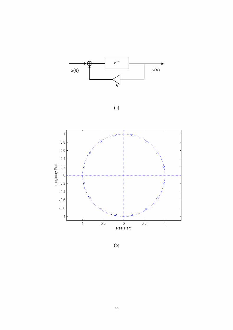
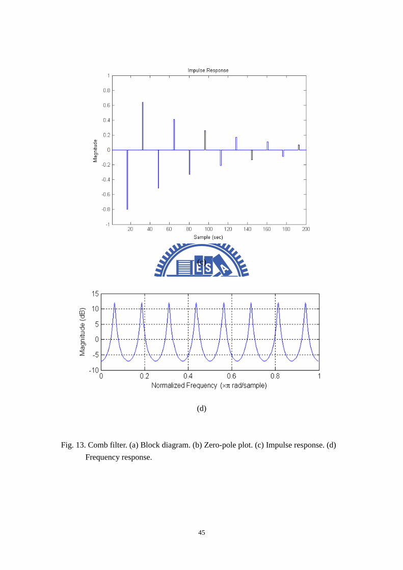
� Comb Filter

The block diagram of comb filter shown in Fig. 13 consists of a single delay

line of m samples with a feedback loop containing an attenuation gaing . The z-

transform of the comb filter is given by:

( )1

m

m

zH z

gz

−

−=−

. (15)

Note that to achieve stability, g must be less than unity. The time response of

this filter is an exponentially decaying sequence of impulse spaced m samples apart.

This is good for modeling reverberation because real room have a reverberation tail

decaying somewhat exponentially. However, the echo density is really low, causing

a “fluttering” sound on transient input. The pole-zero map of the comb filter shows

that a delay line of m samples creates a total of m poles equally spaced inside the unit

circle when it is stable. Half of the poles are located between 0 Hz and the Nyquist

frequency / 2sf f= Hz, where sf is the sampling frequency. That is why the

frequency response has m distinct frequency peaks giving a “metallic” sound to the

reverberation tail. We perceive this sound as being metallic due to hearing the few

decaying tones that correspond to the peaks in the frequency response.

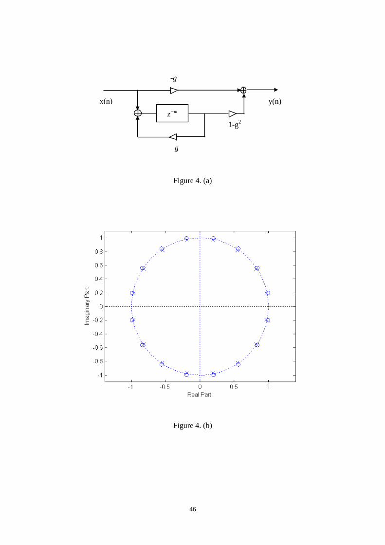
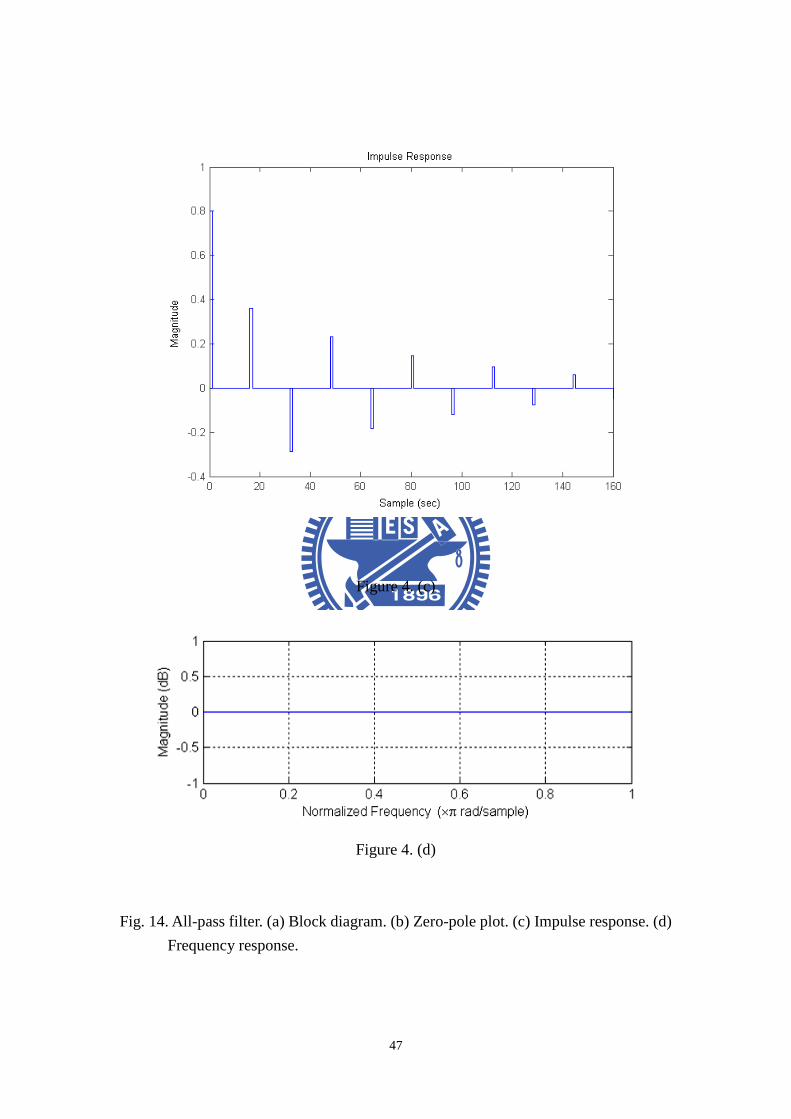
� All-pass Filter

Because the poor performance of frequency response of a comb filter, Schroeder

modified to provide a flat frequency response by mixing the input signal and the comb

filter output as shown in Fig. 14. The resulting filter is called an allpass filter

17

because its frequency response has unit magnitude for all frequencies. The

z-transform of the all-pass filter is given by:

( )1

m

m

z gH z

gz

−

−

−=−

. (16)

The poles of the all-pass filter are thus the same as for the comb filter, but the

all-pass filter now has zeros at the conjugate reciprocal locations.

And the response of an all-pass filter sounds quite similar to the comb filter,

tending to create timbre coloration.

� Nested All-pass Filter

To achieve a more natural-sounding reverberation network, it would be desirable

to combine the unit filters to produce a buildup of echoes, as it would occur in real

rooms. One solution to produce more echoes is cascading multiple all-pass filters

which Schroeder had experimented with reverberators consisting of 5 all-pass filters

in series. Schroeder noted that these reverberators were indistinguishable from real

rooms in terms of coloration, which may be true with stationary input signals, but

other authors have found that series all-pass filters are extremely susceptible to tonal

coloration, especially with impulsive inputs. Gardner proposed reverberators based

on a “nested” all-pass filter, where the delay of an all-pass filter is replaced by a series

connection of a delay and another all-pass filter. The block diagram and its impulse

response are shown in Fig. 15(a), where the all-pass delay is replaced with a system

function ( )N z , which is all-pass. Then the transfer function of this from is written:

1

1

( )( )

1 ( )

N z gH z

g N z

−=−

. (17)

The advantage of using a nested all-pass filter can be seen in the impulse

response in Fig. 15(b). Echoes created by the inner all-pass filter are recirculated to

itself via the outer feedback path. Thus the echo density of a nested all-pass filter

increases with time, as in real rooms.

18

3.2 Downmix algorithm

The creation of DVD and SACD causing a revival of multichannel audio has

carried out the high quality audio performance. However, many applications such as

personal computer multimedia, portable audio products, TVs and cell phones are

equipped with only stereo loudspeakers. Thus, downmix processing is necessary to

downmix a multichannel content, e.g., 5.1 into two channels. Two downmix

techniques will be presented as follow.

3.2.1 The standard downmix method

The method suggested in the ITU standard [34] refers to mix the multichannel

signals with simple gain adjustment. The architecture of the standard downmix

method is shown in Fig. 16. In this method, the center channel is attenuated by 0.71

(or 3 dB) and mixed into the front channels. Similarly, the rear left and the rear right

surround channels are attenuated by 0.71 and mixed into the front left and the front

right channels, respectively. That is,

0.71 0.71

0.71 0.71

L FL C RL

R FR C RR

= + × + ×= + × + ×

. (18)

Nevertheless, depending on the rendering loudspeaker system, the LFE channel can

be mixed into the front channels as an option.

3.2.2 The HRTF-based downmix method

In addition to the aforementioned standard downmix method, the approach

employing the HRTF technique is included in this thesis. The HRTF technique allows

us to create a directional impression so as to enhance to the multichannel reproduction

in the downmix processing. In the HRTF-based method, no special processing is

applied to the front left and the front right channels. The center, the rear left, and the

rear right channels are filtered by the corresponding HRTFs at 0� , 110+ � , and

19

110− � , respectively, before mixing with the front channels. The HRTF database

implemented by using 128-tap FIR filters is from the website of the MIT media lab

[30]. Thus, the front right channel, front left channel, rear right channel and rear left

channel can felt more directional.

3.3 Two-channel inputs for automotive audio

In traditional automotive audio, the left-input signals are fed to both front-left

and rear-left loudspeakers, and the right-input signals are fed to both front-right and

rear-right loudspeakers. Balance of the left and right as well as the front and the rear

can usually be adjusted. The problem with this approach is that the front and rear

channels are too correlated to create natural-sounding surround effects. The paper

seeks to develop upmixing algorithms for extending two-channel input to four

channels. Upmixing can generally be achieved by two categories of approaches.

One approach is decorrelation-based methods, e.g., Prologic II and Logic 7, etc.

Another approach is reverberation-based method that is found to be very effective in

producing sense of space, especially for small space [35]. In a previous subjective

listening test [36], the reverberation-based methods outperformed the

decorrelation-based methods in ambient surround effects. Thus, only the

reverberation-based upmixing method is adopted in the following discussion.

Here developed as an alternative solution to the problem of automotive surround

audio. Figure 18 shows the block diagram of this method, in which concatenated

upmixing and down mixing processing is required. In the study, weightings (0.65)

and delay (20 ms) are used. The upmix module is described here, where

two-channel input signals are extended to four channels by the reverberation-based

upmixing algorithm and then inverse filtered to produce the outputs. An artificial

reverberator is employed to produce the rear surround channels. The artificial

20

reverberator is constructed from 3 parallel comb filters shown in Fig. 17(a) and a

3-layered nested-allpass filter shown in Fig. 17(b). The difference between the left

and right input signals is mixed into the rear channel to enhance ambience. The

rear-left and rear-right channels are made180° out of phase.

With the upmixed signals, downmixing can be done by two methods. One is only

done by standard weighting and summation to produce the two-channel outputs.

The other one is done by HRTF downmixing, which is mentioned before.

3.4 5.1-channel inputs for automotive audio

Another category of automotive surround processors that accepts 5.1 input

signals from Dolby Digital or DTS decoder in DVD players will be presented in this

section.

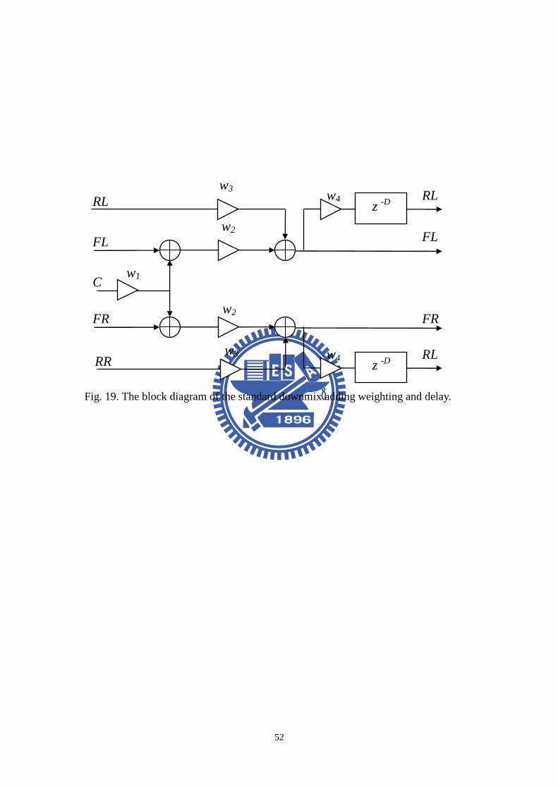
The strategy here is developed for inputs in 5.1 formats, as depicted in the block

diagram of Fig. 19. In the method, the center channel is first mixed into the front

two channels and then the ipsi-lateral channels are summed to produce the two frontal

channels. Next, the frontal channels are weighted and delayed to produce the rear

channels. The downmixing methods are the same as the above method. When the

downmix processing is done, the surround channels are produced by the weighting

and delay of front channels.

4 ADAPTIVE AUDIO GAIN CONTROLLER BASED ON NOISE LEVEL

ESTIMATION

Noises resulting from the engine, panel vibration, tire, wind, pass-by traffic, air

conditioning, etc., could significantly degrade the music listening quality in a car.

This paper proposes a new system that makes use of a Noise Level Estimator (NLE)

in tandem with s Dynamic Range Controller (DRC) to adaptively adjust the gain of an

automotive audio system. A microphone is required in the NLE as the senor to pick

21

up music signals corrupted with cabin noise. The background noise level is

estimated adaptively using the Least-Mean-Squares (LMS) algorithm. The a priori

Signal-to-Noise Ratio (SNR) is calculated based on the noise level estimated above.

From the SNR, the gain of the audio input can be adjusted dynamically, with the aid

of a static curve. The system has been implemented by using a Digital Signal

Processor (DSP) on a real car. Results obtained from simulations and experiments

reveal that the proposed system is capable of regulating the audio volume on the fly,

in response to the noise in the car cabin.

4.1 Noise level estimation by least mean square method

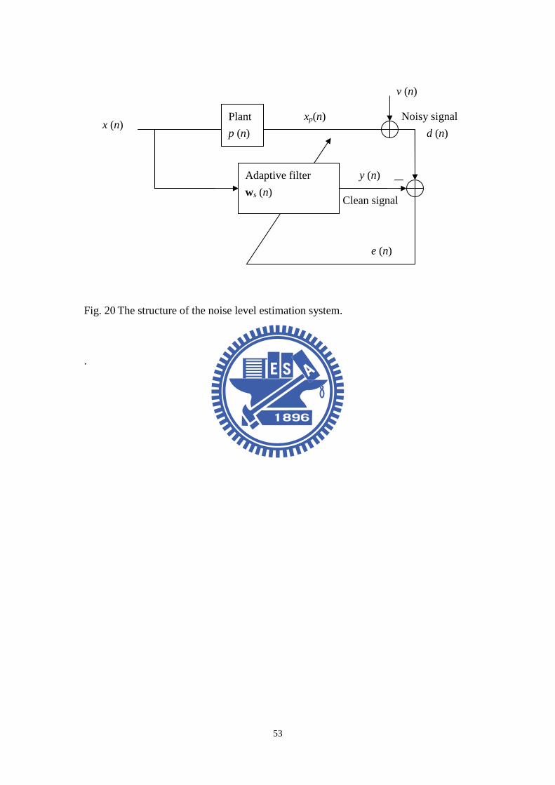
System identification is the procedure of analyzing an unknown system. The

well-known method to achieve the identification processing is the LMS algorithm [7].

The system structure is shown in Fig. 20, where ( )x n is the input signal and

( )px n is the desired signal. The desired signal can be determined by the optimal

coefficient ( )sw n , which is obtained by minimizing the error signal( )e n . Basically,

the system learns from its environment is designated as an adaptive filter where the

filter coefficients are updated according to

( 1) ( ) ( ) ( ) s s sn n e n nµ+ = +w w x , (19)

where

( ) [ (1) (2) ... ( )]Ts n w w w N=w (20)

is the filter coefficients vector of dimension 1N × .

( ) [ ( ) ( -1)... ( - 1)]Tn x n x n x n N= +x (21)

is the input signal vector of dimension 1N × .

And sµ is the step size. The stability of such a closed-loop system is governed by

the adaptation parameter and it should satisfy the condition

22

2

0 sxL P

µ< <⋅

, (22)

where L is filter length and xP is the total power of( )x n . The total power of

( )x n is the sum of mean-square value of the input signal. When sµ is small, it takes

more time to converge to a minimum error, and vice versa.

Applied in a noisy condition, system identification is a pre-processing for NLE.

As the unknown plant is determined, the noise can be estimated from the difference

between noisy path and noise-free path. See Fig. 20, ( )x n is the input signal,

( )px n is the signal through a plant and receive from a microphone. ( )v n is the

background noise. The above system can be written as

( ) ( ) ( )pd n x n v n= + . (23)

The FIR estimator for the system is defined by

s( ) = ( ) ( )y n n nx w . (24)

According to the processing of system ID the optimum parameters of the unknown

plant can be determined by minimizing the Mean-Square-Error (MSE).

2min [ ( )]IDE e n , (25)

where [ ]E ⋅ denotes the expectation operator. And ( )IDe n is defined as follow

( ) ( ) ( ) ( ) ( ) ( )ID p p se n x n y n x n n n= − = − x w . (26)

In the case, the estimation error ( )NLEe n is expressed as the difference between the

measured and the predicted system output,

( ) ( ) ( ) ( ) ( ) ( ) ( )NLE p se n d n y n x n v n n n= − = + − x w , (27)

The system setup is illustrated in Fig. 20. Here, ( )v n and ( )px n are assumed to

be uncorrelated. When the signal ( )px n is determined and equal to the output

( )y n then ( )NLEe n is equal to ( )v n .

23

4.2 Dynamic range control

DRC of audio signal is used in many applications to match the dynamic

behavior of the audio signal to different requirements. While recording, DRC

protects the AD convector from overload or it is used in the signal path to optimally

use the full amplitude range of a recording system. When reproducing music and

speech in a car, the dynamics have to match the noise characteristic inside a car. A

DRC is an automatic gain control device which modifies the dynamic range without

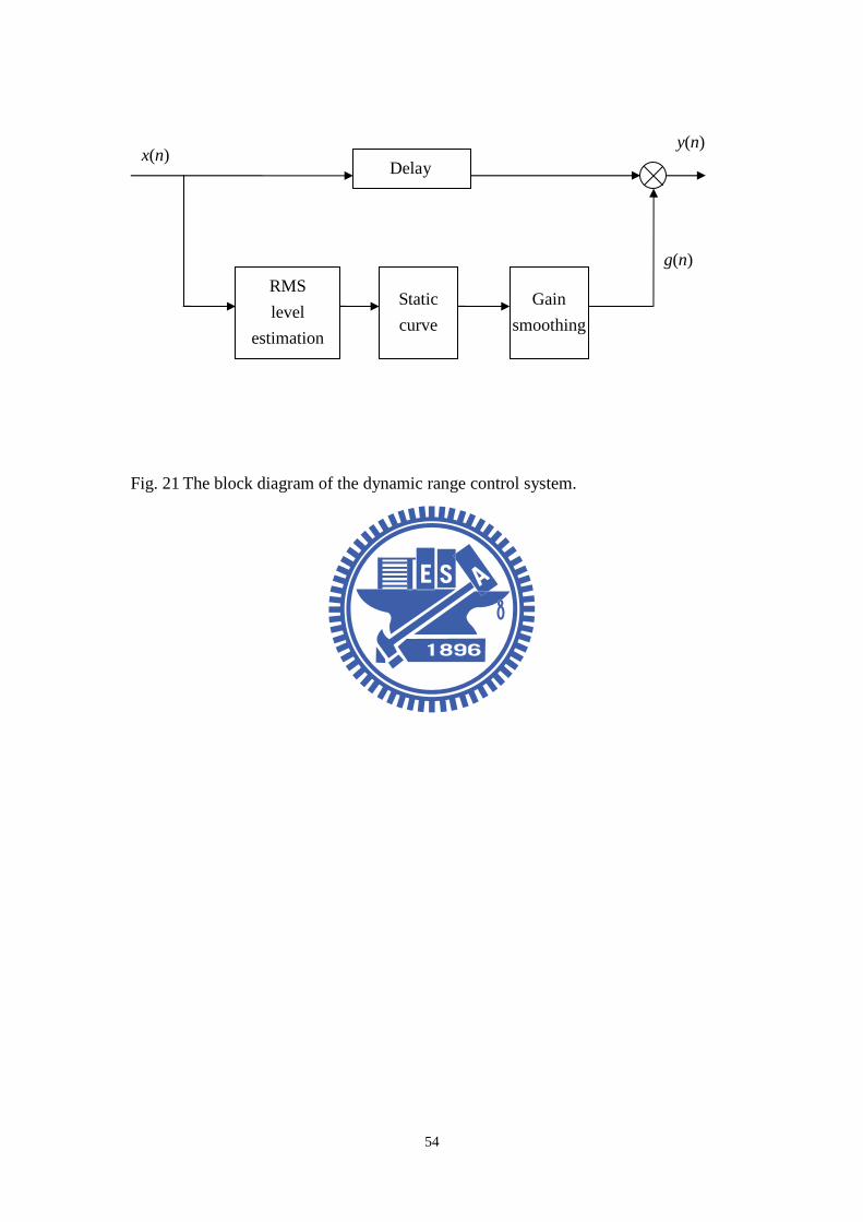
introducing perceptible distortion. Fig. 21 shows a block diagram of DRC system.

After measuring the level of input signal x, the output signal y is affected by

multiplying the delayed input signal by a factor ( )g n according to

( ) ( ) ( )y n g n x n D= ⋅ − , (28)

where D is the delay sample for non-process path and( )g n is a gain factor that

obtained according to the input level. Level measurement plays an important role in

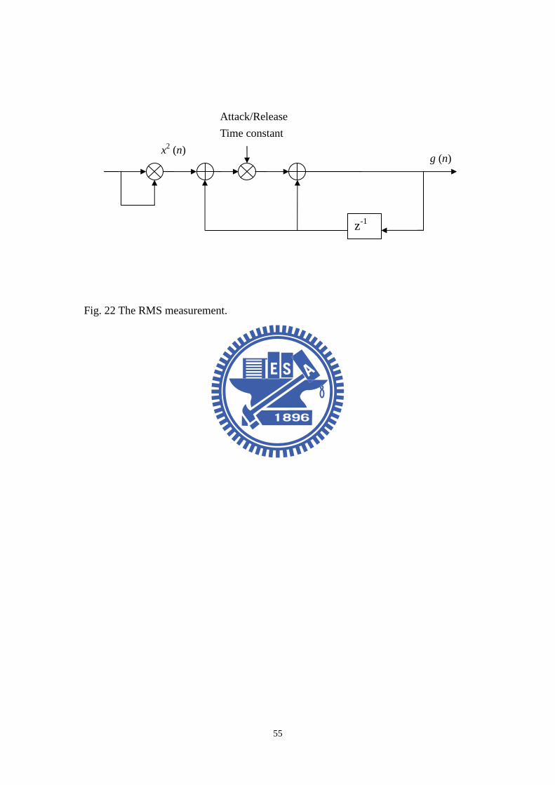
DRC. The rapidity of DRC depends also on the measurement of RMS values [10].

The RMS measurement is shown in Fig. 22. Uses the square of the input and

performs averaging with a first-order low-pass filter. The difference equation is

given by

2( ) (1 ) ( 1) ( )RMS RMSx n x n x nτ τ= − ⋅ − + ⋅ , (29)

where ( )RMSx n is signal through the RMS measurement processing and τ is the

average coefficient. The transfer function is

1

( )1 (1 )

H zz

ττ −=

− −. (30)

The system also serves to smooth the gain multiplier by using the attack coefficient

and release coefficient. The attack coefficient AT (attack time) and release

coefficient RT (release time) is obtained by comparing the input signal and the

previous sample. Then the system determines whether the control factor is in the

24

attack or release status. If the input signal is lager than the previous signal, then

system gives the attack coefficient AT. If the input signal is smaller than the

previous signal, then system gives the release coefficient RT.

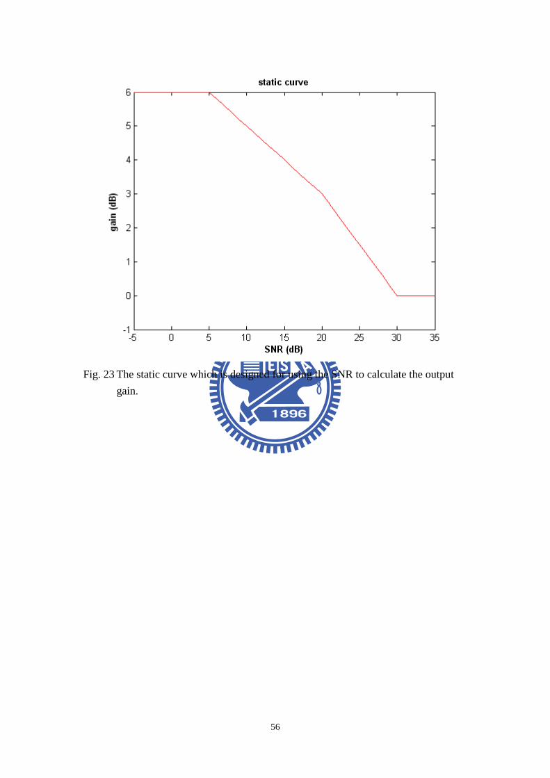
The relationship between input level and weighting level is defined by static curve.

In this paper, the output level and the weighting level are given as functions of the

input SNR level g[dB] = f(SNR[dB]). Fig. 23 shows a static curve which varies with

the SNR. According to the static curve, the limiter threshold is 6 dB. The output

gain is limited when the SNR level exceeds the limiter threshold. All SNR levels

less than this threshold lead to a constant output gain 6 dB. The SNR between 5~25

dB represents an amplifier, and has two slopes. The slope between 5 dB SNR to 20

dB SNR is 0.2. The slope between 20 dB SNR to 30 dB SNR is 0.3. Both the two

parts are compressor curves. The SNR exceeding 30 dB leads to a constant gain 0

dB.

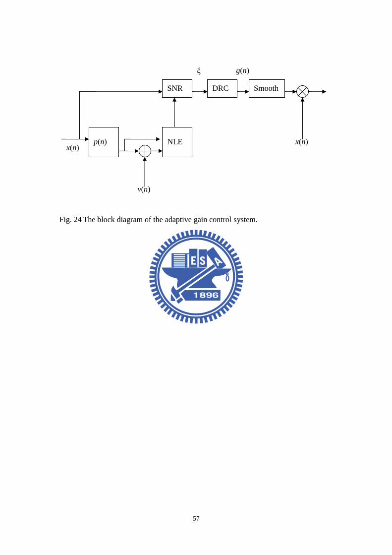
4.3 Integration of NLE and DRC modules

The two systems mentioned above have their own specific applications. This

paper is focusing on how to improve the listening quality in a car environment. We

combined NLE system and DRC system to deal with the noisy condition in a car.

The system block diagram is shown in Fig. 24. Take the NLE system as first step,

the optimal parameter of the adaptive filter is obtained from eq. (19). Then according

to eq. (25), eq. (26) and (27) the background noise level can be accurately estimated

from a noisy signal. The signal then goes through RMS level measurement and

turns into RMSx by eq. (29). Because the purpose is trying to adaptively adjust the

output signal gain according to background noise, the signal to noise ratio (SNR) is an

important factor. Use the power of background noise level and the power of signal

level to calculate a priori SNR, where a priori SNR is given by

25

2

2

px

vζ = , (31)

where px is the signal through plant and v is background noise.

As mentioned before, the static curve needs to be designed in advance. Based

on a priori SNR and static curve, the output gain mapping can be determined.

4.4 System simulation and experimental investigation

Simulations and experiments are undertaken to validate the NLE and DRC

modules proposed in the paper.

A. Simulations

We evaluated the proposed algorithm by performing a system simulation of the

adaptive gain controller system. As the proposed processing mentioned before, the

adaptive filter is used to track the plant when the NLE system is working.

According to the NLE system structure shown in Fig. 20, the filter coefficients are

adaptively calculated from eq. (19), and the step size is equal to 0.45. From eq. (19),

(25) and eq. (26) the optimal parameter is determined when the error is converging.

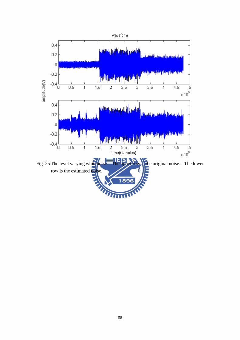
In Fig. 20, the program input ( )x n is an 8-second music excerpt and ( )v n is

an 8-second background noise. The background noise is a level varying whitenoise.

When the unknown plant is determined, the background noise can be calculated by

(27). See Fig. 25, the upper row is the original background noise and the lower row

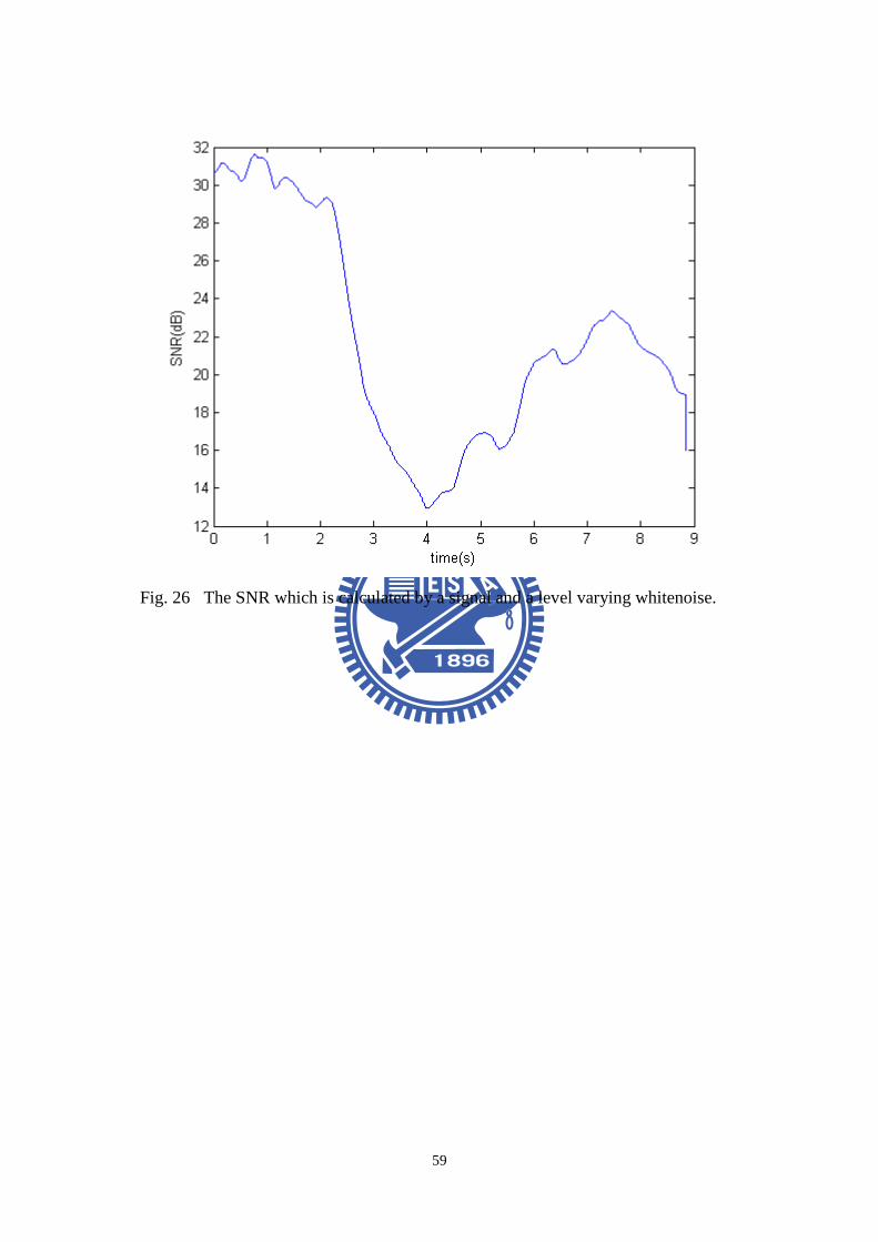
is the estimated background noise. After the background noise is estimated, the

system then calculates the a priori SNR by (30). Fig. 26 shows the SNR curve, this

is calculated by the signal and the background noise which is varying in 3 different

levels. From Fig. 26, the SNR fluctuates between 12 dB to 31 dB. There is an

obvious notch from the 2nd to the 6th second. According to the purposed algorithm,

the output gain curve should obtain a higher gain when the SNR curve is falling to a

26

notch. The relationship between input SNR level and gain level is defined by a static

curve. The static curve has described in section III. With the aid of the static curve

and the calculated SNR curve, the output gain can be obtained. Fig. 27 shows the

output gain curve. When the SNR is small, the system gets a higher gain. When

the SNR is high, the system gets a lower gain.

B. Experiments

Fig. 28 shows the experimental arrangement. Experiments were conducted in

an Opel Vectra 2-liter sedan equipped with a multichannel audio decoder, and four

loudspeakers (two mounted in the lower panel of the front door and two behind the

back seats). In this section, the adaptive gain controller based on one-microphone

noise level estimation is examined. The algorithms were implemented on the

platform of a fixed-point DSP, ADI BF-533, of Analog Device semi-conductor. The

GRAS 40AC microphone with GRAS 26AC preamplifier was used for receiving the

signal and the background noise. The position of the microphone is located at the

center of the car.

The experiments were implemented by the following process. We turned on the

system and microphone first. Through the DSP board, the program music was

played form the right channel. With the ambient noise and the signal, the

microphone picked up the noisy signal. The NLE system dealt with the noisy signal.

As soon as the adaptive filter approximated the plant, the background noise level can

be estimated. After the noise level is estimated, the system would output gains for

the input signal to maintain the SNR. There are two cases in this experiment. Case

1 used the ambient noise in a moving car. Case 2 used the level varying whitenoise.

Both the noises were played from the left channel. Fig. 29 shows the experimental

result of case 1. Fig. 30 shows the result of case 2. The upper row is the waveform

when the system is off. The lower row is the waveform when the system is on. In

27

case 1, the output signal changes moderate because the noise does not have clear level

changing. In case 2, the result shows the output signal has obvious level changing

with the level varying whitenoise.

5 CONCLUSIONS

In this study, we have proposed an adaptive gain control system based on

one-microphone noise level estimation. In this system, we select single channel

music and a background noise recorded from a moving car to be the test signal.

When system ID, the unknown plant can be accurately tracked by LMS algorithm.

The background noise level is then obtained from NLE system. Referring to the

theory of DRC, we propose a static curve which uses SNR to determine the output

gain.

We have evaluated the proposed algorithm by performing a system simulation,

DSP implementation and experiment of the adaptive gain control system. The

experimental results show that the system can dynamically adjust the audio gain when

the background noise is varying.

REFERENCE

[1] H. Drucker, “Speech Processing in a High Ambient Noise Environment,” IEEE

Trans. Audio and Electroacoustics, vol. 16, no. 2, pp. 165-168, 1968.

[2] M. Heckmann, F. Berthommier and K. Kroschel, “Noise Adaptive Stream

Weighting in Audio-Visual Speech Recognition,” EURASIP. Applied Signal

Processing, vol. 11, pp. 1260-1273, 2002.

[3] D. E. Tsoukalas, J. N. Mourjopoulos and G. Kokkinakis, “Speech Enhancement

Based on Audible Noise Suppression,” IEEE Trans. Speech and Audio Processing, vol.

28

5, no. 6, pp. 497-514, 1997.

[4] B. C. J. Moore, B. R. Glasberg and M. A. Stone, “Optimization of a slow-acting

automatic gain control system for use in hearing aids,” British Journal of Audiology,

vol. 25, no. 3, pp. 171-182, 1991.

[5] S. Haykin, Adaptive Filter Theory, Englewood Cliffs, NJ: Prentice-Hall, 2002.

[6] S. Haykin, “Adaptive Filters,” IEEE Signal Processing Magazine, vol. 16, pp. 20.

[7] N. Kalouptsidis and S. Theodoridis, Adaptive System Identification and Signal

Processing Algorithm, Englewood Cliffs, NJ: Prentice-Hall, 1993.

[8] A. K. Pradhan, A. Routray, and A. Basak, “Power System Frequency Estimation

Using Least Mean Square Technique,” IEEE Trans. Power Delivery, vol. 20, no. 3, pp.

1812-1816, 2005.

[9] A. Feuer and E. Weinstein, “Convergence analysis of LMS filters with

uncorrelated Gaussian data,” IEEE Trans. Acoust., Speech, Signal Processing, vol. 33,

no. 1, pp. 222–229, 1985.

[10] G. W. McNally, “Dynamic Range Control of Digital Audio Signals,” J. Audio

Eng. Soc., Vo1.32, no 5, pp. 316-327, 1984.

[11] A. T. Schneider and J. V. Hanson, “An Adaptive Dynamic Range Controller for

Digital Audio,” IEEE Pacific Rim Conference on Communication, Computers and

Signal Processing, 1991.

[12] M. H. Hayes, Statistical Digital Signal Processing and Modeling, New York:

Wiley, 1996.

[13] U. Zolzer, Digital Audio Signal Processing, New York: Wiley, 1995.

[14] E. Larsen and R. M. Aarts, and O.Ouweltjes. “A unified approach to low- and

high-frequency bandwidth.” the 115th AES convention, New York, Audio

Engineering Society, 2003.

[15] M. R. Bai and W. C. Lin, “Synthesis and Implementation of Virtual Bass

29

System with a Phase-Vocoder Approach,” J. Audio Eng. Soc. vol. 54,

pp.1077-1091, 2006.

[16] T. H. Andersen and K. Jensen, “Importance and Representation of Phase in the

Sinusoidal Model,” J. Audio Eng. Soc., vol. 52, no.11, pp.1157-1169, 2004.

[17] R. E. Crochiere and L. R. Rabiner, Multirate Digital Signal Processing.

Prentice-Hall, Englewood Cliffs, NJ, 1983.

[18] J. Tomarakos, D. Ledger, Using The Low-Const, High Performance

ADSP-21065L Digital Signal Processor For Digital Audio Applications, 1998.

[19] E. Larsen, R. M. Aarts and M. Danessis, “Efficient high frequency bandwidth

extension of music high frequency bandwidth extension of music and speech,”

the 112th AES convention, Munich, Germany, May 2002, 10-13.

[20] E. Larsen and R. M. Aarts, Audio Bandwidth Extension, John Wiley, West

Sussex, England, 2004.

[21] P. P. Vaidyanathan, Multirate Systems and Filter Banks, Prentice-Hall,

Englewood Cliffs, NJ, 1993.

[22] A. V. Oppenheim and R.W. Schafer, Discrete-Time Signal Processing.

Prentice-Hall, Englewood Cliffs, NJ, 1999.

[23] Dolby Laboratory, Dolby Surround Pro Logic II decoder Principles of Operation.

(http://www.dolby.com/resources/tech_library/index.cfm)

[24] SRS Labs, Circle Surround White Paper. (http://www.srslabs.com/reflibrary.asp)

[25] G. Theile, 1991, Proc. 10th AES Conf. on Image and Audio, pp.147-162. DTV

Sound System: How Many Channels?

[26] Dolby Laboratory, Dolby Surround Pro Logic decoder Principles of Operation,

(http://www.dolby.com/resources/tech_library/index.cfm)

[27] M. R. Bai and G. Bai, 2006, J. Audio Eng. Soc. Optimal Design and Synthesis of

Reverberators with a Fuzzy User Interface for Spatial Audio.

30

[28] S. K. Zielinski and F. Rumsey, 2003, J. Audio Eng. Soc., 51, No. 9. Effects of

Down-Mix Algorithms on Quality of Surround Sound

[29] S. Gajjar, 1998, IEEE Colloquium on Audio and Music Technology: The

Challenge of Creative DSP, London, pp. 15/1-15/7. A 3D Stereo Sound System.

[30] B. Gardner and K. Martin, 1994, MIT Media Lab. HRTF Measurements of

KEMAR Dummy-Head Microphone.

(http://sound .media.mit.edu/KEMAR.html)

[31] U. Zolzer, 2002, DAFX, Digital Audio Effects, John Wiley & Sons.

[32] Savioja, L., 1999, “Modeling Techniques for Virtual Acoustics,” Doctorate

Thesis, Espoo, Finland.

[33] Oppenheim A. V., and Schafer, R. W., “Discrete-Time Signal Processing,”

Prentice-Hall, New Jersey.

[34] ITR-R Rec. BS.775-1, 1992-1994, International Telecommunications Union,

Geneva, Switzerland. Multi-Channel Stereophonic Sound System with or

without Accompanying Picture.

[35] M. R. Bai and G. Bai, “Optimal Design and Synthesis of Reverberators with a

Fuzzy User Interface for Spatial Audio,” J. Audio. Eng. Soc., vol. 59, pp.

812–825 (2005).

[36] Mingsian R. Bai and Geng-Yu Shih, “Upmixing and Downmixing Two-channel

Stereo Audio for Consumer Electronics,” submitted to IEEE Trans. Consumer

Electron. (2007).

31

Table 1 Comparison between direct design and Multistage design

Multistage design Direct design

G(z) I(z) BPF Total

Filter order 960 96 46 60 344

MPU 960 6 5.75 60 83.5

APU 959 12 11.5 59 106

32

(a)

(b)

Fig. 1 The waveforms of a pure-tone (a) and its truncated signal by a clipper (b).

33

Fig. 2 The frequency spectrum of only odd harmonics generated by a clipper using a

sine wave 100Hz.

34

(a)

(b)

Fig. 3 The transform of a sine wave 100 Hz on the time and frequency domains by the

methods of hyperbolic tangent. (a) time domain (b) frequency domain.

35

Fig. 4 The complete Structure of virtual bass realization.

16 16 ( )BH z Clipper 1G

Nz−

2G

TLC ( )LH z ( )LH z ( )HH z

36

(a)

(b)

Fig. 5 The two-stage decimation (a) and interpolation filters (b) developed from the

IFIR technology.

( )LH z 16 2 8 ( )I z ( )G z

( )LH z 16 8 ( )I z ( )G z 2

37

Fig. 6 The implementation of up/down-sampling using the multistage structure.

( )G z

ω2

7

8 M

π 2

M

π

( )I z

ω1 2

7

8 MM

π

( )2

1 2

2 1M

MM

π−

2M1M( )I z ( )G z

38

(a)

(b)

Fig. 7 Band pass filter (a) 60 filter order (b) 960 filter order.

39

Fig. 8 The implementation structure of a 9-band of Graphic equalizer.

( )y n

9G

8G

7G

6G

5G

4G

3G

2G

0 0.25G =

1G

( )x n

Band 2

Band 1

Band 3

Band 4

Band 5

Band 6

Band 7

Band 8

Band 9

40

Fig. 9 The frequency response of graphic equalizer after boosting 12dB between 1.6Hz

to 7.2Hz.

41

(a)

(b)

Fig. 10 The implementation structure of voice clarity (a) The structure using hyperbolic

tangent (b) The structure using hyperbolic tangent and graphic equalizer

( )y n ( )x n( )LH z Tanh G

EQ

( )x n ( )y n

( )LH z Tanh G

42

Fig. 11. General architecture of upmix processing for producing surround and center

channels.

43

Fig. 12. The block diagram of the passive surround decoder method.

L

R

-3dB RS -3dB Center

44

y(n)

g

mz −

x(n)

(a)

(b)

45

(c)

(d)

Fig. 13. Comb filter. (a) Block diagram. (b) Zero-pole plot. (c) Impulse response. (d)

Frequency response.

46

Figure 4. (a)

Figure 4. (b)

-g

g

mz−

x(n) y(n)

1-g2

47

Figure 4. (c)

Figure 4. (d)

Fig. 14. All-pass filter. (a) Block diagram. (b) Zero-pole plot. (c) Impulse response. (d)

Frequency response.

48

(a)

(b)

Fig. 15. Nested all-pass filter. (a) Block diagram (b) Impulse response of the three-layer

nested all-pass filter with 1 2 30.5, g 0.45, g 0.41g = = = and delay lengths

1 2 3441, 533, 617.m m m= = =

-g2

g2

( )N z x(n)

y(n)

-g1

g1

1mz− 2mz− ( )N z

49

Fig. 16. The architecture of the standard downmix method.

RL

FL

C

FR

RR

-3dB

-3dB

-3dB

L

R

50

(a)

(b)

Fig. 17. (a) The artificial reverberator is constructed from 3 parallel comb filters. (b)

3-layered nested-allpass filter.

z-Ni kp

z-1 bp

1-bp

Absorbent lowpass filter

z-N1

Comb1

Comb2

Comb3

z-N3 z-N2

-c1

-c2

-c3

c1

c2

c3

51

Fig. 18. The block diagram of the reverberation-based upmix processing.

Reverb

-1 RR R

w4 w5

w1

w2

w4 w3

L

FL

FR

z -D RL

z -D

w1

w5

52

Fig. 19. The block diagram of the standard downmix adding weighting and delay.

FR

w2

w1

FL

RL RL z -D w4

w3

FL

FR

RL z -D

w4 w3 RR

w2

C

53

Fig. 20 The structure of the noise level estimation system.

.

Adaptive filter

ws (n)

xp(n) x (n)

e (n)

Plant

p (n)

v (n)

y (n)

d (n)

Noisy signal

Clean signal

54

Fig. 21 The block diagram of the dynamic range control system.

RMS

level

estimation

Static

curve

Gain

smoothing

Delay x(n)

g(n)

y(n)

55

Fig. 22 The RMS measurement.

z-1

x2 (n) g (n)

Attack/Release

Time constant

56

Fig. 23 The static curve which is designed for using the SNR to calculate the output

gain.

57

Fig. 24 The block diagram of the adaptive gain control system.

x(n) p(n) NLE

v(n)

SNR DRC Smooth

x(n)

g(n) ξ

58

Fig. 25 The level varying whitenoise. The upper row is the original noise. The lower

row is the estimated noise.

59

Fig. 26 The SNR which is calculated by a signal and a level varying whitenoise.

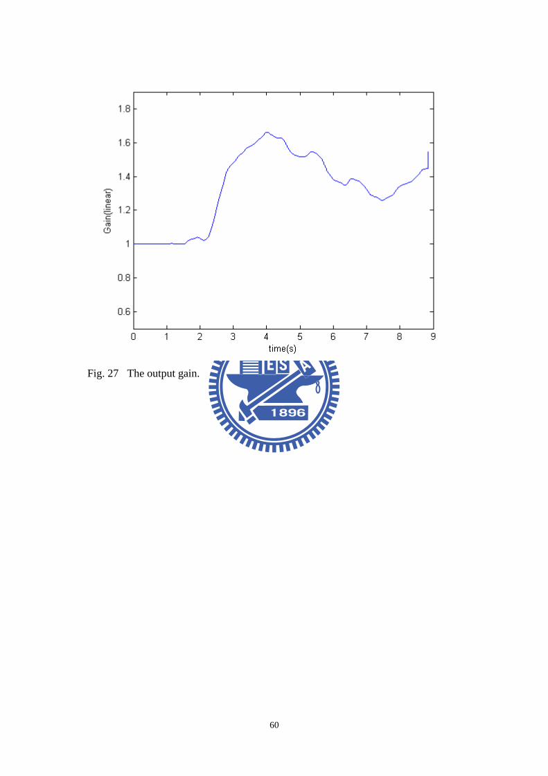
60

Fig. 27 The output gain.

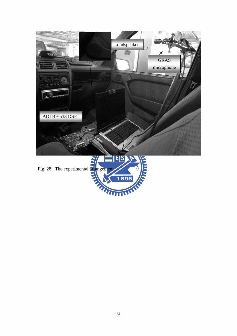
61

Fig. 28 The experimental arrangement.

GRAS

microphone

ADI BF-533 DSP

Loudspeaker

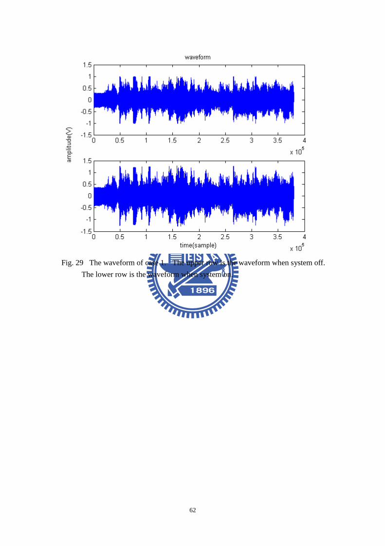
62


The lower row is the waveform when system on.

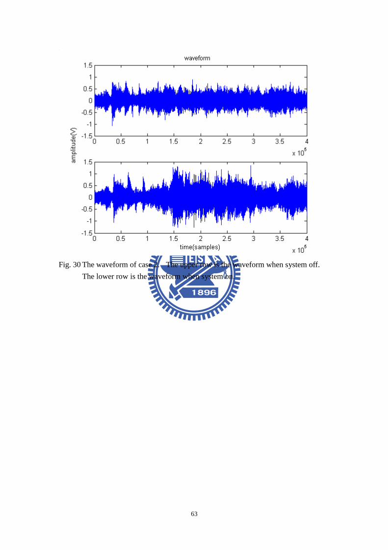
63


The lower row is the waveform when system on.

Documents

國國國 國 立立立立 交交交交 通通通通 大大大大 學學學學 · (VB)以及語音清晰化(VC)的方法，它們分別闡述將頻寬往低頻拓展以 ... (LMS)

國國國國立立立立交交交交通通通通大大大大學學學學 · (VB)以及語音清晰化(VC)的方法，它們分別闡述將頻寬往低頻拓展以 ... (LMS)