On Multi-Class Cost-Sensitive Learning

Zhi-Hua Zhou, Xu-Ying Liu

National Key Laboratory for Novel Software Technology,

Nanjing University, Nanjing 210093, China

{zhouzh, liuxy}@lamda.nju.edu.cn

Abstract

Rescaling is possibly the most popular approach to cost-sensitive learning. This ap-

proach works by rescaling the classes according to their costs, and it can be realized in

different ways, e.g., weighting or sampling the training examples in proportion to their

costs, moving the decision boundary of classifiers faraway from high-cost classes in pro-

portion to costs, etc. This approach is very effective in dealing with two-class problems,

yet some studies showed that it is often not so helpful on multi-class problems. In this

paper, we try to explore why the rescaling approach is often helpless on multi-class prob-

lems. Our analysis discloses that the rescaling approach works well when the costs are

consistent, while directly applying it to multi-class problems with inconsistent costs may

not be a good choice. Based on this recognition, we advocate that before applying the

rescaling approach, the consistency of the costs should be examined at first. If the costs

are consistent, the rescaling approach can be conducted directly; otherwise it is better

to apply rescaling after decomposing the multi-class problem into a series of two-class

problems. An empirical study involving twenty multi-class data sets and seven types of

cost-sensitive learners validates the effectiveness of our proposal. Moreover, we show that

the proposal is also helpful to class-imbalance learning.

Key words: Machine Learning, Data Mining, Cost-Sensitive Learning, Multi-Class

Problems, Rescaling, Class-Imbalance Learning.

1 Introduction

In classical machine learning and data mining settings, the classifiers generally try

to minimize the number of mistakes they will make in classifying new instances.

Such a setting is valid only when the costs of different types of mistakes are equal.

Unfortunately, in many real-world applications the costs of different types of mis-

takes are often unequal. For example, in medical diagnosis, the cost of mistakenly

diagnosing a patient to be healthy may be much larger than that of mistakenly

diagnosing a healthy person as being sick, because the former type of mistake may

result in the loss of a life that can be saved.

Cost-sensitive learning has attracted much attention from the machine learning and

data mining communities. As it has been stated in the Technological Roadmap

of the MLnetII project (European Network of Excellence in Machine Learning)

(Saitta, 2000), the inclusion of costs into learning is one of the most relevant topics

of machine learning research. During the past few years, much effort has been

devoted to cost-sensitive learning. The learning process may involve many kinds

of costs, such as the test cost, teacher cost, intervention cost, etc. (Turney, 2000).

There are many recent studies on test cost (Cebe and Gunduz-Demir, 2007; Chai

et al., 2004; Ling et al., 2004), yet the most studied cost is the misclassification

cost.

Studies on misclassification cost can be categorized into two types further, i.e.,

example-dependent cost (Abe et al., 2004; Brefeld et al., 2003; Lozano and Abe,

2008; Zadrozny and Elkan, 2001; Zadrozny et al., 2002) and class-dependent cost

(Breiman et al., 1984; Domingos, 1999; Drummond and Holte, 2003; Elkan, 2001;

Liu and Zhou, 2006; Maloof, 2003; Margineantu, 2001; Masnadi-Shirazi and Vas-

concelos, 2007; Ting, 2002; Zhang and Zhou, 2008). The former assumes that the

costs are associated with examples, that is, every example has its own misclassifica-

tion cost; the latter assumes that the costs are associated with classes, that is, every

class has its own misclassification cost. It is noteworthy that in most real-world

applications, it is feasible to ask a domain expert to specify the cost of misclassify-

ing a class to another class, yet only in some special tasks it is easy to get the cost

for every training example. In this paper, we will focus on class-dependent costs

and hereafter class-dependent will not be mentioned explicitly for convenience.

The most popular approach to cost-sensitive learning, possibly, is rescaling. This

approach tries to rebalance the classes such that the influences of different classes

on the learning process are in proportion to their costs. A typical process is to

2

assign different weights to training examples of different classes in proportion to

the misclassification costs; then, the weighted examples are given to a learning

algorithm such as C4.5 decision tree to train a model which can be used in future

predictions (Elkan, 2001; Ting, 2002). In addition to weight the training examples,

the rescaling approach can also be realized in many other forms, such as resampling

the training examples (Drummond and Holte, 2003; Elkan, 2001; Maloof, 2003),

moving the decision thresholds (Domingos, 1999; Elkan, 2001), etc.

The rescaling approach has been found effective on two-class problems (Breiman

et al., 1984; Domingos, 1999; Drummond and Holte, 2003; Elkan, 2001; Maloof,

2003; Ting, 2002). However, some studies (Zhou and Liu, 2006b) showed that

it is often not so useful when applied to multi-class problems directly. In fact,

most previous studies on cost-sensitive learning focused on two-class problems,

and although some research involved multi-class data sets (Breiman et al., 1984;

Domingos, 1999; Ting, 2002), only a few studies dedicated to the investigation of

multi-class cost-sensitive learning (Abe et al., 2004; Lozano and Abe, 2008; Zhang

and Zhou, 2008; Zhou and Liu, 2006b) where Abe et al. (2004) and Lozano and

Abe (2008) worked on example-dependent cost while Zhou and Liu (2006b) and

Zhang and Zhou (2008) worked on class-dependent cost.

In this paper, we try to explore why the rescaling approach is often ineffective

on multi-class problems. Our analysis suggests that the rescaling approach could

not work well with inconsistent costs, while many multi-class problems are with

inconsistent costs. Based on this recognition, we advocate that before applying

rescaling, we should examine the consistency of the costs. When the costs are

consistent, we apply rescaling directly; otherwise we apply rescaling after decom-

posing the multi-class problem into a series of two-class problems. To distinguish

the proposed process from the traditional process which executes rescaling without

any sanity checking, we call it Rescalenew. An empirical study involving twenty

multi-class data sets and seven types of cost-sensitive learners validates the effec-

tiveness of the new proposal. Moreover, we show that Rescalenew is also helpful

to class-imbalance learning.

The rest of this paper is organized as follows. Section 2 analyzes why the rescaling

approach is often ineffective on multi-class problems. Section 3 presents Rescalenew.

3

Section 4 reports on our empirical study. Finally, Section 5 concludes.

2 Analysis

Assume that a correct classification costs zero. Let costij (i, j ∈ {1..c}, costii = 0)

denote the cost of misclassifying an example of the i-th class to the j-th class,

where c is the number of classes. It is evident that these costs can be organized

into a cost matrix where the element at the i-th row and the j-th column is costij.

Let ni denote the number of training examples of the i-th class, and n denotes the

total number of training examples. To simplify the discussion, assume there is no

class-imbalance, that is, ni = n/c (i ∈ {1..c}).

Rescaling is a general approach to make any cost-blind learning algorithm cost-

sensitive. The principle is to enable the influence of the higher-cost classes be larger

than that of the lower-cost classes. On two-class problems, the optimal prediction

is the first class if and only if the expected cost of this prediction is no larger than

that of predicting the second class, as shown in Eq. 1 where p = P (class = 1|x).

p× cost11 + (1− p)× cost21 ≤ p× cost12 + (1− p)× cost22 (1)

If the inequality in Eq. 1 becomes equality, predicting either class is optimal. There-

fore, the threshold p∗ for making optimal decision should satisfy Eq. 2.

p∗ × cost11 + (1− p∗)× cost21 = p∗ × cost12 + (1− p∗)× cost22 (2)

Theorem 1 (Elkan, 2001): To make a target probability threshold p∗ correspond

to a given probability threshold p0, the number of the second class examples in the

training set should be multiplied by p∗1−p∗

1−p0

p0.

When the classifier is not biased to any class, the threshold p0 is 0.5. Considering

Eq. 2, Theorem 1 tells that the second class should be rescaled against the first

class according to p∗(1−p∗) = cost21

cost12(remind that cost11 = cost22 = 0), which implies

that the influence of the first class should be cost12cost21

times of that of the second class.

Generally speaking, the optimal rescaling ratio of the i-th class against the j-th

class can be defined as Eq. 3, which indicates that the classes should be rescaled

4

in the way that the influence of the i-th class is τopt(i, j) times of that of the j-th

class. For example, if the weight assigned to the training examples of the j-th class

after rescaling (via weighting the training examples) is wj, then that of the i-th

class will be wi = τopt(i, j)× wj (wi > 0).

τopt(i, j) =costijcostji

(3)

In the traditional rescaling approach (Breiman et al., 1984; Domingos, 1999; Ting,

2002), a quantity costi is derived according to Eq. 4 at first.

costi =∑c

j=1costij (4)

Then, a weight wi is assigned to the i-th class after rescaling (via weighting the

training examples), which is computed according to Eq. 5.

wi =(n× costi)∑c

k=1 (nk × costk)(5)

Remind the assumption ni = n/c, Eq. 5 becomes:

wi =(c× costi)∑c

k=1 costk(6)

So, it is evident that in the traditional rescaling approach, the rescaling ratio of

the i-th class against the j-th class is:

τold(i, j) =wi

wj

=(c× costi) /

∑ck=1 costk

(c× costj) /∑c

k=1 costk=

costicostj

(7)

When c = 2,

τold(i, j) =costicostj

=

∑2k=1 costik∑2k=1 costjk

=cost11 + cost12cost21 + cost22

=cost12cost21

=costijcostji

= τopt(i, j)

This explains that why the traditional rescaling approach can be effective in deal-

ing with the unequal misclassification costs on two-class problems, as shown by

previous research (Breiman et al., 1984; Domingos, 1999; Ting, 2002).

5

Unfortunately, when c > 2, τold(i, j) becomes Eq. 8, which is usually unequal to

τopt(i, j). This explains that why the traditional rescaling approach is often inef-

fective in dealing with the unequal misclassification costs on multi-class problems.

τold(i, j) =costicostj

=

∑ck=1 costik∑ck=1 costjk

(8)

3 Rescalenew

Suppose each class can be assigned with a weight wi (wi > 0) after rescaling (via

weighting the training examples). In order to appropriately rescale all the classes

simultaneously, according to the analysis presented in the previous section, it is

desired that the weights satisfy wi

wj= τopt(i, j) (i, j ∈ {1..c}), which implies the

following (c2) number of constraints:

w1

w2

=cost12

cost21

,w1

w3

=cost13cost31

, · · · , w1

wc

=cost1c

costc1

w2

w3

=cost23cost32

, · · · , w2

wc

=cost2c

costc2

· · · · · · · · ·

wc−1

wc

=costc−1,c

costc,c−1

These constraints can be transformed into the equations shown in Eq. 9. If non-

trivial solution w = [w1, w2, · · · , wc]T can be solved from Eq. 9 (the solution will

be unique, up to a multiplicative factor), then the classes can be appropriately

rescaled simultaneously, which implies that the multi-class cost-sensitive learning

6

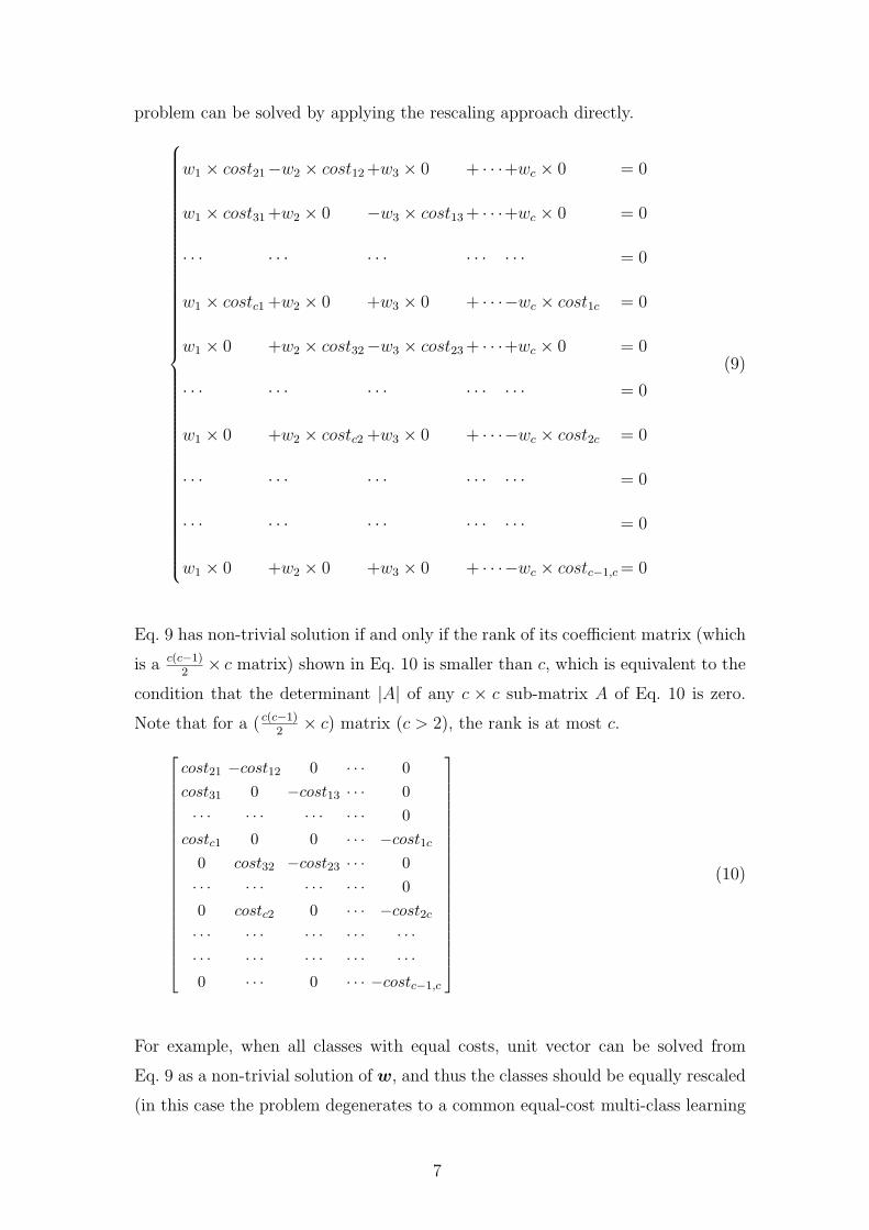
problem can be solved by applying the rescaling approach directly.

w1 × cost21−w2 × cost12 +w3 × 0 + · · ·+wc × 0 = 0

w1 × cost31 +w2 × 0 −w3 × cost13 + · · ·+wc × 0 = 0

· · · · · · · · · · · · · · · = 0

w1 × costc1 +w2 × 0 +w3 × 0 + · · ·−wc × cost1c = 0

w1 × 0 +w2 × cost32−w3 × cost23 + · · ·+wc × 0 = 0

· · · · · · · · · · · · · · · = 0

w1 × 0 +w2 × costc2 +w3 × 0 + · · ·−wc × cost2c = 0

· · · · · · · · · · · · · · · = 0

· · · · · · · · · · · · · · · = 0

w1 × 0 +w2 × 0 +w3 × 0 + · · ·−wc × costc−1,c = 0

(9)

Eq. 9 has non-trivial solution if and only if the rank of its coefficient matrix (which

is a c(c−1)2

× c matrix) shown in Eq. 10 is smaller than c, which is equivalent to the

condition that the determinant |A| of any c × c sub-matrix A of Eq. 10 is zero.

Note that for a ( c(c−1)2

× c) matrix (c > 2), the rank is at most c.

cost21 −cost12 0 · · · 0cost31 0 −cost13 · · · 0· · · · · · · · · · · · 0

costc1 0 0 · · · −cost1c

0 cost32 −cost23 · · · 0· · · · · · · · · · · · 00 costc2 0 · · · −cost2c

· · · · · · · · · · · · · · ·· · · · · · · · · · · · · · ·0 · · · 0 · · · −costc−1,c

(10)

For example, when all classes with equal costs, unit vector can be solved from

Eq. 9 as a non-trivial solution of w, and thus the classes should be equally rescaled

(in this case the problem degenerates to a common equal-cost multi-class learning

7

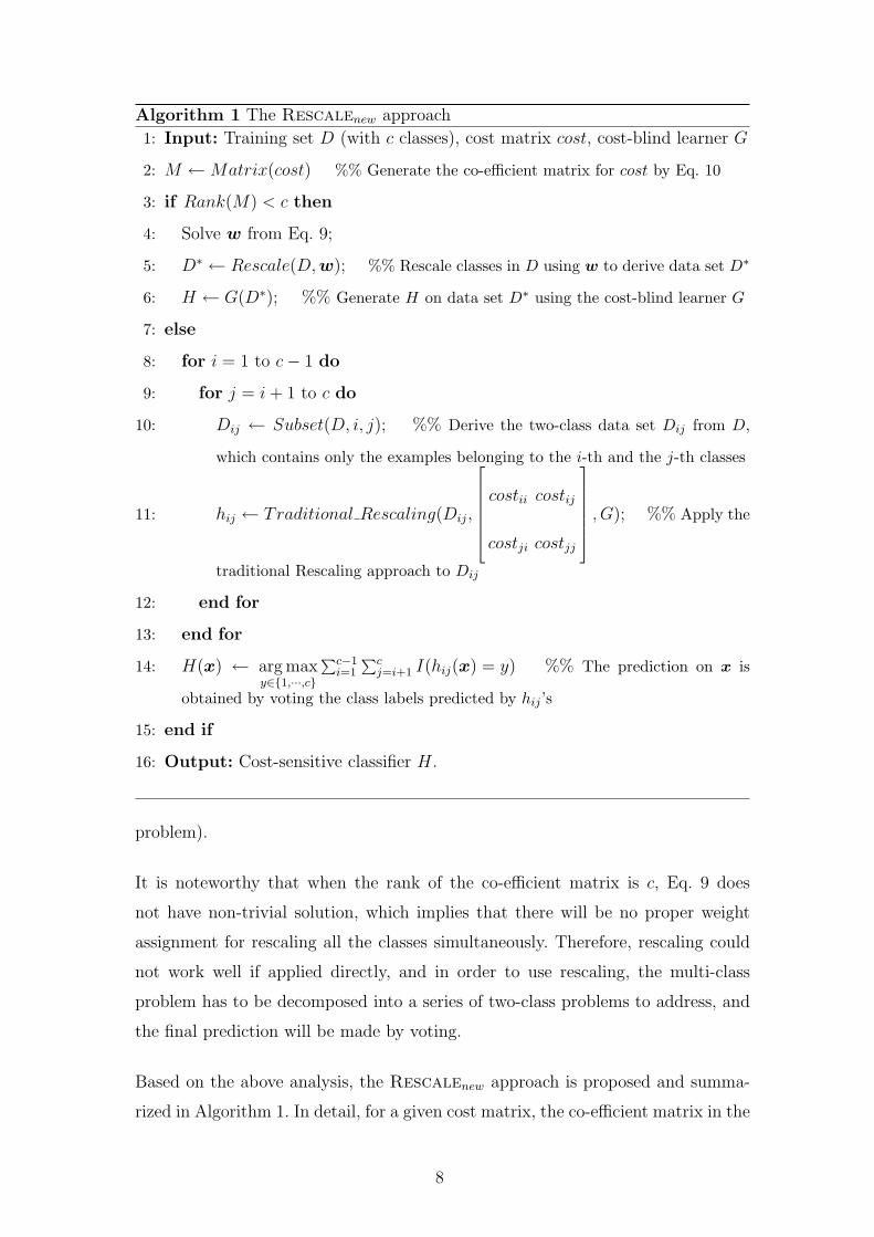
Algorithm 1 The Rescalenew approach

1: Input: Training set D (with c classes), cost matrix cost, cost-blind learner G

2: M ← Matrix(cost) %% Generate the co-efficient matrix for cost by Eq. 10

3: if Rank(M) < c then

4: Solve w from Eq. 9;

5: D∗ ← Rescale(D, w); %% Rescale classes in D using w to derive data set D∗

6: H ← G(D∗); %% Generate H on data set D∗ using the cost-blind learner G

7: else

8: for i = 1 to c− 1 do

9: for j = i + 1 to c do

10: Dij ← Subset(D, i, j); %% Derive the two-class data set Dij from D,

which contains only the examples belonging to the i-th and the j-th classes

11: hij ← Traditional Rescaling(Dij,

costii costij

costji costjj

, G); %% Apply the

traditional Rescaling approach to Dij

12: end for

13: end for

14: H(x) ← arg maxy∈{1,···,c}

∑c−1i=1

∑cj=i+1 I(hij(x) = y) %% The prediction on x is

obtained by voting the class labels predicted by hij ’s

15: end if

16: Output: Cost-sensitive classifier H.

problem).

It is noteworthy that when the rank of the co-efficient matrix is c, Eq. 9 does

not have non-trivial solution, which implies that there will be no proper weight

assignment for rescaling all the classes simultaneously. Therefore, rescaling could

not work well if applied directly, and in order to use rescaling, the multi-class

problem has to be decomposed into a series of two-class problems to address, and

the final prediction will be made by voting.

Based on the above analysis, the Rescalenew approach is proposed and summa-

rized in Algorithm 1. In detail, for a given cost matrix, the co-efficient matrix in the

8

form of Eq. 10 is generated at first. If the rank of the co-efficient matrix is smaller

than c (in this case, the cost matrix is called as a consistent cost matrix), w is

solved from Eq. 9 and used to rescale the classes simultaneously, and the rescaled

data set is then passed to any cost-blind classifier; otherwise (the cost matrix is

called as an inconsistent cost matrix), the multi-class problem is decomposed into

(c2) number of two-class problems, and each two-class data set is rescaled and passed

to any cost-blind classifier, while the final prediction is made by voting the class

labels predicted by the two-class classifiers. Note that there are many alternative

methods for decomposing multi-class problems into a series of two-class problems

(Allwein et al., 2000). Here, we adopt the popular pairwise coupling (that is, every

equation in Eq. 9 corresponds to a two-class problem).

4 Empirical Study

4.1 Methods

In the empirical study we compare Rescalenew (denoted by New) with the tra-

ditional rescaling approach (denoted by Old) (Breiman et al., 1984; Domingos,

1999; Ting, 2002). Here, three ways are used to realize the rescaling process.

The first way is instance-weighting, i.e., weighting the training examples in pro-

portion to costs. Since C4.5 decision tree can deal with weighted examples, we use

it as the cost-blind learner (denoted by Blind-C45). Here we use the J48 imple-

mentation in Weka with default settings (Witten and Frank, 2005). The rescaling

approaches are denoted by Old-IW and New-IW, respectively. Note that in this

way, the Old-IW approach reassembles the C4.5cs method (Ting, 2002).

The second way is resampling. Both over-sampling and under-sampling are ex-

plored. A C4.5 decision tree is trained after sampling process. Thus, the cost-blind

learner is still Blind-C45. By using over-sampling and under-sampling, the tra-

ditional rescaling approaches are denoted by Old-OS and Old-US respectively,

and new rescaling approaches are denoted by New-OS and New-US, respectively.

The third way is threshold-moving. Here the cost-sensitive neural networks devel-

oped by Zhou and Liu (2006b) is used. After training a standard neural network,

9

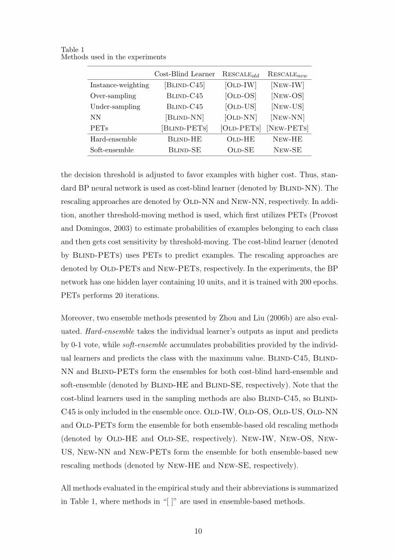
Table 1Methods used in the experiments

Cost-Blind Learner Rescaleold Rescalenew

Instance-weighting [Blind-C45] [Old-IW] [New-IW]Over-sampling Blind-C45 [Old-OS] [New-OS]Under-sampling Blind-C45 [Old-US] [New-US]NN [Blind-NN] [Old-NN] [New-NN]PETs [Blind-PETs] [Old-PETs] [New-PETs]

Hard-ensemble Blind-HE Old-HE New-HE

Soft-ensemble Blind-SE Old-SE New-SE

the decision threshold is adjusted to favor examples with higher cost. Thus, stan-

dard BP neural network is used as cost-blind learner (denoted by Blind-NN). The

rescaling approaches are denoted by Old-NN and New-NN, respectively. In addi-

tion, another threshold-moving method is used, which first utilizes PETs (Provost

and Domingos, 2003) to estimate probabilities of examples belonging to each class

and then gets cost sensitivity by threshold-moving. The cost-blind learner (denoted

by Blind-PETs) uses PETs to predict examples. The rescaling approaches are

denoted by Old-PETs and New-PETs, respectively. In the experiments, the BP

network has one hidden layer containing 10 units, and it is trained with 200 epochs.

PETs performs 20 iterations.

Moreover, two ensemble methods presented by Zhou and Liu (2006b) are also eval-

uated. Hard-ensemble takes the individual learner’s outputs as input and predicts

by 0-1 vote, while soft-ensemble accumulates probabilities provided by the individ-

ual learners and predicts the class with the maximum value. Blind-C45, Blind-

NN and Blind-PETs form the ensembles for both cost-blind hard-ensemble and

soft-ensemble (denoted by Blind-HE and Blind-SE, respectively). Note that the

cost-blind learners used in the sampling methods are also Blind-C45, so Blind-

C45 is only included in the ensemble once. Old-IW, Old-OS, Old-US, Old-NN

and Old-PETs form the ensemble for both ensemble-based old rescaling methods

(denoted by Old-HE and Old-SE, respectively). New-IW, New-OS, New-

US, New-NN and New-PETs form the ensemble for both ensemble-based new

rescaling methods (denoted by New-HE and New-SE, respectively).

All methods evaluated in the empirical study and their abbreviations is summarized

in Table 1, where methods in “[ ]” are used in ensemble-based methods.

10

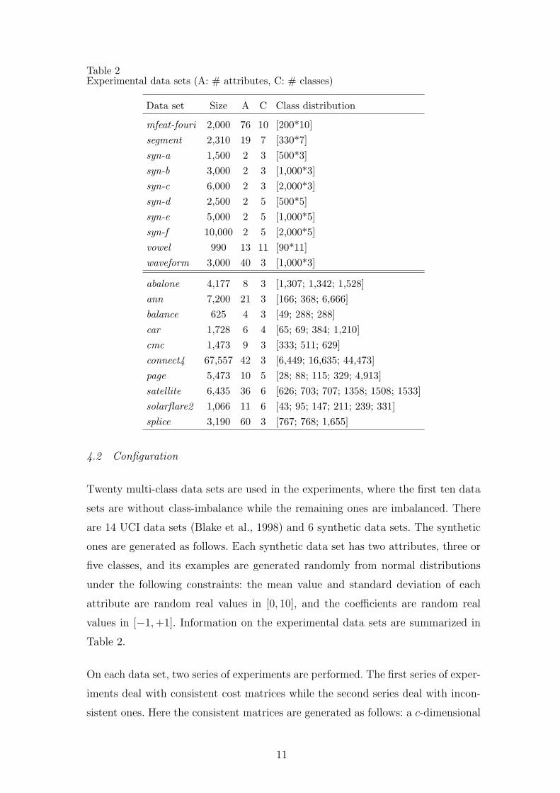
Table 2Experimental data sets (A: # attributes, C: # classes)

Data set Size A C Class distribution

mfeat-fouri 2,000 76 10 [200*10]segment 2,310 19 7 [330*7]syn-a 1,500 2 3 [500*3]syn-b 3,000 2 3 [1,000*3]syn-c 6,000 2 3 [2,000*3]syn-d 2,500 2 5 [500*5]syn-e 5,000 2 5 [1,000*5]syn-f 10,000 2 5 [2,000*5]vowel 990 13 11 [90*11]waveform 3,000 40 3 [1,000*3]

abalone 4,177 8 3 [1,307; 1,342; 1,528]ann 7,200 21 3 [166; 368; 6,666]balance 625 4 3 [49; 288; 288]car 1,728 6 4 [65; 69; 384; 1,210]cmc 1,473 9 3 [333; 511; 629]connect4 67,557 42 3 [6,449; 16,635; 44,473]page 5,473 10 5 [28; 88; 115; 329; 4,913]satellite 6,435 36 6 [626; 703; 707; 1358; 1508; 1533]solarflare2 1,066 11 6 [43; 95; 147; 211; 239; 331]splice 3,190 60 3 [767; 768; 1,655]

4.2 Configuration

Twenty multi-class data sets are used in the experiments, where the first ten data

sets are without class-imbalance while the remaining ones are imbalanced. There

are 14 UCI data sets (Blake et al., 1998) and 6 synthetic data sets. The synthetic

ones are generated as follows. Each synthetic data set has two attributes, three or

five classes, and its examples are generated randomly from normal distributions

under the following constraints: the mean value and standard deviation of each

attribute are random real values in [0, 10], and the coefficients are random real

values in [−1, +1]. Information on the experimental data sets are summarized in

Table 2.

On each data set, two series of experiments are performed. The first series of exper-

iments deal with consistent cost matrices while the second series deal with incon-

sistent ones. Here the consistent matrices are generated as follows: a c-dimensional

11

real value vector is randomly generated and regarded as the root of Eq. 9, then a

real value is randomly generated for costij (i, j ∈ [1, c] and i 6= j) such that costji

can be solved from Eq. 9. All these real values are in [1, 10], costii = 0 and at least

one costij is 1.0. Note that in generating cost matrices for imbalanced data sets, it

is constrained that the cost of misclassifying the smallest class to the largest class

is the biggest while the cost of misclassifying the largest class to the smallest class

is the smallest. This owes to the fact that when the largest class is with the biggest

misclassification cost, classical machine learning approaches are good enough and

therefore this situation is not concerned in the research of cost-sensitive learning

and class-imbalance learning. The inconsistent matrices are generated in a similar

way except that one costji solved from Eq. 9 is replaced by a random value. The

ranks of the co-efficient matrices corresponding to those cost matrices have been

examined to guarantee that they are smaller or not smaller than c, respectively.

In each series of experiments, ten times 10-fold cross validation are performed.

Concretely, 10-fold cross validation is repeated for ten times with randomly gener-

ated cost matrices belonging to the same type (i.e. consistent or inconsistent), and

the average results are recorded.

There are some powerful tools such as Roc and cost curves (Drummond and Holte,

2000) for visually evaluating the performance of two-class cost-sensitive learning

approaches. Unfortunately, they could not be applied to multi-class problems di-

rectly. So, here the misclassification costs are compared.

4.3 Results

The influences of the traditional rescaling approach and the new rescaling ap-

proach on instance-weighting-based cost-sensitive C4.5, over-sampling-based cost-

sensitive C4.5, under-sampling-based cost-sensitive C4.5, threshold-moving-based

cost-sensitive neural network, threshold-moving-based cost-sensitive PETs, hard-

ensemble and soft-ensemble are reported separately.

4.3.1 On Instance-Weighting-Based Cost-Sensitive C4.5

Tables 3 and 4 present the performance of the traditional rescaling approach and

the new rescaling approach on instance-weighting-based cost-sensitive C4.5 on con-

12

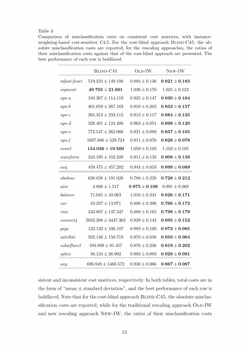
Table 3Comparison of misclassification costs on consistent cost matrices, with instance-weighting-based cost-sensitive C4.5. For the cost-blind approach Blind-C45, the ab-solute misclassification costs are reported; for the rescaling approaches, the ratios oftheir misclassification costs against that of the cost-blind approach are presented. Thebest performance of each row is boldfaced.

Blind-C45 Old-IW New-IW

mfeat-fouri 519.234± 149.108 0.894± 0.136 0.821± 0.183

segment 49.705± 21.601 1.030± 0.170 1.025± 0.123

syn-a 183.307± 114.119 0.925± 0.147 0.830± 0.184

syn-b 401.059± 267.163 0.910± 0.202 0.833± 0.157

syn-c 265.313± 259.115 0.913± 0.117 0.884± 0.135

syn-d 328.491± 124.408 0.963± 0.051 0.898± 0.120

syn-e 772.547± 262.066 0.921± 0.089 0.857± 0.105

syn-f 1697.866± 529.724 0.911± 0.076 0.828± 0.078

vowel 134.036± 19.500 1.059± 0.102 1.102± 0.105

waveform 243.195± 102.328 0.911± 0.133 0.908± 0.139

avg. 459.475± 457.202 0.944± 0.053 0.899± 0.089

abalone 638.828± 191.028 0.788± 0.220 0.728± 0.212

ann 4.806± 1.517 0.975± 0.106 0.991± 0.069

balance 71.045± 43.063 1.016± 0.231 0.826± 0.171

car 43.287± 13.971 0.888± 0.206 0.766± 0.172

cmc 243.007± 137.347 0.888± 0.165 0.798± 0.179

connect4 5032.208± 3447.362 0.928± 0.143 0.895± 0.152

page 122.133± 106.107 0.983± 0.100 0.972± 0.085

satellite 502.146± 150.719 0.970± 0.056 0.950± 0.064

solarflare2 194.899± 91.457 0.876± 0.236 0.819± 0.202

splice 56.124± 26.992 0.983± 0.093 0.929± 0.091

avg. 690.848± 1460.572 0.930± 0.066 0.867± 0.087

sistent and inconsistent cost matrices, respectively. In both tables, total costs are in

the form of “mean ± standard deviation”, and the best performance of each row is

boldfaced. Note that for the cost-blind approach Blind-C45, the absolute misclas-

sification costs are reported; while for the traditional rescaling approach Old-IW

and new rescaling approach New-IW, the ratios of their misclassification costs

13

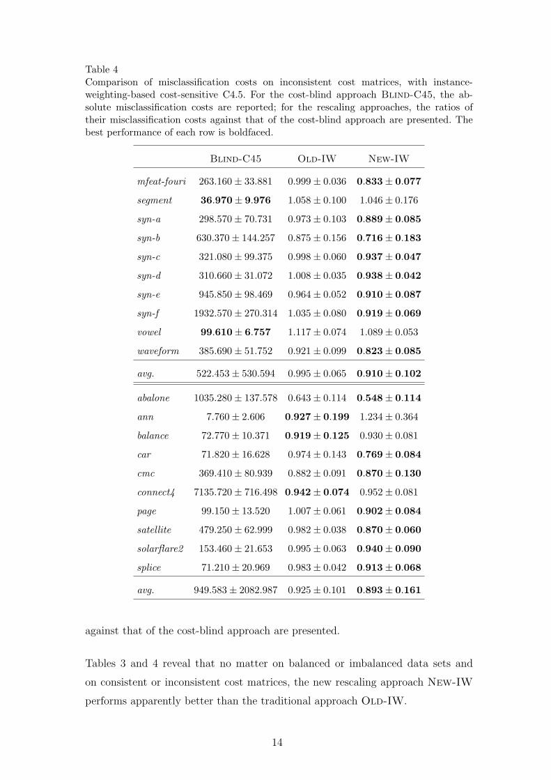
Table 4Comparison of misclassification costs on inconsistent cost matrices, with instance-weighting-based cost-sensitive C4.5. For the cost-blind approach Blind-C45, the ab-solute misclassification costs are reported; for the rescaling approaches, the ratios oftheir misclassification costs against that of the cost-blind approach are presented. Thebest performance of each row is boldfaced.

Blind-C45 Old-IW New-IW

mfeat-fouri 263.160± 33.881 0.999± 0.036 0.833± 0.077

segment 36.970± 9.976 1.058± 0.100 1.046± 0.176

syn-a 298.570± 70.731 0.973± 0.103 0.889± 0.085

syn-b 630.370± 144.257 0.875± 0.156 0.716± 0.183

syn-c 321.080± 99.375 0.998± 0.060 0.937± 0.047

syn-d 310.660± 31.072 1.008± 0.035 0.938± 0.042

syn-e 945.850± 98.469 0.964± 0.052 0.910± 0.087

syn-f 1932.570± 270.314 1.035± 0.080 0.919± 0.069

vowel 99.610± 6.757 1.117± 0.074 1.089± 0.053

waveform 385.690± 51.752 0.921± 0.099 0.823± 0.085

avg. 522.453± 530.594 0.995± 0.065 0.910± 0.102

abalone 1035.280± 137.578 0.643± 0.114 0.548± 0.114

ann 7.760± 2.606 0.927± 0.199 1.234± 0.364

balance 72.770± 10.371 0.919± 0.125 0.930± 0.081

car 71.820± 16.628 0.974± 0.143 0.769± 0.084

cmc 369.410± 80.939 0.882± 0.091 0.870± 0.130

connect4 7135.720± 716.498 0.942± 0.074 0.952± 0.081

page 99.150± 13.520 1.007± 0.061 0.902± 0.084

satellite 479.250± 62.999 0.982± 0.038 0.870± 0.060

solarflare2 153.460± 21.653 0.995± 0.063 0.940± 0.090

splice 71.210± 20.969 0.983± 0.042 0.913± 0.068

avg. 949.583± 2082.987 0.925± 0.101 0.893± 0.161

against that of the cost-blind approach are presented.

Tables 3 and 4 reveal that no matter on balanced or imbalanced data sets and

on consistent or inconsistent cost matrices, the new rescaling approach New-IW

performs apparently better than the traditional approach Old-IW.

14

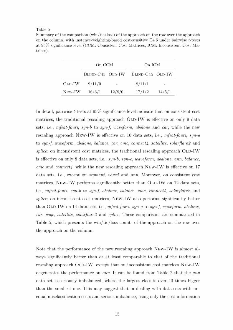
Table 5Summary of the comparison (win/tie/loss) of the approach on the row over the approachon the column, with instance-weighting-based cost-sensitive C4.5 under pairwise t-testsat 95% significance level (CCM: Consistent Cost Matrices, ICM: Inconsistent Cost Ma-trices).

On CCM On ICM

Blind-C45 Old-IW Blind-C45 Old-IW

Old-IW 9/11/0 - 8/11/1 -

New-IW 16/3/1 12/8/0 17/1/2 14/5/1

In detail, pairwise t-tests at 95% significance level indicate that on consistent cost

matrices, the traditional rescaling approach Old-IW is effective on only 9 data

sets, i.e., mfeat-fouri, syn-b to syn-f, waveform, abalone and car, while the new

rescaling approach New-IW is effective on 16 data sets, i.e., mfeat-fouri, syn-a

to syn-f, waveform, abalone, balance, car, cmc, connect4, satellite, solarflare2 and

splice; on inconsistent cost matrices, the traditional rescaling approach Old-IW

is effective on only 8 data sets, i.e., syn-b, syn-e, waveform, abalone, ann, balance,

cmc and connect4, while the new rescaling approach New-IW is effective on 17

data sets, i.e., except on segment, vowel and ann. Moreover, on consistent cost

matrices, New-IW performs significantly better than Old-IW on 12 data sets,

i.e., mfeat-fouri, syn-b to syn-f, abalone, balance, cmc, connect4, solarflare2 and

splice; on inconsistent cost matrices, New-IW also performs significantly better

than Old-IW on 14 data sets, i.e., mfeat-fouri, syn-a to syn-f, waveform, abalone,

car, page, satellite, solarflare2 and splice. These comparisons are summarized in

Table 5, which presents the win/tie/loss counts of the approach on the row over

the approach on the column.

Note that the performance of the new rescaling approach New-IW is almost al-

ways significantly better than or at least comparable to that of the traditional

rescaling approach Old-IW, except that on inconsistent cost matrices New-IW

degenerates the performance on ann. It can be found from Table 2 that the ann

data set is seriously imbalanced, where the largest class is over 40 times bigger

than the smallest one. This may suggest that in dealing with data sets with un-

equal misclassification costs and serious imbalance, using only the cost information

15

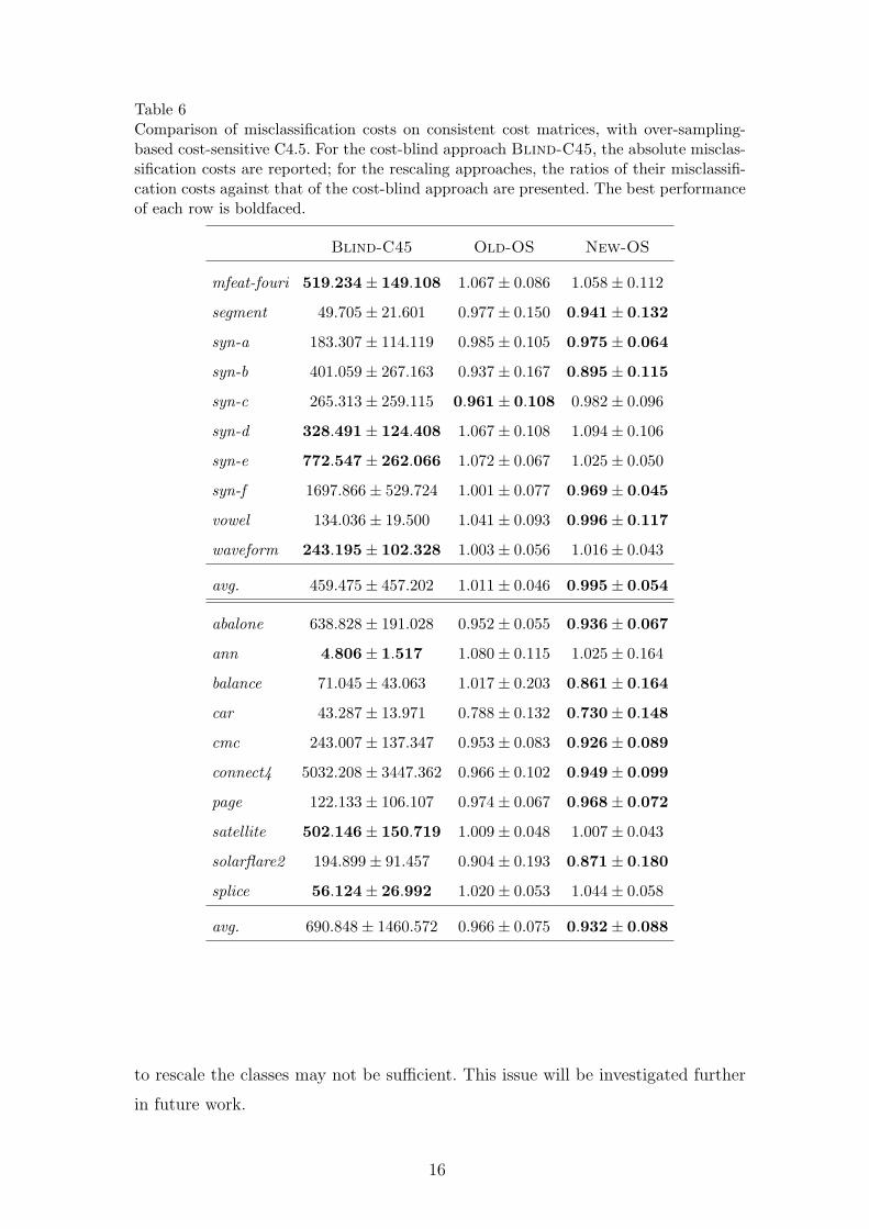
Table 6Comparison of misclassification costs on consistent cost matrices, with over-sampling-based cost-sensitive C4.5. For the cost-blind approach Blind-C45, the absolute misclas-sification costs are reported; for the rescaling approaches, the ratios of their misclassifi-cation costs against that of the cost-blind approach are presented. The best performanceof each row is boldfaced.

Blind-C45 Old-OS New-OS

mfeat-fouri 519.234± 149.108 1.067± 0.086 1.058± 0.112

segment 49.705± 21.601 0.977± 0.150 0.941± 0.132

syn-a 183.307± 114.119 0.985± 0.105 0.975± 0.064

syn-b 401.059± 267.163 0.937± 0.167 0.895± 0.115

syn-c 265.313± 259.115 0.961± 0.108 0.982± 0.096

syn-d 328.491± 124.408 1.067± 0.108 1.094± 0.106

syn-e 772.547± 262.066 1.072± 0.067 1.025± 0.050

syn-f 1697.866± 529.724 1.001± 0.077 0.969± 0.045

vowel 134.036± 19.500 1.041± 0.093 0.996± 0.117

waveform 243.195± 102.328 1.003± 0.056 1.016± 0.043

avg. 459.475± 457.202 1.011± 0.046 0.995± 0.054

abalone 638.828± 191.028 0.952± 0.055 0.936± 0.067

ann 4.806± 1.517 1.080± 0.115 1.025± 0.164

balance 71.045± 43.063 1.017± 0.203 0.861± 0.164

car 43.287± 13.971 0.788± 0.132 0.730± 0.148

cmc 243.007± 137.347 0.953± 0.083 0.926± 0.089

connect4 5032.208± 3447.362 0.966± 0.102 0.949± 0.099

page 122.133± 106.107 0.974± 0.067 0.968± 0.072

satellite 502.146± 150.719 1.009± 0.048 1.007± 0.043

solarflare2 194.899± 91.457 0.904± 0.193 0.871± 0.180

splice 56.124± 26.992 1.020± 0.053 1.044± 0.058

avg. 690.848± 1460.572 0.966± 0.075 0.932± 0.088

to rescale the classes may not be sufficient. This issue will be investigated further

in future work.

16

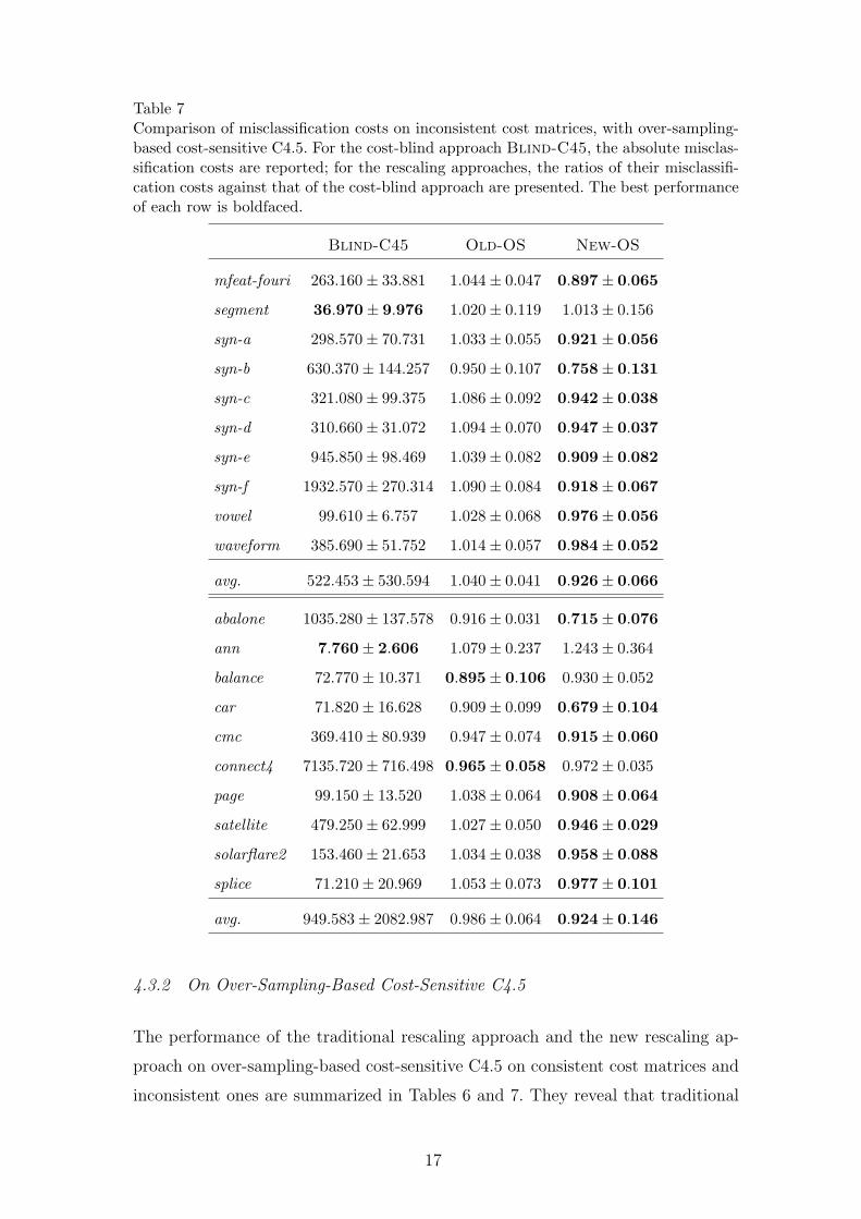
Table 7Comparison of misclassification costs on inconsistent cost matrices, with over-sampling-based cost-sensitive C4.5. For the cost-blind approach Blind-C45, the absolute misclas-sification costs are reported; for the rescaling approaches, the ratios of their misclassifi-cation costs against that of the cost-blind approach are presented. The best performanceof each row is boldfaced.

Blind-C45 Old-OS New-OS

mfeat-fouri 263.160± 33.881 1.044± 0.047 0.897± 0.065

segment 36.970± 9.976 1.020± 0.119 1.013± 0.156

syn-a 298.570± 70.731 1.033± 0.055 0.921± 0.056

syn-b 630.370± 144.257 0.950± 0.107 0.758± 0.131

syn-c 321.080± 99.375 1.086± 0.092 0.942± 0.038

syn-d 310.660± 31.072 1.094± 0.070 0.947± 0.037

syn-e 945.850± 98.469 1.039± 0.082 0.909± 0.082

syn-f 1932.570± 270.314 1.090± 0.084 0.918± 0.067

vowel 99.610± 6.757 1.028± 0.068 0.976± 0.056

waveform 385.690± 51.752 1.014± 0.057 0.984± 0.052

avg. 522.453± 530.594 1.040± 0.041 0.926± 0.066

abalone 1035.280± 137.578 0.916± 0.031 0.715± 0.076

ann 7.760± 2.606 1.079± 0.237 1.243± 0.364

balance 72.770± 10.371 0.895± 0.106 0.930± 0.052

car 71.820± 16.628 0.909± 0.099 0.679± 0.104

cmc 369.410± 80.939 0.947± 0.074 0.915± 0.060

connect4 7135.720± 716.498 0.965± 0.058 0.972± 0.035

page 99.150± 13.520 1.038± 0.064 0.908± 0.064

satellite 479.250± 62.999 1.027± 0.050 0.946± 0.029

solarflare2 153.460± 21.653 1.034± 0.038 0.958± 0.088

splice 71.210± 20.969 1.053± 0.073 0.977± 0.101

avg. 949.583± 2082.987 0.986± 0.064 0.924± 0.146

4.3.2 On Over-Sampling-Based Cost-Sensitive C4.5

The performance of the traditional rescaling approach and the new rescaling ap-

proach on over-sampling-based cost-sensitive C4.5 on consistent cost matrices and

inconsistent ones are summarized in Tables 6 and 7. They reveal that traditional

17

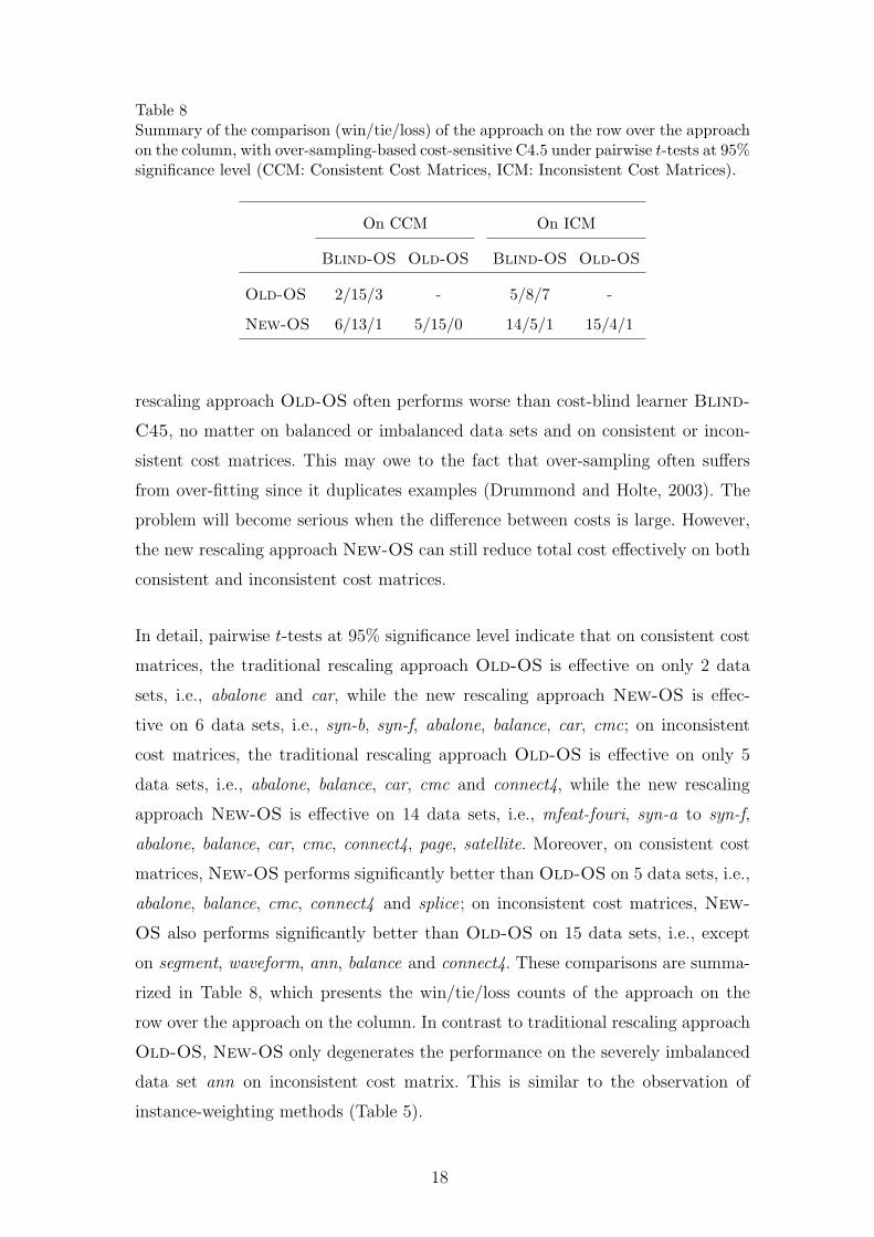
Table 8Summary of the comparison (win/tie/loss) of the approach on the row over the approachon the column, with over-sampling-based cost-sensitive C4.5 under pairwise t-tests at 95%significance level (CCM: Consistent Cost Matrices, ICM: Inconsistent Cost Matrices).

On CCM On ICM

Blind-OS Old-OS Blind-OS Old-OS

Old-OS 2/15/3 - 5/8/7 -

New-OS 6/13/1 5/15/0 14/5/1 15/4/1

rescaling approach Old-OS often performs worse than cost-blind learner Blind-

C45, no matter on balanced or imbalanced data sets and on consistent or incon-

sistent cost matrices. This may owe to the fact that over-sampling often suffers

from over-fitting since it duplicates examples (Drummond and Holte, 2003). The

problem will become serious when the difference between costs is large. However,

the new rescaling approach New-OS can still reduce total cost effectively on both

consistent and inconsistent cost matrices.

In detail, pairwise t-tests at 95% significance level indicate that on consistent cost

matrices, the traditional rescaling approach Old-OS is effective on only 2 data

sets, i.e., abalone and car, while the new rescaling approach New-OS is effec-

tive on 6 data sets, i.e., syn-b, syn-f, abalone, balance, car, cmc; on inconsistent

cost matrices, the traditional rescaling approach Old-OS is effective on only 5

data sets, i.e., abalone, balance, car, cmc and connect4, while the new rescaling

approach New-OS is effective on 14 data sets, i.e., mfeat-fouri, syn-a to syn-f,

abalone, balance, car, cmc, connect4, page, satellite. Moreover, on consistent cost

matrices, New-OS performs significantly better than Old-OS on 5 data sets, i.e.,

abalone, balance, cmc, connect4 and splice; on inconsistent cost matrices, New-

OS also performs significantly better than Old-OS on 15 data sets, i.e., except

on segment, waveform, ann, balance and connect4. These comparisons are summa-

rized in Table 8, which presents the win/tie/loss counts of the approach on the

row over the approach on the column. In contrast to traditional rescaling approach

Old-OS, New-OS only degenerates the performance on the severely imbalanced

data set ann on inconsistent cost matrix. This is similar to the observation of

instance-weighting methods (Table 5).

18

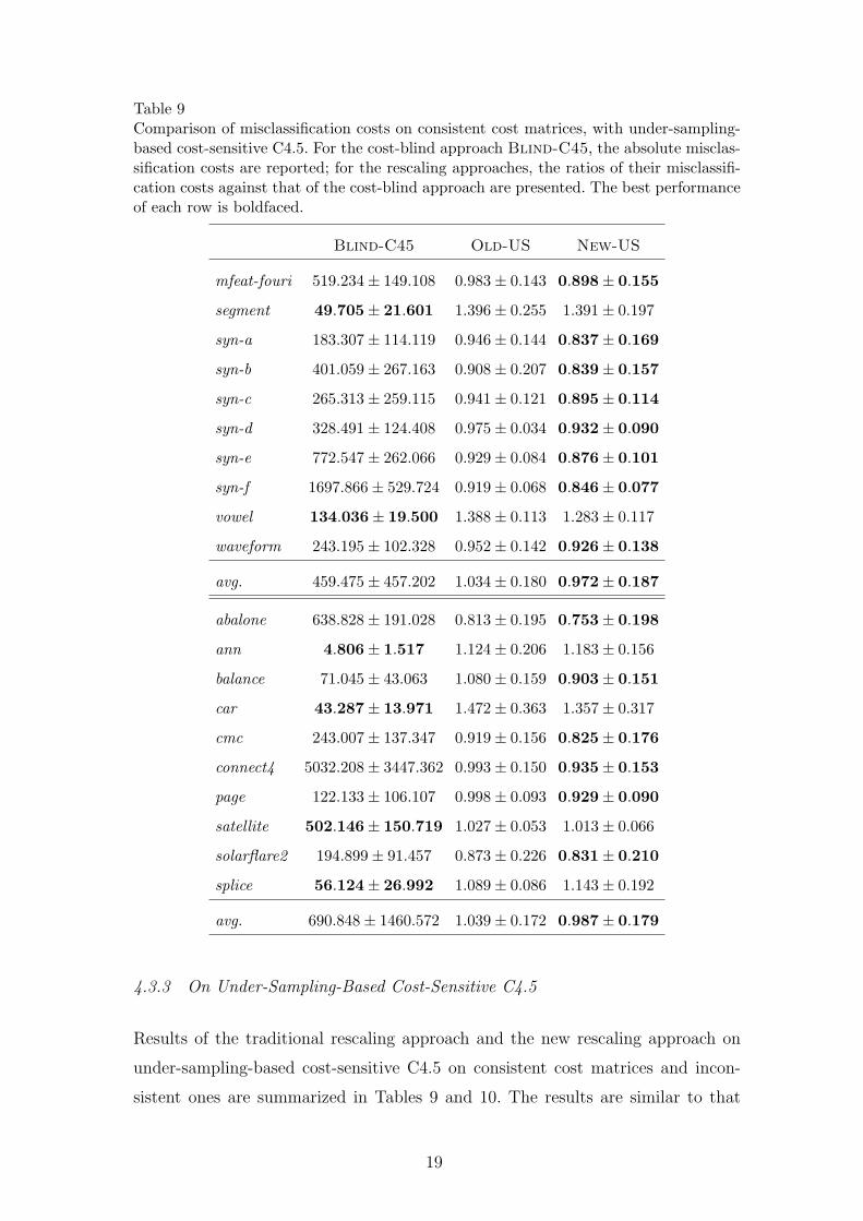
Table 9Comparison of misclassification costs on consistent cost matrices, with under-sampling-based cost-sensitive C4.5. For the cost-blind approach Blind-C45, the absolute misclas-sification costs are reported; for the rescaling approaches, the ratios of their misclassifi-cation costs against that of the cost-blind approach are presented. The best performanceof each row is boldfaced.

Blind-C45 Old-US New-US

mfeat-fouri 519.234± 149.108 0.983± 0.143 0.898± 0.155

segment 49.705± 21.601 1.396± 0.255 1.391± 0.197

syn-a 183.307± 114.119 0.946± 0.144 0.837± 0.169

syn-b 401.059± 267.163 0.908± 0.207 0.839± 0.157

syn-c 265.313± 259.115 0.941± 0.121 0.895± 0.114

syn-d 328.491± 124.408 0.975± 0.034 0.932± 0.090

syn-e 772.547± 262.066 0.929± 0.084 0.876± 0.101

syn-f 1697.866± 529.724 0.919± 0.068 0.846± 0.077

vowel 134.036± 19.500 1.388± 0.113 1.283± 0.117

waveform 243.195± 102.328 0.952± 0.142 0.926± 0.138

avg. 459.475± 457.202 1.034± 0.180 0.972± 0.187

abalone 638.828± 191.028 0.813± 0.195 0.753± 0.198

ann 4.806± 1.517 1.124± 0.206 1.183± 0.156

balance 71.045± 43.063 1.080± 0.159 0.903± 0.151

car 43.287± 13.971 1.472± 0.363 1.357± 0.317

cmc 243.007± 137.347 0.919± 0.156 0.825± 0.176

connect4 5032.208± 3447.362 0.993± 0.150 0.935± 0.153

page 122.133± 106.107 0.998± 0.093 0.929± 0.090

satellite 502.146± 150.719 1.027± 0.053 1.013± 0.066

solarflare2 194.899± 91.457 0.873± 0.226 0.831± 0.210

splice 56.124± 26.992 1.089± 0.086 1.143± 0.192

avg. 690.848± 1460.572 1.039± 0.172 0.987± 0.179

4.3.3 On Under-Sampling-Based Cost-Sensitive C4.5

Results of the traditional rescaling approach and the new rescaling approach on

under-sampling-based cost-sensitive C4.5 on consistent cost matrices and incon-

sistent ones are summarized in Tables 9 and 10. The results are similar to that

19

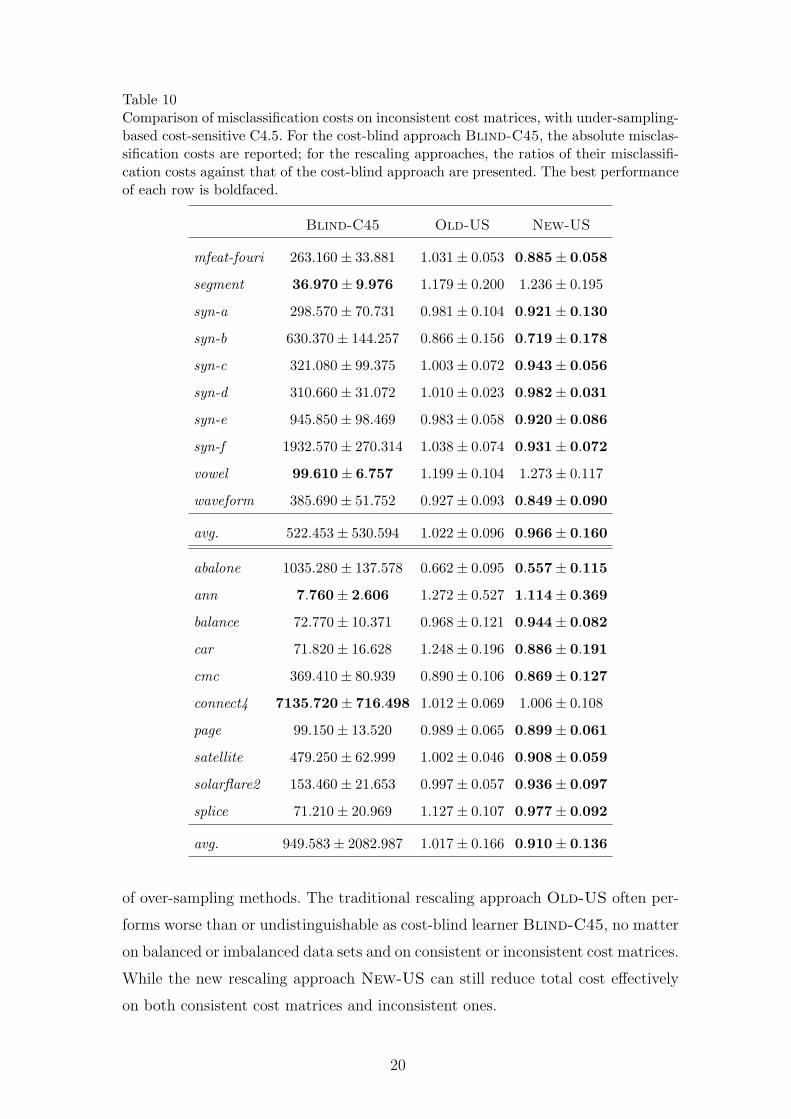
Table 10Comparison of misclassification costs on inconsistent cost matrices, with under-sampling-based cost-sensitive C4.5. For the cost-blind approach Blind-C45, the absolute misclas-sification costs are reported; for the rescaling approaches, the ratios of their misclassifi-cation costs against that of the cost-blind approach are presented. The best performanceof each row is boldfaced.

Blind-C45 Old-US New-US

mfeat-fouri 263.160± 33.881 1.031± 0.053 0.885± 0.058

segment 36.970± 9.976 1.179± 0.200 1.236± 0.195

syn-a 298.570± 70.731 0.981± 0.104 0.921± 0.130

syn-b 630.370± 144.257 0.866± 0.156 0.719± 0.178

syn-c 321.080± 99.375 1.003± 0.072 0.943± 0.056

syn-d 310.660± 31.072 1.010± 0.023 0.982± 0.031

syn-e 945.850± 98.469 0.983± 0.058 0.920± 0.086

syn-f 1932.570± 270.314 1.038± 0.074 0.931± 0.072

vowel 99.610± 6.757 1.199± 0.104 1.273± 0.117

waveform 385.690± 51.752 0.927± 0.093 0.849± 0.090

avg. 522.453± 530.594 1.022± 0.096 0.966± 0.160

abalone 1035.280± 137.578 0.662± 0.095 0.557± 0.115

ann 7.760± 2.606 1.272± 0.527 1.114± 0.369

balance 72.770± 10.371 0.968± 0.121 0.944± 0.082

car 71.820± 16.628 1.248± 0.196 0.886± 0.191

cmc 369.410± 80.939 0.890± 0.106 0.869± 0.127

connect4 7135.720± 716.498 1.012± 0.069 1.006± 0.108

page 99.150± 13.520 0.989± 0.065 0.899± 0.061

satellite 479.250± 62.999 1.002± 0.046 0.908± 0.059

solarflare2 153.460± 21.653 0.997± 0.057 0.936± 0.097

splice 71.210± 20.969 1.127± 0.107 0.977± 0.092

avg. 949.583± 2082.987 1.017± 0.166 0.910± 0.136

of over-sampling methods. The traditional rescaling approach Old-US often per-

forms worse than or undistinguishable as cost-blind learner Blind-C45, no matter

on balanced or imbalanced data sets and on consistent or inconsistent cost matrices.

While the new rescaling approach New-US can still reduce total cost effectively

on both consistent cost matrices and inconsistent ones.

20

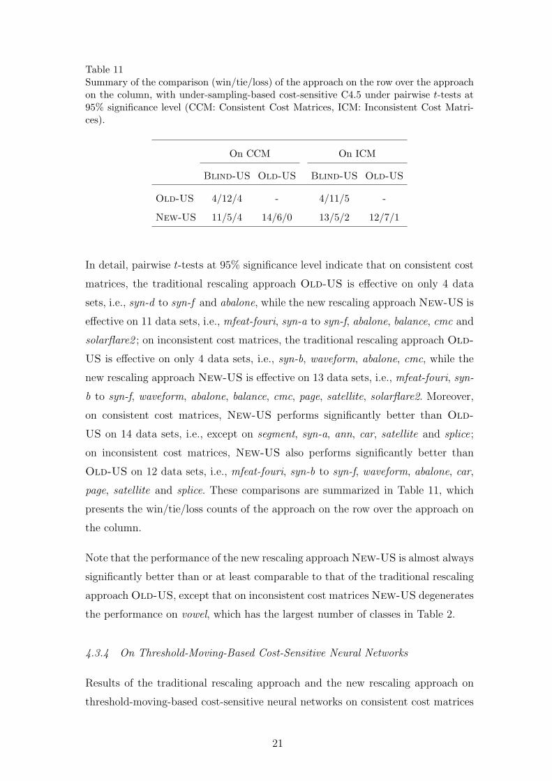
Table 11Summary of the comparison (win/tie/loss) of the approach on the row over the approachon the column, with under-sampling-based cost-sensitive C4.5 under pairwise t-tests at95% significance level (CCM: Consistent Cost Matrices, ICM: Inconsistent Cost Matri-ces).

On CCM On ICM

Blind-US Old-US Blind-US Old-US

Old-US 4/12/4 - 4/11/5 -

New-US 11/5/4 14/6/0 13/5/2 12/7/1

In detail, pairwise t-tests at 95% significance level indicate that on consistent cost

matrices, the traditional rescaling approach Old-US is effective on only 4 data

sets, i.e., syn-d to syn-f and abalone, while the new rescaling approach New-US is

effective on 11 data sets, i.e., mfeat-fouri, syn-a to syn-f, abalone, balance, cmc and

solarflare2 ; on inconsistent cost matrices, the traditional rescaling approach Old-

US is effective on only 4 data sets, i.e., syn-b, waveform, abalone, cmc, while the

new rescaling approach New-US is effective on 13 data sets, i.e., mfeat-fouri, syn-

b to syn-f, waveform, abalone, balance, cmc, page, satellite, solarflare2. Moreover,

on consistent cost matrices, New-US performs significantly better than Old-

US on 14 data sets, i.e., except on segment, syn-a, ann, car, satellite and splice;

on inconsistent cost matrices, New-US also performs significantly better than

Old-US on 12 data sets, i.e., mfeat-fouri, syn-b to syn-f, waveform, abalone, car,

page, satellite and splice. These comparisons are summarized in Table 11, which

presents the win/tie/loss counts of the approach on the row over the approach on

the column.

Note that the performance of the new rescaling approach New-US is almost always

significantly better than or at least comparable to that of the traditional rescaling

approach Old-US, except that on inconsistent cost matrices New-US degenerates

the performance on vowel, which has the largest number of classes in Table 2.

4.3.4 On Threshold-Moving-Based Cost-Sensitive Neural Networks

Results of the traditional rescaling approach and the new rescaling approach on

threshold-moving-based cost-sensitive neural networks on consistent cost matrices

21

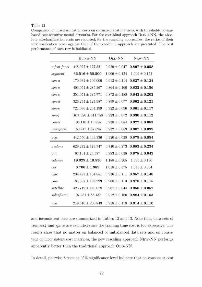
Table 12Comparison of misclassification costs on consistent cost matrices, with threshold-moving-based cost-sensitive neural networks. For the cost-blind approach Blind-NN, the abso-lute misclassification costs are reported; for the rescaling approaches, the ratios of theirmisclassification costs against that of the cost-blind approach are presented. The bestperformance of each row is boldfaced.

Blind-NN Old-NN New-NN

mfeat-fouri 448.927± 127.321 0.929± 0.047 0.897± 0.058

segment 66.516± 55.500 1.009± 0.124 1.009± 0.152

syn-a 170.932± 106.006 0.913± 0.114 0.827± 0.134

syn-b 403.054± 285.367 0.864± 0.160 0.832± 0.156

syn-c 351.051± 385.771 0.872± 0.188 0.842± 0.202

syn-d 326.244± 124.987 0.899± 0.077 0.862± 0.121

syn-e 721.096± 234.199 0.922± 0.096 0.861± 0.117

syn-f 1671.320± 611.758 0.923± 0.072 0.830± 0.112

vowel 106.110± 13.855 0.938± 0.084 0.922± 0.083

waveform 160.247± 67.895 0.932± 0.089 0.907± 0.099

avg. 442.550± 449.336 0.920± 0.038 0.879± 0.054

abalone 629.272± 173.747 0.740± 0.273 0.683± 0.234

ann 63.101± 24.587 0.993± 0.038 0.978± 0.042

balance 19.029± 10.530 1.188± 0.305 1.035± 0.196

car 3.706± 1.989 1.018± 0.375 1.045± 0.364

cmc 234.423± 134.851 0.936± 0.111 0.857± 0.146

page 185.597± 152.299 0.908± 0.113 0.876± 0.115

satellite 423.719± 140.078 0.967± 0.044 0.956± 0.057

solarflare2 197.231± 88.437 0.912± 0.160 0.884± 0.163

avg. 219.510± 200.843 0.958± 0.118 0.914± 0.110

and inconsistent ones are summarized in Tables 12 and 13. Note that, data sets of

connect4 and splice are excluded since the training time cost is too expensive. The

results show that no matter on balanced or imbalanced data sets and on consis-

tent or inconsistent cost matrices, the new rescaling approach New-NN performs

apparently better than the traditional approach Old-NN.

In detail, pairwise t-tests at 95% significance level indicate that on consistent cost

22

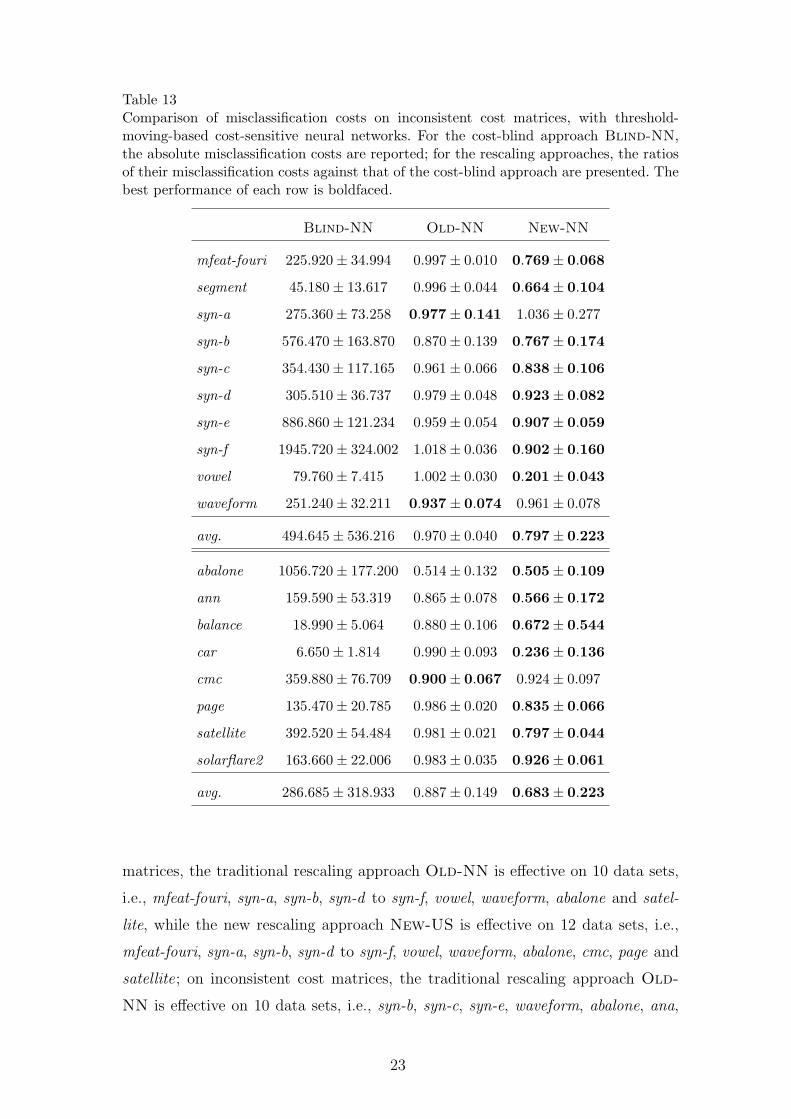
Table 13Comparison of misclassification costs on inconsistent cost matrices, with threshold-moving-based cost-sensitive neural networks. For the cost-blind approach Blind-NN,the absolute misclassification costs are reported; for the rescaling approaches, the ratiosof their misclassification costs against that of the cost-blind approach are presented. Thebest performance of each row is boldfaced.

Blind-NN Old-NN New-NN

mfeat-fouri 225.920± 34.994 0.997± 0.010 0.769± 0.068

segment 45.180± 13.617 0.996± 0.044 0.664± 0.104

syn-a 275.360± 73.258 0.977± 0.141 1.036± 0.277

syn-b 576.470± 163.870 0.870± 0.139 0.767± 0.174

syn-c 354.430± 117.165 0.961± 0.066 0.838± 0.106

syn-d 305.510± 36.737 0.979± 0.048 0.923± 0.082

syn-e 886.860± 121.234 0.959± 0.054 0.907± 0.059

syn-f 1945.720± 324.002 1.018± 0.036 0.902± 0.160

vowel 79.760± 7.415 1.002± 0.030 0.201± 0.043

waveform 251.240± 32.211 0.937± 0.074 0.961± 0.078

avg. 494.645± 536.216 0.970± 0.040 0.797± 0.223

abalone 1056.720± 177.200 0.514± 0.132 0.505± 0.109

ann 159.590± 53.319 0.865± 0.078 0.566± 0.172

balance 18.990± 5.064 0.880± 0.106 0.672± 0.544

car 6.650± 1.814 0.990± 0.093 0.236± 0.136

cmc 359.880± 76.709 0.900± 0.067 0.924± 0.097

page 135.470± 20.785 0.986± 0.020 0.835± 0.066

satellite 392.520± 54.484 0.981± 0.021 0.797± 0.044

solarflare2 163.660± 22.006 0.983± 0.035 0.926± 0.061

avg. 286.685± 318.933 0.887± 0.149 0.683± 0.223

matrices, the traditional rescaling approach Old-NN is effective on 10 data sets,

i.e., mfeat-fouri, syn-a, syn-b, syn-d to syn-f, vowel, waveform, abalone and satel-

lite, while the new rescaling approach New-US is effective on 12 data sets, i.e.,

mfeat-fouri, syn-a, syn-b, syn-d to syn-f, vowel, waveform, abalone, cmc, page and

satellite; on inconsistent cost matrices, the traditional rescaling approach Old-

NN is effective on 10 data sets, i.e., syn-b, syn-c, syn-e, waveform, abalone, ana,

23

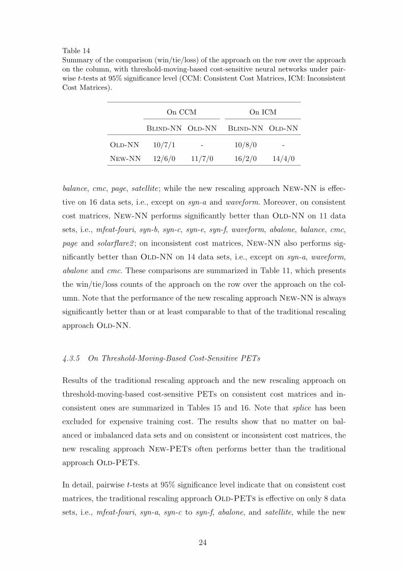
Table 14Summary of the comparison (win/tie/loss) of the approach on the row over the approachon the column, with threshold-moving-based cost-sensitive neural networks under pair-wise t-tests at 95% significance level (CCM: Consistent Cost Matrices, ICM: InconsistentCost Matrices).

On CCM On ICM

Blind-NN Old-NN Blind-NN Old-NN

Old-NN 10/7/1 - 10/8/0 -

New-NN 12/6/0 11/7/0 16/2/0 14/4/0

balance, cmc, page, satellite; while the new rescaling approach New-NN is effec-

tive on 16 data sets, i.e., except on syn-a and waveform. Moreover, on consistent

cost matrices, New-NN performs significantly better than Old-NN on 11 data

sets, i.e., mfeat-fouri, syn-b, syn-c, syn-e, syn-f, waveform, abalone, balance, cmc,

page and solarflare2 ; on inconsistent cost matrices, New-NN also performs sig-

nificantly better than Old-NN on 14 data sets, i.e., except on syn-a, waveform,

abalone and cmc. These comparisons are summarized in Table 11, which presents

the win/tie/loss counts of the approach on the row over the approach on the col-

umn. Note that the performance of the new rescaling approach New-NN is always

significantly better than or at least comparable to that of the traditional rescaling

approach Old-NN.

4.3.5 On Threshold-Moving-Based Cost-Sensitive PETs

Results of the traditional rescaling approach and the new rescaling approach on

threshold-moving-based cost-sensitive PETs on consistent cost matrices and in-

consistent ones are summarized in Tables 15 and 16. Note that splice has been

excluded for expensive training cost. The results show that no matter on bal-

anced or imbalanced data sets and on consistent or inconsistent cost matrices, the

new rescaling approach New-PETs often performs better than the traditional

approach Old-PETs.

In detail, pairwise t-tests at 95% significance level indicate that on consistent cost

matrices, the traditional rescaling approach Old-PETs is effective on only 8 data

sets, i.e., mfeat-fouri, syn-a, syn-c to syn-f, abalone, and satellite, while the new

24

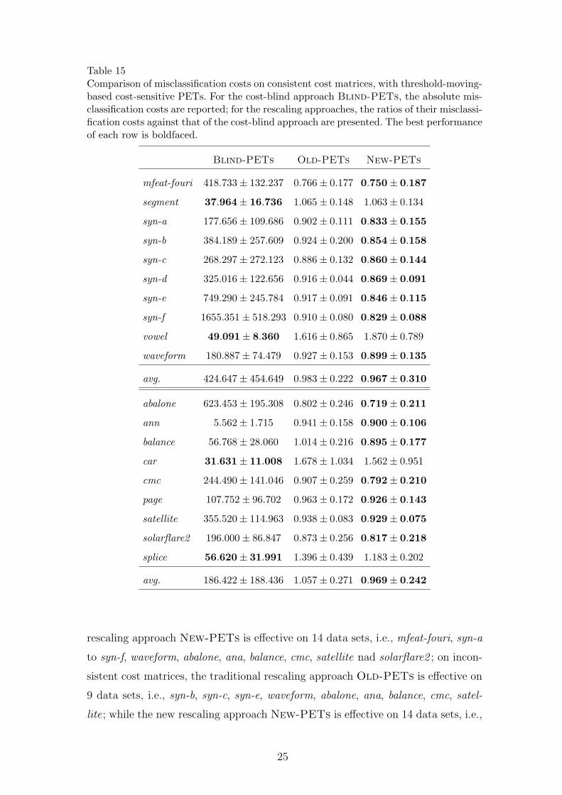
Table 15Comparison of misclassification costs on consistent cost matrices, with threshold-moving-based cost-sensitive PETs. For the cost-blind approach Blind-PETs, the absolute mis-classification costs are reported; for the rescaling approaches, the ratios of their misclassi-fication costs against that of the cost-blind approach are presented. The best performanceof each row is boldfaced.

Blind-PETs Old-PETs New-PETs

mfeat-fouri 418.733± 132.237 0.766± 0.177 0.750± 0.187

segment 37.964± 16.736 1.065± 0.148 1.063± 0.134

syn-a 177.656± 109.686 0.902± 0.111 0.833± 0.155

syn-b 384.189± 257.609 0.924± 0.200 0.854± 0.158

syn-c 268.297± 272.123 0.886± 0.132 0.860± 0.144

syn-d 325.016± 122.656 0.916± 0.044 0.869± 0.091

syn-e 749.290± 245.784 0.917± 0.091 0.846± 0.115

syn-f 1655.351± 518.293 0.910± 0.080 0.829± 0.088

vowel 49.091± 8.360 1.616± 0.865 1.870± 0.789

waveform 180.887± 74.479 0.927± 0.153 0.899± 0.135

avg. 424.647± 454.649 0.983± 0.222 0.967± 0.310

abalone 623.453± 195.308 0.802± 0.246 0.719± 0.211

ann 5.562± 1.715 0.941± 0.158 0.900± 0.106

balance 56.768± 28.060 1.014± 0.216 0.895± 0.177

car 31.631± 11.008 1.678± 1.034 1.562± 0.951

cmc 244.490± 141.046 0.907± 0.259 0.792± 0.210

page 107.752± 96.702 0.963± 0.172 0.926± 0.143

satellite 355.520± 114.963 0.938± 0.083 0.929± 0.075

solarflare2 196.000± 86.847 0.873± 0.256 0.817± 0.218

splice 56.620± 31.991 1.396± 0.439 1.183± 0.202

avg. 186.422± 188.436 1.057± 0.271 0.969± 0.242

rescaling approach New-PETs is effective on 14 data sets, i.e., mfeat-fouri, syn-a

to syn-f, waveform, abalone, ana, balance, cmc, satellite nad solarflare2 ; on incon-

sistent cost matrices, the traditional rescaling approach Old-PETs is effective on

9 data sets, i.e., syn-b, syn-c, syn-e, waveform, abalone, ana, balance, cmc, satel-

lite; while the new rescaling approach New-PETs is effective on 14 data sets, i.e.,

25

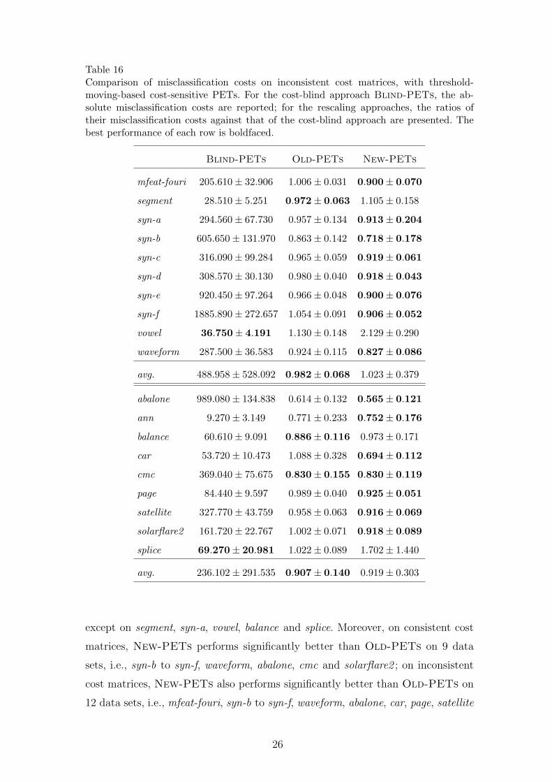
Table 16Comparison of misclassification costs on inconsistent cost matrices, with threshold-moving-based cost-sensitive PETs. For the cost-blind approach Blind-PETs, the ab-solute misclassification costs are reported; for the rescaling approaches, the ratios oftheir misclassification costs against that of the cost-blind approach are presented. Thebest performance of each row is boldfaced.

Blind-PETs Old-PETs New-PETs

mfeat-fouri 205.610± 32.906 1.006± 0.031 0.900± 0.070

segment 28.510± 5.251 0.972± 0.063 1.105± 0.158

syn-a 294.560± 67.730 0.957± 0.134 0.913± 0.204

syn-b 605.650± 131.970 0.863± 0.142 0.718± 0.178

syn-c 316.090± 99.284 0.965± 0.059 0.919± 0.061

syn-d 308.570± 30.130 0.980± 0.040 0.918± 0.043

syn-e 920.450± 97.264 0.966± 0.048 0.900± 0.076

syn-f 1885.890± 272.657 1.054± 0.091 0.906± 0.052

vowel 36.750± 4.191 1.130± 0.148 2.129± 0.290

waveform 287.500± 36.583 0.924± 0.115 0.827± 0.086

avg. 488.958± 528.092 0.982± 0.068 1.023± 0.379

abalone 989.080± 134.838 0.614± 0.132 0.565± 0.121

ann 9.270± 3.149 0.771± 0.233 0.752± 0.176

balance 60.610± 9.091 0.886± 0.116 0.973± 0.171

car 53.720± 10.473 1.088± 0.328 0.694± 0.112

cmc 369.040± 75.675 0.830± 0.155 0.830± 0.119

page 84.440± 9.597 0.989± 0.040 0.925± 0.051

satellite 327.770± 43.759 0.958± 0.063 0.916± 0.069

solarflare2 161.720± 22.767 1.002± 0.071 0.918± 0.089

splice 69.270± 20.981 1.022± 0.089 1.702± 1.440

avg. 236.102± 291.535 0.907± 0.140 0.919± 0.303

except on segment, syn-a, vowel, balance and splice. Moreover, on consistent cost

matrices, New-PETs performs significantly better than Old-PETs on 9 data

sets, i.e., syn-b to syn-f, waveform, abalone, cmc and solarflare2 ; on inconsistent

cost matrices, New-PETs also performs significantly better than Old-PETs on

12 data sets, i.e., mfeat-fouri, syn-b to syn-f, waveform, abalone, car, page, satellite

26

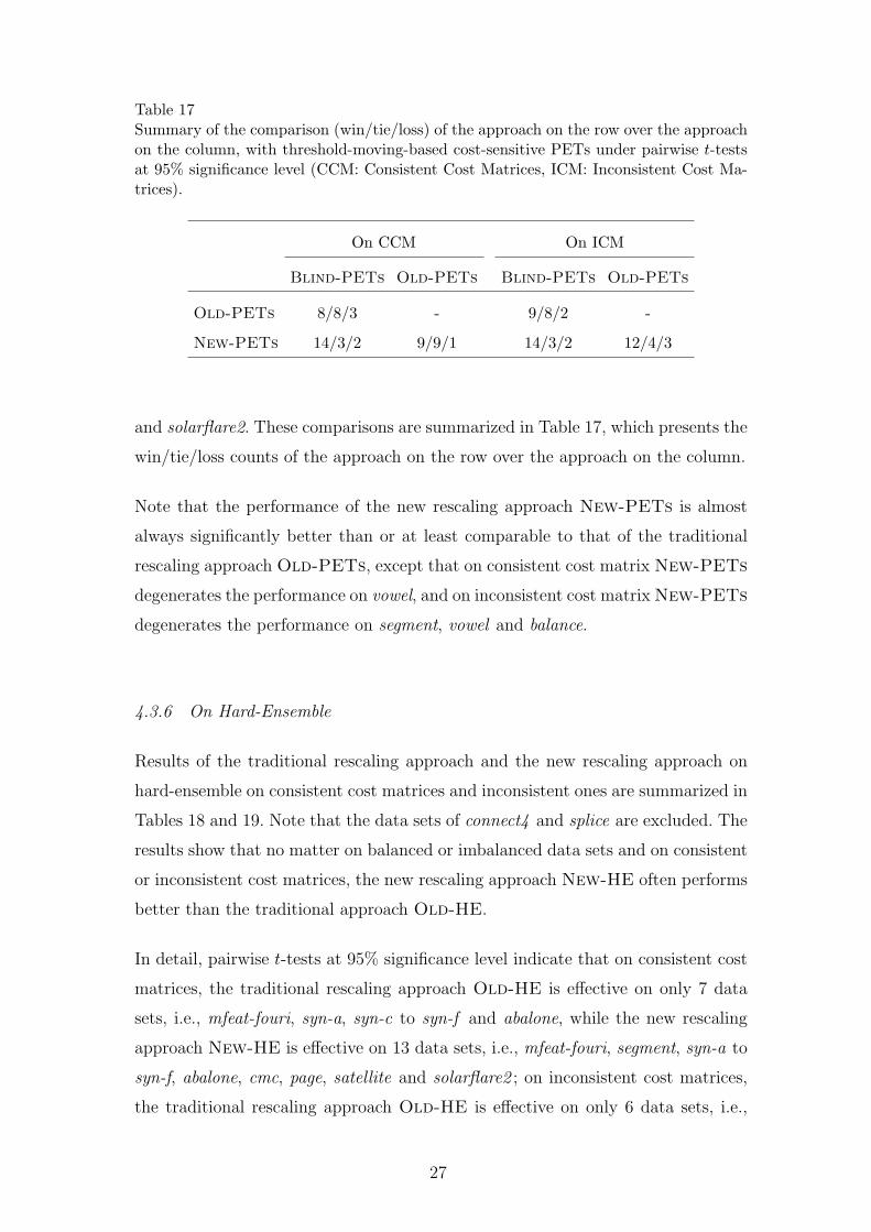
Table 17Summary of the comparison (win/tie/loss) of the approach on the row over the approachon the column, with threshold-moving-based cost-sensitive PETs under pairwise t-testsat 95% significance level (CCM: Consistent Cost Matrices, ICM: Inconsistent Cost Ma-trices).

On CCM On ICM

Blind-PETs Old-PETs Blind-PETs Old-PETs

Old-PETs 8/8/3 - 9/8/2 -

New-PETs 14/3/2 9/9/1 14/3/2 12/4/3

and solarflare2. These comparisons are summarized in Table 17, which presents the

win/tie/loss counts of the approach on the row over the approach on the column.

Note that the performance of the new rescaling approach New-PETs is almost

always significantly better than or at least comparable to that of the traditional

rescaling approach Old-PETs, except that on consistent cost matrix New-PETs

degenerates the performance on vowel, and on inconsistent cost matrix New-PETs

degenerates the performance on segment, vowel and balance.

4.3.6 On Hard-Ensemble

Results of the traditional rescaling approach and the new rescaling approach on

hard-ensemble on consistent cost matrices and inconsistent ones are summarized in

Tables 18 and 19. Note that the data sets of connect4 and splice are excluded. The

results show that no matter on balanced or imbalanced data sets and on consistent

or inconsistent cost matrices, the new rescaling approach New-HE often performs

better than the traditional approach Old-HE.

In detail, pairwise t-tests at 95% significance level indicate that on consistent cost

matrices, the traditional rescaling approach Old-HE is effective on only 7 data

sets, i.e., mfeat-fouri, syn-a, syn-c to syn-f and abalone, while the new rescaling

approach New-HE is effective on 13 data sets, i.e., mfeat-fouri, segment, syn-a to

syn-f, abalone, cmc, page, satellite and solarflare2 ; on inconsistent cost matrices,

the traditional rescaling approach Old-HE is effective on only 6 data sets, i.e.,

27

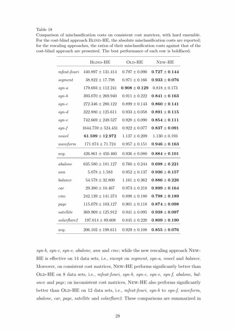
Table 18Comparison of misclassification costs on consistent cost matrices, with hard ensemble.For the cost-blind approach Blind-HE, the absolute misclassification costs are reported;for the rescaling approaches, the ratios of their misclassification costs against that of thecost-blind approach are presented. The best performance of each row is boldfaced.

Blind-HE Old-HE New-HE

mfeat-fouri 440.897± 131.414 0.797± 0.090 0.727± 0.144

segment 38.822± 17.798 0.971± 0.166 0.933± 0.076

syn-a 179.693± 112.241 0.908± 0.129 0.818± 0.173

syn-b 393.070± 269.940 0.911± 0.222 0.841± 0.163

syn-c 272.346± 280.122 0.899± 0.143 0.860± 0.141

syn-d 322.880± 125.611 0.933± 0.058 0.891± 0.115

syn-e 742.669± 249.527 0.928± 0.090 0.854± 0.111

syn-f 1644.759± 524.431 0.922± 0.077 0.837± 0.091

vowel 61.599± 12.972 1.137± 0.209 1.130± 0.193

waveform 171.874± 71.724 0.957± 0.151 0.946± 0.163

avg. 426.861± 450.460 0.936± 0.080 0.884± 0.101

abalone 635.580± 181.127 0.760± 0.244 0.698± 0.221

ann 5.078± 1.583 0.952± 0.137 0.936± 0.157

balance 54.578± 32.800 1.161± 0.362 0.886± 0.226

car 29.380± 10.467 0.973± 0.218 0.899± 0.164

cmc 242.139± 141.374 0.898± 0.180 0.798± 0.189

page 115.079± 103.127 0.901± 0.118 0.874± 0.098

satellite 369.969± 125.912 0.941± 0.095 0.938± 0.097

solarflare2 197.014± 89.608 0.845± 0.220 0.809± 0.190

avg. 206.102± 198.611 0.929± 0.108 0.855± 0.076

syn-b, syn-c, syn-e, abalone, ann and cmc; while the new rescaling approach New-

HE is effective on 14 data sets, i.e., except on segment, syn-a, vowel and balance.

Moreover, on consistent cost matrices, New-HE performs significantly better than

Old-HE on 8 data sets, i.e., mfeat-fouri, syn-b, syn-c, syn-e, syn-f, abalone, bal-

ance and page; on inconsistent cost matrices, New-HE also performs significantly

better than Old-HE on 12 data sets, i.e., mfeat-fouri, syn-b to syn-f, waveform,

abalone, car, page, satellite and solarflare2. These comparisons are summarized in

28

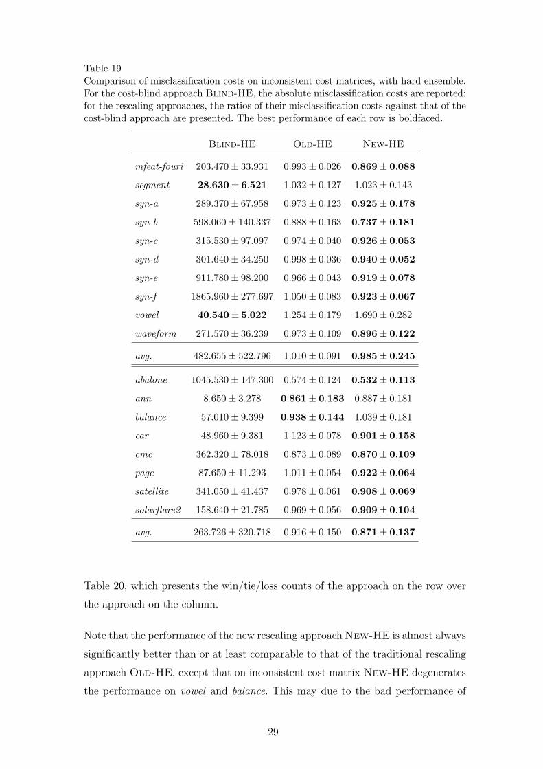
Table 19Comparison of misclassification costs on inconsistent cost matrices, with hard ensemble.For the cost-blind approach Blind-HE, the absolute misclassification costs are reported;for the rescaling approaches, the ratios of their misclassification costs against that of thecost-blind approach are presented. The best performance of each row is boldfaced.

Blind-HE Old-HE New-HE

mfeat-fouri 203.470± 33.931 0.993± 0.026 0.869± 0.088

segment 28.630± 6.521 1.032± 0.127 1.023± 0.143

syn-a 289.370± 67.958 0.973± 0.123 0.925± 0.178

syn-b 598.060± 140.337 0.888± 0.163 0.737± 0.181

syn-c 315.530± 97.097 0.974± 0.040 0.926± 0.053

syn-d 301.640± 34.250 0.998± 0.036 0.940± 0.052

syn-e 911.780± 98.200 0.966± 0.043 0.919± 0.078

syn-f 1865.960± 277.697 1.050± 0.083 0.923± 0.067

vowel 40.540± 5.022 1.254± 0.179 1.690± 0.282

waveform 271.570± 36.239 0.973± 0.109 0.896± 0.122

avg. 482.655± 522.796 1.010± 0.091 0.985± 0.245

abalone 1045.530± 147.300 0.574± 0.124 0.532± 0.113

ann 8.650± 3.278 0.861± 0.183 0.887± 0.181

balance 57.010± 9.399 0.938± 0.144 1.039± 0.181

car 48.960± 9.381 1.123± 0.078 0.901± 0.158

cmc 362.320± 78.018 0.873± 0.089 0.870± 0.109

page 87.650± 11.293 1.011± 0.054 0.922± 0.064

satellite 341.050± 41.437 0.978± 0.061 0.908± 0.069

solarflare2 158.640± 21.785 0.969± 0.056 0.909± 0.104

avg. 263.726± 320.718 0.916± 0.150 0.871± 0.137

Table 20, which presents the win/tie/loss counts of the approach on the row over

the approach on the column.

Note that the performance of the new rescaling approach New-HE is almost always

significantly better than or at least comparable to that of the traditional rescaling

approach Old-HE, except that on inconsistent cost matrix New-HE degenerates

the performance on vowel and balance. This may due to the bad performance of

29

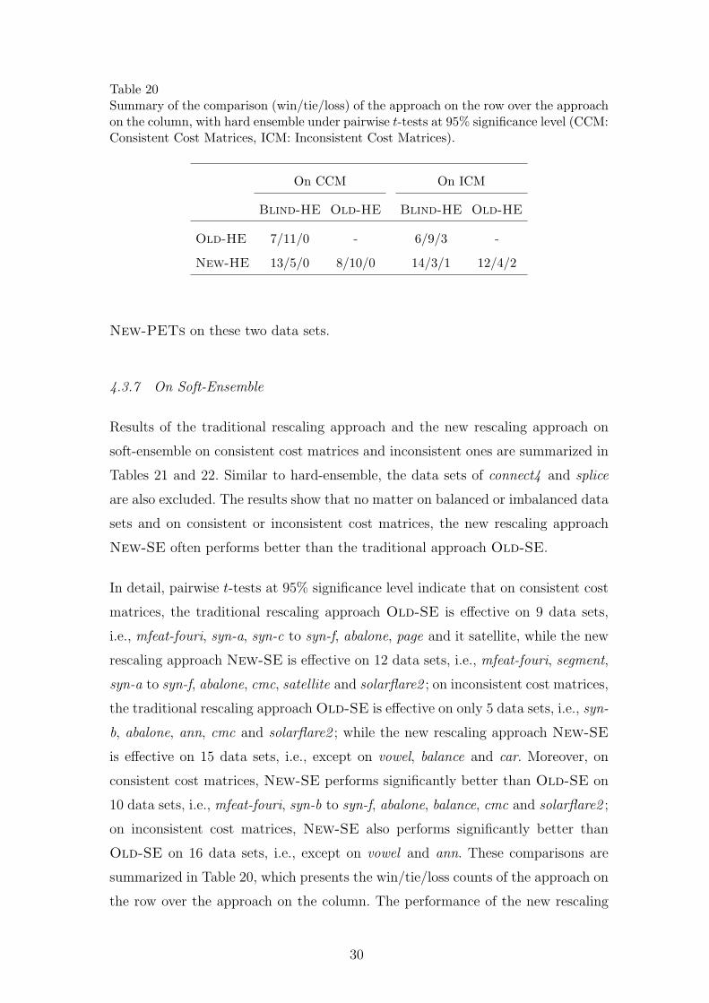
Table 20Summary of the comparison (win/tie/loss) of the approach on the row over the approachon the column, with hard ensemble under pairwise t-tests at 95% significance level (CCM:Consistent Cost Matrices, ICM: Inconsistent Cost Matrices).

On CCM On ICM

Blind-HE Old-HE Blind-HE Old-HE

Old-HE 7/11/0 - 6/9/3 -

New-HE 13/5/0 8/10/0 14/3/1 12/4/2

New-PETs on these two data sets.

4.3.7 On Soft-Ensemble

Results of the traditional rescaling approach and the new rescaling approach on

soft-ensemble on consistent cost matrices and inconsistent ones are summarized in

Tables 21 and 22. Similar to hard-ensemble, the data sets of connect4 and splice

are also excluded. The results show that no matter on balanced or imbalanced data

sets and on consistent or inconsistent cost matrices, the new rescaling approach

New-SE often performs better than the traditional approach Old-SE.

In detail, pairwise t-tests at 95% significance level indicate that on consistent cost

matrices, the traditional rescaling approach Old-SE is effective on 9 data sets,

i.e., mfeat-fouri, syn-a, syn-c to syn-f, abalone, page and it satellite, while the new

rescaling approach New-SE is effective on 12 data sets, i.e., mfeat-fouri, segment,

syn-a to syn-f, abalone, cmc, satellite and solarflare2 ; on inconsistent cost matrices,

the traditional rescaling approach Old-SE is effective on only 5 data sets, i.e., syn-

b, abalone, ann, cmc and solarflare2 ; while the new rescaling approach New-SE

is effective on 15 data sets, i.e., except on vowel, balance and car. Moreover, on

consistent cost matrices, New-SE performs significantly better than Old-SE on

10 data sets, i.e., mfeat-fouri, syn-b to syn-f, abalone, balance, cmc and solarflare2 ;

on inconsistent cost matrices, New-SE also performs significantly better than

Old-SE on 16 data sets, i.e., except on vowel and ann. These comparisons are

summarized in Table 20, which presents the win/tie/loss counts of the approach on

the row over the approach on the column. The performance of the new rescaling

30

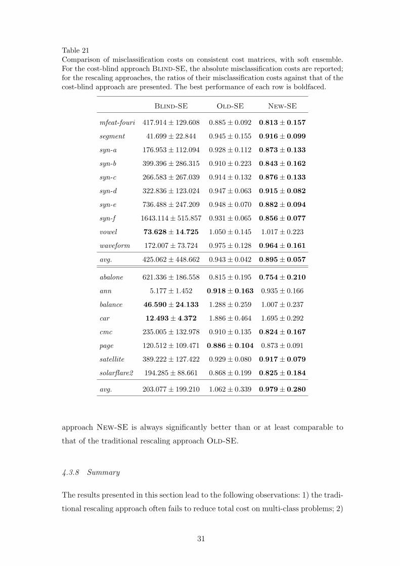
Table 21Comparison of misclassification costs on consistent cost matrices, with soft ensemble.For the cost-blind approach Blind-SE, the absolute misclassification costs are reported;for the rescaling approaches, the ratios of their misclassification costs against that of thecost-blind approach are presented. The best performance of each row is boldfaced.

Blind-SE Old-SE New-SE

mfeat-fouri 417.914± 129.608 0.885± 0.092 0.813± 0.157

segment 41.699± 22.844 0.945± 0.155 0.916± 0.099

syn-a 176.953± 112.094 0.928± 0.112 0.873± 0.133

syn-b 399.396± 286.315 0.910± 0.223 0.843± 0.162

syn-c 266.583± 267.039 0.914± 0.132 0.876± 0.133

syn-d 322.836± 123.024 0.947± 0.063 0.915± 0.082

syn-e 736.488± 247.209 0.948± 0.070 0.882± 0.094

syn-f 1643.114± 515.857 0.931± 0.065 0.856± 0.077

vowel 73.628± 14.725 1.050± 0.145 1.017± 0.223

waveform 172.007± 73.724 0.975± 0.128 0.964± 0.161

avg. 425.062± 448.662 0.943± 0.042 0.895± 0.057

abalone 621.336± 186.558 0.815± 0.195 0.754± 0.210

ann 5.177± 1.452 0.918± 0.163 0.935± 0.166

balance 46.590± 24.133 1.288± 0.259 1.007± 0.237

car 12.493± 4.372 1.886± 0.464 1.695± 0.292

cmc 235.005± 132.978 0.910± 0.135 0.824± 0.167

page 120.512± 109.471 0.886± 0.104 0.873± 0.091

satellite 389.222± 127.422 0.929± 0.080 0.917± 0.079

solarflare2 194.285± 88.661 0.868± 0.199 0.825± 0.184

avg. 203.077± 199.210 1.062± 0.339 0.979± 0.280

approach New-SE is always significantly better than or at least comparable to

that of the traditional rescaling approach Old-SE.

4.3.8 Summary

The results presented in this section lead to the following observations: 1) the tradi-

tional rescaling approach often fails to reduce total cost on multi-class problems; 2)

31

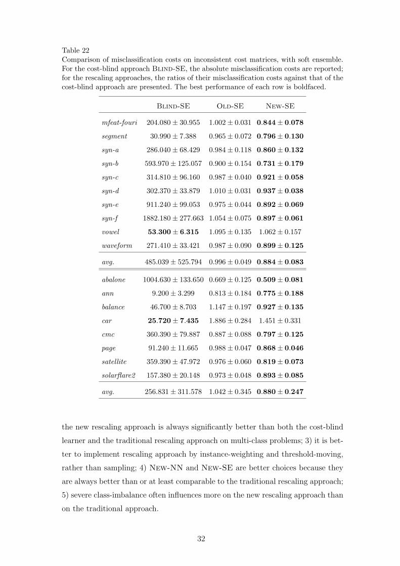
Table 22Comparison of misclassification costs on inconsistent cost matrices, with soft ensemble.For the cost-blind approach Blind-SE, the absolute misclassification costs are reported;for the rescaling approaches, the ratios of their misclassification costs against that of thecost-blind approach are presented. The best performance of each row is boldfaced.

Blind-SE Old-SE New-SE

mfeat-fouri 204.080± 30.955 1.002± 0.031 0.844± 0.078

segment 30.990± 7.388 0.965± 0.072 0.796± 0.130

syn-a 286.040± 68.429 0.984± 0.118 0.860± 0.132

syn-b 593.970± 125.057 0.900± 0.154 0.731± 0.179

syn-c 314.810± 96.160 0.987± 0.040 0.921± 0.058

syn-d 302.370± 33.879 1.010± 0.031 0.937± 0.038

syn-e 911.240± 99.053 0.975± 0.044 0.892± 0.069

syn-f 1882.180± 277.663 1.054± 0.075 0.897± 0.061

vowel 53.300± 6.315 1.095± 0.135 1.062± 0.157

waveform 271.410± 33.421 0.987± 0.090 0.899± 0.125

avg. 485.039± 525.794 0.996± 0.049 0.884± 0.083

abalone 1004.630± 133.650 0.669± 0.125 0.509± 0.081

ann 9.200± 3.299 0.813± 0.184 0.775± 0.188

balance 46.700± 8.703 1.147± 0.197 0.927± 0.135

car 25.720± 7.435 1.886± 0.284 1.451± 0.331

cmc 360.390± 79.887 0.887± 0.088 0.797± 0.125

page 91.240± 11.665 0.988± 0.047 0.868± 0.046

satellite 359.390± 47.972 0.976± 0.060 0.819± 0.073

solarflare2 157.380± 20.148 0.973± 0.048 0.893± 0.085

avg. 256.831± 311.578 1.042± 0.345 0.880± 0.247

the new rescaling approach is always significantly better than both the cost-blind

learner and the traditional rescaling approach on multi-class problems; 3) it is bet-

ter to implement rescaling approach by instance-weighting and threshold-moving,

rather than sampling; 4) New-NN and New-SE are better choices because they

are always better than or at least comparable to the traditional rescaling approach;

5) severe class-imbalance often influences more on the new rescaling approach than

on the traditional approach.

32

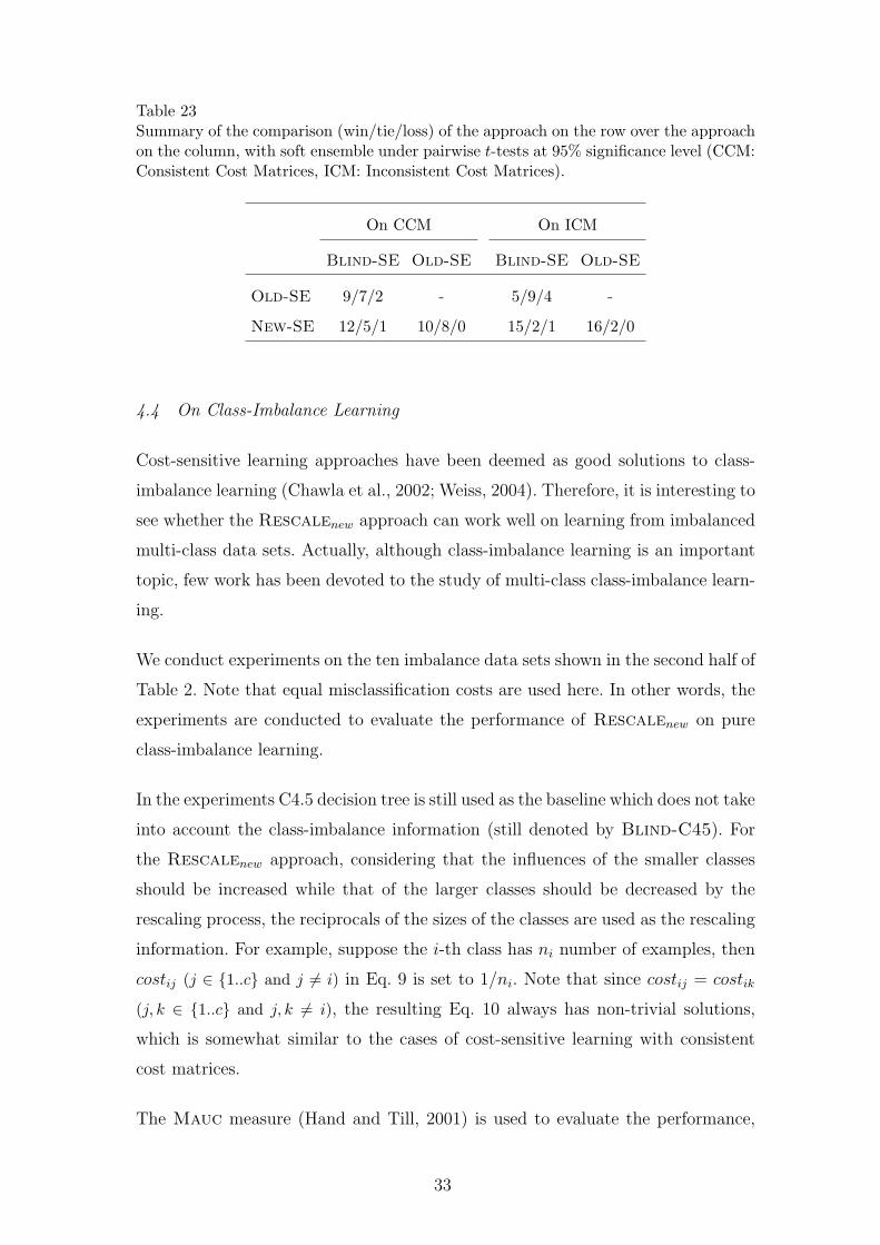
Table 23Summary of the comparison (win/tie/loss) of the approach on the row over the approachon the column, with soft ensemble under pairwise t-tests at 95% significance level (CCM:Consistent Cost Matrices, ICM: Inconsistent Cost Matrices).

On CCM On ICM

Blind-SE Old-SE Blind-SE Old-SE

Old-SE 9/7/2 - 5/9/4 -

New-SE 12/5/1 10/8/0 15/2/1 16/2/0

4.4 On Class-Imbalance Learning

Cost-sensitive learning approaches have been deemed as good solutions to class-

imbalance learning (Chawla et al., 2002; Weiss, 2004). Therefore, it is interesting to

see whether the Rescalenew approach can work well on learning from imbalanced

multi-class data sets. Actually, although class-imbalance learning is an important

topic, few work has been devoted to the study of multi-class class-imbalance learn-

ing.

We conduct experiments on the ten imbalance data sets shown in the second half of

Table 2. Note that equal misclassification costs are used here. In other words, the

experiments are conducted to evaluate the performance of Rescalenew on pure

class-imbalance learning.

In the experiments C4.5 decision tree is still used as the baseline which does not take

into account the class-imbalance information (still denoted by Blind-C45). For

the Rescalenew approach, considering that the influences of the smaller classes

should be increased while that of the larger classes should be decreased by the

rescaling process, the reciprocals of the sizes of the classes are used as the rescaling

information. For example, suppose the i-th class has ni number of examples, then

costij (j ∈ {1..c} and j 6= i) in Eq. 9 is set to 1/ni. Note that since costij = costik

(j, k ∈ {1..c} and j, k 6= i), the resulting Eq. 10 always has non-trivial solutions,

which is somewhat similar to the cases of cost-sensitive learning with consistent

cost matrices.

The Mauc measure (Hand and Till, 2001) is used to evaluate the performance,

33

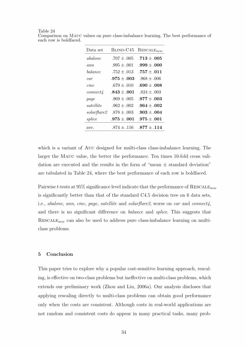
Table 24Comparison on Mauc values on pure class-imbalance learning. The best performance ofeach row is boldfaced.

Data set Blind-C45 Rescalenew

abalone .707± .005 .713± .005ann .995± .001 .999± .000balance .752± .013 .757± .011car .975± .003 .968± .006cmc .679± .010 .690± .008connect4 .843± .001 .824± .003page .969± .005 .977± .003satellite .962± .002 .964± .002solarflare2 .878± .003 .903± .004splice .975± .001 .975± .001

ave. .874± .116 .877± .114

which is a variant of Auc designed for multi-class class-imbalance learning. The

larger the Mauc value, the better the performance. Ten times 10-fold cross vali-

dation are executed and the results in the form of “mean ± standard deviation”

are tabulated in Table 24, where the best performance of each row is boldfaced.

Pairwise t-tests at 95% significance level indicate that the performance of Rescalenew

is significantly better than that of the standard C4.5 decision tree on 6 data sets,

i.e., abalone, ann, cmc, page, satellite and solarflare2, worse on car and connect4,

and there is no significant difference on balance and splice. This suggests that

Rescalenew can also be used to address pure class-imbalance learning on multi-

class problems.

5 Conclusion

This paper tries to explore why a popular cost-sensitive learning approach, rescal-

ing, is effective on two-class problems but ineffective on multi-class problems, which

extends our preliminary work (Zhou and Liu, 2006a). Our analysis discloses that

applying rescaling directly to multi-class problems can obtain good performance

only when the costs are consistent. Although costs in real-world applications are

not random and consistent costs do appear in many practical tasks, many prob-

34

lems are with inconsistent costs. We advocate that the examination of the cost

consistency should be taken as a sanity check for the rescaling approach. When

the check is passed, rescaling can be executed directly; otherwise rescaling should

be executed after decomposing the multi-class problem into a series of two-class

problems. Empirical study shows that the new proposal is not only helpful to

multi-class cost-sensitive learning, but also useful in multi-class class-imbalance

learning.

Unequal misclassification costs and class-imbalance often occur simultaneously.

How to rescale the classes under this situation, however, remains an open problem

(Liu and Zhou, 2006). Our empirical results coincide with Liu and Zhou (2006) on

that when the class-imbalance is not serious, using the cost information to rescale

the classes can work well on most data sets; but this could not apply to seriously

imbalanced data sets. Exploring the ground under this observation and designing

appropriate rescaling schemes for such cases are important future issues.

This paper focuses on the rescaling approach. Note that in addition to rescaling,

there are also other kinds of cost-sensitive learning approaches. However, as men-

tioned before, only a few studies dedicated to multi-class cost-sensitive learning

(Abe et al., 2004; Lozano and Abe, 2008; Zhang and Zhou, 2008; Zhou and Liu,

2006b). Although multi-class problems can be converted into a series of two-class

problems to solve, users usually favor a more direct solution. So, investigating

multi-class cost-sensitive learning approaches without decomposition is an impor-

tant future work. In most cost-sensitive learning studies, the cost matrices are usu-

ally fixed, while in some real-world tasks the costs may change due to many reasons.

Designing effective methods for cost-sensitive learning with variable cost matrices

is another interesting issue for future work. Furthermore, developing powerful tools

for visually evaluating multi-class cost-sensitive learning approaches, such as the

Roc and cost curves for two-class cases, is also an interesting future issue.

35

Acknowledgments

We want to thank anonymous reviewers for helpful comments and suggestions,

and Qi Qian for proof-reading the paper. This work was supported by the Na-

tional Science Foundation of China (60635030, 60721002) and the Jiangsu Science

Foundation (BK2008018).

References

Abe, N., Zadrozny, B., Langford, J., 2004. An iterative method for multi-class

cost-sensitive learning. In: Proceedings of the 10th ACM SIGKDD International

Conference on Knowledge Discovery and Data Mining. Seattle, WA, pp. 3–11.

Allwein, E. L., Schapire, R. E., Singer, Y., 2000. Reducing multiclass to binary: A

unifying approach for margin classifiers. Journal of Machine Learning Research

1, 113–141.

Blake, C., Keogh, E., Merz, C. J., 1998. UCI repository of machine learning

databases. [http://www.ics.uci.edu/∼mlearn/MLRepository.html], Department

of Information and Computer Science, University of California, Irvine, CA.

Brefeld, U., Geibel, P., Wysotzki, F., 2003. Support vector machines with example

dependent costs. In: Proceedings of the 14th European Conference on Machine

Learning. Cavtat-Dubrovnik, Croatia, pp. 23–34.

Breiman, L., Friedman, J. H., Olsen, R. A., Stone, C. J., 1984. Classification and

Regression Trees. Wadsworth, Belmont, CA.

Cebe, M., Gunduz-Demir, C., 2007. Test-cost sensitive classification based on con-

ditioned loss functions. In: Proceeding of the 18th European Conference on Ma-

chine Learning. Warsaw, Poland, pp. 551–558.

Chai, X., Deng, L., Yang, Q., Ling, C. X., 2004. Test-cost sensitive naive bayes

classification. In: Proceeding of the 4th IEEE International Conference on Data

Mining. Brighton, UK, pp. 51–58.

Chawla, N. V., Bowyer, K. W., Hall, L. O., Kegelmeyer, W. P., 2002. SMOTE:

Synthetic minority over-sampling technique. Journal of Artificial Intelligence Re-

36

search 16, 321–357.

Domingos, P., 1999. MetaCost: A general method for making classifiers cost-

sensitive. In: Proceedings of the 5th ACM SIGKDD International Conference

on Knowledge Discovery and Data Mining. San Diego, CA, pp. 155–164.

Drummond, C., Holte, R. C., 2000. Explicitly representing expected cost: An al-

ternative to ROC representation. In: Proceedings of the 6th ACM SIGKDD In-

ternational Conference on Knowledge Discovery and Data Mining. Boston, MA,

pp. 198–207.

Drummond, C., Holte, R. C., 2003. C4.5, class imbalance, and cost sensitivity:

Why under-sampling beats over-sampling. In: Working Notes of the ICML’03

Workshop on Learning from Imbalanced Data Sets. Washington, DC.

Elkan, C., 2001. The foundations of cost-senstive learning. In: Proceedings of the

17th International Joint Conference on Artificial Intelligence. Seattle, WA, pp.

973–978.

Hand, D. J., Till, R. J., 2001. A simple generalisation of the area under the ROC

curve for multiple class classification problems. Machine Learning 45 (2), 171–

186.

Ling, C. X., Yang, Q., Wang, J., Zhang, S., 2004. Decision trees with minimal costs.

In: Proceedings of the 21st International Conference on Machine Learning. Banff,

Canada, pp. 69–76.

Liu, X.-Y., Zhou, Z.-H., 2006. The influence of class imbalance on cost-sensitive

learning: An empirical study. In: Proceedings of the 6th IEEE International

Conference on Data Mining. Hong Kong, China, pp. 970–974.

Lozano, A. C., Abe, N., 2008. Multi-class cost-sensitive boosting with p-norm loss

functions. In: Proceedings of the 14th ACM SIGKDD International Conference

on Knowledge Discovery and Data Mining. Las Vegas, NV, pp. 506–514.

Maloof, M. A., 2003. Learning when data sets are imbalanced and when costs are

unequal and unknown. In: Working Notes of the ICML’03 Workshop on Learning

from Imbalanced Data Sets. Washington, DC.

Margineantu, D., 2001. Methods for cost-sensitive learning. Ph.D. thesis, Depart-

ment of Computer Science, Oregon State University, Corvallis, OR.

Masnadi-Shirazi, H., Vasconcelos, N., 2007. Asymmetric Boosting. In: Proceeding

37

of the 24th International Conference on Machine Learning. Corvallis, OR, pp.

609–619.

Provost, F., Domingos, P., 2003. Tree induction for probability-based ranking. Ma-

chine Learning 52 (3), 199–215.

Saitta, L. (Ed.), 2000. Machine Learning - A Technological Roadmap. University

of Amsterdam, The Netherland.

Ting, K. M., 2002. An instance-weighting method to induce cost-sensitive trees.

IEEE Transactions on Knowledge and Data Engineering 14 (3), 659–665.

Turney, P. D., 2000. Types of cost in inductive concept learning. In: Proceedings of

the ICML’2000 Workshop on Cost-Sensitive Learning. Stanford, CA, pp. 15–21.

Weiss, G. M., 2004. Mining with rarity - problems and solutions: A unifying frame-

work. SIGKDD Explorations 6 (1), 7–19.

Witten, I. H., Frank, E., 2005. Data Mining: Practical Machine Learning Tools

and Techniques with Java Implementations, 2nd Edition. Morgan Kaufmann,

San Francisco, CA.

Zadrozny, B., Elkan, C., 2001. Learning and making decisions when costs and prob-

abilities are both unknown. In: Proceedings of the 7th ACM SIGKDD Interna-

tional Conference on Knowledge Discovery and Data Mining. San Francisco, CA,

pp. 204–213.

Zadrozny, B., Langford, J., Abe, N., 2002. A simple method for cost-sensitive learn-

ing. Tech. rep., IBM.

Zhang, Y., Zhou, Z.-H., 2008. Cost-sensitive face recognition. In: Proceedings of

the IEEE Computer Society Conference on Computer Vision and Pattern Recog-

nition. Anchorage, AK.

Zhou, Z.-H., Liu, X.-Y., 2006a. On multi-class cost-sensitive learning. In: Proceed-

ing of the 21st National Conference on Artificial Intelligence. Boston, WA, pp.

567–572.

Zhou, Z.-H., Liu, X.-Y., 2006b. Training cost-sensitive neural networks with meth-

ods addressing the class imbalance problem. IEEE Transactions on Knowledge

and Data Engineering 18 (1), 63–77.

38