TitleOn the Complex WKB Analysis for Products of the AiryFunctions (Methods and Applications for FunctionalEquations)

Author(s) Nakano, Minoru

Citation 数理解析研究所講究録 (1999), 1083: 169-180

Issue Date 1999-02

URL http://hdl.handle.net/2433/62759

Right

Type Departmental Bulletin Paper

Textversion publisher

Kyoto University

On the Complex WKB Analysisfor Products of the Airy Functions

Minoru NAKANO (中野 $\text{實}$: 慶応大学)

Departnent of Mathematics, Faculty of Science and Technology, Keio University.314-1 Hiyoshi, Kohoku, Yokohama, Kanagawa 223-8522, JAPAN

Tel: 045-563-1141, Fax: 045-563-5948, Email: nakano@math.keio.ac.jp

\S 1. Introduction.1.1. We $\infty \mathrm{n}\mathrm{s}\mathrm{i}\mathrm{d}\mathrm{e}\mathrm{r}$ a third order linear ordinary differential equation containing a small pa-

rameter $\epsilon$ :

(1.1) $\epsilon^{3}y’’’+3\epsilon^{2\prime}p_{2}(X)y’+3\epsilon p_{1}(x)y’+\mu)(X)y=0$ , $0<\epsilon\leq\epsilon_{0}$ , $|x|\leq x_{0}$ ,

where $x$ is complex.We suppose that the coefficients of (1.1) are linear functions of $x$ such as

$p_{2}(x)=ax+b,$ $p_{1}(x)=cx+d,$ $n(x)=ex+f$,

where $a,$ $b,$$\cdots,$ $f$ are $\infty \mathrm{m}\mathrm{p}\mathrm{l}\mathrm{e}\mathrm{x}$ constants.

The characteristic equation of (1.1) is given by

(1.2) $k(\lambda, x):=\lambda^{3}+3p2(x)\lambda 2+3p_{1}(x)\lambda+p_{0}(X)=0$ ,

whose roots are $\mathrm{c}\mathrm{a}\mathrm{J}\mathrm{l}\mathrm{e}\mathrm{d}$ the characteristic roots for (1.1) and they are denoted by $\lambda_{j}(x)$ $(j=$$1,2,3)$ . We denote by $D$ a discriminant of the algebraic equation (1.2).

1.2. We give a brief summary on the complex WKB analysis about (1.1).

Definition 1. Zeros of the $di_{SC\dot{n}}minantD$ are called tuming points of the equation (1.1),or a point $x=asati_{Shi}ng\lambda j(a)=\lambda_{l}(a)(j\neq l)$ is a tuming point of the equation (1.1).

$\partial^{2}k(\lambda(x), X)$

The tuming point $xsati_{S}hing\overline{\partial\lambda^{2}}\neq 0$ and $\frac{\partial k(\lambda(x),X)}{\partial x}\neq 0$ are called of simpleorder.

Definition 2. Curves on the $x$-plane determined by

(1.3) $\Re_{\xi_{ji}}(a, X)=0$ , $\xi_{jl(a,X):}=\int_{a}^{x}\{\lambda_{j}(X)-\lambda l(X)\}dX$ , $\lambda_{j}(a)=\lambda_{1}(a)$ $(j\neq l)$

are called Stokes curves of the equation (1.1). Curve8 determined by $\Im\xi_{j}\iota(a, X)=0$ are calledanti-Stokes curves of the equation (1.1). They emerge from the tuming point $x=a$ .

$,Curves\Re\xi_{jl}(a, x)=conSt$. and curves $\Im\xi_{jl}(a, x)=co.nSt$. are called level curves.

Both of Stokes and anti-Stokes curves are level curves of level zero. It is known that Stokescurves of the equation (1.1) emerging from one turning point do not intersect each other exceptfor this turning point and the point at infinity, and a $\mathrm{S}\mathrm{t}\mathrm{o}\mathrm{k}\mathrm{e}\vee \mathrm{s}$ curve of the equation (1.1) doesnot make a loop (Kelly [12]).

数理解析研究所講究録1083巻 1999年 169-180 169

We remark that someone calls curves defined by $\Re.\xi_{J^{\mathit{1}(X)}}a,=0$ anti-Stokes curves, and callscurves defined by $\Im\xi_{jl}(a, X)=0$ Stokes curves. Terminology is sometimes used conversely.

Definition 3. The main terrn $\tilde{y}_{j}(x, \epsilon)$ of a formal $se\tau^{\tau}ieS$ solution of (1.1) is called a formal$WKB_{\mathit{8}O}luti_{on}$ of the equahon (1.1):

(1.4) $\tilde{y}_{j}(X, \xi):=\frac{1}{\sqrt{(\lambda_{j}-\lambda_{j+1})(\lambda_{j}-\lambda_{j2}+)}}(\frac{1}{\epsilon}[_{a}x_{\lambda j(X)dx})(j=1,2,3;\lambda_{4}:=\lambda_{1}, \lambda 5:=\lambda 2)$.

This is derived from the formulae given in Fedoryuk [7], [8] or Nakano et. al. [15].

Lemma 1. There erists an $x- re\dot{\varphi}onDj$ such that the fomal $WKB$ solutions $\tilde{y}_{j}(x, \epsilon)po\mathit{8}sess$

double $asympt_{\mathit{0}}uC$ property

$y_{j}(x, \epsilon)\sim\tilde{y}j(x, \epsilon)$

(1.5) as $xarrow\infty$ in $D_{j}$ for $\epsilon$ ,

(1.6) as $\epsilonarrow 0$ for $x\in D_{j;}$

where $y_{j}(x, \epsilon)$ is a true soluhon of (1.1).

This lemma can be proved by the similar IIaethod used for second order differential equations(Evgrafov-Fedoryuk [5] or Nalcano et. al. [15]).

W-K-B are originated from Wentzel [20], Kramers [13] and Brillouin [4].

Definition 4. The maximal region $D_{j}$ of the $x$ -plane, in which a formd $WKB$ solution$\tilde{y}_{j}(x, \epsilon)$ is an asymptotic expansion of the true solution $y_{j}(X, \xi)_{J}i_{\mathit{8}}$ called a $\lambda_{j^{-}}admis\mathit{8}ible\Gamma e\dot{\varphi}on$

of the equation (1.1).An intersection of three $\lambda_{j}$ -admissible $region\mathit{8}D_{1}\cap D_{2}\cap D_{3}$ is called a canonical region of the

equation (1.1).

The canonical region is the $\max‘$inal region in which three linearly independent solutions$y_{j}(x, \epsilon)_{\mathrm{S}}$

’ of (1.1) possess formal WKB solutions $\tilde{y}_{j}(x, \epsilon)_{\mathrm{S}}$’ as asymptotic solutions. There are

several canonical regions of (1.1) (see \S 6).

In \S 2 it is shown that the equation (1.1) is classified into nine classes and they are shown onthe table. From \S 3 we study mainly about the equation type Ib on the table.

In \S 4 we study location of tuming points and local Stokes curves for the equation type Ib, in\S 5 global Stokes curves are considered and they are shown in several figllres, in \S 6 the canonicalregion, eistence region of three independent solutions with some asymptotic property, are gained,in \S 7 we show that the solution can be represented by the Laplace integral, in \S 8 we give a briefskecth of the Airy functions and in \S 9, the last section, we study relation between solutions ofthe equation type Ib and products of the Airy functions.

This article is a revised edition of Nakano [14].

\S 2. Classification of 3rd order equations.2.1. We can classify the differential equation (1.1) in a six-dimensional space with respect

to the order and numbers of the turning points of (1.1) by using the discriminant $D$ of (1.2).The characteristic equation (1.2) can be reduced to

$(2.1)_{1}$ $\eta^{3}+3P\eta+Q=0$ ,

where

(2.1)2. $\eta:=\lambda+p_{2}(x)$ , $P:=p_{1}(x)-p_{2}(X)^{2}$ , $Q:=2p2(X)^{3}-3p_{2}(X)P1(X)+n)(x)$ .

170

The solutions $\xi$ of $(2.1)_{1}$ are given by the Cardano’s formula as follows:

(2.2)1 $\eta_{1}$$:=\sqrt[3]{\alpha}+\sqrt[3]{\sqrt}$ , $\eta_{2}:=\omega\sqrt[3]{\alpha}+\omega^{2}\sqrt[3]{\beta}$, $\eta_{3}$

$:=\omega^{2}\sqrt[3]{\alpha}+\omega\sqrt[3]{\beta}$ ,

where

$(2.2)_{2}$ a $:= \frac{-Q+\sqrt{D}}{2}$ , $\beta:=\frac{-Q-\sqrt{D}}{2}$ , $D:=4P^{3}+Q^{2}$ .

$‘ D$ ’ is a discriminant of the characteristic equation of (1.2) (and (2.1)) since roots of (1.2)(and (2.1)) coincide at zeros of $D$ , and these zeros are the turning points of (1.1) (see Def. 1).

2.2. The discriminant $D$ is expressed by a polynomial of $x$ as follows:

$D$ $:=4\{p1(X)-p_{2(X)}2\}^{3}+\{(2p2(X)3-3p2(X)p1(X)+p\mathrm{o}(X)\}^{2}$

$=-3p_{2}(x)^{2}p1(x)^{2}+4p_{1}(x)^{3}+4p_{2}(x)^{3}\emptyset(X)-6\prime p_{2}(X)p_{1}(x)n(X)+p_{0}(X)^{2}$

$=(-3b^{2}d^{2}+4d^{3}+4b^{3}f-6bdf+f^{2})$

$+(-6b^{2}cd-6ab\mathrm{C}P+12cd^{2}+4b^{3}e - 6\mathrm{b}\ +\mathrm{l}2ab^{2}f-6b_{C}f-6adf+2ef)_{X}$

$+(-3b^{22}C-12abcd+12c^{2}d-3ad22+12ab^{2}e-6bCe-6ade+e^{2}+12a^{22}bf-6aCf)X$

$+(-6abC^{2}+4c^{32}-6acd+12a^{2}be-6ace+4a^{3}f)_{X^{3}}$

$+a^{2}(-3c^{2}+4ae)x^{4}$ .

Since $D$ is of degree 4, there are at most four roots. By defining constants $a,$ $b,$$\cdots,$ $f$ appro-

priately, we get the following typical examples of the characteristic equations.

REMARK: The mark $‘ 0$ ’ represents a number of $n$-ple zeros. There exists no case where $D$

has only one simple zero, and there exists also no case where $D$ has a -ple zero.

\S 3. The equation Ib.

3.1. Rom now on we are mainly $\infty \mathrm{n}\mathrm{s}\mathrm{i}\mathrm{d}\mathrm{e}\mathrm{r}\mathrm{i}\mathrm{n}\mathrm{g}$ the third order linear ordinary differentialequation of type Ib on the table in 920.2:(3.1) $\epsilon^{3}y’’’-4\epsilon xy’-2y=0$ .

The equation (3.1) has three simple turning points at $x=3/4,$ $\mathrm{a}v/4,$ $\mathrm{a}_{v^{2}}/4(\omega^{3}=1, \omega\neq 1)$

as shown on the table (aee Def. 1), and the point at infinity is an irregular $\sin_{\mathrm{o}}\mathrm{g}\mathrm{a}\mathrm{r}$ point.

171

When $\epsilon=1$ the solutions of (3.1) are $\mathrm{A}\mathrm{i}(X)^{2},$ $\mathrm{A}\mathrm{i}(x)\cdot \mathrm{B}\mathrm{i}(x)$ and $\mathrm{B}\mathrm{i}(X)^{2}$ , where $\mathrm{A}\mathrm{i}(x)$ and$\mathrm{B}\mathrm{i}(x)$ are the Airy functions. The Airy functions are linearly independent solutions of the Airyequation

(3.2) $Y”-xY=0$.

The equation Ib’ has same property as the equation Ib, but we prefer the equation Ib becauseit relates directly to the Airy equation.

The characteristic roots $\lambda:=\lambda_{j}(x)(j=1,2,3)$ for (3.1) are given by

(3.3) $\{$

$\lambda_{1}(x):=\alpha+\frac{4x}{3}1/3.-\alpha 1/3$,

$\lambda_{2}(X):=\omega\alpha 21/3\frac{4x}{3}\cdot\omega\alpha^{-}1/+3$,

$\lambda_{3}(x):=\omega\alpha+1/3\frac{4x}{3}\cdot\omega^{2}\alpha-1/3$ ,

$(\alpha:=1+\sqrt{D}$, $D:=1-( \frac{4x}{3})^{3})$

The formal WKB solutions of (3.1) are got from (1.4)

(3.4) $\tilde{y}_{1}(x, \epsilon)=xe^{\frac{1}{\epsilon}}(1-3\epsilon)/4\epsilon\frac{4}{3}x3/2$ , $\tilde{y}_{2}(X, \epsilon)=x^{-1}/2\epsilon$ , $\tilde{y}_{3}(x, \epsilon)=x(1-3\epsilon)/4\epsilon-e\frac{1}{\in}\frac{4}{3}x3/2$

3.2. In the case of aecond order linear differential equations there are only two characteristicvalues. Then, there is only one difference of them if we take no account of signature. Turningpoints and Stokes curves are determined by this difference (see Def. 1, 2).

However, in the case of higher order differential equations there are many differences of char-acteristic roots, and Stokes curves are determined by these differences. Therefore, Stokes curvesmay cross each other. Indeed, the crossing of Stokes curves happens for the equation (3.1) (seeFig. 1). In this sense the equation (3.1) is a typical example with general property which theg.eneral higher order differential equations possess, nevertheless the equation (3.1) looks verysmple.

Third order equations are studied by, for instance, Aoki et. al. [2], Berk et. al. [3] and Nakanoet. al. [15]. Berk et. al. studied the equation of type Ia introducing a new Stokes curve andshowing that a Stokes phenomenon happens on the new Stokes curve, and computed a Stokesmultiplier. However we need no new Stokes curves and we can get canonical regions withoutnew Stokes curves. We use ‘old’ Stokes curves only (see Theorem 4).

\S 4. Turning points and local Stokes curves.4.1. We can see that every characteristic root $\lambda_{j}(x)$ is obtained by other characteristic roots

by changing arguments and we get the $\mathrm{f}\mathrm{o}\mathrm{U}\mathrm{o}\mathrm{w}\mathrm{i}\mathrm{n}\mathrm{g}$ relations which we call the rotation rules.

Theorem 1. Between characteristic roots the following equations are valid:

(4.1) $\lambda_{1}(x\omega)=\omega^{2}\lambda 3(X)$ , $\lambda_{2}(x\omega)=\omega^{2}\lambda 1(X)$ , $\lambda_{3}(x\omega)=\omega\lambda_{2();}2x$

(4.2) $\lambda_{12}(X)=\omega\lambda 23(x\omega)_{)}$ $\lambda_{23}(X)=\omega\lambda_{3}1(x\omega)$ , $\lambda_{31}(X)=\omega\lambda_{1}2(x\omega)$ ,

where $\omega:=e^{2\pi i/3},$ $\lambda_{jk}(X):=\lambda_{j}(x)-\lambda_{k(X)}$ .PROOF. These rotation rules are easily derived from the definition of $\lambda_{j}(x)$ and by inserting

$x\omega$ into (3.3). Q.E.D.

From the rotation rules we get the relations:

(4.3) $\lambda_{j}(xe^{2\pi i})=\lambda_{j}(x)$ , $\lambda_{jk}(xe^{2\pi i})=\lambda_{jk}(x)$ $(j\neq k;j, k=1,2,3)$ .

172

Therefore $\lambda_{j}(x)$ and $\lambda_{jk}(x)$ are $\mathit{8}ingle$-valued.As stated already, tuming points of (3.1) are $x=3/4,$ $\mathrm{a}v/4$ and $3\omega^{2}/4$ . But, in order to

construct precisely canonical $\mathrm{r}\mathrm{e}_{\mathrm{o}}\sigma \mathrm{i}_{0}\mathrm{n}\mathrm{S}$ , we must know which turning point is derived from whichtwo characteristic roots.

Theorem 2. The tuming $p\sigma ints$ are determined $a\mathit{8}$ follows.The tuming point $x= \frac{3}{4}e^{4\pi i/3}(=\frac{3}{4}\omega^{2})$ is induced by the equation $\lambda_{1}(x)=\lambda_{2}(x)$ .The tuming point $x= \frac{3}{4}$ is induced by the equation $\lambda_{2}(x)=\lambda_{3}(x)$ .The tuming point $x= \frac{3}{4}e^{2\pi 1/3}(=\frac{3}{4}\omega)$ is induced by the equation $\lambda_{3}(x)=\lambda_{1}(x)$

PROOF. We show how to get the turning point $x= \frac{3}{4}\omega^{2}$ induced by two characteristic roots$\lambda_{1}(x)$ and $\lambda_{2}(x)$ .

From (3.3) we get $\lambda_{12}(X):=\lambda_{1}(x)-\lambda 2(x)=(1-\omega)\cdot(e^{\pi i/31}\alpha/3+\frac{4x}{3}\alpha^{-1/3})$ .

Since zeros of the discriminant $D:=1-( \frac{4x}{3}.)^{3}$ are $x= \frac{3}{4}\cdot 1,$ $\frac{3}{4}\cdot\omega,$ $\frac{3}{4}\cdot\omega^{2}$ , all turning $\mathrm{p}_{\mathrm{o}\mathrm{i}\mathrm{n}}\mathrm{t}\mathrm{s}.\mathrm{c}.\mathrm{a}\mathrm{n}$

be represented in the form of $x= \frac{3}{4}\cdot e^{2k\pi i/3}(k=\mathrm{i}\mathrm{n}\mathrm{t}\mathrm{e}\mathrm{g}\mathrm{e}\mathrm{r})$.Thus, by inserting $x= \frac{3}{4}e^{2k\pi i/3}$ into $\lambda_{12}(x)$ , we get

$\lambda_{12}(\frac{3}{4}e^{2k\pi i}/3)=(1-\omega)(e/3+\pi ik\dot{m}/3)e^{2}=0$,

from which we obtain $e^{()/3}2k-1\pi i=1$ , then $k=\cdots,$ $-1,2,5,$ $\cdots$ . Thus we get

$x$ $=\cdots,$$\overline{4}^{e}$

3$-2\pi i/3,$ $\frac{3}{4}e^{4\pi i/3},$ $\frac{3}{4}e^{10\pi\dot{l}/3},$ $\cdots$

3 2$=_{\overline{4}^{\omega}}$

.

We can show others similarly. $\mathrm{Q}.\mathrm{E}$ .D.

We notice that all the three characteristic roots do not coincide at one point. Only any twoof them can coincide at only one point.

4.2. At the tuming point $x= \frac{3}{4}$ the equality $\lambda_{2}(x)=\lambda_{3}(x)$ or $\lambda_{23}(x)=0$ is valid, and near$x= \frac{3}{4}$ we get $\alpha=1+2it^{1/2}+\cdots$ $(x:=t+3/4)$ . Then

$\lambda_{23}(x)$ $:=\lambda_{2}(X)-\lambda 3(X)$

$= \frac{4}{\sqrt{3}}t^{1/2}+$ (higher order terms),

and$\xi_{23}(\frac{3}{4},$ $X)$ $:= \int_{3/4}^{x}\lambda_{2}3(_{X)}d_{X}$

$= \frac{4}{\sqrt{3}}\cdot\frac{2}{3}t^{3/2}+$ (higher order terms).

Therefore we can get the relation

$\Re\xi_{23}=0\Leftrightarrow\cos\frac{3\theta}{2}=0$ $(\theta:=\arg t)$ .

Thus, we get angles $\theta=\pm\frac{\pi}{3},$ $\pi$ near the turning point $x= \frac{3}{4}$ , and we can see that there existthree Stokes curves emergin$\mathrm{g}$ from the turning point $x= \frac{3}{4}$ defined by $\lambda_{\mathfrak{B}}(x)=0$ .

173

4.3. The point at infinity is an irregular singular point of the equation (3.1), and so we cansay that Stokes curves have to emerge from (or enter to) the point at infinity due to the localtheory about the point at infinity (Wasow [18]).

When $|x|>>1$ we get

$\alpha:=1+(1-(\frac{4x}{3})^{3})^{1/2}\sim(\frac{4}{3})^{3/2}e/\pi i2x3/2$ $(xarrow\infty)$ .

Then$\lambda_{23}(x)\sim-i\sqrt{3}(e-\pi i/6-e\pi i/6)x1/2\sim\sqrt{3}x^{1}/’2$ $(xarrow\infty)$ ,

and we have$\xi_{23}$ $:= \int^{x}\lambda_{23}(_{X})d_{X}$

$\sim\frac{2}{\sqrt{3}}x^{3/2}$ $(xarrow\infty)$ .

Therefore, from the equality $\Re\xi_{\mathfrak{B}}=0$ we can get arguments of $x$ near the point at infinity:$\arg x=\pm\pi/3,$ $\pi$ .

\S 5. Global Stokes curves.5.1. Since we got local behavior of Stokes curves near the particular points, we are getting

global Stokes curves on the whole plane.Firstly, we determine the global Stokes curves derived from two characteristic values $\lambda_{2}(x)$

and $\lambda_{3}(x)$ . From (3.3) we have$\lambda_{23}(x)$ $:=\lambda_{2(X)}-\lambda 3(X)$

$=( \omega^{2}-\omega)(\alpha^{1/3}-\frac{4x}{3}\alpha-1/3)$ ,

where $\alpha:=1+\{1-(4x/3)3\}^{1}/2$ .Now, we see $\omega^{3}-\omega=-\sqrt{3}i$ and $1-4x/3\geq 0(x\leq 3/4)$ , then $\alpha\geq 0$ , and so we get

$\lambda_{23}(x)=-\sqrt{3}i\cdot C(C\geq 0)$ . Thus, we can see a part of the real a.xis, i.e., the semi-infiniteinterval $x\leq 3/4$ is a Stokes $\mathrm{c}\mathrm{u}\mathrm{I}\mathrm{V}\mathrm{e}l_{0}$ (Fig. 1), because

$\Re\int_{3/4}^{x}\lambda_{\mathfrak{B}}(x)dX=0$ for $x \leq\frac{3}{4}$ .

By the same way, we can see a part of the real axis $x\geq 3/4$ is an anti-Stokes curve $L_{0}$ . Othertwo Stokes curves ( $l_{1}$ and $l_{2}$ ) emerging from the tuming point $x=3/4$ are shown in Fig.1.

The curve $l_{1}$ tends to the point at infinity of a direction with $\arg x=-\pi/3$ $(|x|\gg 1)$ . Indeed,$l_{1}$ can not cross $l_{0}$ , because two Stokes curves can not cross except for turning points and thepoint at infinity.

Also, $l_{1}$ does not cross $L_{0}.\dot{\mathrm{B}}$ecause the Stokes $\mathrm{c}\mathrm{u}\mathrm{I}\neg r\mathrm{e}l_{1}$ and the anti-Stokes curve $L_{0}$ emergefrom the same turning point $x=3/4$ and so they cannot cross each other at other points by thegeneral theory (Kelly [12]).

Sinilarly we get a Stokes $\mathrm{c}\mathrm{u}\mathrm{I}\mathrm{v}\mathrm{e}l_{2}$ as shown in Fig.1.

5.2. Stokes and anti-Stokes curves defined by $\lambda_{1}(x)$ and $\lambda_{3}(x)\mathrm{e}\mathrm{m}\mathrm{e}\mathrm{r}_{\mathrm{o}}\propto \mathrm{i}\mathrm{n}\mathrm{g}$ from the turningpoints $x=\ v/4$ are shown in Fig.1, too.

The Stokes curve $l_{0}’$ is a straight line passing through the origin. Indeed, we can get $l_{0}’$ as$\mathrm{f}o$llows: For $x\in l_{0}’$ , i.e., for $x\mathrm{s}\mathrm{a}\mathrm{t}\mathrm{i}_{\mathrm{S}}\mathfrak{h}r\mathrm{i}\mathrm{n}\mathrm{g}-\infty\cdot\omega<x\leq \mathrm{a}_{v}/4$ we have by the rotation rule(Theorem 1)

$\xi_{31}$ $:= \int_{\mathrm{a}v/}^{x\omega_{4}}\lambda_{3}1(x)d_{X}$

$= \int_{3/4}^{x}\lambda_{23(}x)dX=$ : $\xi_{23}$ .

174

Thus we get

$\Re\xi_{31}=0$ $(- \infty\cdot\omega<x\leq\frac{3\omega}{4})$ $\Leftrightarrow$ $\Re_{\xi_{\mathfrak{B}}=}\mathrm{o}$ $(- \infty<x\leq\frac{3}{4})$ .

Therefore, the line $l_{0}’$ defined by $\Re\xi_{31}=0$ is a Stokes line rotated $l_{0}$ by an angle $2\pi/3$ aroundthe origin.

In Fig.1, the line $l_{2}’$ emering from $x= \frac{\mathrm{a}v}{4}$ does not cross the negative real axis, which is apart of Stokes curve $l_{0}$ emerging from the turning point $x=3/4$. Indeed, when we choose threeintegTal paths: a diameter from $x= \frac{\ J}{4}$ to the origin, an interval on the negative real axis fromthe origin to $x= \frac{3}{4}re^{\pi i}$ and a curve from $x= \frac{\mathrm{a}_{d}}{4}$ to $x= \frac{3}{4}re^{\pi i}(r\geq 0)$ , we get the equation

$\xi_{31}(\frac{\mathrm{a}v}{4},$ $0)+\xi_{31}(0,$ $\frac{3}{4}re\pi i)=\xi_{31}(\frac{\mathrm{a}_{v}}{4},$ $\frac{3}{4}re^{\pi i})$

by the Cauchy’s integral theorem, because there are no singularities of the integrand in theinterior region bounded by three $\mathrm{i}\mathrm{n}\mathrm{t}\mathrm{e}_{\mathrm{o}}\sigma \mathrm{r}\mathrm{a}1$ paths. Since the point on the diameter is $x= \frac{3}{4}r\omega(0\leq$

$r\leq)$ , we get $\alpha=1+\sqrt{1-7^{3}}$ on the diameter, and so $\alpha$ is real. Then we get $\xi_{31}(\frac{3\omega}{4}, \mathrm{o})=$

$i \frac{3\sqrt{3}}{4}\int_{0}^{1}(\alpha-1/3-7^{\cdot}\alpha 1/3)d\tau\cdot$ , which is purely imaginary.Since the point on the negative real $\mathrm{a}_{4}$ is is $x= \frac{3}{4}re^{\pi i}(r\geq 0),$ $\alpha$ takes values $\alpha=1+\sqrt{1+r^{3}}(\geq$

2). Then we get

$\mathrm{Q}^{\xi}1(0,$ $\frac{3}{4}re\pi i)=-\frac{3\sqrt{3}}{8}[_{-3r/4}\{\sqrt{3}(\alpha^{/-}-13r\alpha/3)-i(\alpha^{1/}-3r\alpha^{-}/3)11\}dr$,

whose real part is negative. Thus we see $\Re\xi(\frac{3\omega}{4}, \frac{3}{4}re^{\pi i})<0$ .If the Stokes curve $l_{2}’$ crosses the negative real $\mathrm{a}‘ \mathrm{X}\mathrm{l}\mathrm{i}\mathrm{s}$ , the following property must be true:

$\Re\xi(\frac{\mathrm{a}v}{4},$ $\frac{3}{4}re^{\pi i})=0$ for some $r(\geq 0)$ .

Therefore the Stokes $\mathrm{c}\mathrm{u}\iota\backslash r\mathrm{e}l_{2}’$ cannot cross the Stokes curve $l_{0}$ .Similarly, we can get the Stokes curves derived from the characteristic values $\lambda_{1}(x)$ and $\lambda_{2}(x)$ .

Summing up above results, we get the Stokes curve configuration as shown in Fig.1.

175

Theorem 3. The Stokes $cun/econfigurat\dot{w}n$ is $\mathit{8}hown$ in Fig. 1. The real lines $\mathit{8}how$ the Stokescurves and the broken lines show the anti-Stokes cunノes.

All Stokes $cunJes$ do not cross each other except for the $\mathit{0}7\dot{?}gin$, where three Stokes curves $l_{0},$ $l_{0}’$

and $l_{0}’’$ only cross.The origin is neither a tuming point nor a $ir\tau egular$ singular pnint of (1.1).

Here we notice that three Stokes curves cross at the origin which is an ordinary point. In thecase of second order differential equations any two Stokes curves do not cross at a point exceptfor the tuming points and irregular singularities.

\S 6. Canonical regions.6.1. A $\lambda_{j}$-admissible $\mathrm{r}\mathrm{e}_{\mathrm{o}}\sigma \mathrm{i}\mathrm{o}\mathrm{n}D_{j}(j=1,2,3)$ is the maximal $\mathrm{r}\mathrm{e}_{\mathrm{b}}\sigma \mathrm{i}\mathrm{o}\mathrm{n}$ in which a formal WKB

solution $\tilde{y}_{j}(x, \xi)$ has the double asymptotic property (1.5) and (1.6). To determine the $\lambda_{j^{-}}$

admissible regions, we need the following

Lemma 2. In the $\lambda_{j}$ -admissible region $D_{j}$ the inequality

(6.1) $\Re\xi\iota j(a, x)\leq 0$ , $\xi_{lj}(a, X):=\int_{a}^{x}\{\lambda_{l()}X-\lambda j(x)\}dx$, $(l=j+1, j+2)$

must be valid along any integral path in the oegion $D_{j}$ from the tuming point $a$ to $x$ .The proof is given in Nakano et. al. [15] and so we omit it here.

To find points $x$ satisfying (6.1), it suffices to draw level curves on the $x$-plane defined by$\Re\xi_{lj}(a, X)=$ const. and $\Im\xi_{lj}(a, X)=\infty \mathrm{n}\mathrm{s}\mathrm{t}$ . Since the $\lambda_{j}$-admissible region is maximal in the$x$-plane, the inaage of $D_{j}$ in the $\xi$-plane under the conformal mapping $\xi=\backslash c(x)(:=\xi_{lj}(a, X))$

must be also $\mathrm{m}\mathrm{a}_{4}\urcorner\dot{\mathrm{G}}\mathrm{m}\mathrm{a}1$ in the $\xi$-plane.Since the $\lambda_{j}$-admissible region is maximal, Stokes phenomenon must occur if we continue the

solution $y_{j}(x, \epsilon)$ analytically beyond any boundary of the $\lambda_{\mathrm{j}}$-admissible region.In the intersection $D^{(\cdot)}$ of three $\lambda_{j^{-}}\mathrm{a}\mathrm{d}\dot{\mathrm{m}}\mathrm{S}\mathrm{S}\mathrm{i}\mathrm{b}\mathrm{l}\mathrm{e}$ regions, three formal WKB solutions $\tilde{y}_{j}(X, \xi)$

are asymptotic solutions of (1.1). This intersection $D^{(\cdot)}$ is the maximal region in which threeindependent solutions $y_{j}(x, \epsilon)_{\mathrm{S}}$

’ exist, and this is called a canonical region of (1.1) (Def. 4).If we try to continue analytically the solution $y_{j}(X, \xi)$ (whose asymptotic property is repre

sented by a linear combination of some forml WKB solutions $\tilde{y}_{j}(x, \epsilon)’ \mathrm{S})$ beyond the boundaryof the canonical region, the solution $y_{j}(X, \xi)$ must have another asymptotic representation, thatis to say, the Stokes phenomenon must occur.

176

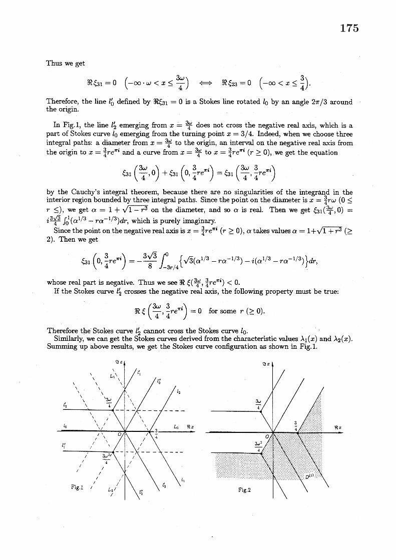
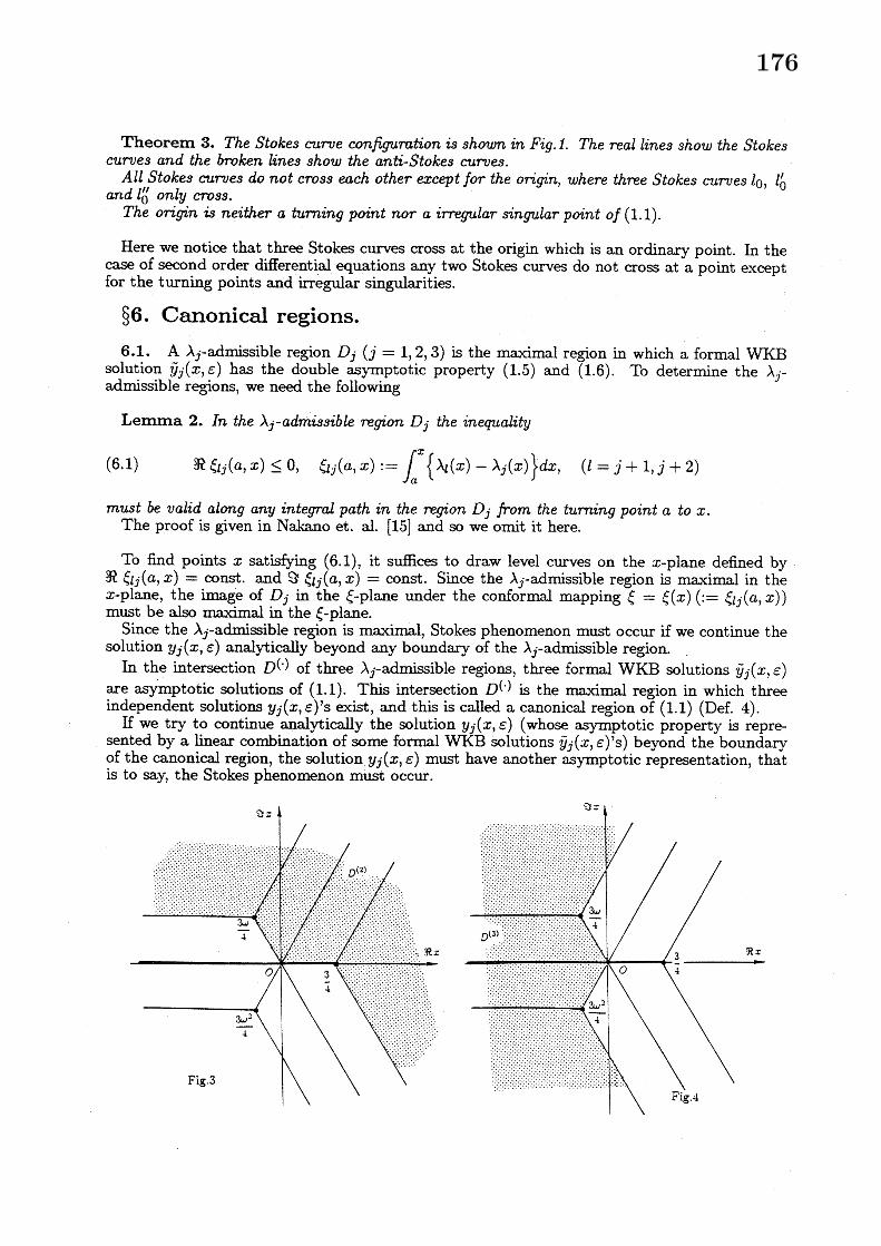
Thus we getTheorem 4. There nist three canonical regions $D^{(1)},$ $D(2)$ and $D^{(3)}$ of the $e\varphi_{4}abion(1.1)$ as

shovm in Fig.2\sim 4. They are situated symmetrically around the $07^{\cdot}i\dot{\varphi}n$, especially $D^{(2)}=\overline{D}^{(1)}$$:=$

$\{\overline{x}:x\in D^{()}1\}$ .

6.2. Berk et. al. [3] study the equation Ia with two simple tuming points and they assertthat the Stokes phenonenon occurs on the new Stokes curve, which $\mathrm{e}\mathrm{m}\mathrm{e}\mathrm{r}_{\mathrm{t}\supset}\sigma \mathrm{e}\mathrm{s}$ from the intersectionpoint (which is called a new turning point by Aoki et. al. [2]) of the ‘old’ Stokes curves, inorder to continue solutions by using Furry’s rule which was obtained for second order equationswith simple turning points.

But the equation Ib with three simple tuming points needs no new Stokes curves to constructcanonical regions (Theorem 4).

By the way, Berk et. al. state that there exist six directions of Stokes curves to $\infty \mathrm{e}\mathrm{m}\mathrm{e}\mathrm{r}_{\mathrm{o}}\sigma \mathrm{i}\mathrm{n}\mathrm{g}$

from two simple $\mathrm{t}\mathrm{u}\mathrm{r}\mathrm{n}\mathrm{i}\mathrm{n}_{\circ}\sigma$ points, although the local theory at an irregular singular point assertsthat there axist eight Stokes curves emerging from $\infty$ (Wasow [17]).

The equation Ib has nine Stokes curves emerging from three simple turning points and theytend to $\infty$ in three different directions, and the local theory at an $\mathrm{i}\mathrm{r}\mathrm{r}\mathrm{e}_{\mathrm{o}}\circ \mathrm{u}\mathrm{l}\mathrm{a}\mathrm{r}$ singular point assertsthat three Stokes curves emerge from $\infty$ (cf. $84.3$)$\mathit{0}^{\cdot}$

Now, we propese

Conjecture. Let $N_{t}$ be a number of directions of Stokes curves tending to $\infty eme\tau.\dot{\varphi}ng$ fromall the tuming points and let $N_{\infty}$ be a number of direcbons of Stokes curves emerging from $\infty$ .If $N_{t}=N_{\infty}$ , then there mist no new Stokes curues.

\S 7. Laplace transforms.7.1. As known well, a solution of a linear ordinary differential equation with linear $\mathrm{c}o$effi-

cients, which is called a Laplace equation, can be represented by the Laplace transform or theLaplace integral. The Laplace transform of (3.1) is

$y(x, \epsilon)$ $= \int_{\gamma}\frac{1}{-4s}\exp\{$

(7.1)

$=- \frac{1}{4}\int_{\gamma}\frac{1}{s^{1-1/}}$

$\frac{1}{\epsilon}(xs-\frac{s^{3}}{12}+\log s^{1/}2)\}\ \mathrm{s}$

$2 \epsilon\exp\{\frac{1}{\epsilon}(xs-\frac{s^{3}}{12}\mathrm{I}\}ds$ ,

if we suppose that the $\mathrm{i}\mathrm{n}\mathrm{t}\mathrm{e}_{\mathrm{o}\mathrm{o}}\sigma \mathrm{r}\mathrm{a}1\omega \mathrm{n}\mathrm{v}\mathrm{e}\mathrm{r}\sigma \mathrm{e}\mathrm{S}$.When we put $S(s, x):=xs-s^{3}/12+\log s^{1/}2$ , then $\partial S/\partial s=x-s^{2}/4+1/2s=-(s^{3}-4_{X}s-$

$2)/(4s)$ .Zeros of $\partial S/\partial s$ are called saddle points of the integral (7.1). The numerator $s^{3}-4Xs-2$ of

$\partial S/\partial s$ coincides with the characteristic polynomial of the equation (3.1), and its zeros are thecharacteristic values of (3.1). Thus we get

LEMMA 3. The characteriS$ti_{C}$ values of the equation (3.1) are $\mathit{8}addle$ point8 of (7.1).

When 8 is sufficiently large, the integral (7.1) must $\infty \mathrm{n}\mathrm{v}\mathrm{e}\mathrm{r}_{\circ}\sigma \mathrm{e}$. The convergence regions in the$s$-plane are derived from $Re(-s^{3}/12)<0$ . The $\mathrm{o}\mathrm{r}\mathrm{i}_{\circ}\sigma \mathrm{i}\mathrm{n}$ of the -plane is a singular point of theintegrand, but the integral converges at the $\mathrm{o}\mathrm{r}\mathrm{i}_{6}\sigma \mathrm{i}\mathrm{n}$ , because the exponent $1-1/2\epsilon(\epsilon>0)$ issmmller than 1.

7.2. If we choose the integral path $\gamma$ such that it passes through the saddle point andcomes from and goes to $\infty$ or from $0$ to $\infty$ in the convergence regions, we can get asymptoticrepresentations of the Laplace $\mathrm{i}\mathrm{n}\mathrm{t}\mathrm{e}_{\mathrm{o}}\sigma \mathrm{r}\mathrm{a}1$ by the saddle point method or the method of the steepestdescent as follows:

(7.2) $y(x, \epsilon)\sim C(\epsilon)\frac{\lambda^{1/2\epsilon}}{\sqrt{\lambda^{3}+1}}e^{\frac{1}{\epsilon}\frac{2}{3}}x\lambda$ ($\epsilonarrow 0,$ $xarrow\infty$ ; for any $\lambda$);

177

(7.3) $y_{j}(x, \epsilon)\sim\frac{x^{1/4\epsilon}}{\sqrt{\lambda_{\mathrm{j}}^{3}+1}}e(-1)^{\mathrm{t}}j+1)/2\underline{1}_{\frac{4}{3}}x/32\vdash\vee-(j=1,3),$ $y_{2}(_{X\epsilon},) \sim\frac{x^{-1/2\epsilon}}{\sqrt{\lambda_{2}^{3}+1}}(\epsilonarrow 0, xarrow\infty)$ .

Right hand sides of (7.3) are same as WKB solutions (1.4) if we calculate a root of (1.4) muchmore. After a short calculation we get more precise form from (7.3):

(7.4) $y_{1}(X, \epsilon)\sim Xe(1-3\zeta)/4\epsilon\frac{1}{r^{\underline{-}}}\frac{4}{3}x^{3}/2,$ $y_{2}(x, \epsilon)\sim x^{-}1/2_{\mathcal{E}},$ $y_{3}(x, \epsilon)\sim x-/4\epsilon e^{-}(13\epsilon)\frac{1}{\epsilon}\frac{4}{3}x3/2$

Thus we get

LEMMA 4. The Laplace transform $ha\mathit{8}$ the formal $WKB$ solutions as osymptotic $e\varphi ans\dot{f}on\mathit{8}$ .

\S 8. The Airy functions.8.1. Rom now on, we assume $\epsilon=1$ . Then the equation (3.1) becomes

(8.1) $y”’-4Xy’-2y=0$.

The Airy functions $\mathrm{A}\mathrm{i}(x)$ and $\mathrm{B}\mathrm{i}(x)$ are linearly independent solutions of the Airy equation

(3.2) $\mathrm{Y}’’-xY=0$ .

If we put $y:=Y^{2}$ , then $y$ satisfies (8.1), i.e., $Y^{2}$ is a solution of (8.1). More precisely speaking,$\mathrm{A}\mathrm{i}^{2},$ $\mathrm{A}\mathrm{i}\cdot \mathrm{B}\mathrm{i}$ and $\mathrm{B}\mathrm{i}^{2}$ are linearly independent solutions of (8.1). The wronskian of $\mathrm{A}\mathrm{i}^{2},$ $\mathrm{A}\mathrm{i}\cdot \mathrm{B}\mathrm{i}$ and$\mathrm{B}\mathrm{i}^{2}$ is $2\pi^{-3}$ .

Asymptotic properties of the Airy functions are: for $xarrow\infty$

(8.2) $\mathrm{B}\mathrm{i}(x)\sim\frac{1}{\sqrt{\pi}}x^{-1/4}e^{\frac{2}{3}x^{3}}/2$ $(| \arg x|<\frac{\pi}{3})$ , $\mathrm{A}\mathrm{i}(x)\sim\frac{1}{2\sqrt{\pi}}x^{-1/4-}e\frac{2}{3}x3/2$ $(|\arg x|<\pi)$ ,

then by making simply products we get

(8.3) $\{$

$\mathrm{B}\mathrm{i}(X)^{2}\sim\frac{1}{\pi}x^{-1/2}e^{\frac{4}{3}x^{3}}/2$ $(xarrow\infty,$ $| \mathrm{a}r\mathrm{g}x|<\frac{\pi}{3})$ ,

$\mathrm{A}\mathrm{i}(x)\cdot \mathrm{B}\mathrm{i}(x)\sim\frac{1}{2\pi}x^{-1/2}$ $(x arrow\infty, |\arg x|<\frac{\pi}{3})$ ,

$\mathrm{A}\mathrm{i}(X)^{2}\sim\frac{1}{4\pi}x^{-1/2-}e\frac{4}{3}x3/2$ $(xarrow\infty,$ $|\arg x|<\pi)$ .

Right hand sides of (8.3) are formal WKB solutions of (8.1) corresponding to the characteristicvalues $\lambda_{1}(x),$ $\lambda_{2}(x)$ and $\lambda_{3}(x)$ in order. Thus, (8.3) coincides with (7.4) when $\epsilon=1$ if we takeno account of constants.

8.2. Between two Airy functions $\mathrm{A}\mathrm{i}(x)$ and $\mathrm{B}\mathrm{i}(x)$ there is a linear relation (Abranowitz-Stegun [1] $)$

(8.4) $2\mathrm{A}\mathrm{i}(xe^{\pm 2\pi}i/3)=e^{\pm\pi i/}\{3\mathrm{A}\mathrm{i}(X)\mp i\mathrm{B}\mathrm{i}(x)\}$.By squaring this we get the relation

(8.5) $4\mathrm{A}\mathrm{i}(xe^{\pm 2}\pi i/\mathrm{s})2=e^{\pm 2\pi i/3}\{\mathrm{A}\mathrm{i}(X)^{2}\mp 2i\mathrm{A}\mathrm{i}(x)\mathrm{B}\mathrm{i}(x)-\mathrm{B}\mathrm{i}(x)^{2}\}$.This equation $\infty \mathrm{n}\mathrm{t}\mathrm{a}\dot{\mathrm{m}}\mathrm{s}$ four functions which are solutions of (8.1). Therefore, (8.5) represents alinear relation between four solutions of (8.1) and it is a connection formula. The asymptoticproperty (8.2) and the relation (8.4) are gained from the Laplace $\mathrm{i}\mathrm{n}\mathrm{t}\mathrm{e}_{\mathrm{o}}\sigma \mathrm{r}\mathrm{a}1$ for the Airy equation:

(8.6) $Y= \frac{1}{2\pi i}\int_{\gamma}e^{tx-t}’ d3t3/$ .

178

The Laplace integral for $(8.1)$,

is got from (7.1) by putting $\epsilon=1$ and it is

(8.7) $y– \int_{\gamma}\frac{1}{\sqrt{s}}e^{xS-}ds^{3}/12S$ .

We must notice that (8.5) is not got from (8.7) but simply got by making a product of (8.4).

\S 9. Products of the Airy functions.

9.1. By formal calculation, we see that a product of (8.6) becomes (8.7):

(9.1) $( \int e^{tx-i^{\mathit{3}}/3)}.dt2=\mathrm{c}\mathrm{o}\mathrm{n}\mathrm{S}\mathrm{t}.\int\frac{1}{\sqrt{s}}e^{xs-S^{3}}d_{\mathit{8}}/12$.

The Airy functions $\mathrm{A}\mathrm{i}(x)$ and $\mathrm{B}\mathrm{i}(x)$ are composed of three parts, $I_{1}(x),$ $I_{2}(x)$ and $I_{3}(x)$ , as$\mathrm{f}o$llows (Jeffieys-Jeffieys [11]):

(9.2) $\mathrm{A}\mathrm{i}(x)=I_{2}(x)-I_{3(}x)$ , $\mathrm{B}\mathrm{i}(x)=i\{2I_{1}(x)-I_{2}(X)-I_{3}(x)\}$ ,

where $I_{j}(x)’ \mathrm{s}$ are defined by the Laplace $\mathrm{i}\mathrm{n}\mathrm{t}\mathrm{e}_{\mathrm{o}^{\mathrm{T}\mathrm{a}}}\circ 1$ of the Airy equation:

(9.3) $\{$

$I_{1}(x):= \frac{1}{2\pi i}\int_{0}^{+\infty}e^{tx-t}d/3t3$ ,

$I_{2}(x):= \frac{1}{2\pi i}\int_{0}^{\mathrm{K}}e^{t}-t/3dxt3$ ,

$I_{3}(x):= \frac{1}{2\pi i}\int_{0}^{\propto\omega^{2}}e^{r\prime x-}d3ti\mathit{3}/$ .

Here we must notice that $I_{2}(x)-I_{3}(x)$ and 2 $I_{1}(x)-I_{2}(x)-I_{3}(x)$ are solutions of the Airyequation (3.2), but each of $I_{j}(X)_{\mathrm{S}}$

’ is not a $\infty \mathrm{l}\mathrm{u}\mathrm{t}\mathrm{i}\mathrm{o}\mathrm{n}$ of the $\mathrm{A}\dot{\eta}$ equation (8.6).Then, by squaring (9.2) or making a product of them, we get

(9.4) $\{$

$\mathrm{A}\mathrm{i}^{2}=I_{2}^{2}-2I_{2}I_{3}+I_{3}^{2}$ ,$\mathrm{A}\mathrm{i}\cdot \mathrm{B}\mathrm{i}=i(2I_{1}I_{2}-I^{2}2-2I_{1}I_{3}+I_{3}^{2})$ ,$\mathrm{B}\mathrm{i}^{2}=-4I_{1}2-I_{2^{-I^{2}}}23+4I_{1}$ I2–2$I_{2}I_{3}$ .

From (9.1) and (9.3), we want to expect the following relations

(9.5) $I_{1}^{2}= \int_{0}+\infty d_{\mathit{8}}\frac{1}{\sqrt{\sim^{\mathrm{q}}}}exs-S3/12$, $I_{2}^{2}=I_{0} \infty\omega\frac{1}{\sqrt{s}}exs-S^{3}/12ds$ , $I_{3}^{2}= \int_{0}\mathrm{w}^{2}\frac{1}{\sqrt{s}}e-s/312dxs\mathit{8}$.

However, the relations (9.5) are not vahid.

9.2. The right hand sides of (9.4) are too complicated to define solutions of (8.1). $\mathrm{A}\mathrm{i}(x)$ ,$\mathrm{A}\mathrm{i}(\omega x),$ $\mathrm{A}\mathrm{i}(\omega^{2}x),$ $\mathrm{B}\mathrm{i}(x),$ $\mathrm{B}\mathrm{i}(\omega X)$ and $\mathrm{B}\mathrm{i}(\omega^{2}x)$ are solutions of the Airy equation, and $\mathrm{A}\mathrm{i}(X)^{2}$ ,$\mathrm{A}\mathrm{i}(\omega x)^{2},$ $\mathrm{A}\mathrm{i}(\omega x2)^{2}$ and other products of them are solutions of (8.1), but we adopt more simplythe right hand sides of (9.5) as the standard solutions of (8.1) and denote them by

(9.6) $\{$

$\mathrm{A}\mathrm{p}(_{X}):=\int_{0}^{+\infty}\frac{1}{\sqrt{s}}e^{xs}-s/312dS$,

$\mathrm{B}\mathrm{p}(X,):=\Gamma^{\frac{1}{\sqrt{s}}}\mathrm{o}e^{xS}-s^{3}/12dS$,

$\mathrm{C}\mathrm{p}(_{X}):=\int_{0}^{\infty\omega^{2}}\frac{1}{\sqrt{s}}e^{xs-}ds/312S$.

179

From (9.6), we see that

(9.7) $\mathrm{A}\mathrm{p}(xe2\pi\dot{l})=\mathrm{A}\mathrm{p}(x)$ , $\mathrm{B}\mathrm{p}(xe^{2\pi i})=\mathrm{B}\mathrm{p}(x)$ , $\mathrm{C}\mathrm{p}(Xe2\pi i)=\mathrm{C}\mathrm{p}(X)$

are vahid. Therefore $\mathrm{A}\mathrm{p}(x),$ $\mathrm{B}\mathrm{p}(x)$ and $\mathrm{C}\mathrm{p}(X)$ are single-valued and entire functions.Three functions Ap, Bp and Cp are defined by independent integral paths, then they are

linearly independent solutions of (8.1) and all other solutions of (8.1) can be represented by alinear combination of Ap, Bp and Cp.

Summing up we get

Thorem 6. Three $fi_{4nCt}i_{onS}\mathrm{A}\mathrm{P}(X),$ $\mathrm{B}\mathrm{p}(x)$ and $\mathrm{C}\mathrm{p}(X)$ defined by (9.6) are not created fromparts $I_{j}(x)fs$ of the $Ai\eta$ functions (see (9.2)). They are linearly independent solutions of (8.1)and srngle-valued entire functions. The $7\dot{\mathrm{z}}ght$ hand sides of (7.4) becomes the formal $WKB$ solu-tions of (8.1) by putting $\epsilon=1$ .

In Zwillinger [21] the equation (8.1) is cited but it has no name, and so we propose hereto name the equation (8.1) the Pairy equation and three functions Ap, Bp and Cp Pairyfunctions. The name ‘Pairy’ is originated from Pairy$=(\mathrm{P}\mathrm{r}o\mathrm{d}\mathrm{u}\mathrm{C}\mathrm{t}\mathrm{s}+Airy)/2$.

REFERENCES[1] Abranowitz, M., and I.A. Stegun, Handbook of mathematical functions, Dover.[2] Aoki,T., Kawai, T. and Y. Takei, New turning points in the exact $\mathrm{W}^{7}\mathrm{K}\mathrm{B}$ analysis for higher-order

ordinary differential equations. RIMS Dec., 1991, 1-16.$23.\mathrm{b}_{88}[3\mathrm{B}\mathrm{e}- \mathrm{r}_{1}\mathrm{k},\mathrm{H}00^{\underline{9}},\cdot 1\mathrm{L},\mathrm{W}9\dot{8}2$

.. M. Nevins and K. V. Roberts, New Stokes line in WKB theory. J. Math. Phys.

[4] Briuouin, L., Remarques sur la m\’echanique ondulatoire. J. Phys. Radium [6], 7, 353-368, 1926.[51 Evgrafov, M. A., and M. V. Fedoryuk, Asymptotic behavior as ノ\\rightarrow \infty of solutions of the equation

$w”1- 4\S^{\sim}’,)_{1^{-\ovalbox{\tt\small REJECT}^{(Z}’)}}.\lambda)9w(z=0$in the $\mathrm{c}\mathrm{o}\mathrm{m}\mathrm{p}\mathrm{l}\infty z$-plane. Uspehi Mat. Nauk 21, or Russian Math. Surveys 21,

[6] Fedoryuk, M. V., The topology of Stokes lines for equations of the second order. A. M. S. Transl.(2) 89. 89-102, 1970, or Izv. Akad. Nauk SSSR Ser. Mat. 29, 645-656, 1965.

[7] Fedoryuk, M.V., Asymptotic properties of the solutions of ordinary n-th order linear differentialequations. Diff. Urav. 2, 492-507, 1966.

[8] $\mathrm{F}\mathrm{e}\mathrm{d}_{\mathrm{o}\mathrm{r}\}}\eta 1\mathrm{k},$ M, V., The encyclopaedia of mathematical sciences. 13, Analysis I, 84-191, 1986.[9] Fedoryuk, M. V., Asymptotic Analysis, Springer Verlag. 1993.[10] Fukuhara, M., Sur les proprietes asymptotiques des solutions d’un systeme d’equations differen-

tielles lin\’eaires contenant un parametre. Mem. Fac. Engrg., Kyushu Imp. Univ. 8, 249-280, 1937.[11] Jeffreys, H., and B. S. Jeffreys, Methods of mathematical physics. Cambridge Univ Press, 1956.

$60,2\iota^{\mathrm{K}\mathrm{e}}[1241-\underline{\circ}l_{1}\mathrm{u},’ \mathrm{B}\mathrm{J}\dot{9}79.\cdot$

, Admissible domains for higher order differential equations. Studies in Appl. Math.

[13] Kramers, H. A., Wellennechanik und halbzahlige Quantisierung. Z. Physik 39, 823840, 1926.. [14] Nakano, M., On products of the Airy functions and the WKB method, J. of Tech. Univ. atPlovdiv. 1, 27-38, 1995.

[15] Nakano, M., M. Namiki and T. Nishimoto, On the WKB method for certain third order ordinarydifferential equations, Kodai Math. J. 14. 432-462,1991.

[16] Olver, F. W. J., Asymptotics and special functions. Academic Press, 1974.[17] Tumittin, H. L., Asymptotic exxppansions of solutions of systems of ordinary differential equations,

Contributions to the Theory of Nonlinear Oscillations II. Ann. of Math. Studies 29, 81-116, Princeton,1952.

[18] Wasow, W., Asymptotic expansions for ordinary differential equations. Wiley (Interscience), 1965.$\mathrm{t}1,\mathrm{G}.,\mathrm{E}\mathrm{i}\mathrm{n}\mathrm{e}\mathrm{n}\mathrm{e}\mathrm{a}r\mathrm{t}\mathrm{u}\mathrm{r}\mathrm{n}\mathrm{i}\mathrm{v}_{\mathrm{e}}\mathrm{r}\mathrm{a}\mathrm{u}_{\mathrm{g}}\mathrm{e}\mathrm{m}\mathrm{e}\mathrm{i}^{\circ \mathrm{i}\mathrm{n}}\mathrm{n}\mathrm{e}\mathrm{r}\mathrm{u}\mathrm{n}\mathrm{g}\mathrm{d}\mathrm{n}\mathrm{g}\mathrm{p}\mathrm{t}\mathrm{t}\mathrm{h}\infty \mathrm{r}\mathrm{y}\mathrm{e}\mathrm{r}\mathrm{Q}\mathrm{u}\mathrm{a}\mathrm{n}\mathrm{t}\mathrm{e}\mathrm{n}\mathrm{b}\mathrm{e}\mathrm{d}\dot{\mathrm{m}}\mathrm{g}\mathrm{u}\mathrm{n}_{\mathrm{o}}\sigma \mathrm{e}\mathrm{n}\mathrm{f}\mathrm{i}\dot{\mathrm{m}}\mathrm{S}\mathrm{p}\mathrm{r}\mathrm{i}\mathrm{n}\mathrm{g}\mathrm{e}\mathrm{r}\mathrm{V}\mathrm{e}\mathrm{r}1\mathrm{a}\mathrm{g},1985$

die Zwecke der Wellenmechnik.Z.Physik 38, 518-529, 1926.

[21] Zwilhnger, D., Handbook of differential equations. $\mathrm{A}_{\mathrm{C}\mathrm{a}}\mathrm{d}\mathrm{e}\mathrm{m}\mathrm{i}\mathrm{C}$ Press, 1989.

180