Embed Size (px)
Citation preview
On the Lagrangian Theory of Structure Formation in
Relativistic Cosmology : intrinsic Perturbation
Approach and Gravitoelectromagnetism
Fosca Al Roumi
To cite this version:
Fosca Al Roumi. On the Lagrangian Theory of Structure Formation in Relativistic Cosmology :intrinsic Perturbation Approach and Gravitoelectromagnetism. Cosmology and Extra-GalacticAstrophysics [astro-ph.CO]. Universite Claude Bernard - Lyon I, 2015. English. <NNT :2015LYO10136>. <tel-01367703>
HAL Id: tel-01367703
https://tel.archives-ouvertes.fr/tel-01367703
Submitted on 16 Sep 2016
HAL is a multi-disciplinary open accessarchive for the deposit and dissemination of sci-entific research documents, whether they are pub-lished or not. The documents may come fromteaching and research institutions in France orabroad, or from public or private research centers.
L’archive ouverte pluridisciplinaire HAL, estdestinee au depot et a la diffusion de documentsscientifiques de niveau recherche, publies ou non,emanant des etablissements d’enseignement et derecherche francais ou etrangers, des laboratoirespublics ou prives.
Thèseprésentée devant
l’Université Claude Bernard Lyon - I
École Doctorale de Physique et d’Astrophysiquepour l’obtention du
DIPLÔME de DOCTORAT
Spécialité : Physique Théorique / Cosmologie
(arrêté du 7 août 2006)
par
Fosca Al Roumi
Théorie Lagrangienne Relativiste dela Formation des Grandes Structures :
Description Intrinsèque des Perturbationset Gravitoélectromagnétisme
A soutenir publiquement le 18 Septembre 2015 devant la Commission d’Examen :
Prof. P. Salati Président du jury - LAPTH, Annecy le VieuxProf. B. Roukema Rapporteur et examinateur - Torún Centre for Astronomy, TorúnProf. R. Sussman Rapporteur et examinateur - Instituto de Ciencias Nucleares, México, D. F.Prof. R. Triay Examinateur - CPT, MarseilleProf. R. Walder Examinateur - CRAL, LyonProf. T. Buchert Directeur de thèse - CRAL, Lyon

PHD THESIS of the UNIVERSITY of LYON
Delivered by the UNIVERSITY CLAUDE BERNARD LYON 1
Subject:
THEORETICAL PHYSICS / COSMOLOGY
submitted by
Ms FOSCA AL ROUMI
for the degree of
DOCTOR OF THEORETICAL PHYSICS
On the Lagrangian Theory ofStructure Formation in Relativistic Cosmology:
Intrinsic Perturbation Approachand Gravitoelectromagnetism
To be defended 18 September 2015 in front of the following ExaminingCommittee:
Prof. P. Salati President - LAPTH, Annecy le VieuxProf. B. Roukema Reviewer and examiner - Torún Centre for Astronomy, TorúnProf. R. Sussman Reviewer and examiner - Instituto de Ciencias Nucleares, Mexico CityProf. R. Triay Examiner - CPT, MarseilleProf. R. Walder Examiner - CRAL, LyonProf. T. Buchert Supervisor - CRAL, Lyon

Acknowlegments / Remerciements
First of all I would like to thank my mentor, Thomas Buchert. It will take me manyyears to realize how lucky I’ve been to work under your direction. Thank you for all yourscientific skills, your patience and your rigor. But most of all, thank you for your sense ofhumor, your creativity and for being so open-minded. I hope I took some of your qualitiesduring these three years.
I wish to thank Gilles Chabrier for his fruitful remarks during seminars and for hostingus at CRAL-ENS.
My thanks to Herbert Wagner and Martin Kerscher, with whom I worked in Munichon gravitoelectromagnetism. Your help, remarks and advices have been very importantfor my work on this topic. This student exchange was supported by the French–BavarianCooperation Center, BFHZ Munich http://www.bayern-france.org/.
Special thanks to Xavier Roy, who helped me a lot throughout the PhD. Thank youfor the detailed answers to my questions, for all the explanations on foliation of space-timeand differential geometry and for all the useful advices you gave me on the manuscript.Thank you also for all the non-scientific discussions we had. They have been crucial tome.
My thanks to Alexander Wiegand for the fruitful discussions, the nice work we didtogether, for you time and advices.
Thanks to Léo Brunswic for all the work we achieved on topology and Hodge decom-position. Your mathematical skills have been really precious for this work.
I wish also to thank Alexandre Alles for the help and the useful discussions on theblackboard.
My thanks to Boud Roukema for the useful discussions on topology and for his veryinteresting work on inhomogeneous cosmology. Thank you for your time and help!
Thanks to Frank Steiner for sharing his great knowledge on cosmic topology.Martin France, thank you for all the nice discussions we had on the CMB.Thanks to Rolf Walder for the nice remarks and discussions we had during the semi-
nars.I would also like to thank Roberto Sussman and Boud Roukema for having accepted
to be reviewer of my thesis and spending some of your precious time on reading my thesisand writing a report.
I also want to thank Pierre Salati for being the president of my examining committee,for the very interesting discussions we had on the scalar model for dark matter at thebeginning of my PhD and at Cargèse last september. Thank you also for all the help gaveme in my research career.
iii
I also want to thank Roland Triay and Rolf Walder for having accepted to be examinerof my thesis.
Thanks to Jan Ostrowski for everything: from physics to beers and ping-pong.Thanks also to Pierre Mourier for the scientific discussions and the nice time we had
together. Good luck with your PhD!Thanks to Thomas Buchert, Martin France, Boud Roukema, Rolf Walder, Frank
Steiner, Léo Brunswick, Jan Ostrowski, Tomek Kazimierczak and Pierre Mourier for thereally nice dinners we had together. It is a pleasure to talk about science or somethingelse around a glass of wine!
Je voudrais aussi remercier Stephanie Vignier, Sylvie Réa and Sylvie Flores pour avoirrendu tous les aspects administratifs bien plus simples. C’est toujours avec grand plaisirque je suis allée vous poser des questions et vous demander de l’aide. Merci pour votrepatience et votre bonne humeur!
Vielen Dank an Marie von München. Les quelques jours de rédaction à Munich ontétés un vrai plaisir!
Merci à tous mes amis lyonnais, qui m’ont fait passer d’excellents moments pendantces trois ans! Merci à Julien, Catherine, Martin, Elisa, Tatjana, Camille, Grégoire, Lila,Elsa, Thiago, Mariana, Mirella et Matei.
Un grand merci à mes colocs adorés, Matteo et Lucy. Quel bonheur d’avoir partagéavec vous le même toit!
Martin, merci aussi pour tous tes conseils sur la rédaction de la thèse! Tatjana, mercide m’avoir acceuillie après cette longue période de rédaction à Milano, la ville qui nese couche jamais. Julien, merci de m’avoir aidée à certains moments particulièrementdélicats!
Merci aussi à mes amis parisiens! Julia, Fanny et Victoria, les moments que nousavons passés ensemble et les fous rires que nous avons eus ont grandement participé àmon équilibre mental. Merci aussi à Daniel, Louison, Olivier, Léo. J’espère vous voir plussouvent maintenant.
Merci enfin à Mohamad et Amélie pour avoir toujours étés là pour moi. Vous m’avezbeaucoup aidée. Merci aussi à mon frère Meyar pour m’avoir prêté son coffret Paradjanov.Constance, il faudrait un chapitre entier pour te remercier. Alors, je préfère le faire devive voix dans un bon restaurant!
Sans ces rencontres et ces échanges, mon travail de thèse n’aurait pas été possible. Jevous remercie donc sincèrement.
iv
Abstract
The dynamics of structure formation in the Universe is usually described by Newto-nian numerical simulations and analytical models in the frame of the Standard Model ofCosmology. The structures are then defined on a homogeneous and isotropic background.Such a description has major drawbacks since, to be self-consistent, it entails a largeamount of dark components in the content of the Universe.
Different strategies are considered to solve this enigma. Particle physicists have beensearching for some exotic sources of the stress-energy tensor to account for these darkcomponents. Nevertheless, no direct evidence of these 26% of dark matter and 69% ofdark energy has yet been given. Therefore, some alternative theories to General Relativityare explored.
To address the problem of dark matter and dark energy, we will neither supposethat exotic sources contribute to the content of the Universe, nor that General Rela-tivity is obsolete. We will develop a more realistic description of structure formation inthe frame of General Relativity and thus no longer assume that the average model isa homogeneous-isotropic solution of the Einstein equations, as claimed by the StandardModel of Cosmology.
During my work under the supervision of Thomas Buchert, I contributed to the devel-opment of the perturbative formalism that enables a more realistic description of space-time dynamics. In the framework of the intrinsic Lagrangian approach, which avoids defin-ing physical quantities on a flat background, I contributed to the building of relativisticsolutions to the gravitoelectric part of the Einstein equations from the generalization ofthe Newtonian perturbative solutions. Moreover, the gravitoelectromagnetic approach Iworked with has provided a new understanding of the dynamics of the analytical solu-tions to the field equations. Finally, treating globally the spatial manifold, I used powerfulmathematical tools and theorems to describe the impact of topology on the dynamics ofgravitational waves.
v

Résumé
La dynamique de formation des structures de l’Univers est habituellement décrite dansle cadre du modèle standard de Cosmologie par des simulations numériques newtonienneset des modèles analytiques. Les structures sont alors associées à des grandeurs définiessur un fond homogène et isotrope. Cependant, pour que les observations cosmologiquessoient cohérentes avec le modèle standard, il est nécessaire de supposer l’existance d’unegrande proportion d’éléments de nature inconnue dans le contenu de l’Univers.
Différentes stratégies sont envisagées pour déterminer la nature de ces éléments. Eneffet, les physiciens des particules cherchent des particules exotiques, qui pourraient alorsrendre compte des 26% de matière noire et 69% d’énergie sombre. Cependant, aucunemesure expérimentale n’ayant pour l’instant démontré l’existence de ces éléments, desthéories de gravitation alternatives à la relativité générale sont actuellement envisagées.
Pour tenter de résoudre ce problème, nous ne considèrerons pas d’autres sources dansle contenu de l’Univers que celles ordinaires et resterons dans le cadre de la RelativitéGénérale. Nous développerons néanmoins une description plus réaliste de la formation destructures dans le cadre de la théorie d’Einstein. Ainsi, contrairement au modèle standardde Cosmologie, nous ne supposerons pas que l’Univers moyenné est une solution homogèneet isotrope des équations d’Einstein.
Lors de mon travail sous la direction de Thomas Buchert, j’ai participé au développe-ment d’un formalisme perturbatif permettant une description plus réaliste de la dy-namique de l’espace-temps. J’ai également contribué à l’obtention de solutions relativistesà la partie gravitoélectrique des équations d’Einstein en généralisant les solutions per-turbatives newtoniennes. Ces travaux ont été réalisés dans le cadre d’une approche la-grangienne intrinsèque, évitant ainsi de définir les grandeurs physiques sur un fond plat.L’approche gravitoélectromagnétique que j’ai adoptée m’a permis une interprétation nou-velle et performante des solutions des équations d’Einstein. Enfin, j’ai étudié l’impact dela topologie sur la dynamique des ondes gravitationelles à l’aide d’une description globalede l’hypersurface spatiale, permise par des théorèmes mathématiques puissants.
vii


“Put your hand on a hot stove for a minute,and it seems like an hour.
Sit with a pretty girl for an hour,and it seems like a minute.
That’s relativity!”
Albert Einstein

Contents
Motivation 1
I Introduction 5
1 General Relativity and the Standard Model of Cosmology 71.1 Einstein’s theory of General Relativity . . . . . . . . . . . . . . . . . . . . 8
1.1.1 From Newtonian gravity to General Relativity . . . . . . . . . . . . 91.1.2 Einstein’s field equations . . . . . . . . . . . . . . . . . . . . . . . . 11
1.2 Homogeneous and Isotropic Cosmology . . . . . . . . . . . . . . . . . . . . 121.2.1 The Cosmological Principle and the Hubble law . . . . . . . . . . . 121.2.2 Homogeneous and isotropic universe models . . . . . . . . . . . . . 13
1.3 Standard model of Cosmology and structure formation . . . . . . . . . . . 161.3.1 Early stages . . . . . . . . . . . . . . . . . . . . . . . . . . . . . . . 161.3.2 Decoupling and the CMB anisotropies . . . . . . . . . . . . . . . . 19
2 Large Scale Structure Formation 212.1 Vlasov equation and Newtonian Eulerian dynamics . . . . . . . . . . . . . 22
2.1.1 The Vlasov-Newton system . . . . . . . . . . . . . . . . . . . . . . 222.1.2 Structure formation, shell-crossing and velocity dispersion . . . . . 252.1.3 Eulerian perturbation scheme . . . . . . . . . . . . . . . . . . . . . 262.1.4 Numerical simulations . . . . . . . . . . . . . . . . . . . . . . . . . 27
2.2 Newtonian Lagrangian perturbation approach to describe structure formation 282.2.1 Lagrangian description of structure formation . . . . . . . . . . . . 292.2.2 Lagrange-Newton System . . . . . . . . . . . . . . . . . . . . . . . 302.2.3 Zel’dovich approximation . . . . . . . . . . . . . . . . . . . . . . . . 302.2.4 Newtonian Lagrangian perturbation theory . . . . . . . . . . . . . . 30
2.3 Relativistic Lagrangian description of structure formation . . . . . . . . . . 312.3.1 Cartan formalism and the dynamics of space-time . . . . . . . . . . 322.3.2 3 + 1 foliation of space-time in a Lagrangian approach . . . . . . . 34
3 Inhomogeneous Cosmology 373.1 Inhomogeneities and their consequences on the global dynamics . . . . . . 38
3.1.1 Hierarchical structures and their density contrast . . . . . . . . . . 383.1.2 A first insight into averaging and backreaction . . . . . . . . . . . . 39
3.2 Backreaction and spatial average of the Einstein equations . . . . . . . . . 39
3.2.1 Einstein equations in the 3 + 1 formalism . . . . . . . . . . . . . . . 403.2.2 Dynamics of a compact domain from the averaged Einstein equations 41
3.3 Can backreaction replace Dark Matter and Dark Energy? . . . . . . . . . . 43
II Insight into General Relativity via ElectromagnetismAnalogy 44
1 Gravitoelectromagnetism and Gravitoelectric Part of the EinsteinEquations 461.1 Preparatory remarks: 3 + 1 decomposition of the Einstein equations . . . . 48
1.1.1 Description of the fluid flow and foliation of space-time . . . . . . . 481.1.2 Lagrangian descriptions . . . . . . . . . . . . . . . . . . . . . . . . 521.1.3 3 + 1 decomposition of the Einstein equations . . . . . . . . . . . . 531.1.4 Lagrangian formulation of Einstein’s equations for an irrotational
dust fluid matter model . . . . . . . . . . . . . . . . . . . . . . . . 541.2 Historical introduction to GEM . . . . . . . . . . . . . . . . . . . . . . . . 571.3 Maxwellian formulation of the Euler-Newton-System . . . . . . . . . . . . 581.4 Decomposition of the Weyl tensor and Maxwell-Weyl equations . . . . . . 61
1.4.1 Newtonian dynamics, tidal tensor and relativistic generalization . . 611.4.2 Electric and magnetic parts of the Weyl tensor . . . . . . . . . . . . 621.4.3 Maxwell-Weyl equations . . . . . . . . . . . . . . . . . . . . . . . . 631.4.4 Newtonian limit of the electric and magnetic parts . . . . . . . . . 65
1.5 Gravitoelectric part of the Einstein equations and the L-N-S . . . . . . . . 661.5.1 Gravitoelectric part of the Einstein equations . . . . . . . . . . . . 661.5.2 Minkowski Restriction of the gravitoelectric system . . . . . . . . . 671.5.3 Minkowski Restriction of the other Einstein equations . . . . . . . . 69
1.6 Concluding remarks . . . . . . . . . . . . . . . . . . . . . . . . . . . . . . . 70
2 Gravitoelectric Perturbation and Solution Schemes at Any Order 722.1 Construction schemes for relativistic perturbations and solutions . . . . . 75
2.1.1 General n–th order perturbation scheme . . . . . . . . . . . . . . . 752.1.2 Initial data for the perturbation scheme . . . . . . . . . . . . . . . 762.1.3 Gravitoelectric perturbation scheme . . . . . . . . . . . . . . . . . . 792.1.4 Gravitoelectric solution scheme . . . . . . . . . . . . . . . . . . . . 83
2.2 Application of the solution scheme . . . . . . . . . . . . . . . . . . . . . . 842.2.1 Systematics of the solutions . . . . . . . . . . . . . . . . . . . . . . 842.2.2 Reconstruction of the relativistic solutions . . . . . . . . . . . . . . 852.2.3 Example 1: recovering parts of the general first–order solution . . . 862.2.4 Example 2: constructing second–order solutions for ‘slaved initial
data’ . . . . . . . . . . . . . . . . . . . . . . . . . . . . . . . . . . . 892.3 Summary and concluding remarks . . . . . . . . . . . . . . . . . . . . . . . 91
III From a Local to a Global Description of First-OrderIntrinsic Lagrangian Perturbations 92
1 Gravitational Waves in the Standard Perturbation Theory 941.1 Propagative dynamics in the intrinsic approach: motivations and strategy . 951.2 Standard description of gravitational waves . . . . . . . . . . . . . . . . . . 96
1.2.1 Observing gravitational waves in the Standard Perturbation Theory 961.2.2 Linearizing the Einstein equations . . . . . . . . . . . . . . . . . . . 961.2.3 Gravitoelectromagnetism in the weak field limit . . . . . . . . . . . 981.2.4 Plane gravitational waves and polarization . . . . . . . . . . . . . . 98
2 Local Approach to First-Order Solutions 1002.1 Local approach and propagative dynamics . . . . . . . . . . . . . . . . . . 1012.2 First–order perturbation scheme in a local approach . . . . . . . . . . . . . 102
2.2.1 First–order perturbation scheme . . . . . . . . . . . . . . . . . . . . 1022.2.2 First–order equations . . . . . . . . . . . . . . . . . . . . . . . . . . 1032.2.3 First–order master equations . . . . . . . . . . . . . . . . . . . . . . 105
2.3 Electric and magnetic spatial parts of the Weyl tensor and the Maxwell-Weyl equations . . . . . . . . . . . . . . . . . . . . . . . . . . . . . . . . . 1072.3.1 Link to the electric and magnetic part of Weyl tensor . . . . . . . . 107
2.4 Comparison with the other perturbation schemes . . . . . . . . . . . . . . 1082.4.1 Non–propagating solutions for the intrinsic Lagrangian description . 1082.4.2 Propagative behavior of the non–integrable part . . . . . . . . . . . 1092.4.3 Comparison to other perturbation schemes . . . . . . . . . . . . . . 110
2.5 Conclusions and limits of the local description . . . . . . . . . . . . . . . . 113
3 Topology and Hodge Decomposition: a Global Approach to First-orderSolutions 1153.1 Introduction to the topology of the Cosmos . . . . . . . . . . . . . . . . . 116
3.1.1 Why are we interested in topology? . . . . . . . . . . . . . . . . . . 1163.1.2 Cosmic topology: from Einstein to recent times . . . . . . . . . . . 1173.1.3 Observational evidence for multiconnected spaces? . . . . . . . . . . 118
3.2 The Hodge decomposition and the first–order solutions . . . . . . . . . . . 1193.2.1 Thurston’s geometrization conjecture . . . . . . . . . . . . . . . . . 1193.2.2 Mathematical tools for the Hodge decomposition . . . . . . . . . . 1193.2.3 Hodge theorem . . . . . . . . . . . . . . . . . . . . . . . . . . . . . 1213.2.4 Hodge decomposition of the perturbation fields . . . . . . . . . . . 1223.2.5 Hodge decomposition of Cartan coframes for S3 topologies . . . . . 1233.2.6 From SVT to Hodge decomposition . . . . . . . . . . . . . . . . . . 124
3.3 Conclusions . . . . . . . . . . . . . . . . . . . . . . . . . . . . . . . . . . . 125
Conclusion & Outlook 127
A Lagrangian Perturbation Theory for Perfect Fluids in the Strong La-grangian Description 130A.1 Perfect fluid thermodynamics in the Strong Lagrangian description . . . . 131
A.1.1 Matter models . . . . . . . . . . . . . . . . . . . . . . . . . . . . . . 131A.1.2 Thermodynamics of the perfect fluid . . . . . . . . . . . . . . . . . 131A.1.3 Stress-energy tensor conservation and shift vector . . . . . . . . . . 132
A.2 First-order scheme for a radiation fluid . . . . . . . . . . . . . . . . . . . . 133A.2.1 First–order shift vector for a radiation fluid . . . . . . . . . . . . . 133A.2.2 Zero and first–order Einstein equations . . . . . . . . . . . . . . . . 134
A.3 Concluding remarks . . . . . . . . . . . . . . . . . . . . . . . . . . . . . . . 136
Motivation
Determining the nature of what surrounds us and its history has been one of themost ambitious project that human kind has dared to undertake. Through time, theprecision of the observations of the Universe has improved. Combined with philosophicaland theoretical developments, they led to changes of paradigms which finally resulted inour current idea of the Universe. The representation of the Universe shared by most ofthe observational cosmologists is the Standard Model of Cosmology, namely the ΛCDMmodel (Cold Dark Matter model with a cosmological constant modeling dark energy).This model gives the evolution of the Universe and its constituents, from the inflation tothe formation of large scale structures, and assumes a decoupling of the dynamics of thesmall structures with respect to the global evolution of space-time, which is described asbeing locally isotropic and hence homogeneous on all scales.
For the cosmological observations to be consistent with this model, a large amount ofunknown constituents has to be postulated. Indeed, at most 5% of the energy budget ofthe Universe can be explained using the matter content of the standard particle physicswhile ∼ 69% of the content of the Universe is attributed to dark energy and 26% to darkmatter, which are both of hypothetical origin.
Different strategies are considered to determine the true nature of these dark compo-nents. Particle physicists have been searching for some exotic sources of the stress-energytensor in order to account for these dark components. Even if many candidates for darkmatter and dark energy have been considered, no direct evidence has yet been obtained.Doubting of the success of the detection experiments undertaken by astroparticle physi-cists, alternative theories to General Relativity are now being explored [111, 12].
To address the problem of dark matter and dark energy, the strategy we will adoptwill neither suppose that exotic sources contribute to the content of the Universe, northat General Relativity is obsolete. We will develop a more realistic description of struc-ture formation that takes into account the inhomogeneities of the distribution of matterin the theoretical framework of Einstein’s theory. Thus, we will go beyond the ΛCDMmodel and no longer assume that the average model is a homogeneous-isotropic solutionof the Einstein equations [103, 102]. The inhomogeneous approach allows a refined de-scription of the dynamics of the Universe and takes into account, through a term namedbackreaction, the coupling between the matter content and the geometry of the Universe.Inhomogeneities of the distribution of matter and geometry will have an impact on thehistory of structure formation and, according to some models, may even be capable ofreplacing the dark matter and dark energy in the dynamics of the Universe, then solvingone of the major mysteries of modern physics.
1
In order to quantify the effects of the backreaction term on the dynamics of theUniverse Thomas Buchert has proposed an averaging formalism [30, 29]. During my three-year work under the direction of Thomas Buchert, I contributed to the development ofthe intrinsic Lagrangian perturbation formalism, which defines perturbations locally ina relativistic way, without the need for a global background. I adopted in most of mywork the irrotational dust matter model, which accounts for the impact of large-scalestructures on the average properties of the Universe down to scales of rich galaxy clusters(2−3 h−1 Mpc), irrespective of whether we assume "dust" to be the dark matter componentor ordinary matter, since pressure-, dispersion- and vorticity-effects become importantonly on smaller scales 1 .
My PhD builds on two previous works on the Lagrangian theory of structure formationin relativistic cosmology. The first one, accomplished by Thomas Buchert and MatthiasOstermann [35] presents the Lagrangian framework for the description of structure for-mation in General Relativity and defines the relativistic generalization of the Zel’dovichapproximation [161]. The second one, by Thomas Buchert, Charly Nayet and AlexanderWiegand [36], averages the inhomogeneous cosmological equations for an irrotational dustmatter model and evaluates the backreaction term in the relativistic Zel’dovich approxi-mation.
During my three-year work, I contributed to the building of relativistic solutions tothe gravitoelectric part of the Einstein equations from the generalization of the Newto-nian perturbation and solution schemes at any order of the perturbations, published byAlexandre Alles, Thomas Buchert, Fosca Al Roumi and Alexander Wiegand [4]. The grav-itoelectromagnetic approach I worked with has provided me with a new understandingof the dynamics of the analytical solutions to the field equations. It shed a new light onthe complementary part to the gravitoelectric solution, which, at first-order, contains thepropagative dynamics: gravitational waves. To determine the propagative solutions, ellip-tic equations had to be solved, thus needing boundary conditions, provided by a globaltreatment of the spatial manifold. In order to do so, I used powerful mathematical toolsand theorems to describe the impact of topology on the dynamics of gravitational waves.
To present what I accomplished during my three-years PhD under the supervision ofThomas Buchert, I divided the manuscript into three parts:
• Part 1:This part of the thesis settles the framework of the investigations I led during myPhD. In the first part, I present Einstein’s theory of General Relativity and ex-plain why it as a true revolution in the representation and treatment of spacetime.Afterwards, I discuss on which observational grounds the Standard Model of Cos-mology is built and which assumptions it implies on the matter distribution of theUniverse. I then sum up the full Big Bang scenario of the history of the Universe,from inflation to late times in a short review. The next chapter is dedicated to theLagrangian description of large scale structure formation, first in the Newtonianframe then in the relativistic one. The approach and the formalism that is then
1. We could alternatively describe the effect of backreaction at the different structure scales with amultiscale model [155].
presented will be the one developed in the next parts. In the last chapter of thispart, I provide the deep motivations for the inhomogeneous approach we develop.The additional term that appears in our formalism with respect to the standardmodel, namely backreaction, may overcome the failures of the standard model.
• Part 2:Part two is subdivided into two chapters. In the first one, I present the main featuresof the gravitoelectromagnetic approach of General Relativity. I first present the 3+1decomposition of the Einstein equations for general foliations and matter models.I then specify these equations for an irrotational dust matter model and a floworthogonal foliation. Thereafter, I discuss how GEM can provide us with a newinsight into the physics of the Einstein equations and will focus on the formulationof General Relativity in terms of the electric and magnetic parts of the Weyltensor. A formal analogy between the Newtonian equations of gravity formulatedin the Lagrangian framework and the gravitoelectric part of the Einstein equationswill be discussed. Furthermore, I will present the Minkowski Restriction, whichis a mathematical tool that will enable us to go from a tensorial to a vectorialgravitation theory and under certain conditions from Einstein’s General Relativityto Newton’s theory. The inverse Minkowski Restriction will be used to obtainrelativistic solutions of the gravitoelectric part of the Einstein equations from theNewtonian perturbative solutions at order n . This scheme will be the subject ofthe second chapter of this part.
• Part 3:The solution obtained from the generalization of the Newtonian perturbative solu-tion to order n does not contain the propagative dynamics. Indeed, up to first-order,gravitational waves are contained in the complementary part of this solution. Toobtain the full first-order solutions, elliptic equations have to be solved. Their so-lutions depend strongly on the topology of the spatial sections. For this reason,one of the main aspects of this part will be to study the impact of topology onthe dynamics of these gravitational waves with the help of powerful mathematicaltools available on closed manifolds, e.g. the Hodge theorem.
Throughout the manuscript, without further specification, the equation numberswill refer to equations in the same part.

Part I
Introduction
5

Chapter 1
General Relativity and the StandardModel of Cosmology
Contents1.1 Einstein’s theory of General Relativity . . . . . . . . . . . . . 8
1.1.1 From Newtonian gravity to General Relativity . . . . . . . . . 9Newton’s theory of gravity . . . . . . . . . . . . . . . . . . . . 9Special Relativity . . . . . . . . . . . . . . . . . . . . . . . . . . 9Relativity of motion . . . . . . . . . . . . . . . . . . . . . . . . 10General covariance . . . . . . . . . . . . . . . . . . . . . . . . . 10
1.1.2 Einstein’s field equations . . . . . . . . . . . . . . . . . . . . . 111.2 Homogeneous and Isotropic Cosmology . . . . . . . . . . . . . 12
1.2.1 The Cosmological Principle and the Hubble law . . . . . . . . . 12The Cosmological Principle . . . . . . . . . . . . . . . . . . . . 12Expanding Universe and the Hubble law . . . . . . . . . . . . . 13
1.2.2 Homogeneous and isotropic universe models . . . . . . . . . . . 131.3 Standard model of Cosmology and structure formation . . . 16
1.3.1 Early stages . . . . . . . . . . . . . . . . . . . . . . . . . . . . . 16The Planck Era . . . . . . . . . . . . . . . . . . . . . . . . . . . 17The Inflationary Era . . . . . . . . . . . . . . . . . . . . . . . . 17Baryonic asymmetry . . . . . . . . . . . . . . . . . . . . . . . . 17Nucleosynthesis . . . . . . . . . . . . . . . . . . . . . . . . . . . 18
1.3.2 Decoupling and the CMB anisotropies . . . . . . . . . . . . . . 19
7
During medieval times, the Universe was considered to be something fixed, with theEarth at its center. The Universe was geocentric and the Moon, the Sun, the other planetsand the stars moved in circles around the Earth. However, by placing the sun at the centerof the Universe and not the Earth, Copernicus drastically changed the representation ofthe Universe that was shared by most of the physicists. As the observational techniquesdeveloped and improved, the center of the Universe was shifted further away. Thanksto his refracting telescope, in 1610 Galileo Galilei discovered that the Milky way wascomposed of a big number of stars. Nevertheless, until the beginning of the XXth century,the advances in the representation of the Universe were motivated by some hypotheticaland philosophical ideas. Around 1755, Kant postulated that the Milky Way was made ofa huge number of stars and that the visible nebulae could be some other island universeslike the Milky Way.
The idea of island-universe only reappeared thanks to the photography of a supernovamade by Herber Curtis in 1917. The luminosity of this exploding star was fainter thanusual and the distance was estimated to 150 kpc, far beyond the limit of our island-universe. Even if his discovery was controversial at that time, Curtis was convinced thatthis object was not in the Milky Way. It was during this debate period that the term ofgalaxy was first used. Thanks to his reflective telescope, Edwin Hubble in 1923 managed toobserve in detail several Cepheids [81, 82]. This enabled him to determine more preciselythe distance between the Earth and these objects.
General Relativity was born in this context. Within the two years after its birth, Ein-stein realized that his theory could be applied to the dynamics of the whole Universe.When he applied his equations to cosmology in order to find a solution to describe theUniverse, Einstein realized that it could be a dynamical entity. He then rejected this ideaand inserted a term, the cosmological constant Λ, into the equations in order to obtain astatic universe. However, in 1929 Edwin Hubble observationally verified that the Universewas expanding 1.
In this part, we will first discuss the theoretical framework of General Relativity andexplain why it is so innovative and powerful. In order to do so, we will present the differentstages of its development and will end up with its mathematical formulation. Then, we willexplain how the Standard Model of Cosmology (SMC) has emerged from it and whichapproximations it entails. Finally, we will give an overview of the history of structureformation from inflation to the large scale structure formation, that will be the subject ofChapter I.2.
1.1 Einstein’s theory of General Relativity
In this section, I present the conceptual path which led to General Relativity. I explainhow Einstein abandoned the notion of absolute space and time to build an intrinsic grav-itation theory, where matter tells space-time how to curve, and space-time tells matterhow to move. I then introduce the mathematical formalism of the Einstein’s equations,
1. Lemaître was actually the first to conclude this from Slipher’s observations (cf Section I.1.2.1).
8
1.1. EINSTEIN’S THEORY OF GENERAL RELATIVITY
which relate the Ricci curvature tensor to the matter content of the Universe, representedby the stress-energy tensor. This discussion is inspired by the excellent books [130, 74].
1.1.1 From Newtonian gravity to General RelativityNewton’s theory of gravity
Newton’s first assumption was the existence of a reference frame with an absolutespace and an absolute time passing at the same rate everywhere in space. He postulatedan instantaneous action-at-a-distance force that violated the idea shared by physicists atthat time, namely that interactions could only happen between entities in contact:
F = Gm1 m2
d2 . (1.1)
The force is a function of d the distance between the two masses, m1 and m2 their massand G the gravitational constant.
Newton’s theory was a total success. Moreover, he defined a class of non-rotatingreference frames moving uniformly in an absolute space. He called them the Galilean ref-erence frames. Relative to these Galilean reference frames, all mechanical systems behaveaccording to Newton’s laws. This is the Galilei-Newton principle of relativity.
Einstein observed a formal similarity between Newton’s force and Coulomb’s forceand concluded that Newton’s theory could be the static limit of a dynamical field theory.Moreover, gravitational interaction could share the same property as the electromagneticinteraction: i.e. not to be instantaneous. These ideas guided him in the search for a moregeneral gravitation theory.
Special Relativity
Einstein noticed that Maxwell’s electromagnetic theory was not Galilean invariant.Therefore, Newtonian equivalence principle of the Galilean frames could not be extendedstraightforwardly to electromagnetism. Indeed, applying the Galilean coordinate trans-formation to Maxwell’s electromagnetic theory, one found that Maxwell’s equations werenot invariant. Furthermore, there was only one Galilean frame in which electromagneticwaves had an isotropic velocity.
The Michelson-Morley experiment [110] was designed to measure the velocity of theEarth with respect to this preferred frame 2 but demonstrated that the notion of absolutespace had no physical legitimacy.
Furthermore, Einstein was convinced that, despite the apparent contradiction, thephysics was the same in all moving inertial frames and that the Maxwell equations werecorrect. He realized that, by dropping the prejudice on the temporal structure of timei.e. that simultaneity is well defined in a manner independent from the observer, andby accepting the fact that temporal ordering of distant events may have no meaning,
2. Michelson-Morley experiment was supposed to measure the velocity of the Earth with respect tothe "ether", a materialization of Newton’s absolute space. It failed and Newton’s idea of an absolute spacehad no physical grounds.
9
CHAPTER 1. GENERAL RELATIVITY AND THE STANDARD MODEL OFCOSMOLOGY
the picture could be consistent again. Einstein had overcome the contradiction and builtSpecial Relativity.
He then looked for the field theory that gave (1.1) in the static limit. In order to do so,he based his work on what Faraday and Maxwell did with the Coulomb force to obtainMaxwell theory of electromagnetism.
Relativity of motion
Einstein was convinced that Newton’s idea of an absolute space was wrong. Accordingto him, only relative motions could be physically meaningful.
In Newton’s bucket experiment 3, when the water rotates, it results in the concavityof its surface. If the water rotated with respect to the rotating bucket that surrounds it,then the surface of the water would be flat. For Newton, the rotation was with respect tothe absolute space whereas for Einstein, the water rotates with respect to a local physicalentity: the gravitational field.
Galilei proved that the gravitational and inertial mass were the same for all bodies bydemonstrating that freely falling bodies moved in the same way, regardless of their massand of their composition. As a consequence, Newton asserted that the laws of physicsshould be the same in the Galilean frames (i.e. in the regions far from mass distributions,where there are no gravitational fields) and in frames falling freely in a gravitational field(for which inertial forces compensate gravitational ones). Nevertheless, Newton distin-guished the Galilean frames in absence of gravity and free falling non-inertial frames.Einstein dropped this distinction, which referred to the existence of a global frame, andrealized that each mass at a given space-time point had its own local inertial referenceframe. Since these local inertial frames were defined by the absence of inertial effects,Einstein understood that it is gravity that specifies at each point the inertial motion andthus determines the local inertial frames.
General covariance
Around 1912, the field equations for the gravitational field were still missing. At first,Einstein demanded the field equations for the gravitational field to be generally covarianton the space-time manifold. This meant that the laws of physics should be the samein all coordinate systems. But then, he realized that general covariance did not onlyimply invariance of the theory with respect to passive diffeomorphisms (i.e. coordinatetransformations). The consequences were far more important. Indeed, a deterministicprediction was no longer possible for a given space-time point. Predictions were onlypossible at locations determined by the dynamical elements of the theory themselves 4.
3. In this experiment, we consider a bucket full of water that starts rotating. First, the bucket rotateswith respect to us and the water remains still. The surface of the water is flat. Then, the motion of thebucket is transmitted to the water by friction and thus the water starts rotating together with the bucket.At some time, the water and the bucket rotate together. The surface of the water is concave [130].
4. It was the "Hole" argument which made Einstein first renounce to the general covariance. Hestruggled for three years and finally understood that the notion of a space-time point had to be abandoned.For an explanation of the "Hole" argument, see [130].
10
1.1. EINSTEIN’S THEORY OF GENERAL RELATIVITY
It followed that localization on the manifold has no physical meaning. The backgroundspace-time Newton believed in was eliminated in this new understanding of the dynamics.Reality is not made by particles and fields on space-time: it is made by particles and fieldsthat can only be localized with respect to one another.
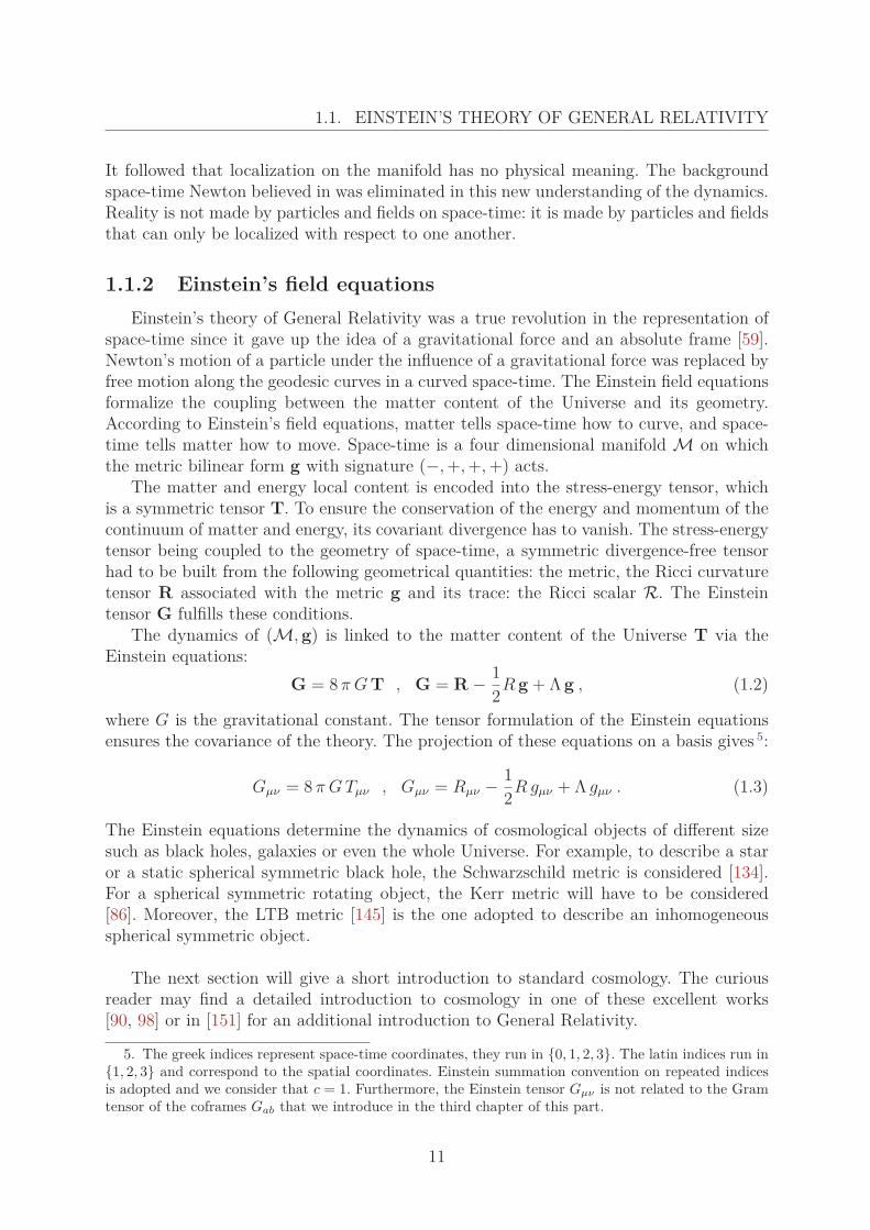
1.1.2 Einstein’s field equationsEinstein’s theory of General Relativity was a true revolution in the representation of
space-time since it gave up the idea of a gravitational force and an absolute frame [59].Newton’s motion of a particle under the influence of a gravitational force was replaced byfree motion along the geodesic curves in a curved space-time. The Einstein field equationsformalize the coupling between the matter content of the Universe and its geometry.According to Einstein’s field equations, matter tells space-time how to curve, and space-time tells matter how to move. Space-time is a four dimensional manifold M on whichthe metric bilinear form g with signature (−, +, +, +) acts.
The matter and energy local content is encoded into the stress-energy tensor, whichis a symmetric tensor T. To ensure the conservation of the energy and momentum of thecontinuum of matter and energy, its covariant divergence has to vanish. The stress-energytensor being coupled to the geometry of space-time, a symmetric divergence-free tensorhad to be built from the following geometrical quantities: the metric, the Ricci curvaturetensor R associated with the metric g and its trace: the Ricci scalar R. The Einsteintensor G fulfills these conditions.
The dynamics of (M, g) is linked to the matter content of the Universe T via theEinstein equations:
G = 8 π G T , G = R − 12R g + Λ g , (1.2)
where G is the gravitational constant. The tensor formulation of the Einstein equationsensures the covariance of the theory. The projection of these equations on a basis gives 5:
Gμν = 8 π G Tμν , Gμν = Rμν − 12R gμν + Λ gμν . (1.3)
The Einstein equations determine the dynamics of cosmological objects of different sizesuch as black holes, galaxies or even the whole Universe. For example, to describe a staror a static spherical symmetric black hole, the Schwarzschild metric is considered [134].For a spherical symmetric rotating object, the Kerr metric will have to be considered[86]. Moreover, the LTB metric [145] is the one adopted to describe an inhomogeneousspherical symmetric object.
The next section will give a short introduction to standard cosmology. The curiousreader may find a detailed introduction to cosmology in one of these excellent works[90, 98] or in [151] for an additional introduction to General Relativity.
5. The greek indices represent space-time coordinates, they run in {0, 1, 2, 3}. The latin indices run in{1, 2, 3} and correspond to the spatial coordinates. Einstein summation convention on repeated indicesis adopted and we consider that c = 1. Furthermore, the Einstein tensor Gμν is not related to the Gramtensor of the coframes Gab that we introduce in the third chapter of this part.
11
CHAPTER 1. GENERAL RELATIVITY AND THE STANDARD MODEL OFCOSMOLOGY
1.2 Homogeneous and Isotropic Cosmology
Once he had built General Relativity, Einstein realized that he could apply it to thefull Universe as a single object. Thereafter, cosmologists quickly developed a cosmologicalmodel based on strong hypothesis: spatial homogeneity and isotropy. This model is theStandard Model of Cosmology (SMC).
In this section, will first present the observational grounds on which the homogeneousisotropic and expanding universe model is based. The spatial length above which theUniverse can be considered as homogeneous and isotropic is indeed still debated. Then,we will explain how Hubble’s observations (or actually Lemaître’s observational analysis)combined with Slipher’s redshift data led to the idea of an expanding universe. Afterwards,we will give the adapted metric to describe a homogeneous isotropic space-time in polarcoordinates, namely the FLRW metric. We will show how the Hubble parameter is linkedto the scale factor and obtain from the Einstein equations and the Bianchi identities theconservation of the energy and momentum and the Friedmann equations. Then, we willintroduce the cosmological parameters, which are the parameters of the SMC .
1.2.1 The Cosmological Principle and the Hubble law
The Cosmological Principle
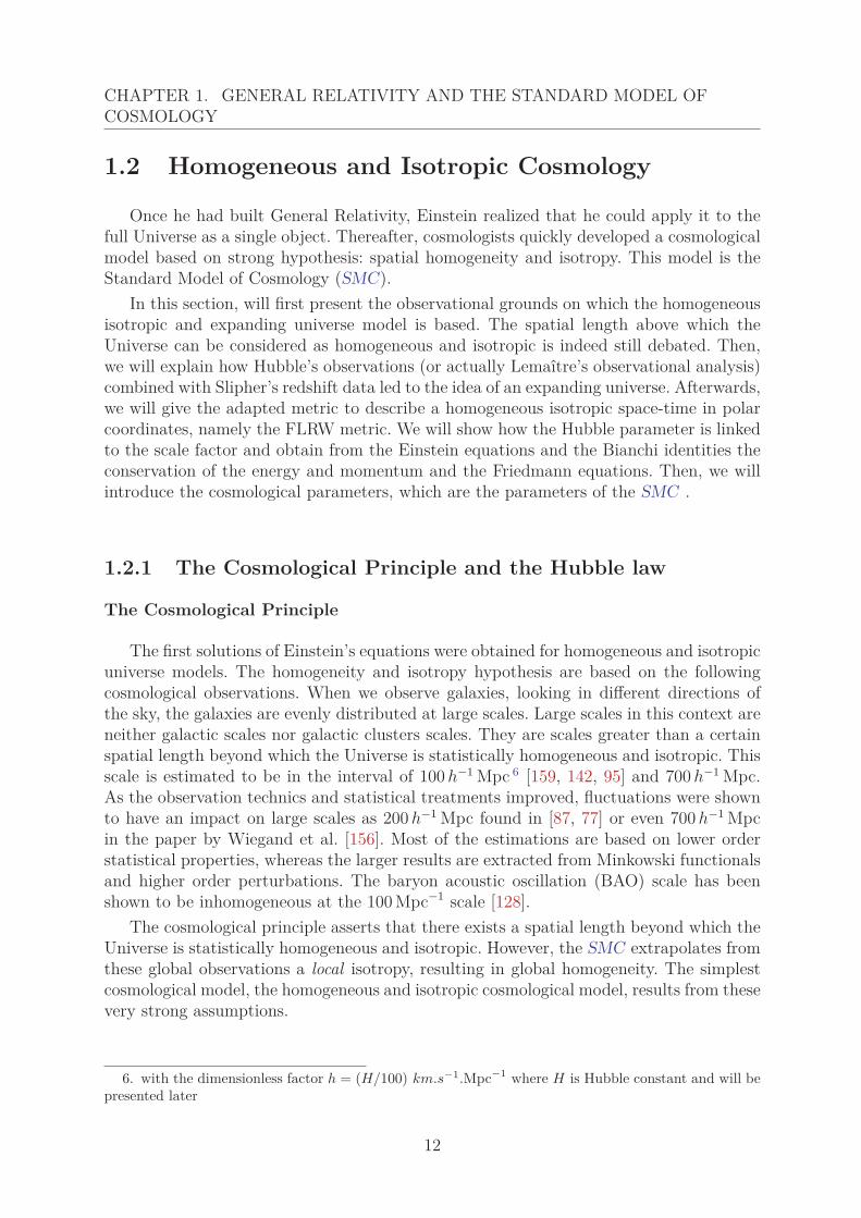
The first solutions of Einstein’s equations were obtained for homogeneous and isotropicuniverse models. The homogeneity and isotropy hypothesis are based on the followingcosmological observations. When we observe galaxies, looking in different directions ofthe sky, the galaxies are evenly distributed at large scales. Large scales in this context areneither galactic scales nor galactic clusters scales. They are scales greater than a certainspatial length beyond which the Universe is statistically homogeneous and isotropic. Thisscale is estimated to be in the interval of 100 h−1 Mpc 6 [159, 142, 95] and 700 h−1 Mpc.As the observation technics and statistical treatments improved, fluctuations were shownto have an impact on large scales as 200 h−1 Mpc found in [87, 77] or even 700 h−1 Mpcin the paper by Wiegand et al. [156]. Most of the estimations are based on lower orderstatistical properties, whereas the larger results are extracted from Minkowski functionalsand higher order perturbations. The baryon acoustic oscillation (BAO) scale has beenshown to be inhomogeneous at the 100 Mpc−1 scale [128].
The cosmological principle asserts that there exists a spatial length beyond which theUniverse is statistically homogeneous and isotropic. However, the SMC extrapolates fromthese global observations a local isotropy, resulting in global homogeneity. The simplestcosmological model, the homogeneous and isotropic cosmological model, results from thesevery strong assumptions.
6. with the dimensionless factor h = (H/100) km.s−1.Mpc−1 where H is Hubble constant and will bepresented later
12
1.2. HOMOGENEOUS AND ISOTROPIC COSMOLOGY
Expanding Universe and the Hubble law
Hubble published in 1929 a study based on 18 galaxies (in which cepheids could beseen) which showed that the speed of galaxies along the line of sight, or equivalently,their redshift, was proportional to their distance. To do so, he combined the relationbetween the luminosity of the cepheids and their distance to the recessional velocities ofthe galaxies in which these cepheids were. This quantity was calculated by Vesto Slipherthrough the use of the redshift. However, Georges Lemaître was actually the first one toobtain these conclusions. His article was published in French two years before Hubble’sand was based on Slipher’s same redshift data and Hubble’s calculated distances. Thecoefficient of proportionality, H, is called the Hubble parameter.
In 1998, two teams, the Supernova Cosmology Project [118], and the High-z SupernovaSearch team [124], reported that, interpreting their data within the SMC , the Universe isnot only expanding, but also accelerating. As we will see in the next part, within the SMC, the acceleration of the expansion of the Universe requires the mass-energy density of theUniverse to be dominated at the present time by a gravitationally repulsive component:the cosmological constant Λ.
1.2.2 Homogeneous and isotropic universe models
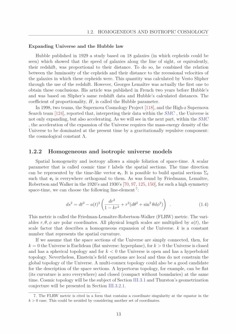
Spatial homogeneity and isotropy allows a simple foliation of space-time. A scalarparameter that is called cosmic time t labels the spatial sections. The time directioncan be represented by the time-like vector et. It is possible to build spatial sections Σt
such that et is everywhere orthogonal to them. As was found by Friedmann, Lemaître,Robertson and Walker in the 1920’s and 1930’s [70, 97, 125, 150], for such a high symmetryspace-time, we can choose the following line-element 7:
ds2 = dt2 − a(t)2(
dr2
1 − kr2 + r2(dθ2 + sin2 θdφ2))
. (1.4)
This metric is called the Friedman-Lemaître-Robertson-Walker (FLRW) metric. The vari-ables r, θ, φ are polar coordinates. All physical length scales are multiplied by a(t), thescale factor that describes a homogeneous expansion of the Universe. k is a constantnumber that represents the spatial curvature.
If we assume that the space sections of the Universe are simply connected, then, fork = 0 the Universe is Euclidean (flat universe: hyperplane), for k > 0 the Universe is closedand has a spherical topology and for k < 0 the Universe is open and has a hyperboloidtopology. Nevertheless, Einstein’s field equations are local and thus do not constrain theglobal topology of the Universe. A multi-connex topology could also be a good candidatefor the description of the space sections. A hypertorus topology, for example, can be flat(its curvature is zero everywhere) and closed (compact without boundaries) at the sametime. Cosmic topology will be the subject of Section III.3.1 and Thurston’s geometrizationconjecture will be presented in Section III.3.2.1.
7. The FLRW metric is cited in a form that contains a coordinate singularity at the equator in thek > 0 case. This could be avoided by considering another set of coordinates.
13
CHAPTER 1. GENERAL RELATIVITY AND THE STANDARD MODEL OFCOSMOLOGY
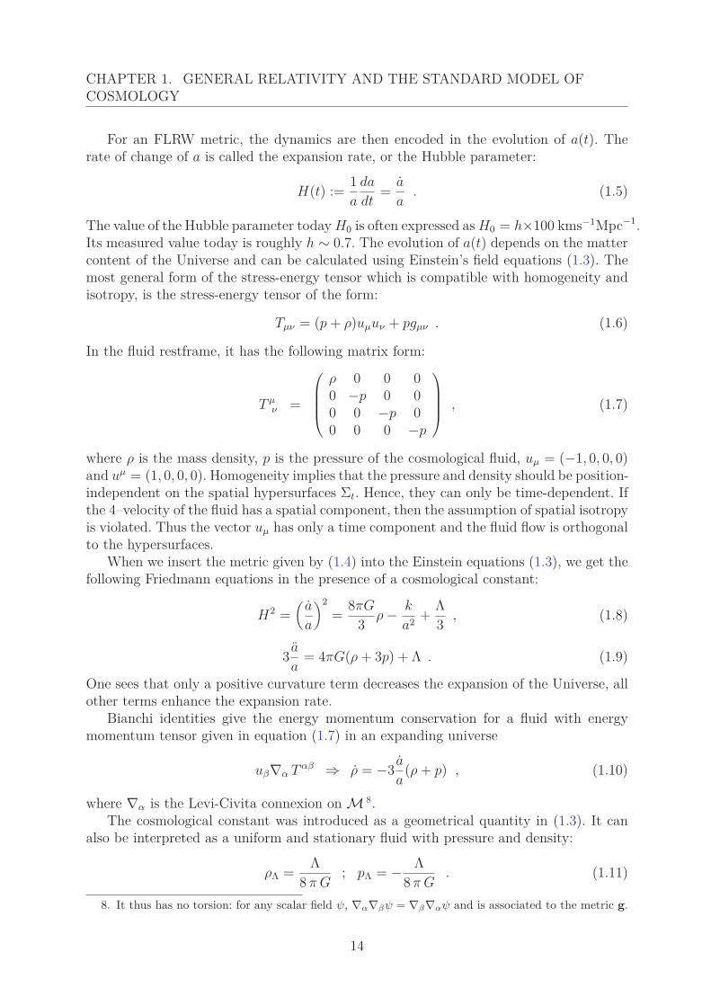
For an FLRW metric, the dynamics are then encoded in the evolution of a(t). Therate of change of a is called the expansion rate, or the Hubble parameter:
H(t) := 1a
da
dt= a
a. (1.5)
The value of the Hubble parameter today H0 is often expressed as H0 = h×100 kms−1Mpc−1.Its measured value today is roughly h ∼ 0.7. The evolution of a(t) depends on the mattercontent of the Universe and can be calculated using Einstein’s field equations (1.3). Themost general form of the stress-energy tensor which is compatible with homogeneity andisotropy, is the stress-energy tensor of the form:
Tμν = (p + ρ)uμuν + pgμν . (1.6)
In the fluid restframe, it has the following matrix form:
T μν =
⎛⎜⎜⎜⎝
ρ 0 0 00 −p 0 00 0 −p 00 0 0 −p
⎞⎟⎟⎟⎠ , (1.7)
where ρ is the mass density, p is the pressure of the cosmological fluid, uμ = (−1, 0, 0, 0)and uμ = (1, 0, 0, 0). Homogeneity implies that the pressure and density should be position-independent on the spatial hypersurfaces Σt. Hence, they can only be time-dependent. Ifthe 4–velocity of the fluid has a spatial component, then the assumption of spatial isotropyis violated. Thus the vector uμ has only a time component and the fluid flow is orthogonalto the hypersurfaces.
When we insert the metric given by (1.4) into the Einstein equations (1.3), we get thefollowing Friedmann equations in the presence of a cosmological constant:
H2 =(
a
a
)2= 8πG
3 ρ − k
a2 + Λ3 , (1.8)
3 a
a= 4πG(ρ + 3p) + Λ . (1.9)
One sees that only a positive curvature term decreases the expansion of the Universe, allother terms enhance the expansion rate.
Bianchi identities give the energy momentum conservation for a fluid with energymomentum tensor given in equation (1.7) in an expanding universe
uβ∇α T αβ ⇒ ρ = −3 a
a(ρ + p) , (1.10)
where ∇α is the Levi-Civita connexion on M 8.The cosmological constant was introduced as a geometrical quantity in (1.3). It can
also be interpreted as a uniform and stationary fluid with pressure and density:
ρΛ = Λ8 π G
; pΛ = − Λ8 π G
. (1.11)
8. It thus has no torsion: for any scalar field ψ, ∇α∇βψ = ∇β∇αψ and is associated to the metric g.
14
1.2. HOMOGENEOUS AND ISOTROPIC COSMOLOGY
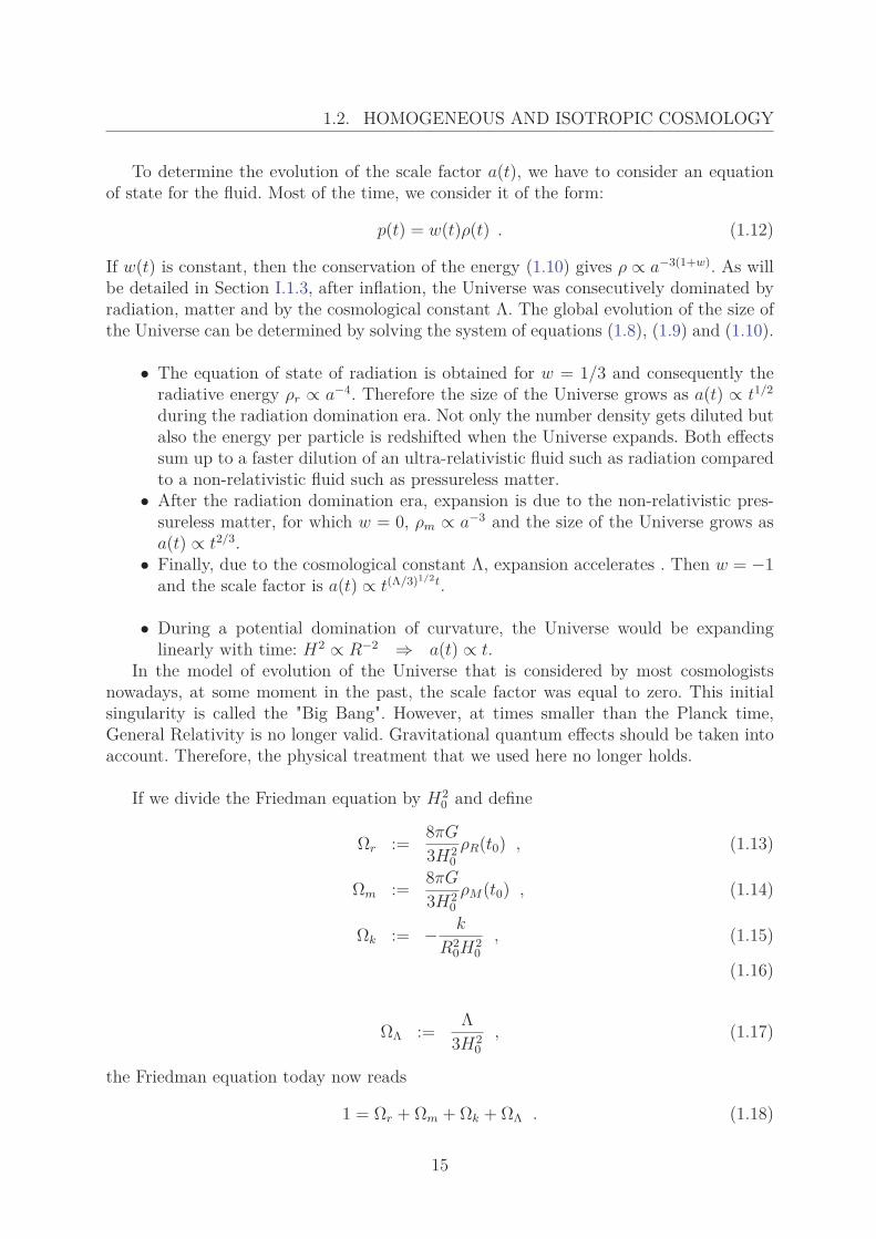
To determine the evolution of the scale factor a(t), we have to consider an equationof state for the fluid. Most of the time, we consider it of the form:
p(t) = w(t)ρ(t) . (1.12)
If w(t) is constant, then the conservation of the energy (1.10) gives ρ ∝ a−3(1+w). As willbe detailed in Section I.1.3, after inflation, the Universe was consecutively dominated byradiation, matter and by the cosmological constant Λ. The global evolution of the size ofthe Universe can be determined by solving the system of equations (1.8), (1.9) and (1.10).
• The equation of state of radiation is obtained for w = 1/3 and consequently theradiative energy ρr ∝ a−4. Therefore the size of the Universe grows as a(t) ∝ t1/2
during the radiation domination era. Not only the number density gets diluted butalso the energy per particle is redshifted when the Universe expands. Both effectssum up to a faster dilution of an ultra-relativistic fluid such as radiation comparedto a non-relativistic fluid such as pressureless matter.
• After the radiation domination era, expansion is due to the non-relativistic pres-sureless matter, for which w = 0, ρm ∝ a−3 and the size of the Universe grows asa(t) ∝ t2/3.
• Finally, due to the cosmological constant Λ, expansion accelerates . Then w = −1and the scale factor is a(t) ∝ t(Λ/3)1/2t.
• During a potential domination of curvature, the Universe would be expandinglinearly with time: H2 ∝ R−2 ⇒ a(t) ∝ t.
In the model of evolution of the Universe that is considered by most cosmologistsnowadays, at some moment in the past, the scale factor was equal to zero. This initialsingularity is called the "Big Bang". However, at times smaller than the Planck time,General Relativity is no longer valid. Gravitational quantum effects should be taken intoaccount. Therefore, the physical treatment that we used here no longer holds.
If we divide the Friedman equation by H20 and define
Ωr := 8πG
3H20
ρR(t0) , (1.13)
Ωm := 8πG
3H20
ρM(t0) , (1.14)
Ωk := − k
R20H2
0, (1.15)
(1.16)
ΩΛ := Λ3H2
0, (1.17)
the Friedman equation today now reads
1 = Ωr + Ωm + Ωk + ΩΛ . (1.18)
15
CHAPTER 1. GENERAL RELATIVITY AND THE STANDARD MODEL OFCOSMOLOGY
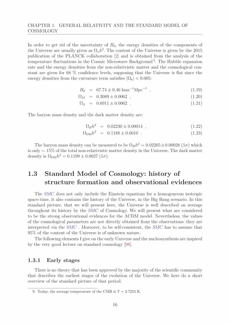
In order to get rid of the uncertainty of H0, the energy densities of the components ofthe Universe are usually given as Ωxh2. The content of the Universe is given by the 2015publication of the PLANCK collaboration [2] and is obtained from the analysis of thetemperature fluctuations in the Cosmic Microwave Background 9. The Hubble expansionrate and the energy densities from the non-relativistic matter and the cosmological con-stant are given for 68 % confidence levels, supposing that the Universe is flat since theenergy densities from the curvature term satisfies |Ωk| < 0.005:
H0 = 67.74 ± 0.46 kms−1Mpc−1 , (1.19)ΩM = 0.3089 ± 0.0062 , (1.20)ΩΛ = 0.6911 ± 0.0062 . (1.21)
The baryon mass density and the dark matter density are:
ΩBh2 = 0.02230 ± 0.00014 , (1.22)ΩDMh2 = 0.1188 ± 0.0010 . (1.23)
The baryon mass density can be measured to be ΩBh2 = 0.02205±0.00028 (1σ) whichis only ∼ 15% of the total non-relativistic matter density in the Universe. The dark matterdensity is ΩDMh2 = 0.1199 ± 0.0027 (1σ).
1.3 Standard Model of Cosmology: history ofstructure formation and observational evidences
The SMC does not only include the Einstein equations for a homogeneous isotropicspace-time, it also contains the history of the Universe, in the Big Bang scenario. In thisstandard picture, that we will present here, the Universe is well described on averagethroughout its history by the SMC of Cosmology. We will present what are consideredto be the strong observational evidences for the ΛCDM model. Nevertheless, the valuesof the cosmological parameters are not directly obtained from the observations: they areinterpreted via the SMC . Moreover, to be self-consistent, the SMC has to assume that95% of the content of the Universe is of unknown nature.
The following elements I give on the early Universe and the nucleosynthesis are inspiredby the very good lecture on standard cosmology [98].
1.3.1 Early stages
There is no theory that has been approved by the majority of the scientific communitythat describes the earliest stages of the evolution of the Universe. We here do a shortoverview of the standard picture of that period.
9. Today, the average temperature of the CMB is T = 2.7255 K.
16
1.3. STANDARD MODEL OF COSMOLOGY AND STRUCTURE FORMATION
The Planck Era
Just after the Big Bang, the fluctuations are so significant that a quantum theory ofgravity is needed to describe the physics of the Universe. This quantum description isnecessary until tP l, the Planck time, which is
tP l =√�G
c3 = 5.4 · 10−44s . (1.24)
At the time before tP l, the Universe was filled with a plasma of relativistic elementaryparticles 10, including quarks, leptons, gauge bosons. We think that the Universe existedin a state of fluctuating chaos during this era. Time was not a well defined quantity, andthe curvature and the topology of space fluctuated very much.
The Inflationary Era
Shortly after the Planck era, the Universe went through a phase of accelerated expan-sion, called inflation, during which the Universe was expanding exponentially:a(t) = exp(Hinfl t). During this era, the energy content of the Universe was dominatedby the potential energy of the inflaton, a scalar field that has negligible kinetic energy.Inflation ended when the inflaton oscillated around its minimum of potential. It thendecayed into the particles of the Standard Model of Particles, which were produced withhigh kinetic energy. After inflation, the Universe was dominated by radiation since theparticles formed a thermal bath of relativistic particles. The inflationary era lasted 10−33s.
At this point, the particles have no mass and quickly interact with other particles.Quarks are free particles and are not confined into hadrons.
At T ∼ 100 GeV, the electroweak symmetry is spontaneously broken and the particlesacquire their mass. Heavy particles become quickly non-relativistic.
At T ∼ 100 MeV the QCD phase transition occurs: quarks are confined into hadrons.
Baryonic asymmetry
If baryon number was conserved during inflation, the number of baryons and an-tibaryons would be the same. They would then annihilate into photons : b + b ↔ nγ .Then, the Universe would be filled with radiation and no matter.
At temperatures bigger then the baryonic mass, photons have enough energy to pro-duce pairs of bb. When the temperature drops below it, photons no longer recreate bb.The number of baryons and antibaryons drops since they annihilate. Baryon number musthave been violated at some point since we observe baryonic matter in the Universe today.Nevertheless, the original asymmetry was very small: nb−n
b
nb+nb
� 10−9 .
At a temperature T ∼ 10 MeV, only the over-density of baryons is left. Non-relativisticprotons and neutrons dominate the matter content and neutrons can decay into protonsby β decay n → p + e− + νe. The reverse process being possible, the ratio of protons and
10. The corresponding temperature is TP l � 1032 K.
17
CHAPTER 1. GENERAL RELATIVITY AND THE STANDARD MODEL OFCOSMOLOGY
neutrons is constant. Furthermore, electrons and anti-electrons are still relativistic whileneutrinos and antineutrinos are thermalized by the weak interaction.
As the temperature drops, the neutrinos decouple. From then on, their density getsonly diluted by the expansion of the Universe. Then, electrons become non-relativistic andannihilate until their number density is equal to the proton number density from chargeconservation. Photons are the only relativistic species in the bath and their temperaturescales until today in the same way as the neutrino temperature.
Nucleosynthesis
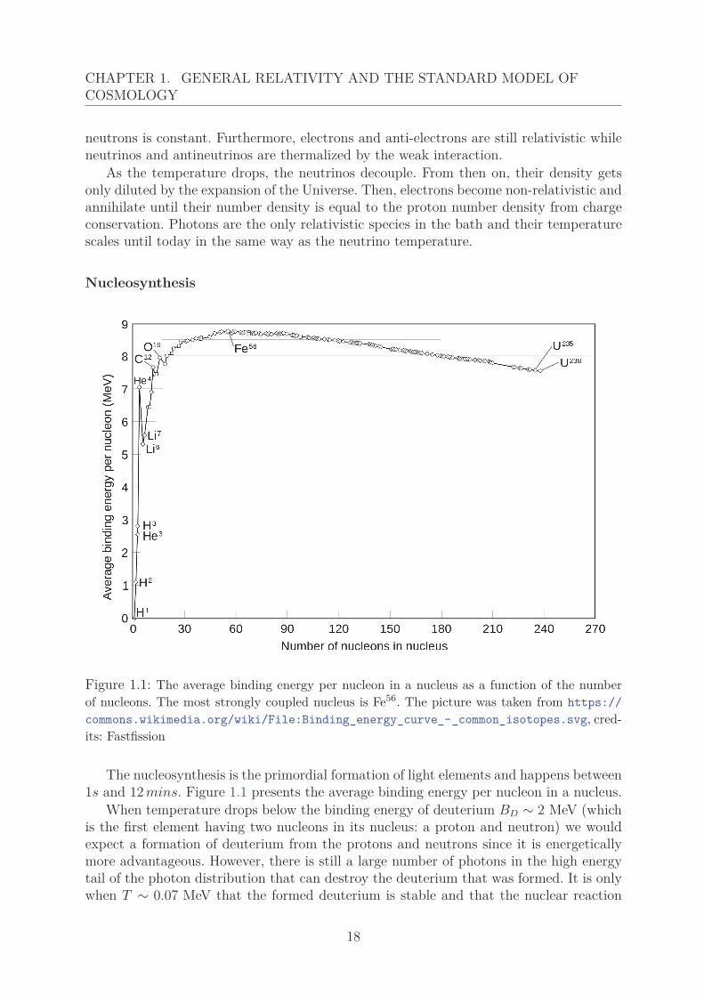
Figure 1.1: The average binding energy per nucleon in a nucleus as a function of the numberof nucleons. The most strongly coupled nucleus is Fe56. The picture was taken from https://commons.wikimedia.org/wiki/File:Binding_energy_curve_-_common_isotopes.svg, cred-its: Fastfission
The nucleosynthesis is the primordial formation of light elements and happens between1s and 12 mins. Figure 1.1 presents the average binding energy per nucleon in a nucleus.
When temperature drops below the binding energy of deuterium BD ∼ 2 MeV (whichis the first element having two nucleons in its nucleus: a proton and neutron) we wouldexpect a formation of deuterium from the protons and neutrons since it is energeticallymore advantageous. However, there is still a large number of photons in the high energytail of the photon distribution that can destroy the deuterium that was formed. It is onlywhen T ∼ 0.07 MeV that the formed deuterium is stable and that the nuclear reaction
18
1.3. STANDARD MODEL OF COSMOLOGY AND STRUCTURE FORMATION
chain can take place:
p + n ↔ D + γ
D + D → 3He + n (1.25)3He + D → 4He + p
· · · (1.26)
Fe56 has the highest binding energy per nucleon but the number densities of intermediatenuclei are not high enough to form Fe56. Nucleosynthesis stops around 4He and only veryfew Li and heavier elements are formed because of the local maximum at 4He 11 .
The next stage in the evolution of the Universe is the matter-radiation equality.For T ∼ 1 eV, the matter and radiation have comparable energy densities. When
temperature lowers, matter begins to dominate.After nucleosynthesis, photons, electrons, protons and 4He are still in thermal equilib-
rium since they electromagnetically interact. Around T ∼ 0.25 eV, there are not enoughenergetic photons to enable the ionization of hydrogen. Protons and electrons leave thethermal bath and combine into stable atoms. Thereafter, the Universe no longer containscharged particles. This stage is called recombination. At recombination, photons decouplesince there are no more charged particles to interact with. The photon distribution isfrom that time on only changed by the expansion of the Universe. The remaining photonsform a background radiation, still observable today with a temperature T ≈ 2.7 K. Thisradiation is the Cosmic Microwave Background, that we discuss in the next part.
1.3.2 Decoupling and the CMB anisotropiesFor a good historical introduction on the CMB, the reader may refer to [75]. The
discovery of the Cosmic Microwave Background (CMB) is usually attributed to ArnoPenzias and Robert Wilson in 1965 [116]. As they were trying to build an antenna forradio waves, they measured a uniform excess temperature. Simultaneously, Robert Dicke’sgroup at Princeton had already realized that a hot Big Bang scenario could leave ablackbody radiation filling the Universe [49] of a few Kelvin today. Nevertheless, the CMBcould be dated back to 1941, when McKellar interpreted some interstellar spectroscopicabsorption lines to be due to some excitation radiation from a black body. The blackbody temperature required in order to explain the relative intensities of the observedlines was 2, 3 K. Nevertheless, this result has never been properly discussed because ofworld war two. This discovery represents the most powerful observational constraint onthe parameters of the SMC we have today.
As we have discussed in the previous section, before recombination, hydrogen andother elements were mostly ionized. At recombination, the Universe transitioned fromthis opaque state, to being mainly neutral, and therefore transparent. The photons thendecoupled from matter, when Universe was about 380000 years old. If we assume thatdecoupling was a fast process, then the small fluctuations in the photon temperature
11. To cross the gap a three body reaction is needed 3 × 4He → 12C.
19
CHAPTER 1. GENERAL RELATIVITY AND THE STANDARD MODEL OFCOSMOLOGY
before decoupling are frozen in. Photons propagate freely until today and their spectrumstill contains the fluctuations of the primordial inhomogeneities in the matter repartitionat the moment of decoupling.
The power spectrum of the initial perturbations characterizes the temperature fluc-tuations with respect to the angular scale of the anisotropies. With Planck data [1], thecosmological parameters of the ΛCDM model are being measured with percent level uncer-tainties. They are tuned in order to fit optimally the initial fluctuations obtained from theCMB statistical observations (cf Figure 37 in [1], showing the power spectrum obtainedby the PLANCK collaboration) but also the brightness-redshift relation for supernovae,and the large-scale galaxy clustering. The CMB power spectrum can be obtained theo-retically for scalar adiabatic perturbations taking into account the Sacks-Wolfe effect 12,the BAOs 13 and Silk damping 14.
In this chapter, I presented the historical context in which General Relativity emerged.I discussed the theoretical steps that led to this revolutionary theory, that abandonsNewton’s idea of absolute space and time and asserts that it is gravity that specifiesat each point the inertial motion, thus determining the local inertial frames. Then, Iexplained how the equations for a homogeneous isotropic universe model can be obtainedfrom Einstein’s equations. These equations lie at the basis of the SMC , i.e. ΛCDMmodel. In the third part of this chapter, I presented the history of the Universe untilrecombination in the frame of the Big Bang scenario. This ended in a discussion of theCosmic Microwave Background, which provides us with the observational constraint onthe parameters of the SMC . In the next chapter, we will consider the next stage of theevolution of the Universe: the formation of large scale structures.
12. The photon spectrum is not only redshifted because of expansion. It also contains a shift due tothe gravitational Doppler effect. The difference between the local value of the gravitational potential atemission and detection shifts the wavelength of photons. The gravitational Doppler effect is called theSachs-Wolfe effect.
13. The modes that entered the horizon during radiation domination underwent acoustic oscillationsbecause of the interplay of gravity and pressure. When the photon fluid decouples from baryons theoscillations remain frozen in the spectrum.
14. When we observe a photon from a given direction, it does not exactly carry the information fromthe same direction but from a point a little bit around it. When photons leave equilibrium, they canindeed still scatter elastically and change the direction of their trajectory. This implies that correlationson smaller scales are erased. The power spectrum drops asymptotically to zero for large wave number.
20
Chapter 2
Large Scale Structure Formation
Contents2.1 Vlasov equation and Newtonian Eulerian dynamics . . . . . . 22
2.1.1 The Vlasov-Newton system . . . . . . . . . . . . . . . . . . . . 22Trajectories in phase space and mass conservation . . . . . . . 22Vlasov-Newton equations . . . . . . . . . . . . . . . . . . . . . 23
2.1.2 Structure formation, shell-crossing and velocity dispersion . . . 252.1.3 Eulerian perturbation scheme . . . . . . . . . . . . . . . . . . . 262.1.4 Numerical simulations . . . . . . . . . . . . . . . . . . . . . . . 27
2.2 Newtonian Lagrangian perturbation approach to describestructure formation . . . . . . . . . . . . . . . . . . . . . . . . . 28
2.2.1 Lagrangian description of structure formation . . . . . . . . . . 292.2.2 Lagrange-Newton System . . . . . . . . . . . . . . . . . . . . . 302.2.3 Zel’dovich approximation . . . . . . . . . . . . . . . . . . . . . 302.2.4 Newtonian Lagrangian perturbation theory . . . . . . . . . . . 30
2.3 Relativistic Lagrangian description of structure formation . . 312.3.1 Cartan formalism and the dynamics of space-time . . . . . . . 32
Manifolds and charts . . . . . . . . . . . . . . . . . . . . . . . . 32From coordinates to frames . . . . . . . . . . . . . . . . . . . . 32Differential forms and Cartan coframes . . . . . . . . . . . . . 33
2.3.2 3 + 1 foliation of space-time in a Lagrangian approach . . . . . 34
21
In the last chapter, we explained how the Friedmann equations of the SMC wereobtained from the Einstein equations, assuming a homogeneous isotropic universe. Noexact solution of the Einstein equations can be obtained in general, except for highlysymmetric density profiles. This is the case for the Schwarzchild metric of black holes forexample.
In order to deal with more general cases, we have to build a perturbation theory forthe gravitation equations.
In this chapter, we will first consider Newtonian structure formation in the phasespace. In Section 2.8, we will present the Vlasov-Newton system and then consider thecase of a dust fluid model to obtain the Euler-Newton system. An Eulerian first-orderperturbation solution will be then given in Section I.2.1.3. We will then discuss hownumerical simulations, that mostly use Newtonian perturbation theory, give an interestinginsight into the large scale structure formation (see Section I.2.1.4).
The next section will first present the Lagrangian description of structure formation(Section I.2.2.1) and then discuss how, in many respects, this approach is far more powerfulthen the Eulerian one (Section I.2.2.4).
This will be the major motivation for developing a relativistic Lagrangian perturbationtheory. Therefore, we will discuss the generalization of the Newtonian Lagrangian per-turbation approach to General Relativity in Section I.2.3. We will build the relativisticanalogue of the deformation field and give the major tools that will enable us to developthis approach in the next part.
Since Newtonian gravity and General Relativity share several features, their perturba-tion schemes will exhibit strong similarities. These analogies will be the subject of ChapterII.2.
2.1 Vlasov equation and Newtonian Euleriandynamics
2.1.1 The Vlasov-Newton system
Trajectories in phase space and mass conservation
In this section, we consider Newton’s theory of gravity. We will follow the ideas pre-sented in Thomas Buchert’s M2 lecture course at ENS de Lyon [38] and in [13] to establishthe fundamental equations for cosmological fluids. These equations are used in numeri-cal simulations, as we will discuss in Section I.2.1.4. As we will see, phase space is moreadapted then the Euclidean space R3 to describe fluids with pressure or velocity dispersion.
Fluid particles can either be described in an Eulerian way, where the reference frameis fixed with respect to the fluid flow, or in a Langrangian way, following the fluid flow.Contrary to the Eulerian coordinates (w = (x, v), Eulerian position and velocity), theLagrangian coordinates label the fluid (W = (X, V), Lagrangian position and velocity).If N is the total number of particles in the volume Ωt, d6w the infinitesimal Eulerianvolume, (x, t) the density, m the mass of the particles, then the particle distribution
22
2.1. VLASOV EQUATION AND NEWTONIAN EULERIAN DYNAMICS
function e (w, t) satisfies:
N =∫
Ωt
e (w, t) d6w and (x, t) = m∫
Ωvt
e (w, t) d3v . (2.1)
Ωvt being the restriction of Ωt to the velocity space, the average velocity is defined by :
v(x, t) =∫
Ωvt
e (w, t) v d3v∫Ωv
te (w, t) d3v
. (2.2)
A diffeomorphism k mapping Lagrangian coordinates to the Eulerian ones in the phasespace exists:
k : R6 −→ R6
W −→ w = k(W, t) thus W = k(w, ti) .(2.3)
ti is the initial time. The determinant of the Jacobian matrix for the Eulerian-to-Lagrangiancoordinate transformation is
JΓ = det
(∂ki
∂Wk
)with d6w = JΓ(W, t) d6W . (2.4)
If we generalize the Lagrangian derivative to
D
Dt:= ∂
∂t
∣∣∣∣W
= ∂
∂t
∣∣∣∣w
+ s · ∇w , (2.5)
where s is the generalization of the velocity vector in the phase space:
s(W, t) := D
Dtk(W, t) = ∂
∂t
∣∣∣∣W
k(W, t) , (2.6)
we can show that the conservation of the number of particles DDt
N = 0 implies 1:
D
Dte + e ∇w · s = 0 . (2.7)
Vlasov-Newton equations
The gravitational field g(x, t) does not depend of the velocity field thus 2 ∇w · s =∂vi
∂xi+ ∂gk
∂vk= 0 and the conservation of the number of particles (2.7) becomes:
D
Dte = ∂
∂te + vi
∂
∂xi
e + gi∂
∂vi
e = 0 , (2.8)
1. This comes from the relation on the Jacobian:
D
DtJΓ = JΓ ∇w · s .
2. x and v are independent coordinates.
23
CHAPTER 2. LARGE SCALE STRUCTURE FORMATION
If we add to these equations the field equations of the gravitational field:
∇ × g = 0 ; ∇ · g = Λ − 4 π G m∫
Ωvt
e (w, t) d3v , (2.9)
we obtain the Vlasov-Newton system. A dust fluid matter model has neither velocitydispersion nor pressure. Its particle distribution function is:
e dust(x, v, t) = n(x, t) δ(v − v(x, t)) . (2.10)
We recover the usual continuity equation, which, with the gravitational field equationsgives the Euler-Newton system.
We now consider a homogeneous isotropic Universe filled with dust fluid. We can thusgo back to the Euclidean space R3. We represent by f the diffeomorphism mapping theLagrangian spatial coordinates X which label fluid elements, to the Eulerian ones x, whichare the positions of these elements in Eulerian space at the time t:
f : R3 −→ R3
X −→ x = f(X, t) and X = f(x, ti) .(2.11)
The description in terms of the trajectory function f is only possible before shell-crossing.Once caustics have formed, f is no longer a diffeomorphism and this description breaksdown.
A deeper physical interpretation of the specificity of Lagrangian coordinates will begiven in the next section I.2.2.1.
Homogeneity and isotropy imply f = a(t)X where a(t) is a time dependent functioncalled scale factor. Newton’s second law implies g = a(t)X where we denoted by anoverdot ˙ the time derivative d/dt. Combining the mass conservation equation with thefield equation (2.9), we get Friedmann’s acceleration law:
a(t)a(t) = Λ − 4 πGH . (2.12)
H is the homogeneous density. Integrating this equation gives the Friedmann expansionlaw, which is the fundamental equation of the ΛCDM model:
H2 − 8 π G
3 H − Λ3 + k
a2 = 0 . (2.13)
H(t) = a/a is Hubble expansion factor. We remark that we didn’t use Einstein’s theoryof gravitation to derive this equation.
Let us now look at the moments of Vlasov equation. To do so, we define the followingquantities:
(x, t)vi = m∫
Ωvt
vi e (w, t) d3v : (x, t)vi vj = m∫
Ωvt
vi vj e (w, t) d3v . (2.14)
The 0th moment gives:∂
∂t + ∂
∂xj
(vj) = 0 . (2.15)
24
2.1. VLASOV EQUATION AND NEWTONIAN EULERIAN DYNAMICS
We define the velocity dispersion tensor πij = (vi − vi)(vj − vj) and Πij = (vi − vi)(vj − vj).Then the 1st moment gives the Euler-Jeans equation:
d
dtvi = gi − ∂
∂xj
Πij . (2.16)
The velocity dispersion, defined at each point x can be represented in terms of the eigen-vectors and eigenvalues of the velocity dispersion tensor. If ψi = 1
�Πik,k, the Euler-Jeans
equation can be rewritten:∂
∂tvi + vk vi,k = gi − ψi . (2.17)
If we take the divergence of this equation, we get
d
dtθ = Λ − 4 π G − 1
3θ2 + 2 (ω2 − σ2) − ψi,i , (2.18)
where θ the expansion rate, ω the vorticity and σ the shear are defined locally. To obtainthis equation, we didn’t assume homogeneity, isotropy or any symmetry.
2.1.2 Structure formation, shell-crossing and velocity dispersionThe primordial fluctuations of the CMB I.1.3.2, amplified by gravity, have collapsed
into the large scale structures of the present Universe. Over-dense regions have indeedattracted some matter and emptied under-dense regions. Voids got larger and larger andconfined the matter into sheets. Sheets collapsed into filaments and filaments into clusterswhich virialized to give halos. We want to present the dynamics of a gravitational collapseand explain how, from a fluid without initial velocity dispersion, the several shell-crossingsit will undergo will generate velocity dispersion.
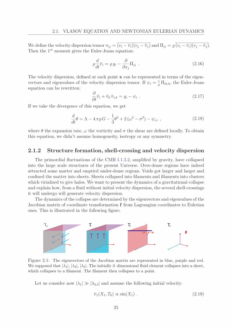
The dynamics of the collapse are determined by the eigenvectors and eigenvalues of theJacobian matrix of coordinate transformation f from Lagrangian coordinates to Eulerianones. This is illustrated in the following figure.
Figure 2.1: The eigenvectors of the Jacobian matrix are represented in blue, purple and red.We supposed that |λ1|, |λ2|, |λ3|. The initially 3–dimensional fluid element collapses into a sheet,which collapses to a filament. The filament then collapses to a point.
Let us consider now |λ1| � |λ2,3| and assume the following initial velocity:
v1(X1, T0) ∝ sin(X1) . (2.19)
25
CHAPTER 2. LARGE SCALE STRUCTURE FORMATION
The gravitational field generated by three streams is bigger then the one generated byone stream. Thus, the wave fronts will cross again, to generate five then seven streams andso on. As the number of streams increases, the ellipsoid of velocities, which was initiallyhighly anisotropic, becomes more and more isotropic.
2.1.3 Eulerian perturbation schemeWe now consider a fluid without pressure and velocity dispersion. The 0th and 1st
moments of the Vlasov equation associated to the field equations for the gravitationalfield give the Euler-Newton system:
∂v∂t
+ v · ∇v = g , (2.20)∂ρ
∂t+ ∇ · (ρv) = 0 , (2.21)
∇ × g = 0 , (2.22)∇ · g = Λ − 4πGρ . (2.23)
From these equations, it is possible to obtain an evolution equation for the vorticityω = 1
2∇ × v. This equation is called Helmholtz transport equation for the vorticity:
d
dt
(ω
ρ
)=[
ω
ρ· ∇
]v . (2.24)
Combining this equation with the continuity equation, we can show that the solution is
ω = Ω · ∇0fJ
; Ω := ω(X, ti) , (2.25)
where J is the determinant of the Eulerian-to-Lagrangian Jacobian matrix.
We introduce the comoving coordinates q = x/a(t). They coincide with the Lagrangiancoordinates when the fluid undergoes a homogeneous and isotropic expansion. In whatfollows, we consider inhomogeneous deformations of the form:
q = X + P(X, t) , (2.26)
where the magnitude of P(X, t) must not be small. In the Eulerian perturbation approach,we split the following fields into background fields, associated with the Hubble flow andsolution of Friedmann’s equations, and peculiar fields.
ρ(q, t) =: ρH(t)(1 + δ(q, t)) , (2.27)v(q, t) =: vH + u(q, t) ; vH(t) := a q , (2.28)g(q, t) =: gH + w(q, t) ; gH(t) := a q . (2.29)
δ(q, t), u and w are respectively the density contrast, the peculiar velocity and the peculiaracceleration. The Euler-Newton system can be split into the background dynamics and
26
2.1. VLASOV EQUATION AND NEWTONIAN EULERIAN DYNAMICS
equations for peculiar fields. If we now assume that the deviation fields are first-orderperturbations 3, the first-order equations for the peculiar fields are
∂
∂t
∣∣∣qδ + 1
a∇q · u = 0 , (2.30)
∂
∂t
∣∣∣qu + Hu = w , (2.31)
∇q × w = 0 , (2.32)∇q · w = −4πGaρH δ . (2.33)
The Eulerian perturbation theory was first formalized by Peebles in [115]. The solutionsto these equations for an Einstein-de-Sitter Universe (k = 0, Λ = 0) are:
w = 23ti
2
(t
ti
)−2/3A(q) + 2
3ti2
(t
ti
)−7/3B(q) , (2.34)
u = 23ti
(t
ti
)1/3A(q) − 1
ti
(t
ti
)−4/3B(q) , (2.35)
δ = −(
t
ti
)2/3∇q · A(q) −
(t
ti
)−1∇q · B(q) , (2.36)
where
A(q) = 35Uti + 9
10Wti2 , (2.37)
B(q) = −35Uti + 3
5Wti2 , (2.38)
andU := u(q, ti) ; W := w(q, ti) . (2.39)
Initial data is often given in terms of the Fourier transform of the initial density contrast.
2.1.4 Numerical simulationsA powerful insight into the physics of large scale structures is provided by numerical
simulations. Cosmological simulations are based on the ΛCDM model and Newtoniangravity. They take into account the homogeneous expansion of the Universe and assumea given set of cosmological parameters.
Cosmological dark matter simulations don’t consider baryonic matter since, accord-ing to the ΛCDM model, it is small with respect to the amount of dark matter. Theyuse a dust fluid model for dark matter and are able to predict the evolution of largescale structures accurately up to the non-linear regime. They simulate systems from thecosmic scales (� 20 Gpc) to the cluster and galactic scales (� 10 pc) and involve un-til 5.1011 particles of dark matter, as is done in DEUS Full Universe Run simulationbased on RAMSES code [17]. Simulations of the DEUS Full Universe Run for different
3. We see that, in the Eulerian perturbation theory, from the definition of the peculiar fields (2.29),we cannot describe high density contrast because the density field is a perturbed variable.
27
CHAPTER 2. LARGE SCALE STRUCTURE FORMATION
box sizes and redshifts can be found at http://www.deus-consortium.org/a-propos/dark-energy-universe-simulation-full-universe-run/.
Even if dark matter-only simulations are often used as a basis for semi-analytical mod-els, their relevance ends when we go to galactic scales, where the baryonic effects are tooimportant to be neglected. The baryonic effects could indeed have a strong impact on thedistribution of dark matter in galactic halos. Furthermore, deviations from the mean-fieldapproximation that is used by the solution of Poisson’s equations, then become significant[32]. [94] is an excellent review on the state of the art in cosmological simulations.
Hydrodynamical simulations describe the baryonic component of the Universe. Thesesimulations either solve Euler equations for a gas on a grid (which can be adaptative- Adaptative Mesh Refinement - as is done in RAMSES [140]) or can describe the gasas a set of particles, as is done in "Smooth Particle Hydrodynamics" SPH codes such asGADGET [137].
Once the initial conditions, coming from the CMB, are implemented, different methodscan be used to solve Euler equations. The direct summation method, known as Particle-Particle method, evaluates the force on each particle by summing the interaction exertedby the neighbors. The tree-code method, used in RAMSES code, consists in decomposinghierarchically the influence of the neighboring structures and treating the influence ofremote structures by a multipole expansion on clusters containing many particles. Theexpansion can thus be truncated at low order. Other methods exist, as is explained in[13].
The description of the evolution of structures is enriched by taking into account theradiative and thermal transfers (as is done in RAMSES [140] by Godunov method, a mod-ern shock-capturing scheme that describes the thermal history of the fluid), the chemicalreactions or the impact of magnetic fields on plasmas. Then, these simulations allow agood precision estimation of the baryonic mass-to-light function of galaxies. The submeshphysics, which includes, for example, the stellar formation, supernovae explosions or theactive galactic nucleus are usually described as an overall feedback.
Some cosmologists claim that analytical approaches have arrived at their limits whilewe will show that numerical and analytical approaches are complementary in the de-scription of structure formation. The intrinsic Lagrangian analytical approach will givea powerful insight into the large-scale structure formation and shed a new light on thedynamics of the Universe.
2.2 Newtonian Lagrangian perturbation approach todescribe structure formation
We here present a Lagrangian theory for self gravitational flows following [38] and[26]. Contrary to the Eulerian case, a single variable is needed to describe the gravitationdynamics: the trajectory function f , presented in (2.11). Density and velocity are no longerdynamical variables and thus high density contrasts can be described by this method. Wewill derive the Lagrange-Newton system, which is a closed set of Lagrangian equationsfor the trajectory field f describing the gravitational dynamics of the self-gravitatingflow. As we will show, we can go back to the Euler-Newton system from the Lagrange-
28
2.2. NEWTONIAN LAGRANGIAN PERTURBATION APPROACH TO DESCRIBESTRUCTURE FORMATION
Newton system as long as the mapping f is invertible and non-singular. This conditionwill be expressed in terms of J , the determinant of the Jacobian matrix of the Eulerian-to-Lagrangian coordinate transformation.
2.2.1 Lagrangian description of structure formationThe trajectory field of fluid elements, also called deformation field, has been defined in
(2.11). In the Lagrangian approach, the Eulerian position f(X, t) and time t are no longerindependent variables. The independent variables are now (X, t). The tensor of the firstderivatives of the trajectory field with respect to the Lagrangian coordinates: (fi|j), calledthe Jacobian matrix, measures the deformation of the fluid particle. Its determinant isgiven by:
J := det(
∂fi
∂Xj
(X, t))
= 16εijkεklmf i
|kf j|lf
k|m . (2.40)
We have denoted by a vertical slash |j the spatial derivative with respect to Xi, by anoverdot ˙ the time derivative and have used Einstein summation convention on repeatedindices: ui vi = u1 v1 + u2 v2 + u3 v3 and uμ vμ = u0 v0 + u1 v1 + u2 v2 + u3 v3 . εijk isthe Levi-Civita tensor. It is equal to 1 if {i, j, k} are an even permutation of {1, 2, 3},−1 if they are an odd permutation of {1, 2, 3} and zero otherwise. We link the Eulerianposition, velocity and acceleration to the trajectory function by:
x := f(X, t) ; v := f(X, t) ; g := f(X, t) . (2.41)
In the Lagrangian perspective, the volume of the deformed fluid element is measured bythe determinant of the Jacobian matrix J(X, t) = det(fi|j). The density must thereforebe proportional to its inverse.
ρ(X, t) = ρ(X, ti)J(X, t) . (2.42)
This comes from the fact that the Jacobian is solution of the following equation:
J = J ∇v . (2.43)
It is initially equal to J(X, ti) = 1 since by definition, Eulerian coordinates initiallycoincide with Lagrangian ones.
The inverse map to f is defined by h = f−1. It is possible to check that its gradient isgiven by 4
X = h(x, t) , hi,j = 1
2Jεjpqε
ilmfp|lf
q|m . (2.44)
We denoted by ,i the Eulerian derivative with respect to xi.
4. This can be easily proved in the 2–dimensionnal case, where the inverse Jacobian matrix is
J−1ab (2D) =
1J(2D)
(f2|2 −f1|2
−f2|1 f1|1
)
where the Jacobian is J(2D) = f2|2f1|1 − f2|1f1|2 .
29
CHAPTER 2. LARGE SCALE STRUCTURE FORMATION
2.2.2 Lagrange-Newton SystemIn order to formulate Euler-Newton system in terms of the Lagrangian trajectory
function, we introduce the following notation. We denote by J (A, B, C) the functionaldeterminant of A(X, t), B(X, t) and C(X, t)
J (A, B, C) = εklmA|kB|lC|m . (2.45)
From the composition of the derivatives and from (2.44), for any field ai we have
ai,j = ai|khk,j = 1
2JεjpqJ (ai, fp, f q) . (2.46)
We denote by g[i,j] the antisymmetric part of gi,j : g[i,j] = 12 (gi,j − gj,i). If we replace
the gravitational field by the second time derivative of the trajectory function f(X, t) (cf(2.41)) in the field equations, we get from (2.46) the following equations:
g[i,j] = (∇ × g)k = 12J
εpq[jJ (fi], fp, f q) = 0 ,
gi,i = 1
2JεipqJ (f i, fp, f q) = Λ − 4πGρ .
(2.47)
The first one can be rewritten as
εpq[jJ (fi], fp, f q) = 0 which is equivalent to δij fi|[pf j
|q] = 0 . (2.48)
Later, we will show that these equations have relativistic counterparts. The relativisticequations will no longer be expressed in terms of the 3 components of the trajectoryfunction f , but in terms of the nine components of the Cartan coframes.
2.2.3 Zel’dovich approximationThe Zel’dovich approximation [161] has been built from the observation that, for a
sufficiently long time, a gravitational collapse exhibits a preferred direction. This directioncorresponds to the eigenvector of the Jacobian matrix associated to the largest eigenvalue(|λ1| in Fig. 2.1). This collapse leads to the formation of flat structures (pancakes), thento filaments and finally to clusters. For each stage of the collapse, we can assume thatthe velocity and the acceleration fields are approximately collinear. A subclass of solu-tions can then be investigated [21]. The success of the Zel’dovich approximation in theNewtonian Lagrangian setup is a strong motivation to develop it in the relativistic frame.Nevertheless, since no relativistic numerical simulations exist, a relativistic Zel’dovichapproximation has not yet been implemented.
2.2.4 Newtonian Lagrangian perturbation theoryMajor differences exist between the Eulerian perturbation approach and the Lagrangian
one. They are the motivations for developing the Lagrangian approach. First, the densityfield is not a perturbation variable, contrary to the Eulerian case. Second, the perturbed
30
2.3. RELATIVISTIC LAGRANGIAN DESCRIPTION OF STRUCTUREFORMATION
flow f is a function of the Lagrangian coordinates, which follow the flow whereas in theEulerian case, the perturbations are expressed in the frame associated to the homogeneousflow. Deviations to the homogeneous flow may be small but the Eulerian fields evaluatedalong the perturbed flow can experience large changes as is represented and discussed inFigure 2 of [26].
The perturbed trajectory field is the sum of a homogeneous background trajectoryfield and of an inhomogeneous perturbation field:
f(X, t) = a(t) (X + P(X, t)) . (2.49)
The inhomogeneous perturbations can be decomposed into different orders, order n beingnegligible with respect to order n−1. A discussion of the perturbation and solution schemewill be provided in Chapter II.2.
A reason for the strong success of analytical Lagrangian description of structure for-mation is that it intrinsically contains non-linear Eulerian terms. The efficiency of thisapproach has been discussed in [153], where the authors compare the density profile ob-tained from a particle-mesh Newtonian simulation, based on the iterative resolution ofPoisson equations, to the density profile obtained from the second order solutions of theLagrange-Newton system. Both are computed for a box of a size of (200h−1 Mpc)3 andfrom the CMB initial data. The first method requires a numerical resolution whereas thesecond is just the plotting of analytical functions. Both are in very good agreement asdiscussed in [109].
Nevertheless, the Lagrangian scheme has an intrinsic limit: it is no longer accurateonce the shell-crossing has taken place. In order to follow the perturbation scheme afterthat time, we have to truncate the high-frequency modes in the initial fluctuation spec-trum. Thus, under a certain characteristic size (� galaxy group mass scale), the approachbreaks down [108]. For further details on the Newtonian perturbation theory, the readercan refer to [27, 55].
2.3 Relativistic Lagrangian description of structureformation
In last section, we have presented the Newtonian Lagrangian perturbation theory. Wehave seen that the Lagrangian description is much more powerful then the Eulerian one,even when Lagrangian analytical perturbation solutions are compared to Eulerian numer-ical simulations. These outcomes strongly support the search for a relativistic generaliza-tion of the Lagrangian approach. Such a generalization was first suggested by Kasai [85]and was further investigated for the non-perturbative regime in [35] by Thomas Buchertand Matthias Ostermann, where they build a Lagrangian framework for the descriptionof structure formation in General Relativity and define the relativistic generalization ofthe Zel’dovich approximation. Nevertheless, some work has still to be done for the devel-opment of the intrinsic Lagrangian perturbation formalism. In this chapter, I will give thebasic mathematical notions of differential geometry needed to describe structure formationon a curved manifold.
31
CHAPTER 2. LARGE SCALE STRUCTURE FORMATION
I will try to give a physical intuition for the Cartan frames and explain how Cartancoframes can be obtained from them. Then, we will discuss why these coframes are therelativistic counterparts of the gradient of the trajectory function. The Cartan formal-ism will be the accurate one to describe the relativistic dynamics of space-time in theLagrangian way.
2.3.1 Cartan formalism and the dynamics of space-timeWe present the tools needed to understand the Cartan coframe formulation of General
Relativity in the Lagrangian description. The reader seeking for a more detailed andcomplete introduction to the mathematical tools needed for General Relativity can findfurther information in these very good books [75] [74] [130].
Manifolds and charts
Space-time is a four dimensional manifold M to which is associated the metric bilinearform g with signature (−, +, +, +). A 4-dimensional manifold M is a topological spacethat is locally homeomorphic to Euclidean space 5 6
R4. This means that there exists a
family of open neighborhoods Ui together with continuous one-to-one mappingsfi : Ui → R4 with a continuous inverse such that this family of open neighborhoods coversthe whole manifold : ⋃
i
Ui = M . (2.50)
If P is a point in M and U an open neighborhood of P , there exists a mapping φ : U → R4
such that φ(P ) = (x0, x1, x2, x3) will be a vector in R4. This mapping φ is a coordinatesystem, also called coordinate chart.
Usually, it is not possible to cover a manifold with a single chart such that everypoint of space-time has a unique coordinate. For S2, the 2-sphere, 2-dimensional surfaceof the 3-dimensional sphere, the lines of constant coordinate must cross somewhere on S2.Therefore, at least two charts are required to cover it. At the overlapping of two charts,General Relativity requires that the mapping between the coordinates of the overlappingcharts is at least doubly differentiable.
From coordinates to frames
Gravity can be seen as the field that determines at each point of space-time thepreferred frame in which the motion is inertial. Consider now a particular event associatedto the point A on the space-time manifold. Let xA be its coordinates. Consider the localinertial frame around A and denote by Aχ the coordinates it defines in some arbitrarycoordinate map x = {xμ}. Choose the origin such that Aχ(A) = 0. As explained in theSection I.1.1.1, the motion of an object in space-time has to be considered with respectto the frame determined by the gravitational field. Here, gravity in A can be seen as
5. A homeomorphism being a continuous map which has a continuous inverse map.6. This means that a manifold is locally Euclidean, i.e. flat. To illustrate this idea, we could think of
the Earth, which was thought to be flat in the ancient times. On the small scales that we see, Earth doesindeed look flat. Any object that is nearly flat on small scales is a manifold.
32
2.3. RELATIVISTIC LAGRANGIAN DESCRIPTION OF STRUCTUREFORMATION
the information of the change of coordinates that takes us to the inertial coordinates.It is contained in Aχ = Aχ(x). The value of this function is only meaningful in a smallneighborhood of A since, as we move away from A, the inertial reference frame will changeand so will the coordinates attached to it. The first-order Taylor expansion gives
Aχ(x) = ∂ Aχ
∂ xμ
∣∣∣∣xA
xμ = Aeμ(xA) xμ . (2.51)
The construction can be done for any point of the space-time manifold. The gravitationalfield is therefore the Jacobian matrix of the change of coordinates [130] from x to thecoordinates that are locally inertial at the space-time point defined by x :
eμ(x) = ∂ χ
∂ xμ
∣∣∣∣x
. (2.52)
The eμ are called tetrad fields or Cartan frames. They live in the tangent space at thepoint that is considered on the manifold. If we had only one inertial frame for the wholespace-time, then the Cartan frames would be equal to the inertial coordinate basis. Butthis is not the case since the inertial frame is a local concept. These frames are definedon the space-time manifold independently of the existence of a metric g.
We have seen that they represent the gravitational field and are, by construction,attached to the local inertial frame. If we add to the manifold a metric structure, then,from Gram-Schmidt orthonormalization procedure we can build some orthonormal frames.This point will be explained in the next paragraph.
Differential forms and Cartan coframes
At any point P of the manifold M it is possible to define a cotangent space thathas {dX i} as a basis. Let φ be a k−differential form (k is an integer smaller that thedimension of the manifold). Its coefficients can be expressed in the exact basis of thecotangent space according to
φ = φi1 i2 ... ikdX i1 ∧ dX i2 ∧ ... ∧ dX ik , (2.53)
where ∧ is the Wedge operator.The exterior differential is defined to be the unique mapping from the k-forms to the
(k + 1)-forms satisfying the following properties:1. d is additive: d(α + β) = dα + dβ,2. If α0 is a scalar, dα0 is the usual differentiation of the function α0,3. d(αp ∧ βq) = dαp ∧ βq + (−1)pαp ∧ dβq,4. ∀ α , d(dα) = 0.
We can equivalently define it on a local coordinate chart (X1, ..., Xn). On the k−form φ
dφ = d(φν1...νp dXν1 ∧ ... ∧ dXνp
)= dφν1...νp ∧ dXν1 ∧ ...dXνp (2.54)
= φν1...νp| i dX i ∧ dXν1 ∧ ...dXνp ,
33
CHAPTER 2. LARGE SCALE STRUCTURE FORMATION
where φν1...νp| i = ∂Xi(φν1...νp). A k−form φ is exact if and only if it is equal to the exteriorderivative of a (k − 1)−form ψ :
φ exact ⇐⇒ ∃ ψ / φ = d ψ . (2.55)
We will work with coframes rather than frames since this description will be closer to theNewtonian Lagrangian formalism. The coframes are the duals of the frames and thereforeare 1−forms that live in the cotangent space. They satisfy
ημ(eν) = δμν . (2.56)
We will see later that they can be chosen in such a way to both encode the dynamics ofthe fluid and the geometry of the manifold, via the metric bilinear form.
2.3.2 3 + 1 foliation of space-time in a Lagrangian approachIn the following, we briefly present the 3+1 foliation of space-time in order to introduce
and discuss the decomposition of the metric in terms of the Cartan coframes. More detailson the 3 + 1 foliation and on the decomposition of the Einstein equations will be given inthe Chapter II.1.
In General Relativity, an absolute space and an absolute time do not exist. Neverthe-less, a 3 + 1 splitting of space-time is often considered in order to have a more intuitiveunderstanding of the dynamics of matter and geometry. For an excellent introduction tothe 3 + 1 formalism, I recommend the reader the following lecture [73].
The Einstein equations, which are 4-dimensional equations, can be split into evolutionequations and constraint equations, defined on 3-dimensional space-like hypersurfaces 7.The 3 + 1 foliation of space-time is only possible if space-time is globally hyperbolic.This means that spatial hypersurfaces Σ in M are Cauchy surfaces, i.e. each causal (i.e.timelike or null) curve without end point intersects Σ once and only once. We introducea smooth and regular scalar field t on M such that each hypersurface is a level surface ofthis scalar field.
∀t ∈ R , Σt := {p ∈ M , t(p) = t} . (2.57)
For different times t and t′, the hypersurfaces Σt and Σt′ do not intersect because t isregular.
We call the class of observers that move freely the inertial observers. The tetradfields associated with a reference frame R are such that e0 is the normal vector to thehypersurfaces: e0 = n. We here choose the special foliation for which n := u is the unittangent vector field of the world lines of the fundamental observers in R, i.e. the 4–velocityfield of these observers. The rest-space of an observer is defined as the local 3-dimensionalspace orthogonal to the 4-velocity u of the observer.
If the matter model that we consider is a fluid with vorticity, it is not possible tosynchronize globally the clocks associated to the local rest-spaces of all the inertial ob-servers. In other words, a single space of simultaneity encompassing the rest spaces of allthe inertial observers does not exist.
7. R. L. Arnowitt, S. Deser and C. W. Misner were the first ones to perform this splitting [6].
34
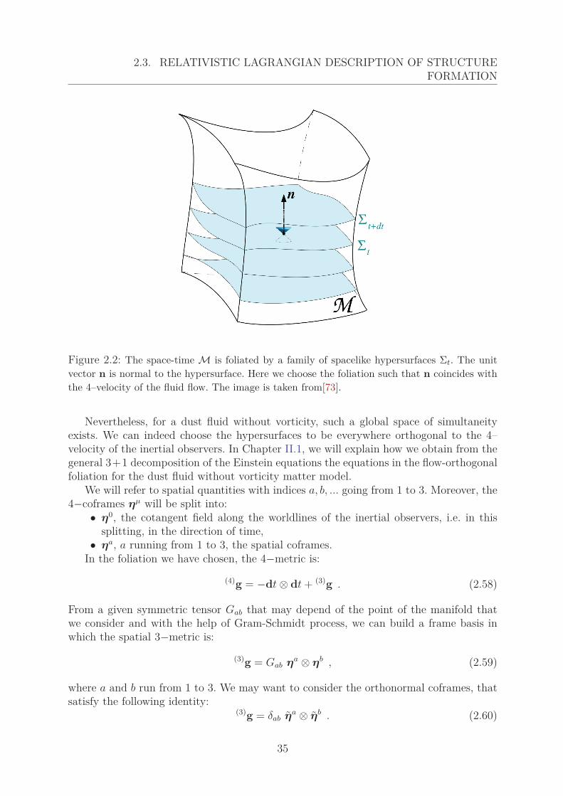
2.3. RELATIVISTIC LAGRANGIAN DESCRIPTION OF STRUCTUREFORMATION
Figure 2.2: The space-time M is foliated by a family of spacelike hypersurfaces Σt. The unitvector n is normal to the hypersurface. Here we choose the foliation such that n coincides withthe 4–velocity of the fluid flow. The image is taken from[73].
Nevertheless, for a dust fluid without vorticity, such a global space of simultaneityexists. We can indeed choose the hypersurfaces to be everywhere orthogonal to the 4–velocity of the inertial observers. In Chapter II.1, we will explain how we obtain from thegeneral 3+1 decomposition of the Einstein equations the equations in the flow-orthogonalfoliation for the dust fluid without vorticity matter model.
We will refer to spatial quantities with indices a, b, ... going from 1 to 3. Moreover, the4−coframes ημ will be split into:
• η0, the cotangent field along the worldlines of the inertial observers, i.e. in thissplitting, in the direction of time,
• ηa, a running from 1 to 3, the spatial coframes.In the foliation we have chosen, the 4−metric is:
(4)g = −dt ⊗ dt + (3)g . (2.58)
From a given symmetric tensor Gab that may depend of the point of the manifold thatwe consider and with the help of Gram-Schmidt process, we can build a frame basis inwhich the spatial 3−metric is:
(3)g = Gab ηa ⊗ ηb , (2.59)
where a and b run from 1 to 3. We may want to consider the orthonormal coframes, thatsatisfy the following identity:
(3)g = δab ηa ⊗ ηb . (2.60)
35
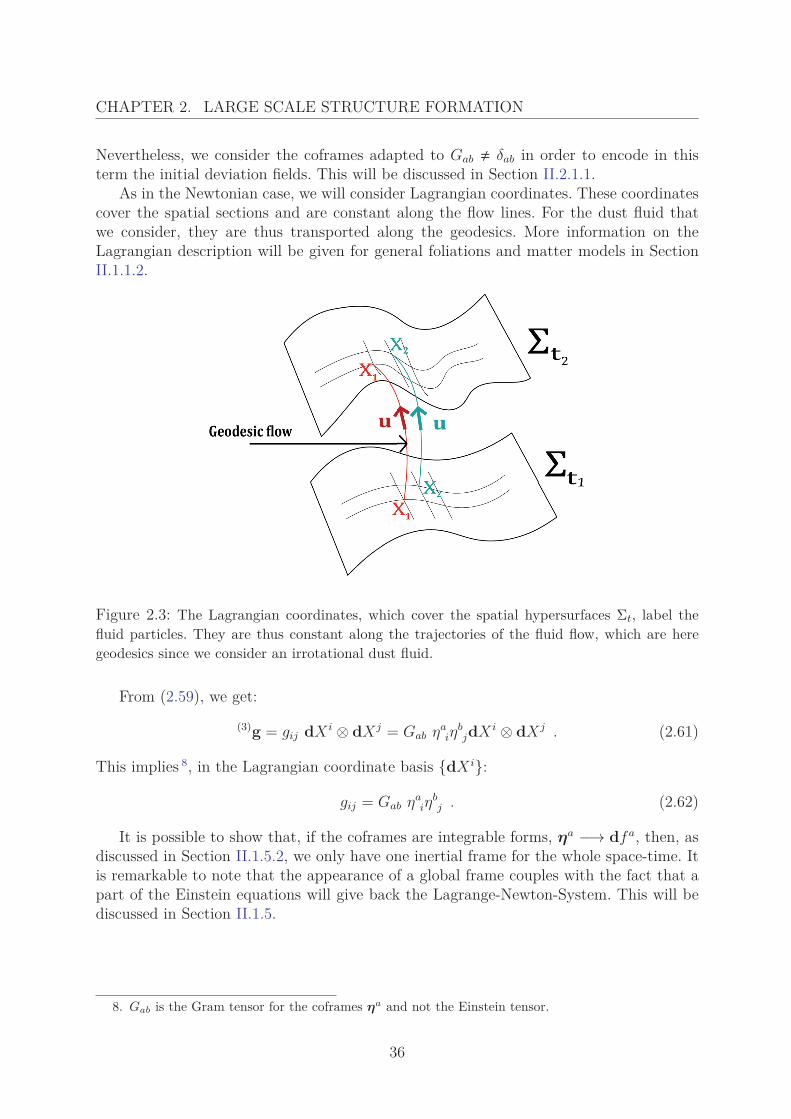
CHAPTER 2. LARGE SCALE STRUCTURE FORMATION
Nevertheless, we consider the coframes adapted to Gab � δab in order to encode in thisterm the initial deviation fields. This will be discussed in Section II.2.1.1.
As in the Newtonian case, we will consider Lagrangian coordinates. These coordinatescover the spatial sections and are constant along the flow lines. For the dust fluid thatwe consider, they are thus transported along the geodesics. More information on theLagrangian description will be given for general foliations and matter models in SectionII.1.1.2.
Figure 2.3: The Lagrangian coordinates, which cover the spatial hypersurfaces Σt, label thefluid particles. They are thus constant along the trajectories of the fluid flow, which are heregeodesics since we consider an irrotational dust fluid.
From (2.59), we get:
(3)g = gij dX i ⊗ dXj = Gab ηaiη
bjdX i ⊗ dXj . (2.61)
This implies 8, in the Lagrangian coordinate basis {dX i}:
gij = Gab ηaiη
bj . (2.62)
It is possible to show that, if the coframes are integrable forms, ηa −→ dfa, then, asdiscussed in Section II.1.5.2, we only have one inertial frame for the whole space-time. Itis remarkable to note that the appearance of a global frame couples with the fact that apart of the Einstein equations will give back the Lagrange-Newton-System. This will bediscussed in Section II.1.5.
8. Gab is the Gram tensor for the coframes ηa and not the Einstein tensor.
36
Chapter 3
Inhomogeneous Cosmology
Contents3.1 Inhomogeneities and their consequences on the global dy-
namics . . . . . . . . . . . . . . . . . . . . . . . . . . . . . . . . . 383.1.1 Hierarchical structures and their density contrast . . . . . . . . 383.1.2 A first insight into averaging and backreaction . . . . . . . . . 39
3.2 Backreaction and spatial average of the Einstein equations . 393.2.1 Einstein equations in the 3 + 1 formalism . . . . . . . . . . . . 403.2.2 Dynamics of a compact domain from the averaged Einstein
equations . . . . . . . . . . . . . . . . . . . . . . . . . . . . . . 41Averaging scalars . . . . . . . . . . . . . . . . . . . . . . . . . . 41Averaging scalar equations: Buchert’s equations . . . . . . . . . 42
3.3 Can backreaction replace Dark Matter and Dark Energy? . . 43
37
The SMC is based on the cosmological principle: global homogeneity and isotropy.But, as it assumes that the average Universe is described by a homogeneous and isotropicmodel, it implies that global and local dynamics are decoupled. This assertion goes farbeyond the cosmological principle.
In this chapter, we first show that for most of the interesting scales, the Universe isnot homogeneous. Taking into account these inhomogeneities will lead, both in Newto-nian gravity and in General Relativity, to an additional term contributing to the globaldynamics of the Universe. Nevertheless, in the Newtonian case, inhomogeneities have noimpact on the global dynamics.
We will consider the relativistic case and explain how the non-linearity of the Einsteinequations results in a difference between the dynamics of an initially averaged space-timeand the averaged dynamics of space-time. The backreaction term quantifies this difference.Afterwards, we will consider the Einstein equations in the 3 + 1 foliation. The averagingprocess that will be introduced is the accurate formalism to determine the impact ofthe inhomogeneities of the matter distribution on the evolution of the Universe. Onceaveraged, the Einstein equations will be analogous to the ones of the SMC , except forthe additional backreaction term, that will encode the coupling of the evolution of thefluid to the geometry of space-time. Finally, we will discuss how the backreaction mayreplace the dark matter and dark energy that the SMC needs to be self-consistent.
3.1 Inhomogeneities and their consequences on theglobal dynamics
Our galaxy is at the edge of a local void in a filamentary sheet [149] that joins us toVirgo Cluster. Furthermore, some surveys estimate that 40 to 50 % of the volume of theUniverse is contained in voids of diameter 30 h−1 Mpc [79, 80]. Nevertheless, the SMCassumes that the averaged Universe can be described by a homogeneous and isotropicmodel. Are the inhomogeneities really negligible? If so, above which scale can we neglectthem?
3.1.1 Hierarchical structures and their density contrastThe density contrast within structures is the dimensionless excess density over the
mean density : δ := (ρ − ρ)/ρ. Its volume average increases as we consider smaller scalesin the Universe:
— for a region of about 10 Mpc, 〈δ〉 � 1 ,— for a typical rich cluster of galaxies, 〈δ〉 � 10 ,— for a galaxy, 〈δ〉 � 105 ,— for a star, 〈δ〉 � 1028 .Nevertheless, the cosmological principle asserts that there exists a spatial length, lying
somewhere between 100 h−1 Mpc and 700 h−1 Mpc, beyond which the Universe is statis-tically homogeneous and isotropic as discussed in Section I.1.2.1. The next step consistsin assuming that this homogeneity and isotropy at large scales allows us to describe theUniverse at these scales with the FLRW metric tensor (1.4). This assumption decouples
38
3.2. BACKREACTION AND SPATIAL AVERAGE OF THE EINSTEINEQUATIONS
the local dynamics from the global dynamics. Nevertheless, we cannot neglect the globalcontribution of inhomogeneities on the dynamics of the averaged space-time [103, 102].
3.1.2 A first insight into averaging and backreactionWe consider the physical space-time described by (M, gμν) and an averaged space-
time (〈M〉 , 〈gμν〉), where we did not specify the averaging procedure 〈·〉. The averagedEinstein equations (1.3) are then:
〈Gμν〉 = 8 π G 〈Tμν〉 , 〈Gμν〉 = 〈Rμν〉 − 12 〈R gμν〉 + Λ 〈gμν〉 . (3.1)
In the same spirit as perturbation theory, we decompose the metric tensor as average anddeviations from the average:
gμν = gμν + δgμν , (3.2)where we have denoted 〈gμν〉 by gμν . We remark that if we do the same thing for gμν , i.e.
gμν = gμν + hμν , (3.3)
then gμν � 〈gμν〉 and hμν � δgμν . We denote by X all the geometrical quantities buildfrom gμν , that caracterize 〈M〉.
Averaged Einstein equations can be reformulated in the following way [65]:
〈Gμν〉 = Gμν + ΔGμν = 8 π G 〈Tμν〉 . (3.4)
Einstein’s theory is non-linear. Thus the averaging process and the construction of theEinstein tensor do not commute. The averaged dynamics of space-time is not equal tothe dynamics of the averaged space-time. This is nevertheless what the standard modelassumes when stating that Einstein’s equations on 〈M〉 are:
Gμν = 8 π G 〈Tμν〉 . (3.5)
ΔGμν , the backreaction term, will be non-zero as long as the inhomogeneities in thephysical space can act on the dynamics of the averaged space-time. The open questionis to understand if this term is big enough to account for dark energy and dark matter.The standard model of cosmology, by neglecting this term, assumes that the dynamics ofstructures at small scales do not influence the global dynamics, at scales larger then thehomogeneity scale.
3.2 Backreaction and spatial average of the Einsteinequations
In the last section, we had a first insight in the origins of backreaction. We will herework with the 3 + 1 formulation of the Einstein equations, first obtained by [6] and thatwe will determine in Chapter II.1. Then, we will give a definition for the spatial averagingoperation we consider. When compared with the equations of the standard model, the
39
CHAPTER 3. INHOMOGENEOUS COSMOLOGY
averaged inhomogeneous Einstein equations exhibit an additional term, the backreaction.It is the sum of two terms, the first being linked to the shear, the vorticity and theexpansion rate of the fluid while the second is the curvature term.
We are looking for a covariant averaging process for tensors in order to preserve thecovariance of Einstein’s equations. Nevertheless, this averaging procedure has not yet beenfound and seems to involve a complex hierarchy of averaging processes [158, 43, 65], thatgoes beyond the two scale model proposed by Zalaletdinov [160]. A way to avoid thisdifficulty is to only average scalar fields and not tensors. Therefore, we will not considerthe averaged Einstein equations in their tensorial form but rather the scalar equationsthat they contain 1.
In the following sections, we present the 3+1 decomposition of the Einstein equations.Then, we define the averaging operation on scalar fields for any spatial domain. Thereafter,we build the averaged evolution equations of an inhomogeneous universe, according toBuchert’s formalism.
3.2.1 Einstein equations in the 3 + 1 formalismAs we will discuss in detail in Section II.1.1.1, the irrotational dust fluid matter model
has the following stress-energy tensor:
Tμν = ρ uμuν , (3.6)
where the 4–velocity is normalized: uμuμ = −1. We choose a flow orthonormal foliation:the hypersurfaces of constant time Σt are normal to the 4–velocity of the fluid flow u. Then,the 4–metric and the 4–velocity have the following form in the Lagrangian coordinatebasis 2, also called Gaussian normal coordinate basis {dX i}:
gμν = diag(−1, gij) ; uμ = (−1, 0) ; uμ = (1, 0) , (3.7)
where gij is the metric on the hypersurface. The 4-dimensional line element in thesecoordinates is:
ds2 = −dt2 + gij dX idXj . (3.8)In the special foliation that we considered for the irrotational dust fluid, the Einstein
equations and the conservation equation can be expressed in terms of the expansiontensor 3, which is a symmetric spatial tensor:
Θij = 13θδij + σij where σij = Θ(ij) − 1
3θδij . (3.10)
1. The resulting averaged Einstein’s equations will only cover the full dynamical degrees of freedomin the case of locally rotationally symmetric spacetimes. In fact, in that case, Einstein’s equations can befully reduced to the dynamics of their covariant scalars [67].
2. The Strong Lagrangian description will be introduced in Section II.1.1.2.3. The expansion tensor is initially a 4–dimensional object, defined by:
Θμν := fαμfβ
ν∇β uα , (3.9)
where fαμ is the projector on the rest-frames of the fluid, defined by (1.16), and ∇β denotes the
4–dimensional covariant derivative.
40
3.2. BACKREACTION AND SPATIAL AVERAGE OF THE EINSTEINEQUATIONS
θ is the trace of Θij, i.e. the expansion rate and σij is the shear. Then, the conservationof the stress-energy tensor reads:
ρ + θρ = 0 . (3.11)
The full projection of the Einstein equations onto the hypersurfaces Σt gives the evolutionequation of the extrinsic curvature:
Θij + θΘi
j = (4πGρ + Λ)δij − Ri
j . (3.12)
The full projection perpendicular to the hypersurface (i.e. along the 4–velocity field) givesthe Hamilton constraint:
R + θ2 − ΘijΘ
ji = 16πGρ + 2Λ . (3.13)
The mixed projection gives the momentum constraint equation:
θ|i − Θji‖j = 0 . (3.14)
The details of the derivation of these equations will be given in Section II.1.1.3. Fromthese equations, we will extract some scalar equations, which will be averaged in SectionI.3.2.2.
3.2.2 Dynamics of a compact domain from the averaged Ein-stein equations
We here define the averaging operator on scalar fields for any domain. This operatorwill enable us to obtain the averaged scalar Einstein equations for the averaged evolutionof an inhomogeneous universe [29].
Averaging scalars
We consider a compact and simply connected domain in the spatial hypersurfaces Σ.This domain D will follow the fluid during its evolution: it will follow the flow lines of thefluid elements. The total rest-mass of the fluid contained in the domain will be conserved.We use Lagrangian coordinates to parametrize the position on Σt.
〈φ〉D (t) := 1VD
∫D
φ(t, X)√
g(t, X) d3X , (3.15)
VD :=∫
D
√g(t, X) d3X , (3.16)
is the volume of the domain and g is the determinant of the spatial metric tensor gij.Lagrangian coordinates index each particle of fluid and are thus comoving with the fluid.Furthermore, with these definitions, we can show that
〈θ〉D = VDVD
. (3.17)
41
CHAPTER 3. INHOMOGENEOUS COSMOLOGY
Finally, from these definitions and identities, we get the non-commutation rule:
〈φ〉D −⟨φ⟩
D = 〈θ〉D 〈φ〉D − 〈θ φ〉D . (3.18)
We conclude that spatial averaging and time evolution do not commute. In the standardapproach, the fluctuations of the CMB are averaged out to obtain the FLRW metric. Thisaveraged universe is then evolved in time. According to (3.18), this is not equivalent to firstevolving the inhomogeneous fields until present time and then spatially averaging them toobtain their final averaged values e.g. averaged density field or cosmological parameters.
Averaging scalar equations: Buchert’s equations
We consider the following three scalar equations. The Hamilton constraint equation(3.19) can be rewritten:
13θ2 = 8πGρ − 1
2R + σ2 + Λ , (3.19)
where σ2 = 12σijσ
ij. The Raychaudhuri equation is obtained by replacing the Ricci scalarin the Hamilton constraint by its expression obtained by the trace of (3.12),
θ = −4πGρ + Λ + 13θ2 − 2σ2 . (3.20)
The last scalar equation we consider is the conservation of mass (3.11). We define theaveraged scale factor
aD(t) =(
VDVDi
)1/3
, (3.21)
Di represents the initial domain and aD(t) is linked to the averaged expansion rate ac-cording to
〈θ〉D = 3 aDaD
. (3.22)
The Buchert’s equations are obtained by combining (3.18) and (3.22) to average (3.19),(3.20) and (3.11):
3(
aDaD
)2= 8πG 〈ρ〉D − 1
2 (RD + QD) + Λ , (3.23)
3 aDaD
= −4πG 〈ρ〉D + QD + Λ , (3.24)
〈ρ〉D + 3 aDaD
〈ρ〉D = 0 , (3.25)
where we have defined
RD := 〈R〉D , QD := 23⟨(θ − 〈θ〉D)2
⟩D − 2
⟨σ2⟩
D . (3.26)
42
3.3. CAN BACKREACTION REPLACE DARK MATTER AND DARK ENERGY?
QD is the kinematical backreaction. The time-derivative of the averaged Hamiltonianconstraint (3.23) is equal to the averaged Raychaudhuri equation (3.24) if the followingintegrability condition is satisfied:
1a6
D
(QD a6
D)˙+ 1
a2D
(RD a2
D)˙ = 0 . (3.27)
This equation has no Newtonian analogue and states that the averaged intrinsic andextrinsic curvature are dynamically coupled.
3.3 Can backreaction replace Dark Matter and DarkEnergy?
To be self-consistent, the SMC has to assume a large amount of dark sources, namelyDark Matter and Dark Energy. The averaged Einstein equations for an inhomogeneousuniverse are analogous to the ones of the SMC but exhibit an additional term: QD, calledbackreaction, that has an impact on the dynamics of the domain considered D. From(3.24), we conclude that
• if QD > 0, it contributes to the acceleration of the expansion of the domain andbehaves like dark energy.
• if QD < 0, it will slow down the expansion of the domain and thus behave likedark matter.
Furthermore, the backreaction behaves like Dark Matter on the small scales and likeDark Energy on the large scales [154]. Moreover, it has been shown that, for an LTBmodel [139], backreaction can mimic the cosmological constant. Nevertheless, a preciseevaluation of the backreaction has still to be achieved for more general inhomogeneousdensity profiles. Finally, the observational data should be entirely reinterpreted in theframework of inhomogeneous cosmology [43] in order to be fully consistent with thisapproach. A complete discussion of the effects of the inhomogeneities on the dynamics ofthe Universe can be found in the following reviews [65, 34, 91, 123, 158].
43
Part II
Insight into General Relativity viaElectromagnetism
Analogy
44

Chapter 1
Gravitoelectromagnetism andGravitoelectric Part of the EinsteinEquations
Contents1.1 Preparatory remarks: 3 + 1 decomposition of the Einstein
equations . . . . . . . . . . . . . . . . . . . . . . . . . . . . . . . 481.1.1 Description of the fluid flow and foliation of space-time . . . . 48
3 + 1 foliation of space-time and description of the fluid flow . 48Stress-energy tensor for the general foliation . . . . . . . . . . . 51
1.1.2 Lagrangian descriptions . . . . . . . . . . . . . . . . . . . . . . 521.1.3 3 + 1 decomposition of the Einstein equations . . . . . . . . . . 531.1.4 Lagrangian formulation of Einstein’s equations for an irrota-
tional dust fluid matter model . . . . . . . . . . . . . . . . . . 541.2 Historical introduction to GEM . . . . . . . . . . . . . . . . . . 571.3 Maxwellian formulation of the Euler-Newton-System . . . . . 58
Scalar and vector potentials of the current density . . . . . . . 59Kinematical intuition for the vector potential . . . . . . . . . . 59Lorentz–covariant generalization of Newton’s theory . . . . . . 59
1.4 Decomposition of the Weyl tensor and Maxwell-Weyl equa-tions . . . . . . . . . . . . . . . . . . . . . . . . . . . . . . . . . . 61
1.4.1 Newtonian dynamics, tidal tensor and relativistic generalization 611.4.2 Electric and magnetic parts of the Weyl tensor . . . . . . . . . 621.4.3 Maxwell-Weyl equations . . . . . . . . . . . . . . . . . . . . . . 631.4.4 Newtonian limit of the electric and magnetic parts . . . . . . . 65
1.5 Gravitoelectric part of the Einstein equations and the L-N-S 661.5.1 Gravitoelectric part of the Einstein equations . . . . . . . . . . 661.5.2 Minkowski Restriction of the gravitoelectric system . . . . . . . 67
Definition of the Minkowski Restriction . . . . . . . . . . . . . 67Equivalence of the integrability of the orthonormal and adapted
coframes and the flatness of space . . . . . . . . . . . 67
46
Minkowski Restriction of the gravitoelectric part of the Einsteinequations . . . . . . . . . . . . . . . . . . . . . . . . . 68
1.5.3 Minkowski Restriction of the other Einstein equations . . . . . 691.6 Concluding remarks . . . . . . . . . . . . . . . . . . . . . . . . . 70
47
Gravitoelectromagnetism is an analogy between the equations of Newtonian or rela-tivistic gravity and electromagnetism. This approach of gravity allows a special under-standing of Einstein’s theory of General Relativity. In this chapter, we will give a briefhistorical presentation of the development of this analogy and illustrate it in the caseof the Newtonian gravitation theory. Thereafter, we will discuss the formulation of theEinstein equations in terms of the electric and magnetic parts of the Weyl tensor. As wewill see, this formulation exhibits strong similarities with the Maxwell equations. Fur-thermore, we will show that the part of the Einstein equations, namely the gravitoelectricpart, is the non-integrable counterpart of the Lagrange-Newton-System. Exploiting thisformal analogy will be the subject of Chapter II.2, where a relativistic generalization ofthe Newtonian perturbation solutions to order n will be presented. The GEM analogy, aswell as the perturbation scheme that we will discuss in the next chapters, is based on the3+1 decomposition of the Einstein equations. Even if in most of the work that I carriedout during my PhD, we considered the irrotational dust fluid as a matter model for thecontent of the Universe, some results for the perfect fluid matter model will be given inAppendix A.
In this chapter, I first present the general 3 + 1 foliation of space-time and introducethe geometrical quantities that parametrize the foliation. We will explain how these quan-tities can be constrained in order to build a foliation adapted to the fluid flow, namelya comoving synchronous foliation. The Einstein equations will be given in the 3 + 1 de-composition. The extrinsic curvature and expansion tensor will be expressed in terms ofthe physical and geometrical quantities we will define. These general results will then bespecified on the case of the irrotational dust fluid matter model and for the perfect fluidmatter model in Appendix A. Most of the results presented here are discussed in [129].With permission of the authors, I present the following introductory notes here, since mywork is based on some of these non-published results (in particular, appendix A).
1.1 Preparatory remarks: 3 + 1 decomposition of theEinstein equations
1.1.1 Description of the fluid flow and foliation of space-timeIn this section, we explain how we can relate the fluid flow to the foliation of space-
time. Then, we present the general space-time foliations for an arbitrary set of coordinatesand discuss how the degrees of freedom associated to the choice of the coordinate system,namely the lapse α and the shift β, are related to the physical quantities of the fluidflow. Thereafter, we define the rest-frame of the fluid flow and give the expression of thestress-energy tensor of a perfect fluid in this frame.
3 + 1 foliation of space-time and description of the fluid flow
Fluid flow and hypersurfaces
48
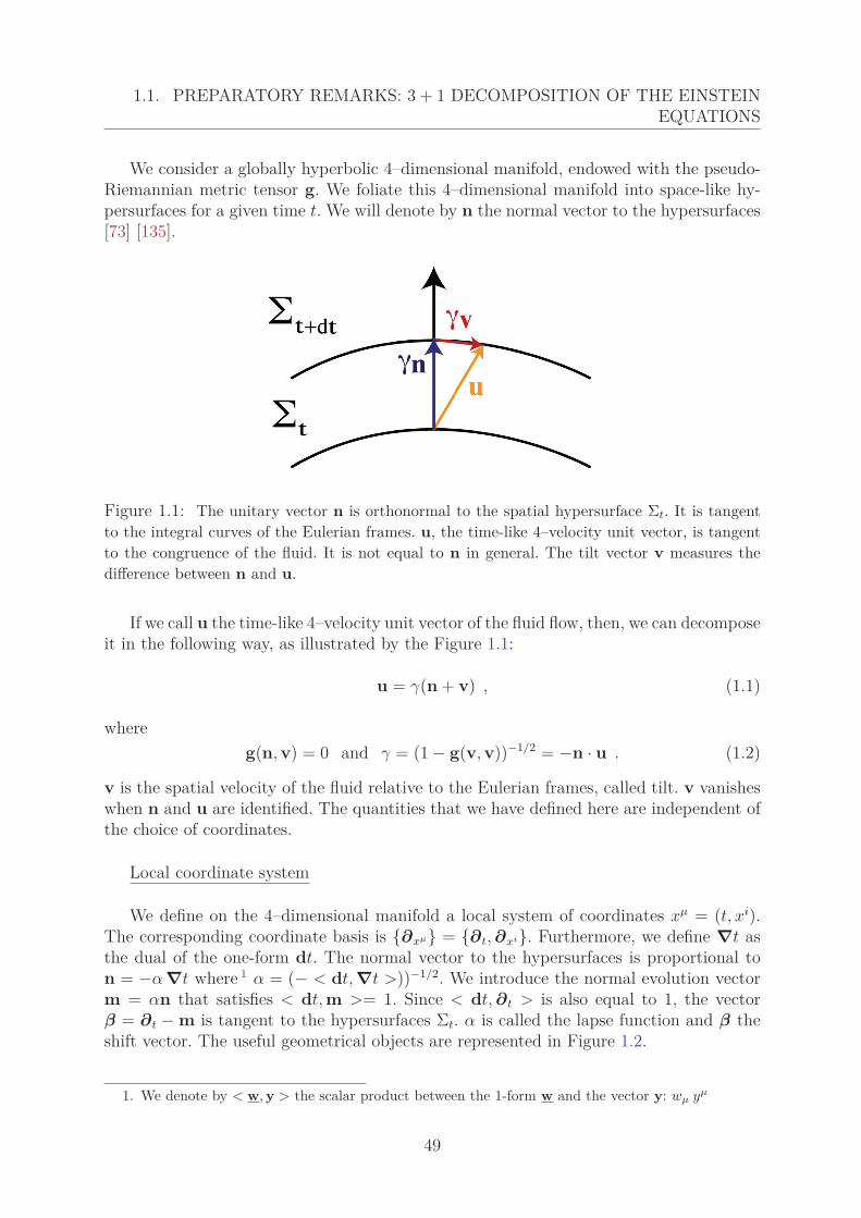
1.1. PREPARATORY REMARKS: 3 + 1 DECOMPOSITION OF THE EINSTEINEQUATIONS
We consider a globally hyperbolic 4–dimensional manifold, endowed with the pseudo-Riemannian metric tensor g. We foliate this 4–dimensional manifold into space-like hy-persurfaces for a given time t. We will denote by n the normal vector to the hypersurfaces[73] [135].
Figure 1.1: The unitary vector n is orthonormal to the spatial hypersurface Σt. It is tangentto the integral curves of the Eulerian frames. u, the time-like 4–velocity unit vector, is tangentto the congruence of the fluid. It is not equal to n in general. The tilt vector v measures thedifference between n and u.
If we call u the time-like 4–velocity unit vector of the fluid flow, then, we can decomposeit in the following way, as illustrated by the Figure 1.1:
u = γ(n + v) , (1.1)
whereg(n, v) = 0 and γ = (1 − g(v, v))−1/2 = −n · u . (1.2)
v is the spatial velocity of the fluid relative to the Eulerian frames, called tilt. v vanisheswhen n and u are identified. The quantities that we have defined here are independent ofthe choice of coordinates.
Local coordinate system
We define on the 4–dimensional manifold a local system of coordinates xμ = (t, xi).The corresponding coordinate basis is {∂xμ} = {∂t, ∂xi}. Furthermore, we define ∇t asthe dual of the one-form dt. The normal vector to the hypersurfaces is proportional ton = −α ∇t where 1 α = (− < dt, ∇t >))−1/2. We introduce the normal evolution vectorm = αn that satisfies < dt, m >= 1. Since < dt, ∂t > is also equal to 1, the vectorβ = ∂t − m is tangent to the hypersurfaces Σt. α is called the lapse function and β theshift vector. The useful geometrical objects are represented in Figure 1.2.
1. We denote by < w, y > the scalar product between the 1-form w and the vector y: wμ yμ
49
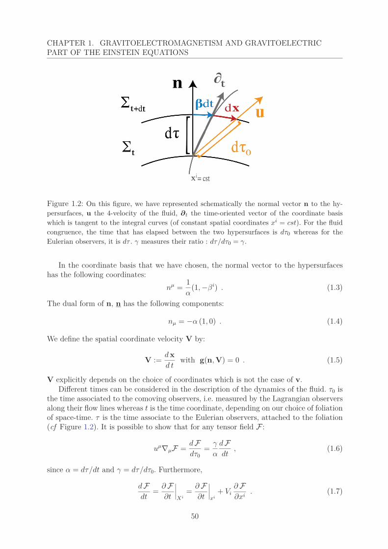
CHAPTER 1. GRAVITOELECTROMAGNETISM AND GRAVITOELECTRICPART OF THE EINSTEIN EQUATIONS
Figure 1.2: On this figure, we have represented schematically the normal vector n to the hy-persurfaces, u the 4-velocity of the fluid, ∂t the time-oriented vector of the coordinate basiswhich is tangent to the integral curves (of constant spatial coordinates xi = cst). For the fluidcongruence, the time that has elapsed between the two hypersurfaces is dτ0 whereas for theEulerian observers, it is dτ . γ measures their ratio : dτ/dτ0 = γ.
In the coordinate basis that we have chosen, the normal vector to the hypersurfaceshas the following coordinates:
nμ = 1α
(1, −βi) . (1.3)
The dual form of n, n has the following components:
nμ = −α (1, 0) . (1.4)
We define the spatial coordinate velocity V by:
V := d xd t
with g(n, V) = 0 . (1.5)
V explicitly depends on the choice of coordinates which is not the case of v.Different times can be considered in the description of the dynamics of the fluid. τ0 is
the time associated to the comoving observers, i.e. measured by the Lagrangian observersalong their flow lines whereas t is the time coordinate, depending on our choice of foliationof space-time. τ is the time associate to the Eulerian observers, attached to the foliation(cf Figure 1.2). It is possible to show that for any tensor field F :
uμ∇μF = d Fdτ0
= γ
α
d Fdt
, (1.6)
since α = dτ/dt and γ = dτ/dτ0. Furthermore,
d Fdt
= ∂ F∂t
∣∣∣∣Xi
= ∂ F∂t
∣∣∣∣xi
+ Vi∂ F∂xi
. (1.7)
50
1.1. PREPARATORY REMARKS: 3 + 1 DECOMPOSITION OF THE EINSTEINEQUATIONS
From now on, we will denote d Fdτ0
by F .Furthermore, for d λ = βdt + dx, we show the useful equality:
v = d λ
dτ= dt
dτ(V + β) = 1
α(V + β) . (1.8)
For (1.1) and (1.8) we conclude that the 4–velocity of the fluid can be expressed as:
u = γ
α(αn + β + V) . (1.9)
Thus, the components of the fluid flow vector and its dual are:
uμ = γ
α
(1, V i
), uμ = γ
α
(−α2 + βk(βk + Vk), βi + Vi
). (1.10)
If we define the projector on the spatial hypersurfaces as:
hμν = gμν + nμnν , (1.11)
it satisfies the following equalities:
hμνnμ = 0 , hμα hα
ν = hμν , hμνhμν = 3 . (1.12)
The components of the metric on the coordinate basis are:
gμν =(
−α2 + βkβk βj
βi hij
); gμν =
(− 1
α2βj
α2βi
α2 hij − βiβj
α2
). (1.13)
Thus, the 4–dimensional line element can be decomposed as:
ds2 = gμνdxμdxν = −(α2 − βkβk)dt2 + βidt dxi + hijdxidxj . (1.14)
Stress-energy tensor for the general foliation
In the rest-frame of the fluid, the stress-energy tensor for a general matter model canbe decomposed relative to the 4–velocity u as:
Tμν = ε uμuν + qμuν + qνuμ + p fμν + πμν , (1.15)
where ε is the relativistic energy density, qμ the relativistic momentum density, p theisotropic pressure, πμν the trace-free anisotropic pressure. We have defined the projectoron the rest-frames of the fluid:
fμν = gμν + uμuν , (1.16)
which satisfies the following equalities:
fμνuμ = 0 , fμα fα
ν = fμν , fμνfμν = 3 . (1.17)
In the rest-frame of the fluid, the stress-energy tensor of the perfect fluid is obtained forqμ = πμν = 0:
Tμν = ε uμuν + p fμν . (1.18)
51
CHAPTER 1. GRAVITOELECTROMAGNETISM AND GRAVITOELECTRICPART OF THE EINSTEIN EQUATIONS
Furthermore, for pressure-free matter, called dust matter model (which is the one usedto model the Cold Dark Matter), the stress-energy tensor becomes:
T dustμν = ε uμuν . (1.19)
The stress-energy tensor for general matter models can also be described in this foliationusing a foliation-dependent decomposition:
Tμν = E nμnν + 2 n(μJν) + Sμν , (1.20)
where E, the energy density, Jμ the momentum density and Sμν the stress density, are allevaluated in the Eulerian frames i.e. the ones transported along the integral curves of n:
E = nαnβ Tαβ , Jν = −hαμnβTαβ , Sμν = hα
μhβνTαβ . (1.21)
For a perfect fluid matter model, the energy density, the momentum density and the stressdensity evaluated in the Eulerian frames can be expressed as functions of ε the relativisticenergy and the pressure p:
E = γ2ε + (γ2 − 1)p , Jμ = γ2
α(ε + p)(βμ + Vμ) , (1.22)
Sμν = γ2
α2 (ε + p)(βμ + Vμ)(βν + Vν) + p hμν , (1.23)
S = (γ2 − 1)ε + (γ2 + 2)p . (1.24)Now that we have built all the quantities needed to describe both the fluid flow andthe geometry of space sections, we are able to formulate the Einstein equations for this3 + 1 foliation of space-time. But before, we present the relativistic generalization of theLagrangian description.
1.1.2 Lagrangian descriptionsWe here generalize the Newtonian notion of Lagrangian description and introduce two
Lagrangian descriptions: the Weak and the Strong descriptions, for which the observerfollows the fluid flow. The Weak Lagrangian description of the fluid is obtained for a shiftvector β attached to the fluid flow and the coordinate velocity is then zero:
β = α v ⇔ V = 0 . (1.25)
Furthermore, if the lapse function is equal to the Lorentz factor, α = γ, then thehypersurfaces of constant t are also hypersurfaces of constant fluid proper time τ0. Thisdescription is the Strong Lagrangian description. The two Lagrangian descriptions con-sider spatial Lagrangian coordinates (cf Section I.2.2.1) and provide us with a relativisticgeneralization of the Newtonian Lagrangian formalism.
The 4–velocity can then be expressed as:
uμ = (1, 0) and uμ = (−1, β) . (1.26)
52
1.1. PREPARATORY REMARKS: 3 + 1 DECOMPOSITION OF THE EINSTEINEQUATIONS
The Strong Lagrangian description thus defines a comoving synchronous slicing of space-time. From (1.6), we can show that in this description for any tensor field F ,
d Fdt
= ∂ F∂t
∣∣∣∣Xi
= d Fdτ0
, (1.27)
i.e. all the time derivatives are equal.Since the Lorentz factor γ and the shift α are equal, from (1.2) we conclude that
γ =(1 − βkβk
α2
)−1/2and therefore we obtain the equality:
α2 − βkβk = 1 . (1.28)
This equality, which is a scalar constraint connecting the lapse and the shift, was discussedby H. Asada and M. Kasai 2 in [7].
1.1.3 3 + 1 decomposition of the Einstein equationsWe here determine the 3 + 1 decomposition of the Einstein equations in terms of the
kinematical and geometrical quantities that we introduced in last section. We project theRicci curvature tensor and the stress-energy tensor either on the normal vector to thehypersurfaces n or on the tangent space Σt [73] [73] [135].
The full projection of the Einstein equations on the spatial hypersurface Σt gives theevolution equation for the extrinsic curvature:
∂t|xiKij = α
(Ri
j + KKij − δi
jΛ + 4πG[(S − E)δij] − Si
j
)−α
|i|j + βkKi
j |k + Kikβk |j − Kk
jβi|k ,
(1.29)
where Kij = −hα
i hβj ∇α nβ is the extrinsic curvature tensor of the hypersurface, ∇α is the
four-covariant derivative. ‖i is the three-covariant derivative and |i is the simple three-derivative equal to ∂xi . ∂t|xi is the time derivative along the integral curves, for which thecoordinates xi are held fixed.
The full projection along n gives the Hamilton constraint:
R + K2 − KijKj
i = 16πGE + 2Λ . (1.30)
while the mixed projectionKk
j |k − K|i = 8πGJi , (1.31)gives the momentum constraint.
With the lapse function α and the shift vector β that we defined in last section, weexpress the extrinsic curvature Ki
j in terms of metric [73]:
∂t|xihij = −2αKij + 2β(i‖j) . (1.32)
2. H. Asada and M. Kasai took another convention for the metric signature: (+, −, −, −). They there-fore get α2 − βkβk = −1 instead of α2 − βkβk = 1.
53
CHAPTER 1. GRAVITOELECTROMAGNETISM AND GRAVITOELECTRICPART OF THE EINSTEIN EQUATIONS
From equation (1.7) and (1.32), we obtain:
Kij = 1
2
(1α
(V lhikhkj|l + βi‖j + β
‖ij ) − hikhkj
γ
), (1.33)
its trace being
K = 12
(1α
(V lhikhkj|l + 2β‖i
i ) − hikhki
γ
). (1.34)
(1.33) and (1.34) can be inserted into (1.29), (1.31) and (1.30) to obtain the evolutionequations for the geometry of the spatial hypersurfaces. In the Strong Lagrangian descrip-tion, these expressions become:
Kij = 1
2α
(−hikhkj + βi
‖j + β‖i
j
); K = 1
2α
(−hikhki + 2β
‖ii
). (1.35)
The four-covariant derivative of u contains the kinematical information of the fluidflow. We consider the spatial components of the projection onto the hypersurfaces of the4–velocity gradient ∇ν uμ:
Lij := hμih
νj ∇ν uμ = Θij + ωij − ujai = ui|j − Γα
ij uα . (1.36)
ai is the acceleration: ai := uμ∇μ ui , Θij is the expansion tensor, θ its trace, also calledexpansion rate. σij is the symmetric traceless part of Θij and is called the shear tensorwhile ωij is the vorticity of the fluid. In terms of the quantities that we defined, we get:
Lij = γ
α(βi + Vi)‖j − γ
α3
(−α2 + βkβk + βkVk
)(12
∂
∂t
∣∣∣∣Xi
hij − β(i‖j)
). (1.37)
With condition (1.28), in the Strong Lagrangian description, Lij becomes :
Lij = hij
2α2 + (1 − 1α2 )β(i‖j) + β[i|j] . (1.38)
We here derived the 3 + 1 decomposition of the Einstein equations for a general mattermodel in the Strong Lagrangian description. Now, we will determine what these equationsbecome for the dust matter model. We will express these equations in terms of the Cartancoframes, that were defined in Section I.2.3.2. As we have seen, the Cartan coframes canindeed be connected to the spatial metric by (2.59).
1.1.4 Lagrangian formulation of Einstein’s equations for an ir-rotational dust fluid matter model
Since we consider an irrotational flow, it is possible to choose a foliation for which thenormal vector n coincides with the 4–velocity u of the fluid flow 3. In such a foliation,
3. If the fluid flow has vorticity, the local rest-frames do not form a global hypersurface. A 3 + 1foliation for which n = u cannot be built. The description of a non–zero vorticity will indeed require a1 + 3 threading of spacetime [68].
54
1.1. PREPARATORY REMARKS: 3 + 1 DECOMPOSITION OF THE EINSTEINEQUATIONS
the acceleration vanishes since the trajectories are geodesics and, furthermore, γ = 1.Moreover, if we consider the Strong Lagrangian description, then
β = 0 ; α = 1 . (1.39)
Θij, the expansion tensor, and Kij, the extrinsic curvature tensor, have now the followingform:
Θij = gij
2 ; Kij = −Θij = − gij
2 , (1.40)
where we now use the notation gij instead of hij. Furthermore, we now also have hij = gij
in this foliation.As was shown in [35], we now insert the expression of the metric in terms of the Cartan
coframes (2.59) and (2.62) into the Einstein equations to obtain the following system ofequations, called the Lagrange-Einstein-System:
Gab ηa[iη
bj] = 0 ; (1.41)
12J
εabcεikl(ηa
jηbkηc
l
)˙ = −Ri
j + (4πG + Λ) δij ; (1.42)
12J
εabcεmjkηa
mηbjη
ck = −R
2 + (8πG + Λ) ; (1.43)(εabcε
iklηajη
bkηc
l
)||i =
(εabcε
iklηaiη
bkηc
l
)|j , (1.44)
The system {(1.41)− (1.44)} consists of 13 equations. The equations are, respectively, thesymmetry of the metric (1.41) (3 equations), the equation of motion (1.42) (i.e. the evo-lution equation for the extrinsic curvature) (6 equations), the energy constraint (1.43) (1equation) and the momentum constraints (1.44) (3 equations). Thus, the first 9 equationsfurnish evolution equations for the 9 coefficient functions of the 3 Cartan coframe fields.
The double vertical slash denotes the covariant spatial derivative with respect to the3–metric and the spatial connection is assumed to be symmetric. The first equation canbe replaced by the irrotationality condition:
Gab ηa[iη
bj] = 0 . (1.45)
Furthermore, the trace of the equation of motion and the energy constraint leads to theRaychaudhuri equation:
12J
εabcεik�ηa
iηbkηc
� = Λ − 4πG . (1.46)
The above system is equivalent to the results developed in [35] in a different coframebasis: in the first paper the choice of the standard orthonormal coframes has been made,whereas, from [36] on, the choice of the adapted coframes is preferred because it allows aformally closer Newtonian analogy.
The Lagrange-Einstein-System can also be expressed in a coordinate-independent way,using differential geometry (cf Section I.2.3.1). We then obtain the following set of equa-
55
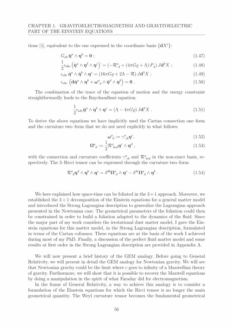
CHAPTER 1. GRAVITOELECTROMAGNETISM AND GRAVITOELECTRICPART OF THE EINSTEIN EQUATIONS
tions [4], equivalent to the one expressed in the coordinate basis {dX i}:
Gab ηa ∧ ηb = 0 ; (1.47)12εdbc
(ηa ∧ ηb ∧ ηc
)˙ = (−Ra
d + (4πG + Λ) δad) Jd3X ; (1.48)
εabc ηa ∧ ηb ∧ ηc = (16πG + 2Λ − R) Jd3X ; (1.49)εabc
(dηa ∧ ηb + ωa
d ∧ ηd ∧ ηb)
= 0 . (1.50)
The combination of the trace of the equation of motion and the energy constraintstraightforwardly leads to the Raychaudhuri equation:
12εabcη
a ∧ ηb ∧ ηc = (Λ − 4πG) Jd3X . (1.51)
To derive the above equations we have implicitly used the Cartan connection one–formand the curvature two–form that we do not need explicitly in what follows:
ωab := γa
cbηc, (1.52)
Ωad := 1
2Rabcdηc ∧ ηd , (1.53)
with the connection and curvature coefficients γacb and Ra
bcd in the non-exact basis, re-spectively. The 3–Ricci tensor can be expressed through the curvature two–form:
Radηd ∧ ηb ∧ ηc = δdbΩa
d ∧ ηc − δdcΩad ∧ ηb . (1.54)
We here explained how space-time can be foliated in the 3+1 approach. Moreover, weestablished the 3 + 1 decomposition of the Einstein equations for a general matter modeland introduced the Strong Lagrangian description to generalize the Lagrangian approachpresented in the Newtonian case. The geometrical parameters of the foliation could thenbe constrained in order to build a foliation adapted to the dynamics of the fluid. Sincethe major part of my work considers the irrotational dust matter model, I gave the Ein-stein equations for this matter model, in the Strong Lagrangian description, formulatedin terms of the Cartan coframes. These equations are at the basis of the work I achievedduring most of my PhD. Finally, a discussion of the perfect fluid matter model and someresults at first order in the Strong Lagrangian description are provided in Appendix A.
We will now present a brief history of the GEM analogy. Before going to GeneralRelativity, we will present in detail the GEM analogy for Newtonian gravity. We will seethat Newtonian gravity could be the limit where c goes to infinity of a Maxwellian theoryof gravity. Furthermore, we will show that it is possible to recover the Maxwell equationsby doing a manipulation in the spirit of what Faraday did for electromagnetism.
In the frame of General Relativity, a way to achieve this analogy is to consider aformulation of the Einstein equations for which the Ricci tensor is no longer the maingeometrical quantity. The Weyl curvature tensor becomes the fundamental geometrical
56
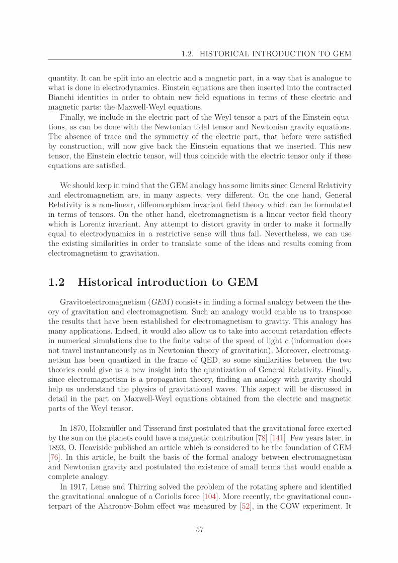
1.2. HISTORICAL INTRODUCTION TO GEM
quantity. It can be split into an electric and a magnetic part, in a way that is analogue towhat is done in electrodynamics. Einstein equations are then inserted into the contractedBianchi identities in order to obtain new field equations in terms of these electric andmagnetic parts: the Maxwell-Weyl equations.
Finally, we include in the electric part of the Weyl tensor a part of the Einstein equa-tions, as can be done with the Newtonian tidal tensor and Newtonian gravity equations.The absence of trace and the symmetry of the electric part, that before were satisfiedby construction, will now give back the Einstein equations that we inserted. This newtensor, the Einstein electric tensor, will thus coincide with the electric tensor only if theseequations are satisfied.
We should keep in mind that the GEM analogy has some limits since General Relativityand electromagnetism are, in many aspects, very different. On the one hand, GeneralRelativity is a non-linear, diffeomorphism invariant field theory which can be formulatedin terms of tensors. On the other hand, electromagnetism is a linear vector field theorywhich is Lorentz invariant. Any attempt to distort gravity in order to make it formallyequal to electrodynamics in a restrictive sense will thus fail. Nevertheless, we can usethe existing similarities in order to translate some of the ideas and results coming fromelectromagnetism to gravitation.
1.2 Historical introduction to GEMGravitoelectromagnetism (GEM) consists in finding a formal analogy between the the-
ory of gravitation and electromagnetism. Such an analogy would enable us to transposethe results that have been established for electromagnetism to gravity. This analogy hasmany applications. Indeed, it would also allow us to take into account retardation effectsin numerical simulations due to the finite value of the speed of light c (information doesnot travel instantaneously as in Newtonian theory of gravitation). Moreover, electromag-netism has been quantized in the frame of QED, so some similarities between the twotheories could give us a new insight into the quantization of General Relativity. Finally,since electromagnetism is a propagation theory, finding an analogy with gravity shouldhelp us understand the physics of gravitational waves. This aspect will be discussed indetail in the part on Maxwell-Weyl equations obtained from the electric and magneticparts of the Weyl tensor.
In 1870, Holzmüller and Tisserand first postulated that the gravitational force exertedby the sun on the planets could have a magnetic contribution [78] [141]. Few years later, in1893, O. Heaviside published an article which is considered to be the foundation of GEM[76]. In this article, he built the basis of the formal analogy between electromagnetismand Newtonian gravity and postulated the existence of small terms that would enable acomplete analogy.
In 1917, Lense and Thirring solved the problem of the rotating sphere and identifiedthe gravitational analogue of a Coriolis force [104]. More recently, the gravitational coun-terpart of the Aharonov-Bohm effect was measured by [52], in the COW experiment. It
57
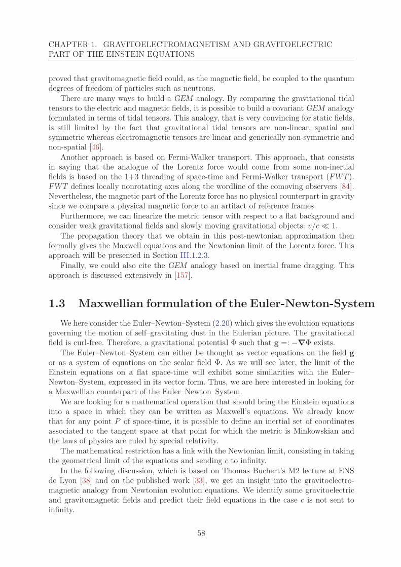
CHAPTER 1. GRAVITOELECTROMAGNETISM AND GRAVITOELECTRICPART OF THE EINSTEIN EQUATIONS
proved that gravitomagnetic field could, as the magnetic field, be coupled to the quantumdegrees of freedom of particles such as neutrons.
There are many ways to build a GEM analogy. By comparing the gravitational tidaltensors to the electric and magnetic fields, it is possible to build a covariant GEM analogyformulated in terms of tidal tensors. This analogy, that is very convincing for static fields,is still limited by the fact that gravitational tidal tensors are non-linear, spatial andsymmetric whereas electromagnetic tensors are linear and generically non-symmetric andnon-spatial [46].
Another approach is based on Fermi-Walker transport. This approach, that consistsin saying that the analogue of the Lorentz force would come from some non-inertialfields is based on the 1+3 threading of space-time and Fermi-Walker transport (FWT).FWT defines locally nonrotating axes along the wordline of the comoving observers [84].Nevertheless, the magnetic part of the Lorentz force has no physical counterpart in gravitysince we compare a physical magnetic force to an artifact of reference frames.
Furthermore, we can linearize the metric tensor with respect to a flat background andconsider weak gravitational fields and slowly moving gravitational objects: v/c � 1.
The propagation theory that we obtain in this post-newtonian approximation thenformally gives the Maxwell equations and the Newtonian limit of the Lorentz force. Thisapproach will be presented in Section III.1.2.3.
Finally, we could also cite the GEM analogy based on inertial frame dragging. Thisapproach is discussed extensively in [157].
1.3 Maxwellian formulation of the Euler-Newton-SystemWe here consider the Euler–Newton–System (2.20) which gives the evolution equations
governing the motion of self–gravitating dust in the Eulerian picture. The gravitationalfield is curl-free. Therefore, a gravitational potential Φ such that g =: −∇Φ exists.
The Euler–Newton–System can either be thought as vector equations on the field gor as a system of equations on the scalar field Φ. As we will see later, the limit of theEinstein equations on a flat space-time will exhibit some similarities with the Euler–Newton–System, expressed in its vector form. Thus, we are here interested in looking fora Maxwellian counterpart of the Euler–Newton–System.
We are looking for a mathematical operation that should bring the Einstein equationsinto a space in which they can be written as Maxwell’s equations. We already knowthat for any point P of space-time, it is possible to define an inertial set of coordinatesassociated to the tangent space at that point for which the metric is Minkowskian andthe laws of physics are ruled by special relativity.
The mathematical restriction has a link with the Newtonian limit, consisting in takingthe geometrical limit of the equations and sending c to infinity.
In the following discussion, which is based on Thomas Buchert’s M2 lecture at ENSde Lyon [38] and on the published work [33], we get an insight into the gravitoelectro-magnetic analogy from Newtonian evolution equations. We identify some gravitoelectricand gravitomagnetic fields and predict their field equations in the case c is not sent toinfinity.
58
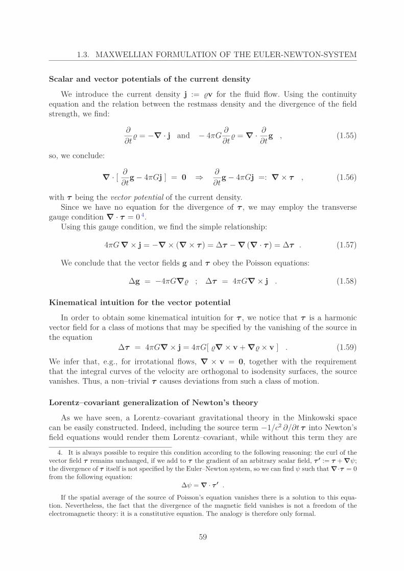
1.3. MAXWELLIAN FORMULATION OF THE EULER-NEWTON-SYSTEM
Scalar and vector potentials of the current density
We introduce the current density j := v for the fluid flow. Using the continuityequation and the relation between the restmass density and the divergence of the fieldstrength, we find:
∂
∂t = −∇ · j and − 4πG
∂
∂t = ∇ · ∂
∂tg , (1.55)
so, we conclude:
∇ · [ ∂
∂tg − 4πGj ] = 0 ⇒ ∂
∂tg − 4πGj =: ∇ × τ , (1.56)
with τ being the vector potential of the current density.Since we have no equation for the divergence of τ , we may employ the transverse
gauge condition ∇ · τ = 0 4.Using this gauge condition, we find the simple relationship:
4πG ∇ × j = −∇ × (∇ × τ ) = Δτ − ∇ (∇ · τ ) = Δτ . (1.57)
We conclude that the vector fields g and τ obey the Poisson equations:
Δg = −4πG∇ ; Δτ = 4πG∇ × j . (1.58)
Kinematical intuition for the vector potential
In order to obtain some kinematical intuition for τ , we notice that τ is a harmonicvector field for a class of motions that may be specified by the vanishing of the source inthe equation
Δτ = 4πG∇ × j = 4πG[ ∇ × v + ∇ × v ] . (1.59)
We infer that, e.g., for irrotational flows, ∇ × v = 0, together with the requirementthat the integral curves of the velocity are orthogonal to isodensity surfaces, the sourcevanishes. Thus, a non–trivial τ causes deviations from such a class of motion.
Lorentz–covariant generalization of Newton’s theory
As we have seen, a Lorentz–covariant gravitational theory in the Minkowski spacecan be easily constructed. Indeed, including the source term −1/c2 ∂/∂t τ into Newton’sfield equations would render them Lorentz–covariant, while without this term they are
4. It is always possible to require this condition according to the following reasoning: the curl of thevector field τ remains unchanged, if we add to τ the gradient of an arbitrary scalar field, τ ′ := τ + ∇ψ;the divergence of τ itself is not specified by the Euler–Newton system, so we can find ψ such that ∇·τ = 0from the following equation:
Δψ = ∇ · τ ′ .
If the spatial average of the source of Poisson’s equation vanishes there is a solution to this equa-tion. Nevertheless, the fact that the divergence of the magnetic field vanishes is not a freedom of theelectromagnetic theory: it is a constitutive equation. The analogy is therefore only formal.
59
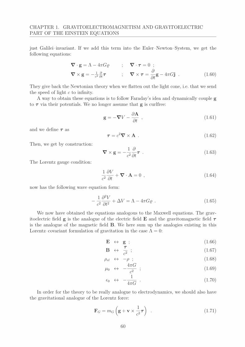
CHAPTER 1. GRAVITOELECTROMAGNETISM AND GRAVITOELECTRICPART OF THE EINSTEIN EQUATIONS
just Galilei–invariant. If we add this term into the Euler–Newton–System, we get thefollowing equations:
∇ · g = Λ − 4πG ; ∇ · τ = 0 ;
∇ × g = − 1c2
∂∂t
τ ; ∇ × τ = ∂
∂tg − 4πGj . (1.60)
They give back the Newtonian theory when we flatten out the light cone, i.e. that we sendthe speed of light c to infinity.
A way to obtain these equations is to follow Faraday’s idea and dynamically couple gto τ via their potentials. We no longer assume that g is curlfree:
g = −∇V − ∂A∂t
, (1.61)
and we define τ asτ = c2∇ × A . (1.62)
Then, we get by construction:∇ × g = − 1
c2∂
∂tτ . (1.63)
The Lorentz gauge condition:
1c2
∂V
∂t+ ∇ · A = 0 , (1.64)
now has the following wave equation form:
− 1c2
∂2V
∂t2 + ΔV = Λ − 4πG . (1.65)
We now have obtained the equations analogous to the Maxwell equations. The grav-itoelectric field g is the analogue of the electric field E and the gravitomagnetic field τis the analogue of the magnetic field B. We here sum up the analogies existing in thisLorentz–covariant formulation of gravitation in the case Λ = 0:
E ↔ g ; (1.66)B ↔ τ
c2 ; (1.67)
ρel ↔ −ρ ; (1.68)
μ0 ↔ −4πG
c2 ; (1.69)
ε0 ↔ − 14πG
. (1.70)
In order for the theory to be really analogue to electrodynamics, we should also havethe gravitational analogue of the Lorentz force:
FG = mG
(g + v × 1
c2 τ)
. (1.71)
60
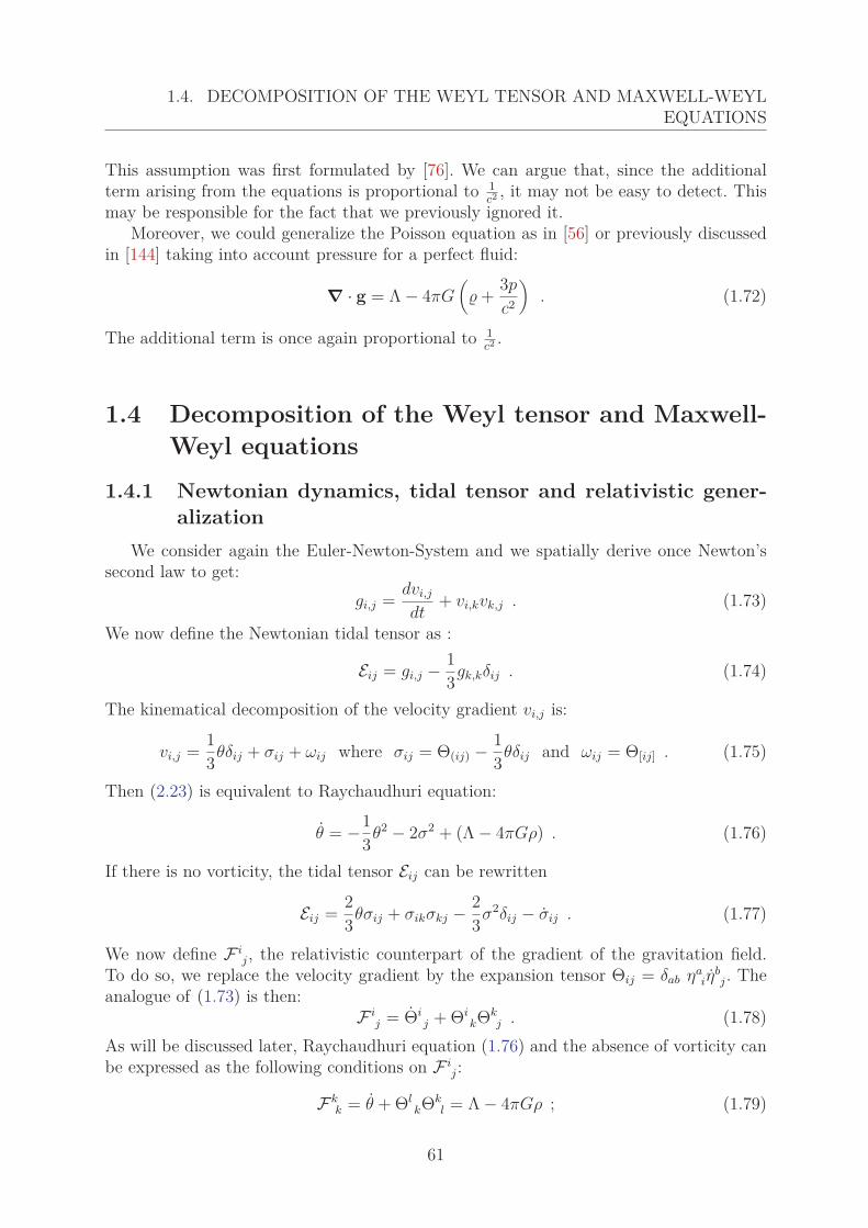
1.4. DECOMPOSITION OF THE WEYL TENSOR AND MAXWELL-WEYLEQUATIONS
This assumption was first formulated by [76]. We can argue that, since the additionalterm arising from the equations is proportional to 1
c2 , it may not be easy to detect. Thismay be responsible for the fact that we previously ignored it.
Moreover, we could generalize the Poisson equation as in [56] or previously discussedin [144] taking into account pressure for a perfect fluid:
∇ · g = Λ − 4πG(
+ 3p
c2
). (1.72)
The additional term is once again proportional to 1c2 .
1.4 Decomposition of the Weyl tensor and Maxwell-Weyl equations
1.4.1 Newtonian dynamics, tidal tensor and relativistic gener-alization
We consider again the Euler-Newton-System and we spatially derive once Newton’ssecond law to get:
gi,j = dvi,j
dt+ vi,kvk,j . (1.73)
We now define the Newtonian tidal tensor as :
Eij = gi,j − 13gk,kδij . (1.74)
The kinematical decomposition of the velocity gradient vi,j is:
vi,j = 13θδij + σij + ωij where σij = Θ(ij) − 1
3θδij and ωij = Θ[ij] . (1.75)
Then (2.23) is equivalent to Raychaudhuri equation:
θ = −13θ2 − 2σ2 + (Λ − 4πGρ) . (1.76)
If there is no vorticity, the tidal tensor Eij can be rewritten
Eij = 23θσij + σikσkj − 2
3σ2δij − σij . (1.77)
We now define F ij, the relativistic counterpart of the gradient of the gravitation field.
To do so, we replace the velocity gradient by the expansion tensor Θij = δab ηaiη
bj. The
analogue of (1.73) is then:F i
j = Θij + Θi
kΘkj . (1.78)
As will be discussed later, Raychaudhuri equation (1.76) and the absence of vorticity canbe expressed as the following conditions on F i
j:
Fkk = θ + Θl
kΘkl = Λ − 4πGρ ; (1.79)
61
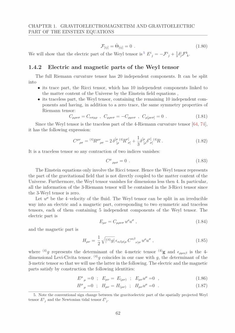
CHAPTER 1. GRAVITOELECTROMAGNETISM AND GRAVITOELECTRICPART OF THE EINSTEIN EQUATIONS
F[ij] = Θ[ij] = 0 . (1.80)We will show that the electric part of the Weyl tensor is 5 Ei
j = −F ij + 1
3δijFk
k.
1.4.2 Electric and magnetic parts of the Weyl tensorThe full Riemann curvature tensor has 20 independent components. It can be split
into• its trace part, the Ricci tensor, which has 10 independent components linked to
the matter content of the Universe by the Einstein field equations ,• its traceless part, the Weyl tensor, containing the remaining 10 independent com-
ponents and having, in addition to a zero trace, the same symmetry properties ofRiemann tensor:
Cμρνσ = Cνσμρ , Cμρνσ = −Cρμνσ , Cμ[ρνσ] = 0 . (1.81)Since the Weyl tensor is the traceless part of the 4-Riemann curvature tensor [64, 74],
it has the following expression:
Cμνρσ = (4)Rμν
ρσ − 2 δ[μ[ρ
(4)Rν]σ] + 1
3δ[μ[ρδ
ν]σ]
(4)R . (1.82)
It is a traceless tensor so any contraction of two indices vanishes:
Cμρμσ = 0 . (1.83)
The Einstein equations only involve the Ricci tensor. Hence the Weyl tensor representsthe part of the gravitational field that is not directly coupled to the matter content of theUniverse. Furthermore, the Weyl tensor vanishes for dimensions less then 4. In particular,all the information of the 3-Riemann tensor will be contained in the 3-Ricci tensor sincethe 3-Weyl tensor is zero.
Let uμ be the 4–velocity of the fluid. The Weyl tensor can be split in an irreducibleway into an electric and a magnetic part, corresponding to two symmetric and tracelesstensors, each of them containing 5 independent components of the Weyl tensor. Theelectric part is
Eμν = Cμρνσ uρuσ , (1.84)and the magnetic part is
Hμν = 12
√|(4)g| εαβρ(μ Cαβ
ν)σ uρuσ , (1.85)
where (4)g represents the determinant of the 4-metric tensor (4)g and ερμαβ is the 4-dimensional Levi-Civita tensor. (4)g coincides in our case with g, the determinant of the3-metric tensor so that we will use the latter in the following. The electric and the magneticparts satisfy by construction the following identities:
Eμμ =0 ; Eμν = E(μν) ; Eμνuμ =0 , (1.86)
Hμμ =0 ; Hμν = H(μν) ; Hμνuμ =0 . (1.87)
5. Note the conventional sign change between the gravitoelectric part of the spatially projected Weyltensor Ei
j and the Newtonian tidal tensor E ij .
62
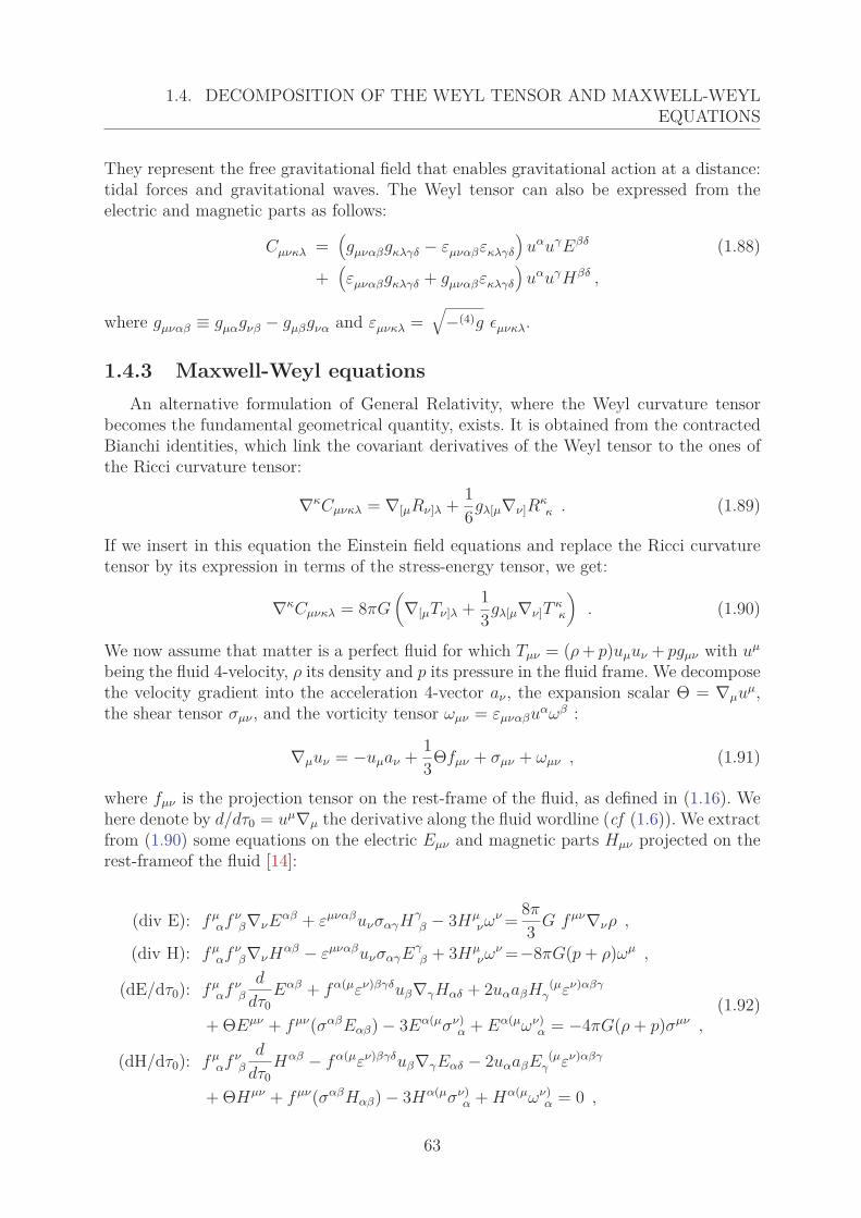
1.4. DECOMPOSITION OF THE WEYL TENSOR AND MAXWELL-WEYLEQUATIONS
They represent the free gravitational field that enables gravitational action at a distance:tidal forces and gravitational waves. The Weyl tensor can also be expressed from theelectric and magnetic parts as follows:
Cμνκλ =(gμναβgκλγδ − εμναβεκλγδ
)uαuγEβδ (1.88)
+(εμναβgκλγδ + gμναβεκλγδ
)uαuγHβδ ,
where gμναβ ≡ gμαgνβ − gμβgνα and εμνκλ =√
−(4)g εμνκλ.
1.4.3 Maxwell-Weyl equationsAn alternative formulation of General Relativity, where the Weyl curvature tensor
becomes the fundamental geometrical quantity, exists. It is obtained from the contractedBianchi identities, which link the covariant derivatives of the Weyl tensor to the ones ofthe Ricci curvature tensor:
∇κCμνκλ = ∇[μRν]λ + 16gλ[μ∇ν]R
κκ . (1.89)
If we insert in this equation the Einstein field equations and replace the Ricci curvaturetensor by its expression in terms of the stress-energy tensor, we get:
∇κCμνκλ = 8πG(
∇[μTν]λ + 13gλ[μ∇ν]T
κκ
). (1.90)
We now assume that matter is a perfect fluid for which Tμν = (ρ + p)uμuν + pgμν with uμ
being the fluid 4-velocity, ρ its density and p its pressure in the fluid frame. We decomposethe velocity gradient into the acceleration 4-vector aν , the expansion scalar Θ = ∇μuμ,the shear tensor σμν , and the vorticity tensor ωμν = εμναβuαωβ :
∇μuν = −uμaν + 13Θfμν + σμν + ωμν , (1.91)
where fμν is the projection tensor on the rest-frame of the fluid, as defined in (1.16). Wehere denote by d/dτ0 = uμ∇μ the derivative along the fluid wordline (cf (1.6)). We extractfrom (1.90) some equations on the electric Eμν and magnetic parts Hμν projected on therest-frameof the fluid [14]:
(div E): fμαf ν
β∇νEαβ + εμναβuνσαγHγβ − 3Hμ
νων = 8π
3 G fμν∇νρ ,
(div H): fμαf ν
β∇νHαβ − εμναβuνσαγEγβ + 3Hμ
νων =−8πG(p + ρ)ωμ ,
(dE/dτ0): fμαf ν
β
d
dτ0Eαβ + fα(μεν)βγδuβ∇γHαδ + 2uαaβH (μ
γ εν)αβγ
+ ΘEμν + fμν(σαβEαβ) − 3Eα(μσν)α + Eα(μων)
α = −4πG(ρ + p)σμν ,
(dH/dτ0): fμαf ν
β
d
dτ0Hαβ − fα(μεν)βγδuβ∇γEαδ − 2uαaβE (μ
γ εν)αβγ
+ ΘHμν + fμν(σαβHαβ) − 3Hα(μσν)α + Hα(μων)
α = 0 ,
(1.92)
63
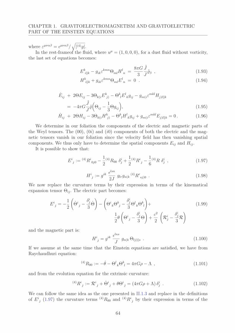
CHAPTER 1. GRAVITOELECTROMAGNETISM AND GRAVITOELECTRICPART OF THE EINSTEIN EQUATIONS
where εμναβ = εμναβ/√
|(4)g|.In the rest-frameof the fluid, where uμ = (1, 0, 0, 0), for a dust fluid without vorticity,
the last set of equations becomes:
Eki‖k − gikεkmnΘmlH
ln = 8πG
3J
J|i , (1.93)
Hki‖k + gikεkmnΘmlE
ln = 0 . (1.94)
Eij + 2ΘEij − 3Θk(iEkj) − Θk
lElkgij − gm(iε
mklHj)l‖k
= −4πGJ
J(
Θij − 13Θgij
), (1.95)
Hij + 2ΘHij − 3Θk(iHkj) − Θk
lHlkgij + gm(iε
mklEj)l‖k = 0 . (1.96)
We determine in our foliation the components of the electric and magnetic parts ofthe Weyl tensors. The (00), (0i) and (i0) components of both the electric and the mag-netic tensors vanish in our foliation since the velocity field has then vanishing spatialcomponents. We thus only have to determine the spatial components Eij and Hij.
It is possible to show that:
Eij := (4)Ri
0j0 − 12
(4)R00 δij + 1
2(4)Ri
j − 16
(4)R δij , (1.97)
H ij := gik εlsn
2Jglrgn(k
(4)Rrsj)0 . (1.98)
We now replace the curvature terms by their expression in terms of the kinematicalexpansion tensor Θij. The electric part becomes:
Eij = −1
2
(Θi
j −δi
j
3 Θ)
−(
ΘikΘk
j −δi
j
3 ΘlkΘk
l
)+ (1.99)
12θ
(Θi
j −δi
j
3 Θ)
+ c2
2
(Ri
j −δi
j
3 R)
and the magnetic part is:
H ij = gik εlns
Jgn(k Θlj)‖s . (1.100)
If we assume at the same time that the Einstein equations are satisfied, we have fromRaychaudhuri equation:
(4)R00 := −θ − ΘlkΘk
l = 4πGρ − Λ , (1.101)
and from the evolution equation for the extrinsic curvature:(4)Ri
j := Rij + Θi
j + θΘij = (4πGρ + Λ) δi
j . (1.102)
We can follow the same idea as the one presented in II.1.3 and replace in the definitionsof Ei
j (1.97) the curvature terms (4)R00 and (4)Rij by their expression in terms of the
64
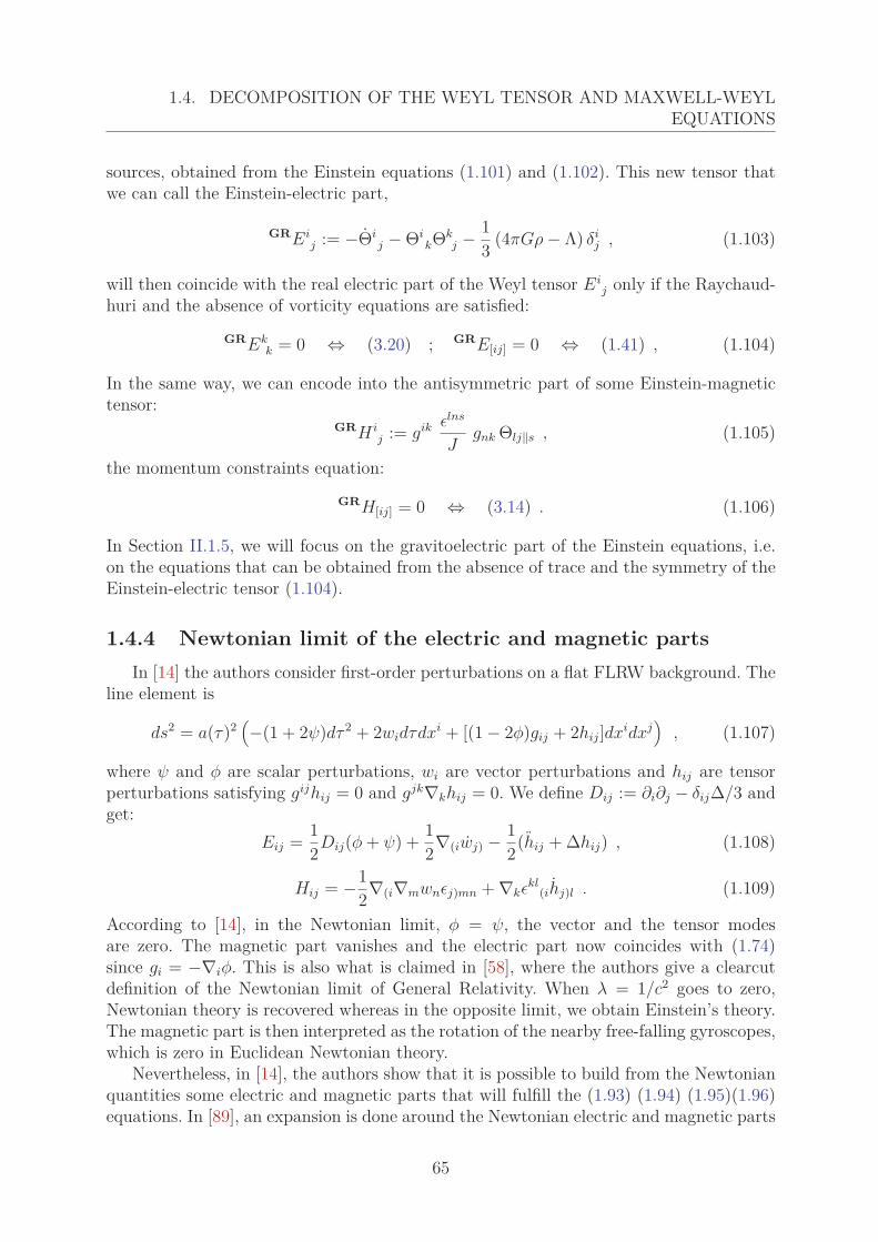
1.4. DECOMPOSITION OF THE WEYL TENSOR AND MAXWELL-WEYLEQUATIONS
sources, obtained from the Einstein equations (1.101) and (1.102). This new tensor thatwe can call the Einstein-electric part,
GREij := −Θi
j − ΘikΘk
j − 13 (4πGρ − Λ) δi
j , (1.103)
will then coincide with the real electric part of the Weyl tensor Eij only if the Raychaud-
huri and the absence of vorticity equations are satisfied:
GREkk = 0 ⇔ (3.20) ; GRE[ij] = 0 ⇔ (1.41) , (1.104)
In the same way, we can encode into the antisymmetric part of some Einstein-magnetictensor:
GRH ij := gik εlns
Jgnk Θlj‖s , (1.105)
the momentum constraints equation:
GRH[ij] = 0 ⇔ (3.14) . (1.106)
In Section II.1.5, we will focus on the gravitoelectric part of the Einstein equations, i.e.on the equations that can be obtained from the absence of trace and the symmetry of theEinstein-electric tensor (1.104).
1.4.4 Newtonian limit of the electric and magnetic partsIn [14] the authors consider first-order perturbations on a flat FLRW background. The
line element is
ds2 = a(τ)2(−(1 + 2ψ)dτ 2 + 2widτdxi + [(1 − 2φ)gij + 2hij]dxidxj
), (1.107)
where ψ and φ are scalar perturbations, wi are vector perturbations and hij are tensorperturbations satisfying gijhij = 0 and gjk∇khij = 0. We define Dij := ∂i∂j − δijΔ/3 andget:
Eij = 12Dij(φ + ψ) + 1
2∇(iwj) − 12(hij + Δhij) , (1.108)
Hij = −12∇(i∇mwnεj)mn + ∇kεkl
(ihj)l . (1.109)
According to [14], in the Newtonian limit, φ = ψ, the vector and the tensor modesare zero. The magnetic part vanishes and the electric part now coincides with (1.74)since gi = −∇iφ. This is also what is claimed in [58], where the authors give a clearcutdefinition of the Newtonian limit of General Relativity. When λ = 1/c2 goes to zero,Newtonian theory is recovered whereas in the opposite limit, we obtain Einstein’s theory.The magnetic part is then interpreted as the rotation of the nearby free-falling gyroscopes,which is zero in Euclidean Newtonian theory.
Nevertheless, in [14], the authors show that it is possible to build from the Newtonianquantities some electric and magnetic parts that will fulfill the (1.93) (1.94) (1.95)(1.96)equations. In [89], an expansion is done around the Newtonian electric and magnetic parts
65
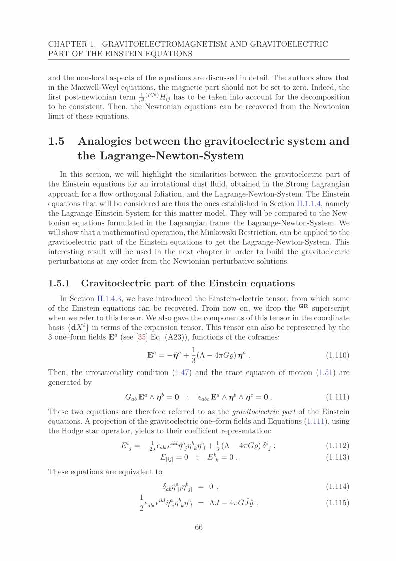
CHAPTER 1. GRAVITOELECTROMAGNETISM AND GRAVITOELECTRICPART OF THE EINSTEIN EQUATIONS
and the non-local aspects of the equations are discussed in detail. The authors show thatin the Maxwell-Weyl equations, the magnetic part should not be set to zero. Indeed, thefirst post-newtonian term 1
c3(P N)Hij has to be taken into account for the decomposition
to be consistent. Then, the Newtonian equations can be recovered from the Newtonianlimit of these equations.
1.5 Analogies between the gravitoelectric system andthe Lagrange-Newton-System
In this section, we will highlight the similarities between the gravitoelectric part ofthe Einstein equations for an irrotational dust fluid, obtained in the Strong Lagrangianapproach for a flow orthogonal foliation, and the Lagrange-Newton-System. The Einsteinequations that will be considered are thus the ones established in Section II.1.1.4, namelythe Lagrange-Einstein-System for this matter model. They will be compared to the New-tonian equations formulated in the Lagrangian frame: the Lagrange-Newton-System. Wewill show that a mathematical operation, the Minkowski Restriction, can be applied to thegravitoelectric part of the Einstein equations to get the Lagrange-Newton-System. Thisinteresting result will be used in the next chapter in order to build the gravitoelectricperturbations at any order from the Newtonian perturbative solutions.
1.5.1 Gravitoelectric part of the Einstein equationsIn Section II.1.4.3, we have introduced the Einstein-electric tensor, from which some
of the Einstein equations can be recovered. From now on, we drop the GR superscriptwhen we refer to this tensor. We also gave the components of this tensor in the coordinatebasis {dX i} in terms of the expansion tensor. This tensor can also be represented by the3 one–form fields Ea (see [35] Eq. (A23)), functions of the coframes:
Ea = −ηa + 13(Λ − 4πG) ηa . (1.110)
Then, the irrotationality condition (1.47) and the trace equation of motion (1.51) aregenerated by
Gab Ea ∧ ηb = 0 ; εabc Ea ∧ ηb ∧ ηc = 0 . (1.111)
These two equations are therefore referred to as the gravitoelectric part of the Einsteinequations. A projection of the gravitoelectric one–form fields and Equations (1.111), usingthe Hodge star operator, yields to their coefficient representation:
Eij = − 1
2Jεabcε
iklηajη
bkηc
l + 13 (Λ − 4πG) δi
j ; (1.112)E[ij] = 0 ; Ek
k = 0 . (1.113)
These equations are equivalent to
δabηa[iη
bj] = 0 , (1.114)
12εabcε
iklηaiη
bkηc
l = ΛJ − 4πGJ , (1.115)
66
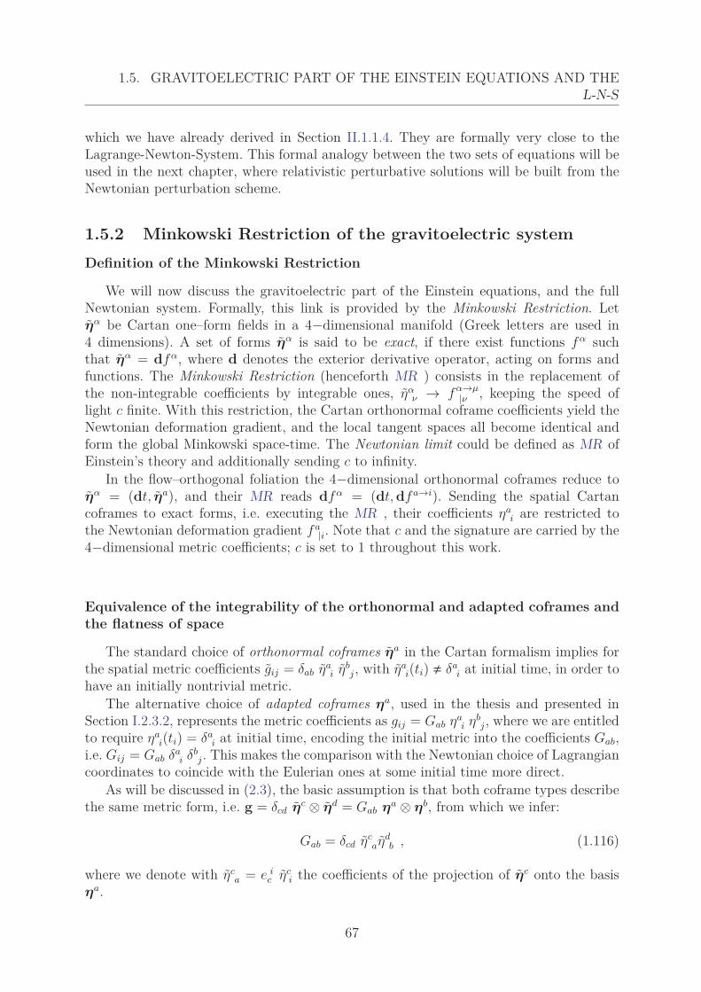
1.5. GRAVITOELECTRIC PART OF THE EINSTEIN EQUATIONS AND THEL-N-S
which we have already derived in Section II.1.1.4. They are formally very close to theLagrange-Newton-System. This formal analogy between the two sets of equations will beused in the next chapter, where relativistic perturbative solutions will be built from theNewtonian perturbation scheme.
1.5.2 Minkowski Restriction of the gravitoelectric system
Definition of the Minkowski Restriction
We will now discuss the gravitoelectric part of the Einstein equations, and the fullNewtonian system. Formally, this link is provided by the Minkowski Restriction. Letηα be Cartan one–form fields in a 4−dimensional manifold (Greek letters are used in4 dimensions). A set of forms ηα is said to be exact, if there exist functions fα suchthat ηα = dfα, where d denotes the exterior derivative operator, acting on forms andfunctions. The Minkowski Restriction (henceforth MR ) consists in the replacement ofthe non-integrable coefficients by integrable ones, ηα
ν → fα→μ|ν , keeping the speed of
light c finite. With this restriction, the Cartan orthonormal coframe coefficients yield theNewtonian deformation gradient, and the local tangent spaces all become identical andform the global Minkowski space-time. The Newtonian limit could be defined as MR ofEinstein’s theory and additionally sending c to infinity.
In the flow–orthogonal foliation the 4−dimensional orthonormal coframes reduce toηα = (dt, ηa), and their MR reads dfα = (dt, dfa→i). Sending the spatial Cartancoframes to exact forms, i.e. executing the MR , their coefficients ηa
i are restricted tothe Newtonian deformation gradient fa
|i. Note that c and the signature are carried by the4−dimensional metric coefficients; c is set to 1 throughout this work.
Equivalence of the integrability of the orthonormal and adapted coframes andthe flatness of space
The standard choice of orthonormal coframes ηa in the Cartan formalism implies forthe spatial metric coefficients gij = δab ηa
i ηbj, with ηa
i(ti) � δai at initial time, in order to
have an initially nontrivial metric.The alternative choice of adapted coframes ηa, used in the thesis and presented in
Section I.2.3.2, represents the metric coefficients as gij = Gab ηai ηb
j, where we are entitledto require ηa
i(ti) = δai at initial time, encoding the initial metric into the coefficients Gab,
i.e. Gij = Gab δai δb
j. This makes the comparison with the Newtonian choice of Lagrangiancoordinates to coincide with the Eulerian ones at some initial time more direct.
As will be discussed in (2.3), the basic assumption is that both coframe types describethe same metric form, i.e. g = δcd ηc ⊗ ηd = Gab ηa ⊗ ηb, from which we infer:
Gab = δcd ηcaηd
b , (1.116)
where we denote with ηca = e i
c ηci the coefficients of the projection of ηc onto the basis
ηa.
67
CHAPTER 1. GRAVITOELECTROMAGNETISM AND GRAVITOELECTRICPART OF THE EINSTEIN EQUATIONS
The MR applied to either of these coframes requires them to be exact forms, ηa = dfa
or ηa = dfa. They then define some global Eulerian coordinates, xa and xa, respectively.In the MR , Eq. (1.116) is equivalent to
Gab = δcd∂f c
∂xa
∂fd
∂xb. (1.117)
We infer from (1.117) that the coefficients Gab just depend on initial vector displacementsafter executing the MR . They are related to the initial deformation gradient in theorthonormal description, as can be seen by looking at the metric equivalence relation inan exact Lagrangian basis, g = gij dX i ⊗ dXj = gij dX i ⊗ dXj:
g(Xk, ti) = δabfa|Xi(Xk, ti)f b
|Xj (Xk, ti)dX i ⊗ dXj
= δabfa|i(Xk, ti)f b
|j(Xk, ti)dX i ⊗ dXj
= Gab(Xk)δaiδ
bjdX i ⊗ dXj , (1.118)
where a slash denotes derivative with respect to the coordinates X i, as in the main text,and it is explicitly noted otherwise. From (1.117) we conclude that
g = Gab ηa ⊗ ηb = δcd∂f c
∂xa
∂fd
∂xbdxa ⊗ dxb = δcd dxc ⊗ dxd , (1.119)
which is the Euclidean metric.Summarizing: execution of the MR leads, in either of the chosen coframes, to a metric
that is equivalent to the Euclidean metric. The coefficients Gab can then be expressed interms of initial vector displacements, cf. Eq. (1.118).
Minkowski Restriction of the gravitoelectric part of the Einstein equations
In the MR , (1.114) becomes
δabfa|[i f b
|j] = 0 , (1.120)
i.e. is equal to (2.48). Since, for a flat space-time J = 1, (1.115) becomes
12εabcε
iklfa|i f b
|k f c|l = ΛJ − 4πG (1.121)
i.e. is equal to (2.47). So, the gravitoelectric part of the Einstein equations (1.114) (1.115)then reduces to the Lagrange-Newton-System. Moreover, we obtained the Lagrange-Newton-System expressed in the inertial frame, i.e. for f = g. Therefore, f is then solutionof the following equations:
∇ × f = 0 , (1.122)∇ · f = Λ − 4πG . (1.123)
(1.122) implies that f = −∇φ, where φ is a scalar potential solution of the Poissonequation.
68
1.5. GRAVITOELECTRIC PART OF THE EINSTEIN EQUATIONS AND THEL-N-S
The MR operation closes the system, reducing the number of free functions from nine(ηa
i(Xk, t)) to three (f i(Xk, t)). A discussion of the MR for the remaining equations,yielding nontrivial Newtonian analogs, will be done in Section II.1.5.3. Considering onlythe gravitoelectric equations is not enough to determine the nine functions of the coframecoefficients. The relativistic aspects contained in the remaining equations will lead to aricher structure of the solutions and also to constraints on solutions of the gravitoelectricsystem. A follow–up work will explicitly consider both parts in the framework of first–order solutions. To conclude, the Lagrange–Einstein gravitoelectric equations are (up tonon-integrability) equivalent to their Newtonian analogue but the remaining equations donot have an obvious Newtonian counterpart.
1.5.3 Minkowski Restriction of the other Einstein equationsThe equations that we left to be interpreted are the momentum constraints, the one
containing the Ricci scalar (1.125) and the one containing the traceless part of the Riccitensor (1.127) τ i
j, obtained from the traceless part of the evolution equation for theextrinsic curvature (1.42):(
εabcεiklηa
jηbkηc
l
)‖i
=(εabcε
iklηaiη
bkηc
l
)‖j
, (1.124)
εabcεmklηa
mηbkηc
l = 16πGJ + 2ΛJ − c2 JR , (1.125)12
(εabcε
iklηajη
bkηc
l − 13εabcε
mklηamηb
kηclδ
ij
)(1.126)
+(
εabcεiklηa
j ηbkηc
l − 13εabcε
mklηamηb
kηclδ
ij
)=−c2 Jτ i
j .
Considering a flat space-time in the frame of General Relativity would automaticallylead to a zero curvature Ri
j = 0. Here, we no longer work in the frame of GeneralRelativity since we decouple the geometry of space-time and the dynamics of the fluid.In this context, Ri
j is no longer a geometrical term but should be reinterpreted.To have an intuition of the new meaning of Ri
j, we first consider the Newtonian case fora homogeneous isotropic universe. Newton’s second law combined with Poisson equationleads to (1.9). Integrating it gives the equation (1.9) that we remind here:
(a
a
)2− 8πG
3 ρH − Λ3 + k
a2 = 0 , (1.127)
By identifying this equation, called Friedmann’s equation, to Hamiltonian constraint fora Universe with constant curvature NR, we can show that:
k
a2 = c2NR6 . (1.128)
We have shown that the equations (1.125) and (1.127), contain, in the frame of GeneralRelativity, some information that has no Newtonian counterpart. Here, these supplemen-tary equations should not be interpreted as equalities but rather as some kinematicaldefinitions for the Minkowskian analogue of curvature: MRi
j. The following equations aregeneral but their interpretation is specific to our approach.
69
CHAPTER 1. GRAVITOELECTROMAGNETISM AND GRAVITOELECTRICPART OF THE EINSTEIN EQUATIONS
The Raychaudhuri equation (1.115) can be rewritten:
θ + 13θ2 + 2σ2 + 4πGρ − Λ = 0 . (1.129)
If we define l = J1/3, it becomes:
3 l
l+ 2σ2 + 4πGρ − Λ = 0 . (1.130)
This equation is equivalent to:
σ2 + 2θσ2 = 12
MR + 13
MR θ , (1.131)
which can be rewritten as:
6(σ2 MR)1/2 (J [σ2]1/2)˙ = (J MR3/2)˙ . (1.132)
Since the integral of (1.130) has to be the Hamiltonian constraint, a ‘Minkowskian curva-ture’ term can be defined form integration constants and kinematical quantities:
MR := 2σ2 − 8l2
∫σ2l ldt − 2
(σ2 − 12
MR)l2 . (1.133)
Finally, we obtained an evolution equation for MR as a function of the shear. We cancheck that, in the case of a homogeneous isotropic flow, we recover the Newtonian result(1.128) since then l(t) = a(t). From (1.127) and Hamiltonian constraint we can defineMRi
j from kinematical quantities (shear and expansion) and integration constants 6:
MRij := 2
3δij [σ2 − 1
3θ2 + 8πGρ + Λ] − σij − θ σi
j , (1.134)
MRij := 1
3δij
MR − σij − θ σi
j . (1.135)
1.6 Concluding remarksIn this chapter we presented various ways to approach the GEM analogy. We first con-
sidered the similarities between the Newtonian theory of gravity and electrodynamics. Wethen built a generalization of the field equations for the gravitational field and for New-ton’s second law. We have then shown that the Euler-Newton-System could be obtainedin the limit where the speed c goes to infinity. Afterwards, we turned to General Relativityand developed the GEM approach based on the decomposition of the Weyl tensor into anelectric and a magnetic part. As was discussed, these fields satisfy equations that exhibitsimilarities with the Maxwell equations. Nevertheless, contrary to electrodynamics, theelectric and the magnetic parts of the Weyl tensor do not play similar roles. The electric
6. Setting MRij to zero would have led to a conservation equation for σi
j which would have restrictedthe problem to a self similar flow.
70
1.6. CONCLUDING REMARKS
part is the relativistic generalization of the Newtonian tidal tensor whereas the magneticpart encodes the dynamics of gravitational waves. A Newtonian limit of the electric andmagnetic parts has also been discussed in order to better understand what they containin the relativistic case.
In this chapter, we also discussed the analogies between the gravitoelectric part ofthe Einstein equations and the Lagrange-Newton-System. The Minkowski Restriction,which is the mathematical operation that enables us to go from the gravitoelectric partof the Einstein equations to the Lagrange-Newton-System, was also applied to the otherEinstein equations. Nevertheless, since the Minkowski Restriction decouples the geometryof space-time from the dynamics of the fluid (the geometrical Ricci curvature tensor beingthen zero), an alternative interpretation of the curvature terms in terms of the kinematicalproperties of the fluid has then been formulated.
71
Chapter 2
Gravitoelectric Perturbation andSolution Schemes at Any Order
This chapter is based on the paper by A. Alles, T. Buchert, F. Al Roumi andA. Wiegand [4].
Contents2.1 Construction schemes for relativistic perturbations and so-
lutions . . . . . . . . . . . . . . . . . . . . . . . . . . . . . . . . . 752.1.1 General n–th order perturbation scheme . . . . . . . . . . . . . 752.1.2 Initial data for the perturbation scheme . . . . . . . . . . . . . 76
General initial data setting for the perturbations . . . . . . . . 76Relativistic counterpart of the Poisson equation and consequences
for Wa . . . . . . . . . . . . . . . . . . . . . . . . . . 77Summary of initial data . . . . . . . . . . . . . . . . . . . . . . 78
2.1.3 Gravitoelectric perturbation scheme . . . . . . . . . . . . . . . 79Recap: Newtonian theory . . . . . . . . . . . . . . . . . . . . . 79Einstein’s theory . . . . . . . . . . . . . . . . . . . . . . . . . . 82
2.1.4 Gravitoelectric solution scheme . . . . . . . . . . . . . . . . . . 83Recap: Newtonian theory . . . . . . . . . . . . . . . . . . . . . 83Einstein’s Theory . . . . . . . . . . . . . . . . . . . . . . . . . . 83
2.2 Application of the solution scheme . . . . . . . . . . . . . . . . 842.2.1 Systematics of the solutions . . . . . . . . . . . . . . . . . . . . 842.2.2 Reconstruction of the relativistic solutions . . . . . . . . . . . . 85
Trace part . . . . . . . . . . . . . . . . . . . . . . . . . . . . . . 85Antisymmetric part . . . . . . . . . . . . . . . . . . . . . . . . 85Tracefree symmetric part . . . . . . . . . . . . . . . . . . . . . 86
2.2.3 Example 1: recovering parts of the general first–order solution . 862.2.4 Example 2: constructing second–order solutions for ‘slaved ini-
tial data’ . . . . . . . . . . . . . . . . . . . . . . . . . . . . . . 892.3 Summary and concluding remarks . . . . . . . . . . . . . . . . 91
72
In Section II.1.1.3, we presented the Einstein’s equations in the 3 + 1 form for theCartan coframe variable. In previous work, the first–order solution was investigated forthe trace and antisymmetric parts. The solution then obtained was extrapolated in thespirit of Zel’dovich’s approximation in Newtonian cosmology. Moreover, a definition ofa nonperturbative scheme of structure formation [35] was also provided. The averageproperties of the latter in relation to the Dark Energy and Dark Matter problems werestudied by T. Buchert, C. Nayet and A. Wiegand in [36]. Here, we proceed by providingthe gravitoelectric subclass of relativistic nth–order perturbation and solution schemes.As in previous work we restrict our attention to irrotational dust continua for simplicity.
The problem of perturbation solutions in general relativity has been addressed by manyworks. In cosmology the ‘standard approach’ is based on the gauge invariant ‘Bardeen for-malism’ (for a selection of key references on standard perturbation theory see Refs. [10],[112], [88], [51]). A covariant and gauge–invariant approach has been proposed [62, 63].The reason for the existence of various approaches is due to an ambiguity of the choiceof perturbation variable, the choice of a ‘background’, but also due to different philoso-phies; e.g. the standard gauge–invariant approach compares the physical manifold with areference ‘background manifold’, while others solely operate on the physical manifold.
The conceptual difference of our framework lies in the fact that we no longer considera reference background manifold. All the quantities are now defined on the physical spacesection. All orders of the perturbations are defined on the physical manifold, not withrespect to a zero–order manifold (that was interpreted as the background manifold instandard perturbation theory). Moreover, we are perturbing a single dynamical variable,the Cartan coframes. As a consequence, the issue of gauge invariance does not arise;covariance or diffeomorphism invariance is guaranteed for a given foliation of spacetimeby using Cartan differential forms.
A similar point of view has also been taken in previous work, i.e. the pioneering workby Kasai presents a relativistic generalization of the ‘Zel’dovich approximation’ [161],and followup works with his collaborators present a class of second–order perturbationsolutions [85, 131]; see also the earlier papers by Tomita [146, 147, 148], the paper bySalopek et al. [132] as well as the series of papers by Matarrese, Pantano and Saez [105,106, 107], considerations of so–called ‘silent universe models’ [11, 89, 14, 19, 66], and therecent paper [122]. These works are all in a wider sense concerned with the relativisticLagrangian perturbation theory and concentrate on an intrinsic, covariant description ofperturbations. Still, the present work takes another angle and goes beyond some conceptsof these latter works, as we now explain. In this work, we consider, as presented in SectionII.1.1.4, the Einstein equations formulated within a flow–orthogonal foliation with a singledynamical variable: the spatial Cartan coframe fields. As we have seen in Section II.1.5,they generalize the Lagrangian deformation gradient being the single dynamical variablein the Newtonian theory. One advantage of this approach is that only perturbations ofthis variable are considered, which entitles us to express all other physical quantities asfunctionals of this variable. Thus, it is possible to leave the strictly perturbative frameworkand to construct nonperturbative models inserting the deformation solutions at a givenorder of expansion of the Einstein equations into the functional definitions of these fields,without a posteriori expanding the functional expressions. This in turn provides highlynonlinear approximations for structure formation (e.g., the density field is known through
73
an exact integral of the perturbation variable; the metric as a bilinear form maintains itsrole as a measure of distance, i.e. as a quadratic expression; the curvatures are the generaldefining functionals for the given perturbed space, etc.).
Moreover, we provide construction rules to derive relativistic perturbative solutionsfrom the known Newtonian solutions at any order of the perturbations: we have to addi-tionally study the traceless symmetric part of the equations having no obvious Newtoniananalog, and which is fundamentally linked to the traceless Ricci tensor and the physics ofgravitational waves. Then, we give the perturbation and solution schemes to any orderof the perturbations for the gravitoelectric part of the Lagrange–Einstein system. Theseschemes cover the full Newtonian hierarchy of the Lagrangian perturbation theory usinga restriction rule that we will define. Thus, the results of this work allow us to constructthe relativistic counterpart of all Newtonian results, where higher–order information isneeded, e.g., to construct the bispectrum of the perturbations (cf. Refs. [120, 121]).
We perform a strictly intrinsic derivation, i.e., without reference to an external back-ground space. The perturbations are described locally (in coordinates of the tangentspaces at the physical manifold at each order of the perturbations). There is no need fora diffeomorphism to a global background manifold. Furthermore, the existence of such aglobal diffeomorphism depends on the global topology of the physical manifold which, ingeneral, needs several coordinate charts to cover it.
Einstein’s equations within a flow–orthogonal foliation of spacetime can be formulatedin terms of equations for the gravitoelectric and gravitomagnetic parts of the spatiallyprojected Weyl tensor, as we have shown in Section II.1.4. Subjecting the gravitoelectricsubsystem of equations to a MR , i.e. by sending the Cartan coframes to exact forms,we obtain the Newtonian system in Lagrangian form (cf Section II.1.5 and [35] ). Inthis chapter, we investigate the reverse process, i.e. the transposition from integrable tononintegrable deformations, which enables us to construct a gravitoelectric subclass ofthe relativistic perturbation and solution schemes that corresponds to the Newtonianperturbation and solution schemes.
While the Newtonian system furnishes a vector theory, where the gravitational fieldstrength is determined by its divergence and its curl (the trace and antisymmetric partsof the Eulerian field strength gradient), the so generalized schemes deliver nontrivialsolutions for the trace–free symmetric part that is connected to the gravitoelectric partof the spatially projected Weyl tensor, the Newtonian counterpart of which is the tidalfield tensor.
This section is structured as follows. In Section II.2.1 we investigate perturbationand solution schemes at any order n of the perturbations by explicitly paraphrasing theNewtonian schemes. Section II.2.2 explains the reconstruction rules and provides explicitexamples. Finally, Section II.2.3 sums up and discusses perspectives.
2.1. CONSTRUCTION SCHEMES FOR RELATIVISTIC PERTURBATIONS ANDSOLUTIONS
2.1 Construction schemes for relativistic perturba-tions and solutions at any order
We now turn to the main part of this part and construct the gravitoelectric subclassof nth–order relativistic perturbation and solution schemes through generalization of theknown Newtonian schemes. This allows furnishing relativistic inhomogeneous models forlarge–scale structure formation in the Universe. The successful Lagrangian perturbationtheory in Newtonian cosmology is well–developed. We will here generalize the perturbationand solution schemes of Newtonian cosmology given in the review [55], whose essentialsteps will be recalled in this section, followed by their relativistic counterparts.
All schemes are applied to the matter model ‘irrotational dust’. It is possible to extendthe present schemes by employing the framework for more general fluids in a Lagrangiandescription that will be developed in forthcoming work. Most of the known representationsare focused on writing equations in terms of tensor or form coefficients. Our investigationwill be guided by the compact differential forms formalism as before. However, we willalso project to the coefficient form in parallel to ease reading.
2.1.1 General n–th order perturbation schemeAs in standard perturbation theories, we decompose the perturbed quantity into a
Friedmann–Lemaître–Robertson–Walker (FLRW) solution and deviations thereof, whichare expanded up to a chosen order n of the perturbations. Contrary to the standardperturbation theory, we do not perturb the metric globally at the background space, butwe perturb the Cartan coframes locally:
ηa = ηaidX i = a(t)
(δa
i +∑
n
P a(n)i
)dX i , (2.1)
in the local exact basis dX i. Notice that with this ansatz we choose to perturb a zero–curvature FLRW model, but it is possible to encode an initial first–order constant curva-ture in the coefficient functions Gab in the following local metric coefficients, which canbe calculated from the above coframe ansatz:
gij = Gabηaiη
bj . (2.2)
We remind that, in order to obtain equations that are formally closer to the Newtonianones, we do not choose orthonormal (Cartan) coframes ηa as is common in the literature,but the ones called adapted coframes ηa. Furthermore, we can link these results to theones obtained for the orthonormal coframes ηc (compare also corresponding remarks in[40] and [74]). Indeed, the metric bilinear form can be written as:
g = δcd ηc ⊗ ηd = Gab ηa ⊗ ηb . (2.3)
From this identity, we conclude:
Gab = δcd ηcaηd
b , (2.4)
75
CHAPTER 2. GRAVITOELECTRIC PERTURBATION AND SOLUTIONSCHEMES AT ANY ORDER
where the ηca are the coefficients of the projection of ηc onto the basis ηa. In the next
subsection, we will specify the coframes we consider in such a way that the initial coframeperturbations vanish. From now on, we will call these coframes adapted coframes todistinguish them from the orthonormal ones.
2.1.2 Initial data for the perturbation schemeWe choose initial data in formal correspondence with the Lagrangian theory in Newto-
nian cosmology and generalize these initial fields to the relativistic stage. This has obviousadvantages with regard to the aim to give construction rules that translate the knownNewtonian solutions to general relativity. For the initial data setting in the Newtoniancase see [55].
General initial data setting for the perturbations
Let the three one–form fields Ua = UaidX i be the initial one–form generalization
of the Newtonian peculiar velocity–gradient, obtained by the inverse MR . Accordingly,let Wa = W a
idX i be the initial one–form generalization of the Newtonian peculiar–acceleration gradient. Our solutions will be written in terms of these initial data. Wesummarize them together with the constraints at the end of this paragraph.
By generalizing the Newtonian initial data, the initial data for the comoving per-turbation form coefficients read (we denote P a
i(ti) =: Pai, and correspondingly for its
time–derivatives):
Pai = 0 , (2.5)
Pai = Ua
i , (2.6)Pa
i = W ai − 2HiU
ai . (2.7)
We assume, without loss of generality [55], that the initial data are first–order. As shownin Paragraph II.2.1.2, the initial density contrast δi := (i −Hi)/Hi satisfies the equality:
δi(1) = δi = Hiδi = − 1
4πGδk
aW ak . (2.8)
Equation (2.5) implies that the coframes we will work with from now on are initiallyequal to the exact Lagrangian coordinate basis: ηa(ti) = δa
i dX i. This in turn providesthe initial metric coefficients in the form:
Gij = gij(ti) = Gabδaiδ
bj . (2.9)
In view of the flow–orthogonal foliation, we have the irrotationality constraint:
ω = Gabηa ∧ ηb = 0 =⇒ GabUa ∧ δb
jdXj = 0 . (2.10)
This implies for the coefficient functions: U[ij] = 0. (We used the implicit definitionUij := δb
iGbaUaj.)
76
2.1. CONSTRUCTION SCHEMES FOR RELATIVISTIC PERTURBATIONS ANDSOLUTIONS
Remark:From (2.4) and (2.5), it is interesting to notice the following relations that hold to zerothand first order (the full initial data are considered to be first order, as was also the choicein the Newtonian schemes [55]): ⎧⎪⎪⎨
⎪⎪⎩G(0)
ij = δij ;G(1)
ij = 2Pij ;2P(ij) = G(1)
ij + 2P(ij) ;(2.11)
where Pij = Pij(ti). We are thus able to rederive some results from the ones obtained inprevious works that used orthonormal coframes. For example, the Ricci curvature tensorat first–order can be obtained by inserting the identities (2.11) into (93) of [35]. We canso obtain the adapted coframes from the orthonormal ones and vice–versa.
Relativistic counterpart of the Poisson equation and consequences for Wa
In the Newtonian approach the initial peculiar–acceleration and the density inhomo-geneities are linked through the Poisson equation. In order to generalize this equationto the relativistic case, we note the following relativistic generalization of the Newtonianfield strength gradient that follows from inspection of the Lagrange–Einstein system (fordetails the reader can always consult [35]):
F ij := Θi
j + ΘikΘk
j (2.12)= −Ri
j − ΘΘij + (4πG − Λ) δi
j + ΘikΘk
j , (2.13)
with the 3−Ricci tensor coefficients Rij whose trace is the Ricci scalar R, and Θij theexpansion tensor coefficients. According to the energy constraint, R + Θ2 − Θk
�Θ�k =
6πG+2Λ, the symmetry of the expansion tensor and Ricci curvature, it is straightforwardto show that the relativistic gravitational field coefficients Fij respect the following fieldequations:
Fkk = Λ − 4πG ; F[ij] = 0 . (2.14)
In terms of the coframe fields, the relativistic gravitational field can be written as follows:
F ij = 1
2Jεabcε
iklηajη
bkηc
� . (2.15)
Hence, inserting the coframe perturbations and evaluating this expression at initialtime, we get the following relations (note that the zero–order fields trivially satisfy thesecond constraint):
Fkk(ti) = Λ − 4πGi = (2.16)
Λ − 4πGHi(1 + δi) = 3ai + δkaW a
k ; (2.17)F[ij](ti) = δb
[iGbaW aj] = W[ij] = 0 . , (2.18)
with the initial density contrast δi. Thus, the deviation one–form fields Wa obey thefollowing equations that generalize the Poisson equation for the inhomogeneous deviationsoff the zero–order solution:
∗12εabcWa ∧ δb
jdXj ∧ δckdXk = −4πGδi ; GabWa ∧ δb
jdXj = 0 ,
77
CHAPTER 2. GRAVITOELECTRIC PERTURBATION AND SOLUTIONSCHEMES AT ANY ORDER
with δi = i − Hi, implying for the coefficient functions:
− 14πG
δkaW a
k = δi = Hiδi ; W[ij] = 0 . (2.19)
Summary of initial data
We summarize the set of initial data, determined by our choice of the basis and sub-jected to the constraints. We assume in perturbative expansions, without loss of generality[55], that the initial data {(2.20) − (2.22)} are first order. We drop the index (1) for nota-tional ease and denote the initial data for the comoving perturbation form coefficients byP a
i(ti) =: Pai. We set:
— for the initial deformation and the initial generalizations of the Newtonian velocityand acceleration gradients:⎧⎪⎪⎨
⎪⎪⎩Pa(n) = 0 ∀n ,
Ua(1) = Ua, U[ij] = 0 ;Wa(1) = Wa, W[ij] = 0 ,
(2.20)
— where the coefficients are related via the initial values of the time–derivatives ofthe deformation: ⎧⎨
⎩Pai = Ua
i ;Pa
i = W ai − 2HiU
ai ,
(2.21)
— together with additional initial constraints that are to be respected (a relation tothe initial metric, to the initial density contrast, and the four ADM constraintequations evaluated at initial time):⎧⎪⎪⎪⎪⎪⎪⎨
⎪⎪⎪⎪⎪⎪⎩
Gij = Gab ηai(ti)ηb
j(ti) = Gabδaiδ
bj ;
4πGδi(1) = −W ;
HiU = −R(ti)4 − W ;(
Uajδ
ia
)||i = (Ua
iδi
a )|j ;
(2.22)
Here and in the following we use the abbreviations δkaUa
k =: U , δkaW a
k =: W forthe trace expressions.
— the initial Ricci curvature as found from the equation of motion (1.42):
Rij(ti) = −(W i
j + HiUij) − δi
j(W + HiU)−εabcε
ilkUajU
blδ
ck ; (2.23)
— equating this expression with the initial Ricci tensor as calculated from the initialmetric,
Rij(ti) = G i(1)
[j|b]Gb|a(1)a + G
b|a(1)j G i(1)
[b|a] + G a(1)b|j G [b|i](1)
a + 12 G a(1)
[a|b]Gb|i(1)j − 1
2G a|b(1)a G i(1)
[j|b]
+ 12G(1) a
b|[j G(1) b|ia] + 2G
(1) [a|i][j|a] + 2G
(2) [a|i][j|a] − 2G(1) a
b G[b|i](1)[j|a] − 2G(1) i
a G[b|a](1)[j|b] , (2.24)
78
2.1. CONSTRUCTION SCHEMES FOR RELATIVISTIC PERTURBATIONS ANDSOLUTIONS
we determine the first–order part of the initial metric (which is a derived quantity),
2G(1) [i|k][k|j] = −HiU
ij − W i
j − (HiU + W ) δij , (2.25)
— as well as the second–order part of the initial metric (which later appears in theperturbation and solution schemes):
2G(2) [i|k][k|j] = f(U i
j, W ij) , (2.26)
where the function f can again be derived by equating (2.24) and (2.13). All further ordersvanish.
The initial data given in (2.20) are exhaustive: in our ADM split, the system of equa-tions {(1.41) − (1.44)} contains 9 second–order equations of motion for the coframessubjected to 4 constraints. A general solution therefore contains 18 coefficient functionsencoded in Uij and Wij that reduce to 12 functions for solutions of the irrotationalityconditions (1.41), which these latter are represented by the 6 constraints U[ij] = 0 andW[ij] = 0. The general solution is further subjected to the 4 ADM constraints resulting incorresponding constraints on Uij and Wij.
2.1.3 Gravitoelectric perturbation schemeWe now recall the general Lagrangian perturbation scheme of Newtonian cosmology
and generalize it to a gravitoelectric scheme in relativistic cosmology. By construction,this latter will already contain the known Lagrangian perturbation scheme at any orderin the geometrical limit of exact deformation one–forms.
Recap: Newtonian theory
The general perturbation scheme has been fully developed in [55]. Our approach onlyslightly differs in terms of the initial conditions: we formulate them such that they areformally closer to the relativistic approach. Following the general ansatz (2.1), we intro-duce three comoving perturbation forms dP i of the three components of the comovingvector perturbation fields P i(X i, t):
df i( �X, t) =: a(t)dF i( �X, t) = a(t)(dX i + dP i( �X, t)
), (2.27)
and decompose the perturbation gradient field on the FLRW background order by order:
dP i =∞∑
m=1εmdP i(m) . (2.28)
It is, of course, possible to consider perturbations of the position fields f i, because theNewtonian equation can be expressed in a vectorial form. The relativistic equations are,however, tensorial and we, therefore, consider the representation in terms of the gradientof the fluid’s deformation.
In order to provide unique solutions of the Newtonian system, suitable boundaryconditions have to be imposed. For the cosmological framework the requirement of periodic
79
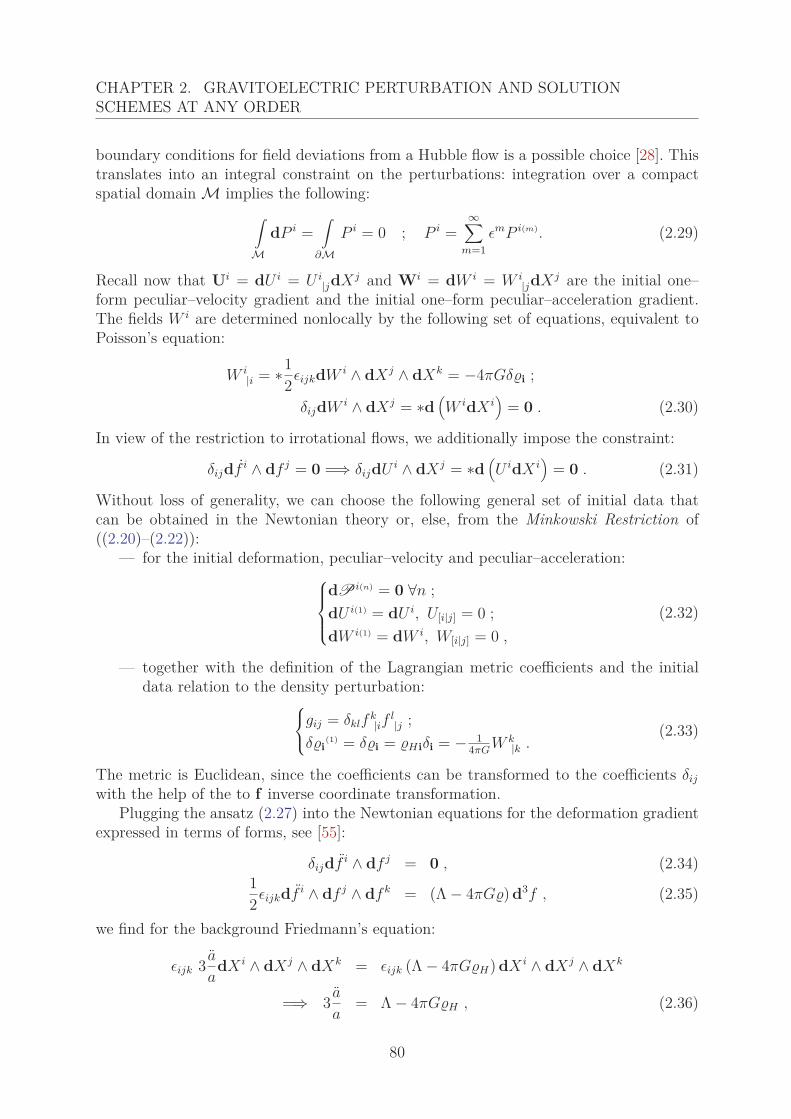
CHAPTER 2. GRAVITOELECTRIC PERTURBATION AND SOLUTIONSCHEMES AT ANY ORDER
boundary conditions for field deviations from a Hubble flow is a possible choice [28]. Thistranslates into an integral constraint on the perturbations: integration over a compactspatial domain M implies the following:
∫M
dP i =∫
∂MP i = 0 ; P i =
∞∑m=1
εmP i(m). (2.29)
Recall now that Ui = dU i = U i|jdXj and Wi = dW i = W i
|jdXj are the initial one–form peculiar–velocity gradient and the initial one–form peculiar–acceleration gradient.The fields W i are determined nonlocally by the following set of equations, equivalent toPoisson’s equation:
W i|i = ∗1
2εijkdW i ∧ dXj ∧ dXk = −4πGδi ;
δijdW i ∧ dXj = ∗d(W idX i
)= 0 . (2.30)
In view of the restriction to irrotational flows, we additionally impose the constraint:
δijdf i ∧ df j = 0 =⇒ δijdU i ∧ dXj = ∗d(U idX i
)= 0 . (2.31)
Without loss of generality, we can choose the following general set of initial data thatcan be obtained in the Newtonian theory or, else, from the Minkowski Restriction of((2.20)–(2.22)):
— for the initial deformation, peculiar–velocity and peculiar–acceleration:⎧⎪⎪⎨⎪⎪⎩
dP i(n) = 0 ∀n ;dU i(1) = dU i, U[i|j] = 0 ;dW i(1) = dW i, W[i|j] = 0 ,
(2.32)
— together with the definition of the Lagrangian metric coefficients and the initialdata relation to the density perturbation:⎧⎨
⎩gij = δklfk|if
l|j ;
δi(1) = δi = Hiδi = − 1
4πGW k
|k .(2.33)
The metric is Euclidean, since the coefficients can be transformed to the coefficients δij
with the help of the to f inverse coordinate transformation.Plugging the ansatz (2.27) into the Newtonian equations for the deformation gradient
expressed in terms of forms, see [55]:
δijdf i ∧ df j = 0 , (2.34)12εijkdf i ∧ df j ∧ dfk = (Λ − 4πG) d3f , (2.35)
we find for the background Friedmann’s equation:
εijk 3 a
adX i ∧ dXj ∧ dXk = εijk (Λ − 4πGH) dX i ∧ dXj ∧ dXk
=⇒ 3 a
a= Λ − 4πGH , (2.36)
80
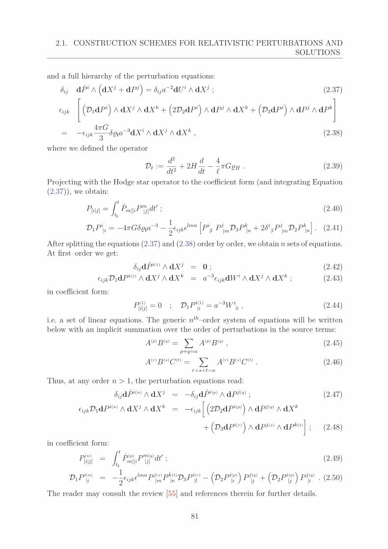
2.1. CONSTRUCTION SCHEMES FOR RELATIVISTIC PERTURBATIONS ANDSOLUTIONS
and a full hierarchy of the perturbation equations:δij dP i ∧
(dXj + dP j
)= δija
−2dU i ∧ dXj ; (2.37)
εijk
⎡⎣ (D1dP i
)∧ dXj ∧ dXk +
(2D2dP i
)∧ dP j ∧ dXk +
(D3dP i
)∧ dP j ∧ dP k
⎤⎦
= −εijk4πG
3 δia−3dX i ∧ dXj ∧ dXk , (2.38)
where we defined the operator
D� := d2
dt2 + 2Hd
dt− 4
�πGH . (2.39)
Projecting with the Hodge star operator to the coefficient form (and integrating Equation(2.37)), we obtain:
P[i|j] =∫ t
tiPm|[iP m
|j]dt′ ; (2.40)
D1Pi|i = −4πGδia
−3 − 12εijkεlmn
[P i
|l P j|mD3P
k|n + 2δi
|lPj|mD2P
k|n]
. (2.41)
After splitting the equations (2.37) and (2.38) order by order, we obtain n sets of equations.At first–order we get:
δijdP i(1) ∧ dXj = 0 ; (2.42)εijkD1dP i(1) ∧ dXj ∧ dXk = a−3εijkdW i ∧ dXj ∧ dXk ; (2.43)
in coefficient form:P (1)
[i|j] = 0 ; D1Pi(1)|i = a−3W i
|i , (2.44)
i.e. a set of linear equations. The generic nth–order system of equations will be writtenbelow with an implicit summation over the order of perturbations in the source terms:
A(p)B(q) =∑
p+q=n
A(p)B(q) , (2.45)
A(r)B(s)C(t) =∑
r+s+t=n
A(r)B(s)C(t) . (2.46)
Thus, at any order n > 1, the perturbation equations read:δijdP i(n) ∧ dXj = −δijdP i(p) ∧ dP j(q) ; (2.47)
εijkD1dP i(n) ∧ dXj ∧ dXk = −εijk
[ (2D2dP i(p)
)∧ dP j(q) ∧ dXk
+(D3dP i(r)
)∧ dP j(s) ∧ dP k(t)
]; (2.48)
in coefficient form:
P (n)[i|j] =
∫ t
tiP (p)
m|[iPm(q)|j] dt′ ; (2.49)
D1Pi(n)|i = −1
2εijkεlmnP j(s)|m P k(t)
|n D3Pi(r)|l −
(D2P
i(p)|i)
P j(q)|j +
(D2P
i(p)|j)
P j(q)|i . (2.50)
The reader may consult the review [55] and references therein for further details.
81
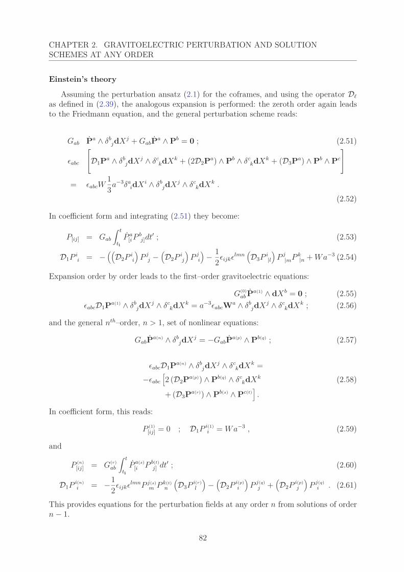
CHAPTER 2. GRAVITOELECTRIC PERTURBATION AND SOLUTIONSCHEMES AT ANY ORDER
Einstein’s theory
Assuming the perturbation ansatz (2.1) for the coframes, and using the operator D�
as defined in (2.39), the analogous expansion is performed: the zeroth order again leadsto the Friedmann equation, and the general perturbation scheme reads:
Gab Pa ∧ δbjdXj + GabPa ∧ Pb = 0 ; (2.51)
εabc
⎡⎣D1Pa ∧ δb
jdXj ∧ δckdXk + (2D2Pa) ∧ Pb ∧ δc
kdXk + (D3Pa) ∧ Pb ∧ Pc
⎤⎦
= εabcW13a−3δa
idX i ∧ δbjdXj ∧ δc
kdXk .
(2.52)
In coefficient form and integrating (2.51) they become:
P[ij] = Gab
∫ t
tiP a
[iPbj]dt′ ; (2.53)
D1Pii = −
((D2P
ii
)P j
j −(D2P
ij
)P j
i
)− 1
2εijkεlmn(D3P
i|l)
P j|mP k
|n + Wa−3 .(2.54)
Expansion order by order leads to the first–order gravitoelectric equations:
G(0)ab Pa(1) ∧ dXb = 0 ; (2.55)
εabcD1Pa(1) ∧ δbjdXj ∧ δc
kdXk = a−3εabcWa ∧ δbjdXj ∧ δc
kdXk ; (2.56)
and the general nth–order, n > 1, set of nonlinear equations:
GabPa(n) ∧ δbjdXj = −GabPa(p) ∧ Pb(q) ; (2.57)
εabcD1Pa(n) ∧ δbjdXj ∧ δc
kdXk =−εabc
[2 (D2Pa(p)) ∧ Pb(q) ∧ δc
kdXk (2.58)
+ (D3Pa(r)) ∧ Pb(s) ∧ Pc(t)]
.
In coefficient form, this reads:
P (1)[ij] = 0 ; D1P
i(1)i = Wa−3 , (2.59)
and
P (n)[ij] = G(r)
ab
∫ t
tiP a(s)
[i P b(t)j] dt′ ; (2.60)
D1Pi(n)i = −1
2εijkεlmnP j(s)m P k(t)
n
(D3P
i(r)l
)−(D2P
i(p)i
)P j(q)
j +(D2P
i(p)j
)P j(q)
i . (2.61)
This provides equations for the perturbation fields at any order n from solutions of ordern − 1.
82
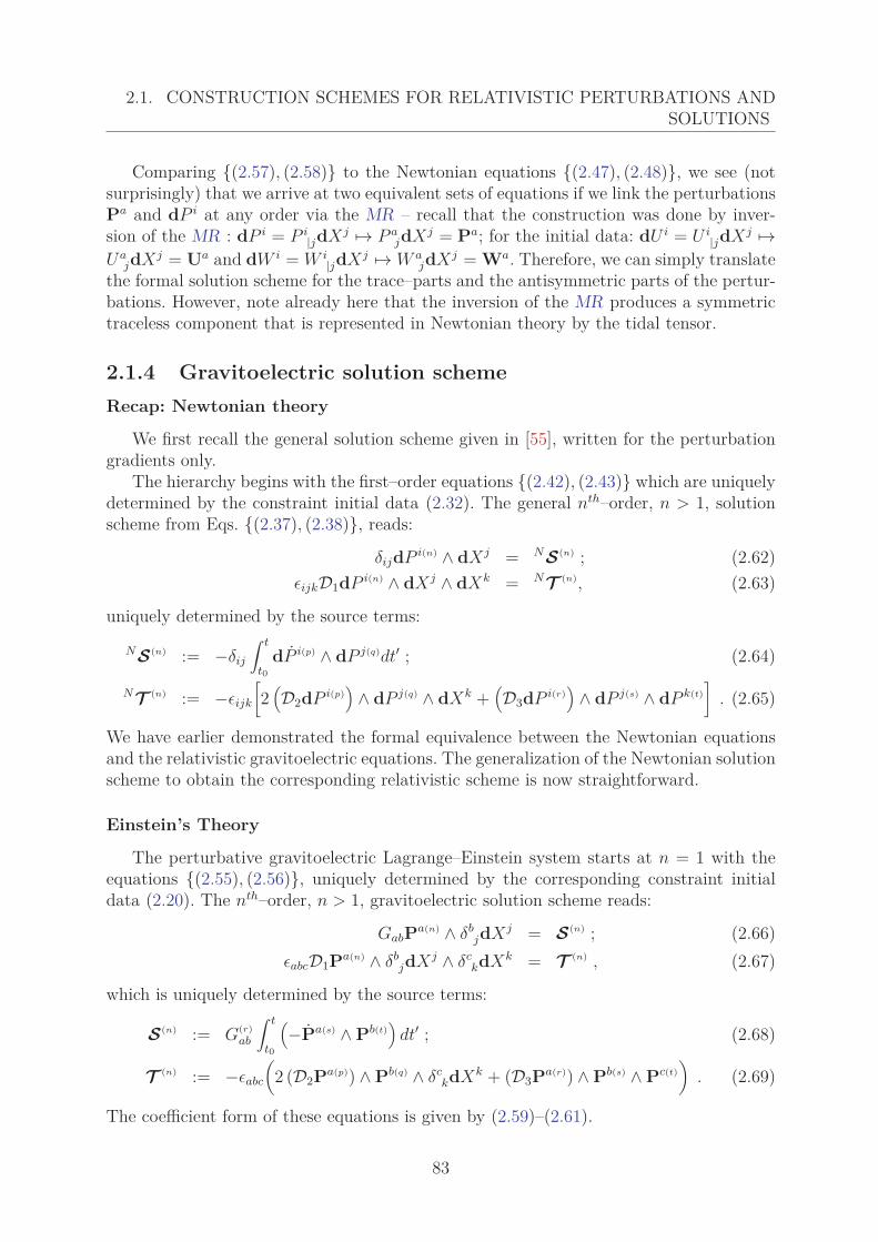
2.1. CONSTRUCTION SCHEMES FOR RELATIVISTIC PERTURBATIONS ANDSOLUTIONS
Comparing {(2.57), (2.58)} to the Newtonian equations {(2.47), (2.48)}, we see (notsurprisingly) that we arrive at two equivalent sets of equations if we link the perturbationsPa and dP i at any order via the MR – recall that the construction was done by inver-sion of the MR : dP i = P i
|jdXj → P ajdXj = Pa; for the initial data: dU i = U i
|jdXj →Ua
jdXj = Ua and dW i = W i|jdXj → W a
jdXj = Wa. Therefore, we can simply translatethe formal solution scheme for the trace–parts and the antisymmetric parts of the pertur-bations. However, note already here that the inversion of the MR produces a symmetrictraceless component that is represented in Newtonian theory by the tidal tensor.
2.1.4 Gravitoelectric solution schemeRecap: Newtonian theory
We first recall the general solution scheme given in [55], written for the perturbationgradients only.
The hierarchy begins with the first–order equations {(2.42), (2.43)} which are uniquelydetermined by the constraint initial data (2.32). The general nth–order, n > 1, solutionscheme from Eqs. {(2.37), (2.38)}, reads:
δijdP i(n) ∧ dXj = NS(n) ; (2.62)εijkD1dP i(n) ∧ dXj ∧ dXk = NT (n), (2.63)
uniquely determined by the source terms:
NS(n) := −δij
∫ t
t0dP i(p) ∧ dP j(q)dt′ ; (2.64)
NT (n) := −εijk
[2(D2dP i(p)
)∧ dP j(q) ∧ dXk +
(D3dP i(r)
)∧ dP j(s) ∧ dP k(t)
]. (2.65)
We have earlier demonstrated the formal equivalence between the Newtonian equationsand the relativistic gravitoelectric equations. The generalization of the Newtonian solutionscheme to obtain the corresponding relativistic scheme is now straightforward.
Einstein’s Theory
The perturbative gravitoelectric Lagrange–Einstein system starts at n = 1 with theequations {(2.55), (2.56)}, uniquely determined by the corresponding constraint initialdata (2.20). The nth–order, n > 1, gravitoelectric solution scheme reads:
GabPa(n) ∧ δbjdXj = S(n) ; (2.66)
εabcD1Pa(n) ∧ δbjdXj ∧ δc
kdXk = T (n) , (2.67)
which is uniquely determined by the source terms:
S(n) := G(r)ab
∫ t
t0
(−Pa(s) ∧ Pb(t)
)dt′ ; (2.68)
T (n) := −εabc
(2 (D2Pa(p)) ∧ Pb(q) ∧ δc
kdXk + (D3Pa(r)) ∧ Pb(s) ∧ Pc(t))
. (2.69)
The coefficient form of these equations is given by (2.59)–(2.61).
83
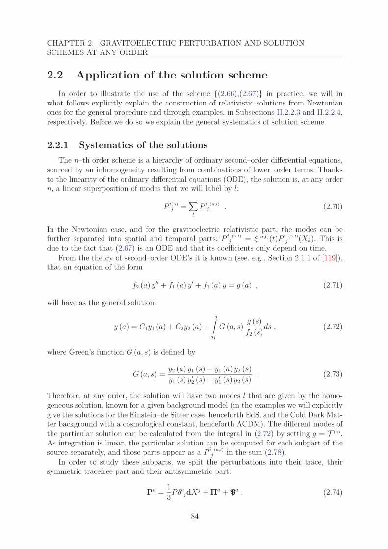
CHAPTER 2. GRAVITOELECTRIC PERTURBATION AND SOLUTIONSCHEMES AT ANY ORDER
2.2 Application of the solution schemeIn order to illustrate the use of the scheme {(2.66),(2.67)} in practice, we will in
what follows explicitly explain the construction of relativistic solutions from Newtonianones for the general procedure and through examples, in Subsections II.2.2.3 and II.2.2.4,respectively. Before we do so we explain the general systematics of solution scheme.
2.2.1 Systematics of the solutionsThe n–th order scheme is a hierarchy of ordinary second–order differential equations,
sourced by an inhomogeneity resulting from combinations of lower–order terms. Thanksto the linearity of the ordinary differential equations (ODE), the solution is, at any ordern, a linear superposition of modes that we will label by l:
P i(n)j =
∑l
P i (n,l)j . (2.70)
In the Newtonian case, and for the gravitoelectric relativistic part, the modes can befurther separated into spatial and temporal parts: P i (n,l)
j = ξ(n,l)(t)P i (n,l)j (Xk). This is
due to the fact that (2.67) is an ODE and that its coefficients only depend on time.From the theory of second–order ODE’s it is known (see, e.g., Section 2.1.1 of [119]),
that an equation of the form
f2 (a) y′′ + f1 (a) y′ + f0 (a) y = g (a) , (2.71)
will have as the general solution:
y (a) = C1y1 (a) + C2y2 (a) +a∫
ai
G (a, s) g (s)f2 (s)ds , (2.72)
where Green’s function G (a, s) is defined by
G (a, s) = y2 (a) y1 (s) − y1 (a) y2 (s)y1 (s) y′
2 (s) − y′1 (s) y2 (s) . (2.73)
Therefore, at any order, the solution will have two modes l that are given by the homo-geneous solution, known for a given background model (in the examples we will explicitlygive the solutions for the Einstein–de Sitter case, henceforth EdS, and the Cold Dark Mat-ter background with a cosmological constant, henceforth ΛCDM). The different modes ofthe particular solution can be calculated from the integral in (2.72) by setting g = T (n).As integration is linear, the particular solution can be computed for each subpart of thesource separately, and those parts appear as a P i (n,l)
j in the sum (2.78).In order to study these subparts, we split the perturbations into their trace, their
symmetric tracefree part and their antisymmetric part:
Pa = 13Pδa
jdXj + Πa + Pa . (2.74)
84
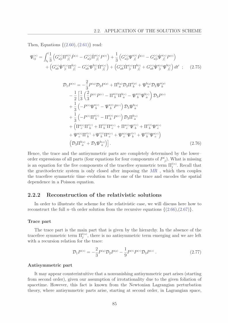
2.2. APPLICATION OF THE SOLUTION SCHEME
Then, Equations {(2.60), (2.61)} read:
P(n)ij =
∫ t
ti
13(G(r)
a[iΠa(t)j] P (s) − G(r)
a[iΠa(s)j] P (t)
)+ 1
3(G(r)
a[iPa(t)j] P (s) − G(r)
a[iPa(s)j] P (t)
)
+(G(r)
ab Pa(s)[i Πb(t)
j] − G(r)abP
b(t)[i Πa(s)
j]
)+(G(r)
ab Πa(s)[i Πb(t)
j] + G(r)ab P
a(s)[i P
b(t)j]
)dt′ ; (2.75)
D1P(n) = −2
3P (q)D2P(p) + Πb(q)
a D2Πa(p)b +Pb(q)
a D2Pa(p)b
− 12
[13
(23P (t)P (r) − Πa(t)
b Πb(r)a −Pa(t)
b Pb(r)a
)D3P
(s)
+ 13(−P (t)P
a(r)b −Pa(t)
b P (r))
D3Pb(s)a
+ 13(−P (t)Πa(r)
b − Πa(t)b P (r)
)D3Πb(s)
a
+(Πa(t)
c Πc(r)b + Πc(t)
b Πa(r)c + Πa(t)
c Pc(r)b + Πc(t)
b Pa(r)c
+Pa(t)c Πc(r)
b +Pc(t)b Πa(r)
c +Pa(t)c P
c(r)b +Pc(t)
b Pa(r)c
)(D3Πb(s)
a + D3Pb(s)a
)]. (2.76)
Hence, the trace and the antisymmetric parts are completely determined by the lower–order expressions of all parts (four equations for four components of P i
j). What is missingis an equation for the five components of the tracefree symmetric term Πi(n)
j . Recall thatthe gravitoelectric system is only closed after imposing the MR , which then couplesthe tracefree symmetric time–evolution to the one of the trace and encodes the spatialdependence in a Poisson equation.
2.2.2 Reconstruction of the relativistic solutionsIn order to illustrate the scheme for the relativistic case, we will discuss here how to
reconstruct the full n–th order solution from the recursive equations {(2.66),(2.67)}.
Trace part
The trace part is the main part that is given by the hierarchy. In the absence of thetracefree symmetric term Πi(n)
j , there is no antisymmetric term emerging and we are leftwith a recursion relation for the trace:
D1P(n) = −2
3P (q)D2P(p) − 1
9P (t)P (r)D3P(s) . (2.77)
Antisymmetric part
It may appear counterintuitive that a nonvanishing antisymmetric part arises (startingfrom second order), given our assumption of irrotationality due to the given foliation ofspacetime. However, this fact is known from the Newtonian Lagrangian perturbationtheory, where antisymmetric parts arise, starting at second order, in Lagrangian space,
85
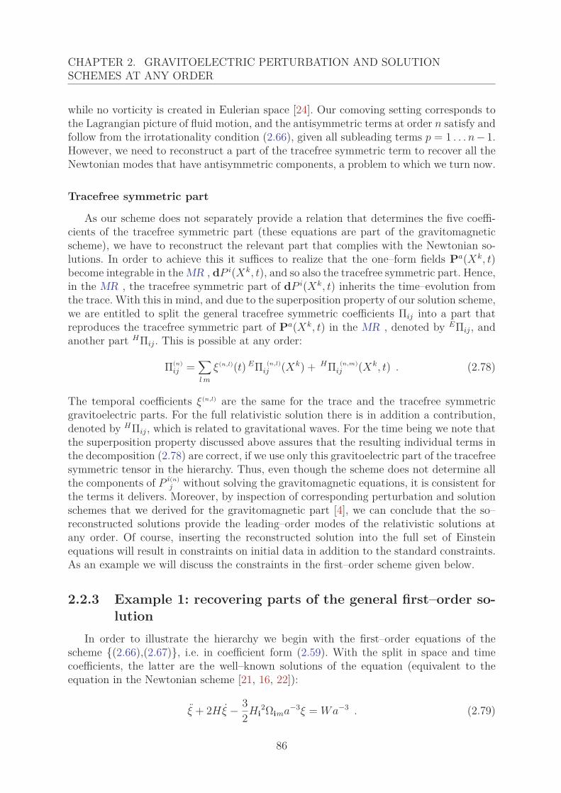
CHAPTER 2. GRAVITOELECTRIC PERTURBATION AND SOLUTIONSCHEMES AT ANY ORDER
while no vorticity is created in Eulerian space [24]. Our comoving setting corresponds tothe Lagrangian picture of fluid motion, and the antisymmetric terms at order n satisfy andfollow from the irrotationality condition (2.66), given all subleading terms p = 1 . . . n − 1.However, we need to reconstruct a part of the tracefree symmetric term to recover all theNewtonian modes that have antisymmetric components, a problem to which we turn now.
Tracefree symmetric part
As our scheme does not separately provide a relation that determines the five coeffi-cients of the tracefree symmetric part (these equations are part of the gravitomagneticscheme), we have to reconstruct the relevant part that complies with the Newtonian so-lutions. In order to achieve this it suffices to realize that the one–form fields Pa(Xk, t)become integrable in the MR , dP i(Xk, t), and so also the tracefree symmetric part. Hence,in the MR , the tracefree symmetric part of dP i(Xk, t) inherits the time–evolution fromthe trace. With this in mind, and due to the superposition property of our solution scheme,we are entitled to split the general tracefree symmetric coefficients Πij into a part thatreproduces the tracefree symmetric part of Pa(Xk, t) in the MR , denoted by EΠij, andanother part HΠij. This is possible at any order:
Π(n)ij =
∑l m
ξ(n,l)(t) EΠ (n,l)ij (Xk) + HΠ (n,m)
ij (Xk, t) . (2.78)
The temporal coefficients ξ(n,l) are the same for the trace and the tracefree symmetricgravitoelectric parts. For the full relativistic solution there is in addition a contribution,denoted by HΠij, which is related to gravitational waves. For the time being we note thatthe superposition property discussed above assures that the resulting individual terms inthe decomposition (2.78) are correct, if we use only this gravitoelectric part of the tracefreesymmetric tensor in the hierarchy. Thus, even though the scheme does not determine allthe components of P i(n)
j without solving the gravitomagnetic equations, it is consistent forthe terms it delivers. Moreover, by inspection of corresponding perturbation and solutionschemes that we derived for the gravitomagnetic part [4], we can conclude that the so–reconstructed solutions provide the leading–order modes of the relativistic solutions atany order. Of course, inserting the reconstructed solution into the full set of Einsteinequations will result in constraints on initial data in addition to the standard constraints.As an example we will discuss the constraints in the first–order scheme given below.
2.2.3 Example 1: recovering parts of the general first–order so-lution
In order to illustrate the hierarchy we begin with the first–order equations of thescheme {(2.66),(2.67)}, i.e. in coefficient form (2.59). With the split in space and timecoefficients, the latter are the well–known solutions of the equation (equivalent to theequation in the Newtonian scheme [21, 16, 22]):
ξ + 2Hξ − 32Hi
2Ωima−3ξ = Wa−3 . (2.79)
86
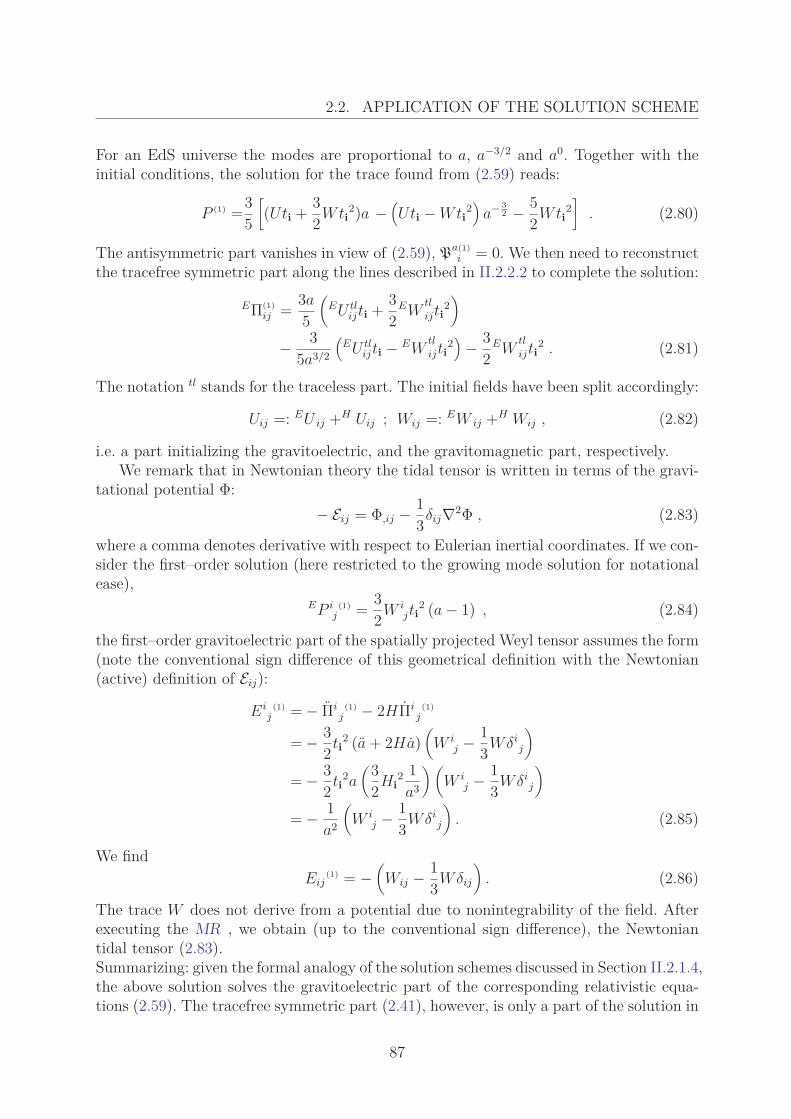
2.2. APPLICATION OF THE SOLUTION SCHEME
For an EdS universe the modes are proportional to a, a−3/2 and a0. Together with theinitial conditions, the solution for the trace found from (2.59) reads:
P (1) =35
[(Uti + 3
2Wti2)a −
(Uti − Wti
2)
a− 32 − 5
2Wti2]
. (2.80)
The antisymmetric part vanishes in view of (2.59), Pa(1)i = 0. We then need to reconstruct
the tracefree symmetric part along the lines described in II.2.2.2 to complete the solution:
EΠ(1)ij = 3a
5
(EU tl
ijti + 32
EWtl
ijti2)
− 35a3/2
(EU tl
ijti − EWtl
ijti2)
− 32
EWtl
ijti2 . (2.81)
The notation tl stands for the traceless part. The initial fields have been split accordingly:
Uij =: EU ij +H Uij ; Wij =: EW ij +H Wij , (2.82)
i.e. a part initializing the gravitoelectric, and the gravitomagnetic part, respectively.We remark that in Newtonian theory the tidal tensor is written in terms of the gravi-
tational potential Φ:− Eij = Φ,ij − 1
3δij∇2Φ , (2.83)
where a comma denotes derivative with respect to Eulerian inertial coordinates. If we con-sider the first–order solution (here restricted to the growing mode solution for notationalease),
EP ij
(1) = 32W i
jti2 (a − 1) , (2.84)
the first–order gravitoelectric part of the spatially projected Weyl tensor assumes the form(note the conventional sign difference of this geometrical definition with the Newtonian(active) definition of Eij):
Eij
(1) = − Πij
(1) − 2HΠij
(1)
= − 32ti
2 (a + 2Ha)(
W ij − 1
3Wδij
)
= − 32ti
2a(3
2Hi2 1a3
)(W i
j − 13Wδi
j
)
= − 1a2
(W i
j − 13Wδi
j
). (2.85)
We findEij
(1) = −(
Wij − 13Wδij
). (2.86)
The trace W does not derive from a potential due to nonintegrability of the field. Afterexecuting the MR , we obtain (up to the conventional sign difference), the Newtoniantidal tensor (2.83).Summarizing: given the formal analogy of the solution schemes discussed in Section II.2.1.4,the above solution solves the gravitoelectric part of the corresponding relativistic equa-tions (2.59). The tracefree symmetric part (2.41), however, is only a part of the solution in
87
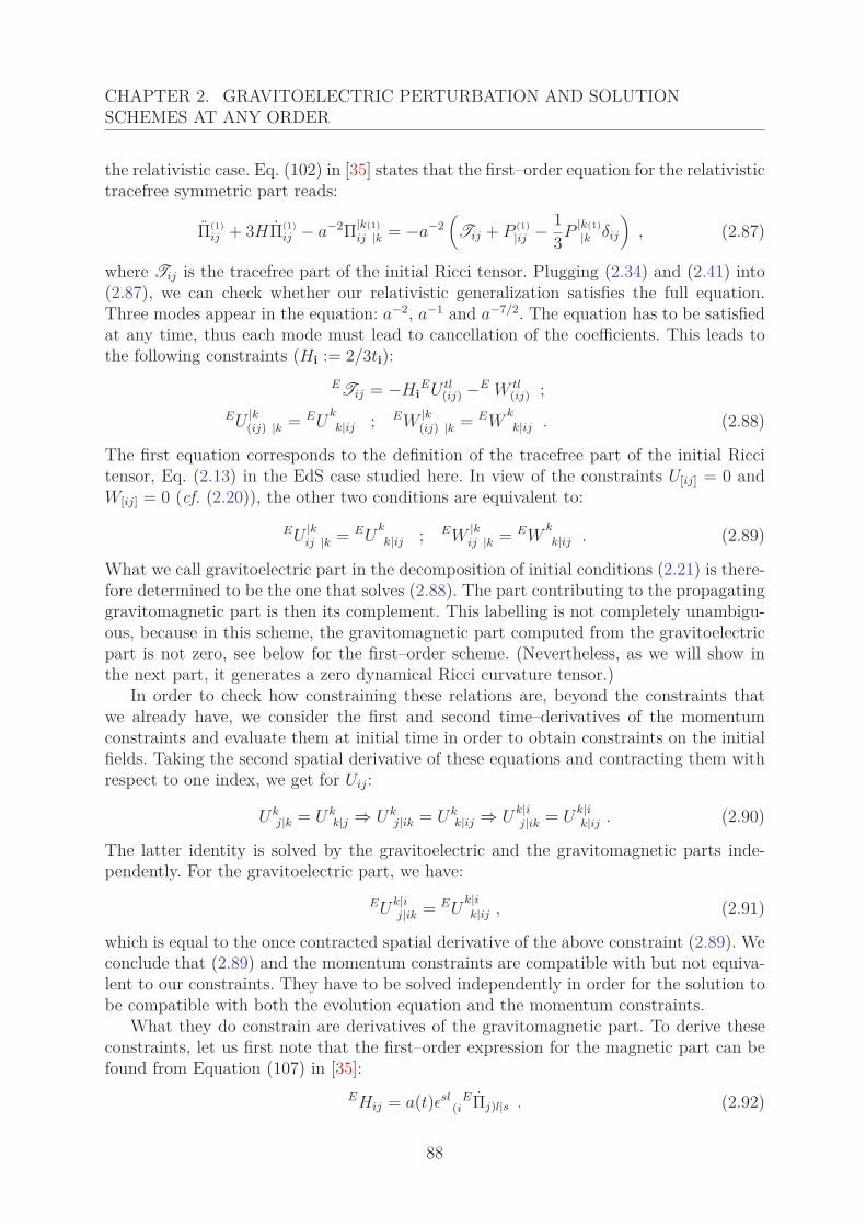
CHAPTER 2. GRAVITOELECTRIC PERTURBATION AND SOLUTIONSCHEMES AT ANY ORDER
the relativistic case. Eq. (102) in [35] states that the first–order equation for the relativistictracefree symmetric part reads:
Π(1)ij + 3HΠ(1)
ij − a−2Π|k(1)ij |k = −a−2
(Tij + P (1)
|ij − 13P
|k(1)|k δij
), (2.87)
where Tij is the tracefree part of the initial Ricci tensor. Plugging (2.34) and (2.41) into(2.87), we can check whether our relativistic generalization satisfies the full equation.Three modes appear in the equation: a−2, a−1 and a−7/2. The equation has to be satisfiedat any time, thus each mode must lead to cancellation of the coefficients. This leads tothe following constraints (Hi := 2/3ti):
ETij = −HiEU tl
(ij) −E W tl(ij) ;
EU|k(ij) |k = EU
k
k|ij ; EW|k(ij) |k = EW
k
k|ij . (2.88)
The first equation corresponds to the definition of the tracefree part of the initial Riccitensor, Eq. (2.13) in the EdS case studied here. In view of the constraints U[ij] = 0 andW[ij] = 0 (cf. (2.20)), the other two conditions are equivalent to:
EU|kij |k = EU
k
k|ij ; EW|kij |k = EW
k
k|ij . (2.89)
What we call gravitoelectric part in the decomposition of initial conditions (2.21) is there-fore determined to be the one that solves (2.88). The part contributing to the propagatinggravitomagnetic part is then its complement. This labelling is not completely unambigu-ous, because in this scheme, the gravitomagnetic part computed from the gravitoelectricpart is not zero, see below for the first–order scheme. (Nevertheless, as we will show inthe next part, it generates a zero dynamical Ricci curvature tensor.)
In order to check how constraining these relations are, beyond the constraints thatwe already have, we consider the first and second time–derivatives of the momentumconstraints and evaluate them at initial time in order to obtain constraints on the initialfields. Taking the second spatial derivative of these equations and contracting them withrespect to one index, we get for Uij:
Ukj|k = Uk
k|j ⇒ Ukj|ik = Uk
k|ij ⇒ Uk|ij|ik = U
k|ik|ij . (2.90)
The latter identity is solved by the gravitoelectric and the gravitomagnetic parts inde-pendently. For the gravitoelectric part, we have:
EUk|ij|ik = EU
k|ik|ij , (2.91)
which is equal to the once contracted spatial derivative of the above constraint (2.89). Weconclude that (2.89) and the momentum constraints are compatible with but not equiva-lent to our constraints. They have to be solved independently in order for the solution tobe compatible with both the evolution equation and the momentum constraints.
What they do constrain are derivatives of the gravitomagnetic part. To derive theseconstraints, let us first note that the first–order expression for the magnetic part can befound from Equation (107) in [35]:
EHij = a(t)εsl(i
EΠj)l|s . (2.92)
88
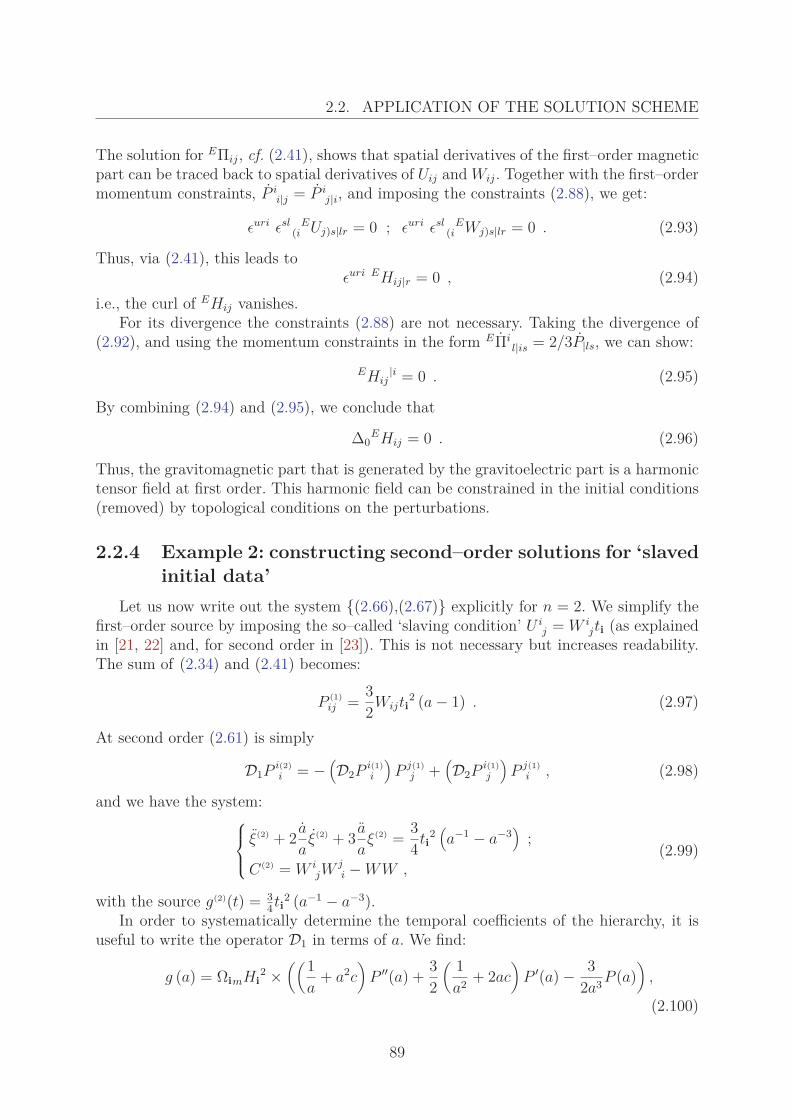
2.2. APPLICATION OF THE SOLUTION SCHEME
The solution for EΠij, cf. (2.41), shows that spatial derivatives of the first–order magneticpart can be traced back to spatial derivatives of Uij and Wij. Together with the first–ordermomentum constraints, P i
i|j = P ij|i, and imposing the constraints (2.88), we get:
εuri εsl(i
EUj)s|lr = 0 ; εuri εsl(i
EWj)s|lr = 0 . (2.93)
Thus, via (2.41), this leads toεuri EHij|r = 0 , (2.94)
i.e., the curl of EHij vanishes.For its divergence the constraints (2.88) are not necessary. Taking the divergence of
(2.92), and using the momentum constraints in the form EΠil|is = 2/3P|ls, we can show:
EHij|i = 0 . (2.95)
By combining (2.94) and (2.95), we conclude that
Δ0EHij = 0 . (2.96)
Thus, the gravitomagnetic part that is generated by the gravitoelectric part is a harmonictensor field at first order. This harmonic field can be constrained in the initial conditions(removed) by topological conditions on the perturbations.
2.2.4 Example 2: constructing second–order solutions for ‘slavedinitial data’
Let us now write out the system {(2.66),(2.67)} explicitly for n = 2. We simplify thefirst–order source by imposing the so–called ‘slaving condition’ U i
j = W ijti (as explained
in [21, 22] and, for second order in [23]). This is not necessary but increases readability.The sum of (2.34) and (2.41) becomes:
P (1)ij = 3
2Wijti2 (a − 1) . (2.97)
At second order (2.61) is simply
D1Pi(2)i = −
(D2P
i(1)i
)P j(1)
j +(D2P
i(1)j
)P j(1)
i , (2.98)
and we have the system:⎧⎪⎨⎪⎩
ξ(2) + 2 a
aξ(2) + 3 a
aξ(2) = 3
4ti2(a−1 − a−3
);
C(2) = W ijW
ji − WW ,
(2.99)
with the source g(2)(t) = 34ti
2 (a−1 − a−3).In order to systematically determine the temporal coefficients of the hierarchy, it is
useful to write the operator D1 in terms of a. We find:
g (a) = ΩimHi2 ×
((1a
+ a2c)
P ′′(a) + 32
( 1a2 + 2ac
)P ′(a) − 3
2a3 P (a))
,
(2.100)
89
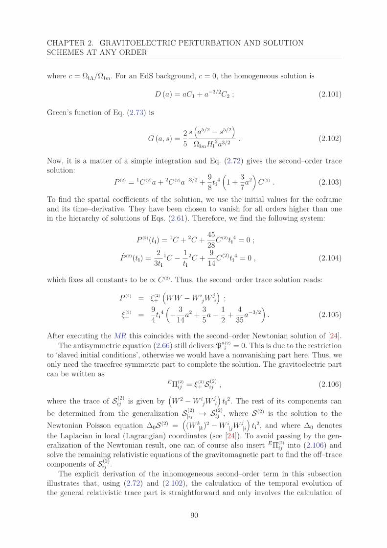
CHAPTER 2. GRAVITOELECTRIC PERTURBATION AND SOLUTIONSCHEMES AT ANY ORDER
where c = ΩiΛ/Ωim. For an EdS background, c = 0, the homogeneous solution is
D (a) = aC1 + a−3/2C2 ; (2.101)
Green’s function of Eq. (2.73) is
G (a, s) = 25
s(a5/2 − s5/2
)ΩimHi
2a3/2 . (2.102)
Now, it is a matter of a simple integration and Eq. (2.72) gives the second–order tracesolution:
P (2) = 1C(2)a + 2C(2)a−3/2 + 98ti
4(
1 + 37a2
)C(2) . (2.103)
To find the spatial coefficients of the solution, we use the initial values for the coframeand its time–derivative. They have been chosen to vanish for all orders higher than onein the hierarchy of solutions of Eqs. (2.61). Therefore, we find the following system:
P (2)(ti) = 1C + 2C + 4528C(2)ti
4 = 0 ;
P (2)(ti) = 23ti
1C − 1ti
2C + 914C(2)ti
4 = 0 , (2.104)
which fixes all constants to be ∝ C(2). Thus, the second–order trace solution reads:
P (2) = ξ(2)+(WW − W i
jWji
);
ξ(2)+ = 9
4ti4(
− 314a2 + 3
5a − 12 + 4
35a−3/2)
. (2.105)
After executing the MR this coincides with the second–order Newtonian solution of [24].The antisymmetric equation (2.66) still delivers Pa(2)
i = 0. This is due to the restrictionto ‘slaved initial conditions’, otherwise we would have a nonvanishing part here. Thus, weonly need the tracefree symmetric part to complete the solution. The gravitoelectric partcan be written as
EΠ(2)ij = ξ(2)
+ S(2)ij , (2.106)
where the trace of S(2)ij is given by
(W 2 − W i
jWji
)ti
2. The rest of its components canbe determined from the generalization S(2)
|ij → S(2)ij , where S(2) is the solution to the
Newtonian Poisson equation Δ0S(2) =((W k
|k)2 − W i|jW
j|i)
ti2, and where Δ0 denotes
the Laplacian in local (Lagrangian) coordinates (see [24]). To avoid passing by the gen-eralization of the Newtonian result, one can of course also insert EΠ(2)
ij into (2.106) andsolve the remaining relativistic equations of the gravitomagnetic part to find the off–tracecomponents of S(2)
ij .The explicit derivation of the inhomogeneous second–order term in this subsection
illustrates that, using (2.72) and (2.102), the calculation of the temporal evolution ofthe general relativistic trace part is straightforward and only involves the calculation of
90
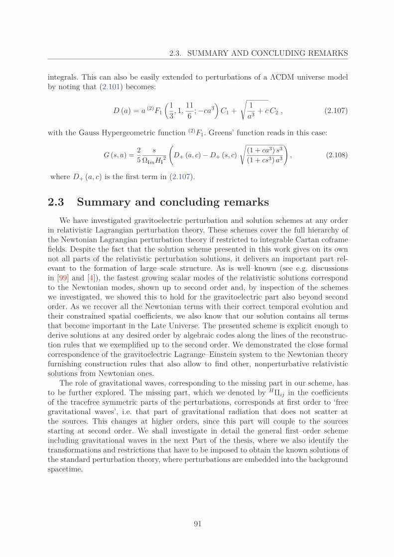
2.3. SUMMARY AND CONCLUDING REMARKS
integrals. This can also be easily extended to perturbations of a ΛCDM universe modelby noting that (2.101) becomes:
D (a) = a (2)F1
(13 , 1,
116 ; −ca3
)C1 +
√1a3 + c C2 , (2.107)
with the Gauss Hypergeometric function (2)F1. Greens’ function reads in this case:
G (s, a) =25
s
ΩimHi2
(D+ (a, c) − D+ (s, c)
√(1 + ca3) s3
(1 + cs3) a3
), (2.108)
where D+ (a, c) is the first term in (2.107).
2.3 Summary and concluding remarksWe have investigated gravitoelectric perturbation and solution schemes at any order
in relativistic Lagrangian perturbation theory. These schemes cover the full hierarchy ofthe Newtonian Lagrangian perturbation theory if restricted to integrable Cartan coframefields. Despite the fact that the solution scheme presented in this work gives on its ownnot all parts of the relativistic perturbation solutions, it delivers an important part rel-evant to the formation of large–scale structure. As is well–known (see e.g. discussionsin [99] and [4]), the fastest growing scalar modes of the relativistic solutions correspondto the Newtonian modes, shown up to second order and, by inspection of the schemeswe investigated, we showed this to hold for the gravitoelectric part also beyond secondorder. As we recover all the Newtonian terms with their correct temporal evolution andtheir constrained spatial coefficients, we also know that our solution contains all termsthat become important in the Late Universe. The presented scheme is explicit enough toderive solutions at any desired order by algebraic codes along the lines of the reconstruc-tion rules that we exemplified up to the second order. We demonstrated the close formalcorrespondence of the gravitoelectric Lagrange–Einstein system to the Newtonian theoryfurnishing construction rules that also allow to find other, nonperturbative relativisticsolutions from Newtonian ones.
The role of gravitational waves, corresponding to the missing part in our scheme, hasto be further explored. The missing part, which we denoted by HΠij in the coefficientsof the tracefree symmetric parts of the perturbations, corresponds at first order to ‘freegravitational waves’, i.e. that part of gravitational radiation that does not scatter atthe sources. This changes at higher orders, since this part will couple to the sourcesstarting at second order. We shall investigate in detail the general first–order schemeincluding gravitational waves in the next Part of the thesis, where we also identify thetransformations and restrictions that have to be imposed to obtain the known solutions ofthe standard perturbation theory, where perturbations are embedded into the backgroundspacetime.
91
Part III
From a Local to a GlobalDescription of First-Order
Intrinsic Lagrangian Perturbations
92

Chapter 1
Gravitational Waves in the StandardPerturbation Theory
Contents1.1 Propagative dynamics in the intrinsic approach: motivations
and strategy . . . . . . . . . . . . . . . . . . . . . . . . . . . . . 951.2 Standard description of gravitational waves . . . . . . . . . . . 96
1.2.1 Observing gravitational waves in the Standard Perturbation The-ory . . . . . . . . . . . . . . . . . . . . . . . . . . . . . . . . . . 96
1.2.2 Linearizing the Einstein equations . . . . . . . . . . . . . . . . 961.2.3 Gravitoelectromagnetism in the weak field limit . . . . . . . . . 981.2.4 Plane gravitational waves and polarization . . . . . . . . . . . . 98
94
1.1 Propagative dynamics in the intrinsic approach:motivations and strategy
In the last part we have used the formal analogy between the gravitoelectric part ofthe Einstein equations and the Lagrange-Newton-System to build a relativistic general-ization of the Newtonian perturbative solution to order n. These solutions exhibit thesame time-dependence as the Newtonian ones and therefore do not encode propagativedynamics. Furthermore, we have seen that, at first-order, the gravitoelectric part of theinitial conditions has to fulfill the equalities (2.89). As discussed in Section II.1.4.3, themagnetic part of the Weyl tensor is often thought to encode gravitational waves. It isinteresting to note that the gravitoelectric solutions also generate a magnetic part thatonly at first order is a solution of the Laplace equation (2.96). These equations are ellipticand thus need boundary conditions to be solved. In General Relativity, if we are lookingfor a global solution on the manifold, these boundary conditions are provided by topology.
In this part, we will consider only the first-order perturbation theory. Gravitationalwaves have then only a trivial component in the gravitoelectric class of solutions. We willtherefore determine where and how they are encoded in the complementary part of thesolution obtained from the Newtonian perturbation theory. Moreover, we will compareour intrinsic Lagrangian perturbative approach to the standard perturbation theory, inorder to highlight the similarities and identify the differences between the two. One of themain issues will be to understand under which conditions the gravitoelectric part of thesolution represents the integrable part of the perturbation fields.
In the following chapter, we begin with a short presentation of the standard theoryof gravitational waves. We will present the instruments that have been built to detectthem and explain how they have been theoretically predicted from the linearization ofthe Einstein equations. Furthermore, we will discuss the gravitoelectromagnetic analogyfor the linearized Einstein equations in the weak field limit. The standard treatment ofgravitational waves is presented in order to better understand why our description goesbeyond the standard approach, even at first-order.
The second chapter will focus on the local first-order Einstein equations and solutions.We will give the first results on the gravitomagnetic part of the solution and will carry outa comparison to the standard perturbative approach. The last chapter will treat globallythe coframes and the spatial manifold. Some powerful mathematical tools and theorems,available for closed topological spaces, will be used to determine the impact of topologyon the first-order solutions.
95
CHAPTER 1. GRAVITATIONAL WAVES IN THE STANDARD PERTURBATIONTHEORY
1.2 Standard description of gravitational waves
1.2.1 Observing gravitational waves in the Standard Perturba-tion Theory
Gravitational waves were predicted by Albert Einstein [60] and are a natural conse-quence of General Relativity. They propagate at the speed of light, such as the electro-magnetic waves but, contrary to the electromagnetic waves, they do not propagate onspace-time but are a propagating oscillation of space-time itself. Measures of time andlength are thus modified by gravitational waves. Nevertheless, these effects are very smalland the sensitivity of the detectors should be higher then the current one.
Indeed, being an interferometer on Earth, Virgo uses the modification of lengths bygravitational waves to detect them. A great amount of the noise in its measurements isdue to some local vibrations. Overcoming this intrinsic limit is a true technical prowess.However, Virgo has not detected gravitational waves so far.
Measuring the polarization of the CMB, the BICEP 2 (Background Imaging of CosmicExtragalactic Polarization) experiment, located in the Antarctic Amundsen-Scott base inthe South Pole, claimed to have found primordial gravitational waves. Data from theBICEP2 telescope and Planck were analyzed jointly. It turned out that the signal couldbe entirely attributed to dust in the Milky Way rather than to the signature of someprimordial gravitational waves [47].
The eLISA spatial gravitational wave detector https://www.elisascience.org ,which will be the European Space Agency focus for the next two large science missions,will be a huge improvement for detection of gravitational waves. Measuring gravitationalwaves will not only confirm one of the predictions of General Relativity, it will further-more provide us with some precious information in some aspects of cosmology such as theEarly Universe or the large scale structure formation.
For some very good lectures on gravitational waves, the reader can refer to [73], [152]and [74].
In order to better compare our Lagrangian perturbation approach to the standardone, I here present how equations for propagation of gravitational waves are derived whenthe metric tensor is perturbed around a Minkowski background. Furthermore, since oneof the important aspects of my research is gravitoelectromagnetism, I wish to discusshow, from the standard linearized Einstein equations, we can obtain the analogue of theMaxwell equations and even the Lorentz force. In order to simplify the comparison toelectromagnetism, we will not use the c = 1 units in this section.
1.2.2 Linearizing the Einstein equationsWhen we linearize the Einstein equations according to (1.1), the gravitational field is
weak, but it doesn’t have to be static, and particles are allowed to move with relativisticvelocities.
We will consider small perturbations around a Minkowski space-time. The metrictensor will then be decomposed as:
gμν = ημν + hμν ; |hμν | � 1 , (1.1)
96
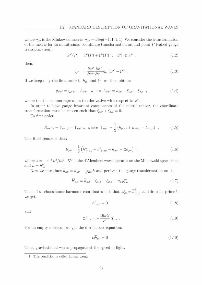
1.2. STANDARD DESCRIPTION OF GRAVITATIONAL WAVES
where ημν is the Minkowski metric: ημν = diag(−1, 1, 1, 1). We consider the transformationof the metric for an infinitesimal coordinate transformation around point P (called gaugetransformation):
xμ′(P ) = xμ(P ) + ξμ(P ) ; |ξμ| � xμ , (1.2)
then,
gρ′σ′ = ∂xμ
∂xρ′∂xν
∂xσ′ gμν(xμ′ − ξμ) . (1.3)
If we keep only the first–order in hμν and ξμ, we then obtain:
gρ′σ′ = ηρ′σ′ + hρ′σ′ where hρ′σ′ = hρσ − ξρ,σ − ξσ,ρ , (1.4)
where the the comma represents the derivative with respect to xμ.In order to have gauge invariant components of the metric tensor, the coordinate
transformation must be chosen such that ξρ,σ + ξσ,ρ = 0.To first order,
Rαμβν = Γαμν,β − Γαμβ,ν where Γαμν = 12 (hμα,ν + hνα,μ − hμν,α) . (1.5)
The Ricci tensor is thus:
Rμν = 12(hα
ν,αμ + hαμ,αν − h,μν − �hμν
), (1.6)
where � = −c−2 ∂2/∂t2+∇2 is the d’Alembert wave operator on the Minkowski space-timeand h = hα
α.Now we introduce hμν = hμν − 1
2ημνh and perform the gauge transformation on it.
h′αβ = hαβ − ξα,β − ξβ,α + ηαβξσ
σ . (1.7)
Then, if we choose some harmonic coordinates such that �ξα = hβ
α,β, and drop the prime 1,we get:
hβ
α,β = 0 , (1.8)
and�hμν = −16πG
c4 Tμν . (1.9)
For an empty universe, we get the d’Alembert equation:
�hμν = 0 . (1.10)
Thus, gravitational waves propagate at the speed of light.
1. This condition is called Lorenz gauge
97
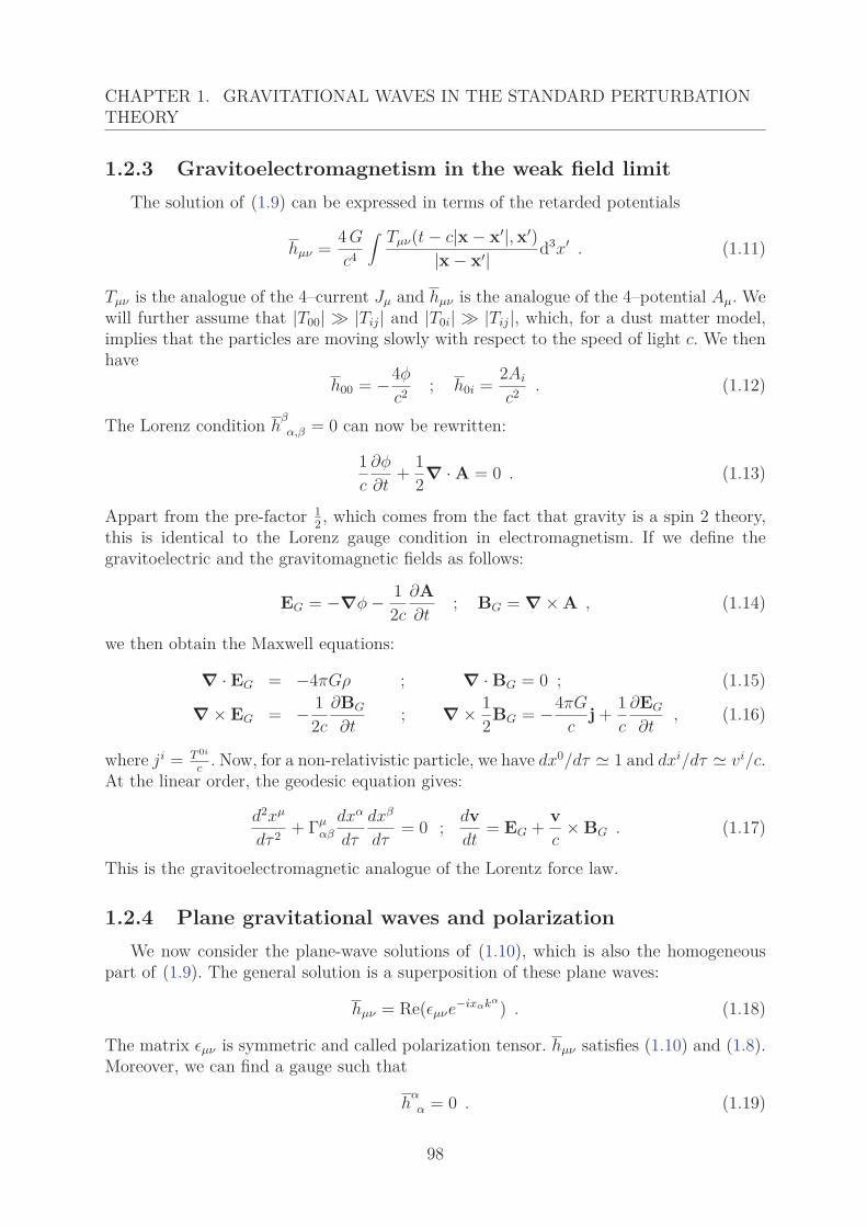
CHAPTER 1. GRAVITATIONAL WAVES IN THE STANDARD PERTURBATIONTHEORY
1.2.3 Gravitoelectromagnetism in the weak field limitThe solution of (1.9) can be expressed in terms of the retarded potentials
hμν = 4 G
c4
∫ Tμν(t − c|x − x′|, x′)|x − x′| d3x′ . (1.11)
Tμν is the analogue of the 4–current Jμ and hμν is the analogue of the 4–potential Aμ. Wewill further assume that |T00| � |Tij| and |T0i| � |Tij|, which, for a dust matter model,implies that the particles are moving slowly with respect to the speed of light c. We thenhave
h00 = −4φ
c2 ; h0i = 2Ai
c2 . (1.12)
The Lorenz condition hβ
α,β = 0 can now be rewritten:
1c
∂φ
∂t+ 1
2∇ · A = 0 . (1.13)
Appart from the pre-factor 12 , which comes from the fact that gravity is a spin 2 theory,
this is identical to the Lorenz gauge condition in electromagnetism. If we define thegravitoelectric and the gravitomagnetic fields as follows:
EG = −∇φ − 12c
∂A∂t
; BG = ∇ × A , (1.14)
we then obtain the Maxwell equations:
∇ · EG = −4πGρ ; ∇ · BG = 0 ; (1.15)
∇ × EG = − 12c
∂BG
∂t; ∇ × 1
2BG = −4πG
cj + 1
c
∂EG
∂t, (1.16)
where ji = T 0i
c. Now, for a non-relativistic particle, we have dx0/dτ � 1 and dxi/dτ � vi/c.
At the linear order, the geodesic equation gives:
d2xμ
dτ 2 + Γμαβ
dxα
dτ
dxβ
dτ= 0 ; dv
dt= EG + v
c× BG . (1.17)
This is the gravitoelectromagnetic analogue of the Lorentz force law.
1.2.4 Plane gravitational waves and polarizationWe now consider the plane-wave solutions of (1.10), which is also the homogeneous
part of (1.9). The general solution is a superposition of these plane waves:
hμν = Re(εμνe−ixαkα) . (1.18)
The matrix εμν is symmetric and called polarization tensor. hμν satisfies (1.10) and (1.8).Moreover, we can find a gauge such that
hα
α = 0 . (1.19)
98
1.2. STANDARD DESCRIPTION OF GRAVITATIONAL WAVES
Figure 1.1: Motion of test particles for two linearly polarized states.
This implies the following relations for the wave vector and polarization tensor:
kαkα = 0 ; kαεαβ = 0 ; εαα = 0 . (1.20)
The initially 10 degrees of freedom for εμν become 5. The other three can be eliminatedusing the additional gauge transformations in the class of the harmonic coordinates. Tobe compatible with (1.8) and (1.19), such a coordinate transformation must satisfy
�ξα = 0 ; ξα,α = 0 . (1.21)
For this gauge class, we have hμν = hμν . We can choose ξα = Re(iεα exp (ikαxα)), thepolarization tensor in the new coordinates becomes
ε′μν = εμν + kμεν + kνεμ . (1.22)
ε′μν and εμν represent the same physical situation for any value of εν . If we consider
a propagation in the z− direction, then kμ = (k, 0, 0, k), we can show, combining thedifferent equalities (1.20), that one can choose εα such that only ε12 and ε11 = −ε22 donot vanish. Thus only two degrees of freedom are left: the two possible polarizations forgravitational waves. Figure 1.1 represents, for two linearly polarized states, the motionof test particles moving about a central particle in the transverse plane. For a completeintroduction on gravitational waves, the reader can refer to [152, 74, 138].
99
Chapter 2
Local Approach to First-OrderSolutions
Contents2.1 Local approach and propagative dynamics . . . . . . . . . . . 1012.2 First–order perturbation scheme in a local approach . . . . . 102
2.2.1 First–order perturbation scheme . . . . . . . . . . . . . . . . . 102Homogeneous equations . . . . . . . . . . . . . . . . . . . . . . 102
2.2.2 First–order equations . . . . . . . . . . . . . . . . . . . . . . . 1032.2.3 First–order master equations . . . . . . . . . . . . . . . . . . . 105
Splitting of the solution into EΠij and HΠij . . . . . . . . . . . 106Contributions of EΠij and HΠij to the Ricci curvature . . . . . 107
2.3 Electric and magnetic spatial parts of the Weyl tensor andthe Maxwell-Weyl equations . . . . . . . . . . . . . . . . . . . . 107
2.3.1 Link to the electric and magnetic part of Weyl tensor . . . . . 107Gravitomagnetic part from EPij . . . . . . . . . . . . . . . . . 107Magnetic part of the Weyl tensor and deviations from flatness 107
2.4 Comparison with the other perturbation schemes . . . . . . . 1082.4.1 Non–propagating solutions for the intrinsic Lagrangian description108
Integrable and non-integrable initial conditions . . . . . . . . . 108Non–propagating separable modes . . . . . . . . . . . . . . . . 108Einstein–de Sitter background . . . . . . . . . . . . . . . . . . 109
2.4.2 Propagative behavior of the non–integrable part . . . . . . . . 109Particular solution for the non–integrable part . . . . . . . . . 109Monochromatic solution . . . . . . . . . . . . . . . . . . . . . . 109Minkowski Restriction and conclusions . . . . . . . . . . . . . . 110
2.4.3 Comparison to other perturbation schemes . . . . . . . . . . . 110S–V–T decomposition in the comoving synchronous gauge . . . 111Relating formally the two descriptions . . . . . . . . . . . . . . 112Identification of the integrable and the non-integrable part . . 113
2.5 Conclusions and limits of the local description . . . . . . . . . 113
100
In [4], the Lagrangian approach to General Relativity was proven to be powerfulto extract from the full solution of Einstein equation the part that has the same timedependence as the Newtonian solution. This was done in the frame of perturbation theory.In this part, we will go beyond the gravitoelectric part of the Einstein equations andconsider the full set of equations up to first–order. The Cartan formalism, in the frame ofthe intrinsic Lagrangian approach, will be the appropriate formalism to grasp the majorfeatures of the perturbative solutions.
As we will show, the first–order gravitoelectric part of the solution, built from theNewtonian perturbative solution, does not contribute dynamically to the curvature ofspace sections. Its complementary part will be the one containing the free gravitationalwaves.
One of the main tasks of this work will be to link the standard approach to ourperturbative description. We will show that, when we apply the MR on the first-orderperturbative solution, we will get back the scalar modes of the standard approach. Never-theless, the non-integrable first-order coframes we consider live on the perturbed manifoldwhereas in the standard perturbation theory, they are defined on the background spacesection. Therefore, the 0th order space, which we will call by convenience background, willnot play the same role as the background manifold, on which quantities are defined instandard perturbation theory.
Since our intrinsic approach is on curved space-times, we have to replace the Scalar-Vector-Tensor decomposition considered in the standard perturbation approach, and onlyavailable on flat space sections, by a decomposition that takes into account the geometryand topology of space. This will be done in the third chapter of this part.
2.1 Local approach and propagative dynamicsThe content of this part is mostly based on the article that will be published by Al
Roumi, Buchert and Wiegand. We will focus on the first–order perturbation equationsand solutions and try to understand what is the physical content of the complementarypart of the first–order solution obtained in [4], which is the relativistic counterpart of thefirst–order Newtonian solution.
We will show that the complementary part contains the first–order free gravitationalwaves. Moreover, we will interpret the first–order results in terms of electric and magneticparts of Weyl tensor, which are solutions of equations that are formally analogue toMaxwell’s equations (cf Section II.1.4.3). Moreover, we will see that the formalism usedin [4] is implicitly local. In the next chapter, we will do assumptions on the topology ofspatial sections in order to draw from local results some global conclusions. This localapproach will enable us to compare our description to the standard one, since, in thestandard perturbation theory, quantities are defined on a flat background. In this frame,Green theory can be used to build global solutions.
In this chapter, we wish first to understand the physical contents of the complementarypart of the solution obtained from the Newtonian perturbation scheme. Then, we willshow that the local description may hinder a full comprehension of the dynamics of theperturbation fields. To efficiently overcome the limits of the local approach, a global
101
CHAPTER 2. LOCAL APPROACH TO FIRST-ORDER SOLUTIONS
description will have to be considered. This will be the topic of the next chapter.
2.2 First–order perturbation scheme in a local ap-proach
2.2.1 First–order perturbation schemeThe general perturbation scheme in the Intrinsic Lagrangian approach has been pre-
sented in Section II.2.1.1 to any order. From now on, we only consider first–order devia-tions. Thus, the perturbed coframes that we will consider are:
ηai = a(t) (δa
i + P ai) . (2.1)
Inserting the ansatz (2.1) into the metric tensor (2.59), we get:
gij = a2(t)(Gij + 2 P(ij) + PaiP
aj
), (2.2)
where we have defined:Pij := GaiP
aj . (2.3)
The aim of the next subsections is to calculate the first–order deviation fields. Note thatonly the zero–order metric tensor will appear in the linearized equations. Once the first–order deformation solution is computed, we are entitled to insert it into the functionalexpressions of the other fields, such as the metric tensor above, without truncating tofirst–order the expansion of the functionals. The initial conditions that we will considerhave already been discussed in Section II.2.1.2.
Homogeneous equations
At zero order in the perturbation field, the metric coefficients and their inverse leadto the zero–curvature Friedmannian metric:
G(0)ij = δij ; g
(0)ij = a2(t)δij ; gij(0) = a−2δij . (2.4)
We remind the reader that this metric is not the one on which the perturbations propagate,as is assumed in standard perturbation approaches. As a matter of fact, the physical spacein which the perturbations propagate is described by the perturbed metric.
The homogeneous (zero–order) equations read:
3 a
a= Λ − 4πGHia
−3 ; (2.5)
3H2 = 8πGHia−3 + Λ , (2.6)
with the Hubble function H := a/a. These equations are the well–known expansion andacceleration laws comprising the (zero–curvature) Friedmann equations. As a consequenceof the definition of the orthogonal coframes, the zero–order Christoffel symbols and scalarRicci curvature are trivially zero:
Γi (0)jk = 0 ; R(0) = 0 . (2.7)
102
2.2. FIRST–ORDER PERTURBATION SCHEME IN A LOCAL APPROACH
2.2.2 First–order equations
In this part, we expand the Lagrange–Einstein system for the Cartan coframes tofind the first–order deformation fields. As the coframes are the only dynamical quantity,we have functional definitions of all other variables like the density, the metric or thecurvature in terms of their deformation. Recall, that the strategy is then to insert thefirst–order coframes into these functional definitions without further truncation. So eventhough in the linearized Lagrange–Einstein system the first–order deformation field only“sees” the first–order contribution from, for example, the curvature, we can write downthe full nonlinear contributions to the curvature that are produced by the deformation atfirst order. In this way we are able to furnish non-perturbative approximations that willimprove iteratively by going to higher order deformations.
The deformation coefficients P ai only appear summed over the non-coordinate index
in the equations, so we introduce the following tensor coefficients and their trace:
P ij ≡ δ i
a P aj and P ≡ P k
k = δ ak P a
k , (2.8)
and use this notation from now on.The first–order Lagrange–Einstein equations, in the orthogonal basis, read (we omit
the index (1) for the deformation field, but keep it for the Ricci curvature that is insertedaccording to its definition and expanded for linearizing the equations):
P[ij] = U[ij]a−2 = 0 ; (2.9)
Pij + 3HPij = −a−2(
R(1)ij − R(1)
4 a2δij
); (2.10)
HP + 4πGHia−3P = −R(1)
4 − a−3W ; (2.11)
P i[i|j] = 0 . (2.12)
Evaluating the first–order equation of motion (2.10) at initial time, we can express theinitial value of the curvature tensor as a function of the chosen initial data set:
R(1)ij (ti) =: Rij = −(Wij + HiUij) − δij(W + HiU) . (2.13)
A more transparent representation of these equations is obtained by introducing the de-composition of the deformation field into its trace, its trace-free symmetric part, and itsantisymmetric part:
Pij = P(ij) + P[ij] = 13Pδij + Πij +Pij , (2.14)
where we defined Πij := P(ij) − 1/3 Pδij, Pij := P[ij], and we introduce the trace–freesymmetric part of the Ricci tensor, τ
(1)ij := R(1)
ij − 1/3 R(1)δij. The first–order system for
103
CHAPTER 2. LOCAL APPROACH TO FIRST-ORDER SOLUTIONS
the deformation coefficients now reads:
Pij = U[ij]a−2 = 0 ; (2.15)
P + 3HP = −R(1)
4 ; (2.16)
Πij + 3HΠij = −a−2τ(1)ij ; (2.17)
HP + 4πGHia−3P = −R(1)
4 − a−3W ; (2.18)13 P|j − 1
2(Πi
j
)|i = 0 . (2.19)
In order to solve the first–order trace equation and the traceless symmetric equation, it isnecessary to express the first–order scalar curvature and the traceless Ricci tensor (1)τij.To do so, we insert the metric and its inverse, truncated to first–order:
gij = a2(δij + G
(1)ij + 2P(ij)
); (2.20)
gij = a−2(δij − Gij(1) − 2P (ij)
), (2.21)
into the definitions of the spatial Christoffel symbol and spatial Ricci tensor to obtain:
Γk (1)ij = 1
2δkl(G
(1)li|j + G
(1)lj|i − G
(1)ij|l)
+ δkl(P(li)|j + P(lj)|i − P(ij)|l
); (2.22)
R(1)ij = G
(1) |ki[k|j] + G
k(1)[j|k]i + P
|ki[k|j] + P
|kj[k|i] ; (2.23)
R(1) = 2a−2Gl(1) |k[k|l] =: R
a2 . (2.24)
Using the split into parts with different symmetries, we express the curvature throughthe parts P , Πij and Pij. The momentum constraints allow to rewrite some terms in thecurvature to obtain:
R(1)ij = Rij + P|ij − 1
3P|k|kδij − Π |k
ij |k ; (2.25)
R(1) = a−2R . (2.26)
We can now write the first–order traceless part of the Ricci curvature tensor as:
τ(1)ij = Tij + P|ij − 1
3P|k|kδij − Π |k
ij |k , (2.27)
where we defined Tij := τij(ti) := Rij − 1/3 Rδij.Now that we have the first–order scalar curvature and the traceless Ricci tensor, we
can insert them into the first–order system for the deformation coefficients (2.15)–(2.19).We also perform the time–integration of the antisymmetric part and the momentum
104
2.2. FIRST–ORDER PERTURBATION SCHEME IN A LOCAL APPROACH
constraints, and now make use of the constraints on initial data (2.20):
Pij = Pij(ti) , Pij(ti) = 0 ; (2.28)
P + 3HP = −a−2R
4 ; (2.29)
Πij + 3HΠij − a−2Π |kij |k = −a−2
(Tij + P|ij − 1
3P|k|kδij
); (2.30)
HP + 4πGHia−3P = −a−2R
4 − a−3W ; (2.31)23P|j = Πk
j|k . (2.32)
Note that there is no constant of integration appearing in Eq. (2.32), because we choseour initial data in (2.20) such that for i = 1, 2, 3, Pa
i = 0. Further manipulations ofthis system of equations will aim at formally separating the gravitational wave tensorpart from the scalar perturbations. As will be explained later, a part of the symmetrictraceless deformation field is separable and has the same time dependence as the trace.We would like to isolate the dynamics of this part and show that its complementary partencodes the propagation of gravitational waves.
2.2.3 First–order master equations
We here aim at equations for the trace and symmetric traceless parts (the equationfor the antisymmetric part is trivial) by combining the evolution and constraint equa-tions, and hence by eliminating the curvature. This latter will play an important role byexecuting the MR . The result is a set of equations that allow to build solutions, we callthem ’master equations’.
For the trace part we insert the Hamilton constraint (2.31) into the evolution equa-tion (2.29) to obtain Raychauhuri’s equation, which is the master equation for the tracesolution:
P + 2HP − 4πGHia−3P = a−3W . (2.33)
For an Einstein-de Sitter universe the modes are proportional to a, a−3/2 and a0. Weobtain:
P =35
[(Uti + 3
2Wti2)a −
(Uti − Wti
2)
a− 32 − 5
2Wti2]
. (2.34)
In the same spirit, we combine the momentum constraint (2.32) with the tracelesspart of the evolution equation (2.30) and replace the initial traceless curvature in favor ofthe initial data set, using (2.13), to obtain the following master equation:
Πij + 3H Πij − a−2(W tl
ij + HiUtlij
)= a−2
(Πij
|k|k + 1
2δij Πkl|k
|l − 32 Πk
j|ki
). (2.35)
105
CHAPTER 2. LOCAL APPROACH TO FIRST-ORDER SOLUTIONS
Splitting of the solution into EΠij and HΠij
The idea is now to split the traceless part further into a component EΠij that couplesto the trace part and a component HΠij that decouples from it. As was done in [4],EΠij can be built from a generalization of the Newtonian trace solution. Such a tracelesssolution will be separable and have the same time dependence as P . We will show thatthis solution built from the generalization of the Newtonian one contains the integrablepart of the deformation fields. (Note that such a decoupling goes back to Einstein’s Zurichnotebook when he searched for gravitational wave solutions, and it is used in the standardperturbation theory in terms of the so–called SVT (Scalar–Vector–Tensor) decomposition,to which we come later.) It turns out that such a split is linked to the gravitoelectric andgravitomagnetic parts (hence our notation E and H). Indeed, we will show that EΠij
generates a harmonic magnetic part of the Weyl tensor. The coupling of EΠij to the traceP can equivalently be done by considering that HΠk
j|k is the divergence-free part. Then,the momentum constraints (2.32):
23P|j = Πk
j|k =:(
EΠkj|k + HΠk
j|k)
, (2.36)
can be divided into two separate constraints:
23P|j = EΠk
j|k with the definition HΠkj|k := 0 . (2.37)
Note that, as we did for Πij, we can split the initial fields accordingly:
Uij =: EU ij +H Uij ; Wij =: EW ij +H Wij , (2.38)
and hence the initial curvature:
W tlij + HiU
tlij =:
(EW tl
ij + HiEU tl
ij
)+(
HW tlij + Hi
HU tlij
), (2.39)
where tl refers to the traceless part of the initial tensor fields. This split can be carriedthrough to the master equation (2.35). Inserting the superposition Πij = EΠij + HΠij, wefirst extract the divergence-free part (note that the traceless initial data are not sourcesof the divergence-free part), which obeys the equation:
HΠij + 3HHΠij − a−2 HΠij|k|k = a−2
(HW tl
ij + HiHU tl
ij
), (2.40)
Thus, the equation governing HΠij describes the propagation of gravitational wavesand has the form of the d’Alembert equation with a damping term due to expansion (notethat this equation assumes this form in local (Lagrangian) coordinates). The r.h.s. comesfrom the fact that this propagation occurs in a curved space-time.
We assumed that EΠij was built from a generalization of the Newtonian trace solutionand thus had the same time dependence as P . It thus has the following expression:
EΠij = 3a
5
(EU tl
ijti + 32
EWtl
ijti2)
− 35a3/2
(EU tl
ijti − EWtl
ijti2)
− 32
EWtl
ijti2 . (2.41)
106
2.3. ELECTRIC AND MAGNETIC SPATIAL PARTS OF THE WEYL TENSORAND THE MAXWELL-WEYL EQUATIONS
Plugging this expression into (2.35) and having all the different modes appearing inthe equation cancel, we obtain the following conditions on the E part of the initial fields:
EU|kij |k = Uk
k|ij ; EW|kij |k = W k
k|ij . (2.42)
These conditions are equivalent to demanding the equality:
Δ0EΠij = DijP , (2.43)
Where Δ0 is the Laplace operator for Lagrangian coordinates and Dij = ∂i∂j − δijΔ0/3.EΠij is now solution of
EΠij + 3H EΠij = a−2(
EW tlij + Hi
EU tlij
). (2.44)
Contributions of EΠij and HΠij to the Ricci curvature
If we insert the relation (2.43) into the equation that gives the first-order curvature(2.26), we see that EΠij compensates the curvature produced by the trace part of theperturbations in the dynamical part of the Ricci curvature. The only term that affectsthe dynamical part of the curvature is Δ0
HΠij. We conclude that EPij does not producecurvature. Nevertheless, we cannot conclude from this feature that it represents only theintegrable part of the perturbation fields.
2.3 Electric and magnetic spatial parts of the Weyltensor and the Maxwell-Weyl equations
2.3.1 Link to the electric and magnetic part of Weyl tensorGravitomagnetic part from EPij
When we split Pij into EPij and HΠij, we obtained EPij from the generalization ofthe Newtonian solution. We therefore did not encode any propagative dynamics into it.Since the magnetic part of Weyl tensor is linked to gravitational waves, we expect EPij
to generate a zero magnetic part. As shown in [4], all we can say is:
Δ0Hij(EPij) = 0 , (2.45)
which is again an elliptic equation that needs some global arguments to be solved.
Magnetic part of the Weyl tensor and deviations from flatness
As discussed in the definition of the Minkowski Restriction, if the coframes becomeintegrable, the resulting metric becomes Euclidean. They then form an exact coordinatebasis. Coframes, or equivalently frames, will encode deviations from flatness if their struc-ture coefficients are non-zero. They are defined from the frames in the following way:
[ea, eb] = Ccabec , (2.46)
107
CHAPTER 2. LOCAL APPROACH TO FIRST-ORDER SOLUTIONS
and from the coframes in this way:
d ηa = −12Ca
bc ηb ∧ ηc . (2.47)
The magnetic part and the structure coefficients are linked at first–order by the followingrelation:
H ij = 1
2εjklCi
lk . (2.48)
The magnetic part thus contains the dynamical deviations from flatness.
2.4 Integrable and non-integrable solutions: compar-ison with the other perturbation schemes
In this section, we split the first–order deformation fields into an integrable and anon-integrable part. We show that when we execute the MR , we end up with the scalarsolutions of the standard perturbation theory. Moreover, the trace part falls on the firstscalar mode and the traceless part falls on the second scalar mode. The non-integrablemode is then by construction zero. In a second part, we will compare our results to theones obtained in the comoving synchronous gauge.
2.4.1 Non–propagating solutions for the intrinsic Lagrangiandescription
Integrable and non-integrable initial conditions
We split the initial fields into their integrable and non-integrable parts:
Uij = S|ij + Uij and Wij = −φ|ij + Wij , (2.49)
where S is the peculiar–velocity potential, and where φ is the peculiar–gravitational po-tential, which, on a flat space-time, is solution of Δφ = 4πGδρHi . Moreover, we split thedeformation fields into an integrable and a non-integrable part:
Pij = Ψ|ij + Pij . (2.50)
In the next subsection, we determine their time-dependence.
Non–propagating separable modes
We assume that Ψ satisfies the equation
Δ0Ψ = P , (2.51)
i.e. that the non-integrable part of the solution (2.50) has no trace. In the MinkowskiRestriction, since we have to recover the Newtonian solution, Ψ is separable:
Ψ(X, t) = ΨC1(X) ξ1(t) + ΨC2(X) ξ2(t) + ΨC0(X) , (2.52)
108
2.4. COMPARISON WITH THE OTHER PERTURBATION SCHEMES
Einstein–de Sitter background
The trace solution is straightforward according to its formal equivalence with Newto-nian solutions. Specifying an Einstein–de Sitter background we obtain:
Ψ(X, t) = ΨC−1(X)(
t
ti
)−1+ ΨC2/3(X)
(t
ti
)2/3+ ΨC0(X) , (2.53)
where the coefficient functions are related to the chosen initial data as follows:
ΨC−1(X) = −35(Sti + φ ti
2) ;
ΨC2/3(X) = 35Sti − 9
10φ ti2 ;
ΨC0(X) = φ
4πGρHi
. (2.54)
2.4.2 Propagative behavior of the non–integrable partParticular solution for the non–integrable part
We now focus on Πij, which contains the non–integrable dynamics. As we will see, Πij
can be split into a time–independent part, which encodes the time–independent deviationsto flatness and a part representing free gravitational waves. The time–independent partis the particular solution of (2.40), which satisfies the equation:
Δ0Πpecij (X) = −
(W tl
ij + HiHU tl
ij
). (2.55)
If we split the initial metric also into an integrable and a non-integrable part:
Gij(X) = G |ij(X) + Gij(X) , (2.56)
where Gij is the non–integrable part of Gij, then
Πpecij (X) = −
Gtlij
2 . (2.57)
This remark will make sense when we will come to the comparison with the literature.
Monochromatic solution
We first solve the homogeneous equation for Πij by looking for a monochromatic(separable) solution, with frequency ω and local (Lagrangian) wave–vector K such that|K| =: K = ω/c (where c is the speed of light),
Πωij = ξω(t) CK
ij (X) . (2.58)
For these local components, propagating in fibers at given points of the manifold (tangentspaces), we have two solutions of the master equation (2.40):
a2 ξω±(t) + 3aa ξω±(t) + ω2 ξω±(t) = 0 . (2.59)
109
CHAPTER 2. LOCAL APPROACH TO FIRST-ORDER SOLUTIONS
We choose the plane wave basis (in the local fiber vector space) to express CKij (X):
CKij (X) = CK+
ij exp(iK · X) + CK−ij exp(−iK · X) , (2.60)
so that the coefficient functions obey the spatial constraints:
Δ0CKij (X) + K2 CK
ij (X) = 0 . (2.61)
The momentum constraints, (2.37), for these modes imply:
CK±ij Ki = 0 , (2.62)
which means that the projection of the propagating deviations on the direction of propa-gation represented by K is zero. This monochromatic solution has been built from a localreasoning. To build a global solution from a superposition of these modes, we will haveto take into account both the local geometry and the global topology.
Minkowski Restriction and conclusions
For the set of separable solutions that we were giving in the last subsection, the MRonly acts on the spatial coefficient functions, which become integrable tensor fields. Wewill explicitly show this in the following.
The MR assumes the integrability of the integrable coframes, which, combined withthe absence of vorticity, imply that the perturbation fields can be derived from a potentialΨ:
Pij = Ψ|ij . (2.63)
The trace and the traceless parts are then:
P = ΔΨ and Πij = DijΨ . (2.64)
There are no longer gravitational waves since the non-integrable part is set to zero:
Πij = 0 . (2.65)
We can thus conclude that in the MR , EPij = Ψ|ij and HΠij = 0. Nevertheless, wecannot conclude that, without the MR , EPij contains only the integrable part of theperturbation fields. This will be discussed in the next chapter.
2.4.3 Comparison to other perturbation schemes
In this part, we wish to highlight the links between our approach and the standardone, that uses the Scalar-Vector-Tensor decomposition for the perturbed metric in thecomoving synchronous gauge.
110
2.4. COMPARISON WITH THE OTHER PERTURBATION SCHEMES
S–V–T decomposition in the comoving synchronous gauge
In most of the literature, the perturbative approach directly works with the metric in-stead of using a decomposition into coframes. The synchronous metric may be decomposedas
ds2 = −dt2 + a2(t)γij(x, t)dxidxj . (2.66)The first order corrections to a flat FLRW background are then
γij = δij + γ(1)Sij . (2.67)
In the usual framework as used in [107], it is more common to split it into scalar vectorand tensor contributions
γ(1)Sij = −2φ(1)
S δij + Dijχ(1)‖S + ∂iχ
(1)⊥Sj + ∂jχ
(1)⊥Si + χ
(1)�ij , (2.68)
with the traceless derivative Dij = ∂i∂j − 13Δδij and
∂iχ(1)⊥Si = χ
(1)�ii = ∂iχ
(1)�ij = 0 . (2.69)
In general there could be vector modes in the standard perturbation decomposition onthe r.h.s. of (2.68) as well. However, in the irrotational case they represent gauge modesand can be set to zero [107]. In our case, we have a local coordinate system (in thetangent space at a point in the Riemannian manifold) in which there exist no vector fields.Correspondingly however, there is an antisymmetric tensor part, which also vanishes forthe irrotational case. So we only need the synchronous gauge expressions for φ
(1)S , Dijχ
(1)‖S
and χ(1)�ij as given in [107].
Let us start with the tensor part. It satisfies the equation
χ(1)�ij + 3Hχ
(1)�ij − ∇2
a2 χ(1)�ij = 0 , (2.70)
which corresponds to our equation (2.40) when we would subtract the contribution Dijχ(1)‖S .
The solution in [107] is
χ�(1)ij (x, t) = 1
(2π)3
∫d3k exp(ik · x)χ(1)
σ (k, t)εσij(k), (2.71)
where εσij(k) is the polarization tensor. σ is ranging over the polarization components +, ×
and χ(1)σ (k, t) are their corresponding amplitudes. The time evolution from (2.70) is
χ(1)σ (k, t) = A(k)aσ(k)
⎛⎝3j1
(3kt
2/3i t1/3
)3kt
2/3i t1/3
⎞⎠ . (2.72)
The first spherical Bessel function is j1 (x) = sin xx2 − cos x
xand aσ(k) is a zero mean random
variable. A(k) encodes the form of the spectrum of hypothetical primordial gravitationalwaves.
111
CHAPTER 2. LOCAL APPROACH TO FIRST-ORDER SOLUTIONS
Second, we turn to the scalar sector. The solutions given in [107] are restricted to thegrowing mode only. In addition, the authors use the residual gauge freedom of synchronousgauge to fix χ
(1)‖i such that ∇2χ
(1)‖Si = −2δi. Then, their solutions for the scalar sector are
Dijχ(1)‖S = −3t2
i
(t
ti
) 23(
ϕ,ij − 13δij∇2ϕ
). (2.73)
andφ(1)
S (x, t) = 53ϕ(x) + 1
2t2i
(t
ti
) 23
∇2ϕ(x) , (2.74)
where ϕ is defined by its relation to δi in the cosmological Poisson equation ∇2ϕ(x) =2
3t2iδi(x).
Relating formally the two descriptions
In our case, Pij as well as the initial metric G(1)ij appear in the decomposition of the
metric perturbation:γ
(1)Sij = G
(1)ij + 2P(ij) . (2.75)
The general relation between the two sets of perturbation fields is then
φ(1)S ↔ −1
3
(P + 1
2G(1))
, (2.76)(Πij + 1
2G(1)tlij
)↔ 1
2(Dijχ
(1)‖S + 2∂(iχ
(1)⊥Sj) + χ
(1)�ij
). (2.77)
In order to compare the standard results to ours, we modify the restrictions imposed in[107]. First, we use a different gauge choice, which is ∇2χ
(1)‖Si = 0 instead of ∇2χ
(1)‖Si = −2δi.
Second, we include the decaying mode. Then, the potential is no longer independent oftime and ∇2ϕ(x, t) = 2
3t2i a
δ(x, t). Therefore, ϕ now has two components ϕ1 and ϕ2 thatare determined by ∇2ϕ1(x)+a−5/3∇2ϕ2(x) = 6
τ20 a
δ(x, t). Finally, we include the prefactoron the r.h.s. into the definition of a renormalized potential ψ (x, t) = ψ1(x) + a−5/3ψ2 (x)which then satisfies ∇2ψ1(x) + a−5/3∇2ψ2 (x) = −δ(x, t).
With these changes the resulting metric perturbations read
Dijχ(1)‖S = 2
((t
ti
) 23
− 1)
Dijψ1 + 2⎛⎝ 1(
tti
) − 1⎞⎠Dijψ2 , (2.78)
and
φ(1)S (x, t) = − 10
9t2i
ψ1(x) − 13
((t
ti
) 23
− 1)
Δψ1 − 13
⎛⎝ 1(
tti
) − 1⎞⎠Δψ2 . (2.79)
This means that first order perturbation theory in synchronous gauge gives the solutions
G(1) ↔ 203t2
i
ψ1(x) , (2.80)
P ↔((
t
ti
) 23
− 1)
Δψ1(x) +((
t
ti
)−1− 1
)Δψ2(x) , (2.81)
112
2.5. CONCLUSIONS AND LIMITS OF THE LOCAL DESCRIPTION
and
G(1)tlij ↔ χ
�(1)ij (x, ti) , (2.82)
Πij ↔((
t
ti
) 23
− 1)
Dijψ1(x) +((
t
ti
)−1− 1
)Dijψ2(x) (2.83)
+12(χ
�(1)ij (x, t) − χ
�(1)ij (x, ti)
). (2.84)
Identification of the integrable and the non-integrable part
From the last four identities, it is possible to show that the standard counterpart ofEΠij is
DijΨ ↔((
t
ti
) 23
− 1)
Dijψ1 +((
t
ti
)−1− 1
)Dijψ2 , (2.85)
and for Πij it is:
Πpecij ↔ −
χ�(1)ij (ti)
2 , (2.86)
and
ΠGWij ↔
χ�(1)ij
2 . (2.87)
We here have established some formal analogies between the solutions obtained in thestandard comoving synchronous approach and the ones obtained in our intrinsic approach.Even if they look very similar, some important differences exist between the intrinsic La-grangian description and the standard comoving synchronous approach. The standardapproach defines quantities on the background manifold while the tangent spaces associ-ated to the background manifold are the same at each point.
This is not the case for the quantities we defined in the intrinsic description. Unlikethe standard approach, they are functions of the Lagrangian coordinates, which have thetime-feature to be transported along the fluid trajectories. They are thus defined on theperturbed manifold since Lagrangian coordinates have a basis that may be different fromone point to the other on the manifold. Indeed, fluid trajectories intrinsically encode theperturbed dynamics of the fluid particles. The comoving coordinates used in the standardapproach do not exhibit this non-linear feature. The transformation from the Lagrangiancoordinates to the standard comoving coordinates involves non-linearities. It will be donein the upcoming article.
2.5 Conclusions and limits of the local descriptionIn this chapter, we presented the first-order equations and solutions of the Einstein
equations. The traceless part of the perturbation fields has been decomposed into Πij =EΠij +HΠij, where EΠij is coupled to the trace, P , via the momentum constraint equation.This is consistent with the fact that EPij = EΠij + δij
3 P coincides with the gravitoelectric
113
CHAPTER 2. LOCAL APPROACH TO FIRST-ORDER SOLUTIONS
solution obtained from the generalization of the Newtonian solution (cf Chapter II.2 ofPart II). We have built the complementary part, HΠij, such that it is not coupled to thetrace. This part contains gravitational waves.
We have also discussed the fact that EPij does not contribute to the dynamical part ofthe curvature whereas HΠij does. Furthermore, we know that EPij encodes the integrablepart of the solution. Nevertheless, in order to fully determine EPij, some elliptic equationshave to be solved (2.42) (2.45). In order to do so, we have to consider the topology of thespatial sections. This will be the aim of next chapter.
114
Chapter 3
Topology and Hodge Decomposition:a Global Approach to First-orderSolutions
Contents3.1 Introduction to the topology of the Cosmos . . . . . . . . . . 116
3.1.1 Why are we interested in topology? . . . . . . . . . . . . . . . 1163.1.2 Cosmic topology: from Einstein to recent times . . . . . . . . . 1173.1.3 Observational evidence for multiconnected spaces? . . . . . . . 118
3.2 The Hodge decomposition and the first–order solutions . . . 1193.2.1 Thurston’s geometrization conjecture . . . . . . . . . . . . . . . 1193.2.2 Mathematical tools for the Hodge decomposition . . . . . . . . 119
The volume form . . . . . . . . . . . . . . . . . . . . . . . . . . 119The Hodge-dual, the exterior differential and the codifferential
operator δ = d∗ . . . . . . . . . . . . . . . . . . . . . 120The codifferential operator δ = d∗ . . . . . . . . . . . . . . . . 120Laplace operator on forms . . . . . . . . . . . . . . . . . . . . . 120Laplacian of a 1-form and Weizenböck formula . . . . . . . . . 121
3.2.3 Hodge theorem . . . . . . . . . . . . . . . . . . . . . . . . . . . 121Harmonic forms on closed manifolds . . . . . . . . . . . . . . . 121Hodge theorem . . . . . . . . . . . . . . . . . . . . . . . . . . . 121Consequence: Hodge decomposition . . . . . . . . . . . . . . . 122
3.2.4 Hodge decomposition of the perturbation fields . . . . . . . . . 122Hodge decomposition of a 1–form . . . . . . . . . . . . . . . . . 122Helmoltz decomposition from the Hodge decomposition . . . . 123
3.2.5 Hodge decomposition of Cartan coframes for S3 topologies . . . 123First–order Hodge decomposition of the perturbation 1–form . 124
3.2.6 From SVT to Hodge decomposition . . . . . . . . . . . . . . . 1243.3 Conclusions . . . . . . . . . . . . . . . . . . . . . . . . . . . . . . 125
115
In last chapter III.2, we determined the first–order equations and solutions of theEinstein equations in a local approach. We considered the projection of the equations ona local coordinate basis {dX i}, thus constraining the validity of the results to the regionsof the manifold that can be covered by a single coordinate chart.
This local approach did not enable us to completely determine the physical contentsof EPij and HΠij. In order to do so, some elliptic equations have to be solved (2.42) (2.45).The perturbation fields being defined on the perturbed spatial sections, only topologicalconsiderations can help us determine the boundary conditions to solve these equations.
In Section III.2.2.3, we decomposed the perturbation of the coframe into an integrablepart and its complementary. We then concluded that the integrable part had to be encodedinto EPij. Nevertheless, considering closed topologies will allow us to use the powerfulHodge decomposition on Cartan coframes and have a new insight into the physics of thefirst-order perturbations. More precisely, it should help us determine, on the one hand, ifthe generalization of the Newtonian perturbation solution represents the integrable partof the perturbation fields or if it also encodes deviations from flatness. On the other hand,we will then be able to determine if the complementary part to this Newton-like solutionis linked to gravitational waves.
New research results [72, 126, 114] support the closed S3 and quotient topologies forspatial hypersurfaces. The coframes then exhibit the interesting property to be definedglobally (cf Section III.3.1.1). Nonetheless, at least two coordinate charts will be neededto cover this manifold (cf Section I.2.3.1).
In this chapter, we will first present historically how the topology of the Universebecame a subject of interest for cosmologists. Topology can have indeed a strong impacton the dynamics of the Universe and on the interpretation of the observations (cf SectionIII.3.1.2). Then, we will explain why including topology to our approach will allow us tobypass the limits of the local formalism. The Hodge theorem will enable us to draw strongconclusions on the physical content of the first-order solution.
3.1 Introduction to the topology of the Cosmos
3.1.1 Why are we interested in topology?
The topological properties of a manifold are the ones that are unchanged by continuoustransformations. Topology does not constrain the size or the distance: any stretching orsqueezing will leave unchanged the topology. On the contrary, cutting or making holes inthe manifold will affect its topology. According to these considerations, the surface of acoffee mug with a handle is topologically the same as the surface of the donut. This typeof surface is called a torus.
The topology of the Universe has been ignored by cosmologists until recently. Duringthe last decade many attempts were indeed made to determine the global shape of theUniverse, i.e. geometry and topology of the its spatial comoving sections.
An aspect of topology which was neglected until recently is its impact on the dynamicsof space-time. This was discussed for multiconnected space sections [127, 114], as we willexplain later in this section.
116
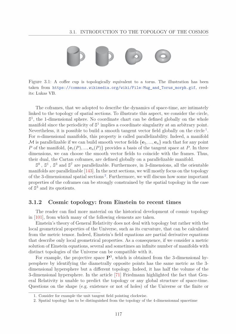
3.1. INTRODUCTION TO THE TOPOLOGY OF THE COSMOS
Figure 3.1: A coffee cup is topologically equivalent to a torus. The illustration has beentaken from https://commons.wikimedia.org/wiki/File:Mug_and_Torus_morph.gif, cred-its: Lukas VB.
The coframes, that we adopted to describe the dynamics of space-time, are intimatelylinked to the topology of spatial sections. To illustrate this aspect, we consider the circle,S
1, the 1-dimensional sphere. No coordinate chart can be defined globally on the wholemanifold since the periodicity of S1 implies a coordinate singularity at an arbitrary point.Nevertheless, it is possible to build a smooth tangent vector field globally on the circle 1.For n-dimensional manifolds, this property is called parallelizability. Indeed, a manifoldM is parallelizable if we can build smooth vector fields {e1, ..., en} such that for any pointP of the manifold, {e1(P ), ..., en(P )} provides a basis of the tangent space at P . In threedimensions, we can choose the smooth vector fields to coincide with the frames. Thus,their dual, the Cartan coframes, are defined globally on a parallelizable manifold.S
0 , S1 , S3 and S7 are parallelizable. Furthermore, in 3-dimensions, all the orientablemanifolds are parallelizable [143]. In the next sections, we will mostly focus on the topologyof the 3-dimensionnal spatial sections 2. Furthermore, we will discuss how some importantproperties of the coframes can be strongly constrained by the spatial topology in the caseof S3 and its quotients.
3.1.2 Cosmic topology: from Einstein to recent timesThe reader can find more material on the historical development of cosmic topology
in [101], from which many of the following elements are taken.Einstein’s theory of General Relativity does not deal with topology but rather with the
local geometrical properties of the Universe, such as its curvature, that can be calculatedfrom the metric tensor. Indeed, Einstein’s field equations are partial derivative equationsthat describe only local geometrical properties. As a consequence, if we consider a metricsolution of Einstein equations, several and sometimes an infinite number of manifolds withdistinct topologies of the Universe can be compatible with it.
For example, the projective space P3, which is obtained from the 3-dimensional hy-persphere by identifying the diametrally opposite points has the same metric as the 3-dimensional hypersphere but a different topology. Indeed, it has half the volume of the3-dimensional hypersphere. In the article [71] Friedmann highlighted the fact that Gen-eral Relativity is unable to predict the topology or any global structure of space-time.Questions on the shape (e.g. existence or not of holes) of the Universe or the finite or
1. Consider for example the unit tangent field pointing clockwise.2. Spatial topology has to be distinguished from the topology of the 4-dimensionnal spacetime
117
CHAPTER 3. TOPOLOGY AND HODGE DECOMPOSITION: A GLOBALAPPROACH TO FIRST-ORDER SOLUTIONS
infinite nature of the Universe could not be adressed by this intrinsically local theory.The modern problem of quantification of gravity shed a new light on the issue of the
topology of space-time, which was mostly ignored until that time. Some constraints ontopology came from the quantification of gravity, as in the case of the quantum gravityscenario of the birth of the Universe (which envolves quantum vacuum fluctuations). Thisscenario is only possible if spacelike hypersurfaces are compact.
Many topologies for the Universe have been considered throughtout time. In 1900,before Einstein invented his theory of General Relativity, Schwarzschild imagined a torustopology of space [133]: “One could imagine that as a result of enormously extendedastronomical experience, the entire universe consists of countless identical copies of ourMilky Way, that the infinite space can be partitioned into cubes each containing an exactlyidentical copy of our Milky Way. Would we really cling on to the assumption of infinitelymany identical repetitions of the same world? . . .We would be much happier with the viewthat these repetitions are illusory, that in reality space has peculiar connection propertiesso that if we leave any one cube through a side, then we immediately reenter it throughthe opposite side”. Nevertheless, when Einstein applied his theory to the Universe, heassumed that space was a positively curved, finite and simply-connected space withoutboundary. Multiconnectedness did not attract much support until lately even if Ellis’ [61]or Zeld’ovich’s [162] work on topology did not exclude it. Allowing multiconnectedness,finite spatial hypersurfaces with zero or negative curvature could exist.
3.1.3 Observational evidence for multiconnected spaces?In this part, I present and discuss some of the signatures of topology in observations.
Recent work by Roukema [114, 127] is aimed at constraining and determining the topologyof the comoving hypersurfaces by observational data. In [127] the author first explains how,in the Newtonian case, a torus topology T 1 = S1 ×R2 can generate a residual accelerationwhich is not predicted by usual Newtonian theory. Indeed, a mass test particle at distancex from a massive object O will be subjected to the gravitational attraction due to O butalso from the one of the two nearest topological images.
These topological effects on the dynamics, usually ignored, are also discussed in therelativistic case, for the compact Schwarzschild-like solution of the Einstein equationsfurther in [127].
As discussed in [72], CMB measurements report a first Doppler peak shifted by a fewpercents towards larger angular scales with respect to the peak predicted by the standardcold dark matter inflationary model, thus favoring a marginally spherical model.
Moreover, considering a multiconnected topology could be the solution for observa-tional issues such as the lack of large angular scale correlations in the CMB. In [126],Roukema, Bulinski, Szaniewska and Gaudin discussed how the multiconnected Poincarédodecahedron topology could explain the missing fluctuation problem in the CMB. Recentmeasures [92, 136] suggest an overall small positive curvature but missing fluctuations inthe CMB. 3 and 5 year WMAP data estimate the chance of this lack of large angular scalecorrelations for the infinite and flat model to be less than 0, 03% [45]. By considering themulticonnected Poincaré dodecahedron 3-manifold, correlations between density pertur-bations should vanish above the length scale of the order of the size of the 3-manifold,
118
3.2. THE HODGE DECOMPOSITION AND THE FIRST–ORDER SOLUTIONS
thus explaining the missing fluctuation in the CMB.
This last part presented some observational evidences supporting a dodecahedrontopology for the spatial hypersurfaces. It was meant to illustrate how topology may havestrong implications on the dynamics of the Universe and why it has to be considered whencosmological observations are interpreted.
3.2 The Hodge decomposition and the first–order so-lutions
The Cartan formalism enables us to define the fields on the physical space instead ofa global background. In the following, we consider that this physical space, i.e. the spa-tial hypersurface, is a closed 3–dimensional manifold. Then, Thurston’s geometrizationconjecture, that we present shortly thereafter, determines which are the possible topolo-gies of this manifold, that may be multiconnected. Hodge theorem will then allow usto decompose the Cartan coframes into an exact, a coexact and a harmonic part. Theexact part can be absorbed into a redefinition of global coordinates and, thus, defines aparametrization of a flat space section, whereas the non-exact and harmonic parts encodethe true geometrical deviations from the background.
3.2.1 Thurston’s geometrization conjectureThurston’s geometrization conjecture, presented in [143], asserts that every closed 3–
dimensional manifolds can be decomposed as a of 3–dimensional manifolds modeled afterthe 8 model geometries listed by Thurston (see also [96]). This conjecture was proved byPerelman in 2003 using Ricci flow with surgery [117] and implies Poincaré’s conjecture.This conjecture asserts that any closed and simply connected 3–dimensional manifolds inhomeomorphic to the hypersphere S3. In Section III.3.2.5, I will consider that the spatialsections are simply connected 3–dimensional manifold. As we will see, in this case, thedimension of the harmonic space of 1–forms vanishes and the Hodge decomposition issimpler.
We now give some mathematical elements that may be useful to understand the Hodgedecomposition. For a very good introduction to differential geometry and Hodge decom-position, the reader can refer to [69], [113] and [9].
3.2.2 Mathematical tools for the Hodge decompositionThe volume form
On a manifold of dimension n, the volume form is defined from a set of orthonormalcoframes {ηi}, i = 1...n as 3:
ε = η1 ∧ ... ∧ ηn . (3.1)
3. We use different notations with respect to [74]. The components of Levi-Civita tensor in a generalbasis are denoted by εν1...νn
whereas the components of the volume form are εν1...νn.
119
CHAPTER 3. TOPOLOGY AND HODGE DECOMPOSITION: A GLOBALAPPROACH TO FIRST-ORDER SOLUTIONS
For general coframes {ηi}, i = 1...n, the volume form becomes:
ε =√
|g| η1 ∧ ... ∧ ηn =√
|g| ε|μ1...μn| ημ1 ∧ ... ∧ ημn . (3.2)
Where |g| is the absolute value of the determinant of the metric tensor and the verticalbars denote that only components with increasing indices are included in the summation.Then,
εμ1...μn =√
|g| εμ1...μn , (3.3)
where εμ1...μn is the n–dimensional Levi-Civita tensor.
The Hodge-dual, the exterior differential and the codifferential operator δ = d∗
A is a p–vector whose contravariant components are obtained by raising the indicesof a p-form α. The dual of the form α in an n-dimensional space is ∗α:
∗ α = 1(n − p)!εν1...νp μ1...μn−pα|ν1...νp|ημ1 ∧ ... ∧ ημn−p . (3.4)
The codifferential operator δ = d∗
The codifferential operator sends p-forms to (p − 1)-forms. We will either considerclosed manifolds or compact manifolds with boundaries such that the forms we consideror their Hodge-dual are zero when restricted to the boundary. Then, on a Riemannianmanifold if βp is a p-form:
d∗βp = (−1)n(p+1)+1 ∗ d ∗ βp , (3.5)
where the exterior differential was defined in I.2.3.1.
Laplace operator on forms
If A is a vector field in Rn with Cartesian coordinates Ai, then ∇2A is the vector fieldwhose components are (∇2A)i = ∑n
j=1(∂2Ai/∂Xj∂Xj). These coordinates are simply theLaplacian of the coordinates of A. In R3,
∇2A = grad divA − curl curlA . (3.6)
This can be written in an intrinsic form if we consider α1 the 1-form associated to A.Then, in R3, this equation is equivalent to
∇2α1 = − (dd∗ + d∗d) α1 . (3.7)
We define the Laplace-de Rham operator ΔdR which is a mapping from p-forms to p-formsby the negative of the preceding:
ΔdR := dd∗ + d∗d = (d + d∗)2 . (3.8)
120
3.2. THE HODGE DECOMPOSITION AND THE FIRST–ORDER SOLUTIONS
Laplacian of a 1-form and Weizenböck formula
The Weizenböck formula gives the expression of the ΔdR applied to a 1–form ha. Ona coordinate basis dX i, we have:
(ΔdR ha
)i
= −(ha‖k
‖k
)i+ ha
k Rki , (3.9)
where ‖ denotes the Lagrangian covariant derivative and Rki is the 3–Ricci curvature
tensor. The first term involves covariant derivatives and the second one takes into accountexplicitly the local geometry.
If we consider the inertial coordinate system of a flat space, the coefficients of ΔdR
reduce to the usual Laplacian operator, and the Riemann curvature vanishes everywhere.Moreover, if we consider the local inertial coordinates on a given point of a manifold,
ΔdR will also reduce to the usual Laplacian operator and the Ricci curvature will vanishlocally.
Bochner’s theorem shows that, if the oriented closed Riemannian manifold M haseverywhere a positive Ricci curvature, then a harmonic 1–form will vanish identically. Wewill show later that this is also the case for any manifold that has an S3 topology.
3.2.3 Hodge theoremHarmonic forms on closed manifolds
Let M be a closed Riemannian n-dimensionnal manifold. We define a global positivedefinite inner product for
(αp, βp) =∫
Mα ∧ ∗β . (3.10)
Since
(Δαp, αp) = (dd∗α + d∗dα, α) = (d∗α, d∗α) + (dα, dα) =‖ d∗α ‖2 + ‖ dα ‖2 ≥ 0 ,(3.11)
thusΔαp = 0 iff d∗α = 0 and dα = 0 . (3.12)
Thus harmonic forms are both closed and coclosed.
Hodge theorem
The vector space of harmonic p-forms:
Hp = {hp / dhp = 0 = d∗hp} (3.13)
is of finite dimension and Poisson’s equation
ΔdR αp = ρp , (3.14)
has a solution αp iff ρp is orthogonal to Hp.
121
CHAPTER 3. TOPOLOGY AND HODGE DECOMPOSITION: A GLOBALAPPROACH TO FIRST-ORDER SOLUTIONS
Consequence: Hodge decomposition
For any p–form γ, we can find a p–form θ such that γ can be decomposed as:
γp = dαp−1 + d∗βp+1 + hp , (3.15)
where αp−1 = d∗θp, d∗βp+1 = dθp and hp is harmonic. If dΛp−1, δΛp+1 and Hp representthe vector space of, respectively, the exterior derivative of (p−1)–forms, the co–differentialof (p+1)–forms and of the harmonic p–forms, all of them forming subspaces of the local co–tangent space of the Riemannian manifold, we can write this decomposition in a symbolicway:
Λp = dΛp−1 + d∗Λp+1 + Hp . (3.16)The decomposition (3.15) is unique:
γp = dαp−1 + d∗βp+1 + hp = dα′p−1 + d∗β′p+1 + h′p . (3.17)
Thendαp−1 − dα′p−1 = 0 ; d∗βp+1 − d∗β′p+1 = 0 ; hp − h′p = 0 . (3.18)
From this we conclude that
αp−1 = α′p−1 + ap−1 / dap−1 = 0 ; (3.19)
βp+1 = β′p+1 + bp+1 / d∗bp+1 = 0 ; (3.20)hp = h′p . (3.21)
3.2.4 Hodge decomposition of the perturbation fieldsHodge decomposition of a 1–form
A 1–form V can be decomposed according to (3.15) as:
V = d α + d∗β + h / ΔdR h = 0 , (3.22)
where α is a scalar, h a 1–form and β = βij dX i ∧ dXj a 2–form. On the Lagrangiancoordinate basis dX i, we get:
Vi dX i =⎛⎝α|i + gij√
|g|
(√|g|glk gjm βkm
)|l
+ hi
⎞⎠dX i / hk Rk
i −(h‖k
‖k
)i
= 0. (3.23)
A 2–form is antisymmetric. In a 3–dimensional space, it has 3 independent coefficients. Itcan thus be generated from a 1−form. We define the 1–form B = Bi dX i such that
βkm dXk ∧ dXm = gul εukm Bl dXk ∧ dXm . (3.24)
Then, we can show thatgij√|g|
(√|g|glk gjm βkm
)|l
= gijεrljBr |l , (3.25)
122
3.2. THE HODGE DECOMPOSITION AND THE FIRST–ORDER SOLUTIONS
where we have used εijk instead of εijk in the definition of Bi in order to get a covariantobject defined on the curved space. The decomposition then becomes:
Vi dX i =(α|i + gij εuljBu | l + hi
)dX i / hk Rk
i −(h‖k
‖k
)i
= 0 . (3.26)
This decomposition is very similar to the Helmoltz-Hodge decomposition, available on flatspace sections, since the first term is the divergence of a scalar potential while the secondone is the generalization of the curl operator to a curved spatial section.
Helmoltz decomposition from the MR of the Hodge decomposition
In the MR , orthonormal Cartan coframes become exact forms. We can thus associateto them some global coordinates x such that ηa = dfa and x = f(X, t). Hodge decompo-sition in flat space in terms of global coordinates gives the Helmholtz decomposition 4:
V = xVi dxi =(
xα ,i + δij εulj xB u , l + xh i
)dxi / xhi
,k,k = 0. (3.27)
This equation (3.27) can also be formulated as a vector identity:
�V = �∇ xα + �∇ × x�B + x�h / Δ x�h = �0. (3.28)
where Δ denotes the simple Laplace operator with respect to Eulerian coordinates. In theLagrangian coordinates, the MR of (3.26) gives:
XV i dX i =(
Xα|i + gij εulj XB u | l + Xh i
)dX i / Xhi
‖k‖k = 0 . (3.29)
The Christoffel symbols that implicitly appear in the Laplace-de Rham equation for Xhi
are non-zero:Γi
kl = 12√
|g|εabcε
imnfa|kl f b
|m f c|n . (3.30)
From the unicity of Hodge decomposition, we conclude that Xα = xα + k where k is aconstant.
3.2.5 Hodge decomposition of Cartan coframes for S3 and quo-tient topologies
From De-Rham and Hurewitz theorem, we can show that the dimension of the har-monic space of 1–forms on a closed oriented manifold is equal to the dimension of the firstfundamental group (also called closed path group) [15] [48] [50]. For simply connectedmanifolds, the dimension of this group is then 0. This is the case of the S3 topology. Theresults of Hodge theorem for S3 can be extended to its quotients 5. Therefore, on S3 there
4. The metric is diag(1, 1, 1) in these global coordinates.5. The quotients spaces M/Γ are built from the universal covering space M (here S3) and the holon-
omy group Γ. For example, the torus T2 is built from the universal covering R2 and the holonomy groupΓ = {a ex + b ey : a, b ∈ Z}: T2 = R2/Γ whereh ex and ey are non-colinear vectors. For a detailedexplanation of quotient spaces and equivalence classes, the reader can refer to Section 2.1.2 of [113].
123
CHAPTER 3. TOPOLOGY AND HODGE DECOMPOSITION: A GLOBALAPPROACH TO FIRST-ORDER SOLUTIONS
exists γa such that the coframes can be decomposed as
ηa = dαa + d∗βa = ΔdR γa , (3.31)
where αa is a scalar, βa a 2–form and γa a 1–form.We now assume we can encode into the first–order perturbation fields the positive
curvature topology. Then, the decomposition
ηa = a(t) (dXa + Pa) , (3.32)
is still available and since the harmonic space of 1–forms is of dimension 0, from (2.45)and (2.48) we conclude that structure coefficients calculated from EPa are constant intime. Since they are initially zero, EPa represents the integrable part of the perturbationfields.
First–order Hodge decomposition of the perturbation 1–form
We consider the Hodge decomposition for the perturbation field Pa and now denoteby αa, βa, Ba the fields that intervene in its decomposition. These fields are first–orderquantities. Keeping only the first order for this equation reads:
P aj = αa
|j + δrj εulr Bau | l . (3.33)
Note that we would have obtained the same expression if Pa was defined on the back-ground space associated to the metric δij. Nevertheless, the space section is not flat sinceP a
j is not in general integrable 6.We lower the non–coordinate index of P a
j with gai which at first–order is equivalentto δai :
Pij = δaiPaj = αi | j + εul
j Biu | l + hij / hij|k
|k = 0 . (3.34)
3.2.6 From SVT to Hodge decompositionWe now know that, for S3 and quotient topologies, EPa encodes the integrable part
of the perturbations. ThusEPa = dαa . (3.35)
As discussed at the end of Section III.2.4.3, it is thus connected to the scalar modes ofthe S-V-T decomposition.
The complementary part, HΠa, is then linked to d∗βa. Furthermore, we can show thatthe Hodge fields αi and Bij are defined through the following Poisson equations from theperturbation fields 7:
Δ0αj = Pij|i , (3.36)
Δ0Bij = εjmrPir |m . (3.37)
6. This would be the case if εulr Bau | l = 0.
7. We have set B mi |m = 0 since this term does not intervene in the decomposition (3.34) and thus has
no physical relevance.
124
3.3. CONCLUSIONS
Equation (3.36) is consistent with the momentum equation expressed in terms of EPa
(2.37) and here becomes trivially satisfied.From (3.34), we know that Bij represents the non-integrable part of the Cartan defor-
mation fields. It thus contains the true deviations to the flat background. We now wantto understand how the propagative part of Bij can be linked to the tensor modes χ
(1)�ij of
the perturbation fields. (3.37) can be rewritten as:
Δ0Bij = εjmrHΠir |m , (3.38)
which implies that the first–order magnetic part is
Hij = Δ0Bij . (3.39)
As we already discussed in Section III.2.4.3, EPa is straightforwardly related to thescalar modes. It is now possible to link the non-exact part of the Hodge decomposition tothe tensor mode of the S-V-T decomposition:
Δ0Bij = 12εj
mrχ(1)�ir |m . (3.40)
3.3 ConclusionsIn this chapter, after a historical introduction to the cosmic topology, we explained
how it could have an impact on the dynamics of the Universe. My work consisted morespecifically in determining how it could have an effect on the first–order solutions thatwere presented in the last chapter. Indeed, the topology of the spatial sections had tobe considered in order to determine the physical content of the first–order solutions EPij
and HΠij. This could not be achieved with a local description of the manifold sincesome elliptic equations had to be solved, thus needing boundary conditions. For spatiallyclosed hypersurfaces, we could solve the elliptic equations and use the powerful Hodgedecomposition.
Furthermore, in the case of closed and simply connected (i.e. S3) topologies for thespatial hypersurfaces, some results on the contribution of EPij and HΠij to the deviationsfrom flatness were obtained. These results can be generalized to the quotients of S3 topolo-gies. To have a deeper insight into the link between the topology and the physical contentof the perturbative solutions, we should now investigate the case of multiconnected spatialtopologies 8, which do not have the same space of harmonic 1–forms. Moreover, we shouldextend our results to the perturbative solutions of higher orders to determine if the EPa
solution will then generate deviations from flatness.
To obtain the first–order results for S3 topologies, we assumed that the topology ofthe zero–order manifold and the one defined by the first–order perturbations could bedifferent. Then, the first one could be flat while the second one could have a sphericaltopology.
8. Hodge decomposition is available also for the 3–torus T3 which has a harmonic space of 1-forms ofdimension 3.
125
CHAPTER 3. TOPOLOGY AND HODGE DECOMPOSITION: A GLOBALAPPROACH TO FIRST-ORDER SOLUTIONS
We should precisely define the mathematical conditions on the metric tensor in orderto determine if it describes a spatial manifold topologically homeomorphic 9 to S3. This canbe achieved by the Ricci-Hamilton flow, which is available on Riemannian manifolds 10.This geometrical flow is a process that deforms the metric in a way formally analogous tothe diffusion of heat, smoothing out its irregularities. The result of this flow would thenbe a constant positive curvature metric.
9. The Gauss-Bonnet theorem that links the average of the curvature to the topology of the manifold(represented by its genus) for even dimensions, gives a trivial identity. This does not allow us to linkgeometry to topology for odd dimensions. Unfortunately, no extension to it was yet found in this case.
10. For an interesting discussion on the Ricci-Hamilton flow and the averaged inhomogeneities in acosmological context, the reader can refer to [31].
126
Conclusion & Outlook
During the three years of my PhD I had the possibility to work on different projectsin the frame of the Intrinsic Lagrangian description. All these projects were focused on abetter description of the formation of large scale structures in an inhomogeneous approach.
In the introductory part of this thesis, I first explained how the modern representationof the Universe historically emerged. Then, I presented how Einstein elaborated Specialand General Relativity in this context. In his theory of General Relativity, he abandonsNewton’s idea of absolute space and time. Moreover, the localization on the manifold hasno longer an absolute physical meaning and is determined by the dynamical elements ofthe theory. Thus, the local inertial reference frames are determined by gravity.
Afterwards, I presented the SMC and the approximations that it implies. The SMCneglects the coupling between the matter content of the Universe and its geometry. Fur-thermore, it decouples the local from the global dynamics describing a hypothetical ab-solute space-time in homogeneous expansion. Nevertheless, the inhomogeneities have tobe taken into account to describe accurately the average dynamics of the Universe.
In the second part of the introduction I explained in the Newtonian case why the La-grangian approach is much more powerful then the Eulerian one. Motivated by the successof the Newtonian Lagrangian approach, we built its relativistic counterpart. The trajec-tory function, which is the coordinate mapping between the Lagrangian and the Euleriancoordinates, is replaced by the Cartan coframes. These coordinate–independent 1–formsenable a relativistic description of the large scale structure formation. In the third part, Idiscussed the consequences of the inhomogeneities on the global dynamics. In particular,I explained how a backreaction term, which contains both a kinematical and a geometri-cal part, arises from the non-commutation of the spatial averaging and the time evolution.
In the second part of the thesis, after a chapter on the decomposition of the Einsteinequations for a 3 + 1 foliation of space-time, I focused on the gravitoelectromagneticanalogy. I first considered the Newtonian case and then the analogy for the electric andmagnetic parts of the Weyl curvature tensor. As was discussed, these fields are solutionsof Maxwell-like equations.
In the Minkowski Restriction, the Cartan coframes become integrable and thus space-time becomes flat. We used the similarities between the gravitoelectric part of the Einsteinequations and the Lagrange-Newton-System and inverted the Minkowski Restriction tobuild from the Newtonian perturbation scheme to order n the corresponding relativisticsolutions.
127
CONCLUSION & PERSPECTIVES
Since Newtonian perturbative solutions do not describe propagative phenomena suchas gravitational waves, their relativistic generalization is also not expected to describethem. The third part of the thesis considered, in the frame of first–order perturbationtheory, the complementary part to the relativistic generalization of the Newtonian per-turbation solutions. To define our perturbation fields, we used differential geometry andmore precisely differential forms. We discussed the difference between this coordinate-independent approach, which intrinsically describes the perturbation fields on the curvedphysical spacetime, with the one adopted in the standard perturbation approach, whichdefines the perturbation fields on a flat background space-time. The Scalar-Vector-Tensordecomposition used in the standard approach, that is available for fields defined on a flatspace section, does no longer work on curved space sections. Therefore, we considered theHodge theory on closed oriented manifolds, that allows a decomposition of differentialforms into exact, coexact and harmonic parts. We applied this decomposition to the per-turbation 1–forms in the case of a simply connected topology: the S3 topology. For thistopology, we determined which part of the solution contributed to the deviations fromflatness. The EPa represents the integrable part of the perturbation fields and thus doesnot contribute to the deviations.
Furthermore, we discussed at first–order the link between the different parts of the solu-tions and the magnetic part of the Weyl tensor, which contains the physics of gravitationalwaves. Nevertheless, before investigating the physical content of EPa and HΠa to upperorders with the Hodge decomposition, the mathematical conditions on the metric to de-scribe a manifold that has a globally closed topology should be first determined. This canbe achieved by the Ricci-Hamilton flow. Indeed, as we have discussed in Section III.3.2.1,a 3–dimensional manifold can be decomposed as a connected sum of 3–dimensional man-ifolds modeled after the 8 model geometries. The Ricci-Hamilton flow is a process that,on each manifold of this connected sum, deforms the metric in a way formally analogousto the diffusion of heat, smoothing out its irregularities. The result of this flow is then aconstant curvature metric.
The intrinsic perturbation scheme could be improved by defining the perturbationfields with respect to the averaged manifold in an iterative way. Nevertheless, to find thisscheme we need first an accurate averaging procedure for tensors. Furthermore, to im-prove our description of structure formation on small scales we should take into accountmore realistic matter models, containing pressure and vorticity. In order to describe ina Lagrangian way a fluid with vorticity, the 3 + 1 description is no longer possible. ALagrangian description will only be possible in the frame of the 1 + 3 threading approach,since the local rest-frames do no longer form global hypersurfaces.
I am very happy that during my PhD I could contribute to current research in largescale structure formation in the frame of inhomogeneous cosmology. The different projectsI had the pleasure to work on will contribute to the evaluation of the backreaction termfor different cosmological systems. Determining the impact of the inhomogeneities on thedynamics of different cosmological systems will be crucial to build the accurate descriptionof relativistic large scale structure formation.
128
List of Figures
1.1 Average binding energy per nucleon . . . . . . . . . . . . . . . . . . . . . . 18
2.1 Representation of the hierarchical dynamics of collapse of a 3–dimensionalfluid element . . . . . . . . . . . . . . . . . . . . . . . . . . . . . . . . . . . 25
2.2 3 + 1 splitting of space-time. . . . . . . . . . . . . . . . . . . . . . . . . . . 352.3 Lagrangian coordinates . . . . . . . . . . . . . . . . . . . . . . . . . . . . . 36
1.1 Normal vector to the hypersurfaces, 4–velocity and tilt vector . . . . . . . 491.2 3 + 1 foliation of space-time . . . . . . . . . . . . . . . . . . . . . . . . . . 50
1.1 Motion of test particles for two linearly polarized states . . . . . . . . . . . 99
3.1 Torus topology of a coffee cup . . . . . . . . . . . . . . . . . . . . . . . . . 117
129
Appendix A
First Results for the LagrangianPerturbation Theory for PerfectFluids in the Strong LagrangianDescription
130
In this chapter, we no longer consider the dust fluid matter model and describe aperfect fluid flow. I here present the first results that I obtained for this matter model,in the Strong Lagrangian description. This work was carried out in order to obtain therelativistic generalization of the results presented in [3], for a Newtonian Lagrangiandescription of a perfect fluid. Indeed, we have shown that the Lagrangian description isthe most relevant when we study nonlinear structure formation in the expanding Universe.The Lagrangian formulation of Einstein equations has already been proposed in [30] fordust cosmologies, explored by H. Asada and M. Kasai in [7] for a dust fluid with vorticityand by H. Asada for a fluid with pressure [8].
We here develop a formalism that will enable us to describe both the radiation domi-nated era in the Early Universe and the collapsing regions with large velocity dispersion.Allowing pressure in the matter model is a step towards a better description of the dy-namics of structure formation.
In this work, we will focus on perfect fluid cosmologies, thus neglecting all irreversiblephenomena. We will assume that there is no vorticity in the fluid flow.
A.1 Perfect fluid thermodynamics in the Strong La-grangian description
A.1.1 Matter modelsThe perfect fluid description that we develop in this chapter enables us to investigate
the dynamics of the Universe in many different situations and epochs. Indeed, a barotropicequation of state can be assumed for either a radiation fluid, which dominates the totalenergy density at early stages of structure formation, or for fundamental scalar fields.
This description is not only relevant for matter models which are supported by thermo-dynamical pressure. A Newtonian insight in the dynamics of collisionless systems indicatesthat a dynamical pressure force arises due to the formation of multi-stream flows whenshell-crossing singularities in the fluid flow develop. The multi-stream force prevents afraction of the fluid to escape from high density regions. As a result, this fraction fallsonto the central region creating an internal hierarchy of caustics, as was explained inSection I.2.1.2. Such a force, which is tightly related to the velocity dispersion, is not ingeneral isotropic. Furthermore, the evolution equations governing the anisotropic stressesinvolve all velocity moments of the distribution function. Yet, in this work, when we willdescribe such a system, we will assume that the multi-stream force acts isotropically.
A.1.2 Thermodynamics of the perfect fluidWe remind that ρ is the positive rest-mass proper density, ε is the energy density and
u = ε/ρ the specific internal energy. The first thermodynamical identity becomes:
du + p dv = T ds (A.1)
where v = 1/ρ and s is the specific entropy.
131
APPENDIX A. LAGRANGIAN PERTURBATION THEORY FOR PERFECTFLUIDS IN THE STRONG LAGRANGIAN DESCRIPTION
An entropy balance equation can be obtained from the conservation equations of thestress-energy tensor:
Sα;α = η(παβ, qξ, T ) , (A.2)
where Sα = ρsuα + qα/T .
We here neglect all irreversible phenomena. Therefore, qα = 0 and παβ = 0. We thenobtain the stress-energy tensor we formerly postulated. Since η(παβ, qα, T ) is then null,the entropy is constant along the flow lines.
We define the specific enthalpy as:
h(s, P ) := u + pv = ε + P
ρ. (A.3)
It can be considered as a thermodynamical potential. Then, ∂h∂s
)P
=: T and ∂h∂p
)s
=: v .Therefore, for an isentropic evolution, since dh/h = dP/(ε + P ):
h(s, p) = h(s, P0) exp(∫ P
P0
dP
ε + P) . (A.4)
A.1.3 Stress-energy tensor conservation and shift vectorThe conservation of rest-mass density gives:
∇α(ρuα) = 0 ⇒ ρ
ρ= −θ , (A.5)
and the stress-energy tensor conservation equation projected along u leads to
ε − ρ
ρ(ε + p) = 0. (A.6)
We can therefore conclude that:dε = h dρ (A.7)
The contracted Bianchi identities result in the conservation of the stress-energy tensor:∇βT αβ = 0. If we combine this equation with expressions (1.18), we derive the followingenergy and momentum conservation laws:
uα∇βT αβ = 0 ⇔ ε + θ(ε + p) = 0 where θ = ∇αuα (A.8)
fμα∇βT αβ = 0 ⇔ uα∇αuμ = −fα
μ ∇α p
ε + p. (A.9)
The stress-energy tensor conservation equation projected on the rest-frames gives theequation of dynamics of the fluid:
uα = −fβα (ln h),β . (A.10)
132
A.2. FIRST-ORDER SCHEME FOR A RADIATION FLUID
For a Lagrangian flux orthogonal foliation such that u = n and β = 0 since V = 0, it ispossible to show from the geometrical relation:
nα∇αnμ = α|μα
, (A.11)
that (A.10) becomes a relation between the lapse α and the pressure gradient [30]. uα isthen equal to nα∇αnν . In the Strong Lagrangian description, (A.10) relates the shift tothe enthalpy state function. Indeed, we can show that (A.10) is equivalent to:
βi + βip
ε + p= − p|i
ε + p(A.12)
which can be expressed as:βi + βi (ln h) = −(ln h)|i . (A.13)
To show this, we remind that in the Strong Lagrangian description, V = 0 and α = γ.Therefore, uμ = (1, 0) and uμ = (−1, βi)
fαμ ∇α p = (∇μ p + uμ∇0 p) ⇒ fα
i ∇α p = p|i + βi p . (A.14)
Furthermore,
hνiu
μ∇μ uν = δνi uμ∇μ uν = uμui,μ − uμuρ
2 (giρ|μ + gμρ|i − giμ|ρ) (A.15)
= βi − 12(α2 + βkβk)|i = βi ,
since ni = 0 and α2 − βkβk = 1 . Thus, since the spatial and time derivative commute inthe Strong Lagrangian description, we integrate (A.12) to obtain:
βi(X, t) = − 1h(X, t)
(∫ t
h(X, t′) dt′)
|i. (A.16)
A.2 First-order scheme in the Strong Lagrangiandescription for a radiation fluid
A.2.1 First–order shift vector for a radiation fluidThe equation of state for a radiation fluid is:
P (ε) = 13ε . (A.17)
The enthalpy expressed in terms of the energy density and the mass density is
h(ε) = h0ε1/4 ; h(ρ) = H0ρ
1/3 , (A.18)
since ρ = 43ε3/4. The shift vector can thus be rewritten as:
βi = ρ−1/3(X, t)(∫ t
tiρ1/3(X, t′)dt′
)|i
. (A.19)
133
APPENDIX A. LAGRANGIAN PERTURBATION THEORY FOR PERFECTFLUIDS IN THE STRONG LAGRANGIAN DESCRIPTION
At first order, the mass density can be expanded as:
ρ = ρHi
a3
(1 − W
4πG− P
). (A.20)
We conclude that βi is a first–order vector that has the following expression:
βi = Ψ|i where Ψ = −a(t)3
(W
4πG
∫ t
ti
dt′
a(t′) +∫ t
ti
P (X, t′)a(t′) dt′
). (A.21)
A.2.2 Zero and first–order Einstein equationsZero–order Einstein equations
At zero–order, the Hamilton constraint equation (1.30) gives:
6H2 = 16πG(0)ε + 2Λ , (A.22)
while the evolution equation for the extrinsic curvature (1.29) reads:
a
a= Λ + 4πG((0)ε − (0)p) − 2H2 . (A.23)
If we insert (A.22) into (A.23), we get the Raychaudhuri equation:
a
a= Λ − 4πG((0)ε + 3 (0)p) . (A.24)
To obtain these equations, we determined the zero–order for the extrinsic curvature(0)Ki
j = −H δij and for the lapse function. Since the shift function is of order 1, the
lapse function is up to first–order equal to 1.We then inserted these quantities into the Einstein equations (1.29), (1.31) and (1.30).
Furthermore, we used the fact that, as in the irrotational dust fluid case, (0)Γrkj = 0 and
(0)R = 0.
Einstein equations to first–order
The first–order term of the extrinsic curvature is:
(1)Kij = 1
2(
(1)βi|j + (1)β
|ij − (1) hikhkj
)= (1)βi
|j − P ij , (A.25)
where we have assumed that there is no vorticity and where we have inserted the metric(2.59). The trace of this first–order term is:
(1)K = β|k
k − P . (A.26)
The Hamilton constraint at first order gives:
H(P − β
|kk
)− 4 πG (1)ε = −
(1)R4 . (A.27)
134
A.2. FIRST-ORDER SCHEME FOR A RADIATION FLUID
The evolution equation for the extrinsic curvature becomes:
(1)Rij +
(P i
j − βi|j)˙+3H
(P i
j − βi|j)−H δi
j
(βk
|k − P)+4πG((1)p−(1)ε)δi
j = 0 . (A.28)
Finally, the momentum constraint equation becomes:(βk |j − P k
j
)|k −
(βk |k − P
)|j = 8πG((1)p + (1)ε)βj . (A.29)
The Raychaudhuri equation at first–order is:(P − βk
|k)˙+ 2H(P − βk
|k) + 4 πG(
(1)ε + 3 (1)p)
= 0 . (A.30)
First–order Einstein equations for a radiation fluid
If we decompose ε and the pressure p to zero and first–order, we get:
(0)ε = ε0ρ
4/3H ia4 and (1)ε = −ε0
4 ρ4/3H i
3 a4 ( W
4πG+ P ) . (A.31)
Equations (A.27), (A.28), (A.29) and (A.30) then become:
H(P − β
|kk
)+ 2
3
(Λ − 3 a
a
)(W
4πG+ P
)= −
(1)R4 ; (A.32)
(1)Rij +
(P i
j − βi|j)˙+ 3H
(P i
j − βi|j)
= (A.33)
H(βk
|k − P)
δij + 4
9
(3 a
a− Λ
)(W
4πG+ P
)δi
j ;(βk |j − P k
j
)|k −
(βk |k − P
)|j = 16
9
(3 a
a− Λ
)(W
4πG+ P
)βj ; (A.34)
(P − βk
|k)˙+ 2H(P − βk
|k) = 43
(Λ − 3 a
a
)(W
4πG+ P
); (A.35)
and
βk|k = Ψ|k |k = − 1
3a(t)
(W|k |k
4πG
∫ t
ti
dt′
a(t′) +∫ t
ti
P (X, t′)|k |k
a(t′) dt′)
. (A.36)
Expressing W from the initial conditions
If we evaluate (A.30) at t = ti, we get the following equation, since βk|k(ti) = 0:
P (ti, X) + 2HP (ti, X) = 83εH iW (X) . (A.37)
It is thus possible, from initial conditions, to build W|k |k.
135
APPENDIX A. LAGRANGIAN PERTURBATION THEORY FOR PERFECTFLUIDS IN THE STRONG LAGRANGIAN DESCRIPTION
First–order trace equations
We combine the previous equations in such a way that no integral over the timeappears. To do so, we formulate the trace equations such that the shift vector will appearwith the scale factor in front of it. Then, the time derivative of a(t) × βi|j gives:
(aβi|j
)˙ = − 1
3a(t)
(W |i|j4πG
+ P |i|j
). (A.38)
The first–order Hamilton equation (A.32) can be written:
a(P − β
|kk
)− 4 πG (1)ε
a2
a= −a2
a
(1)R4 . (A.39)
The time derivative of this equation gives:
P a + P(
a + 16 πG
3 a2aεH i
)+(
16 πG
3 a2aεH i
( 2a3 − a
a2a2
)+ 1
3a(t)Δ0
)(W
4πG+ P
)= (A.40)
(aa2
a2 − 2a
) (1)R4 −
(1)R4
a2
a,
where Δ0 is the Lagrangian Laplacian operator: |k |k. If we now combine the Hamiltonconstraint and the trace of the evolution equation for the extrinsic curvature, we get thefollowing equation:
a 94
(1)R +(a(P − β
|kk
))˙+ 4 πG ((1)p − 4(1)ε) a = 0 . (A.41)
We insert (A.38) into this equation and get:(
P a + 94a(1)R
)˙+ 1
3a(t)Δ0
(W
4πG+ P
)+ 176 πG
9 εH i
(P
a3 − 3a
a4
(W
4πG+ P
))= 0 .
(A.42)
A.3 Concluding remarksThe equation that we obtain for the trace is a wave equation, since it both implies some
spatial and time derivatives. The wave that propagates is a pressure wave. In order to solvethis equation, we can use the fact that the Ricci scalar can be expressed as: R = 1
a2 R(ti),where R(ti) can be determined by the initial data for the comoving perturbation fields(2.6) and (2.7).
136
Bibliography
[1] P. A. R. Ade et al. [Planck Collaboration], “Planck 2013 results. XV. CMB powerspectra and likelihood,” Astron. Astrophys. 571 (2014) A15 [arXiv:1303.5075[astro-ph.CO]]. 20
[2] P. A. R. Ade et al. [Planck Collaboration], “Planck 2015 results. XIII. Cosmo-logical parameters,” [arXiv:1502.01589 [astro-ph.CO]]. 16
[3] S. Adler and T. Buchert, “Lagrangian theory of structure formation inpressure supported cosmological fluids,” Astron. Astrophys. 343 (1999) 317[arXiv:9806320 [astro-ph]]. 131
[4] A. Alles, T. Buchert, F. Al Roumi and A. Wiegand, “Lagrangian theoryof structure formation in relativistic cosmology. III. Gravitoelectric perturba-tion and solution schemes at any order,” Phys. Rev. D 92 (2015) 2, 023512[arXiv:1503.02566 [gr-qc]]. 2, 56, 72, 86, 91, 101, 106, 107
[5] A. Alles: Inhomogeneous Cosmology: an answer to the Dark Matter and DarkEnergy problems? Ph.D. thesis, Université Lyon 1 (2014).
[6] R. L. Arnowitt, S. Deser and C. W. Misner, “The Dynamics of general relativity,”Gen. Rel. Grav. 40 (2008) 1997 [arXiv:0405109 [gr-qc]]. 34, 39
[7] H. Asada and M. Kasai, “Lagrangian description of the fluid flow with vorticityin the relativistic cosmology,” Phys. Rev. D 59 (1999) 123515 [arXiv:9904005[astro-ph]]. 53, 131
[8] H. Asada, “Lagrangian description of fluid flow with pressure in relativistic cos-mology,” Phys. Rev. D 62 (2000) 127301 [arXiv:0010349 [astro-ph]]. 131
[9] T. Aubin, “Some Nonlinear Problems in Riemannian Geometry,” Springer, NewYork (1998) 398 pp. 119
[10] J. M. Bardeen, “Gauge–invariant cosmological perturbations,” Phys. Rev. D,22 (1982). 73
[11] A. Barnes and R. R. Rowlingson, “Irrotational perfect fluids with a purelyelectric Weyl tensor,” Class. Quant. Grav. 6, 949 (1989). 73
137
BIBLIOGRAPHY
[12] J. D. Bekenstein, “Relativistic gravitation theory for the MOND paradigm,”Phys. Rev. D 70 (2004) 083509 [Phys. Rev. D 71 (2005) 069901] [arXiv:0403694[astro-ph]]. 1
[13] F. Bernardeau, S. Colombi, E. Gaztanaga and R. Scoccimarro, “Large scalestructure of the universe and cosmological perturbation theory,” Phys. Rept.367 (2002) 1 [arXiv:0112551 [astro-ph]]. 22, 28
[14] E. Bertschinger and A. J. S. Hamilton, “Lagrangian evolution of the Weyl ten-sor,” Astrophys. J. 435 (1994) 1 [arXiv:9403016 [astro-ph]]. 63, 65, 73
[15] H. Brezis, “Analyse fonctionnelle : Théorie et applications ” Dunod, Paris (2005)ISBN-13 978-2100043149 123
[16] S. Bildhauer, T. Buchert and M. Kasai, “Solutions in Newtonian cosmology –the pancake theory with cosmological constant,” Astron Astrophys. 263, 23(1992). 86
[17] V. R. Bouillot, J. M. Alimi, P. S. Corasaniti and Y. Rasera, “Probing dark en-ergy models with extreme pairwise velocities of galaxy clusters from the DEUS-FUR simulations,” Mon. Not. Roy. Astron. Soc. 450 (2015) 145 [arXiv:1405.6679[astro-ph.CO]]. 27
[18] V. B. Braginsky, C. M. Caves and K. S. Thorne, “Laboratory Experiments toTest Relativistic Gravity,” Phys. Rev. D 15 (1977) 2047.
[19] M. Bruni, S. Matarrese and O. Pantano: “ Dynamics of silent universes,” Astro-phys. J. 445 (1995) 958 [arXiv:9406068[astro-ph.CO]]. 73
[20] T. Buchert and G. Götz, “ A class of solutions for self–gravitating dust in New-tonian gravity,” J. Math. Phys. 28, (1987) 2714.
[21] T. Buchert, “A class of solutions in Newtonian cosmology and the pancake the-ory,” Astron. Astrophys. 223 (1989) 9. 30, 86, 89
[22] T. Buchert, “Lagrangian theory of gravitational instability of Friedmann–Lemaître cosmologies and the ‘Zel’dovich approximation’,” Mon. Not. Roy. Astr.Soc. 254 (1992) 729 . 86, 89
[23] T. Buchert, “Lagrangian perturbation theory – a key–model for large–scale struc-ture,” Astron Astrophys. 267 (1993) L51 . 89
[24] T. Buchert and J. Ehlers, “ Lagrangian theory of gravitational instability ofFriedmann–Lemaître cosmologies – second order approach: an improved modelfor nonlinear clustering,” Mon. Not. Roy. Astron. Soc. 264 (1993) 375 . 86, 90
[25] T. Buchert, “ Lagrangian theory of gravitational instability of Friedmann-Lemaître cosmologies: generic third–order model,” for nonlinear clustering. Mon.Not. Roy. Astron. Soc. 267 (1994) 811 [arXiv:9309055 [astro-ph]].
138
BIBLIOGRAPHY
[26] T. Buchert, “Lagrangian perturbation approach to the formation of largescale structure,” In Varenna 1995, Dark matter in the universe* 543-564[arXiv:9509005 [astro-ph]]. 28, 31
[27] T. Buchert: Lagrangian Perturbation Approach to the Formation of Large–scaleStructure. In Proceedings of the international school of physics Enrico Fermi.Course CXXXII: Dark matter in the Universe, edited by S. Bonometto, J. Pri-mack and A. Provenzale (Società Italiana di Fisica, Varenna sul Lago di Como,1996). 31
[28] T. Buchert and J. Ehlers, “ Averaging inhomogeneous Newtonian cosmologies,”Astron. Astrophys. 320 (1997) 1. [arXiv:9510056 [astro-ph]]. 80
[29] T. Buchert, “On average properties of inhomogeneous fluids in general relativity.1. Dust cosmologies,” Gen. Rel. Grav. 32 (2000) 105 [arXiv:9906015 [gr-qc]]. 2,41
[30] T. Buchert, “On average properties of inhomogeneous fluids in general relativity:Perfect fluid cosmologies,” Gen. Rel. Grav. 33 (2001) 1381 [arXiv:0102049 [gr-qc]]. 2, 131, 133
[31] T. Buchert and M. Carfora, “Regional averaging and scaling in relativistic cos-mology,” Class. Quant. Grav. 19 (2002) 6109 [arXiv:0210037 [gr-qc]]. 126
[32] T. Buchert and A. Dominguez, “Adhesive gravitational clustering,” Astron. As-trophys. 438 (2005) 443 [arXiv:0502318 [astro-ph]]. 28
[33] T. Buchert, “An Exact Lagrangian integral for the Newtonian gravitational fieldstrength,” Phys. Lett. A 354 (2006) 8 [arXiv:0508059 [gr-qc]]. 58
[34] T. Buchert, “ Toward physical cosmology: focus on inhomogeneous geome-try and its nonperturbative effects,” Class. Quant. Grav. 28 (2011) 164007.[arXiv:1103.2016 [gr-qc]] 43
[35] T. Buchert and M. Ostermann, “Lagrangian theory of structure formation in rel-ativistic cosmology I: Lagrangian framework and definition of a non-perturbativeapproximation,” Phys. Rev. D 86 (2012) 023520 [arXiv:1203.6263 [gr-qc]]. 2, 31,55, 66, 73, 74, 77, 88
[36] T. Buchert, C. Nayet and A. Wiegand, “Lagrangian theory of structure forma-tion in relativistic cosmology II: average properties of a generic evolution model,”Phys. Rev. D 87 (2013) 12, 123503 [arXiv:1303.6193 [gr-qc]]. 2, 55, 73
[37] T. Buchert, “Introduction to Gravitation Theories, 2013 Master 1 ENS Lyonlecture notes”
[38] T. Buchert, “Cosmology and Gravitational Systems, 2013 Master 2 ENS Lyonlecture notes” 22, 28, 58
139
BIBLIOGRAPHY
[39] M. N. Celerier, K. Bolejko and A. Krasinski, “A (giant) void is not mandatory toexplain away dark energy with a Lemaitre – Tolman model,” Astron. Astrophys.518 (2010) A21 [arXiv:0906.0905 [astro-ph.CO]].
[40] S. Chandrasekhar, “The Mathematical Theory of Black Holes,” Oxford Univer-sity Press (1998) ISBN 978-0198503705 75
[41] S. Nadkarni–Ghosh and D. F. Chernoff, “ Extending the domain of validity ofthe Lagrangian approximation,” Mon. Not. Roy. Astron. Soc. 410, (2011) 1454[arXiv:1005.1217 [gr-qc]].
[42] S. Nadkarni–Ghosh and D. F. Chernoff, “ Modelling non–linear evolution usingLagrangian perturbation theory re–expansions,” Mon. Not. Roy. Astron. Soc.431 (2013) 799 [arXiv:1211.5777 [gr-qc]].
[43] C. Clarkson, G. Ellis, J. Larena and O. Umeh, “Does the growth of struc-ture affect our dynamical models of the universe? The averaging, backreac-tion and fitting problems in cosmology,” Rept. Prog. Phys. 74 (2011) 112901[arXiv:1109.2314 [astro-ph.CO]]. 40, 43
[44] A. Conley et al. [SNLS Collaboration], “Supernova Constraints and SystematicUncertainties from the First 3 Years of the Supernova Legacy Survey,” Astro-phys. J. Suppl. 192 (2011) 1 [arXiv:1104.1443 [astro-ph.CO]].
[45] C. J. Copi, D. Huterer, D. J. Schwarz and G. D. Starkman, “No large-anglecorrelations on the non-Galactic microwave sky,” Mon. Not. Roy. Astron. Soc.399 (2009) 295 [arXiv:0808.3767 [astro-ph]]. 118
[46] L. F. O. Costa and J. Natario, “Gravito-electromagnetic analogies,” Gen. Rel.Grav. 46 (2014) 1792 [arXiv:1207.0465 [gr-qc]]. 58
[47] R. Cowen, “ Full-Galaxy dust map muddles search for gravitational waves,”Nature news, Sep. 22, (2014) 96
[48] G. De Rham, “ Sur la théorie des formes différentielles harmoniques ,” Annalesde l’Universite de Grenoble 22 (1946) 135-152 123
[49] R. H. Dicke, P. J. E. Peebles, P. G. Roll and D. T. Wilkinson, “Cosmic Black-Body Radiation,” Astrophys. J. 142 (1965) 41 19
[50] J. Dieudonné, “ Eléments d’analyse réelle ,” Tome 1 22 (1966) 123
[51] R. Durrer, “ Gauge invariant cosmological perturbation theory ,” Fund. CosmicPhys. 15 (1994) 209. [arXiv:9311041 [astro-ph]]. 73
[52] J. S. Dowker, “A gravitational Aharonov-Bohm effect,” Il Nuovo Cimento BSeries 10 52 (1967) 129-135 57
140
BIBLIOGRAPHY
[53] J. Ehlers, “Contributions to the relativistic mechanics of continuous media,”Gen. Rel. Grav. 25 (1993) 1225 [Abh. Akad. Wiss. Lit. Mainz. Nat. Kl. 11(1961) 793].
[54] J. Ehlers, “Examples of Newtonian limits of relativistic spacetimes,” Class.Quant. Grav. 14 (1997) 119
[55] J. Ehlers and T. Buchert, “Newtonian cosmology in Lagrangian formula-tion: foundations and perturbation theory,” Gen. Rel. Grav. 29 (1997) 733[arXiv:9609036 [astro-ph]]. 31, 75, 76, 77, 78, 79, 80, 81, 83
[56] J. Ehlers, I. Ozsvath, E. L. Schücking and Y. Shang, “Pressure as a source ofgravity,” Phys. Rev. D 72 (2005) 124003 [arXiv:0510041 [gr-qc]]. 61
[57] J. Ehlers, I. Ozsvath and E. L. Schucking, “Active mass under pressure,” Am.J. Phys. 74 (2006) 607 [arXiv:0505040 [gr-qc]].
[58] J. Ehlers and T. Buchert, “On the Newtonian Limit of the Weyl Tensor,” Gen.Rel. Grav. 41 (2009) 2153 [arXiv:0907.2645 [gr-qc]]. 65
[59] A. Einstein, “Die Grundlage der allgemeinen Relativitatstheorie,” Ann. Phys.49 (1916) 769-822 11
[60] A. Einstein, “ Über Gravitationswellen,” Preussische Akamedie der Wis-senschaften, Sitzungsberichte, (1918), 154. 96
[61] G. F. R. Ellis, “Topology and cosmology,” Gen. Rel. Grav. 2 (1971) 7. 118
[62] G. F. R. Ellis, M. Bruni, “ Covariant and gauge–invariant approach to cosmo-logical density fluctuations,” Phys. Rev. D 40 (1989) 1804. 73
[63] G. F. R. Ellis, J. Hwang, M. Bruni: Covariant and gauge–independent perfectfluid Robertson–Walker perturbations,” Phys. Rev. D 40 (1989) 1819. 73
[64] G. F. R. Ellis and H. van Elst, “Cosmological models: Cargese lectures 1998,”NATO Sci. Ser. C 541 (1999) 1 [arXiv:9812046]. 62
[65] G. F. R. Ellis, “Inhomogeneity effects in Cosmology,” Class. Quant. Grav. 28(2011) 164001 [arXiv:1103.2335 [astro-ph.CO]]. 39, 40, 43
[66] H. van Elst, C. Uggla, W. M. Lesame, G. F. R. Ellis and R. Maartens:,“Integrability of irrotational silent cosmological models,” Class. Quant. Grav.14 (1997) 1151 [arXiv:9611002 [gr-qc]]. 73
[67] H. van Elst and G. F. R. Ellis, “The Covariant approach to LRS perfect fluidspace-time geometries,” Class. Quant. Grav. 13 (1996) 1099 [arXiv:9510044 [gr-qc]]. 40
[68] H. van Elst and C. Uggla, “General relativistic (1+3) orthonormal frame ap-proach revisited,” Class. Quant. Grav. 14 (1997) 2673 [arXiv:9603026 [gr-qc]].54
141
BIBLIOGRAPHY
[69] T. Frankel, “The geometry of physics: An introduction,” Cambridge, UK: Univ.Pr. (1997) 654 p 119
[70] A. Friedmann, “Über die Krummung des Raumes,” Zeits. Phys. 10, (1922), 377-386 13
[71] A. Friedmann, “ The Universe as Space and Time” Petrograd, Akademiya (1923)117
[72] E. Gausmann, R. Lehoucq, J. P. Luminet, J. P. Uzan and J. Weeks, “Topologicallensing in spherical spaces,” Class. Quant. Grav. 18 (2001) 5155 [arXiv:0106033[gr-qc]]. 116, 118
[73] E. Gourgoulhon, “3+1 formalism and bases of numerical relativity,”[arXiv:0703035 [gr-qc]]. 34, 35, 49, 53, 96
[74] O. Gron, and H. Sigbjorn, “ Einstein’s General Theory of Relativity,” Springer,New York (2007) ISBN 978-0-387-692005 9, 32, 62, 75, 96, 99, 119
[75] A.Hamilton : General Relativity, Black Holes, and Cosmology. http://jila.colorado.edu/~ajsh/astr5770_14/grbook.pdf, (2014). 19, 32
[76] O. Heaviside, “ A Gravitational and Electromagnetic Analogy,” Part I, TheElectrician, 31, (1893), 281-282. 57, 61
[77] C. Hikage, J. Schmalzing, T. Buchert, Y. Suto, I. Kayo, A. Taruya, M. S. Vogeley,F. Hoyle, J. R. Gott, III, and J. Brinkmann, “ Minkowski Functionals of SDSSGalaxies I : Analysis of Excursion Sets,” Publications of the Astronomical Societyof Japan, 55, (2003), 911-931 [arXiv:astro-ph/0304455]. 12
[78] G. Holzmüller, “ Minkowski Functionals of SDSS Galaxies I : Analysis of Excur-sion Sets,” Z. Math. Phys. , 15, (1870), 69. 57
[79] F. Hoyle, Fiona, M.Vogeley, “ Voids in the Point Source Catalogue Survey andthe Updated Zwicky Catalog,” The Astrophysical Journal, 566, 1 (2002), 641-651 [arXiv:astro-ph/0109357]. 38
[80] F. Hoyle, Fiona, M.Vogeley, “ Voids in the Two-Degree Field Galaxy RedshiftSurvey,” The Astrophysical Journal, 607, 1 (2004), 751-764. 38
[81] E. P. Hubble, “ Cepheids in Spiral Nebulae,” Popular Astronomy, 33 (1925),252. 8
[82] E. P. Hubble, “ NGC 6822, a remote stellar system,” Astrophysical Journal, 62(1925), 409-433. 8
[83] X. Jaen and A. Molina, “Rigid motions and generalized Newtonian gravitation,”Gen. Rel. Grav. 45 (2013) 1531 [arXiv:1210.1137 [gr-qc]].
142
BIBLIOGRAPHY
[84] R. Jantzen, P. Carini, D. Bini, “ GEM: The User Manual–Understanding Space-time Splittings and their Relationships,” URL:www.homepage.villanova.edu/robert.jantzen/gem, (2004). 58
[85] M. Kasai, “Tetrad-based perturbative approach to inhomogeneous universes: Ageneral relativistic version of the Zel’dovich approximation,” Phys. Rev. D 52(1995) 5605. 31, 73
[86] R. P. Kerr, “Gravitational field of a spinning mass as an example of algebraicallyspecial metrics,” Phys. Rev. Lett. 11 (1963), 237-238. 11
[87] M. Kerscher, K. Mecke, J. Schmalzing, C. Beisbart, T. Buchert, and H. Wag-ner, “ Morphological fluctuations of large-scale structure: The PSCz survey,”Astronomy and Astrophysics, 373, (2001), 1-11 [arXiv:0101238 [astro-ph]]. 12
[88] H. Kodama and M. Sasaki, “ Cosmological Perturbation Theory,” Progress ofTheoretical Physics Supplement 78 (1984) 1. 73
[89] L. Kofman and D. Pogosian, “Equations of gravitational instability are nonlo-cal,” Astrophys. J. 442 (1995) 30 [arXiv:9403029 [astro-ph]]. 65, 73
[90] E. W. Kolb and M. S. Turner, “The Early universe,” Front. Phys. 69 (1990) 1.11
[91] E. W. Kolb, “Backreaction of inhomogeneities can mimic dark energy,” Class.Quant. Grav. 28 (2011) 164009. 43
[92] E. Komatsu et al. [WMAP Collaboration], “Five-Year Wilkinson MicrowaveAnisotropy Probe (WMAP) Observations: Cosmological Interpretation,” Astro-phys. J. Suppl. 180 (2009) 330 [arXiv:0803.0547 [astro-ph]]. 118
[93] S. M. Kopeikin, A. N. Petrov, “ Dynamic field theory and equations of motionin cosmology,” Ann. of Phys. 350 (2014) 379 [arXiv:1407.3846 [gr-qc]].
[94] M. Kuhlen, M. Vogelsberger, R.. Angulo, “Numerical simulations of the darkuniverse: State of the art and the next decade,” Physics of the Dark Universe,1 (2012) 50 [arXiv:1209.5745 [astro-ph]]. 28
[95] F. S. Labini, “Inhomogeneities in the universe,” Class. Quant. Grav. 28 (2011)164003 [arXiv:1103.5974 [astro-ph.CO]]. 12
[96] M. Lachieze-Rey and J. P. Luminet, “Cosmic topology,” Phys. Rept. 254 (1995)135 [arXiv:9605010 [gr-qc]]. 119
[97] G. Lemaitre, “Un univers homogene de masse constante et de rayon croissant,rendant compte de la vitesse radiale des nebuleuses extra-galactiques,” Ann. Soc.Sci. Bruxelles A 46, (1927), 49-59. 13
[98] J. Lesgourgues, “Cosmology, ENS Lyon lecture notes’,’ available on"http://lesgourg.web.cern.ch/lesgourg/courses.html" 11, 16
143
BIBLIOGRAPHY
[99] N. Li and D.J. Schwarz: On the onset of cosmological backreaction. Phys. Rev.D 76, 083011 (2007) [arXiv:0702043 [gr-qc]]. 91
[100] J. P. Luminet and B. F. Roukema, “Topology of the universe: Theory and ob-servation,” [arXiv:9901364].
[101] J. P. Luminet, “Past and future of cosmic topology,” Acta Cosmologica 24 (1998)105 [arXiv:9804006 [gr-qc]]. 117
[102] R. Maartens, G. F. R. Ellis and W. R. Stoeger, S.J., “Limits on anisotropy andinhomogeneity from the cosmic background radiation,” Phys. Rev. D 51 (1995)1525 [arXiv:9501016 [astro-ph]]. 1, 39
[103] R. Maartens, G. F. R. Ellis and W. R. Stoeger, S.J., “Anisotropy and inhomo-geneity of the universe from Delta(T) / T,” Astron. Astrophys. 309 (1996) L7[arXiv:9510126 [astro-ph]]. 1, 39
[104] B. Mashhoon, F. W. Hehl and D. S. Theiss, “On the Gravitational effects ofrotating masses - The Thirring-Lense Papers,” Gen. Rel. Grav. 16 (1984) 711.57
[105] S. Matarrese, O. Pantano and D. Saez, “ General relativistic dynamics of ir-rotational dust: Cosmological implications,” Physical Review Letters (1994) 72320–323 [arXiv:9310036 [astro-ph]]. 73
[106] S. Matarrese, O. Pantano and D. Saez, “ A relativistic approach to gravita-tional instability in the expanding Universe – Second–order Lagrangian so-lutions,” Monthly Notices of the Royal Astronomical Society (1994) 271513[arXiv:9403032 [astro-ph]]. 73
[107] S. Matarrese, S. Mollerach, and M. Bruni, “ Relativistic second–order perturba-tions of the Einstein–de Sitter Universe,” Phys. Rev. D 58 (1998) [arXiv:9707278[astro-ph]]. 73, 111, 112
[108] A. L. Melott, B. S. Sathyaprakash and V. Sahni, “Evolution of the poten-tial in cosmological gravitational clustering,” Astrophys. J. 456 (1996) 65[arXiv:9504087 [astro-ph]]. 31
[109] A. L. Melott, T. Buchert and A. G. Weiss, “Testing higher order Lagrangian per-turbation theory against numerical simulations. 2: Hierarchical models,” Astron.Astrophys. 294 (1995) 345 [arXiv:9404018 [astro-ph]]. 31
[110] A.A. Michelson and E.W. Morley, “On the Relative Motion of the Earth and theLuminiferous Ether,” Philos. Mag. S 5 24 (1887) 151 [arXiv:1108.0548 [hep-ph]].9
[111] M. Milgrom, “A Modification of the Newtonian dynamics as a possible alterna-tive to the hidden mass hypothesis,” Astrophys. J. 270 (1983) 365. 1
144
BIBLIOGRAPHY
[112] V. F. Mukhanov, H. A. Feldman, and R. H. Brandenberger, “ Theory ofcosmological perturbations,” Phys. Rep. 215 (1992) 203. 73
[113] M. Nakahara, “Geometry, topology and physics,” Boca Raton, USA: Taylor andFrancis (2003) 573 p 119, 123
[114] J. J. Ostrowski, B. F. Roukema and Z. P. Bulinski, “A relativistic modelof the topological acceleration effect,” Class. Quant. Grav. 29 (2012) 165006[arXiv:1109.1596 [astro-ph.CO]]. 116, 118
[115] P. Peebles, “Large-Scale Structure of the Universe ” Princeton University Press(1980) 440 p 27
[116] A. A. Penzias and R. W. Wilson, “A Measurement of excess antenna temperatureat 4080-Mc/s,” Astrophys. J. 142 (1965) 419. 19
[117] G. Perelman, “The Entropy formula for the Ricci flow and its geometric appli-cations,” [math/0211159 [math-dg]]. 119
[118] S. Perlmutter et al. [Supernova Cosmology Project Collaboration], “Measure-ments of Omega and Lambda from 42 high redshift supernovae,” Astrophys. J.517 (1999) 565 [arXiv:9812133[astro-ph]]. 13
[119] A. D. Polyanin and V. F. Zaitsev, “Handbook of exact solutions for ordinarydifferential equations,” Boca Raton: CRC Press (1995). 84
[120] C. Rampf and T. Buchert, “Lagrangian perturbations and the matter bispec-trum I: fourth–order model for nonlinear clustering,” J. C. A. P. 06 (2012) 021[arXiv:1203.4260[gr-qc]]. 74
[121] C. Rampf and Y. Y. Y. Wong, “ Lagrangian perturbations and the matterbispectrum II: the resummed one–loop correction to the matter bispectrum,” J.C. A. P. 06 (2012) 018 [arXiv:1203.4261[gr-qc]]. 74
[122] C. Rampf and G. Rigopoulos, “ Zel’dovich approximation and general relativity,”Mon. Not. Roy. Astron. Soc. 430 (2013) L54 [arXiv:1210.5446[gr-qc]]. 73
[123] S. Räsänen, “Backreaction: directions of progress,” Class. Quant. Grav. 28(2011) 164008 [arXiv:1102.0408 [astro-ph.CO]]. 43
[124] A. G. Riess et al. [Supernova Search Team Collaboration], “Observational evi-dence from supernovae for an accelerating universe and a cosmological constant,”Astron. J. 116 (1998) 1009 [arXiv:9805201 [astro-ph]]. 13
[125] H. Robertson, “On the foundations of relativistic cosmology,” Proc. Natl. Acad.Sci. USA 15, (1929), 822-829. 13
[126] B. F. Roukema, Z. Bulinski, A. Szaniewska and N. E. Gaudin, “The optimalphase of the generalised Poincare Dodecahedral Space hypothesis implied by thespatial cross-correlation function of the WMAP sky maps,” Astron. Astrophys.486 (2008) 1, 55 [arXiv:0801.0006 [astro-ph]]. 116, 118
145
BIBLIOGRAPHY
[127] B. F. Roukema, "Cosmic topology affects dynamics", Acta Physica Polonica B42 (2011) 2273 [arXiv:1201.0971 [astro-ph.CO]]. 116, 118
[128] B. F. Roukema, T. Buchert, H. Fujii and J. J. Ostrowski, “Is the baryon acous-tic oscillation peak a cosmological standard ruler?” [arXiv:1506.05478 [astro-ph.CO]]. 12
[129] X. Roy, T. Buchert, “On Average Properties of Inhomogeneous Fluids in GeneralRelativity III: General Foliations, ” in preparation. 48
[130] C. Rovelli, “Quantum Gravity ” Cambridge University Press (2007) 488 p 9, 10,32, 33
[131] H. Russ, M. Morita, M. Kasai and G. Börner, “ Zel’dovich–type approximationfor an inhomogeneous universe in general relativity: second–order solutions,”Phys. Rev. D 53 (1996) 6881. [arXiv:9512071 [astro-ph]]. 73
[132] D. S. Salopek, J. M. Stewart and K. M. Croudace, “ The Zel’dovich Approxi-mation and the relativistic Hamilton–Jacobi Equation,” Mon. Not. Roy. Astron.Soc. 271 (1994) 1005 [arXiv:9403053 [astro-ph]]. 73
[133] K. Schwarzschild, Vierteljahrschrift der Ast. Ges. 35 (1900) 67 118
[134] K. Schwarzschild, “Uber das Gravitationsfeld eines Massenpunktes nach der Ein-stein’schen Theorie” Sitzungsber. Preuss. Akad. Wiss. 7 (1916), 189-196. 11
[135] L. Smarr and J. W. York, Jr., “Kinematical conditions in the construction ofspace-time,” Phys. Rev. D 17 (1978) 2529. 49, 53
[136] D. N. Spergel et al. [WMAP Collaboration], “Wilkinson Microwave AnisotropyProbe (WMAP) three year results: implications for cosmology,” Astrophys. J.Suppl. 170 (2007) 377 [arXiv:0603449 [astro-ph]]. 118
[137] V. Springel, “The Cosmological simulation code GADGET-2,” Mon. Not. Roy.Astron. Soc. 364 (2005) 1105 [arXiv:0505010 [astro-ph]]. 28
[138] N. Straumann, “ General Relativity with Applications in Astrophysics,”Springer Verlag (2004) ISBN 978-3-642-06013-7 99
[139] R. A. Sussman, “Back-reaction and effective acceleration in generic LTBdust models,” Class. Quant. Grav. 28 (2011) 235002 doi:10.1088/0264-9381/28/23/235002 [arXiv:1102.2663 [gr-qc]]. 43
[140] R. Teyssier, “Cosmological hydrodynamics with adaptive mesh refinement: anew high resolution code called ramses,” Astron. Astrophys. 385 (2002) 337[arXiv:0111367 [astro-ph]]. 28
[141] F. Tisserand, “Cosmological hydrodynamics with adaptive mesh refinement:a new high resolution code called ramses,” Compt. Rend. 75 (1872) 760[arXiv:0111367 [astro-ph]]. 57
146
BIBLIOGRAPHY
[142] R. Thieberger and M.-N. Célérier, “ Scaling Regimes as obtained from the DR5Sloan Digital Sky Survey,” Classical and Quantum Gravity, 28:164003 (2011)[arXiv:0802.0464 [astro-ph]]. 12
[143] W. Thurston, “The Geometry and Topology of Three-Manifolds ” PrincetonUniversity Press (1997) 402 p 117, 119
[144] R. C. Tolman, “Relativity, Thermodynamics and Cosmology ” Oxford, Claren-don Press (1934) 528 p 61
[145] R. C. Tolman, “Effect of Inhomogeneity on Cosmological Models,” Proceedingsof the National Academy of Science, 20 (1934), 169-176. 11
[146] K. Tomita, “Non–linear theory of gravitational instability in the expanding Uni-verse,” Prog. Theor. Phys. 37 (1967) 831 . 73
[147] K. Tomita, “Non–linear theory of gravitational instability in the expanding Uni-verse. II. ,” Prog. Theor. Phys. 45 (1971) 1747. 73
[148] K. Tomita, “Non–linear theory of gravitational instability in the expanding Uni-verse . III.,” Prog. Theor. Phys. 47 (1972) 416. 73
[149] R. Brent Tully, E. J. Shaya, I. D. Karachentsev; H. Courtois, D. Kocevski,L. Rizzi, A. Peel, “ Our Peculiar Motion Away from the Local Void,” The As-trophysical Journal, 676, 1 (2008), 184-205 [arXiv:0705.4139 [astro-ph]].
[150] A. Walker, On Milne’s theory of world-structure, P. Lond. Math. Soc. 42, (1936),90-126. 3813
[151] S. Weinberg, “Gravitation and Cosmology: principles and applications of thegeneral theory of relativity, ” Jhon Wiley and Sons, Inc. (1972) 657 p 11
[152] S. Weinberg, “Cosmology,” Oxford, UK: Oxford Univ. Pr. (2008) 593 p 96, 99
[153] A. G. Weiss, S. Gottlöber and T. Buchert, “Optimizing higher order Lagrangianperturbation theory for cold dark matter models,” Mon. Not. Roy. Astron. Soc.278, 4 (1996), 953-964 [arXiv:9512106 [astro-ph]]. 31
[154] A. Wiegand and T. Buchert, “Multi-scale cosmology and structure-emergingDark Energy: a plausibility analysis,” Phys. Rev. D 82 (2010) 023523[arXiv:1002.3912 [astro-ph.CO]]. 43
[155] A. Wiegand and T. Buchert, “Multiscale approach to inhomogeneous cosmolo-gies,” J. Cosmol. 15 (2011) 6100 [arXiv:1103.1531 [astro-ph.CO]]. 2
[156] A. Wiegand, T. Buchert and M. Ostermann, “Direct Minkowski Functional anal-ysis of large redshift surveys: a new high–speed code tested on the luminous redgalaxy Sloan Digital Sky Survey-DR7 catalogue,” Mon. Not. Roy. Astron. Soc.443 (2014) 1, 241 [arXiv:1311.3661 [astro-ph.CO]]. 12
147
BIBLIOGRAPHY
[157] I. Ciufolini, J.A. Wheeler, “Gravitation and Inertia” Princeton Series in Physics(1995) 512 p 58
[158] D. L. Wiltshire, “What is dust? - Physical foundations of the averaging problemin cosmology,” Class. Quant. Grav. 28 (2011) 164006 [arXiv:1106.1693 [gr-qc]].40, 43
[159] J. Yadav, S. Bharadwaj, B. Pandey, and T. Seshadri, “Testing homogeneity onlarge scales in the Sloan Digital Sky Survey Data Release One,” Mon. Not. Roy.Astron. Soc. 364 (2005), 601-606. [arXiv:0504315 [astro-ph]]. 12
[160] R. M. Zalaletdinov, “Averaging problem in general relativity, macroscopic gravityand using Einstein’s equations in cosmology,” Bull. Astron. Soc. India 25 (1997)401 [arXiv:9703016 [gr-qc]]. 40
[161] Y. B. Zeldovich, “Gravitational instability: An Approximate theory for largedensity perturbations,” Astron. Astrophys. 5 (1970) 84. 2, 30, 73
[162] I. B. Zel’dovich and L. Grishchuk, “Structure and future of the ’new’ universe,”Mon. Not. Roy. Astron. Soc. , 15 (1984) 207 118
148


![Lattice Topological Field Theory in Two Dimensionsmueger/TQFT/FHK.pdfLattice Topological Field Theory in Two Dimensions 159 continuum approach [7]. In Sect. 6, we also study the perturbation](https://img.pdfslide.tips/doc/110x75/5e6d72380c477844e178570f/lattice-topological-field-theory-in-two-muegertqftfhkpdf-lattice-topological.jpg)