Embed Size (px)
Citation preview

Optical Flow and Object Tracking
簡韶逸 Shao-Yi Chien
Department of Electrical Engineering
National Taiwan University
Fall 2018
1

Slide Credits
• Lucas-Kanade algorithm from Prof. Yung-Yu Chuang’s VFX course
• Feature tracker and optical flow from Prof. Jia-Bin Huang’s Computer Vision
• Visual Tracking from Prof. Alexandre Alahi, Stanford Vision Lab
• Slides from members of Media IC and System Lab
2

Outline
• Optical flow• Introduction
• Lucas-Kanade algorithm
• State-of-the-art optical flow• Epicflow
• Flownet
3

Introduction to Optical Flow
• Motion vector for each pixel
• Developed for 3-D motion estimation in the computer vision community
• Optical flow is caused by movement of intensity patterns in an image plane
• Optical flow is what we can only get from video frames
4

Introduction to Optical Flow
5

Introduction to Optical Flow
• Aperture problem
• Ill-pose inverse problem• Not well posed
• Existance: No. Ex. rotating uniform sphere
• Uniquness: No. Aperture problem
• Continuity: No. Sensitive to noise
6

Aperture Problem
7

Aperture Problem
8

Aperture Problem
9

Basic Assumption for Optical Flow
• Brightness consistency
• Spatial coherence
• Temporal persistence
10

11
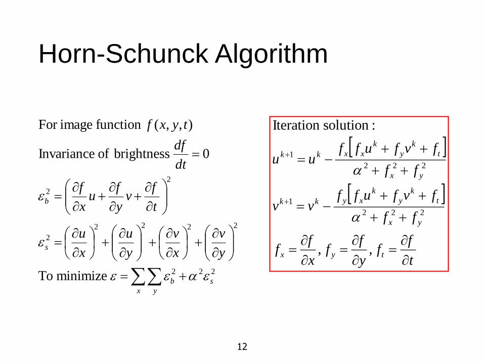
Horn-Schunck Algorithm
• B. K. P. Horn and B. G. Schunck, “Determining optical flow,” Artificial Intelligence, vol. 17, pp. 185—203, 1981.
2222
minimize to:constraint Smoothness
,
0
0 brightness of Invariance
),,(function imageFor
y
v
x
v
y
u
x
u
t
yv
t
xu
t
fv
y
fu
x
f
dt
df
tyxf
12
Horn-Schunck Algorithm
x y
sb
s
b
y
v
x
v
y
u
x
u
t
fv
y
fu
x
f
dt
df
tyxf
222
2222
2
2
2
minimize To
0 brightness of Invariance
),,(function imageFor
t
ff
y
ff
x
ff
ff
fvfuffvv
ff
fvfuffuu
tyx
yx
t
k
y
k
xykk
yx
t
k
y
k
xxkk
,,
:solutionIteration
222
1
222
1

13
Horn-Schunck Algorithm
14
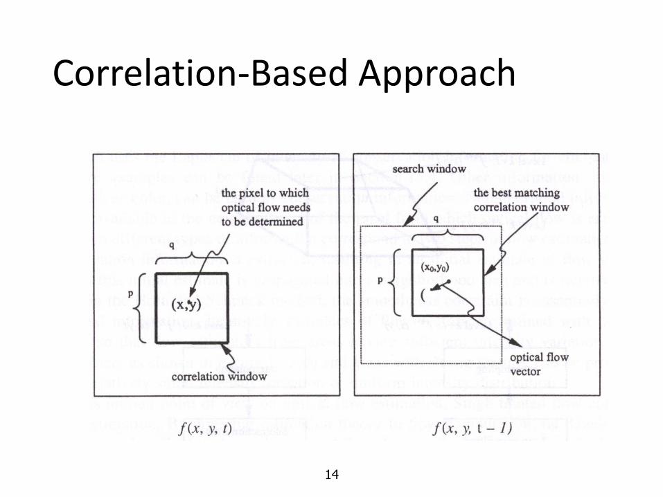
Correlation-Based Approach

15
Some Example
Needle diagram
16
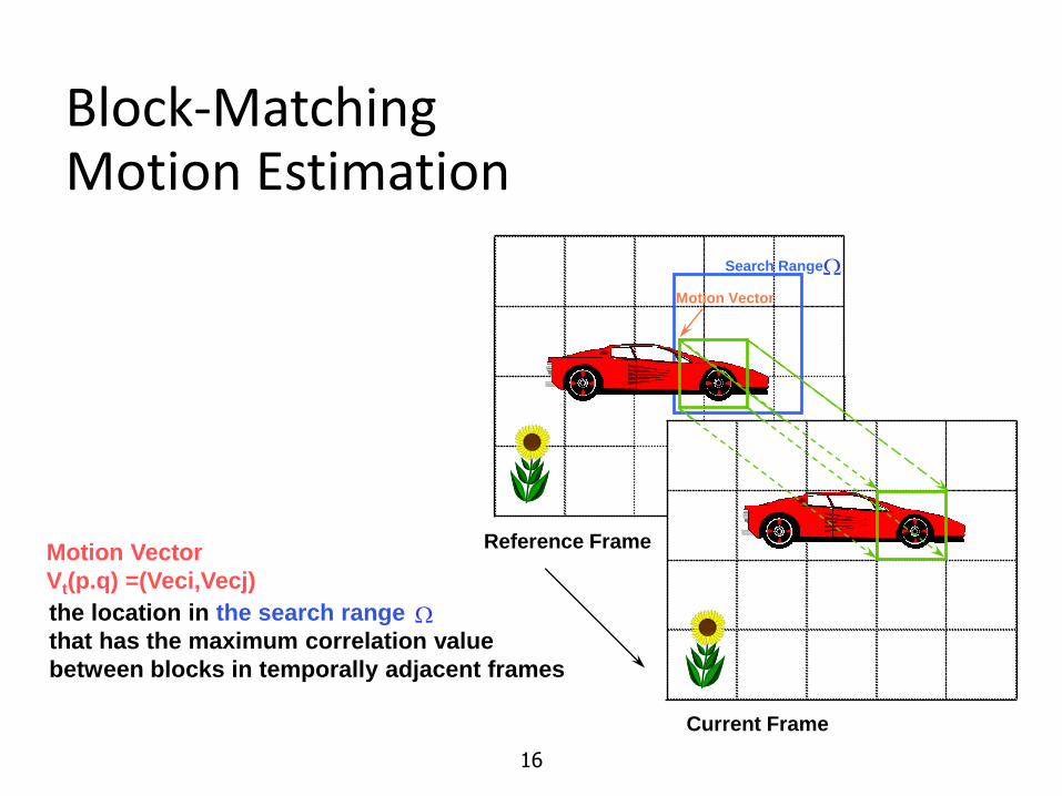
Block-Matching Motion Estimation
Motion Vector
Search Range
Current Frame
Reference FrameMotion Vector
Vt(p.q) =(Veci,Vecj)
the location in the search range
that has the maximum correlation value
between blocks in temporally adjacent frames

Lucas-Kanade Optical Flow
17
Ref: Lucas and Kanade, "An iterative image registration technique with an application to stereo vision," IJCAI, 1981.
To minimize
=

Lucas-Kanade Optical Flow
• Iterative solution
• More dimensions
18
Add weights
Ref: Simon Baker and Iain Matthews, "Lucas-Kanade 20 Years On: A Unifying Framework," IJCV2004.

Lucas-Kanade Algorithm
19
yx
yxTvyuxIvuE,
2),(),(),(
yx vIuIyxIvyuxI ),(),(
yx
yx vIuIyxTyxI,
2),(),(
yx
yxx vIuIyxTyxIIu
E
,
),(),(20
yx
yxy vIuIyxTyxIIv
E
,
),(),(20

Lucas Kanade Algorithm
20
yx
yxx vIuIyxTyxIIu
E
,
),(),(20
yx
yxy vIuIyxTyxIIv
E
,
),(),(20
yx
y
yx
y
yx
yx
yx yx
xyx
yx
x
yxIyxTIvIuII
yxIyxTIvIIuI
,,
2
,
, ,,
2
),(),(
),(),(
yx
y
yx
x
yx
y
yx
yx
yx
yx
yx
x
yxIyxTI
yxIyxTI
v
u
III
III
,
,
,
2
,
,,
2
),(),(
),(),(

Lucas Kanade Algorithm
21
iterate
shift I(x,y) with (u,v)
compute gradient image Ix, Iy
compute error image T(x,y)-I(x,y)
compute Hessian matrix
solve the linear system
(u,v)=(u,v)+(∆u,∆v)
until converge
yx
y
yx
x
yx
y
yx
yx
yx
yx
yx
x
yxIyxTI
yxIyxTI
v
u
III
III
,
,
,
2
,
,,
2
),(),(
),(),(

Lucas Kanade Algorithm: Parametric
22
yx
yxTvyuxIvuE,
2),(),(),(
x
xp)W(x;p2
)()()( TIE
T
yx
y
xddp
dy
dx),(,
p)W(x;translation
T
yxyyyxxyxx
yyyyx
xxyxx
ddddddp
y
x
ddd
ddd
),,,,,(
,
11
1
dAxp)W(x;affine
Our goal is to find
p to minimize E(p)
for all x in T’s domain
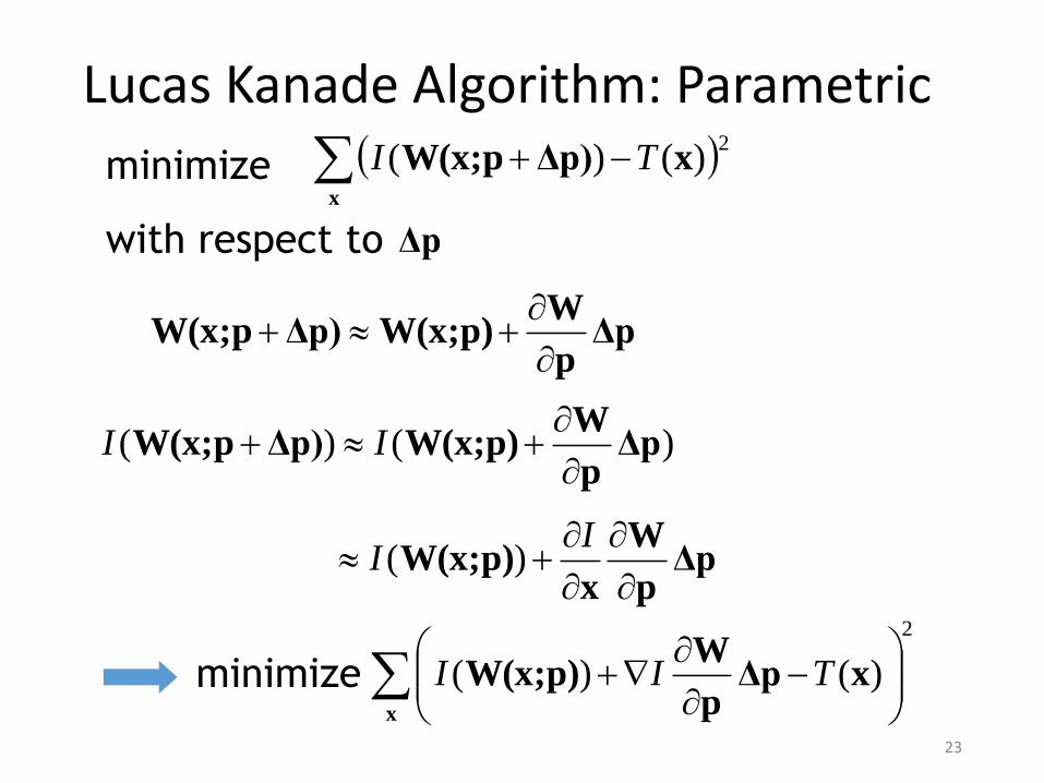
Lucas Kanade Algorithm: Parametric
23
x
xΔp)pW(x;2
)()( TIminimize
with respect to Δp
Δpp
Wp)W(x;Δp)pW(x;
)()( Δpp
Wp)W(x;Δp)pW(x;
II
Δpp
W
xp)W(x;
II )(
x
xΔpp
Wp)W(x;
2
)()( TIIminimize

Lucas Kanade Algorithm: Parametric
24
x
xΔpp
Wp)W(x;
2
)()( TII
image gradient
Jacobian of the warp
warped image
n
yyy
n
xxx
y
x
p
W
p
W
p
W
p
W
p
W
p
W
p
W
p
W
p
W
21
21
target image

Lucas Kanade Algorithm: Parametric
25
For example, for affine
yyyyx
xxyxx
yyyyx
xxyxx
dydxd
dydxdy
x
ddd
ddd
)1(
)1(
11
1p)W(x;
n
yyy
n
xxx
y
x
p
W
p
W
p
W
p
W
p
W
p
W
p
W
p
W
p
W
21
21
1000
0100
yx
yx
p
W
dxx dyx dxy dyy dx dy

Lucas Kanade Algorithm: Parametric
26
x
xΔpp
Wp)W(x;
2
)()( TII
x
xΔpp
Wp)W(x;
p
W)()(0 TIII
T
x
p)W(x;xp
WHΔp )()(1 ITI
T
x p
W
p
WH II
T
(Approximated) Hessian
Δpminarg

Lucas Kanade Algorithm
27
iterate
1) warp I with W(x;p)
2) compute error image T(x,y)-I(W(x,p))
3) compute gradient image with W(x,p)
4) evaluate Jacobian at (x;p)
5) compute
6) compute Hessian
7) compute
8) solve
9) update p by p+
until converge
p
W
p
W
I
x
p)W(x;xp
W)()( ITI
T
Δp
Δp
x
p)W(x;xp
WHΔp )()(1 ITI
T
I

x
p)W(x;xp
WHΔp )()(1 ITI
T

x
p)W(x;xp
WHΔp )()(1 ITI
T

x
p)W(x;xp
WHΔp )()(1 ITI
T

x
p)W(x;xp
WHΔp )()(1 ITI
T

x
p)W(x;xp
WHΔp )()(1 ITI
T

x
p)W(x;xp
WHΔp )()(1 ITI
T

x
p)W(x;xp
WHΔp )()(1 ITI
T

x
p)W(x;xp
WHΔp )()(1 ITI
T

x
p)W(x;xp
WHΔp )()(1 ITI
T

x
p)W(x;xp
WHΔp )()(1 ITI
T

x
p)W(x;xp
WHΔp )()(1 ITI
T

Coarse-to-Fine Strategy
39
J Jw Iwarp refine
ina
a
+
J Jw Iwarp refine
a
a
+
J
pyramid
construction
J Jw Iwarp refine
a
+
I
pyramid
construction
outa

Example
* From Khurram Hassan-Shafique CAP5415 Computer Vision 2003

Multi-resolution registration
* From Khurram Hassan-Shafique CAP5415 Computer Vision 2003

Optical Flow Results
* From Khurram Hassan-Shafique CAP5415 Computer Vision 2003

Optical Flow Results
* From Khurram Hassan-Shafique CAP5415 Computer Vision 2003

Lucas-Kanade Optical Flow
• https://youtu.be/D7r3-fHXvRU?t=1h40m54s
44

Errors of Lucas-Kanade
• The motion is large• Possible Fix: Keypoint matching
• A point does not move like its neighbors• Possible Fix: Region-based matching
• Brightness constancy does not hold• Possible Fix: Gradient constancy
45

Epicflow
• Main remaining problems:• large displacements• occlusions• motion discontinuities
• EpicFlow
Epic: Edge-Preserving Interpolation of Correspondences
• leverages state-of-the-art matching algorithm• invariant to large displacements
• incorporate an edge-aware distance:• handles occlusions and motion discontinuities
• state-of-the-art results
46Ref: J. Revaud, P. Weinzaepfel, Z. Harchaoui and C. Schmid, “EpicFlow: Edge-Preserving Interpolation of Correspondences for Optical Flow,” CVPR 2015.

Epicflow• Problems with coarse-to-fine:
• flow discontinuities overlap at coarsest scales
• errors are propagated across scales
• no theoretical guarantees or proof of convergence!
47
Full-scale estimate Estimation at coarsest scale
Coarsest level (59x26 pixels)1024x436 pixels
EpicFlow

Epicflow: Overview
48
• Avoid coarse-to-fine scheme
(SED)
(DeepMatching)

Epicflow: DeepMatching
• Based on correlation of SIFT features of a patch
49

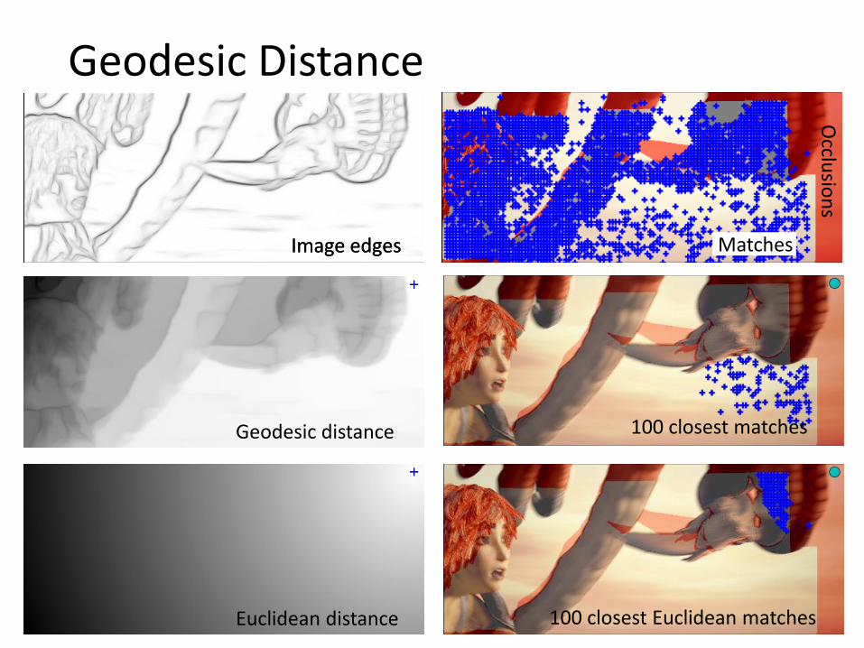
Epicflow: Dense Interpolation
• Replace Euclidean distance with edge-aware distance to find NNs
• Geodesic distance:• Anisotropic cost map =
image edges
►Cost of a path: sum of the cost of all traversed pixels
►Geodesic distance: minimum cost among all possible paths
50
minimum path
q
p

Geodesic Distance
51
Image edges
Geodesic distance
Geodesic distance
100 closest matches
100 closest matches
Occlu
sion
s
Matches
Geodesic Distance
52
Geodesic distance 100 closest matches
Euclidean distance 100 closest Euclidean matches
Image edgesImage edges
Occlu
sion
s
Matches

Experimental Results
53

FlowNet
54
Ref: A. Dosovitskiy, P. Fischer, E. Ilg, P. Hausser, C. Hazirbas, V. Golkov, P. van der Smagt, D. Cremers, T. Brox, “FlowNet: Learning Optical Flow With Convolutional Networks,” CVPR2015.

FlowNet 2.0
55Ref: E. Ilg, N. Mayer, T. Saikia, M. Keuper, A. Dosovitskiy and T. Brox, “FlowNet 2.0: Evolution of Optical Flow Estimation with Deep Networks,” CVPR2017.

Outline
• Tracking• Introduction
• Single camera tracking• Feature tracker, KLT tracker
• Region area tracker• Mean-shift
• Tracking with adaptive filters
• On-line learning
• Multi-camera tracking
56

Introduction to Tracking
57

Introduction to Tracking
• Input: target
• Objective: Estimate target state over time
• State:• Position• Apperance• Shape• Velocity• ...
• It is about data association, similarity measurement, and correlation
58

Feature tracking
• Given two subsequent frames, estimate the point translation
• Key assumptions of Lucas-Kanade Tracker• Brightness constancy: projection of the same point looks the same in
every frame
• Small motion: points do not move very far
• Spatial coherence: points move like their neighbors
I(x,y,t) I(x,y,t+1)

tyx IvIuItyxItvyuxI ),,()1,,(
• Brightness Constancy Equation:
),(),,( 1, tvyuxItyxI
Take Taylor expansion of I(x+u, y+v, t+1) at (x,y,t) to linearize the right side:
The brightness constancy constraint
I(x,y,t) I(x,y,t+1)
0 tyx IvIuISo:
Image derivative along x
0IvuI t
T
tyx IvIuItyxItvyuxI ),,()1,,(
Difference over frames
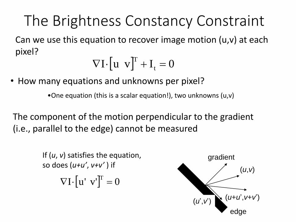
• How many equations and unknowns per pixel?
The component of the motion perpendicular to the gradient (i.e., parallel to the edge) cannot be measured
edge
(u,v)
(u’,v’)
gradient
(u+u’,v+v’)
If (u, v) satisfies the equation, so does (u+u’, v+v’ ) if
•One equation (this is a scalar equation!), two unknowns (u,v)
0IvuI t
T
0'v'uIT
Can we use this equation to recover image motion (u,v) at each pixel?
The Brightness Constancy Constraint

Solving the ambiguity…
• How to get more equations for a pixel?
• Spatial coherence constraint• Assume the pixel’s neighbors have the same (u,v)• If we use a 5x5 window, that gives us 25 equations per pixel
B. Lucas and T. Kanade. An iterative image registration technique with an application to stereo vision. In Proceedings of the International Joint Conference on Artificial Intelligence, pp. 674–679, 1981.
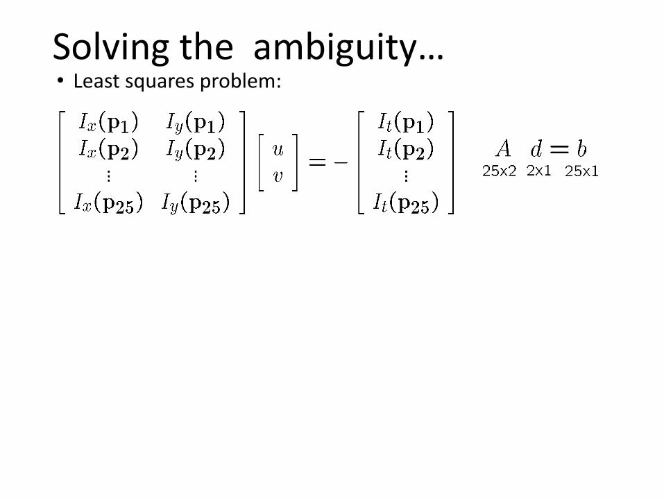
• Least squares problem:
Solving the ambiguity…
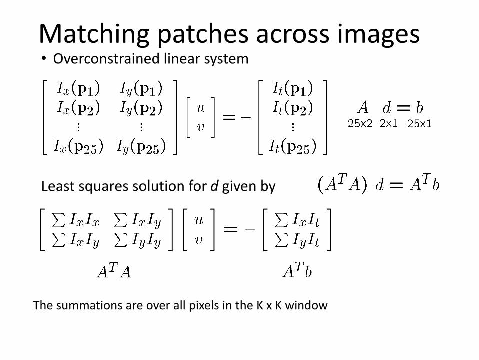
Matching patches across images• Overconstrained linear system
The summations are over all pixels in the K x K window
Least squares solution for d given by
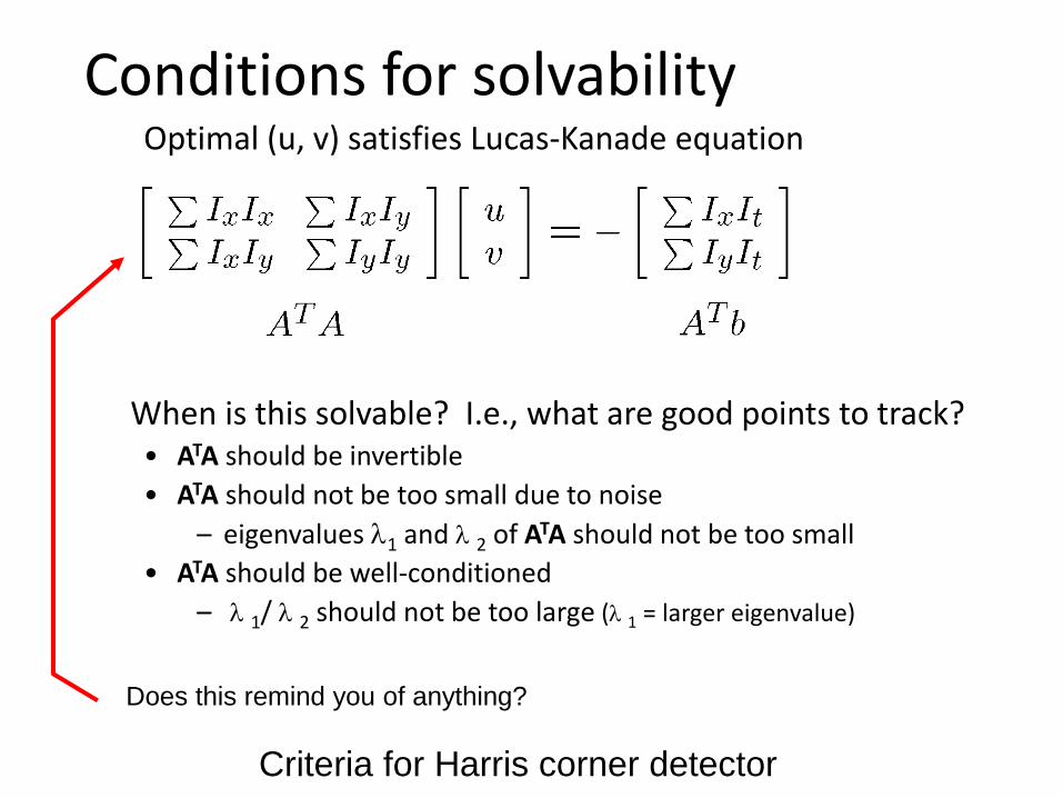
Conditions for solvabilityOptimal (u, v) satisfies Lucas-Kanade equation
Does this remind you of anything?
When is this solvable? I.e., what are good points to track?• ATA should be invertible
• ATA should not be too small due to noise
– eigenvalues 1 and 2 of ATA should not be too small
• ATA should be well-conditioned
– 1/ 2 should not be too large ( 1 = larger eigenvalue)
Criteria for Harris corner detector

Low-texture region
– gradients have small magnitude
– small 1, small 2

Edge
– gradients very large or very small
– large 1, small 2

High-texture region
– gradients are different, large magnitudes
– large 1, large 2

Dealing with Larger Movements: Iterative Refinement
1. Initialize (x’,y’) = (x,y)
2. Compute (u,v) by
3. Shift window by (u, v): x’=x’+u; y’=y’+v;
4. Recalculate It
5. Repeat steps 2-4 until small change• Use interpolation for subpixel values
2nd moment matrix for feature
patch in first imagedisplacement
It = I(x’, y’, t+1) - I(x, y, t)
Original (x,y) position

image Iimage J
Gaussian pyramid of image 1 (t) Gaussian pyramid of image 2 (t+1)
image 2image 1
Dealing with Larger Movements: Coarse-to-Fine Registration
run iterative L-K
run iterative L-K
upsample
.
.
.

Shi-Tomasi Feature Tracker• Find good features using eigenvalues of second-
moment matrix (e.g., Harris detector or threshold on the smallest eigenvalue)• Key idea: “good” features to track are the ones whose
motion can be estimated reliably
• Track from frame to frame with Lucas-Kanade• This amounts to assuming a translation model for frame-to-
frame feature movement
• Check consistency of tracks by affine registration to the first observed instance of the feature• Affine model is more accurate for larger displacements• Comparing to the first frame helps to minimize drift
Ref: J. Shi and C. Tomasi. Good Features to Track. CVPR 1994.

Tracking example
Ref: J. Shi and C. Tomasi. Good Features to Track. CVPR 1994.

Summary of KLT tracking
• Find a good point to track (harris corner)
• Use intensity second moment matrix and difference across frames to find displacement
• Iterate and use coarse-to-fine search to deal with larger movements
• When creating long tracks, check appearance of registered patch against appearance of initial patch to find points that have drifted
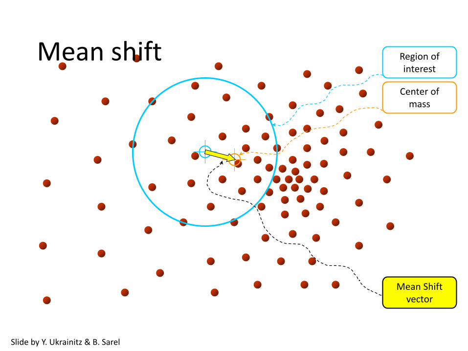
Region ofinterest
Center ofmass
Mean Shiftvector
Slide by Y. Ukrainitz & B. Sarel
Mean shift
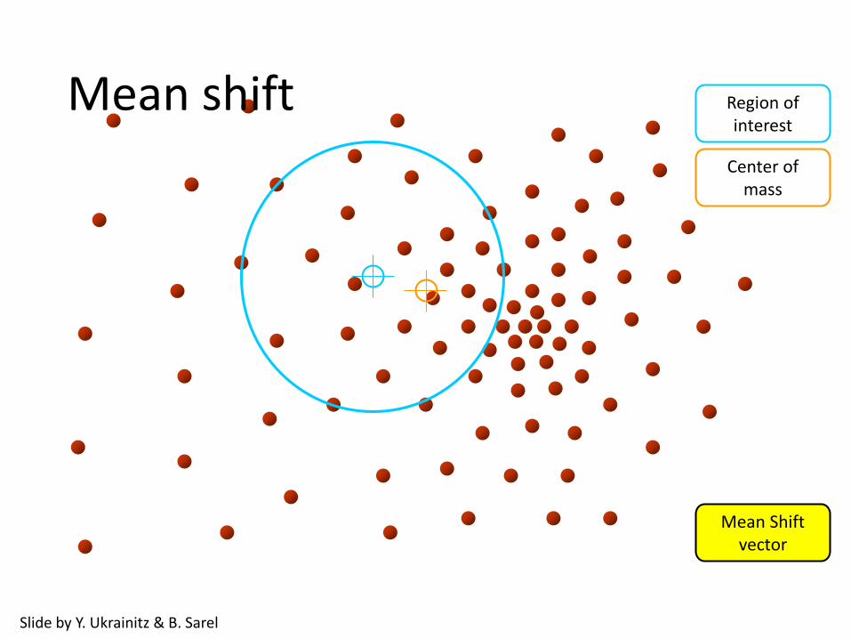
Region ofinterest
Center ofmass
Mean Shiftvector
Slide by Y. Ukrainitz & B. Sarel
Mean shift

Region ofinterest
Center ofmass
Mean Shiftvector
Slide by Y. Ukrainitz & B. Sarel
Mean shift

Region ofinterest
Center ofmass
Mean Shiftvector
Mean shift
Slide by Y. Ukrainitz & B. Sarel

Region ofinterest
Center ofmass
Mean Shiftvector
Slide by Y. Ukrainitz & B. Sarel
Mean shift

Region ofinterest
Center ofmass
Mean Shiftvector
Slide by Y. Ukrainitz & B. Sarel
Mean shift

Region ofinterest
Center ofmass
Slide by Y. Ukrainitz & B. Sarel
Mean shift

Simple Mean Shift procedure:
• Compute mean shift vector
•Translate the Kernel window by m(x)
2
1
2
1
( )
ni
i
i
ni
i
gh
gh
x - xx
m x xx - x
Computing the Mean Shift
Slide by Y. Ukrainitz & B. Sarel
82
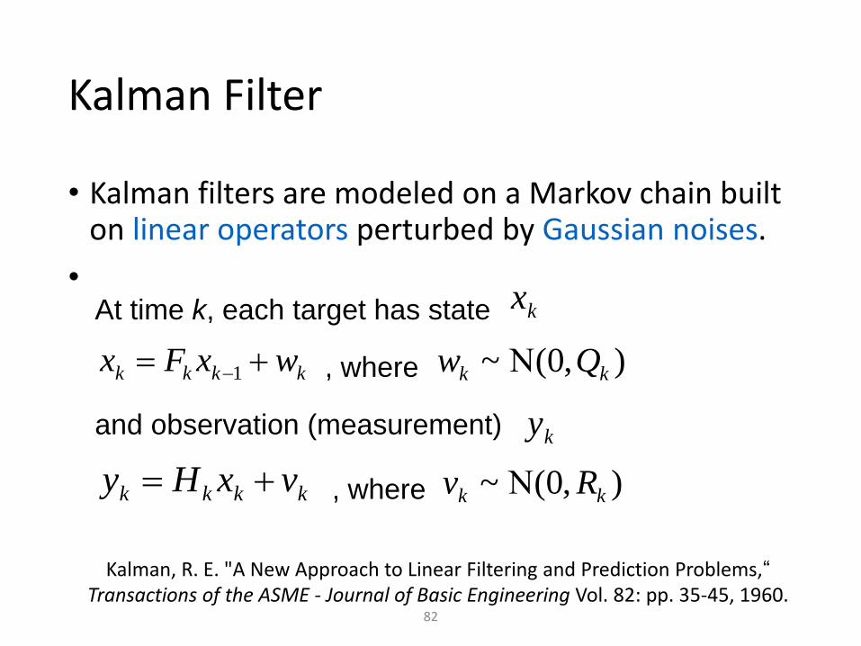
Kalman Filter
• Kalman filters are modeled on a Markov chain built on linear operators perturbed by Gaussian noises.
•
kkkk wxFx 1
At time k, each target has state
kkkk vxHy
and observation (measurement)
kx
ky
),0(~ kk Qw , where
, where ),0(~ kk Rv
Kalman, R. E. "A New Approach to Linear Filtering and Prediction Problems,“Transactions of the ASME - Journal of Basic Engineering Vol. 82: pp. 35-45, 1960.
83
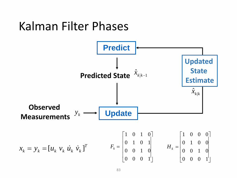
Kalman Filter Phases
Predict
Update
Predicted State
Observed Measurements
1ˆ
kkx
ky
Updated State
Estimate
kkx |ˆ
1000
0100
0010
0001
kH
1000
0100
1010
0101
kFT
kkkkkk vuvuyx ][

84
Kalman Filter Phases
Predict PhaseUpdate Phase
k
T
kkkkkk
kkkkk
QFPFP
xFx
111
111ˆˆ
• Predicted Estimate
Covariance
• Predicted State kkkkkk yKxx ~ˆˆ1||
• Updated State Estimate
• Updated Estimate Covariance
• Kalman Gain
• Innovation (Measurement) Residual
• Innovation Covariance
1
1|
k
T
kkkk SHPK
1|| )( kkkkkk PHKIP
k
T
kkkkk RHPHS 1|
1|ˆ~
kkkkk xHyy
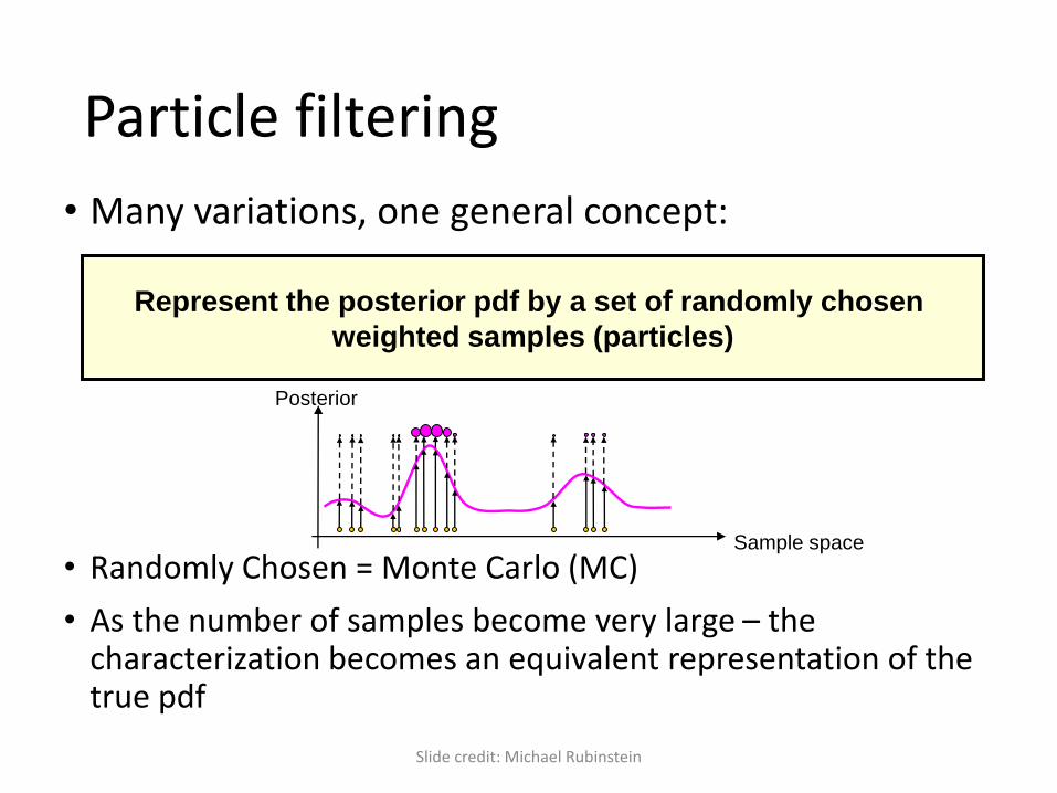
Particle filtering
• Many variations, one general concept:
• Randomly Chosen = Monte Carlo (MC)
• As the number of samples become very large – the characterization becomes an equivalent representation of the true pdf
Represent the posterior pdf by a set of randomly chosen
weighted samples (particles)
Slide credit: Michael Rubinstein
Sample space
Posterior

Generic PF
},{ 1Nxi
k
},{ k
i
k wx
},{ 1* Nxi
k
},{ 1
1
Nxi
k
},{ 11 k
i
k wxVan der Merwe et al.
Uniformly weighted measure
Approximates )|( 1:1 kk zxp
Compute for each particle
its importance weight to
Approximate
(Resample if needed)
Project ahead to approximate
)|( :11 kk zxp
)|( :1 kk zxp
)|( 1:11 kk zxp© Michael Rubinstein

Particle Filter • Try to approximate p(X |Zt)
• Sampling → evaluation → resampling

On-line Learning
• Discriminative modeling (tracking-by-detection)
• Learn and apply a detector or predictor
• Challenges:• What are the training data? Label?
• How to avoid drift? Handle occlusion?
• How to control complexity?
88

On-line Learning
89

On-line Learning
• On-line discriminative learning
• One-shot learning
• On-line update of the classifier
90
Grabner and Bischof CVPR06

On-line Learning
• Examples of on-line discriminative learning – Multiple Instance Learning [1] – Kernelized Structured SVM [2] – Combine short track + detector [3]
91
[1] Babenko, Boris, Ming-Hsuan Yang, and Serge Belongie. "Visual tracking with online multiple instance learning." CVPR 2009 [2] Hare, Sam, Amir Saffari, and Philip HS Torr. "Struck: Structured output tracking with kernels.” ICCV 2011 [3] Kalal, Zdenek, KrysEan Mikolajczyk, and Jiri Matas. "Tracking-learning-detection." PAMI 2012

On-line Learning
• Example: TLD
92
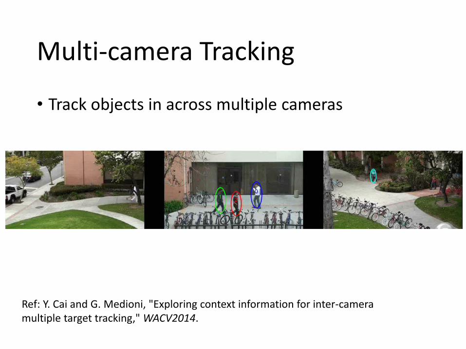
Multi-camera Tracking
• Track objects in across multiple cameras
Ref: Y. Cai and G. Medioni, "Exploring context information for inter-camera multiple target tracking," WACV2014.
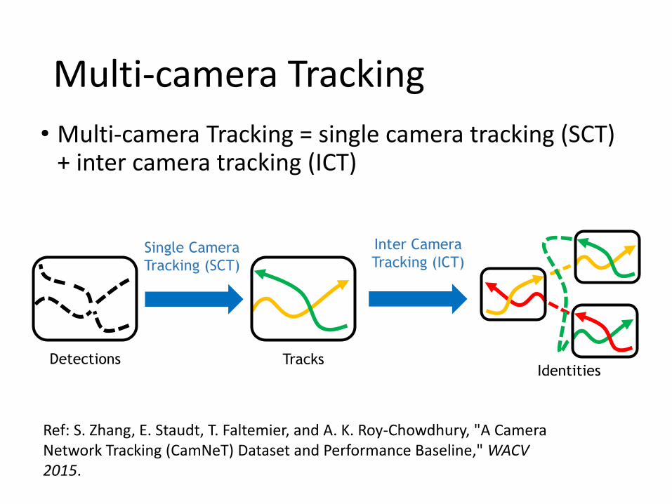
Multi-camera Tracking
Detections TracksIdentities
Single Camera
Tracking (SCT)
Inter Camera
Tracking (ICT)
Ref: S. Zhang, E. Staudt, T. Faltemier, and A. K. Roy-Chowdhury, "A Camera Network Tracking (CamNeT) Dataset and Performance Baseline," WACV 2015.
• Multi-camera Tracking = single camera tracking (SCT) + inter camera tracking (ICT)

Multi-camera Tracking
• Applications• Surveillance camera network
• Customer flow analysis
• Homeland security
• Monitoring of elders, children, and patients
• Crime prevention
• Traffic control
• …

Re-identification
Same person?

Re-identification
• is not an easy task…

The Relationship of Multi-camera Tracking and Re-identification
• Multi-camera tracking framework
Ref: X. Wang, “Intelligent multi-camera video surveillance: a review,”Pattern recognition letters, vol. 34, no. 1, pp. 3–19, 2013.
An important part of multi-camera tracking

The Relationship of Multi-camera Tracking and Re-identification
• History of re-identification
Ref: L. Zheng, Y. Yang, and A. G. Hauptmann, “Person reidentification: Past, present and future,” arXiv preprint arXiv:1610.02984, 2016.
The first time image re-identification became an independent computer vision task
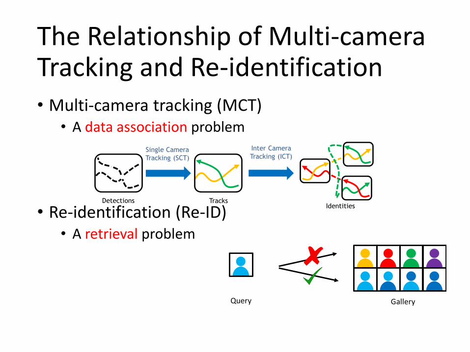
The Relationship of Multi-camera Tracking and Re-identification• Multi-camera tracking (MCT)
• A data association problem
• Re-identification (Re-ID)• A retrieval problem
Detections TracksIdentities
Single Camera
Tracking (SCT)
Inter Camera
Tracking (ICT)
Query Gallery

Distributed Multi-Camera Tracking
• Centralized approach or distributed approach?
• Distributed computing is a more efficient approach to deal with such ultra-big data Cloud Servers
AggregatorAggregator
Smart Devices
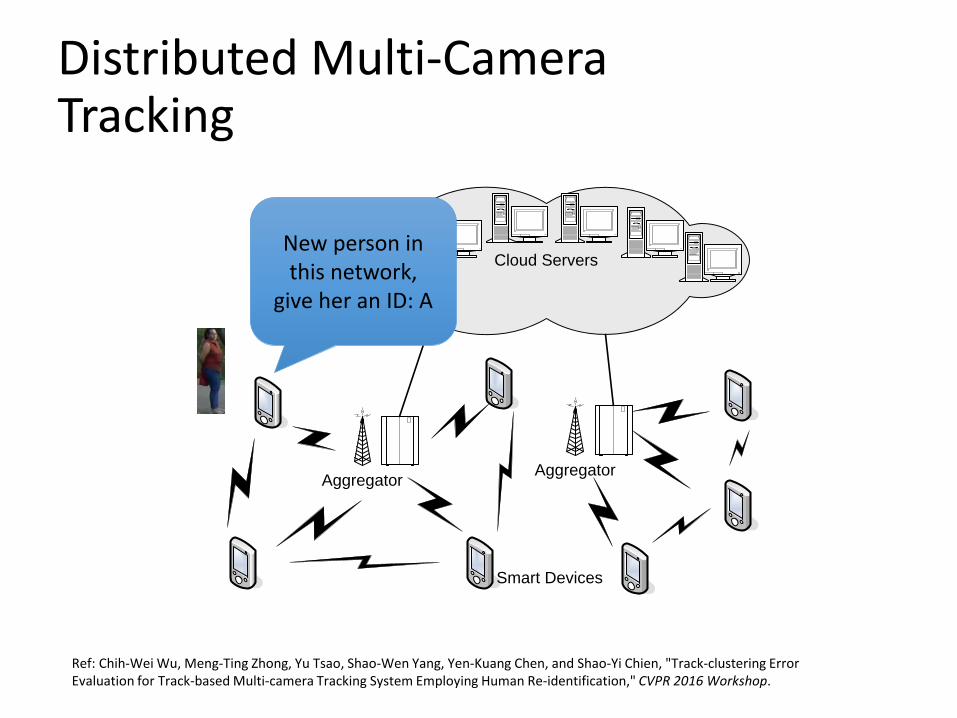
Distributed Multi-Camera Tracking
Cloud Servers
AggregatorAggregator
Smart Devices
New person in this network,
give her an ID: A
Ref: Chih-Wei Wu, Meng-Ting Zhong, Yu Tsao, Shao-Wen Yang, Yen-Kuang Chen, and Shao-Yi Chien, "Track-clustering Error Evaluation for Track-based Multi-camera Tracking System Employing Human Re-identification," CVPR 2016 Workshop.

Distributed Multi-Camera Tracking
Cloud Servers
AggregatorAggregator
Smart Devices
Person A is now appearing in my
view
Ref: Chih-Wei Wu, Meng-Ting Zhong, Yu Tsao, Shao-Wen Yang, Yen-Kuang Chen, and Shao-Yi Chien, "Track-clustering Error Evaluation for Track-based Multi-camera Tracking System Employing Human Re-identification," CVPR 2016 Workshop.
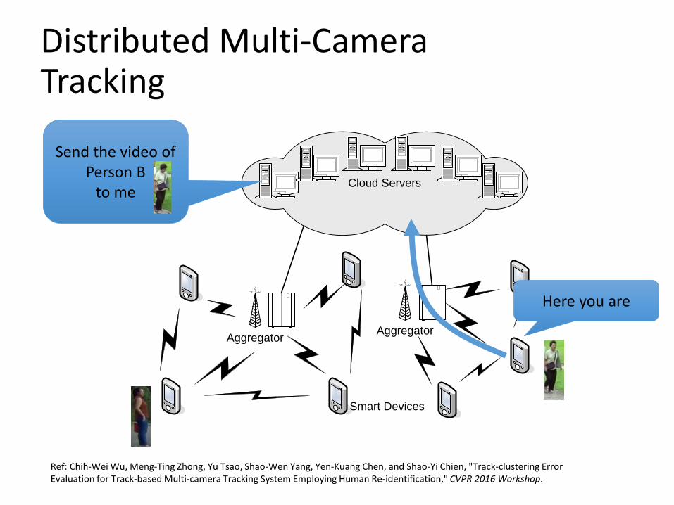
Distributed Multi-Camera Tracking
Cloud Servers
AggregatorAggregator
Smart Devices
Send the video of Person B
to me
Here you are
Ref: Chih-Wei Wu, Meng-Ting Zhong, Yu Tsao, Shao-Wen Yang, Yen-Kuang Chen, and Shao-Yi Chien, "Track-clustering Error Evaluation for Track-based Multi-camera Tracking System Employing Human Re-identification," CVPR 2016 Workshop.


![Diffuse Skeletal Muscles Uptake of [18F] …...2021 CASE REPORT Diffuse Skeletal Muscles Uptake of [18F] Fluorodeoxyglucoseon Positron Emission Tomography in Primary Muscle Peripheral](https://img.pdfslide.tips/doc/110x75/5e447f1d6101324fdb79c19f/diffuse-skeletal-muscles-uptake-of-18f-2021-case-report-diffuse-skeletal-muscles.jpg)


![Ruolo dell’imaging nella diagnosi differenziale delle ... · PET amiloide: [11C] PiB-PET, Florbetapir F18 Tau scan: 18F-T807 PET, 18F-THK523 PET BF227 α-synuclein/Lewy bodies PET](https://img.pdfslide.tips/doc/110x75/5f5d423cb091ea08670bd90e/ruolo-dellaimaging-nella-diagnosi-differenziale-delle-pet-amiloide-11c.jpg)
![Procedures for the GMP-Compliant Production and 18F]PSMA](https://img.pdfslide.tips/doc/110x75/616dfb8fdb4b332e2e748c4b/procedures-for-the-gmp-compliant-production-and-18fpsma-.jpg)


![18F]Flubatine as a novel α4β2 nicotinic acetylcholine](https://img.pdfslide.tips/doc/110x75/629737326d4e5a451c0d4cae/18fflubatine-as-a-novel-42-nicotinic-acetylcholine-.jpg)