OPTICAL PROPERTIES OF INORGANIC SUSPENDED SOLIDS …€¦ · OPTICAL PROPERTIES OF INORGANIC SUSPENDED SOLIDS AND THEIR INFLUENCE ON COASTAL OCEAN COLOR REMOTE SENSING H. Kobayashi

OPTICAL PROPERTIES OF INORGANIC SUSPENDED SOLIDS AND THEIR

INFLUENCE ON COASTAL OCEAN COLOR REMOTE SENSING

H. Kobayashi a, *, M. Toratani b, S. Matsumura c, A. Siripong d, T. Lirdwitayaprasit d, P. Jintasaeranee e

a Interdis. Grad. School Med. Eng., Univ. Yamanashi, Kofu, Japan - [email protected]

b School High Tech. Human Welfare, Tokai Univ., Numazu, Japan c National Research Institute of Far Seas Fisheries, Shizuoka, Japan

d Faculty of Science, Chulalongkorn Univ., Bangkok, Thailand e Faculty of Science, Burapha University, Chonburi, Thailand

Working Group VIII/9 - Oceans

KEY WORDS: Ocean color remote sensing, inorganic suspended solids, in-water algorithm, red and infrared bands ABSTRACT:S

The influence of the optical properties of inorganic suspended solids (ISS) on in-water algorithms was evaluated using an optical model in highly turbid coastal water, whose ISS concentration reached several hundred grams per cubic metre. The measurements were conducted in the upper Gulf of Thailand. The backscattering coefficient of the ISS was calculated using the Lorenz–Mie scattering theory. On the basis of the measurement, the ISS size distribution was parameterised as a function of ISS concentration, and both the spherical and non-spherical particle shape models were evaluated. For ISS concentrations of 10 g m-3, an estimate of the chlorophyll-a (Chl-a) concentration within a factor of two on a logarithmic scale is possible in a Chl-a range of 4–30 mg m-3.

* Corresponding author.

1. INTRODUCTION

Coastal waters, which have high productivity and which are strongly affected by human activities, suffer from many environmental problems. Environmental monitoring of coastal waters is necessary. Ocean color remote sensing is an effective monitoring method. Estimation errors occur when applying algorithms of remote sensing to coastal waters because high abundances of suspended solids (SS) and colored dissolved organic matter (CDOM) increase the waters’ optical complexity. Particularly in coastal waters, nonliving particulate matter, which mostly comprises mineral particles or inorganic suspended solids (ISS), is dominant in scattering processes in water. Such matter has a high refractive index and absorbs light of shorter wavelengths. It is important to quantify the applicable coverage using ocean color remote sensing in highly turbid coastal waters. For this study, we calculate the ISS backscattering coefficient based on scattering theory for spherical particles, including huge particles, using the Lorenz–Mie method. For the scattering calculation, the size distribution and the complex refractive index of particles are required. In this study, the ISS size distribution, including the size range, is measured from water samples from highly turbid coastal waters in which the ISS concentration is as high as several hundred grams per cubic metre. The ISS size distribution is parameterised as a function of the ISS concentration. The real part of the complex refractive index of ISS is assumed as some commonly used value. The imaginary part is derived from measurements of the size distribution and the absorption coefficient, using the Mie theory. Additionally, we examine the influence of derived IOPs of ISS on two algorithms––the SeaWiFS standard, and local empirical algorithms––and evaluate the applicable estimation range of the Chl-a concentration in highly turbid coastal waters.

100˚00' 100˚30' 101˚00'E

12˚30'

13˚00'

13˚30'N

G3G4

G5

G6

G7 G8 G9

G11 G12 G13

G14

G16

100˚45' 101˚00'E

13˚15'

13˚30'N

B6,G1G2

G17

B1

B2B3B4

B5B7

B8B9

Bangpankong River

+Chon Buri

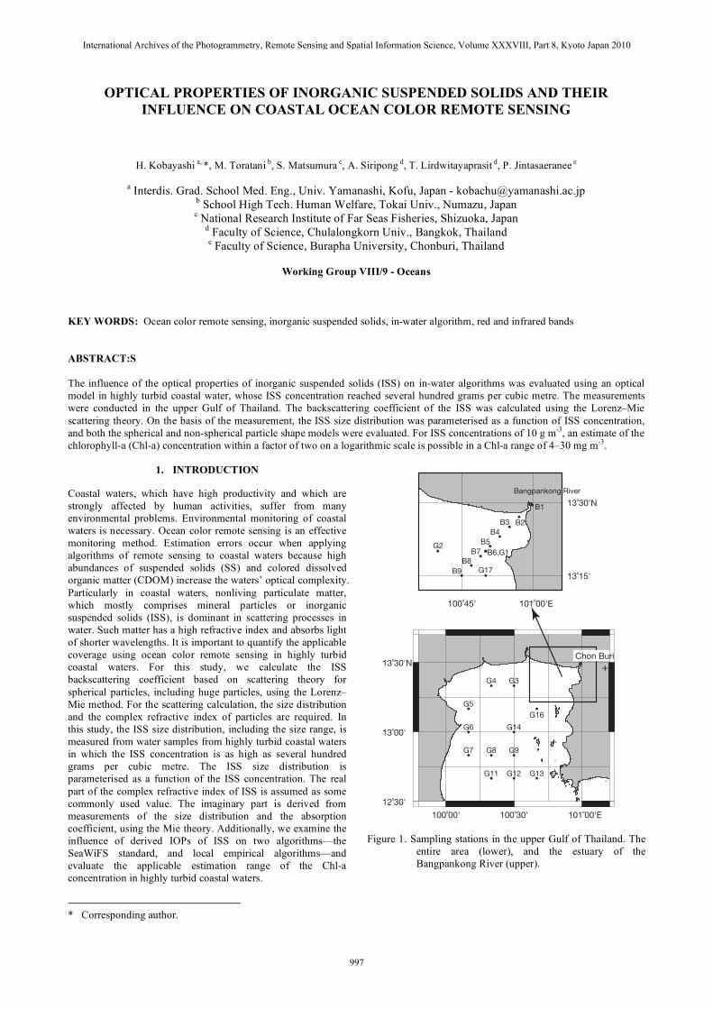
Figure 1. Sampling stations in the upper Gulf of Thailand. The

entire area (lower), and the estuary of the Bangpankong River (upper).

International Archives of the Photogrammetry, Remote Sensing and Spatial Information Science, Volume XXXVIII, Part 8, Kyoto Japan 2010

997

2. SAMPLING AND METHODS

2.1 Measurements

Observations were performed throughout the entire area of the upper Gulf of Thailand during May 2004; additional observations were made during May 2005 around the estuary of the Bangpankong River, northeast of the upper gulf, where the water exhibits high turbidity and optical diversity (figure 1). During the 2005 cruise, observations at some sampling stations were repeated on another day. Results of the second observation are denoted with the station number and (2). Transparency was measured using a Secchi disk, and is represented as the reading depth. Spectral upward radiance and downward irradiance in water were measured at each depth using submersible radiometers (RAMSES ACC/ARC; TriOS Optical Sensors) equipped with depth meters. The measured radiance and irradiance were calibrated using immersion factors (Zibordi and Darecki, 2006). Moreover, the self-shading of the radiometers that measured upward radiance was corrected using equations described in Mueller (Muller, 2003).. Water samples were collected from the surface using a Van Dorn sampler in 2004, and using a bucket in 2005. For each sample, six separate samples were filtered for the following purposes. (1) The water sample was filtered onto a glass fibre filter (25 mm GF/F; Whatman plc.). The Chl-a concentration was determined fluorometrically using a fluorometer (10-000R; Turner Designs Inc.) after extracting the pigments in N,N-dimethylformamide (Suzuki and Ishimaru, 1990). (2) The SS concentration was measured using a 47 mm GF/F filter (Whatman plc.). The filter was gently rinsed with distilled water to remove residual salt. After measuring the total SS weight, the GF/F filter was pre-processed at 500°C for 2 h to remove organic components. The ignition loss was considered as organic suspended solids (OSS). The difference between the total SS and the OSS was considered as the ISS amount. The artificial loss of mass occurs by leaching into the fibres, and the artificial addition of mass is attributable to the remnant sea salt and water of hydration on the GF/F filter. This retention of salt and the water of hydration on the filters was therefore estimated from salinity (Stavn et al., 2009), and was subtracted from the weight of the filtered GF/F filter. The estimated water of hydration retention was subtracted from that of the ashed GF/F filter. Ignition loss includes the loss of structural water from clay minerals in the ignition process (BarillÈ-Boyer et al., 2003). Therefore, the loss of structural water was also estimated from the clay fraction of the ISS and the composition ratio of each clay mineral, and was corrected to the weight of the ashed GF/F filter. Because we did not conduct a mineralogical analysis of the gathered suspended particles, the clay fraction and composition ratio were estimated from measurements of Thai paddy soils in Chon Buri (Prakongkep et al., 2008), which is located near the Bangpankong River (figure 1). The values of the composition ratios of the kaolinite and illite used were 27% and 16% of the ISS amount, respectively. (3) The particles were collected onto a 25 mm GF/F filter and stored in liquid nitrogen to determine the absorption coefficient of the phytoplankton. The optical density of the particles was measured using a spectrophotometer (V-550; Jasco Inc.) equipped with an integrating sphere (Mitchell, 1990) (ISV-469; Jasco Inc.). The absorption coefficient was calculated from the

measured optical density of the filter sample using the path length amplification factor (Cleveland and Weidemann, 1993; Kishino et al., 1985). Results showed that the absorption of non-living particles such as mineral particles was dominant around the Bangpankong River estuary, where observations were conducted during the 2005 cruise. Therefore, this measurement was conducted using only samples taken during the 2004 cruise. (4) The ISS absorption coefficient was measured using the same procedure as that used for the absorption coefficient of the phytoplankton. However, the glass fibre filter was heated at 500 °C for 2 h before optical density measurements. (5) The absorption coefficient of CDOM was measured using the spectrophotometer with a 10-cm long cell from the water sample, which was filtered using a 47 mm polycarbonate filter with a 0.2-μm pore size (Nuclepore; Whatman plc.). (6) For analyses of the ISS size distribution, the water sample was filtered onto a low-ash membrane filter (47 mm Cellulose acetate; Toyo Roshi Kaisha Ltd.), after which it was put on an evaporating dish and heated at 500 °C for 2 h. The remaining particles on the evaporating dish were suspended in a solution of Na3PO4. The size distribution was measured using a Coulter counter (Multisizer 3; Beckman Coulter Inc.) equipped with a 70-μm-diameter aperture whose range of measurement was 1.4–42 μm in diameter. The Coulter counter measures particle volume directly. Therefore, the size represents the equivalent sphere diameter. The particles included in samples collected near and inside the river mouth were larger than the aperture size. For this reason, the size of the aperture tube was changed to 280 or 400 μm, and these measured a diameter size range of 5.6–168 μm and 8.0–240 μm, respectively. Blank samples were obtained in which the seawater had been filtered. Detection limits were fixed at the standard deviation of the measurement of the blank samples for each size bin.

3. RESULTS AND DISCUSSION

3.1 Estimation of bbISS( )

The ISS backscattering coefficient bbISS( ) was calculated based on scattering theories. For size-dispersed particles, the backscattering coefficient is written as

b

bISS( ) =

4N (D)Q

bb( , D)D2 dD

Dmin

Dmax

(1)

where N(D)dD is the number concentration in the size interval from D to D + dD, Qbb( ,D) is the efficiency factor of backscattering, and Dmin and Dmax represent the maximum and minimum diameter, respectively, of the size distribution. N(D), which has a concentration unit, is calculated using the measured ISS concentration, as follows:

N (D) =ISS

ISS 6n

0(D)D

3dD

Dmin

Dmax

n0(D)

(2)

where n0(D) is the number–size distribution, and ISS is the density of ISS as 2.65 g cm-3. In this study, n0(D) was estimated from a size distribution model that was constructed based on the measured ISS size distributions.


998

0.001

0.01

0.1

1

10

100

1 10 100 200

dN

(D)/

dln

(D) (

mm

-3)

Equivalent sphere diameter (μm)

> 200

> 100

> 10

> 1

> 2

> 0.2

> 0.8

ISS conc. (g m-3)

≤ 0.2

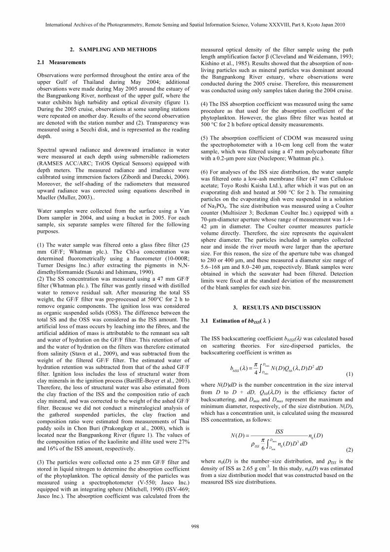
Figure 2. Measured number–size distributions of ISS at each

sampling station.

0.001

0.01

0.1

1

10

100

1000

10000

1 10 100 200

dN

(D)/

dln

(D) (

mm

-3)

Equivalent sphere diameter (μm)

Measured2CLognormalSum

Figure 3. ISS size distribution at Station B4. The size

distribution is fitted to the sum (red line) of a two-component distribution (orange line) and a lognormal distribution (green line).

Figure 2 portrays the measured ISS number–size distributions. Most notably, none of the distributions on the log–log plot are straight; rather, each is a convex curve. Risovi presented a two-component (2C) model based on the combination of two generalised gamma functions for marine particle size distribution (Risovi , 1993). The 2C model was applied to the measured ISS size distribution. The shape and mode diameter of the generalised gamma function are sensitive to variation of their parameters, which are and . Those of the lognormal distribution, on the other hand, are not so sensitive. The meaning of their parameters, namely mode diameter and geometric standard deviation, are easy to understand. Consequently, the ISS size distribution is assumed to be consistent with the original 2C model and the lognormal distributions. The 2C model parameters used the values proposed by Risovi (Risovi , 2002), which are A = 0.137, B = 0.226, and CA/CB = 1016. Therefore, the n0(D) used in this study is expressed as shown below.

n0 (D) = C2C FA (D)+1016FB (D)( )

+Clognormal

Dexp

(ln(D) ln(Dm ))2

2 ln2 ( g ),

FA (D) = D2 4 exp 52 D 2( )

0.137( ),

FB (D) = D2 4 exp 17 D 2( )

0.226( )., (3)

0.001

0.01

0.1

1

0.1 1 10 100

bb

(m-1)

ISS concentration (mg m-3)

565 nm670 nm865 nm

Figure 4. Backscattering coefficient of ISS at 565 nm, 670 nm,

and 865 nm. In this equation Dm is the mode diameter, g is the geometric standard deviation, and C2C and Clognormal signify the arbitrary constants of the 2C model, and lognormal distributions, respectively. The measured ISS size distributions were fitted with equation (3) to determine these parameters. Figure 3 shows the result of curve fitting at Stn. 4 as an example. The four derived parameters––the ratio of Clognormal to C2C, the mode diameter Dm, the geometric standard deviation g, and maximum diameter Dmax––vary in relation to changes in the ISS concentration. These parameters were therefore parameterised with the ISS concentration. The minimum diameter cannot be measured because the lower limit of detection size of the Coulter counter equipped with the aperture used for this study is 1.4 μm, and particles of similar size were present in sufficient numbers. Resovi (2002) reported that the backscattering ratios for the 2C model, and the Junge distribution, become constant as Dm is lower than 0.06, and 0.02 μm, respectively. Consequently, the Dm was assumed as 0.02 μm. The efficiency factor of backscattering is calculated as

Qbb ( ,D) =P( ,D, )sin d

/2

P( ,D, )sin d0

Qb ( ,D)

, (4)

where P( ,D, ) is the phase function, is the scattering angle, and Qb( ,D) is the scattering efficiency factor. Both P( ,D, ) and Qb( ,D) can be calculated using scattering theories by approximating the particle shape to a simple numerical model. The ISS particles are irregularly shaped; they are not spherical. Assuming spherical ISS particles, the Lorenz–Mie method (LM) (Tanré et al., 2001) was used for this study. The LM code was downloaded (Mishchenko et al.) and modified. The calculation of scattering theories requires the use of a complex refractive index of the particle, which comprises both real and imaginary parts. The real part of ISS was assumed to be 1.51 in air, which is a typical value of mineral particles (Sokolik and Toon, 1999). The imaginary part of the ISS was estimated using trial and error until it agreed with the measured aISS( ) at each sampling station, in each wavelength with that calculated using the Mie theory with the measured ISS size distribution, the assumed real part, and the variable imaginary part. The look-up table of Qbb( ,D) was calculated for wavelengths from 350–900 nm in 10 nm increments, and with 375 points of diameter from 0.01 μm to 200 μm. These results are consistent


999

ISS concentration (g m-3)

0.1

0.3

1

3

10

30

100

1

10

50

Est

imat

ed C

hl-a

con

c. (m

g m

-3)

1

10

50

(1) Empirical algorithm for Gulf of Thailand (GT)

(2) SeaWiFS OC4v4 algorithm (OC4)

Est

imat

ed C

hl-a

con

c. (m

g m

-3)

50

Assumed Chl-a concentration (mg m-3)

1 10 501 10 501 10

50

Assumed Chl-a concentration (mg m-3)

1 10 501 10 501 10

(a) aCDOM(440) = 0.1 (m-1) (b) aCDOM(440) = 0.2 (m-1) (c) aCDOM(440) = 0.4 (m-1)

(f) aCDOM(440) = 0.4 m-1(e) aCDOM(440) = 0.2 m-1(d) aCDOM(440) = 0.1 (m-1)

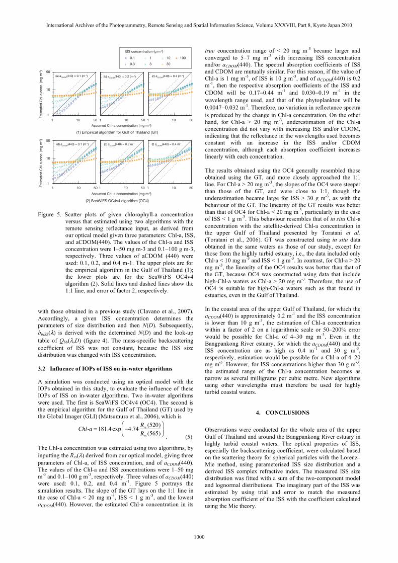
Figure 5. Scatter plots of given chlorophyll-a concentration

versus that estimated using two algorithms with the remote sensing reflectance input, as derived from our optical model given three parameters: Chl-a, ISS, and aCDOM(440). The values of the Chl-a and ISS concentration were 1–50 mg m-3 and 0.1–100 g m-3, respectively. Three values of aCDOM (440) were used: 0.1, 0.2, and 0.4 m-1. The upper plots are for the empirical algorithm in the Gulf of Thailand (1); the lower plots are for the SeaWiFS OC4v4 algorithm (2). Solid lines and dashed lines show the 1:1 line, and error of factor 2, respectively.

with those obtained in a previous study (Clavano et al., 2007). Accordingly, a given ISS concentration determines the parameters of size distribution and then N(D). Subsequently, bbISS( ) is derived with the determined N(D) and the look-up table of Qbb( ,D) (figure 4). The mass-specific backscattering coefficient of ISS was not constant, because the ISS size distribution was changed with ISS concentration. 3.2 Influence of IOPs of ISS on in-water algorithms

A simulation was conducted using an optical model with the IOPs obtained in this study, to evaluate the influence of these IOPs of ISS on in-water algorithms. Two in-water algorithms were used. The first is SeaWiFS OC4v4 (OC4). The second is the empirical algorithm for the Gulf of Thailand (GT) used by the Global Imager (GLI) (Matsumura et al., 2006), which is

Chl-a = 181.4 exp 4.74

Rrs (520)

Rrs (565) . (5)

The Chl-a concentration was estimated using two algorithms, by inputting the Rrs( ) derived from our optical model, giving three parameters of Chl-a, of ISS concentration, and of aCDOM(440). The values of the Chl-a and ISS concentrations were 1–50 mg m-3 and 0.1–100 g m-3, respectively. Three values of aCDOM(440) were used: 0.1, 0.2, and 0.4 m-1. Figure 5 portrays the simulation results. The slope of the GT lays on the 1:1 line in the case of Chl-a < 20 mg m-3, ISS < 1 g m-3, and the lowest aCDOM(440). However, the estimated Chl-a concentration in its

true concentration range of < 20 mg m-3 became larger and converged to 5–7 mg m-3 with increasing ISS concentration and/or aCDOM(440). The spectral absorption coefficients of ISS and CDOM are mutually similar. For this reason, if the value of Chl-a is 1 mg m-3, of ISS is 10 g m-3, and of aCDOM(440) is 0.2 m-1, then the respective absorption coefficients of the ISS and CDOM will be 0.17 0.44 m-1 and 0.030 0.19 m-1 in the wavelength range used, and that of the phytoplankton will be 0.0047 0.032 m-1. Therefore, no variation in reflectance spectra is produced by the change in Chl-a concentration. On the other hand, for Chl-a > 20 mg m-3, underestimation of the Chl-a concentration did not vary with increasing ISS and/or CDOM, indicating that the reflectance in the wavelengths used becomes constant with an increase in the ISS and/or CDOM concentration, although each absorption coefficient increases linearly with each concentration. The results obtained using the OC4 generally resembled those obtained using the GT, and more closely approached the 1:1 line. For Chl-a > 20 mg m-3, the slopes of the OC4 were steeper than those of the GT, and were close to 1:1, though the underestimation became large for ISS > 30 g m-3, as with the behaviour of the GT. The linearity of the GT results was better than that of OC4 for Chl-a < 20 mg m-3, particularly in the case of ISS < 1 g m-3. This behaviour resembles that of in situ Chl-a concentration with the satellite-derived Chl-a concentration in the upper Gulf of Thailand presented by Toratani et al. (Toratani et al., 2006). GT was constructed using in situ data obtained in the same waters as those of our study, except for those from the highly turbid estuary, i.e., the data included only Chl-a < 10 mg m-3 and ISS < 1 g m-3. In contrast, for Chl-a > 20 mg m-3, the linearity of the OC4 results was better than that of the GT, because OC4 was constructed using data that include high-Chl-a waters as Chl-a > 20 mg m-3. Therefore, the use of OC4 is suitable for high-Chl-a waters such as that found in estuaries, even in the Gulf of Thailand. In the coastal area of the upper Gulf of Thailand, for which the

aCDOM(440) is approximately 0.2 m-1 and the ISS concentration is lower than 10 g m-3, the estimation of Chl-a concentration within a factor of 2 on a logarithmic scale or 50–200% error would be possible for Chl-a of 4–30 mg m-3. Even in the Bangpankong River estuary, for which the aCDOM(440) and the ISS concentration are as high as 0.4 m-1 and 30 g m-3, respectively, estimation would be possible for a Chl-a of 4–20 mg m-3. However, for ISS concentrations higher than 30 g m-3, the estimated range of the Chl-a concentration becomes as narrow as several milligrams per cubic metre. New algorithms using other wavelengths must therefore be used for highly turbid coastal waters.

4. CONCLUSIONS

Observations were conducted for the whole area of the upper Gulf of Thailand and around the Bangpankong River estuary in highly turbid coastal waters. The optical properties of ISS, especially the backscattering coefficient, were calculated based on the scattering theory for spherical particles with the Lorenz–Mie method, using parameterised ISS size distribution and a derived ISS complex refractive index. The measured ISS size distribution was fitted with a sum of the two-component model and lognormal distributions. The imaginary part of the ISS was estimated by using trial and error to match the measured absorption coefficient of the ISS with the coefficient calculated using the Mie theory.


1000

The simulation was conducted using an optical model with IOPs obtained in this study, to evaluate the influence of the IOPs of the ISS on the in-water algorithm. Two in-water algorithms––SeaWiFS OC4v4 (OC4), and the empirical algorithm for the Gulf of Thailand (GT)––were used. The linearity of the GT results was better than that of the OC4 results between Chl-a < 20 mg m-3 and ISS < 1 g m-3. In contrast, for Chl-a > 20 mg m-3, the linearity of the OC4 results was better than the linearity of the GT results. Therefore, the use of OC4 is suitable for high-Chl-a waters such as estuaries, even in the Gulf of Thailand. In coastal areas of the upper Gulf of Thailand, where the

aCDOM(440) is around 0.2 m-1 and the ISS concentration is 10 g m-3, the estimation of Chl-a concentration within a factor of 2 on a logarithmic scale would be possible in a Chl-a range of 4–30 mg m-3. Even in the Bangpankong River estuary, in which the aCDOM(440) and the ISS concentration are as high as 0.4 m-1 and 30 g m-3, respectively, estimation would be possible in the Chl-a range of 4–20 mg m-3. However, for ISS > 30 g m-3, the estimate range for the Chl-a concentration becomes as narrow as several milligrams per cubic metre.

REFERENCES

BarillÈ-Boyer, A.-L., BarillÈ, L., MassÈ, H., Razet, D. and HÈral, M., 2003. Correction for particulate organic matter as estimated by loss on ignition in estuarine ecosystems. Estuar. Coast. Shelf Sci., 58(1): pp. 147–153.

Clavano, W.R., Boss, E. and Karp-Boss, L., 2007. Inherent optical properties of non-spherical marine-like particles — from theory to observation. In: R.N. Gibson, R.J.A. Atkinson and J.D.M. Gordon (Editors), Oceanography and Marine Biology : An Annual Review. Oceanography and Marine Biology – An Annual Review. Taylor & Francis Ltd, Boca Raton, pp. 1–38.

Cleveland, J.S. and Weidemann, A.D., 1993. Quantifying absorption by aquatic particles: A multiple scattering correction for glass-fiber filters. Limnol. Oceanogr., 38: pp. 1321–1327.

Kishino, M., Takahashi, M., Okami, N. and Ichimura, S., 1985. Estimation of the spectral absorption coefficients of phytoplankton in the sea. Bull. Mar. Sci., 37: pp. 634–642.

Matsumura, S., Siripong, A. and Lirdwitayaprasit, T., 2006. Underwater optical environment in the Upper Gulf of Thailand. Coast. Mar. Sci., 30(1): pp. 36–43.

Mishchenko, M.I., Travis, L.D. and Mackowski, D.W., 2005. Lorenz-Mie scattering code for polydisperse spherical particles.

Mitchell, B.G., 1990. Algorithms for determining the absorption coefficient of aquatic particulates using the quantitative filter technique (QFT). In: R.W. Spinrad (Editor), Ocean Optics, pp. 137–148.

Muller, J.L., 2003. In-water radiometric profile measurements and data analysis protocols. In: J.L.Mueller, G.S.Fargiion and C.R.McClain (Editors), Ocean optics protocols for satellite ocean color sensor valiation, Revision 4, Volume III: radiometric measurements and data analysis protocols. National Aeronautics and Space Administration, Greenbelt, pp. 7–20.

Prakongkep, N., Suddhiprakarn, A., Kheoruenromne, I., Smirk, M. and Gilkes, R.J., 2008. The geochemistry of Thai paddy soils. Geoderma, 144(1–2): pp. 310–324.

Risovi , D., 1993. Two-component model of sea particle size distribution. Deep Sea Res., 40(7): pp. 1459–1473.

Risovi , D., 2002. Effect of suspended particulate-size distribution on the backscattering ratio in the remote sensing of seawater. Appl. Opt., 41(33): pp. 7092–7101.

Sokolik, I.N. and Toon, O.B., 1999. Incorporation of mineralogical composition into models of the radiative properties of mineral aerosol from UV to IR wavelengths. J. Geophys. Res., 104(D8): pp. 9423–9444.

Stavn, R.H., Rick, H.J. and Falster, A.V., 2009. Correcting the errors from variable sea salt retention and water of hydration in loss on ignition analysis: Implications for studies of estuarine and coastal waters. Estuar. Coast. Shelf Sci., 81(4): pp. 575–582.

Suzuki, R. and Ishimaru, T., 1990. An improved method for the determination of phytoplankton chlorophyll using N,N-Dimethylformamide. J. Oceanogr. Soc. Japan, 46: pp. 190–194.

Tanré, D. et al., 2001. Climatology of dust aerosol size distribution and optical properties derived from remotely sensed data in the solar spectrum. J. Geophys. Res., 106(D16): pp. 18205–18218.

Toratani, M., Kobayashi, H., Matsumura, S., Siripong, A. and Lerdwithayaprasith, T., 2006. Estimation of chlorophyll-a concentration from satellite ocean color data in Upper Gulf of Thailand. In: R.J. Frouin, V.K. Agarwal, H. Kawamura, S. Nayak and D. Pan (Editors), Proceedings of SPIE, Remote Sensing of the Marine Environment, pp. 640607.

Zibordi, G. and Darecki, M., 2006. Immersion factors for the RAMSES series of hyper-spectral underwater radiometers. J. Opt. A: Pure Appl. Opt., 8(3): pp. 252–258.

ACKNOWLEDGMENTS

The authors thank K. Fujita, H. Yoshimura, and Y. Ishigaki for assistance with ship observations and analyses; J. Ishizaka, P. Singhruck, and T. Bhatrasataponkul for analysis of aCDOM; T. Hirawake and T. Hirano for their assistance with measurement of Chl-a; and A. Tanaka and T. Iwata for the useful discussion they offered. We also thank the crew of the R. V. Kasetsart 1 for their support during field observations. We are grateful to anonymous reviewers for helpful comments. This research was partially supported by the Ministry of Education, Culture, Sports, Science, and Technology Grants-in-Aid for Young Scientists (B), 15760406, 18760403, and 20760359, and COE Research, 1699997, and the JSPS Multilateral Core University Program on ‘Coastal Oceanography’.


1001

Documents

OPTICAL PROPERTIES OF INORGANIC SUSPENDED SOLIDS …€¦ · OPTICAL PROPERTIES OF INORGANIC SUSPENDED SOLIDS AND THEIR INFLUENCE ON COASTAL OCEAN COLOR REMOTE SENSING H. Kobayashi