Embed Size (px)
Citation preview
University of
Western Macedonia
Department of Engineering
Informatics & Telecommunications
ALGORITHMS FOR OPTIMAL
PROJECT SCHEDULING PhD Thesis
Thomas S. Kyriakidis
Kozani, Greece
December 2012
j
j
i
i
LS
ESt
jti
LS
ESt
it ytpyt
kijjijk
Pji
rij
jijijk
Pji
rij
ik Rxzrxzrrjkjk
,
0:
,
0:
1

Algorithms for Optimal Project Scheduling
by
Thomas S. Kyriakidis
A thesis submitted for the degree of Doctor of Philosophy
of the University of Western Macedonia
Supervisor: Prof. Michael C. Georgiadis
Committee Members: Prof. Andreas Georgiou
Assist. Prof. Konstantinos Stergiou
Department of Engineering Informatics and
Telecommunications
University of Western Macedonia
Karamanli & Lygeris Street, 50100 Kozani, Greece
December 2012

Copyright © 2012 by Thomas S. Kyriakidis
The copyrights of this thesis rest with the author. No quotations of it should
be published without the author’s prior written consent and information
derived from it should be acknowledged.
Trademarked names are used in this book without the inclusion of a
trademark symbol. These names are used in an editorial context only; no
infringement of trademark is intended. All the trademarked names cited in
this thesis are © of their respective owners.

Dedicated to my wife Eleni and my parents…

Abstract
1
ABSTRACT
Project scheduling plays a vital role in project management, and constitutes
one of the most important directions in both research and practice in the
Operational Research (OR) field. During the last decades, the Resource-
Constrained Project Scheduling Problem (RCPSP) has become the most
challenging standard problem of project scheduling in the OR literature. The
RCPSP involves the construction of a precedence and resource feasible time
schedule which identifies the starting and completion times of activities, under
a specific objective. Several variations of the RCPSP exist that represent
different practical problems with different objectives, resource types, more
than one way (mode) to execute an activity, generalised precedence relations
for activities, etc. The RCPSP and its variants belong to the class of strongly
NP-hard problems and a number of solution methods, both exact and
approximate have been proposed in the literature.
Scheduling is also a critical issue in process operations. The process
scheduling problem consists of determining the most efficient way to produce
a set of products in a time horizon given a set of processing recipes and
limited resources. The activities to be scheduled usually take place in
multiproduct and multipurpose plants, in which a wide variety of different
products can be manufactured via the same recipe or different recipes by
sharing limited resources, such as equipment, material, time, and utilities.
The common problem features, such as required resource types, precedence
relations and initial/target inventories, suggest that exchanging solution
techniques between the two research fields is both possible and useful.
The process scheduling industry is driven by the substantial advances of
related modelling and solution techniques, as well as the rapidly growing
computational power. On the other hand, project scheduling research effort
has mostly focused on developing approximate solution techniques. However,
Abstract
recent project scheduling research papers show a renewed interest for
mathematical programming-based solution strategies. Moreover, the best
lower bounds ever found on broadly-studied RCPSP test instances, were
obtained by a hybrid method involving constraint propagation and a MILP
formulation. Additionally, mathematical programming solvers are often the
only software available to industrial practitioners. Therefore, the study of
exact methods, and especially mathematical programming techniques, for
solving the RCPSP is of particular theoretical and practical interest. The main
objective of this work is to develop new optimal project scheduling techniques
inspired by the process scheduling literature.
This thesis consists of a literature review and state-of-the-art, three chapters
with novel mathematical programming solution methods for the RCPSP and its
variants under the objective of minimising the makespan and finally some
concluding remarks. The first part presents new mixed-integer linear
programming models for the deterministic single- and multi-mode RCPSP with
renewable and non-renewable resources. The modelling approach relies on
the Resource-Task Network (RTN) representation, a network representation
technique used in process scheduling problems, based on continuous time
models. Next, two new binary integer programming discrete-time models and
two novel precedence-based mixed integer continuous-time formulations are
developed. These four novel mathematical formulations are compared with
four state-of-the-art models from the open literature using a total number of
2760 well-known open-accessed benchmark problem instances. The
computational comparison demonstrates that the proposed mathematical
formulations feature the best overall performance. Finally, a new precedence-
based continuous-time formulation is proposed for a challenging extension of
the standard single-mode resource-constrained project scheduling problem
that also considers minimum and maximum time lags (RCPSP/max). The new
formulation is then used to conduct an extensive computational study on a
total of 2,250 benchmark problems, which illustrates its efficient performance.
Πεξίιεςε
3
ΠΕΡΙΛΗΨΗ
Ο Υξνλνπξνγξνγξακκαηηζκόο Έξγσλ (ΥΕ) παίδεη δσηηθό ξόιν ζηε Δηαρείξηζε
Έξγσλ (Project Management), θαη απνηειεί κία από ηηο πην ζεκαληηθέο
θαηεπζύλζεηο ηόζν ζηελ έξεπλα όζν θαη ηελ πξαθηηθή ζην πεδίν ηεο
Επηρεηξεζηαθήο Έξεπλαο (ΕΕ). Σηο ηειεπηαίεο δεθαεηίεο, ην Πξόβιεκα
Υξνλνπξνγξακκαηηζκνύ Έξγσλ κε Πεξηνξηζκέλνπο Πόξνπο (Resource-
Constrained Project Scheduling Problem - RCPSP) έρεη ηππνπνηεζεί θαη
απνηειεί κία από ηηο κεγαιύηεξεο πξνθιήζεηο ζηελ βηβιηνγξαθία ηεο ΕΕ. Σν
RCPSP πεξηιακβάλεη ηε δεκηνπξγία ελόο ρξνλνπξνγξάκκαηνο πνπ ηθαλνπνηεί
ηηο ζπλζήθεο πξνηεξαηόηεηαο θαη ηνπο πεξηνξηζκνύο πόξσλ θαη ππνινγίδεη
ηνπο ρξόλνπο έλαξμεο θαη νινθιήξσζεο ησλ εξγαζηώλ, έρνληαο ζέζεη θάπνην
ζπγθεθξηκέλν ζηόρν. Τπάξρνπλ αξθεηέο παξαιιαγέο ηνπ RCPSP νη νπνίεο
αλαπαξηζηνύλ δηάθνξα πξαθηηθά πξνβιήκαηα κε δηαθνξεηηθνύο ζηόρνπο,
ηύπνπο πόξσλ, πεξηζζόηεξνπο από έλαλ ηξόπν εθηέιεζεο κίαο εξγαζίαο
(mode), γεληθεπκέλεο ζρέζεηο πξνηεξαηνηήησλ κεηαμύ ησλ εξγαζηώλ, θ.α. Σν
RCPSP θαη νη παξαιιαγέο ηνπ αλήθνπλ ζηελ θαηεγνξία ησλ ηζρπξά NP-hard
πξνβιεκάησλ θαη έρνπλ αλαπηπρζεί δηάθνξεο αθξηβείο θαη πξνζεγγηζηηθέο
κεζνδνινγίεο επίιπζήο ηνπο ζηε βηβιηνγξαθία.
Ο ρξνλνπξνγξακκαηηζκόο απνηειεί ζεκαληηθό πεδίν έξεπλαο θαη ζηνλ ηνκέα
ιεηηνπξγηώλ δηεξγαζηώλ (process operations). Σν πξόβιεκα
ρξνλνπξνγξακκαηηζκνύ δηεξγαζηώλ πεξηιακβάλεη ηνλ ππνινγηζκό ηνπ πην
απνδνηηθνύ ηξόπνπ παξαγσγήο ελόο ζπλόινπ πξντόλησλ ζε ζπγθξηκέλν
ρξνληθό νξίδνληα, δεδνκέλνπ ελόο ζπλόινπ ζπληαγώλ επεμεξγαζίαο θαη
πεξηνξηζκέλνπο πόξνπο. Οη εξγαζίεο πξέπεη λα ρξνλνπξνγξακκαηηζηνύλ ζε
έλα βηνκεραληθό πεξηβάιινλ, όπνπ κπνξεί λα παξαρζεί κία πιεζώξα
δηαθνξεηηθώλ πξντόλησλ κε ηελ ίδηα ή δηαθνξεηηθέο ζπληαγέο,
ρξεζηκνπνηώληαο θνηλόρξεζηνπο πεξηνξηζκέλνπο πόξνπο, όπσο εμνπιηζκό,
πιηθά, ρξόλν θαη αλαιώζηκα. Σα θνηλά ραξαθηεξηζηηθά ησλ δύν πξνβιεκάησλ,
όπσο νη απαηηνύκελνη ηύπνη πόξσλ, νη ζρέζεηο πξνηεξαηνηήησλ κεηαμύ

Πεξίιεςε
4
εξγαζηώλ, θαη ηα αξρηθά/ηειηθά απνζέκαηα, ππνδειώλνπλ όηη ε αληαιιαγή
ηερληθώλ επίιπζεο κεηαμύ ησλ δύν εξεπλεηηθώλ πεδίσλ είλαη δπλαηή θαη
ρξήζηκε.
Η βηνκεραλία ρξνλνπξνγξακκαηηζκνύ δηεξγαζηώλ επσθειείηαη από ηε
ζεκαληηθή πξόνδν ηερληθώλ κνληεινπνίεζεο θαη επίιπζεο, θαζώο θαη ηελ
ηαρύηαηα απμαλόκελε ππνινγηζηηθή ηζρύ. Από ηελ άιιε, ε έξεπλα ζην ΥΕ έρεη
εζηηάζεη θπξίσο ζηελ αλάπηπμε πξνζεγγηζηηθώλ ηερληθώλ επίιπζεο. Ωζηόζν,
πξόζθαηεο εξεπλεηηθέο εξγαζίεο ζην ΥΕ δείρλνπλ όηη παξνπζηάδεηαη
αλαλεσκέλν ελδηαθέξνλ γηα ζηξαηεγηθέο επίιπζεο πνπ βαζίδνληαη ζην
καζεκαηηθό πξνγξακκαηηζκό. Επηπιένλ, ηα θαιύηεξα θαηώηαηα όξηα πνπ
έρνπλ ππνινγηζηεί ζε επξέσο κειεηεκέλα ζηηγκηόηππα RCPSP, βξέζεθαλ κε
κία πβξηδηθή κέζνδν πνπ ρξεζηκνπνηεί δηάδνζε πεξηνξηζκώλ (constraint
propagation) θαη έλα καζεκαηηθό κνληέιν κηθηνύ-αθέξαηνπ γξακκηθνύ
πξνγξακκαηηζκνύ. Επηπξόζζεηα, ην κόλν ινγηζκηθό πνπ είλαη ζπλήζσο
δηαζέζηκν ζε βηνκεραληθό πεξηβάιινλ είλαη ινγηζκηθό επίιπζεο καζεκαηηθώλ
πξνγξακκάησλ. πλεπώο, ε κειέηε αθξηβώλ κεζόδσλ θαη εηδηθά ηερληθώλ
καζεκαηηθνύ πξνγξακκαηηζκνύ, γηα ηελ επίιπζε RCPSP έρεη ηδηαίηεξν
ζεσξεηηθό θαη πξαθηηθό ελδηαθέξνλ. Ο θύξηνο ζηόρνο απηήο ηεο εξγαζίαο
είλαη ε αλάπηπμε λέσλ βέιηηζησλ κεζόδσλ ΥΕ, εκπλεπζκέλεο από ηελ
βηβιηνγξαθία ηνπ ρξνλνπξνγξακκαηηζκνύ δηεξγαζηώλ.
Ο θνξκόο απηήο ηεο δηαηξηβήο απνηειείηαη από ηελ αλαζθόπεζε ηεο
βηβιηνγξαθίαο θαη ησλ έσο ζήκεξα εμειίμεσλ, ηξία θεθάιηα κε θαηλνηόκεο
κεζόδνπο επίιπζεο καζεκαηηθνύ πξνγξακκαηηζκνύ γηα ην RCPSP θαη
παξαιιαγέο ηνπ, ζέηνληαο σο ζηόρν ηελ ειαρηζηνπνίεζε ηνπ ρξόλνπ
νινθιήξσζεο ηνπ έξγνπ θαη ηέινο, θάπνηα ζπκπεξάζκαηα. ην πξώην κέξνο,
παξνπζηάδνληαη λέα καζεκαηηθά κνληέια κηθηνύ-αθέξαηνπ γξακκηθνύ
πξνγξακκαηηζκνύ γηα ην ληεηεξκηληζηηθό RCPSP κε έλαλ (single-mode) θαη
πνιιαπινύο (multi-mode) ηξόπνπο εθηέιεζεο ησλ εξγαζηώλ, πνπ ρξεζηκνπνηεί
αλαλεώζηκνπο θαη αλαιώζηκνπο πόξνπο. Η λέα πξνζέγγηζε ζηεξίδεηαη ζηελ
αλαπαξάζηαζε Resource-Task Network (RTN), κία ηερληθή κνληεινπνίεζεο

Πεξίιεςε
5
πνπ ρξεζηκνπνηείηαη ζε πξνβιήκαηα ρξνλνπξνγξακκαηηζκνύ δηεξγαζηώλ θαη
βαζίδεηαη ζε κνληέια ζπλερνύο-ρξόλνπ. ην επόκελν θεθάιαην
παξνπζηάδνληαη 2 λέα κνληέια δπαδηθνύ-αθέξαηνπ πξνγξακκαηηζκνύ
δηαθξηηνύ-ρξόλνπ θαη 2 λέα κηθηνύ-αθέξαηνπ πξνγξακκαηηζκνύ ζπλερνύο-
ρξόλνπ, πνπ βαζίδνληαη ζηε δηαδνρή εξγαζηώλ. Απηά ηα ηέζζεξα κνληέια
ζπγθξίλνληαη κε 4 από ηα θνξπθαία κνληέια πνπ παξνπζηάδνληαη ζηε
βηβιηνγξαθία, ζε έλα ζύλνιν 2760 επξέσο ρξεζηκνπνηεκέλσλ πξνβιεκάησλ,
πνπ είλαη δηαζέζηκα ζην δηαδίθηπν. Από ηελ ππνινγηζηηθή κειέηε
απνδεηθλύεηαη όηη ην πξνηεηλόκελα κνληέια έρνπλ ζπλνιηθά ηελ θαιύηεξε
απόδνζε. Σέινο, αλαπηύζζεηαη έλα λέν καζεκαηηθό κνληέιν ζπλερνύο-ρξόλνπ
βαζηζκέλν ζηε δηαδνρή εξγαζηώλ, γηα κία δύζθνιε επέθηαζε ηνπ θιαζηθνύ
RCPSP πνπ ζπκπεξηιακβάλεη ειάρηζηεο θαη κέγηζηεο ρξνληθέο πζηεξήζεηο
κεηαμύ ησλ εξγαζηώλ (RCPSP/max). Η εθηελήο ππνινγηζηηθή κειέηε ζε 2250
πξνβιήκαηα απνδεηθλύεη ηελ απνηειεζκαηηθόηεηα ηνπ λένπ κνληέινπ.

Acknowledgements
6
ACKNOWLEDGEMENTS
Foremost, I would like to express my gratitude to my advisor, Prof. Michael C.
Georgiadis for his continuous support and mentorship, from first contact and
initial advice in the early stages, through ongoing guidance and
encouragement, and up to this day. I greatly appreciate the opportunity I
had to work on my PhD under his supervision.
This dissertation would have not been possible without the numerous
brainstorming sessions with Dr. Georgios Kopanos. His experience, assistance
and countless practical advices on many aspects of this thesis were
invaluable. Our fruitful collaboration has led to a series of novel publications.
I would also like to extend my thanks to my co-advisors Professors Andreas
Georgiou and Konstantinos Stergiou for sharing their expertise with sound
advice and helpful comments.
Last but not least, I would like to thank my wife Eleni for her love,
encouragement and great patience at all times. My parents, brothers and
friends have given me their indisputable support through all these years and
for which my mere expression of gratitude does not suffice.
Contents
7
CONTENTS
ABSTRACT 1
ΠΕΡΙΛΗΨΗ 3
ACKNOWLEDGEMENTS 6
CONTENTS 7
LIST OF FIGURES 11
LIST OF TABLES 12
1 Introduction 13
1.1 Project Scheduling and Management 13
1.2 The Resource-Constrained Project Scheduling Problem 14
1.3 Challenges and Motivation 15
1.4 Thesis Structure 17
2 State-of-the-Art 19
2.1 Resource-constrained project scheduling problem (RCPSP) 19
2.2 Project Activities 21
2.3 Precedence Relations 22
2.4 Resource Types 24
2.5 Project Network Representations 26
2.5.1 Activity-on-Arc (AoA) 26
2.5.2 Activity-on-Node (AoN) 27
2.6 Objectives of Project Scheduling 28
2.6.1 Time-based objectives 28
2.6.2 Maximizing the Net Present Value 29
2.6.3 Other objectives 30
2.7 A Classification Scheme 31
2.7.1 Field α – Resource Characteristics 32
2.7.2 Field β – Activity Characteristics 33
Contents
8
2.7.3 Field γ – Performance Measures 36
2.8 Test Instance Sets 37
2.8.1 Patterson test set 38
2.8.2 ProGen and ProGen/max 38
2.8.3 RanGen and RanGen2 39
2.8.4 Other test instance generators 39
2.9 Mathematical Programming 40
2.9.1 Mathematical Modelling 40
2.9.2 Types of optimal solutions 42
2.9.3 Linear Programming (LP) 43
2.9.4 Mixed Integer Programming (MIP) 47
2.9.5 Preprocessing 54
2.10 Time representation 55
2.11 Modelling and Solution Techniques 56
2.11.1 RCPSP 58
2.11.2 Multi-mode Resource Constrained Project Scheduling Problem (MRCPSP) 64
2.11.3 RCPSP/max 67
2.12 Modelling and Optimisation Software 69
2.12.1 General Algebraic Modelling System (GAMS) 70
2.12.2 CPLEX Solver 71
2.13 Concluding Remarks 72
3 RTN-based MILP Formulations for Single- and Multi-Mode Resource-
Constrained Project Scheduling Problems 75
3.1 Introduction 75
3.2 A new network representation for the RCPSP 77
3.2.1 Conversion of General Projects to RTN form 78
3.2.2 Project End Formulation 86
3.3 MILP Formulation for the Single-Mode RCPSP 93
3.3.1 Constraints 94
3.3.2 Improvement to the formulation 98
3.3.3 Using the RCPSP formulation in MRCPSPs 101
3.4 MILP Formulation for the MRCPSP 102
3.4.1 Constraints 102
3.4.2 Improvement to the formulation 107
Contents
9
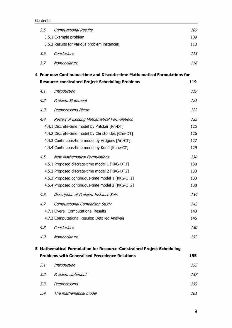
3.5 Computational Results 109
3.5.1 Example problem 109
3.5.2 Results for various problem instances 113
3.6 Conclusions 115
3.7 Nomenclature 116
4 Four new Continuous-time and Discrete-time Mathematical Formulations for
Resource-constrained Project Scheduling Problems 119
4.1 Introduction 119
4.2 Problem Statement 121
4.3 Preprocessing Phase 122
4.4 Review of Existing Mathematical Formulations 125
4.4.1 Discrete-time model by Pritsker [Pri-DT] 125
4.4.2 Discrete-time model by Christofides [Chri-DT] 126
4.4.3 Continuous-time model by Artigues [Art-CT] 127
4.4.4 Continuous-time model by Koné [Kone-CT] 129
4.5 New Mathematical Formulations 130
4.5.1 Proposed discrete-time model 1 [KKG-DT1] 130
4.5.2 Proposed discrete-time model 2 [KKG-DT2] 133
4.5.3 Proposed continuous-time model 1 [KKG-CT1] 133
4.5.4 Proposed continuous-time model 2 [KKG-CT2] 138
4.6 Description of Problem Instance Sets 139
4.7 Computational Comparison Study 142
4.7.1 Overall Computational Results 143
4.7.2 Computational Results: Detailed Analysis 145
4.8 Conclusions 150
4.9 Nomenclature 152
5 Mathematical Formulation for Resource-Constrained Project Scheduling
Problems with Generalised Precedence Relations 155
5.1 Introduction 155
5.2 Problem statement 157
5.3 Preprocessing 159
5.4 The mathematical model 161

Contents
10
5.5 Computational Results 166
5.6 Description of Problem Sets 166
5.7 Computational Study Results 167
5.8 Conclusions 172
5.9 Nomenclature 173
6 Conclusions and future work 175
6.1 Conclusions 175
6.2 Future Work 177
7 Publications 179
8 References 181
List of Figures
11
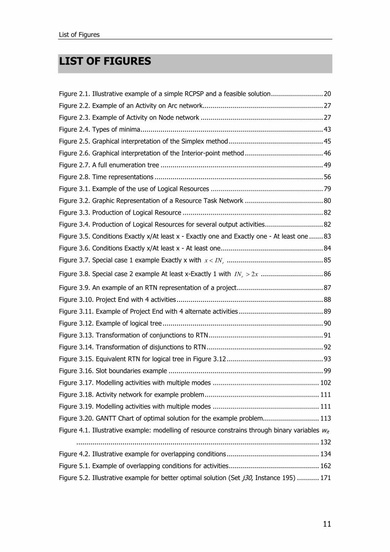
LIST OF FIGURES
Figure 2.1. Illustrative example of a simple RCPSP and a feasible solution .......................... 20
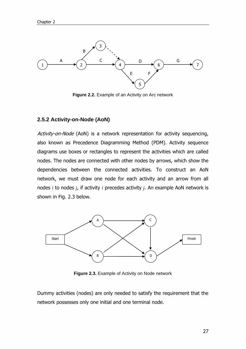
Figure 2.2. Example of an Activity on Arc network ............................................................ 27
Figure 2.3. Example of Activity on Node network ............................................................. 27
Figure 2.4. Types of minima ........................................................................................... 43
Figure 2.5. Graphical interpretation of the Simplex method ............................................... 45
Figure 2.6. Graphical interpretation of the Interior-point method ....................................... 46
Figure 2.7. A full enumeration tree ................................................................................. 49
Figure 2.8. Time representations .................................................................................... 56
Figure 3.1. Example of the use of Logical Resources ........................................................ 79
Figure 3.2. Graphic Representation of a Resource Task Network ....................................... 80
Figure 3.3. Production of Logical Resource ...................................................................... 82
Figure 3.4. Production of Logical Resources for several output activities ............................. 82
Figure 3.5. Conditions Exactly x/At least x - Exactly one and Exactly one - At least one ....... 83
Figure 3.6. Conditions Exactly x/At least x - At least one ................................................... 84
Figure 3.7. Special case 1 example Exactly x with rINx ................................................ 85
Figure 3.8. Special case 2 example At least x-Exactly 1 with xINr 2 ............................... 86
Figure 3.9. An example of an RTN representation of a project ........................................... 87
Figure 3.10. Project End with 4 activities ......................................................................... 88
Figure 3.11. Example of Project End with 4 alternate activities .......................................... 89
Figure 3.12. Example of logical tree ................................................................................ 90
Figure 3.13. Transformation of conjunctions to RTN ......................................................... 91
Figure 3.14. Transformation of disjunctions to RTN .......................................................... 92
Figure 3.15. Equivalent RTN for logical tree in Figure 3.12 ................................................ 93
Figure 3.16. Slot boundaries example ............................................................................. 99
Figure 3.17. Modelling activities with multiple modes ..................................................... 102
Figure 3.18. Activity network for example problem ......................................................... 111
Figure 3.19. Modelling activities with multiple modes ..................................................... 111
Figure 3.20. GANTT Chart of optimal solution for the example problem............................ 113
Figure 4.1. Illustrative example: modelling of resource constrains through binary variables wit
......................................................................................................................... 132
Figure 4.2. Illustrative example for overlapping conditions .............................................. 134
Figure 5.1. Example of overlapping conditions for activities ............................................. 162
Figure 5.2. Illustrative example for better optimal solution (Set j30, Instance 195) ........... 171
List of Tables
12
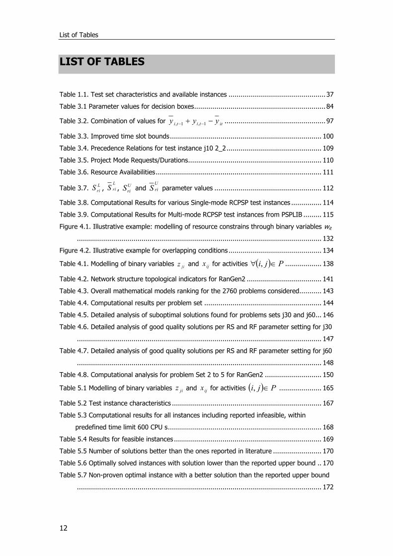
LIST OF TABLES
Table 1.1. Test set characteristics and available instances ................................................ 37
Table 3.1 Parameter values for decision boxes ................................................................. 84
Table 3.2. Combination of values for ittitiyyy 1,1, .................................................. 97
Table 3.3. Improved time slot bounds ........................................................................... 100
Table 3.4. Precedence Relations for test instance j10 2_2 ............................................... 109
Table 3.5. Project Mode Requests/Durations .................................................................. 110
Table 3.6. Resource Availabilities .................................................................................. 111
Table 3.7. L
riS , L
riS , U
riS and U
riS parameter values ..................................................... 112
Table 3.8. Computational Results for various Single-mode RCPSP test instances ............... 114
Table 3.9. Computational Results for Multi-mode RCPSP test instances from PSPLIB ......... 115
Figure 4.1. Illustrative example: modelling of resource constrains through binary variables wit
......................................................................................................................... 132
Figure 4.2. Illustrative example for overlapping conditions .............................................. 134
Table 4.1. Modelling of binary variables jiz and ijx for activities Pji , .................. 138
Table 4.2. Network structure topological indicators for RanGen2 ..................................... 141
Table 4.3. Overall mathematical models ranking for the 2760 problems considered ........... 143
Table 4.4. Computational results per problem set .......................................................... 144
Table 4.5. Detailed analysis of suboptimal solutions found for problems sets j30 and j60 ... 146
Table 4.6. Detailed analysis of good quality solutions per RS and RF parameter setting for j30
......................................................................................................................... 147
Table 4.7. Detailed analysis of good quality solutions per RS and RF parameter setting for j60
......................................................................................................................... 148
Table 4.8. Computational analysis for problem Set 2 to 5 for RanGen2 ............................ 150
Table 5.1 Modelling of binary variables jiz and ijx for activities Pji , ..................... 165
Table 5.2 Test instance characteristics .......................................................................... 167
Table 5.3 Computational results for all instances including reported infeasible, within
predefined time limit 600 CPU s ............................................................................ 168
Table 5.4 Results for feasible instances ......................................................................... 169
Table 5.5 Number of solutions better than the ones reported in literature ........................ 170
Table 5.6 Optimally solved instances with solution lower than the reported upper bound .. 170
Table 5.7 Non-proven optimal instance with a better solution than the reported upper bound
......................................................................................................................... 172

Chapter 1
13
Chapter 1
Introduction
1.1 Project Scheduling and Management
Project scheduling plays a vital role in project management, and constitutes
one of the most important directions in both research and practice in the
Operational Research (OR) field. The term project means different things to
different people and according to ISO 10006 (2003) Guideline for Quality in
Project Management (Section 3.5), it is used to describe a:
Unique process, consisting of a set of co-ordinated and controlled activities
with start and finish dates, undertaken to achieve an objective conforming to
specific requirements including constraints of time, cost and resources.
The same ISO, states some of the characteristics a project must have:
1. Unique, non-repetitive phases consisting of processes and
activities.
2. Expected to deliver specified (minimum) quality results within pre-
determined parameters.
3. Have planned start and finish dates, within clearly specified cost
and resource constraints.
A project is a one-time endeavour with a specific objective that must be
achieved, under cost, resource and time constraints. The relationships
between the various tasks that have to be performed to achieve the project’s
objectives can be very complex.
The process of project management involves three phases, planning,
scheduling and controlling. In the planning phase we define the activities that
Introduction
14
must be carried out to achieve the project objective and their characteristics
(i.e., duration, resource requirements, relationships, constraints, etc). During
the scheduling phase, the actual project schedule is produced, containing
activity starting and/or finishing times. Finally, the control phase focuses on
examining and determining solutions when variations from the original
schedule occur.
1.2 The Resource-Constrained Project Scheduling Problem
Quantitative approaches to project management date back to the 1950s.
Early solution procedures like the Critical Path Method (CPM) by Kelley and
Walker (1959) and Project Evaluation and Review Technique (PERT) by
Malcolm et al. (1959), only took into account activity durations (deterministic
or probabilistic) and assumed resources to be available in unlimited
quantities. However, in most practical situations this assumption is not
realistic, since the required resources are limited and to produce a functional
schedule the solution method should take them into account. The additional
constraints imposed by the limited resources, significantly increase the
problem hardness. According to Blazewicz et al. (1983) the Resource-
Constrained Project Scheduling Problem (RCPSP) belongs to the class of
strongly NP-hard problems.
During the last decades, the RCPSP has become a standard problem for
project scheduling in the OR literature. The RCPSP involves the construction
of a precedence and resource feasible time schedule which identifies the
starting and completion times of activities, under a specific objective. A
project consists of a set of interconnected activities and resources, logically
linked. These activities usually have to be performed for a successful project
completion. Several variations of the RCPSP exist that represent different
practical problems with different objectives, resource types, more than one
way (mode) to execute an activity, generalised precedence relations for
activities, e.t.c.
Chapter 1
15
1.3 Challenges and Motivation
OR uses scientific techniques and tools from various disciplines such as
informatics, mathematics, economics, chemistry, even biology to assist
decision making or provide a solution to a given problem (preferably optimal).
Over the years, the methodology of project scheduling has been developing
constantly, trying, from one side to model adequately new practical problems,
and, from the other side, to efficiently solve the resulting optimisation
problems. The methodology benefited from the development of both:
optimisation (especially combinatorial one) and computational possibilities.
A number of solution methods for the RCPSP, both exact and approximate
have been proposed in the OR literature. Exact techniques usually include
mathematical programming formulations and specialised branch-and-bound
algorithms. Due to the high degree of complexity of RCPSPs, an even larger
number of approximate methods such as heuristics and metaheuristics have
also been proposed. Roughly speaking, a heuristic is a technique designed to
solve a problem, or find an approximate solution with low computational
requirements, when classic methods fail to find any exact solution. By trading
optimality, completeness, accuracy, and/or precision for speed, a heuristic
can quickly produce a solution that is good enough for solving the problem at
hand.
Scheduling is a critical issue both in project management and process
operations. Process and project scheduling problems, share common features
such as required resource types, precedence relations and initial/target
inventories. The process scheduling problem consists of determining the most
efficient way to produce a set of products in a time horizon given a set of
processing recipes and limited resources. The activities to be scheduled
usually take place in multiproduct and multipurpose plants, in which a wide
variety of different products can be manufactured via the same recipe or
different recipes by sharing limited resources, such as equipment, material,
Introduction
16
time, and utilities. The common problem features, such as required resource
types, precedence relations and initial/target inventories, suggest that
exchanging solution techniques between the two research fields is both
possible and useful.
The process scheduling industry is driven by the substantial advances of
related modelling and solution techniques, as well as the rapidly growing
computational power. Mathematical programming, especially Mixed Integer
Linear Programming (MILP), because of its rigorousness, flexibility and
extensive modelling capability, has become one of the most widely explored
methods for process scheduling problems.
On the other hand, project scheduling research effort has mostly focused on
developing approximate solution techniques. However, recent project
scheduling research papers (Koné et al. 2011, Bianco and Caramia 2012a,
2012b and Rieck et al. 2012) show a renewed interest for mathematical
programming-based solution strategies. The study of exact methods, and
especially mathematical programming techniques, for solving the RCPSP is of
particular theoretical and practical interest. Indeed, mathematical
programming solvers are often the only software available to industrial
practitioners. Moreover, the best lower bounds ever found on broadly-studied
RCPSP test instances, were obtained by a hybrid method (Demassey et al.,
2005) involving constraint propagation and the MILP formulation of
Christofides et al. (1987). Also, a branch-and-cut method based on the latter
formulation was developed by Zhu et al. (2006), to solve the multimode
RCPSP and yielded very competitive results on benchmark problems.
Taking advantage of the continuous commercial software and hardware
advances, the size and difficulty of the combinatorial problems that can be
solved are constantly growing. The main objective of this thesis is to develop
new project scheduling techniques inspired by the process scheduling
literature, similar to the paper of Koné et al (2011), which is based on the
Chapter 1
17
work of Pinto and Grossmann on batch process problems (1995).
1.4 Thesis Structure
The rest of this thesis consists of a literature review and state-of-the-art,
three novel research chapters and finally some concluding remarks.
Chapter 2 is an introduction to state-of-the-art in RCPSP. We discuss the
resource constrained project scheduling problem, its components, variants
and network representation techniques. Afterwards, commonly used objective
functions and a classification scheme are described. We then present the test
instance sets available for benchmarking new solution techniques, followed
by a discussion of mathematical programming concepts, which is the main
optimisation method used in this thesis. Next a thorough literature review of
both exact and approximate solution techniques is presented. Finally, we
describe the commercial software used to solve RCPSP test problem instances
and measure the performance of the proposed solution procedures.
Chapter 3 presents new mixed-integer linear programming models for the
deterministic single- and multi-mode resource constrained project scheduling
problem with renewable and non-renewable resources. The modelling
approach relies on the Resource-Task Network (RTN) representation, a
network representation technique used in process scheduling problems,
based on continuous-time models. First, we propose new RTN-based network
representation methods, and then we efficiently transform them into
mathematical formulations including a set of constraints describing
precedence relations, different types of resources and multiple objectives.
Finally, the applicability of the proposed formulations is illustrated using
several example problems under the most commonly addressed objective, the
makespan minimization.
Introduction
18
Chapter 4 introduces two new binary integer programming discrete-time
models and two novel precedence-based mixed integer continuous-time
formulations for the solution of standard resource-constrained project
scheduling problems. The proposed discrete-time models are based on the
definition of binary variables that describe the processing state of every
activity between two consecutive time points, while the proposed continuous-
time models are based on the concept of overlapping of activities, and the
definition of a number of newly introduced sets. These four novel
mathematical formulations are compared with four representative literature
models using a total number of 2760 well-known open-accessed benchmark
problem instances involving 30 and 60 activities. A detailed computational
comparison study demonstrates the salient performance of the proposed
mathematical formulations, that feature the best overall performance.
Chapter 5 presents a new precedence-based continuous-time formulation for
a challenging extension of the standard single-mode resource-constrained
project scheduling problem that also considers minimum and maximum time
lags (RCPSP/max), under the objective of minimizing the project makespan.
The proposed linear mixed integer programming model is an extension of the
continuous-time formulations proposed in Chapter 4 and is used to conduct
an extensive computational study on a total of 2,250 well-known and open-
accessed benchmark problem instances from the literature. Various problem
sizes are considered in the test sets involving 10, 20, 30, 50 and 100
activities. Computational results illustrate the efficient performance of the
proposed mathematical formulation.
Finally, concluding remarks and future research directions are drawn in
Chapter 6.
Chapter 2
19
Chapter 2
State-of-the-Art
In this chapter we first discuss the resource constrained project scheduling
problem, its components, variants and network representation techniques.
Afterwards, commonly used objective functions and a classification scheme
are described. We then present the test instance sets available for
benchmarking new solution techniques, followed by a discussion of
mathematical programming concepts, which is the main optimisation method
used in this thesis. Next a thorough literature review of modelling and
solution techniques is presented. Finally, we describe the commercial
software used to solve RCPSP test problem instances and measure the
performance of the proposed solution procedures.
2.1 Resource-constrained project scheduling problem (RCPSP)
A project has a finite number of activities with specific durations. Precedence
relations between some activities are present and each activity requires
certain amounts of resources with limited availability, to be processed. For
modelling purposes, two dummy activities are added: (i) a start dummy
activity to represent the beginning of the project, and (ii) an end dummy
activity corresponding to the completion of the project. Dummy activities
have zero duration and zero resource requirements. The typical objective of
the RCPSP is to find an optimal (or at least feasible) schedule, while satisfying
time, precedence and resource constraints, such that a specific objective is
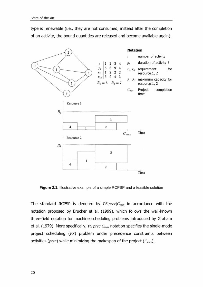
optimised (i.e., minimisation of the project makespan). An illustrative
example of a simple RCPSP and a feasible solution are displayed in Fig. 2.1.
In the standard RCPSP, all information data are deterministic. The resource
State-of-the-Art
20
type is renewable (i.e., they are not consumed, instead after the completion
of an activity, the bound quantities are released and become available again).
Notation
i number of activity
pi duration of activity i
ri1, ri2 requirement for
resource 1, 2
R1, R2 maximum capacity for
resource 1, 2
Cmax Project completion
time
Figure 2.1. Illustrative example of a simple RCPSP and a feasible solution
The standard RCPSP is denoted by PS|prec|Cmax in accordance with the
notation proposed by Brucker et al. (1999), which follows the well-known
three-field notation for machine scheduling problems introduced by Graham
et al. (1979). More specifically, PS|prec|Cmax notation specifies the single-mode
project scheduling (PS) problem under precedence constraints between
activities (prec) while minimizing the makespan of the project (Cmax).
Chapter 2
21
2.2 Project Activities
A project consists of activities, also known as jobs, operations, or tasks. In
order to complete the project successfully, all or some of the activities have
to be performed. Project activities have various characteristics, depending on
the tasks involved.
In some projects the processing of activities may be preempted (interrupted)
and recommenced at a later time (preempt-resume). In other cases, stopping
an activity is allowed, but resuming is not and it has to be restarted
(preempt-repeat). Finally, for certain activities preemption is not allowed at
all and once execution has started, it must be carried out to completion.
Another characteristic regards the order and timing in which activities are
executed. These precedence relations encountered in project scheduling
problems are presented in detail in the following section.
Activity ready times may need to be taken into account, durations can be
integer or continuous and deadlines may be imposed on each one or the
maximal project duration. The resource consumption can occur in constant or
variable amounts over their periods of execution.
Most problems assume a single execution mode per activity, while others
assume time/cost, time/resource and/or resource/resource trade-offs and
give rise to various possible execution modes. While the classical RCPSP is a
popular model, it cannot cover all situations that occur in practice. Therefore,
many researchers have developed more general project scheduling problems,
often using the standard RCPSP as a starting point. Such an example is the
Multi-mode Resource-Constrained Project Scheduling Problem (MRCPSP) or
MPS|prec|Cmax according to the notation of Brucker et al. (1999). In this
problem, the mode determines the duration of the activity and the
requirements for resources of various categories. Another extension studied

State-of-the-Art
22
by Salewski et al. (1997) are project scheduling problems which generalize
multiple activity modes to so-called mode identity constraints in which the set
of activities is partitioned into disjoint subsets. All activities in a subset must
then be executed in the same mode. Both the time and cost incurred by
processing a subset of activities depend on the resources assigned to it.
Finally, activities may require changeover times. When these times are
sequence-independent, we can include them in the activity durations.
However, sometimes changeovers are sequence-dependent (e.g. equipping
an excavator with different scoops and workers travelling between sites) and
must be taken into account separately in project settings.
2.3 Precedence Relations
Project activities are usually subject to precedence relations. In the rare case
where project activities can be performed in any order, no sophisticated
project scheduling solution procedures are required.
The traditional PERT/CPM methodology uses finish-start (FS) precedence
relations with zero time-lag, that is an activity can only start as soon as all its
predecessor activities have finished.
Precedence relations with zero time-lag between two activities are not always
enough. Elmaghraby and Kamburowski (1992) defined four types of
Generalized Precedence Relations (GPR): start-start (SS), start-finish (SF),
finish-start (FS) and finish-finish (FF) to model minimum and maximum time-
lags.
The minimal time-lag ( xSSijmin , xSFij
min , xFFijmin , xFSij
min ) specifies that
activity j can only start/finish when its predecessor i has already
started/finished for a certain time period (x time units). A maximal time-lag
Chapter 2
23
( xSSijmax , xSFij
max , xFFijmax , xFS ij
max ) specifies that activity j should be
started/finished at the latest x time periods after the start/finish of activity i.
In the minimal Finish-Start relation 0min
ijFS , an activity j (for example the
installation of a crane on a site) can start immediately after activity i (for
example the preparation of the site) has been finished. This strict finish-start
relation is the traditional PERT/CPM precedence relation mentioned before. If
a certain number of time units must elapse between the end of activity i and
the start of activity j (to allow for a lead time for example), the finish-start
relation receives a positive lead-lag factor. As such, 6min
ijFS means that the
start of activity j cannot be sooner than 6 time units after activity i finishes.
Minimal Start-Start relations denote that a certain time-lag must occur
between the start of two activities. The relationship 2min
ijSS for example,
denotes that the start of activity j (for example place pipe) must lag 2 time
units behind the start of activity i (level ground). 0min
ijSS denotes that
activity j (levelling concrete) can start as soon as activity i (pouring concrete)
has started. Ready time for activity i can be modelled by imposing a minimal
start-start relation between the start node in the project network and activity
i.
Minimal Finish-Finish relations are used quite often. xFFijmin represents the
requirement that the finish of an activity j (for example finish walls) must lag
the finish of activity i (for example install electricity) by x time units.
Start-finish relations occur very rarely in practice.
Combinations of the various types of generalized precedence relations can be
used. Consider the example of activity i (erect wall frames) and activity j
(install electricity). Both activities have a xSSijmin relationship (the
State-of-the-Art
24
electricians can only start installing electricity when sufficient wall frame
surface is in place), but since the electricians need some time to cope with
the output of the carpenters who are responsible for erecting the walls, both
activities also have a xFFijmin relation.
Maximal time-lags respectively impose a maximum number of time units
between the start/finish times of activities. An interesting usage of such time-
lags is a xSFijmax between the first and last activity in the project, which in
effect sets an upper bound to the project completion time.
The various types of GPRs can be represented in a standardized form by
reducing them to minimum SS precedence relationships, through the
transformations proposed by Bartusch et al. (1988). This extension of the
RCPSP is denoted as RCPSP/max or PS | temp | Cmax, using the notation of
Brucker et al. (1999). More specifically, PS | temp | Cmax notation specifies the
single-mode project scheduling problem (PS) under general temporal
constraints given by minimum and maximum start-start time lags between
activities (temp) while minimizing the makespan of the project (Cmax).
2.4 Resource Types
Each project activity (besides dummy ones) requires some resources for its
processing, that are available in limited amounts. Examples of resources are
raw materials, intermediate products, tools, machinery, manpower, financial,
energy, etc. Węglarz (1979) and Blazewicz et al. (1983) categorize resources
used by project activities as renewable, non-renewable and doubly
constrained.
Renewable resources are periodically renewed, but their quantity is limited
over each time period and may differ from one period to the next. Some
examples are manpower, machines, equipment, power and fuel flow.
Chapter 2
25
For non-renewable resources, constraints on availability only concern total
consumption over the whole period of project duration and not each time
period. Raw materials are a typical example of non-renewable resources,
since they are available at a specific quantity for a project.
Doubly constrained resource quantities are both per period and per project
constrained. Money is an example of such resource, since there is usually a
specific total budget for the entire project, as well as a limited cash flow per
period, according to progress. As formally shown by Talbot (1982), each
doubly constrained resource can be represented by one renewable and one
non-renewable resource, respectively.
Partially (non)renewable resources, introduced by Böttcher et al. (1996),
Schirmer and Drexl (1996) and Drexl (1997) limit utilization of resources
within a subset of the planning horizon. Essentially, partially (non)renewable
resources can be viewed as a generic resource concept in project scheduling,
as they include both renewable and non-renewable (and, hence doubly
constrained) resources. An example is that of a planning horizon of a month
with workers whose weekly working time, not the daily time, is limited by
their working contract.
It has been shown by Böttcher et al. (1999) both renewable and non-
renewable resource categories can be depicted by partially renewable
resources. A partially renewable resource, with a specified availability for a
time interval equal to a unit duration period, is essentially a renewable
resource. A partially renewable resource, with a specified availability for a
time interval equal to the project horizon, is essentially a non-renewable
resource. Partially renewable resources with a specified availability on both a
unit duration period and a total project horizon basis can be interpreted as
doubly constrained resources.
State-of-the-Art
26
2.5 Project Network Representations
Two representations have been commonly used to capture project networks,
the Activity-on-Arc (AoA) which is event-based and Activity-on-Node (AoN)
which is activity based. The latter represents activity interdependencies in a
more natural way, without the need for dummy activities. Understanding an
AoN is easier, even for inexperienced users. Finally, reviewing an AoN is
easier when a change occurs in the network.
2.5.1 Activity-on-Arc (AoA)
An Activity-on-Arc (AoA) diagram is based on the idea that each activity is a
transition between two events, its start and its end. Each activity is
represented as an arc, which starts and finishes at a node (drawn as a circle).
Each node represents an event, a point of zero time duration, which signifies
the completion of all the activities leading into it and the start of all activities
pointing out.
An AoA network can contain no cycles, because if it did, the transitivity
property of precedence would lead to the conclusion that an activity would
have to precede itself, which is impossible.
In AoA networks we use two dummy nodes to represent the start and
completion of the project. The initial event is the starting node of all activities
and has no predecessor(s), while the terminal event is the ending node of all
activities and has no successor(s).
Any two nodes may be connected by only one activity. So, for several
activities to be executed simultaneously, we need to introduce dummy
activities. Dummy activities are drawn as dotted arcs, consume no resources
and have zero time duration. An example of an AoA diagram is shown in Fig.
2.2 below.
Chapter 2
27
Figure 2.2. Example of an Activity on Arc network
2.5.2 Activity-on-Node (AoN)
Activity-on-Node (AoN) is a network representation for activity sequencing,
also known as Precedence Diagramming Method (PDM). Activity sequence
diagrams use boxes or rectangles to represent the activities which are called
nodes. The nodes are connected with other nodes by arrows, which show the
dependencies between the connected activities. To construct an AoN
network, we must draw one node for each activity and an arrow from all
nodes i to nodes j, if activity i precedes activity j. An example AoN network is
shown in Fig. 2.3 below.
Figure 2.3. Example of Activity on Node network
Dummy activities (nodes) are only needed to satisfy the requirement that the
network possesses only one initial and one terminal node.
A
B
C
Start Finish
D
1 2 4 6 7
3
5
A
B
C
E F
D G

State-of-the-Art
28
The AoN has certain advantages over the AoA, since it represents activity
interdependencies in a more natural way, it is easier to understand, even for
inexperienced users, and easier to review when a change occurs in the
network. A more thorough comparison of the two methods can be found in
Kolisch and Padman (2001).
2.6 Objectives of Project Scheduling
Project scheduling objective functions can be can be regular or non-regular. A
regular performance measure is a non-decreasing function of the activity
completion times (in the case of a minimization problem), otherwise it is non-
regular. Regular objective functions have received much more attention in the
literature than non-regular ones, especially the make span or project length.
Each of the objectives for deterministic project scheduling, presented in the
following sections can and has been examined for problems with a diversity
of resource and activity characteristics.
2.6.1 Time-based objectives
Minimizing the project make span is undoubtedly the most popular time-
based objective function discussed in the project scheduling literature. Most
often it is recognized as the most relevant objective in various review papers,
Kolisch (1996b), Herroelen (2005), Hartmann et al. (2010). According to
Kolisch (1996b):
1. The majority of income payments of projects (e.g. in the
construction industry) occur at the end of a project or at the end of
predefined project phases. Finishing the project early reduces the
amount of tied-up capital.
2. The quality of forecasts tends to deteriorate with the distance into
the future of the period for which they are made. Minimizing the
Chapter 2
29
project duration reduces the planning horizon and, therefore, the
uncertainty of data.
3. Finishing products as early as possible lowers the probability of
time-overruns of the project.
4. By freeing resource capacity as early as possible the flexibility of
the company can be raised in order to better cope with changes of
the economic environment.
5. Additionally, high resource utilization at the beginning of the
planning horizon leads to a larger amount of free resources at the
end of the planning horizon and, thus, raises the ability to accept
and process new projects.
Other time-based objectives based on project lateness, tardiness and
earliness exist. The lateness iL of an activity i is the difference of its
completion time and its due date. The lateness can be zero (if the task
finishes on time), positive (if the task finishes later) or negative (if the task
finishes earlier). The tardiness iT is the same as lateness, but it cannot be
negative ( max 0,i iT L ). Earliness iE is defined as max 0,i iE L .
In the literature, we encounter a number of objectives based on lateness,
tardiness and earliness, such as minimization of the weighted tardiness
(Kolisch, 2000), minimization of the maximum lateness and of the weighted
total tardiness (Neumann, 2002), etc.
2.6.2 Maximizing the Net Present Value
The value of a certain amount of money is a function of the time of receipt or
disbursement of the cash. Money received today is more valuable than money
to be received in some future time period, because it can be invested to start
earning interest immediately. The nature and timing of the cash flows in
projects depend on the contract. The contractor would like to receive as
State-of-the-Art
30
much as possible, as early as possible to initiate activities, while the client
would like to delay payments for completion of parts of the project as long as
possible, since progress payments represent expenses.
To cope with such problems we need to set financial objectives related to
incoming and outgoing cash flows, including discount rates. Such objectives
are referred in literature as Maximizing the Net Present Value (NPV) of the
project and were introduced by Russell (1970).
In the unconstrained case, both the amount and timing of cash flows are
known and we attempt to maximize their NPV. Cash flows can be associated
with the completion of set of activities, occur at regular intervals (e.g.
weekly) or compounded to a single cash flow at the beginning/end of an
activity.
When both the amount and timing of the cash flows must be determined, we
have the payment scheduling problem. Finally, the resource-constrained case
is more complex, since we need to additionally deal with limited resources.
2.6.3 Other objectives
A number of other objectives has been examined in the literature, such as
minimizing resource availability costs (Demeulemeester 1995, Franck and
Schwindt 1995, Kimms 1998, Möhring 1984, Zimmermann 1997), the discrete
time/resource trade-off problem (Elmaghraby, 1977), minimizing the sum of
costs (Möhring et al. 2003, Achuthan and Hardjawidjaja, 2001), etc.
Finally, certain problems deal with multi-objective scheduling that requires
the optimisation of more than one objective (Nabrzyski and Węglarz 1994, Al-
Fawzana and Haouari 2005, Bomsdorf and Derigs 2008).
Chapter 2
31
2.7 A Classification Scheme
The increasing research interest in the area of Project Scheduling from both
science and practice has led to an ever growing number of problem types.
Various acronyms, such as RCPSP, MRCPSP, RCPSP-GPR have been
extensively used to describe the problem class. However, these abbreviations
offer an inadequate description of the problem characteristics and may often
lead to misconceptions.
Herroelen et al. (1998) proposed a classification system compatible with what
is generally accepted in machine scheduling (Graham et al., 1979) and
resource-constrained machine scheduling (Blazewicz et al., 1983), because
machine scheduling models are special cases of project scheduling models.
The proposed scheme resembles machine scheduling problems in that it is
also composed of three fields α | β | γ, but the composition of the fields and
the precise meaning of the various parameters are mostly new and specific to
the area of project scheduling. The meaning of each field is described below:
1. Field α – Represents resource characteristics and contains up
to three elements,
2. Field β – Represents activity characteristics and contains up to
nine fields and
3. Field γ – Contains one element and represents the
performance measures.
Brucker et al. (1999) provided their own classification scheme, but Herroelen
et al. (2000) revealed serious shortcomings and turned their own original
scheme into a unified classification scheme for resource scheduling
(Demeulemeester and Herroelen, 2002).
In the next sections, we cover the characteristic values of the three fields in
the original classification scheme (Herroelen, 1998) that apply to
deterministic project scheduling problems.
State-of-the-Art
32
2.7.1 Field α – Resource Characteristics
Field α, is a set describing the resource characteristics and consists of at most
three elements 1 , 2 and 3 . The symbol denotes an empty field and will
be used when a field is omitted.
Parameter m,1,1 represents the number of resource types used in the
problem:
1 no resource types are considered in the scheduling
problem
11 one resource type is considered
m1 the number of resource types is equal to m
The second parameter, 2 , describes the resource types used. As mentioned
in Section 2.4, in the project scheduling literature a common distinction is
made between various types of resources:
2 absence of any resource type specification
12 renewable resources, the availability of which is
specified for the unit duration period
T2 non-renewable resources, the availability of which
is specified for the entire project horizon T
T12 both renewable and nonrenewable resources
(including also doubly constrained resources, the
availability of which is specified on both a unit
duration period and a total project horizon basis)
v2 partially (non-)renewable resources the availability
of which is renewed in specific time periods
Chapter 2
33
Finally, parameter 3 describes the resource availability characteristics of the
problem.
3 (partially) renewable resources are available in
constant amounts
v3 (partially) renewable resources are available in
variable amounts
2.7.2 Field β – Activity Characteristics
The second field describes the activity characteristics of the problem, using
nine parameters. The first parameter 1 indicates the possibility of activity
preemption:
1 no activity preemption is allowed
pmtn1 Activity preemption of type preempt-resume is
allowed
reppmtn1 Activity preemption of type preempt-repeat is
allowed
Parameter 2 describes the activity precedence relations:
2 no precedence constraints exist (activities can be
executed at any order)
cpm2 only Finish-to-Start relationships with zero time lag
are used, as in the PERT/CPM model
min2 precedence diagramming relations with minimal
time lags are used
gpr2 the activities are subject to generalized precedence
relationships with minimal and maximal time lags
State-of-the-Art
34
The third parameter 3 , denotes the ready times for activities:
3 all ready times are zero
j 3 ready times vary per activity
Parameter 4 describes the duration of project activities:
4 arbitrary integer durations
cont4 arbitrary continuous durations
)(4 dd j all activities have a duration equal to d units
The fifth parameter 5 describes the project deadlines:
5 no deadlines
jd5 deadlines are imposed on individual project
activities
n 5 a deadline is imposed on the project
The next parameter 6 expresses the nature of resource requirements for
project activities:
6 constant discrete resource requirements (e.g. a
number of units for every time period of activity
execution)
vr6 variable discrete resource requirements (e.g. a
number of units which varies over the periods of
activity execution)
Chapter 2
35
If the activity durations have to be determined by the solution procedure on
the basis of a resource requirement function, then the following settings are
used:
disc6 The resource requirements are a discrete function
of the activity duration
cont6 The resource requirements are a continuous
function of the activity duration
int6 the activity resource requirements are expressed as
an intensity or rate function
If needed, the user can be more specific on the type of resource requirement
function (e.g. concave, convex, linear, e.t.c.)
The type and number of possible execution modes of project activities is
described by parameter 7 .
7 activities are performed in a single execution mode
mu7 activities have multiple preset execution modes
id7 Activities are subject to mode identity constraints
The next parameter 8 is used to address financial issues of the project
activities. Most models with cash flows, assume the cash flow amounts to be
known. Other models assume that the cash flows are periodic in that they
occur at regular time intervals or with a known frequency. Still other models
assume that both the amount and the timing of the cash flows have to be
determined.
8 no cash flows are specified
jc8 activities have associated cash flows
State-of-the-Art
36
jc8 activities have an associated positive cash flow
per8 periodic cash flows are specified
sched8 both the amount and timing of the cash flows have
to be determined
Finally parameter 9 denotes the changeover times. Changeover times are
usually sequence-independent, so we include them in the activity durations.
However, sometimes changeovers are sequence-dependent (e.g. equipping
an excavator with different scoops and workers travelling between sites) and
must be taken into account in project settings:
9 no changeover times
jks9 Sequence-dependent changeover times
2.7.3 Field γ – Performance Measures
The last field is used to define the performance measures:
reg the performance measure is any regular measure
nonreg the performance measure is any nonregular
measure
Obviously, the list of performance measures is practically endless. Some
examples of such measures are:
maxC minimize the project makespan
npv maximize the net present value of the project
F minimize the average flow time over all subprojects
or activities
curve determine the time vs cost trade-off curve
Chapter 2
37
rac minimize the resource availability costs
maxL minimize the project lateness
maxT minimize the project tardiness
av minimize the resource allocations whilst meeting
the project deadlines
multi multiple objectives
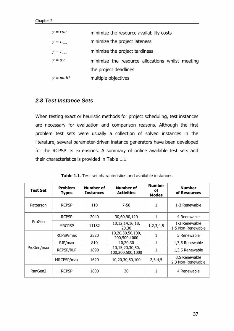
2.8 Test Instance Sets
When testing exact or heuristic methods for project scheduling, test instances
are necessary for evaluation and comparison reasons. Although the first
problem test sets were usually a collection of solved instances in the
literature, several parameter-driven instance generators have been developed
for the RCPSP its extensions. A summary of online available test sets and
their characteristics is provided in Table 1.1.
Table 1.1. Test set characteristics and available instances
Test Set Problem
Types Number of Instances
Number of Activities
Number of
Modes
Number of Resources
Patterson RCPSP 110 7-50 1 1-3 Renewable
ProGen
RCPSP 2040 30,60,90,120 1 4 Renewable
MRCPSP 11182 10,12,14,16,18,
20,30 1,2,3,4,5
1-3 Renewable 1-5 Non-Renewable
ProGen/max
RCPSP/max 2520 10,20,30,50,100,
200,500,1000 1 5 Renewable
RIP/max 810 10,20,30 1 1,3,5 Renewable
RCPSP/RLP 1890 10,15,20,30,50,
100,200,500,1000 1 1,3,5 Renewable
MRCPSP/max 1620 10,20,30,50,100 2,3,4,5 3,5 Renewable
2,3 Non-Renewable
RanGen2 RCPSP 1800 30 1 4 Renewable
State-of-the-Art
38
2.8.1 Patterson test set
Patterson (1984) was the first to assemble a set of 110 test problems (with 7
up to 50 activities and 1 to 3 renewable resource types) which over the years
became a standard for validating optimal and suboptimal procedures for the
RCPSP. But Herroellen et al. (1998) pointed out that test sets should span the
full range of complexity, from very easy to very hard problem instances
generated by using a controlled design of specified problem parameters. The
generation of easy and hard problem instances, however, appears to be a
very difficult task which heavily depends on the possibility to isolate the
factors that precisely determine the computing effort required by the solution
procedure used to solve a problem, and the calibration of the scale that
characterizes such effort. Such problem sets are generated by ProGen
proposed by Kolisch et al. (1995) that quickly replaced the Patterson test
problem set.
2.8.2 ProGen and ProGen/max
ProGen was developed by Kolisch et al. (1995), as a network instance
generator for the classical RCPSP as well as the multi-mode extension. A
number of instances, systematically generated by ProGen, are available for
researchers in PSPLIB (Kolisch and Sprecher, 1996), an online scheduling
library (http://129.187.106.231/psplib/). PSPLIB test sets have been used as
a benchmark in a large number of studies. According to the review papers by
Herroelen (2005), Lancaster and Ozbayrak (2007) and Hartmann and
Briskorn (2010), it is the most widely used test bed for the RCPSP and its
variations.
The library contains data sets that can be used for the evaluation of solution
procedures for single- and multi-mode resource-constrained project
scheduling problems, as well as reported optimal and heuristic solutions.
Researchers can download the benchmark sets to evaluate their algorithms,
Chapter 2
39
and send their results to be added to the library, or generate their own test-
data.
Schwindt (1996) developed a version called ProGen/max in order to include
minimal and maximal time lags. This generator can also produce activities
with multiple modes as well as instances for the resource levelling and the
resource investment problem.
2.8.3 RanGen and RanGen2
The generators presented in the previous sections do not generate strongly
random networks because they do not allow selection from the full space of
feasible networks. Hence, Demeulemeester et al. (2003) developed RanGen,
which claims to generate strongly random networks that conform to desired
values of complexity measures. RanGen produces single- and multi-mode
project instances based on different control parameters than ProGen.
Vanhoucke et al. (2008) enhanced RanGen to RanGen2, by incorporating
further topological network measures.
2.8.4 Other test instance generators
A test set generator for AOA project networks was proposed by Agrawal et al.
(1996). In this generator, named DAGEN, the user can specify the level of a
summary measure of network complexity. Browning and Yassine (2010)
presented a generator for problems consisting of multiple projects with
controlled resource distributions and amounts of resource contention. They
also generated 12,320 test problems for a full-factorial experiment and used
analysis of means to conclude that the generator produces “near-strongly
random” problems.
State-of-the-Art
40
2.9 Mathematical Programming
Mathematical Programming is the use of mathematical models, particularly
optimising models, to assist in taking decisions. It is very different and should
not be confused with computer programming, even though solving most
practical problems requires the use of computer calculating power.
The term programming is actually used in the sense of planning/scheduling.
The goal of mathematical programming is to optimise (minimise or maximise)
a quantity. This quantity is known as the objective function.
2.9.1 Mathematical Modelling
Many scientific applications utilise models as a structure to present features
and characteristics of an “object”. Sometimes models are physical, such as a
model aircraft used in wind tunnels to test its aerodynamics. However, the
models examined in operational research are abstract. These abstract models
are usually mathematical and involve a set of mathematical relationships
involving equations, inequalities and logical dependencies to describe real-
world relationships and constraints.
Building a mathematical model gives us greater insight and understanding of
the “object” being modelled. A number of not so obvious aspects are revealed
and further mathematical analysis can lead to different courses of action.
Finally, it is easier to implement various “scenarios”, however radical, and
harmlessly observe their outcome.
It is important to understand that a model is actually defined by its
relationships and constraints. These are, to a large extent, independent of the
data in the model. This means that a model can be used in a variety of
similar situations, that differ in the data involved (i.e., costs, resource
availabilities, activity durations, etc).
Chapter 2
41
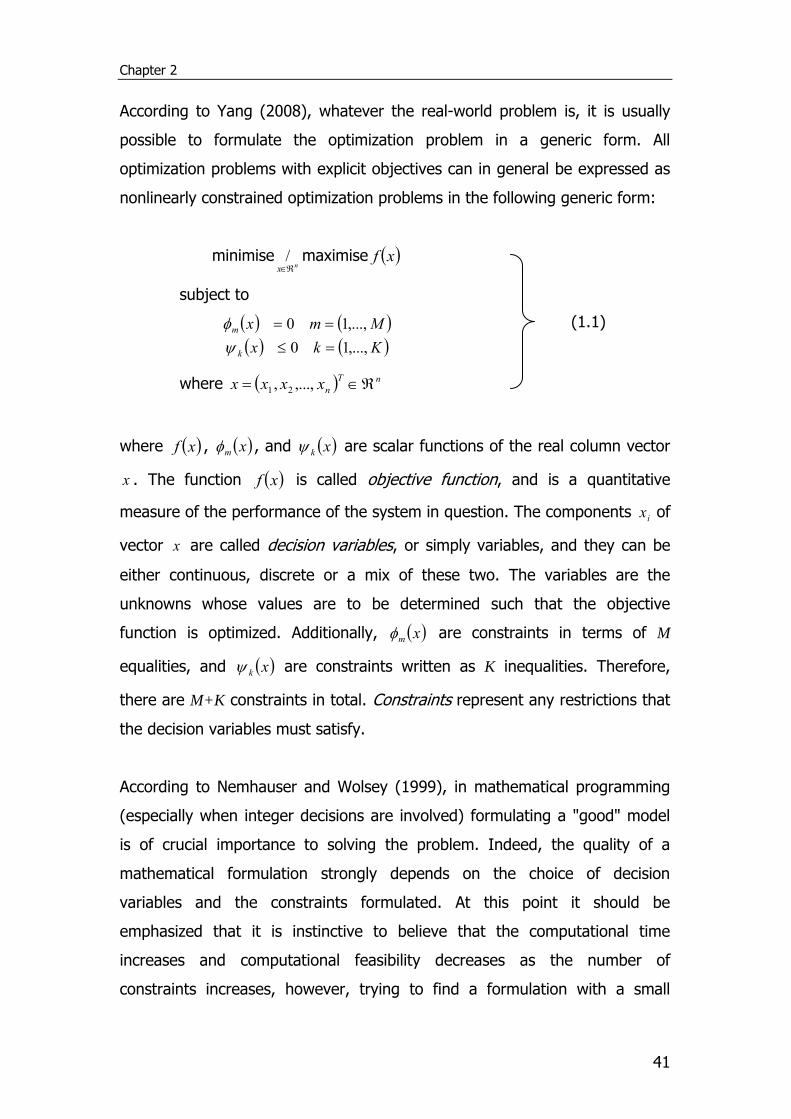
According to Yang (2008), whatever the real-world problem is, it is usually
possible to formulate the optimization problem in a generic form. All
optimization problems with explicit objectives can in general be expressed as
nonlinearly constrained optimization problems in the following generic form:
minimisenx / maximise xf
subject to
Kkx
Mmx
k
m
,...,10
,...,10
where nT
nxxxx ,...,, 21
(1.1)
where xf , xm , and xk are scalar functions of the real column vector
x . The function xf is called objective function, and is a quantitative
measure of the performance of the system in question. The components ix of
vector x are called decision variables, or simply variables, and they can be
either continuous, discrete or a mix of these two. The variables are the
unknowns whose values are to be determined such that the objective
function is optimized. Additionally, xm are constraints in terms of M
equalities, and xk are constraints written as K inequalities. Therefore,
there are M+K constraints in total. Constraints represent any restrictions that
the decision variables must satisfy.
According to Nemhauser and Wolsey (1999), in mathematical programming
(especially when integer decisions are involved) formulating a "good" model
is of crucial importance to solving the problem. Indeed, the quality of a
mathematical formulation strongly depends on the choice of decision
variables and the constraints formulated. At this point it should be
emphasized that it is instinctive to believe that the computational time
increases and computational feasibility decreases as the number of
constraints increases, however, trying to find a formulation with a small
State-of-the-Art
42
number of constraints is often a very bad strategy (Nemhauser and Wolsey,
1999).
The procedure of identifying the decision variables, constraints and objective
function is known as modelling. Depending on the properties of the functions
f , , and and the vector x , the mathematical program (1.1) is called:
Linear: If x is continuous and the functions f , , and are all
linear.
Nonlinear: If x is continuous and at least one of the functions f , ,
and is nonlinear.
Mixed integer linear: If x requires at least some of the variables ix to
take integer (or binary) values only; and the functions f , , and
are linear.
Mixed integer nonlinear: If x requires at least some of the variables ix
to take integer (or binary) values only; and at least one of the
functions f , , and is nonlinear.
2.9.2 Types of optimal solutions
The feasible region contains the set of feasible solutions to the problem,
0,0| xxxF km
n . A feasible solution *x that optimises the
objective function is called optimal, FxxforxfFx ,: ** . The
value of the objective function for the optimal solution *xf should be less
or equal ( ) to every other value, with Fx , when we have a minimisation
problem and greater or equal ( ) for a maximisation problem.
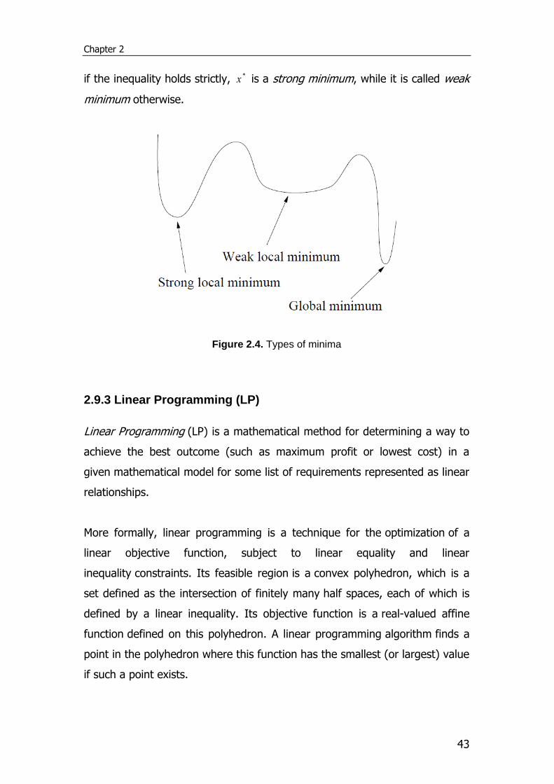
If for a minimisation problem, the property xfxf * is satisfied for all
Fx , then *x is a global minimum. If this condition is satisfied for all x in a
neighbourhood of *x , then it is a local minimum, as shown in Fig. 2.4. Finally,
Chapter 2
43
if the inequality holds strictly, *x is a strong minimum, while it is called weak
minimum otherwise.
Figure 2.4. Types of minima
2.9.3 Linear Programming (LP)
Linear Programming (LP) is a mathematical method for determining a way to
achieve the best outcome (such as maximum profit or lowest cost) in a
given mathematical model for some list of requirements represented as linear
relationships.
More formally, linear programming is a technique for the optimization of a
linear objective function, subject to linear equality and linear
inequality constraints. Its feasible region is a convex polyhedron, which is a
set defined as the intersection of finitely many half spaces, each of which is
defined by a linear inequality. Its objective function is a real-valued affine
function defined on this polyhedron. A linear programming algorithm finds a
point in the polyhedron where this function has the smallest (or largest) value
if such a point exists.
State-of-the-Art
44
Linear programs are problems that can be expressed in canonical form:
maximise xcT
subject to bAx
and 0x
(1.2)
where x represents the vector of variables (to be determined), c and b are
vectors of (known) coefficients, A is a (known) matrix of coefficients, and
T is the matrix transpose. The expression to be maximized or minimized is
called the objective function ( xcT in this case). The inequalities bAx are
the constraints which specify a convex polytope over which the objective
function is to be optimised. In this context, two vectors are comparable when
they have the same dimensions. If every entry in the first is less-than or
equal-to the corresponding entry in the second then we can say the first
vector is less-than or equal-to the second vector.
Two well-known solution procedures for LP problems are the Simplex
algorithm and the interior points method.
Simplex Algorithm
The Simplex Algorithm, developed by George Dantzig in 1947, solves LP
problems by starting with an initial Basic Feasible Solution (BFS) and testing
its optimality. If the optimality condition is verified, then the algorithm
terminates. Otherwise, the algorithm identifies an adjacent BFS, with a better
objective value. The optimality of this new solution is tested again, and the
entire scheme is repeated, until an optimal BFS is found. Since every time a
new BFS is identified the objective value is improved (except from a certain
pathological case that we shall see later), and the set of BFS’s is finite, it
follows that the algorithm will terminate in a finite number of steps
(iterations).
Chapter 2
45
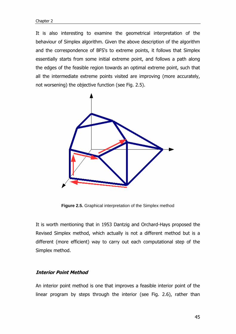
It is also interesting to examine the geometrical interpretation of the
behaviour of Simplex algorithm. Given the above description of the algorithm
and the correspondence of BFS's to extreme points, it follows that Simplex
essentially starts from some initial extreme point, and follows a path along
the edges of the feasible region towards an optimal extreme point, such that
all the intermediate extreme points visited are improving (more accurately,
not worsening) the objective function (see Fig. 2.5).
Figure 2.5. Graphical interpretation of the Simplex method
It is worth mentioning that in 1953 Dantzig and Orchard-Hays proposed the
Revised Simplex method, which actually is not a different method but is a
different (more efficient) way to carry out each computational step of the
Simplex method.
Interior Point Method
An interior point method is one that improves a feasible interior point of the
linear program by steps through the interior (see Fig. 2.6), rather than
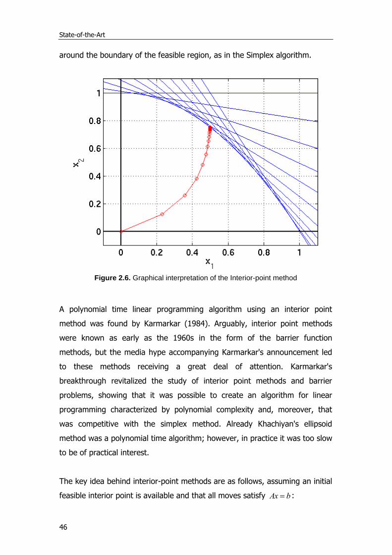
State-of-the-Art
46
around the boundary of the feasible region, as in the Simplex algorithm.
Figure 2.6. Graphical interpretation of the Interior-point method
A polynomial time linear programming algorithm using an interior point
method was found by Karmarkar (1984). Arguably, interior point methods
were known as early as the 1960s in the form of the barrier function
methods, but the media hype accompanying Karmarkar's announcement led
to these methods receiving a great deal of attention. Karmarkar's
breakthrough revitalized the study of interior point methods and barrier
problems, showing that it was possible to create an algorithm for linear
programming characterized by polynomial complexity and, moreover, that
was competitive with the simplex method. Already Khachiyan's ellipsoid
method was a polynomial time algorithm; however, in practice it was too slow
to be of practical interest.
The key idea behind interior-point methods are as follows, assuming an initial
feasible interior point is available and that all moves satisfy bAx :
Chapter 2
47
1. Try to move through the interior in directions that show promise of
moving quickly to the optimal solution.
2. Recognize that if we move in a direction that sets the new point too
"close" to the boundary, this will be an obstacle that will impede our
moving quickly to an optimal solution. One way around this is to
transform the feasible region so that the current feasible interior point
is at the center of the transformed feasible region. Once a movement
has been made, the new interior point is transformed back to the
original space, and the whole process is repeated with the new point
as the center.
3. The simple stopping rule typically followed is to stop with an
approximate optimal solution when the difference between iterates
"deemed" sufficiently small in the original space.
2.9.4 Mixed Integer Programming (MIP)
A Mixed-Integer Programming (MIP) problem results when some of the
variables in your model are real-valued and some of the variables are integer
and/or binary. The model is therefore “mixed”. Integer variables appear when
modelling indivisible entities, while a very common use of binary (0–1)
variables is to represent binary choice. Consider an event that may or may
not occur, and suppose that it is part of the problem to decide between these
possibilities. In order to model such a choice, a binary variable, which
typically equals 1 if the event occurs otherwise is set to zero, can be used.
Depending on the specific problem the event may represent yes/no decisions,
logical conditions, fixed costs or piecewise linear functions.
Mixed Integer Programming (MIP) problems can be expressed in standard
form, as follows:

State-of-the-Art
48
maximise hyxcT
subject to bGyAx
0x and
0y is integer or binary
(1.3)
where x represents the vector of non-negative variables, y represents the
vector of integer and/or binary variables, c and b are vectors of coefficients,
and A and G are matrices of coefficients. In this case the objective function
is hyxcT .
For further reading on MIP optimisation, we refer to the excellent books of
Floudas (1995) and Nemhauser and Wolsey (1999). MIP problems are usually
solved using branch-and-bound, cutting planes or branch-and-cut methods.
Branch-and-Bound Techniques
Branch and Bound (B&B) is by far the most widely used tool for solving large
scale NP-hard combinatorial optimization problems (Floudas, 1995). The
method was first proposed by Land and Doig (1960) for discrete
programming. The Branch and Bound technique consists of a systematic
enumeration of all candidate solutions, where large subsets of fruitless
candidates are discarded en masse, by using upper and lower estimated
bounds of the quantity being optimized.
The method is based on the observation that the enumeration of integer
solutions has a tree structure. For example, consider the complete
enumeration of a model having one general integer variable 1x , and two
binary variables 2x and 3x , whose ranges are 31 1 x , 10 2 x , and
10 3 x . Fig. 2.7 shows the complete enumeration of all of the solutions for
these variables, even those which might be infeasible due to other constraints
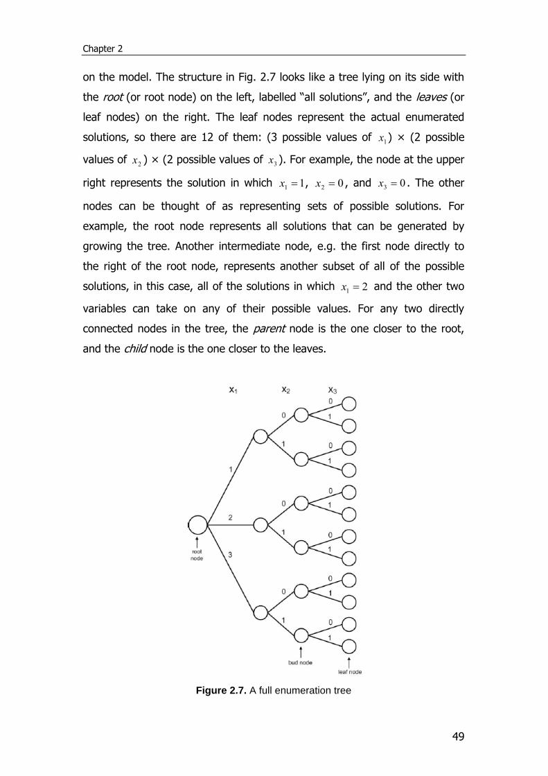
Chapter 2
49
on the model. The structure in Fig. 2.7 looks like a tree lying on its side with
the root (or root node) on the left, labelled “all solutions”, and the leaves (or
leaf nodes) on the right. The leaf nodes represent the actual enumerated
solutions, so there are 12 of them: (3 possible values of 1x ) × (2 possible
values of 2x ) × (2 possible values of 3x ). For example, the node at the upper
right represents the solution in which 11 x , 02 x , and 03 x . The other
nodes can be thought of as representing sets of possible solutions. For
example, the root node represents all solutions that can be generated by
growing the tree. Another intermediate node, e.g. the first node directly to
the right of the root node, represents another subset of all of the possible
solutions, in this case, all of the solutions in which 21 x and the other two
variables can take on any of their possible values. For any two directly
connected nodes in the tree, the parent node is the one closer to the root,
and the child node is the one closer to the leaves.
Figure 2.7. A full enumeration tree

State-of-the-Art
50
Now the main idea in branch and bound is to avoid growing the whole tree as
much as possible, because the entire tree is just too big in any real problem.
Instead branch and bound grows the tree in stages, and grows only the most
promising nodes at any stage. It determines which node is the most
promising by estimating a bound on the best value of the objective function
that can be obtained by growing that node to later stages. The name of the
method comes from the branching that happens when a node is selected for
further growth and the next generation of children of that node is created.
The bounding comes in when the bound on the best value attained by
growing a node is estimated. We hope that in the end we will have grown
only a very small fraction of the full enumeration tree.
Another important aspect of the method is pruning, in which you cut off and
permanently discard nodes when you can show that it, or any its
descendents, will never be either feasible or optimal. The name derives from
gardening, in which pruning means to clip off branches on a tree, exactly
what we will do in this case. Pruning is one of the most important aspects of
branch and bound since it is precisely what prevents the search tree from
growing too much.
To describe branch and bound in detail, we first need to introduce some
terminology:
Node: any partial or complete solution. For example, a node that is two
levels down in a 5-variable problem might represent the partial solution 3-
17-?-?-?, in which the first variable has a value of 3 and the second
variable has a value of 17. The values of the last three variables are not
yet set.
Leaf (leaf node): a complete solution in which all of the variable values
are known.
Bud (bud node): a partial solution, either feasible or infeasible. Think of
it as a node that might yet grow further, just as on a real tree.
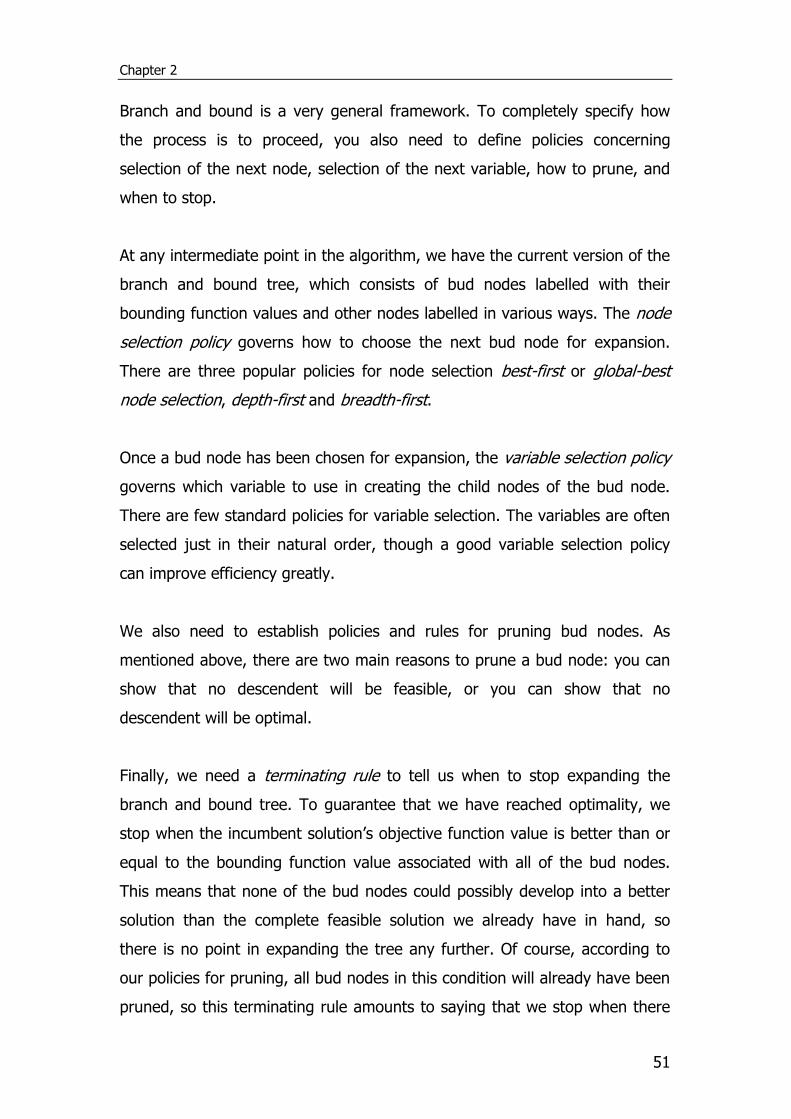
Chapter 2
51
Branch and bound is a very general framework. To completely specify how
the process is to proceed, you also need to define policies concerning
selection of the next node, selection of the next variable, how to prune, and
when to stop.
At any intermediate point in the algorithm, we have the current version of the
branch and bound tree, which consists of bud nodes labelled with their
bounding function values and other nodes labelled in various ways. The node
selection policy governs how to choose the next bud node for expansion.
There are three popular policies for node selection best-first or global-best
node selection, depth-first and breadth-first.
Once a bud node has been chosen for expansion, the variable selection policy
governs which variable to use in creating the child nodes of the bud node.
There are few standard policies for variable selection. The variables are often
selected just in their natural order, though a good variable selection policy
can improve efficiency greatly.
We also need to establish policies and rules for pruning bud nodes. As
mentioned above, there are two main reasons to prune a bud node: you can
show that no descendent will be feasible, or you can show that no
descendent will be optimal.
Finally, we need a terminating rule to tell us when to stop expanding the
branch and bound tree. To guarantee that we have reached optimality, we
stop when the incumbent solution’s objective function value is better than or
equal to the bounding function value associated with all of the bud nodes.
This means that none of the bud nodes could possibly develop into a better
solution than the complete feasible solution we already have in hand, so
there is no point in expanding the tree any further. Of course, according to
our policies for pruning, all bud nodes in this condition will already have been
pruned, so this terminating rule amounts to saying that we stop when there
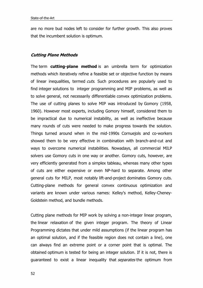
State-of-the-Art
52
are no more bud nodes left to consider for further growth. This also proves
that the incumbent solution is optimum.
Cutting Plane Methods
The term cutting-plane method is an umbrella term for optimization
methods which iteratively refine a feasible set or objective function by means
of linear inequalities, termed cuts. Such procedures are popularly used to
find integer solutions to integer programming and MIP problems, as well as
to solve general, not necessarily differentiable convex optimization problems.
The use of cutting planes to solve MIP was introduced by Gomory (1958,
1960). However most experts, including Gomory himself, considered them to
be impractical due to numerical instability, as well as ineffective because
many rounds of cuts were needed to make progress towards the solution.
Things turned around when in the mid-1990s Cornuejols and co-workers
showed them to be very effective in combination with branch-and-cut and
ways to overcome numerical instabilities. Nowadays, all commercial MILP
solvers use Gomory cuts in one way or another. Gomory cuts, however, are
very efficiently generated from a simplex tableau, whereas many other types
of cuts are either expensive or even NP-hard to separate. Among other
general cuts for MILP, most notably lift-and-project dominates Gomory cuts.
Cutting-plane methods for general convex continuous optimization and
variants are known under various names: Kelley's method, Kelley-Cheney-
Goldstein method, and bundle methods.
Cutting plane methods for MIP work by solving a non-integer linear program,
the linear relaxation of the given integer program. The theory of Linear
Programming dictates that under mild assumptions (if the linear program has
an optimal solution, and if the feasible region does not contain a line), one
can always find an extreme point or a corner point that is optimal. The
obtained optimum is tested for being an integer solution. If it is not, there is
guaranteed to exist a linear inequality that separates the optimum from
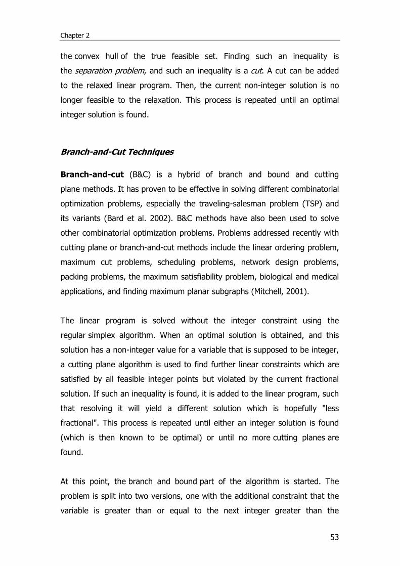
Chapter 2
53
the convex hull of the true feasible set. Finding such an inequality is
the separation problem, and such an inequality is a cut. A cut can be added
to the relaxed linear program. Then, the current non-integer solution is no
longer feasible to the relaxation. This process is repeated until an optimal
integer solution is found.
Branch-and-Cut Techniques
Branch-and-cut (B&C) is a hybrid of branch and bound and cutting
plane methods. It has proven to be effective in solving different combinatorial
optimization problems, especially the traveling-salesman problem (TSP) and
its variants (Bard et al. 2002). B&C methods have also been used to solve
other combinatorial optimization problems. Problems addressed recently with
cutting plane or branch-and-cut methods include the linear ordering problem,
maximum cut problems, scheduling problems, network design problems,
packing problems, the maximum satisfiability problem, biological and medical
applications, and finding maximum planar subgraphs (Mitchell, 2001).
The linear program is solved without the integer constraint using the
regular simplex algorithm. When an optimal solution is obtained, and this
solution has a non-integer value for a variable that is supposed to be integer,
a cutting plane algorithm is used to find further linear constraints which are
satisfied by all feasible integer points but violated by the current fractional
solution. If such an inequality is found, it is added to the linear program, such
that resolving it will yield a different solution which is hopefully "less
fractional". This process is repeated until either an integer solution is found
(which is then known to be optimal) or until no more cutting planes are
found.
At this point, the branch and bound part of the algorithm is started. The
problem is split into two versions, one with the additional constraint that the
variable is greater than or equal to the next integer greater than the
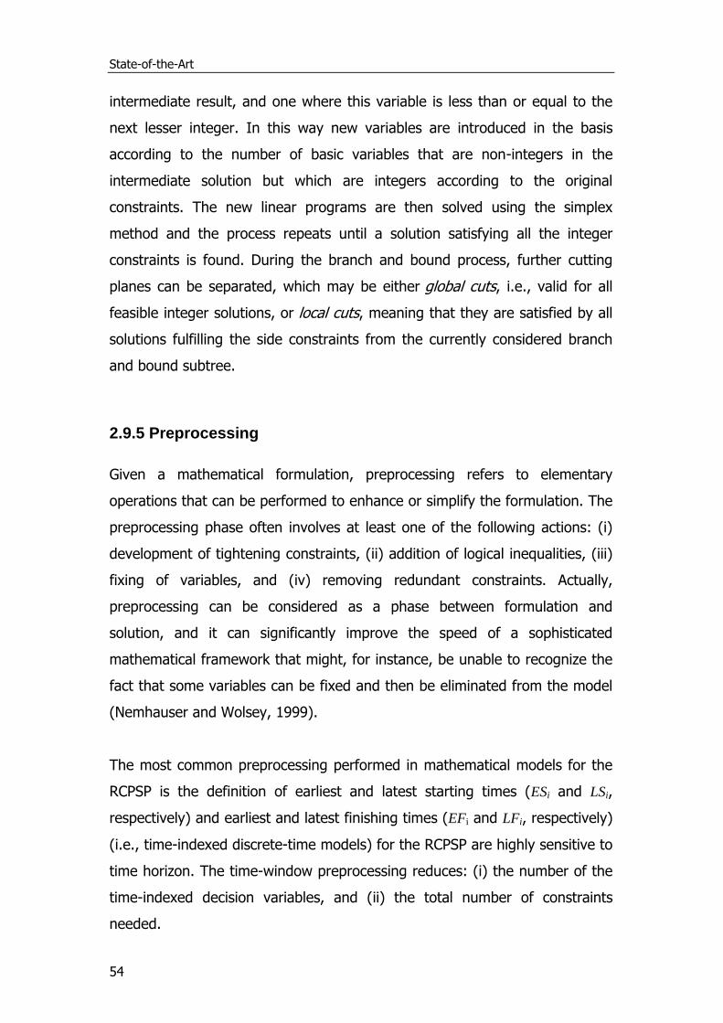
State-of-the-Art
54
intermediate result, and one where this variable is less than or equal to the
next lesser integer. In this way new variables are introduced in the basis
according to the number of basic variables that are non-integers in the
intermediate solution but which are integers according to the original
constraints. The new linear programs are then solved using the simplex
method and the process repeats until a solution satisfying all the integer
constraints is found. During the branch and bound process, further cutting
planes can be separated, which may be either global cuts, i.e., valid for all
feasible integer solutions, or local cuts, meaning that they are satisfied by all
solutions fulfilling the side constraints from the currently considered branch
and bound subtree.
2.9.5 Preprocessing
Given a mathematical formulation, preprocessing refers to elementary
operations that can be performed to enhance or simplify the formulation. The
preprocessing phase often involves at least one of the following actions: (i)
development of tightening constraints, (ii) addition of logical inequalities, (iii)
fixing of variables, and (iv) removing redundant constraints. Actually,
preprocessing can be considered as a phase between formulation and
solution, and it can significantly improve the speed of a sophisticated
mathematical framework that might, for instance, be unable to recognize the
fact that some variables can be fixed and then be eliminated from the model
(Nemhauser and Wolsey, 1999).
The most common preprocessing performed in mathematical models for the
RCPSP is the definition of earliest and latest starting times (ESi and LSi,
respectively) and earliest and latest finishing times (EFi and LFi, respectively)
(i.e., time-indexed discrete-time models) for the RCPSP are highly sensitive to
time horizon. The time-window preprocessing reduces: (i) the number of the
time-indexed decision variables, and (ii) the total number of constraints
needed.
Chapter 2
55
2.10 Time representation
In all mathematical formulations, the representation of time is an important
issue. Two main approaches are used: discrete-time and continuous-time,
depending on whether the events of the schedule can only take place at
some predefined time points , or can occur at any moment during the time
horizon of interest, respectively.
Discrete-time models are based on: (i) dividing the scheduling horizon into a
finite number of time intervals with predefined duration and, (ii) allowing the
events such as the beginning or ending of tasks to happen only at the
boundaries of these time periods (see Fig. 2.8a). Therefore, scheduling
constraints have only to be monitored at specific and known time points,
which reduces the problem complexity and makes the model structure
simpler and easier to solve, particularly when resource limitations are taken
into account. On the other hand, this type of problem simplification has two
major disadvantages. First, the size of the mathematical model as well as its
computational efficiency strongly depend on the number of time intervals
postulated, which is defined as a function of the problem data and the
desired accuracy of the solution. Note that a dense discretisation of the time
horizon would increase the number of decision variables and lead to large
combinatorial problems, which are hard to solve (or even intractable).
Second, sub-optimal or even infeasible schedules may be generated because
of the reduction of the domain of timing decisions. This time representation is
an approximation of time, with the length of each interval usually set to be
equal to the greatest common factor of activity processing times. Despite
being a simplified version of the original scheduling problem, discrete
formulations have proven to be very efficient, adaptable and convenient for a
wide variety of industrial applications, especially in those cases where a
reasonable number of intervals is sufficient to obtain the desired problem
representation.
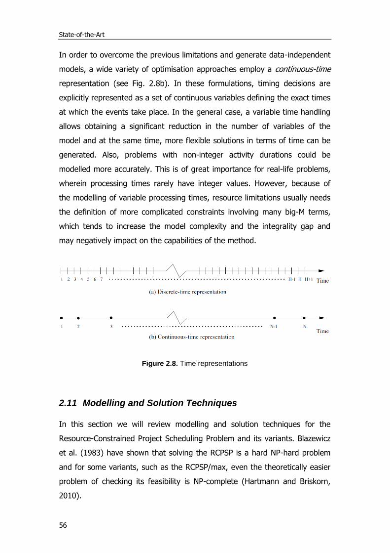
State-of-the-Art
56
In order to overcome the previous limitations and generate data-independent
models, a wide variety of optimisation approaches employ a continuous-time
representation (see Fig. 2.8b). In these formulations, timing decisions are
explicitly represented as a set of continuous variables defining the exact times
at which the events take place. In the general case, a variable time handling
allows obtaining a significant reduction in the number of variables of the
model and at the same time, more flexible solutions in terms of time can be
generated. Also, problems with non-integer activity durations could be
modelled more accurately. This is of great importance for real-life problems,
wherein processing times rarely have integer values. However, because of
the modelling of variable processing times, resource limitations usually needs
the definition of more complicated constraints involving many big-M terms,
which tends to increase the model complexity and the integrality gap and
may negatively impact on the capabilities of the method.
Figure 2.8. Time representations
2.11 Modelling and Solution Techniques
In this section we will review modelling and solution techniques for the
Resource-Constrained Project Scheduling Problem and its variants. Blazewicz
et al. (1983) have shown that solving the RCPSP is a hard NP-hard problem
and for some variants, such as the RCPSP/max, even the theoretically easier
problem of checking its feasibility is NP-complete (Hartmann and Briskorn,
2010).
Chapter 2
57
A number of solution methods, both exact and approximate have been
proposed in the literature so far. Exact techniques found in the literature rely
usually on mathematical programming formulations and specialised branch-
and-bound algorithms. Due to the high degree of complexity of RCPSPs, a
number of approximate methods such as heuristics and metaheuristics have
also been proposed in the literature.
Roughly speaking, a heuristic is a technique designed to solve a problem, or
find an approximate solution with few computational requirements, when
classic methods fail to find any exact solution. By trading optimality,
completeness, accuracy, and/or precision for speed, a heuristic can quickly
produce a solution that is good enough for solving the problem at hand. The
heuristic procedures broadly fall into two categories, namely constructive
heuristics and improvement heuristics (Demeulemeester and Herroelen,
2002). Constructive heuristics start from an empty schedule and add activities
one by one until one feasible schedule is obtained. To that purpose, the
activities are typically ranked by using priority rules which determine the
order in which the activities are added to the schedule. Improvement
heuristics, on the other hand, start from a feasible schedule that was
obtained by some constructive heuristic. Operations are performed on a
schedule which transform a solution into an improved one. These operations
are repeated until a locally optimal solution is obtained. Steepest descent,
fastest descent and iterated descent are various way of arriving in locally
optimal solutions. Some improvement heuristics try to avoid getting stuck in a
locally optimal solution by allowing an intermediate deterioration of the
project makespan. In those cases, one has to avoid the phenomenon of
cycling, i.e. repeatedly considering the same sequence of schedules. To that
purpose, several metaheuristics like tabu search, simulated annealing and
genetic algorithms have been proposed. A metaheuristic optimises a problem
by iteratively trying to improve a candidate solution with regard to a given
measure of quality. Metaheuristics make few or no assumptions about the
problem being optimized and can search very large spaces of candidate
State-of-the-Art
58
solutions. However, similar to heuristics, there is no guarantee on the quality
of the solution obtained, and it is often impossible to tell how far the current
solution is from optimality.
Finally, hybrid methods combine more than solution technique, e.g. exact and
heuristic, heuristic and metaheuristic, e.t.c.
We focus our review to solution procedures that aim at minimising the project
makespan, which (as pointed out in section 2.6.1) is the most popular and
important objective. For a thorough state-of-the-art the interested reader is
referred to the excellent works of Kolisch (1996a), Hartmann and Kolisch
(2000), Demeulemeester and Herroelen (2002), Kolisch and Hartmann
(2006), Hartmann and Briskorn (2010) and Węglarz et al. (2011).
2.11.1 RCPSP
The classical RCPSP belongs to the class of problems that are strongly NP-
hard, as demonstrated by Blazewicz et al. (1983), and since the late 1950s
most of the work in project scheduling has focused on developing solution
techniques for it. Due to its generality the classical RCPSP, has attracted most
of the project scheduling research effort. Our review, will focus on the most
important solution methods proposed in the literature.
Exact methods
Starting with exact methods for the RCPSP, a very early discrete-time
mathematical model for the RCPSP was presented by Pritsker et al. (1969).
This Binary Integer Programming (BIP) formulation was designed for multi-
project scheduling, but can also be used for the single-project case. It is
based on the definition of binary variables, which specify if an activity starts
processing at a specific time point or not. Activities have a resource demand
at the time point that they start processing, and no resource demand at the
Chapter 2
59
time point of their completion. The MILP model accommodated a wide range
of conditions and supported objectives for minimizing the makespan and
minimizing the total lateness. No computational results are available for this
early study.
Christofides et al. (1987) developed a formulation similar to Pritsker et al.,
which mainly differs in how they formulate the precedence constraints with
the new precedence constraints being disaggregated expressions of
Pritsker’s. They introduced CAT, a depth-first branch-and-bound procedure
that generates a branch-and-bound tree, whose nodes correspond to semi-
active feasible partial schedules. The procedure only branches to resolve a
resource conflict. The reported computational results are on randomly
generated problems involving up to 25 activities and 3 resources.
Kaplan (1988) developed a different time-indexed discrete-time BIP
formulation for the preemptive version of the RCPSP, which can easily be
adopted to the standard RCPSP. It is based on defining a single type of binary
variables that specify if activities are in process in each time period, thus
allowing a much simpler definition of the resource constraints. In this
formulation, the dummy start and end activities are assigned durations equal
to 1 which have to be considered when performing the forward and the
backward pass, respectively. Moreover, transitive precedence relationships
are introduced between activities.
The very efficient algorithm, presented by Demeulemeester and Herroelen
(1992, 1997a) is an extension of the depth-first branch and bound approach
of Christofides et al. (1987). The new nodes in the enumeration tree are
created by considering sets of activities which are delayed. Two dominance
rules are used to prune the enumeration tree. The first one is a variation of
the left-shift dominance rule. The second one makes use of a “cutest”, i.e.
unscheduled activities for which all predecessors belong to the partial
schedule. Bounding is performed with the precedence-based and the critical-
State-of-the-Art
60
sequence-based lower bound used by Stinson et al. (1978), and the
weighted-node-packing-bound of Mingozzi et al. (1998).
Two formulations with an exponential number of variables are those of
Alvarez-Valdés and Tamarit (1993) and Mingozzi et al. (1998), making them
more useful when calculating lower bounds. The first one proposes a
continuous-time formulation based on the definition of a set IS of all minimal
resource incompatible sets S. A resource incompatible set is a set of activities
between which no precedence relation exists, but which would violate the
resource constraints, if performed in parallel. Their model is based on the
definition of sequencing binary variables which define the sequencing of
activities. The second one by Mingozzi et al. (1998), is a discrete-time BIP
formulation based on feasible subsets, that is activities that can be
simultaneously executed without violating resource or precedence
constraints.
Klein (2000) proposed a discrete-time BIP model with precedence and
resource constraints similar to those presented by Kaplan (1988). A single
type of binary variables is used, specifying if an activity starts at the
beginning of time point t or earlier.
Artigues et al. (2003) proposed a continuous MIP formulation based on
sequencing and resource flow variables. Starting time continuous variables
are defined for each activity. In addition, sequencing binary variables are
introduced to define the sequence between any pair of activities. Finally,
resource flow continuous variables are defined to denote the quantity of
resource directly transferred from one activity (at its completion) to another
(at the beginning of its processing). Notice that in this mathematical
formulation the resource requirements of the dummy activities are equal to
the maximum available capacity, instead of setting them to zero. That way,
the start dummy activity acts as a resource source while the end dummy
activity plays the role of a resource sink.
Chapter 2
61
Schmidt and Grossmann (1996) proposed a single mode, slot-based
continuous-time formulation with no resource constraints for the optimal
scheduling of testing tasks in the new product development process of an
agricultural chemical or pharmaceutical company. In subsequent work, the
focus changed to the development of realistic models that could be solved for
large-scale problems. Jain and Grossmann (1999) extended Schmidt’s work
by including resource constraints, and Maravelias and Grossmann (2004)
further extended that model by allowing the allocation of different levels of
resources and capacity expansion. On the same problem of scheduling of
clinical trials in the pharmaceutical research and development pipeline, Colvin
and Maravelias (2008) developed a basic resource-constrained multi-stage
stochastic programming formulation (MSSP) model which was extended in
Colvin and Maravelias (2009) to account for outlicensing and resource
planning including outsourcing. In their recent work, Colvin and Maravelias
(2010) focused on the development of new results that lead to smaller MSSP
mixed-integer programming (MIP) formulations and the development of a
solution algorithm to address problems that cannot be generated using
commercial tools. Papageorgiou, Rotstein, and Shah (2001) proposed a MILP
model assuming that enough resources are always available. The formulation
integrates the selection of both a product development and introduction
strategy and a capacity planning and investment strategy. Levis and
Papageorgiou (2004) proposed a mathematical model, which is an extension
of the previous work, determining both the product portfolio and the multi-
site capacity planning in the face of uncertain clinical trials outcomes while
taking into account the trading structure of the company.
Recently, Koné et al. (2011) introduced two different event-based
continuous-time MIP formulations wherein the decision variables are indexed
using event points instead of time points, that correspond to start or end
times of activities. The Start/End Event-based (SEE) formulation, which is a
variant of the event-based formulation proposed in Zapata et al. (2008), and
the On/Off Event-based (OOE) formulation. The variables in such
State-of-the-Art
62
formulations are fewer than in time-indexed ones, since they are not a
function of the time horizon. They compared the event-based formulations
with three other formulations issued from the literature, two of which
(Pritsker et. al., 1969 and Christofides et al., 1987) use time-indexed
variables, and a third formulation (Artigues et al., 2003) that uses sequential
variables. The computational results proved that the formulation proposed by
Christofides et al. (1987) yields better results for exact solving on traditional
test instances. The event-based formulations (more particularly the OOE) and
the one by Artigues et al. (2003), have the advantage of solving more easily
the instances involving very large scheduling horizons. Finally, their OOE
formulation consistently outperformed the SEE on all tested instance sets.
Approximate methods
A number of different approximate procedures have been developed for the
RCPSP. Priority-rule-based scheduling is made up of two components: A
schedule generation scheme (SGS) and a priority rule. Two different schemes
for the generation of feasible schedules can be distinguished (see Kolisch,
1996a): the serial and the parallel method, respectively. Both generate a
feasible schedule by extending a partial schedule in a stage-wise fashion. In
each stage the generation scheme forms the set of all schedulable activities,
called the decision set. A specific priority rule is then employed in order to
choose one activity from the decision set which will be scheduled. While the
decision set of the serial method is made up of all currently unscheduled
activities whose predecessors have already been scheduled, the parallel
method defines the set by including all the precedence- and resource-feasible
unscheduled activities which can be started at the schedule time. Depending
on the number of passes performed, and hence the number of schedules
generated, single- and multi-pass approaches can be distinguished. A number
of such heuristics along with a computational study are reported by Kolisch
(1996a).
Chapter 2
63
Truncated branch-and-bound methods do not explore the entire enumeration
tree, instead only a partial exploration is performed. An example of such a
method is the work of Alvarez-Valdes and Tamarit (1989) that makes use of
the enumeration tree as presented in Christofides et al. (1987), i.e., nodes
consist of sets of activities which have to be delayed. Instead of enumerating
all offspring nodes, the heuristic implicitly or explicitly chooses one node.
Kochetov and Stolyar (2003) devised an evolutionary algorithm which
combines genetic algorithm, path relinking, and tabu search. Solutions are
evolved and diversified in a genetic way. Evolution is done by choosing two
solutions from the pool and constructing the path of solutions linking the
selected solutions (path relinking). The best solution from the path is chosen
and improved via tabu search. The latter employs a neighborhood where the
activity list is divided in three parts. For the first and the last part the serial
SGS is employed while for the mid part the parallel SGS is used. The best
solution from the tabu search is added to the population and the worst
solution is removed from the population.
Debels et al. (2006) proposed a new metaheuristic that combines elements
from scatter search, a generic population-based evolutionary search method,
and from a recently introduced heuristic method for the optimisation of
unconstrained continuous functions based on an analogy with
electromagnetism theory. The computational experiments show that the
procedure is capable of producing consistently good results for challenging
instances of the resource-constrained project scheduling problem and that
the algorithm outperforms previous state-of-the-art existing heuristics.
Debels and Vanhoucke (2008) presented a new genetic algorithm (GA) that is
able to provide near-optimal heuristic solutions. This GA procedure is also
extended by a so-called decomposition-based genetic algorithm (DBGA) that
iteratively solves subparts of the project. They present computational
experiments on two data sets. The first benchmark set is used to illustrate
State-of-the-Art
64
the performance of both the GA and the DBGA. The second set is used to
compare the results with current state-of-the-art heuristics and to show that
the procedure is capable of producing consistently good results for
challenging problem instances. The GA outperforms all state-of-the-art
heuristics and the DBGA further improves the performance of the GA.
Paraskevopoulos et al. (2012) proposed a new solution representation and an
evolutionary algorithm for solving the RCPSP. The representation scheme is
based on an ordered list of events, that are sets of activities that start (or
finish) at the same time. The proposed solution methodology, namely SAILS,
operates on the event list and relies on a scatter search framework. The
latter incorporates an Adaptive Iterated Local Search (AILS), as an
improvement method, and integrates an event-list based solution
combination method. AILS utilizes new enriched neighborhoods, guides the
search via a long term memory and applies an efficient perturbation strategy.
Computational results on benchmark instances of the literature indicate that
both AILS and SAILS produce consistently high quality solutions, while the
best results are derived for most problem data sets.
2.11.2 Multi-mode Resource Constrained Project Scheduling
Problem (MRCPSP)
When the solution has to additionally determine the assignment of modes
(MRCPSP), further complexity is added since the solution search space is
enlarged. The MRCPSP is NP-hard in the strong sense being a generalization
of the RCPSP. Moreover, for more than one non-renewable resources the
problem of finding a feasible solution is already NP-complete (Kolisch, 1995).
Exact methods
Exact methods for the MRCPSP include the formulation of Talbot (1982),
which considers the objective of minimizing the makespan under a given
Chapter 2
65
budget, and minimizing the total non-renewable resource consumption under
the presence of a project due date.
Sprecher et al. (1997) extended the enumeration scheme of Demeulemeester
and Herroelen (1992) for the single-mode to the multi-mode RCPSP.
Hartmann and Drexl (1998) generalised the exact procedure of Stinson et al.
(1978) to the multi-mode context.
Zhu et al. (2006) proposed a branch-and-cut method based on Christofides et
al. formulation (1987) for the MRCPSP. The primary contribution of their
research aimed at the development of several techniques for accelerating the
solution process, including variable reduction, cut generation, and bound
tightening. In addition, a high-level search strategy referred to as local
branching was applied to find good feasible solutions in the early stages of
the computations. Their work gave very competitive results on benchmark
problems and remains the best-performing exact method to date.
Sabzehparvar et al. (2008) presented a continuous-time formulation for the
MRCPSP with Generalized Precedence Relations (MRCPSP-GPR) with mode-
dependent minimal or maximal time lags. The proposed model has been
inspired by the rectangle packing problems, but it has no need for a feasible
solution to start. Their computational study consisted of a set of 60 test
problems.
In a recent paper from the process systems industry, Zapata et al. (2008)
developed 3 different MILP models to address large-scale Multi-mode
Resource Constrained Multi-Project Scheduling Problems (multi-mode
RCMPSP), using continuous divisible resources and continuous time. The
“curse” of dimensionality of the problem (indexing of task execution modes,
indexing of time periods, and the discrete character of the resources), limits
the exact solution of the formulations to very small systems. Each of the 3
proposed models handles the time domain in a different way, but the
State-of-the-Art
66
computational results show that hat despite the theoretical advantages of the
strategies used they are limited to problems in the same range of applicability
of conventional multi-mode formulations.
Approximate methods
Starting with approximate solution procedures, Hartmann (2001) presented
an efficient genetic algorithm, with the genetic encoding based on a
precedence feasible list of activities and a mode assignment. After defining
the related crossover, mutation, and selection operators, they use a local
search extension to improve the schedules found by the basic genetic
algorithm.
Alcaraz et al. (2003) proposed another genetic algorithm with slightly worse
performance than that of Hartmann, but with a better fitness function.
Jarboui et al. (2008) propose a combinatorial Particle Swarm Optimisation
(CPSO) algorithm that first generates an assignment of modes to activities
which is called particle and then uses a local search to optimize the
sequences when a new assignment is made.
Van Peteghem and Vanhoucke (2010) designed a genetic algorithm which
uses two populations, one with left-justified schedules and one with right-
justified schedules. They also introduced an extended serial schedule
generation scheme, which improves the mode selection by choosing that
feasible mode of a certain activity that minimises the finish time of that
activity. According to their computational results, their algorithm outperforms
all prior algorithms in literature, within reasonable computation times.
Coelho and Vanhoucke (2011) developed a new algorithm that splits the
problem type into a mode assignment and a single mode project scheduling
step. The mode assignment step is solved by a satisfiability (SAT) problem
Chapter 2
67
solver and returns a feasible mode selection to the project scheduling step.
The project scheduling step is solved using an efficient meta-heuristic
procedure from literature to solve the RCPSP. Computational results show
that the procedure can report similar or sometimes even better solutions than
the algorithm of Van Peteghem and Vanhoucke (2010), although it often
requires a higher CPU time. This makes the considered genetic algorithm
approach the most powerful heuristic developed up to now.
2.11.3 RCPSP/max
The addition of maximal time lags to the classical RCPSP, significantly
increases the complexity of the problem. Moreover, the generation of
problem instances could be problematic because infeasible problems might be
generated. The RCPSP/max is an NP-hard problem and even the theoretically
easier problem of checking its feasibility is NP-complete (Hartmann and
Briskorn, 2010).
The RCPSP/max has been mostly studied under the objective of minimising
the project makespan. Non-regular objectives functions, such as resource
levelling and net present value problems, are also considered in various
works (Neumann and Zimmermann 1999, 2000 and Rieck et al., 2012). For
an extensive review of project scheduling problems with time windows the
interested reader is referred to Neumann, Schwindt and Zimmermann (2002,
2003).
Exact methods
Most exact solution procedures for the RCPSP/max in the literature are
usually branch-and-bound algorithms.
The early work of Bartusch et al. (1988), mainly aimed at the mathematical
properties of the problem, but also proposed a B&B procedure that extends
State-of-the-Art
68
the set of precedence relations to eliminate all reduced forbidden sets in an
initial time-feasible solution. The computational results are limited to a single
bridge construction project.
Demeulemeester and Herroelen (1997b) extend their DH-procedure to the
Generalized Resource-Constrained Project Scheduling Problem (GRCPSP),
which only deals with minimal time lags.
De Reyck and Herroelen (1998) proposed a hybrid depth-first/laser beam
search B&B algorithm. Schwindt (1998a) delayed activities by adding special
precedence constraints (i.e., disjunctive precedence constraints) between
sets of activities, unlike the previous two methods which used activity pairs.
Fest et al. (1998) proposed a similar approach, but instead of introducing
precedence constraints, the resource conflicts were resolved only locally by a
dynamic update of job release dates.
Dorndorf et al. (2000) presented a time-oriented B&B algorithm that uses
constraint-propagation techniques which actively exploit the temporal and
resource constraints of the problem in order to reduce the search space.
Recently, Bianco and Caramia (2012b) proposed a B&B algorithm that utilises
a new mathematical formulation. The mathematical uses a discrete-time
approach with one continuous and two binary variables. Continuous variable
xit represents the percentage of activity i executed till the end of time period
t. Binary variables itit fs / assume value 1 for every t , where τ is the time
activity i started/finished, and value 0 otherwise. Lower bounds are calculated
through a Langrangian relaxation of the former model. Their extensive
computational comparison with known lower bounds and exact methods,
displays the efficiency of their algorithm in the calculation of bounds and
solutions.
Chapter 2
69
Approximate methods
Some representative approximate approaches are mentioned below. Franck
and Neumann (1998) proposed a two step method: (a) a sophisticated
decomposition analysis is performed to identify critical sub-components which
can be scheduled independently, and (b) the scheduled sub-components
(partial schedules) are integrated into one using a set of priority rules.
Cesta et al. (2002) presented an algorithm based on a constraint satisfaction
problem solving search procedure. Cicirello and Smith (2004) described a
framework for integrating multiple heuristics within a stochastic sampling
search algorithm, and validated it on the RCPSP/max. Smith (2004)
developed a non-systematic hybrid that combines squeaky wheel optimisation
with an effective window-based conflict resolution mechanism.
Finally, Ballestin et al. (2011) proposed an evolutionary algorithm that utilises
the double justification technique of Valls et al. (2005) to improve solutions
generated in the evolutionary process.
2.12 Modelling and Optimisation Software
Solving mathematical programming problems without the use of a computer
is extremely hard even for small cases. Available commercial software and
hardware have evolved greatly the last few years, reducing running times,
computational costs and solving larger problems. Examples of commercial
modelling and optimisation software with common features are GAMS,
AIMMS, AMPL, Gurobi and ILOG. GAMS is the most commonly used tool in
the Process Systems Engineering community, with which we attempt to
exchange methods in this thesis. The rest of this section presents the GAMS
system and CPLEX solver that were selected to solve the optimisation
problems developed.
State-of-the-Art
70
2.12.1 General Algebraic Modelling System (GAMS)
The General Algebraic Modelling System (GAMS) is a high-level
modelling system for mathematical optimisation. It is designed for modelling
and solving linear, nonlinear, and mixed-integer optimisation problems. GAMS
was the first algebraic modelling language (AML) and is formally similar to
commonly used fourth-generation programming languages. It is available for
use on various computer platforms and the models are portable from one
platform to another.
GAMS allows the users to implement a sort of hybrid algorithms combining
different solvers in a seamless way. Models are described in concise algebraic
statements which are easy to read, both for humans and machines. Although
initially designed for applications related to economics and management
science, it has a large community of users from various backgrounds of
engineering and science.
GAMS contains an integrated development environment (IDE) which is
connected to a group of third-party optimisation solvers, such as BARON,
COIN solvers, CONOPT, CPLEX, DICOPT, GUROBI, MOSEK, SNOPT, and
XPRESS. The GAMS system is tailored for complex, large-scale modelling
applications and allows the user to build large maintainable models that can
be adapted to new situations.
According to Rosenthal (2012) and Castillo, Conejo, Pedregal, García, and
Alguaci (2001), some of the more remarkable features of GAMS algebraic
modelling language are:
The model representation is analogous to the mathematical description
of the problem. Therefore, learning GAMS programming language is
almost natural for those working in the optimisation field. Additionally,
GAMS is formally similar to commonly used programming languages.
Chapter 2
71
Models are described in compact and concise algebraic statements
which are easy for both humans and machines to read.
The modelling task is completely apart from the solving procedure.
Once the model of the system in question has been built, one can
choose among the diverse solvers available to optimise the problem.
Allows changes to be made in model specifications simply and safely.
Allows unambiguous statements of algebraic relationships.
Permits model descriptions that are independent of solution
algorithms.
All data transformations are specified concisely and algebraically. This
means that all data can be entered in their most elemental form and
that all transformations made in constructing the model and in
reporting are available for inspection.
The ability to model small size problems and afterwards transform
them into large-scale problems without significantly varying the code.
Decomposition algorithms can be programmed in GAMS by using
specific commands, thus not requiring additional software.
GAMS imports/exports data from/to Microsoft EXCEL. Additionally,
GAMS can be easily linked with MATLAB (The Mathworks, 1998) using
the matgams library (Ferris, 1999) if some special data manipulation is
needed.
2.12.2 CPLEX Solver
IBM ILOG CPLEX, which is often informally referred to simply as CPLEX, is an
optimisation solver package. The CPLEX Optimiser was named after the C
programming language in which it was implemented and the Simplex
method. However, today it provides additional methods for mathematical
programming and offers interfaces other languages such as C++, C#, and
Java, Python (through the C interface). Additional connectors to Microsoft
Excel and MATLAB are also provided. The CPLEX Optimiser is accessible
through independent modelling systems such as AIMMS, AMPL, GAMS, MPL,
State-of-the-Art
72
OpenOpt, OptimJ and TOMLAB. Specifically for GAMS, GAMS/CPLEX is a
solver that allows users to combine the high level modelling capabilities of
GAMS with the power of CPLEX optimisers.
The CPLEX Optimiser is designed to solve large, difficult problems quickly and
with minimal user intervention. Access is provided (subject to proper
licensing) to solution algorithms for linear, integer, quadratically constrained
and mixed integer programming problems.
While numerous solving options are available, GAMS/CPLEX automatically
calculates and sets most options at the best values for specific problems. It is
worth mentioning that for problems with integer variables CPLEX uses a
branch-and-cut algorithm which solves a series of LP subproblems. Because a
single mixed integer problem generates many subproblems, even small MIP
problems can be very computationally intensive and require significant
amounts of physical memory.
2.13 Concluding Remarks
In this chapter, various aspects of the RCPSP and its variants have been
reviewed, along with test instances commonly used by researchers for
benchmarking. Also, major optimisation techniques and tools used
throughout this thesis have been presented. The main concepts beneath each
method have been briefly described in order to provide the reader with a
general understanding of the theory involved into the solution approaches.
Finally, exact and approximate solution procedures for the RCPSP, from the
literature have been thoroughly reviewed.
At this point, it is worth noticing that the process of building a mathematical
model is often considered to be as important as solving it because this
process provides insight about how the system works and helps organise
essential information about it. Models of the real world are not always easy to

Chapter 2
73
formulate because of the richness, variety, and ambiguity that exists in the
real world or because of our ambiguous understanding of it. As a result,
building up concise, useful and efficient mathematical models/approaches is a
very difficult and challenging task and this thesis has placed particular
attention towards this direction.

74
Chapter 3
75
Chapter 3
RTN-based MILP Formulations for Single- and
Multi-Mode Resource-Constrained Project
Scheduling Problems
This chapter presents new mixed-integer linear programming models for the
deterministic single- and multi-mode resource-constrained project scheduling
problem with renewable and non-renewable resources. The modelling
approach relies on the Resource-Task Network (RTN) representation, a
network representation technique used in process scheduling problems,
based on continuous time models. First, we propose new RTN-based network
representation methods, and then we efficiently transform them into
mathematical formulations including a set of constraints describing
precedence relations, different types of resources and multiple objectives.
Finally, the applicability of the proposed formulations is illustrated using
several example problems under the most commonly addressed objective, the
makespan minimization.
3.1 Introduction
The main scope of this chapter is to extend and therefore apply modelling
and network representation techniques used in the process industry to RCPSP
and MRCPSP problems.
A general project consists of a set of interconnected activities and resources,
logically linked. These activities usually have to be performed for a successful
project completion. However, there may exist alternatives for some activities,
which vary in aspects such as duration, cost and required sets of resources.
Since resources impose restrictions to project scheduling, they must be
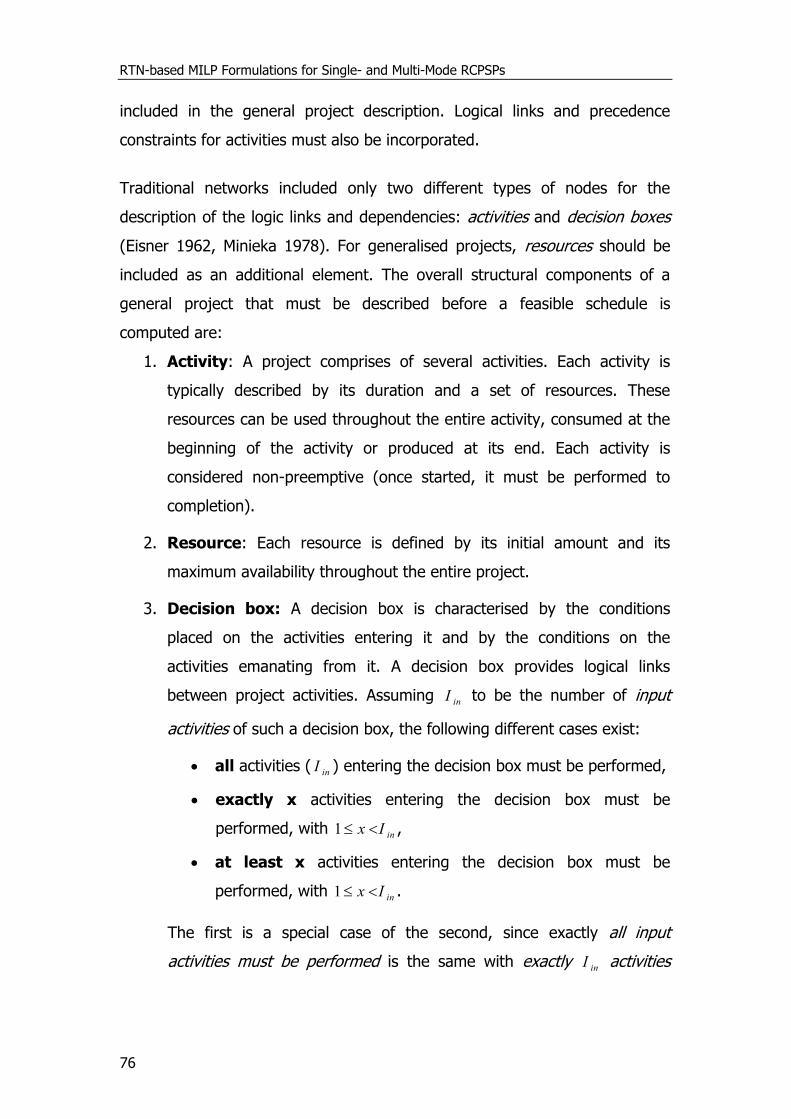
RTN-based MILP Formulations for Single- and Multi-Mode RCPSPs
76
included in the general project description. Logical links and precedence
constraints for activities must also be incorporated.
Traditional networks included only two different types of nodes for the
description of the logic links and dependencies: activities and decision boxes
(Eisner 1962, Minieka 1978). For generalised projects, resources should be
included as an additional element. The overall structural components of a
general project that must be described before a feasible schedule is
computed are:
1. Activity: A project comprises of several activities. Each activity is
typically described by its duration and a set of resources. These
resources can be used throughout the entire activity, consumed at the
beginning of the activity or produced at its end. Each activity is
considered non-preemptive (once started, it must be performed to
completion).
2. Resource: Each resource is defined by its initial amount and its
maximum availability throughout the entire project.
3. Decision box: A decision box is characterised by the conditions
placed on the activities entering it and by the conditions on the
activities emanating from it. A decision box provides logical links
between project activities. Assuming inI to be the number of input
activities of such a decision box, the following different cases exist:
all activities ( inI ) entering the decision box must be performed,
exactly x activities entering the decision box must be
performed, with inIx 1 ,
at least x activities entering the decision box must be
performed, with inIx 1 .
The first is a special case of the second, since exactly all input
activities must be performed is the same with exactly inI activities
Chapter 3
77
must be performed. This enables us to group the all input condition
with the exactly x, by allowing x to take the value inI .
The input condition must be satisfied for some of the activities
emanating from the decision box to be performed. A decision box may
have two different output logics:
at least one activity emanating from the decision box can be
performed,
exactly one activity emanating from the decision box can be
performed.
4. Project end: The simplest way of describing the project end is as a
special decision box with one or more activities entering it.
The chapter is organised as follows. In section 3.2, a new network
representation of project scheduling problems based on the RTN concept is
presented. In sections 3.3 and 3.4 we propose new MILP formulations for
RCPSPs and MRCPSPs, including precedence relations, different types of
resources, time, and other constraints. Afterwards, the applicability of the
proposed formulations on several project scheduling problems is
demonstrated in section 3.5. Finally, concluding remarks are drawn in section
3.6.
3.2 A new network representation for the RCPSP
The RTN process representation although simple, can describe a very wide
variety of process scheduling problems (Pantelides, 1994). Indeed, it has
been extensively used in the process scheduling literature (e.g. Castro et al.
2001, 2004). Its bipartite directed graph for general processes consists of
resources, represented as circles and tasks/activities, represented as
rectangles. A task/activity consumes and/or produces a set of resources that
can be anything from raw materials, intermediate and final products to
manpower and processing equipment. A new network representation method
RTN-based MILP Formulations for Single- and Multi-Mode RCPSPs
78
is proposed, based on the RTN, that can express more complex activity
precedence relations, than the AoN and AoA representations.
3.2.1 Conversion of General Projects to RTN form
Creating a mathematical formulation based on the RTN, requires the
definition of a framework that converts the general project characteristics
aforementioned to their equivalent RTN components. Some conventions are
easier than others, for example Activities correspond to Tasks and Project
Resources to RTN Resources. On the other hand, Decision Boxes are more
complex and they will be modelled as Resources, with specific values on their
following parameters:
1. the activity consumption and production coefficients ( ri and ri ) and
2. the minimum and maximum excess levels ( min
rR and max
rR )
Special consideration will be given to Project End translation. The Project End
is treated as a special Decision Box, which in turn is converted to an RTN
Resource.
Precedence Constraints
Projects consist of coordinated and controlled activities with start and finish
times. To achieve the required execution sequence, precedence constraints
on each activity are imposed. These constraints will be modelled indirectly, in
the proposed representation, by adding a new type of resource, called Logical
and adjusting the quantities consumed and produced by each activity.
So, besides the physical resource requirements, each activity requires one
unit of the logical resource assigned to it. This unit is produced by the
activity’s immediate predecessor(s) in equal quantities and is addressed by
properly adjusting the production coefficients ( ri ) for the preceding activities
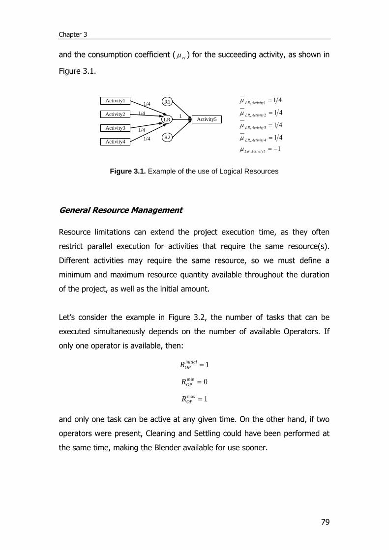
Chapter 3
79
and the consumption coefficient ( ri ) for the succeeding activity, as shown in
Figure 3.1.
Figure 3.1. Example of the use of Logical Resources
General Resource Management
Resource limitations can extend the project execution time, as they often
restrict parallel execution for activities that require the same resource(s).
Different activities may require the same resource, so we must define a
minimum and maximum resource quantity available throughout the duration
of the project, as well as the initial amount.
Let’s consider the example in Figure 3.2, the number of tasks that can be
executed simultaneously depends on the number of available Operators. If
only one operator is available, then:
1initial
OPR
0min OPR
1max OPR
and only one task can be active at any given time. On the other hand, if two
operators were present, Cleaning and Settling could have been performed at
the same time, making the Blender available for use sooner.
Activity3
LR
Activity1
Activity4
Activity2
1/4
1/4
1/4
1/4
Activity5
1
R2
R1
1
41
41
41
41
5,
4,
3,
2,
1,
ActivityLR
ActivityLR
ActivityLR
ActivityLR
ActivityLR
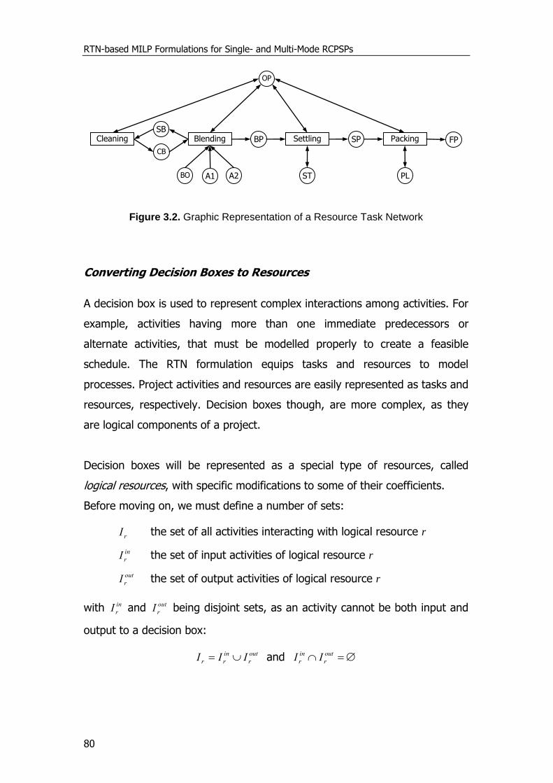
RTN-based MILP Formulations for Single- and Multi-Mode RCPSPs
80
Figure 3.2. Graphic Representation of a Resource Task Network
Converting Decision Boxes to Resources
A decision box is used to represent complex interactions among activities. For
example, activities having more than one immediate predecessors or
alternate activities, that must be modelled properly to create a feasible
schedule. The RTN formulation equips tasks and resources to model
processes. Project activities and resources are easily represented as tasks and
resources, respectively. Decision boxes though, are more complex, as they
are logical components of a project.
Decision boxes will be represented as a special type of resources, called
logical resources, with specific modifications to some of their coefficients.
Before moving on, we must define a number of sets:
rI the set of all activities interacting with logical resource r
in
rI the set of input activities of logical resource r
out
rI the set of output activities of logical resource r
with in
rI and out
rI being disjoint sets, as an activity cannot be both input and
output to a decision box:
out
r
in
rr III and out
r
in
r II
Cleaning Blending
Settling Packing
OP
BO A2
SB
CB
BP SP
ST PL
FP
A1
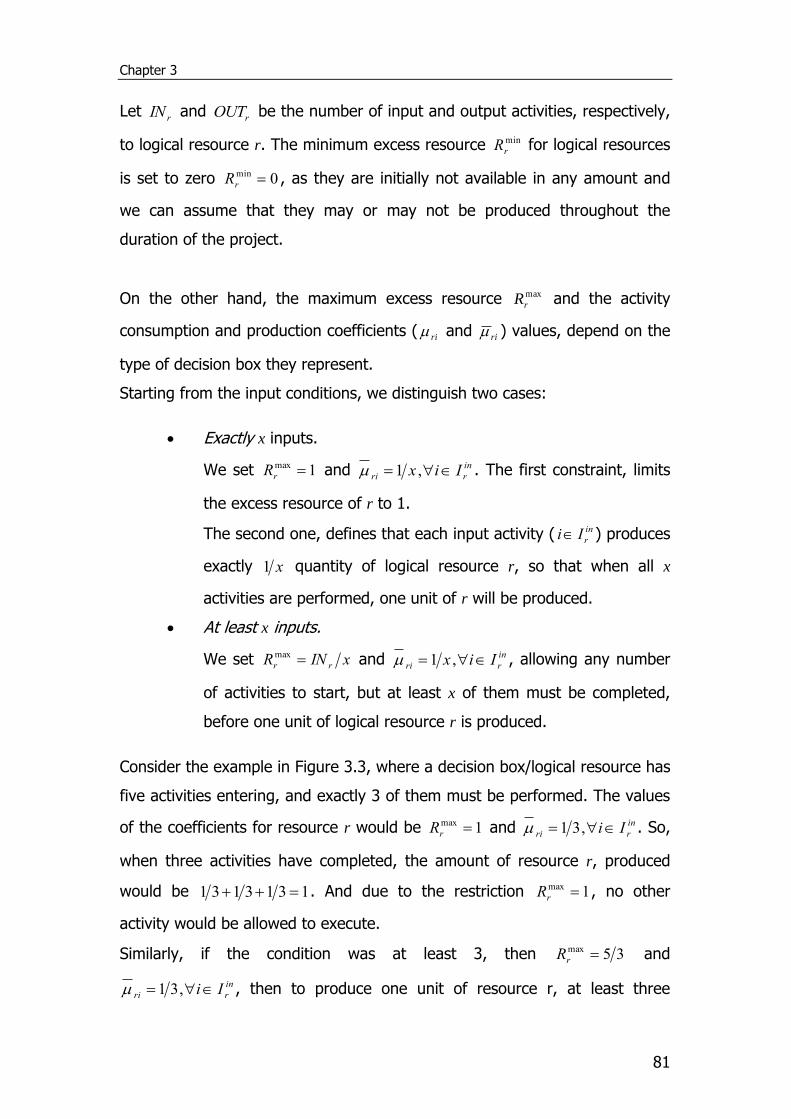
Chapter 3
81
Let rIN and rOUT be the number of input and output activities, respectively,
to logical resource r. The minimum excess resource min
rR for logical resources
is set to zero 0min rR , as they are initially not available in any amount and
we can assume that they may or may not be produced throughout the
duration of the project.
On the other hand, the maximum excess resource max
rR and the activity
consumption and production coefficients ( ri and ri ) values, depend on the
type of decision box they represent.
Starting from the input conditions, we distinguish two cases:
Exactly x inputs.
We set 1max rR and in
rri Iix ,1 . The first constraint, limits
the excess resource of r to 1.
The second one, defines that each input activity ( in
rIi ) produces
exactly x1 quantity of logical resource r, so that when all x
activities are performed, one unit of r will be produced.
At least x inputs.
We set xINR rr max and in
rri Iix ,1 , allowing any number
of activities to start, but at least x of them must be completed,
before one unit of logical resource r is produced.
Consider the example in Figure 3.3, where a decision box/logical resource has
five activities entering, and exactly 3 of them must be performed. The values
of the coefficients for resource r would be 1max rR and in
rri Ii ,31 . So,
when three activities have completed, the amount of resource r, produced
would be 1313131 . And due to the restriction 1max rR , no other
activity would be allowed to execute.
Similarly, if the condition was at least 3, then 35max rR and
in
rri Ii ,31 , then to produce one unit of resource r, at least three
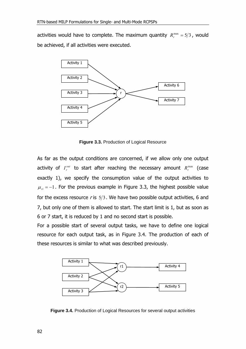
RTN-based MILP Formulations for Single- and Multi-Mode RCPSPs
82
activities would have to complete. The maximum quantity 35max rR , would
be achieved, if all activities were executed.
Figure 3.3. Production of Logical Resource
As far as the output conditions are concerned, if we allow only one output
activity of out
rI to start after reaching the necessary amount max
rR (case
exactly 1), we specify the consumption value of the output activities to
1ri . For the previous example in Figure 3.3, the highest possible value
for the excess resource r is 35 . We have two possible output activities, 6 and
7, but only one of them is allowed to start. The start limit is 1, but as soon as
6 or 7 start, it is reduced by 1 and no second start is possible.
For a possible start of several output tasks, we have to define one logical
resource for each output task, as in Figure 3.4. The production of each of
these resources is similar to what was described previously.
Figure 3.4. Production of Logical Resources for several output activities
Activity 3
r1
Activity 1
Activity 2
Activity 5
Activity 4
r2
Activity 3
r
Activity 5
Activity 1
Activity 4
Activity 2
Activity 7
Activity 6

Chapter 3
83
After the input conditions are satisfied, resources r1 and r2 are available in
their necessary amounts and the output tasks can be performed.
The possible combinations for input and output conditions are:
Exactly x – exactly one
At least x – exactly one
Exactly one – at least one
Exactly x – at least one
At least x – at least one
These possible combinations can be described by the two networks of Figures
3.5 and 3.6.
Figure 3.5. Conditions Exactly x/At least x - Exactly one and Exactly one - At least
one
A decision box with output condition Exactly 1, is represented using one only
one new logical resource. This case corresponds to Figure 3.5. A decision box
with input condition Exactly 1, can also be represented as depicted in Figure
3.5, but we have to distinguish among different output conditions. If the
output condition is also Exactly 1, we set the consumption value to 1ri ,
to allow only one output activity to start. If the output condition is At least 1,
we set the consumption value to rri OUT1 so that every output activity
receives part of the available amount 1.
Activity 3
Activity 1
Activity 2
Activity 5
r1
Activity 4
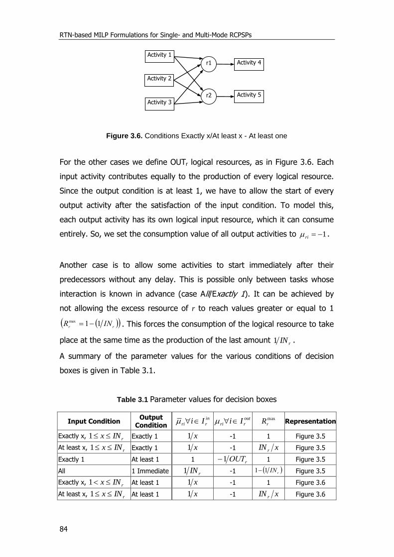
RTN-based MILP Formulations for Single- and Multi-Mode RCPSPs
84
Figure 3.6. Conditions Exactly x/At least x - At least one
For the other cases we define OUTr logical resources, as in Figure 3.6. Each
input activity contributes equally to the production of every logical resource.
Since the output condition is at least 1, we have to allow the start of every
output activity after the satisfaction of the input condition. To model this,
each output activity has its own logical input resource, which it can consume
entirely. So, we set the consumption value of all output activities to 1ri .
Another case is to allow some activities to start immediately after their
predecessors without any delay. This is possible only between tasks whose
interaction is known in advance (case All/Exactly 1). It can be achieved by
not allowing the excess resource of r to reach values greater or equal to 1
rr
INR 11max . This forces the consumption of the logical resource to take
place at the same time as the production of the last amount rIN1 .
A summary of the parameter values for the various conditions of decision
boxes is given in Table 3.1.
Table 3.1 Parameter values for decision boxes
Input Condition Output
Condition in
rri Ii out
rri Ii max
rR Representation
Exactly x, rINx 1 Exactly 1 x1 -1 1 Figure 3.5
At least x, rINx 1 Exactly 1 x1 -1 xIN r Figure 3.5
Exactly 1 At least 1 1 rOUT1 1 Figure 3.5
All 1 Immediate rIN1 -1 r
IN11 Figure 3.5
Exactly x, rINx 1 At least 1 x1 -1 1 Figure 3.6
At least x, rINx 1 At least 1 x1 -1 xIN r Figure 3.6
Activity 3
r1
Activity 1
Activity 2
Activity 5
Activity 4
r2
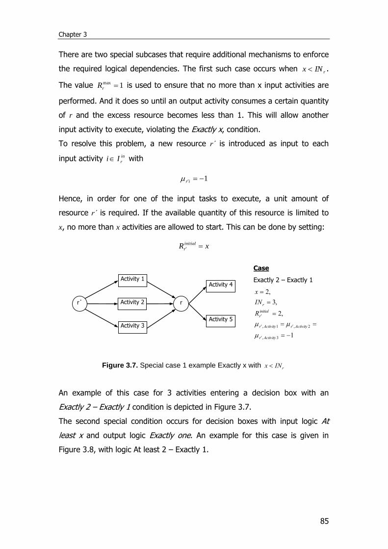
Chapter 3
85
There are two special subcases that require additional mechanisms to enforce
the required logical dependencies. The first such case occurs when rINx .
The value 1max rR is used to ensure that no more than x input activities are
performed. And it does so until an output activity consumes a certain quantity
of r and the excess resource becomes less than 1. This will allow another
input activity to execute, violating the Exactly x, condition.
To resolve this problem, a new resource r΄ is introduced as input to each
input activity in
rIi with
1ir
Hence, in order for one of the input tasks to execute, a unit amount of
resource r΄ is required. If the available quantity of this resource is limited to
x, no more than x activities are allowed to start. This can be done by setting:
xR initial
r
Figure 3.7. Special case 1 example Exactly x with rINx
An example of this case for 3 activities entering a decision box with an
Exactly 2 – Exactly 1 condition is depicted in Figure 3.7.
The second special condition occurs for decision boxes with input logic At
least x and output logic Exactly one. An example for this case is given in
Figure 3.8, with logic At least 2 – Exactly 1.
Activity 3
Activity 1
Activity 2
Activity 5
r
Activity 4
r΄
Case
Exactly 2 – Exactly 1
1
,2
,3
,2
3,
2,1,
Activityr
ActivityrActivityr
initial
r
r
R
IN
x
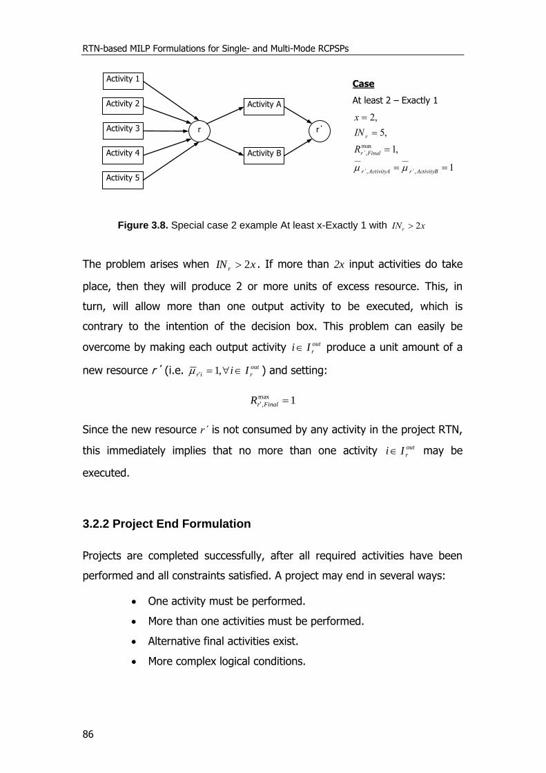
RTN-based MILP Formulations for Single- and Multi-Mode RCPSPs
86
Figure 3.8. Special case 2 example At least x-Exactly 1 with xINr 2
The problem arises when xIN r 2 . If more than 2x input activities do take
place, then they will produce 2 or more units of excess resource. This, in
turn, will allow more than one output activity to be executed, which is
contrary to the intention of the decision box. This problem can easily be
overcome by making each output activity out
rIi produce a unit amount of a
new resource r΄ (i.e. out
rir Ii ,1 ) and setting:
1max
, FinalrR
Since the new resource r΄ is not consumed by any activity in the project RTN,
this immediately implies that no more than one activity out
rIi may be
executed.
3.2.2 Project End Formulation
Projects are completed successfully, after all required activities have been
performed and all constraints satisfied. A project may end in several ways:
One activity must be performed.
More than one activities must be performed.
Alternative final activities exist.
More complex logical conditions.
Case
At least 2 – Exactly 1
1
,1
,5
,2
,,
max
,
ActivityBr΄ActivityAr΄
Finalr΄
r
R
IN
x
Activity 3
Activity 1
Activity 2
Activity 5
r
Activity 4
Activity A
Activity B
r΄
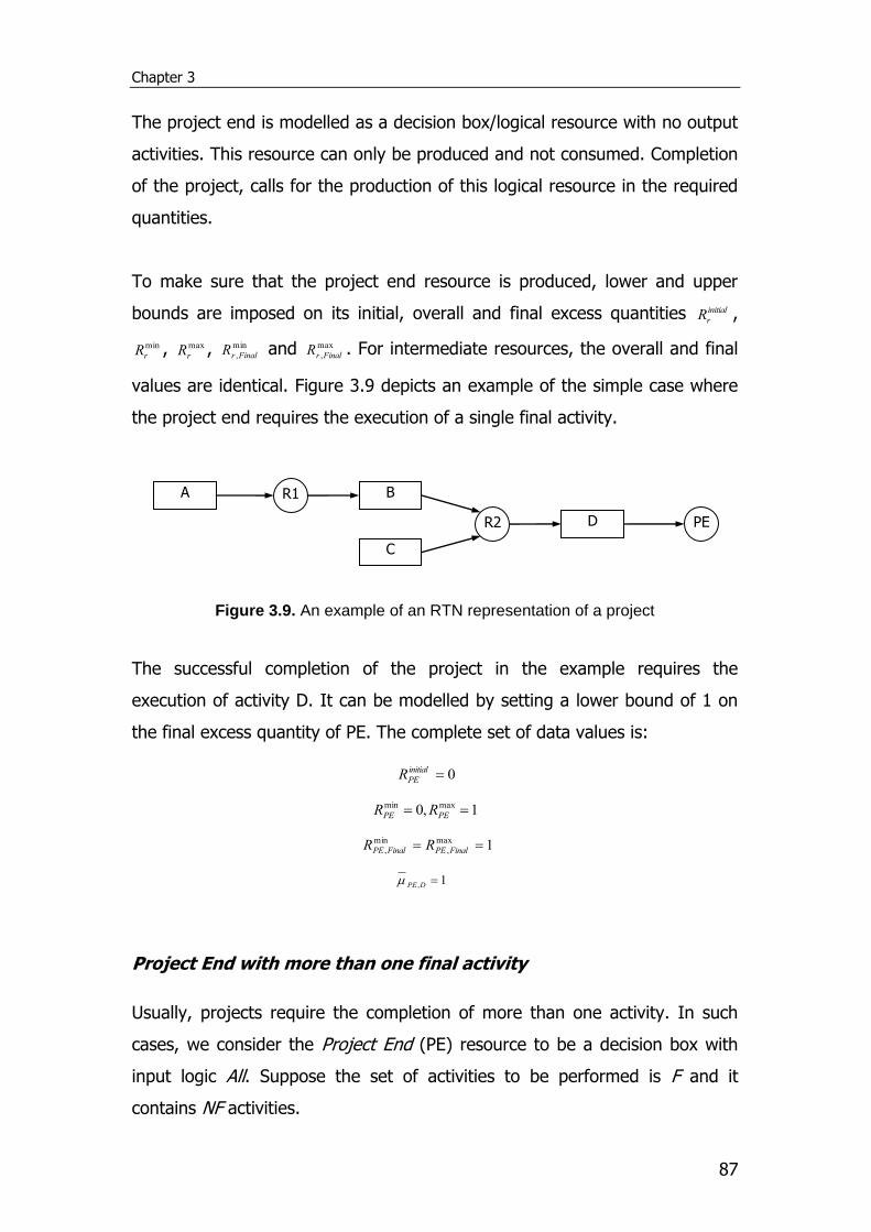
Chapter 3
87
The project end is modelled as a decision box/logical resource with no output
activities. This resource can only be produced and not consumed. Completion
of the project, calls for the production of this logical resource in the required
quantities.
To make sure that the project end resource is produced, lower and upper
bounds are imposed on its initial, overall and final excess quantities initial
rR ,
min
rR , max
rR , min
,FinalrR and max
,FinalrR . For intermediate resources, the overall and final
values are identical. Figure 3.9 depicts an example of the simple case where
the project end requires the execution of a single final activity.
Figure 3.9. An example of an RTN representation of a project
The successful completion of the project in the example requires the
execution of activity D. It can be modelled by setting a lower bound of 1 on
the final excess quantity of PE. The complete set of data values is:
0initial
PER
1,0 maxmin PEPE RR
1max
,
min
, FinalPEFinalPE RR
1, DPE
Project End with more than one final activity
Usually, projects require the completion of more than one activity. In such
cases, we consider the Project End (PE) resource to be a decision box with
input logic All. Suppose the set of activities to be performed is F and it
contains NF activities.
B
R1
R2 D
PE
A
C
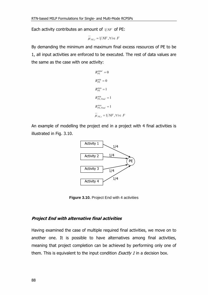
RTN-based MILP Formulations for Single- and Multi-Mode RCPSPs
88
Each activity contributes an amount of NF1 of PE:
FiNFiPE ,1,
By demanding the minimum and maximum final excess resources of PE to be
1, all input activities are enforced to be executed. The rest of data values are
the same as the case with one activity:
0initial
PER
0min PER
1max PER
1min
, FinalPER
1max
, FinalPER
FiNFiPE ,1,
An example of modelling the project end in a project with 4 final activities is
illustrated in Fig. 3.10.
Figure 3.10. Project End with 4 activities
Project End with alternative final activities
Having examined the case of multiple required final activities, we move on to
another one. It is possible to have alternatives among final activities,
meaning that project completion can be achieved by performing only one of
them. This is equivalent to the input condition Exactly 1 in a decision box.
Activity 3
PE
Activity 1
Activity 4
Activity 2
1/4
1/4
1/4
1/4
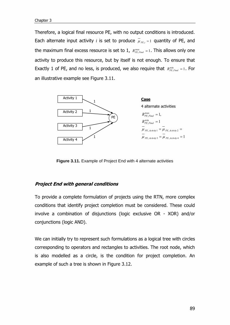
Chapter 3
89
Therefore, a logical final resource PE, with no output conditions is introduced.
Each alternate input activity i is set to produce 1, iPE quantity of PE, and
the maximum final excess resource is set to 1, 1max
, FinalPER . This allows only one
activity to produce this resource, but by itself is not enough. To ensure that
Exactly 1 of PE, and no less, is produced, we also require that 1min
, FinalPER . For
an illustrative example see Figure 3.11.
Figure 3.11. Example of Project End with 4 alternate activities
Project End with general conditions
To provide a complete formulation of projects using the RTN, more complex
conditions that identify project completion must be considered. These could
involve a combination of disjunctions (logic exclusive OR - XOR) and/or
conjunctions (logic AND).
We can initially try to represent such formulations as a logical tree with circles
corresponding to operators and rectangles to activities. The root node, which
is also modelled as a circle, is the condition for project completion. An
example of such a tree is shown in Figure 3.12.
Activity 3
PE
Activity 1
Activity 4
Activity 2
1
1
1
1
Case
4 alternate activities
1
1
,1
4,3,
2,1,
min
,
max
,
ActivityPEActivityPE
ActivityPEActivityPE
FinalPE
FinalPE
R
R
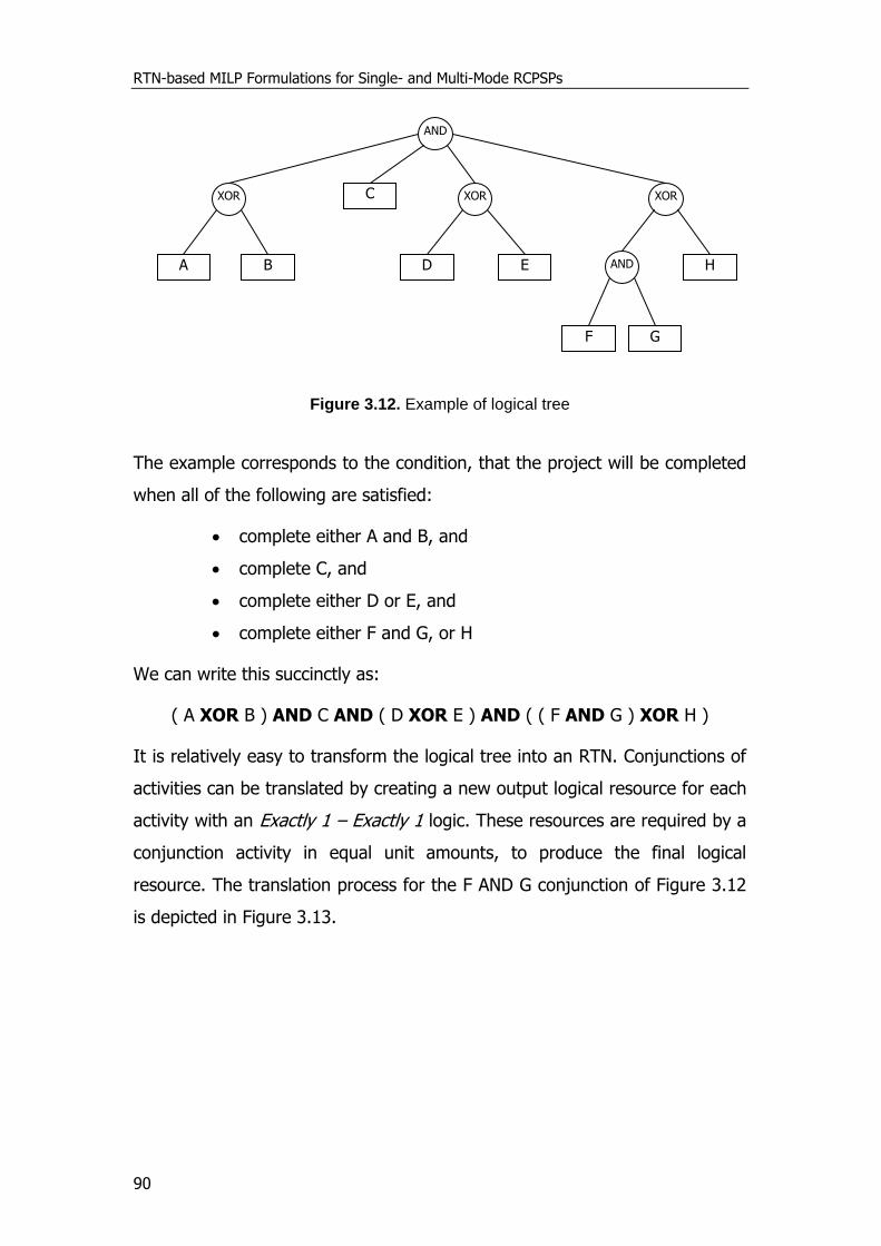
RTN-based MILP Formulations for Single- and Multi-Mode RCPSPs
90
Figure 3.12. Example of logical tree
The example corresponds to the condition, that the project will be completed
when all of the following are satisfied:
complete either A and B, and
complete C, and
complete either D or E, and
complete either F and G, or H
We can write this succinctly as:
( A XOR B ) AND C AND ( D XOR E ) AND ( ( F AND G ) XOR H )
It is relatively easy to transform the logical tree into an RTN. Conjunctions of
activities can be translated by creating a new output logical resource for each
activity with an Exactly 1 – Exactly 1 logic. These resources are required by a
conjunction activity in equal unit amounts, to produce the final logical
resource. The translation process for the F AND G conjunction of Figure 3.12
is depicted in Figure 3.13.
AND
A
XOR XOR XOR
B
C
D
E
H
F
G
AND
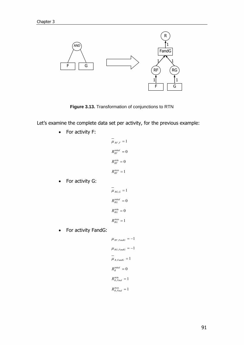
Chapter 3
91
Figure 3.13. Transformation of conjunctions to RTN
Let’s examine the complete data set per activity, for the previous example:
For activity F:
1, FRF
0initial
RFR
0min RFR
1max RFR
For activity G:
1, GRG
0initial
RGR
0min RGR
1max RGR
For activity FandG:
1, FandGRF
1, FandGRG
1, FandGR
0initial
RR
1min
, FinalRR
1max
, FinalRR
F
G
AND
FandG
R
RF RG
G
F
1 1
1 1
1
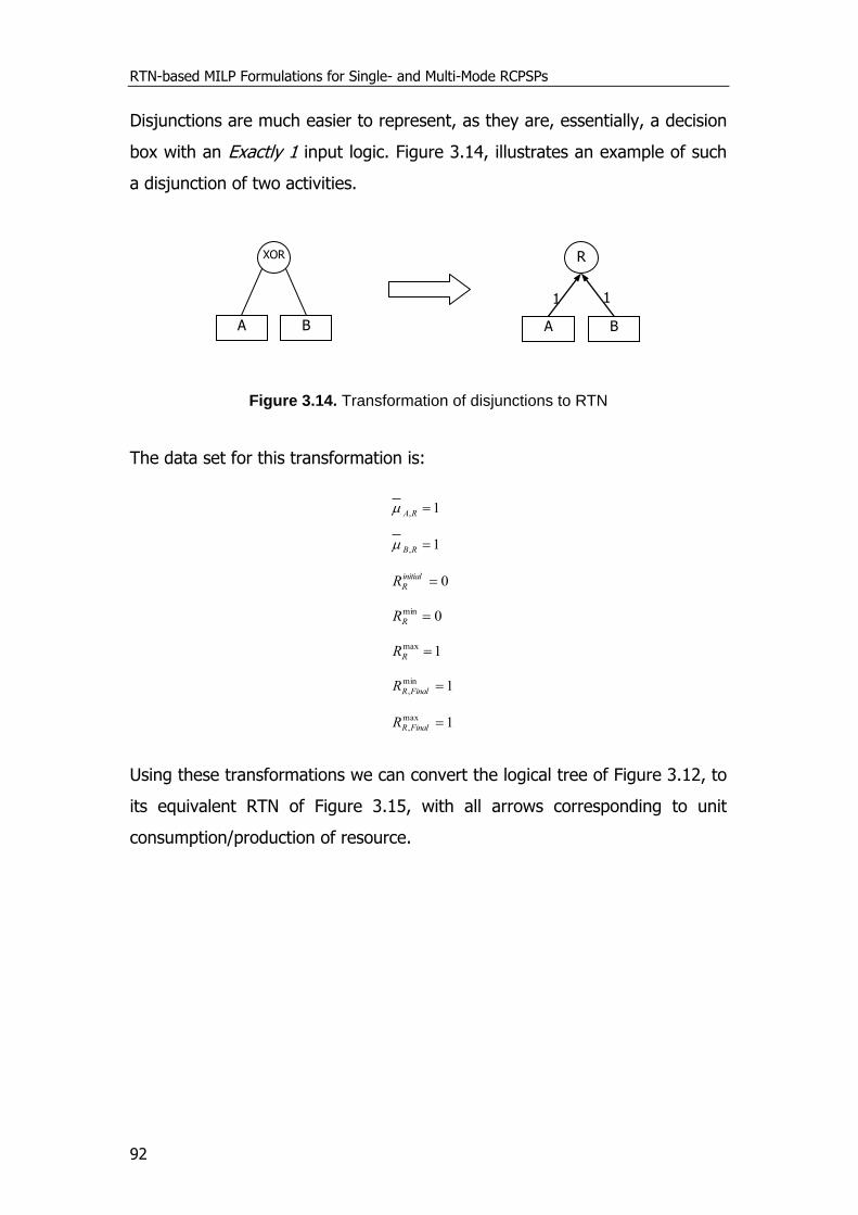
RTN-based MILP Formulations for Single- and Multi-Mode RCPSPs
92
Disjunctions are much easier to represent, as they are, essentially, a decision
box with an Exactly 1 input logic. Figure 3.14, illustrates an example of such
a disjunction of two activities.
Figure 3.14. Transformation of disjunctions to RTN
The data set for this transformation is:
1, RA
1, RB
0initial
RR
0min RR
1max RR
1min
, FinalRR
1max
, FinalRR
Using these transformations we can convert the logical tree of Figure 3.12, to
its equivalent RTN of Figure 3.15, with all arrows corresponding to unit
consumption/production of resource.
A
B
XOR R
B
A
1 1
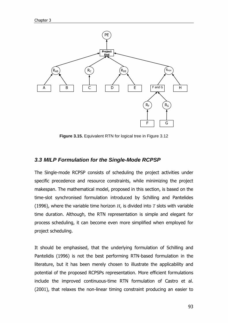
Chapter 3
93
Figure 3.15. Equivalent RTN for logical tree in Figure 3.12
3.3 MILP Formulation for the Single-Mode RCPSP
The Single-mode RCPSP consists of scheduling the project activities under
specific precedence and resource constraints, while minimizing the project
makespan. The mathematical model, proposed in this section, is based on the
time-slot synchronised formulation introduced by Schilling and Pantelides
(1996), where the variable time horizon H, is divided into T slots with variable
time duration. Although, the RTN representation is simple and elegant for
process scheduling, it can become even more simplified when employed for
project scheduling.
It should be emphasised, that the underlying formulation of Schilling and
Pantelidis (1996) is not the best performing RTN-based formulation in the
literature, but it has been merely chosen to illustrate the applicability and
potential of the proposed RCPSPs representation. More efficient formulations
include the improved continuous-time RTN formulation of Castro et al.
(2001), that relaxes the non-linear timing constraint producing an easier to
Project End
A
RAB RDE RFGH
B
C
D
E
H
F
G
F and G
RC
PE
RF RG
RTN-based MILP Formulations for Single- and Multi-Mode RCPSPs
94
solve, pure MILP problem and also the work of Castro et al. (2004), where a
new set of timing constraints further reduces the computational cost. The
main objective of this section is to establish a new modelling framework for
RCPSPs utilising techniques from the process scheduling area. The
representation of RCPSPs could provide the basis for translations into more
efficient RTN formulations than the original work of Schilling and Pantelidis
(1996).
The complete list of the notation used throughout this chapter is given in
Section 3.7. We set the number of time slots T equal to the number of
activities, in case the worst scenario is realised, with only one activity
executed at each slot. We assume that no more than one instance of an
activity can be executed at any time point. This assumption converts the
original RTN variable Nit, representing the number of activity instances
starting at time t, from integer to binary, since the only possible values are 0
and 1, depending on whether none or one instance of the activity is being
executed.
Additionally, resource consumption and production does not depend on the
size of the activity, so the corresponding size-dependent coefficients’ values
are 0, 0 riri vv .
Activities can be executed only once over the duration of the project. If an
activity is to be executed again, we represent it as a new one. This is because
it is bound to have different constraints, or else it would be included in the
first one, requiring double input and producing double output resources.
3.3.1 Constraints
Schilling and Pantelides (1996) distinguish four types of constraints: timing,
slot, excess resource balances and excess resource capacity constraints. We
will adapt these constraints to project scheduling problems.
Chapter 3
95
Two binary variables ity and ity are defined to express starting time and
spanning over consecutive time slots. The first set of binary variables ity ,
replace the RTN variable Nit and take a value of 1 if activity i starts at t or 0
otherwise. The second new variable ity , takes a value of 1 if activity i is
active over both t and t-1 or 0 otherwise. The model can be simplified by
setting 01,
iy , since no task can be active over t = 0, as it is out of the
scheduling horizon. Using the ity variable (activity spanning over two
adjacent slots), instead of tity (activity spanning over multiple slots) used in
the original RTN, results in a simpler mathematical model with far fewer
binary variables than the original one.
Timing Constraints
The total duration of all time slots t must be equal to the time horizon H:
T
t
t H1
(1)
A project activity i may extend over one or more consecutive time slots and
the sum of the durations of these slots must be equal to the duration θi of the
activity. Using the new variables ity and ity , instead of itN and tity the
timing constraints of the general RTN formulation (Schilling and Pantelides,
1996) are transformed to:
iyyyT
t
it
T
t
ititit
,11
(2)
We note that constraint (2) involves nonlinearities since both the binary
variables ity and ity and the slot durations t are variables. These
nonlinearities can be removed using standard techniques (Glover, 1975).
Considering that at most one instance of task i can be active at any time, we
RTN-based MILP Formulations for Single- and Multi-Mode RCPSPs
96
define the new variables tititit yylin . This definition can be effected
using the following linear constraints:
tiyylinyyititiititit ,,,min maxmin (3)
tilinyy titititt ,,1max (4)
where min and max are the minimum and maximum slot durations,
respectively. We can set the maximum slot duration to be equal to the value
of the greatest activity duration max
i and the minimum duration equal to 1.
After applying this linearization technique, constraint (2) becomes linear:
iylinT
t
it
T
t
iit
,11
(5)
Slot Constraints
Variable 1, tiy can take a value of 1 only if activity i started at an earlier time
slot ( 1 t ) and is still active over 1t . For an activity to start at an earlier
time one of the variables ity or ity must take a value of 1. To ensure proper
activity execution over multiple time slots we now need both new variables
ity and ity , instead of tity and this is expressed as:
1,1,,1,
Ttiyyytiitit (6)
If activity i has not been active over slot t, the value of all three variables
must be 0. The inequality is necessary for the case that activity i is actually
completed at the end of slot t. The possible combinations for the values of
the previous variables are shown on Table 3.2.
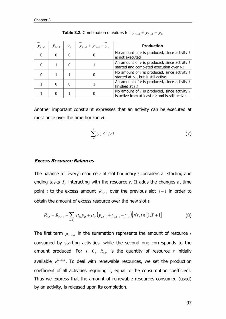
Chapter 3
97
Table 3.2. Combination of values for ittitiyyy 1,1,
1, tiy 1, tiy
ity ittiti yyy 1,1, Production
0 0 0 0 No amount of r is produced, since activity i
is not executed
0 1 0 1 An amount of r is produced, since activity i
started and completed execution over t-1
0 1 1 0 No amount of r is produced, since activity i
started at t-1, but is still active.
1 0 0 1 An amount of r is produced, since activity i
finished at t-1
1 0 1 0 No amount of r is produced, since activity i
is active from at least t-2 and is still active
Another important constraint expresses that an activity can be executed at
most once over the time horizon H:
iyT
t
it
,11
(7)
Excess Resource Balances
The balance for every resource r at slot boundary t considers all starting and
ending tasks rI interacting with the resource r. It adds the changes at time
point t to the excess amount 1, trR over the previous slot 1t in order to
obtain the amount of excess resource over the new slot t:
1,1,,1,1,1,,
TtryyyyRRrIi
ittitiriitritrtr (8)
The first term itri y in the summation represents the amount of resource r
consumed by starting activities, while the second one corresponds to the
amount produced. For 0t , 0,rR is the quantity of resource r initially
available initial
rR . To deal with renewable resources, we set the production
coefficient of all activities requiring it, equal to the consumption coefficient.
Thus we express that the amount of renewable resources consumed (used)
by an activity, is released upon its completion.
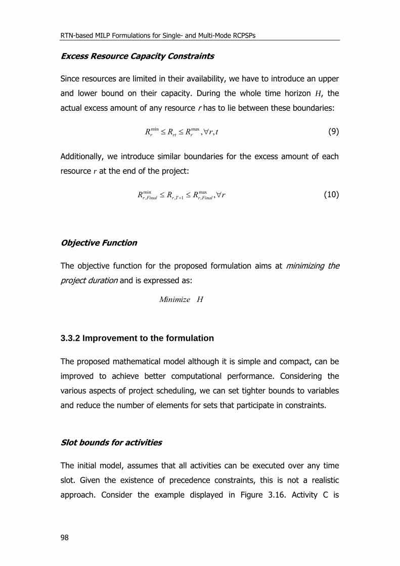
RTN-based MILP Formulations for Single- and Multi-Mode RCPSPs
98
Excess Resource Capacity Constraints
Since resources are limited in their availability, we have to introduce an upper
and lower bound on their capacity. During the whole time horizon H, the
actual excess amount of any resource r has to lie between these boundaries:
trRRR rrtr ,,maxmin (9)
Additionally, we introduce similar boundaries for the excess amount of each
resource r at the end of the project:
rRRR FinalrTrFinalr ,max
,1,
min
, (10)
Objective Function
The objective function for the proposed formulation aims at minimizing the
project duration and is expressed as:
HMinimize
3.3.2 Improvement to the formulation
The proposed mathematical model although it is simple and compact, can be
improved to achieve better computational performance. Considering the
various aspects of project scheduling, we can set tighter bounds to variables
and reduce the number of elements for sets that participate in constraints.
Slot bounds for activities
The initial model, assumes that all activities can be executed over any time
slot. Given the existence of precedence constraints, this is not a realistic
approach. Consider the example displayed in Figure 3.16. Activity C is
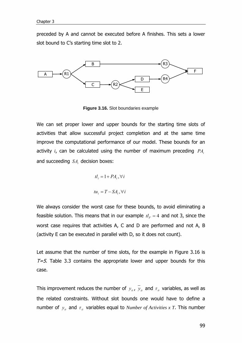
Chapter 3
99
preceded by A and cannot be executed before A finishes. This sets a lower
slot bound to C’s starting time slot to 2.
Figure 3.16. Slot boundaries example
We can set proper lower and upper bounds for the starting time slots of
activities that allow successful project completion and at the same time
improve the computational performance of our model. These bounds for an
activity i, can be calculated using the number of maximum preceding iPA
and succeeding iSA decision boxes:
iPAtl ii ,1
iSATtu ii ,
We always consider the worst case for these bounds, to avoid eliminating a
feasible solution. This means that in our example 4Ftl and not 3, since the
worst case requires that activities A, C and D are performed and not A, B
(activity E can be executed in parallel with D, so it does not count).
Let assume that the number of time slots, for the example in Figure 3.16 is
T=5. Table 3.3 contains the appropriate lower and upper bounds for this
case.
This improvement reduces the number of ity , ity and it variables, as well as
the related constraints. Without slot bounds one would have to define a
number of ity and it variables equal to Number of Activities x T. This number
B
R1
R3
A
C
R2
D
E
R4
F
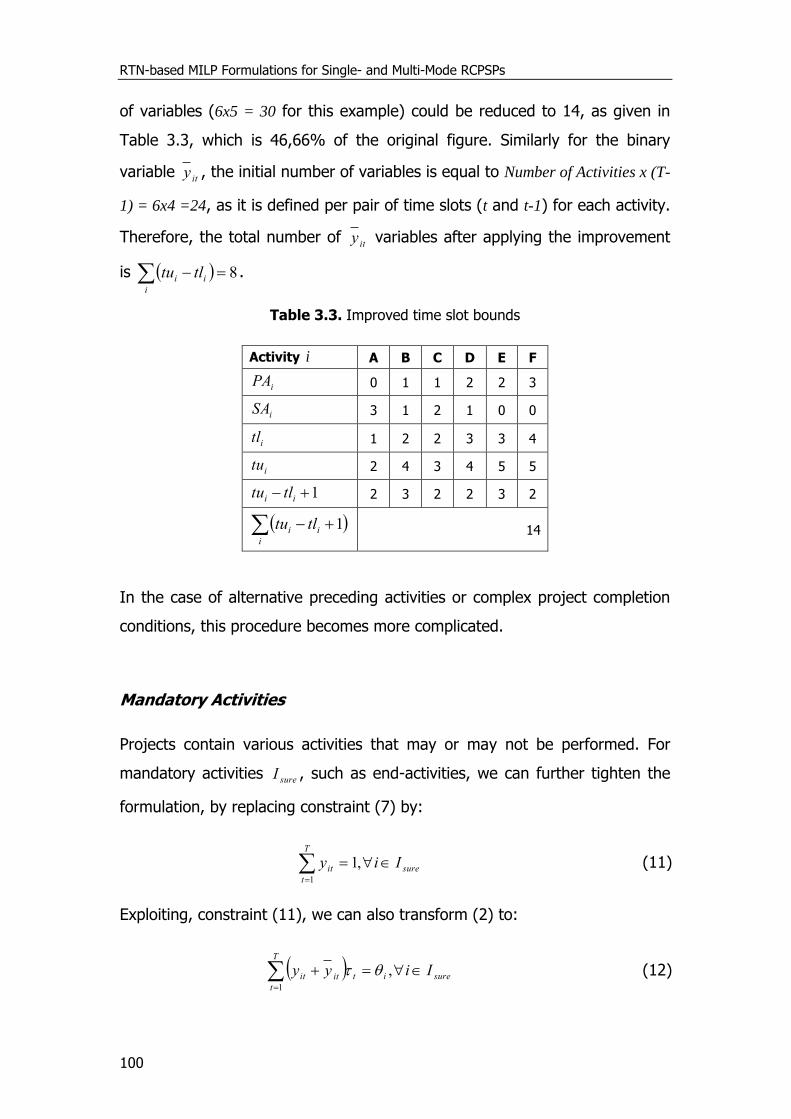
RTN-based MILP Formulations for Single- and Multi-Mode RCPSPs
100
of variables (6x5 = 30 for this example) could be reduced to 14, as given in
Table 3.3, which is 46,66% of the original figure. Similarly for the binary
variable ity , the initial number of variables is equal to Number of Activities x (T-
1) = 6x4 =24, as it is defined per pair of time slots (t and t-1) for each activity.
Therefore, the total number of ity variables after applying the improvement
is i
ii tltu 8 .
Table 3.3. Improved time slot bounds
Activity i A B C D E F
iPA 0 1 1 2 2 3
iSA 3 1 2 1 0 0
itl 1 2 2 3 3 4
itu 2 4 3 4 5 5
1 ii tltu 2 3 2 2 3 2
i
ii tltu 1 14
In the case of alternative preceding activities or complex project completion
conditions, this procedure becomes more complicated.
Mandatory Activities
Projects contain various activities that may or may not be performed. For
mandatory activities sureI , such as end-activities, we can further tighten the
formulation, by replacing constraint (7) by:
sure
T
t
it Iiy
,11
(11)
Exploiting, constraint (11), we can also transform (2) to:
sure
T
t
ititit Iiyy
,1
(12)
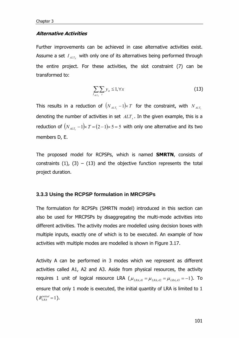
Chapter 3
101
Alternative Activities
Further improvements can be achieved in case alternative activities exist.
Assume a set XALTI with only one of its alternatives being performed through
the entire project. For these activities, the slot constraint (7) can be
transformed to:
xy
xALTI t
it ,1 (13)
This results in a reduction of TNxALT 1 for the constraint, with
xALTN
denoting the number of activities in set xALT . In the given example, this is a
reduction of 55121 TNxALT
with only one alternative and its two
members D, E.
The proposed model for RCPSPs, which is named SMRTN, consists of
constraints (1), (3) – (13) and the objective function represents the total
project duration.
3.3.3 Using the RCPSP formulation in MRCPSPs
The formulation for RCPSPs (SMRTN model) introduced in this section can
also be used for MRCPSPs by disaggregating the multi-mode activities into
different activities. The activity modes are modelled using decision boxes with
multiple inputs, exactly one of which is to be executed. An example of how
activities with multiple modes are modelled is shown in Figure 3.17.
Activity A can be performed in 3 modes which we represent as different
activities called A1, A2 and A3. Aside from physical resources, the activity
requires 1 unit of logical resource LRA ( 13,2,1, ALRAALRAALRA ). To
ensure that only 1 mode is executed, the initial quantity of LRA is limited to 1
( 1initial
LRAR ).
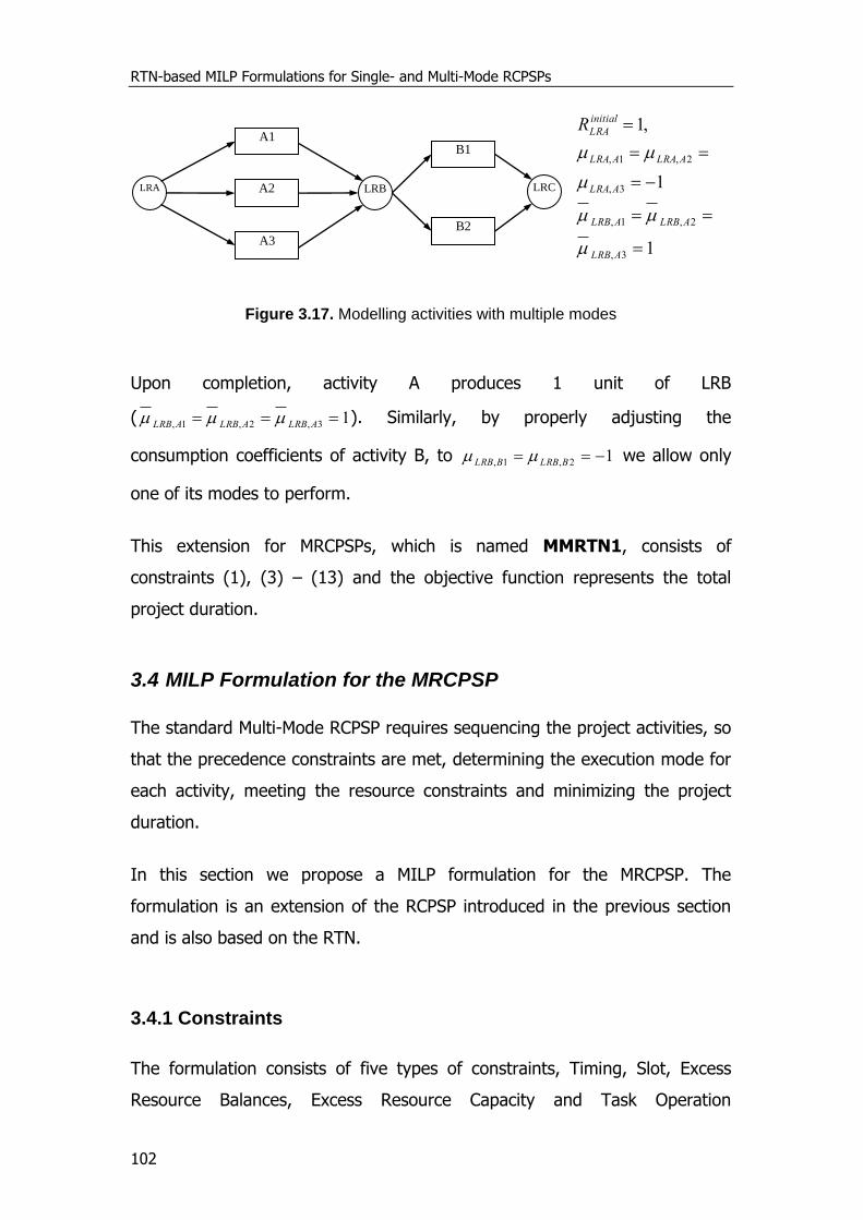
RTN-based MILP Formulations for Single- and Multi-Mode RCPSPs
102
Figure 3.17. Modelling activities with multiple modes
Upon completion, activity A produces 1 unit of LRB
( 13,2,1, ALRBALRBALRB ). Similarly, by properly adjusting the
consumption coefficients of activity B, to 12,1, BLRBBLRB we allow only
one of its modes to perform.
This extension for MRCPSPs, which is named MMRTN1, consists of
constraints (1), (3) – (13) and the objective function represents the total
project duration.
3.4 MILP Formulation for the MRCPSP
The standard Multi-Mode RCPSP requires sequencing the project activities, so
that the precedence constraints are met, determining the execution mode for
each activity, meeting the resource constraints and minimizing the project
duration.
In this section we propose a MILP formulation for the MRCPSP. The
formulation is an extension of the RCPSP introduced in the previous section
and is also based on the RTN.
3.4.1 Constraints
The formulation consists of five types of constraints, Timing, Slot, Excess
Resource Balances, Excess Resource Capacity and Task Operation
1
1
,1
3,
2,1,
3,
2,1,
ALRB
ALRBALRB
ALRA
ALRAALRA
initial
LRAR
A3
A1
A2
B2
LRB
B1
LRA LRC
Chapter 3
103
constraints. As in the RCPSP formulation, we can simplify the model, by
setting 01,
iy , since no task can be active over 0t .
Timing Constraints
The total duration of all time slots must be equal to the time horizon:
T
t
t H1
(14)
A project activity i may extend over one or more consecutive time slots and
the sum of the durations of these slots must be equal to the duration mi of
activity i in mode m:
izyym
mimi
T
t
titit
,1
(15)
Where miz is a binary variable that expresses whether alternate mode m of
activity i is chosen (1) or not (0).
The linearization of the left of constraint (15) can be performed as described
in Section 3.3.1 We define new variables tititit yylin , through the
linear constraints:
tiyylinyyititmiititit ,,)max(,min maxmin (16)
tilinyy titititt ,,1max (17)
where τmin and τ
max are the minimum and maximum slot durations,
respectively. We can set the maximum slot duration to be equal to the value
of the greatest activity duration max
mi . After applying this linearization
technique, constraint (15) becomes linear:
RTN-based MILP Formulations for Single- and Multi-Mode RCPSPs
104
izlinT
t m
mimiit
,1
(18)
Slot Constraints
As in the RCPSP formulation, variable 1, tiy can take a value of 1 only if
activity i started at an earlier time slot ( 1 t ) and is still active over 1t .
For an activity to start at an earlier time one of the variables ity or ity must
take a value of 1. These constraints can be combined to the following
inequality:
1,1,,1,
Ttiyyytiitit (19)
If activity i has not been active over slot t, the value of all three variables
must be 0. The inequality is necessary for the case that activity i is actually
completed at the end of slot t.
An activity can be executed at most once over the time horizon H:
iyT
t
it
,11
(20)
and if so, only one activity mode is performed:
iyzT
t
it
m
mi
,1
(21)
Excess Resource Balances
The balance of a resource r at slot boundary t is given by:
tryyySSySSRRrIi
ittitiri
L
riitri
L
ritrtr ,,1,1,1,,
(22)
Chapter 3
105
The ri and ri coefficients of the RCPSP formulation, are now replaced by
the minimum resource consumption and production values L
riS and L
riS plus
their surplus variables riS and riS respectively.
The values of U
ri
L
ri SS coefficients representing the minimum/maximum
quantities of resource r required by the various modes m at the beginning of
activity i, are given by:
imr
L
ri aS min and imr
U
ri aS max
Similarly, the values of the minimum/maximum quantities of resource r
produced by the various modes m at the end of activity i, U
ri
L
ri SS are given
by:
imr
L
ri aS min and imr
U
ri aS max
Surplus variables riS and riS depend on the selected mode m, are bounded
by constraints (30) and (31) and calculated through (32) and (33), as
presented in the Task Operation Constraints section below.
The excess resource balance contains a type of nonlinearities similar to
constraint (15), which can be removed by introducing two new variables:
riitrit SyS and riittitirit SyyyS 1,1,
The first variable ritS is defined:
)(,,0 ritySSS it
L
ri
U
ririt (23)
)(, riSS ri
t
rit (24)
Similarly for the second variable ritS :
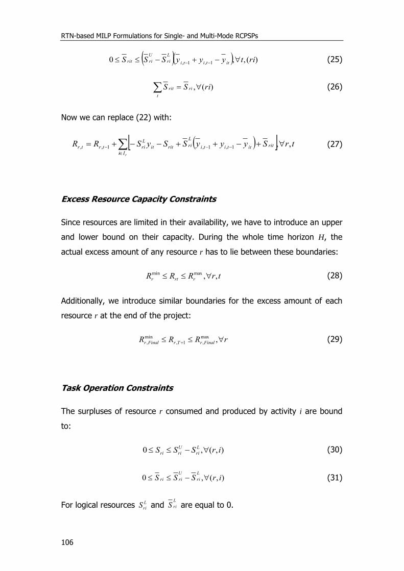
RTN-based MILP Formulations for Single- and Multi-Mode RCPSPs
106
)(,,0 1,1,rityyySSS
ittiti
L
ri
U
ririt (25)
)(, riSS ri
t
rit (26)
Now we can replace (22) with:
trSyyySSySRRrIi
ritittiti
L
riritit
L
ritrtr ,,1,1,1,,
(27)
Excess Resource Capacity Constraints
Since resources are limited in their availability, we have to introduce an upper
and lower bound on their capacity. During the whole time horizon H, the
actual excess amount of any resource r has to lie between these boundaries:
trRRR rrtr ,,maxmin (28)
Additionally, we introduce similar boundaries for the excess amount of each
resource r at the end of the project:
rRRR FinalrTrFinalr ,max
,1,
min
, (29)
Task Operation Constraints
The surpluses of resource r consumed and produced by activity i are bound
to:
),(,0 irSSS L
ri
U
riri (30)
),(,0 irSSSL
ri
U
riri (31)
For logical resources L
riS and L
riS are equal to 0.
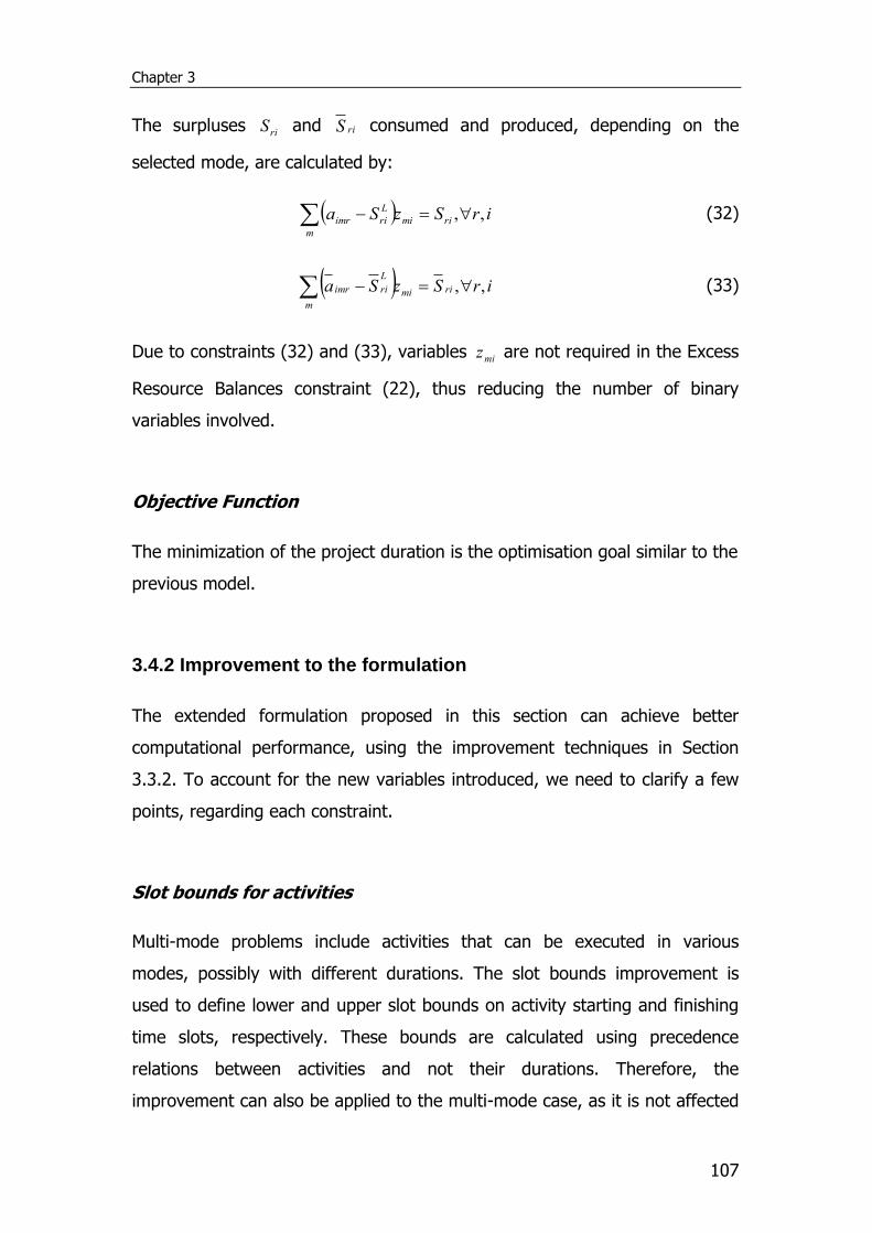
Chapter 3
107
The surpluses riS and riS consumed and produced, depending on the
selected mode, are calculated by:
irSzSa rimi
m
L
riimr ,, (32)
irSzSa rimi
m
L
riimr ,, (33)
Due to constraints (32) and (33), variables miz are not required in the Excess
Resource Balances constraint (22), thus reducing the number of binary
variables involved.
Objective Function
The minimization of the project duration is the optimisation goal similar to the
previous model.
3.4.2 Improvement to the formulation
The extended formulation proposed in this section can achieve better
computational performance, using the improvement techniques in Section
3.3.2. To account for the new variables introduced, we need to clarify a few
points, regarding each constraint.
Slot bounds for activities
Multi-mode problems include activities that can be executed in various
modes, possibly with different durations. The slot bounds improvement is
used to define lower and upper slot bounds on activity starting and finishing
time slots, respectively. These bounds are calculated using precedence
relations between activities and not their durations. Therefore, the
improvement can also be applied to the multi-mode case, as it is not affected
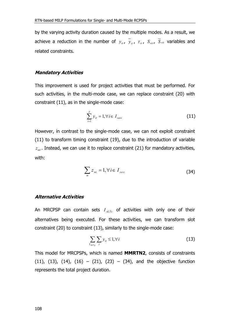
RTN-based MILP Formulations for Single- and Multi-Mode RCPSPs
108
by the varying activity duration caused by the multiple modes. As a result, we
achieve a reduction in the number of ity , ity , it , ritS , ritS variables and
related constraints.
Mandatory Activities
This improvement is used for project activities that must be performed. For
such activities, in the multi-mode case, we can replace constraint (20) with
constraint (11), as in the single-mode case:
sure
T
t
it Iiy
,11
(11)
However, in contrast to the single-mode case, we can not exploit constraint
(11) to transform timing constraint (19), due to the introduction of variable
miz . Instead, we can use it to replace constraint (21) for mandatory activities,
with:
sure
m
miIiz ,1 (34)
Alternative Activities
An MRCPSP can contain sets ALTxI of activities with only one of their
alternatives being executed. For these activities, we can transform slot
constraint (20) to constraint (13), similarly to the single-mode case:
iy
XALT t
it ,1I
(13)
This model for MRCPSPs, which is named MMRTN2, consists of constraints
(11), (13), (14), (16) – (21), (23) – (34), and the objective function
represents the total project duration.
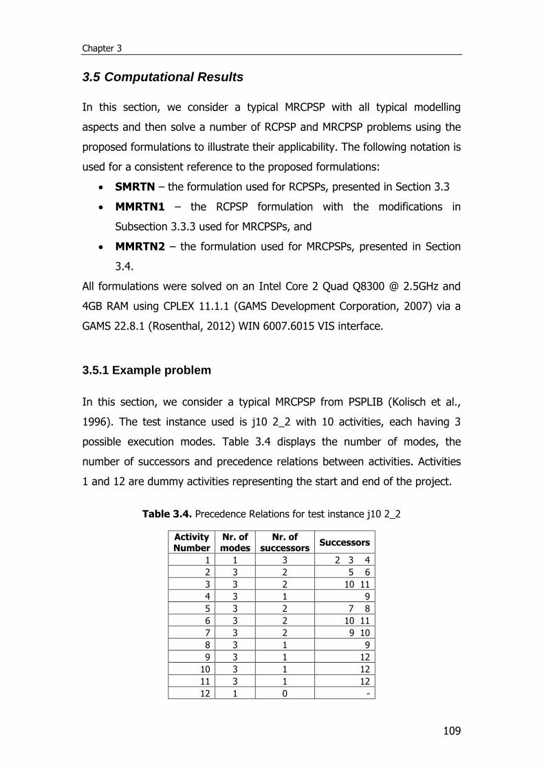
Chapter 3
109
3.5 Computational Results
In this section, we consider a typical MRCPSP with all typical modelling
aspects and then solve a number of RCPSP and MRCPSP problems using the
proposed formulations to illustrate their applicability. The following notation is
used for a consistent reference to the proposed formulations:
SMRTN – the formulation used for RCPSPs, presented in Section 3.3
MMRTN1 – the RCPSP formulation with the modifications in
Subsection 3.3.3 used for MRCPSPs, and
MMRTN2 – the formulation used for MRCPSPs, presented in Section
3.4.
All formulations were solved on an Intel Core 2 Quad Q8300 @ 2.5GHz and
4GB RAM using CPLEX 11.1.1 (GAMS Development Corporation, 2007) via a
GAMS 22.8.1 (Rosenthal, 2012) WIN 6007.6015 VIS interface.
3.5.1 Example problem
In this section, we consider a typical MRCPSP from PSPLIB (Kolisch et al.,
1996). The test instance used is j10 2_2 with 10 activities, each having 3
possible execution modes. Table 3.4 displays the number of modes, the
number of successors and precedence relations between activities. Activities
1 and 12 are dummy activities representing the start and end of the project.
Table 3.4. Precedence Relations for test instance j10 2_2
Activity Number
Nr. of modes
Nr. of successors
Successors
1 1 3 2 3 4
2 3 2 5 6
3 3 2 10 11
4 3 1 9
5 3 2 7 8
6 3 2 10 11
7 3 2 9 10
8 3 1 9
9 3 1 12
10 3 1 12
11 3 1 12
12 1 0 -
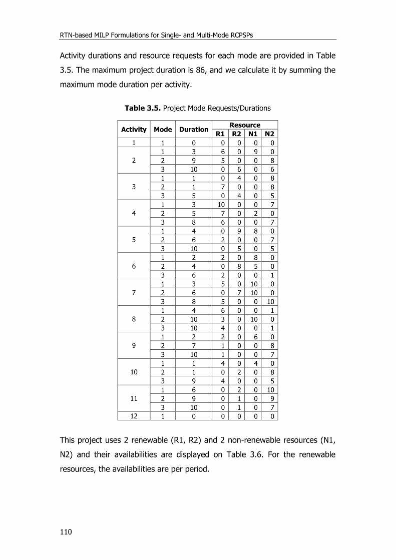
RTN-based MILP Formulations for Single- and Multi-Mode RCPSPs
110
Activity durations and resource requests for each mode are provided in Table
3.5. The maximum project duration is 86, and we calculate it by summing the
maximum mode duration per activity.
Table 3.5. Project Mode Requests/Durations
Activity Mode Duration Resource
R1 R2 N1 N2
1 1 0 0 0 0 0
2
1 3 6 0 9 0
2 9 5 0 0 8
3 10 0 6 0 6
3
1 1 0 4 0 8
2 1 7 0 0 8
3 5 0 4 0 5
4
1 3 10 0 0 7
2 5 7 0 2 0
3 8 6 0 0 7
5
1 4 0 9 8 0
2 6 2 0 0 7
3 10 0 5 0 5
6
1 2 2 0 8 0
2 4 0 8 5 0
3 6 2 0 0 1
7
1 3 5 0 10 0
2 6 0 7 10 0
3 8 5 0 0 10
8
1 4 6 0 0 1
2 10 3 0 10 0
3 10 4 0 0 1
9
1 2 2 0 6 0
2 7 1 0 0 8
3 10 1 0 0 7
10
1 1 4 0 4 0
2 1 0 2 0 8
3 9 4 0 0 5
11
1 6 0 2 0 10
2 9 0 1 0 9
3 10 0 1 0 7
12 1 0 0 0 0 0
This project uses 2 renewable (R1, R2) and 2 non-renewable resources (N1,
N2) and their availabilities are displayed on Table 3.6. For the renewable
resources, the availabilities are per period.
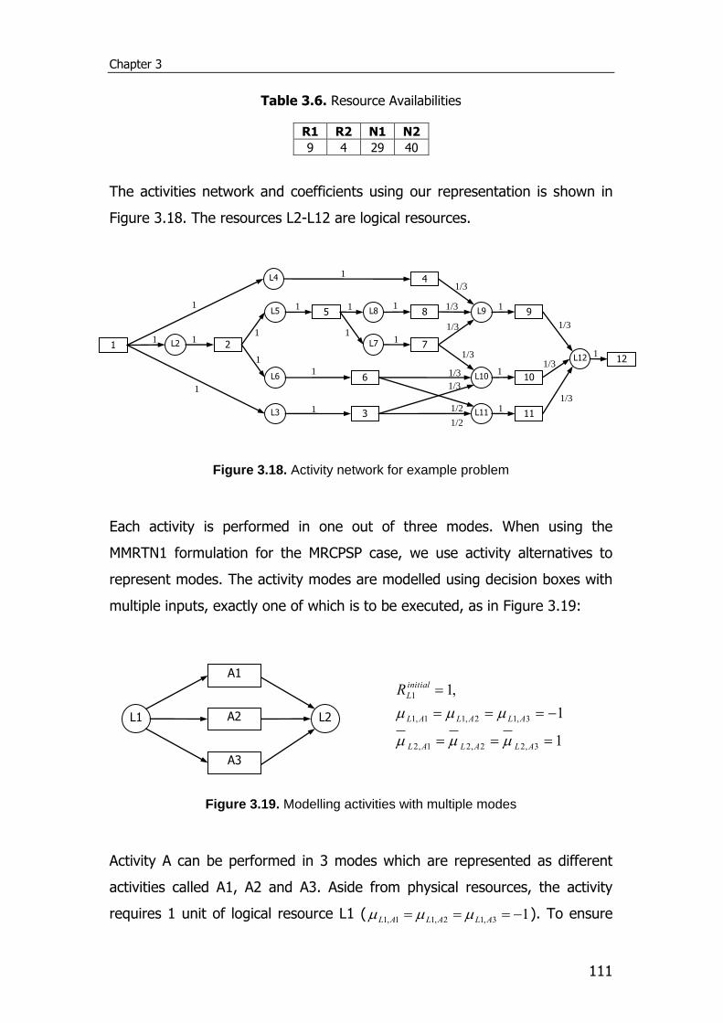
Chapter 3
111
Table 3.6. Resource Availabilities
R1 R2 N1 N2
9 4 29 40
The activities network and coefficients using our representation is shown in
Figure 3.18. The resources L2-L12 are logical resources.
Figure 3.18. Activity network for example problem
Each activity is performed in one out of three modes. When using the
MMRTN1 formulation for the MRCPSP case, we use activity alternatives to
represent modes. The activity modes are modelled using decision boxes with
multiple inputs, exactly one of which is to be executed, as in Figure 3.19:
Figure 3.19. Modelling activities with multiple modes
Activity A can be performed in 3 modes which are represented as different
activities called A1, A2 and A3. Aside from physical resources, the activity
requires 1 unit of logical resource L1 ( 13,12,11,1 ALALAL ). To ensure
1
1
,1
3,22,21,2
3,12,11,1
1
ALALAL
ALALAL
initial
LR
A3
A1
A2
L2 L1
1
4
8
7
L9
L4
5 L8
L7
L10
9
10
11 L11
6
2
L5
L6
3
L2
L3
L12 12
1
1/3
1/2
1 1
1
1
1
1
1
1
1 1/2
1/3
1/3
1
1
1
1
1
1
1
1/3
1/3
1/3 1/3
1/3
1/3 1
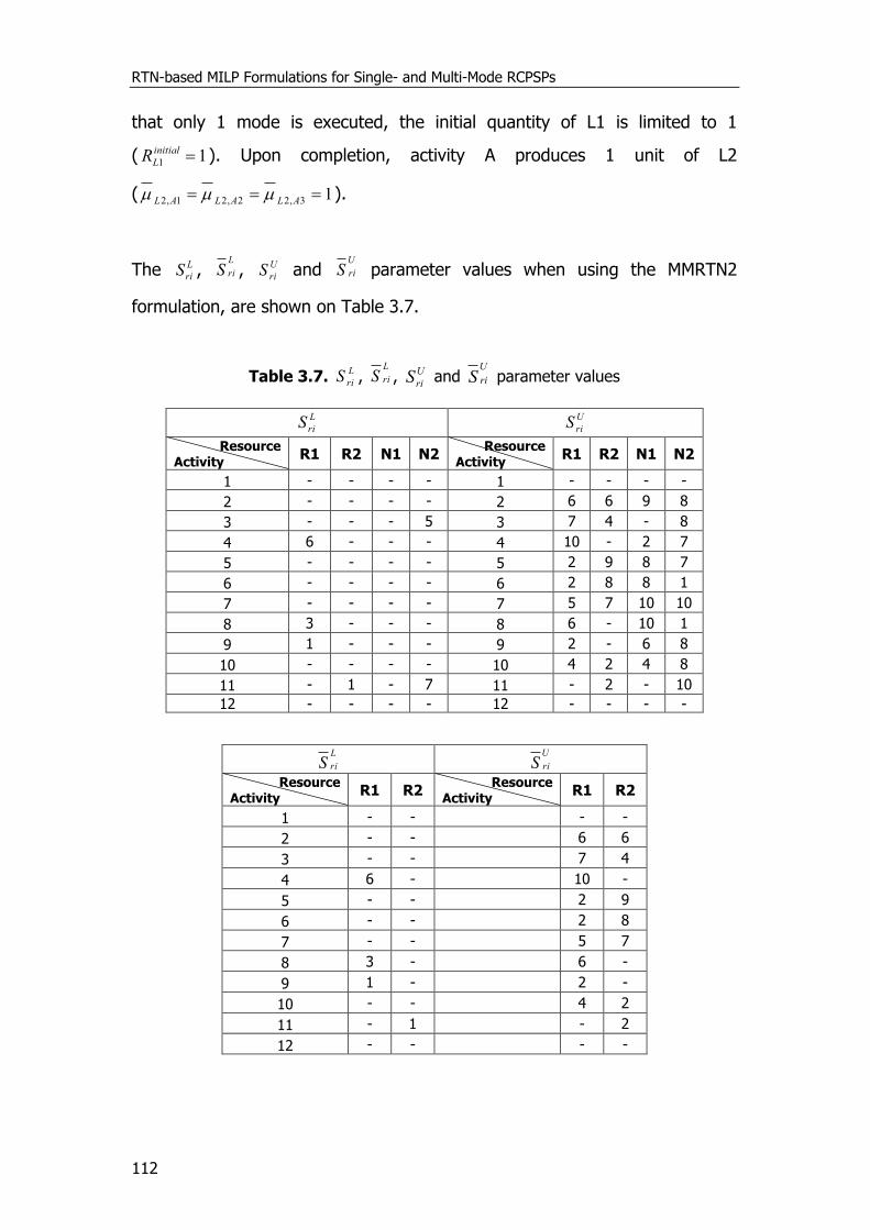
RTN-based MILP Formulations for Single- and Multi-Mode RCPSPs
112
that only 1 mode is executed, the initial quantity of L1 is limited to 1
( 11 initial
LR ). Upon completion, activity A produces 1 unit of L2
( 13,22,21,2 ALALAL ).
The L
riS , L
riS , U
riS and U
riS parameter values when using the MMRTN2
formulation, are shown on Table 3.7.
Table 3.7. L
riS , L
riS , U
riS and U
riS parameter values
L
riS U
riS
Resource Activity
R1 R2 N1 N2 Resource
Activity R1 R2 N1 N2
1 - - - - 1 - - - -
2 - - - - 2 6 6 9 8
3 - - - 5 3 7 4 - 8
4 6 - - - 4 10 - 2 7
5 - - - - 5 2 9 8 7
6 - - - - 6 2 8 8 1
7 - - - - 7 5 7 10 10
8 3 - - - 8 6 - 10 1
9 1 - - - 9 2 - 6 8
10 - - - - 10 4 2 4 8
11 - 1 - 7 11 - 2 - 10
12 - - - - 12 - - - -
L
riS U
riS
Resource Activity
R1 R2 Resource
Activity R1 R2
1 - - - -
2 - - 6 6
3 - - 7 4
4 6 - 10 -
5 - - 2 9
6 - - 2 8
7 - - 5 7
8 3 - 6 -
9 1 - 2 -
10 - - 4 2
11 - 1 - 2
12 - - - -
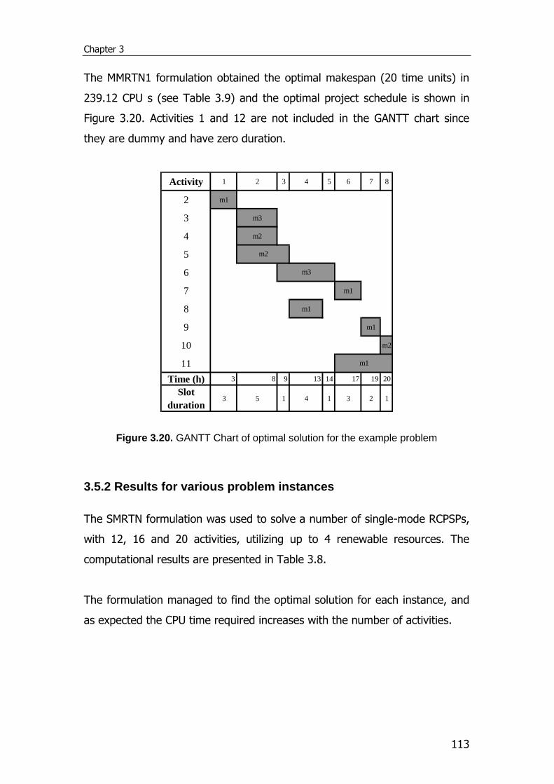
Chapter 3
113
The MMRTN1 formulation obtained the optimal makespan (20 time units) in
239.12 CPU s (see Table 3.9) and the optimal project schedule is shown in
Figure 3.20. Activities 1 and 12 are not included in the GANTT chart since
they are dummy and have zero duration.
Activity 1 2 3 4 5 6 7 8
2 m1
3 m3
4 m2
5
6
7 m1
8 m1
9 m1
10 m2
11
Time (h) 3 8 9 13 14 17 19 20
Slot
duration3 5 1 4 1 3 2 1
m2
m3
m1
Figure 3.20. GANTT Chart of optimal solution for the example problem
3.5.2 Results for various problem instances
The SMRTN formulation was used to solve a number of single-mode RCPSPs,
with 12, 16 and 20 activities, utilizing up to 4 renewable resources. The
computational results are presented in Table 3.8.
The formulation managed to find the optimal solution for each instance, and
as expected the CPU time required increases with the number of activities.
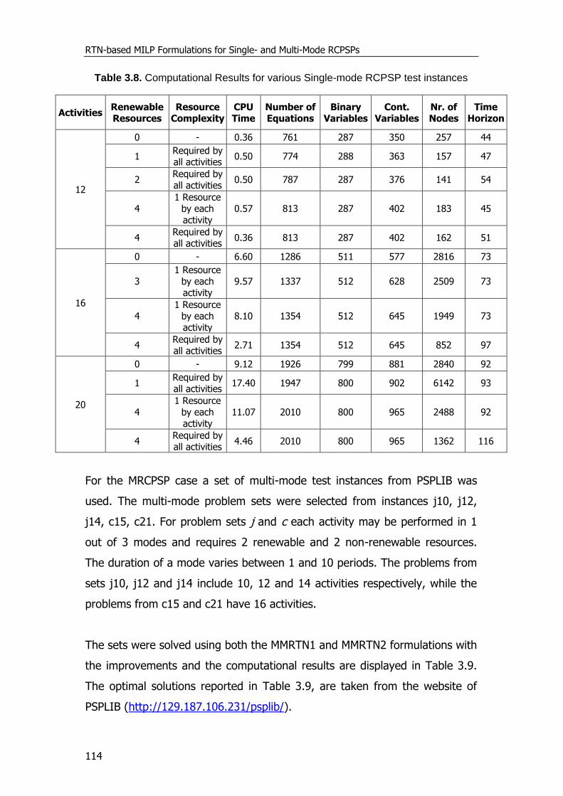
RTN-based MILP Formulations for Single- and Multi-Mode RCPSPs
114
Table 3.8. Computational Results for various Single-mode RCPSP test instances
Activities Renewable Resources
Resource Complexity
CPU Time
Number of Equations
Binary Variables
Cont. Variables
Nr. of Nodes
Time Horizon
12
0 - 0.36 761 287 350 257 44
1 Required by all activities
0.50 774 288 363 157 47
2 Required by all activities
0.50 787 287 376 141 54
4 1 Resource
by each activity
0.57 813 287 402 183 45
4 Required by all activities
0.36 813 287 402 162 51
16
0 - 6.60 1286 511 577 2816 73
3 1 Resource
by each activity
9.57 1337 512 628 2509 73
4 1 Resource
by each activity
8.10 1354 512 645 1949 73
4 Required by all activities
2.71 1354 512 645 852 97
20
0 - 9.12 1926 799 881 2840 92
1 Required by all activities
17.40 1947 800 902 6142 93
4 1 Resource
by each activity
11.07 2010 800 965 2488 92
4 Required by all activities
4.46 2010 800 965 1362 116
For the MRCPSP case a set of multi-mode test instances from PSPLIB was
used. The multi-mode problem sets were selected from instances j10, j12,
j14, c15, c21. For problem sets j and c each activity may be performed in 1
out of 3 modes and requires 2 renewable and 2 non-renewable resources.
The duration of a mode varies between 1 and 10 periods. The problems from
sets j10, j12 and j14 include 10, 12 and 14 activities respectively, while the
problems from c15 and c21 have 16 activities.
The sets were solved using both the MMRTN1 and MMRTN2 formulations with
the improvements and the computational results are displayed in Table 3.9.
The optimal solutions reported in Table 3.9, are taken from the website of
PSPLIB (http://129.187.106.231/psplib/).
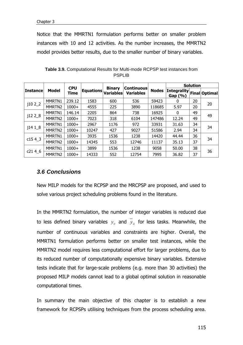
Chapter 3
115
Notice that the MMRTN1 formulation performs better on smaller problem
instances with 10 and 12 activities. As the number increases, the MMRTN2
model provides better results, due to the smaller number of binary variables.
Table 3.9. Computational Results for Multi-mode RCPSP test instances from
PSPLIB
Instance Model CPU Time
Equations Binary
Variables Continuous Variables
Nodes
Solution
Integrality Gap (%)
Final Optimal
j10 2_2 MMRTN1 239.12 1583 600 536 59423 0 20
20 MMRTN2 1000+ 4555 225 3890 118685 5.97 20
j12 2_8 MMRTN1 146.14 2205 864 738 16925 0 49
49 MMRTN2 1000+ 7023 318 6104 147486 12.24 49
j14 1_8 MMRTN1 1000+ 2967 1176 972 33931 31.63 34
34 MMRTN2 1000+ 10247 427 9027 51586 2.94 34
c15 4_3 MMRTN1 1000+ 3935 1536 1238 14420 44.44 36
34 MMRTN2 1000+ 14345 553 12746 11137 35.13 37
c21 4_6 MMRTN1 1000+ 3899 1536 1238 9058 50.00 38
36 MMRTN2 1000+ 14333 552 12754 7995 36.82 37
3.6 Conclusions
New MILP models for the RCPSP and the MRCPSP are proposed, and used to
solve various project scheduling problems found in the literature.
In the MMRTN2 formulation, the number of integer variables is reduced due
to less defined binary variables ity and ity for less tasks. Meanwhile, the
number of continuous variables and constraints are higher. Overall, the
MMRTN1 formulation performs better on smaller test instances, while the
MMRTN2 model requires less computational effort for larger problems, due to
its reduced number of computationally expensive binary variables. Extensive
tests indicate that for large-scale problems (e.g. more than 30 activities) the
proposed MILP models cannot lead to a global optimal solution in reasonable
computational times.
In summary the main objective of this chapter is to establish a new
framework for RCPSPs utilising techniques from the process scheduling area.
RTN-based MILP Formulations for Single- and Multi-Mode RCPSPs
116
As such, the proposed models are suitable to be integrated with challenging
process scheduling problems where project scheduling decisions are also
important (e.g. pharmaceutical product design and scheduling process). In
general the computational results and the similarities between process and
project scheduling problems, such as initial and target inventories, required
resource types and precedence relations, suggest that exchanging solution
techniques between the two research fields is both possible and useful.
3.7 Nomenclature
Indices/ Sets
Ii activities
Rr resources
Tt ,...,1 time slots
Subsets
XALTI xth set of alternative activities, 1 of which is to be executed,
IIXALT
rI activities interacting with resource r, II r
sureI activities that must be executed, II sure
Parameters
initial
rR initial available quantity of resource r
maxmin
rr RR minimum/maximum possible quantities for resource r
max
,
min
, FinalrFinalr RR minimum/maximum excess of resource r at the end of the
project
U
ri
L
ri SS lower/upper bounds on the amount of resource r required at
the beginning of activity i
U
ri
L
ri SS lower/upper bounds on the amount of resource r produced at
the end of activity i
Chapter 3
117
aimr/ imra the quantities of resource r consumed/produced respectively,
when activity i is performed in mode m.
i duration of activity i
mi duration of activity i when executed in mode m
ririv / size dependent/independent coefficient of resource r
consumption at the beginning of activity i
ririv / size dependent/independent coefficient of resource r
production at the end of activity i
T number of time slots
maxmin / minimum/maximum slot duration
Binary Variables
ity 1 if activity i starts at t or 0 otherwise
ity 1 if activity i is active over both t and 1t or 0 otherwise
miz 1 if activity i is executed in mode m or 0 otherwise
Continuous Variables
H time horizon
itN number of instances of activity i for time slot t
rtR excess quantity of resource r at the start of time slot t
Sri surplus of resource r consumed at the beginning of activity i
(above basic consumption level)
riS surplus of resource r produced at the end of activity i (above
basic production level)
ritrit SS / linearised surplus terms
t duration of time slot t
itlin linearised duration term

118
Chapter 4
119
Chapter 4
Four new Continuous-time and Discrete-time
Mathematical Formulations for Resource-
constrained Project Scheduling Problems
Two new binary integer programming discrete-time models and two novel
precedence-based mixed integer continuous-time formulations are developed
for the solution of resource-constrained project scheduling problems. The
proposed discrete-time models are based on the definition of binary variables
that describe the processing state of every activity between two consecutive
time points, while the proposed continuous-time models are based on the
concept of overlapping of activities, and the definition of a number of newly
introduced sets. The four novel mathematical formulations are compared with
four representative literature models using a total number of 2760 well-
known open-accessed benchmark problem instances (j30 and j60 from the
PSPLIB and 1800 problems generated by RanGen2). A detailed computational
comparison study demonstrates the salient performance of the proposed
mathematical models. The new continuous-time formulations feature the best
overall performance. Finally, interesting observations are made through the
computational study and future research lines are revealed.
4.1 Introduction
The study of exact methods, and especially mathematical programming
techniques, for solving the RCPSP is of particular theoretical and practical
interest. Indeed, mathematical programming solvers are often the only
software available to industrial practitioners. Moreover, the best lower bounds
ever found on broadly-studied problem test instances, were obtained by
Four New Discrete- and Continuous-time Mathematical Formulations for the RCPSP
120
hybrid methods involving constraint propagation and mathematical
programming models (Demassey et al., 2005).
There is a plethora of mathematical programming formulations for the RCPSP
in the OR literature. Typically, the standard RCPSP can be formulated as: a
Binary Integer Programming (BIP), involving only binary decision variables, or
a linear Mixed Integer Programming (MIP) model, involving both binary and
continuous decision variables. Discrete-time models use time-indexed binary
decision variables, while continuous-time models usually rely on precedence-
based or event-based decision variables. Also, time-indexed continuous-time
models can be derived, if a variable time grid is applied. It should be noted
that time-indexed BIP discrete-time models divide the scheduling horizon into
equal-size time intervals, while precedence-based MIP continuous-time
formulations are based on sequencing binary variables that indicate the
processing priority between pairs of activities.
New contributions on the project scheduling field are usually evaluated and
compared in benchmark problem test instances derived by using random data
generators. These generators produce a large number of different problems
with various parameter settings. ProGen (Kolisch et al., 1995), RanGen
(Demeulemeester et al., 2003), and RanGen2 (Vanhoucke et al., 2008) are
the most important generators for benchmark RCPSP test instances. For the
classical RCPSP, the most commonly used test instances in the literature can
be found in PSPLIB <http://129.187.106.231/psplib/library.html> (Kolisch
and Sprecher, 1996), which is an the internet-based library with various test
problems involving different number of total activities (from 30 to 120),
derived by the ProGen generator. Additionally, a total number of 1,800
problem instances for the RCPSP have been generated using RanGen2
generator, and they can be found in
<http://www.projectmanagement.ugent.be/rangen.html>. These open-
accessed test instances have been considered in this chapter in an attempt to
Chapter 4
121
evaluate the performance of the newly proposed mathematical formulations
and compare them with previous models in the literature.
The rest of the chapter is organised as follows. In Section 4.2, the classical
RCPSCP is formally stated along with some remarks on formulating
mathematical models. Section 4.3 describes the preprocessing phase
employed in this chapter followed by Section 4.4 which presents four
representative mathematical models in the OR literature. In Section 4.5, two
new discrete-time BIP and two new precedence-based continuous-time MIP
formulations are described in detail. A brief description of the problem
instance sets considered is presented in Section 4.6. Then, in Section 4.7 a
comprehensive computational comparison study is realised, while final
conclusions are drawn in Section 4.8.
4.2 Problem Statement
The standard RCPSP considers a project with a finite number of activities
nVi ,...,1: with durations ip . Preemption of activities is not allowed (i.e.,
the processing of activities cannot be interrupted). Precedence relations
between some activities are present. These relations are given by defining
sets of immediate predecessors E with pairs of activities ji, , indicating that
activity j cannot start before the completion of all its predecessor activities i.
Additionally, each activity requires certain amounts ikr of renewable
resources mk ,...,1: , with specific maximum capacities kR , to be
processed. Renewable resources fully retrieve the occupied resource amount
after the completion of each activity. In other words, the temporary
availability of the renewable resources at every time is constrained. Moreover,
usually for modelling purposes, two dummy activities are added: (i) a start
dummy activity 0 to represent the beginning of the project, and (ii) an end
dummy activity n +1 corresponding to the completion of the project. Dummy
activities have zero duration and zero resource requirements. Along with the
Four New Discrete- and Continuous-time Mathematical Formulations for the RCPSP
122
real activities they consist set 1,...,0 nA . The typical objective of the
RCPSP is to find an optimal (or at least feasible) schedule, satisfying
precedence and resource constraints, such that the total duration of the
project (i.e., the makespan Cmax) is minimised. In the standard RCPSP, all
activities and renewable resources are available at the beginning of the
project. Also, all information data are deterministic.
The standard RCPSP is denoted by PS|prec|Cmax in accordance with the
notation proposed by Brucker et al. (1999), which follows the well-known
three-field notation for machine scheduling problems introduced by Graham
et al. (1979). More specifically, PS|prec|Cmax notation specifies the single-mode
project scheduling (PS) problem under precedence constraints between
activities (prec) while minimizing the makespan of the project (Cmax).
The classical RCPSP can be formulated as a mathematical programming
model in several modelling ways, regarding the definition of decision variables
and the construction of necessary constraints.
4.3 Preprocessing Phase
In this chapter, the critical-path method (Kelley, Jr and Walker, 1959) is
employed to estimate iES and iEF for each activity i. Additionally, we use
the Parallel Scheduling Scheme (PSS) of Brooks, as presented by Kolisch
(1996a), under two different rules: the minimum latest finishing time rule,
and the minimum latest starting time rule, so as to find an upper bound to
the time horizon.
The parallel method consists of a number stages that are at most equal to
A , the number of all project activities (including dummy). In each stage a
set of activities (which might be empty) is scheduled. A unique feature of the
parallel method is that each stage x is associated with a schedule time xt ,
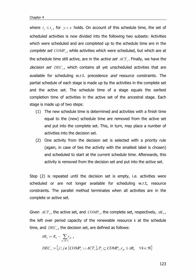
Chapter 4
123
where xy tt , for xy holds. On account of this schedule time, the set of
scheduled activities is now divided into the following two subsets: Activities
which were scheduled and are completed up to the schedule time are in the
complete set xCOMP , while activities which were scheduled, but which are at
the schedule time still active, are in the active set xACT . Finally, we have the
decision set xDEC , which contains all yet unscheduled activities that are
available for scheduling w.r.t. precedence and resource constraints. The
partial schedule of each stage is made up by the activities in the complete set
and the active set. The schedule time of a stage equals the earliest
completion time of activities in the active set of the ancestral stage. Each
stage is made up of two steps:
(1) The new schedule time is determined and activities with a finish time
equal to the (new) schedule time are removed from the active set
and put into the complete set. This, in turn, may place a number of
activities into the decision set.
(2) One activity from the decision set is selected with a priority rule
(again, in case of ties the activity with the smallest label is chosen)
and scheduled to start at the current schedule time. Afterwards, this
activity is removed from the decision set and put into the active set.
Step (2) is repeated until the decision set is empty, i.e. activities were
scheduled or are not longer available for scheduling w.r.t, resource
constraints. The parallel method terminates when all activities are in the
complete or active set.
Given xACT , the active set, and xCOMP , the complete set, respectively, kK ,
the left over period capacity of the renewable resource k at the schedule
time, and xDEC , the decision set, are defined as follows:
xACTj
jkkk rRR : ,
kRrCOMPPACTCOMPjjDEC kjkxjxxx ,,|:
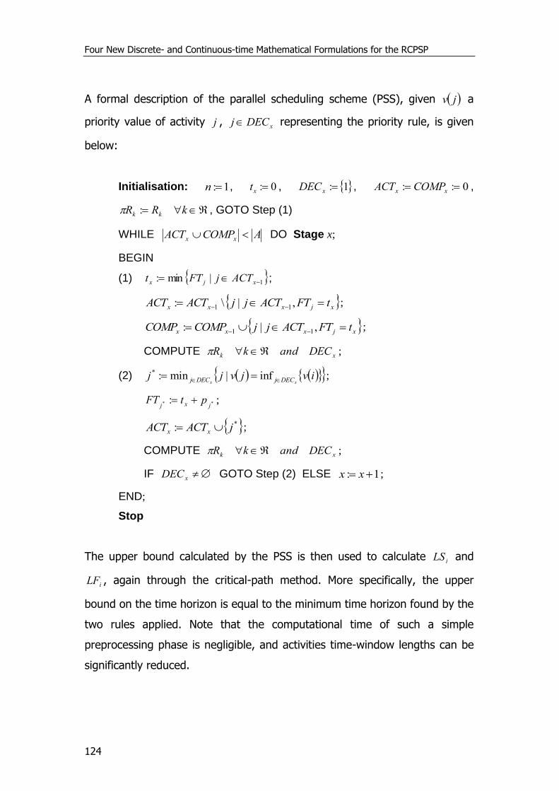
Four New Discrete- and Continuous-time Mathematical Formulations for the RCPSP
124
A formal description of the parallel scheduling scheme (PSS), given jv a
priority value of activity j , xDECj representing the priority rule, is given
below:
Initialisation: 1:n , 0:xt , 1:xDEC , 0:: xx COMPACT ,
kRR kk : , GOTO Step (1)
WHILE ACOMPACT xx DO Stage x;
BEGIN
(1) 1|min: xjx ACTjFTt ;
xjxxx tFTACTjjACTACT ,|\: 11
;
xjxxx tFTACTjjCOMPCOMP ,|: 11
;
COMPUTE xk DECandkR ;
(2) ivjvjjxx DECjDECj inf|min:* ;
** : jxjptFT ;
*: jACTACT xx ;
COMPUTE xk DECandkR ;
IF xDEC GOTO Step (2) ELSE 1: xx ;
END;
Stop
The upper bound calculated by the PSS is then used to calculate iLS and
iLF , again through the critical-path method. More specifically, the upper
bound on the time horizon is equal to the minimum time horizon found by the
two rules applied. Note that the computational time of such a simple
preprocessing phase is negligible, and activities time-window lengths can be
significantly reduced.
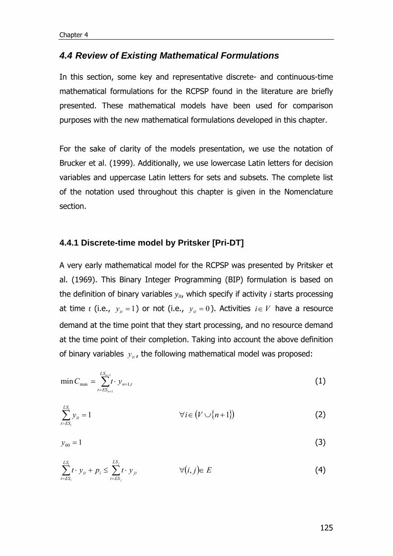
Chapter 4
125
4.4 Review of Existing Mathematical Formulations
In this section, some key and representative discrete- and continuous-time
mathematical formulations for the RCPSP found in the literature are briefly
presented. These mathematical models have been used for comparison
purposes with the new mathematical formulations developed in this chapter.
For the sake of clarity of the models presentation, we use the notation of
Brucker et al. (1999). Additionally, we use lowercase Latin letters for decision
variables and uppercase Latin letters for sets and subsets. The complete list
of the notation used throughout this chapter is given in the Nomenclature
section.
4.4.1 Discrete-time model by Pritsker [Pri-DT]
A very early mathematical model for the RCPSP was presented by Pritsker et
al. (1969). This Binary Integer Programming (BIP) formulation is based on
the definition of binary variables yit, which specify if activity i starts processing
at time t (i.e., 1ity ) or not (i.e., 0ity ). Activities Vi have a resource
demand at the time point that they start processing, and no resource demand
at the time point of their completion. Taking into account the above definition
of binary variables ity , the following mathematical model was proposed:
1
1
,1maxminn
n
LS
ESt
tnytC (1)
1
i
i
LS
ESt
ity 1 nVi (2)
100 y (3)
j
j
i
i
LS
ESt
jti
LS
ESt
it ytpyt Eji , (4)
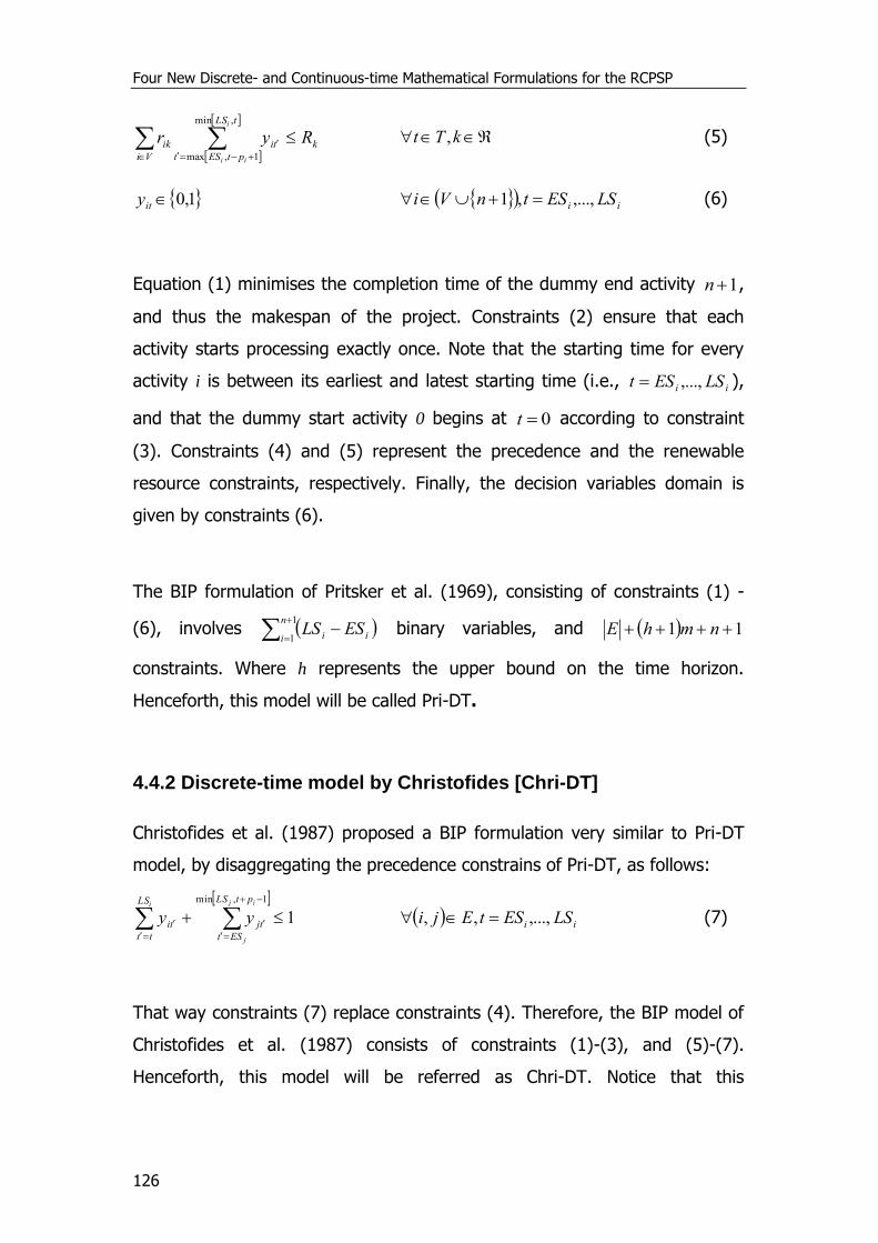
Four New Discrete- and Continuous-time Mathematical Formulations for the RCPSP
126
k
Vi
ti
tLS
ptESt
ik Ryri
ii
,min
1,max
kTt , (5)
1,0ity ii LSEStnVi ,...,,1 (6)
Equation (1) minimises the completion time of the dummy end activity 1n ,
and thus the makespan of the project. Constraints (2) ensure that each
activity starts processing exactly once. Note that the starting time for every
activity i is between its earliest and latest starting time (i.e., ii LSESt ,..., ),
and that the dummy start activity 0 begins at 0t according to constraint
(3). Constraints (4) and (5) represent the precedence and the renewable
resource constraints, respectively. Finally, the decision variables domain is
given by constraints (6).
The BIP formulation of Pritsker et al. (1969), consisting of constraints (1) -
(6), involves
1
1
n
i ii ESLS binary variables, and 11 nmhE
constraints. Where h represents the upper bound on the time horizon.
Henceforth, this model will be called Pri-DT.
4.4.2 Discrete-time model by Christofides [Chri-DT]
Christofides et al. (1987) proposed a BIP formulation very similar to Pri-DT
model, by disaggregating the precedence constrains of Pri-DT, as follows:
1
1,min
ij
j
iptLS
ESt
tj
LS
tt
ti yy ii LSEStEji ,...,,, (7)
That way constraints (7) replace constraints (4). Therefore, the BIP model of
Christofides et al. (1987) consists of constraints (1)-(3), and (5)-(7).
Henceforth, this model will be referred as Chri-DT. Notice that this
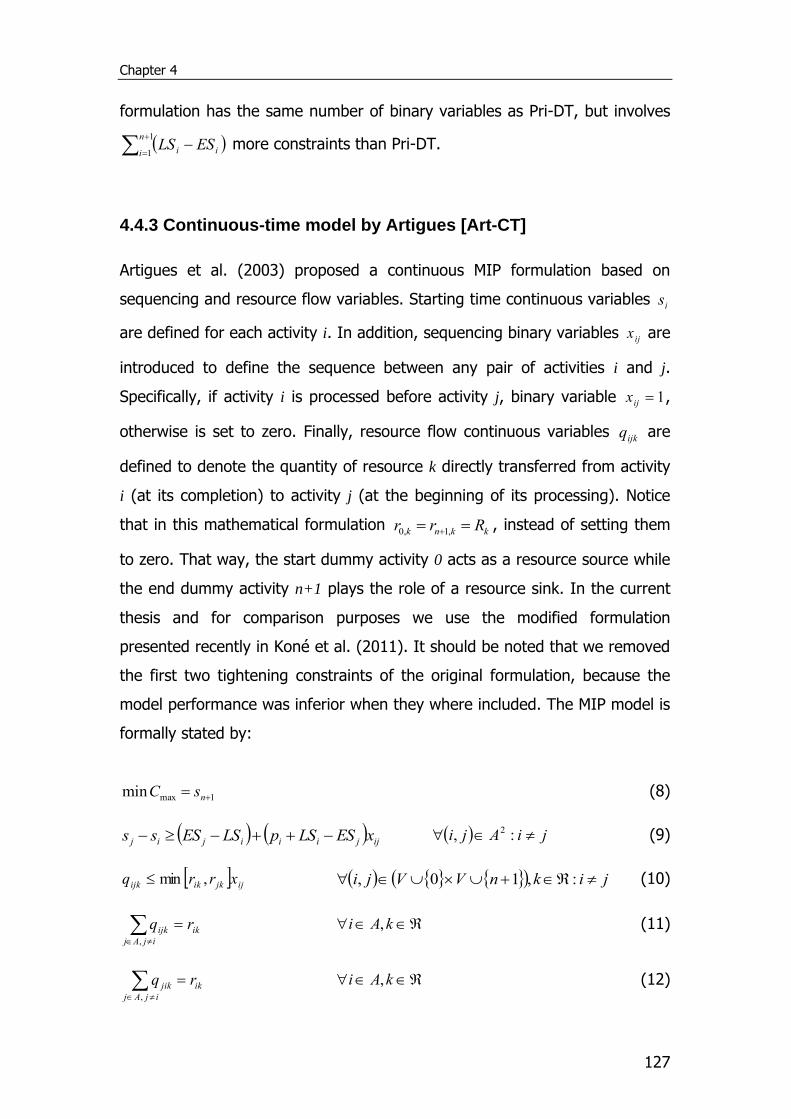
Chapter 4
127
formulation has the same number of binary variables as Pri-DT, but involves
1
1
n
i ii ESLS more constraints than Pri-DT.
4.4.3 Continuous-time model by Artigues [Art-CT]
Artigues et al. (2003) proposed a continuous MIP formulation based on
sequencing and resource flow variables. Starting time continuous variables is
are defined for each activity i. In addition, sequencing binary variables ijx are
introduced to define the sequence between any pair of activities i and j.
Specifically, if activity i is processed before activity j, binary variable 1ijx ,
otherwise is set to zero. Finally, resource flow continuous variables ijkq are
defined to denote the quantity of resource k directly transferred from activity
i (at its completion) to activity j (at the beginning of its processing). Notice
that in this mathematical formulation kknk Rrr ,1,0, instead of setting them
to zero. That way, the start dummy activity 0 acts as a resource source while
the end dummy activity n+1 plays the role of a resource sink. In the current
thesis and for comparison purposes we use the modified formulation
presented recently in Koné et al. (2011). It should be noted that we removed
the first two tightening constraints of the original formulation, because the
model performance was inferior when they where included. The MIP model is
formally stated by:
1maxmin nsC (8)
ijjiiijij xESLSpLSESss jiAji :, 2 (9)
ijjkikijk xrrq ,min jiknVVji :,10, (10)
ik
ijAj
ijk rq ,
kAi , (11)
ik
ijAj
jik rq ,
kAi , (12)
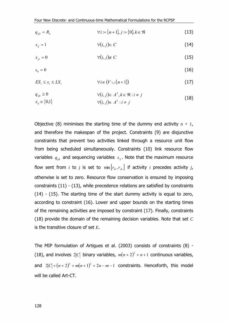
Four New Discrete- and Continuous-time Mathematical Formulations for the RCPSP
128
kijk Rq kjni ,0:,1: (13)
1ijx Cji , (14)
0jix Cji , (15)
00 s (16)
iii LSsES 1 nVi (17)
1,0
0
ij
ijk
x
q
jiAji
jikAji
:,
:,,
2
2
(18)
Objective (8) minimises the starting time of the dummy end activity n + 1,
and therefore the makespan of the project. Constraints (9) are disjunctive
constraints that prevent two activities linked through a resource unit flow
from being scheduled simultaneously. Constraints (10) link resource flow
variables ijkq and sequencing variables ijx . Note that the maximum resource
flow sent from i to j is set to jkik rr ,min if activity i precedes activity j,
otherwise is set to zero. Resource flow conservation is ensured by imposing
constraints (11) - (13), while precedence relations are satisfied by constraints
(14) - (15). The starting time of the start dummy activity is equal to zero,
according to constraint (16). Lower and upper bounds on the starting times
of the remaining activities are imposed by constraint (17). Finally, constraints
(18) provide the domain of the remaining decision variables. Note that set C
is the transitive closure of set E.
The MIP formulation of Artigues et al. (2003) consists of constraints (8) -
(18), and involves C2 binary variables, 122
nnm continuous variables,
and 1212222
mnnmnC constraints. Henceforth, this model
will be called Art-CT.
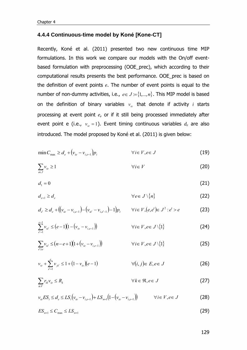
Chapter 4
129
4.4.4 Continuous-time model by Koné [Kone-CT]
Recently, Koné et al. (2011) presented two new continuous time MIP
formulations. In this work we compare our models with the On/off event-
based formulation with preprocessing (OOE_prec), which according to their
computational results presents the best performance. OOE_prec is based on
the definition of event points e. The number of event points is equal to the
number of non-dummy activities, i.e., nJe ,...,1: . This MIP model is based
on the definition of binary variables iev that denote if activity i starts
processing at event point e, or if it still being processed immediately after
event point e (i.e., 1iev ). Event timing continuous variables de are also
introduced. The model proposed by Koné et al. (2011) is given below:
ieiiee pvvdC 1,maxmin JeVi , (19)
1Je
iev Vi (20)
01 d (21)
ee dd 1 nJe \ (22)
ieieieiieee pvvvvdd 11,1, eeJeeVi :,, 2 (23)
1,
1
1
11
eiie
e
e
ei vvev 1\, JeVi (24)
1,11
eiie
ee
ei vvenv 1\, JeVi (25)
1111
evvv ie
e
e
ejie JeEji ,, (26)
k
Vi
ieik Rvr
Jek , (27)
1,11, 1 eiieneiieieiie vvLSvvLSdESv JeVi , (28)
1max1 nn LSCES (29)
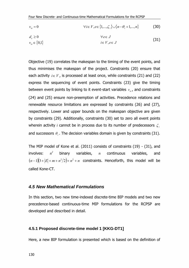
Four New Discrete- and Continuous-time Mathematical Formulations for the RCPSP
130
0iev nneVi ii ,...,1,...,1, (30)
1,0
0
ie
e
v
d
JeVi
Je
, (31)
Objective (19) correlates the makespan to the timing of the event points, and
thus minimises the makespan of the project. Constraints (20) ensure that
each activity Vi , is processed at least once, while constraints (21) and (22)
express the sequencing of event points. Constraints (23) give the timing
between event points by linking to it event-start variables iev , and constraints
(24) and (25) ensure non-preemption of activities. Precedence relations and
renewable resource limitations are expressed by constraints (26) and (27),
respectively. Lower and upper bounds on the makespan objective are given
by constraints (29). Additionally, constraints (30) set to zero all event points
wherein activity i cannot be in process due to its number of predecessors i
and successors i . The decision variables domain is given by constraints (31).
The MIP model of Kone et al. (2011) consists of constraints (19) - (31), and
involves: n2 binary variables, n continuous variables, and
nnnmEn 22 231 constraints. Henceforth, this model will be
called Kone-CT.
4.5 New Mathematical Formulations
In this section, two new time-indexed discrete-time BIP models and two new
precedence-based continuous-time MIP formulations for the RCPSP are
developed and described in detail.
4.5.1 Proposed discrete-time model 1 [KKG-DT1]
Here, a new BIP formulation is presented which is based on the definition of
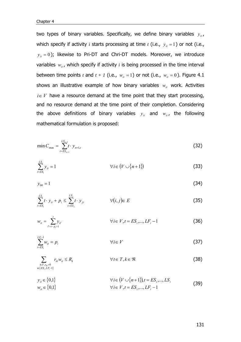
Chapter 4
131
two types of binary variables. Specifically, we define binary variables ity ,
which specify if activity i starts processing at time t (i.e., 1ity ) or not (i.e.,
0ity ); likewise to Pri-DT and Chri-DT models. Moreover, we introduce
variables itw , which specify if activity i is being processed in the time interval
between time points t and t + 1 (i.e., 1itw ) or not (i.e., 0itw ). Figure 4.1
shows an illustrative example of how binary variables itw work. Activities
Vi have a resource demand at the time point that they start processing,
and no resource demand at the time point of their completion. Considering
the above definitions of binary variables ity and itw , the following
mathematical formulation is proposed:
1
1
,1maxminn
n
LS
ESt
tnytC (32)
1
i
i
LS
ESt
ity 1 nVi (33)
100 y (34)
j
j
i
i
LS
ESt
jti
LS
ESt
it ytpyt Eji , (35)
t
ptt
tiit
i
yw1
1,...,, ii LFEStVi (36)
i
LF
ESt
it pwi
i
1
Vi (37)
kitik
LFESt
rVi
Rwr
ii
ik
1,
0,
kTt , (38)
1,0
1,0
it
it
w
y
1,...,,
,...,,1
ii
ii
LFEStVi
LSEStnVi (39)
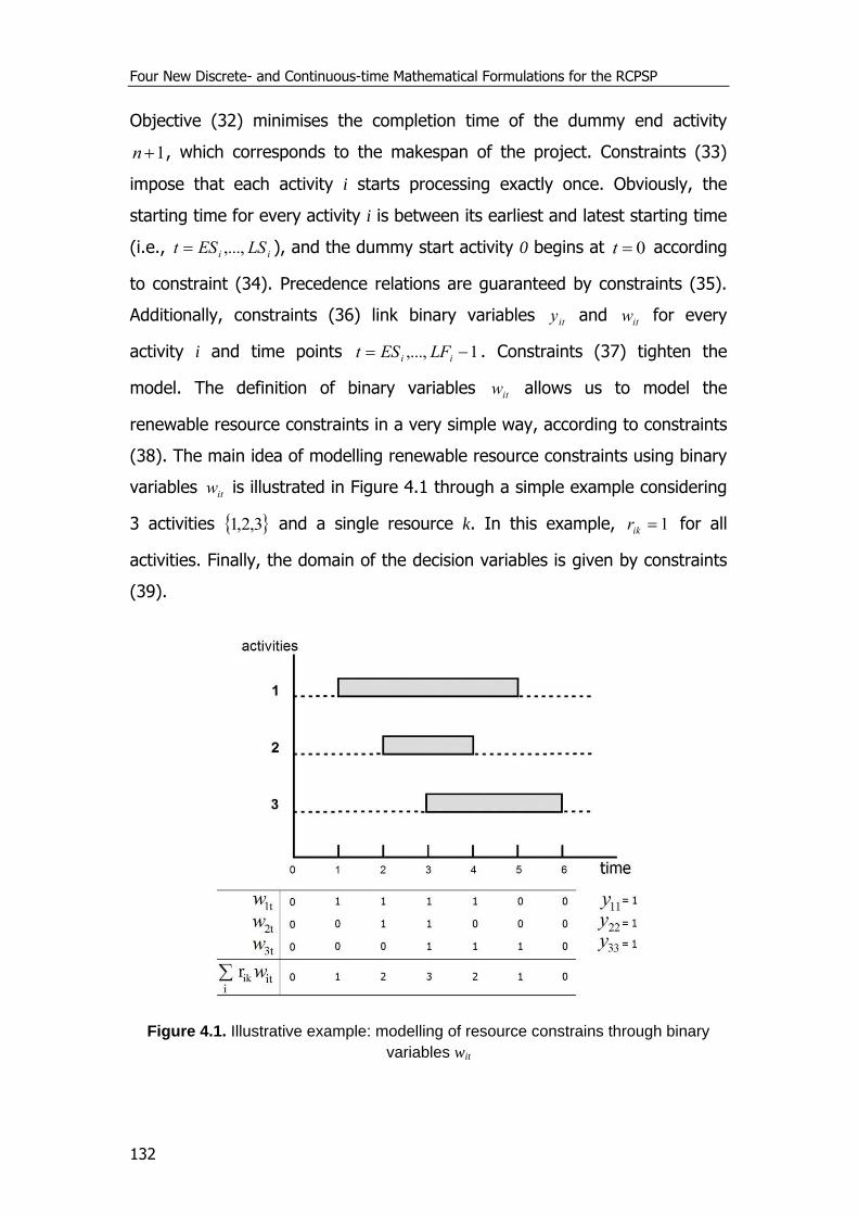
Four New Discrete- and Continuous-time Mathematical Formulations for the RCPSP
132
Objective (32) minimises the completion time of the dummy end activity
1n , which corresponds to the makespan of the project. Constraints (33)
impose that each activity i starts processing exactly once. Obviously, the
starting time for every activity i is between its earliest and latest starting time
(i.e., ii LSESt ,..., ), and the dummy start activity 0 begins at 0t according
to constraint (34). Precedence relations are guaranteed by constraints (35).
Additionally, constraints (36) link binary variables ity and itw for every
activity i and time points 1,..., ii LFESt . Constraints (37) tighten the
model. The definition of binary variables itw allows us to model the
renewable resource constraints in a very simple way, according to constraints
(38). The main idea of modelling renewable resource constraints using binary
variables itw is illustrated in Figure 4.1 through a simple example considering
3 activities 3,2,1 and a single resource k. In this example, 1ikr for all
activities. Finally, the domain of the decision variables is given by constraints
(39).
Figure 4.1. Illustrative example: modelling of resource constrains through binary
variables wit
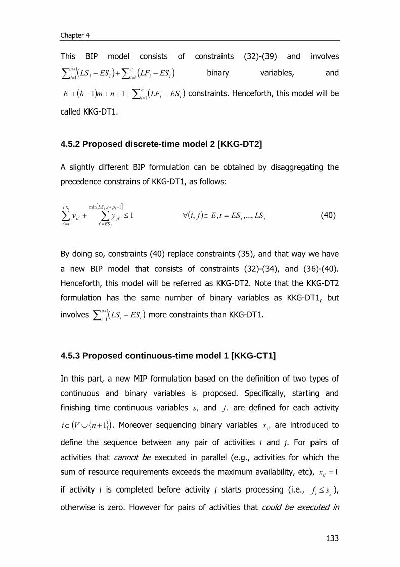
Chapter 4
133
This BIP model consists of constraints (32)-(39) and involves
n
i ii
n
i ii ESLFESLS1
1
1 binary variables, and
n
i ii ESLFnmhE1
11 constraints. Henceforth, this model will be
called KKG-DT1.
4.5.2 Proposed discrete-time model 2 [KKG-DT2]
A slightly different BIP formulation can be obtained by disaggregating the
precedence constrains of KKG-DT1, as follows:
1
1,min
ij
j
iptLS
ESt
tj
LS
tt
ti yy ii LSEStEji ,...,,, (40)
By doing so, constraints (40) replace constraints (35), and that way we have
a new BIP model that consists of constraints (32)-(34), and (36)-(40).
Henceforth, this model will be referred as KKG-DT2. Note that the KKG-DT2
formulation has the same number of binary variables as KKG-DT1, but
involves
1
1
n
i ii ESLS more constraints than KKG-DT1.
4.5.3 Proposed continuous-time model 1 [KKG-CT1]
In this part, a new MIP formulation based on the definition of two types of
continuous and binary variables is proposed. Specifically, starting and
finishing time continuous variables is and if are defined for each activity
1 nVi . Moreover sequencing binary variables ijx are introduced to
define the sequence between any pair of activities i and j. For pairs of
activities that cannot be executed in parallel (e.g., activities for which the
sum of resource requirements exceeds the maximum availability, etc), 1ijx
if activity i is completed before activity j starts processing (i.e., ji sf ),
otherwise is zero. However for pairs of activities that could be executed in
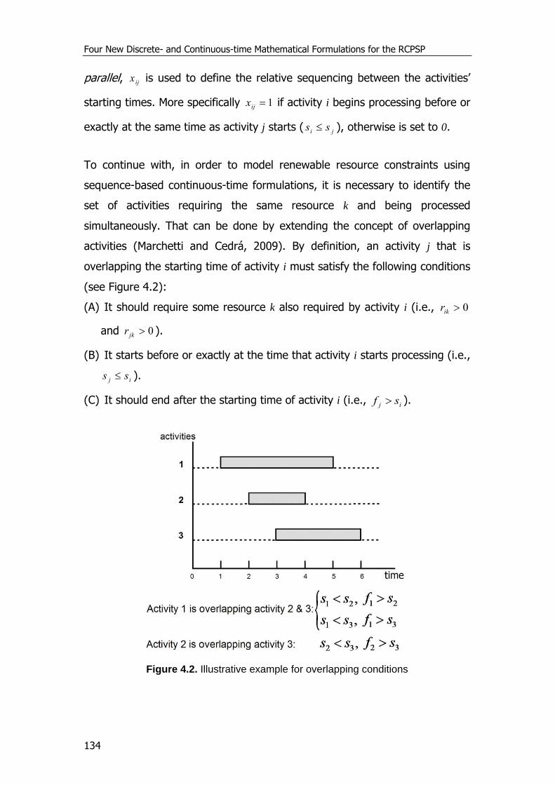
Four New Discrete- and Continuous-time Mathematical Formulations for the RCPSP
134
parallel, ijx is used to define the relative sequencing between the activities’
starting times. More specifically 1ijx if activity i begins processing before or
exactly at the same time as activity j starts ( ji ss ), otherwise is set to 0.
To continue with, in order to model renewable resource constraints using
sequence-based continuous-time formulations, it is necessary to identify the
set of activities requiring the same resource k and being processed
simultaneously. That can be done by extending the concept of overlapping
activities (Marchetti and Cedrá, 2009). By definition, an activity j that is
overlapping the starting time of activity i must satisfy the following conditions
(see Figure 4.2):
(A) It should require some resource k also required by activity i (i.e., 0ikr
and 0jkr ).
(B) It starts before or exactly at the time that activity i starts processing (i.e.,
ij ss ).
(C) It should end after the starting time of activity i (i.e., ij sf ).
Figure 4.2. Illustrative example for overlapping conditions
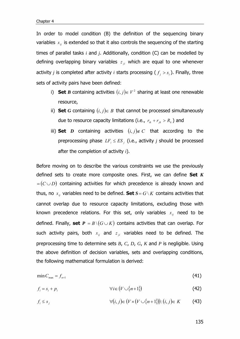
Chapter 4
135
In order to model condition (B) the definition of the sequencing binary
variables ijx is extended so that it also controls the sequencing of the starting
times of parallel tasks i and j. Additionally, condition (C) can be modelled by
defining overlapping binary variables jiz which are equal to one whenever
activity j is completed after activity i starts processing (ij sf ). Finally, three
sets of activity pairs have been defined:
i) Set B containing activities 2, Vji sharing at least one renewable
resource,
ii) Set G containing Bji , that cannot be processed simultaneously
due to resource capacity limitations (i.e., kjkik Rrr ) and
iii) Set D containing activities Cji , that according to the
preprocessing phase ji ESLF (i.e., activity j should be processed
after the completion of activity i).
Before moving on to describe the various constraints we use the previously
defined sets to create more composite ones. First, we can define Set K
DC containing activities for which precedence is already known and
thus, no ijx variables need to be defined. Set S KG \ contains activities that
cannot overlap due to resource capacity limitations, excluding those with
known precedence relations. For this set, only variables ijx need to be
defined. Finally, set P KGB \ contains activities that can overlap. For
such activity pairs, both ijx and jiz variables need to be defined. The
preprocessing time to determine sets B, C, D, G, K and P is negligible. Using
the above definition of decision variables, sets and overlapping conditions,
the following mathematical formulation is derived:
1maxmin nfC (41)
iii psf 1 nVi (42)
ji sf KjinVVji ,:1, (43)
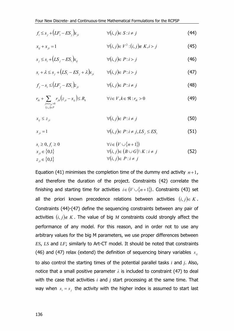
Four New Discrete- and Continuous-time Mathematical Formulations for the RCPSP
136
jijiji xESLFsf jiSji :, (44)
1 jiij xx jiKjiVji ,,:, 2 (45)
ijijij xESLSss jiPji :, (46)
jijiji xESLSss jiPji :, (47)
jiijij zESLFsf jiPji :, (48)
kijjijk
Pji
rij
ik Rxzrrjk
,
0:
0:, ikrkVi (49)
jiij zx jiPji :, (50)
1jix ij ESLSjiPji ,:, (51)
1,0
1,0
0,0
ji
ji
ii
z
x
fs
jiPji
jiKGBji
nVi
:,
:\,
1
(52)
Equation (41) minimises the completion time of the dummy end activity 1n ,
and therefore the duration of the project. Constraints (42) correlate the
finishing and starting time for activities 1 nVi . Constraints (43) set
all the priori known precedence relations between activities Kji , .
Constraints (44)-(47) define the sequencing constraints between any pair of
activities Kji , . The value of big M constraints could strongly affect the
performance of any model. For this reason, and in order not to use any
arbitrary values for the big M parameters, we use proper differences between
ES, LS and LF; similarly to Art-CT model. It should be noted that constraints
(46) and (47) relax (extend) the definition of sequencing binary variables ijx
to also control the starting times of the potential parallel tasks i and j. Also,
notice that a small positive parameter λ is included to constraint (47) to deal
with the case that activities i and j start processing at the same time. That
way when ji ss the activity with the higher index is assumed to start last

Chapter 4
137
(i.e., if ji ss and ji , then 1jix ). In the case studies we used a value of
0.1 for parameter λ. Overlapping condition (C) is modelled by constraints
(48), while renewable resource constraints are given by constraints (49). By
using ijji xz we are able to detect activity overlapping and properly model
the resource constraints.
Constraints (46) – (49) state that if activity i starts processing before activity j
(i.e., 1ijx ), then activity j has to finish after activity i starts (i.e., 1jiz ).
The only case that the difference ijji xz takes the value of 1 is when
activity j overlaps i. That means, according to the definition of overlapping
given above, that j finishes after i starts (i.e., 1jiz ) and activity j starts
processing before i (i.e., 0ijx ). Constraints (50) are tightening constraints
that correlate directly sequencing and overlapping binary variables. It can be
easily proven that for activities which could overlap Pji , , if 1ijx that
means that jji fss , and consequently 0 ij sf which according to
constraints (48) gives 1jiz .
Table 4.1 displays all possible combinations for variables jiz and ijx for
activities Pji , that could be executed in parallel. In the first two cases
wherein 0jiz , no overlapping occurs since activity i starts after the
completion of activity j (i.e., ijj sfs ). Especially, in the second case,
notice that if 0jiz and 1ijx that would mean that jij ssf , which
obviously is impossible. For this reason, if 0jiz then always 0ijx . In the
last two cases wherein 1jiz , overlapping occurs if and only if activity j
begins processing before activity i starts (i.e., 0ijx ), because in that case
holds jij fss . Further, the sequencing binary variables for activities
Pji , that ij ESLS can be fixed due to the preprocessing phase,
according to constraints (51). Finally, the domain of the decision variables is
given by constraints (52).
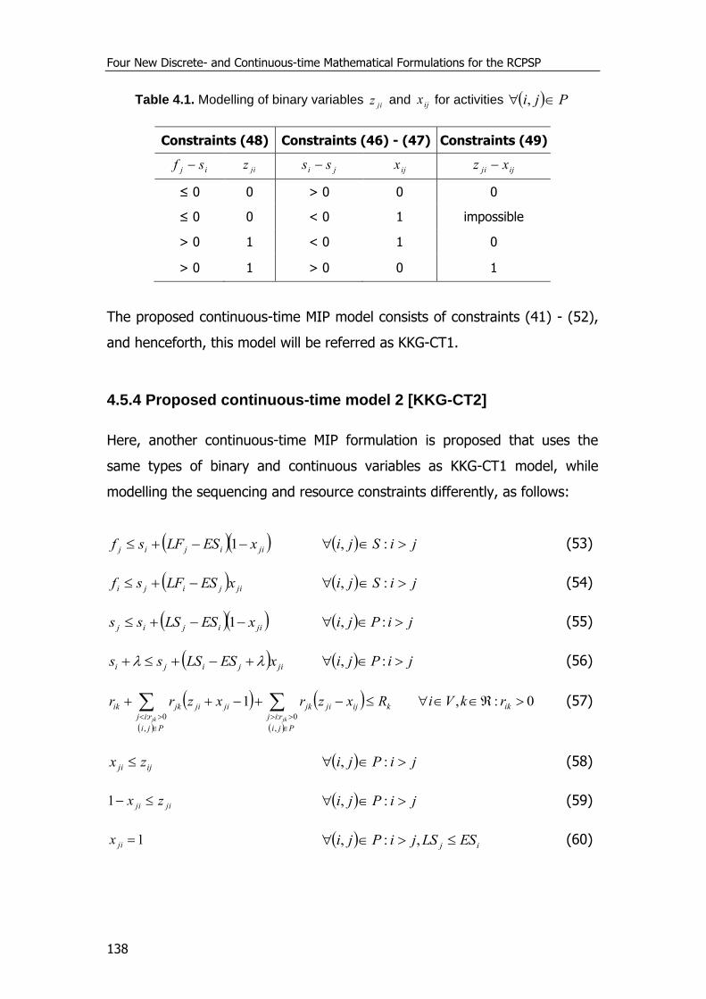
Four New Discrete- and Continuous-time Mathematical Formulations for the RCPSP
138
Table 4.1. Modelling of binary variables jiz and ijx for activities Pji ,
Constraints (48) Constraints (46) - (47) Constraints (49)
ij sf jiz ji ss ijx ijji xz
≤ 0 0 > 0 0 0
≤ 0 0 < 0 1 impossible
> 0 1 < 0 1 0
> 0 1 > 0 0 1
The proposed continuous-time MIP model consists of constraints (41) - (52),
and henceforth, this model will be referred as KKG-CT1.
4.5.4 Proposed continuous-time model 2 [KKG-CT2]
Here, another continuous-time MIP formulation is proposed that uses the
same types of binary and continuous variables as KKG-CT1 model, while
modelling the sequencing and resource constraints differently, as follows:
jiijij xESLFsf 1 jiSji :, (53)
jijiji xESLFsf jiSji :, (54)
jiijij xESLSss 1 jiPji :, (55)
jijiji xESLSss jiPji :, (56)
kijjijk
Pji
rij
jijijk
Pji
rij
ik Rxzrxzrrjkjk
,
0:
,
0:
1 0:, ikrkVi (57)
ijji zx jiPji :, (58)
jiji zx 1 jiPji :, (59)
1jix ij ESLSjiPji ,:, (60)
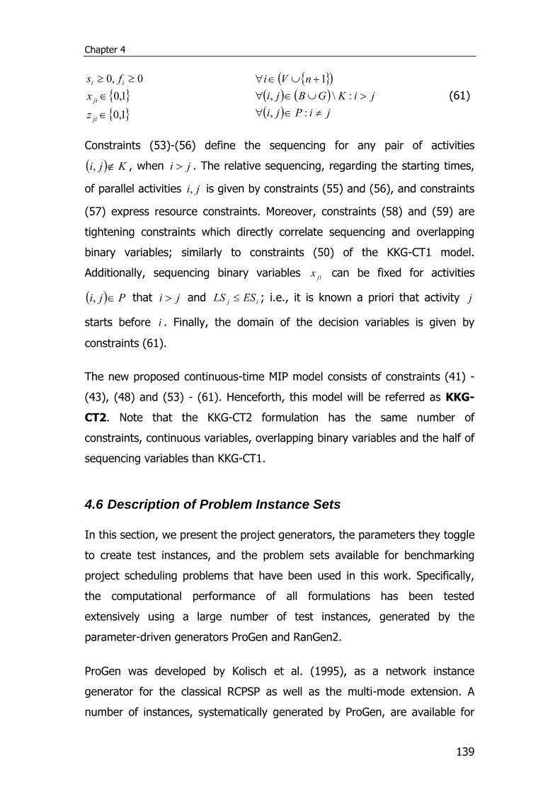
Chapter 4
139
1,0
1,0
0,0
ji
ji
ii
z
x
fs
jiPji
jiKGBji
nVi
:,
:\,
1
(61)
Constraints (53)-(56) define the sequencing for any pair of activities
Kji , , when ji . The relative sequencing, regarding the starting times,
of parallel activities ji, is given by constraints (55) and (56), and constraints
(57) express resource constraints. Moreover, constraints (58) and (59) are
tightening constraints which directly correlate sequencing and overlapping
binary variables; similarly to constraints (50) of the KKG-CT1 model.
Additionally, sequencing binary variables jix can be fixed for activities
Pji , that ji and ij ESLS ; i.e., it is known a priori that activity j
starts before i . Finally, the domain of the decision variables is given by
constraints (61).
The new proposed continuous-time MIP model consists of constraints (41) -
(43), (48) and (53) - (61). Henceforth, this model will be referred as KKG-
CT2. Note that the KKG-CT2 formulation has the same number of
constraints, continuous variables, overlapping binary variables and the half of
sequencing variables than KKG-CT1.
4.6 Description of Problem Instance Sets
In this section, we present the project generators, the parameters they toggle
to create test instances, and the problem sets available for benchmarking
project scheduling problems that have been used in this work. Specifically,
the computational performance of all formulations has been tested
extensively using a large number of test instances, generated by the
parameter-driven generators ProGen and RanGen2.
ProGen was developed by Kolisch et al. (1995), as a network instance
generator for the classical RCPSP as well as the multi-mode extension. A
number of instances, systematically generated by ProGen, are available for
Four New Discrete- and Continuous-time Mathematical Formulations for the RCPSP
140
researchers in PSPLIB (Kolisch and Sprecher, 1996), an online scheduling
library (http://129.187.106.231/psplib/). PSPLIB test sets have been used as
a benchmark in a large number of studies. These instances were generated
by varying the Network Complexity (NC), Resource Factor (RF) and Resource
Strength (RS) parameter values. NC is the average number of non-redundant
arcs per activity (node), including the dummy source and sink activities. RF
reflects the average quantity of resources required per activity, and is
normalised in the interval [0,1]. A value of 1 suggests that all activities
require all resources, while a value of 0, that no resource is required by any
activity (which corresponds to the unconstrained case). The RS parameter
measures the strength of the resource constraints. It is a scaling parameter
expressing resource availability as a convex combination of a minimum and
maximum level with values in the interval [0,1]. In this work, we use the
problem sets with 30 and 60 activities, utilizing 4 renewable resources. Each
problem set comprises of 480 test problem instances. In the PSPLIB problem
instances the parameters values are:
NC = {1.50, 1.80, 2.10},
RF = {0.25, 0.50, 0.75, 1.00}
RS = {0.20, 0.50, 0.70, 1.00}
Henceforth, the 480 problem instance test sets with 30 and 60 activities will
be referred to as j30 and j60, respectively.
Vanhoucke et al. (2008) developed RanGen2 which is a random project
network generator for single- and multi-mode project instances, extending
RanGen (Demeulemeester et al., 2003) by incorporating further topological
network measures. RanGen and RanGen2 use different measures than
ProGen. These six topological measures are displayed in Table 4.2. The first
five indicators (I1 to I5) are based on the indicators proposed by Tavares et al.
(1999). More specifically, I1, I2 and I4 are exact copies of the original ones,
while I3 and I5 are improved versions. The last indicator I6 is totally new. In
our computational comparison we used the 1800 problem instances
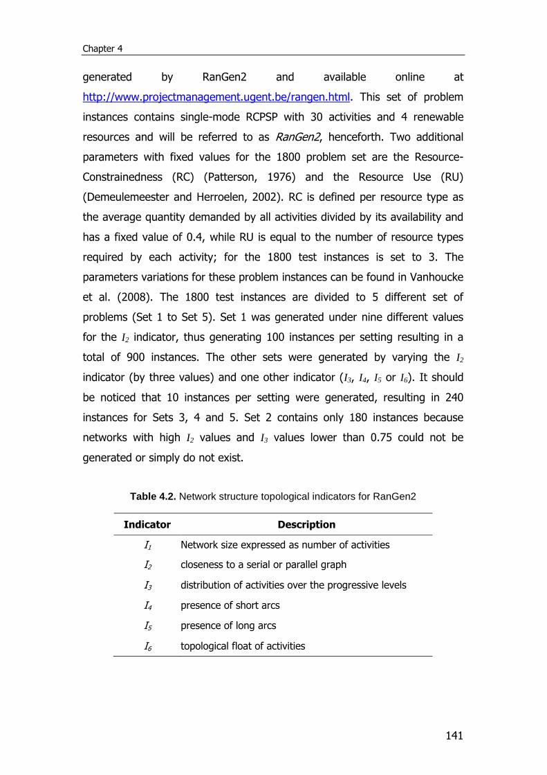
Chapter 4
141
generated by RanGen2 and available online at
http://www.projectmanagement.ugent.be/rangen.html. This set of problem
instances contains single-mode RCPSP with 30 activities and 4 renewable
resources and will be referred to as RanGen2, henceforth. Two additional
parameters with fixed values for the 1800 problem set are the Resource-
Constrainedness (RC) (Patterson, 1976) and the Resource Use (RU)
(Demeulemeester and Herroelen, 2002). RC is defined per resource type as
the average quantity demanded by all activities divided by its availability and
has a fixed value of 0.4, while RU is equal to the number of resource types
required by each activity; for the 1800 test instances is set to 3. The
parameters variations for these problem instances can be found in Vanhoucke
et al. (2008). The 1800 test instances are divided to 5 different set of
problems (Set 1 to Set 5). Set 1 was generated under nine different values
for the I2 indicator, thus generating 100 instances per setting resulting in a
total of 900 instances. The other sets were generated by varying the I2
indicator (by three values) and one other indicator (I3, I4, I5 or I6). It should
be noticed that 10 instances per setting were generated, resulting in 240
instances for Sets 3, 4 and 5. Set 2 contains only 180 instances because
networks with high I2 values and I3 values lower than 0.75 could not be
generated or simply do not exist.
Table 4.2. Network structure topological indicators for RanGen2
Indicator Description
I1 Network size expressed as number of activities
I2 closeness to a serial or parallel graph
I3 distribution of activities over the progressive levels
I4 presence of short arcs
I5 presence of long arcs
I6 topological float of activities
Four New Discrete- and Continuous-time Mathematical Formulations for the RCPSP
142
4.7 Computational Comparison Study
This section summarises the computational comparison between some
existing representative formulations and the four new mathematical
formulations presented in Sections 4.4 and 4.5, respectively. Here, we
present the computational results for all formulations, and further analyse
and discuss the computational performance of the models considered. Notice
that our experimental computational study involves a total number of 2760
RCPSP problems, considering the 3 benchmark RCPSP problem sets j30, j60
and RanGen2 described in the previous section. All mathematical formulations
have been solved on an Intel Core i5 CPU M430 2.27GHz with 4GB RAM using
CPLEX 11.1.1 via a GAMS 22.8.1 (Rosenthal, 2012) WIN 6007.6015 VIS
interface under standard configurations. A maximum resource time limit of
600 CPU s has been set for all problem instances.
A description of the notation used in the computational results follows.
Feasible (%) is the percentage of instances that gave an integer solution
(i.e., optimal, suboptimal, or not-proven optimal) within the predefined time
limit. Good (%) is the percentage of instances that gave a good integer
solution (i.e., optimal, or suboptimal with a gap lower than 3% from the
optimal solution) within the predefined time limit. Optimal (%) represents the
percentage of (proven) optimal solutions found within the time limit. Gap (%)
is the average gap of the integer non-proven optimal solutions from the real
optimal solution, or the best known solution if optimal solution is not available
(some problems in j60 and RanGen2). ΔHEUR (%) stands for the average
deviation of the optimal solution from the upper bound calculated by the
preprocessing stage, taking into account only instances that were solved to
optimality. Similarly, ΔCPM (%) is the average deviation of the optimal
solution found from the lower bound calculated through the critical-path
method. Finally, Optimal CPU (s) is the average CPU time required for
instances solved to optimality.
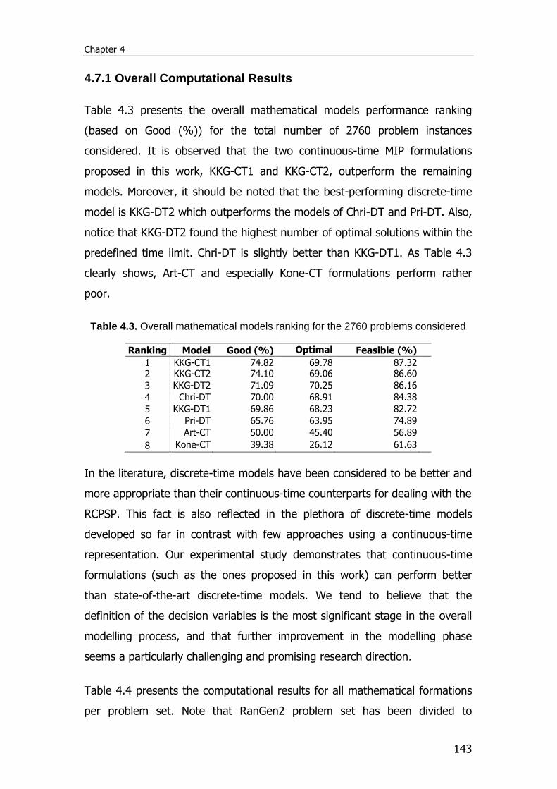
Chapter 4
143
4.7.1 Overall Computational Results
Table 4.3 presents the overall mathematical models performance ranking
(based on Good (%)) for the total number of 2760 problem instances
considered. It is observed that the two continuous-time MIP formulations
proposed in this work, KKG-CT1 and KKG-CT2, outperform the remaining
models. Moreover, it should be noted that the best-performing discrete-time
model is KKG-DT2 which outperforms the models of Chri-DT and Pri-DT. Also,
notice that KKG-DT2 found the highest number of optimal solutions within the
predefined time limit. Chri-DT is slightly better than KKG-DT1. As Table 4.3
clearly shows, Art-CT and especially Kone-CT formulations perform rather
poor.
Table 4.3. Overall mathematical models ranking for the 2760 problems considered
Ranking Model Good (%) Optimal (%)
Feasible (%)
1 KKG-CT1 74.82 69.78 87.32 2 KKG-CT2 74.10 69.06 86.60
3 KKG-DT2 71.09 70.25 86.16
4 Chri-DT 70.00 68.91 84.38
5 KKG-DT1 69.86 68.23 82.72
6 Pri-DT 65.76 63.95 74.89
7 Art-CT 50.00 45.40 56.89
8 Kone-CT 39.38 26.12 61.63
In the literature, discrete-time models have been considered to be better and
more appropriate than their continuous-time counterparts for dealing with the
RCPSP. This fact is also reflected in the plethora of discrete-time models
developed so far in contrast with few approaches using a continuous-time
representation. Our experimental study demonstrates that continuous-time
formulations (such as the ones proposed in this work) can perform better
than state-of-the-art discrete-time models. We tend to believe that the
definition of the decision variables is the most significant stage in the overall
modelling process, and that further improvement in the modelling phase
seems a particularly challenging and promising research direction.
Table 4.4 presents the computational results for all mathematical formations
per problem set. Note that RanGen2 problem set has been divided to
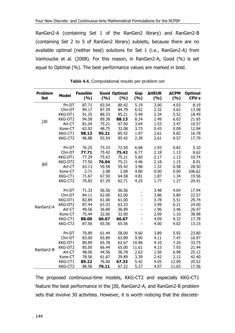
Four New Discrete- and Continuous-time Mathematical Formulations for the RCPSP
144
RanGen2-A (containing Set 1 of the RanGen2 library) and RanGen2-B
(containing Set 2 to 5 of RanGen2 library) subsets, because there are no
available optimal (neither best) solutions for Set 1 (i.e., RanGen2-A) from
Vanhoucke et al. (2008). For this reason, in RanGen2-A, Good (%) is set
equal to Optimal (%). The best performance values are marked in bold.
Table 4.4. Computational results per problem set
Problem Set
Model Feasible
(%) Good (%)
Optimal (%)
Gap (%)
ΔHEUR (%)
ΔCPM (%)
Optimal CPU s
j30
Pri-DT 87.71 83.54 80.42 5.19 2.00 4.03 8.19 Chri-DT 94.17 87.29 84.79 6.52 2.32 5.62 13.58
KKG-DT1 91.25 88.33 85.21 5.49 2.34 5.52 18.49 KKG-DT2 94.58 89.38 88.13 8.24 2.49 6.63 21.65
Art-CT 81.04 75.21 67.50 3.04 1.53 3.47 10.57 Kone-CT 62.92 48.75 32.08 3.73 0.43 0.09 12.94 KKG-CT1 98.13 95.21 85.42 1.97 2.61 9.82 16.78 KKG-CT2 96.88 93.54 85.42 2.39 2.61 9.57 17.79
j60
Pri-DT 76.25 73.33 72.50 6.68 1.93 0.82 5.10 Chri-DT 77.71 75.42 75.42 6.77 2.18 1.13 8.62
KKG-DT1 77.29 75.63 75.21 5.60 2.17 1.13 10.74 KKG-DT2 77.50 76.04 75.21 4.46 2.18 1.15 8.91
Art-CT 63.13 59.58 55.42 3.96 1.32 0.58 28.50 Kone-CT 2.71 2.08 2.08 4.80 0.00 0.00 106.62 KKG-CT1 71.67 67.50 64.58 4.81 1.87 1.34 19.56 KKG-CT2 70.83 67.29 62.71 4.25 1.77 1.27 20.41
RanGen2-A
Pri-DT 71.33 56.56 56.56 _ 3.48 4.04 17.94 Chri-DT 84.11 62.00 62.00 - 3.86 5.80 22.57
KKG-DT1 82.89 61.00 61.00 - 3.78 5.51 29.74 KKG-DT2 87.44 63.33 63.33 - 3.99 6.21 24.00
Art-CT 49.56 36.89 36.89 - 1.96 3.46 26.47 Kone-CT 75.44 32.00 32.00 - 2.09 1.10 38.98 KKG-CT1 88.00 66.67 66.67 - 4.09 9.32 17.78 KKG-CT2 87.56 65.56 65.56 - 4.00 9.02 13.15
RanGen2-B
Pri-DT 70.89 61.44 58.00 9.60 3.89 5.92 23.80 Chri-DT 83.00 65.89 63.89 9.90 4.11 7.47 16.97
KKG-DT1 80.89 65.78 62.67 10.96 4.10 7.20 33.75 KKG-DT2 85.00 66.44 65.00 11.61 4.15 7.93 21.44
Art-CT 48.00 44.56 36.78 2.63 1.56 6.98 25.12 Kone-CT 78.56 61.67 29.89 3.39 2.42 2.12 42.40 KKG-CT1 89.22 76.00 67.33 5.42 4.05 12.09 20.52 KKG-CT2 88.56 76.11 67.22 5.27 4.07 11.63 17.56
The proposed continuous-time models, KKG-CT2 and especially KKG-CT1
feature the best performance in the j30, RanGen2-A, and RanGen2-B problem
sets that involve 30 activities. However, it is worth noticing that the discrete-
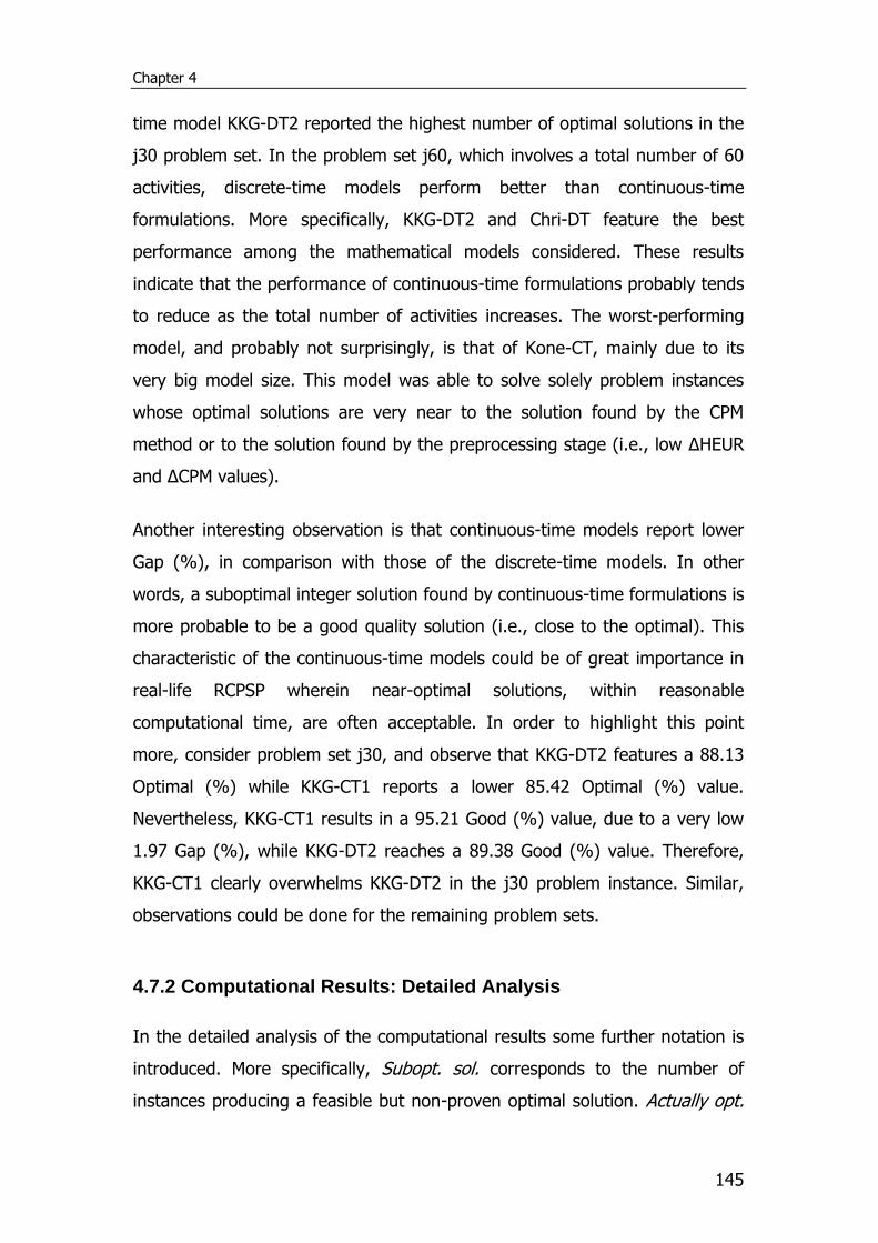
Chapter 4
145
time model KKG-DT2 reported the highest number of optimal solutions in the
j30 problem set. In the problem set j60, which involves a total number of 60
activities, discrete-time models perform better than continuous-time
formulations. More specifically, KKG-DT2 and Chri-DT feature the best
performance among the mathematical models considered. These results
indicate that the performance of continuous-time formulations probably tends
to reduce as the total number of activities increases. The worst-performing
model, and probably not surprisingly, is that of Kone-CT, mainly due to its
very big model size. This model was able to solve solely problem instances
whose optimal solutions are very near to the solution found by the CPM
method or to the solution found by the preprocessing stage (i.e., low ΔHEUR
and ΔCΡΜ values).
Another interesting observation is that continuous-time models report lower
Gap (%), in comparison with those of the discrete-time models. In other
words, a suboptimal integer solution found by continuous-time formulations is
more probable to be a good quality solution (i.e., close to the optimal). This
characteristic of the continuous-time models could be of great importance in
real-life RCPSP wherein near-optimal solutions, within reasonable
computational time, are often acceptable. In order to highlight this point
more, consider problem set j30, and observe that KKG-DT2 features a 88.13
Optimal (%) while KKG-CT1 reports a lower 85.42 Optimal (%) value.
Nevertheless, KKG-CT1 results in a 95.21 Good (%) value, due to a very low
1.97 Gap (%), while KKG-DT2 reaches a 89.38 Good (%) value. Therefore,
KKG-CT1 clearly overwhelms KKG-DT2 in the j30 problem instance. Similar,
observations could be done for the remaining problem sets.
4.7.2 Computational Results: Detailed Analysis
In the detailed analysis of the computational results some further notation is
introduced. More specifically, Subopt. sol. corresponds to the number of
instances producing a feasible but non-proven optimal solution. Actually opt.
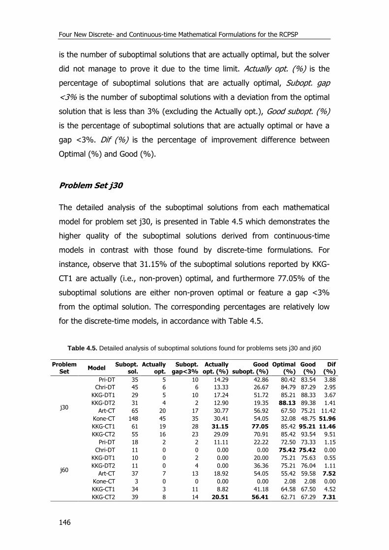
Four New Discrete- and Continuous-time Mathematical Formulations for the RCPSP
146
is the number of suboptimal solutions that are actually optimal, but the solver
did not manage to prove it due to the time limit. Actually opt. (%) is the
percentage of suboptimal solutions that are actually optimal, Subopt. gap
<3% is the number of suboptimal solutions with a deviation from the optimal
solution that is less than 3% (excluding the Actually opt.), Good subopt. (%)
is the percentage of suboptimal solutions that are actually optimal or have a
gap <3%. Dif (%) is the percentage of improvement difference between
Optimal (%) and Good (%).
Problem Set j30
The detailed analysis of the suboptimal solutions from each mathematical
model for problem set j30, is presented in Table 4.5 which demonstrates the
higher quality of the suboptimal solutions derived from continuous-time
models in contrast with those found by discrete-time formulations. For
instance, observe that 31.15% of the suboptimal solutions reported by KKG-
CT1 are actually (i.e., non-proven) optimal, and furthermore 77.05% of the
suboptimal solutions are either non-proven optimal or feature a gap <3%
from the optimal solution. The corresponding percentages are relatively low
for the discrete-time models, in accordance with Table 4.5.
Table 4.5. Detailed analysis of suboptimal solutions found for problems sets j30 and j60
Problem Set
Model Subopt.
sol. Actually
opt. Subopt.
gap<3% Actually
opt. (%) Good
subopt. (%) Optimal
(%) Good (%)
Dif (%)
j30
Pri-DT 35 5 10 14.29 42.86 80.42 83.54 3.88
Chri-DT 45 6 6 13.33 26.67 84.79 87.29 2.95
KKG-DT1 29 5 10 17.24 51.72 85.21 88.33 3.67
KKG-DT2 31 4 2 12.90 19.35 88.13 89.38 1.41
Art-CT 65 20 17 30.77 56.92 67.50 75.21 11.42
Kone-CT 148 45 35 30.41 54.05 32.08 48.75 51.96
KKG-CT1 61 19 28 31.15 77.05 85.42 95.21 11.46
KKG-CT2 55 16 23 29.09 70.91 85.42 93.54 9.51
j60
Pri-DT 18 2 2 11.11 22.22 72.50 73.33 1.15
Chri-DT 11 0 0 0.00 0.00 75.42 75.42 0.00
KKG-DT1 10 0 2 0.00 20.00 75.21 75.63 0.55
KKG-DT2 11 0 4 0.00 36.36 75.21 76.04 1.11
Art-CT 37 7 13 18.92 54.05 55.42 59.58 7.52
Kone-CT 3 0 0 0.00 0.00 2.08 2.08 0.00
KKG-CT1 34 3 11 8.82 41.18 64.58 67.50 4.52
KKG-CT2 39 8 14 20.51 56.41 62.71 67.29 7.31
Chapter 4
147
Table 4.6 shows a detailed analysis of good quality solutions for different RS
and RF parameter settings for problem set j30. The maximum value for each
cell is 30 instances. This also applies to Tables 4.7 and 4.8. According to this
table, problem instances with low RS value (i.e., 0.20) and high RF values
(i.e., 0.75, and 1.00) are the most difficult RCPSP to solve by the
mathematical models considered. Note that only the proposed KKG-CT1 and
KKG-CT2 models have managed to solve a significant percentage of these
problem instances. The most difficult problem instances for KKG-CT1 and
KKG-CT2 are those with RS={0.20, 0.50} and RF=1.00. It should be noted
that discrete-time models solved almost all problems with RS=0.50 and
RF=1.00, but manage to solve just a very small number of problem instances
with RS=0.20 and RF={0.75, 1.00}. The majority of the remaining problem
instances in problem set j30 have been solved by the mathematical models
considered except for the Kone-CT model, which performed poorly. The
proposed KKG-CT1 formulation found the most good quality solutions,
resulting into a 95.21% good solutions percentage.
Table 4.6. Detailed analysis of good quality solutions per RS and RF parameter setting for
j30
Parameter Mathematical Formulation
RS RF Pri-DT Chri-DT KKG-DT1 KKG-DT2 Art-CT Kone-CT KKG-CT1 KKG-CT2
0.20 0.25 30 30 30 30 30 16 30 30
0.20 0.50 14 23 27 30 8 8 30 30
0.20 0.75 0 4 6 7 0 1 29 27
0.20 1.00 0 6 3 2 0 2 23 18
0.50 0.25 30 30 30 30 30 19 30 30
0.50 0.50 30 30 30 30 29 11 30 30
0.50 0.75 30 30 30 30 23 6 28 28
0.50 1.00 27 26 28 30 4 2 18 19
0.70 0.25 30 30 30 30 30 26 30 30
0.70 0.50 30 30 30 30 30 14 30 30
0.70 0.75 30 30 30 30 30 12 30 30
0.70 1.00 30 30 30 30 27 10 29 27
1.00 0.25 30 30 30 30 30 29 30 30
1.00 0.50 30 30 30 30 30 28 30 30
1.00 0.75 30 30 30 30 30 24 30 30
1.00 1.00 30 30 30 30 30 26 30 30
Good solutions 401 419 424 429 361 234 457 449
Good (%) 83.54 87.29 88.33 89.38 75.21 48.75 95.21 93.54
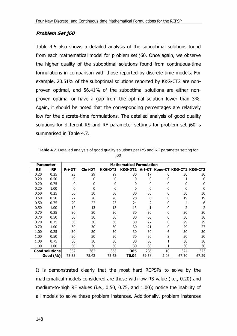
Four New Discrete- and Continuous-time Mathematical Formulations for the RCPSP
148
Problem Set j60
Table 4.5 also shows a detailed analysis of the suboptimal solutions found
from each mathematical model for problem set j60. Once again, we observe
the higher quality of the suboptimal solutions found from continuous-time
formulations in comparison with those reported by discrete-time models. For
example, 20.51% of the suboptimal solutions reported by KKG-CT2 are non-
proven optimal, and 56.41% of the suboptimal solutions are either non-
proven optimal or have a gap from the optimal solution lower than 3%.
Again, it should be noted that the corresponding percentages are relatively
low for the discrete-time formulations. The detailed analysis of good quality
solutions for different RS and RF parameter settings for problem set j60 is
summarised in Table 4.7.
Table 4.7. Detailed analysis of good quality solutions per RS and RF parameter setting for
j60
Parameter Mathematical Formulation
RS RF Pri-DT Chri-DT KKG-DT1 KKG-DT2 Art-CT Kone-CT KKG-CT1 KKG-CT2
0.20 0.25 23 29 29 30 17 0 30 30
0.20 0.50 0 0 0 0 0 0 1 0
0.20 0.75 0 0 0 0 0 0 0 0
0.20 1.00 0 0 0 0 0 0 0 0
0.50 0.25 30 30 30 30 30 0 30 30
0.50 0.50 27 28 28 28 8 0 19 19
0.50 0.75 20 22 23 24 2 0 4 6
0.50 1.00 12 13 13 13 1 0 2 2
0.70 0.25 30 30 30 30 30 0 30 30
0.70 0.50 30 30 30 30 30 0 30 30
0.70 0.75 30 30 30 30 27 0 29 29
0.70 1.00 30 30 30 30 21 0 29 27
1.00 0.25 30 30 30 30 30 6 30 30
1.00 0.50 30 30 30 30 30 2 30 30
1.00 0.75 30 30 30 30 30 1 30 30
1.00 1.00 30 30 30 30 30 1 30 30
Good solutions 352 362 363 365 286 10 324 323
Good (%) 73.33 75.42 75.63 76.04 59.58 2.08 67.50 67.29
It is demonstrated clearly that the most hard RCPSPs to solve by the
mathematical models considered are those with low RS value (i.e., 0.20) and
medium-to-high RF values (i.e., 0.50, 0.75, and 1.00); notice the inability of
all models to solve these problem instances. Additionally, problem instances
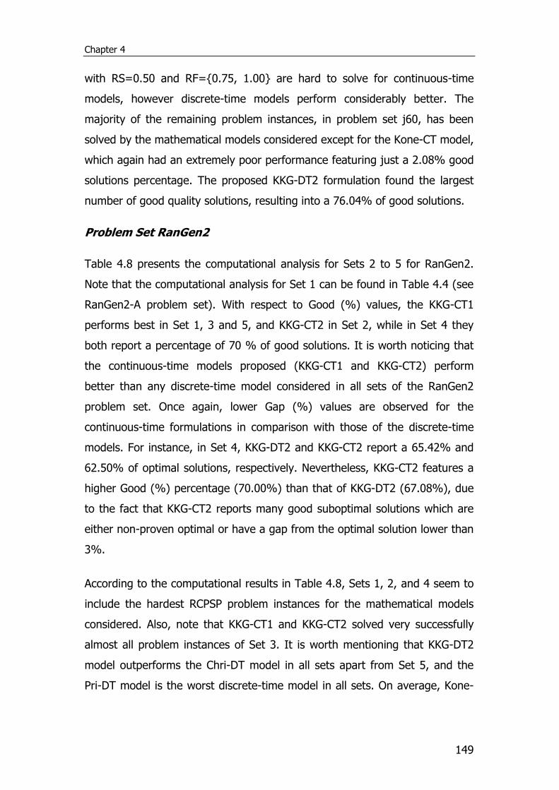
Chapter 4
149
with RS=0.50 and RF={0.75, 1.00} are hard to solve for continuous-time
models, however discrete-time models perform considerably better. The
majority of the remaining problem instances, in problem set j60, has been
solved by the mathematical models considered except for the Kone-CT model,
which again had an extremely poor performance featuring just a 2.08% good
solutions percentage. The proposed KKG-DT2 formulation found the largest
number of good quality solutions, resulting into a 76.04% of good solutions.
Problem Set RanGen2
Table 4.8 presents the computational analysis for Sets 2 to 5 for RanGen2.
Note that the computational analysis for Set 1 can be found in Table 4.4 (see
RanGen2-A problem set). With respect to Good (%) values, the KKG-CT1
performs best in Set 1, 3 and 5, and KKG-CT2 in Set 2, while in Set 4 they
both report a percentage of 70 % of good solutions. It is worth noticing that
the continuous-time models proposed (KKG-CT1 and KKG-CT2) perform
better than any discrete-time model considered in all sets of the RanGen2
problem set. Once again, lower Gap (%) values are observed for the
continuous-time formulations in comparison with those of the discrete-time
models. For instance, in Set 4, KKG-DT2 and KKG-CT2 report a 65.42% and
62.50% of optimal solutions, respectively. Nevertheless, KKG-CT2 features a
higher Good (%) percentage (70.00%) than that of KKG-DT2 (67.08%), due
to the fact that KKG-CT2 reports many good suboptimal solutions which are
either non-proven optimal or have a gap from the optimal solution lower than
3%.
According to the computational results in Table 4.8, Sets 1, 2, and 4 seem to
include the hardest RCPSP problem instances for the mathematical models
considered. Also, note that KKG-CT1 and KKG-CT2 solved very successfully
almost all problem instances of Set 3. It is worth mentioning that KKG-DT2
model outperforms the Chri-DT model in all sets apart from Set 5, and the
Pri-DT model is the worst discrete-time model in all sets. On average, Kone-
Four New Discrete- and Continuous-time Mathematical Formulations for the RCPSP
150
CT performs better than Art-CT in contrast with the previous problem sets j30
and j60.
Table 4.8. Computational analysis for problem Set 2 to 5 for RanGen2
Problem Set
Model Feasible
(%) Good (%)
Optimal (%)
Gap (%)
ΔHEUR (%)
ΔCPM (%)
Optimal CPU s
Set 2
Pri-DT 64.44 52.22 49.44 13.02 6.46 5.77 34.14
Chri-DT 77.78 54.44 54.44 11.79 6.39 7.48 19.50
KKG-DT1 78.33 56.11 52.78 12.06 6.48 6.97 37.96
KKG-DT2 83.89 56.67 55.56 12.81 6.40 7.93 30.42
Art-CT 26.11 23.33 16.11 2.69 2.33 8.91 31.02
Kone-CT 67.78 46.67 18.89 4.51 5.18 2.11 105.26
KKG-CT1 80.56 61.67 53.33 6.44 5.92 10.08 17.23
KKG-CT2 81.67 64.44 55.00 7.06 6.24 9.79 27.86
Set 3
Pri-DT 67.92 64.17 58.75 3.88 0.66 10.71 13.81
Chri-DT 81.25 71.67 67.92 5.50 0.91 13.17 18.76
KKG-DT1 74.58 69.58 65.83 5.71 0.87 12.89 36.39
KKG-DT2 81.25 72.50 70.00 7.50 1.02 14.06 28.61
Art-CT 70.00 67.08 62.92 2.30 0.73 11.76 22.86
Kone-CT 91.25 79.17 33.75 1.73 0.25 4.69 13.06
KKG-CT1 99.17 94.58 81.25 2.01 1.69 22.16 22.64
KKG-CT2 98.33 94.17 81.25 2.44 1.72 21.72 20.15
Set 4
Pri-DT 75.00 62.50 60.00 9.68 4.88 3.58 27.06
Chri-DT 86.25 66.67 64.17 9.77 5.29 4.30 16.13
KKG-DT1 86.25 67.50 63.33 11.54 5.26 4.13 30.47
KKG-DT2 86.67 67.08 65.42 11.54 5.37 4.64 16.65
Art-CT 42.92 39.17 30.00 2.94 2.03 1.81 23.36
Kone-CT 76.25 57.92 32.08 4.02 3.12 1.05 52.59
KKG-CT1 83.75 70.00 63.33 6.14 4.94 5.65 21.38
KKG-CT2 83.75 70.00 62.50 5.30 4.79 4.68 12.43
Set 5
Pri-DT 74.58 64.58 61.67 10.57 4.47 3.74 23.91
Chri-DT 85.42 67.92 66.67 11.41 4.84 4.71 14.40
KKG-DT1 83.75 67.50 66.25 11.63 4.79 4.62 31.75
KKG-DT2 87.92 67.08 66.67 12.67 4.84 4.71 13.02
Art-CT 47.50 43.33 32.92 2.50 2.45 1.86 28.89
Kone-CT 76.25 59.17 32.08 3.97 2.79 0.51 35.53
KKG-CT1 91.25 74.17 67.92 6.52 4.96 7.22 19.13
KKG-CT2 88.75 72.92 67.08 5.84 4.90 7.03 12.87
4.8 Conclusions
This chapter presents two BIP discrete-time models (KKG-DT1, KKG-DT2) and
two MIP continuous-time formulations (KKG-CT1, KKG-CT2) followed by a
detailed comparison with four existing literature models using 2760 RCPSPs.
Overall, KKG-CT1 and KKG-CT2 have been found to be the best models for
Chapter 4
151
the problems addressed. The detailed and comprehensive computational
analysis reveals some interesting features of the problems solved and the
mathematical models considered. More specifically, it has been observed, that
problem instances with low RS values and high RF values are the most hard
to solve, according to the computational results in problem sets j30 and j60.
Moreover, it seems that increasing the number of activities directly affects
negatively the computational performance of continuous-time models since
the number of sequencing binary variables is increased dramatically, while
discrete-time models are affected less due to the fact that the number of the
decisions variables principally depends on the time points. Notice that, in
contrast to continuous-time models, the performance of discrete-time models
is strongly affected (positively) from the bounds imposed on the
preprocessing phase. In addition, continuous-time formulations feature lower
Gap (%) values compared with discrete-time models. Also, the event-based
Kone-CT formulation generally performs poor and becomes inappropriate for
large number of activities due to the huge model size. Finally, it has been
demonstrated that continuous-time models, which have received little
attention in the literature so far, could deal very successfully and efficiently
with RCPSPs.
At this point, it should be emphasised that in discrete-time approaches: (a)
the scheduling horizon is divided into a finite number of time intervals with
predefined duration, and therefore (b) activities can start or end only at the
boundaries of these time periods. For this reason, in real-world problems
where the duration of the activities may not be integer numbers, a finer
division of the scheduling horizon (resulting in bigger model sizes), and/or
duration time rounding (sacrificing optimality) should be employed. An
inherent special advantage of continuous-time approaches is that timing
decisions can be represented explicitly. However, the modelling of resource
limitations needs more complicated constraints involving many big-M terms,
which tends to increase the model complexity.
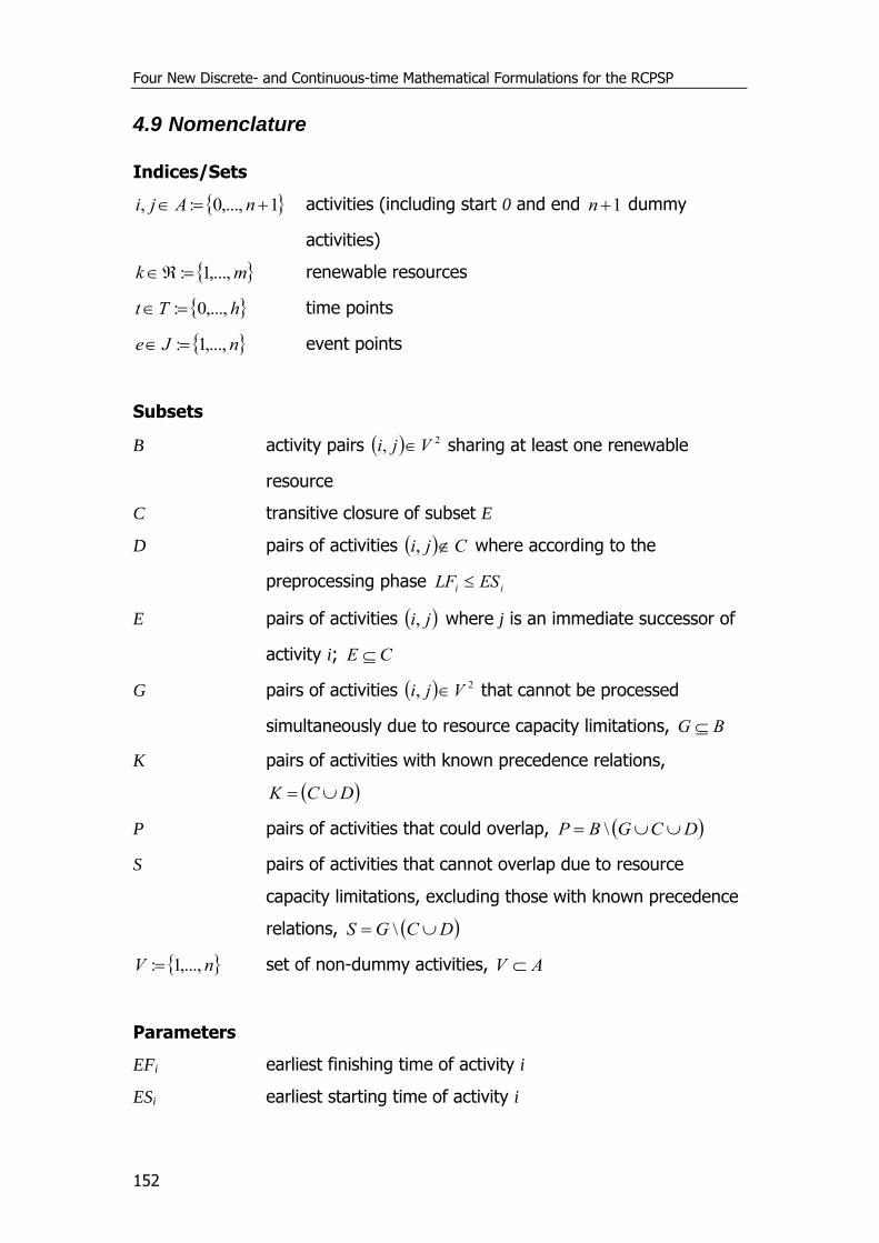
Four New Discrete- and Continuous-time Mathematical Formulations for the RCPSP
152
4.9 Nomenclature
Indices/Sets
1,...,0:, nAji activities (including start 0 and end 1n dummy
activities)
mk ,...,1: renewable resources
hTt ,...,0: time points
nJe ,...,1: event points
Subsets
B activity pairs 2, Vji sharing at least one renewable
resource
C transitive closure of subset E
D pairs of activities Cji , where according to the
preprocessing phase ii ESLF
E pairs of activities ji, where j is an immediate successor of
activity i; CE
G pairs of activities 2, Vji that cannot be processed
simultaneously due to resource capacity limitations, BG
K pairs of activities with known precedence relations,
DCK
P pairs of activities that could overlap, DCGBP \
S pairs of activities that cannot overlap due to resource
capacity limitations, excluding those with known precedence
relations, DCGS \
nV ,...,1: set of non-dummy activities, AV
Parameters
EFi earliest finishing time of activity i
ESi earliest starting time of activity i
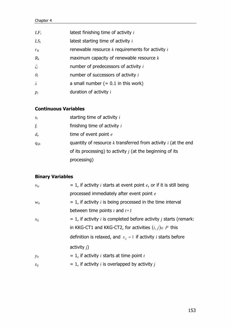
Chapter 4
153
LFi latest finishing time of activity i
LSi latest starting time of activity i
rik renewable resource k requirements for activity i
Rk maximum capacity of renewable resource k
ζi number of predecessors of activity i
θi number of successors of activity i
λ a small number (= 0.1 in this work)
pi duration of activity i
Continuous Variables
si starting time of activity i
fi finishing time of activity i
de time of event point e
qijk quantity of resource k transferred from activity i (at the end
of its processing) to activity j (at the beginning of its
processing)
Binary Variables
vie = 1, if activity i starts at event point e, or if it is still being
processed immediately after event point e
wit = 1, if activity i is being processed in the time interval
between time points t and t+1
xij = 1, if activity i is completed before activity j starts (remark:
in KKG-CT1 and KKG-CT2, for activities Pji , this
definition is relaxed, and 1ijx if activity i starts before
activity j)
yit = 1, if activity i starts at time point t
zij = 1, if activity i is overlapped by activity j

154
Chapter 5
155
Chapter 5
Mathematical Formulation for Resource-
Constrained Project Scheduling Problems with
Generalised Precedence Relations
This chapter presents a new precedence-based continuous-time formulation
for a challenging extension of the standard single-mode resource-constrained
project scheduling problem that also considers minimum and maximum time
lags (RCPSP/max), under the objective of minimizing the project makespan.
The proposed linear mixed integer programming model is based on the
definition of two types of binary variables to express: (i) the relative
sequencing of activities, and (ii) the overlapping conditions. Two types of
continuous variables for activity starting and finishing times are also used.
Additionally, a number of new activity subsets are introduced for modelling
purposes, in order to reduce the model size and tighten the proposed model.
The new mathematical formulation is used to conduct an extensive
computational study on a total of 2,250 well-known and open-accessed
benchmark problem instances from the literature. Various problem sizes are
considered in the test sets involving 10, 20, 30, 50 and 100 activities. The
computational results illustrate the efficient performance of the proposed
mathematical formulation. Finally, interesting observations are made through
the computational study and potential future research lines are proposed.
5.1 Introduction
The classical single-mode RCPSP uses finish-start precedence relations with
zero time-lags, which means that an activity can only start as soon as all its
predecessor activities have finished. This work studies a challenging
Mathematical Formulation for the RCPSP/max
156
extension of the RCPSP in which activity starting times are constrained by
generalised precedence relations (also called temporal constraints or
minimum and maximum time lags or time windows). This extension is
denoted as RCPSP/max or PS | temp | Cmax, using the notation of Brucker et al.
(1999). More specifically, PS | temp | Cmax notation specifies the single-mode
project scheduling problem (PS) under general temporal constraints given by
minimum and maximum start-start time lags between activities (temp) while
minimizing the makespan of the project (Cmax).
Elmaghraby and Kamburowski (1992) defined four types of generalised
precedence relations (GPR): Start-Start (SS), Start-Finish (SF), Finish-Start
(FS) and Finish-Finish (FF) to model minimum and maximum time-lags. For
activity pairs ji, , the minimum time-lag ( xSSijmin , xSFij
min , xFFijmin ,
xFS ijmin ) specifies that activity j can only start/finish when its predecessor i
has already started/finished for a certain x time period (in time units). A
maximum time-lag ( xSSijmax , xSFij
max , xFFijmax , xFS ij
max ) specifies that
activity j should start/finish at the latest x time periods after the start/finish of
activity i. The various types of GPRs can be represented in a standardised
form by reducing them to minimum SS precedence relationships, through the
transformations proposed by Bartusch et al. (1988).
From a modelling point of view, time lags are necessary to represent partial
or total overlapping of activities, release or ready times, project milestones
and deadlines, time windows or time-varying resource requirements. For even
more applications of GPRs to modelling real-life project scheduling problems,
we refer the reader to Neumann and Schwindt (1995).
The addition of maximal time lags to the classical RCPSP, significantly
increases the complexity of the problem. Moreover, the generation of
problem instances could be problematic because infeasible problems might be
generated. The RCPSP/max is an NP-hard problem and even the theoretically
Chapter 5
157
easier problem of checking its feasibility is NP-complete (Hartmann and
Briskorn, 2010).
The main contribution of this chapter is that it efficiently solves the
RCPSP/max using a pure mathematical programming approach. It is an
extension of the KKG-CT2 model introduced in the previous chapter, and to
the best of our knowledge, it is the only continuous-time approach for the
RCPSP/max, in the OR literature. The only other mathematical model for the
RCPSP/max is proposed Bianco and Caramia (2012b), but it is a discrete-time
one. The formulation is used to calculate a lower bound through a
Langrangean relaxation and a branch-and-bound algorithm which exploits
both.
The rest of the chapter is organised as follows. In Section 5.2, the
RCPSP/max problem is formally stated. Section 5.3 describes the
preprocessing phase employed in this work. Section 5.4 describes in detail
the new continuous-time Mixed-Integer Programming (MIP) formulation. A
brief description of the problem instance sets considered and a
comprehensive computational study are presented in Section 5.5. Finally,
concluding remarks are drawn in Section 5.6.
5.2 Problem statement
The single-mode RCPSP/max consists of a set of n activities nV ,...,1 , that
have to be processed without interruption, under the objective of minimising
the project makespan. For modelling purposes, dummy activities 0 and n+1 to
represent the beginning and completion of the project are defined. Set
1,,...,1,0 nnA defines the new complete set of activities. The processing
time of activity i is denoted by ip , (for dummy activities 010 npp ).
The project utilises a set of renewable resource types mk ,...,1: . Each
activity i requires ikr units of resource k during each time period of its
Mathematical Formulation for the RCPSP/max
158
execution ( 0,10 knk rr ). The maximum available capacity of each resource
k is kR units. Renewable resources fully retrieve the occupied resource
amount after the completion of each activity. In other words, the temporary
availability of the renewable resources at every time is constrained.
Modelling activities with a piecewise constant resource requirement trik
(i.e., activity i requires an amount )(trik of resource k , during the t th
time unit it is in process) can be easily done by replacing them with several
other activities which are “tied together” through temporal constraints.
Similarly, time-varying resource availability )(tRk (i.e., a specific quantity
)(tRk of resource k is available at time t) can be modelled by introducing
dummy jobs with fixed start times which consume excessive resources.
Therefore, it is safe to assume that )(trik and )(tRk are constant over time
without any loss of generality (Fest et al., 1998).
Time lags ijd between activity pairs ),( ji are included in set E and take
integer values (i.e., ijd ). Time lags can be presented as an activity-on-
node (AON) network dEAG ,, , where nodes correspond to the set of
activities A and set E represents the arcs with weight d. Minimal lags are
usually represented as forward arcs and maximal lags as backward arcs.
Given that the various types of minimum and maximum time lags (SS, SF, FS,
FF) can be transformed to a single type using the rules by Bartusch et al.
(1988), from now on we will consider them to be of type start-start. Time
lags can be represented in the following general form:
iijj sds Eji ,
where is ( js ) is the starting time of activity i ( j ). The case 0ijd
corresponds to a minimum time lag of ijd units, stating that activity j has to
start at least ijd time units after the start time of activity i. The case 0ijd
Chapter 5
159
corresponds to maximum time lag units, stating that activity i has to start at
the latest ijd time units after the start time of activity j. By exploiting time
lags, we can define a set L containing pairs of activities ji, that have real
precedence relations (i.e., the finishing time of activity i is smaller or equal to
the starting time of j). Specifically, when iij pd holds, activity j cannot
begin earlier than the finish of activity i ( iii fps , with if the finishing
time of activity i).
A solution for the RCPSP/max is a list of start times or schedule S = ( 0s , 1s , …,
ns , 1ns ), where 00 s , and 1ns corresponds to the makespan of the project.
5.3 Preprocessing
In this chapter some fast computable bounds are considered, however other
bounding techniques could be used. First, a trivial upper bound UB equal to
Ai
ijEji
i dp,max,max is calculated.
Defining an earliest starting time ( iES ) for each activity i is also a common
preprocessing step. It can be computed using the first of the Special
Implementations of the Modified Label Correcting Algorithm of Ahuja et al.
(1993); which is of EAO time complexity. A label correcting algorithm is
iterative and assigns tentative distance labels j to nodes at each step. The
distance labels are estimates of (i.e., lower bounds on) the longest path
distances and are considered as temporary until the final step where j is
the longest path length from the source node 1 to node j. In each pass, arcs
Eji , are scanned one by one, and condition ijij d is checked. If the
arc satisfies this condition, ijij d is updated. The algorithm stops when
Mathematical Formulation for the RCPSP/max
160
no distance label changes during an entire pass. Finally, we set jjES .
The algorithm runs as displayed in Algorithm 1.
Algorithm 1. Modified label-correcting algorithm
algorithm modified label-correcting;
begin
0:0 and 0:0 pred ;
:j for each node 0 Aj ;
falsenochange : ;
while truenochange do
begin
truenochange : ;
for each Ejiarc , do
begin
if ijij d then
begin
ijij d ;
falsenochange : ;
end;
end;
end;
end;
Through the iES we can easily calculate the earliest finishing times iEF by
adding the activity duration ( iii pESEF ). We can also set a trivial lower
bound to the time horizon, equal to the earliest finishing time of the dummy
end activity ( 1 nEFLB ). It should be noted that other preprocessing
methods could be used, potentially yielding better bounds at the expense of
CPU time. Here we have chosen a relatively simple method that requires
negligible computational effort.
Chapter 5
161
5.4 The mathematical model
The proposed MIP mathematical formulation relies on a continuous-time
approach. Binary sequencing variables are defined to represent activity
ordering and overlapping, and continuous variables are used for activity
starting and finishing times. The presented formulation is an extension of the
KKG-CT2 model introduced in the previous chapter. For projects that contain
activities with non-integer durations, continuous-time formulations are more
efficient than discrete-time formulations. In the proposed approach,
continuous variables is , if defined for each activity 1 nVi , denote
its starting and finishing time, while binary sequencing variables ijx define the
relative execution order of activities i and j. For pairs of activities that cannot
be executed in parallel (e.g., activities for which the sum of resource
requirements exceeds the maximum availability, etc), 1ijx if activity i is
completed before activity j starts processing (i.e., ji sf ) , otherwise is 0.
However, for pair of activities that could execute in parallel, ijx is used to
define the relative sequencing between the activities' starting times. More
specifically, 1ijx if activity i begins processing before (i.e., ji ss ), or
exactly at the same time as activity j starts and j has a larger index (i.e.,
ji ss with ji ), otherwise is equal to 0.
In order to model renewable resource constraints, pairs of activities that
could be executed in parallel should be defined. That can be done by
extending the concept of overlapping activities (Marchetti and Cerdá, 2009).
By definition, an activity j that is overlapping the starting time of activity i
must satisfy the following conditions (see Fig. 5.1):
A) it should require at least one resource k in common with activity i (i.e.,
0ikr and 0jkr ),
B) it starts before or exactly at the time that activity i starts processing
(i.e., ij ss ) and
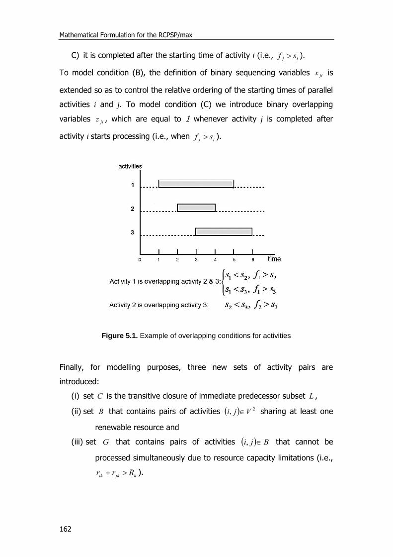
Mathematical Formulation for the RCPSP/max
162
C) it is completed after the starting time of activity i (i.e., ij sf ).
To model condition (B), the definition of binary sequencing variables jix is
extended so as to control the relative ordering of the starting times of parallel
activities i and j. To model condition (C) we introduce binary overlapping
variables jiz , which are equal to 1 whenever activity j is completed after
activity i starts processing (i.e., when ij sf ).
Figure 5.1. Example of overlapping conditions for activities
Finally, for modelling purposes, three new sets of activity pairs are
introduced:
(i) set C is the transitive closure of immediate predecessor subset L ,
(ii) set B that contains pairs of activities 2, Vji sharing at least one
renewable resource and
(iii) set G that contains pairs of activities Bji , that cannot be
processed simultaneously due to resource capacity limitations (i.e.,
kjkik Rrr ).

Chapter 5
163
Two more composite sets are defined by using the previously defined sets of
activities. The first set CGS \ contains pairs of activities that cannot
overlap due to resource capacity limitations, excluding those with known
precedence relations. Notice that for this set only variables ijx need to be
defined. And the second set CGBP \ contains pairs of activities that
could overlap. For such activity pairs, both ijx and jiz variables need to be
defined. The preprocessing time to determine sets B, C, G, L, P and S is
negligible. Using the above definition of sets and decision variables, the
following mathematical formulation is proposed:
1maxmin nfC (1)
00 s (2)
iii psf 1 nVi (3)
ji sf CjinVjVi ,:1, (4)
iijj sds Eji , (5)
jiiij xESMsf 1 jiSji :, (6)
jijji xESMsf jiSji :, (7)
jiiij xESMss 1 jiPji :, (8)
jijji xESMss jiPji :, (9)
jiiij zESMsf jiPji :, (10)
kijjijk
Pji
rij
jijijk
Pji
rij
ik Rxzrxzrrjkjk
,
0:
,
0:
1 0:, ikrRkVi (11)
ijji zx jiPji :, (12)
jiji zx 1 jiPji :, (13)
1,0jix jiSPji :,
1,0jiz jiPji :, (14)
iiii EFfESs , 1 nVi
Mathematical Formulation for the RCPSP/max
164
Equation (1) minimises the completion time of dummy end activity n+1,
representing the project completion. Note that the makespan is lower than or
equal to the upper bound UB calculated in the preprocessing phase. The
starting time of the dummy start activity is equal to zero, according to
constraint (2). Constraints (3) correlate the starting and finishing times for
activities 1 nVi throughout their execution. Constraints (4) set all a
priori known precedence relations between activities Cji , , through their
starting and finishing times. Minimum and maximum time lags ijd are
imposed by constraints (5). Big-M constraints (6) to (9) define the sequencing
constraints between any pair of activities Cji , when ji . The value of
big M parameters could strongly affect the performance of any model. For
this reason, and in order not to use any arbitrary values for the big M
parameters, a value equal to UB+1 is used, the trivial upper bound to the
time horizon, calculated in Section 5.3. To reduce the solution search space,
the value of the big M parameters is properly adjusted by the ES of the
corresponding activity. It should be noted that constraints (8) and (9) extend
the definition of sequencing binary variable ijx to also control the starting
times of the parallel tasks i and j. Also, notice that a small positive parameter
ι is included to constraint (9) so as to deal with the case that activities i and j
start processing at the same time. That way, when ji ss the activity with
the higher index is assumed to start last (i.e., if ji ss and ji , then
1jix ). In the case studies, parameter 1.0 . Overlapping condition (C) is
modelled by constraints (10), and renewable resource constraints are given
by constraints (11). By splitting the resource demand into two separate
summations containing 1 jiji xz when ij and ijji xz when ij , we
are able to detect overlapping between activity pairs Pji , and properly
model the resource constraints.
Constraints (8) to (11) state that if activity i starts processing before activity j
(i.e., 1ijx ), then activity j has to finish after activity i starts (i.e., 1jiz ).

Chapter 5
165
The only case that one of the parentheses 1 jiji xz and ijji xz in the
resource constraints (10) takes the value of 1 is when activity j overlaps i
(i.e., 1jiz ) and activity j starts processing before i (i.e., 1jix ). It can be
easily proven that for activities which could overlap Pji , , if 1ijx that
means that jji fss , and consequently 0 ij sf which according to
constraints (10) gives 1jiz . Table 5.1 displays all possible combinations for
variables jiz and ijx for activities Pji , that could be executed in parallel.
In the first two cases wherein 0jiz , no overlapping occurs since activity i
starts after the completion of activity j (i.e., ijj sfs ). Especially, in the
second case, notice that if 0jiz , 1ijx and 0jix that would mean that
jij ssf , which is obviously impossible. For this reason, if 0jiz then
always 0ijx . In the last two cases wherein 1jiz , overlapping occurs if and
only if activity j begins processing before activity i starts (i.e., 0ijx ),
because in that case holds jij fss .
Table 5.1 Modelling of binary variables jiz and ijx for activities Pji ,
Constraints (10) Constraints (8) – (9) Constraints (11)
ij sf jiz ji ss ijx jix 1 jiji xz ijji xz
≤ 0 0 > 0 0 1 0 0
≤ 0 0 < 0 1 0 impossible impossible
> 0 1 < 0 1 0 0 0
> 0 1 > 0 0 1 1 1
Constraints (12) and (13) are tightening constraints that correlate directly
sequencing and overlapping binary variables. Finally, the domain of the
decision variables is given by constraints (14).
In summary, the proposed continuous-time MIP model for the RCPSP/max
consists of constraints (1) - (14).
Mathematical Formulation for the RCPSP/max
166
5.5 Computational Results
In this section we present the problem sets solved by the proposed
mathematical formulation and an extended computational study. All problem
instances have been solved on an Intel Core i5 CPU M430 2.27GHz with 4GB
RAM using CPLEX 11.1.1 via a GAMS 22.8.1 (Rosenthal, 2012) WIN
6007.6015 VIS interface under standard configurations. A maximum resource
time limit of 600 CPU s has been set for all problem instances.
5.6 Description of Problem Sets
Three widely-used test sets consisting of a total of 2,250 problem instances
have been solved by the proposed mathematical formulation. These sets
were generated by ProGen/max, a random networks generator by Schwindt
(1996) capable of creating project scheduling problems of varying structure,
constrainedness and difficulty. It is an extension of the instance generator
ProGen, developed by Kolisch and Sprecher (1996) which was designed to
create instances with ordinary precedence constraints only. It uses two
generating methods: DIRECT, which directly generates entire projects, and
CONTRACT, which first generates cycle structures, upon which the (acyclic)
contracted project network is generated. At this point, we point out that the
generator does not always produce instances with a feasible solution. These
instances are included in the computational study, since proving their
infeasibility is an NP-complete problem.
The first set was taken from Schwindt (1998a) and contains 270 problems for
each network size of 30,20,10n activities. These problem sets will be
referred to as j10, j20 and j30, for 30,20,10n respectively. The second set,
from Franck et al. [13] includes 90 instances for each network size with
100,50,20,10n . From now on, these test sets will be referred as ubo10,
ubo20, ubo50 and ubo100, depending on the number of activities. Finally, the
third set was generated by Schwindt (1996) and it contains 1080 instances
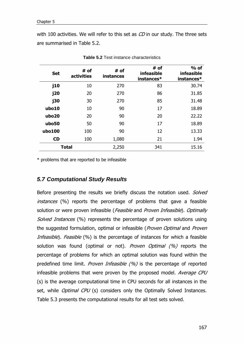
Chapter 5
167
with 100 activities. We will refer to this set as CD in our study. The three sets
are summarised in Table 5.2.
Table 5.2 Test instance characteristics
Set # of
activities # of
instances
# of infeasible
instances*
% of infeasible
instances*
j10 10 270 83 30.74
j20 20 270 86 31.85
j30 30 270 85 31.48
ubo10 10 90 17 18.89
ubo20 20 90 20 22.22
ubo50 50 90 17 18.89
ubo100 100 90 12 13.33
CD 100 1,080 21 1.94
Total 2,250 341 15.16
* problems that are reported to be infeasible
5.7 Computational Study Results
Before presenting the results we briefly discuss the notation used. Solved
instances (%) reports the percentage of problems that gave a feasible
solution or were proven infeasible (Feasible and Proven Infeasible). Optimally
Solved Instances (%) represents the percentage of proven solutions using
the suggested formulation, optimal or infeasible (Proven Optimal and Proven
Infeasible). Feasible (%) is the percentage of instances for which a feasible
solution was found (optimal or not). Proven Optimal (%) reports the
percentage of problems for which an optimal solution was found within the
predefined time limit. Proven Infeasible (%) is the percentage of reported
infeasible problems that were proven by the proposed model. Average CPU
(s) is the average computational time in CPU seconds for all instances in the
set, while Optimal CPU (s) considers only the Optimally Solved Instances.
Table 5.3 presents the computational results for all test sets solved.
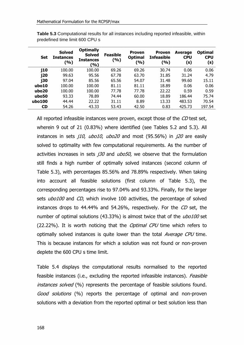
Mathematical Formulation for the RCPSP/max
168
Table 5.3 Computational results for all instances including reported infeasible, within
predefined time limit 600 CPU s
Set Solved
Instances (%)
Optimally Solved
Instances (%)
Feasible (%)
Proven Optimal
(%)
Proven Infeasible
(%)
Average CPU
(s)
Optimal CPU
(s)
j10 100.00 100.00 69.26 69.26 30.74 0.06 0.06
j20 99.63 95.56 67.78 63.70 31.85 31.24 4.79
j30 97.04 85.56 65.56 54.07 31.48 99.60 15.11
ubo10 100.00 100.00 81.11 81.11 18.89 0.06 0.06
ubo20 100.00 100.00 77.78 77.78 22.22 0.59 0.59
ubo50 93.33 78.89 74.44 60.00 18.89 186.44 75.74
ubo100 44.44 22.22 31.11 8.89 13.33 483.53 70.54
CD 54.26 43.33 53.43 42.50 0.83 425.73 197.54
All reported infeasible instances were proven, except those of the CD test set,
wherein 9 out of 21 (0.83%) where identified (see Tables 5.2 and 5.3). All
instances in sets j10, ubo10, ubo20 and most (95.56%) in j20 are easily
solved to optimality with few computational requirements. As the number of
activities increases in sets j30 and ubo50, we observe that the formulation
still finds a high number of optimally solved instances (second column of
Table 5.3), with percentages 85.56% and 78.89% respectively. When taking
into account all feasible solutions (first column of Table 5.3), the
corresponding percentages rise to 97.04% and 93.33%. Finally, for the larger
sets ubo100 and CD, which involve 100 activities, the percentage of solved
instances drops to 44.44% and 54.26%, respectively. For the CD set, the
number of optimal solutions (43.33%) is almost twice that of the ubo100 set
(22.22%). It is worth noticing that the Optimal CPU time which refers to
optimally solved instances is quite lower than the total Average CPU time.
This is because instances for which a solution was not found or non-proven
deplete the 600 CPU s time limit.
Table 5.4 displays the computational results normalised to the reported
feasible instances (i.e., excluding the reported infeasible instances). Feasible
instances solved (%) represents the percentage of feasible solutions found.
Good solutions (%) reports the percentage of optimal and non-proven
solutions with a deviation from the reported optimal or best solution less than
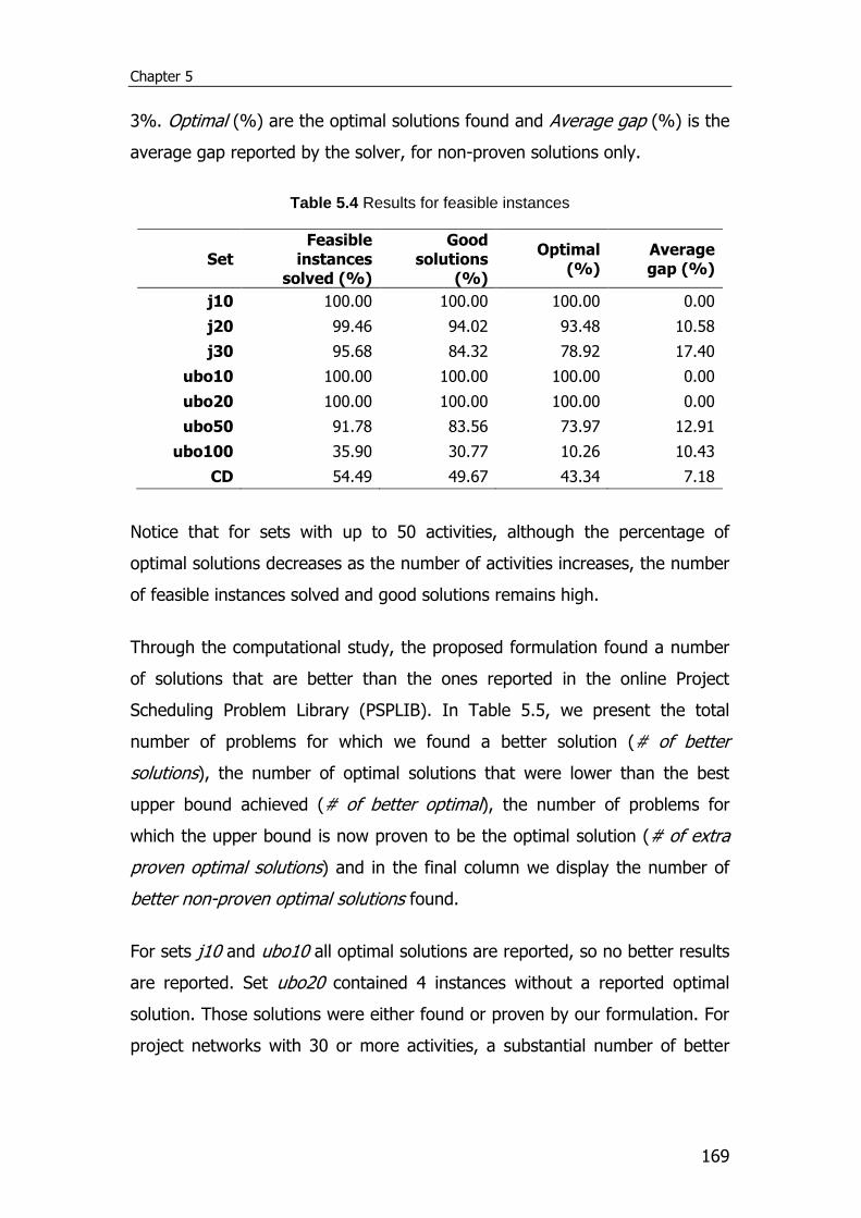
Chapter 5
169
3%. Optimal (%) are the optimal solutions found and Average gap (%) is the
average gap reported by the solver, for non-proven solutions only.
Table 5.4 Results for feasible instances
Set Feasible
instances solved (%)
Good solutions
(%)
Optimal (%)
Average gap (%)
j10 100.00 100.00 100.00 0.00
j20 99.46 94.02 93.48 10.58
j30 95.68 84.32 78.92 17.40
ubo10 100.00 100.00 100.00 0.00
ubo20 100.00 100.00 100.00 0.00
ubo50 91.78 83.56 73.97 12.91
ubo100 35.90 30.77 10.26 10.43
CD 54.49 49.67 43.34 7.18
Notice that for sets with up to 50 activities, although the percentage of
optimal solutions decreases as the number of activities increases, the number
of feasible instances solved and good solutions remains high.
Through the computational study, the proposed formulation found a number
of solutions that are better than the ones reported in the online Project
Scheduling Problem Library (PSPLIB). In Table 5.5, we present the total
number of problems for which we found a better solution (# of better
solutions), the number of optimal solutions that were lower than the best
upper bound achieved (# of better optimal), the number of problems for
which the upper bound is now proven to be the optimal solution (# of extra
proven optimal solutions) and in the final column we display the number of
better non-proven optimal solutions found.
For sets j10 and ubo10 all optimal solutions are reported, so no better results
are reported. Set ubo20 contained 4 instances without a reported optimal
solution. Those solutions were either found or proven by our formulation. For
project networks with 30 or more activities, a substantial number of better
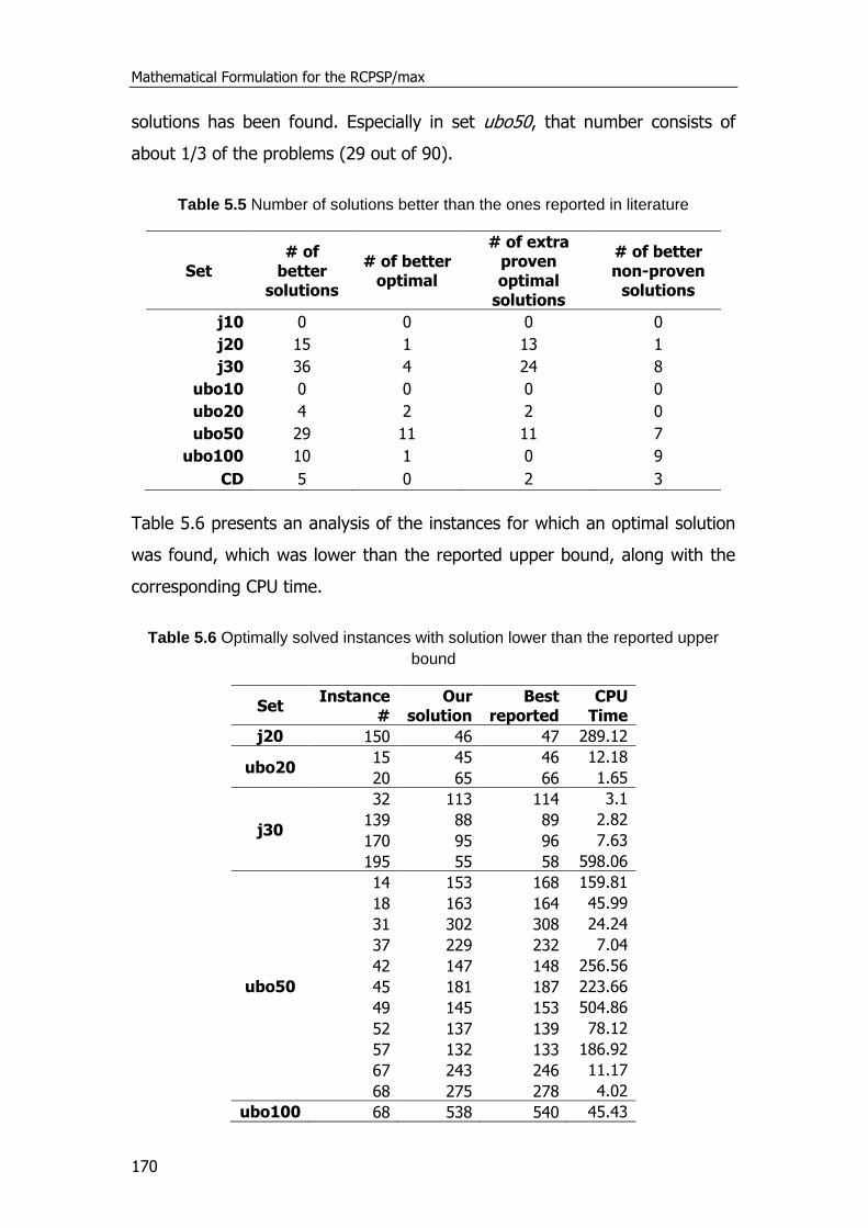
Mathematical Formulation for the RCPSP/max
170
solutions has been found. Especially in set ubo50, that number consists of
about 1/3 of the problems (29 out of 90).
Table 5.5 Number of solutions better than the ones reported in literature
Set # of
better solutions
# of better optimal
# of extra proven optimal
solutions
# of better non-proven
solutions
j10 0 0 0 0
j20 15 1 13 1
j30 36 4 24 8
ubo10 0 0 0 0
ubo20 4 2 2 0
ubo50 29 11 11 7
ubo100 10 1 0 9
CD 5 0 2 3
Table 5.6 presents an analysis of the instances for which an optimal solution
was found, which was lower than the reported upper bound, along with the
corresponding CPU time.
Table 5.6 Optimally solved instances with solution lower than the reported upper
bound
Set Instance
# Our
solution Best
reported CPU
Time
j20 150 46 47 289.12
ubo20 15 45 46 12.18
20 65 66 1.65
j30
32 113 114 3.1
139 88 89 2.82
170 95 96 7.63
195 55 58 598.06
ubo50
14 153 168 159.81
18 163 164 45.99
31 302 308 24.24
37 229 232 7.04
42 147 148 256.56
45 181 187 223.66
49 145 153 504.86
52 137 139 78.12
57 132 133 186.92
67 243 246 11.17
68 275 278 4.02
ubo100 68 538 540 45.43
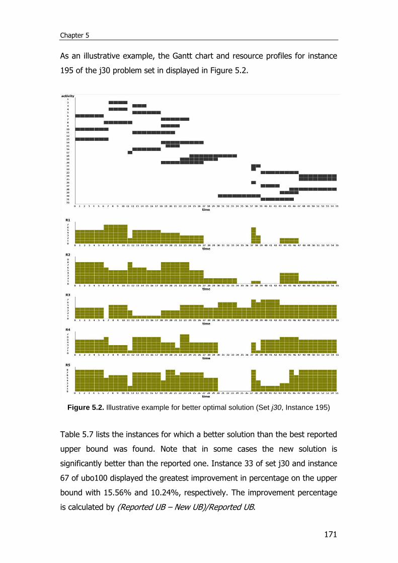
Chapter 5
171
As an illustrative example, the Gantt chart and resource profiles for instance
195 of the j30 problem set in displayed in Figure 5.2.
Figure 5.2. Illustrative example for better optimal solution (Set j30, Instance 195)
Table 5.7 lists the instances for which a better solution than the best reported
upper bound was found. Note that in some cases the new solution is
significantly better than the reported one. Instance 33 of set j30 and instance
67 of ubo100 displayed the greatest improvement in percentage on the upper
bound with 15.56% and 10.24%, respectively. The improvement percentage
is calculated by (Reported UB – New UB)/Reported UB.
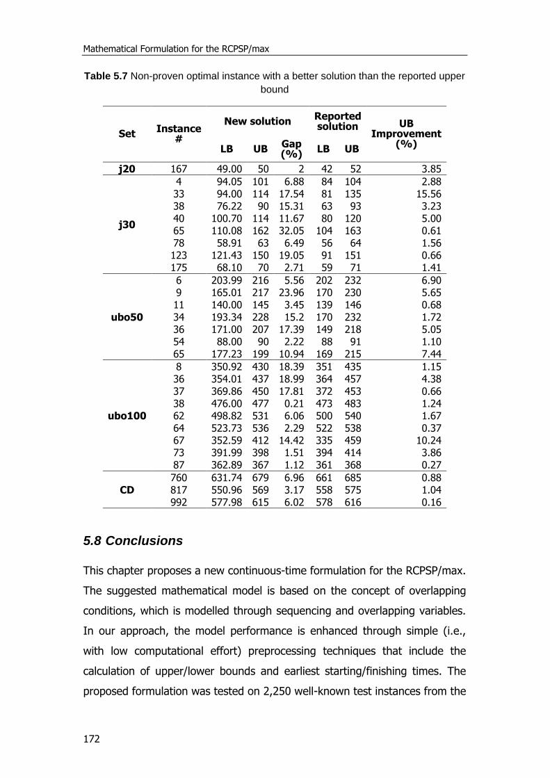
Mathematical Formulation for the RCPSP/max
172
Table 5.7 Non-proven optimal instance with a better solution than the reported upper
bound
Set Instance
#
New solution Reported solution UB
Improvement (%)
LB UB Gap (%)
LB UB
j20 167 49.00 50 2 42 52 3.85
j30
4 94.05 101 6.88 84 104 2.88 33 94.00 114 17.54 81 135 15.56 38 76.22 90 15.31 63 93 3.23 40 100.70 114 11.67 80 120 5.00 65 110.08 162 32.05 104 163 0.61 78 58.91 63 6.49 56 64 1.56 123 121.43 150 19.05 91 151 0.66 175 68.10 70 2.71 59 71 1.41
ubo50
6 203.99 216 5.56 202 232 6.90 9 165.01 217 23.96 170 230 5.65 11 140.00 145 3.45 139 146 0.68 34 193.34 228 15.2 170 232 1.72 36 171.00 207 17.39 149 218 5.05 54 88.00 90 2.22 88 91 1.10 65 177.23 199 10.94 169 215 7.44
ubo100
8 350.92 430 18.39 351 435 1.15 36 354.01 437 18.99 364 457 4.38 37 369.86 450 17.81 372 453 0.66 38 476.00 477 0.21 473 483 1.24 62 498.82 531 6.06 500 540 1.67 64 523.73 536 2.29 522 538 0.37 67 352.59 412 14.42 335 459 10.24 73 391.99 398 1.51 394 414 3.86 87 362.89 367 1.12 361 368 0.27
CD 760 631.74 679 6.96 661 685 0.88 817 550.96 569 3.17 558 575 1.04 992 577.98 615 6.02 578 616 0.16
5.8 Conclusions
This chapter proposes a new continuous-time formulation for the RCPSP/max.
The suggested mathematical model is based on the concept of overlapping
conditions, which is modelled through sequencing and overlapping variables.
In our approach, the model performance is enhanced through simple (i.e.,
with low computational effort) preprocessing techniques that include the
calculation of upper/lower bounds and earliest starting/finishing times. The
proposed formulation was tested on 2,250 well-known test instances from the

Chapter 5
173
literature, with problems sizes varying from 10 to 100 activities. The
computational results revealed a number of solutions that are better than the
ones reported in PSPLIB.
All reported infeasible instances were proven, with the exception of the CD
test set, wherein 9 out of 21 where identified. For projects with up to 30
activities, the proposed formulation solved optimally most problems. Problem
sizes of 50 activities are also dealt efficiently with a feasible solution for
91.78% and a good solution for 83.56% of the solvable instances. Finally, for
the larger sets ubo100 and CD that involve 100 activities, the reported results
were quite satisfactory for a solution method that relies on a mathematical
formulation taking into consideration the problem sizes. This declining model
performance is caused by the larger number of activities, which leads to a
polynomial increase in the number of sequencing and overlapping variables.
With the increasing computational power available, even in personal
computers, mathematical solvers are becoming capable of dealing with larger
problems than in the past. Given that the RCPSP/max is an offline problem,
we can easily accept to increase the time limit of the solver and obtain
optimal or good suboptimal solutions.
5.9 Nomenclature
Indices/Sets
1,...,1,0:, nAji activities
mk ,...,1: renewable resources
Subsets
B set of activities 2, Vji , sharing at least one renewable
resource
C transitive closure of subset L
E pairs of activities with temporal constraints
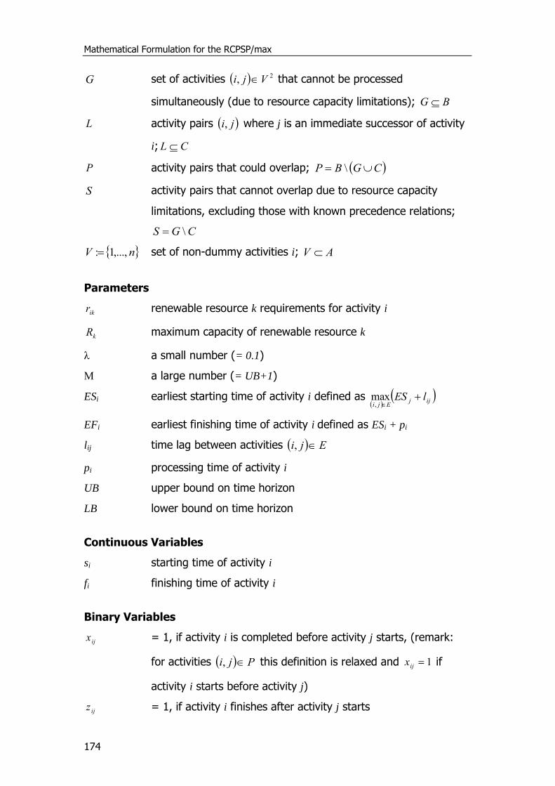
Mathematical Formulation for the RCPSP/max
174
G set of activities 2, Vji that cannot be processed
simultaneously (due to resource capacity limitations); BG
L activity pairs ji, where j is an immediate successor of activity
i; CL
P activity pairs that could overlap; CGBP \
S activity pairs that cannot overlap due to resource capacity
limitations, excluding those with known precedence relations;
CGS \
nV ,...,1: set of non-dummy activities i; AV
Parameters
ikr renewable resource k requirements for activity i
kR maximum capacity of renewable resource k
λ a small number (= 0.1)
Μ a large number (= UB+1)
ESi earliest starting time of activity i defined as
ijj
EjilES
,max
EFi earliest finishing time of activity i defined as ESi + pi
lij time lag between activities Eji ,
pi processing time of activity i
UB upper bound on time horizon
LB lower bound on time horizon
Continuous Variables
si starting time of activity i
fi finishing time of activity i
Binary Variables
ijx = 1, if activity i is completed before activity j starts, (remark:
for activities Pji , this definition is relaxed and 1ijx if
activity i starts before activity j)
ijz = 1, if activity i finishes after activity j starts
Chapter 6
175
Chapter 6
Conclusions and future work
In this chapter, we summarise the main contributions of this thesis and
discuss possible future research directions that seem promising.
6.1 Conclusions
The objective of this thesis is to establish a new representation and solution
framework for RCPSPs utilising techniques from the process scheduling area.
For this reason, a new network representation method has been developed,
based on the well-known RTN, as well as a number of mathematical
programming formulations for the RCPSP and its variants. The computational
results displayed the efficient performance of the formulations, which
outperform state-of-the-art models from the literature.
In Chapter 3, we proposed a new network representation method and
new MILP models for the RCPSP and the MRCPSP, based on the well-
known RTN process representation from the process scheduling industry.
The formulations were used to solve some project scheduling problems
from the online PSPLIB. The computational results of this initial approach,
indicated that for problems involving more than 30 activities, the proposed
MILP models cannot lead to a global optimal solution in reasonable
computational times. However the proven similarities between process
and project scheduling problems, suggested that exchanging solution
techniques between the two research fields is both possible and useful. In
summary, the main objective of this chapter, to establish a new
framework for RCPSPs utilising techniques from the process scheduling
area was achieved.
Conclusions and Future Work
176
In Chapter 4, four very efficient discrete- and continuous-time
formulations were developed, followed by a detailed comparison with four
state-of-the-art models from the literature, using 2760 RCPSPs. Also, a
number of computationally inexpensive preprocessing steps were taken to
enhance and simplify the formulations. Overall, the continuous-time
models have been found to be the best models for the problems
addressed. The detailed and comprehensive computational analysis
revealed some interesting features of the problems solved and the
mathematical models considered. In particular, it has been observed, that
problem instances with low RS values and high RF values are the most
hard to solve, according to the computational results in problem sets j30
and j60. Moreover, it seems that increasing the number of activities
directly affects negatively the computational performance of continuous-
time models since the number of sequencing binary variables is increased
dramatically, while discrete-time models are affected less due to the fact
that the number of the decisions variables principally depends on the time
points. Notice that, in contrast to continuous-time models, the
performance of discrete-time models is strongly affected (positively) from
the bounds imposed on the preprocessing phase. In addition, continuous-
time formulations featured lower Gap (%) values compared with discrete-
time models.
In Chapter 5 a new continuous-time formulation for the RCPSP/max was
proposed. The suggested mathematical model is an extension of the KKG-
CT2 model introduced in Chapter 4. The model performance was
enhanced through simple (i.e., with low computational effort)
preprocessing techniques that include the calculation of upper/lower
bounds and earliest starting/finishing times. The proposed formulation
was tested on 2,250 well-known test instances from the literature, with
problems sizes varying from 10 to 100 activities. The computational
results revealed a number of solutions that are better than the ones
reported in PSPLIB. All reported infeasible instances were proven, with the
Chapter 6
177
exception of the CD test set, wherein 9 out of 21 where identified. For
projects with up to 30 activities, the proposed formulation solved optimally
most problems. Problem sizes of 50 activities are also dealt efficiently with
a feasible solution for 91.78% and a good solution for 83.56% of the
solvable instances. Finally, for the larger sets ubo100 and CD that involve
100 activities, the reported results were quite satisfactory for a solution
method that solely relies on a mathematical formulation taking into
consideration the problem sizes.
6.2 Future Work
The results of this thesis revealed a range of issues and pointed to several
interesting directions for future work:
Further research in devising other continuous- and discrete-time
mathematical modelling approaches seems promising and highly
challenging.
Of particular interest would be the comparison of the proposed
formulations with more mathematical models from the literature
and hopefully some new ones, using the same and possibly larger
RCPSP problems (i.e. sets j90 and j120). A more extensive
computational study could provide us with further insight regarding
the performance of the available mathematical frameworks, and
could inspire the development of new modelling approaches.
Since the new continuous-time models proposed in chapters 4 and
5, have proven to be efficient for solving the RCPSP and the
RCPSP/max, a possible extension to the multi-mode RCPSP could
be considered.
The proposed models could be the core element of new
decomposition methods, such as the one proposed by Kopanos et
al. (2010), or part of hybrid methods, in an attempt to reduce the
Conclusions and Future Work
178
computational burden of the complicated problems solved and
allow us to deal with larger problems.
Given that the RCPSP is an offline problem, we can easily accept an
increase on the time limit of the solver and obtain more optimal
and/or good suboptimal solutions.
The RCPSP has a number of interesting variants, that could be
addressed. For example, since project scheduling is dynamic in
nature, the consideration of uncertainty also arises as a challenging
future research task. Three main categories of approaches can be
distinguished: proactive, reactive and stochastic.
Another interesting extension, is the Resource Levelling Problem
(RLP), which arises whenever it is expedient to reduce the
fluctuations in patterns of resource utilizations over time, while
maintaining compliance with a prescribed project completion time.
In particular, in cases where even slight variations in resource
needs represent financial burden or heightened risks of accidents, a
resource levelling approach helps to schedule the project activities
such that the resource utilization will be as smooth as possible over
the entire planning horizon. Under resource levelling, no resource
limits are typically imposed. Therefore, only the time lags between
individual activities form the project constraints.
Finally, if we reverse the scope of this thesis, we could transfuse
solution techniques and concepts from project scheduling literature
to process scheduling.
Hopefully, this work will motivate further research in developing better and/or
improved modelling frameworks for the standard RCPSP.
Publications
179
Publications
This is a list of the works carried out so far within the scope of interest of this
thesis, in reversed chronological order. The list has been divided in papers
submitted to international refereed journals and published in conference
proceedings:
Scientific Journals
Manuscript published
[1] Kyriakidis, T.S., Kopanos, G.M., Georgiadis, M.C., 2012. MILP
formulations for single- and multi-mode resource-constrained project
scheduling problems, Computers & Chemical Engineering 36, 369–385.
Manuscripts submitted
[1] Kyriakidis, T.S., Kopanos, G.M., Georgiadis, M.C., 2012. Mathematical
Formulation for Resource-Constrained Project Scheduling Problems with
Generalized Precedence Relations, OR Spectrum (September 2012,
under review).
[2] Kopanos, G.M., Kyriakidis, T.S., Georgiadis, M.C., 2012. New
Continuous-time and Discrete-time Mathematical Formulations for
Resource-constrained Project Scheduling Problems, European Journal of
Operational Research (January 2012, 1st revision completed).
Conference Proceeding Articles
The work realised in this thesis has been also presented and published to
different international specialised conferences. The RCPSP/max formulation
proposed in Chapter 5, is very recent and has not been submitted to any
conferences yet. A list of publications in conferences proceedings follows:
Publications
180
[1] Kyriakidis, T.S., Georgiadis, M.C., Solving resource-constrained project
scheduling problems with new mathematical programming formulations,
25th European Conference on Operational Research (EURO 2012), 8-11
July 2012, Vilnius, Lithuania.
[2] Kopanos, G.M., Kyriakidis, T.S., Georgiadis, M.C., New Mathematical
Programming Formulations for Resource-Constrained Project Scheduling
Problems, 9th International Conference on Computational Management
Science (CMS 2012), 18-20 April 2012, London, United Kingdom.
[3] Kyriakidis, T.S., Kopanos, G.M., Georgiadis, M.C., MILP Formulation for
Resource-Constrained Project Scheduling Problems, 21st European
Symposium on Computer Aided Process Engineering (ESCAPE-21), 29
May-01 June 2011, Porto Carras, Greece, In Proceedings: 880-884.
References
181
References
Ahuja, R., Magnanti, T., Orlin, J., 1993. Network Flows. Prentice Hall,
Englewood Cliffs.
Achuthan, N.R., Hardjawidjaja, A., 2005. Project scheduling under time
dependent costs - A branch and bound algorithm. Annals of Operations
Research 108 (1-4), 55-74.
Agrawal, M.K., Elmaghraby, S.E., Herroelen, W.S., 1996. DAGEN: A generator
of testsets for project activity nets. European Journal of Operational Research
90. 376–82.
Alcaraz, J., Maroto, C., Ruiz, R., 2004. Improving the performance of genetic
algorithms for the RCPS problem. Proceedings of the Ninth International
Workshop on Project Management and Scheduling, Nancy, 40–3.
Al-Fawzana, M.A., Haouari, M., 2005. A bi-objective model for robust
resource-constrained project scheduling. International Journal of Production
Economics 96, 175–87.
Alcaraz, J., Maroto, C., Ruiz, R., 2003. Solving the multi-mode resource-
constrained project scheduling problem with genetic algorithms. Journal of
the Operational Research Society 54 (6), 614–26.
Alvarez-Valdes, R., Tamarit, J.M., 1993. The project scheduling polyhedron:
Dimension, facets and lifting theorems. European Journal of Operational
Research 67 (2), 204-20.
Alvarez-Valdes, R., Tamarit, J.M., 1989. Heuristic algorithms for resource-
constrained project scheduling: a review and an empirical analysis. In:
Slowinski, R., Węglarz, J., editors. Advances in project scheduling, p. 113–34.
Elsevier, Amsterdam.
References
182
Artigues, C., Michelon, P., Reusser, S., 2003. Insertion techniques for static
and dynamic resource-constrained project scheduling. European Journal of
Operational Research 149 (2), 249-67.
Ballestin, F., Barrios, A., Valls, V., 2011. An evolutionary algorithm for the
resource-constrained project scheduling problem with minimum and
maximum time lags. Journal of Scheduling 14, 391-406.
Bard, J.F., Kontoravdis, G., Yu, G., 2002. A branch-and-cut procedure for the
vehicle routing problem with time windows. Transportation Science 36, 250–
69.
Bartusch, M., Möhring, R.H., Radermacher, F.J., 1988. Scheduling project
networks with resource constraints and time windows. Annals of Operations
Research 16, 201–40.
Bianco, L., Caramia, M., 2012a. A new formulation for the project scheduling
problem under limited resources. Flexible Services and Manufacturing Journal
2012. published online.
Bianco, L., Caramia, M., 2012b. An exact algorithm to minimize the makespan
in project scheduling with scarce resources and generalized precedence
relations. European Journal of Operational Research 219, 73-85.
Blazewicz, J., Lenstra, J. Κ., Rinnooy Kan, A. H. G., 1983. Scheduling subject
to resource constraints: classification and complexity. Discrete Applied
Mathematics 5 (1), 11-24.
Bomsdorf, F., Derigs, U., 2008. A model, heuristic procedure and decision
support system for solving the movie shoot scheduling problem. OR Spectrum
30 (4), 751–72.
Böttcher, J., Drexl, A., Kolisch, R., 1996. A Branch-and-Bound Procedure for
Project Scheduling with Partially Renewable Resource Constraints.
Proceedings of the Fifth Workshop on Project Management and Scheduling,
Poznan, April 11-13, 48-51.
References
183
Böttcher, J., Drexl, A., Kolisch, R., Salewski, F., 1999. Project scheduling
under partially renewable resource constraints. Management Science 45(4),
543–59.
Browning, T.R., Yassine, A.A., 2007. A Random Generator of Resource-
constrained Multi-project Scheduling Problems, Technical Report, Texas
Christian University, M.J. Neeley School of Business.
Brucker, P., Drexl, A., Mohring, R., Neumann, Κ., Pesch, E., 1999. Resource-
constrained project scheduling: Notation, classification, models, and methods.
European Journal of Operational Research 112 (1), 3-41.
Castillo, E., Conejo, A.J., Pedregal, P., García, R., Alguaci, N., 2001. Building
and Solving Mathematical Programming Models in Engineering and Science.
New York, USA: John Wiley & Sons.
Castro, P., Barbosa-Póvoa, A.P., Matos, H.A., 2001. An Improved Continuous-
Time Formulation for the Short-term Scheduling of Multipurpose Batch Plants.
Industrial and Engineering Chemistry Research 40, 2059-68.
Castro, P.M., Barbosa-Póvoa, A.P., Matos, H.A., Novais, A.Q., 2004. Simple
Continuous-Time Formulation for Short-Term Scheduling of Batch and
Continuous Processes. Industrial and Engineering Chemistry Research 43,
105-18.
Cesta, A., Oddi, A., Smith, S., 2002. A constraint based method for project
scheduling with time windows. Journal of Heuristics 8(1), 109-36.
Christofides, N., Alvarez-Valdes, R., Tamarit, J. M., 1987. Project scheduling
with resource constraints: a branch-and-bound approach. European Journal
of Operational Research 29 (3), 262-73.
Cicirello, V.A., Smith, S.F., 2004. Heuristic selection for stochastic search
optimization: Modeling solution quality by extreme value theory. In:
Proceedings of the 10th International Conference on Principles and Practice
of Constraint Programming. CP 2004, Toronto, Canada, 197-211.
References
184
Coelho, J., Vanhoucke, M., 2011. Multi-mode resource-constrained project
scheduling using RCPSP and SAT solvers. European Journal of Operational
Research 213, 73–82.
Colvin, M., Maravelias, C.T., 2008. A stochastic programming approach for
clinical trial planning in new drug development. Computers and Chemical
Engineering 32, 2626-42.
Colvin, M., Maravelias, C.T., 2009. Scheduling of testing tasks and resource
planning in new product development using stochastic programming.
Computers and Chemical Engineering 33 (5), 964-76.
Colvin, M., Maravelias, C.T., 2010. Modeling methods and a branch and cut
algorithm for pharmaceutical clinical trial planning using stochastic
programming. European Journal of Operational Research 203, 205-15.
De Reyck, B., Herroelen, W.S., 1998. A branch-and-bound procedure for the
resource-constrained project scheduling problem with generalized precedence
relations. European Journal of Operational Research 111 (1), 152–74.
Debels, D., De Reyck, B., Leus, R., Vanhoucke, M., 2006. A hybrid scatter
search/Electromagnetism meta-heuristic for project scheduling. European
Journal of Operational Research 169 (2), 638-53.
Debels, D., Vanhoucke, M., 2008. A Decomposition-Based Genetic Algorithm
for the Resource-Constrained Project-Scheduling Problem. Operations
Research 55 (3), 457–69.
Demassey, S., Artigues, C., Michelon, P., 2005. Constraint propagation based
cutting planes: an application to the resource-constrained project scheduling
problem. INFORMS Journal on Computing 17 (1), 52-65.
Demeulemeester, E.L., 1995. Minimizing Resource-Availability Costs in Time-
Limited Project Networks, Management Science 41, 1590-8.
References
185
Demeulemeester, E.L., Herroelen, W.S., 2002. Project Scheduling: A Research
Handbook. Kluwer Academic Publishers, Boston.
Demeulemeester, E.L., Herroelen, W.S., 1997a. New benchmark results for
the resource-constrained project scheduling problem. Management Science
43 (11), 1485–92.
Demeulemeester, E.L., Herroelen, W.S., 1997b. A branch-and-bound
procedure for the generalized resource-constrained project scheduling
problem. Operations Research 45, 201–12.
Demeulemeester, E.L., Herroelen, W.S., 1992. A branch-and-bound
procedure for the multiple resource-constrained project scheduling problem.
Management Science 38 (12), 1803–18.
Demeulemeester, E.L., Vanhoucke, M., Herroelen, W.S., 2003. RanGen: A
random network generator for activity-on-the-node networks. Journal of
Scheduling 6 (1), 17-38.
Dorndorf, U., Pesch, E., Phan-Huy, T., 2000. A time-oriented branch-and-
bound algorithm for resource-constrained project scheduling with generalised
precedence constraints. Management Science 46, 1365-84.
Drexl, A., 1997. Local Search Methods for Project Scheduling under Partially
Renewable Resource Constraints, Paper presented at the INFORMS San Diego
Spring Meeting, May 4-7, 1997.
Eisner, H., 1962. A generalized network approach to the planning and
scheduling of a research project. Operations Research 10 (1), 115-125.
Elmaghraby, S.E., Kamburowski J., 1992. The Analysis of Activity Networks
under Generalized Precedence Relations (GPRs). Management Science 38 (9),
1245-63.
Elmaghraby, S.E., 1977. Activity Networks – Project Planning and Control by
Network Models, John Wiley & Sons Inc., New York.
References
186
Ferris, M., 1999. MATLAB and GAMS: Interfacing optimization and
visualization software. Technical report, University of Wisconsin.
Fest, A., Möhring, R.H., Stork, F., Uetz, M., 1998. Resource-constrained
project scheduling with time windows: a branching scheme based on dynamic
release dates. Technical Report 596, Technical University of Berlin. (Revised
in 1999).
Franck, B., Schwindt, C., 1995. Different Resource-Constrained Project
Scheduling Models with Minimal and Maximal Time-Lags, Technical Report
WIOR-450, Universität Karlsruhe, Germany.
Franck, B., Neumann, K., 1998. Resource Constrained Project Scheduling
Problems with Time Windows - Structural Questions and Priority-Rule
Methods. Technical Report WIOR-492, University of Karlsruhe, Germany.
Franck, B., Neumann, K., Schwindt, C., 2001. Truncated branch and bound,
schedule construction, and schedule improvement procedures for resource
constrained project scheduling. OR Spectrum 23, 297–324.
GAMS Development Corporation (2007). GAMS/Cplex 11 User Notes.
Glover, F., 1975. Improved linear integer programming formulations of
nonlinear integer problems. Management Science 22 (4), 455–60.
Gomory, R.E., 1960. An algorithm for the mixed integer problem. Technical
Report RM-2597, The Rand Corporation.
Gomory, R.E., 1958. Outline of an Algorithm for Integer Solutions to Linear
Programs. Bulletin Of the American Mathematical Society 64, 275–8.
Graham, R.L., Lawler, E.L., Lenstra, J.K., Rinnooy Kan, A.H.G., 1979.
Optimisation and approximation in deterministic sequencing and scheduling:
A survey. Annals of Discrete Mathematics 5 (2), 287-326.
References
187
Hartmann, S., 2002. A self-adapting genetic algorithm for project scheduling
under resource constraints. Naval Research Logistics 49, 433–48.
Hartmann, S., 2001. Project scheduling with multiple modes: a genetic
algorithm. Annals of Operations Research 102 (1–4), 111–35.
Hartmann, S., Briskorn, D., 2010. A survey of variants and extensions of the
resource-constrained project scheduling problem. European Journal of
Operational Research 207, 1-14.
Hartmann, S., Drexl, A., 1998. Project scheduling with multiple modes: a
comparison of exact algorithms. Networks 32, 283–97.
Hartmann, S., Kolisch, R., 2000. Experimental evaluation of state-of-the-art
heuristics for the resource-constrained project scheduling problem. European
Journal of Operational Research 127 (2), 394-407.
Herroelen, W.S., 2005. Project Scheduling - Theory and Practice. Production
and Operations Management 14 (4), 413-32.
Herroelen, W.S., De Reyck, B., Demeulemeester, E..L. 1998. A Classification
Scheme for Project Scheduling, In Węglarz, J. (Ed.), Handbook of Recent
Advances in Project Scheduling, Kluwer Academic Publishers, 1-26.
International Organization for Standardization, 2003. ISO 10006: Guideline
for Quality in Project Management. ISO Press, Geneva.
Jain, V., Grossmann, I.E., 1999. Resource-constrained scheduling of tests in
new product development. Industrial and Engineering Chemistry Research 38,
3013-26.
Jarboui, B., Damak, N., Siarry, P., Rebai, A., 2008. A combinatorial particle
swarm optimization for solving multi-mode resource-constrained project
scheduling problems. Applied Mathematics and Computation 195, 299–308.
References
188
Kaplan, L.A., 1988. Resource-constrained project scheduling with preemption
of jobs. Ph.D. thesis, University of Michigan.
Karmarkar, N., 1984. A New Polynomial-Time Algorithm for Linear
Programming. Combinatorica 4, 373-95.
Kelley, Jr, J. E., Walker, M. R., 1959. Critical-path planning and scheduling.
In: Papers presented at the December 1-3, 1959, eastern joint IRE-AIEE-ACM
computer conference. IRE-AIEE-ACM ’59 (Eastern). ACM, New York, NY, USA,
pp. 160-73.
Kimms, A., 1998. Optimization Guided Lower and Upper Bounds for the
Resource Investment Problem, Research Report 481, Universitat Kiel,
Germany.
Klein, R., 2000. Scheduling of resource-constrained projects. Kluwer
Academic Publishers, Boston.
Kochetov, Y., Stolyar, A., 2003. Evolutionary local search with variable
neighborhood for the resource constrained project scheduling problem.
Proceedings of the 3rd International Workshop of Computer Science and
Information Technologies, Russia.
Kolisch, R., 2000. Integrated scheduling, assembly area- and part-assignment
for large-scale, make-to-order assemblies. International Journal of Production
Economics 64 (1-3), 127-42.
Kolisch, R., 1996a. Serial and parallel resource-constrained project scheduling
methods revisited: theory and computation. European Journal of Operational
Research 90 (2), 320-33.
Kolisch, R., 1996b. Efficient Priority Rules for the Resource-Constrained
Project Scheduling Problem. Journal of Operations Management 14, 179-192.
Kolisch, R., 1995. Project Scheduling under Resource Constraints – Efficient
Heuristics for Several Problem Classes, Physica-Verlag, Heidelberg.
References
189
Kolisch, R., Hartmann, S., 2006. Experimental investigation of heuristics for
resource-constrained project scheduling: An update. European Journal of
Operational Research 174 (1), 23-37.
Kolisch, R., Padman, R., 2001. An integrated survey of deterministic project
scheduling. Omega 29, 249-72.
Kolisch, R., Sprecher, A., 1996. PSPLIB - a project scheduling problem library.
European Journal of Operational Research 96 (1), 205-16.
Kolisch, R., Schwindt, C., Sprecher A., 1998. Benchmark Instances for Project
Scheduling Problems. In J. Węglarz, editor, Handbook on Recent Advances in
Project Scheduling. Kluwer.
Kolisch, R., Sprecher, A., Drexl, A., 1995. Characterization and generation of
a general class of resource-constrained project scheduling problems.
Management Science 41 (10), 1693-703.
Kone, O., Artigues, C., Lopez, P., Mongeau, M., 2011. Event-based MILP
models for resource-constrained project scheduling problems. Computers &
Operations Research 38 (1), 3-13.
Kopanos, G.M., Mendez, C.A., Puigjaner, L., 2010. MIP-based decomposition
strategies for large-scale scheduling problems in multiproduct multistage
batch plants: A benchmark scheduling problem of the pharmaceutical
industry. European Journal of Operational Research 207 (2), 644-55.
Kyriakidis, T.S., Kopanos, G.M., Georgiadis, M.C., 2012a. Solving Resource-
Constrained Project Scheduling Problems through new Mathematical
Programming Formulations. Proceedings of the European Conference on
Operational Research (EURO 2012), Vilnius, Lithuania, 240.
Kyriakidis, T. S., Kopanos, G. M., Georgiadis, M. C., 2012b. MILP formulations
for single- and multi-mode resource-constrained project scheduling problems.
Computers & Chemical Engineering 36, 369-85.
References
190
Lancaster, J., Ozbayrak, M., 2007. Evolutionary algorithms applied to project
scheduling problems - a survey of the state-of-the-art. International Journal
of Production Research 45 (2), 425–50.
Land, A.H., Doig, A. G., 1960. An automatic method for solving discrete
programming problems. Econometrica 28, 497–520.
Levis, A.A., Papageorgiou, L.G., 2004. A hierarchical solution approach for
multi-site capacity planning under uncertainty in the pharmaceutical industry.
Computers and Chemical Engineering 28, 707-25.
Malcolm, D.G., Roseboom, J. H., Clark, C.E, Fazar W., 1959. Application of a
technique for research and development program evaluation. Operations
Research 7(5), 646-69.
Maravelias, C.T., Grossmann, I.E., 2004. Optimal resource investment and
scheduling of tests for new product development. Computers and Chemical
Engineering 28, 1021-38.
Marchetti, P.A., Cerda, J., 2009. A general resource-constrained scheduling
framework for multistage batch facilities with sequence-dependent
changeovers. Computers & Chemical Engineering 33 (4), 871-86.
Mingozzi, A., Maniezzo, V., Ricciardelli, S., Bianco, L., 1998. An exact
algorithm for the resource-constrained project scheduling problem based on a
new mathematical formulation. Management Science 44 (5), 715-29.
Minieka, E., 1978. Optimization algorithms for Networks and Graphs. Marcel
Dekker Inc., New York.
Mitchell, J.E., 2001. Branch-and-cut algorithms for integer programming. In
the Encyclopedia of Optimization, Volume II, pages 519-25, Kluwer Academic
Publishers.
References
191
Möhring, R.H., 1984. Minimizing Costs of Resource Requirements in Project
Networks Subject to a Fixed Completion Time, Operations Research 32, 89-
120.
Möhring, R.H., Schulz, A., Stork, F., Uetz, M., 2003. Solving project
scheduling problems by minimum cut computations. Management Science 49
(3), 330-50.
Nabrzyski, J., Węglarz, J., 1994. A Knowledge-Based Multiobjective Project
Scheduling System. Revue des Systemes de Decision, 3, 185-200.
Nemhauser, G. L., Wolsey, L. A., 1999. Integer and Combinatorial
Optimization. Discrete Mathematics and Optimization. Wiley - Interscience,
New York.
Neumann, K., Schwindt, C., 1995. Projects with Minimal and Maximal Time
Lags: Construction of Activity-on-Node Networks and Applications. Technical
Report WIOR-447. Institüt fur Wirtschaftstheorie und Operations Research,
University of Karlsruhe.
Neumann, K., Schwindt, C., Zimmermann, J., 2003. Project Scheduling with
Time Windows and Scarce Resources. Springer, Berlin.
Neumann, K., Schwindt, C., Zimmermann, J., 2002. Project Scheduling with
Time Windows and Scarce Resources: Temporal and Resource-Constrained
Project Scheduling with Regular and Nonregular Objective Functions.
Springer, Berlin.
Neumann, K., Zimmermann, J., 2000. Procedures for resource leveling and
net present value problems in project scheduling with general temporal and
resource constraints. European Journal of Operational Research 127, 425-43.
Neumann, K., Zimmermann, J., 1999. Heuristic methods for resource-
constrained project scheduling with regular and nonregular objective
functions and schedule-dependent time windows. In: Węglarz J (ed) Project
References
192
Scheduling: Recent Models, Algorithms, and Applications. Kluwer Academic
Publishers, Boston, pp 261-87.
Pantelides, C.C., 1994. Unified frameworks for optimal process planning and
scheduling. In: Proceedings of the Second Conference on Foundations of
Computer-Aided Process Operations. CACHE, pp. 253-74.
Papageorgiou, L.G., Rotstein, G.E., Shah, N., 2001. Strategic supply chain
optimization for the pharmaceutical industries. Industrial and Engineering
Chemistry Research 40, 275-86.
Paraskevopoulos, D.C., Tarantilis, C.D., Ioannou, G., 2012. Solving project
scheduling problems with resource constraints via an event list-based
evolutionary algorithm. Expert Systems with Applications 39, 3983–94.
Patterson, J.H., 1976. Project scheduling: The effects of problem structure on
heuristic scheduling. Naval Research Logistics 23 (1), 95-123.
Pinto, J.M., Grossmann, I.E., 1995. A continuous time MILP model for short
term scheduling of batch plants with pre-ordering constraints. Industrial &
Engineering Chemistry Research 34 (9), 3037–51.
Pritsker, A.A.B., Watters, L.J., Wolfe, P.M., 1969. Multiproject scheduling with
limited resources: a zero-one programming approach. Management Science
16 (1), 93-108.
Rieck, J., Zimmermann, J., Gather, T., 2012. Mixed-integer linear
programming for resource leveling problems. European Journal Operational
Research 221, 27-37.
Rosenthal, R.E., 2012. GAMS - A User’s Guide. GAMS Development
Corporation, Washington, Washington, DC, USA.
Russell, J.R.M., 1970. Cash Cows in networks Management Science 16 (5),
357-73.
References
193
Sabzehparvar, M., Seyed-Hosseini, S.M., 2008. A mathematical model for the
multi-mode resource-constrained project scheduling problem with mode
dependent time lags. Journal of Supercomputing 44 (3), 257-73.
Salewski, F., Schirmer, A., Drexl, A., 1997. Project scheduling under resource
and mode identity constraints: Model, complexity, methods, and application.
European Journal Operational Research 102, 88-110.
Schirmer, A., Drexl, A., 1996. Partially Renewable Resources – A
Generalisation of Resource-Constrained Project Scheduling, Paper presented
at the IFORS Triennial Meeting, Vancouver, B.C., July 8-12.
Schilling, G., Pantelides, C.C., 1996. A simple continuous-time process
scheduling formulation and a novel solution algorithm. Computers and
Chemical Engineering 20, S1221-S1226.
Schmidt, C.W., Grossmann, I.E., 1996. Optimization models for the
scheduling of testing tasks in new product development. Industrial and
Engineering Chemistry Research 35, 3498-510.
Schwindt, C., 1996. Generation of resource-constrained scheduling problems
with minimal and maximal time Lags. Technical Report WIOR-489. Institüt fur
Wirtschaftstheorie und Operations Research, University Karlsruhe, Germany.
Schwindt, C., 1998a. A branch-and-bound algorithm for the resource-
constrained project duration problem subject to minimum and maximum time
lags. Technical Report WIOR-544. Institüt fur Wirtschaftstheorie und
Operations Research, University of Karlsruhe, Germany.
Schwindt, C., 1998b. Verfahren zur Lösung des ressourcenbeschränkten
Projektdauerminimierungs problems mit planungsabhängigen Zeitfenstern.
Shaker Verlag, Aachen, Germany.
Slowinski, R., 1980. Two approaches to problems of resource allocation
among project activities - a comparative study. The Journal of the
Operational Research Society 31 (8), 711-23.
References
194
Smith, T., 2004. Windows-based project scheduling algorithms. Dissertation,
University of Oregon.
Sprecher, A., Hartmann, S., Drexl, A., 1997. An exact algorithm for project
scheduling with multiple modes. OR Spektrum 19 (3), 195–203.
Stinson, J.P., Davis, E.W., Khumawala, B.M., 1978. Multiple resource-
constrained scheduling using branch and bound. AIIE Transactions 10, 252–
9.
Talbot, F.B., 1982. Resource-constrained project scheduling with time-
resource tradeoffs: the nonpreemptive case. Management Science 28 (10),
1197-1210.
Tavares, L. V., Ferreira, J. A., Coelho, J. S., 1999. The risk of delay of a
project in terms of the morphology of its network. European Journal of
Operational Research 119 (2), 510-37.
The Mathworks, Inc., 1998. MATLAB: The Language of Technical Computing:
MATLAB Notebook User’s Guide. Natick, MA, USA: The Mathworks Inc.
Valls, V., Ballestin, F., Quintanilla, M.S., 2003. A hybrid genetic algorithm for
the RCPSP. Technical report, Department of Statistics and Operations
Research, University of Valencia.
Valls, V., Ballestin, F., Quintanilla, M.S., 2005. Justification and RCPSP: A
technique that pays. European Journal of Operational Research 165, 375-86.
Van Peteghem, V., Vanhoucke, M., 2010. A genetic algorithm for the
preemptive and non-preemptive multi-mode resource-constrained project
scheduling problem. European Journal of Operational Research 201, 409–18.
Vanhoucke, M., Coelho, J., Debels, D., Maenhout, B., Tavares, L. V., 2008. An
evaluation of the adequacy of project network generators with systematically
sampled networks. European Journal of Operational Research 187 (2), 511-
24.
References
195
Węglarz, J., 1979. Project scheduling with discrete and continuous resources.
IEEE Transactions on Systems, Man and Cybernetics 9 (10), 644–50.
Węglarz, J., Jozefowska, J., Mika, M., Waligora, G., 2011. Project scheduling
with finite or infinite number of activity processing modes - A survey.
European Journal of Operational Research 208, 177–205.
Yang, X.S., 2008. Introduction to Computational Mathematics. World
Scientific Publishing, Singapore.
Zapata, J.C., Hodge, B.M., Reklaitis, G.V., 2008. The Multimode Resource
Constrained Multiproject Scheduling Problem: Alternative Formulations.
AICHE 54(8), 2101-19.
Zhu, G., Bard, J.F., Ju, G., 2006. A branch-and-cut procedure for the
multimode resource-constrained project-scheduling problem. INFORMS
Journal on Computing 18 (3), 377-90.
Zimmermann, J., 1997. Heuristics for Resource-Leveling Problems in Project
Scheduling with Minimum and Maximum Time-Lags, Technical Report WIOR-
491, Universität Karlsruhe, Germany.