Optimizing Deeper Transformers on Small Datasets

Peng Xu1, Dhruv Kumar∗1,2, Wei Yang1, Wenjie Zi1, Keyi Tang1, Chenyang Huang∗1,5,Jackie Chi Kit Cheung1,3,4, Simon J.D. Prince1, Yanshuai Cao1

1Borealis AI 2University of Waterloo3McGill University 4Canada CIFAR Chair, Mila 5University of Alberta

{peng.z.xu, wei.yang, wenjie.zi, keyi.tang, simon.prince, yanshuai.cao}@borealisai.com

dhruv.kumar@uwaterloo.ca, chuang8@ualberta.ca, jcheung@cs.mcgill.ca

Abstract

It is a common belief that training deep trans-formers from scratch requires large datasets.Consequently, for small datasets, people usu-ally use shallow and simple additional lay-ers on top of pre-trained models during fine-tuning. This work shows that this does not al-ways need to be the case: with proper initial-ization and optimization, the benefits of verydeep transformers can carry over to challeng-ing tasks with small datasets, including Text-to-SQL semantic parsing and logical readingcomprehension. In particular, we success-fully train 48 layers of transformers, com-prising 24 fine-tuned layers from pre-trainedRoBERTa and 24 relation-aware layers trainedfrom scratch. With fewer training steps andno task-specific pre-training, we obtain thestate-of-the-art performance on the challeng-ing cross-domain Text-to-SQL parsing bench-mark Spider1. We achieve this by derivinga novel Data-dependent Transformer Fixed-update initialization scheme (DT-Fixup), in-spired by the prior T-Fixup work (Huang et al.,2020). Further error analysis shows that in-creasing depth can help improve generaliza-tion on small datasets for hard cases that re-quire reasoning and structural understanding.

1 Introduction

In recent years, large-scale pre-trained languagemodels (Radford et al., 2019; Devlin et al.,2018; Liu et al., 2019b) trained with transform-ers (Vaswani et al., 2017) have become standardbuilding blocks of modern NLP systems to helpimprove generalization when task-specific annota-tions are limited. In practice, it has been foundthat deeper transformers generally yield better re-sults with sufficient training data (Lan et al., 2019),

∗Work done while the author was an intern in Borealis AI.1The code to reproduce our results can be found in:

https://github.com/BorealisAI/DT-Fixup

especially on tasks involving reasoning and struc-tural understanding. This suggests that additionaltransformer layers should be employed in conjunc-tion with pre-trained models, instead of simple andshallow neural components, such as a classifierhead, currently used by models of many NLP tasks.However, the common belief in the literature is thattraining deep transformers from scratch requireslarge datasets, and few attempts have been made onsmall datasets, to the best of our knowledge. Oneimplication is that although extra transformer lay-ers on top of pre-trained models should help withmore challenging problems in principle, it doesnot work in practice due to limited training data.We show that after resolving several optimizationissues with the method proposed in this work, itis possible to train very deep transformers withimproved generalization even on small datasets.

One advantage of pre-trained models is the re-duced computational resources needed when fine-tuning on small datasets. For instance, it allowspractitioners to finetune on a single GPU and obtainstrong performance on a downstream task. How-ever, the large size of pre-trained models limits thebatch size that can be used in training new trans-former layers on a small computational budget. De-spite their broad applications, training transformermodels is known to be difficult (Popel and Bojar,2018). The standard transformer training approachleverages learning rate warm-up, layer normaliza-tion (Ba et al., 2016) and a large batch size, andmodels typically fail to learn when missing anyone of these components. The restricted batch sizeaggravates the training difficulties. Even if a largebatch size can be feasibly employed, poorer gener-alization results are often observed (Keskar et al.,2016), especially when the dataset size is only sev-eral times larger than the batch size. Furthermore,many recent works noticed a performance gap inthis training approach due to layer normalization

arX

iv:2

012.

1535

5v4

[cs

.CL

] 3

1 M

ay 2

021

(Xu et al., 2019; Nguyen and Salazar, 2019; Zhanget al., 2019a; Wang et al., 2019b; Liu et al., 2020;Huang et al., 2020).

Inspired by the recent T-Fixup by Huang et al.(2020), which eliminates the need for learning ratewarm-up and layer normalization to train vanillatransformers, we derive a data-dependent initial-ization strategy by applying different analyses toaddress several key limitations of T-Fixup. Wecall our method the Data-dependent TransformerFixed-update initialization scheme, DT-Fixup. Inthe mixed setup of additional yet-to-be-trainedtransformers on top of pre-trained models, DT-Fixup enables the training of significantly deepertransformers, and is generally applicable to differ-ent neural architectures. Our derivation also ex-tends beyond vanilla transformers to transformerswith relational encodings (Shaw et al., 2018), al-lowing us to apply the results to one variant calledrelation-aware transformer (Wang et al., 2019a).By applying DT-Fixup on different tasks, we showthat the impression that deep transformers do notwork on small datasets stems from the optimizationprocedure rather than the architecture. With properinitialization and optimization, training extra trans-former layers is shown to facilitate the learning ofcomplex relations and structures in the data.

We verify the effectiveness of DT-Fixup on Spi-der (Yu et al., 2018), a complex and cross-domainText-to-SQL semantic parsing benchmark, andReColr (Yu et al., 2020b), a reading comprehensiondataset requiring logical reasoning. While Text-to-SQL semantic parsing is inherently different fromreading comprehension, they share similar charac-teristics which require certain levels of reasoningand structural understanding ability. Meanwhile,the sizes of both datasets are less than 10k trainingsamples, which is tiny by deep learning standardsand renders large-batch training undesirable due topoor generalization2.

On both datasets, DT-Fixup consistently out-performs the standard approach with better gen-eralization and allows the training of significantlydeeper transformer models. For Spider, we suc-cessfully apply DT-Fixup to train a Text-to-SQLparser containing 48 transformer layers, with 24relation-aware layers trained from scratch on topof 24 pre-trained layers from pre-trained RoBERTa

2For a comparison, T-Fixup applies batch sizes of morethan 1k on machine translation to stabilize the training, whichwould hurt the generalization significantly on our datasetswhose sizes are less than 10k.

(Liu et al., 2019b). Our parser achieves 70.9% ex-act match accuracy on the Spider test set, whichis the state of the art at the time of writing. At thesame time, it requires less training steps and notask-specific pre-training as compared to the priorart (Yu et al., 2020a). For ReClor, we rank thesecond on the public leaderboard by simply adding4 transformer layers on top of RoBERTa. Furthererror analysis shows that the performance improve-ments by increasing the depth mainly come frombetter generalization on the harder cases requiringreasoning and structural understanding. Even thefailed predictions from the deep models are morereasonable than from the shallow ones.

2 Background

In this section, we present the necessary back-ground by first introducing the relation-aware trans-former layer, which outperforms the vanilla trans-former layer with limited data by injecting addi-tional inductive bias (Wang et al., 2019a). Then,we introduce the T-Fixup technique (Huang et al.,2020) for optimizing deeper vanilla transformersand discuss why it does not directly apply in themixed transformer optimization setup.

2.1 Relative Position and RelationalEncodings in Transformers

Consider a set of inputs X = [xxx1, . . . ,xxxn] wherexxxi ∈ Rdx . A transformer, introduced by Vaswaniet al. (2017), is a stack of blocks, with each blockconsisting of a multi-head self-attention layer, layernormalizations, a multi-layer perceptron and skipconnections. Each block (with one head in self-attention for notational simplicity) transforms eachxxxi into yyyi ∈ Rdx as follows:

αij = softmax(xxxiqqq(xxxjkkk)>

/√dz

)(1)

zzzi =∑n

j=1αijxxxjvvv; (2)

yyyi = LayerNorm(xxxi + zzziwww>) (3)

yyyi = LayerNorm(yyyi + MLP(yyyi)) (4)

where the softmax operation is applied across theindex j, MLP is a two-layer perceptron, Layer-Norm is a layer normalization (Ba et al., 2016)layer, and qqq,kkk,vvv ∈ Rdx×dz ,www ∈ Rdx×dz .

In order to bias the transformer toward somepre-existing relational features between the inputs,Shaw et al. (2018) described a way to represent rel-ative position information in a self-attention layer

by changing Equation 1-2 as follows:

αij = softmax

(xxxiqqq(xxxjkkk + rrrkij)

>√dz

)zzzi =

∑nj=1αij(xxxjvvv + rrrvij)

(5)

Here the rrrij ∈ Rdz terms encode the known re-lationship between two elements xxxi and xxxj in theinput. Wang et al. (2019a) adapted this frameworkto effectively encode the schema information usingrrrij’s for Text-to-SQL parsers, and called it relation-aware transformer (RAT).

2.2 T-Fixup and its LimitationsHuang et al. (2020) found that the requirementfor the warmup during the early stage training ofthe transformers comes from a combined effectof high variance in the Adam optimizer and back-propagation through layer normalization. Bound-ing the gradient updates would reduce the varianceand make training stable, which can be achievedby appropriately initializing the model weights.

They derived a weight initialization schemecalled T-Fixup for the vanilla transformer that fullyeliminates the need for layer normalization andlearning rate warmup, and stabilizes the trainingto avoid harmful plateaus of poor generalization.T-Fixup requires the inputs xxx to be Gaussian ran-domly initialized embeddings with variance d−

12

where d is the embedding dimension. Then, theinput and parameters of the encoder, xxx, vvv,www in thevanilla self-attention blocks as well as the weightmatrices in the MLP blocks defined in Eq. 1-4 arere-scaled by multiplying with a factor of 0.67N−

14 ,

where N are the number of transformer layers.However, there are two restrictions of T-Fixup

narrowing down the range of its application. First,T-Fixup is only designed for vanilla transformerbut not other variants like the relative position orrelation-aware version described previously. Sec-ond, they make the critical assumption that theinputs xxx can be freely initialized then scaled tothe same magnitude as vvv, www and MLP weights.This renders the method inapplicable for the mixedsetup where the inputs to the yet-to-be-trained trans-former layers depend on the outputs from the pre-trained models. The first issue can be addressed byre-deriving the scaling factor following the method-ology of T-Fixup but taking into account the addi-tional relational term. However, to lift the secondrestriction requires changing the assumption andmore dramatic modification to the analysis.

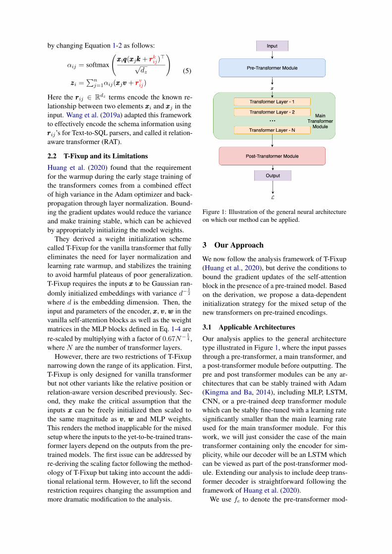
Figure 1: Illustration of the general neural architectureon which our method can be applied.

3 Our Approach

We now follow the analysis framework of T-Fixup(Huang et al., 2020), but derive the conditions tobound the gradient updates of the self-attentionblock in the presence of a pre-trained model. Basedon the derivation, we propose a data-dependentinitialization strategy for the mixed setup of thenew transformers on pre-trained encodings.

3.1 Applicable ArchitecturesOur analysis applies to the general architecturetype illustrated in Figure 1, where the input passesthrough a pre-transformer, a main transformer, anda post-transformer module before outputting. Thepre and post transformer modules can be any ar-chitectures that can be stably trained with Adam(Kingma and Ba, 2014), including MLP, LSTM,CNN, or a pre-trained deep transformer modulewhich can be stably fine-tuned with a learning ratesignificantly smaller than the main learning rateused for the main transformer module. For thiswork, we will just consider the case of the maintransformer containing only the encoder for sim-plicity, while our decoder will be an LSTM whichcan be viewed as part of the post-transformer mod-ule. Extending our analysis to include deep trans-former decoder is straightforward following theframework of Huang et al. (2020).

We use fe to denote the pre-transformer mod-

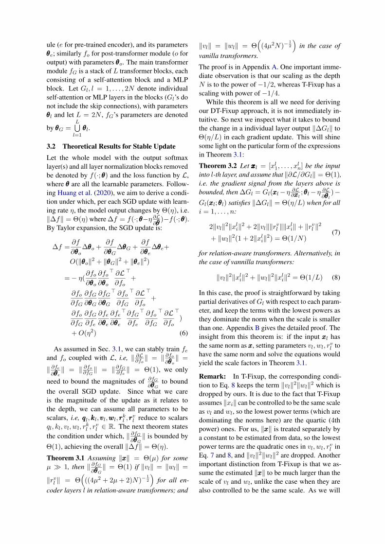
ule (e for pre-trained encoder), and its parametersθθθe; similarly fo for post-transformer module (o foroutput) with parameters θθθo. The main transformermodule fG is a stack of L transformer blocks, eachconsisting of a self-attention block and a MLPblock. Let Gl, l = 1, . . . , 2N denote individualself-attention or MLP layers in the blocks (Gl’s donot include the skip connections), with parametersθθθl and let L = 2N , fG’s parameters are denoted

by θθθG =L⋃l=1

θθθl.

3.2 Theoretical Results for Stable UpdateLet the whole model with the output softmaxlayer(s) and all layer normalization blocks removedbe denoted by f(·;θθθ) and the loss function by L,where θθθ are all the learnable parameters. Follow-ing Huang et al. (2020), we aim to derive a condi-tion under which, per each SGD update with learn-ing rate η, the model output changes by Θ(η), i.e.‖∆f‖ = Θ(η) where ∆f = f(·;θθθ−η ∂L

∂θθθ)−f(·;θθθ).

By Taylor expansion, the SGD update is:

∆f =∂f

∂θθθo∆θθθo +

∂f

∂θθθG∆θθθG +

∂f

∂θθθe∆θθθe+

O(‖θθθo‖2 + ‖θθθG‖2 + ‖θθθe‖2)

=− η(∂fo∂θθθo

∂fo∂θθθo

> ∂L∂fo

>+

∂fo∂fG

∂fG∂θθθG

∂fG∂θθθG

> ∂fo∂fG

> ∂L∂fo

>+

∂fo∂fG

∂fG∂fe

∂fe∂θθθe

∂fe∂θθθe

>∂fG∂fe

> ∂fo∂fG

> ∂L∂fo

>)

+O(η2) (6)

As assumed in Sec. 3.1, we can stably train feand fo coupled with L, i.e, ‖ ∂L

∂fo‖ = ‖ ∂fo

∂θθθo‖ =

‖ ∂fe∂θθθe‖ = ‖ ∂fo∂fG

‖ = ‖∂fG∂fe‖ = Θ(1), we only

need to bound the magnitudes of ∂fG∂θθθG

to boundthe overall SGD update. Since what we careis the magnitude of the update as it relates tothe depth, we can assume all parameters to bescalars, i.e, qqql, kkkl, vvvl,wwwl, rrr

kl , rrr

vl reduce to scalars

ql, kl, vl, wl, rkl , r

vl ∈ R. The next theorem states

the condition under which, ‖ ∂fG∂θθθG‖ is bounded by

Θ(1), achieving the overall ‖∆f‖ = Θ(η).

Theorem 3.1 Assuming ‖xxx‖ = Θ(µ) for someµ � 1, then ‖ ∂fG

∂θθθG‖ = Θ(1) if ‖vl‖ = ‖wl‖ =

‖rvl ‖ = Θ(

((4µ2 + 2µ+ 2)N)−12

)for all en-

coder layers l in relation-aware transformers; and

‖vl‖ = ‖wl‖ = Θ(

(4µ2N)−12

)in the case of

vanilla transformers.

The proof is in Appendix A. One important imme-diate observation is that our scaling as the depthN is to the power of −1/2, whereas T-Fixup has ascaling with power of −1/4.

While this theorem is all we need for derivingour DT-Fixup approach, it is not immediately in-tuitive. So next we inspect what it takes to boundthe change in a individual layer output ‖∆Gl‖ toΘ(η/L) in each gradient update. This will shinesome light on the particular form of the expressionsin Theorem 3.1:

Theorem 3.2 Let xxxxxxxxxl = [xl1, . . . , xln] be the input

into l-th layer, and assume that ‖∂L/∂Gl‖ = Θ(1),i.e. the gradient signal from the layers above isbounded, then ∆Gl = Gl(xxxl−η ∂L

∂xxxl;θθθl−η ∂L

∂θθθl)−

Gl(xxxl;θθθl) satisfies ‖∆Gl‖ = Θ(η/L) when for alli = 1, . . . , n:

2‖vl‖2‖xli‖2 + 2‖vl‖‖rvl ‖‖xli‖+ ‖rvl ‖2

+ ‖wl‖2(1 + 2‖xli‖2) = Θ(1/N)(7)

for relation-aware transformers. Alternatively, inthe case of vannilla transformers:

‖vl‖2‖xli‖2 + ‖wl‖2‖xli‖2 = Θ(1/L) (8)

In this case, the proof is straightforward by takingpartial derivatives ofGl with respect to each param-eter, and keep the terms with the lowest powers asthey dominate the norm when the scale is smallerthan one. Appendix B gives the detailed proof. Theinsight from this theorem is: if the input xxxl hasthe same norm as xxx, setting parameters vl, wl, r

vl to

have the same norm and solve the equations wouldyield the scale factors in Theorem 3.1.

Remark: In T-Fixup, the corresponding condi-tion to Eq. 8 keeps the term ‖vl‖2‖wl‖2 which isdropped by ours. It is due to the fact that T-Fixupassumes ‖xi‖ can be controlled to be the same scaleas vl and wl, so the lowest power terms (which aredominating the norms here) are the quartic (4thpower) ones. For us, ‖xxx‖ is treated separately bya constant to be estimated from data, so the lowestpower terms are the quadratic ones in vl, wl, r

vl in

Eq. 7 and 8, and ‖vl‖2‖wl‖2 are dropped. Anotherimportant distinction from T-Fixup is that we as-sume the estimated ‖xxx‖ to be much larger than thescale of vl and wl, unlike the case when they arealso controlled to be the same scale. As we will

see next, these changes imply our proposed methodemploys more aggressive scaling for initializationas compared to T-Fixup, and the assumption that‖xxx‖ has larger scale is satisfied naturally.

3.3 Proposed Method: DT-Fixup

Unlike previous works (Zhang et al., 2019b; Huanget al., 2020), appropriate initialization is not enoughto ensure Eq. 7 and 8 during the early stage of thetraining. This is due to the fact that the input xxxoften depends on the pre-trained model weightsinstead of being initialized by ourselves. Empiri-cally, we observe that the input norm ‖xxx‖ are rela-tively stable throughout the training but difficultyto control directly by re-scaling. Based on this ob-servation, we treat ‖xxx‖ as a constant and estimateit by a forward pass on all the training examplesas µ = maxj [‖xxxj‖]. We then use this estimated µin the factors of Theorem 3.1 to obtain the scalingneeded for initialization. Since parameters of alllayers are initialized to the same scale, we dropindex l for brevity in this section. In practice, µ ison the order of 10 for pre-trained models, hencev, w and rvi are naturally two orders of magnitudesmaller. DT-Fixup is described as follows:

• Apply Xavier initialization (Glorot and Ben-gio, 2010) on all free parameters exceptloaded weights from the pre-training models;

• Remove the learning rate warm-up and alllayer normalization in the transformer layers,except those in the pre-trained transformer;

• Forward-pass on all the training examples toget the max input norm µ = maxj [‖xxxj‖];

• Inside each transformer layer, scale v, w, rv

in the attention block and weight matrices inthe MLP block by (N ∗ (4µ2 + 2µ + 2))−

12

for relation-aware transformer layer; or scalev, w in the attention block and weight ma-trices in the MLP block by N−

12 /(2µ) for

vanilla transformer layer.

4 Applications

4.1 Text-to-SQL Semantic Parsing

We first apply DT-Fixup on the task of cross-domain Text-to-SQL semantic parsing. Given anunseen schema S for a database during training,our goal is to translate the natural question Q tothe target SQL T . The correct prediction depends

on the interplay between the questions and theschema structures and the generalization over un-seen schemas during inference. As a result, rea-soning and structural understanding are crucial toperform well on this task, especially for the morechallenging cases. We denote our baseline modelas SQL-SP3 and henceforth.

Implementation. For modeling Text-to-SQLgeneration, we adopt the encoder-decoder frame-work which can be directly fit into the architectureshown in Fig. 1. First, the pre-transformer modulefe is a pre-trained language model which embedsthe inputs Q and S into joint representations xxxifor each column, table si ∈ S and question wordqi ∈ Q respectively. The joint representations arepassed into a sequence of N relation-aware trans-former layers. The post-transformer module fo isa grammar-guided LSTM decoder, which uses thetransformer output yyyi to predict the target SQL T .We follow prior arts (Wang et al., 2019a; Guo et al.,2019; Yin and Neubig, 2018) to implement SQL-SP. The implementation details and hyperparametersettings are described in Appendix C.

Dataset. We evaluate SQL-SP on Spider (Yuet al., 2018), a complex and cross-domain Text-to-SQL semantic parsing benchmark. The datasetsize is relatively small by deep learning standards,with only 10,181 questions and 5,693 queries cov-ering 200 databases in 138 domains.

4.2 Logical Reading Comprehension

The second task where we apply DT-Fixup is multi-choice reading comprehension requiring logicalreasoning. Given a context, a question and four op-tions, the task is to select the right or most suitableanswer. Rather than extracting relevant informa-tion from a long context, this task relies heavily onthe logical reasoning ability of the models.

Implementation. On top of the pre-trained en-codings of the input context, question and options,a stack of N vanilla transformer layers are addedbefore the final linear layer which gives the pre-dictions. The implementation details and hyper-paramter settings are described in Appendix D

Dataset. We evaluate on ReClor (Yu et al.,2020b), a newly curated reading comprehensiondataset requiring logical reasoning. The datasetcontains logical reasoning questions taken from

3SQL Semantic Parser.

standardized exams (such as GMAT and LSAT)that are designed for students who apply for admis-sion to graduate schools. Similar to Spider, thisdataset is also small, with only 6,139 questions.

5 Experiments

All the experiments in this paper are conductedwith a signle 16GB Nvidia P100 GPU.

5.1 Semantic Parsing: Spider Results

As the test set of Spider is only accessible throughan evaluation server, most of our analyses are per-formed on the development set. We use the exactmatch accuracy4 on all examples following Yu et al.(2018), which omits evaluation of generated valuesin the SQL queries.

Model Dev TestRAT-SQL v3 + BERT (Wang et al., 2019a) 69.7 65.6RAT-SQL + GraPPa (Yu et al., 2020a) 73.4 69.6RAT-SQL + GAP (Shi et al., 2020) 71.8 69.7RAT-SQL + GraPPa + GP (Zhao et al., 2021) 72.8 69.8SGA-SQL + GAP (Anonymous) 73.1 70.1RAT-SQL + GraPPa + Adv (Anonymous) 75.5 70.5DT-Fixup SQL-SP + RobERTa (ours) 75.0 70.9

Table 1: Our accuracy on the Spider development andtest sets, as compared to the other approaches at the topof the Spider leaderboard as of May 27th, 2021.

Model N Pretrain Epochs Acc.RAT-SQL + BERT 8 ∼ 200 69.7RAT-SQL + RoBERTa 8 ∼ 200 69.6RAT-SQL + GraPPa 8 X ∼ 100 73.4RAT-SQL + GAP 8 X ∼ 200 71.8SQL-SP + RoBERTa 8 60 66.9+ More Epochs 8 100 69.2+ DT-Fixup 8 60 73.5+ DT-Fixup & More Layers 24 60 75.0+ T-Fixup∗ & More Layers 24 60 Failed

Table 2: Comparisons with the models leveraging re-lational transformers on the Spider development set.Pretrain here denotes task-specific pre-training, whichleverges additional data and tasks, and is orthorgonalto our contribution. Not only we converge faster andreach better solution, simply training longer from thesame baseline cannot close the performance gap. ∗Wedrop the constraints on the inputs to allow the applica-tion of T-Fixup in the mixed setup.

We present our results on the Spider leader-board5 in Table 1, where SQL-SP trained with DT-Fixup outperforms all the other approaches and

4We use the evaluation script provided in this repo:https://github.com/taoyds/spider

5https://yale-lily.github.io/spider

achieves the new state of the art performance. No-tably, the top four submissions on the previousleaderboard are all occupied by models leveragingrelation-aware transformers and task-specific pre-training. Table 2 compares our proposed modelswith the publicly available works. With enoughtraining steps, our baseline model trained with thestandard optimization strategy achieves the samelevel of performance as compared to RAT-SQL.However, models trained with standard optimiza-tion strategy obtain much lower performance withthe same epochs6 of training as compared to modelstrained with DT-Fixup and require more trainingsteps to achieve the best accuracy. At the sametime, by adding more relation-aware transformerlayers, further gains can be obtained for modelstrained with DT-Fixup, which achieves the state-of-the-art performance without any task-specificpre-training on additional data sources. As men-tioned in Section 2.2, in the mixed setup, there isno way to apply T-Fixup as it was originally pro-posed. The closest thing to compare is to drop itsconstraints on the inputs, but training then becomeshighly unstable and fails to converge 4 times outof 5 runs. These results demonstrate the necessityand effectiveness of DT-Fixup to improve and ac-celerate the transformer training for Text-to-SQLparsers.

Model Easy Medium Hard Extra AllDevRAT-SQL 86.4 73.6 62.1 42.9 69.7Bridge (ensemble) 89.1 71.7 62.1 51.8 71.1DT-Fixup SQL-SP 91.9 80.9 60.3 48.8 75.0TestRAT-SQL 83.0 71.3 58.3 38.4 65.6Bridge (ensemble) 85.3 73.4 59.6 40.3 67.5DT-Fixup SQL-SP 87.2 77.5 60.9 46.8 70.9

Table 3: Breakdown of Spider accuracy by hardness.

Table 3 shows the accuracy of our best modelas compared to other approaches7 with differentlevel of hardness defined by Yu et al. (2018). Wecan see that a large portion of the improvement ofour model comes from the medium level on bothdev and test set. Interestingly, while our modelobtains similar performance for the extra hard levelon the dev set, our model performs significantlybetter on the unseen test set. As most of the extra

6One epoch iterates over the whole training set once. Wanget al. (2019a) trained with a batch size of 20 for 90,000 steps,which is around 200 epochs on the Spider training set. Yuet al. (2020a) trained with a batch size of 24 for 40, 000 steps,which is around 100 epochs on the Spider training set.

7We choose the top two submissions which also report thebreakdown of the accuracy on the test set.

hard cases involves implicit reasoning steps andcomplicated structures, it shows that our proposedmodels possess stronger reasoning and structuralunderstanding ability, yielding better generalizationover unseen domains and database schemas.

5.2 Reading Comprehension: ReClor Results

Model Dev Testno extra layers∗ (Yu et al., 2020b) 62.6 55.6no extra layers 63.6 56.24 extra layers 66.2 58.24 extra layers + DT-Fixup 66.8 61.0

Table 4: Our accuracy on ReClor. Star∗ is the best base-line model result reported in (Yu et al., 2020b) withoutusing the additional RACE dataset (Lai et al., 2017).

For ReClor, we choose the best model in Yuet al. (2020b) as the baseline which employs a lin-ear classifier on top of RoBERTa. From the re-sults presented in Table 4, we can see that simplystacking additional vanilla transformer layers out-performs the baseline and adding DT-Fixup furtherimproves the accuracy, which ranks the second onthe public leaderboard at the time of this submis-sion8. The result further validates the benefit ofadding extra transformer layers and the effective-ness of DT-Fixup.

5.3 Ablation StudiesFor fair comparisons and better understanding, weconduct multiple sets of ablation with the samearchitecture and implementation to validate the ad-vantages of DT-Fixup over the standard optimiza-tion strategy. Note that, the batch sizes in our exper-iments are relatively small (16 for Spider and 24 forReClor) due to the size of the pre-trained models,while batch sizes for masked language modelling(Liu et al., 2019b) and machine translation (Huanget al., 2020) are commonly larger than 1024.

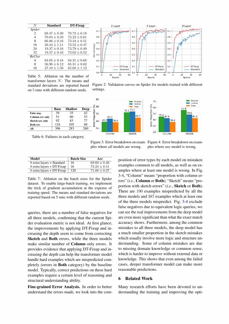
Deeper Models. As we can see from Table 5, thestandard optimization strategy fails completely totrain deep transformers whose depths are largerthan 8 on both Spider and ReClor, showing that itstruggles to properly train the transformer modelas the depth increases. At the same time, DT-Fixupcan successfully train deeper transformers up to 32layers and consistently achieves better performancethan models trained by the standard optimizationstrategy with the same depth on both Spider andReClor. With DT-Fixup, deep models generally

8https://eval.ai/web/challenges/challenge-page/503/

achieve better performance than the shallow oneseven there are only thousands of training exam-ples. It contradicts the common belief that increas-ing depth of the transformer model is helpful onlywhen there are enough training data.

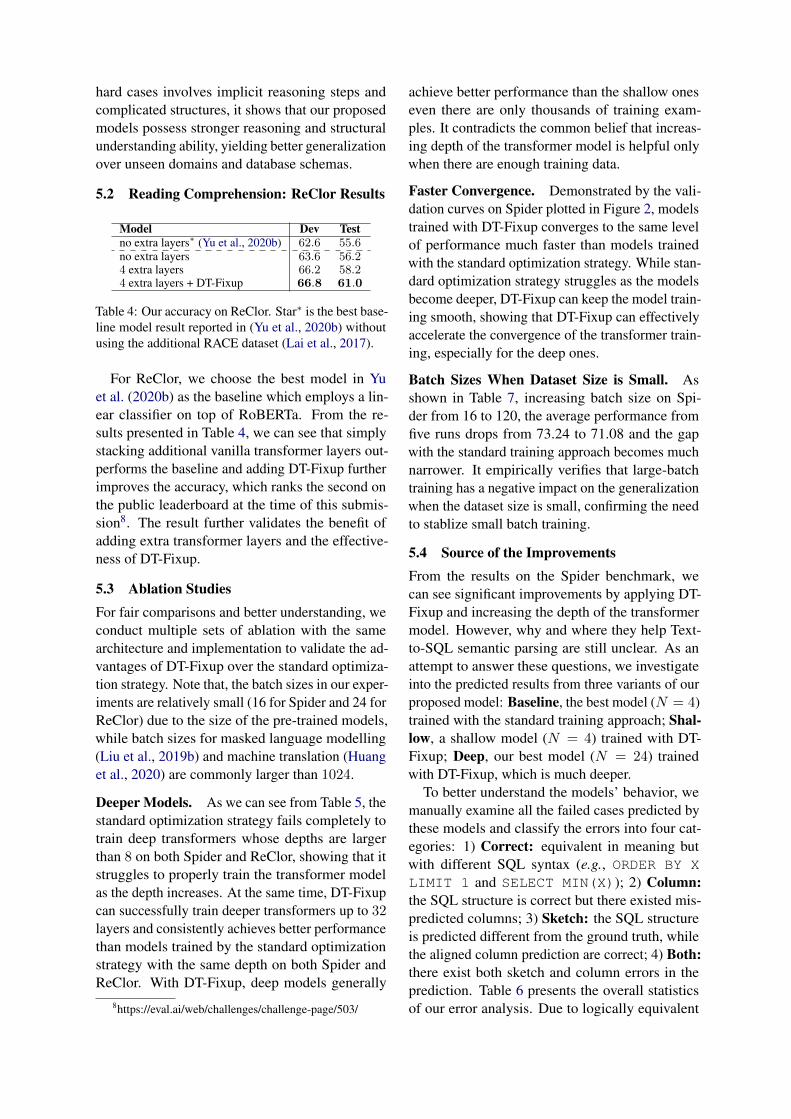
Faster Convergence. Demonstrated by the vali-dation curves on Spider plotted in Figure 2, modelstrained with DT-Fixup converges to the same levelof performance much faster than models trainedwith the standard optimization strategy. While stan-dard optimization strategy struggles as the modelsbecome deeper, DT-Fixup can keep the model train-ing smooth, showing that DT-Fixup can effectivelyaccelerate the convergence of the transformer train-ing, especially for the deep ones.

Batch Sizes When Dataset Size is Small. Asshown in Table 7, increasing batch size on Spi-der from 16 to 120, the average performance fromfive runs drops from 73.24 to 71.08 and the gapwith the standard training approach becomes muchnarrower. It empirically verifies that large-batchtraining has a negative impact on the generalizationwhen the dataset size is small, confirming the needto stablize small batch training.

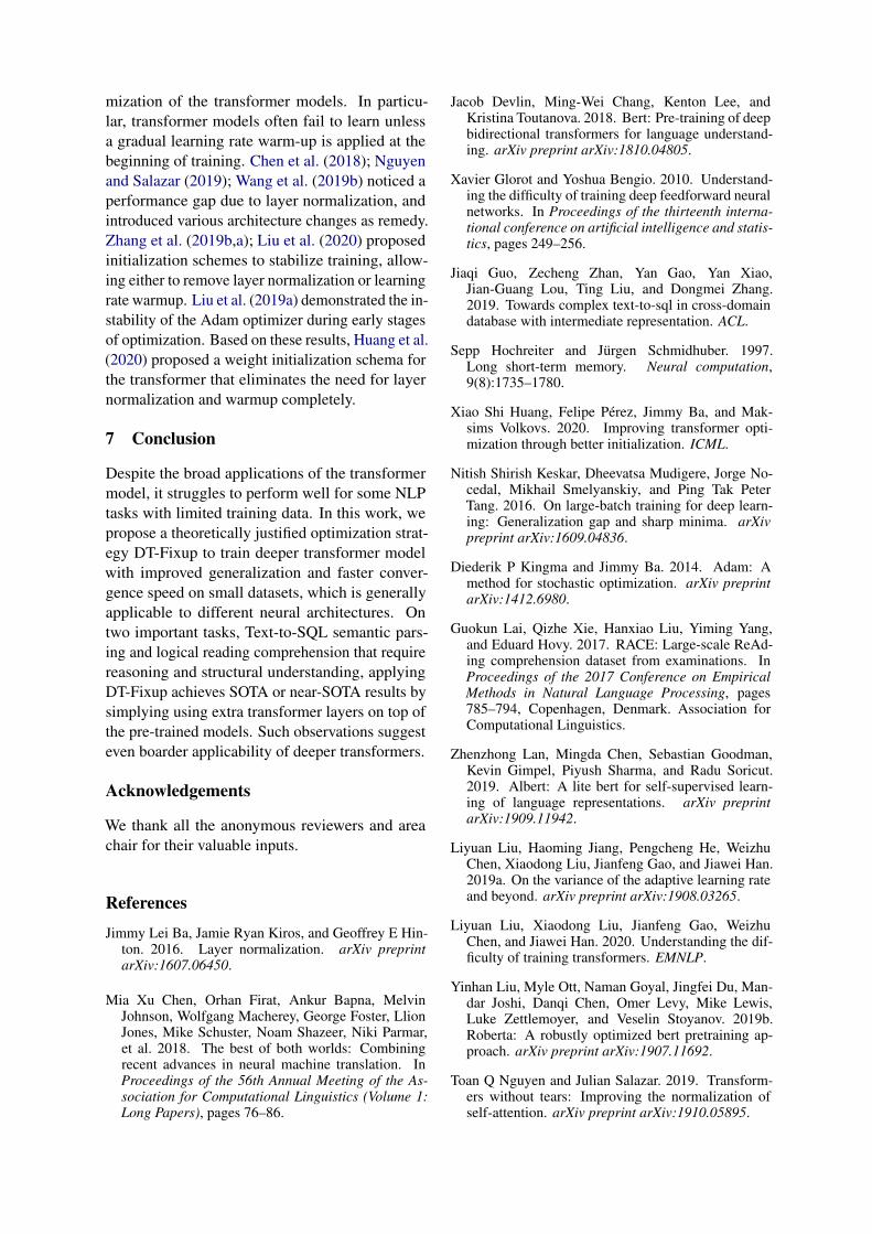
5.4 Source of the ImprovementsFrom the results on the Spider benchmark, wecan see significant improvements by applying DT-Fixup and increasing the depth of the transformermodel. However, why and where they help Text-to-SQL semantic parsing are still unclear. As anattempt to answer these questions, we investigateinto the predicted results from three variants of ourproposed model: Baseline, the best model (N = 4)trained with the standard training approach; Shal-low, a shallow model (N = 4) trained with DT-Fixup; Deep, our best model (N = 24) trainedwith DT-Fixup, which is much deeper.

To better understand the models’ behavior, wemanually examine all the failed cases predicted bythese models and classify the errors into four cat-egories: 1) Correct: equivalent in meaning butwith different SQL syntax (e.g., ORDER BY XLIMIT 1 and SELECT MIN(X)); 2) Column:the SQL structure is correct but there existed mis-predicted columns; 3) Sketch: the SQL structureis predicted different from the ground truth, whilethe aligned column prediction are correct; 4) Both:there exist both sketch and column errors in theprediction. Table 6 presents the overall statisticsof our error analysis. Due to logically equivalent

N Standard DT-FixupSpider

2 69.47± 0.30 70.73± 0.184 70.04± 0.33 72.22± 0.618 66.86± 0.16 73.24± 0.51

16 20.44± 1.11 73.52± 0.4724 19.37± 0.16 73.79± 0.4932 19.57± 0.43 73.02± 0.52

ReClor4 64.05± 0.44 64.31± 0.688 56.96± 6.12 65.31± 0.62

16 27.10± 1.50 65.68± 1.12

Table 5: Ablation on the number oftransformer layers N . The means andstandard deviations are reported basedon 5 runs with different random seeds.

Figure 2: Validation curves on Spider for models trained with differentsettings.

Base Shallow DeepFalse neg. 39 35 42Column err. only 51 60 53Sketch err. only 92 83 77Both err. 124 105 88All 306 283 260

Table 6: Failures in each category.Figure 3: Error breakdown on exam-ples where all models are wrong.

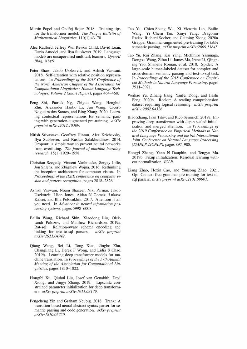
Figure 4: Error breakdown on exam-ples where any model is wrong.

Model Batch Size Acc8 extra layers + Standard 16 69.60± 0.408 extra layers + DT-Fixup 16 73.24± 0.518 extra layers + DT-Fixup 120 71.08± 0.37

Table 7: Ablation on the batch sizes for the Spiderdataset. To enable large-batch training, we implementthe trick of gradient accumulation at the expense oftraining speed. The means and standard deviations arereported based on 5 runs with different random seeds.

queries, there are a number of false negatives forall three models, confirming that the current Spi-der evaluation metric is not ideal. At first glance,the improvements by applying DT-Fixup and in-creasing the depth seem to come from correctingSketch and Both errors, while the three modelsmake similar number of Column only errors. Itprovides evidence that applying DT-Fixup and in-creasing the depth can help the transformer modelhandle hard examples which are mispredicted com-pletely (errors in Both category) by the baselinemodel. Typically, correct predictions on these hardexamples require a certain level of reasoning andstructural understanding ability.

Fine-grained Error Analysis. In order to betterunderstand the errors made, we look into the com-

position of error types by each model on mistakenexamples common to all models, as well as on ex-amples where at least one model is wrong. In Fig.3-4, “Column” means “proportion with column er-rors” (i.e., Column or Both); “Sketch” means “pro-portion with sketch errors” (i.e., Sketch or Both).There are 190 examples mispredicted by all thethree models and 387 examples which at least oneof the three models mispredict. Fig. 3-4 excludefalse negatives due to equivalent logic queries, wecan see the real improvements from the deep modelare even more significant than what the exact matchaccuracy shows. Furthermore, among the commonmistakes to all three models, the deep model hasa much smaller proportion in the sketch mistakeswhich usually involve more logic and structure un-derstanding. Some of column mistakes are dueto missing domain knowledge or common sense,which is harder to improve without external data orknowledge. This shows that even among the failedcases, deeper transformer model can make morereasonable predictions.

6 Related Work

Many research efforts have been devoted to un-derstanding the training and improving the opti-

mization of the transformer models. In particu-lar, transformer models often fail to learn unlessa gradual learning rate warm-up is applied at thebeginning of training. Chen et al. (2018); Nguyenand Salazar (2019); Wang et al. (2019b) noticed aperformance gap due to layer normalization, andintroduced various architecture changes as remedy.Zhang et al. (2019b,a); Liu et al. (2020) proposedinitialization schemes to stabilize training, allow-ing either to remove layer normalization or learningrate warmup. Liu et al. (2019a) demonstrated the in-stability of the Adam optimizer during early stagesof optimization. Based on these results, Huang et al.(2020) proposed a weight initialization schema forthe transformer that eliminates the need for layernormalization and warmup completely.

7 Conclusion

Despite the broad applications of the transformermodel, it struggles to perform well for some NLPtasks with limited training data. In this work, wepropose a theoretically justified optimization strat-egy DT-Fixup to train deeper transformer modelwith improved generalization and faster conver-gence speed on small datasets, which is generallyapplicable to different neural architectures. Ontwo important tasks, Text-to-SQL semantic pars-ing and logical reading comprehension that requirereasoning and structural understanding, applyingDT-Fixup achieves SOTA or near-SOTA results bysimplying using extra transformer layers on top ofthe pre-trained models. Such observations suggesteven boarder applicability of deeper transformers.

Acknowledgements

We thank all the anonymous reviewers and areachair for their valuable inputs.

References

Jimmy Lei Ba, Jamie Ryan Kiros, and Geoffrey E Hin-ton. 2016. Layer normalization. arXiv preprintarXiv:1607.06450.

Mia Xu Chen, Orhan Firat, Ankur Bapna, MelvinJohnson, Wolfgang Macherey, George Foster, LlionJones, Mike Schuster, Noam Shazeer, Niki Parmar,et al. 2018. The best of both worlds: Combiningrecent advances in neural machine translation. InProceedings of the 56th Annual Meeting of the As-sociation for Computational Linguistics (Volume 1:Long Papers), pages 76–86.

Jacob Devlin, Ming-Wei Chang, Kenton Lee, andKristina Toutanova. 2018. Bert: Pre-training of deepbidirectional transformers for language understand-ing. arXiv preprint arXiv:1810.04805.

Xavier Glorot and Yoshua Bengio. 2010. Understand-ing the difficulty of training deep feedforward neuralnetworks. In Proceedings of the thirteenth interna-tional conference on artificial intelligence and statis-tics, pages 249–256.

Jiaqi Guo, Zecheng Zhan, Yan Gao, Yan Xiao,Jian-Guang Lou, Ting Liu, and Dongmei Zhang.2019. Towards complex text-to-sql in cross-domaindatabase with intermediate representation. ACL.

Sepp Hochreiter and Jurgen Schmidhuber. 1997.Long short-term memory. Neural computation,9(8):1735–1780.

Xiao Shi Huang, Felipe Perez, Jimmy Ba, and Mak-sims Volkovs. 2020. Improving transformer opti-mization through better initialization. ICML.

Nitish Shirish Keskar, Dheevatsa Mudigere, Jorge No-cedal, Mikhail Smelyanskiy, and Ping Tak PeterTang. 2016. On large-batch training for deep learn-ing: Generalization gap and sharp minima. arXivpreprint arXiv:1609.04836.

Diederik P Kingma and Jimmy Ba. 2014. Adam: Amethod for stochastic optimization. arXiv preprintarXiv:1412.6980.

Guokun Lai, Qizhe Xie, Hanxiao Liu, Yiming Yang,and Eduard Hovy. 2017. RACE: Large-scale ReAd-ing comprehension dataset from examinations. InProceedings of the 2017 Conference on EmpiricalMethods in Natural Language Processing, pages785–794, Copenhagen, Denmark. Association forComputational Linguistics.

Zhenzhong Lan, Mingda Chen, Sebastian Goodman,Kevin Gimpel, Piyush Sharma, and Radu Soricut.2019. Albert: A lite bert for self-supervised learn-ing of language representations. arXiv preprintarXiv:1909.11942.

Liyuan Liu, Haoming Jiang, Pengcheng He, WeizhuChen, Xiaodong Liu, Jianfeng Gao, and Jiawei Han.2019a. On the variance of the adaptive learning rateand beyond. arXiv preprint arXiv:1908.03265.

Liyuan Liu, Xiaodong Liu, Jianfeng Gao, WeizhuChen, and Jiawei Han. 2020. Understanding the dif-ficulty of training transformers. EMNLP.

Yinhan Liu, Myle Ott, Naman Goyal, Jingfei Du, Man-dar Joshi, Danqi Chen, Omer Levy, Mike Lewis,Luke Zettlemoyer, and Veselin Stoyanov. 2019b.Roberta: A robustly optimized bert pretraining ap-proach. arXiv preprint arXiv:1907.11692.

Toan Q Nguyen and Julian Salazar. 2019. Transform-ers without tears: Improving the normalization ofself-attention. arXiv preprint arXiv:1910.05895.

Martin Popel and Ondrej Bojar. 2018. Training tipsfor the transformer model. The Prague Bulletin ofMathematical Linguistics, 110(1):43–70.

Alec Radford, Jeffrey Wu, Rewon Child, David Luan,Dario Amodei, and Ilya Sutskever. 2019. Languagemodels are unsupervised multitask learners. OpenAIBlog, 1(8):9.

Peter Shaw, Jakob Uszkoreit, and Ashish Vaswani.2018. Self-attention with relative position represen-tations. In Proceedings of the 2018 Conference ofthe North American Chapter of the Association forComputational Linguistics: Human Language Tech-nologies, Volume 2 (Short Papers), pages 464–468.

Peng Shi, Patrick Ng, Zhiguo Wang, HenghuiZhu, Alexander Hanbo Li, Jun Wang, CiceroNogueira dos Santos, and Bing Xiang. 2020. Learn-ing contextual representations for semantic pars-ing with generation-augmented pre-training. arXivpreprint arXiv:2012.10309.

Nitish Srivastava, Geoffrey Hinton, Alex Krizhevsky,Ilya Sutskever, and Ruslan Salakhutdinov. 2014.Dropout: a simple way to prevent neural networksfrom overfitting. The journal of machine learningresearch, 15(1):1929–1958.

Christian Szegedy, Vincent Vanhoucke, Sergey Ioffe,Jon Shlens, and Zbigniew Wojna. 2016. Rethinkingthe inception architecture for computer vision. InProceedings of the IEEE conference on computer vi-sion and pattern recognition, pages 2818–2826.

Ashish Vaswani, Noam Shazeer, Niki Parmar, JakobUszkoreit, Llion Jones, Aidan N Gomez, ŁukaszKaiser, and Illia Polosukhin. 2017. Attention is allyou need. In Advances in neural information pro-cessing systems, pages 5998–6008.

Bailin Wang, Richard Shin, Xiaodong Liu, Olek-sandr Polozov, and Matthew Richardson. 2019a.Rat-sql: Relation-aware schema encoding andlinking for text-to-sql parsers. arXiv preprintarXiv:1911.04942.

Qiang Wang, Bei Li, Tong Xiao, Jingbo Zhu,Changliang Li, Derek F Wong, and Lidia S Chao.2019b. Learning deep transformer models for ma-chine translation. In Proceedings of the 57th AnnualMeeting of the Association for Computational Lin-guistics, pages 1810–1822.

Hongfei Xu, Qiuhui Liu, Josef van Genabith, DeyiXiong, and Jingyi Zhang. 2019. Lipschitz con-strained parameter initialization for deep transform-ers. arXiv preprint arXiv:1911.03179.

Pengcheng Yin and Graham Neubig. 2018. Tranx: Atransition-based neural abstract syntax parser for se-mantic parsing and code generation. arXiv preprintarXiv:1810.02720.

Tao Yu, Chien-Sheng Wu, Xi Victoria Lin, BailinWang, Yi Chern Tan, Xinyi Yang, DragomirRadev, Richard Socher, and Caiming Xiong. 2020a.Grappa: Grammar-augmented pre-training for tablesemantic parsing. arXiv preprint arXiv:2009.13845.

Tao Yu, Rui Zhang, Kai Yang, Michihiro Yasunaga,Dongxu Wang, Zifan Li, James Ma, Irene Li, Qingn-ing Yao, Shanelle Roman, et al. 2018. Spider: Alarge-scale human-labeled dataset for complex andcross-domain semantic parsing and text-to-sql task.In Proceedings of the 2018 Conference on Empiri-cal Methods in Natural Language Processing, pages3911–3921.

Weihao Yu, Zihang Jiang, Yanfei Dong, and JiashiFeng. 2020b. Reclor: A reading comprehensiondataset requiring logical reasoning. arXiv preprintarXiv:2002.04326.

Biao Zhang, Ivan Titov, and Rico Sennrich. 2019a. Im-proving deep transformer with depth-scaled initial-ization and merged attention. In Proceedings ofthe 2019 Conference on Empirical Methods in Nat-ural Language Processing and the 9th InternationalJoint Conference on Natural Language Processing(EMNLP-IJCNLP), pages 897–908.

Hongyi Zhang, Yann N Dauphin, and Tengyu Ma.2019b. Fixup initialization: Residual learning with-out normalization. ICLR.

Liang Zhao, Hexin Cao, and Yunsong Zhao. 2021.Gp: Context-free grammar pre-training for text-to-sql parsers. arXiv preprint arXiv:2101.09901.

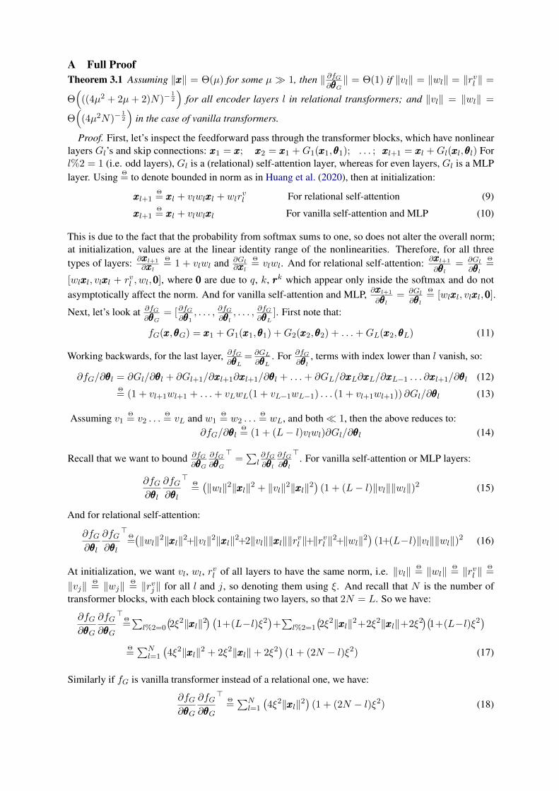
A Full ProofTheorem 3.1 Assuming ‖xxx‖ = Θ(µ) for some µ � 1, then ‖ ∂fG

∂θθθG‖ = Θ(1) if ‖vl‖ = ‖wl‖ = ‖rvl ‖ =

Θ(

((4µ2 + 2µ+ 2)N)−12

)for all encoder layers l in relational transformers; and ‖vl‖ = ‖wl‖ =

Θ(

(4µ2N)−12

)in the case of vanilla transformers.

Proof. First, let’s inspect the feedforward pass through the transformer blocks, which have nonlinearlayers Gl’s and skip connections: xxx1 = xxx; xxx2 = xxx1 +G1(xxx1, θθθ1); . . . ; xxxl+1 = xxxl +Gl(xxxl, θθθl) Forl%2 = 1 (i.e. odd layers), Gl is a (relational) self-attention layer, whereas for even layers, Gl is a MLPlayer. Using Θ

= to denote bounded in norm as in Huang et al. (2020), then at initialization:

xxxl+1Θ= xxxl + vlwlxxxl + wlr

vl For relational self-attention (9)

xxxl+1Θ= xxxl + vlwlxxxl For vanilla self-attention and MLP (10)

This is due to the fact that the probability from softmax sums to one, so does not alter the overall norm;at initialization, values are at the linear identity range of the nonlinearities. Therefore, for all threetypes of layers: ∂xxxl+1

∂xxxl

Θ= 1 + vlwl and ∂Gl

∂xxxl

Θ= vlwl. And for relational self-attention: ∂xxxl+1

∂θθθl= ∂Gl

∂θθθlΘ=

[wlxxxl, vlxxxl + rvl , wl,000], where 000 are due to q, k, rrrk which appear only inside the softmax and do notasymptotically affect the norm. And for vanilla self-attention and MLP, ∂xxxl+1

∂θθθl= ∂Gl

∂θθθlΘ= [wlxxxl, vlxxxl,000].

Next, let’s look at ∂fG∂θθθG

= [∂fG∂θθθ1

, . . . , ∂fG∂θθθl

, . . . , ∂fG∂θθθL

]. First note that:

fG(xxx,θθθG) = xxx1 +G1(xxx1, θθθ1) +G2(xxx2, θθθ2) + . . .+GL(xxx2, θθθL) (11)

Working backwards, for the last layer, ∂fG∂θθθL

= ∂GL

∂θθθL. For ∂fG

∂θθθl, terms with index lower than l vanish, so:

∂fG/∂θθθl = ∂Gl/∂θθθl + ∂Gl+1/∂xxxl+1∂xxxl+1/∂θθθl + . . .+ ∂GL/∂xxxL∂xxxL/∂xxxL−1 . . . ∂xxxl+1/∂θθθl (12)Θ= (1 + vl+1wl+1 + . . .+ vLwL(1 + vL−1wL−1) . . . (1 + vl+1wl+1)) ∂Gl/∂θθθl (13)

Assuming v1Θ= v2 . . .

Θ= vL and w1

Θ= w2 . . .

Θ= wL, and both� 1, then the above reduces to:

∂fG/∂θθθlΘ= (1 + (L− l)vlwl)∂Gl/∂θθθl (14)

Recall that we want to bound ∂fG∂θθθG

∂fG∂θθθG

>=∑

l∂fG∂θθθl

∂fG∂θθθl

>. For vanilla self-attention or MLP layers:

∂fG∂θθθl

∂fG∂θθθl

>Θ=(‖wl‖2‖xxxl‖2 + ‖vl‖2‖xxxl‖2

)(1 + (L− l)‖vl‖‖wl‖)2 (15)

And for relational self-attention:

∂fG∂θθθl

∂fG∂θθθl

>Θ=(‖wl‖2‖xxxl‖2+‖vl‖2‖xxxl‖2+2‖vl‖‖xxxl‖‖rvl ‖+‖rvl ‖2+‖wl‖2

)(1+(L−l)‖vl‖‖wl‖)2 (16)

At initialization, we want vl, wl, rvl of all layers to have the same norm, i.e. ‖vl‖Θ= ‖wl‖

Θ= ‖rvl ‖

Θ=

‖vj‖Θ= ‖wj‖

Θ= ‖rvj ‖ for all l and j, so denoting them using ξ. And recall that N is the number of

transformer blocks, with each block containing two layers, so that 2N = L. So we have:

∂fG∂θθθG

∂fG∂θθθG

>Θ=∑

l%2=0

(2ξ2‖xxxl‖2

) (1+(L−l)ξ2

)+∑

l%2=1

(2ξ2‖xxxl‖2+2ξ2‖xxxl‖+2ξ2

)(1+(L−l)ξ2

)Θ=∑N

l=1

(4ξ2‖xxxl‖2 + 2ξ2‖xxxl‖+ 2ξ2

)(1 + (2N − l)ξ2) (17)

Similarly if fG is vanilla transformer instead of a relational one, we have:

∂fG∂θθθG

∂fG∂θθθG

>Θ=∑N

l=1

(4ξ2‖xxxl‖2

)(1 + (2N − l)ξ2) (18)

The only variable that still depends on l is xxxl, which by expanding the recursion in Eq. 9-10, gives:

xxxlΘ= (1 + ξ2)lxxx

Θ= (1 + lξ2 + Θ(ξ4))xxx For vanillla transformer (19)

xxxlΘ= (1 + ξ2)lxxx+ l/2ξ2

Θ= (1 + lξ2 + Θ(ξ4))xxx+ l/2ξ2 For relational transformer (20)

Now let ‖xxx‖ Θ= µ , and we have assumed that µ � 1, which is very common for output of pre-trained

encoders, and due to the high dimensionality. And let

ξ =(N(4µ2 + 2µ+ 2)

)− 12 (21)

Then substituting it into Eq. 19-20, we have xxxlΘ= xxx for all types of layers. Similarly, plugging Eq. 21 into

the expression (1 + (2N − l)ξ2) in Eq. 17 yields (1 + (2N − l)ξ2) Θ= 1, together with xxxl

Θ= xxx, and Eq.

21, Eq. 17 becomes:

∂fG∂θθθG

∂fG∂θθθG

>Θ=∑N

l=1

4µ2

N (4µ2 + 2µ+ 2)+

2µ

N (4µ2 + 2µ+ 2)+

2

N (4µ2 + 2µ+ 2)

Θ=∑N

l=11/N = Θ(1)

This concludes the proof for relational transformers. For vanilla transformers, with ξ =(N(4µ2)

)− 12 ,

and following the same steps, but plugging into Eq. 18, we have ∂fG∂θθθG

∂fG∂θθθG

> Θ= 1. Q.E.D.

B Proof of Theorem 3.2For brevity, we drop the layer index. But for the relation embeddings, for clarity, we will consider theindividual components of rrrv, rrrk instead of considering the scalar case.

Proof. We will focus the self-attention layer, as the skip connection and MLP layers are analyzed inHuang et al. (2020). As mentioned in the main text, since what we care is the magnitude of the update,we assume dx = 1 and drop layer index l without loss of generality. In this case, the projection matricesqqq,kkk,vvv,www reduce to scalars q, k, v, w ∈ R. The input xxx and the relational embeddings rrrk, rrrv are n × 1vectors. For a single query input x′ ∈ xxx, the attention layer (without skip connection) is defined as follows:

G(x′) = softmax(

1√dxx′q(kxxx+ rrrk)>

)(xxxv + rrrv)w =

∑ni=1

ex′q(kxi+rki )∑n

j=1ex′q(kxj+rkj )

(xiv + rvi )w

Note that we are abusing the notation and take G to be just the self-attention layer output here. Letsi = ex

′q(kxi+rki )/∑n

j=1ex′q(kxj+rkj ) and δij = 1 if i = j and 0 otherwise, we can get:

∂G/∂k = x′qw∑n

i=1(xiv + rvi )si

(xi −

∑nj=1xjsj

)∂G/∂q = x′w

∑ni=1(xiv + rvi )si

(kxi + rki −

∑nj=1(kxj + rkj )sj

)∂G/∂rki = x′qw

(−(xiv + rvi )si +

∑nj=1(xjv + rvj )sj

); ∂G/∂v = w

∑ni=1xisi

∂G/∂w =∑n

i=1(xiv + rvi )si ; ∂G/∂rvi = wsi ; ∂G/∂xi = vwsi + w∑n

j=1∂sj/∂xi(xjv + rvj )

When xi 6= x′, we have: ∂sj∂xi

= sj(δij − si)x′qk; When xi = x′, we have: ∂sj

∂xi=

q((1 + δij)kxi + rki

)sj −

∑nt=1q

((1 + δit)kxt + rkt

)sjst Using Taylor expansion, we get that the

SGD update ∆G is proportional to the magnitude of the gradient:

∆G = −η ∂L∂G

(∂G

∂k

∂G

∂k

>+∂G

∂q

∂G

∂q

>+∂G

∂v

∂G

∂v

>+∂G

∂w

∂G

∂w

>

+∑n

i=1

∂G

∂rki

∂G

∂rki

>+∑n

i=1

∂G

∂rvi

∂G

∂rvi

>+∑n

i=1

∂G

∂xi

∂G

∂xi

>)

+O(η2)

By the assumption that ‖η ∂L∂G‖ = Θ(η), we need to bound the term inside the main parentheses by

Θ(1/L). The desired magnitude Θ(1/L) is smaller than 1 so terms with lower power are dominating.With si ≥ 0 and

∑si = 1, the following terms have the lowest power inside the main parentheses:

∂G

∂v

∂G

∂v

>= w2(

∑ni=1xisi)

2 = Θ(‖w‖2‖xi‖2), i = 1, . . . , n

∂G

∂w

∂G

∂w

>= (

∑ni=1(xiv + rvi )si)

2 = Θ(‖v‖2‖xi‖2) + 2Θ(‖v‖‖rvi ‖‖xi‖) + Θ(‖rvi ‖2), i = 1, . . . , n

∑ni=1

∂G

∂rvi

∂G

∂rvi

>= w2∑n

i=1s2i = Θ(‖w‖2).

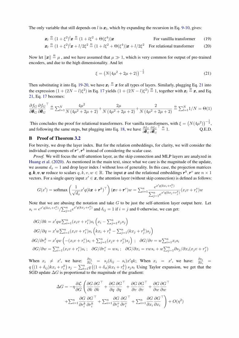
For the MLP layer, all terms related to rvi disappear, including the single Θ(‖w‖2) in the last row. Bycombining the update norm terms from both the self-attention and the MLP layers give the result. Q.E.D.Note: The above theorem and analysis applies to a single layer, not the whole transformer module ofmany layers. In order to derive the scaling factor, one needs ensure that the output scale for each block isbounded by its input scale. This indeed holds for our scheme, but the complete proof is in Sec. A.

C Implementation Details of SQL-SPGiven a schema S for a relational database, our goal is to translate the natural question Q to the targetSQL T . Here the question Q = q1 . . . q|Q| is a sequence of words, and the schema S = {s1, . . . , s|S|}consists of tables and their columns. s ∈ S can be either a table name or a column name containingwords si,1, . . . , si,|si|. Following Wang et al. (2019a), a directed graph G = 〈V, E〉 can be constructed torepresent the relations between the inputs. Its nodes V = Q ∪ S include question tokens (each labeledwith a corresponding token) and the columns and tables of the schema (each labeled with the words in itsname). The edges E are defined following Wang et al. (2019a). The target SQL T is represented as anabstract syntax tree in the context-free grammar of SQL.

C.1 EncoderFollowing (Wang et al., 2019a; Guo et al., 2019), our pre-transformer module fe leverages pre-trainedlanguage models to obtain the input X to the main transformer module. First, the sequence of words inthe question Q are concatenated with all the items (either a column or a table) in the schema S. In orderto prevent our model from leveraging potential spurious correlations based on the order of the items, theitems in the schema are concatenated in random order during training. We feed the concatenation into thepre-trained model and extract the last hidden states xxx(q)i and hhhi = hhhi,1, . . . ,hhhi,|si| for each word in Q andeach item in S respectively. For each item si in the schema, we run an additional bidirectional LSTM(BiLSTM) (Hochreiter and Schmidhuber, 1997) over the hidden states of the words in its name hhhi. Wethen add the average hidden state and the final hidden state of the BiLSTM as the schema representationsxxx(s)i . X is the set of all the obtained representations from Q ∪ S: X = (xxx

(q)1 , . . . ,xxx

(q)|Q|,xxx

(s)1 , . . . ,xxx

(s)|S|).

Along with the relational embeddings rrrk, rrrv specified by G, X is passed into the main transformer module.

C.2 Schema LinkingThe goal of schema linking is to identify the implicit relations between Q and S. The relations aredefined by whether there exist column/table references in the question to the corresponding schemacolumns/tables, given certain heuristics. Following Wang et al. (2019a), possible relations for each (i, j)where xi ∈ Q, xj ∈ S (or vice versa) can be ExactMatch, PartialMatch, or NoMatch, whichare based on name-based linking. Depending on the type of xi and xj , the above three relations arefurther expanded to four types: Question-Column, Question-Table, Column-Question, orTable-Question. We also use the value-based linking from Wang et al. (2019a) and Guo et al. (2019)to augment the ExactMatch relation by database content and external knowledge.

C.3 DecoderFor our decoder (as the post-transformer module) fo, we employ a transition-based abstract syntax decoderfollowing Yin and Neubig (2018). It requires a transition system to converts between the surface SQLand a AST-tree constructing action sequences, and can ensure grammarticality of generation. The neuralmodel then predicts the action sequences. There are three types of actions to generate the target SQL T ,

including (i) ApplyRule which applies a production rule to the last generated node; (ii) Reduce whichcompletes a leaf node; (iii) SelectColumn which chooses a column from the schema. For our transitionsystem, each column is attached with their corresponding table so that the tables in the target SQL Tcan be directly inferred from the predicted columns. As a result, action SelectTable can be omittedfrom the generation. Formally, the generation process can be formulated as Pr(T |Y) =

∏t Pr(at|a<t,Y)

where Y is the outputs of the last layer of the relational transformers. We use a parent-feeding LSTMas the decoder. The LSTM state is updated as mmmt,hhht = fLSTM([aaat−1‖zzzt−1‖hhhpt‖aaapt‖nnnpt ],mmmt−1,hhht−1),wheremmmt is the LSTM cell state, hhht is the LSTM output at step t, aaat−1 is the action embedding of theprevious step, zzzt−1 is the context feature computed using multi-head attention on hhht−1 over Y , pt is thestep corresponding to the parent AST node of the current node, and nnn is the node type embedding. ForApplyRule[R], we compute Pr(at = ApplyRule[R]|a<t, y) = softmaxR(g(zzzt)) where g(·) is a2-layer MLP. For SelectColumn, we use the memory augmented pointer net Guo et al. (2019).

C.4 RegularizationBesides using dropout (Srivastava et al., 2014) employed on X and zzzt to help regularize the model,we further apply uniform label smoothing (Szegedy et al., 2016) on the objective of predictingSelectColumn. Formally, the cross entropy for a ground-truth column c∗ we optimize becomes:(1− ε) ∗ log p(c∗) + ε/K ∗

∑c log p(c), where K is the number of columns in the schema, ε is the weight

of the label smoothing term, and p(·) , Pr(at = SelectColumn[·]|a<t, y).

C.5 Experiment ConfigurationWe choose RoBERTa (Liu et al., 2019b) as the pre-trained language models. A sequence of 24 relation-aware transformer layers are stacked on top of fe. The Adam optimizer (Kingma and Ba, 2014) with thedefault hyperparameters is used to train the model with an initial learning rate η of 4×10−4. η is annealedto 0 with 4× 10−4(1− steps/max steps)0.5. A separate learning rate is used to fine-tune the RoBERTaby multiplying η a factor of 8× 10−3. The BiLSTM to encode the schema representations has hiddensize 128 per direction. For each transformer layer, dx = dz = 256, H = 8 and the inner layer dimensionof the position-wise MLP is 1024. For the decoder, we use action embeddings of size 128, node typeembeddings of size of 64, and LSTM hidden state of size 512. We apply dropout rate of 0.6 on the inputto the relational transformers X and the context representation zzzt. The weight of the label smoothing termis set to be 0.2. We use a batch size of 16 and train 60 epochs (around 25, 000 steps). During inference,beam search is used with beam size as 5. Most of the hyperparameters are chosen following Wang et al.(2019a). We only tune the learning rate (4 × 10−4 to 8 × 10−4 with step size 1 × 10−4), dropout (0.3,0.4, 0.5, 0.6), the weight of the label smoothing ε (0.0, 0.1, 0.2) by grid search. The average runtime isaround 30 hours and the number of parameters is around 380 millions.

D Implementation Details for Logical Reading ComprehensionWe build on the code9 by Yu et al. (2020b) and use it for evaluation. For each example, the encoderembeds the input context, question and options which are then passed to the linear layer for classification.The exact input format to the encoder is “〈s〉 Context 〈/s〉〈/s〉 Question || Option 〈pad〉 . . . ”, where “||”denotes concatenation. The linear layer uses the embedding of the first token 〈s〉 for classification.

D.1 Experimental ConfigurationRoBERT is chosen as the pre-trained model, and we stack 4 transformer layers on top. The Adamoptimizer (Kingma and Ba, 2014) with ε = 10−6 and betas of (0.9, 0.98) is used. The learning rate tofinetune RoBERTa is 1× 10−5 while the learning rate for the additional transformer layers is 3× 10−4.For all models in our ablation study, the learning rate for the additional transformer layers is 1×10−4. Thelearning rate is annealed linearly to 0 with weight decay of 0.01. We use a batch size of 24 and fine-tunefor 12 epochs. For each transformer layer, dx = dz = 1024, H = 8 and the inner layer dimension of theposition-wise MLP is 2048. We use dropout rate of 0.4 on the input to the additional transformer layersand 0.1 for the linear layer. We follow the hyperparameters used in Yu et al. (2020b) for the pretrainedlanguage model. For the additional transformer layers, we only tune the dropout values (0.3, 0.4, 0.5, 0.6).The average runtime is around 6 hours and the number of parameters is around 39 millions.

9https://github.com/yuweihao/reclor