Embed Size (px)
Citation preview
OptycznaSpektroskopia Molekuł
van der WaalsaTadeusz Bancewicz
Zakład Optyki Nieliniowej, Wydział Fizyki,Uniwersytet im. Adama Mickiewicza w Poznaniu,
http://zon8.physd.amu.edu.pl/~tbancewi
10 kwietnia 2011
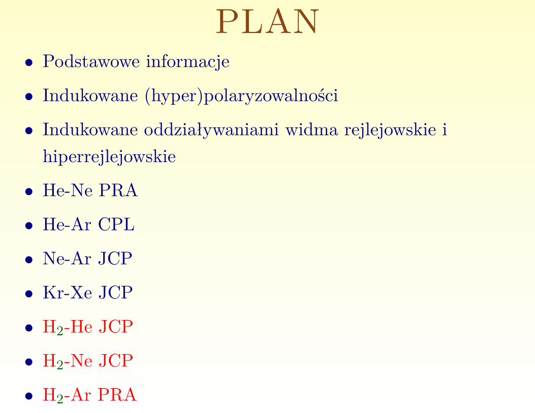
PLAN• Podstawowe informacje
• Indukowane (hyper)polaryzowalności
• Indukowane oddziaływaniami widma rejlejowskie ihiperrejlejowskie
• He-Ne PRA
• He-Ar CPL
• Ne-Ar JCP
• Kr-Xe JCP
• H2-He JCP
• H2-Ne JCP
• H2-Ar PRA
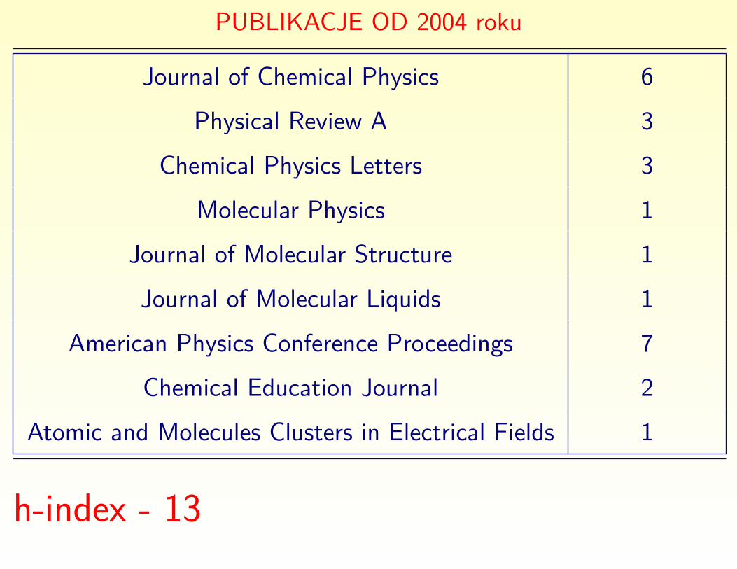
PUBLIKACJE OD 2004 roku
Journal of Chemical Physics 6
Physical Review A 3
Chemical Physics Letters 3
Molecular Physics 1
Journal of Molecular Structure 1
Journal of Molecular Liquids 1
American Physics Conference Proceedings 7
Chemical Education Journal 2
Atomic and Molecules Clusters in Electrical Fields 1
h-index - 13
Atomic and molecular nonlinear optics: Theory, Experiment andComputation, A homage to the pioneering work of StanislawKielich (1925-1993)
Journal Journal of Computational Methods in Science andEngineeringPublisher IOS PressISSN 1472-7978 (Print) 1875-8983Subject Engineering and Technology, Computer-Aided Engineering,Mathematical Analysis and Theory of Computation
Guest Editors G. Maroulis, T. Bancewicz, B. Champagne and A.D.Buckingham

Moi mistrzowie
Stanisław KielichWilliam A. Steele
Yves Le DuffGeorge Maroulis
Granty:
Nieliniowa optyczna spektroskopia supermolekuł 2006-2009 -grantMinistersrwa NiSzW - rozliczony 58 pt na 60.
Spektroskopia optyczna molekuł van-der Waalsa 2010-2013 - grantMNiSzW
Doktoranci: dr Adrian Kamiński - 2011
Z nominacji CK byłem recenzentem rozprawy habilitacyjnej drWiesława Olchawy. Rozprawa odbyła się na UMK w Toruniu
Referaty na zaproszenie
• Spectral Line Shape - Paris 2004 invited talk (z W. Głazem)• Chania 2006 ICCMSE keynote talk (z W. Głazem)• Korfu 2007 ICCMSE keynote talk• Kreta 2008 ICCMSE keynote talk• Rodos 2009 ICCMSE invited talk• Kos 2010 ICCMSE invited talk• First French-Polish Workshop on Organic Electronics andNanophotonics - invited talk - Świeradów Zdrój 2010
Leading Guest Editor in a Special Issue for Journal of Atomic,Molecular, and Optical Physics
Współpraca midzynarodowa:Universite d’Angers; wizyty jako professur invite 2004, 2006, 2007,2009, 2011(dr hab. Jean-Luc Godet) Każda wizyta połączona była zreferatem w Faculte de Sciences, AngersJean-Luc Godet w latach 2004-2010 corocznie odzwiedzał naszWydział
University of Patras, Greece (Professor George Maroulis) 10wspólnych prac
Kairo University (prof. M. El-Kader) - 3 wspólne prace

Fo l low us on Twit t er : @IOSPress_STM
WWW.IOSPRESS.NL
Journal of Computational
Methods in Sciences and
Engineering
Aims and Scope The major goal of the Journal of Computational Methods in Sciences and Engineering (JCMSE) is the publication of new research results on computational methods in sciences and engineering. Common experience had taught us that computational methods originally developed in a given basic science, e.g. physics, can be of paramount importance to other neighbouring sciences, e.g. chemistry, as well as to engineering or technology and, in turn, to society as a whole. This undoubtedly beneficial practice of interdisciplinary interactions will be continuously and systematically encouraged by the JCMSE. Moreover, the JCMSE shall try to simultaneously stimulate similar initiatives, within the realm of computational methods, for knowledge transfer from engineering to applied as well as to basic sciences and beyond. The journal has four sections and welcomes papers on (1) Mathematics and Engineering, (2) Computer Science, (3) Biology and Medicine, and (4) Chemistry and Physics. Editors-in-Chief Prof. Theodore Elias Simos Department of Computer Science and Technology Faculty of Sciences and Technology University of Peloponnese GR-221 00 Tripolis Campus Greece Prof. George Maroulis Department of Chemistry University of Patras GR-26500 Patras Greece Editorial Assistant Mrs. Eleni Ralli-Simou Mathematics and Engineering and Computer Science Prof. Theodore Elias Simos Senior Editors G. Fairweather, N. Hadjisavvas, P. Mezey.
Editors K.J. Bathe, F. Brezzi, M. Calvo, R. De Borst, F.L. Demkovicz, M.J. Donahue, J.M. Ferrandiz, I. Gladwell, B. Gustafsson, G.R. Johnson, A.Q.M. Khaliq, R.W. Lewis, R. Mickens, G. Psihoyios, B.A. Wade, J. Xu. Biology and Medicine and Chemistry and Physics Prof. George Maroulis Senior Editors D. Bonchev, S. Canuto, B. Champagne, M.L. Coote, M. Nakano, M.G. Papadopoulos, C. Pouchan, P. Schwerdtfeger, Z. Slanina, F. Wang, A. Zdetsis. Editors Y. Aoki, P.-O. Åstrand, T. Bancewicz, P. Calaminici, V. Cherepanov, R. Fournier, P. Fuentealba, S.K. Ghosh, F.L. Gu, K. Harigaya, U. Hohm, O. Ivanciuc, L. Jensen, J. Kobus, Z.R. Li, M. Meuwly, M.A. Nunez, P. Piecuch, M. Safronova, M. Swart, H. Tatewaki, A. Thakkar, H. Torii, M. Urban, W.F. Van Gunsteren, M. Weiser, T. Wesolowski, K. Wu, J. Yong Lee. Submission of Papers Authors are requested to send papers on Mathematics and Engineering and Computer Science to Prof. Theodore Elias Simos; [email protected] and papers on Biology and Medicine and Chemistry and Physics to Prof. George Maroulis; [email protected]. Subscription Information Journal of Computational Methods in Sciences and Engineering (ISSN 1472-7978) will be published in 1 volume of 6 issues in 2011 (Volume 10). Institutional subscription (print and online): €657 / US$922 (including postage and handling). Institutional subscription (online only): €600 / US$840. Individual subscription (online only): €175 / US$210. Abstracted / Indexed in Chemical Abstracts, Inspec, Mathematical Reviews, MathSciNet, Zentralblatt MATH.
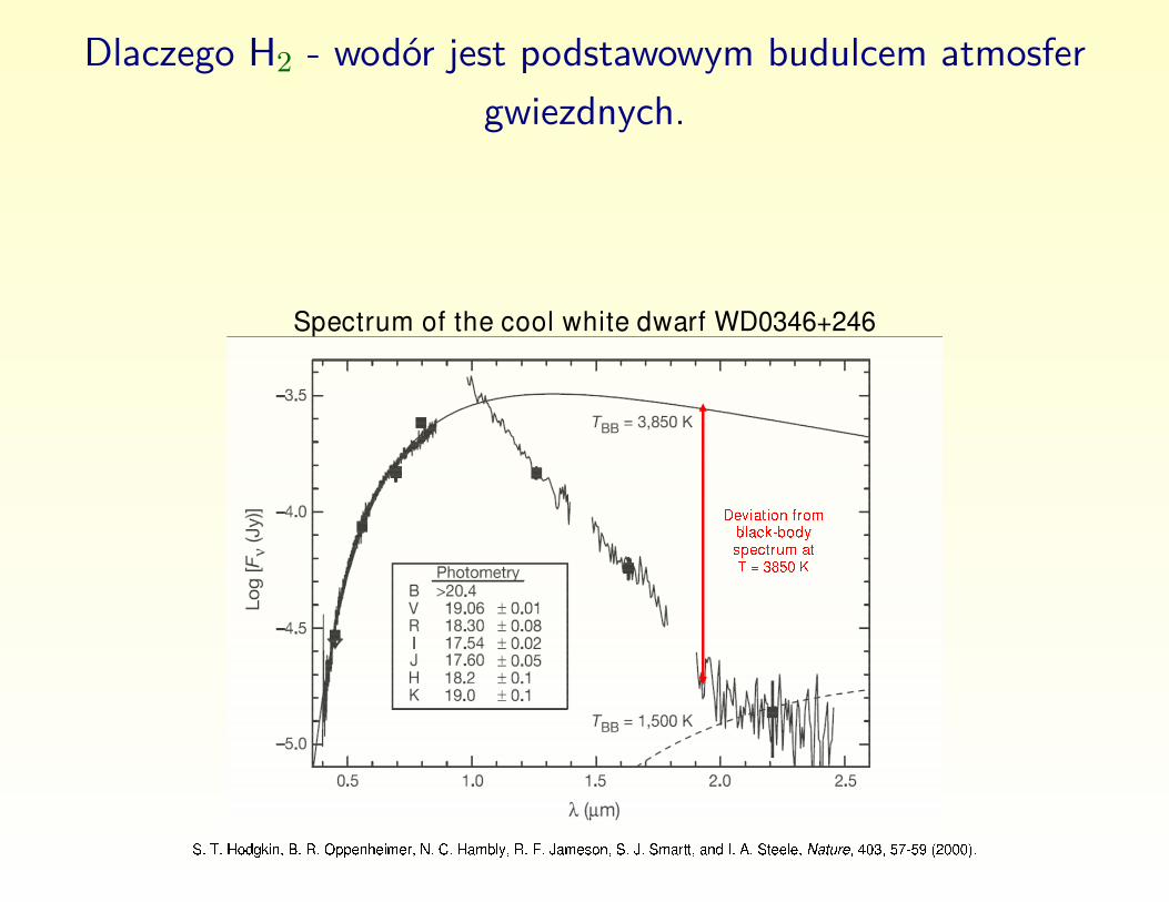
Dlaczego H2 - wodór jest podstawowym budulcem atmosfergwiezdnych.
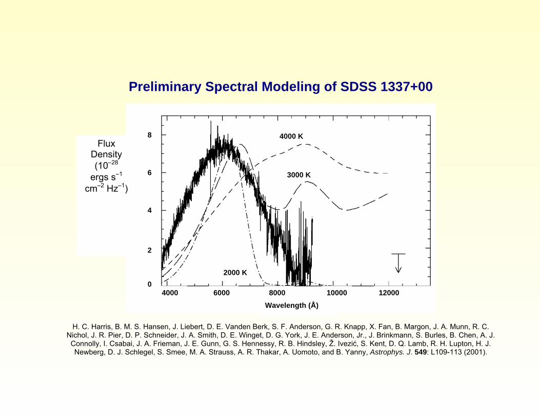
Preliminary Spectral Modeling of SDSS 1337+00
8 6 4 2 0
Flux Density (10−28
ergs s−1 cm−2 Hz−1)
4000
4000 K
3000 K
2000 K
6000
10000 Wavelength (Å) 8000 12000
H. C. Harris, B. M. S. Hansen, J. Liebert, D. E. Vanden Berk, S. F. Anderson, G. R. Knapp, X. Fan, B. Margon, J. A. Munn, R. C. Nichol, J. R. Pier, D. P. Schneider, J. A. Smith, D. E. Winget, D. G. York, J. E. Anderson, Jr., J. Brinkmann, S. Burles, B. Chen, A. J.
Connolly, I. Csabai, J. A. Frieman, J. E. Gunn, G. S. Hennessy, R. B. Hindsley, Ž. Ivezić, S. Kent, D. Q. Lamb, R. H. Lupton, H. J. Newberg, D. J. Schlegel, S. Smee, M. A. Strauss, A. R. Thakar, A. Uomoto, and B. Yanny, Astrophys. J. 549: L109-113 (2001).
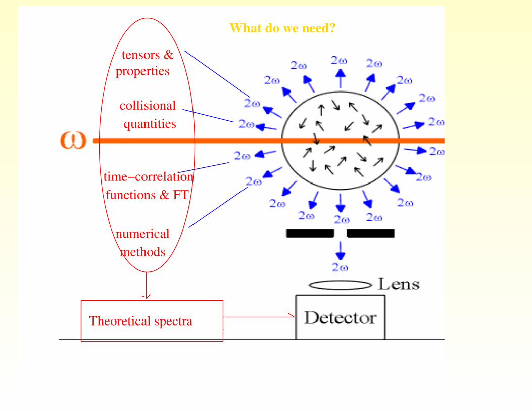
collisional
quantities
tensors &
properties
time−correlation
functions & FT
numerical
methods
Theoretical spectra
What do we need?
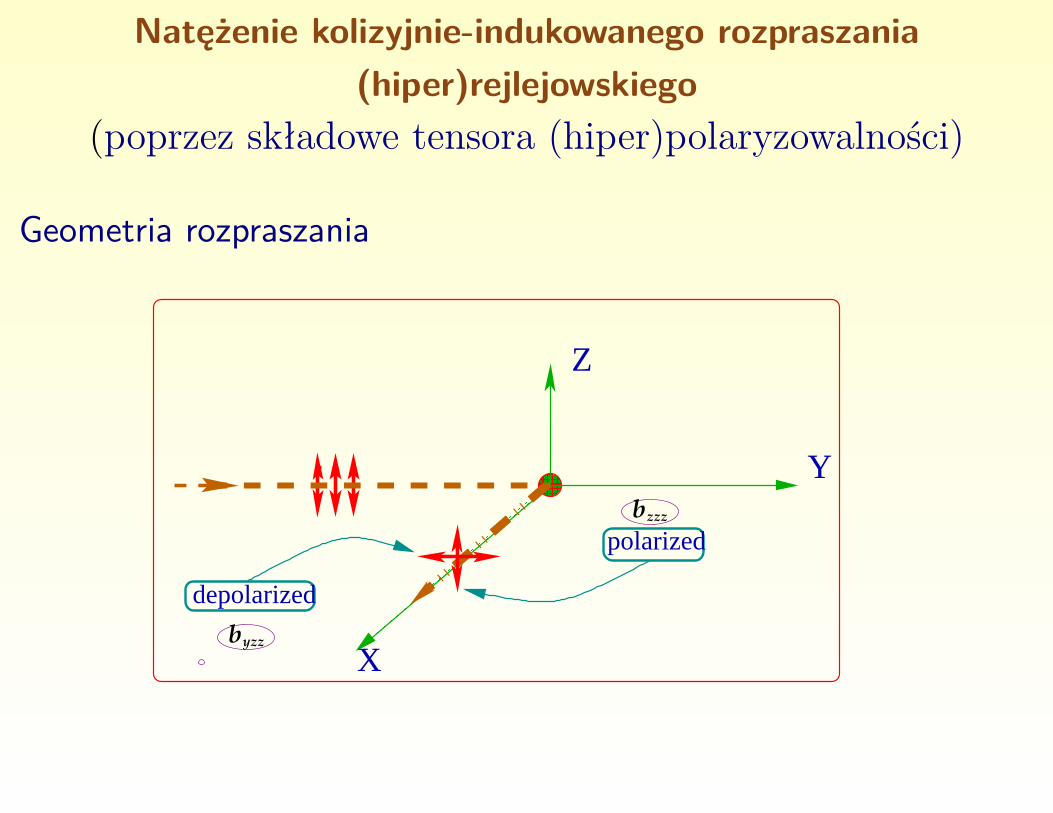
Natężenie kolizyjnie-indukowanego rozpraszania(hiper)rejlejowskiego
(poprzez składowe tensora (hiper)polaryzowalności)
Geometria rozpraszania
Y
X
polarized
depolarized
Z
b
bzzz
yzz
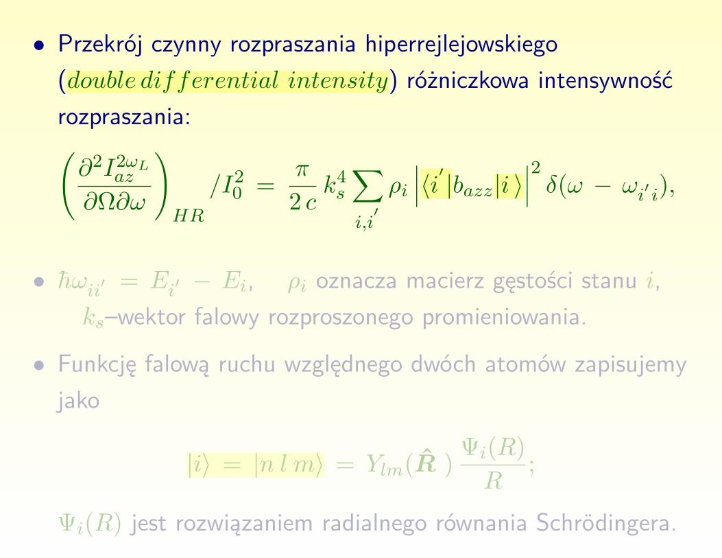
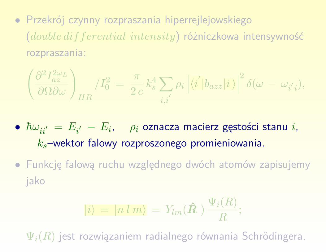
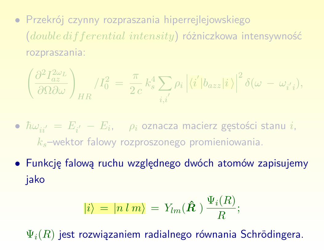
• Przekrój czynny rozpraszania hiperrejlejowskiego(double differential intensity) różniczkowa intensywnośćrozpraszania:(∂2I2ωLaz∂Ω∂ω
)HR
/I20 = π
2 ck4s
∑i,i′
ρi∣∣∣〈i′ |bazz|i 〉∣∣∣2 δ(ω − ωi′ i),
• hωii′ = Ei′ − Ei, ρi oznacza macierz gęstości stanu i,ks–wektor falowy rozproszonego promieniowania.
• Funkcję falową ruchu względnego dwóch atomów zapisujemyjako
|i〉 = |n l m〉 = Ylm(R ) Ψi(R)R
;
Ψi(R) jest rozwiązaniem radialnego równania Schrödingera.
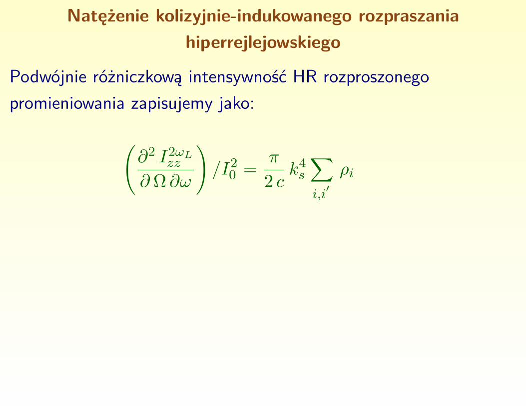
Natężenie kolizyjnie-indukowanego rozpraszaniahiperrejlejowskiego
Podwójnie różniczkową intensywność HR rozproszonegopromieniowania zapisujemy jako:
(∂2 I2ωLzz∂ Ω ∂ω
)/I20 = π
2 ck4s
∑i,i′
ρi
(1)
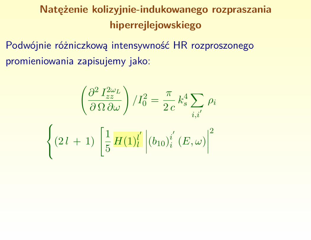
Natężenie kolizyjnie-indukowanego rozpraszaniahiperrejlejowskiego
Podwójnie różniczkową intensywność HR rozproszonegopromieniowania zapisujemy jako:
(∂2 I2ωLzz∂ Ω ∂ω
)/I20 = π
2 ck4s
∑i,i′
ρi
(2 l + 1)[
15H(1)l
′
l
∣∣∣∣(b10)i′
i (E,ω)∣∣∣∣2
(1)
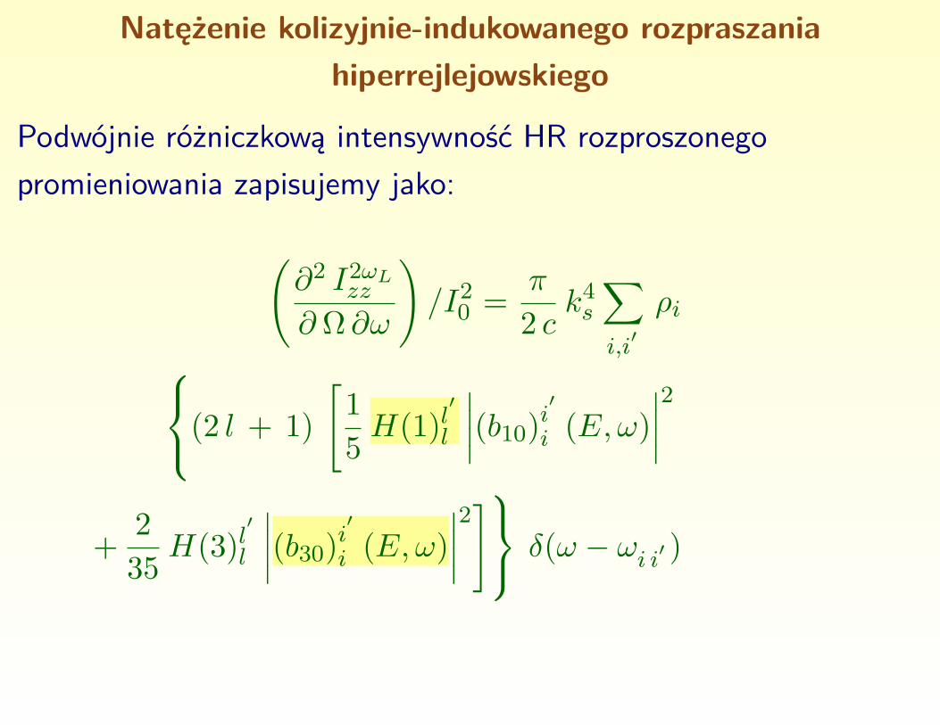
Natężenie kolizyjnie-indukowanego rozpraszaniahiperrejlejowskiego
Podwójnie różniczkową intensywność HR rozproszonegopromieniowania zapisujemy jako:
(∂2 I2ωLzz∂ Ω ∂ω
)/I20 = π
2 ck4s
∑i,i′
ρi
(2 l + 1)[
15H(1)l
′
l
∣∣∣∣(b10)i′
i (E,ω)∣∣∣∣2
+ 235H(3)l
′
l
∣∣∣∣(b30)i′
i (E,ω)∣∣∣∣2] δ(ω − ωi i′ )
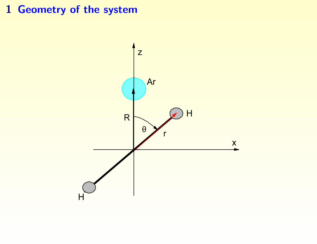
1 Geometry of the system
A r
H
H
rR
z
θx
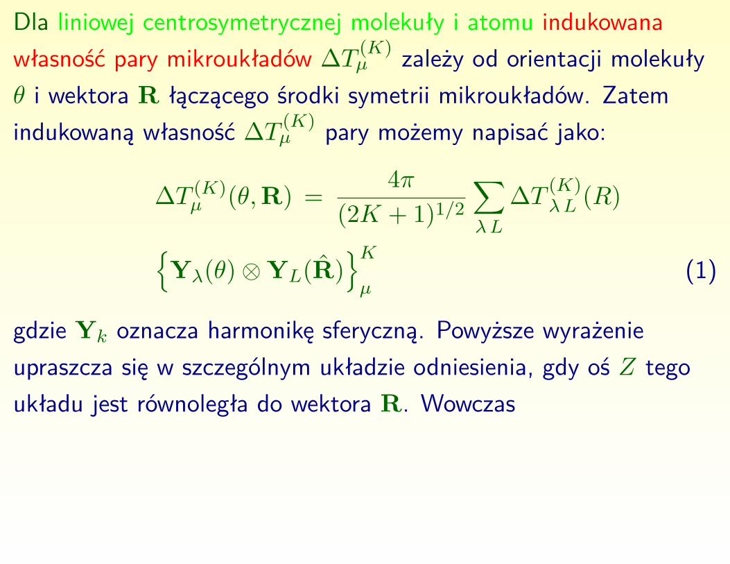
Dla liniowej centrosymetrycznej molekuły i atomu indukowanawłasność pary mikroukładów ∆T (K)
µ zależy od orientacji molekułyθ i wektora R łączącego środki symetrii mikroukładów. Zatemindukowaną własność ∆T (K)
µ pary możemy napisać jako:
∆T (K)µ (θ,R) = 4π
(2K + 1)1/2
∑λL
∆T (K)λL (R)
Yλ(θ)⊗YL(R)
Kµ
(1)
gdzie Yk oznacza harmonikę sferyczną. Powyższe wyrażenieupraszcza się w szczególnym układzie odniesienia, gdy oś Z tegoukładu jest równoległa do wektora R. Wowczas
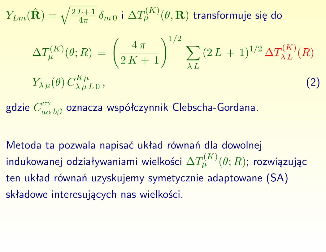
YLm(R) =√
2L+ 14π δm 0 i ∆T (K)
µ (θ,R) transformuje się do
∆T (K)µ (θ;R) =
(4π
2K + 1
)1/2 ∑λL
(2L + 1)1/2 ∆T (K)λL (R)
Yλµ(θ)CKµλµL 0 , (2)
gdzie Ccγaα bβ oznacza współczynnik Clebscha-Gordana.
Metoda ta pozwala napisać układ równań dla dowolnejindukowanej odziaływaniami wielkości ∆T (K)
µ (θ;R); rozwiązującten układ równań uzyskujemy symetycznie adaptowane (SA)składowe interesujących nas wielkości.
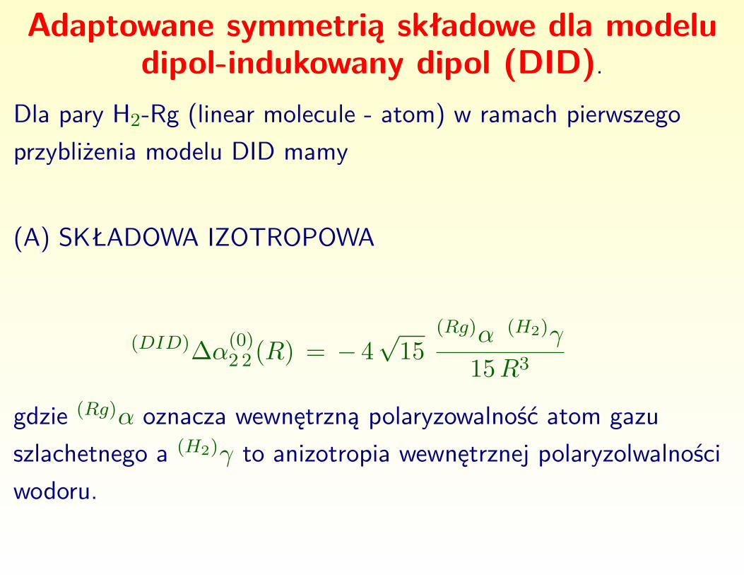
Adaptowane symmetrią składowe dla modeludipol-indukowany dipol (DID).
Dla pary H2-Rg (linear molecule - atom) w ramach pierwszegoprzybliżenia modelu DID mamy
(A) SKŁADOWA IZOTROPOWA
(DID)∆α(0)2 2 (R) = − 4
√15
(Rg)α (H2)γ
15R3
gdzie (Rg)α oznacza wewnętrzną polaryzowalność atom gazuszlachetnego a (H2)γ to anizotropia wewnętrznej polaryzolwalnościwodoru.
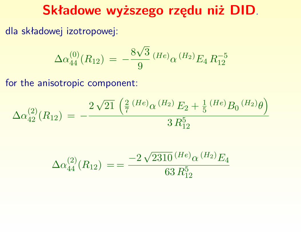
Składowe wyższego rzędu niż DID.
dla składowej izotropowej:
∆α(0)44 (R12) = −8
√3
9(He)α (H2)E4R
−512
for the anisotropic component:
∆α(2)42 (R12) = −
2√
21(
27
(He)α (H2)E2 + 15
(He)B0(H2)θ
)3R5
12
∆α(2)44 (R12) = = −2
√2310 (He)α (H2)E4
63R512
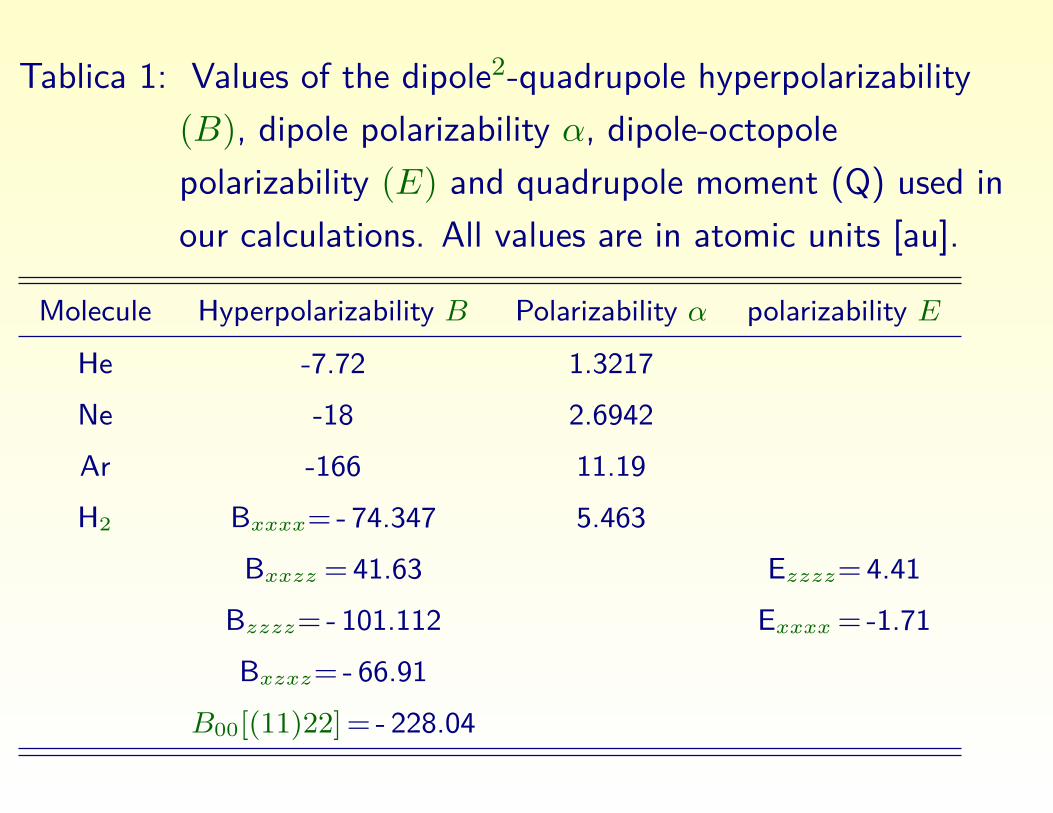
Tablica 1: Values of the dipole2-quadrupole hyperpolarizability(B), dipole polarizability α, dipole-octopolepolarizability (E) and quadrupole moment (Q) used inour calculations. All values are in atomic units [au].
Molecule Hyperpolarizability B Polarizability α polarizability E
He -7.72 1.3217Ne -18 2.6942Ar -166 11.19H2 Bxxxx= - 74.347 5.463
Bxxzz = 41.63 Ezzzz= 4.41Bzzzz= - 101.112 Exxxx= -1.71Bxzxz= - 66.91
B00[(11)22] = - 228.04
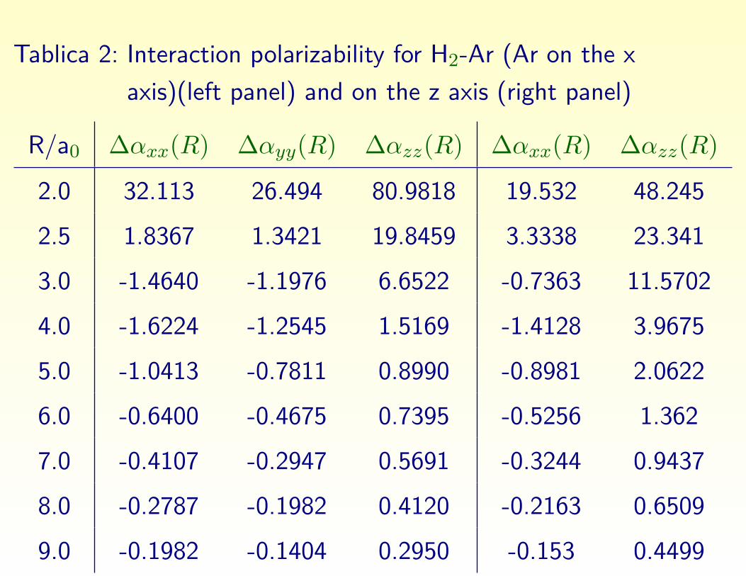
Tablica 2: Interaction polarizability for H2-Ar (Ar on the xaxis)(left panel) and on the z axis (right panel)
R/a0 ∆αxx(R) ∆αyy(R) ∆αzz(R) ∆αxx(R) ∆αzz(R)
2.0 32.113 26.494 80.9818 19.532 48.245
2.5 1.8367 1.3421 19.8459 3.3338 23.341
3.0 -1.4640 -1.1976 6.6522 -0.7363 11.5702
4.0 -1.6224 -1.2545 1.5169 -1.4128 3.9675
5.0 -1.0413 -0.7811 0.8990 -0.8981 2.0622
6.0 -0.6400 -0.4675 0.7395 -0.5256 1.362
7.0 -0.4107 -0.2947 0.5691 -0.3244 0.9437
8.0 -0.2787 -0.1982 0.4120 -0.2163 0.6509
9.0 -0.1982 -0.1404 0.2950 -0.153 0.4499
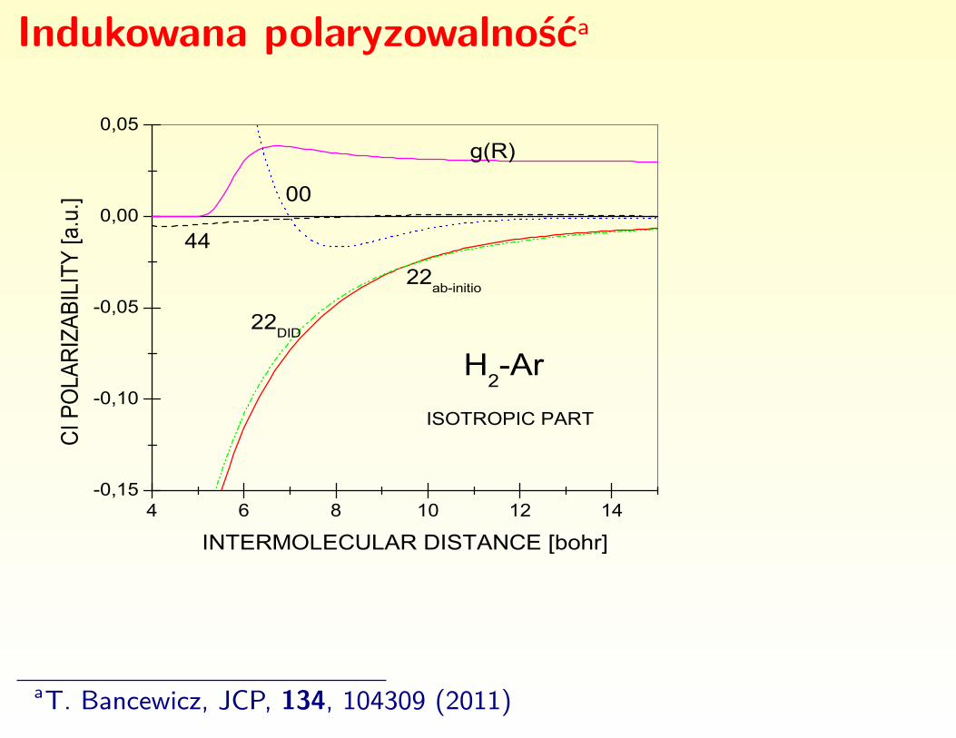
Indukowana polaryzowalnośća
4 6 8 1 0 1 2 1 4- 0 , 1 5
- 0 , 1 0
- 0 , 0 5
0 , 0 0
0 , 0 5
H 2 - A r
CI PO
LARIZ
ABILIT
Y [a.u
.]
I N T E R M O L E C U L A R D I S T A N C E [ b o h r ]
0 04 4
I S O T R O P I C P A R T
2 2 a b - i n i t i o
2 2 D I D
g ( R )
aT. Bancewicz, JCP, 134, 104309 (2011)
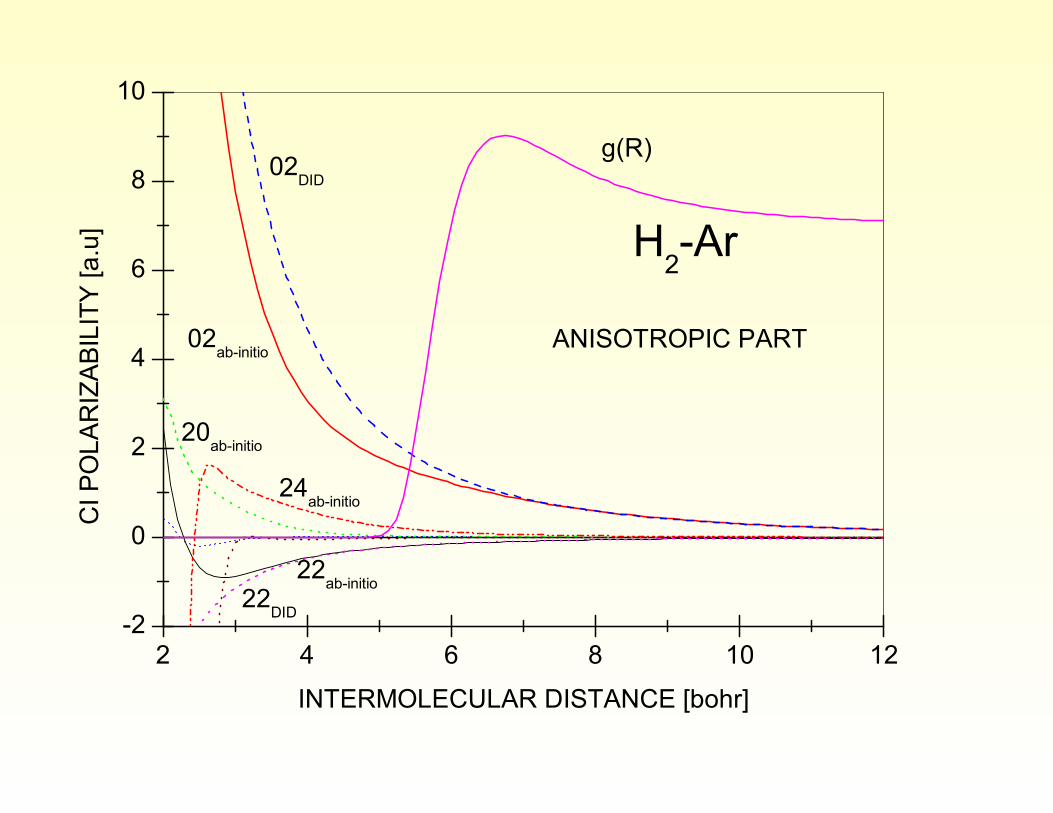
2 4 6 8 1 0 1 2- 2
0
2
4
6
8
1 0
H 2 - A r
CI PO
LARIZ
ABILI
TY [a
.u]
I N T E R M O L E C U L A R D I S T A N C E [ b o h r ]
0 2 D I D
0 2 a b - i n i t i o
2 2 a b - i n i t i o2 2 D I D
2 0 a b - i n i t i o
2 4 a b - i n i t i o
A N I S O T R O P I C P A R T
g ( R )
Rysunek 1: σ=5.71bohr
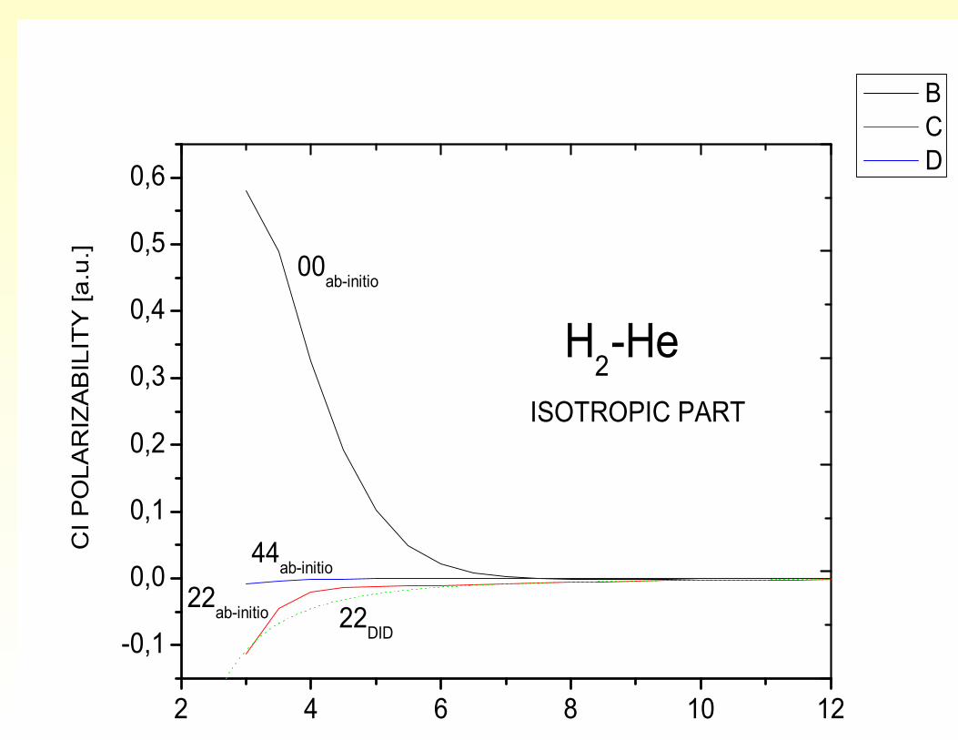
2 4 6 8 1 0 1 2- 0 , 10 , 00 , 10 , 20 , 30 , 40 , 50 , 6
CI P
OLAR
IZABI
LITY
[a.u.]
I N T E R M O L E C U L A R D I S T A N C E [ b o h r ]
B C D
0 0 a b - i n i t i o
2 2 a b - i n i t i o
4 4 a b - i n i t i o
2 2 D I D
H 2 - H eI S O T R O P I C P A R T
Rysunek 2: σ=5.71bohr
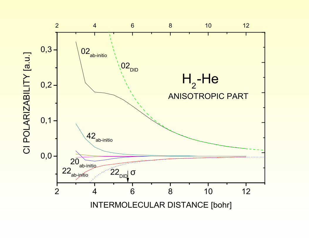
2 4 6 8 1 0 1 2
0 , 0
0 , 1
0 , 2
0 , 3
2 4 6 8 1 0 1 2CI
POLA
RIZAB
ILITY
[a.u.
]
I N T E R M O L E C U L A R D I S T A N C E [ b o h r ]
0 2 a b - i n i t i o
2 0 a b - i n i t i o2 2 a b - i n i t i o
4 2 a b - i n i t i o
0 2 D I D
2 2 D I D
A N I S O T R O P I C P A R T
σ
H 2 - H e
Rysunek 3:
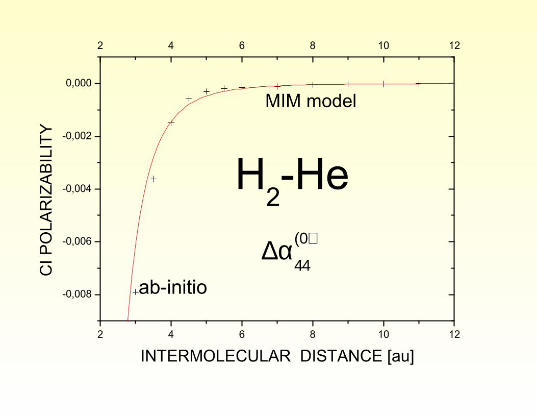
2 4 6 8 1 0 1 2
- 0 , 0 0 8
- 0 , 0 0 6
- 0 , 0 0 4
- 0 , 0 0 2
0 , 0 0 0
2 4 6 8 1 0 1 2CI
POLA
RIZAB
ILITY
I N T E R M O L E C U L A R D I S T A N C E [ a u ]
H 2 - H ea b - i n i t i o
M I M m o d e l
∆α(0)
44
Rysunek 4:
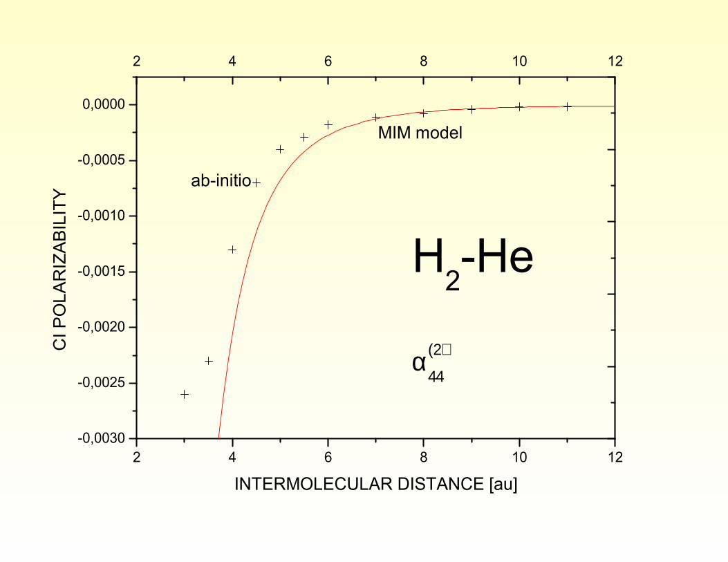
2 4 6 8 1 0 1 2- 0 , 0 0 3 0
- 0 , 0 0 2 5
- 0 , 0 0 2 0
- 0 , 0 0 1 5
- 0 , 0 0 1 0
- 0 , 0 0 0 5
0 , 0 0 0 0
2 4 6 8 1 0 1 2CI
POLA
RIZA
BILITY
I N T E R M O L E C U L A R D I S T A N C E [ a u ]
H 2 - H ea b - i n i t i o
M I M m o d e l
α(2)
44
Rysunek 5:

2 4 6 8 1 0 1 2 1 4
- 0 , 0 0 8
- 0 , 0 0 6
- 0 , 0 0 4
- 0 , 0 0 2
0 , 0 0 0
2 4 6 8 1 0 1 2 1 4CI
POLA
RIZAB
ILITY
I N T E R M O L E C U L A R D I S T A N C E [ a u ]
H 2 - N e∆α(0)
44
M I M m o d e la b - i n i t i o
Rysunek 6:
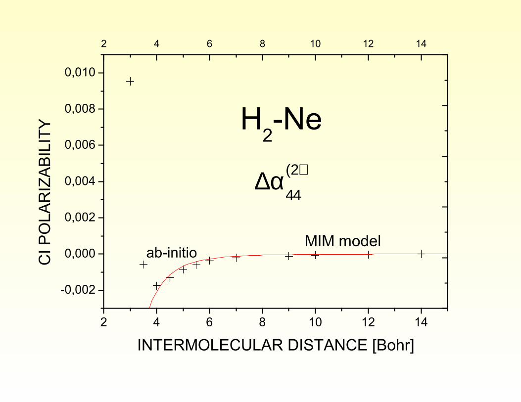
2 4 6 8 1 0 1 2 1 4
- 0 , 0 0 2
0 , 0 0 0
0 , 0 0 2
0 , 0 0 4
0 , 0 0 6
0 , 0 0 8
0 , 0 1 02 4 6 8 1 0 1 2 1 4
CI PO
LARIZ
ABILI
TY
I N T E R M O L E C U L A R D I S T A N C E [ B o h r ]
H 2 - N e
a b - i n i t i o M I M m o d e l
∆α(2)
44
Rysunek 7:
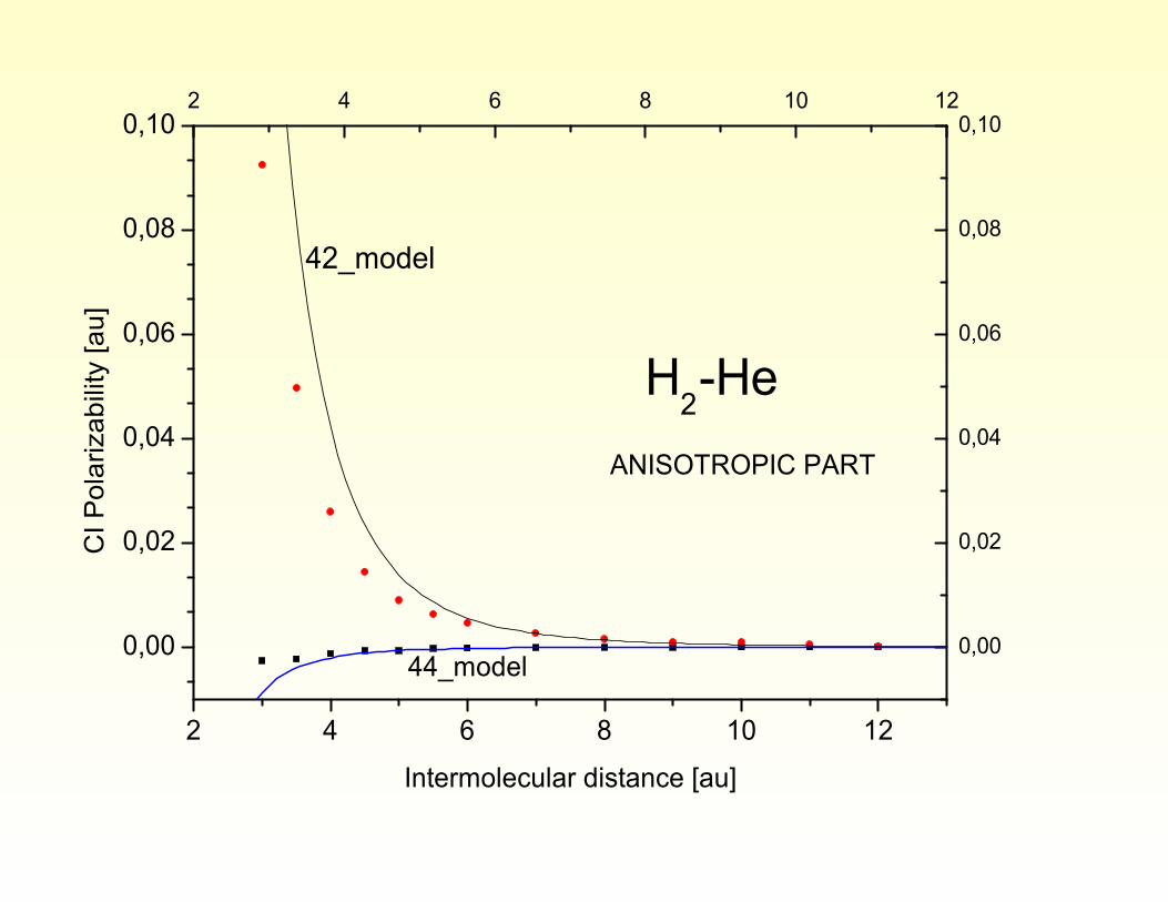
2 4 6 8 1 0 1 2
0 , 0 0
0 , 0 2
0 , 0 4
0 , 0 6
0 , 0 8
0 , 1 0 2 4 6 8 1 0 1 2
0 , 0 0
0 , 0 2
0 , 0 4
0 , 0 6
0 , 0 8
0 , 1 0CI
Polar
izabil
ity [a
u]
I n t e r m o l e c u l a r d i s t a n c e [ a u ]
4 2 _ m o d e l
4 4 _ m o d e l
H 2 - H eA N I S O T R O P I C P A R T
Rysunek 8:
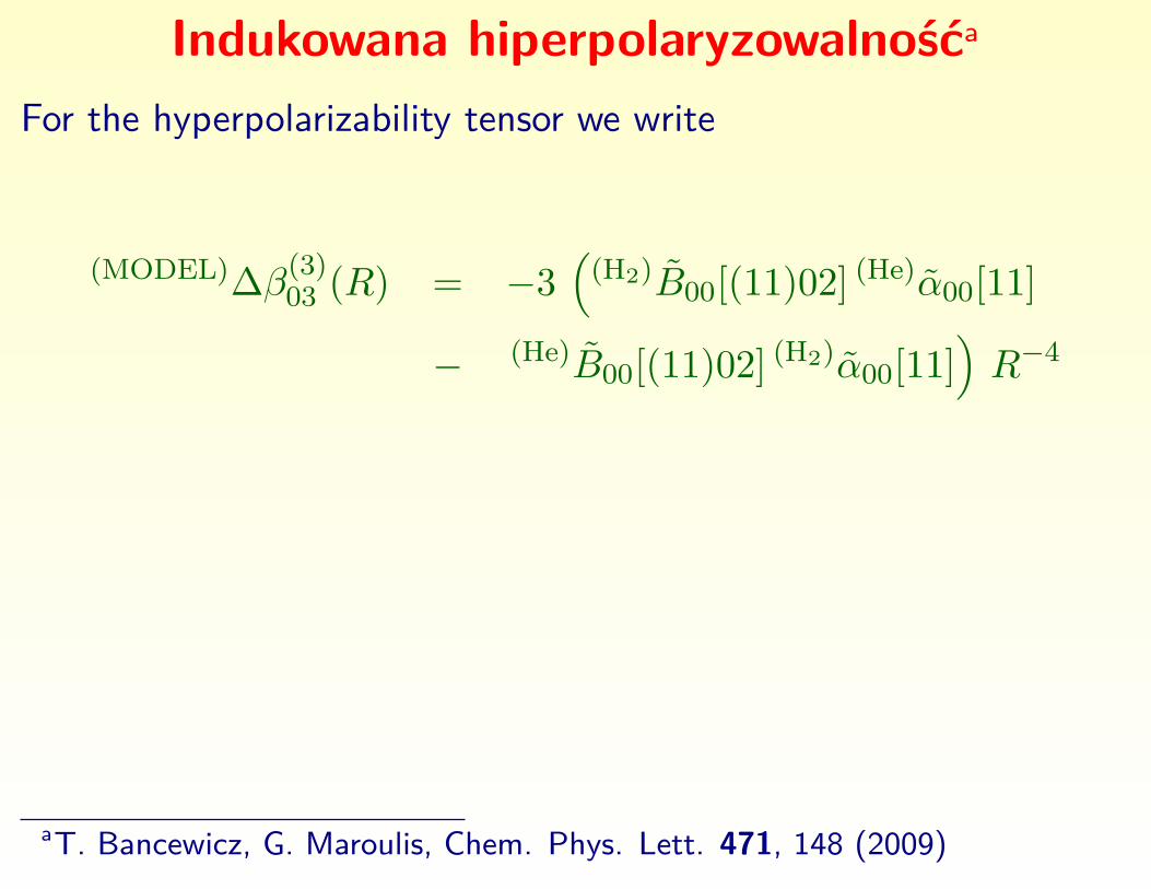
Indukowana hiperpolaryzowalnośća
For the hyperpolarizability tensor we write
(MODEL)∆β(3)03 (R) = −3
((H2)B00[(11)02] (He)α00[11]
− (He)B00[(11)02] (H2)α00[11])R−4
aT. Bancewicz, G. Maroulis, Chem. Phys. Lett. 471, 148 (2009)
2 4 6 8 1 0 1 2 1 4 1 6
- 1
0
1
2
3
4
5
62 4 6 8 1 0 1 2 1 4 1 6
0
2
4
6CI
HYPE
RPOL
ARIZA
BILITY
[au]
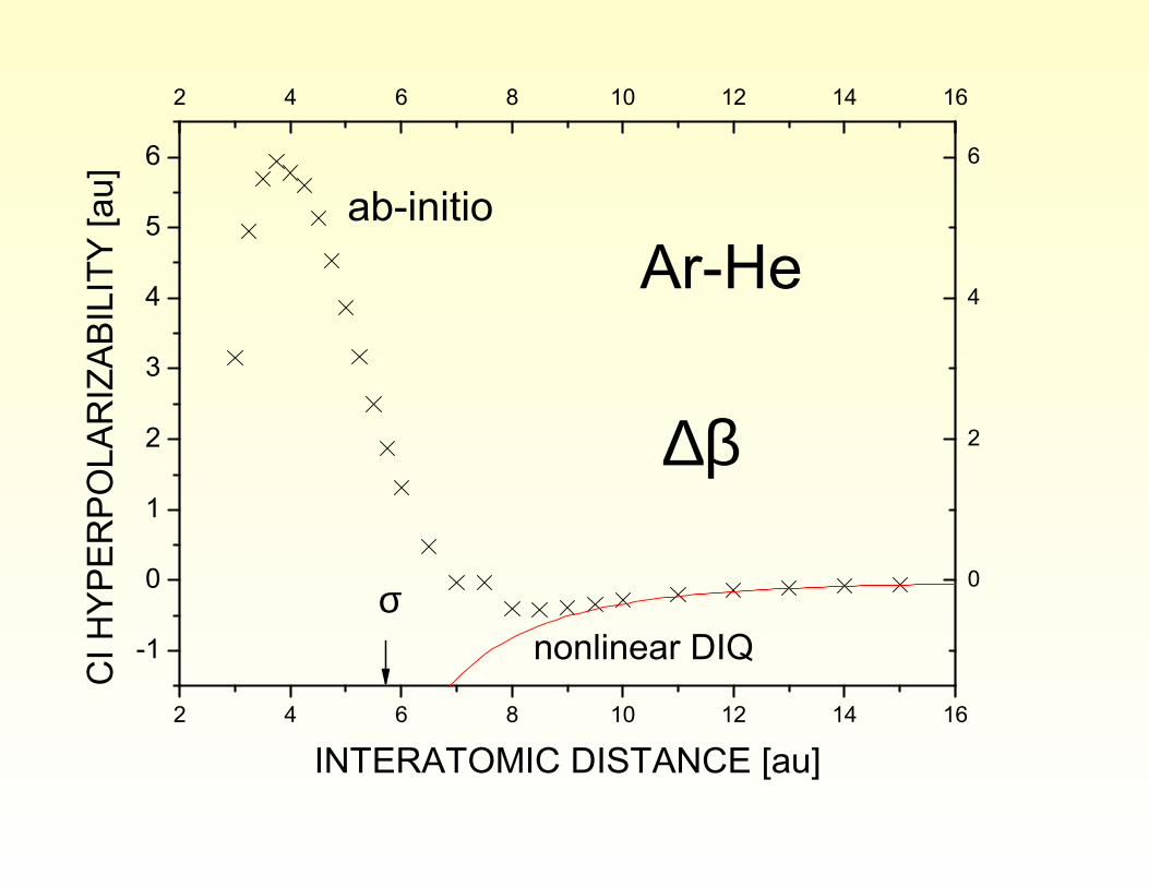
I N T E R A T O M I C D I S T A N C E [ a u ]
a b - i n i t i o
n o n l i n e a r D I Q
∆β
A r - H e
σ
Rysunek 9:
2 4 6 8 1 0- 0 , 3 0
- 0 , 2 5
- 0 , 2 0
- 0 , 1 5
- 0 , 1 0
- 0 , 0 5
0 , 0 0
0 , 0 5
0 , 1 0 2 4 6 8 1 0CI
HYPE
RPOL
ARIZA
BILITY
[au]
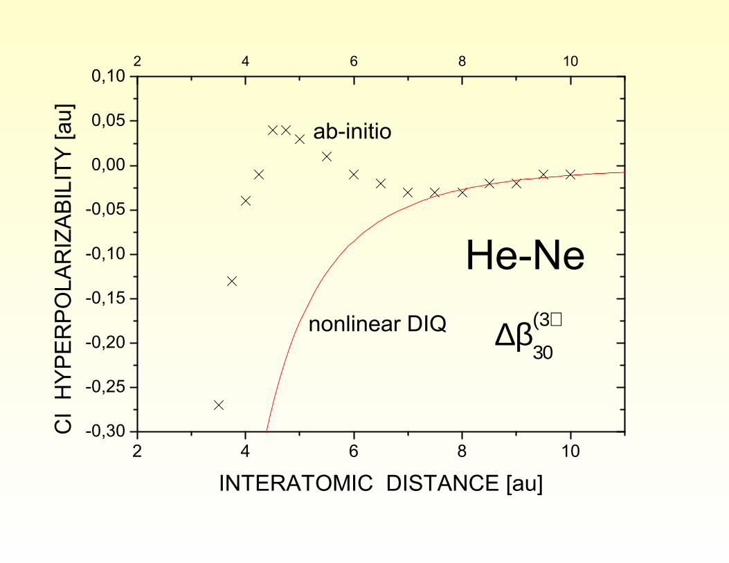
I N T E R A T O M I C D I S T A N C E [ a u ]
H e - N e∆β(3)
30
a b - i n i t i o
n o n l i n e a r D I Q
Rysunek 10:
4 6 8 1 0 1 2 1 4 1 6 1 8 2 0 2 2 2 4 2 6- 1 0
- 8
- 6
- 4
- 2
0
2
44 6 8 1 0 1 2 1 4 1 6 1 8 2 0 2 2 2 4 2 6
CI HY
PERP
OLAR
IZABIL
ITY [a
u]
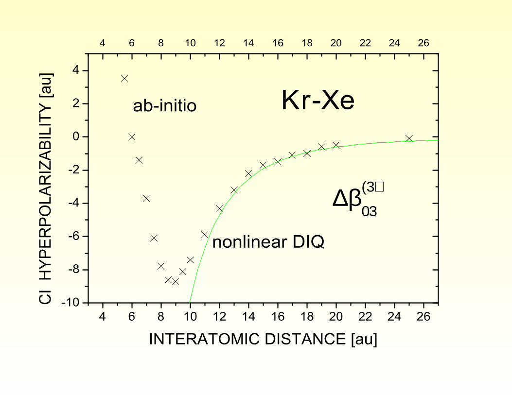
I N T E R A T O M I C D I S T A N C E [ a u ]
K r - X ea b - i n i t i o
n o n l i n e a r D I Q∆β(3)
03
Rysunek 11:
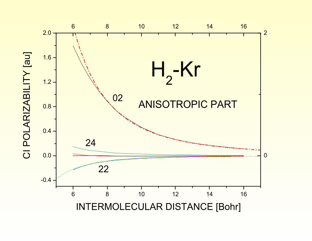
6 8 1 0 1 2 1 4 1 6- 0 . 4
0 . 0
0 . 4
0 . 8
1 . 2
1 . 6
2 . 06 8 1 0 1 2 1 4 1 6
0
2CI
POLA
RIZAB
ILITY
[au]
I N T E R M O L E C U L A R D I S T A N C E [ B o h r ]
0 2
2 2
2 4
H 2 - K rA N I S O T R O P I C P A R T
Rysunek 12:

DZIĘKUJĘ ZA POŚWIĘCONĄ UWAGĘ


![Wstep˛ do Optyki i Fizyki Materii Skondensowanej[patlah.ru] Podstawy spektroskopii Spektroskopia w zastosowaniach Spektroskopia absorpcyjna Badania struktury energetycznej" A portion](https://img.pdfslide.tips/doc/110x75/60e21ca3a9d83b369c5540a5/wstep-do-optyki-i-fizyki-materii-skondensowanej-patlahru-podstawy-spektroskopii.jpg)